self-learning backlash inverse control of cooling or
TRANSCRIPT
Purdue UniversityPurdue e-PubsInternational Refrigeration and Air ConditioningConference School of Mechanical Engineering
2016
Self-learning Backlash Inverse Control of Coolingor Heating Coil Valves Having Backlash HysteresisJie CaiRay W. Herrick Laboratories, Purdue University, United States of America, [email protected]
James E. BraunRay W. Herrick Laboratories, Purdue University, United States of America, [email protected]
Follow this and additional works at: http://docs.lib.purdue.edu/iracc
This document has been made available through Purdue e-Pubs, a service of the Purdue University Libraries. Please contact [email protected] foradditional information.Complete proceedings may be acquired in print and on CD-ROM directly from the Ray W. Herrick Laboratories at https://engineering.purdue.edu/Herrick/Events/orderlit.html
Cai, Jie and Braun, James E., "Self-learning Backlash Inverse Control of Cooling or Heating Coil Valves Having Backlash Hysteresis"(2016). International Refrigeration and Air Conditioning Conference. Paper 1801.http://docs.lib.purdue.edu/iracc/1801
2577, Page 1
16th
International Refrigerat ion and Air Conditioning Conference at Purdue, Ju ly 11-14, 2016
Self-Learning Backlash Inverse Control of Cooling or Heating Coil Valves Having
Backlash Hysteresis
Jie CAI
1*, James E. BRAUN
1
1Ray W. Herrick Laboratories, Purdue University, West Lafayette, IN, USA
* Corresponding Author
ABSTRACT
Valves are widely used in HVAC systems to regulate liquid flow rate, such as hot - and chilled-water valves utilized
in cooling and heating coils. These valves are typically controlled with motorized actuators where significant
backlash hysteresis might exist and the backlash magnitude mostly depends on the clearance of the manufactured
gearbox. Due to the hysteresis effect, unsatisfactory tracking performance results when using a conventional PI
controller. To understand the control effect from the backlash hysteresis, this paper develops an emulator model for
a cooling coil and valve set derived from field measurements. Based on observations of the simulation results, a self-
learning backlash inverse control approach is proposed to mit igate the backlash effect with moderate modifications
to a conventional PI control. In the proposed approach, a self-learn ing procedure is carried out at the beginning of
the control implementation period to estimate the backlash magnitude for a specific valve. Then a backlash inverse
block is added to an existing PI controller to compensate for the hysteresis effect residing in the valve. The validity
of the proposed method was verified with both simulation and experimental tests and significant improvement was
observed in the control performance.
1. INTRODUCTION
Valves are commonly used in industrial and commercial applications to regulate liquid flow rate for various
purposes. In build ing HVAC systems, valves are employed for regulation of hot- and chilled-water in cooling and
heating coils to control the heat exchange rate. For valves with automatic control capability, motorized actuators are
typically utilized for driv ing a valve to open or close based on a control command provided by a feedback controller.
Backlash type hysteresis often exists in an actuator gearbox where the stem position differs at a given input
command when the actuation changes its direction, causing difficult ies in obtaining a stable control. The hysteresis
magnitude depends on the manufacturing clearance that can vary significantly even for the same batch of products.
This study was motivated by the unsatisfactory comfort control that had been observed in the HVAC system serving
multip le offices that are Living Laboratories fo r the Center fo r High Performance Buildings at Purdue University.
The unsatisfactory performance was main ly caused by valve hysteresis residing in the chilled- and hot-water valves.
Conventional PID controllers were not able to provide stable control due to the valve hysteresis and the control
variables were observed to oscillate significantly. As a consequence, space temperatures fluctuated and comfort
requirements could not be satisfied. A companion paper (Cai, Kurtu lus and Braun, 2016) presented a comprehensive
set of experimental test results comparing different valve characteristics in variable -air-volume (VAV) box reheat
and air handling unit (AHU) cooling coil valves and investigated their impacts on control performance. The results
showed severe control temperature fluctuations for valves having significant backlash-type hysteresis. In addition,
the control fluctuations led to unnecessarily high cooling/heating power so demand costs would be raised for
buildings subject to demand charges. Backlash-type hysteresis commonly exists in HVAC valves due to the
relatively low manufacturing tolerances employed and emphasis on low cost solutions . All position controlled
valves that were surveyed in Cai et al. (2016) suffered from significant backlash hysteresis (more than 5%). Thus, a
specifically devised control approach for handling such backlash-type hysteresis could bring tremendous benefits for
buildings in energy cost reduction and improved comfort.

2577, Page 2
16th
International Refrigerat ion and Air Conditioning Conference at Purdue, Ju ly 11-14, 2016
Backlash inverse control has been studied extensively in the control community as an effective approach to mitigate
backlash-type hysteresis in a control system. The backlash inverse controller is typically implemented in series with
a typical feedback controller, e .g., PI controller, to compensate for backlash-type non-linearity. For systems with
unknown backlash sizes, adaptive inverse control is often utilized to estimate and adapt the backlash size (Tao and
Kokotovic, 1993, Tao and Kokotovic, 1996 and Ahmad and Khorrami, 1999). However, most of the adaptive laws
in the previous work are only valid for linear systems and very few studies considered case studies with nonlinear
plants.
Hagglund (2007) proposed an on-line estimat ion algorithm for backlash magnitude based on closed-loop operation
data. The on-line estimat ion step achieved a similar goal to the self-learn ing process proposed in the current study.
But the estimation mechanism is different: Hagglund (2007) utilized the delay time and magnitude in the system
reaction to infer the backlash size that requires informat ion of the PI control settings and estimation of the plant
static process gain. In addition, the backlash estimation quality highly depends on external disturbances. The self-
learning process within the present paper, however, is based on simple observations in the control behavior and no
informat ion is needed in terms of plant characteristics or PI control settings. In addition, it is more robust in handling
external d isturbances.
Some previous research work studied dynamic modeling of hydronic valves with hysteresis to enable controller
design and performance assessment. For example, Kumar and Mittal (2010) developed a dynamic model o f the
liquid flow process within a regulation valve. A hysteresis model was incorporated to capture the hysteresis effect
and the overall model p rovided a simulation test bed to investigate different valve control approaches. Tudoroiu and
Zaheeruddin (2005) considered a similar case study as the present paper where the valve backlash hysteresis effect
on control performance of a discharge air temperature system was studied. The paper relied on a dynamic simulation
model to investigate the backlash effect and fluctuations were observed in the discharge air te mperature when valve
backlash magnitude was increased gradually. However, the study mainly focused on the fault detection problem
without addressing the control problem.
This paper focuses on the development of data-driven cooling coil and valve models that are useful in understanding
control stability issues caused by valve hysteresis and in developing controllers to mit igate the backlash hysteresis
effect leading to improved control performance. Based on the observed control chattering patterns , a self-learning
approach is proposed to estimate the backlash magnitude and a corresponding backlash inverse controller is
implemented to improve the control performance. The effect iveness of this approach has been demonstrated via both
simulation and experimental tests although only simulation results will be presented in this paper due to space
limitat ions. Note that the proposed self-learning backlash inverse control approach is generally applicable for
hydronic valves although only a HVAC applicat ion is demonstrated here.
2. VALVE AND COOLING COIL DATA-DRIVEN MODELS
A valve model with hysteresis effects and a dynamic cooling coil model were developed based on field
measurements from the Living Labs at Purdue University. Details of the experimental setup were presented in the
companion paper by Cai, Kurtu lus and Braun (2016). These models are combined in a simulation tool for
understanding, developing and validating the backlash inverse control approach.
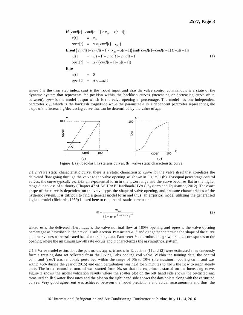
2.1 Valve Models 2.1.1 Valve hysteresis model: the actuation of valve opening in response to control command follows a dynamic
behavior because of the inherent hysteresis where the valve opening does not only depend on the current control
command but also requires informat ion of the prev ious control action to determine the current actuation status in the
backlash region (on the increasing or decreasing curve or in between, as shown in Figure 1 (a)). A discrete-time
backlash dynamic model can be formulated as
2577, Page 3
16th
International Refrigerat ion and Air Conditioning Conference at Purdue, Ju ly 11-14, 2016
[ ] [ 1] [ 1]
[ ]
[ ] [ ]
[ ] [ 1] [ 1] [ ] [ 1] [ 1]
[ ] [ 1] [ ] [ 1]
[ ] [ 1] [ 1]
[ ] 0
[ ] [ ]
BL
BL
BL
BL
cmd t cmd t x x t
x t x
open t cmd t x
cmd t cmd t x x t cmd t cmd t x t
x t x t cmd t cmd t
open t cmd t x t
x t
open t cmd t
If
Elseif and
Else
(1)
where t is the time step index, cmd is the model input and also the valve control command, x is a state of the
dynamic system that represents the position within the backlash curves (increasing or decreasing curve or in
between), open is the model output which is the valve opening in percentage. The model has one independent
parameter xBL, which is the backlash magnitude while the parameter α is a dependent parameter representing the
slope of the increasing/decreasing curve that can be determined by the value of xBL.
100
100
cmd
open
xBL
100
100
open
flow
(a) (b)
Figure 1. (a): backlash hysteresis curves. (b): valve static characteristic curve.
2.1.2 Valve static characteristic curve: there is a static characteristic curve for the valve itself that correlates the
delivered flow going through the valve to the valve opening, as shown in Figure 1 (b). For equal percentage control
valves, the curve typically exh ibits an exponential form in the lower range and the curve becomes flat in the higher
range due to loss of authority (Chapter 47 of ASHRAE Handbook-HVAC Systems and Equipment, 2012). The exact
shape of the curve is dependent on the valve type, the shape of valve opening, and pressure characteristics of the
hydronic system. It is difficult to find a general model form and thus, an empirical model utilizing the generalized
logistic model (Richards, 1959) is used here to capture this static correlation:
1/
( )1
max
ab open c
mm
ea
(2)
where m is the delivered flow, mmax is the valve nominal flow at 100% opening and open is the valve opening
percentage as described in the previous sub-section. Parameters a, b and c together determine the shape of the curve
and their values were estimated based on training data. Parameter b determines the growth rate, c corresponds to the
opening where the maximum growth rate occurs and a characterizes the asymmetrical pattern.
2.1.3 Valve model estimation: the parameters xBL, a, b and c in Equations (1) and (2) were estimated simultaneously
from a t rain ing data set collected from the Living Labs cooling coil valve. W ithin the training data, the control
command (cmd) was randomly perturbed within the range of 0% to 50% (the maximum cooling command was
within 45% during the year of 2015) and each perturbation was held for 5 minutes to allow the flow to reach steady
state. The in itial control command was started from 0% so that the experiment started on the increasing curve.
Figure 2 shows the model validation results where the scatter plot on the left hand side shows the predicted and
measured chilled water flow rates and the plot on the right hand side shows the data points along with the estimated
curves. Very good agreement was achieved between the model predictions and actual measurements and thus, the

2577, Page 4
16th
International Refrigerat ion and Air Conditioning Conference at Purdue, Ju ly 11-14, 2016
estimated valve model captures the valve characteristics including backlash hysteresis. The estimated backlash
magnitude (xBL) was close to 7%.
0 5 10 15 20 250
5
10
15
20
25
Meas. flow GPM
Est.
flo
w G
PM
0 10 20 30 40 50 60 700
5
10
15
20
25
30
Control cmd %
Flo
w r
ate
GP
M
Inc. pts
Dec. pts
Deadband pts
Inc. curve
Dec. curve
Figure 2. Left: comparison of model p redictions and actual measurements. Right: data points on top of the estimated
model curves.
2.2 Dynamic Cooling Coil Model A dynamic model was established for the cooling coil where multip le key parameters were estimated from operation
data collected from the Living Labs. The model was adapted from Zhou (2005) which utilizes a finite volume
method with the whole cooling coil being discretized into mult iple control volumes. The multi-row cross/counter-
flow co il is assumed to be pure counter-flow arrangement and an effectiveness-NTU and enthalpy potential method
is used to calculate heat transfer rates for each of the control volumes.
wm
am
1i 1i i
Control Volume
1i
wT i
wT 1i
wT
1
a
iT i
aT 1
a
iT
2
c
iT
Figure 3. Control volumes in the cooling coil model
Figure 3 illustrates the finite volume method for the cooling coil under the counter-flow assumption. For each
control volume, water and coil material energy balances are written in a discrete-time formulat ion. If no moisture is
condensing on the coil surfaces within the control volume, then the resulting equations are:
1
1
,
1 1
[ 1] [ ] [ ] [ ][ ] [ ]
[ 1] [ ] [ ] [
0
]0
[ ] [ ]
i i i i
i i c
c c c a c w
w w w
w w p w w w
w
i i i i i i
w
c
a
T t T t T t T tC c T t T t
R
T t T t T t T t T t T tC
mt
t R R
(3)
The variable t inside the brackets is the time step index and the superscript i indicates association to the ith control
volume. Equation (3) is formulated under an exp licit fo rm to avoid solving systems of equations for each time step.
However, the exp licit solution scheme requires the time step to be small enough to obtain a stable solution with any
given spatial discretization. The number of control volumes determines the model accuracy but is constrained by the
chosen time step. The present study used 1 second as the time step and discretized the coil into 8 control volumes,
which is the largest number of control vo lumes to reach a stable solution (for a given time step, there is a min imum
spatial d iscretizat ion step to achieve a stable numerical solution, which corresponds to the discretization with 8
control volumes for this specific case). This discretization granularity well leveraged model accuracy and
computational requirements. Uniform temperature is assumed for the co il material in each control volume and the

2577, Page 5
16th
International Refrigerat ion and Air Conditioning Conference at Purdue, Ju ly 11-14, 2016
air and water temperatures in each control volume are assumed to follow some steady-state profiles instead of being
uniform and the effectiveness-NTU method is used for water and air side heat transfer rate calculations. i
aT and i
wT
in these equations represent the control volume exit temperatures, which equal the inlet temperatures of the
downstream control volumes. i
cT is the bulk temperature of the coil material. Cw and Cc are thermal capacitances of
the water body and coil material, respectively, inside each control volume and they are estimated parameters in the
training process. mw and ma are water and air mass flow rates. cp,w and cp,a are specific heats for water and air,
respectively. The air-side and water-side heat transfer resistances, Ra and Rw, are inverses of the effectiveness
capacitance rate products that are characterized through empirical relations trained using data.
When the concerned coil section is wet (air dewpoint temperature is higher than the coil temperature) , the driving
potential for heat and mass transfer is enthalpy differential instead of temperature d ifferential and thus, the following
formulat ion is used for the coil energy balance:
1 1
*
, [ ] [ ][ 1] [ [0
] ] [ ]s c ac c c
i ii
w
i i i
c
wa
h t h tT t T t T t T tC
RRt
.
where hs,c is the air saturated enthalpy at the coil temperature i
cT and *
aR is an air-side resistance for combined heat
and mass transfer.
Dynamics in the air stream are neglected due to the low thermal inertia and the outlet air conditions for each control
volume are calculated based on air side heat transfer for both dry- and wet-co il cases:
1 1[ 1] [ ] [ ] [ ]i i i i
a a a c aT t T t T t T t .
where a
is an overall air-side effect iveness for heat transfer that accounts for both forced-air convection and
conduction though the fin material. For dry-co il conditions, the outlet air humid ity ratio stays the same as the inlet
while fo r wet-coil conditions, the outlet air humidity is calcu lated with psychrometric routines based on the outlet air
dry-bulb temperature and enthalpy that is calculated as follows:
1 * 1
,[ 1] [ ] [ ] [ ]i i i i
a a a s c ah t h t h t h t .
Here *
a is an overall air-side effect iveness for both heat and mass transfer that accounts for forced-air convection,
condensation, and conduction though the fin material. The air- and water-side resistances are calculated based on
effectiveness correlations in terms of mass flow rates using the following forms :
*
*
, ,
, ,1 1 1
w
w
a a
a a p a w p w a a
R R Rm c m c m
where
4
31 expa am , 2
11 expw wm , 6
5
* 1 expa am (4)
The key parameters in the model were estimated from field measurements and the estimatio n parameters are Cc, Cw
in Equation (3) and β1 to β6 in Equation (4). A t rain ing data set with several random step changes in the air and water
flow rates was collected for the cooling coil serving the Living Labs and the train ing results are plotted in Figure 4.
Since the present study main ly concerns the supply air temperature behavior, regression was carried out to minimize
the root mean square error between the predicted and measured supply air temperatures. All initial temperature
states were assumed to be 20ºC and a 30-minute warm-up period was considered so that the regression process only
minimized the root mean square of the errors from the 1801 second onwards. Note that both the valve and coil
estimation problems involved nonlinear regressions and the Levenberg-Marquardt method (Madsen et al., 2004) was
used to find the optimal parameter values. As can be seen from Figure 4, very good agreement was achieved

2577, Page 6
16th
International Refrigerat ion and Air Conditioning Conference at Purdue, Ju ly 11-14, 2016
between the measured and predicted supply air temperatures (denoted by 'TA lvg' in the p lot). Although the lea ving
water temperature (denoted by 'TW lvg') behavior was not accounted for explicitly in the regression process, the
predicted and measured leaving water temperatures also show good agreement and the small discrepancy is believed
to be attributed to sensor biases for the water and air flow rates (energy imbalance between the water and air sides).
The only significant differences in water temperature occur for zero water flow rate, which would have no impact on
simulation results
0 2000 4000 6000 8000 10000 12000 14000 16000
10
15
20
25
Tem
pera
ture
C
TA lvg Meas
TA lvg Est
0 2000 4000 6000 8000 10000 12000 14000 1600010
20
30
Tem
pera
ture
C
TW lvg Meas
TW lvg Est
0 2000 4000 6000 8000 10000 12000 14000 160000
0.5
1
1.5
Time sec.
Flo
w r
ate
kg/s
mWat
mAir
Figure 4. Model train ing results with artificially perturbed air and water flow rates.
To validate the model performance, a validation data set was collected under normal operation with a resetting
supply air temperature strategy to reduce VAV box reheat. Figure 5 shows the validation results and good accuracy
was achieved in the supply air temperature prediction even though the operating conditions differed significantly
from those in the training data set.
0 1 2 3 4 5 6 7 8
x 104
10
15
20
Tem
pera
ture
C
TA lvg Meas
TA lvg Est
0 1 2 3 4 5 6 7 8
x 104
10
20
30
Tem
pera
ture
C
TW lvg Meas
TW lvg Est
0 1 2 3 4 5 6 7 8
x 104
0
0.5
1
Time sec.
Flo
w r
ate
kg/s
mWat
mAir
0 1 2 3 4 5 6 7 8
x 104
10
15
20
Tem
pera
ture
C
TA lvg Meas
TA lvg Est
0 1 2 3 4 5 6 7 8
x 104
10
20
30
Tem
pera
ture
C
TW lvg Meas
TW lvg Est
0 1 2 3 4 5 6 7 8
x 104
0
0.5
1
Time sec.
Flo
w r
ate
kg/s
mWat
mAir
Figure 5. Cooling coil validation results with real operation data.
3. SIMULATION TESTS
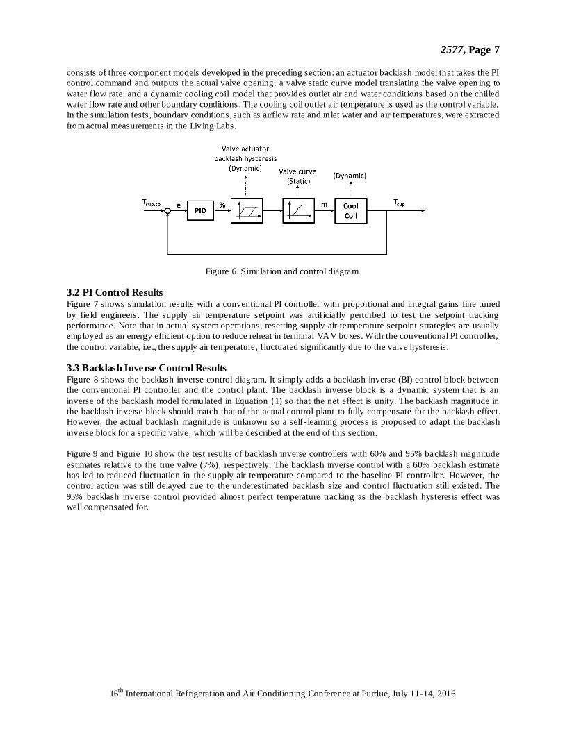
3.1 Simulation Test Setup An emulator model was constructed by combining the valve and cooling coil models developed in the preceding
section. Figure 6 shows the component layout of the emulator models along with the feedback control loop. For
typical cooling coil operation, a feedback controller, e.g., a PI controller, is used to generate control commands for
the valve actuator to adjust valve opening so that the supply air temperature fo llows the setpoint. The emulator
2577, Page 7
16th
International Refrigerat ion and Air Conditioning Conference at Purdue, Ju ly 11-14, 2016
consists of three component models developed in the preceding section: an actuator backlash model that takes the PI
control command and outputs the actual valve opening; a valve static curve model translating the valve open ing to
water flow rate; and a dynamic cooling coil model that provides outlet air and water condit ions based on the chilled
water flow rate and other boundary conditions . The cooling coil outlet air temperature is used as the control variable.
In the simulation tests, boundary conditions, such as airflow rate and in let water and air temperatures, were extracted
from actual measurements in the Liv ing Labs.
Figure 6. Simulat ion and control diagram.
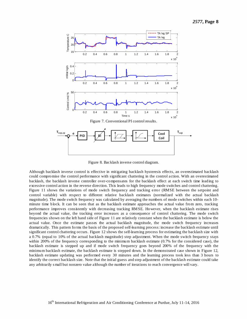
3.2 PI Control Results Figure 7 shows simulat ion results with a conventional PI controller with proportional and integral gains fine tuned
by field engineers. The supply air temperature setpoint was artificially perturbed to test the setpoint tracking
performance. Note that in actual system operations, resetting supply air temperature setpoint strategies are usually
employed as an energy efficient option to reduce reheat in terminal VAV boxes. With the conventional PI controller,
the control variable, i.e ., the supply air temperature, fluctuated significantly due to the valve hysteresis.
3.3 Backlash Inverse Control Results Figure 8 shows the backlash inverse control diagram. It simply adds a backlash inverse (BI) control b lock between
the conventional PI controller and the control plant. The backlash inverse block is a dynamic system that is an
inverse of the backlash model formulated in Equation (1) so that the net effect is unity. The backlash magnitude in
the backlash inverse block should match that of the actual control plant to fully compensate for the backlash effect.
However, the actual backlash magnitude is unknown so a self -learning process is proposed to adapt the backlash
inverse block for a specific valve, which will be described at the end of this section.
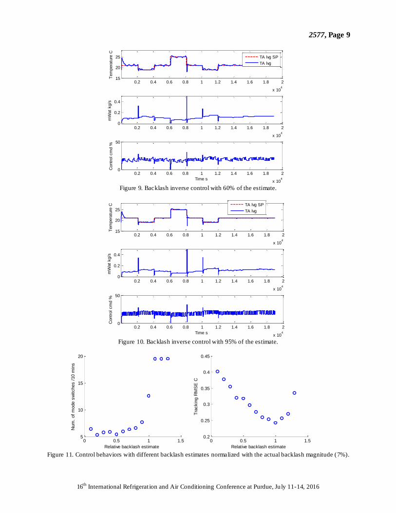
Figure 9 and Figure 10 show the test results of backlash inverse controllers with 60% and 95% backlash magnitude
estimates relat ive to the true valve (7%), respectively. The backlash inverse control with a 60% backlash estimate
has led to reduced fluctuation in the supply air temperature compared to the baseline PI controller. However, the
control action was still delayed due to the underestimated backlash size and control fluctuation still existed. The
95% backlash inverse control provided almost perfect temperature tracking as the backlash hysteresis effect was
well compensated for.
2577, Page 8
16th
International Refrigerat ion and Air Conditioning Conference at Purdue, Ju ly 11-14, 2016
0.2 0.4 0.6 0.8 1 1.2 1.4 1.6 1.8 2
x 104
15
20
25
Tem
pera
ture
C
TA lvg SP
TA lvg
0.2 0.4 0.6 0.8 1 1.2 1.4 1.6 1.8 2
x 104
0
0.2
0.4m
Wat
kg/s
0.2 0.4 0.6 0.8 1 1.2 1.4 1.6 1.8 2
x 104
0
50
Contr
ol cm
d %
Time s
Figure 7. Conventional PI control results.
Figure 8. Backlash inverse control diagram.
Although backlash inverse control is effect ive in mit igating backlash hysteresis effects, an overestimated backlash
could compromise the control performance with significant chattering in the control action. With an overestimated
backlash, the backlash inverse controller over-compensates for the backlash effect at each switch time lead ing to
excessive control action in the reverse direction. Th is leads to high frequency mode switches and control chattering.
Figure 11 shows the variations of mode switch frequency and tracking erro r (RMSE between the setpoint and
control variable) with respect to different relative backlash estimates (normalized with the actual backlash
magnitude). The mode switch frequency was calculated by averaging the numbers of mode switches within each 10-
minute time b lock. It can be seen that as the backlash estimate approaches the actual value from zero, tracking
performance improves consistently with decreasing tracking RMSE. However, when the backlash estimate rises
beyond the actual value, the tracking error increases as a consequence of control chattering. The mode switch
frequencies shown on the left hand side of Figure 11 are relatively constant when the backlash estimate is below the
actual value. Once the estimate passes the actual backlash magnitude, the mode switch frequency increases
dramat ically. This pattern fo rms the basis of the proposed self-learning process: increase the backlash estimate until
significant control chattering occurs. Figure 12 shows the self-learn ing process for estimating the backlash size with
a 0.7% (equal to 10% of the actual backlash magnitude) step adjustment. When the mode switch frequency stays
within 200% of the frequency corresponding to the minimum backlash estimate (0.7% for the considered case), the
backlash estimate is stepped up and if mode switch frequency goes beyond 200% of the frequency with the
minimum backlash estimate, the backlash estimate is stepped down. In the demonstrated case shown in Figure 12,
backlash estimate updating was performed every 30 minutes and the learning process took less than 3 hours to
identify the correct backlash size. Note that the init ial guess and step adjustment of the backlash estimate could take
any arbitrarily s mall but nonzero value although the number of iterat ions to reach convergence will vary.
2577, Page 9
16th
International Refrigerat ion and Air Conditioning Conference at Purdue, Ju ly 11-14, 2016
0.2 0.4 0.6 0.8 1 1.2 1.4 1.6 1.8 2
x 104
15
20
25
Tem
pera
ture
C
TA lvg SP
TA lvg
0.2 0.4 0.6 0.8 1 1.2 1.4 1.6 1.8 2
x 104
0
0.2
0.4
mW
at
kg/s
0.2 0.4 0.6 0.8 1 1.2 1.4 1.6 1.8 2
x 104
0
50
Contr
ol cm
d %
Time s
Figure 9. Backlash inverse control with 60% of the estimate.
0.2 0.4 0.6 0.8 1 1.2 1.4 1.6 1.8 2
x 104
15
20
25
Tem
pera
ture
C
TA lvg SP
TA lvg
0.2 0.4 0.6 0.8 1 1.2 1.4 1.6 1.8 2
x 104
0
0.2
0.4
mW
at
kg/s
0.2 0.4 0.6 0.8 1 1.2 1.4 1.6 1.8 2
x 104
0
50
Contr
ol cm
d %
Time s
Figure 10. Backlash inverse control with 95% of the estimate.
0 0.5 1 1.55
10
15
20
Relative backlash estimate
Num
. of
mode s
witches /
10 m
ins
0 0.5 1 1.50.2
0.25
0.3
0.35
0.4
0.45
Relative backlash estimate
Tra
ckin
g R
MS
E C
Figure 11. Control behaviors with different backlash estimates normalized with the actual backlash magnitude (7%).

2577, Page 10
16th
International Refrigerat ion and Air Conditioning Conference at Purdue, Ju ly 11-14, 2016
0.2 0.4 0.6 0.8 1 1.2 1.4 1.6 1.8 2
x 104
15
20
25
Tem
pera
ture
C
TA lvg SP
TA lvg
0.2 0.4 0.6 0.8 1 1.2 1.4 1.6 1.8 2
x 104
0
0.2
0.4m
Wat
kg/s
0.2 0.4 0.6 0.8 1 1.2 1.4 1.6 1.8 2
x 104
0
50
Contr
ol cm
d %
0.2 0.4 0.6 0.8 1 1.2 1.4 1.6 1.8 2
x 104
0
0.5
1
Backla
shE
st
Time s
Figure 12. Self-learning process to estimate the backlash size.
6. CONCLUSIONS
This paper proposed a self-learn ing backlash inverse control approach to mitigate the backlash hysteresis effects
associated with typical hydronic valves and to improve control performance. A specific HVAC application was
considered as a case study that applied the proposed backlash inverse control approach to a cooling coil valve. To
assess the control performance improvement, an emulator was constructed combin ing dynamic models of an
actuator (backlash effect) and a cooling coil calib rated with field measurements obtained from Living Labs at
Purdue. Simulation test results showed that for valves with noticeable backlash hys teresis, a conventional PI
controller led to low frequency fluctuations in the supply air temperature (control variable). The proposed backla sh
inverse control added to a conventional PI controller demonstrated significantly improved control performance in
mitigating the backlash effects and the best performance was achieved when the backlash size estimate was equal to
or slightly less than the actual valve backlash. Intensive control chattering occurs when the backlash size is
overestimated so a self-learning process was proposed that increments the backlash estimate from zero until
significant chattering occurs. Th is self-learn ing process was tested within the emulator model and the actual
backlash size was identified within three hours of operation.
The proposed backlash inverse control approach was also tested in the actual cooling coil operation serving the
Living Labs. The experimental testing results showed a close match with the simulat ion results under both baseline
and backlash inverse controls. However, the measurement noise in the experimental test induced severe mode
switches. This issue was previously reported by Dean et al. (1995) where a backlash inverse controller was applied
and tested within a servomotor. To overcome this issue, a buffered backlash inverse controller was proposed and the
testing results showed significantly improved control performance with moderate mode switches . Due to space
limitat ions, the buffered backlash inverse controller and the experimental testing results will be reported in future
publications.
NOMENCLATURE
cmd control command (%)
xBL backlash magnitude (-)
α backlash curve slope (-)
2577, Page 11
16th
International Refrigerat ion and Air Conditioning Conference at Purdue, Ju ly 11-14, 2016
x backlash state (-)
m mass/volumetric flow rate (kg/s or l/s)
open valve opening (%)
t time index (-)
T temperature (K)
cp specific heat at constant pressure (kJ/kg-K)
h enthalpy (kJ/kg)
R thermal resistance (K/W)
C thermal capacitance (kJ/K)
є effectiveness (-)
Tsup/Tlvg AHU supply air temperature (K)
Subscript
a air
w water
c coil material
sp setpoint
max maximum
Superscript
i the i-th control volume
* heat and mass transfer
REFERENCES
Ahmad, N. J., and Khorrami, F., "Adaptive control of systems with backlash hysteresis at the input." American
Control Conference, 1999.
ASHRAE. ASHRAE Handbook- HVAC Systems and Equipment, 2012.
Cai, J., Kurtulus O. and Braun, J.E., " Experimental performance investigation of cooling or heating coil valves and
their impact on temperature controls", 16th International Refrigeration and Air Conditioning Conference at
Purdue, 2016.
Dean, S.R., Surgenor, B.W. and Iordanou, H.N., "Experimental evaluation of a backlash inverter as applied to a
servomotor with gear t rain." IEEE Conference on Control Applications, 1995.
Hägglund, Tore. "Automatic on-line estimat ion of backlash in control loops." Journal of Process Control, 2007.
Kumar, V. and Mittal, A.P., "Dynamic modeling of liquid-flow process due to hysteresis of pneumatic control
valve", International Journal of Intelligent Control and Systems, 2010
Madsen, K., Nielsen, H.B. and Tingleff, O., Methods for Nonlinear Least Squares Problems, Informatics and
Mathematical Modeling, Technical University of Denmark, 2004.
Tao G. and P. Kokotovic. "Adaptive control of systems with backlash". Automatica, 1993
Tao G. and P. Kokotovic, Adaptive Control of Systems with Actuator and Sensor Nonlinearities , John Wiley &
sons, 1996
Tudoroiu, N., and M. Zaheeruddin, "Fault detection and diagnosis of valve actuators in HVAC systems." IEEE
Conference on Control Applications, 2005.
Zhou, X., Dynamic modeling of chilled water cooling coils, Ph.D. d issertation, Purdue University, 2005.