self-enforcing debt limits and costly default in general ... · sao paulo school of economics,...
TRANSCRIPT
Self-enforcing Debt Limits and Costly Default
in General Equilibrium
V. Filipe Martins-da-Rocha Toan Phan Yiannis Vailakis∗
December 5, 2017(Preliminary and incomplete. Click here for the latest version.)
Abstract
We establish a novel determination of self-enforcing debt limits at the
present value of default cost in a general competitive equilibrium. Agents can
trade state-contingent debt but cannot commit to repay. If an agent defaults,
she loses a fraction of her current and future endowments. Moreover, she is
excluded from borrowing but is still allowed to save, as in Bulow and Rogoff
(1989). Competition implies that debt limits are not-too-tight, as in Alvarez
and Jermann (2000). Under a mild condition that the endowment loss from
default is bounded away from zero, we show that the equilibrium interest rates
must be sufficiently high that the present value of aggregate endowments is
finite. We show that equilibrium debt limits are exactly equal to the present
value of endowment loss due to default. The determination of competitive debt
limits based on endowment loss is isomorphic to the determination of public
debt sustainable by tax revenues. We also show that competitive equilibria with
∗Sao Paulo School of Economics, Getulio Vargas Foundation (FGV) and CNRS; [email protected]. The Federal Reserve Bank of Richmond and the University of North Carolinaat Chapel Hill; [email protected]. The University of Glasgow; [email protected] thank Kartik Athreya, Guido Lorenzoni, Pietro Peretto, Nico Trachter, and various semi-nar/conference participatants at the Federal Reserve Bank of Richmond, Virginia Tech, Duke Uni-versity Triangle Dynamic Macro workshop, University of Tokyo, University of California Santa Cruzand Santa Clara University for useful comments and suggestions. The views expressed herein arethose of the authors and not those of the Federal Reserve Bank of Richmond or the Federal ReserveSystem.
1
self-enforcingdebt and costly default are equivalent to Arrow-Debreu equilibria
with limitedpledgeability, as defined by Gottardi and Kubler (2015).
1 Introduction
This paper addresses a classic question in macroeconomics: how much debt can
be sustained if borrowers cannot commit to repay? We develop a general equilibrium
model of risk sharing under multilateral lack of commitment. Agents would like to
borrow and lend to hedge against heterogeneous shocks to their endowments. If a
borrower defaults, the assumption is that she is excluded from borrowing but is still
allowed to save, as in Bulow and Rogoff (1989) and Hellwig and Lorenzoni (2009).
Competition implies that the endogenous debt limits must be not too tight, i.e., they
must be set at the largest possible levels such that repayment is individually rational,
as in Alvarez and Jermann (2000). A key departure is that, in addition to credit ex-
clusion, defaulting agents lose a fraction of their current and future endowments. This
assumption is relevant in the context of sovereign default, as it has been documented
that countries tend to suffer economic contractions during default episodes.1
Within this framework, we establish strong characteristics of the joint behavior of
the equilibrium interest rates (or intertemporal prices) and endogenous debt limits.
Under a mild condition on primitives, asserting that the total endowment loss across
agents is non-negligible (but the loss can be arbitrarily small and can flexibly vary
across agents and time), we provide a non-trivial insight about the forces that pin
down the implied interest rates and debt limits in a competitive equilibrium.
First, the interest rates must be sufficiently high such that the present value of
endowments across all agents in the economy is finite. As a consequent, there cannot
exist bubbly equilibria where debt is indefinitely rolled over. Second, it is endogenous
in equilibrium that the debt limits of any agent must not exceed the present value of
her endowments (the natural debt limit). Based on these two results, we establish the
1See, e.g., Trebesch et al. (2012), Tomz and Wright (2013), and Aguiar et al. (2014) for surveysof recent empirical research in the sovereign debt literature.
third, which states that the debt limits in any competitive equilibrium must exactly
be equal to the present value of endowment loss. This is not a mere coincidence,
as the determination of not-too-tight debt limits is akin to the pricing of assets in a
competitive equilibrium. The intuition is as follows. On the one hand, high implied
interest rates rule out the possibility that borrowers can indefinitely roll over their debt
as a Ponzi scheme. Therefore, equilibrium debt limits cannot exceed the present value
of output loss, as in Bulow and Rogoff (1989). On the other hand, in the presence
of direct costs, debtors would always choose to honour any debt not exceeding the
present value of pledgeable resources. Together, those forces imply that equilibrium
debt limits should exactly reflect the present value of output loss.
The argument above resembles the no-arbitrage argument that determines the
prices of long-lived assets, such as a Lucas tree, to the present value of the streams of
dividends, in any non-bubbly equilibrium under full commitment. In our environment
with limited commitment, the not-too-tight debt limits reflect the opportunity cost
of honouring the contractual arrangements of contingent debt, which is akin to the
value of a claim to debtors’ resources that would be lost due to default.
The results also provide an insight to an isomorphism between private debt and
public debt. We map the current model to an environment where agents cannot
issue debt; however, they can instead purchase public debt that is issued by a fiscal
authority. We show that as long as the authority can impose a non-negligible tax rate
on private agent endowments, the equilibrium interest rates are sufficiently high such
that bubbly equilibria, where the authority can indefinitely roll over debt, cannot
arise. Moreover, in any competitive equilibrium, the amount of public debt bought
by private agents must be exactly equal to the present value of tax revenues, i.e.,
public debt must be fully backed by taxation. This result stands in a stark contrast
to that in Hellwig and Lorenzoni (2009), where the authors show that in the absence
of any tax base, any positive amount of public debt in equilibrium must be indefinitely
rolled over as a bubble. Our result thus points to the fragility of bubbly equilibria,
in a similar sense that the presence of a Lucas tree with non-vanishing dividends can
rule out the possibility of rational bubbles (see Santos and Woodford, 1997 and also
3

Tirole, 1985).
Our general equilibrium model also nests the partial equilibrium model of Bulow
and Rogoff (1989) (henceforth BR) as a special case, and our results imply as a
corollary their celebrated debt impossibility theorem. They show that, if (i) the
interest rates are such that present value of endowments of an agent (or country) is
finite, and (ii) the agent’s borrowing cannot exceed the natural debt limit, then it
is impossible to sustain positive borrowing when the only punishment for default is
exclusion from future credit. A key difference is that while BR impose assumptions
(i) and (ii) on endogenous variables (equilibrium prices and quantities), these two
properties arise naturally in our environment.
From a technical standpoint, our proofs exploit a new characterization of not-too-
tight debt limits that can be of independent interest. The interesting feature of our
characterization result, which has no analogue in the absence of output costs, is its
implication about the level of interest rates. As stressed above, we do not impose a
priori any restriction on interest rates. We instead show that no matter how small
is the output loss, interest rates must be higher than agents’ growth rates if debt is
self-enforcing. This, in turn, allows us to show that any process of self-enforcing debt
limits is the sum of the present value of output losses and a “bubble” component.
Taking into account market clearing conditions, at equilibrium, the self-enforcing debt
limits coincide with the present value of output losses (i.e., equilibrium debt limits
are bubble free).
Related literature. Our paper is closely related to the general equilibrium models of
risk sharing with limited commitment and endogenous borrowing constraints. Kehoe
and Levine (1993), Kocherlakota (1996), Alvarez and Jermann (2000, 2001), and
Kehoe and Perri (2004) develop models where agents are excluded from financial
markets after default, while Hellwig and Lorenzoni (2009) and Martins-da-Rocha and
Vailakis (2016, 2017) develop models where defaulters are only excluded from future
credit, as in BR.2 To the best of our knowledge, our paper is the first to introduce
2See also Kletzer and Wright (2000) for a game theoretic analysis of the threat of credit exclusion.
4

recourse or endowment loss from default into this general equilibrium environment.
From a substantive point of view, while most existing papers impose assumptions
on endogenous variables, namely the equilibrium interest rates are high and/or the
debt limits are bounded by wealth, the introduction of the default loss allows us to
generate these properties endogenously.
Our paper is also related to the rational bubbles literature (Diamond, 1965, Tirole,
1985, Miao and Wang, 2011, Farhi and Tirole, 2012, Martin and Ventura, 2012, Hirano
and Yanagawa, 2016) and papers on the shortage of assets (Caballero et al., 2008,
J. Caballero and Farhi, 2017). A common theme of these papers is that a shortage
of savings instruments or a shortage of collateral depresses the interest rates, raising
the present value of aggregate output or endowments, leading to the possibility of
rational bubbles. Our paper shows that the introduction of arbitrarily small but non-
negligible endowment loss from default guarantees finite wealth and rules out the
possibility of bubbles. Thus, our paper complements Santos and Woodford (1997) in
highlighting the fragility of the conditions for the existence of bubbles.
Finally, our paper is also related to Woodford (1990) and Holmstrom and Tirole
(1998, 2011) in highlighting the relationship between private liquidity and public
liquidity in environments with financial frictions that lead to scarce collateral.
2 Environment
2.1 Uncertainty
Time and uncertainty are both discrete. We use an event tree Σ to describe time,
uncertainty and the revelation of information over an infinite horizon. There is a
unique initial date-0 event s0 ∈ Σ and for each date t ∈ {0, 1, 2, . . .} there is a finite set
St ⊆ Σ of date-t events st. Each st has a unique predecessor σ(st) in St−1 and a finite
number of successors st+1 in St+1 for which σ(st+1) = st. We use the notation st+1 � st
to specify that st+1 is a successor of st. Event st+τ is said to follow event st, also
denoted st+τ � st, if σ(τ)(st+τ ) = st. The set St+τ (st) := {st+τ ∈ St+τ : st+τ � st}
5

denotes the collection of all date-(t+τ) events following st. Abusing notation, we let
St(st) := {st}. The subtree of all events starting from st is then
Σ(st) :=⋃τ≥0
St+τ (st).
We use the notation sτ � st when sτ � st or sτ = st. In particular, we have
Σ(st) = {sτ ∈ Σ : sτ � st}.
2.2 Endowments and Preferences
There is a single perishable consumption good, and the economy consists of a
finite set I of household types, each type consists of a unit measure of identical
agents. Agents are infinitely lived. They cannot commit to future actions.
The preferences of agents over (non-negative) consumption processes c = (c(st))st∈Σ
are represented by the lifetime expected and discounted utility functional
U(c) :=∑t≥0
βt∑st∈St
π(st)u(c(st))
where β ∈ (0, 1) is the discount factor, π(st) is the unconditional probability of st and
u : R+ → [−∞,∞) is a Bernoulli function assumed to be strictly increasing, concave,
continuous on R+, differentiable on (0,∞), bounded and satisfying Inada’s condition
at the origin.3 Given an event st, we denote by U(c|st) the lifetime continuation
utility conditional to st defined by
U(c|st) := u(c(st)) +∑τ≥1
βτ∑
st+τ�stπ(st+τ |st)u(c(st+τ ))
3The function u is said to satisfy the Inada’s condition at the origin if limε→0[u(ε)−u(0)]/ε =∞.We assume that agents’ preferences are homogeneous. This is only for the sake of simplicity. Allarguments can be adapted to handle the heterogeneous case where the preferences differ amongagents. The boundedness of u is only used to establish a necessary condition of the equilibriumdebt limits. It can be relaxed if we impose some mild restrictions on the endowments and defaultpunishment. We refer to Remark 1 for the detailed discussion.
6

where π(st+τ |st) := π(st+τ )/π(st) is the conditional probability of st+τ given st.
Agents receive endowments in each period that are subject to random shocks.
We denote by yi = (yi(st))st∈Σ the process of positive endowments yi(st) > 0 of the
representative agent of type i.4 A collection (ci)i∈I of consumption processes is called
a consumption allocation. It is said to be resource feasible if∑
i∈I ci =
∑i∈I y
i. We
also fix an allocation (ai(s0))i∈I of initial financial claims ai(s0) ∈ R that satisfies the
usual market clearing condition:∑
i∈I ai(s0) = 0. The initial financial claim ai(s0)
can be interpreted the consequence of (un-modeled) past transactions.
2.3 Markets
At any event st, agents can issue and trade a complete set of one-period contingent
bonds which promise to pay one unit of the consumption good contingent on the
realization of any successor event st+1 � st. Let q(st+1) > 0 denote the price at
event st of the st+1-contingent bond. Agent i’s holding of this bond is ai(st+1).
The amount of state-contingent debt agent i can issue is observable and subject to
state-contingent (non-negative and finite) debt limits Di = (Di(st))st∈Σ. Given the
initial financial claim ai(s0), we denote by Bi(Di, ai(s0)) the budget set of an agent
who never defaults. It consists of all pairs (ci, ai) of consumption and bond holdings
satisfying the following constraints: for any event st,
ci(st) +∑
st+1�stq(st+1)ai(st+1) ≤ yi(st) + ai(st) (2.1)
and
ai(st+1) ≥ −Di(st+1), for all st+1 � st. (2.2)
Fix an event sτ and some initial claim a ∈ R. We denote by V i(Di, a|sτ ) the value
function defined by
V i(Di, a|sτ ) := sup{U(ci|sτ ) : (ci, ai) ∈ Bi(Di, a|sτ )}4For brevity, instead of saying “the representative agent of type i”, we simply say “agent i” in
the remaining of the paper.
7

where Bi(Di, a|sτ ) is the set of all plans (ci, ai) satisfying ai(sτ ) = a together with
restrictions (2.1) and (2.2) at every successor node st � sτ .
Without any loss of generality, we restrict attention to debt limits (Di(st))st�s0
that are consistent, meaning that at every event st, the maximal debt can be repaid
out of the current resources and the largest possible debt contingent on future events,
i.e.,
Di(st) ≤ yi(st) +∑
st+1�stq(st+1)D(st+1), for all st � s0. (2.3)
The above condition is necessary for the budget set Bi(Di,−Di(st)|st) to be non-
empty.5
2.4 Default Costs
An agent might not honor her debt obligations and decide to default if it is optimal
for her. The decision to default depends on the consequences of default. As in Bulow
and Rogoff (1989), we assume that defaulters start with neither assets nor liabilities,
are excluded from future credit, but retain the ability to purchase bonds. In addition,
they suffer a (possibly zero) fractional loss in income upon default.6 Specifically, debt
repudiation leads to a contraction τ i(st) ∈ [0, 1] of agent i’s endowment, where τ may
vary across agents and events. Formally, agent i’s default option at event st is the
largest continuation utility when starting with zero financial claims, cannot borrow
and her income reduces by a fraction τ i(sτ ) at every sτ � st:
V id (0, 0|st) := sup{U(ci|st) : (ci, ai) ∈ Bi
d(0, 0|st)}, (2.4)
5It is straightforward to check that any process of self-enforcing debt limits (defined in Sec-tion 2.5) and any process of natural debt limits (defined in Section 2.6) satisfies the consistencyproperty (2.3).
6Disruption of international trade or of the domestic financial system can lead to output dropsif either trade or banking credit is essential for production. Among others, Mendoza and Yue(2012), Gennaioli et al. (2014), and Phan (2017) model explicitly how sovereign default may leadto an efficiency loss in production. We follow the tradition in the sovereign debt literature (see forinstance Cohen and Sachs (1986), Cole and Kehoe (2000), Aguiar and Gopinath (2006), Arellano(2008), Abraham and Carceles-Poveda (2010), and Bai and Zhang (2010, 2012)) and model thenegative implications on output by the loss of an exogenous fraction of income.
8

where Bid(0, 0|st) denotes the budget set corresponding to Bi(0, 0|st) when the en-
dowment yi(sτ ) is replaced by (1− τ i(sτ ))yi(sτ ) at any event sτ � st.
Remark 1. We have assumed that the Bernoulli function u is bounded. This assump-
tion can be dropped if the primitives of the economy satisfy the following properties:
(a) the default option V id (0, 0|st) is finite for all agent i and event st;
(b) If a resource feasible consumption allocation (ci)i∈I satisfies the participation
constraints U(ci|st) ≥ V id (0, 0|st) for all agent i and event st, then the continuation
utility U(ci|st) is finite for all agent i and event st.7
The above conditions are obviously true when the Bernoulli function is bounded.
However, they are also satisfied if for all agent i and every event st we have
−∞ < U((1− τ i)yi|st) and U(y|st) <∞,
where y :=∑
i∈I yi is the aggregate endowment. The above inequalities are valid
if the endowments are uniformly bounded from above and away from zero and the
contraction coefficients (τ i)i∈I are uniformly bounded away from 1.
2.5 Self-enforcing Debt Limits
We now incorporate the fact that agents have the option to default. Since bor-
rowers issue contingent bonds, lenders have no incentives to provide credit contingent
to some event if they anticipate that a debtor will default.8 The maximum amount
of debt Di(st) at any event st � s0 should reflect this property. If agent i’s ini-
tial financial claim at event st corresponds to the maximum debt −Di(st), then she
prefers to repay her debt if, and only if, V i(Di,−Di(st)|st) ≥ V id (0, 0|st). When a
process of bounds satisfies the above inequality at every node st � s0, it is called
7Observe that any consumption allocation derived from a competitive equilibrium (defined inSection 4) necessarily satisfies the participation constraints.
8Since the default punishment is independent of the default level, there is no partial default.Agents either repay or default totally.
9

self-enforcing.9 Competition among lenders naturally leads to consider the largest
self-enforcing bound Di(st) defined by the equation
V i(Di,−Di(st)|st) = V id (0, 0|st). (2.5)
We follow Alvarez and Jermann (2000) and refer to such debt limits as not-too-tight.
Remark 2. If we fix an agent i and assume that τ i(st) = 1 for all every event st,
then the agent has no incentive to ever default. Equivalently, in this case, the agent
can effectively commit to her financial promises. This is because the value of the
default option is V id (0, 0|st) = U(0|st), and consequently any process of consistent
debt limits is self-enforcing. Therefore, the specification of output costs encompasses
a mixed environment where some agents can perfectly commit to financial contracts
while others have limited commitment.10 In case where τ i(st) = 1 for all event st and
agent i, the model collapses to a standard risk-sharing model with full commitment.
2.6 Natural Debt Limits
Given state-contingent bond prices q = (q(st))st�s0 , we denote by p(st) the as-
sociated date-0 price of consumption at st defined recursively by p(s0) = 1 and
p(st+1) = q(st+1)p(st) for all st+1 � st. We use PV(x|st) to denote the present
value at event st of a process x restricted to the subtree Σ(st) and defined by
PV(x|st) :=1
p(st)
∑st+τ∈Σ(st)
p(st+τ )x(st+τ ).
When the present value PV(yi|s0) is finite, we say that agent i has finite wealth11
9Indeed, since the function a 7→ V i(Di, a|st) is increasing, for any bond holding ai(st) satisfyingthe restriction ai(st) ≥ −Di(st), agent i prefers honouring her obligation than defaulting on ai(st).
10In particular, our model nests both the model in Bulow and Rogoff (1989) (unilateral lack ofcommitment) and the one in Hellwig and Lorenzoni (2009) (multilateral lack of commitment).
11Some authors use the terminology “interest rates are higher (respectively lower or equal) thanagent i’s growth rates” when the agent’s wealth is finite (respectively infinite). The choice of thisterminology is driven by the following particular case. Assume that interest rates and bounds
10
and define
W i(st) := PV(yi|st).
The process (W i(st))st∈Σ is called the process of natural debt limits. In a Arrow–
Debreu economy starting at event st, the limit W i(st) is the largest amount agent i
can consume at event st if she can commit to deliver all of her future resources and
consume zero forever. We say that a process of debt limits (Di(st))st�s0 is naturally
bounded when it is tighter than the natural debt limits, i.e., Di(st) ≤ W i(st) for all
event st.
3 Partial Equilibrium
This section presents a characterization of self-enforcing debt limits that can be
obtained as a corollary of the original results in Bulow and Rogoff (1989).12
They consider a partial equilibrium set up.13 The following result asserts that
equilibrium debt can only be sustained by the present value of endowment loss. In
the absence of endowment loss, debt cannot be sustained by the threat of credit
exclusion alone.
Lemma 1 (Bulow and Rogoff). Consider an arbitrary agent i constrained by a process
(Di(st))st�s0 of self-enforcing debt limits. Assume that
(i) prices are such that the agent’s wealth is finite, i.e., W i(s0) <∞, and
on growth rates are time and state invariant, i.e., q(st+1) = π(st+1|st)(1 + r)−1 and yi(st+1) =(1+gi(st+1))yi(st) for all st+1 � st, where the stochastic growth rate is such that migi ≤ gi(st+1) ≤M igi for some parameter gi with 0 < mi ≤ M i < ∞. Then, the agent i’s wealth is finite if, andonly if, r > gi, and infinite if, and only if, r ≤ gi.
12We refer to Martins-da-Rocha and Vailakis (2016) for the detailed connection. Here we onlyremark that the model in Bulow and Rogoff (1989) is slightly different than ours since they considera sovereign who trades at the initial node a complete set of state-contingent contracts that specifythe net transfers to foreign investors in all future periods and events. Contracts are restricted to becompatible with repayment incentives and allow investors to break even in present value terms (thisenvironment is in the spirit of Kehoe and Levine (1993) but with a different default option).
13A small open economy issues debt taking as given an exogenous, time-invariant world interestrate.
11

(ii) Di is naturally bounded, i.e., Di(st) ≤ W i(st) at every event st.
Then debt limits cannot exceed the present value of endowment loss:
Di(st) ≤ PV(τ iyi|st), for all st � s0.
In particular, if τ i = 0, then Di = 0, i.e., if there is no endowment loss, then debt is
not sustainable.
In a general equilibrium set up, conditions (i) and (ii) impose ad-hoc restrictions
on endogenous variables (prices and debt limits). A natural question that arises is
whether those restrictions hold true at a competitive equilibrium. A contribution
of this paper is to identify assumptions on primitives such that, at a competitive
equilibrium, the aggregate wealth of the economy is finite and the debt limits are
naturally bounded.
4 General Equilibrium
Instead of imposing conditions on endogenous variables (as prices and debt limits),
we now address the issue of debt sustainability in the context of a general equilibrium
setup.
Definition 1. For given initial asset positions ai(s0) such that∑
i∈I ai(s0) = 0,
a competitive equilibrium with self-enforcing debt (q, (ci, ai, Di)i∈I) consists of state-
contingent bond prices q, a resource feasible consumption allocation (ci)i∈I , a market
clearing allocation of bond holdings (ai)i∈I and an allocation of consistent and finite
debt limits (Di)i∈I such that:
(a) for each agent i ∈ I, taking prices and the debt limits as given, the plan (ci, ai)
is optimal among budget feasible plans in Bi(Di, ai(s0)|s0);
(b) for each agent i ∈ I, the sequence of debt limits Di are not-too-tight, i.e., equa-
tion (2.5) is satisfied at all events.
12

Our first result establishes a lower bound on equilibrium debt limits:
Lemma 2. Not-too-tight debt limits are at least as large as the present value of
endowment loss: Di(st) ≥ PV(τ iyi|st) for each event st and each agent i.
This result provides an intuitive lower bound on equilibrium debt limits, which
must be not-too-tight, and serves as an important result for the analysis in the
remaining of the paper. A natural approach to prove this result is to show that
Di(st) ≥ τ i(st)yi(st) + Di(st) where Di(st) :=∑
st+1�st q(st+1)Di(st+1) is the present
value of next period’s debt limits, and then use a standard iteration argument.
Because in equilibrium, debt limits are not-too-tight, this is equivalent to proving
that agent i does not have an incentive to default when her net asset position is
τ i(st)yi(st) + Di(st), i.e.,
V i(Di,−τ i(st)yi(st)− Di(st)|st) ≥ V id (0, 0|st). (4.1)
By definition, the default value function V id satisfies:
V id (0, 0|st) ≥ u((1− τ i(st))yi(st)) + β
∑st+1�st
π(st+1|st)V id (0, 0|st+1). (4.2)
If we had an equality in (4.2), then inequality (4.1) would be straightforward. Indeed,
consuming (1− τ i(st))yi(st) and borrowing up to each debt limit Di(st+1) at event st
leads to the right hand side continuation utility in (4.2), and satisfies the solvency
constraint at event st in the budget set defining the left hand side of (4.1). However, in
our environment where an agent can save upon default, (4.2) need not be satisfied with
an equality.14 Dealing with this problem is non-trivial and constitutes the technical
contribution in the proof presented in Appendix A.1.
14In the simpler environment where saving is not possible after default (as it is the case in Alvarezand Jermann (2000)) we always have an equality in (4.2).
13

4.1 Wealth must be finite
From now on we impose the following minimal assumption on the structure of
endowment loss:
Assumption 1. The aggregate endowment loss from default is non-negligible (with
respect to aggregate endowments), in the sense that there exists ε > 0 such that:∑i∈I
τ i(st)yi(st) ≥ ε∑i∈I
yi(st), for all st � s0. (4.3)
The above property is satisfied, for example, if the fraction of endowment loss
is uniformly positive for all agents, i.e., for all agent i ∈ I, there exists ε > 0 such
that τ i(st) ≥ ε at any event st ∈ Σ. Moreover, the property is still satisfied even
if only a subset of agents face endowment loss. For example, assume a subset of
agents Ic ⊆ I (the “committed types”) face the maximum endowment loss: τ i = 1
for all i ∈ Ic; the remaining agents (the “uncommitted types”) do not face any
endowment loss: τ i = 0 for all i ∈ I \ Ic. Condition (4.3) still holds as long as the
total endowment of the committed types is non-negligible, i.e., there exists ε > 0 such
that∑
i∈Ic yi(st) ≥ ε
∑i∈I y
i(st).
The combination of Lemma 2 and Assumption 1 yields an important result about
equilibrium interest rates. The result states that no matter how small the output costs
are, as long as they are non-negligible, the present value of the stream of endowments
– discounted at the equilibrium interest rates – must be finite. More informally,
this result implies that the interest rates in any competitive equilibrium with non-
negligible endowment loss must be at least as high as the growth rate of the economy.
Theorem 1. Assume non-negligible endowment loss. In any competitive equilibrium
with self-enforcing debt, the wealth of any agent is finite, i.e., W i(s0) <∞ for all i ∈I. As a consequence, the aggregate wealth of the economy is finite, i.e.,
∑i∈IW
i(s0) <
∞.
14

Proof. Since the aggregate endowment loss is non-negligible (Assumption 1), we have∑i∈I
PV(τ iyi|s0) ≥ ε∑i∈I
PV(yi|s0) = ε∑i∈I
W i(s0).
On the other hand, Lemma 2 implies that∑i∈I
Di(s0) ≥∑i∈I
PV(τ iyi|s0).
Combining the two inequalities above yields the following inequality:∑i∈I
Di(s0) ≥ ε∑i∈I
W i(s0).
Since the debt limits Di are finite by definition, the inequality implies that the ag-
gregate wealth of the economy∑
i∈IWi(s0) is finite. As a corollary, each individual’s
wealth W i(s0) is finite.
This result stands in stark contrast with the result of Hellwig and Lorenzoni
(2009), which states that in the absence of endowment loss, any equilibrium with
positive debt requires low interest rates, so that each agent’s wealth is infinite. In
other words, the result state that if we introduce even just very small but non-
negligible endowment loss, we can effectively rule out bubbly equilibria. This fragility
of bubbly equilibria is related to Santos and Woodford (1997) and Tirole (1985), who
find that the existence conditions for bubbles are relatively fragile.
4.2 Equilibrium debt limits must be naturally bounded
Finite aggregate wealth implies the necessity of a market transversality condition
(see equation (4.4) below). This condition in turn allows us to show that the present
value of debt limits satisfies an asymptotic property (see 4.7 below). We then deduce
from the consistency property (2.3) that debt limits are bounded from above by
15
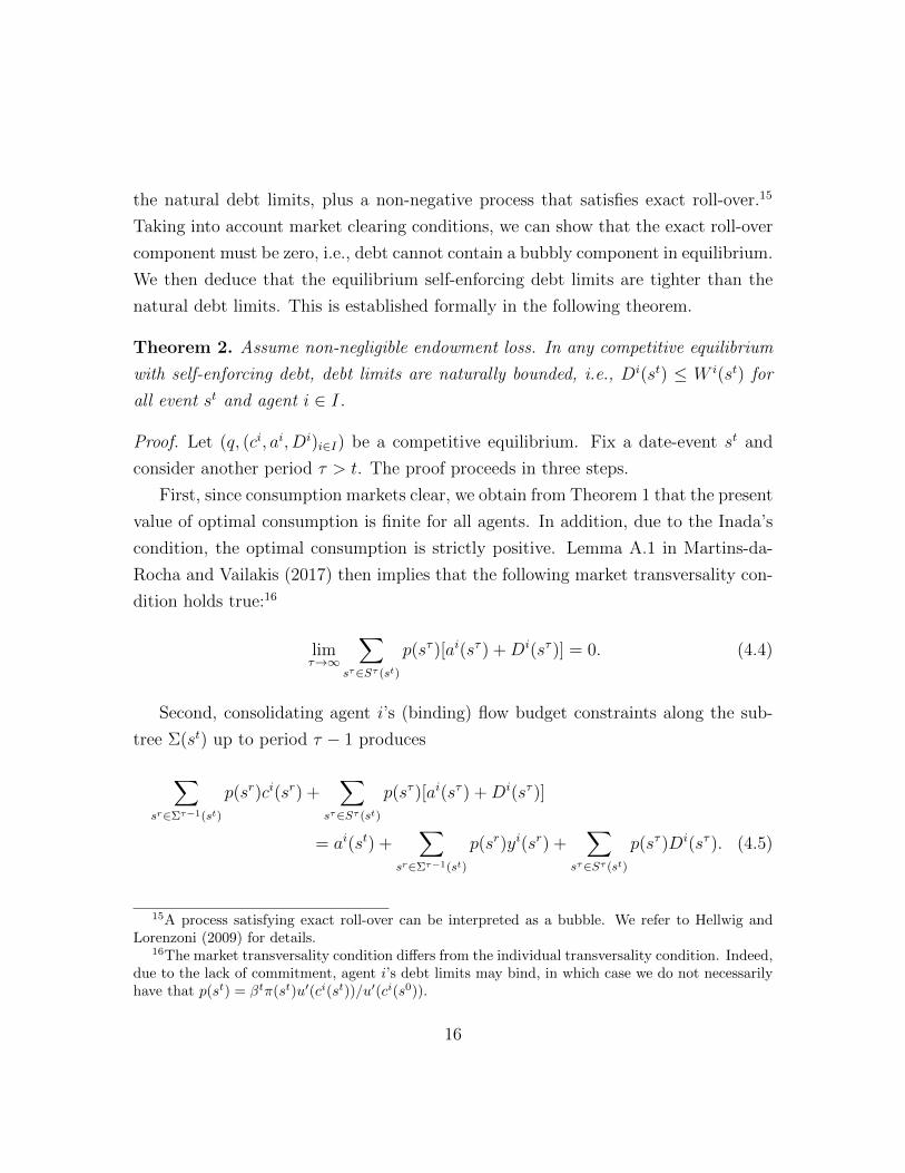
the natural debt limits, plus a non-negative process that satisfies exact roll-over.15
Taking into account market clearing conditions, we can show that the exact roll-over
component must be zero, i.e., debt cannot contain a bubbly component in equilibrium.
We then deduce that the equilibrium self-enforcing debt limits are tighter than the
natural debt limits. This is established formally in the following theorem.
Theorem 2. Assume non-negligible endowment loss. In any competitive equilibrium
with self-enforcing debt, debt limits are naturally bounded, i.e., Di(st) ≤ W i(st) for
all event st and agent i ∈ I.
Proof. Let (q, (ci, ai, Di)i∈I) be a competitive equilibrium. Fix a date-event st and
consider another period τ > t. The proof proceeds in three steps.
First, since consumption markets clear, we obtain from Theorem 1 that the present
value of optimal consumption is finite for all agents. In addition, due to the Inada’s
condition, the optimal consumption is strictly positive. Lemma A.1 in Martins-da-
Rocha and Vailakis (2017) then implies that the following market transversality con-
dition holds true:16
limτ→∞
∑sτ∈Sτ (st)
p(sτ )[ai(sτ ) +Di(sτ )] = 0. (4.4)
Second, consolidating agent i’s (binding) flow budget constraints along the sub-
tree Σ(st) up to period τ − 1 produces
∑sr∈Στ−1(st)
p(sr)ci(sr) +∑
sτ∈Sτ (st)
p(sτ )[ai(sτ ) +Di(sτ )]
= ai(st) +∑
sr∈Στ−1(st)
p(sr)yi(sr) +∑
sτ∈Sτ (st)
p(sτ )Di(sτ ). (4.5)
15A process satisfying exact roll-over can be interpreted as a bubble. We refer to Hellwig andLorenzoni (2009) for details.
16The market transversality condition differs from the individual transversality condition. Indeed,due to the lack of commitment, agent i’s debt limits may bind, in which case we do not necessarilyhave that p(st) = βtπ(st)u′(ci(st))/u′(ci(s0)).
16

By letting τ converge to infinity, transversality condition (4.4) and consolidated bud-
get equation (4.5) imply:
PV(ci|st) = ai(st) +W i(st) +M i(st), (4.6)
where:
M i(st) :=1
p(st)limτ→∞
∑sτ∈Sτ (st)
p(sτ )Di(sτ ) exists in R+. (4.7)
Observe that the process M i satisfies the following Martingale or exact-roll-over prop-
erty
∀st ∈ Σ, M i(st) =∑
st+1�stq(st+1)M i(st+1). (4.8)
Summing over i in equation (4.6) and exploiting market clearing implies that
∀st ∈ Σ,∑i∈I
M i(st) = 0.
Since each M i is non-negative we get that M i = 0 for all i ∈ I.
Finally, since the debt limits are consistent (i.e., they obey condition (2.3)), for
all arbitrary date-event st and every period τ > t, we have
p(st)Di(st) ≤τ∑r=t
∑st∈Sr(st)
p(sr)yi(sr) +∑
sτ∈Sτ (st)
p(sτ )Di(sτ ).
Passing to the limit when τ tends to infinite, we get that
Di(st) ≤ W i(st) +M i(st). (4.9)
Because M i = 0, inequality (4.9) then implies that Di ≤ W i for all agents.
Remark 3. If Assumption 1 is dropped, then Theorem 1 and Theorem 2 may fail. For
instance, if there is no output drop upon default, Hellwig and Lorenzoni (2009) provide
17

an example where, at a competitive equilibrium, each agent’s wealth is infinite. Even
if some agents can fully commit to honor their debt obligations, pledging all of their
income as collateral, the equilibrium debt limits of those agents may not be naturally
bounded. We refer to Appendix B for an example.
4.3 Exact characterization of equilibrium debt limits
Theorems 1 and 2 together with Lemma 1 allow us to have an exact character-
ization of the debt limits in equilibrium, without having to impose assumptions on
endogenous variables (the interest rates or debt limits). Specifically, because Theo-
rem 1 states that each agent’s wealth is finite and Theorem 2 states that each agent’s
debt limit is naturally bounded, both conditions (i) and (ii) in Lemma 1 are auto-
matically satisfied. This allows us to establish the following result:
Theorem 3. Assume non-negligible endowment loss. In any competitive equilibrium
with self-enforcing debt, the debt limit must be exactly equal to the present value of
endowment loss:
Di(st) = PV(τ iyi|st), for all st � s0. (4.10)
Proof. Theorems 1 and 2 imply that conditions (i) and (ii) of Lemma 1 are satisfied.
As a consequence, Lemma 1 implies that we have an upper bound on the debt limits:
Di(st) ≤ PV(τ iyi|st), for all st and every i.
On the other hand, from Lemma 2, we have a lower bound on the debt limits:
Di(st) ≥ PV(τ iyi|st), for all st and every i.
As the bounds coincide, it must be that equilibrium debt limits are exactly equal to
the present value of endowment loss, i.e., equation (4.10) holds.
This theorem formalizes a non-trivial insight. There are three forces that pin down
the debt limits in any competitive equilibrium. First, the presence of non-negligible
18

endowment loss implies that interest rates are sufficiently high that aggregate wealth
(and thus the present value of endowment loss) is finite. Second, the threat of default
and high interest rates imply that self-enforcing debt limits cannot exceed the present
value of endowment loss. Third, competition among lenders implies that debt limits
must be not too tight, which, in equilibrium, must be at least as large as the present
value of endowment loss. Together, they imply that equilibrium debt limits must
exactly coincide with the present value of endowment loss.
This theorem formalizes a non-trivial insight. There are four forces that pin down
the debt limits in any competitive equilibrium. First, competition among lenders
imply that debt limits must be not too tight, which, in equilibrium, must be at least
as large as the present value of endowment loss (Lemma 2). Second, the assumption
of non-negligible endowment loss implies that interest rates are sufficiently high that
aggregate wealth is finite (Theorem 1). Third, high interest rates and market clearing
imply that debt limits are naturally bounded (Theorem 2). Fourth, the possibility
to save after default imply that self-enforcing debt limits cannot exceed the present
value of endowment loss (Lemma 1). Together, they imply that equilibrium debt
limits must exactly coincide with the present value of endowment loss.
The theorem also generalizes (and strengthen) Bulow and Rogoff result to the
general equilibrium framework (without having to impose ad-hoc assumptions on
endogenous quantities and prices). It implies that as long as the endowment loss is
non-negligible, BR claim in Lemma 1 that Di ≤ PV(τ iyi) holds with equality. A
special case is the celebrated no-debt result:
Corollary 1. Assume non-negligible endowment loss. If an agent i faces no cost of
default (τ i = 0) then she cannot borrow in equilibrium (Di = 0).
5 Simple example
To clearly illustrate the main results of the paper, we turn to a special case of our
general environment.
Consider a deterministic economy with two agents I := {i1, i2}. The agents’
19
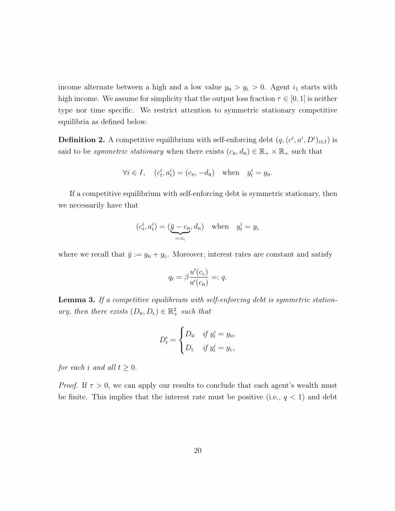
income alternate between a high and a low value yh > yl > 0. Agent i1 starts with
high income. We assume for simplicity that the output loss fraction τ ∈ [0, 1] is neither
type nor time specific. We restrict attention to symmetric stationary competitive
equilibria as defined below.
Definition 2. A competitive equilibrium with self-enforcing debt (q, (ci, ai, Di)i∈I) is
said to be symmetric stationary when there exists (ch, dh) ∈ R+ × R+ such that
∀i ∈ I, (cit, ait) = (ch,−dh) when yit = yh.
If a competitive equilibrium with self-enforcing debt is symmetric stationary, then
we necessarily have that
(cit, ait) = (y − ch︸ ︷︷ ︸
=:cl
, dh) when yit = yl
where we recall that y := yh + yl. Moreover, interest rates are constant and satisfy
qt = βu′(cl)
u′(ch)=: q.
Lemma 3. If a competitive equilibrium with self-enforcing debt is symmetric station-
ary, then there exists (Dh, Dl) ∈ R2+ such that
Dit =
Dh if yit = yh,
Dl if yit = yl,
for each i and all t ≥ 0.
Proof. If τ > 0, we can apply our results to conclude that each agent’s wealth must
be finite. This implies that the interest rate must be positive (i.e., q < 1) and debt
20
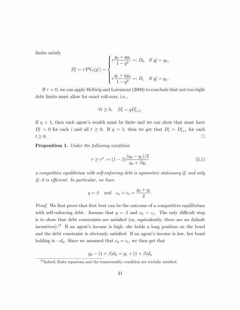
limits satisfy
Dit = τ PVt(y
i) =
τyh + qyl1− q2
=: Dh if yit = yh,
τyl + qyh1− q2
=: Dl if yit = yl.
If τ = 0, we can apply Hellwig and Lorenzoni (2009) to conclude that not-too-tight
debt limits must allow for exact roll-over, i.e.,
∀t ≥ 0, Dit = qDi
t+1.
If q < 1, then each agent’s wealth must be finite and we can show that must have
Dit = 0 for each i and all t ≥ 0. If q = 1, then we get that Di
t = Dit+1 for each
t ≥ 0.
Proposition 1. Under the following condition
τ ≥ τ ? := (1− β)(yh − yl)/2yh + βyl
(5.1)
a competitive equilibrium with self-enforcing debt is symmetric stationary if, and only
if, it is efficient. In particular, we have
q = β and ch = cl =yh + yl
2.
Proof. We first prove that first best can be the outcome of a competitive equilibrium
with self-enforcing debt. Assume that q = β and ch = cl. The only difficult step
is to show that debt constraints are satisfied (or, equivalently, there are no default
incentives).17 If an agent’s income is high, she holds a long position on the bond
and the debt constraint is obviously satisfied. If an agent’s income is low, her bond
holding is −dh. Since we assumed that ch = cl, we then get that
yh − (1 + β)dh = yl + (1 + β)dh
17Indeed, Euler equations and the transversality condition are trivially satisfied.
21
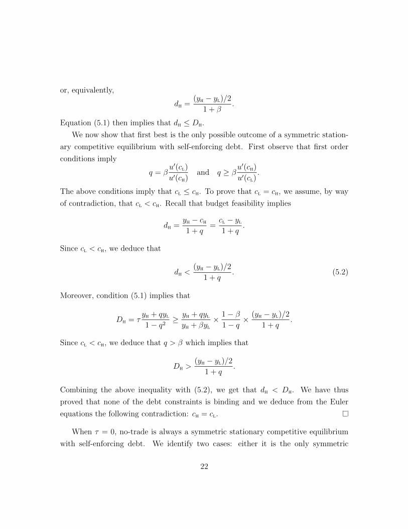
or, equivalently,
dh =(yh − yl)/2
1 + β.
Equation (5.1) then implies that dh ≤ Dh.
We now show that first best is the only possible outcome of a symmetric station-
ary competitive equilibrium with self-enforcing debt. First observe that first order
conditions imply
q = βu′(cl)
u′(ch)and q ≥ β
u′(ch)
u′(cl).
The above conditions imply that cl ≤ ch. To prove that cl = ch, we assume, by way
of contradiction, that cl < ch. Recall that budget feasibility implies
dh =yh − ch1 + q
=cl − yl1 + q
.
Since cl < ch, we deduce that
dh <(yh − yl)/2
1 + q. (5.2)
Moreover, condition (5.1) implies that
Dh = τyh + qyl1− q2
≥ yh + qylyh + βyl
× 1− β1− q
× (yh − yl)/21 + q
.
Since cl < ch, we deduce that q > β which implies that
Dh >(yh − yl)/2
1 + q.
Combining the above inequality with (5.2), we get that dh < Dh. We have thus
proved that none of the debt constraints is binding and we deduce from the Euler
equations the following contradiction: ch = cl.
When τ = 0, no-trade is always a symmetric stationary competitive equilibrium
with self-enforcing debt. We identify two cases: either it is the only symmetric
22

stationary competitive equilibrium, or there exists an additional symmetric stationary
competitive equilibrium with zero interest rates where debt limits form a bubble.
Proposition 2. Assume that τ = 0.
(a) If βu′(yl)/u′(yh) > 1, then there is a unique symmetric stationary competitive
equilibrium with self-enforcing debt that involves trade. It is characterized by
q = 1 and Dit = dh, for all i and t
where dh ∈ (0, (yh − yl)/2) is the only solution to the following equation
u′(yh − 2dh) = βu′(yl + 2dh). (5.3)
(b) If βu′(yl)/u′(yh) ≤ 1, then no-trade is the only symmetric stationary competitive
equilibrium with self-enforcing debt.
Proof. Consider a symmetric stationary competitive equilibrium with self-enforcing
debt that involves trade. Hellwig and Lorenzoni (2009) proved that debt limits must
satisfy exact roll-over. In particular, we must have
Dh = q2Dh.
Since there is trade, we must have Dh > 0. This implies that q = 1 and we deduce
that
1 = βu′(cl)
u′(ch)= β
u′(yl + 2dh)
u′(yh − 2dh).
If u′(yh) ≥ βu′(yl), then the above equation does not have a solution and we get
a contradiction. If u′(yh) < βu′(yl), then the above equation has a unique solution
in the interval (0, (yh − yl)/2). Moreover, we must have dh = Dh otherwise the
consumption allocation would be efficient and we would have q = β.
Reciprocally, assume that there exists dh ∈ (0, (yh−yl)/2) solving Equation (5.3).
23

We claim that the bubbly equilibrium defined by
Dit := dh, for all i and t
is a competitive equilibrium with self-enforcing debt. By construction debt limits
allow for exact roll-over and therefore are not-too-tight. Budget constraints are satis-
fied with equality and Euler equations are also satisfied. The transversality condition
is satisfied since debt limits bind infinitely many times for each agent.
Proposition 3. Assume that
0 < τ < τ ?. (5.4)
Then any symmetric stationary competitive equilibrium with self-enforcing debt dis-
plays positive interest rates (q < 1) and is characterized by the following equations
u′(yh − (1 + q)dh)q = βu′(yl + (1 + q)dh) and dh = τyh + qyl1− q2
. (5.5)
Proof. Consider a symmetric stationary competitive equilibrium with self-enforcing
debt. Since τ > 0, the wealth of each agent must be finite. This implies that q < 1
and
Dh = τyh + qyl1− q2
.
The first order condition associated to the optimal decision of the high income agent
is
q = βu′(cl)
u′(ch)= β
u′(yl + (1 + q)dh)
u′(yh − (1 + q)dh).
To get (5.5), we only have to show that the debt constraint contingent to high income
binds. Assume by way of contradiction that dh < Dh. This implies that none of the
debt constraints is binding and we get an efficient allocation. We then deduce that
q = β and
τyh + βyl1− β2
= Dh > dh =(yh − yl)/2
1 + β= dh.
The above inequality leads to the following contradiction τ > τ ?.
24

Reciprocally, let q < 1 and dh satisfying the conditions of (5.5). Consider the
family (q, (ci, ai, Di)i∈I) defined by
(cit, ait, D
it) :=
(ch,−dh, Dh) when yit = yh,
(y − ch︸ ︷︷ ︸=:cl
, dh, Dl) when yit = yl,
where debt limits are defined by
Dh := τyh + qyl1− q2
and Dl := τyl + qyh1− q2
.
Debt limits are not-too-tight by construction. Consumption and bond markets clear
by construction. Debt constraints are satisfied since dit = −Dit when yit = yh (this
corresponds to the second property in (5.5)) and dit = dh > 0 ≥ −Dit when yit = yl.
The flow budget constraints are satisfied by construction. The transversality condition
is satisfied since debt limits bind infinitely many times. We only have to check that the
Euler equations are satisfied. The first condition of (5.5) implies that the first order
condition corresponding the high income agent is satisfied. The one corresponding
the low income agent is satisfied if we prove that
yl + (1 + q)dh = cl ≤ ch = yh − (1 + q)dh.
Actualy, we claim that we must have cl < ch. Assume, by way of contradiction, that
cl ≥ ch, or equivalently,
yl + (1 + q)dh ≥ yh − (1 + q)dh.
The above inequality implies that
τyh + qyl
1− q≥ yh − yl
2. (5.6)
25

We also deduce from (5.5) that
q = βu′(cl)
u′(ch)≤ β.
Combining the above inequality with (5.6), we get that
τyh + βyl
1− β≥ yh − yl
2
which implies the contradiction: τ ≥ τ ?.
5.1 Existence of equilibria
For any given τ ∈ (0, τ ?), the issue of existence of a symmetric Markovian equilib-
rium with self-enforcing debt reduces to the following problem: can we find qτ ∈ (0, 1)
solving the equation
u′(yh − τ
yh + qτyl1− qτ
)qτ = βu′
(yl + τ
yh + qτyl1− qτ
)? (5.7)
To analyze the existence, uniqueness and asymptotic properties of the solution of the
above equation, we introduce the following notations.
Let ξ : [0, 1)→ R be defined by
ξ(q) :=yh + qyl
1− q.
Observe that ξ(q)/(1 + q) is the present value of income conditional to high income.
The function ξ is twice continuously differentiable and strictly increasing. Moreover,
we have ξ([0, 1)) = [yh,∞). In particular, there exists qτ ∈ (0, 1) such that
ξ(qτ ) =yhτ.
26

Let η : [0, yh)→ R be defined by
η(x) := βu′(yl + x)
u′(yh − x).
The number η(x) is the marginal rate of substitution of consumption contingent
to high for consumption to contingent to low income when the agent saves the
amount x/(1 + q) ≥ 0. The function η is twice continuously differentiable. Since
u is strictly increasing and strictly concave, the function η is strictly decreasing and
η([0, yh)) = [βu′(yl)/u′(yh), 0).
We denote by D the set of all pairs (τ, q) ∈ (0, τ ?)× [0, 1) such that q < qτ , i.e.,
D := {(τ, q) ∈ (0, τ ?)× [0, 1) : τξ(q) < yh}.
We can let ψ : D → R be defined by
ψ(τ, q) := η(τξ(q)).
This is the marginal rate of substitution of consumption contingent to high for con-
sumption to contingent to low income when the agent’s saving correspond to the debt
limit contingent to high income. The function ψ is twice continuously differentiable.
Fix τ ∈ (0, τ ?) and observe that ψ(τ, ·) is strictly decreasing with
ψ(τ, 0) = βu′(yl + τyh)
u′(yh − τyh)and lim
q→qτψ(τ, q) = 0.
Applying the Intermediate Value Theorem, we deduce that there exists a unique
qτ ∈ (0, qτ ) such that
ψ(τ, qτ ) = qτ .
Observe moreover that we must have
∀τ ∈ (0, τ ?), qτ < βu′(yl + τyh)
u′(yh − τyh). (5.8)
27
We let dh,τ := τξ(qτ )/(1+qτ ) be the equilibrium debt level contingent to high income.
For any q ∈ [0, 1), we let τq := yh/ξ(q). The function ψ(·, q) : (0, τq) → R is
strictly decreasing. We then deduce that the function q : (0, τ ?)→ R defined by
q(τ) := qτ
is strictly increasing. Since q(τ) ∈ (0, qτ ) ⊆ (0, 1), we deduce that there exists
q0 ∈ (0, 1] such that
limτ→0
qτ = supτ∈(0,τ?)
qτ =: q0.
5.2 Limiting case as output loss vanishes
An interesting question arises: how do equilibrium prices and quantities converge
as the default cost τ converges to zero? Specifically, do we converge to the equilibrium
with no trade or the bubbly equilibrium where debt is being issued as a Ponzi scheme?
Proposition 4. The asymptotic behavior of the symmetric Markovian equilibrium
when τ vanishes is described by:
(a) If βu′(yl)/u′(yh) ≤ 1, then q0 = βu′(yl)/u
′(yh) and the symmetric Markovian
equilibrium associated to qτ converges to the no-trade equilibrium (which is the
unique symmetric Markovian equilibrium when τ = 0).
(b) If βu′(yl)/u′(yh) > 1, then q0 = 1 and the symmetric Markovian equilibrium
associated to qτ converges to the unique bubbly symmetric Markovian equilibrium
when τ = 0. In particular, we have
limτ→0
τξ(qτ ) = 2dh > 0
where dh is the solution of the equation
u′(yh − 2dh) = βu′(yl + 2dh).
28

Proof. We split the proof in two parts.
(a) Assume that βu′(yl)/u′(yh) < 1. Passing to the limit in (5.8), we get that
q0 = limτ→0
qτ ≤ limτ→0
βu′(yl + τyh)
u′(yh − τyh)= β
u′(yl)
u′(yh)< 1.
This implies that
limτ→0
ξ(qτ ) = ξ(q0) <∞
and we deduce that
limτ→0
dh,τ = limτ→0
τξ(qτ )
1 + qτ= 0.
We then get that the symmetric Markovian equilibrium associated to qτ converges
to the no-trade equilibrium. Moreover, since qτ = η(τξ(qτ )), passing to the limit
when τ vanishes, we get that
q0 = η(0) = βu′(yl)/u′(yh).
(b) Assume that βu′(yl)/u′(yh) ≥ 1. Since η is strictly decreasing with η([0, yh)) =
(0, βu′(yl)/u′(yl)], we can consider the inverse function
η−1 :
(0, β
u′(yl)
u′(yh)
]−→ [0, yh)
which is also continuous and strictly decreasing. Observe that for any τ ∈ (0, τ ?),
we have
qτ = η(τξ(qτ )).
Since τ 7→ qτ is increasing and η−1 is strictly decreasing, we deduce that τ 7→ τξ(τ)
is decreasing and therefore converges to some value ` ∈ [0, yh), i.e.,
limτ→0
τξ(τ) = limτ→0
η−1(qτ ) = infτ∈(0,τ?)
τξ(τ) = `.
29

If we pose dh := `/(1 + q0), we have that
limτ→0
dh,τ = limτ→0
τξ(qτ )
1 + qτ=
`
1 + q0
= dh.
Moreover, since qτ = η(τξ(τ)), passing to the limit when τ vanishes, we get that
q0 = η(`) = η((1 + q0)dh) = βu′(yl + (1 + q0)dh)
u′(yh − (1 + q0)dh).
We claim that q0 = 1. Assume, by way of contradiction, that q0 < 1. We then
get that ξ(q0) <∞ which implies that
(1 + q0)dh = limτ→∞
τξ(qτ ) = ξ(q0) limτ→0
τ = 0.
We then get the contradiction
1 ≤ βu′(yl)
u′(yh)= q0 < 1.
We have thus proved that q0 = 1 and dh satisfies
1 = βu′(yl + 2dh)
u′(yh − 2dh).
If βu′(yl)/u′(yh) = 1, then we must have dh = 0. If βu′(yl)/u
′(yh) > 1, then we
must have dh > 0.
6 Isomorphisms
The result that the competitive debt limits must equate the present value of
default costs implies several interesting equivalence results. We will establish payoff-
equivalence mappings between the current environment with self-enforcing debt and
30

other environments with alternative institutional arrangements.
6.1 Backed Public Debt
First, we establish a mapping between the current environment and an environ-
ment with government debt backed by income tax revenues. This mapping is akin to
the mapping between an environment with private liquidity (namely debt issued by
private agents) and public liquidity (debt issued by a government).
Consider the same model, but assume individual agents can no longer issue debt,
i.e., Di(st) = 0 for all event st. Instead, only a government can issue debt. The
government debt is backed by tax rate τ(st) on labor income. We assume τ is not type-
specific in this section for simplicity.18 Under this specification, the non-negligible
Assumption 1 simplifies to τ(st) ≥ ε for all st, and we impose it throughout the
section (though it is not essential for our result).
Let Bi(θi(s0)) denote the budget set of an agent in this economy with initial en-
dowment θi(s0) ≥ 0. It consists of all pairs (ci, θi) of consumption ci = (ci(st))st�s0
and public debt holdings θi = (θi(st))st�s0 satisfying the (after-tax) budget con-
straints: for all event st,
ci(st) +∑
st+1�stq(st+1)θi(st+1) ≤ (1− τ(st))yi(st) + θi(st), (6.1)
and
θi(st+1) ≥ 0 for all successor st+1 � st. (6.2)
Observe that Bi(ai(s0)) coincides with Bid(0, a
i(s0)|s0).
Definition 3. For a given allocation (θi(s0))i∈I of initial asset positions, a competitive
equilibrium with backed public debt (q, d, (ci, θi)i∈I) consists of state-contingent bond
prices q, a resource feasible consumption allocation (ci)i∈I , an allocation of non-
negative government bond holdings (θi)i∈I and government net liability positions d
18This assumption is not essential. The proofs below can be easily modified for tax rates τ i thatvary across types.
31

such that:
(i) for each agent i ∈ I, taking prices as given, the plan (ci, θi) is optimal among
budget feasible plans in Bi(θi(s0)|s0);
(ii) the government debt market clears∑i∈I
θi(st) = d(st), for all st; (6.3)
(iii) the government’s budget constraint with tax τ is satisfied:19
d(st) = τ(st)y(st) +∑
st+1�stq(st+1)d(st+1), for all st. (6.4)
When tax is non-negligible, we can show that the interest rates in a backed public
debt equilibrium are necessarily sufficiently high to prevent bubbles:
Lemma 4. Assume that tax is non-negligible, i.e., there exists ε > 0 such that τ(st) ≥ε for all event st. In any competitive equilibrium with backed public debt, the agents’
wealth is finite: ∑i∈I
W i(s0) <∞.
Proof. From the government’s budget constraint, we have that for any T ≥ 1,
d(s0) =∑
st∈ΣT−1
p(st)τ(st)y(st) +∑sT∈ST
p(sT )d(sT ).
Since d is non-negative, we deduce that the partial sums∑st∈ΣT−1
p(st)τ(st)y(st)
19Recall that y denotes the aggregate endowment∑
i∈I yi.
32

are bounded from above by d(s0). This implies that the series converge and we get
that
PV(τ y|s0) ≤ d(s0). (6.5)
Since tax is non-negligible, we deduce that
εPV(y|s0) ≤ PV(τ y|s0) ≤ d(s0)
and we get the desired result.
The following result is the public debt counterpart of Theorem 3:
Proposition 5. Assume that tax is non-negligible. In any competitive equilibrium
with public debt, the government debt must be exactly equal to the present value of tax
revenues:
d(st) = PV(τ y|st), for all event st.
Proof. The proof is similar to the proof of Theorem 2. Let (q, d, (ci, θi)i∈I) be a
competitive equilibrium with backed public debt. Fix an event st and consider T > t.
Consolidating the government’s budget constraint along the sub-tree Σ(st) up to
period T − 1, we have
d(st) =∑
sr∈ST−1
p(sr)τ(sr)y(sr) +∑
sT∈ST (st)
p(sT )d(sT ). (6.6)
Since we proved that PV(τ y|st) is finite, we deduce from the above equation that
M(st) := limT→∞
∑sT∈ST (st)
p(sT )d(sT ) exists in R.
Passing equation (6.6) to the limit, we also get that
d(st) = PV(τ y|st) +M(st), for all st � s0. (6.7)
Observe that the process M is non-negative and satisfies exact roll-over in the sense
33
that
M(st) =∑
st+1�stq(st+1)M(st+1), for all st. (6.8)
We would like to show that M = 0. Given the exact roll-over property, it is sufficient
to show that M(s0) = 0.
Fix t ≥ 1. Consolidating agent i’s (binding) flow budget constraints up to period
t− 1 produces
∑sr∈Σt−1
p(sr)ci(sr) +∑st∈St
p(st)θi(st) = θi(s0) +∑
sr∈Σt−1
p(sr)(1 − τ(sr))yi(sr). (6.9)
Since consumption markets clear, we obtain from Lemma 4 that the present value of
optimal consumption is finite for all agents. In addition, due to the Inada’s condition,
the optimal consumption is strictly positive. Lemma A.1 in Martins-da-Rocha and
Vailakis (2017) then implies that the following market transversality condition holds
true:
limt→∞
∑st∈St
p(st)θi(st) = 0. (6.10)
Passing to the limit in equation (6.9) (as t tends to infinite) gives
PV(ci|s0) = θi(s0) + PV((1− τ)yi|s0). (6.11)
Summing equation (6.11) over i and exploiting market clearing imply that∑i∈I
M i(s0) = 0
and we get the desired result.
Finally, we establish the following proposition, which is similar to Theorem 2 in
Hellwig and Lorenzoni (2009) and establishes an isomorphism between a competitive
equilibrium with public debt and a competitive equilibrium with self-enforcing debt.
34
Proposition 6. Let τ = (τ(st))st�s0 be a non-negligible tax process.The family (q, d, (ci, θi)i∈I)
constitutes a competitive equilibrium with public debt backed by tax τ if, and only if,
(q, (ci, ai, Di)i∈I) constitutes a competitive equilibrium with self-enforcing debt and
endowment loss τ , where
Di = PV(τyi) and ai = θi −Di. (6.12)
Proof. We will make use of the following straightforward property:
(ci, ai) ∈ Bi(Di, ai(s0)|s0)⇐⇒ (ci, θi) ∈ Bi(θi(s0)). (6.13)
Step 1. Let (q, d, (ci, θi)i∈I) be a competitive equilibrium with public debt backed
by tax τ . Since tax is non-negligible, we can apply Lemma 4 to deduce that agents’
wealth is finite. We can then pose Di := PV(τyi) and ai := θi−Di for each agent i. By
construction debt limits are not-too-tight when τ represents the endowment loss frac-
tion (this follows from a translation invariance property of the budget sets). Moreover,
it follows from (6.13) that (ci, ai) is optimal in Bi(Di, ai(s0)|s0). The consumption
markets obviously clear. We also have from Proposition 5 that
d(st) = PV(τ y|st), for all st.
This implies that the bond markets also clear. We have thus proved that the family
(q, (ci, ai, Di)i∈I) constitutes a competitive equilibrium with self-enforcing debt.
Step 2. Let (q, (ci, ai, Di)i∈I) be a competitive equilibrium with self-enforcing debt
where τ is the endowment loss fraction. We pose
θi := ai +Di, for each agent i ∈ I.
Observe that θi is a non-negative process. We can apply Theorem 1 to deduce that
the agents’ wealth is finite. We can then pose
d(st) := PV(τ y|st), for all st.
35

By construction, the government’s budget constraint is satisfied. Moreover, it follows
from Theorem 3 that Di = PV(τyi) for each agent i. We can then deduce that the
markets for government bonds clear. Consumption markets obviously clear. The last
property we have to check is the optimality of (ci, θi) in the budget set Bi(θi(s0)).
This follows from (6.13).
6.2 Collateral constraints with complete markets
This section shows that our competitive model with costly default is equivalent to
an Arrow–Debreu equilibrium with limited pledgeability as defined by Gottardi and
Kubler (2015).
Consider an economy with the same primitives: endowments and preferences.
Assume now that only the fraction τ i(st) of agent i’s endowment yi(st) can be sold
in advance to finance consumption or savings. The part ei(st) := (1 − τ i(st))yi(st)constitutes the non-pledgeable endowments. We follow Gottardi and Kubler (2015)
and introduce the following abstract equilibrium notion.
Definition 4. For given initial transfers ai(s0) such that∑
i∈I ai(s0) = 0, an Arrow–
Debreu equilibrium with limited pledgeability (p, (ci)i∈I) consists of time-0 prices p =
(p(st))st�s0 and a resource feasible consumption allocation (ci)i∈I such that:20
(a) each agent’s wealth is finite∑st�s0
p(st)yi(st) = PV(yi|s0) <∞, for all agent i (6.14)
(b) the budget restriction is satisfied at the initial event:
PV(ci|s0) ≤ ai(s0) + PV(yi|s0) (6.15)
20Since p(st) is the date-0 price of consumption at st, we normalize p such that p(s0) = 1.
36

(c) the limited pledgeability constraints are satisfied at all st � s0:
PV(ci|st) ≥ PV(ei|st). (6.16)
The definition is the same as that of an Arrow–Debreu competitive equilibrium,
where agents are able to trade at the initial date t = 0 in a complete set of contingent
commodity markets, except for the additional constraints (6.16). These constraints
express precisely the condition that ei(st) = (1 − τ i(st))yi(st) is unalienable. This
component of the endowment can only be used to finance consumption in the event st
in which it is received or in any successor event.
Gottardi and Kubler (2015) proved that the above equilibrium notion captures
the allocations attained as competitive equilibria in models where agents trade se-
quentially in financial markets and short positions must be backed by collateral as in
Geanakoplos and Zame (2002) and Kubler and Schmedders (2003). We show below
that it also captures the allocation attained in an environment with self-enforcing
debt and costly default.
Theorem 4. The family (p, (ci)i∈I) is an Arrow–Debreu equilibrium with limited
pleadgeability, if and only if, (q, (ci, ai, Di)i∈I) constitutes a competitive equilibrium
with self-enforcing debt such that each agent’s wealth is finite and where bond hold-
ings and debt limits are defined by
ai(st) := PV(ci − yi|st) and Di(st) := PV(yi − ei|st) = PV(τ iyi|st),
for all event st � s0
Proof. We split the proof in two parts.
Step 1. Let (p, (ci)i∈I) be an Arrow–Debreu equilibrium with limited pleadge-
ability. By definition, the wealth W i(s0) = PV(yi|s0) is finite. Since consumption
markets clear, we deduce that the present value PV(ci|s0) of each agent i’s consump-
37

tion is finite. We can then define for any event st
θi(st) := PV(ci − ei|st).
The limited pleadgeability constraint (6.16) implies that θi(st) ≥ 0 for all event st.
Moreover, by construction, we have
ci(st) +∑
st+1�stq(st+1)θi(st+1) = (1− τ i(st))yi(st) + θi(st)
where the bond prices are defined by q(st+1) := p(st+1)/p(st) for any st+1 � st. We
have thus proved that (ci, θi) ∈ Bi(θi(s0)). Observe moreover that the Arrow–Debreu
budget constraint (6.15) must be satisfied with equality. This implies that
θi(s0) = PV(ci − ei|st) = ai(s0) + PV(yi − ei|s0) = ai(s0) + PV(λiyi|s0). (6.17)
Denote by d the process defined by
d(st) :=∑i∈I
PV((1− λi)yi|st)
which can be interpreted as the government debt when each agent i’s labor tax is λi.
Observe that by construction, the government’s budget constraint is satisfied. Since
consumption markets clear, we have that∑i∈I
θi(st) =∑i∈I
PV(yi − ei|st) = d(st)
and the government debt markets clear. We claim that (ci, θi) is optimal in Bi(θi(s0)).
Indeed, let (ci, θi) be an arbitrary choice in Bi(θi(s0)).
38

Appendices
A Omitted Proofs
A.1 Proof of Lemma 2
Let D be a process of not-too-tight bounds. We first show that there exists a
non-negative process D satisfying
D(st) = τ(st)y(st) +∑
st+1�stq(st+1) min{D(st+1), D(st+1)}, for all st ∈ Σ. (A.1)
Indeed, let Φ be the mapping B ∈ RΣ 7−→ ΦB ∈ RΣ defined by
(ΦB)(st) := τ(st)y(st) +∑
st+1�stq(st+1) min{D(st+1), B(st+1)}, for all st ∈ Σ.
Denote by [0, D] the set of all processes B ∈ RΣ satisfying 0 ≤ B ≤ D where
D(st) := τ(st)y(st) +∑
st+1�stq(st+1)D(st+1), for all st ∈ Σ.
The mapping Φ is continuous (for the product topology) and we have Φ[0, D] ⊆ [0, D].
Since [0, D] is convex and compact (for the product topology), it follows that Φ admits
a fixed point D in [0, D].
Claim 1. The process D is tighter than the process D, i.e., D ≤ D.
Proof of Claim 1. Fix a node st. It is sufficient to show that V (D,−D(st)|st) ≥Vd(0, 0|st).21 Denote by (c, a) the optimal consumption and bond holdings associated
to the default option at st, i.e., (c, a) ∈ d(0, 0|st).22 We let D be the process defined
21Recall that Vd(0, 0|st) = V (D,−D(st)|st) and V (D, ·|st) is strictly increasing.22Equivalently, (c, a) satisfies U(c|st) := Vd(0, 0|st) and belongs to Bd(0, 0|st).
39
by D(st) := min{D(st), D(st)} for all st. Observe that
y(st)−D(st) = (1− τ(st))y(st)−∑
st+1�stq(st+1)D(st+1)
= c(st) +∑
st+1�stq(st+1)[a(st+1)− D(st+1)]
= c(st) +∑
st+1�stq(st+1)a(st+1)
where a(st+1) := a(st+1) − D(st+1). Since D ≤ D we have a(st+1) ≥ −D(st+1). At
any successor event st+1 � st, we have
y(st+1) + a(st+1) = y(st+1) + a(st+1)− D(st+1)
≥ y(st+1) + a(st+1)−D(st+1)
≥ (1− τ(st+1))y(st+1) + a(st+1)−∑
st+2�st+1
q(st+2)D(st+2)
≥ c(st+2) +∑
st+2�st+1
q(st+2)[a(st+2)− D(st+2)]
≥ c(st+2) +∑
st+2�st+1
q(st+2)a(st+2)
where a(st+2) := a(st+2) − D(st+2).23 Observe that a(st+2) ≥ −D(st+2) (since D ≤D).
Defining a(sτ ) := a(sτ )− D(sτ ) for any successor sτ � st and iterating the above
argument, we can show that (c, a) belongs to the budget set B(D,−D(st)|st). It
follows that
V (D,−D(st)|st) ≥ U(c|st) = Vd(0, 0|st)
implying the desired result: D(st) ≤ D(st).
23To get the second weak inequality we make use of equation (A.1).
40

It follows from Claim 1 that D satisfies
D(st) = τ(st)y(st) +∑
st+1�stq(st+1)D(st+1), for all st ∈ Σ. (A.2)
Applying equation (A.2) recursively we get
p(st)D(st) = p(st)τ(st)y(st) +∑
st+1∈St+1(st)
p(st+1)τ(st+1)y(st+1) + . . .
. . .+∑
sT∈ST (st)
p(sT )τ(sT )y(sT ) +∑
sT+1∈ST+1(st)
p(sT+1)D(sT+1)
for any T > t. Since D is non-negative, it follows that
p(st)D(st) ≥T−t∑r=0
∑st+r∈St+r(st)
p(st+r)τ(st+r)y(st+r).
Passing to the limit when T goes to infinite we get that PV(τy|st) is finite for any
event st (in particular for s0). Recalling that D ≥ D, we also get that D(st) ≥PV(τy|st). �
B Dropping Assumption 1
Our aim is to show that there exists a competitive equilibrium for which the
conclusion of Theorem 2 is not valid, if assumption 1 does not hold.
We consider below an economy with stochastic endowments that has a stationary
Markovian equilibrium with zero risk-less rates.
Example 1. We modify the example in Hellwig and Lorenzoni (2009) with two
agents (r1 and r2) by adding a third agent (agent p). Agents r1 and r2 do not suffer
endowment loss upon default (τr1 = τr2 = 0) while agent p can fully commit to her
financial contracts (τ p = 1). The primitives (β, u(·), π) are chosen such that there
41

exists a pair (c, c) satisfying
0 < c < c, c+ c = 1 and 1− β(1− π) = βπu′(c)
u′(c).
We let (qc, qnc) be defined by
qc := βπu′(c)
u′(c)and qnc := β(1− π). (B.1)
Observe that qc + qnc = 1. We fix some arbitrary number δ > 0 such that qcδ < c
and let (y, y) be the pair defined by
y := c− qcδ and y := c+ qcδ.
Observe that
0 < y < c < c < y and y + y = 1.
In each period, one of the agents r1 and r2 receives the high endowment y with
the other receiving the low endowment y. Those agents switch endowment with
probability π from one period to the next. Formally, uncertainty is captured by the
Markov process st with state space {z1, z2} and symmetric transition probabilities
π := Prob(st+1 = z1|st = z2) = Prob(st+1 = z2|st = z1).
The event st corresponds to the sequence (s0, s1, . . . , st) and the endowments yrk(st),
for k ∈ {1, 2}, only depend on the current realization of st, with
yrk(st) :=
y, if st = zk
y, otherwise.
42

Agent’s p endowment is defined by yp(s0) := y and for each event st � s0,
yp(st) :=
yp(st−1), if st = st−1
γyp(st−1), otherwise,
where γ ∈ (0, 1) is chosen such that
u′(γyp(st))
u′(yp(st))=u′(c)
u′(c), for all st. (B.2)
Remark 4. Fix α ∈ (0, 1). If we let u be such that u(c) := c1−α/(1−α) in the interval
[0, y] and extend this function on [y,∞) such that the assumptions on u are satisfied,
then the equality (B.2) is true for γ = c/c.
To focus on a stationary equilibrium, we assume that the economy begins in
state s0 = s0 = z1 (agent r1 has the highest endowment) and the initial asset positions
are
ap(s0) := −δ, ar1(s0) := 0 and ar2(s0) := δ.
Observe that this economy does not satisfy Assumption 1. Although agent p can
commit to honour her financial contacts, her endowment is negligible with respect
to the aggregate endowment of the economy. Indeed, for any infinite path (st)t≥0
displaying infinitely many switches, we have
limt→∞
yp(st) = 0
while the aggregate endowment of agents r1 and r2 is always equal to 1.
Proposition 7. The economy of Example 1 admits a competitive equilibrium with
self-enforcing debt in which agent p’s debt limits are not naturally bounded. Specifi-
cally, we have that Dp(st) = W p(st) + δ at any event st.
Proof. We first describe the equilibrium prices, debt limits and allocations.
43
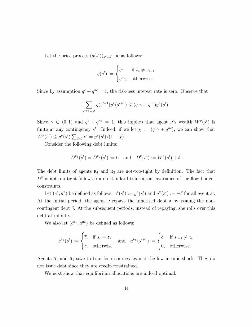
Let the price process (q(st))st�s0 be as follows:
q(st) :=
qc, if st 6= st−1
qnc, otherwise.
Since by assumption qc + qnc = 1, the risk-less interest rate is zero. Observe that∑st+1�st
q(st+1)yp(st+1) ≤ (qcγ + qnc)yp(st).
Since γ ∈ (0, 1) and qc + qnc = 1, this implies that agent p’s wealth W p(st) is
finite at any contingency st. Indeed, if we let χ := (qcγ + qnc), we can show that
W p(st) ≤ yp(st)∑
t≥0 χt = yp(st)/(1− χ).
Consider the following debt limits:
Dr1(st) = Dr2(st) := 0 and Dp(st) := W p(st) + δ.
The debt limits of agents r1 and r2 are not-too-tight by definition. The fact that
Dp is not-too-tight follows from a standard translation invariance of the flow budget
constraints.
Let (cp, ap) be defined as follows: cp(st) := yp(st) and ap(st) := −δ for all event st.
At the initial period, the agent p repays the inherited debt δ by issuing the non-
contingent debt δ. At the subsequent periods, instead of repaying, she rolls over this
debt at infinite.
We also let (crk , ark) be defined as follows:
crk(st) :=
c, if st = zk
c, otherwiseand ark(st+1) :=
δ, if st+1 6= zk
0, otherwise.
Agents r1 and r2 save to transfer resources against the low income shock. They do
not issue debt since they are credit-constrained.
We next show that equilibrium allocations are indeed optimal.
44

Observe that (cp, ap) is optimal since it is budget feasible (with equality) and
satisfies the Euler equations together with the individual transversality condition:
limt→∞
∑st∈St
βtπ(st)u′(cp(st))[ap(st) +Dp(st)] = u′(cp(s0)) limt→∞
∑st∈St
p(st)W (st) = 0.
The plan (crk , ark) is also optimal since it is budget feasible (with equality), it
satisfies the Euler equations and the individual transversality condition.24
Finally, all markets clear by construction.
References
Abraham, A. and Carceles-Poveda, E. (2010). Endogenous trading constraints with
incomplete asset markets. Journal of Economic Theory, 145(3):974–1004.
Aguiar, M., Amador, M., et al. (2014). Sovereign debt. Handbook of International
Economics, 4:647–687.
Aguiar, M. and Gopinath, G. (2006). Defaultable debt, interest rates and the current
account. Journal of International Economics, 69(1):64–83.
Alvarez, F. and Jermann, U. J. (2000). Efficiency, equilibrium, and asset pricing with
risk of default. Econometrica, 68(4):775–797.
Alvarez, F. and Jermann, U. J. (2001). Quantitative asset pricing implications of
endogenous solvency constraints. Review of Financial Studies, 14(4):1117–1151.
Arellano, C. (2008). Default risk and income fluctuations in emerging economies.
American Economic Review, 98(3):690–712.
24The transversality condition is satisfied because the equilibrium is Markovian stationary. For-mally, we have ∑
st∈St
βtπ(st)u′(crk(st))ark(st) ≤ βtu′(c)δ −−−→t→∞
0.
45

Bai, Y. and Zhang, J. (2010). Solving the Feldstein–Horioka puzzle with financial
frictions. Econometrica, 78(2):603–632.
Bai, Y. and Zhang, J. (2012). Financial integration and international risk sharing.
Journal of International Economics, 86(1):17–32.
Bulow, J. and Rogoff, K. (1989). Sovereign debt: Is to forgive to forget? American
Economic Review, 79(1):43–50.
Caballero, R. J., Farhi, E., and Gourinchas, P.-O. (2008). An equilibrium model
of global imbalances and low interest rates. The American Economic Review,
98(1):358.
Cohen, D. and Sachs, J. (1986). Growth and external debt under risk of debt repu-
diation. European Economic Review, 30(3):529–560.
Cole, H. and Kehoe, T. J. (2000). Self-fulfilling debt crises. Review of Economic
Studies, 67(1):91–116.
Diamond, P. A. (1965). National debt in a neoclassical growth model. The American
Economic Review, 55(5):1126–1150.
Farhi, E. and Tirole, J. (2012). Bubbly liquidity. The Review of economic studies,
79(2):678–706.
Geanakoplos, J. and Zame, W. (2002). Collateral and the enforcement of intertem-
poral contracts. Discussion Paper, Yale University.
Gennaioli, N., Martin, A., and Rossi, S. (2014). Sovereign default, domestic banks,
and financial institutions. The Journal of Finance, 69(2):819–866.
Gottardi, P. and Kubler, F. (2015). Dynamic competitive equilibrium with complete
markets and collateral constraints. Review of Economic Studies, 82:1119–1153.
Hellwig, C. and Lorenzoni, G. (2009). Bubbles and self-enforcing debt. Econometrica,
77(4):1137–1164.
46

Hirano, T. and Yanagawa, N. (2016). Asset bubbles, endogenous growth, and financial
frictions. The Review of Economic Studies, 84(1):406–443.
Holmstrom, B. and Tirole, J. (1998). Private and public supply of liquidity. Journal
of political Economy, 106(1):1–40.
Holmstrom, B. and Tirole, J. (2011). Inside and outside liquidity. MIT press.
J. Caballero, R. and Farhi, E. (2017). The safety trap. The Review of Economic
Studies, page rdx013.
Kehoe, P. and Perri, F. (2004). Competitive equilibria with limited enforcement.
Journal of Economic Theory, 119(1):184–206.
Kehoe, T. J. and Levine, D. K. (1993). Debt-constrained asset markets. Review of
Economic Studies, 60(4):865–888.
Kletzer, K. and Wright, B. (2000). Sovereign debt as intertemporal barter. American
Economic Review, 90(3):621–639.
Kocherlakota, N. (1996). Implications of efficient risk-sharing without commitment.
Review of Economic Studies, 63(4):595–609.
Kubler, F. and Schmedders, K. (2003). Stationary equilibria in asset-pricing models
with incomplete markets and collateral. Econometrica, 71(6):1767–1795.
Martin, A. and Ventura, J. (2012). Economic growth with bubbles. The American
Economic Review, 102(6):3033–3058.
Martins-da-Rocha, V. F. and Vailakis, Y. (2016). On the sovereign debt paradox.
Economic Theory, electronic copy available at https://doi.org/10.1007/s00199-016-
0971-6.
Martins-da-Rocha, V. F. and Vailakis, Y. (2017). Borrowing in excess of natural
ability to repay. Review of Economic Dynamics, 23:42–59.
47

Mendoza, E. G. and Yue, V. Z. (2012). A general equilibrium model of sovereign
default and business cycles. The Quarterly Journal of Economics, 127(2):889–946.
Miao, J. and Wang, P. (2011). Bubbles and credit constraints. Mimeo.
Phan, T. (2017). Sovereign debt signals. Journal of International Economics, 104:157–
165.
Santos, M. and Woodford, M. (1997). Rational asset pricing bubbles. Econometrica,
65(1):19–57.
Tirole, J. (1985). Asset bubbles and overlapping generations. Econometrica: Journal
of the Econometric Society, pages 1071–1100.
Tomz, M. and Wright, M. L. J. (2013). Empirical research on sovereign debt and
default. Annual Review of Economics, 5:247–272.
Trebesch, C., Papaioannou, M. G., and Das, U. S. (2012). Sovereign debt restruc-
turings 1950-2010; literature survey, data, and stylized facts. Technical report,
International Monetary Fund.
Woodford, M. (1990). Public debt as private liquidity. The American Economic
Review, 80(2):382–388.
48