Self Control, Risk Aversion, and the Allais Paradox

Drew Fudenberg* and David K. Levine**

First Version: May 12, 2006

This Version: September 4, 2008

* Department of Economics, Harvard University

** Department of Economics, Washington University in St. Louis

We thank Daniel Benjamin and Jesse Shapiro for helpful comments and a verycareful reading of an early draft. We are also grateful to Juan Carillo, Ed Glaeser,Glenn Harrison, John Kagel, Drazen Prelec, and seminar participants at Ohio Stateand the 2006 CEPR conference on Behavioral Economics.

1

1. Introduction

Behavioral economics is replete with models designed to explain particular

anomalies ranging from intertemporal choice to risk and addiction. However, to do more

than simply organize the data from a given experiment, a model should fit behavior in a

reasonably broad class of settings; it is much better to have a small number of models that

explain a large number of facts than the reverse. Ideally, a model should not only predict

the data it was fit to, but also make correct predictions about outcomes in other settings,

including experiments that have not yet been run. As a step towards that goal, Fudenberg

and Levine [2006] studied a self-control problem derived from a game between a single

long-lived self and a sequence of short-term myopic selves. This “dual-self” model not

only yields a dynamic model of intertemporal choice consistent with those widely and

successfully used in macroeconomics, it predicts many behavioral anomalies seen in the

laboratory. In particular, while it is designed to be a time-consistent explanation of

hyperbolic discounting, the model predicts the Rabin paradox of inconsistent risk

aversion between small and large gambles. It also makes predictions about the impact of

cognitive load on decision making. Fudenberg and Levine [2006] argued that existing

data on cognitive load suggests that the cost of self-control is convex and not linear. If

that is true, then choices involving relatively less tempting options will be aligned with

the preferences of the long-run self, while choices involving more tempting options will

be aligned with the preferences of the short-run self. In this paper we argue this is

supported by evidence, and that one of the predictions that follows from a convex cost of

self-control is that there should be an Allais paradox.

Our goal in this paper is to show that a dual self model compatible with modern

dynamic macroeconomic models and using a single set of calibrated parameters is both

consistent with macroeconomic evidence and quantitatively predicts a wide range of

behavioral anomalies: the Rabin paradox, the Allais paradox, and the effect of cognitive

load on decisions involving risk.

To obtain a quantitative fit, as opposed to simply showing that the model allows

the anomalies, we extend the model of Fudenberg and Levine [2006] and introduce an

additional parameter. That paper showed how the equilibrium of a game between a single

long-lived patient self and a sequence of short-term myopic selves is equivalent to

optimization by a single long-run agent with a “cost of self-control.” It then specialized

2

the model to the case where the cost of self-control depends only on the short-run utility

of the chosen action and the short-run utility of the most tempting alternative. We argued

that a number of experimental and empirical observations suggest that the cost function is

convex, and that this convexity in turn implies that the reduced form of the dual-self

model fails the independence axiom of expected utility theory.1

The convexity of the cost function leads to a particular sort of violation of the

independence axiom: Agents should be “more rational” about choices that are likely to be

payoff-irrelevant. This is exactly the nature of the violation of the independence axiom

in the Allais paradox. In the Allais paradox there are two scenarios each involving two

options. Under expected utility theory, the same option must be chosen in each scenario,

but in practice people choose different options in the two scenarios. A key element of the

paradox is that one of the scenarios involves a much smaller probability of winning a

prize. That means that there is less temptation to the short-run self. With convex cost of

self-control, less temptation means lower marginal cost of self-control, and consequently

that it is optimal for the long-run self to exert more self control and so choose the lottery

with the highest long-run utility. Because the long-run self is patient and the lottery is a

small share of lifetime wealth, this will be the lottery with the higher expected value.

When the chance of winning a prize is high, the temptation great, so the marginal cost of

self-control high. In this case, so the long-run self should allow the short-run self to

choose the lottery. Since short-run utility will be essentially the same regardless of

whether the prize is large or small, the short-run self prefers the lottery with the highest

probability of winning a prize. This is exactly the sort of reversal observed in the Allais

paradox. We should emphasize that our theory does not explain all possible violations of

1 The work of Baumeister and collaborators (for example, Muraven et al [1998,2000], Galiot et al [2008])argues that self-control is a limited resource, moreover one that may be measured by blood glucose levels.The stylized fact that people often reward themselves in one domain (for example, food) when exertingmore self control in another (for example, work) has the same implication. This is backed up by evidencefrom Shiv and Fedorikhin [1999] and Ward and Mann [2000] showing that agents under cognitive loadexercise less self-control, for example, by eating more deserts. The first two observations fit naturally withthe idea that a common “self-control function” controls many nearly simultaneous choices. The third fitsnaturally with the hypothesis that self-control and some other forms of mental activity draw on relatedmental systems or resources. Benahib and Bisin [2005], Bernheim and Rangel [2004], Brocas and Carillo[2005], Loewenstein and O’Donoghue [2005] and Ozdenoren et al [2006] present similar dual-self models,but they do not derive them from a game the way we do, and they do not discuss risk aversion, cognitiveload, or the possibility of convex costs of self-control.

3

the independence axiom: If the choices in each of the two Allais scenarios were reversed,

the independence axiom would still be violated, but our explanation would not apply.

Our goals in this paper are not only to formalize the analysis of the Allais

paradox, but to construct a form of the dual-self model that can be calibrated to explain a

range of data about choices over lotteries. To do this, we extend the bank/nightclub

model we used in Fudenberg and Levine [2006] by adding an additional choice of

“consumption technology.” This is necessary not only to explain the Allais paradox, but

to explain substantial risk aversion even to the very small stakes used in some

experiments. Specifically, while our earlier model can explain the examples in Rabin

[2000], those examples (such as rejecting a bet that had equal probability of winning

$105 or losing $100) understate the degree of risk aversion in small-stakes experiments

where agents are risk averse over much smaller gambles.

The idea of the bank/nightclub model is that agents use cash on hand as a

commitment device, so that on the margin they will consume all of any small unexpected

winnings. However, when agents win large amounts, they choose to exercise self-control

and save some of their winnings. The resulting intertemporal smoothing make the agents

less risk averse, so that they are less risk averse to large gambles than to small ones.

When calibrating the model to aggregate data, we took the underlying utility function to

be logarithmic and the same for all consumers. In the present paper we show that this

simple specification is not consistent with experimental data on risk aversion and

reasonable values of the pocket cash variable against which short-term risk is compared.2

For this reason we introduce an extension of the nightclub model in which the choice of

venue at which short-term expenditures are made is endogenous. This reflects the idea

that over a short period of time, the set of things on which the short-run self can spend

money is limited, so the marginal utility of consumption decreases fairly rapidly and risk

aversion is quite pronounced. Over a longer time frame there are more possible ways to

adjust consumption, and also to learn how to use or enjoy goods that have not been

consumed before, so that the long-run utility possibilities are the upper envelope of the

2 Since the first version of this paper was written, Cox et al [2007] conducted a series of experiments to testvarious utility theories using relatively high stakes. They also observe that the simple logarithmic model isinconsistent with observed risk aversion, and they argue that the simple linear-logarithmic self-controlmodel does not plausibly explain their data. We will be interested to see whether their data is consistentwith the more complex model developed here.

4

family of short-run utilities. With the preference that we specify in this paper, this upper

envelope, and thus the agent’s preferences over steady state consumption levels, reduces

to the logarithmic form we used in our previous paper.

After developing the theory of “endogenous nightclubs,” we then calibrate it in an

effort to examine three different paradoxes. Specifically, we analyze Rabin paradox data

from Holt and Laury [2002], the Kahneman and Tversky [1979] and Allais versions of

the Allais paradox, and the experimental results of Benjamin, Brown, and Shapiro

[2006], who find that exposing subjects to cognitive load increases their small-stakes risk

aversion.3

Our procedure is to find a set of sensible values of the key parameters, namely

the subjective interest rate, income, the degree of short-term risk aversion, the time-

horizon of the short-run self, and the degree of self-control, using a variety of external

sources of data. We than ask investigate how well we can explain the paradoxes using the

calibrated parameter values and the dual-self model. How broad of set of parameter

values in the calibrated range will explain the paradoxes? To what extent can the same set

of parameter values simultaneously explain all the paradoxes? Roughly speaking, we can

explain all the data if we assume an annual interest rate of 5%, a low degree of risk

aversion, and a daily time horizon for the short-run self. In the case of the Allais paradox,

we can find a degree of self-control for every interest rate/income/risk aversion

combination in the calibrated range that explains the paradox. We find that the Rabin

paradox is relatively insensitive to the exact parameters assumed; the Allais paradox is

sensitive to choosing a plausible level of risk aversion; and the Chilean cognitive load

data is very sensitive to the exact parameter values chosen.

After showing that the base model provides a plausible description of data on

attitudes towards risk, gambles, and cognitive load, we examine the robustness of the

3 The main focus of Benjamin, Brown and Shapiro [2006], like that of Frederick [2005], is on thecorrelation between measures of cognitive ability and the phenomena of small-stakes risk aversion and of apreference for immediate rewards. Benjamin, Brown and Shapiro find a significant and substantialcorrelation between with each of these sorts of preferences and cognitive ability. They also note that thecorrelation between cognitive ability and time preference vanishes when neither choice results in animmediate payoffs, and that the correlation between small-stakes risk aversion and “present bias” drops tozero once they control for cognitive ability. This evidence is consistent with our explanation of the Rabinparadox, as it suggests that that small-stakes risk aversion results from the same self-control problem thatleads to a present bias in the timing of rewards. They also discuss the sizable literature that examines thecorrelation between cognitive ability and present bias without discussing risk aversion.

5

theory. Specifically, in the calibrations we assume that the opportunities presented in the

experiments are unanticipated, so we consider what happens when gambling

opportunities are foreseen.

2. Self-Control, Cash Constraints, and Target Consumption

Fudenberg and Levine [2006] considered a “self control game” between a single

long run patient self and a sequence of short-run impulsive selves each of whom lives for

a single period. The equilibria of this game correspond to the solutions to a “reduced

form maximization” of a single long-run self whose objective is the expected present

value of the utility of the short-run selves net of a cost of self-control. To develop this

model, we start by detailing the decision problem and the utility of the short-run selves.

At the end of this section we will relate these short-run utility functions to the reduced

form maximization of the long-run self.

We consider an infinite-lived consumer making a savings decision. Each period

����T � ! is divided into two sub-periods, the bank subperiod and the nightclub

subperiod. Wealth at the beginning of the bank sub-period is denoted by TW . During the

“bank” subperiod, consumption is not possible, and wealth is divided between savings TS ,

which remains in the bank, pocket cash TX which is carried to the nightclub, and durable

consumption DTC which is paid for immediately and is consumed in the second sub-period

of period T .4 In the nightclub consumption �T TC Xb b is determined, with

T TX C�

returned to the bank at the end of the period. Wealth next period is just

� � DT T T T TW 2 S X C C� � � � � . For simplicity money returned to the bank bears the same

rate of interest as money left in the bank. No borrowing is possible, and there is no other

source of income other than the return on investment.

Consumption Commitment: So far, we have followed Fudenberg and Levine [2006].

Now we consider an extension of their model that we will need to explain the degree of

risk aversion we observe in experimental data. Specifically, we suppose that there is a

4 Durable and/or committed consumption is a significant fraction (roughly 50%) of total consumption so weneed to account for it in calibrating the model, but consumption commitments are not our focus here. Forthis reason we use a highly stylized model, with consumption commitments reset at the start of each timeperiod. A more realistic model of durable consumption would have commitments that extend for multiplepeiods, as in Grossman and Laroque [1990].

6

choice of nightclubs to go to in the nightclub sub-period. These choices are indexed by

the quality of the nightclub ��� TC � d . In a nightclub of quality TC we assume that

the utility of the short-run self has the form � \ T TU C C depending on the amount

consumed TC there and the quality of the nightclub.

The utility function at the nightclub is assumed to satisfy � \ � \ T T T TU C C U C Cb .

This means that when planning to consume a given amount TC it is best to choose the

nightclub of the same index. Intuitively, the quality TC of a nightclub represents a

“target” level of consumption expenditure at that nightclub. That is, if you are going to

consume a low level of TC you would prefer to spend it at a nightclub with a low value of

TC and you would like to consume a high level of TC at a high quality nightclub.

It is useful to think of a low value of TC as representing a nightclub that serves

cheap beer, while a high value of TC represents a nightclub that serves expensive wine.

At the beer bar TC represents expenditure on cheap beer, while at the wine bar it

represents the expenditure on expensive wine. The assumption that� \ � \ T T T TU C C U C Cb captures the idea that spending a large amount at a low quality

nightclub results in less utility than spending the same amount at a high quality nightclub:

lots of cheap beer is not a good substitute for a nice bottle of wine. Conversely, spending

a small amount at a high quality night club results in less utility than spending the same

amount at a low quality nightclub: a couple of bottles of cheap beer are better than a

thimble-full of nice wine. People with different income and so different planned

consumption levels will choose consumption sites with different characteristics. The

quality of a nightclub can also be interpreted as a state variable or capital stock that

reflects experience with a given level of consumption: a wine lover who unexpectedly

wins a large windfall may take a while to both to learn to appreciate differences in grands

crus and to learn which ones are the best values.5

We assume that the base preference of the short-run self satisfies

� \ LOGT T TU C C C� ; this ensures that in a deterministic and perfectly foreseen environment

without self control costs, behavior is the same as with standard logarithmic preferences.

To avoid uninteresting approximation issues, we assume that there are a continuum of

5 To fully match the model, this state variable needs to reflect only recent experience: a formerly wealthywine lover who has been drinking vin de table for many years may take a while to reacquire both adiscerning palate and up-to-date knowledge of the wine market.

7

different kinds of nightclubs available, so that there are many intermediate choices

between the beer bar and wine bar.

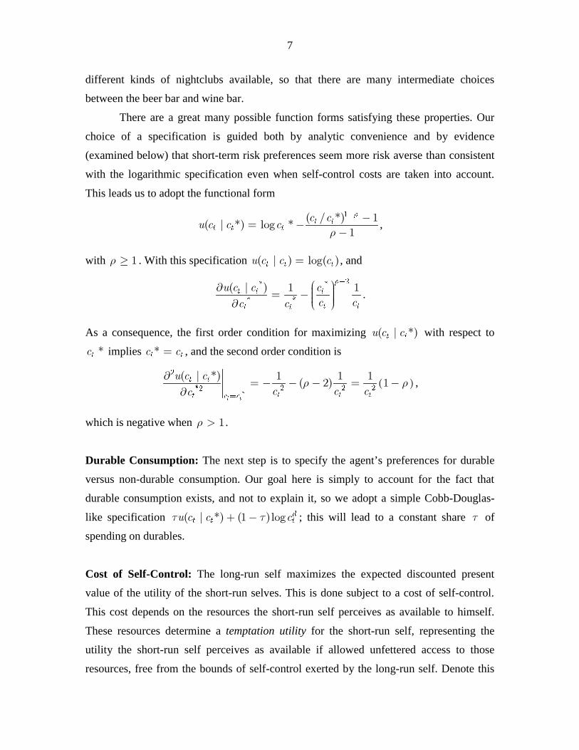
There are a great many possible function forms satisfying these properties. Our

choice of a specification is guided both by analytic convenience and by evidence

(examined below) that short-term risk preferences seem more risk averse than consistent

with the logarithmic specification even when self-control costs are taken into account.

This leads us to adopt the functional form

�� � �� \ LOG

�T T

T T T

C CU C C C

S

S

� �� �

�,

with �S p . With this specification � \ LOG� T T TU C C C� , and

�

� \ � �T T T

T TT T

U C C CC CC C

S�� ¬s ­�� � ­� ­­�s � ®.

As a consequence, the first order condition for maximizing � \ T TU C C with respect to

TC implies T TC C� , and the second order condition is

�

� � ��

� \ � � �� �

T T

T T

T T TT C C

U C CC C CC

S S�

s� � � � � �

s,

which is negative when �S � .

Durable Consumption: The next step is to specify the agent’s preferences for durable

versus non-durable consumption. Our goal here is simply to account for the fact that

durable consumption exists, and not to explain it, so we adopt a simple Cobb-Douglas-

like specification � \ �� LOG DT T TU C C CU U� � ; this will lead to a constant share U of

spending on durables.

Cost of Self-Control: The long-run self maximizes the expected discounted present

value of the utility of the short-run selves. This is done subject to a cost of self-control.

This cost depends on the resources the short-run self perceives as available to himself.

These resources determine a temptation utility for the short-run self, representing the

utility the short-run self perceives as available if allowed unfettered access to those

resources, free from the bounds of self-control exerted by the long-run self. Denote this

8

temptation utility by TU . The actual realized utility that the long-run self allows the short-

run self is TU , and there may be cognitive load due to other activities, TD . Then the cost of

self-control is � T T TG D U U� � and where the function g is continuously differentiable

and convex. Until section 7 we suppose that there is no cognitive load from other

activities, and set �TD � . The key idea here is that the cost of self-control depends on the

difference between the utility the short-run self is tempted by TU and the utility the short-

run self is allowed TU . In our calibrations of the model, we will take the cost function to

be quadratic: �� ����T T TG V V VH� � ( .

Long-run Self: In the bank no consumption is possible, and so there is no temptation for

the short-run self. In the nightclub the short-run self cannot borrow, and wishes to spend

all of the available pocket cash tx on consumption. This pocket cash functions as a

commitment device: by spending money on durable consumption or leaving it in the

bank, it is not available to the short-run self in the nightclub, so does not represent a

temptation that must be overcome by costly self-control.

The problem faced by the long-run self is to choose pocket cash and consumption

to maximize the present value using the discount factor E of short-run self utility net of

the cost of self-control. The objective function of the long-run self is

�

�� \ � � \ � \ �� LOG

2&

T DT T T T T T T

T

5

% U C C G U X C U C C CE U Ud�

�

�

  ¯� � � �¢ ±� (2.1)

which is to be maximized with respect to �� �� �� �DT T T TC C C Xp p p p subject to �W

given, � � DT T T T TW 2 S X C C� � � � � , T T TS X W� b and �TW p .

In this formulation there is a single long-run self with time-consistent preferences.

Although the impulsive short-run selves are the source of self-control costs, the

equilibrium of the game between the long run self and the sequence of short run selves is

equivalent to the optimization of this reduced-form control problem by the single long-

run self.

Solution in the Deterministic Case: Suppose that there is no uncertainty, so this is a

simple deterministic infinite-horizon maximization problem. Because there is no cost of

self-control in the bank, the solution to this problem is to choose

T T TC C X� � . In other

9

words, cash TX is chosen to equal the optimal consumption for an agent without self-

control costs, and

TC is the nightclub of the same quality. The agent then spends all

pocket cash at the nightclub, and so incurs no self-control cost there. Since

T T TC C X� � ,

the utility of the short run self is � \ LOGT T TU X C X� , and as there is no self-control cost,

this boils down to maximizing

�

�LOG �� LOG T D

T TT

X CE U Ud�

�

  ¯� �¢ ±�

subject to the budget constraint � � DT T T TW 2 W X C� � � � . The solution is easily

computed6 to be �� T TX WE U� � , and �� �� DT TC WU E� � � . The corresponding

present value utility of the long-run self is

�

� �

LOG� �

�W

5 W +E

� ��

,

where

< >�

LOG�� LOG� LOG �� LOG�� �

+ 2E E E U U U UE

� � � � � � ��

.

These together give the solution of the simple deterministic budget problem.

Implications of Uncertainty: The deterministic savings model is too simple to account

for any behavioral phenomena. However, the situation changes when there is

uncertainty. Suppose that unexpectedly the short-run self at the nightclub is offered a

choice between a dollar today and two dollars tomorrow. Despite the preference (for any

reasonable discount factor) of the long-run self for the dollar tomorrow, and the fact that

given the choice between tomorrow and the day after the long-run self will commit to the

day after, the long-run self may well allow the short-run self to take the dollar today. The

reason is simply that the short-run self was rationed by TX . The extra dollar today

represents a temptation that is costly for the long-run self to control. If that cost of self-

control exceed the benefit of an extra dollar tomorrow, the short-run self will be allowed

to take the extra dollar today.

6 The derivation is standard; an explicit computation in the case where �U � is in Fudenberg and Levine[2007]. Note that equation (1) of that paper contains a typographical error: in place of

��� LOG�� LOGA YH� � � it should read ��� LOG�� LOG� A YH� � � .

10

The demand for costly self-commitment in order to reduce the future cost of self-

control has many implications. For example, individuals may pay a premium to invest in

illiquid assets, as do the quasi-hyperbolic agents in Laibson [1997]. They may also

choose to carry less cash than in the absence of self-control costs, as they do here.

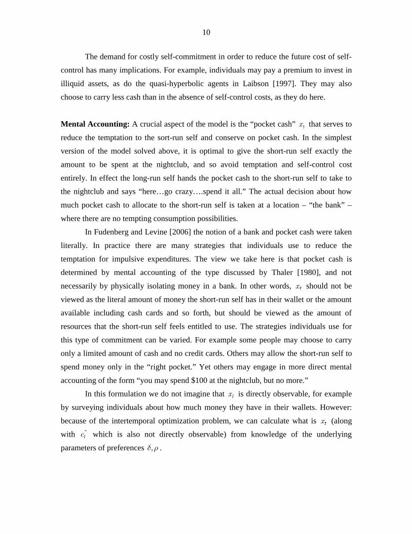
Mental Accounting: A crucial aspect of the model is the “pocket cash” TX that serves to

reduce the temptation to the sort-run self and conserve on pocket cash. In the simplest

version of the model solved above, it is optimal to give the short-run self exactly the

amount to be spent at the nightclub, and so avoid temptation and self-control cost

entirely. In effect the long-run self hands the pocket cash to the short-run self to take to

the nightclub and says “here…go crazy….spend it all.” The actual decision about how

much pocket cash to allocate to the short-run self is taken at a location – “the bank” –

where there are no tempting consumption possibilities.

In Fudenberg and Levine [2006] the notion of a bank and pocket cash were taken

literally. In practice there are many strategies that individuals use to reduce the

temptation for impulsive expenditures. The view we take here is that pocket cash is

determined by mental accounting of the type discussed by Thaler [1980], and not

necessarily by physically isolating money in a bank. In other words, TX should not be

viewed as the literal amount of money the short-run self has in their wallet or the amount

available including cash cards and so forth, but should be viewed as the amount of

resources that the short-run self feels entitled to use. The strategies individuals use for

this type of commitment can be varied. For example some people may choose to carry

only a limited amount of cash and no credit cards. Others may allow the short-run self to

spend money only in the “right pocket.” Yet others may engage in more direct mental

accounting of the form “you may spend $100 at the nightclub, but no more.”

In this formulation we do not imagine that TX is directly observable, for example

by surveying individuals about how much money they have in their wallets. However:

because of the intertemporal optimization problem, we can calculate what is TX (along

with

TC which is also not directly observable) from knowledge of the underlying

parameters of preferences �E S .

11

3. Risky Drinking: Nightclubs and Lotteries

Suppose in period 1 (only) that when the agent arrives at the nightclub of her

choice, she has the choice between two lotteries, A and B with returns � ��! "Z Z� � . Initially

we will assume that this choice is completely unanticipated – that is, it has prior

probability zero. This means that �� T T TC X WE U� � � . What is the optimal choice of

lottery given �X C ? For simplicity – and without much loss of generality7 – we assume

throughout that following the end of period 1 no further lottery opportunities at night

clubs are anticipated.

The lotteries �Z Z� � may involve gains or losses, but we suppose that the largest

possible loss is less than the agent’s pocket cash. There are number of different ways that

the dual-self model can be applied to this setting, depending on the timing and

“temptingness” of the choice of lottery and spending of its proceeds. In this section, we

restrict attention to case in which the short-run self in the nightclub simultaneously

decides which lottery to pick and how to spend for each possible realization of the lottery.

Since the highest possible short-run utility comes from consuming the entire

proceed of the lottery, the temptation utility is

� � � � � �MAX[ � � � � � ]! "%U X Z C %U X Z C� �� �

where �

JZ� is the realization of lottery �J ! "� . This temptation must be compared to the

expected short-run utility from the chosen lottery. If we let � �� J JC Z� be the consumption

chosen contingent on the realization of lottery j, the self-control cost is

� � � � � � ��MAX[ � � � � � ] � � J! "G %U X Z C %U X Z C %U C C� � �� � � .

Let �H denote the marginal cost of self-control in the first period. We let �� �e � � J JC ZH be

the solution to the first-order condition for a maximum for a given marginal cost of self

control, that is, the unique solution to

��

� � �� � �

�� �� � J J J DC C W Z C C

SS U E H

E� � �

� � � � ,

and find the corresponding marginal cost of self control

7 The overall savings and utility decision will not change significantly provided that the probability ofgetting lottery opportunities – whether anticipated or not – at the nightclub are small.

12

�

� � � � � � � �� � �

e �

e��MAX[ � � � � � ] �MIN[ � � � ]�

J

J J J! "G %U X Z C %U X Z C %U C Z X Z C

H H

H

�

� � � �� � � �

We show in the Appendix that we can characterize the optimum as follows:

Theorem 1: For given

� �� � X C and each [ � ]J ! "� there is a unique solution to

� � �e � J J JH H H�

and this solution together with � �� � � �eMIN� � � � ]J J J J*C C Z X ZH� �� and the choice of J that

maximizes long-run utility is necessary and sufficient for an optimal solution to the

consumer’s choice between lotteries A and B.

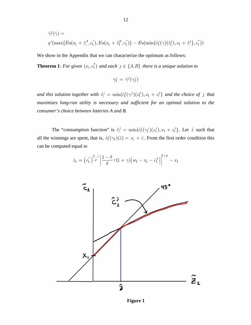
The “consumption function” is �� � � � �eMIN� � � � ]J J J J JC C Z X ZH� �� . Let eZ such that

all the winnings are spent, that is, � ��e e e� � JC Z X ZH � � . From the first order condition this

can be computed equal to

� ��

� � � � � �

�e �� DZ C W X C X

S S

SE U H

E

� �  ¯  ¯� � � � �¡ °¢ ±¢ ±

Figure 1

13

Note that for arbitrary

� ��X C we may have �eZ negative. This is sketched in Diagram 1.

For ��eJZ Z� no self-control is used, and all winnings are spent. Above this level self

control is used, with only a fraction of winnings consumed, and the rest going to savings.

When the time period is short, �eJC is very flat, so that only a tiny fraction of the winnings

are consumed immediately when receipts exceed the critical level. Thus when the agent is

patient he is almost risk neutral with respect to large gambles. However the agent is still

risk averse to small gambles, as these will not be smoothed but will lead to a one for one

change in current consumption.

4. Basic Calibration

The first step in our calibration of the model is to pin down as many parameters as

possible using estimates from external sources of data. We will subsequently use data

from laboratory experiments to calibrate risk aversion parameters and to determine the

cost of self control.

To measure the subjective interest rate R we ordinarily think of taking the

difference between the real rate of return and the growth rate of per capital consumption.

However, we must contend with the equity premium puzzle. From Shiller [1989], we see

that over a more than 100 year period the average growth rate of per capita consumption

has been 1.8%, the average real rate of returns on bonds 1.9%, and the real rate of return

on equity 7.5%. Fortunately if the consumption lock-in once a nightclub is chosen lasts

for six quarters,8 the problem of allocating a portfolio between stocks and bonds is

essentially the same as that studied by Gabaix and Laibson [2001], which is a simplified

version of Grossman and Laroque [1990].9 Their calibrations support an interest rate of

1%, which we take as our primary case. For robustness, we also use 3% and 5%, the

latter being at the high range of what can be supported by Shiller’s data.

From the Department of Commerce Bureau of Economic Analysis, real per capita

disposable personal income in December 2005 was $27,640. To consider a range of

8 We have implicitly assumed it lasts for only a day, but the length of lock-in plays no role in the analysis,no result or calculation changes if the lock-in is six quarters.9 They assume that once the nightclub is chosen, no other level of consumption is possible. We allowdeviations from the nightclub level of consumption – but with very sharp curvature, so in practiceconsumers are “nearly locked in” to their choice of nightclub. Chetty and Szeidl [2006] show that thesemodels of sticky consumption lead to the same observational results as the habit formation models used byConstantinides [1990] and Boldrin, Christiano and Fisher [2001].

14

income classes, we will use three levels of income $14,000, $28,000, and $56,000. To

infer consumption from the data we do not use current savings rates, as these are badly

mis-measured due to the exclusion of capital gains from the national income accounts.

We instead use the historical long-term savings rate of 8% (see FSRB [2002]) measured

when capital gains were not so important. This enables us to determine wealth and

consumption from income.

We estimate wealth as annual consumption divided by our estimate of the

subjective interest rate R : � ����� �W Y R� , where �Y denotes steady state income. In

determining pocket cash, we need take account of consumption DTC that is not subject to

temptation: housing, consumer durables, and medical expenses. At the nightclub, the rent

or mortgage was already paid for at the bank, and it is not generally feasible to sell one’s

car or refrigerator to pay for one’s impulsive consumption. As noted by Grossman and

Laroque [1990], such consumption commitments increase risk aversion for cash

gambles.10 Turning to the data, we use the National Income and Product Accounts from

the fourth quarter of 2005. In billions of current dollars, personal consumption

expenditure was $8,927.8. Of this $1,019.6 was spent on durables, $1,326.6 on housing,

and $1,534.0 on medical care, which are the non-tempting categories. This means that the

share of income subject to temptation ����U � .

Finally, we must determine the time horizon ∆ of the short-run self. This is hard

to pin down accurately, in part because it seems to vary both within and across subjects,

but the most plausible period seems to be about a day. For the purposes of robustness we

checked that none of our results are sensitive to assuming a time horizon of a week:

details can be found in the earlier working paper version available on line.

Putting together all these cases, we estimate pocket cash to be

� � ����� ���� ���� ������X Y Y� q q � q .

10 Chetty and Szeidl [2006] extend Grossman and Laroque to allow for varying sizes of gambles and costlyrevision of the commitment consumption. Postelwaite, Samuelson and Silberman [2006] investigate theimplications of consumption commitments for optimal incentive contracts.

15

Table 1

Percent interest r �Y � 14K �Y � 28K �Y � 56K

annual daily �W �X �W �X �W �X

1 .003 1.3M 2.6M 5.2M

3 .008 .43M .86M 1.7M

5 .014 .30M

20

.61M

40

1.2M

80

To determine a reasonable range of self control costs, we need to find how the

marginal propensity to consume “tempting” goods changes with unanticipated income.

The easiest way to parameterize this is with the “self-control threshold,” which is the

level of consumption at which self-control kicks in. The consumption cutoff

corresponding to �eZ is given by

< >

���

� � � � �

���

�� e e ��

�

C X Z X W

X

SS

S

S

U EH

E

H

� �  ¯w � � �¡ °

¡ °¢ ±x �

where we use the facts that � � � � �� W W X U Ex � � , and that �E x . Define

��� � � � �e� � �C XSN H H� � x . Because �H is measured in units of utility, its numerical

value is hard to interpret. For this reason we will report � �� N H rather than �H .

We can also relate �N to consumption data. Abdel-Ghany et al [1983] examined

the marginal propensity to consume semi- and non-durables out of windfalls in 1972-3

CES data.11 In the CES, the relevant category is defined as “inheritances and occasional

large gifts of money from persons outside the family...and net receipts from the

settlement of fire and accident policies,” which they argue are unanticipated. For

windfalls that are less than 10% of total income, they find a marginal propensity to

consume out of income of 0.94. For windfalls that are more than 10% of total income

they find a marginal propensity to consume out of income of 0.02. Since the reason for

11 The Imbens, Rubin and Sacerdote [2001] study of consumption response to unanticipated lotterywinnings shows that big winners earn less after they win, which is useful for evaluating the impact ofwinnings on labor supply. Their data is hard to use for assessing �N , because lottery winnings are paid as

an annuity and are not lump sum, so that winning reduces the need to hold other financial assets. It alsoappears as though the lottery winners are drawn from a different pool than the non-winners since winnersearn a lot less than non-winners before the lottery.

16

the 10% cutoff is not clear from the paper, we will view 10% as a general indication of

the cutoff. 12 As we have figured the ratio of income to pocket cash to be � �� ���Y X � ,

the value of �N corresponding to 10% of annual income is 69.6.

5. Small Stakes Risk Aversion

To demonstrate how the model works and calibrate the basic underlying model of

risk preference, we start with the “Rabin Paradox”: the small-stakes risk aversion

observed in experiments implies implausibly large risk aversion for large gambles.13 The

central issue is the case of small gambles. Following Rabin’s proposal, let option A be

��� � ������ � ���� , while option B is to get nothing. We expect that as Rabin predicts

many people will choose B. Since the combination of pocket cash and the maximum

winning is well below our estimates of �eC , all income is spent, and the consumer simply

behaves as a risk-averse individual with wealth equal to pocket cash and a coefficient of

relative risk aversion of S . Let us treat pocket cash as an unknown for the moment, and

ask how large could pocket cash be given that a logarithmic consumer is willing to reject

such a gamble. That is, we solve � � ��� LOG� ��� ��� ��� LN� X X X� � � � for pocket

cash; for larger values of 1x the consumer will accept the gamble, and for smaller ones he

will reject. In this sense, as Fudenberg and Levine [2006] argue, short-run logarithmic

preferences are consistent with the Rabin paradox.14

The problem with this analysis is that the gamble ��� � ������ � ���� has

comparatively large stakes. Laboratory evidence shows that subjects will reject

considerably smaller gambles, which is harder to explain with short-run logarithmic

preferences. We use data from Holt and Laury [2002], who did a careful laboratory study

of risk aversion. Their subjects were given a list of ten choices between an A and a B

lottery. The specific lotteries are shown below, where the first four columns show the

12 Landsburger [1966] with both CES data and with data on reparation payments by Germany to Israelicitizens reaches much the same conclusion.13 Rabin thus expands on an earlier observation of Samuelson [1963].14 Note that this theory predicts that if payoffs are delayed sufficiently, risk aversion will be much lower.Experiments reported in Barberis, Huang and Thaler [2003] suggest that there is appreciable risk aversionfor gambles where the resolution of the uncertainty is delayed as well as the payoffs themselves. However,delayed gambles are subject to exactly the same self-control problem as regular ones, so this is consistentwith our theory. In fact the number of subjects accepting the risky choice in the delayed gamble was in factconsiderably higher than the non-delayed gamble, rising from 10% to 22%.

17

probabilities of the rewards, and the first four rows, which are irrelevant to our analysis

are omitted.

Table 2

Option A Option B Fraction of Subjects Choosing A

$2.00 $1.60 $3.85 $0.10 1X 20X 50X 90X

0.5 0.5 0.5 0.5 .70 .85 1.0 .90

0.6 0.4 0.6 0.4 .45 .65 .85 .85

0.7 0.3 0.7 0.3 .20 .40 .60 .65

0.8 0.2 0.8 0.2 .05 .20 .25 .45

0.9 0.1 0.9 0.1 .02 .05 .15 .40

1.0 0.0 1.0 0.0 .00 .00 .00 .00

Initially subjects were told that one of the ten rows would be picked at random and they

would be paid the amount shown. Then they were given the option of renouncing their

payment and participating in a high stakes lottery, for either 20X, 50X or 90X of the

original stakes, depending on the treatment. The high-stakes lottery was otherwise the

same as the original: a choice was made for each of the ten rows, and one picked at

random for the actual payment. Everyone in fact renounced their winnings from the first

round to participate in the second. The choices made by subjects are shown in the table

above.

In the table we have highlighted (in yellow and turquoise respectively) the

decision problems where roughly half and 85% of the subjects chose A. We will take

these as characterizing median and high risk aversion respectively. The bottom 15th

percentile exhibits little risk aversion, suggesting that perhaps they do not face much in

the way of a self-control problem.

Since the stakes plus pocket cash remain well below our estimate of eC , we can fit

a CES with respect to our pocket cash estimates of $21, $42, $84, $155, $310 and $620,

in each case estimating the value of S that would leave a consumer indifferent to the

given gamble, assuming the chosen nightclub is equal to pocket cash. Taking the CES

functional form measured in units of marginal utility of income, we have for utility

18

�

� �

�

� � ��

C XX

S

S

� ��

�.

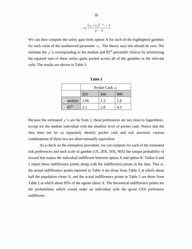
We can then compute the utility gain from option A for each of the highlighted gambles

for each value of the unobserved parameter �X . The theory says this should be zero. We

estimate the S ’s corresponding to the median and 85th percentile choices by minimizing

the squared sum of these utility gains pooled across all of the gambles in the relevant

cells. The results are shown in Table 3.

Table 3

Pocket Cash 1x

$20 $40 $80

S median 1.06 1.3 1.8

S 85th 2.1 2.8 4.3

Because the estimated S ’s are far from 1, these preferences are not close to logarithmic,

except for the median individual with the smallest level of pocket cash. Notice that the

data does not let us separately identify pocket cash and risk aversion; various

combinations of these two are observationally equivalent.

As a check on the estimation procedure, we can compute for each of the estimated

risk preferences and each scale of gamble (1X, 20X, 50X, 90X) the unique probability of

reward that makes the individual indifferent between option A and option B. Tables 4 and

5 report these indifference points along with the indifference points in the data. That is,

the actual indifference points reported in Table 4 are those from Table 2 at which about

half the population chose A, and the actual indifference points in Table 5 are those from

Table 2 at which about 85% of the agents chose A. The theoretical indifference points are

the probabilities which would make an individual with the given CES preference

indifferent.

19

Table 4: Indifference Probabilities for Median Estimated Value of S

Pocket cash and corresponding

median estimated S

$20,1.06 $40,1.3 $80,1.8

Actual indifference point Theoretical indifference points

1X .60 .47 .46 .46

20X .70 .65 .62 .60

50X .70 .72 .71 .71

90X .80 .79 .79 .81

Table 5: Indifference Probabilities for 85th Percentile Estimated Value of S

Pocket cash and corresponding

median estimated S

Actual Indifference point Theoretical indifference points

$20, 2.1 $40, 2.8 $80, 4.3

1X .70 .50 .48 .47

20X .80 .81 .79 .78

50X .90 .90 .91 .94

If the CES model fit the data perfectly then in each row the theoretical probabilities

corresponding to different levels of pocket cash would be identical to the actual

probabilities. For the 20X and above treatments the fit is quite good. However, the 1X

treatments fit less well suggesting that for very small gambles risk aversion is even

greater than for the CES.15

15 It is possible that the size of the choices might have been confounded with the order in which the choiceswere given. Harrison, Johnson, McInnes and Rutstrom [2005] find that corrected for order the impact of thesize of the gamble is somewhat less than Holt and Laurie found, a point which Holt and Laurie [2005]concede is correct. The follow-on studies which focus on the order effects do not contain sufficient data forus to get the risk aversion estimates we need.

20

6. The Allais Paradox

We proceed next to examine the Allais paradox in the calibrated model. We

assume that the choice in this (thought) experiment is completely unanticipated. In this

case the solution is simple: there is no self-control problem at the bank, so the choices is

� �C X� and spend all the pocket cash in the nightclub of choice. Given this, the problem

is purely logarithmic, so the solution is to choose � ��� X WE� � .

In the Kahneman and Tversky [1979] version of the Allais Paradox the two

options in the first scenario are �! given by ���� � ����� � �������� � ���� , while �" is

2400 for certain. Many people choose option �" . In scenario two the pair of choices are

�! � ���� � ����� � �������� � ���� and �" � ���� � ����� � ���� .16 Here many people

choose �! . Expected utility theory requires the same option ! or " be chosen in both

scenarios.

To describe the procedure we will use for reporting calibrations concerning

choices between pairs of gambles, let us examine in some detail the choice � ��! " in the

base case where the annual interest rate ��R � , annual income is $28,000, wealth is

$860,000, so pocket cash and the chosen nightclub are

� � ��X C� � .

Recall the cost of self-control �� � �� ����G V V VH� � ( . Consider first linear cost

of self-control, so that �( � . In this case we have an expected utility model, so the

optimal choice is independent of the scenario, and we can solve for the numerically

16 These were thought experiments. We are unaware of data from real experiments where subjects are paidover $2000, though experiments with similar “real stakes” are sometimes conducted poor countries. Thereis experimental data on the Allais paradox with real, but much smaller, stakes, most notably Battalio, Kageland Jiranyakul [1990]. Even for these very small stakes, subjects did exhibit the Allais paradox, and eventhe reverse Allais paradox. The theory here cannot explain the Allais paradox over such small amounts, asto exhibit the paradox, the prizes must be in the region of the threshold � �� N H , while the prizes in these

experiments ranged from $0.12 to $18.00, far out of this range. However, indifference or near indifferencemay be a key factor in the reported results. In set 1 and set 2 the two lotteries have exactly the sameexpected value, and the difference between the large and small prize is at most $8.00, and there was onlyone chance in fifteen that the decision would actually be implemented. So it is easy to imagine that subjectsdid not invest too much time and effort into these decisions. By way of contrast Harrison [1994] found thatwith various small stakes the Allais paradox was sensitive to using real rather than hypothetical payoffs,and found in the real payoff case only 15% of the population exhibited the paradox. Although ColinCamerer pointed out the drop from 35% when payoffs were hypothetical was not statistically significant, afollow study by Burke, Carter, Gominiak and Ohl [1996] found a statistically significant drop from 36% to8%. Conlisk [1989] also finds little evidence of an Allais paradox when the stakes are small. He examinespayoffs on the order of $10, much less than our threshold values of � �� N H of roughly 1% of annual

income. These studies suggest that when played for small real stakes there is no Allais paradox, as ourtheory predicts.

21

unique value �H ( � �� ����N H � ) such that there is indifference between the two

gambles A and B.17 A numerical computation shows that � � � �� � � � " !%U C %U CH H�� � ,

so that when �H is chosen so that the long-run self is indifferent, the short-run self

prefers the sure outcome B. On the other hand, when there is no cost of self-control, it is

easy to compute that the long-run self prefers the risky outcome ! .

Next, suppose that �( � . Suppose we have solved the optimization problem as

described by Theorem 1. As before, let �U be the temptation utility. This is calculated by

letting the short-run self choose the preferred lottery " and spend the entire proceeds.

We two possible values of the marginal cost of self-control separately depending

on whether option ! or option " is chosen by the long-run self.

� � � �

� � � �

� �

� �

! ! !

" " "

U %U C

U %U C

H H H

H H H

� � ( �

� � ( �

�

�(6.1)

Suppose we start with H slightly smaller than � H and �( � . Then in both scenarios

the risky option is strictly preferred. If we increase ( slightly then high temptation

scenario 1 �H will rise more than in the low temptation scenario 2, creating the possibility

that we will get a reversal in the high temptation scenario without creating a reversal in

the low temptation scenario. This is exactly the Allais paradox.

To verify that this construction works, we computed � H for each of our cases,

then constructed valued of �H ( with H close to � H and solved (6.1) iteratively to find

in scenario 1 � �;�=� ;�=! "H H and in scenario 2 � �;�=� ;�=! "H H . We the present value gain to the

risky option A over the safe option B in the two scenarios and verified that in fact B is

preferred in scenario 1 and A is preferred in scenario 2. The parameters used are reported

in Table 6.

(6.2)

17 Notice that this value will be the same if we consider the second pair of choices: with linear self-controlcost, the independence axiom is satisfied, and A and B are ranked the same way in both cases. Subsequentlywhen we add some curvature the indifference will be broken, and, as we shall see, in opposite ways for thefirst and second pair of choices.

22

Table 6 ��R �

income � � X C� S � �� N H H ( � �� ;�=!N H � �� ;�="N H � �� ;�=!N H � �� ;�="N H

14000 20 1.06 19.4 21.6 0.473 19.60 19.59 19.39 19.38

14000 20 2.10 7.19 26.5 23.9 7.35 7.20 6.76 6.61

28000 40 1.30 9.57 15.35 1.61 9.76 9.73 9.41 9.39

28000 40 2.80 4.03 10.4 37.3 4.16 4.05 3.82 3.71

56000 80 1.80 4.79 13.6 1.45 4.90 4.89 4.78 4.77

56000 80 4.20 2.45 2.57 58.4 2.50 2.42 2.34 2.26

Notice that the examples are relatively arbitrary. As can be seen by the wide range

of �H ( pairs that generate paradoxes in the various cases, there is in fact for each case a

wide range of parameters that will generate paradoxes. The basic limitation is that if the

curvature ( is chosen sufficiently large, then it will be impossible to generate values of

� ��! "H H that are sufficiently close to � H to give paradoxes.

The basic comparative static is driven by how the marginal cost of self-control

must change to maintain indifference between the two gambles in the face of changes in

the marginal utilities of current and future consumption. Recall that the short-run self

prefers the safe gamble B, while, starting in period 2 the long-run self prefers the risky

gamble A. If the marginal utility of current consumption increases relative to future

consumption, this will break the tie in favor of the earlier period, that is, the short-run

self. However, if lowering the marginal cost of self-control effectively lowers the weight

on the short-run self’s preferences, and restores the tie. The short version: more weight on

the present implies the marginal cost of self-control must fall.

The first comparative static we consider is to change the interest rate. If we

increase R to 3% or 5% then this increases the weight on the present, so must lower the

marginal cost of self-control. However, in the calibration when we change R we also

change wealth correspondingly. Changing R from 1% to 5% raises the weight on the

23

present period by a little more than a factor of 5, but is lowers wealth by a factor of 5, and

since second period value is logarithmic, raises the marginal utility of second period

wealth by a factor of 5. The net effect is a very small increase in the weight on the

present, and when we did the calculation, the values of � �� N H change only in the third

significant digit.

By way of contrast, raising risk aversion holding everything else fixed makes the

gamble less attractive to the short-run self, increasing the temptation. This effectively

increases the weight on the first period, so must lead to a reduced marginal cost of self-

control, as happens in Table 8. Increasing income has a different effect: it has little effect

on the decision problem, since that is formulated in relative terms. That means that the

cutoff in dollars cannot change much, and so the cutoff relative to pocket cash, which has

increased, must go down.

The values of the self-control parameter � �� N H range from 2.44-19.4, which is

considerably smaller than the 69.6 figure Abdel-Ghany et al [1983] found in CES data

that we discussed above. However, the windfall income in the CES is considerably larger

than these Allais gambles, so poses a greater temptation, and with increasing marginal

cost of self-control should generate higher marginal self-control costs.

Notice that we are able to explain the Allais paradox with exactly the same risk

aversion parameters that we used to explain the Rabin paradox. The theory here give a

consistent explanation of both paradoxes, and it does so with a decision model that is

consistent with long-run savings behavior being logarithmic as in growth and

macroeconomic models.

Original Allais Paradox: The original Allais paradox involved substantially higher

stakes, so it would be difficult to implement other than as a thought experiment. In the

original paradox where option �! was ���� � ����� � ������������ � ��������� and �"

was 1,000,000 for certain, the paradoxical choice is �" . The second scenario was �! �

���� � ����� � ��������� and �" � ���� � ����� � ��������� with the paradoxical choice

being �! . In our base case of median income the results for the original Allais paradox

are reported in Table 7.

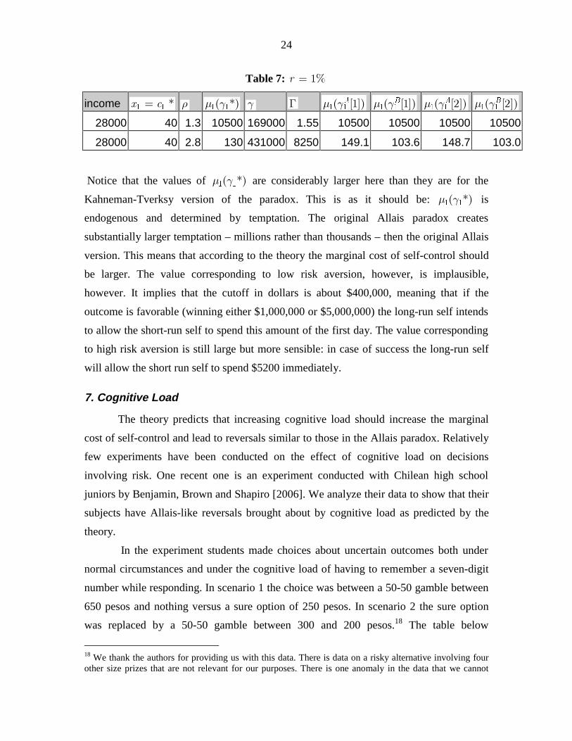
24

Table 7: ��R �

income � � X C� S � �� N H H ( � �� ;�=!N H � �� ;�="N H � �� ;�=!N H � �� ;�="N H

28000 40 1.3 10500 169000 1.55 10500 10500 10500 10500

28000 40 2.8 130 431000 8250 149.1 103.6 148.7 103.0

Notice that the values of � �� N H are considerably larger here than they are for the

Kahneman-Tverksy version of the paradox. This is as it should be: � �� N H is

endogenous and determined by temptation. The original Allais paradox creates

substantially larger temptation – millions rather than thousands – then the original Allais

version. This means that according to the theory the marginal cost of self-control should

be larger. The value corresponding to low risk aversion, however, is implausible,

however. It implies that the cutoff in dollars is about $400,000, meaning that if the

outcome is favorable (winning either $1,000,000 or $5,000,000) the long-run self intends

to allow the short-run self to spend this amount of the first day. The value corresponding

to high risk aversion is still large but more sensible: in case of success the long-run self

will allow the short run self to spend $5200 immediately.

7. Cognitive Load

The theory predicts that increasing cognitive load should increase the marginal

cost of self-control and lead to reversals similar to those in the Allais paradox. Relatively

few experiments have been conducted on the effect of cognitive load on decisions

involving risk. One recent one is an experiment conducted with Chilean high school

juniors by Benjamin, Brown and Shapiro [2006]. We analyze their data to show that their

subjects have Allais-like reversals brought about by cognitive load as predicted by the

theory.

In the experiment students made choices about uncertain outcomes both under

normal circumstances and under the cognitive load of having to remember a seven-digit

number while responding. In scenario 1 the choice was between a 50-50 gamble between

650 pesos and nothing versus a sure option of 250 pesos. In scenario 2 the sure option

was replaced by a 50-50 gamble between 300 and 200 pesos.18 The table below

18 We thank the authors for providing us with this data. There is data on a risky alternative involving fourother size prizes that are not relevant for our purposes. There is one anomaly in the data that we cannot

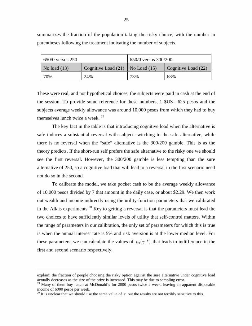
25

summarizes the fraction of the population taking the risky choice, with the number in

parentheses following the treatment indicating the number of subjects.

650/0 versus 250 650/0 versus 300/200

No load (13) Cognitive Load (21) No Load (15) Cognitive Load (22)

70% 24% 73% 68%

These were real, and not hypothetical choices, the subjects were paid in cash at the end of

the session. To provide some reference for these numbers, 1 $US= 625 pesos and the

subjects average weekly allowance was around 10,000 pesos from which they had to buy

themselves lunch twice a week. 19

The key fact in the table is that introducing cognitive load when the alternative is

safe induces a substantial reversal with subject switching to the safe alternative, while

there is no reversal when the “safe” alternative is the 300/200 gamble. This is as the

theory predicts. If the short-run self prefers the safe alternative to the risky one we should

see the first reversal. However, the 300/200 gamble is less tempting than the sure

alternative of 250, so a cognitive load that will lead to a reversal in the first scenario need

not do so in the second.

To calibrate the model, we take pocket cash to be the average weekly allowance

of 10,000 pesos divided by 7 that amount in the daily case, or about $2.29. We then work

out wealth and income indirectly using the utility-function parameters that we calibrated

in the Allais experiments.20 Key to getting a reversal is that the parameters must lead the

two choices to have sufficiently similar levels of utility that self-control matters. Within

the range of parameters in our calibration, the only set of parameters for which this is true

is when the annual interest rate is 5% and risk aversion is at the lower median level. For

these parameters, we can calculate the values of � �� N H that leads to indifference in the

first and second scenario respectively.

explain: the fraction of people choosing the risky option against the sure alternative under cognitive loadactually decreases as the size of the prize is increased. This may be due to sampling error.19 Many of them buy lunch at McDonald’s for 2000 pesos twice a week, leaving an apparent disposableincome of 6000 pesos per week.20 It is unclear that we should use the same value of U but the results are not terribly sensitive to this.

26

R income �W

� �X C� S � �� N H 1 � �� N H 2

5% 1.6K 29K 2.29 1.06 24.66 24.71

Note that the values of � �� N H of 24.66-24.71 needed to create indifference for the

Chilean gambles close to � �� ����N H � from the Allais paradox for the corresponding

5% calibration. As the temptations are of the same general order of magnitude, this

makes sense.

In both scenarios, the risky option has the greater temptation, meaning that it will

be chosen only for low marginal cost of self-control or equivalently, low values of � H .

The risky option, however, is preferred in the absence of cost of self-control. Recall that

in our model the marginal cost of self-control is � � �� D U UH � ( � � where D measures

the cognitive load. Suppose that � �� �����N H � and that ( is not too large. Then when

cognitive load � �D � , marginal cost of self-control is low enough in both scenarios that

the risky alternative will be chosen. On the other hand, when cognitive load is high so

� � �D D� � , for an appropriate value of �D , there will be a greater marginal cost of self-

control � ������ � �����N Hb b . That means that in scenario 1 the marginal cost of self-

control is high enough that the safe alternative will be chosen, while in scenario 2 the

marginal cost of self-control is low enough so that the risky alternative will continue to

be chosen.

One thing that may seem puzzling is that the interest matters more the cognitive

load calibration than the Allais calibration. In both cases, increasing the interest rate

increases by a small (due to the offsetting effect of changing wealth in the calibration)

amount the weight on the present relative to the future. In both cases this has the effect of

slightly reducing the cost of self-control that leads to indifference. In the cognitive load

calibration, there is less temptation in scenario 2 than scenario 1, meaning that for

indifference � �� N H is larger in scenario 2 than scenario 1, as required to explain the

data. However, for �����R � , the weight on the first period is so small that the

algorithm is unable to find a difference. As we increase the weight on the early period the

amount by which we must adjust self-control to maintain indifference for a given drop in

temptation increases. At ��R � the computer can find it – other calibrations shows that

the gap expands considerably as we increase the interest rate further. The relevant fact

about �����R � is that the range between the two values of � �� N H is so small that it

27

would seem unlikely that the cognitive load would land the marginal cost of self-control

in that range. For interest rates higher than 5% – not implausible for high school students

– we find that the range expands farther, making it more likely that cognitive load could

push the marginal cost of self-control into the intermediate range needed to explain the

data.

8. Making the Evening’s Plans: Pocket Cash and Choice of Club

Our base model supposes that that the choice between ! and " is completely

unanticipated. How does the optimal choice of nightclub

�C and pocket cash change if

the decision maker realizes that she will face a gamble? Specifically, let 'Q denote the

probability of getting the gambles. Our assumption has been that �'Q � . In this case

the solution is simple: there is no self-control problem at the bank, so the choices is

� �C X� and spend all the pocket cash in the nightclub of choice. Given this, the problem

is purely logarithmic, so the solution is to choose � ��� X WE� � .

To examine the robustness of our results, consider then the polar opposite case in

which �'Q � , that is, the agent knows for certain she will be offered the choice between

! and " . Since we will derive qualitative results only, we will simplify to the case

�U � . Given the choice of venue and pocket cash

� ��C X the choice of which lottery to

choose at the nightclub and how much to spend are the same regardless of the beliefs that

led to the choice of � ��C X . To keep things simple, we will assume that � �e

KZ Z� � so that all

the proceeds of the gamble will be spent at the nightclub and �X will be chosen to be

strictly positive.

In the Appendix we show that

Proposition 2: First order conditions necessary for an optimum are

�

� �

� �

� �

� �� ��

�

K

K

% X ZX W

% X Z

S

SE E E

�

�

�� � � �

���

(8.1)

��� ��� � �

KC % X ZSS �

�

� � � (8.2)

where K is the chosen alternative.

28

To understand (8.1), suppose that �KZ� is constant, not random. Then (8.1) reduces to

� � ��� KX %Z WE E� � �� . Here �K%Z� does not substitute for pocket cash �X on a 1-1 basis,

as it has a miniscule effect on life-time wealth, but as E is nearly one, as we would

expect it nearly does so. The second condition (8.2) then implies that

�C is chosen equal

to the certain expenditure at the nightclub.

When the variance of �KZ� is positive, observe that by assumption �S � is positive

so that ��� �S�< is increasing, and �S�< is concave or convex as �� �S S� � . This

implies

��

� � � �� � K K% X Z % X ZSS �

�   ¯� � �¢ ±� �

if �S � with the inequality reversed if �S � . This in turn implies that

� � �� KC % X Z� � � � as � �S � � . An individual with low risk aversion chooses a less

attractive venue in the face of risk, and individual with high risk aversion chooses a more

attractive venue.

9. Conclusion

We have argued that a simple self-control model with quadratic cost of self-

control and logarithmic preferences can account quantitatively for both the Rabin and

Allais paradoxes. We have argued also that the same model can account for risky

decision making of Chilean high school students faced with differing cognitive loads.

We find it remarkable that we can explain the data on the behavior of Chilean

high school students with essentially the same parameters that explain the Allais paradox

(for a variety of populations). We should therefore emphasize that there are indeed

possible observations that are not consistent with the theory. For example, cognitive load

in the Chilean experiment could have caused subjects to switch in the reverse, “anti-

Allais,” direction, which we would not be able to explain. Also while we have allowed

ourselves some flexibility in the parameters we use to explain the data, it is important that

all the parameters we use fall within a “plausible” range. It could easily be, for example,

that the self-control costs needed to provide a quantitative explanation of the Allais

paradox led to a 90% propensity to consume out of unanticipated gains of $1,000,000.

The main anomaly we find is with respect to the degree of self-control. The model

predicts a threshold level of unanticipated income below which the marginal propensity

29

to consume is 100% and above that is extremely low. As we indicated, the permanent

consumption data analyzed by Abdel-Ghany et al [1983] that indicates that this may be

true, and that the threshold is about 10% of annual income or 69.6 times pocket cash. We

find, however, that to explain the paradoxes and data we consider, the threshold must be

in the range of 4.04-22.3, which is considerably smaller than the threshold found in

household consumption surveys. If we make the plausible assumption that windfall

income measured in household consumption surveys is much less tempting than cash

paid on the spot then this makes sense.

The existing model most widely used to explain a variety of paradoxes, including

the Allais paradox, is prospect theory, which involves an endogenous reference point that

is not explained within the theory.21 In a sense, the dual-self theory here is similar to

prospect theory in that it has a reference point, although in our theory the reference point

is a particular value, pocket cash. They key aspect of pocket cash is that is not arbitrary,

but is endogenous and depends in a specific way on the underlying preference parameters

of the individual. The theories are also quite different in a number of respects. Prospect

theory makes relatively ad hoc departures from the axioms of expected utility, while our

departure is explained by underlying decision costs. Our theory violates the independence

of irrelevant alternatives, with choices dependent on the menu from which choices are

made, while prospect theory satisfies independence of irrelevant alternatives. Our theory

can address issues such as the role of cognitive load and explains intertemporal paradoxes

such as the hyperbolic discounting phenomenon and the Rabin paradox about which

prospect theory is silent. Finally, a primary goal of our theory is to have a self-contained

theory of intertemporal decision making; by way of contrast, it is not transparent how to

embed prospect theory into an intertemporal model.22

In the other direction, prospect theory allows for individuals who are

simultaneously risk averse in the gain domain and risk loving over losses. This is done in

part through the use of different value functions in the gain and loss domains, and in part

through its use of a probability weighting function, which can individuals to overweight

21 See Kozegi and Rabin [2006] for one way to make the reference point endogenous, and Gul andPesendorfer [2007] for a critique.22 Kozegi and Rabin [2007] develop but do not calibrate a dynamic model of reference dependent choice.

30

rare events.23 Most work on prospect theory has estimated a representative-agent model;

Bruhin, Fehr-Duda, and Epper [2007] refined this approach by classifying individuals as

expected utility maximizing or as prospect theory types,24 and find that most individuals

are prospect theory types. It is interesting to note that given the functional forms they

estimate, individuals with expected utility preferences are assumed to be risk averse

throughout the gains domain, while in their data individuals are risk loving for small

probabilities of winning, while for higher probability of success they are risk averse. This

can be explained within the expected utility paradigm by means of a Savage-style S-

shaped utility function that is risk loving for small increases in income and risk averse for

larger increases.25

While S-shaped utility can explain risk seeking for small chances of gain and risk

aversion for larger chances, it does not explain the Allais paradox, while prospect theory

can potentially do so. But it appears that the parameters needed to explain individuals

who are simultaneously risk averse and risk loving cannot at the same time explain the

Allais paradox. Neilson and Stowe [2002] conducted a systematic examination of the

parameters needed to fit prospect theory to various empirical facts, and concluded that

parameterizations based on experimental results tend to be too extreme intheir implications. The preference function estimated by Tversky andKahneman (1992) implies an acceptable amount of risk seeking overunlikely gains and risk aversion over unlikely losses, but canaccommodate neither the strongest choice patterns from Battalio, Kagel,and Jiranyakul (1990) nor the Allais paradox, and implies some ratherlarge risk premia. The preference functions estimated by Camerer and Ho(1994) and Wu and Gonzalez (1996) imply virtually no risk seeking overunlikely gains and virtually no risk aversion over unlikely losses, so thatindividuals will purchase neither lottery tickets nor insurance…. We showthat there are no parameter combinations that allow for both the desiredgambling/insurance behavior and a series of choices made by a strongmajority of subjects and reasonable risk premia. So, while the proposed

23 See Prelec [1998] for an axiomatic characterization of several probability weighting functions, and adiscussion of their properties and implications.24 Their estimation procedure tests for and rejects the presence of additional types.25 Notice that it is possible to embed such short-run player preferences in our model although we havefocused on the risk averse case. Indeed, such preferences are consistent even with long-run risk aversion:the envelope of S-shaped short-term utility functions can be concave provided that there is a kink betweengains and losses, with strictly higher marginal utility in the loss domain. There is evidence that this is thecase.

31

functional forms might ¿W�WKH�H[SHULPHQWDO�GDWD�ZHOO��WKH\�KDYH�SRRU�RXW�of-sample performance.

The survey examined the original Allais paradox holding relative risk aversion

constant, which as we have already noted is quite difficult because with expected utility

individuals are not near indifference with reasonable degrees of risk aversion. However,

if we use the Bruhin, Fehr-Duda, and Epper [2007] estimates from the Zurich 03 gains-

domain treatment, the prospect theory types have preferences give by

����

�����

���� ����

����

��� �� I

II

I I

P5 X

P P�

� ��

where IP is the probability of winning the prize IX .26 In the Kahnemann and Tversky

version of the Allais paradox, �! is ���� � ����� � �������� � ���� , and �" is 2400 for

certain. This gives �� �������5 ! � and �� ����5 " � . In other words, an individual

with these preferences would prefer �! to �" and so would not exhibit an Allais paradox.

Our overall summary, then, is that the dual-self model explains choices over

lotteries about as well as prospect theory, while explaining phenomena such as

commitment and cognitive load that prospect theory cannot. Moreover, the dual-self

model is a fully dynamic model of intertemporal choice that is consistent with both

traditional models of savings (long-run logarithmic preferences) and with the equity

premium puzzle.27

In conclusion, there is no reason to think that the dual-self model has yet arrived

at its best form, but its success in providing a unified explanation for a wide range of

phenomena suggests that it should be viewed as a natural starting point for attempts to

26 Bruhin, Fehr-Duda, and Epper [2007] specified a utility function only for two-outcome gambles, thisseems the natural extension to the three or more outcomes demanded to explain the Allais paradox. Notealso that this utility function has the highly unlikely global property that if we fix the probabilities of theoutcomes and vary the size of the rewards it exhibits strict risk loving behavior.27 The “behavioral life cycle model” of Shefrin and Thaler [1988] can also explain many qualitativefeatures of observed savings behavior, and pocket cash in our model plays a role similar to that of “mentalaccounts” in theirs. The behavioral life cycle model takes the accounts as completely exogenous, and doesnot provide an explanation for preferences over lotteries. It does seem plausible to us that some forms ofmental accounting do occur as a way of simplifying choice problems. In our view this ought to be derivedfrom a model that combines the long-run/sort-run foundations of the dual-self model with a model of short-run player cognition.

32

explain other sorts of departures from the predictions of the standard model of consumer

choice.

ReferencesAbdel-Ghany, M., G. E. Bivens, J. P. Keeler, and W. L. James, [1983], “Windfall Income

and the Permanent Income Hypothesis: New Evidence,” Journal of ConsumerAffairs 17: 262–276.

Barberis, Huang and Thaler [2003] “Individual Preferences, Monetary Gambles, and theEquity Premium,” NBER WP 9997.

Battalio, R. C., J. H. Kagel, and K. Jiranyakul [1990], “Testing Between AlternativeModels of Choice and Uncertainty: Some Initial Results,” Journal of Risk andUncertainty, 3: 25-90.

Benjamin, D., S. Brown, and J. Shapiro [2006] “Who is Behavioral: Cognitive Abilityand Anomalous Preferences, “ mimeo.

Benhabib, J.and A. Bisin, [2005] “Modeling Internal Commitment Mechanisms and Self-Control: A Neuroeconomics Approach to Consumption-Saving Decisions.”Games and Economic Behavior 52:460-492.

Bernheim, B. Douglas and A. Rangel [2004] “Addiction and Cue-Triggered DecisionProcesses.” American Economic Review, 2004, 94:1558-1590.

Boldrin, M., L. Christiano and J. Fisher [2001], “Habit Persistence, Asset Returns, andthe Business Cycle,” American Economic Review.

Brocas, I. and J. Carrillo [2005] “The Brain as a Hierarchical Organization,” mimeo.

Bruhin, A., H. Fehr-Duda, and T. Epper [2007] “Risk and Rationality: UncoveringHeterogeneity in Probability Distortion,” mimeo.

Burke, M. S., J. R. Carter, R. D. Gominiak and, D. F. Ohl [2006], “An experimental noteon the allais paradox and monetary incentives,” Empirical Economics.

Chetty, R. and A Szeidl [2007] “Consumption Commitments and Risk Preferences,”Quarterly Journal of Economics 122:831-877.

Conlisk, J. [1989], “Three Variants on the Allais Example,” American Economic Review,79: 393-407

Constantinides, G. [1990] “Habit Formation: A Resolution of the Equity PremiumPuzzle,” Journal of Political Economy.

33

Cox, J., V. Sadiraj, B. Vogt, and U. Dasgupta [2007], “Is There a Plausible Theory forRisky Decisions?” Georgia State University

Frederick, S. [2005] “Cognitive Ability and Decision Making,” Journal of EconomucPerspectives, 19:24-42.

FRBSF [2002], “What's Behind the Low U.S. Personal Saving Rate?” FSRB EconomicLetter, 2002-09; March 29, 2002.

Fudenberg, D. and D.K. Levine [2006] “A Dual Self Model of Impulse Control,”American Economic Review 96: 1449-1476.

Gabaix, X. and D. Laibson [2001], “The 6D Bias and the Equity Premium Puzzle”,NBER Macroeconomics Annual.

Gailliot, M., R. F. Baumeister, C. N. DeWall, J. K. Maner, E. A. Plant, D. M. Tice, L. E.Brewer, [2008] “Self-Control Relies on Glucose as a Limited Energy Source:Willpower Is More Than a Metaphor,” Journal of Personality and SocialPsychology, forthcoming

Grossman, S. and G. Laroque [1990], “Asset Pricing and Optimal Portfolio Choice in thePresence of Illiquid Durable Consumption Goods,” Econometrica 58 , 25-52

Gul, F. and W. Pesendorfer [2001] “Temptation and Self Control.” Econometrica, 69 (6),pp. 1403-1436.

Gul, F. and W. Pesendorfer [2005] “The Case for Mindless Economics,” mimeo.

Harrison, G. W. [1994], “Expected Utility Theory and the Experimentalists,” EmpiricalEconomics, 19: 223-243

Harrison, G. W., E. Johnson, M. M. McInnes, E. E. Rutström [2005], “Risk Aversion andIncentive Effects: Comment,” American Economic Review.

Holt, C. and S. Laury [2002] “Risk Aversion and Incentive Effects,” American EconomicReview, 1644-1655.

Holt, C. and S. Laury [2005], “Risk Aversion and Incentive Effects: New Data WithoutOrder Effects” American Economic Review.

Imbens, G., D. Rubin, B. Sacerdote [2001] “Estimating the Effect of Unearned Incomeon Labor Earnings, Savings, and Consumption: Evidence from a Survey ofLottery Players,” American Economic Review 91:778-794.

Kahneman, D. and A. Tversky [1979] “Prospect Theory: An Analysis of Decisions underRisk,” Econometrica 47, 313-327.

34

Koszegi. B. and M. Rabin [2006] “A Model of Reference-Dependent Preferences,”Quarterly Journal of Economics 121:1133-1165.

Koszegi, B. and M. Rabin [2007] “Reference-Dependent Consumption Plans,” mimeo.

Landsberger, M. [1966]: “Windfall Consumption: Comment”, American EconomicReview, 56: 534-540

Loewenstein, G. and T. O’Donoghue [2004]“Animal Spirits: Affective and DeliberativeProcesses in Economic Behavior,” mimeo.

Muraven, M. and R. Baumeister [2000] “Self-Regulation and Depletion of LimitedResources: Does Self-Control Resemble a Muscle?” Psychological Bulletin, 126247-259.

Muraven, M. M. D. Tice and R. Baumeister, [1998] “Self-Control as a LimitedResource.” Journal of Personality and Social Psychology, 74 . 774-789.

Neilson, W. and J. Stowe [2002] “A Further Examnation of Cumulative Prospect TheoryParameterizations,” Journal of Risk and Uncertainty 24:31-46.

Ozdenoren, E., S. W. Salant and D. Silverman [2006], “Willpower and the OptimalControl of Visceral Urges” NBER W12278.

Postelwaite, A., L. Samuelson, and D. Silberman [2004] “Consumption Commitmentsand Preferences for Risk,” mimeo.

Prelec, D. [1998] “The Probability Weighting Function,” Econometrica 66:497-527.

Rabin, M. [2000] “Risk Aversion and Expected-Utility Theory: A Calibration Theorem.”Econometrica, 68 (5), pp. 1281-1292.

Samuelson, P. [1963] “Risk and Uncertainty: A Fallacy of Large Numbers,” Scientia98:108-113.

Shefrin, H. and R. Thaler [1988] “The Behavioral Life-Cycle Hypothesis,” EconomicInquiry, 26:609-643.

Shiv, B. and A. Fedorikhin [1999] “Heart and Mind in Conflict: The Interplay of Affectand Cognition in Consumer Decision Making.” Journal of Consumer Research,26: 278-292.

Shiller, R. [1989]: Market Volatility, MIT Press: Cambridge.

Thaler, R. H. [1980]: “Towards a positive theory of consumer choice,” Journal ofEconomic Behavior and Organization, 1, 39-60

35

Ward, A. and T. Mann, Traci [2000] “Don’t Mind If I Do: Disinhibited Eating UnderCognitive Load.” Journal of Personality and Social Psychology, 78 753-763.

36

Appendix 1

Theorem 1: (a) For given

� �� � X C and each [ � ]J ! "� there is a unique solution to

� � �e � J J JH H H� .

This solution together with � � �� � �eMIN� � � � ]J J JJ *C C Z X ZH� �� and the choice of J that

maximizes long-run utility is necessary and sufficient for an optimal solution.

Proof: Consider random unanticipated income �

JZ� at the nightclub. If �Z is the realized

income, the short-run self is constrained to consume � � �C X Zb � . Period 2 wealth is

given by

� � � � � � � � � �� � D DW 2 S X Z C C 2 W Z C C� � � � � � � � � .

The utility of the long-run self starting in period 2 is given by the solution of the problem

without self control, that is:

�

� �

LOG� � �

�W

5 W +E

� ��

Let �C� be the optimal response to the unanticipated income �Z� . This is a random variable

measurable with respect to �Z� . The overall objective of the long-run self is to maximize

� � � � �� � � �� � � � � LOG�

�� J J J J D%U C C G X C C % W Z C C +

EU

E� � � � � �

�� � � � . (A.1)

Let

� � � � � � � � �� � MAX[ � � � � � ]! "U X C %U X Z C %U X Z C� � �� � denote the maximum

possible utility given

�C and the pair of lotteries A,B. We then have that

� � �� �

� � � � �� �

� � � � �

� � � � � �

J J

J J

%U C C G X C C

%U C C G U X C %U C C

� �

� �

� �

� �,

and since �U does not depend on �

JC� , the optimal level of consumption can be determined

for each lottery realization by pointwise maximization of (A.1) with respect to

�C �� �� J JC Z . The marginal cost of self-control is given by

�

� � � � � � � � �� � �� � � � � � � � 0R� � � J

J J J

ZG U X C %U C C G U X C Z U Z CH � � � ��� . (A.2)

37

First we show that the first order conditions corresponding to optimal

consumption for a given choice j have a unique solution. Observe that

� � � � � �� � � �

� �

0R� �� � � � � � � � ��

J J J JJ J

DZ U C Z C G U X C %U C C

DC ZH

� � � b� .

Because

�� ���

�

� � �

JJ

J

U C CC C

CS

S�

�

s�

s,

the derivative of (A.1) with respect to � � �

� J J JC C Z� evaluated at �

JZ as

�� � �

� �� �

��� � �

�� J

J J DC C

W Z C CS S EU H

E� �� �

� � � �

From this we can compute the second derivative

�� � �� � �� � �

� � �� �

�� � �� � �

�� J J

J J J D

DC C C C

DC W Z C C

SS S SH E

U US HE

�

� � � �� � � �� � � �

implying that the function is globally concave.

Because the objective function is globally concave with respect to �

JC , it follows

that the unique maximum is given by the solution to the first order condition, which may

be written as

��

� � �� � �

� �� �

�� �� � J J J D

J J D

C C W Z C C

+ W Z C C

SS U E H

E� � �

� � � �

� � � �.

38

From the diagram below we can see both the uniqueness of the solution of the first order

condition, and also see that the solution is increasing in + , that is, decreasing in E and

increasing in �H , and that the solution is increasing in � �

JW Z� .

We now show that the conditions in the Theorem are necessary and sufficient for

an optimum. Examine necessity first. Suppose that an optimum exists. Once we know the

choice J , for any given consumption plan in J the marginal cost of self control �H is

defined by A.2, and the optimal consumption plan must satisfy the first order condition

with respect to that �H because our conditions preclude a boundary solution. That is,

� � �e � J J JH H H� must hold.

Next we show sufficiency. Suppose we have �� JJ H satisfy the conditions of the

theorem and that this is not the optimum. Since the problem is one of maximizing a

continuous function over a compact space, an optimum exists. That optimum must yield

more utility in (3.1) than choosing J� and any consumption plan in J� , so the unique

consumption plan that comes from solving � � �e � J J JH H H� � �� . Given that J is chosen,

the optimal consumption is the unique solution of the first order condition. On the other

39

hand, if J� was chosen, we could do no better than the consumption plan defined by

� � �e � J J JH H H� � �� , and by assumption this is not as good as choosing J .

;

Proposition 2: When ��e � �JZ Z J ! "�� � the first order conditions necessary for an

optimum are

�

� �

� �

� �

� �� ��

�

K

K

% X ZX W

% X Z

S

SE E E

�

�

�� � � �

���

(8.1)

��� ��� � �

KC % X ZSS �

�

� � � (8.2)

where K is the chosen alternative.

Proof: When ��e � �JZ Z J ! "�� � all income is spent at the nightclub so �� �

J JC X Z� �� � ,

and consequently the gamble most preferred by the short-run self is chosen. There is no

self-control cost, so the objective function, given the choice of gamble of gamble J , is

� � � ��� � LOG�

�� J%U C C % W X +

EE

� � ��

� . (A.3)

The first order condition with respect to

�C is

� �� �

�

�� �JC % C

CSS �

�� ��

which solves to give (8.2).

The first order condition with respect to �X is

�� � �

� �

�� �

�KC % X Z

W XS

S EE

�

�� � �� �

� .

Substituting (8.2) and rearranging gives (8.1).

;