1. In this exercise we'll look at two common tasks: Selecting spatial objects and /or "zones"and recording some descriptive or summary statistics about that selection. Open an ArcMAPdocument and load the ROADS ARC (the roads as arc or line feature type), DEM30, and theraster grid landsatcl (general landcover classified from landsat image data).

2. Zoom to the spatial extent of the DEM30 data and select a continous Stretched color rampfor that dataset, then change the value field to display for the landsatcl dataset to "L1" andselect a color scheme. Draw the landsatcl on top of the DEM30

3. Let's work with the ROADS ARC first (i.e. turn off the landsatcl and DEM themes). In anearlier exercise we illustrated that you can select features using the SELECTION > Select byAttribute, or Select by location options. These two methods built queries of the data using a

dialog box. First let's look at what we know about ROADS ARC. Use the IDENTIFYbutton to select a single road and look at the available attributes.

4. We could also RIGHT CLICK on the ROADS ARC theme name on the left-hand side andselect the OPEN ATTRIBUTE TABLE.

5. Note that one of the attributes is STATUS. Use a unique symbology for the attribute Status.

6. Use the SELECTION > Select by Attribute dialog and make a select set of roads that havea STATUS value equal to "M".

7. Now "set" the SELECTION > Interactive Selection method > Select from current selection.

Your selection tool is now set to "reduce the select set" to only those objects that you"point to" (ie. not the universe of roads, but only those that are in the current selection). Usingthe selection tool, Drag a box over a small area of the screen (like the Big Beef Creek area.This step should remind you of the lecture concerning - add select, un-select, reduce-select,and null-select. Now your select set are those in your small area that have the "M" Statusvalue. Can you do this in the reverse order?

8. Now use the SELECTION > STATISTICS function Set thistool dialog to use the layer ROADS ARC, the Field LENGTH.

9. The SELECTION > OPTION dialog allows you to set many of the methods which willhelp you make the type of selection you'll want for other applications. Take a moment to thinkthrough your options.

9. Here is what I did over BIG BEEF CREEK. Reproduce something close to this: Roadswhere Status = "M" within the spatial extent of the Big Beef Creek DEM30 dataset.

1. The select set will remain "in affect" even if the theme is not displayed. Turn-off theROADS ARC.

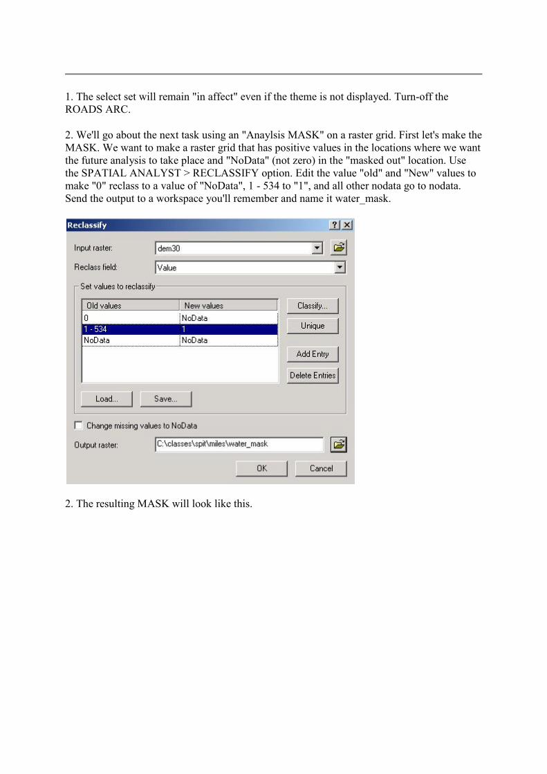
2. We'll go about the next task using an "Anaylsis MASK" on a raster grid. First let's make theMASK. We want to make a raster grid that has positive values in the locations where we wantthe future analysis to take place and "NoData" (not zero) in the "masked out" location. Usethe SPATIAL ANALYST > RECLASSIFY option. Edit the value "old" and "New" values tomake "0" reclass to a value of "NoData", 1 - 534 to "1", and all other nodata go to nodata.Send the output to a workspace you'll remember and name it water_mask.

2. The resulting MASK will look like this.

4. Now use the SPATIAL ANALYST > OPTIONS selection and the GENERAL tab to set theANALYSIS MASK to the new water_mask

3. Use the SPATIAL ANALYST > RASTER CALCULATOR option from the "SpatialAnalyst toolbar" and make a raster calcuation for when the DEM30 < 20 equation test true.

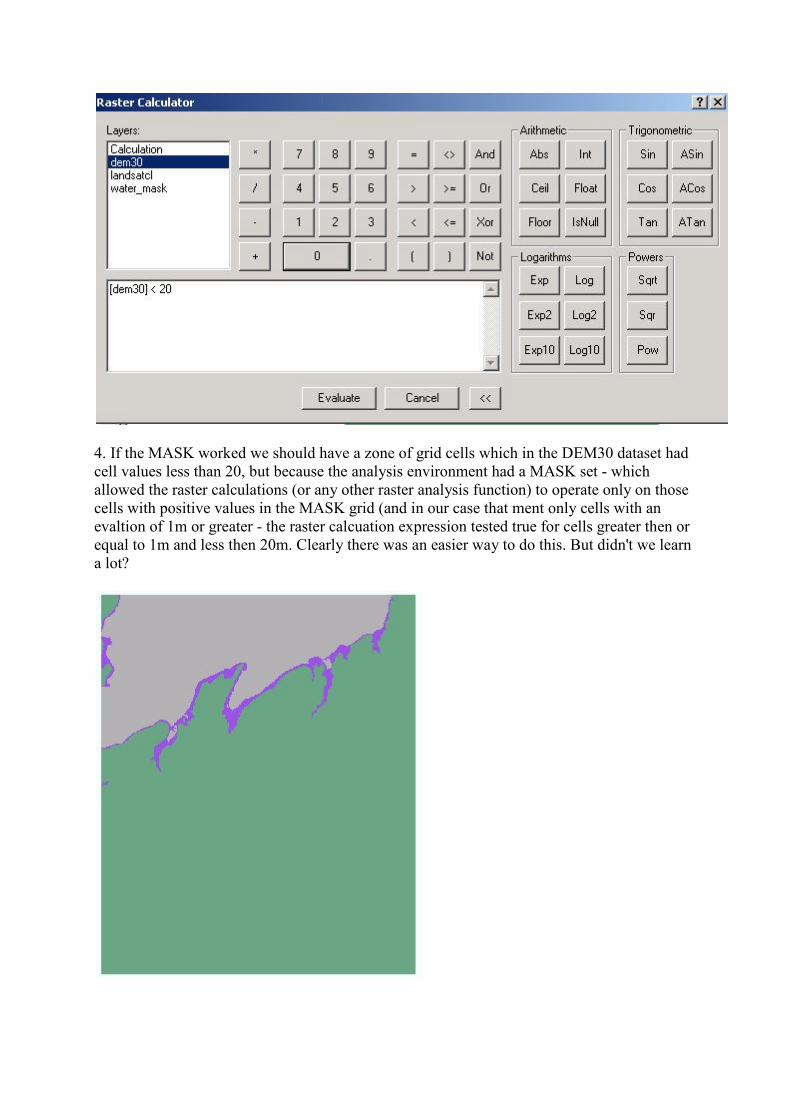
4. If the MASK worked we should have a zone of grid cells which in the DEM30 dataset hadcell values less than 20, but because the analysis environment had a MASK set - whichallowed the raster calculations (or any other raster analysis function) to operate only on thosecells with positive values in the MASK grid (and in our case that ment only cells with anevaltion of 1m or greater - the raster calcuation expression tested true for cells greater then orequal to 1m and less then 20m. Clearly there was an easier way to do this. But didn't we learna lot?

5. Now let's findout what the MEAN elevation is in the coastal zone we've just defined. Usethe SPATIAL ANALYST > ZONAL STATISTICS option to open the Zonal Statistics dialog.Zone dateset will be new grid we calculated (mine is named CALCULATION). TheFIELD in that attribute table for that grid that defines which zone each cell belongs to isnamed VALUE (1 = in the coastal zone, 0 = upland zone). The grid which contains the valueswhich we wish to summarize is DEM30. The Statistic we want is the MEAN, and then weprovide a location on the harddrive for the output table (note that the default is a *.dbf file, I'llname mine coastal_elev_mean)

6. As you can see, the MEAN elevation in my coastal zone is 9.89m. This is calculated from atotal of 5331 cells which have a combined area of 4,797.9 hectacres. It is interesting to notethat the majority of the cells had a value of 5m. If you refresh your ArcCatalog you'll see thatthe table has been written to you workspace.

7. By zooming in on the coastal region and using the option in the symbology for the"Calculation" grid values that equal "1" to have "No Color" I can display the Landsatcl(classified landcover) in the coastal zone. It looks like there is a great deal of "LOCAL"variety. I wonder if the coastal zone is more heterogenious then the uplands. To find out we'llfirst calculate a "FOCAL VARIETY 3X3" analysis on all of the landsatcl dataset - That's a"Neighborhood function" in ArcMAP. SPATIAL ANALYST > NEIGHBORHOOD.

The input data is landsatcl, the field from that grid's attribute table is "L1", the statistic is"variety" the neighborhood I'll define is a 3x3 rectangle of cells, the default cellsize is fine andI'll output the results to my workspace named "class_var".

8. This is descrete data (values of 1, 2, ....9) - you see the neighborhood has is made up of 9cells ( the center plus 8 neighbors) so if all the cells have different landcover values the centercell will have a value of 9. If they are all the same then the value will be 1. Change thesymbology to unique values and pick a color ramp

9. Do again the zonal statistics function again. This time ask for the "MAJORITY" value inthe coastal and upland zones (where "1" in the grid name Calculation = coastal, and "2" =upland). The value raster grid we wish to summarize in this way is the grid I'm named"class_var" (the result of the neighborhood variety function). I'll output my table with thename "lc_zone_majority"

10. It looks like the Upland has a lower variety (3), while the Coastal Zone is higher (4).Makes sense.

1. You remember those roads that we selected which were of type "M" , but also over thegeneral area of the Big Beef Creek DEM30 dataset? Make your display illustrate the twozones we've defined (coastal and upland - ie. the "Calculation" raster dataset) and turn theROADS ARC theme back on. The selected set should still be in affect.

2. Let's use the SPATIAL ANALYST to convert the selected ROADS ARC vectors to theraster format.

3. In the dialog box make your Input features "ROADS ARC", the field in the attribute tableof ROADS ARC that I'll use to identify each road is ROADS-ID, I'll change the cell size to30, and output the results to a grid name "sel_road".

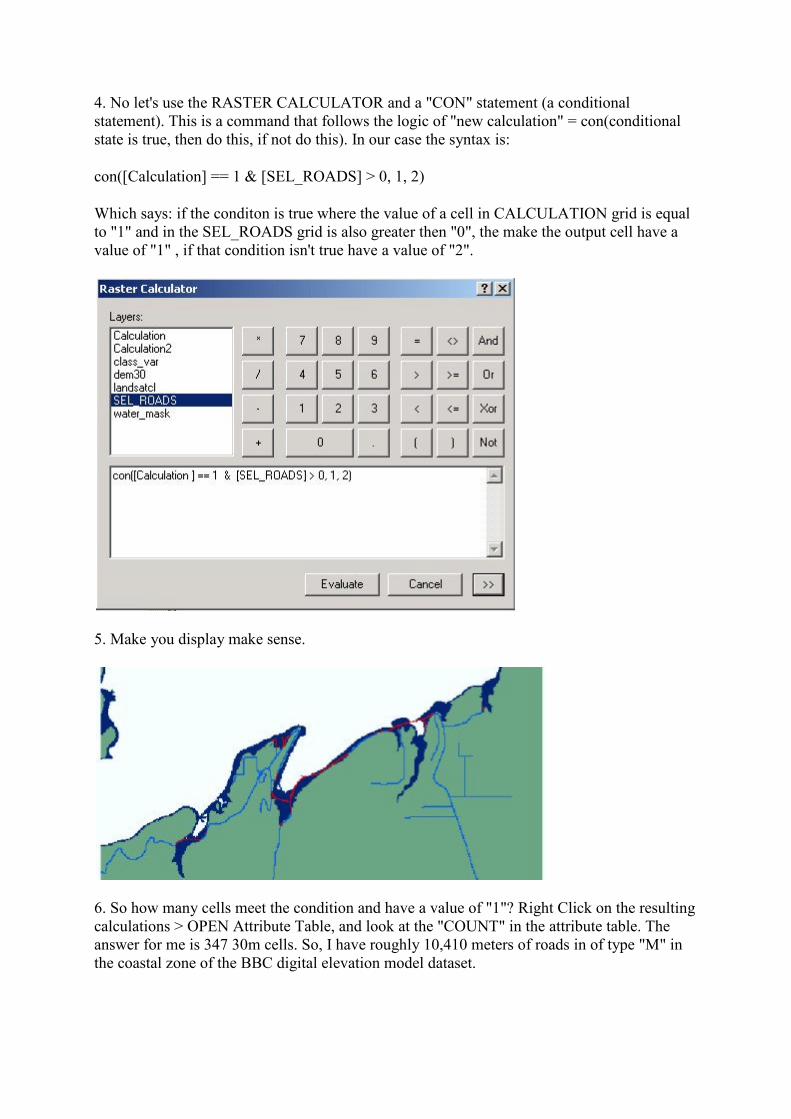
4. No let's use the RASTER CALCULATOR and a "CON" statement (a conditionalstatement). This is a command that follows the logic of "new calculation" = con(conditionalstate is true, then do this, if not do this). In our case the syntax is:

con([Calculation] == 1 & [SEL_ROADS] > 0, 1, 2)

Which says: if the conditon is true where the value of a cell in CALCULATION grid is equalto "1" and in the SEL_ROADS grid is also greater then "0", the make the output cell have avalue of "1" , if that condition isn't true have a value of "2".

5. Make you display make sense.

6. So how many cells meet the condition and have a value of "1"? Right Click on the resultingcalculations > OPEN Attribute Table, and look at the "COUNT" in the attribute table. Theanswer for me is 347 30m cells. So, I have roughly 10,410 meters of roads in of type "M" inthe coastal zone of the BBC digital elevation model dataset.

This was a lot of "stuff". However, it introduced a number of useful functions. It's time to gohome.