selecting optimum location and type of wind … · selecting optimum location and type of wind...
TRANSCRIPT

SELECTING OPTIMUM LOCATIONAND TYPE OF
WIND TURBINES IN ICELAND
May 2012Kristbjörn Helgason
Master of Science in Decision Engineering


SELECTING OPTIMUM LOCATION ANDTYPE OF WIND TURBINES IN ICELAND
Kristbjörn HelgasonMaster of ScienceDecision EngineeringMay 2012School of Science and EngineeringReykjavík University
M.Sc. RESEARCH THESISISSN 1670-8539


Selecting optimum location and type ofwind turbines in Iceland
by
Kristbjörn Helgason
Research thesis submitted to the School of Science and Engineeringat Reykjavík University in partial fulfillment of
the requirements for the degree ofMaster of Science in Decision Engineering
May 2012
Research Thesis Committee:
Dr. Páll Jensson, SupervisorProfessor, Department Head, School of Science and Engineering,Reykjavik University
Dr. Hlynur Stefánsson, Co-SupervisorAssistant Professor, School of Science and Engineering,Reykjavik University
Dr. Ágúst Valfells, Co-SupervisorAssociate Professor, School of Science and Engineering,Reykjavik University
Dr. Hrafnkell Kárason, ExaminerPartner, Summa ehf.

CopyrightKristbjörn Helgason
May 2012

Date
Dr. Páll Jensson, SupervisorProfessor, Department Head, School of Science andEngineering, Reykjavik University
Dr. Hlynur Stefánsson, Co-SupervisorAssistant Professor, School of Science and Engineering,Reykjavik University
Dr. Ágúst Valfells, Co-SupervisorAssociate Professor, School of Science and Engineering,Reykjavik University
Dr. Hrafnkell Kárason, ExaminerPartner, Summa ehf.
The undersigned hereby certify that they recommend to the School of Sci-ence and Engineering at Reykjavík University for acceptance this researchthesis entitled Selecting optimum location and type of wind turbines in Icelandsubmitted by Kristbjörn Helgason in partial fulfillment of the requirementsfor the degree of Master of Science in Decision Engineering.

Date
Kristbjörn HelgasonMaster of Science
The undersigned hereby grants permission to the Reykjavík University Li-brary to reproduce single copies of this research thesis entitled Selectingoptimum location and type of wind turbines in Iceland and to lend or sellsuch copies for private, scholarly or scientific research purposes only.
The author reserves all other publication and other rights in association withthe copyright in the research thesis, and except as herein before provided, nei-ther the research thesis nor any substantial portion thereof may be printed orotherwise reproduced in any material form whatsoever without the author’sprior written permission.

Selecting optimum location and type of wind turbines in Iceland
Kristbjörn Helgason
May 2012
Abstract
In this research study, 48 locations around Iceland are studied along with 47different wind turbines to indicate the potentials of wind power extractionusing every combination of location and turbine.
The historical wind data from the locations are analyzed using the Weibulldistribution and simulated to generate a representative year. Using the powercurves of the 47 turbines, a model is constructed that calculates and com-pares three performance measurements for each turbine at each location.These measurements are: Expected annual energy output (in GWh), capac-ity factor (in % of maximum energy possible to generate) and cost of energy(ce /kWh).
In total, 2256 different combinations of locations and turbines are compared.The combination giving the lowest cost of energy is using a certain 3MWturbine at Garðskagaviti, and that combination is considered to be econom-ically optimal. Additionally, Garðskagaviti is the location giving the bestresults for all the measures mentioned above.
In general, the study reveals relatively high energy output and capacity fac-tors for numerous locations and turbines which indicates that wind power ex-traction could be feasible in Iceland compared to other countries. However,the cost calculations show that the cost per kWh of energy is still too highfor the wind power source to compete with other renewable energy sourcesin Iceland, given the cost assumptions in this study.
Staðar- og tegundarval vindhverfla á Íslandi
Kristbjörn Helgason
Maí 2012
Útdráttur
Í þessu verkefni er skoðuð möguleg hæfni 47 mismunandi gerða vindhverflatil raforkuframleiðslu á 48 ólíkum stöðum á Ísland og mælikvarðar reiknaðirfyrir hverja samsetningu af tegund og staðsetningu.
Söguleg vindgögn eru greind með Weibull drefingu og sú greining notuð tilað herma vind sem gefur dæmigert vind-ár á hverjum stað. Með því að látaþann vind verka á aflferil (e. power curve) hvers vindhverfils er smíðað líkantil að reikna þrjá mælikvarða á hæfni hvers hverfils á hverjum stað. Þessirmælikvarðar eru: vænt árs-orkuframleiðsla (mæld í GWh), nýtingarhlutfall(e. capacity factor, mældur í % af hámarksafli) og kostnaður á kílóvattstundframleiddrar orku (mældur í evru-sentum á kWh).
Samtals eru 2256 ólíkar samsetningar af staðsetningu og vindhverfli bornarsaman. Sú samsetning sem skilar lægstum kostnaði á kWh, af þeim möguleikumsem skoðaðir eru, er að nota vissa gerð 3MW vindhverfils við Garðskagavita.Að auki kemur Garðskagaviti best út við skoðun allra mælikvarðanna.
Almennt sýna niðurstöður verkefnisins hátt nýtingarhlutfall og mikla orkufram-leiðslu fyrir margar staðsetninganna. Það ætti að benda til þess að Íslandhenti vel til vindorkuframleiðslu miðað við önnur lönd. Hins vegar sýnaútreikningar að framleiðslukostnaður á hverja kWh er enn of hár til að vin-dorka geti keppt við aðra orkugjafa á Íslandi, þar sem hann er í öllum tilvikumhærri en söluverð rafmagns hér á landi, m.v. forsendur kostnaðarútreinkninga.

This thesis is dedicated to my late father, Helgi Kristbjarnarson, who opened the world
of science to me and made me the person I am.


vii
Acknowledgements
This thesis would not have been possible without the help and support of a lot of people.
First of all, I am truly thankful to my supervisor, Páll Jensson for his advice and guidanceand for having confidence in me and the project from the very start. His approach toresearch and problem solving has inspired me to become a better researcher.
I would also like to thank my co-supervisors, Ágúst Valfells and Hlynur Stefánsson, fortheir input for getting the project on track. Moreover, they provided me with the necessaryknowledge and techniques, throughout the graduate studies, for me to be able to conductthis kind of research.
My sincerest thanks to Einar Sveinbjörnsson, for taking the time to give me invaluableadvice and guidance through the breezy world of wind observation.
Rán Jónsdóttir, at Landsvrikjun, gave me valuable insight into the wind power sector ofLandsvirkjun for which I am very thankful.
Thanks to Kristján Jónasson, and his research team at the University of Iceland for al-lowing me access to data and their great tool to clean up wind data, saving me hours ofheadache and data manipulation.
Thanks to Magni Þ. Pálsson at Landsnet, for swiftly assisting me anytime I needed.
I am truly grateful to my mother, Sigríður, my mother-in-law, Vilborg, and father-in -law,Leifur, for all their help, time and commitment. Their faith in me helped me to work ashard as I did.
Most of all, I would like to thank my wife and love, Inga María. Without her help anddedication, none of this would have been possible, and without her and our kids, Júlía andJakob, none of this would have been worth doing. You are my inspiration, my best friendsand my biggest supporters.
This work was partly funded by Orkurannsóknarsjóður Landsvirkjunar, for which I amtruly grateful.

viii
ix
Contents
List of Figures xi
List of Tables xii
1 Introduction 1
2 Background and Literature Review 52.1 Wind power planning . . . . . . . . . . . . . . . . . . . . . . . . . . . . 52.2 Wind energy and power . . . . . . . . . . . . . . . . . . . . . . . . . . . 92.3 Modeling . . . . . . . . . . . . . . . . . . . . . . . . . . . . . . . . . . 12
3 Methods 153.1 Data . . . . . . . . . . . . . . . . . . . . . . . . . . . . . . . . . . . . . 153.2 Statistical Modeling of Wind . . . . . . . . . . . . . . . . . . . . . . . . 183.3 Projection of Wind Speed to Higher Altitudes . . . . . . . . . . . . . . . 193.4 Simulation of Wind Speed and Power . . . . . . . . . . . . . . . . . . . 203.5 Energy calculation . . . . . . . . . . . . . . . . . . . . . . . . . . . . . . 213.6 Distance from weather stations to substations . . . . . . . . . . . . . . . 223.7 Cost analysis . . . . . . . . . . . . . . . . . . . . . . . . . . . . . . . . 233.8 Limitations . . . . . . . . . . . . . . . . . . . . . . . . . . . . . . . . . 25
4 Results 274.1 Wind Analysis and Simulation . . . . . . . . . . . . . . . . . . . . . . . 274.2 Annual Energy Output . . . . . . . . . . . . . . . . . . . . . . . . . . . 304.3 Maximum Capacity Factor . . . . . . . . . . . . . . . . . . . . . . . . . 314.4 Minimum Cost of Energy . . . . . . . . . . . . . . . . . . . . . . . . . . 344.5 Comparison to calculations at Búrfell . . . . . . . . . . . . . . . . . . . . 38
5 Conclusions 395.1 Conclusions . . . . . . . . . . . . . . . . . . . . . . . . . . . . . . . . . 395.2 Summary of contribution . . . . . . . . . . . . . . . . . . . . . . . . . . 405.3 Future Research . . . . . . . . . . . . . . . . . . . . . . . . . . . . . . . 41
References 43

x
Appendix
A Wind and Weibull parameters 47
B Turbines 51
C Distance from location to nearest substation 53
D Computer Codes 55
xi
List of Figures
2.1 Trend of turbine prices . . . . . . . . . . . . . . . . . . . . . . . . . . . 14
3.1 A weather station at Skálafell . . . . . . . . . . . . . . . . . . . . . . . . 163.2 Locations of selected weather stations . . . . . . . . . . . . . . . . . . . 163.3 Power curves of all turbines used in the study . . . . . . . . . . . . . . . 173.4 Layout of electricity grid and substations . . . . . . . . . . . . . . . . . . 18
4.1 Top ten locations with the highest annual mean wind speed . . . . . . . . 274.2 Mean wind speeds per month for top 25 stations . . . . . . . . . . . . . . 284.3 Example of a Weibull fit to measurements . . . . . . . . . . . . . . . . . 294.4 Example of measured and simulated wind and its Weibull curve . . . . . . 294.5 Annual energy output for all turbines and locations . . . . . . . . . . . . 304.6 Capacity factors for all turbines at all locations . . . . . . . . . . . . . . . 314.7 Capacity factors of all turbines for the top ten locations . . . . . . . . . . 324.8 Top ten locations with the highest capacity factor . . . . . . . . . . . . . 334.9 Cost of energy for all turbines at all locations . . . . . . . . . . . . . . . 354.10 Cost of energy for all turbines at the top five locations . . . . . . . . . . . 364.11 Top ten locations that give the lowest cost of energy . . . . . . . . . . . . 37

xii

xiii
List of Tables
3.1 Examples of power law exponents . . . . . . . . . . . . . . . . . . . . . 19
4.1 Results for different turbines at Búrfell . . . . . . . . . . . . . . . . . . . 38
A.1 Weibull parameters and measured mean wind . . . . . . . . . . . . . . . 47
B.1 Turbine parameters and power in kW at 1-11 m/s . . . . . . . . . . . . . 51B.2 Turbine power output in kW at 12-28 m/s . . . . . . . . . . . . . . . . . 52
C.1 Distance from weather stations to nearest substation . . . . . . . . . . . . 53

xiv

1
Chapter 1
Introduction
Like most countries, Iceland is faced with the challenge of how to meet the foreseeableincrease in energy demand in the world. According to the International Energy Agency’sReference Scenario, global primary energy demand is expected to grow by 40% in theyears between 2007 and 2030.
Iceland has its own energy demand forecast for the years 2011-2050, made by The Na-tional Energy Authority (Orkustofnun) in 2011. According to the forecast, primary energydemand will have increased by 7% in 2015, and by 94% in the next forty years. Energydemand is in close relation to changes in the volume of industrial production as well aspopulation development. Moreover, usage can be expected to change and go hand-in-handwith progress in technology.
Iceland’s energy use per capita is among the highest in the world, according to The Na-tional Energy Authority. Although the share of renewable energy sources in Iceland ex-ceeds most other countries, the need is extreme to guarantee responsible and sustainableexploitation of those sources. There is no single solution to meeting the energy demand inIceland. Instead, a combination of solutions is probably the answer. The interests of futuregenerations need also to be kept in mind in the implementation of new energy policies,and the environment has to be left as unspoiled as possible. Therefore, more diversifiedusage of renewable energy sources in Iceland needs to be studied.
Wind power is currently one of the most cost efficient renewable energy sources availableand the one of few that are available anywhere in the world, although some locations aremore suitable for wind power production than other. The deciding factors on how muchpower can be produced at any location are the strength and distribution of the wind profileand how it matches to a particular wind turbine generator.
2 Selecting optimum location and type of wind turbines in Iceland
When choosing a location for a wind turbine, the wind profile of each prospective locationneeds to be studied, as well as which type of turbine best matches that wind profile. Thisprocess needs to be based on analysis of the stochastic element of wind for each locationand the possible energy output of each turbine considered.
Each wind turbine type has a unique power curve which represents the turbine’s optimalwind speed and the range of wind speeds that can drive the turbine. By comparing themean wind speed of a location with a power curve, one can get a rough estimate of the po-tential power production at that particular location for that turbine. However, as the powercurve is non-linear and wind is a highly stochastic element, the frequency distribution ofthe wind has to be taken into account to get a realistic estimate.
In this study the monthly wind profile of 48 different locations in Iceland are analyzed.This provides the necessary parameters to be able to conduct a simulation of future winddata for these locations. This simulated wind is run through 47 different wind turbinepower curves.
Three performance measures are calculated for all turbines at each location:
- The amount of energy that each turbine is expected to produce annually.
- The capacity factor of each turbine, which gives the percentage of maximum pos-sible energy generated by a turbine at a certain location. This indicates how well aturbine matches the location’s wind profile.
- The cost of energy in cente /kWh, calculated as the annual payment of the totalcost of each turbine at each location divided by the annual energy production. Thisindicates which combination generates maximum energy relative to the setup andoperating costs.
By finding the setup leading to the minimum cost of energy for each location, an econom-ically optimal wind turbine is identified for each location. Thereby, the overall optimalpair of location and wind turbine can be identified.
The weather data used in this study were collected by The Icelandic Meteorology Officein the years 1998 to 2010. All locations selected to be included in the study have historicaldata of nine years or more and altitude of less than 330 meters above sea level.
Turbine data from most leading turbine manufacturers are retrieved, mainly from a datasetput together by the British Wind Power Program (The WindPower Program, n.d.). Thedata retrieved is combined into a database of 47 turbines that are used in this study.
Kristbjörn Helgason 3
Most of the largest wind parks in the world today are located off-shore. It has considerableadvantages over on-shore locations, because of more stable wind and possibilities of lessenvironmental impact. However, off-shore wind parks near Iceland are not likely to beconstructed in near future, as costs are far higher than onshore, and not enough researchhas been done on their endurance and performance around Iceland. Therefore, this studywill focus on on-shore locations.
Aim and objective
The aim of this study is to find optimum locations for wind turbines in Iceland and identifythe optimum type of turbine to be used at each location. The objective is to build a modelthat calculates and compares performance measures of different combinations of locationsand wind turbine types. The model identifies an optimum pair of wind turbine locationand type out of the combinations considered. The optimum pair of location and type isconsidered to be the one that has the lowest cost of energy, based on simulation derivedfrom historical wind data.
Additionally, the outcome of this study is compared to an extensive energy output esti-mation for the Búrfell area, which was conducted for Landsvirkjun (The National PowerCompany in Iceland) in 2011.
Motivation
In recent years, discussion about reduction in usable energy production options in Icelandhas increased. There is not a general agreement on how much is left of usable hydropower,while most agree that geothermal energy needs to be studied further to determine its sus-tainability. Therefore, continuing research of other renewable energy sources in Icelandsuch as wind energy is of great importance.
In the process of choosing the most suitable location and type of wind turbine to be setup,many variables need to be considered. Each type of wind turbine has its specific windspeed working range, presented with the turbine’s power curve. The location with thehighest mean wind speed need not be the one generating the most energy on an annualbasis and due to different power curves, the largest turbine might not even be the one thatgenerates the most energy. However, the largest turbine can be assumed to be the mostexpensive one as the cost can be roughly estimated to increase linearly with the rotordiameter of the turbine.

4 Selecting optimum location and type of wind turbines in Iceland
Earlier studies on production of wind power in Iceland use either semi-annual or annualwind speed averages to estimate potential power at the location studied. Moreover, onlyone specific turbine is used to calculate the expected energy output in each of the studies,without considering the different characteristics of turbines.
Seasonal fluctuations in the wind make annual average wind speeds an imprecise para-meter to base an energy calculations on. As an example, annual average wind speed canbe high while certain months have mean wind speeds outside of the working wind speedrange of a particular turbine and therefore leading to low efficiency of the turbine.
In this study the wind is analyzed and simulated on monthly basis which reveals largedeviations in wind speeds between months. It also incorporates the difference of 47 tur-bines and estimates the cost and capacity factor of each one, giving an indication of whichturbine might be the most suitable at each location.
Outline of the thesis
Chapter 2 describes the background of wind power and the state of the art. Literature isreviewed, both recent publications on wind power as well as classical definitions of windand wind power measurements.
Chapter 3 describes the methods and data used in this study. The first part describes thedata and the second and third part describe statistical methods for wind modeling. Nextthree parts describe methods used for simulation, energy calculation and cost analysis.Some limitations to the study are also listed.
Chapter 4 presents the results of the study. First, the results of the wind modeling andsimulation are presented. Secondly, annual energy output estimates are presented. Thelast part presents the main results of this study, the efficiency and cost of energy for eachlocation and turbine.
Chapter 5 concludes the work of this study, discusses the meaning of the results andportraits the most interesting findings. Moreover, a short summary of the contribution ofthe study is given and some future research suggested.
5
Chapter 2
Background and Literature Review
2.1 Wind power planning
Wind measurements and modeling
The deciding factors on the magnitude of the wind power that can be produced at anylocation, are the strength and distribution of the wind profile and how it matches to aparticular wind turbine generator. Therefore, all wind power planning is based on windmeasurements. This is for example stated in a recent study of the wind energy potentialin Iran, where a team of researchers led by A. Keyhani analyzed long-term wind data onmonthly basis to get an estimate of potential energy at a certain location (Keyhani et al.,2010).
Wind was first statistically modeled as a discrete random variable in 1951 (Sherlock,1951), by using the Gamma distribution. In recent years the two parameter Weibull distri-bution has emerged as the most commonly used density function to model wind as it hasbeen found to make a good fit to wide selection of wind data (Celik, 2004; Lun & Lam,2000; Yeh & Wang, 2008).
The Weibull distribution, named after the Swedish scientist Waloddi Weibull, was firstapplied in 1933 (Rosin & Rammler, 1933). The distribution can be applied in various cir-cumstances to describe the frequency of events, wind being one thereof. Keyhani and col-leagues even go as far as stating that the Weibull distribution “is widely accepted for eval-uating local wind load probabilities and can be considered almost a standard approach”(Keyhani et al., 2010).
6 Selecting optimum location and type of wind turbines in Iceland
Automatic weather observations have been made in Iceland since 1990 by the IcelandicMeteorology Office. In the current form of wind measurements, mean wind speed isrecorded every ten minutes in more than 200 places around the country, as well as thehighest gust speed in that same period (Icelandic Meteorological Office, n.d.).
All the automatic observations are taken at approximately ten meters above ground, whilewind turbines operate at much higher altitudes. The projection of wind speed to higheraltitudes is a well studied and documented process. The most widely used formula for theprojection is the power law, described in i.e. (J.F. Manwell & Rogers, 2002) as
V (z)
V (zR)=
(z
zR
)a(2.1)
where V (z) is the wind speed at height z, V (zR) is the measured wind speed at height zR,and a is the power law exponent, describing the terrain surface and stability of the air. Theearly works on the formula date back to 1968 where it is showed that a = 1/7 ≈ 0.14,can be reasoned to be a typical value of the exponent (Schlichting, 1968).
Some studies in Iceland on wind speed varying with height have revealed values of thepower law exponent for certain locations (Arason, 1998; Sigurðsson et al., 1999; J. Blön-dal et al., 2011). The calculated values of the exponent range mainly between 0.08-0.16.Recent, unpublished studies by G. N. Petersen at Keflavik airport using weather balloons,show that the value of a=1/7 is reasonable for the area. Preliminary results of anotherrecent unpublished study at the Búrfell area show a value near a = 0.12 for the exponent.That study uses recent and extensive wind measurements at different heights.
Wind power research in Iceland
Wind power has never been industrially extracted in Iceland, although some small turbineshave been set up, mostly for private use. Despite that fact, some conditions such asmean wind speed and land availability are favorable in Iceland for large scale wind plants.The low cost of other available power sources, such as hydro and geothermal power,is probably the primary reason for the lack of effort in wind power usage in Iceland.However, in recent years the interest in wind power in Iceland has increased, followingmore emphasis on diversity in power production and sustainable use of natural powersources.

Kristbjörn Helgason 7
In a report from 2009 for the Ministry of Industry, some of the potentials of harvestingwind power in Iceland were identified and listed. The main potentials for Iceland werefound to be (Sigurjónsson, 2009):
- Generate wind power in large scale to maximize efficiency and buildup of waterreservoirs
- Construct small wind power turbines, where applicable, to lower the need of longdistance transporting of electricity, thereby minimizing distribution costs
- Construct large scale wind power plants for electricity export, if plans of a subma-rine cable to Europe follow through
Landsvirkjun plans to construct two wind turbines in 2012 for research purposes. Theturbines will be located near the hydro power plant at Búrfell, where extensive energyoutput estimation has been performed (Petersen & Björnsson, 2011). One of its aims isto research the possibilities of wind power to increase the efficiency and buildup of waterreservoirs. That way more power could be extracted from the hydro power plants, pro-viding base load electricity despite the stochastic behavior of wind power. (Landsvirkjun,2012).
As these plans indicate, Landsvirkjun is increasing its emphasis on wind energy. At thecompany’s Autumn meeting in 2011, the executive vice president of Research and De-velopment, stated that wind is a realistic option with rising electricity prices, and that itmight become competitive with hydro and geothermal power within ten years. In addi-tion, if a submarine cable to Europe would become a realistic possibility in near future,it could create additional opportunities for utilization of wind power and development ofthe electricity system (Ó. G. Blöndal, 2011).
In the years 2010 and 2011, The Icelandic Meteorological Office and The University ofIceland collaborated in a wind power research for locations all around Iceland. The groupprojected wind speeds around Iceland up 90 meters and interpolated between locations.The correlation between locations was calculated in order to find places in which windturbines can be installed to maximize total runtime of combined power plants. The cal-culations were based on mean winds of summer and winter from long-term wind data.Data for a few wind turbines were aggregated into one mean wind turbine, of class IEC1a (J. Blöndal et al., 2011). In general, their findings show that overall efficiency can beincreased by locating wind turbines in several different, uncorrelated locations.
A part of their study was to build a tool to automatically clean up corrupted wind data.When failures occur in automatic wind monitors, either wrong measurements are recorded
8 Selecting optimum location and type of wind turbines in Iceland
or measurements are missing. One of the reasons behind such deviations is that electricalfields can build up in the monitors and corrupt the measurements. Icing can also influencemonitors, as well as other conventional failures in their mechanism. Due to the frequencyof these errors, a tool for automatic cleanup process, as the one the research team con-structed, is valuable for further use of wind data (J. Blöndal et al., 2011).
The process of matching wind turbines with specific wind profile is important to max-imize the possible extraction of energy. One of few published papers on the topic isAbul’Wafa’s paper about matching wind turbines with certain wind profile for decidingon wind farm location in Egypt. In his study, he presented a method for matching windturbine generators to a site using turbine performance index in conjunction with minimumdeviation ratio between the rated speed of wind turbine and optimal speed, resulting inminimum cost of energy (Abul’Wafa, 2011).
Specialized computer programs are widely used to estimate energy output of a wind tur-bine at a certain location. One of the best known in Europe is a program called WAsP(Mortensen & Laboratory, 2007). The program uses, the Weibull distribution to modelwind, along with more detailed topography information and energy conversion calcula-tions. It is capable of giving extensive energy calculations but it is proprietary with highlicense fees.
In 2011 The Icelandic Meteorology Office conducted an extensive energy study on theBúrfell area for Landsvirkjun, as the company is planning to install an experimental windturbine in the area in 2012. The study uses WAsP and the result is a detailed estimationof possible energy generation at the location but the study uses only one type of turbine.The research shows that the power density at certain locations in the area can be expectedto be as high as 975 W/m2 and a high capacity factor can be achieved using the turbinestudied (Petersen & Björnsson, 2011).
In 1985, the University of Iceland constructed a wind turbine in Grímsey, a small inhabitedisland in the North of Iceland, for the purposes of heating water for central heating. Theturbine blades were damped by a hydraulic brake which again heated water with friction,that was used to heat up buildings in the proximity. The turbine broke down shortly afterit was constructed and has not been used since. The turbine still stands, although it isin poor condition and will probably never run again. Two reports from 1985 and 2003show that the use of wind power for central heating in Grímsey would be cost-effective.One of the main conclusions of the latter report is to state the importance of immediatelyconducting a technical review on the synergy of a diesel power generator and a windturbine in Grímsey (Nefnd um sjálfbært orkusamfélag í Grímsey, 2003).
Kristbjörn Helgason 9
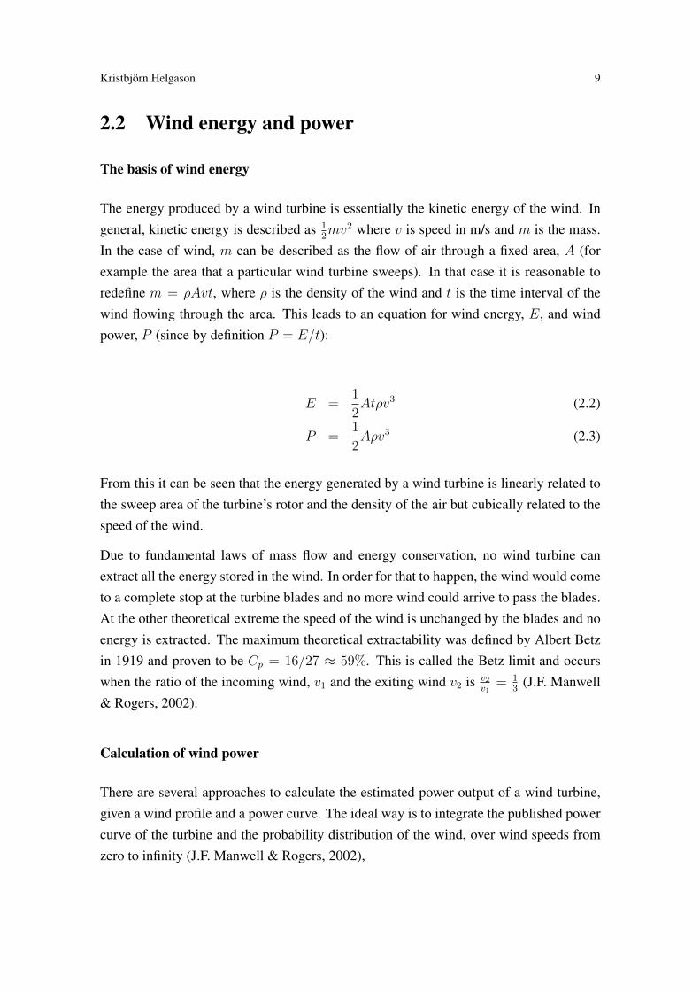
2.2 Wind energy and power
The basis of wind energy
The energy produced by a wind turbine is essentially the kinetic energy of the wind. Ingeneral, kinetic energy is described as 1
2mv2 where v is speed in m/s and m is the mass.
In the case of wind, m can be described as the flow of air through a fixed area, A (forexample the area that a particular wind turbine sweeps). In that case it is reasonable toredefine m = ρAvt, where ρ is the density of the wind and t is the time interval of thewind flowing through the area. This leads to an equation for wind energy, E, and windpower, P (since by definition P = E/t):
E =1
2Atρv3 (2.2)
P =1
2Aρv3 (2.3)
From this it can be seen that the energy generated by a wind turbine is linearly related tothe sweep area of the turbine’s rotor and the density of the air but cubically related to thespeed of the wind.
Due to fundamental laws of mass flow and energy conservation, no wind turbine canextract all the energy stored in the wind. In order for that to happen, the wind would cometo a complete stop at the turbine blades and no more wind could arrive to pass the blades.At the other theoretical extreme the speed of the wind is unchanged by the blades and noenergy is extracted. The maximum theoretical extractability was defined by Albert Betzin 1919 and proven to be Cp = 16/27 ≈ 59%. This is called the Betz limit and occurswhen the ratio of the incoming wind, v1 and the exiting wind v2 is v2
v1= 1
3(J.F. Manwell
& Rogers, 2002).
Calculation of wind power
There are several approaches to calculate the estimated power output of a wind turbine,given a wind profile and a power curve. The ideal way is to integrate the published powercurve of the turbine and the probability distribution of the wind, over wind speeds fromzero to infinity (J.F. Manwell & Rogers, 2002),
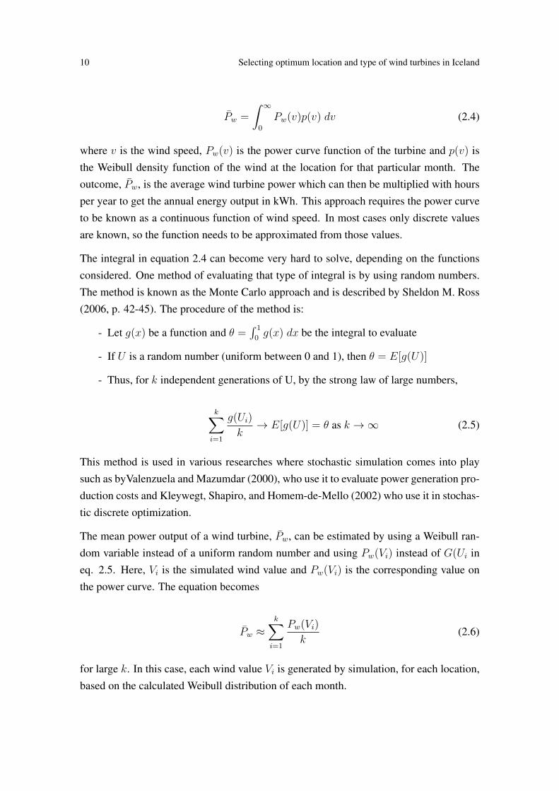
10 Selecting optimum location and type of wind turbines in Iceland
Pw =
∫ ∞0
Pw(v)p(v) dv (2.4)
where v is the wind speed, Pw(v) is the power curve function of the turbine and p(v) isthe Weibull density function of the wind at the location for that particular month. Theoutcome, Pw, is the average wind turbine power which can then be multiplied with hoursper year to get the annual energy output in kWh. This approach requires the power curveto be known as a continuous function of wind speed. In most cases only discrete valuesare known, so the function needs to be approximated from those values.
The integral in equation 2.4 can become very hard to solve, depending on the functionsconsidered. One method of evaluating that type of integral is by using random numbers.The method is known as the Monte Carlo approach and is described by Sheldon M. Ross(2006, p. 42-45). The procedure of the method is:
- Let g(x) be a function and θ =∫ 1
0g(x) dx be the integral to evaluate
- If U is a random number (uniform between 0 and 1), then θ = E[g(U)]
- Thus, for k independent generations of U, by the strong law of large numbers,
k∑i=1
g(Ui)
k→ E[g(U)] = θ as k →∞ (2.5)
This method is used in various researches where stochastic simulation comes into playsuch as byValenzuela and Mazumdar (2000), who use it to evaluate power generation pro-duction costs and Kleywegt, Shapiro, and Homem-de-Mello (2002) who use it in stochas-tic discrete optimization.
The mean power output of a wind turbine, Pw, can be estimated by using a Weibull ran-dom variable instead of a uniform random number and using Pw(Vi) instead of G(Ui ineq. 2.5. Here, Vi is the simulated wind value and Pw(Vi) is the corresponding value onthe power curve. The equation becomes
Pw ≈k∑i=1
Pw(Vi)
k(2.6)
for large k. In this case, each wind value Vi is generated by simulation, for each location,based on the calculated Weibull distribution of each month.
Kristbjörn Helgason 11
Wind Power Density
Wind power density (WPD) is a measure of the kinetic power available per square meterfor certain wind speed. It is calculated by dividing the wind power, P , by the ares, A.This gives a measure which is only related to the wind speed, v, and the density of air,ρ, and is therefore a useful way to estimate the power available in the wind at a certainlocation.
WPD =P
A=
1
2ρv3 (2.7)
In 2004, A. N. Celik showed how to use the Weibull distribution to estimate the meanpower density when he used the measure to show that a site in Southern Turkey pre-sented poor wind characteristics. Moreover, he showed that the Weibull distribution pro-vides better power density estimations than the more simple Rayleigh distribution (Celik,2004).
Wind locations are classified by the American Wind Energy association (AWEA) ac-cording to its wind power density. “Areas designated as class 4 or greater are generallyconsidered to be suitable for most wind turbine applications” (J.F. Manwell & Rogers,2002, p. 67). Those sites show average wind speed of around 7.0-7.5 m/s at an altitude of50 meters (J.F. Manwell & Rogers, 2002; AWEA - Wind Energy FAQ, n.d.).
Capacity factor
One of the most informative measures of how efficiently a wind turbine is functioningat a specific location is the Capacity factor (CF ). It is defined as the ratio of the energyactually produced by a turbine at a given site and the maximum energy that the specificturbine can produce. Thus,
CF =Pwt
PRt=EyearER
(2.8)
where Pw is the mean power produced, PR is the rated power of the turbine, t is anygiven time interval, Eyear is the mean energy produced annually and ER, is the maximumenergy that the specific turbine can produce annually. (J.F. Manwell & Rogers, 2002, p.63)
12 Selecting optimum location and type of wind turbines in Iceland
The Capacity factor is used in many cases where efficiency of turbines are compared suchas by Celik (2003) and Chang and Tu (2007). Typical wind power capacity factors havebeen shown to be in the range 20-40%.
2.3 Modeling
Simulation
To determine an energy output of a wind turbine, some values of future wind speeds areneeded. One way to estimate future wind speed is by simulating wind values from param-eters based on statistical modeling of historical data from a particular location.
Values from a known probability density function (e.g. the Weibull function) can besimulated using, for example, the inverse transform method as described in Rubinsteinand Melamed (1998) and Ross (2006). Mathematical programming languages, such asMatlab or R, have a built-in Weibull generating function, based on their random numbergenerator, which is the approach used by many researchers.
The mean of the simulated values needs to approximate the mean of the historical data.Therefore, many simulation runs are needed for each set of parameters. One method fordetermining the number of simulation runs needed is described by Sheldon M.Ross. Helets S denote the standard deviation of the generated values, k the number of simulationsand determines d as the acceptable standard deviation of the estimator. The method ofdetermining k is to generate simulated values and check each time if S/
√k < d. The
estimate of the mean is then given by X =∑k
i=1Xi/k (Ross, 2006).
One method of reducing k, the number of iterations, is using Antithetic variables (Ross,2006). The method is based on reducing the variance of the estimator by using negativelycorrelated random numbers with the inverse transform method of simulation. The methodis described as:
1. Generate a random number U and use it to generate a random variable X usinginverse transform.
2. Generate a new X using the random number 1− U .
3. Repeat 1 and 2, n times.
4. The mean of the X’s is the estimator for the expected value of the random variable.
Kristbjörn Helgason 13
Cost analysis
The European Wind Energy Association (EWEA) is one of the leading organization ingathering data on cost of wind energy setups. The association regularly publishes factsheets on the development of different cost factors, setting benchmarks for prices in theindustry. According to their publication, capital costs of wind energy projects are dom-inated by the cost of the wind turbine. In 2006, the mean cost per kW of installed windpower capacity was from around e 1000/kW to e 1350/kW, although differing somewhatbetween countries. (EWEA, 2009a).
In recent years, the cost of wind turbines has dropped significantly following technicalprogress in the production as well as increase in supply and competition. The BloombergCorporation calculates a semi-annual Wind Turbine Price Index (WTPI) that reflects theprices of the latest turbine contracts. The latest edition reports that utility-scale windpower equipment prices hit a new low in the second half of 2011 and “contracts signedin the second half of 2011 for 2013 delivery fell to e 0.91m/MW ($1.21m/MW), down4% from six months earlier and well off their five-year high of e 1.21m/MW in 2009”.(Bloomberg, n.d.)
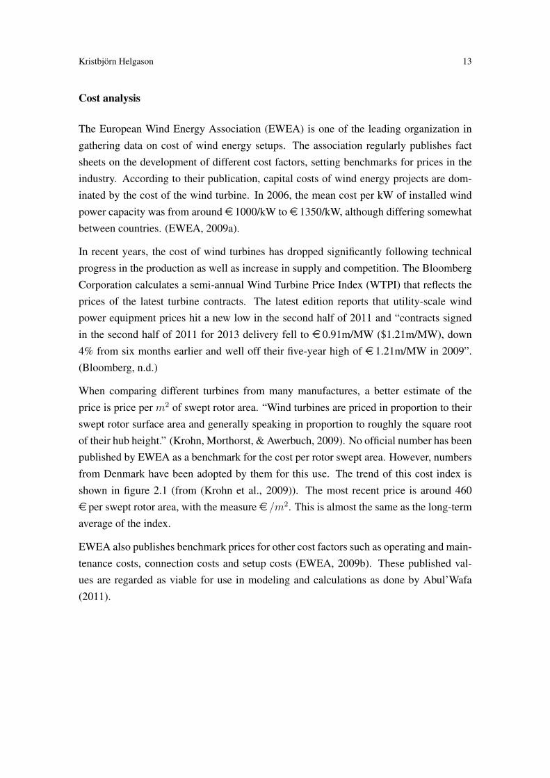
When comparing different turbines from many manufactures, a better estimate of theprice is price per m2 of swept rotor area. “Wind turbines are priced in proportion to theirswept rotor surface area and generally speaking in proportion to roughly the square rootof their hub height.” (Krohn, Morthorst, & Awerbuch, 2009). No official number has beenpublished by EWEA as a benchmark for the cost per rotor swept area. However, numbersfrom Denmark have been adopted by them for this use. The trend of this cost index isshown in figure 2.1 (from (Krohn et al., 2009)). The most recent price is around 460e per swept rotor area, with the measure e /m2. This is almost the same as the long-termaverage of the index.
EWEA also publishes benchmark prices for other cost factors such as operating and main-tenance costs, connection costs and setup costs (EWEA, 2009b). These published val-ues are regarded as viable for use in modeling and calculations as done by Abul’Wafa(2011).
14 Selecting optimum location and type of wind turbines in Iceland
THE ECONOMICS OF WIND ENERGY42
IMPROVEMENT IN EFFICIENCY The development of electricity production ef! ciency, measured as the annual energy production per square metre of swept rotor area (kWh/m2) at a speci! c refer-ence site, has improved signi! cantly in recent years owing to better equipment design.
Taking into account the issues of improved equipment ef! ciency, improved turbine siting and higher hub height, overall production ef! ciency has increased by 2-3% annually over the last 15 years.
The swept rotor area, as we have already stated, is a better indicator of the production capacity of a wind turbine than the rated power of the generator. Also, the costs of manufacturing large wind turbines are roughly proportional to the swept rotor area. In the context of this paper, this means that when we (correctly) use rotor areas instead of kW installed as a measure of turbine size, we would see somewhat smaller (energy) productivity increases per unit of turbine size and a larger increase in cost effective-ness per kWh produced.
Figure 1.15 shows how these trends have affected investment costs as shown by the case of Denmark, from 1989 to 2006. The data re" ects turbines installed in the particular year shown (all costs are
converted to #2006 prices) and all costs on the right axis are calculated per square metre of swept rotor area, while those on the left axis are calculated per kW of rated capacity.
The number of square metres covered by the turbine’s rotor – the swept rotor area - is a good indicator of the turbine’s power production, so this measure is a relevant index for the development in costs per kWh. As shown in Figure 1.15, there was a substantial decline in costs per unit of swept rotor area in the period under consideration, except during 2006. So from the late 1990s until 2004, overall investments per unit of swept rotor area dropped by more than 2% per annum, corresponding to a total reduction in cost of almost 30% over the 15 years. But this trend was broken in 2006, when total investment costs rose by approximately 20% compared to 2004, mainly due to a signi! cant increase in demand for wind turbines, combined with rising commodity prices and supply constraints. Staggering global growth in demand for wind turbines of 30-40% annually, combined with rapidly rising prices of commodities such as steel, kept wind turbine prices high in the period 2006-2008.
Looking at the cost per rated capacity (per kW), the same decline is found in the period from 1989 to 2004, with the exception of the 1,000 kW machine in
Source: Risø DTU
1,200
1,000
800
600
400
200
0
/kW
Price of turbine per kW
Other costs per kW
Total cost per swept m2
600
500
400
300
200
100
0
per
sw
ept
roto
r ar
ea
1989 1991 1993 1995 1997 2001 2004 2006
Year of installation
150 kW 225 kW300 kW
500 kW600 kW
1,000 kW
2,000 kW
FIGURE 1.15: The development of investment costs from 1989 to 2006, illustrated by the case of Denmark.
Right axis: Investment costs divided by swept rotor area (!/m2 in constant 2006 !). Left axis: Wind turbine capital costs (ex works) and other costs per kW rated power (!/kW in constant 2006 !).
Figure 2.1: Trend of turbine prices in Denmark
Cost of transport of energy to the grid
All major electricity transmission lines in Iceland are owned and operated by Landsnet,a company owned by the state and some municipalities and operates under a concessionarrangement. The electrical grid consists of 72 substations that connect the transmissionlines that distribute on either 33kV, 66kV, 132 kV or 220 kV voltage. With increasingheavy industry in Iceland, the electrical grid in the vicinity of the industry has been forti-fied. This industry has accumulated in the South-West and the East of the country. As aresult, the transmission lines and substations in these areas are most dense and powerful(Landsnet, 2011). Tariffs for transmission and ancillary services are published annuallyand are available online (Landsnet, 2012b).
The price of connecting the wind turbine to the grid is directly related to its distancefrom the nearest substation. According to Landsnet, the cost per kilometer of 132kVtransmission lines is approximately 240, 000 e /km (100 mISK/2.6km). However 33kVline suffices for transmission of power below 10MW. The cost of 33kV is estimated to be1/3 of that of 132kV or approximately 80, 000 e /km (Landsnet | Kostnaður, n.d.).

15
Chapter 3
Methods
This chapter starts by describing the data used in this study, then covers the methods usedand ends on discussing some of the limitations of this study.
3.1 Data
3.1.1 Wind Data
This study uses data from weather stations located at altitudes below 330 meters abovesea level that can supply at least nine years of measured data. This leads to a selectionof 48 locations out of the 145 locations considered. All data were collected in the years1998-2010.
Weather stations at more than 400 meters (including the turbine tower) are more suscep-tible to icing which reduces production, and are in general harder to access. Figure 3.1shows a typical weather station at high altitude where icing has occurred. Using onlylocations with more than nine years of history reduces the risk of unusual periods in windmeasurement overly affecting the results.
Figure 3.2 shows a map of the selected locations used in this study.
Use of raw weather data from a recent study made at the University of Iceland, was kindlypermitted by the researchers, as well as access to a Matlab code to clean up the data(J. Blöndal et al., 2011). In this study, the code is run on the raw data from each selectedweather station and the cleaned values are imported into R-programming language forfurther modeling.

16 Selecting optimum location and type of wind turbines in Iceland
Figure 3.1: A weather station at Skálafell, at altitude 771 m
Figure 3.2: Locations of selected weather stations
Kristbjörn Helgason 17
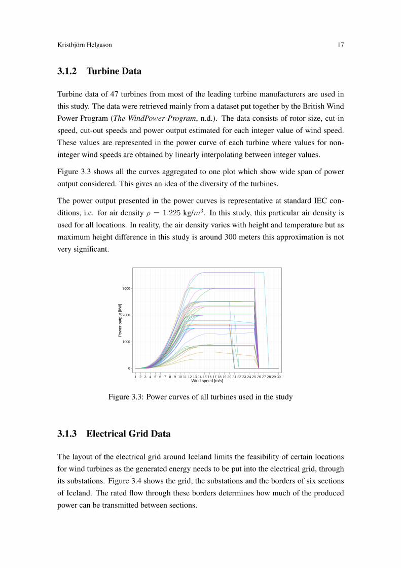
3.1.2 Turbine Data
Turbine data of 47 turbines from most of the leading turbine manufacturers are used inthis study. The data were retrieved mainly from a dataset put together by the British WindPower Program (The WindPower Program, n.d.). The data consists of rotor size, cut-inspeed, cut-out speeds and power output estimated for each integer value of wind speed.These values are represented in the power curve of each turbine where values for non-integer wind speeds are obtained by linearly interpolating between integer values.
Figure 3.3 shows all the curves aggregated to one plot which show wide span of poweroutput considered. This gives an idea of the diversity of the turbines.
The power output presented in the power curves is representative at standard IEC con-ditions, i.e. for air density ρ = 1.225 kg/m3. In this study, this particular air density isused for all locations. In reality, the air density varies with height and temperature but asmaximum height difference in this study is around 300 meters this approximation is notvery significant.
0
1000
2000
3000
1 2 3 4 5 6 7 8 9 10 11 12 13 14 15 16 17 18 19 20 21 22 23 24 25 26 27 28 29 30Wind speed [m/s]
Pow
er o
utpu
t [kW
]
Figure 3.3: Power curves of all turbines used in the study
3.1.3 Electrical Grid Data
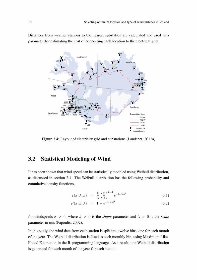
The layout of the electrical grid around Iceland limits the feasibility of certain locationsfor wind turbines as the generated energy needs to be put into the electrical grid, throughits substations. Figure 3.4 shows the grid, the substations and the borders of six sectionsof Iceland. The rated flow through these borders determines how much of the producedpower can be transmitted between sections.
18 Selecting optimum location and type of wind turbines in Iceland
Distances from weather stations to the nearest substation are calculated and used as aparameter for estimating the cost of connecting each location to the electrical grid.
SOG
HRA
SIG BUR
PRE
SUL VAF
HAM
BRE
GEH
SVA
FIT
BLA
KRA RAN
LAV
LAX
VAR
TEH
HOL
HRY
GED
HRU
GLE
MJO
VAT
VEG
AND
AKR
SAU
DAL
KOP
HUS
KEL
BRD
BOL
ISA
VOG GRU OLA
SEL TOR
FLU
HEL HVO
RIM
VES
ESK NSK
SEY EYV
LAG
VOP
FAS FLJ
REY
RAU
LIN
KOL HNO OLD
A12
Northeast
Northwest
Southeast
West
Southwest
South
220 kV132 kV66 kV
Transmision lines
33 kV
Industrial usersSubstations
STU
HVE
NES KOR
Figure 3.4: Layout of electricity grid and substations (Landsnet, 2012a)
3.2 Statistical Modeling of Wind
It has been shown that wind speed can be statistically modeled using Weibull distribution,as discussed in section 2.1. The Weibull distribution has the following probability andcumulative density functions,
f(x;λ, k) =k
λ
(xλ
)k−1e−(x/λ)
k
(3.1)
F (x; k, λ) = 1− e−(x/λ)k (3.2)
for windspeeds x > 0, where k > 0 is the shape parameter and λ > 0 is the scale
parameter in m/s (Papoulis, 2002).
In this study, the wind data from each station is split into twelve bins, one for each monthof the year. The Weibull distribution is fitted to each monthly bin, using Maximum Like-lihood Estimation in the R-programming language. As a result, one Weibull distributionis generated for each month of the year for each station.
Kristbjörn Helgason 19
3.3 Projection of Wind Speed to Higher Altitudes
Wind speed measurements are projected up to the tower height of each turbine using thepower law shown in equation 2.1.
The height, z, at which the turbine operates (height of tower) is normally at least as highas the diameter of the turbine’s rotor (J.F. Manwell & Rogers, 2002). Therefore thisstudy projects wind speed up to different height for each turbine i, that height being:zi = rotor_diameteri
The power law exponent, a, needs to be determined for each location using measurementsmade at different altitudes. As detailed in section 2.1, research in Iceland have revealedvalues for the exponent mainly ranging from 0.08-0.16. Calculation of the exponent atBúrfell area has not been published but has been indicated to be close to a = 0.12.
The values of the power law exponent have to be approximated based on these earlierstudies, as measurements of it are not available for the locations considered in this study(excluding Búrfell). It is assumed to be a = 0.12 for all locations. This value is around themean of the results of the earlier studies. Moreover, using the same value as calculatedfor the Búrfell area gives the advantage of fair comparison. Inspection of the terrainsurrounding each location could provide basis for adjustments of the value but that isoutside the scope of this study, so no adjustments between locations can be justified.
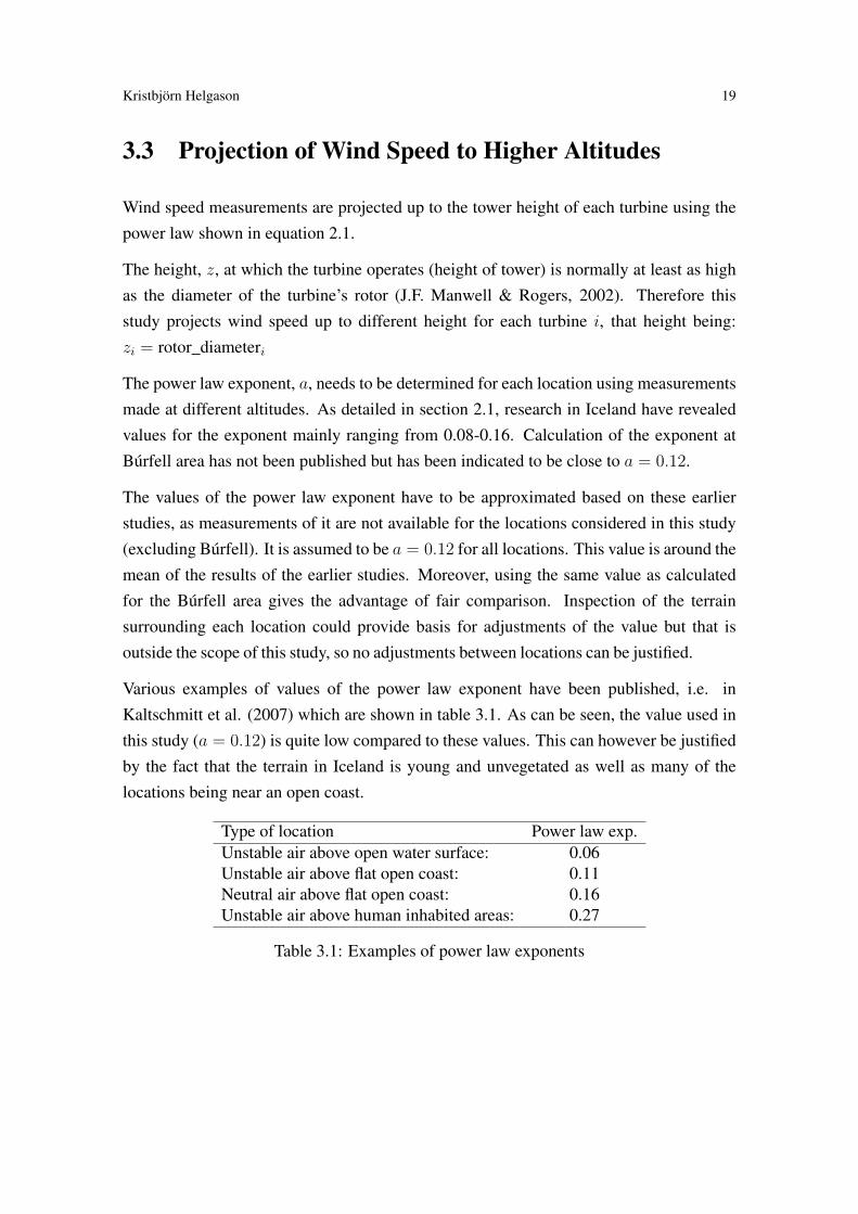
Various examples of values of the power law exponent have been published, i.e. inKaltschmitt et al. (2007) which are shown in table 3.1. As can be seen, the value used inthis study (a = 0.12) is quite low compared to these values. This can however be justifiedby the fact that the terrain in Iceland is young and unvegetated as well as many of thelocations being near an open coast.
Type of location Power law exp.Unstable air above open water surface: 0.06Unstable air above flat open coast: 0.11Neutral air above flat open coast: 0.16Unstable air above human inhabited areas: 0.27
Table 3.1: Examples of power law exponents
20 Selecting optimum location and type of wind turbines in Iceland
3.4 Simulation of Wind Speed and Power
A simulation of future wind speeds is conducted using the Weibull parameters for eachmonth at each location. Each simulated value is converted into simulated power outputby using the corresponding value on the power curve of each turbine. The method ofAntithetic variables is used to reduce number of iterations needed, as discussed in section2.3. The process of simulation is described in the following steps:
1. Generate a random number, U1 (uniform between 0 and 1) and also set U2 = 1−U1
2. Use Inverse Transform to get two simulated wind speed values,Xi = F (Ui, km, λm)
where F (x, k, λ) is the cumulative distribution Weibull function with the Weibullparameters,k and λ for month m.
3. Multiply Xi with (zj/10)0.12 (where z is the height of turbine j) and set Vi =
Xi · (zj/10)0.12 as a simulated value for wind at height zj
4. Look up the power output corresponding to wind value Vi, on the power curve ofturbine j and record it as Pi
5. Repeat steps 1−4, k-times
6. The mean of the power outputs of the k runs gives the expected power output inmonth m for turbine j, P =
∑ki=1 Pi /k
The number of simulation runs, k, is decided such that the standard deviation of expectedpower output, S, is less than 0.2% of the rated power of the turbine, with 95% certainty.Ross (2006) gives the following equation to decide on k, using 95% certainty level
1.96S√k
< d , for k > 100 (3.3)
where d is the acceptable value of the standard deviation of the estimator (measured inkW). For a 2MW turbine, d = 4 and using eq. 3.3, the number k can be decided.
One value of k is estimated to use for all the simulations. Using one 2MW turbine, one3MW turbine and one 1.25MW turbine, at a specific location for specific month gives arage of k’s. The resulting k’s are all in the range of 40,000-50,000 iterations.
Therefore k = 50,000 is used when simulating data for each month for each weatherstation.

Kristbjörn Helgason 21
3.5 Energy calculation
All energy and efficiency calculations in the study assume 100% availability of the tur-bine, i.e. no downtime due to maintenance or malfunction is estimated.
3.5.1 Energy output
Each wind turbine has its unique power curve which represents the efficiency of its opera-tion in various wind speeds. Appendix B shows the defining values for each of the turbinesconsidered. Those are: Cut-in speed, cut-off speed and power output of operation for thecertified wind speed range.
Since this study covers 47 different turbines for which only discrete power curve valuesare known, the energy output calculations are estimated using sums (equivalent to usingthe Riemann sum to estimate integrals). The wind speeds are generated by simulationbased on the calculated Weibull distribution of each month. Each generated value repre-sents wind speed over ten minute interval. The values on the power curve correspondingto each wind value are multiplied with the time interval of each wind value (1
6of an hour
to get a value in kWh). Those values are summed up to give an estimate of the averagetotal energy generated each month and year, respectively,
Emonthj =1
N
N∑i=1
Pwi· 1
6· 24 ·Dj (3.4)
Eyear =12∑j=1
Emonthj (3.5)
where wi is the ith simulated wind value, N is the total number of values simulated, Pwi
is the power curve value corresponding to the simulated wind and Dj is the number ofdays per month j.
This estimation of the average energy generated per year is calculated for each turbine ateach location. The outcome is used to measure the cost of energy for each setup, which iscomparable between different sizes, as is described in section 3.7.3.
22 Selecting optimum location and type of wind turbines in Iceland
3.5.2 Capacity factor
The capacity factor describes how well a wind turbine is utilizing the installed powerat a specific location by stating the ratio between the power actually produced and therated power of the turbine. In this study, it is used to give an indication of how welleach turbine matches a specific location. The formula for the capacity factor is shown inequation 2.8
3.6 Distance from weather stations to substations
The cost of connecting a certain wind location to the energy grid needs to be estimated bycalculating the distance from that location to the next substation of the energy grid.
All locations are provided in geographic longitude and latitude coordinates, in degrees.Distance between two points on a sphere is calculated by the great-circle distance
d = R · arccos(sinφ1 sinφ2 + cosφ1 cosφ2 cos |λ1 − λ2|) (3.6)
whereR is the radius of the earth at Iceland’s latitude, and φi, λi are latitude and longitudeat points i = 1, 2, respectively.
Earth’s radius at the equator is a = 6378.1 km and at the poles b = 6356.8 km (Moritz,2000). The latitude at the center of Iceland is approximately φ = 65N. Earth’s radius atthat latitude is calculated using ellipsoidal trigonometry
R =
√(a2 · cos(φ))2 + (b2 · sin(φ))2
(a · cos(φ))2 + (b · sin(φ))2= 6361 km (3.7)
At each location, the distance di is the distance to substation i. By finding min di ∀i, thedistance to the next substation is calculated for all locations. The calculated distances areshown in appendix C.

Kristbjörn Helgason 23
3.7 Cost analysis
3.7.1 Setup and operational costs
The cost of turbines are considered to be proportional to the swept rotor area as suggestedby the European Wind Energy Association in (Krohn et al., 2009) and (EWEA, 2009b).Price per rotor swept area is considered to be 460 e /m2 which is the latest publishedvalue and close to a long-term mean, as shown in figure 2.1.
Other cost estimations used by EWEA in its cost of energy calculations is adopted in thisstudy. These estimates are:
- Operation and maintenance (O&M) costs are assumed to be 1.45 ce /kWh as anaverage over the lifetime of the turbine
- The lifetime of the turbine is set at 20 years, in accordance with most technicaldesign criteria
- The discount rate is assumed to range from 5 to 10 % per annum. In the calculations,a discount rate of 7.5 % per annum is used
(EWEA, 2009b).
3.7.2 Connection cost
The cost per kilometer of 33kV connection line is estimated to be approximately 80, 000e /km,as discussed in section 2.3. This line suffices for transmission of the power produced inall cases of this study as it never exceeds 3.6MW (for any single turbine). This is likelyto rather be an overestimate than underestimate, specially for the smaller turbines.
Landsnet charges a fixed annual delivery fee of 4,317,536 ISK, approximately e 26,000(Landsnet, 2012b). This fee is added to the operation cost in the cost of energy calcula-tions.
Additionally, Landsnet charges for Ancillary Services and transmission losses per MWh.The current price is ce 0.44 per kWh (77.4 ISK), which is added to the O&M costs in thisstudy.
24 Selecting optimum location and type of wind turbines in Iceland
3.7.3 Cost of energy
The cost of energy (COE) is the total cost per kWh produced. It is calculated by dis-counting investment and O&M costs over the lifetime of the turbine and dividing it bythe annual electricity production. Thus, the COE is calculated as an average cost over theturbine’s lifetime .
J.F. Manwell and Rogers (2002) give the following equations for calculating COE whenonly cost is considered (not cash flow or any effect of selling price)
CRF =annual_payment
present_value= r/[1− (1 + r)−N ] (3.8)
NPVC = Pd + Pa · Y(
1
1 + r,N
)+ COM · Y
(1 + i
1 + r, L
)(3.9)
Y (k, l) =k − kl+1
1− k(3.10)
COE =NPVc · CRF
Annual_energy_production(3.11)
where:Pd = downpayment on system costs, estimated as 10%Pa = annual payment on system costs = (Cc − Pd) · CRFCRF = capital recovery factor, based on the loan interest rate, b, rather than rNPVC = net present value of cost factorsY = function to obtain the present value of a series of paymentsb = loan interest rate, estimated 7.5%, in accordance with current gov. bond marketr = discount rate, estimated 7.5% as suggested by EWEAi = inflation rate, 0%, no effect of inflation as constant prices are consideredL = lifetime of system, 20 years as suggested by EWEAN = period of loan, 20 years as the lifetime of the systemCc = capital cost of system, 460 e /m2 × rotor_area + 80000 e /km×djdj = distance from location j to nearest substationCOM = annual O&M cost, 1.45 ce /kWh+0.44 ce /kWh+26000 e
The cost of energy can be used to estimate whether a certain wind turbine setup is eco-nomically feasible. If COE is higher than the sales price of the electricity, the constructionis not feasible. Current sales price in Iceland, without transport, is 4.74 kr/kWh or around3 ce /kWh (OR.is / Prices / Rates, 2012).

Kristbjörn Helgason 25
Sensitivity analysis or certainty estimates are outside the scope of this study. The COEis meant to be an indication to compare the different setup and not a full scale feasibilitystudy. Nonetheless, two significant digits are used in the results, as they are justifiablewhen using the specific assumptions listed above.
3.7.4 Transmission losses
Loss in transmission is related to the distance of the transmission as well as characteristicsof the line. Losses are described by Ohm’s law as
Pl = IVd = I2R (3.12)
where Pl is the power lost, I is the current in the transmission line, Vd is the voltage dropover the distance and R is the resistance of the line (typical value is 0.15 Ω/km). Thecurrent is I = P/V where P is the power being transmitted and V the voltage of thepower.
In the case of the biggest turbine (3.6MW), average capacity factor of 50% and typicaldistance (15 km) the loss is, Pl = (1800kW/33kV )2·0.15Ω/km·15km = 6.7 kW, or only0.4% of the average 1800 kW power transmitted. This is well within other uncertaintyfactors such as O&M costs or cost of the connection line, and therefore the cost of loss intransmission is omitted in this study.
3.8 Limitations
This study does not cover all the complex factors needed to be evaluated when decidingon locations for wind turbines. A few of those not covered, are listed below as limita-tions.
3.8.1 Wind measurements and locations
The selection of locations considered in this study is limited to weather stations whichmay not be the optimum locations for wind turbines. Moreover, those measurements areall made at altitudes of around 10m. More extensive wind measurements are needed toget a more detailed view of prospective locations.

26 Selecting optimum location and type of wind turbines in Iceland
The effect of the terrain surface on wind speeds have only been studied for a few loca-tions in Iceland. In this study, that effect is approximated to be the same at all locationsconsidered and thus overly simplifying the effect. This simplification is made due to lackof information on the terrain at each location. This has effect on the magnitude of windwhen projected up to higher altitudes.
3.8.2 Turbine cost
The turbine market price is driven by individual quotes and a precise price for each turbineis hard to get without an actual bidding process. The prices used in this study are estimatedprices using data from the European Wind Energy Association (EWEA, 2009a). Pricesare assumed to be linearly related to the rotor diameter of the turbine. More precise pricesare needed for a study like this to be used as ground for decision making.
The cost of operation and maintenance, is also approximated to be linearly related topower produced, using averages published by EWEA. These costs are to some extentlocationally dependent and should therefore differ somewhat between locations and evencountries. Due to the lack of experience of wind power usage in Iceland, no more detaileddata is available.
3.8.3 Environmental issues
Environmental issues that should be addressed before permitting the setup of a commer-cial wind turbine include impacts on wildlife, habitat and other environmentally sensitivefactors. A special concern for the habitats is noise and visual pollution, as a large tur-bine can be around 100 meters high and emit sound exceeding 100dB in its proximity.A wind turbine might pose a serious threat to many species of birds and their breedingareas.
The evaluation of those factors are beyond the scope of this study. Nonetheless, they arecritical to further implementation of wind power in Iceland and need detailed research.The outcome of such research can affect heavily the process of locating of future windpower plants.

27
Chapter 4
Results
4.1 Wind Analysis and Simulation
To get a rough estimate of which locations could be feasible as a location for a windturbine, average annual wind speeds are compared. Figure 4.1 shows the top ten locationswith the highest annual mean wind speed. Bjarnarey has the highest annual mean windspeed over the period measured, 8.6 m/s in average.
1
2
3
4
5
6
7
89
10
Bjarnarey
Garðskagaviti
Rauðinúpur
Skagatá
Gufuskálar
Gjögurflugvöllur
Seley
BúrfellMiðdalsheiði
Fontur
8.6 m/s
8.4 m/s
8.3 m/s
7.4 m/s
7.4 m/s
7.1 m/s
7 m/s
7 m/s7 m/s
6.8 m/s
Figure 4.1: Top ten locations with the highest annual mean wind speed,ordered from 1 to 10
28 Selecting optimum location and type of wind turbines in Iceland
4
6
8
10
Bjarnarey
Garðskagaviti
Rauðinúpur
Skagatá
GufuskálarGjögurflugvöllur
Seley
Búrfell
MiðdalsheiðiFonturHafnarmelar
SkarðsfjöruvitiSiglunesSkrauthólar
Vattarnes
Þykkvibær
Hornbjargsviti
Straumsvík
KambanesDalatangi
Reykjavíkurflugvöllur
Mývatn
HvanneyriSámsstaðir
Flateyri
Month
Mea
nw
ind
spee
d[m
/s]
Feb Apr Jun Aug Oct Dec
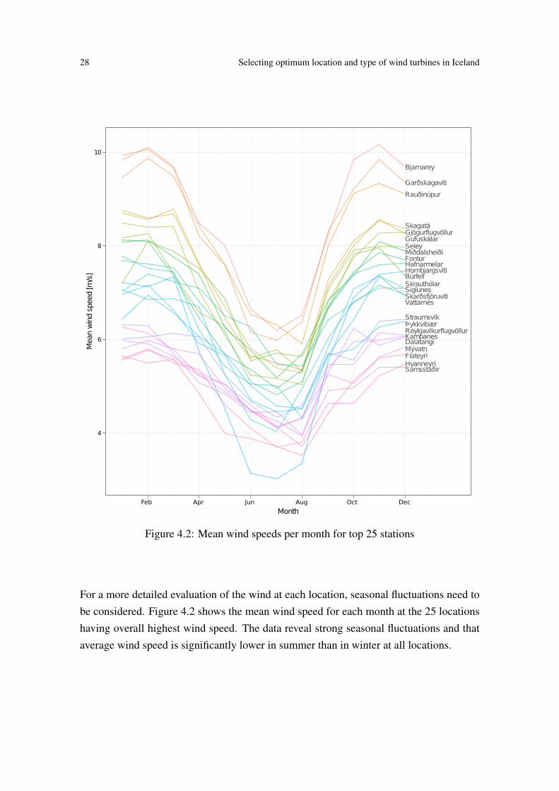
Figure 4.2: Mean wind speeds per month for top 25 stations
For a more detailed evaluation of the wind at each location, seasonal fluctuations need tobe considered. Figure 4.2 shows the mean wind speed for each month at the 25 locationshaving overall highest wind speed. The data reveal strong seasonal fluctuations and thataverage wind speed is significantly lower in summer than in winter at all locations.
Kristbjörn Helgason 29
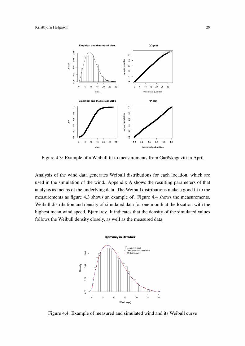
Figure 4.3: Example of a Weibull fit to measurements from Garðskagaviti in April
Analysis of the wind data generates Weibull distributions for each location, which areused in the simulation of the wind. Appendix A shows the resulting parameters of thatanalysis as means of the underlying data. The Weibull distributions make a good fit to themeasurements as figure 4.3 shows an example of. Figure 4.4 shows the measurements,Weibull distribution and density of simulated data for one month at the location with thehighest mean wind speed, Bjarnarey. It indicates that the density of the simulated valuesfollows the Weibull density closely, as well as the measured data.
Bjarnarey inOctober
Wind [m/s]
Density
0 5 10 15 20 25 30
0.00
0.02
0.04
0.06
l−_
MeasuredwindDensity of simulatedwindWeibull curve
ll
Figure 4.4: Example of measured and simulated wind and its Weibull curve
30 Selecting optimum location and type of wind turbines in Iceland
4.2 Annual Energy Output
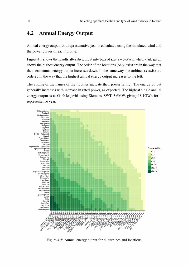
Annual energy output for a representative year is calculated using the simulated wind andthe power curves of each turbine.
Figure 4.5 shows the results after dividing it into bins of size 2−5 GWh, where dark greenshows the highest energy output. The order of the locations (on y-axis) are in the way thatthe mean annual energy output increases down. In the same way, the turbines (x-axis) areordered in the way that the highest annual energy output increases to the left.
The ending of the names of the turbines indicate their power rating. The energy outputgenerally increases with increase in rated power, as expected. The highest single annualenergy output is at Garðskagaviti using Siemens_SWT_3.6MW, giving 18.1GWh for arepresentative year.
GarðskagavitiRauðinúpur
BjarnareyGufuskálar
SkagatáSeley
BúrfellGjögurflugvöllur
FonturMiðdalsheiði
SkarðsfjöruvitiHafnarmelar
VattarnesSiglunes
ÞykkvibærStraumsvíkSkrauthólar
HornbjargsvitiReykjavíkurflugvöllur
KambanesDalatangi
MývatnHvanneyri
SámsstaðirFlateyri
BolungarvíkStraumnesvitiPatreksfjörður
KorpaEgilsstaðaflugvöllur
Végeirsstaðir í FnjóskadalÁsbyrgi
EskifjörðurÓlafsfjörður
SeyðisfjörðurHúsafell
Reykir í FnjóskadalSúðavík
TeigarhornÞingvellirReykjavík
SiglufjörðurÍsafjörðurKollaleira
BíldudalurNeskaupstaður
SkaftafellHallormsstaður
Siemen
s_SWT_
3.6MW
GE_3.6s
l_111
m_360
0kW
Enerco
n_E10
1_10
1m_3
000k
W
Leitw
ind_L
TW10
1m_3
MW
Vesta
s_V90
_3MW
Siemen
s_SWT_
101m
_2.3M
W
Clippe
r_C10
0_10
0m_2
500k
W
GE_2.5x
l_100
m_250
0kW
Clippe
r_C96
_96m
_250
0kW
Nordex
_N10
0_25
00kW
Enerco
n_E82
_82m
_300
0kW
Clippe
r_C93
_93m
_250
0kW
Nordex
_N90
_250
0kW
Siemen
s_SWT_
93m_2
.3MW
Clippe
r_C89
_89m
_250
0kW
Enerco
n_E82
_82m
_230
0kW
Vesta
s_V_9
0_Grid
Stream
er_2M
W
Enerco
n_E82
_E2_
82m_2
000k
W
Games
a_G90
_2.0M
W
Games
a_G87
_2.0M
W
Bonus
_82.4
m_2.3M
WGE_1
.6MW
Games
a_G83
_2.0M
W
Vesta
s_80
m_2MW
Enerco
n_E70
_71m
_230
0kW
Games
a_G80
_2.0M
W
Leitw
ind_L
TW80
_1.8M
W
Vesta
s_V82
_1.65
MW
AAER_A16
50_8
2m_1
650k
W
Leitw
ind_L
TW80
_1.5M
W
Leitw
ind_L
TW70
_2MW
AAER_A16
50_7
7m_1
650k
W
Leitw
ind_L
TW77
m_1.5M
W
Leitw
ind_L
TW70
_1.7M
W
Nordex
_S77
_150
0kW
GE_1.5s
l_77m
_150
0kW
Nordex
_S70
_150
0kW
Nordex
_N70
__1.5
MW
Nordex
_N60
__1.3
MW
Games
a_G58
_850
kW
Enerco
n_E53
_52.9
m_800
kW
Games
a_G52
_850
kW
Vesta
s_V52
_850
kW
Enerco
n_E48
_48m
_800
kW
Enerco
n_E44
_44m
_900
kW
Bonus
_MkIV
_44m
_600
kW
Enerco
n_E33
_33.4
m_330
kW
Energy [GWh](0,2](2,4](4,6](6,8](8,10](10,14](14,19]
Figure 4.5: Annual energy output for all turbines and locations
Kristbjörn Helgason 31
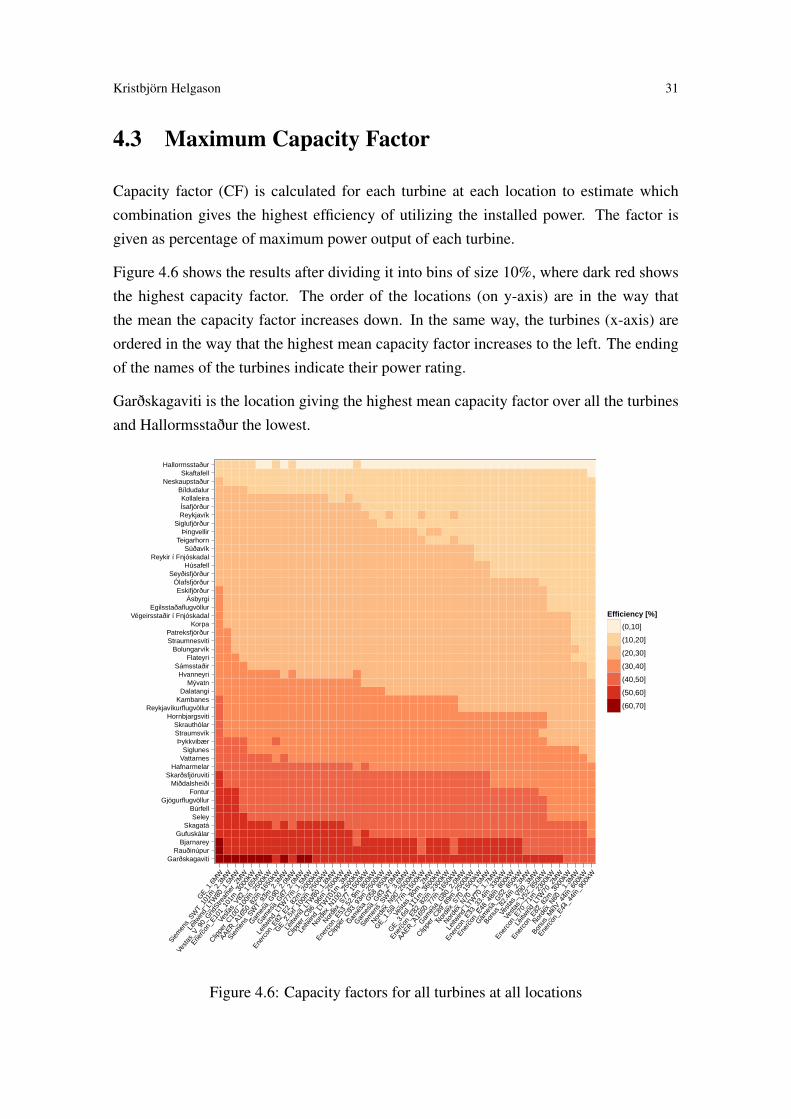
4.3 Maximum Capacity Factor
Capacity factor (CF) is calculated for each turbine at each location to estimate whichcombination gives the highest efficiency of utilizing the installed power. The factor isgiven as percentage of maximum power output of each turbine.
Figure 4.6 shows the results after dividing it into bins of size 10%, where dark red showsthe highest capacity factor. The order of the locations (on y-axis) are in the way thatthe mean the capacity factor increases down. In the same way, the turbines (x-axis) areordered in the way that the highest mean capacity factor increases to the left. The endingof the names of the turbines indicate their power rating.
Garðskagaviti is the location giving the highest mean capacity factor over all the turbinesand Hallormsstaður the lowest.
GarðskagavitiRauðinúpur
BjarnareyGufuskálar
SkagatáSeley
BúrfellGjögurflugvöllur
FonturMiðdalsheiði
SkarðsfjöruvitiHafnarmelar
VattarnesSiglunes
ÞykkvibærStraumsvíkSkrauthólar
HornbjargsvitiReykjavíkurflugvöllur
KambanesDalatangi
MývatnHvanneyri
SámsstaðirFlateyri
BolungarvíkStraumnesvitiPatreksfjörður
KorpaVégeirsstaðir í Fnjóskadal
EgilsstaðaflugvöllurÁsbyrgi
EskifjörðurÓlafsfjörður
SeyðisfjörðurHúsafell
Reykir í FnjóskadalSúðavík
TeigarhornÞingvellir
SiglufjörðurReykjavíkÍsafjörðurKollaleira
BíldudalurNeskaupstaður
SkaftafellHallormsstaður
GE_1
.6M
W
Siem
ens_
SWT_
101m
_2.3
MW
Leitw
ind_
LTW
80_1
.5M
W
Vest
as_V
_90_
Grid
Stream
er_2
MW
Enerc
on_E
101_
101m
_300
0kW
Vest
as_V
82_1
.65M
W
Clippe
r_C10
0_10
0m_2
500k
W
AAER_A16
50_8
2m_1
650k
W
Siem
ens_
SWT_
93m
_2.3
MW
Gam
esa_
G90
_2.0
MW
Gam
esa_
G87
_2.0
MW
Leitw
ind_
LTW
77m
_1.5
MW
Enerc
on_E
82_E
2_82
m_2
000k
W
GE_2
.5xl_
100m
_250
0kW
Leitw
ind_
LTW
80_1
.8M
W
Clippe
r_C96
_96m
_250
0kW
Leitw
ind_
LTW
101m
_3M
W
Norde
x_N10
0_25
00kW
Norde
x_S77
_150
0kW
Enerc
on_E
53_5
2.9m
_800
kW
Clippe
r_C93
_93m
_250
0kW
Gam
esa_
G58
_850
kW
Gam
esa_
G83
_2.0
MW
Siem
ens_
SWT_
3.6M
W
Norde
x_N90
_250
0kW
GE_1
.5sl_
77m
_150
0kW
Vest
as_8
0m_2
MW
GE_3
.6sl_
111m
_360
0kW
Enerc
on_E
82_8
2m_2
300k
W
AAER_A16
50_7
7m_1
650k
W
Gam
esa_
G80
_2.0
MW
Clippe
r_C89
_89m
_250
0kW
Norde
x_S70
_150
0kW
Norde
x_N70
__1.
5MW
Leitw
ind_
LTW
70_1
.7M
W
Enerc
on_E
33_3
3.4m
_330
kW
Enerc
on_E
48_4
8m_8
00kW
Gam
esa_
G52
_850
kW
Bonus
_82.
4m_2
.3M
W
Vest
as_V
90_3
MW
Vest
as_V
52_8
50kW
Enerc
on_E
70_7
1m_2
300k
W
Leitw
ind_
LTW
70_2
MW
Enerc
on_E
82_8
2m_3
000k
W
Norde
x_N60
__1.
3MW
Bonus
_MkI
V_44m
_600
kW
Enerc
on_E
44_4
4m_9
00kW
Efficiency [%]
(0,10]
(10,20]
(20,30]
(30,40]
(40,50]
(50,60]
(60,70]
Figure 4.6: Capacity factors for all turbines at all locations

32 Selecting optimum location and type of wind turbines in Iceland
0.35
0.40
0.45
0.50
0.55
0.60
0.65
GE_
1.6M
W
Siem
ens_
SWT_
101m
_2.3
MW
Leitw
ind_
LTW
80_1
.5M
W
Vest
as_V
_90_
Grid
Stre
amer
_2M
W
Vest
as_V
82_1
.65M
W
Ener
con_
E101
_101
m_3
000k
W
Clippe
r_C10
0_10
0m_2
500k
W
Siem
ens_
SWT_
93m
_2.3
MW
Leitw
ind_
LTW
77m
_1.5
MW
Gam
esa_
G87
_2.0
MW
Ener
con_
E82_
E2_8
2m_2
000k
W
GE_
2.5x
l_10
0m_2
500k
W
Leitw
ind_
LTW
80_1
.8M
W
Clippe
r_C96
_96m
_250
0kW
Norde
x_S7
7_15
00kW
Leitw
ind_
LTW
101m
_3M
W
Ener
con_
E53_
52.9
m_8
00kW
AAER
_A16
50_8
2m_1
650k
W
Gam
esa_
G90
_2.0
MW
Clippe
r_C93
_93m
_250
0kW
Gam
esa_
G83
_2.0
MW
GE_
3.6s
l_11
1m_3
600k
W
Norde
x_N90
_250
0kW
Vest
as_8
0m_2
MW
Siem
ens_
SWT_
3.6M
W
Ener
con_
E82_
82m
_230
0kW
Gam
esa_
G58
_850
kW
Norde
x_N70
__1.
5MW
Norde
x_S7
0_15
00kW
Norde
x_N10
0_25
00kW
Gam
esa_
G80
_2.0
MW
Clippe
r_C89
_89m
_250
0kW
GE_
1.5s
l_77
m_1
500k
W
Leitw
ind_
LTW
70_1
.7M
W
Ener
con_
E33_
33.4
m_3
30kW
Gam
esa_
G52
_850
kW
AAER
_A16
50_7
7m_1
650k
W
Bonu
s_82
.4m
_2.3
MW
Ener
con_
E48_
48m
_800
kW
Vest
as_V
90_3
MW
Vest
as_V
52_8
50kW
Ener
con_
E70_
71m
_230
0kW
Leitw
ind_
LTW
70_2
MW
Ener
con_
E82_
82m
_300
0kW
Norde
x_N60
__1.
3MW
Bonu
s_M
kIV_
44m
_600
kW
Ener
con_
E44_
44m
_900
kW
CF
Rotor size [m]
45
70
95
Location
Garðskagaviti
Rauðinúpur
Bjarnarey
Gufuskálar
Skagatá
Seley
Búrfell
Gjögurflugvöllur
Fontur
Miðdalsheiði
Figure 4.7: Capacity factors of all turbines for the ten locationsthat have the highest capacity factors
Figure 4.7 shows the top ten locations that have the highest mean capacity factor. In thisfigure, a more precise value of the capacity factor of each turbine can be visualized.
The color of the dots indicates the location, and the size of the dots indicate the rotordiameter of each turbine. It can be seen that the efficiency roughly decreases with de-creasing rotor size although some exceptions therefrom are visible. The most effectiveturbines tend to have relatively large rotor size compared to its rated power (rated poweris shown in each turbine’s name).
As figures 4.6 and 4.7 show, the turbine GE_1.6MW has the highest efficiency at alllocations. This turbine is unusual in the way that, in spite of having a large rotor diameterof 101 meters, it is rated only 1.6MW. This rotor diameter is typical for a turbine ratedaround 2.5-3.0MW. Therefore, this turbine gives high efficiency but will have low poweroutput compared to its setup cost. For this reason, this turbine is omitted in the nextcomparison, where locations having top ten capacity factors are mapped.

Kristbjörn Helgason 33
Figure 4.8: Top ten locations with the highest capacity factor,ordered from 1 to 10
Figure 4.8 shows a map where the locations with the highest capacity factors (exclud-ing the one that GE_1.6MW gives) are listed and ordered from one to ten, one be-ing the highest. At all locations, the turbine which gives the highest capacity factor isSiemens_SWT_101m_2.3MW, which also has a very high rotor diameter (101m), but israted 2.3MW.
A comparison between figures 4.8 and 4.1, where highest annual mean wind speed isordered, shows that the same top ten locations are selected but the order differs somewhat.The main reason is different wind profiles at the locations and it emphasizes that averagewind speed does not reveal all the potentials of a location for a wind turbine.
Generally, a capacity factor above 40% is regarded very good for wind turbine location.In that comparison, all ten locations listed in figure 4.8, have a very high capacity factor.Around half of all the locations can be regarded as good for wind turbine location in thissense.

34 Selecting optimum location and type of wind turbines in Iceland
4.4 Minimum Cost of Energy
The largest cost factor is in most cases the turbine cost. The exact cost of each turbineis not known but estimated as shown in section 3.7.1. However, if energy needs to betransmitted long distance from turbine to grid, the connection cost becomes a big factoras well. Appendix C shows the measured distances from each location to nearest gridsubstation.
Cost of energy (COE), measured in cent Euros per kWh (ce /kWh) is calculated dividingthe annual payment of the discounted total cost estimated for each turbine with the annualenergy output (shown previously in figure 4.5).
Figure 4.9 shows the cost of energy after dividing it into bins, where beige shows thelowest COE and dark blue the highest. The locations and turbines are ordered in such away that the combinations having the lowest COE are in the lower left corner.
Garðskagaviti is the location giving the lowest mean cost of energy over all the turbinesand Skaftafell gives the highest. The turbine that gives the lowest mean COE over all theturbines is Enercon_E101_101m_3000kW.
By looking at the locations on the y-axis of figure 4.9 it can be seen that the order differsa lot from the order in figure 4.6, where capacity factors are presented. This means thatthe turbine that have the highest capacity factors are not the one giving the lowest COE.The reason is that large rotor turbines generally have high capacity factor but as cost isrelated to rotor size, the capital cost is negatively affected by the large rotor.
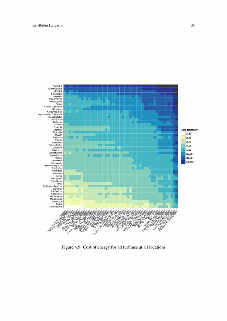
Kristbjörn Helgason 35
GarðskagavitiBúrfell
GufuskálarMiðdalsheiðiHafnarmelarStraumsvíkRauðinúpurBjarnarey
ReykjavíkurflugvöllurSeley
SkrauthólarBolungarvík
KorpaVattarnesÞykkvibærEskifjörður
EgilsstaðaflugvöllurSámsstaðirHvanneyriFlateyri
SeyðisfjörðurSkarðsfjöruviti
TeigarhornDalatangi
PatreksfjörðurKambanes
ÁsbyrgiÍsafjörðurMývatn
ReykjavíkSiglunesSkagatáSúðavíkKollaleira
ÓlafsfjörðurNeskaupstaður
Végeirsstaðir í FnjóskadalGjögurflugvöllur
BíldudalurReykir í Fnjóskadal
FonturHornbjargsvitiStraumnesviti
ÞingvellirSiglufjörður
HúsafellHallormsstaður
Skaftafell
Enercon_E101_101m_3000kW
Enercon_E82_82m_3000kW
Siemens_SW
T_3.6MW
Leitwind_LTW101m_3MW
Vestas_V90_3MW
GE_3.6sl_111m_3600kW
Enercon_E82_82m_2300kW
Enercon_E70_71m_2300kW
Nordex_N90_2500kW
Enercon_E82_E2_82m_2000kW
Clipper_C96_96m_2500kW
Clipper_C89_89m_2500kW
Clipper_C93_93m_2500kW
Siemens_SW
T_93m_2.3MW
Siemens_SW
T_101m_2.3MW
Clipper_C100_100m_2500kW
Bonus_82.4m_2.3MW
Nordex_N100_2500kW
GE_2.5xl_100m_2500kW
Vestas_80m_2MW
Vestas_V_90_GridStreamer_2MW
Gamesa_G87_2.0MW
Gamesa_G80_2.0MW
Leitwind_LTW70_2MW
Gamesa_G83_2.0MW
Leitwind_LTW80_1.8MW
Gamesa_G90_2.0MW
Leitwind_LTW70_1.7MW
AAER_A1650_82m_1650kW
Leitwind_LTW80_1.5MW
Vestas_V82_1.65MW
AAER_A1650_77m_1650kW
Leitwind_LTW77m_1.5MW
Nordex_S70_1500kW
Nordex_N70__1.5MW
Nordex_S77_1500kW
GE_1.5sl_77m_1500kW
GE_1.6MW
Nordex_N60__1.3MW
Enercon_E53_52.9m_800kW
Enercon_E48_48m_800kW
Gamesa_G58_850kW
Gamesa_G52_850kW
Enercon_E44_44m_900kW
Vestas_V52_850kW
Bonus_MkIV_44m_600kW
Enercon_E33_33.4m_330kW
COE [centEUR]
(4,5]
(5,6]
(6,7]
(7,9]
(9,12]
(12,15]
(15,25]
(25,50]
Figure 4.9: Cost of energy for all turbines at all locations
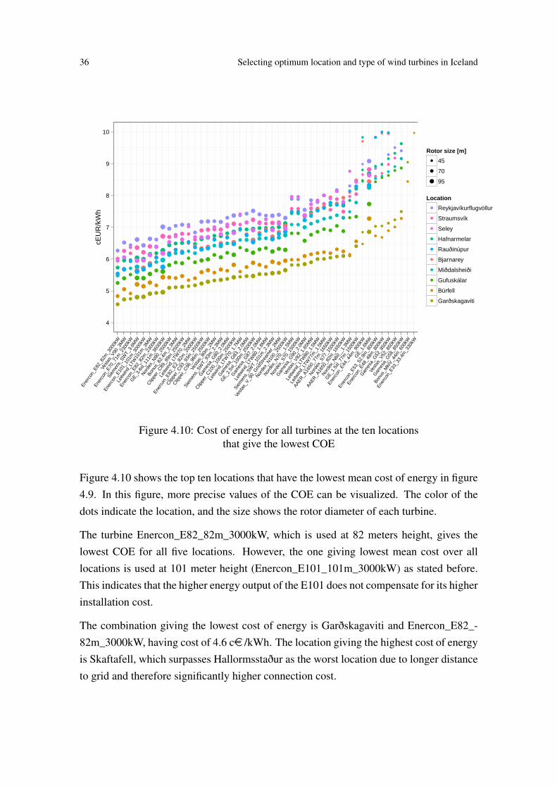
36 Selecting optimum location and type of wind turbines in Iceland
4
5
6
7
8
9
10
Ener
con_
E82_
82m
_300
0kW
Vest
as_V
90_3
MW
Ener
con_
E70_
71m
_230
0kW
Siem
ens_
SWT_
3.6M
W
Ener
con_
E101
_101
m_3
000k
W
Leitw
ind_
LTW
101m
_3M
W
Ener
con_
E82_
82m
_230
0kW
GE_
3.6s
l_11
1m_3
600k
W
Norde
x_N90
_250
0kW
Bonu
s_82
.4m
_2.3
MW
Clippe
r_C89
_89m
_250
0kW
Leitw
ind_
LTW
70_2
MW
Ener
con_
E82_
E2_8
2m_2
000k
W
Clippe
r_C93
_93m
_250
0kW
Clippe
r_C96
_96m
_250
0kW
Vest
as_8
0m_2
MW
Siem
ens_
SWT_
93m
_2.3
MW
Gam
esa_
G80
_2.0
MW
Clippe
r_C10
0_10
0m_2
500k
W
Leitw
ind_
LTW
70_1
.7M
W
Gam
esa_
G83
_2.0
MW
GE_
2.5x
l_10
0m_2
500k
W
Gam
esa_
G87
_2.0
MW
Leitw
ind_
LTW
80_1
.8M
W
Siem
ens_
SWT_
101m
_2.3
MW
Vest
as_V
_90_
Grid
Stre
amer
_2M
W
Norde
x_N10
0_25
00kW
Norde
x_N70
__1.
5MW
Norde
x_S7
0_15
00kW
Gam
esa_
G90
_2.0
MW
Vest
as_V
82_1
.65M
W
Leitw
ind_
LTW
80_1
.5M
W
Leitw
ind_
LTW
77m
_1.5
MW
AAER
_A16
50_7
7m_1
650k
W
Norde
x_S7
7_15
00kW
AAER
_A16
50_8
2m_1
650k
W
Norde
x_N60
__1.
3MW
GE_
1.5s
l_77
m_1
500k
W
Ener
con_
E44_
44m
_900
kWG
E_1.
6MW
Ener
con_
E53_
52.9
m_8
00kW
Ener
con_
E48_
48m
_800
kW
Gam
esa_
G52
_850
kW
Vest
as_V
52_8
50kW
Gam
esa_
G58
_850
kW
Bonu
s_M
kIV_
44m
_600
kW
Ener
con_
E33_
33.4
m_3
30kW
cEU
R/k
Wh
Rotor size [m]
45
70
95
Location
Reykjavíkurflugvöllur
Straumsvík
Seley
Hafnarmelar
Rauðinúpur
Bjarnarey
Miðdalsheiði
Gufuskálar
Búrfell
Garðskagaviti
Figure 4.10: Cost of energy for all turbines at the ten locationsthat give the lowest COE
Figure 4.10 shows the top ten locations that have the lowest mean cost of energy in figure4.9. In this figure, more precise values of the COE can be visualized. The color of thedots indicate the location, and the size shows the rotor diameter of each turbine.
The turbine Enercon_E82_82m_3000kW, which is used at 82 meters height, gives thelowest COE for all five locations. However, the one giving lowest mean cost over alllocations is used at 101 meter height (Enercon_E101_101m_3000kW) as stated before.This indicates that the higher energy output of the E101 does not compensate for its higherinstallation cost.
The combination giving the lowest cost of energy is Garðskagaviti and Enercon_E82_-82m_3000kW, having cost of 4.6 ce /kWh. The location giving the highest cost of energyis Skaftafell, which surpasses Hallormsstaður as the worst location due to longer distanceto grid and therefore significantly higher connection cost.
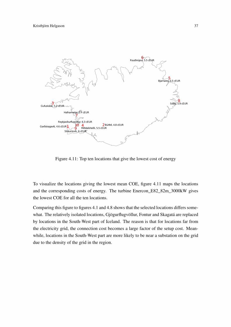
Kristbjörn Helgason 37
Figure 4.11: Top ten locations that give the lowest cost of energy
To visualize the locations giving the lowest mean COE, figure 4.11 maps the locationsand the corresponding costs of energy. The turbine Enercon_E82_82m_3000kW givesthe lowest COE for all the ten locations.
Comparing this figure to figures 4.1 and 4.8 shows that the selected locations differs some-what. The relatively isolated locations, Gjögurflugvöllur, Fontur and Skagatá are replacedby locations in the South-West part of Iceland. The reason is that for locations far fromthe electricity grid, the connection cost becomes a large factor of the setup cost. Mean-while, locations in the South-West part are more likely to be near a substation on the griddue to the density of the grid in the region.
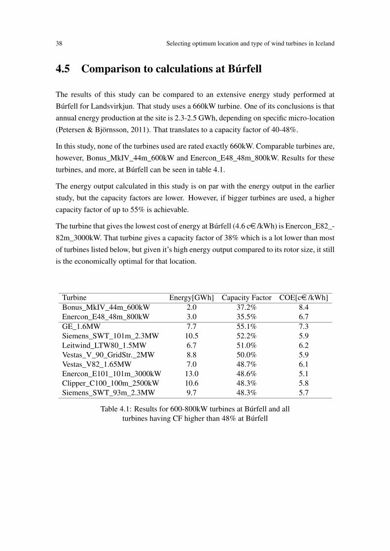
38 Selecting optimum location and type of wind turbines in Iceland
4.5 Comparison to calculations at Búrfell
The results of this study can be compared to an extensive energy study performed atBúrfell for Landsvirkjun. That study uses a 660kW turbine. One of its conclusions is thatannual energy production at the site is 2.3-2.5 GWh, depending on specific micro-location(Petersen & Björnsson, 2011). That translates to a capacity factor of 40-48%.
In this study, none of the turbines used are rated exactly 660kW. Comparable turbines are,however, Bonus_MkIV_44m_600kW and Enercon_E48_48m_800kW. Results for theseturbines, and more, at Búrfell can be seen in table 4.1.
The energy output calculated in this study is on par with the energy output in the earlierstudy, but the capacity factors are lower. However, if bigger turbines are used, a highercapacity factor of up to 55% is achievable.
The turbine that gives the lowest cost of energy at Búrfell (4.6 ce /kWh) is Enercon_E82_-82m_3000kW. That turbine gives a capacity factor of 38% which is a lot lower than mostof turbines listed below, but given it’s high energy output compared to its rotor size, it stillis the economically optimal for that location.
Turbine Energy[GWh] Capacity Factor COE[ce /kWh]Bonus_MkIV_44m_600kW 2.0 37.2% 8.4Enercon_E48_48m_800kW 3.0 35.5% 6.7GE_1.6MW 7.7 55.1% 7.3Siemens_SWT_101m_2.3MW 10.5 52.2% 5.9Leitwind_LTW80_1.5MW 6.7 51.0% 6.2Vestas_V_90_GridStr._2MW 8.8 50.0% 5.9Vestas_V82_1.65MW 7.0 48.7% 6.1Enercon_E101_101m_3000kW 13.0 48.6% 5.1Clipper_C100_100m_2500kW 10.6 48.3% 5.8Siemens_SWT_93m_2.3MW 9.7 48.3% 5.7
Table 4.1: Results for 600-800kW turbines at Búrfell and allturbines having CF higher than 48% at Búrfell

39
Chapter 5
Conclusions
5.1 Conclusions
Three measures of the performance of a combination of location and wind turbine typehave been calculated, annual energy output, capacity factor (CF) and cost of energy(COE). A total of 2256 combinations of locations and turbines have been calculated andcompared.
The results show that Garðskagaviti is the optimal location for a wind turbine in Iceland(out of the locations considerde), both in views of the highest efficiency in regards ofcapacity factor and when viewing the lowest cost of energy, 4.6 cEUR/kWh. This cost ishowever significantly higher than the sales price of electricity in Iceland which is around3 ce /kWh, excluding transport.
Different turbines are selected as optimal, depending on if the objective is to maximize thecapacity factor or minimize the cost of energy. For locations with high mean wind speedsthe turbine Enercon_E82_82m_3000kW is the one giving the lowest cost of energy butfor locations with lower wind speeds, the bigger Enercon_E101_101m_3000kW is theturbine giving the lowest cost. It is interesting that these are mainly the same turbines,differing only in rotor size.
As turbine cost is estimated to be linearly related to the rotor size, the Enercon_E82_82m-_3000kW has the advantage of having a high power rating but only medium sized rotor.That kind of turbine shows to be very cost efficient at locations where wind is strong andshould be considered for that kind of installations.
The turbines with the lowest power rating generally give the highest cost of energy asannual cost are high relative to the low energy generation.
40 Selecting optimum location and type of wind turbines in Iceland
Distance of locations to the electricity grid play a significant role when looking at theCOE. This can be seen at a location such as Bjarnarey which has the highest annual meanwind, the third highest overall capacity factor but drops to eighth in the minimum COEdue to high connection costs. The same applies to Rauðinúpur which also seems likea favorable location, if not for the high connection cost. These location could howeverbe favorable for small scale power generation to be utilized in the proximity of the tur-bine.
The cost of energy is in all cases significantly higher than the current sales price of energyin Iceland, where lowest calculated COE is 4,6 ce /kWh while sales price is around 3ce /kWh. Therefore, the production of wind power for direct sale is not currently feasi-ble.
If plans of a submarine cable to Europe follow through, the scenario could be totally dif-ferent as was pointed out by Sigurjónsson (2009). The sales price of electricity in theEuropean Union exceeds 10 ce /kWh in most countries, so wind power generation in Ice-land could become feasible, depending on cost of transport and transmission losses.
The comparison to other calculations at Búrfell confirms the high capacity factors fromthat studies. Furthermore, the COE calculations show that Búrfell has the second lowestCOE and thus makes the location even more feasible for wind generation. Therefore, thechoice of Landsvirkjun to construct their first wind turbine at the Búrfell area seems veryreasonable.
5.2 Summary of contribution
Wind measurements for 48 locations around Iceland have been statistically analyzed foreach month of the year. Such detailed analysis of these locations has not been publishedearlier. The resulting Weibull parameters are presented in Appendix A. Using thoseparameters, future wind is simulated.
The simulated wind is used along with the power curve of 47 different wind turbine types,which were collected in this study. This gives energy output for each turbine at eachlocation.
To compare the 2256 different combinations of location and type, the Capacity Factorand Cost of Energy have been calculated for each one and ordered accordingly. Thetwo performance measures give different perspectives on the quality of each location andturbine type. The former does not incorporate the cost of different turbines or the cost of
Kristbjörn Helgason 41
utilizing each location. The latter one includes the estimated cost of turbine as well as thedifferent costs of setting up turbines at each location. This calculations could be extendedfurther as more information is gathered through research.
Capacity factors for a few turbines have earlier been studied in Iceland, in most casesbased on annual or semi-annual mean wind speeds while this study bases the calculationson monthly analyzed Weibull data.
The Cost of Energy calculations result in cost per kWh for each turbine at each location.Building on these estimates, one can get a rough idea whether a particular turbine at acertain location is feasible or not. None of the combinations studied deliver energy at afeasible cost for the current Icelandic market, as production costs exceed the sale price ofenergy in all cases, given the assumptions used in the cost analysis.
5.3 Future Research
For successfully integrating wind power into the Icelandic energy market, the governmentneeds to make a master plan for the utilization of wind power resources such as has beendone for hydro and geothermal energy resources. The plan could detail e.g. a plan onwhat the share of wind power should ultimately become, what areas should be protectedfrom wind power plants and what areas are suitable for wind power extraction.
Following such a plan, the locations for wind power plants could be optimized usingrelevant constraints. Such a research could implement the use of mixed integer linearprogramming which is known to be suitable for optimally locating different sources.
Before an implementation of a master plan is possible, more detailed wind profile mea-surements are needed, making measurements at different altitudes. The construction ofa wind atlas for Iceland is in the makings, which is a huge contribution to this field ofresearch.
The experimental construction of a wind turbine in the Búrfell area will give valuableinformation on the feasibility of wind power in Iceland. Operation and maintenance costneed to be studied along with availability percentage of such a large turbine in the harshand windy Icelandic nature.
The environmental effects of wind turbine construction in Iceland need to be carefullyresearched for successful implementation of wind power in Iceland. In particular, theamount of noise and visual pollution as well as the possible negative impact on birds andwildlife need to be considered.

42
43
References
Abul’Wafa, A. R. (2011, April). Matching wind turbine generators with wind regime inEgypt. Electric Power Systems Research, 81(4), 894–898.
Arason Þórður. (1998). Mat á vindi á fyrirhuguðum brúm í Reykjavík. Veðurstofa Ís-
lands(VÍ-G98017-TA01).Awea - wind energy faq. (n.d.). Retrieved 30.4.2012, from archive.awea.org/faq/basicwr.
htmlBlöndal, J., Birgisson, T., Björnsson, H., Jónasson, K., & Petersen, G. N. (2011, De-
cember). Vindhraðamælingar og sambreytni vinds (Report No. VÍ 2011-014).Veðurstofa Íslands.
Blöndal, Ó. G. (2011). Wind Energy - a Realistic Option in Iceland? Re-trieved 30.4.2012, from http://www.landsvirkjun.com/media/news/Wind-Energy.-A-Realistic-Option-in-Iceland.pdf
Bloomberg. (n.d.). Bloomberg new energy finance. Retrieved 10.4.2012, from http://www.bnef.com/Insight/2050
Celik, A. N. (2003). Weibull representative compressed wind speed data for energyand performance calculations of wind energy systems. Energy Conversion and
Management, 44(19), 3057 - 3072.Celik, A. N. (2004). A statistical analysis of wind power density based on the Weibull
and Rayleigh models at the southern region of Turkey. Renewable Energy, 29(4),593 - 604.
Chang, T., & Tu, Y. (2007). Evaluation of Monthly Capacity Factor of WECS UsingChronological and Probabilistic Wind Speed Data: A Case Study of Taiwan. Re-
newable Energy, 32(12), 1999-2010.EWEA. (2009a). Wind Energy-The Facts, Volume 2, Costs & Prices. Available from
http://www.ewea.orgEWEA. (2009b). Wind Energy-The Facts, Volume 3, The Economics of Wind Power.
Available from http://www.ewea.orgIcelandic Meteorological Office. (n.d.). Retrieved 30.4.2012, from www.vedur.is
44 Selecting optimum location and type of wind turbines in Iceland
J.F. Manwell, J. M., & Rogers, A. (2002). Wind Energy Explained - Theory, Design and
Application. John Wiley and Sons Ltd.Kaltschmitt, M., Streicher, W., & Wiese, A. (2007). Renewable Energy: Technology,
Economics, and Environment. Springer.Keyhani, A., Ghasemi-Varnamkhasti, M., Khanali, M., & Abbaszadeh, R. (2010). An
assessment of wind energy potential as a power generation source in the capital ofIran, Tehran. Energy, 35(1), 188–201.
Kleywegt, A. J., Shapiro, A., & Homem-de-Mello, T. (2002). The Sample AverageApproximation Method for Stochastic Discrete Optimization. SIAM Journal on
Optimization, 12(2), 479.Krohn, S., Morthorst, P.-E., & Awerbuch, S. (2009, Mar). The economics of wind energy.
Landsnet. (2011). Landsnet Annual Report 2010. Published online. Available fromhttp://landsnet.is/landsnet/upplysingatorg/skyrslur/
Landsnet. (2012a). Kerfisáætlun Landsnets 2012. Published online. Available fromhttp://landsnet.is/landsnet/upplysingatorg/skyrslur/
Landsnet. (2012b). Tariff for the Transmission of Electricity and Ancillary Services. Pub-lished online. Available from http://landsnet.is/landsnet/upplysingatorg/skyrslur/
Landsnet | Kostnaður. (n.d.). Retrieved 15.5.2012, from http://www.landsnet.is/linurogstrengir/kostnadur/
Landsvirkjun. (2012). Landsvirkjun Annual Report 2011. Published online. Availablefrom http://www.landsvirkjun.com/about-us/reports/
Lun, I. Y., & Lam, J. C. (2000). A study of Weibull parameters using long-term windobservations. Renewable Energy, 20(2), 145 - 153.
Moritz, H. (2000, 3). Geodetic Reference System 1980. Journal of Geodesy, 74, 128-162.Mortensen, N. G., & Laboratory, R. N. (2007). Getting started with WAsP 9. Risø
National Laboratory.Nefnd um sjálfbært orkusamfélag í Grímsey. (2003). Sjálfbært orkukerfi í Grímsey (Tech.
Rep.). Iðnaðarráðuneytið.OR.is / Prices / Rates. (2012). Retrieved 15.5.2012, from http://www.or.is/English/
Services/PricesRates/Orkuspárnefnd. (2011, October). Raforkuspá 2011-2050 (Tech. Rep. No. OS-2011/07).
Orkustofnun.Papoulis, A. (2002). Probability, random variables and stochastic processes (4th ed.).
Mcgraw Hill Higher Education.Petersen, G. N., & Björnsson, H. (2011, November). Veðurmælingar
og vindorkuútreikningar fyrir Búrfellssvæðið (Tech. Rep. No. LV-2011-104).Landsvirkjun.
Kristbjörn Helgason 45
Rosin, P., & Rammler, E. (1933). The Laws Governing the Fineness of Powdered Coal.Journal of the Institute of Fuel(7), 29–36.
Ross, S. M. (2006). Simulation (4th ed.). Elsevier Academic Press.Rubinstein, R., & Melamed, B. (1998). Modern simulation and modeling (Vol. 7). Wiley
New York.Schlichting, H. (1968). Boundary layer theory. 6th edition. McGraw-Hill, New York.Sherlock, R. (1951). Analyzing winds for frequency and duration. Meteorological Mono-
graphs, 4, 72–79.Sigurjónsson, K. (2009, April). Virkjun vindorku og sjávarorku á Íslandi.
Sigurðsson, F. H., Hjartarson, H., Antonsson, T. K., & Arason Þórður. (1999). Wind Ob-
servations at Eyri and Leirur in Reyðarfjörður (No. VÍ-G99015-TA03). VeðurstofaÍslands.
Valenzuela, J., & Mazumdar, M. (2000). Statistical analysis of electric power productioncosts. IIE Transactions, 32(12), 1139–1148.
The WindPower Program. (n.d.). Retrieved 2012-04-22, from http://www.wind-power-program.com/
Yeh, T., & Wang, L. (2008, June). A Study on Generator Capacity for Wind TurbinesUnder Various Tower Heights and Rated Wind Speeds Using Weibull Distribution.IEEE Transactions on Energy Conversion, 23(2), 592–602.

46
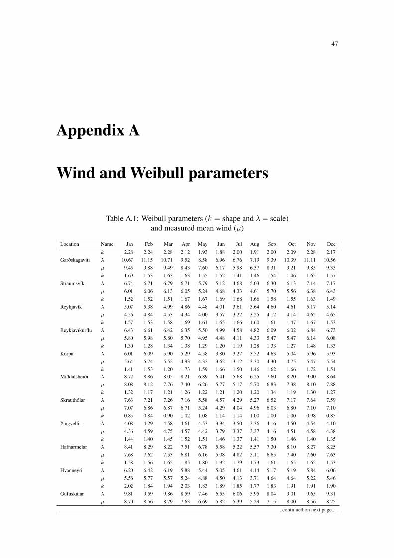
47
Appendix A
Wind and Weibull parameters
Table A.1: Weibull parameters (k = shape and λ = scale)and measured mean wind (µ)
Location Name Jan Feb Mar Apr May Jun Jul Aug Sep Oct Nov Dec
Garðskagavitik 2.28 2.24 2.28 2.12 1.93 1.88 2.00 1.91 2.00 2.09 2.28 2.17λ 10.67 11.15 10.71 9.52 8.58 6.96 6.76 7.19 9.39 10.39 11.11 10.56µ 9.45 9.88 9.49 8.43 7.60 6.17 5.98 6.37 8.31 9.21 9.85 9.35
Straumsvíkk 1.69 1.53 1.63 1.63 1.55 1.52 1.41 1.46 1.54 1.46 1.65 1.57λ 6.74 6.71 6.79 6.71 5.79 5.12 4.68 5.03 6.30 6.13 7.14 7.17µ 6.01 6.06 6.13 6.05 5.24 4.68 4.33 4.61 5.70 5.56 6.38 6.43
Reykjavíkk 1.52 1.52 1.51 1.67 1.67 1.69 1.68 1.66 1.58 1.55 1.63 1.49λ 5.07 5.38 4.99 4.86 4.48 4.01 3.61 3.64 4.60 4.61 5.17 5.14µ 4.56 4.84 4.53 4.34 4.00 3.57 3.22 3.25 4.12 4.14 4.62 4.65
Reykjavíkurfluk 1.57 1.53 1.58 1.69 1.61 1.65 1.66 1.60 1.61 1.47 1.67 1.53λ 6.43 6.61 6.42 6.35 5.50 4.99 4.58 4.82 6.09 6.02 6.84 6.73µ 5.80 5.98 5.80 5.70 4.95 4.48 4.11 4.33 5.47 5.47 6.14 6.08
Korpak 1.30 1.28 1.34 1.38 1.29 1.20 1.19 1.28 1.33 1.27 1.48 1.33λ 6.01 6.09 5.90 5.29 4.58 3.80 3.27 3.52 4.63 5.04 5.96 5.93µ 5.64 5.74 5.52 4.93 4.32 3.62 3.12 3.30 4.30 4.75 5.47 5.54
Miðdalsheiðik 1.41 1.53 1.20 1.73 1.59 1.66 1.50 1.46 1.62 1.66 1.72 1.51λ 8.72 8.86 8.05 8.21 6.89 6.41 5.68 6.25 7.60 8.20 9.00 8.64µ 8.08 8.12 7.76 7.40 6.26 5.77 5.17 5.70 6.83 7.38 8.10 7.88
Skrauthólark 1.32 1.17 1.21 1.26 1.22 1.21 1.20 1.20 1.34 1.19 1.30 1.27λ 7.63 7.21 7.26 7.16 5.58 4.57 4.29 5.27 6.52 7.17 7.64 7.59µ 7.07 6.86 6.87 6.71 5.24 4.29 4.04 4.96 6.03 6.80 7.10 7.10
Þingvellirk 0.85 0.84 0.90 1.02 1.08 1.14 1.14 1.00 1.00 1.00 0.98 0.85λ 4.08 4.29 4.58 4.61 4.53 3.94 3.50 3.36 4.16 4.50 4.54 4.10µ 4.36 4.59 4.75 4.57 4.42 3.79 3.37 3.37 4.16 4.51 4.58 4.38
Hafnarmelark 1.44 1.40 1.45 1.52 1.51 1.46 1.37 1.41 1.50 1.46 1.40 1.35λ 8.41 8.29 8.22 7.51 6.78 5.58 5.22 5.57 7.30 8.10 8.27 8.25µ 7.68 7.62 7.53 6.81 6.16 5.08 4.82 5.11 6.65 7.40 7.60 7.63
Hvanneyrik 1.58 1.56 1.62 1.85 1.80 1.92 1.79 1.73 1.61 1.65 1.62 1.53λ 6.20 6.42 6.19 5.88 5.44 5.05 4.61 4.14 5.17 5.19 5.84 6.06µ 5.56 5.77 5.57 5.24 4.88 4.50 4.13 3.71 4.64 4.64 5.22 5.46
Gufuskálark 2.02 1.84 1.94 2.03 1.83 1.89 1.85 1.77 1.83 1.91 1.91 1.90λ 9.81 9.59 9.86 8.59 7.46 6.55 6.06 5.95 8.04 9.01 9.65 9.31µ 8.70 8.56 8.79 7.63 6.69 5.82 5.39 5.29 7.15 8.00 8.56 8.25
...continued on next page...

48 Selecting optimum location and type of wind turbines in Iceland
Table A.1 – continued from previous page
Location Name Jan Feb Mar Apr May Jun Jul Aug Sep Oct Nov Dec
Patreksfjörðurk 1.32 1.31 1.32 1.31 1.28 1.28 1.22 1.23 1.34 1.32 1.44 1.35λ 6.36 6.04 6.19 5.20 3.91 3.71 3.40 3.54 4.65 5.36 6.40 6.35µ 5.89 5.60 5.72 4.81 3.64 3.45 3.19 3.32 4.27 4.93 5.81 5.85
Bíldudalurk 1.10 1.06 1.16 1.21 1.17 1.09 1.04 1.03 1.06 1.14 1.16 1.08λ 4.94 4.79 4.95 3.96 3.44 2.90 2.63 2.56 3.73 3.87 4.53 4.74µ 4.79 4.69 4.73 3.75 3.29 2.83 2.60 2.54 3.67 3.72 4.32 4.62
Flateyrik 1.57 1.49 1.48 1.56 1.53 1.68 1.56 1.47 1.47 1.53 1.61 1.57λ 6.25 6.05 6.10 5.37 4.41 4.32 4.10 3.87 4.83 5.66 6.23 6.27µ 5.64 5.50 5.57 4.85 3.99 3.88 3.72 3.53 4.42 5.12 5.61 5.67
Ísafjörðurk 0.97 0.93 1.09 1.13 1.31 1.28 1.17 1.12 1.13 1.10 1.09 1.10λ 4.89 4.63 5.07 4.10 4.01 3.51 3.21 2.99 3.83 4.40 4.89 4.82µ 4.93 4.74 4.92 3.95 3.73 3.29 3.07 2.88 3.68 4.26 4.75 4.67
Súðavíkk 1.20 1.26 1.23 1.20 1.28 1.35 1.31 1.23 1.20 1.26 1.19 1.16λ 5.18 5.44 5.61 4.48 4.25 3.63 3.34 3.26 4.17 4.83 5.17 5.19µ 4.89 5.07 5.27 4.23 3.95 3.33 3.09 3.05 3.92 4.50 4.90 4.96
Gjögurflugvöllk 1.67 1.70 1.73 1.69 1.80 1.89 1.84 1.68 1.64 1.77 1.70 1.75λ 9.41 9.40 9.40 7.86 6.81 5.91 5.80 5.62 7.60 8.66 9.27 9.26µ 8.48 8.40 8.41 7.04 6.08 5.24 5.16 5.03 6.81 7.74 8.28 8.29
Bolungarvíkk 1.32 1.25 1.25 1.17 1.39 1.29 1.21 1.21 1.31 1.34 1.30 1.33λ 6.20 5.82 6.23 5.10 4.59 3.86 3.39 3.42 4.83 5.96 6.17 5.94µ 5.73 5.45 5.85 4.89 4.22 3.60 3.20 3.23 4.46 5.49 5.73 5.49
Hornbjargsvitik 1.53 1.54 1.53 1.40 1.30 1.24 1.27 1.27 1.36 1.56 1.58 1.59λ 8.02 7.92 8.12 6.32 4.91 3.39 3.28 3.63 6.07 7.66 8.22 8.30µ 7.22 7.13 7.34 5.76 4.52 3.14 3.02 3.35 5.54 6.89 7.39 7.46
Straumnesvitik 1.49 1.38 1.45 1.46 1.37 1.37 1.43 1.43 1.35 1.48 1.34 1.50λ 6.71 6.53 5.78 5.02 4.33 3.84 3.76 3.51 5.17 5.19 6.08 6.25µ 6.03 5.95 5.23 4.53 3.94 3.49 3.40 3.17 4.72 4.67 5.55 5.62
Reykir í Fnjósk 1.15 1.16 1.22 1.40 1.39 1.41 1.33 1.16 1.20 1.10 1.16 1.19λ 5.14 5.30 5.20 5.05 4.49 4.10 3.83 3.31 4.08 4.06 4.81 5.24µ 4.94 5.07 4.92 4.65 4.15 3.79 3.56 3.17 3.87 3.94 4.60 4.98
Végeirsstaðirk 1.00 1.00 1.12 1.14 1.27 1.31 1.28 1.09 1.08 1.02 1.03 1.00λ 5.35 5.50 5.76 5.34 4.99 4.54 4.23 3.59 4.50 4.67 5.11 5.42µ 5.35 5.50 5.55 5.14 4.68 4.24 3.96 3.50 4.39 4.64 5.07 5.42
Ólafsfjörðurk 1.14 1.27 1.15 1.07 1.22 1.30 1.29 1.22 1.16 1.17 1.21 1.25λ 5.70 5.61 5.32 4.35 3.94 3.93 3.96 3.45 4.39 4.88 5.51 5.47µ 5.47 5.22 5.08 4.26 3.72 3.68 3.70 3.27 4.18 4.64 5.18 5.10
Skagaták 1.90 1.86 1.84 1.81 1.77 1.57 1.56 1.56 1.76 1.85 1.81 1.91λ 9.86 9.66 9.77 8.54 7.24 6.30 6.15 5.97 8.19 9.13 9.58 9.43µ 8.75 8.59 8.69 7.60 6.45 5.65 5.50 5.35 7.29 8.11 8.52 8.37
Siglufjörðurk 1.13 1.19 1.09 1.06 1.18 1.26 1.15 1.08 1.06 1.06 1.11 1.11λ 5.58 5.43 5.00 3.92 3.56 3.29 3.11 2.77 3.92 4.42 5.07 4.89µ 5.36 5.14 4.85 3.84 3.37 3.09 2.98 2.70 3.84 4.33 4.89 4.72
Siglunesk 1.48 1.46 1.49 1.44 1.59 1.65 1.58 1.18 1.17 1.43 1.46 1.44λ 8.55 8.26 8.20 6.79 5.98 5.59 5.54 4.50 5.91 7.04 8.07 7.76µ 7.77 7.52 7.45 6.20 5.42 5.05 5.01 4.31 5.66 6.44 7.36 7.09
Hallormsstaðurk 0.94 1.07 1.15 1.25 1.28 1.24 1.19 1.11 1.11 1.16 1.09 1.11λ 3.01 3.37 3.15 3.29 2.90 2.31 2.13 1.98 2.23 2.89 2.95 3.19µ 3.07 3.29 3.01 3.09 2.71 2.18 2.02 1.91 2.16 2.76 2.87 3.08
Seyðisfjörðurk 1.34 1.26 1.11 1.01 1.08 1.15 1.09 1.00 1.09 1.13 1.20 1.28λ 6.01 6.07 5.14 4.23 4.09 3.53 3.06 2.89 3.93 4.61 5.30 5.37µ 5.56 5.69 4.97 4.21 4.00 3.39 2.97 2.89 3.82 4.43 5.02 5.01
Dalatangik 1.28 1.33 1.41 1.31 1.29 1.21 1.21 1.16 1.31 1.28 1.38 1.33λ 6.44 6.41 6.15 5.71 5.36 4.81 4.35 4.47 5.70 6.63 6.42 6.57µ 5.98 5.91 5.64 5.30 5.03 4.60 4.14 4.30 5.29 6.24 5.88 6.06
...continued on next page...
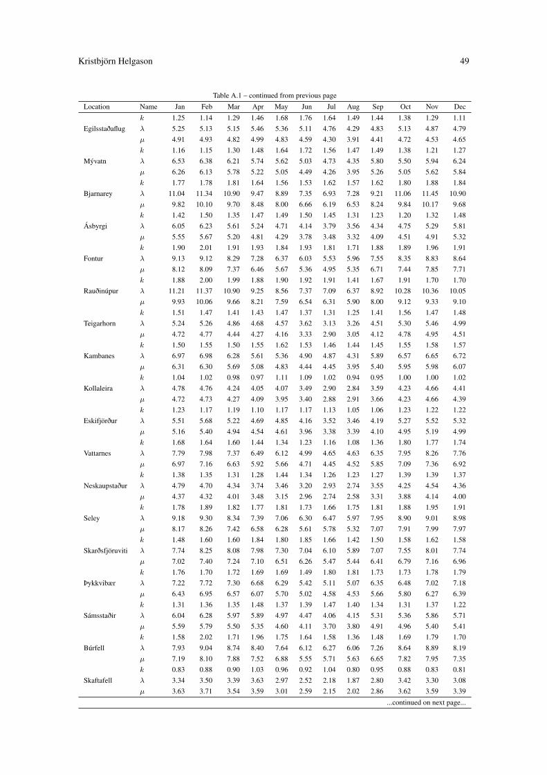
Kristbjörn Helgason 49
Table A.1 – continued from previous page
Location Name Jan Feb Mar Apr May Jun Jul Aug Sep Oct Nov Dec
Egilsstaðaflugk 1.25 1.14 1.29 1.46 1.68 1.76 1.64 1.49 1.44 1.38 1.29 1.11λ 5.25 5.13 5.15 5.46 5.36 5.11 4.76 4.29 4.83 5.13 4.87 4.79µ 4.91 4.93 4.82 4.99 4.83 4.59 4.30 3.91 4.41 4.72 4.53 4.65
Mývatnk 1.16 1.15 1.30 1.48 1.64 1.72 1.56 1.47 1.49 1.38 1.21 1.27λ 6.53 6.38 6.21 5.74 5.62 5.03 4.73 4.35 5.80 5.50 5.94 6.24µ 6.26 6.13 5.78 5.22 5.05 4.49 4.26 3.95 5.26 5.05 5.62 5.84
Bjarnareyk 1.77 1.78 1.81 1.64 1.56 1.53 1.62 1.57 1.62 1.80 1.88 1.84λ 11.04 11.34 10.90 9.47 8.89 7.35 6.93 7.28 9.21 11.06 11.45 10.90µ 9.82 10.10 9.70 8.48 8.00 6.66 6.19 6.53 8.24 9.84 10.17 9.68
Ásbyrgik 1.42 1.50 1.35 1.47 1.49 1.50 1.45 1.31 1.23 1.20 1.32 1.48λ 6.05 6.23 5.61 5.24 4.71 4.14 3.79 3.56 4.34 4.75 5.29 5.81µ 5.55 5.67 5.20 4.81 4.29 3.78 3.48 3.32 4.09 4.51 4.91 5.32
Fonturk 1.90 2.01 1.91 1.93 1.84 1.93 1.81 1.71 1.88 1.89 1.96 1.91λ 9.13 9.12 8.29 7.28 6.37 6.03 5.53 5.96 7.55 8.35 8.83 8.64µ 8.12 8.09 7.37 6.46 5.67 5.36 4.95 5.35 6.71 7.44 7.85 7.71
Rauðinúpurk 1.88 2.00 1.99 1.88 1.90 1.92 1.91 1.41 1.67 1.91 1.70 1.70λ 11.21 11.37 10.90 9.25 8.56 7.37 7.09 6.37 8.92 10.28 10.36 10.05µ 9.93 10.06 9.66 8.21 7.59 6.54 6.31 5.90 8.00 9.12 9.33 9.10
Teigarhornk 1.51 1.47 1.41 1.43 1.47 1.37 1.31 1.25 1.41 1.56 1.47 1.48λ 5.24 5.26 4.86 4.68 4.57 3.62 3.13 3.26 4.51 5.30 5.46 4.99µ 4.72 4.77 4.44 4.27 4.16 3.33 2.90 3.05 4.12 4.78 4.95 4.51
Kambanesk 1.50 1.55 1.50 1.55 1.62 1.53 1.46 1.44 1.45 1.55 1.58 1.57λ 6.97 6.98 6.28 5.61 5.36 4.90 4.87 4.31 5.89 6.57 6.65 6.72µ 6.31 6.30 5.69 5.08 4.83 4.44 4.45 3.95 5.40 5.95 5.98 6.07
Kollaleirak 1.04 1.02 0.98 0.97 1.11 1.09 1.02 0.94 0.95 1.00 1.00 1.02λ 4.78 4.76 4.24 4.05 4.07 3.49 2.90 2.84 3.59 4.23 4.66 4.41µ 4.72 4.73 4.27 4.09 3.95 3.40 2.88 2.91 3.66 4.23 4.66 4.39
Eskifjörðurk 1.23 1.17 1.19 1.10 1.17 1.17 1.13 1.05 1.06 1.23 1.22 1.22λ 5.51 5.68 5.22 4.69 4.85 4.16 3.52 3.46 4.19 5.27 5.52 5.32µ 5.16 5.40 4.94 4.54 4.61 3.96 3.38 3.39 4.10 4.95 5.19 4.99
Vattarnesk 1.68 1.64 1.60 1.44 1.34 1.23 1.16 1.08 1.36 1.80 1.77 1.74λ 7.79 7.98 7.37 6.49 6.12 4.99 4.65 4.63 6.35 7.95 8.26 7.76µ 6.97 7.16 6.63 5.92 5.66 4.71 4.45 4.52 5.85 7.09 7.36 6.92
Neskaupstaðurk 1.38 1.35 1.31 1.28 1.44 1.34 1.26 1.23 1.27 1.39 1.39 1.37λ 4.79 4.70 4.34 3.74 3.46 3.20 2.93 2.74 3.55 4.25 4.54 4.36µ 4.37 4.32 4.01 3.48 3.15 2.96 2.74 2.58 3.31 3.88 4.14 4.00
Seleyk 1.78 1.89 1.82 1.77 1.81 1.73 1.66 1.75 1.81 1.88 1.95 1.91λ 9.18 9.30 8.34 7.39 7.06 6.30 6.47 5.97 7.95 8.90 9.01 8.98µ 8.17 8.26 7.42 6.58 6.28 5.61 5.78 5.32 7.07 7.91 7.99 7.97
Skarðsfjöruvitik 1.48 1.60 1.60 1.84 1.80 1.85 1.66 1.42 1.50 1.58 1.62 1.58λ 7.74 8.25 8.08 7.98 7.30 7.04 6.10 5.89 7.07 7.55 8.01 7.74µ 7.02 7.40 7.24 7.10 6.51 6.26 5.47 5.44 6.41 6.79 7.16 6.96
Þykkvibærk 1.76 1.70 1.72 1.69 1.69 1.49 1.80 1.81 1.73 1.73 1.78 1.79λ 7.22 7.72 7.30 6.68 6.29 5.42 5.11 5.07 6.35 6.48 7.02 7.18µ 6.43 6.95 6.57 6.07 5.70 5.02 4.58 4.53 5.66 5.80 6.27 6.39
Sámsstaðirk 1.31 1.36 1.35 1.48 1.37 1.39 1.47 1.40 1.34 1.31 1.37 1.22λ 6.04 6.28 5.97 5.89 4.97 4.47 4.06 4.15 5.31 5.36 5.86 5.71µ 5.59 5.79 5.50 5.35 4.60 4.11 3.70 3.80 4.91 4.96 5.40 5.41
Búrfellk 1.58 2.02 1.71 1.96 1.75 1.64 1.58 1.36 1.48 1.69 1.79 1.70λ 7.93 9.04 8.74 8.40 7.64 6.12 6.27 6.06 7.26 8.64 8.89 8.19µ 7.19 8.10 7.88 7.52 6.88 5.55 5.71 5.63 6.65 7.82 7.95 7.35
Skaftafellk 0.83 0.88 0.90 1.03 0.96 0.92 1.04 0.80 0.95 0.88 0.83 0.81λ 3.34 3.50 3.39 3.63 2.97 2.52 2.18 1.87 2.80 3.42 3.30 3.08µ 3.63 3.71 3.54 3.59 3.01 2.59 2.15 2.02 2.86 3.62 3.59 3.39
...continued on next page...
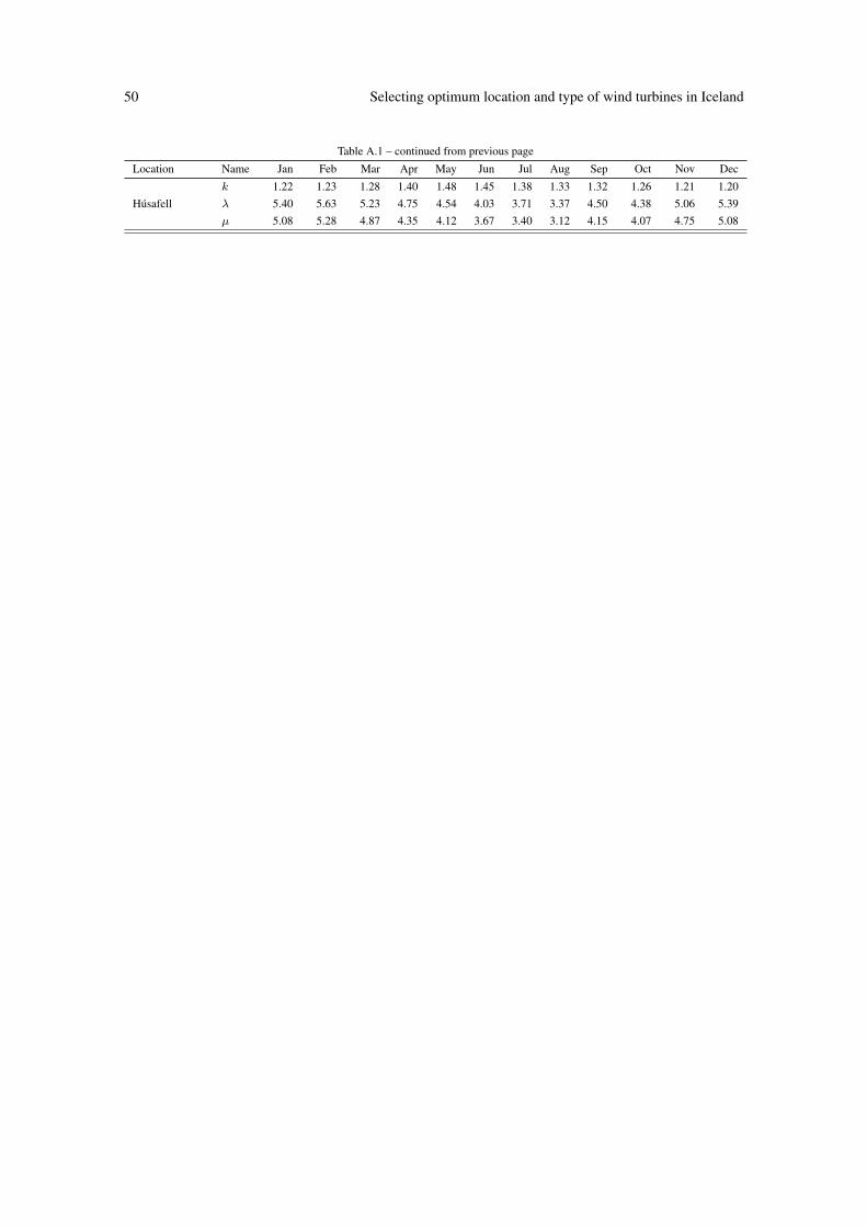
50 Selecting optimum location and type of wind turbines in Iceland
Table A.1 – continued from previous page
Location Name Jan Feb Mar Apr May Jun Jul Aug Sep Oct Nov Dec
Húsafellk 1.22 1.23 1.28 1.40 1.48 1.45 1.38 1.33 1.32 1.26 1.21 1.20λ 5.40 5.63 5.23 4.75 4.54 4.03 3.71 3.37 4.50 4.38 5.06 5.39µ 5.08 5.28 4.87 4.35 4.12 3.67 3.40 3.12 4.15 4.07 4.75 5.08

51
Appendix B
Turbines
Table B.1: Turbine parameters and power in kW at 1-11 m/s
rotor cutout cutin 1 2 3 4 5 6 7 8 9 10 11
AAER_A1650_77m_1650kW 77.0 20.0 3.0 0.0 0.0 0.0 57.0 141.0 258.0 422.0 642.0 919.0 1237.0 1541.0AAER_A1650_82m_1650kW 82.0 20.0 3.0 0.0 0.0 0.0 71.0 173.0 316.0 516.0 781.0 1117.0 1520.0 1651.0
Bonus_82.4m_2.3MW 82.0 25.0 4.0 0.0 0.0 0.0 0.0 153.7 301.2 479.4 731.4 1008.0 1346.1 1745.6Bonus_MkIV_44m_600kW 44.0 25.0 3.0 0.0 0.0 0.0 23.0 48.0 80.0 123.0 177.0 247.0 341.0 431.0
Clipper_C100_100m_2500kW 100.0 25.0 3.0 0.0 0.0 0.0 96.0 221.0 412.0 669.0 993.0 1456.0 1882.0 2235.0Clipper_C89_89m_2500kW 89.0 25.0 3.0 0.0 0.0 0.0 58.0 154.0 301.0 522.0 801.0 1162.0 1603.0 1985.0Clipper_C93_93m_2500kW 93.0 25.0 3.0 0.0 0.0 0.0 58.0 184.0 353.0 581.0 875.0 1272.0 1684.0 2066.0Clipper_C96_96m_2500kW 96.0 25.0 3.0 0.0 0.0 0.0 88.0 206.0 382.0 632.0 971.0 1375.0 1801.0 2154.0
Enercon_E101_101m_3000kW 101.0 25.0 2.5 0.0 0.0 37.0 118.0 258.0 479.0 790.0 1200.0 1710.0 2340.0 2867.0Enercon_E33_33.4m_330kW 33.0 25.0 2.5 0.0 0.0 5.0 13.7 30.0 55.0 92.0 138.0 196.0 250.0 292.0
Enercon_E44_44m_900kW 44.0 25.0 1.0 0.0 1.4 8.0 24.5 53.0 96.0 156.0 238.0 340.0 466.0 600.0Enercon_E48_48m_800kW 48.0 25.0 1.5 0.0 2.0 12.0 32.0 66.0 120.0 191.0 284.0 405.0 555.0 671.0
Enercon_E53_52.9m_800kW 52.0 25.0 1.5 0.0 2.0 14.0 38.0 77.0 141.0 228.0 336.0 480.0 645.0 744.0Enercon_E70_71m_2300kW 71.0 25.0 1.5 0.0 2.0 18.0 56.0 127.0 240.0 400.0 626.0 892.0 1223.0 1590.0
Enercon_E82_E2_82m_2000kW 82.0 25.0 1.5 0.0 3.0 25.0 82.0 174.0 321.0 532.0 815.0 1180.0 1612.0 1890.0Enercon_E82_82m_2300kW 82.0 25.0 2.5 0.0 0.0 25.0 82.0 174.0 321.0 532.0 815.0 1180.0 1580.0 1890.0Enercon_E82_82m_3000kW 82.0 25.0 2.5 0.0 0.0 25.0 82.0 174.0 321.0 532.0 815.0 1180.0 1580.0 1900.0
Gamesa_G52_850kW 52.0 25.0 3.5 0.0 0.0 0.0 27.9 65.2 123.1 203.0 307.0 435.3 564.5 684.6Gamesa_G58_850kW 58.0 21.0 2.5 0.0 0.0 9.7 31.2 78.4 148.2 242.7 368.8 525.3 695.0 796.6Gamesa_G80_2.0MW 80.0 25.0 3.5 0.0 0.0 0.0 66.3 152.0 280.0 457.0 690.0 978.0 1296.0 1598.0Gamesa_G83_2.0MW 83.0 25.0 3.5 0.0 0.0 0.0 65.1 152.4 285.2 470.8 715.8 1024.8 1377.4 1690.8Gamesa_G87_2.0MW 87.0 25.0 3.5 0.0 0.0 0.0 78.6 181.2 335.4 549.8 831.5 1174.8 1528.3 1794.7Gamesa_G90_2.0MW 90.0 21.0 2.5 0.0 0.0 21.3 84.9 197.3 363.8 594.9 900.8 1274.4 1633.0 1863.0
GE_1.6MW 100.0 25.0 3.5 0.0 0.0 0.0 38.0 154.0 405.0 693.0 986.0 1323.0 1506.0 1578.0GE_1.5sl_77m_1500kW 77.0 20.0 3.5 0.0 0.0 0.0 32.0 107.0 230.0 391.0 616.0 895.0 1178.0 1435.0
GE_2.5xl_100m_2500kW 100.0 25.0 3.5 0.0 0.0 0.0 55.0 182.0 391.0 645.0 955.0 1345.0 1855.0 2245.0GE_3.6sl_111m_3600kW 111.0 27.0 3.5 0.0 0.0 0.0 98.0 244.0 451.0 732.0 1110.0 1574.0 2184.0 2721.0
Leitwind_LTW101m_3MW 100.0 25.0 2.5 0.0 0.0 41.0 124.0 257.0 456.0 735.0 1101.0 1537.0 2019.0 2543.0Leitwind_LTW70_1.7MW 70.0 25.0 3.0 0.0 0.0 0.0 58.0 120.0 213.0 344.0 519.0 742.0 1018.0 1327.0
Leitwind_LTW70_2MW 70.0 25.0 3.0 0.0 0.0 0.0 57.0 120.0 214.0 347.0 524.0 749.0 1012.0 1309.0Leitwind_LTW77m_1.5MW 77.0 25.0 3.0 0.0 0.0 0.0 61.0 135.0 248.0 406.0 619.0 877.0 1158.0 1435.0
Leitwind_LTW80_1.5MW 80.0 25.0 3.0 0.0 0.0 0.0 77.0 184.0 330.0 527.0 761.0 993.0 1268.0 1462.0Leitwind_LTW80_1.8MW 80.0 25.0 3.0 0.0 0.0 0.0 80.0 163.0 287.0 460.0 691.0 986.0 1346.0 1749.0
Nordex_N100_2500kW 99.0 20.0 3.0 0.0 0.0 0.0 50.0 211.0 429.0 725.0 1111.0 1583.0 2023.0 2306.0Nordex_N60__1.3MW 60.0 25.0 3.5 0.0 0.0 0.0 25.0 78.0 150.0 234.0 381.0 557.0 752.0 926.0Nordex_N70__1.5MW 70.0 25.0 3.5 0.0 0.0 0.0 24.0 87.0 190.0 329.0 520.0 750.0 1016.0 1284.0Nordex_N90_2500kW 90.0 25.0 3.0 0.0 0.0 0.0 43.0 181.0 374.0 599.0 877.0 1230.0 1626.0 2011.0Nordex_S70_1500kW 70.0 25.0 3.0 0.0 0.0 0.0 24.0 87.0 190.0 329.0 531.0 736.0 1016.0 1284.0Nordex_S77_1500kW 77.0 25.0 3.0 0.0 0.0 0.0 44.0 131.0 244.0 400.0 600.0 854.0 1111.0 1331.0
Siemens_SWT_101m_2.3MW 101.0 25.0 3.5 0.0 0.0 0.0 102.0 252.0 462.0 774.0 1163.0 1583.0 2014.0 2254.0Siemens_SWT_93m_2.3MW 93.0 25.0 3.5 0.0 0.0 0.0 59.0 200.0 400.0 678.0 1011.0 1361.0 1712.0 2012.0
Siemens_SWT_3.6MW 107.0 25.0 3.5 0.0 0.0 0.0 113.0 296.0 523.0 827.0 1159.0 1594.0 2135.0 2788.0Vestas_V90_3MW 90.0 25.0 3.5 0.0 0.0 0.0 77.0 190.0 353.0 581.0 886.0 1273.0 1710.0 2145.0Vestas_80m_2MW 80.0 25.0 3.5 0.0 0.0 0.0 66.0 166.0 288.0 473.0 709.0 1000.0 1316.0 1651.0
Vestas_V_90_GridStreamer_2MW 90.0 25.0 3.5 0.0 0.0 0.0 92.0 213.0 377.0 610.0 925.0 1271.0 1612.0 1896.0Vestas_V52_850kW 52.0 25.0 3.5 0.0 0.0 0.0 19.0 60.0 120.0 200.0 300.0 417.0 539.0 654.0
Vestas_V82_1.65MW 82.0 25.0 3.5 0.0 0.0 0.0 38.0 144.0 307.0 510.0 762.0 1035.0 1300.0 1507.0

52 Selecting optimum location and type of wind turbines in Iceland
Table B.2: Turbine power output in kW at 12-28 m/s
turbine.shortname 12 13 14 15 16 17 18 19 20 21 22 23 24 25 26 27 28
AAER_A1650_77m 1651 1651 1651 1651 1651 1651 1651 1651 1651 0 0 0 0 0 0 0 0AAER_A1650_82m 1651 1651 1651 1651 1651 1651 1651 1651 1651 0 0 0 0 0 0 0 0Bonus_82.4m_2. 2035 2200 2274 2299 2311 2311 2311 2311 2311 2311 2311 2311 2311 2305 0 0 0Bonus_MkIV_44m 497 551 583 603 609 608 595 577 549 525 512 497 478 460 0 0 0Clipper_C100_1 2419 2485 2500 2500 2500 2500 2500 2500 2500 2500 2500 2500 2500 2500 0 0 0Clipper_C89_89 2265 2412 2485 2500 2500 2500 2500 2500 2500 2500 2500 2500 2500 2500 0 0 0Clipper_C93_93 2338 2448 2500 2500 2500 2500 2500 2500 2500 2500 2500 2500 2500 2500 0 0 0Clipper_C96_96 2382 2478 2500 2500 2500 2500 2500 2500 2500 2500 2500 2500 2500 2500 0 0 0Enercon_E101_1 3034 3050 3050 3050 3050 3050 3050 3050 3050 3050 3050 3050 3050 3050 0 0 0Enercon_E33_33 320 335 335 335 335 335 335 335 335 335 335 335 335 335 0 0 0Enercon_E44_44 710 790 850 880 905 910 910 910 910 910 910 910 910 910 0 0 0Enercon_E48_48 750 790 810 810 810 810 810 810 810 810 810 810 810 810 0 0 0Enercon_E53_52 780 810 810 810 810 810 810 810 810 810 810 810 810 810 0 0 0Enercon_E70_71 1900 2080 2230 2300 2310 2310 2310 2310 2310 2310 2310 2310 2310 2310 0 0 0Enercon_E82_E2 2000 2050 2050 2050 2050 2050 2050 2050 2050 2050 2050 2050 2050 2050 0 0 0Enercon_E82_82 2100 2250 2350 2350 2350 2350 2350 2350 2350 2350 2350 2350 2350 2350 0 0 0Enercon_E82_82 2200 2480 2700 2850 2950 3020 3020 3020 3020 3020 3020 3020 3020 3020 0 0 0Gamesa_G52_850 780 841 848 849 850 850 850 850 850 850 850 850 850 850 0 0 0Gamesa_G58_850 836 847 849 850 850 850 850 850 850 850 0 0 0 0 0 0 0Gamesa_G80_2.0 1818 1935 1980 1995 1999 2000 2000 2000 2000 2000 2000 2000 2000 2000 0 0 0Gamesa_G83_2.0 1882 1964 1990 1998 1999 2000 2000 2000 2000 2000 2000 2000 2000 2000 0 0 0Gamesa_G87_2.0 1931 1981 1995 1999 2000 2000 2000 2000 2000 2000 2000 2000 2000 2000 0 0 0Gamesa_G90_2.0 1960 1990 1998 2000 2000 2000 2000 2000 2000 2000 0 0 0 0 0 0 0GE_1.6MW 1600 1600 1600 1600 1600 1600 1600 1600 1600 1600 1600 1600 1600 1600 0 0 0GE_1.5sl_77m_1 1500 1500 1500 1500 1500 1500 1500 1500 1500 0 0 0 0 0 0 0 0GE_2.5xl_100m_ 2418 2500 2500 2500 2500 2500 2500 2500 2500 2500 2500 2500 2500 2500 0 0 0GE_3.6sl_111m_ 3148 3417 3563 3600 3600 3600 3600 3600 3600 3600 3600 3600 3600 3600 3600 3600 0Leitwind_LTW10 3000 3000 3000 3000 3000 3000 3000 3000 3000 3000 3000 3000 3000 3000 0 0 0Leitwind_LTW70 1700 1700 1700 1700 1700 1700 1700 1700 1700 1700 1700 1700 1700 1700 0 0 0Leitwind_LTW70 1625 1900 2000 2000 2000 2000 2000 2000 2000 2000 2000 2000 2000 2000 0 0 0Leitwind_LTW77 1500 1500 1500 1500 1500 1500 1500 1500 1500 1500 1500 1500 1500 1500 0 0 0Leitwind_LTW80 1500 1500 1500 1500 1500 1500 1500 1500 1500 1500 1500 1500 1500 1500 0 0 0Leitwind_LTW80 1800 1800 1800 1800 1800 1800 1800 1800 1800 1780 1760 1740 1720 1700 0 0 0Nordex_N100_25 2458 2500 2500 2500 2500 2500 2500 2500 2500 0 0 0 0 0 0 0 0Nordex_N60__1. 1050 1159 1249 1301 1306 1292 1283 1282 1288 1292 1300 1313 1344 1344 0 0 0Nordex_N70__1. 1426 1500 1500 1500 1500 1500 1500 1500 1500 1500 1500 1500 1500 1500 0 0 0Nordex_N90_250 2354 2450 2493 2503 2514 2514 2514 2514 2514 2514 2514 2500 2500 2500 0 0 0Nordex_S70_150 1426 1500 1500 1500 1500 1500 1500 1500 1500 1500 1500 1500 1500 1500 0 0 0Nordex_S77_150 1476 1500 1500 1500 1500 1500 1500 1500 1500 1500 1500 1500 1500 1500 0 0 0Siemens_SWT_10 2300 2300 2300 2300 2300 2300 2300 2300 2300 2300 2300 2300 2300 2300 0 0 0Siemens_SWT_93 2208 2300 2300 2300 2300 2300 2300 2300 2300 2300 2300 2300 2300 2300 0 0 0Siemens_SWT_3. 3285 3485 3564 3600 3600 3600 3600 3600 3600 3600 3600 3600 3600 3600 0 0 0Vestas_V90_3MW 2544 2837 2965 2995 3000 3000 3000 3000 3000 3000 3000 3000 3000 3000 0 0 0Vestas_80m_2MW 1860 1968 2000 2000 2000 2000 2000 2000 2000 2000 2000 2000 2000 2000 0 0 0Vestas_V_90_Gr 2000 2000 2000 2000 2000 2000 2000 2000 2000 2000 2000 2000 2000 2000 0 0 0Vestas_V52_850 754 822 850 850 850 850 850 850 850 850 850 850 850 850 0 0 0Vestas_V82_1.6 1593 1637 1650 1650 1650 1650 1650 1650 1650 1650 1650 1650 1650 1650 0 0 0

53
Appendix C
Distance from location to nearestsubstation
Table C.1: Distance from weather stations to nearest substation in km
Station Distance Substation
2738 Bolungarvík 0.4 Bolungarvík
1479 Korpa 0.8 Korpa
5981 Eskifjörður 1.2 Eskifjörður
5872 Teigarhorn 1.4 Teigar
5990 Neskaupstaður 1.4 Neskaupstaður
2642 Ísafjörður 2.0 Ísafjörður
4180 Seyðisfjörður 2.3 Seyðisfjörður
4271 Egilsstaðaflugvöllur 2.4 Eyvindará
1475 Reykjavík 2.8 Hnoðraholt
6430 Búrfell 4.5 Búrfell
1477 Reykjavíkurflugvöllur 4.5 Hnoðraholt
1473 Straumsvík 5.2 Öldugata
2631 Flateyri 6.1 Breiðadalur
5975 Kollaleira 6.3 Stuðlar
6222 Sámsstaðir 6.3 Hvolsvöllur
1779 Hvanneyri 7.4 Vatnshamar
2646 Súðavík 7.8 Ísafjörður
4614 Ásbyrgi 8.1 Lindabrekka
2319 Patreksfjörður 8.1 Keldeyri
1578 Skrauthólar 8.6 Korpa
4060 Hallormsstaður 9.0 Hryggstekkur
...continued on next page...
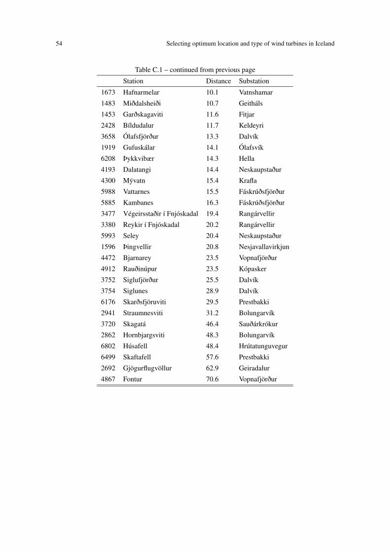
54 Selecting optimum location and type of wind turbines in Iceland
Table C.1 – continued from previous page
Station Distance Substation
1673 Hafnarmelar 10.1 Vatnshamar
1483 Miðdalsheiði 10.7 Geitháls
1453 Garðskagaviti 11.6 Fitjar
2428 Bíldudalur 11.7 Keldeyri
3658 Ólafsfjörður 13.3 Dalvík
1919 Gufuskálar 14.1 Ólafsvík
6208 Þykkvibær 14.3 Hella
4193 Dalatangi 14.4 Neskaupstaður
4300 Mývatn 15.4 Krafla
5988 Vattarnes 15.5 Fáskrúðsfjörður
5885 Kambanes 16.3 Fáskrúðsfjörður
3477 Végeirsstaðir í Fnjóskadal 19.4 Rangárvellir
3380 Reykir í Fnjóskadal 20.2 Rangárvellir
5993 Seley 20.4 Neskaupstaður
1596 Þingvellir 20.8 Nesjavallavirkjun
4472 Bjarnarey 23.5 Vopnafjörður
4912 Rauðinúpur 23.5 Kópasker
3752 Siglufjörður 25.5 Dalvík
3754 Siglunes 28.9 Dalvík
6176 Skarðsfjöruviti 29.5 Prestbakki
2941 Straumnesviti 31.2 Bolungarvík
3720 Skagatá 46.4 Sauðárkrókur
2862 Hornbjargsviti 48.3 Bolungarvík
6802 Húsafell 48.4 Hrútatunguvegur
6499 Skaftafell 57.6 Prestbakki
2692 Gjögurflugvöllur 62.9 Geiradalur
4867 Fontur 70.6 Vopnafjörður

55
Appendix D
Computer Codes
# Load packages
library(fitdistrplus)
library('R.matlab')library('zoo')library('chron')library('reshape')library('RgoogleMaps')library('RSvgDevice')library('Hmisc')library("mixdist")
library(ggplot2)
library('ffbase')library('xtable')library(mapdata)
library(RSQLite)
install.packages('directlabels')library('directlabels')
## importa stödvum og laga nöfn á theim
stodvar <-read.delim(" /Documents/MATLAB/FINAL/wep/sta.stod_leidr",stringsAsFactor=FALSE)stodvar$EIG <- factor(stodvar$EIG)selected <- readMat(' /Dropbox/Skoli_vor2012/FINAL/DATA/HIwind/selected.mat')selected <- as.numeric(selected$selected)lowstodvar <- stodvar[stodvar$STOD %in% selected,]
lowstodvar$NAFN <- trim(lowstodvar$NAFN)lowstodvar$NAFN <- gsub(' ','_', lowstodvar$NAFN)lowstodvar$NAFN <- trim(lowstodvar$NAFN)
## Breyti hnitum svo thau séu í tugabrotum í vectorum
hnitasplit <- gsub("'","",lowstodvar$BREIDD)hnitasplit <- strsplit(as.character(hnitasplit),"°")
hnitasplit <- unlist(hnitasplit)
hnitasplit <- matrix(as.numeric(hnitasplit),ncol=2,byrow=TRUE)
hnitasplit[,2] <- hnitasplit[,2]/60
breidd2 <- hnitasplit[,1]+hnitasplit[,2]
hnitasplit <- gsub("'","",lowstodvar$LENGD)
56 Selecting optimum location and type of wind turbines in Iceland
hnitasplit <- strsplit(as.character(hnitasplit),"°")
hnitasplit <- unlist(hnitasplit)
hnitasplit <- matrix(as.numeric(hnitasplit),ncol=2,byrow=TRUE)
hnitasplit[,2] <- hnitasplit[,2]/60
lengd2 <- (hnitasplit[,1]+hnitasplit[,2])*-1
##------------ Connect to SQLite database
drv <- dbDriver("SQLite")
con <- dbConnect(drv,' /Documents/winddatabase')dbListTables(con)
dbDisconnect(con)
# --------- Database import, bara gera í fyrsta skiptid
drv <- dbDriver("SQLite")
consql <- function(db)dbcon <- dbConnect(dbDriver("SQLite"),file.path(' /Documents/',db))return(dbcon)
con <- consql('winddatabase')
for (i in selected)tablename <- paste('table',i,sep='_')windfile <- paste(' /Documents/MATLAB/wep/M-Files/OUT/gogn/',i,'.txt',sep='')stodin <- read.delim(windfile,header=FALSE,sep='\t',
colClasses=c('NULL','integer','integer','integer','integer','integer','numeric'))names(stodin) <- c('year','month','day','hour','minute','wind')dbWriteTable(con,tablename,stodin, row.names=FALSE,overwrite=TRUE)
rm(stodin)
gc()
#---------- Function to get one station
getOneStation <- function(con,station)q <- paste('SELECT * FROM table',station,sep='_')result <- dbGetQuery(con,q)
return(result)
#---------- Function: Weibull per manud per stod
monthWeibull <- function (p) manstod <- einstod[einstod$month==p,"wind"]fit.einstod.man <- fitdist(einstod[einstod$month==p,"wind"]+0.0001,
'weibull',method='mle')print(plot(fit.einstod.man))
month <- c(fit.einstod.man$estimate,'sd'=fit.einstod.man$sd,mu=mean(manstod),sigma=sd(manstod))
month <- c(unlist(month[1:6]),aic_value=fit.einstod.man$aic)return(month)
#------ Load one station into memory at a time and analyze
windList <- list()
windMatrix <- matrix(ncol=7,nrow=12)
colnames(windMatrix) <- c('shape','scale','sd.shape','sd.scale','mu','sigma','aic_value' )
Kristbjörn Helgason 57
con <- dbConnect(drv,' /Documents/winddatabase')
for (i in 1:nrow(lowstodvar))windtable <- paste('table',lowstodvar$STOD[i],sep='_')einstod <- dbReadTable(con,windtable)
cat("Station:",lowstodvar$STOD[i],lowstodvar$NAFN[i],"\n")windMatrix <- t(sapply(1:12,monthWeibull))
windList[[lowstodvar$NAFN[i]]] <- windMatrix
einstod <- NULL
names(windList) <- trim(names(windList))
copy.windList <- windList
copy.windMatrix <- windMatrix
#Get AVG wind speed for each oation
windAvg <- data.frame('Station'=c(1,1),'Mean.wind'=c(1,1))for (i in 1:nrow(lowstodvar[,]))s <- lowstodvar$NAFN[i]w <- as.numeric(dbGetQuery(con,paste('SELECT AVG( wind ) FROM
table',lowstodvar$STOD[i],sep='_')))windAvg[i,] <- c(s,w)
#set medalvind í töflu
windAvg$Mean.wind <- round(as.numeric(windAvg$Mean.wind),2)windAvg <- cbind(windAvg,lengd2,breidd2)
windOrdAvg <- windAvg[order(windAvg$Mean.wind,decreasing=TRUE),]#mesti medalvindur:
maxwind <- ceiling(max(sapply(windList[1:49],function(x) x[,5])))
#melta töfluna til ad plotta í ggplot, fyrir hverja station
plotMeanWind <- function(st)a <- data.frame(sapply(windList[st],function(x) x[,5]))
names(a) <- names(windList)[st]
b <- melt.data.frame(a)
#Plotta medalvind mánada fyrir n stödvar
rtext <- data.frame(x=12,y=as.numeric(a[12,]),label=as.character(names(a)))
gg <- ggplot()+xlim(c(1,13.9))+#ylim(c(1.8,maxwind))+geom_line(data=b,aes(x=1:12, y=value,col=variable),alpha=0.5,size=0.6)+
labs(x='Month',y='Mean wind speed [m/s]')+scale_color_discrete(b$variable,h=c(10,360),h.start=90, l=57)+
scale_x_date(format = "%b") +
theme_bw()+opts(legend.position='none')
print(gg)
top25 <- order(windAvg$Mean.wind,decreasing=TRUE)[1:25]plotMeanWind(top25)
ggsave('fig/meanWind1_25low.pdf',width=9,height=7)
plotMeanWind(order(windAvg$Mean.wind,decreasing=TRUE)[26:49])ggsave('fig/meanWind26_49.pdf',width=9,height=9)
#---------SIMULATION------daysinmonth <- c(31,28,31,30,31,30,31,31,30,31,30,31)
58 Selecting optimum location and type of wind turbines in Iceland
n=50000
st <- 33
mon <- 12
simulateWind <- function(st,mon,n)sh.wei <- windList[[st]][mon,1]
sc.wei <- windList[[st]][mon,2]
p <- runif(n)
weisim <- qweibull(p=p,shape=sh.wei,scale=sc.wei)
return(weisim)
simulateWindAnti <- function(st,mon,n)sh.wei <- windList[[st]][mon,1]
sc.wei <- windList[[st]][mon,2]
p <- runif(n/2)
p <- c(p,1-p)
weisim <- qweibull(p=p,shape=sh.wei,scale=sc.wei)
return(weisim)
simulateEnergy <- function(tur,mon,wind)cutin <- turbines['cutin',tur]cutout <- turbines['cutout',tur]simwind1 <- wind*powerLaw[tur]
simwind <- data.frame(weib=simwind1, round.down=floor(simwind1),
round.up=ceil(simwind1))
simwind[simwind$weib>30,] <- 0
simwind <- cbind(simwind,pdn=turbines[simwind$round.down+3,tur],pup=turbines[simwind$round.up+3,tur])
simwind$pdiff <- simwind$pup-simwind$pdnsimwind$pdiff[simwind$pdiff<0] <- 0
simwind$totpow <- with(simwind,pdn+weib %% 1 * pdiff)
simwind$totpow[simwind$weib<cutin] <- 0
simwind$totpow[simwind$weib>cutout] <- 0
#MWh framl í mánudinum:
monenergy <- mean(simwind$totpow)*24*daysinmonth[mon]/1000return(monenergy) #list(weisimall,monenergy)) simwind$totpow)
#---plot simulation
bjar <- getOneStation(con,lowstodvar$STOD[lowstodvar$NAFN=='Bjarnarey'])bjarNov <- bjar[bjar$month==12,]mon=10
st=32
weisim <- simulateWind(st,mon,50000)
weisim2 <- data.frame(variable='Simulated wind', wind=simulateWind(st,mon,50000))
WindBjar <- data.frame(variable='Measured wind',wind=bjarNov$wind)WindSimCom <- rbind(weisim2,WindBjar)
histname <- paste(lowstodvar$NAFN[st],'in',month.abb[mon])pdf('fig/SimWeiHist.pdf',width=7,height=6)hist(bjar$wind[bjar$month==10],main=histname,xlim=c(0,30),ylim=c(0,0.075),cex.main=1,
xlab='Wind [m/s]',freq=FALSE, border='grey40',breaks=seq(0,40,1),cex.lab=1.2,cex.main=1.4)
x=seq(0,30,0.1)

Kristbjörn Helgason 59
curve(dweibull(x,scale=windList[[st]][mon,2], shape=windList[[st]][mon,1]),add=TRUE,
col='red')points(density(weisim), type='l',col='navy',lty='dashed',lwd=1.6)legend(x=14,y=max(density(weisim)$y),legend=c('Measured wind','Density of simulated
wind','Weibull curve'),cex=1,pch=c('l','-','_'), col=c('grey40','navy','red'),
box.col='white')dev.off()
rm(bjar)
############# Power and energy simulation ###########
simulatePowerMonth <- function(st,mon,n)wind <- simulateWind(st,mon,n)
#simulate power for all turbines
powergen <- sapply(1:ncol(turbines),simulateEnergy,mon=mon,wind=wind)
#cat(month.abb[mon],'-')return(powergen)
simulateYear <- function(st,n)cat(st,'-')tmp <- sapply(1:12,simulatePowerMonth,st=st,n=n)
tmp <- cbind(tmp,rowSums(tmp))
return(tmp)
#simulate all stations for n instances
simEnAllStations <- vector(mode='list',length=48)for (i in 1:48) simEnAllStations[[i]] <- matrix(nrow=47,ncol=13)
timestamp()
simEnAllStations <- lapply(1:48,simulateYear,n=50000)
timestamp()
names(simEnAllStations) <- lowstodvar$NAFN#copy.simEnAllStations <- simEnAllStations
simAllUnlist <- sapply(simEnAllStations[1:48],function(x) x[,-13])
#simAllUnlist50 <- sapply(simEnAllStations50000[1:48],function(x) x[,-13])
#simAllUnlist5 <- sapply(simEnAllStations500[1:48],function(x) x[,-13])
plot(density(simAllUnlist),lty=1, col='red')points(density(simAllUnlist50),type='l',lty=2, col='green')points(density(simAllUnlist5),type='l',lty=3)
############## Annual Energy calculations: ###########Reikna annual energy output fyrir allar location
energyAll <- data.frame('station'=c(),'turbine'=c(),'energy'=c())
for(i in lowstodvar$NAFN)en1 <- as.vector(x=simEnAllStations[[i]][,13])+turbines[4,]
en1 <- t(en1/1000) #from MWh to GWh
en1 <- en1[order(en1,decreasing=TRUE),]
en1df <- data.frame(turbine=factor(names(en1),ordered=FALSE),energy=en1)
energyAll <- rbind(energyAll,cbind(names(simEnAllStations[i]),en1df))
row.names(energyAll) <- NULL

60 Selecting optimum location and type of wind turbines in Iceland
names(energyAll)[1] <- 'station'
energyMeanAll <- sapply(lowstodvar$NAFN,function(x)mean(energyAll$energy[energyAll$station==x]))energyMeanOrdNames <- names(sort(energyMeanAll,decreasing=TRUE))
energyMeanTur <- sapply(names(turbines),function(x)
mean(energyAll$energy[energyAll$turbine==x]))energyMeanOrdTur <- names(sort(energyMeanTur,decreasing=TRUE))
energyMax <-data.frame(station=energyAll$station[order(energyAll$energy,decreasing=TRUE)],
energy=round(sort(energyAll$energy,decreasing=TRUE),1))
##-#-#-# #-Plot heatmap of annual energy for al stations
fill_factor <- cut(round(energyAll$energy,1), breaks=c(0,2,4,6,8,10,14,19))
ggplot(data=energyAll)+
geom_tile(aes(station,turbine,fill=fill_factor))+theme_bw()+opts(axis.text.x=theme_text(hjust=1, vjust=1,
angle=50,size=8.5),axis.text.y=theme_text(size=9,hjust=1))+scale_fill_brewer(name='Energy [GWh]',palette='YlGn')+scale_y_discrete(name='', limits=energyMeanOrdTur)+
scale_x_discrete(name='',limits=energyMeanOrdNames)+coord_flip()ggsave('fig/energyAllOrd.pdf',width=10.3,height=9.5)
############## CF calculations: ############Reikna capacity factor fyrir allar location
cfAll <- data.frame('station'=c(),'turbine'=c(),'cf'=c())
for(i in lowstodvar$NAFN)cf1 <- as.vector(x=simEnAllStations[[i]][,13])/turbines[34,]
cf1 <- t(cf1)
cf1 <- cf1[order(cf1,decreasing=TRUE),]
cf1df <- data.frame(turbine=factor(names(cf1),ordered=FALSE),CF=cf1)
#cf1df <- cf1df[-c(55,64),]
#cf1df <- droplevels(cf1df$turbine)pdf(paste('fig/CapFactor2/cf',names(simEnAllStations[i]),'.pdf',sep=''),7,7)color=as.numeric(turbines['rotor',match(cf1df$turbine,names(turbines))])print(ggplot(data=cf1df) + xlab('Turbines') + ylab('Capacity factor') + theme_bw()+geom_point(aes(x=turbine,y=CF, color=color),size=3)+
opts(title=paste('Efficiency of turbines at',names(simEnAllStations[i])))+scale_color_continuous(name='Rotor size [m]',breaks=seq(20,100,by=15), low =
"yellow",high = "red") +
scale_x_discrete(limits=rev(names(cf1)))+scale_size(guide = 'none')+coord_flip()+opts(axis.text.y = theme_text(size =
8,hjust=1)))
dev.off()
cfAll <- rbind(cfAll,cbind(names(simEnAllStations[i]),cf1df))
row.names(cfAll) <- NULL
names(cfAll)[1] <- 'station'
cfMeanAll <- sapply(lowstodvar$NAFN,function(x) mean(cfAll$CF[cfAll$station==x]))cfMeanOrdNames <- names(sort(cfMeanAll,decreasing=TRUE))
cfMeanTur <- sapply(names(turbines),function(x) mean(cfAll$CF[cfAll$turbine==x]))cfMeanOrdTur <- names(sort(cfMeanTur,decreasing=TRUE))
Kristbjörn Helgason 61
##-#-#-# #-Plot heatmap of all CF for al stations
fill_factor <- cut(round(cfAll$CF*100), breaks=seq(0,70,10))
ggplot(data=cfAll)+
geom_tile(aes(station,turbine,fill=fill_factor))+theme_bw()+opts(axis.text.x=theme_text(hjust=1, vjust=1,
angle=50,size=8.5),axis.text.y=theme_text(size=9,hjust=1))+scale_fill_brewer(name='Efficiency [%]',palette='OrRd')+scale_y_discrete(name='', limits=cfMeanOrdTur)+
scale_x_discrete(name='',limits=cfMeanOrdNames)+coord_flip()ggsave('fig/cfAllOrd.pdf',width=10.3,height=9.5)
### Tek út 5 hæstu, set upp í töflu og plott saman á graf
top5cf <- cfMeanOrdNames[1:5,drop=TRUE]
cfTop5 <- subset(cfAll,subset=station %in% top5cf)
cfTop5$station <- cfTop5$station[,drop=TRUE]levels(cfTop5$station) <- top5cf
colcf <- as.numeric(turbines['rotor',match(cfTop5$turbine,names(turbines))])
ggplot(cfTop5)+geom_point(aes(x=turbine,y=CF, color=colcf),size=2.5)+
facet_grid(station ˜ .)+
scale_color_continuous(name='Rotor size [m]',breaks=seq(20,100,by=15), low =
"yellow",high = "red")+
scale_x_discrete(name='',limits=unique(cfAll$turbine))+scale_size(guide = 'none')+theme_bw()+opts(axis.text.x = theme_text(size =
8,angle=53,hjust=1,vjust=1),legend.position='top')ggsave('fig/cfTop5.pdf',width=8,height=10)
# Geri töflu yfir 10 stadi med Hæst CF, plottad á kort í mapplots.R
top10cf <- cfMeanOrdNames[1:10,drop=TRUE]
cfTop10all <- subset(cfAll,subset=station %in% top10cf)
cfTop10all$turbine <- as.character(cfTop10all$turbine)cfTop10all$station <- as.character(cfTop10all$station)cfTop10 <- sapply(top10cf, function(x) subset(cfTop10all,
subset= CF==max(CF[station==x][CF[station==x] !=
max(CF[station==x])])))
cfTop10 <- data.frame(t(cfTop10), row.names=NULL)
cfTop10$CF <- as.numeric(cfTop10$CF)cfTop10 <- cfTop10[order(cfTop10$CF, decreasing=TRUE),]
cfTop10$breidd <-as.numeric(sapply(cfTop10$station,function(x)lowstodvar$breidd2[lowstodvar$NAFN==x]))cfTop10$lengd <-as.numeric(sapply(cfTop10$station,function(x)lowstodvar$lengd2[lowstodvar$NAFN==x]))
#install.packages('geosphere')require(maptools)
kmldata <- getKMLcoordinates(
' /Dropbox/Skoli_vor2012/FINAL/DATA/LandsnetTengivirki/TengivirkiLandsnets2.kml',ignoreAltitude=TRUE)
tengivirki <- matrix(unlist(kmldata),ncol=2,byrow=TRUE)
station.longlat <- data.frame(lengd2,breidd2)
row.names(station.longlat) <- lowstodvar$STOD

62 Selecting optimum location and type of wind turbines in Iceland
tengivirki.longlat <-data.frame(long=as.numeric(tengivirki[,1]),lat=as.numeric(tengivirki[,2]))
#tmp <- read.clipboard.csv(header=FALSE,as.is=TRUE)
#tmp <- sub("\n+.*",'',tmp$V1)#dput(tmp)tengivirki.nofn <- c("Öldugata", "Vopnafjörður", "Varmahlíð", "Vatnshamar",
"Vestmannaeyjar", "Vegamót", "Vogaskeið", "Grundarfjörður",
"Ólafsvík", "Glerárskógafjall", "Hrútatunguvegur", "Geiradalur",
"Keldeyri", "Mjólká", "Ísafjörður", "Breiðadalur", "Bolungarvík",
"Blanda", "Laxárvatn", "Sauðárkrókur", "Rangárvellir", "Dalvík",
"Húsavík", "Laxá", "Krafla", "Lindabrekka", "Lagarfossvirkjun",
"Eyvindará", "Seyðisfjörður", "Neskaupstaður", "Eskifjörður",
"Fáskrúðsfjörður", "Fljótsdalur", "Stuðlar", "Hryggstekkur",
"Teigar", "Hólar", "Sigalda", "Vatnsfell", "Hrauneyjafoss",
"Prestbakki", "Sultartangi", "Búrfell", "Hvolsvöllur", "Hella",
"Flúðir", "Selfoss", "Hveragerði", "Nesjavallavirkjun", "Rimakot",
"Sog", "Hamranes", "Svartsengi", "Reykjanes",
"Fitjar", "Rauðimelur", "Korpa", "Hnoðraholt", "Geitháls",
"A12", "Akranes","Kópasker")
tengivirki <- cbind(tengivirki,' '=tengivirki.nofn)
#This function computes the distance on the surface of the earth between two points
#point1 and point2, each of the form (Longitude, Latitude)
geodetic.distance <- function(point1, point2)R <- 6370
p1rad <- point1 * pi/180
p2rad <- point2 * pi/180
d <-sin(p1rad[2])*sin(p2rad[2])+cos(p1rad[2])*cos(p2rad[2])*cos(abs(p1rad[1]-p2rad[1]))
d <- acos(d)
R*d
detect.distance.tonext <- function(point)dist <- vector()
for(i in 1:nrow(tengivirki)) dist[i] <-geodetic.distance(point,tengivirki.longlat[i,])
mindist <- min(unlist(dist))
minnafn <- tengivirki[which.min(unlist(dist)),3]
result <- data.frame(dist=mindist,'tengivirki'=minnafn)return(result)
#keyra detect.dist yfir allar stödvar
shortest.dist <- apply(station.longlat,1,detect.distance.tonext)
shdistframe <- data.frame(shortest.dist)
mintengivirki <- t(as.vector(shdistframe[grep('.tengivirki',names(shdistframe))]))row.names(mintengivirki) <- gsub('.tengivirki','',row.names(mintengivirki))row.names(mintengivirki) <- gsub('X','',row.names(mintengivirki))mindisttoteng <- t(as.vector(shdistframe[grep('.dist',names(shdistframe))]))row.names(mindisttoteng) <- gsub('.dist','',row.names(mindisttoteng))mintenging <- data.frame(mintengivirki,mindisttoteng,'Station'=lowstodvar$NAFN)names(mintenging)[1:2] <- c('Substation','Distance')minTafla <- xtable(mintenging[order(mintenging[,2]),c(3,2,1)],digits=1,
tabular.environment='longtable',floating=FALSE)
Kristbjörn Helgason 63
print.xtable(minTafla,file=' /Dropbox/Skoli_vor2012/FINAL/THESIS/MScThesis/tables/minDistTable.txt')
shdist <- unlist(shortest.dist,recursive=FALSE)
shdist <- shdist[seq(1,length(shdist),2)]
tmp <- data.frame('dist'=unlist(shortest.dist))shortestdist <- subset(tmp,grepl(".dist",row.names(tmp)))
######## Cost of energy ################ Constants
r=0.075; b=0.075; infl=0
N=20; L=20
CRF=r/(1-(1+r)^(-N))k1=1/(1+r)
k2=(1+infl)/(1+r)
### Functions
#capital cost
CcFun <- function(stnum,tur)
460*(turbines['rotor',tur]/2)^2*pi+80000*mintenging$Distance[rownames(mintenging)==stnum]#Annual production in kWh
annual.kWh <- function(stnum,tur)stname <- lowstodvar$NAFN[lowstodvar$STOD==stnum]simEnAllStations[[stname]][tur,13]*1000
#Present value of series of payments
Y <- function(k,l)(k-k^(l+1))/(1-k)
#Cost of energy, leverized
COELfun <- function(stnum,tur)Cc=CcFun(stnum,tur)
OMc=annual.kWh(stnum,tur)*0.0189+26000
Pd=0.1*Cc
Pa=(Cc-Pd)*CRF
NPVc <- Pd+Pa*Y(k1,N)+OMc*Y(k2,L)
COEL <- NPVc*CRF/annual.kWh(stnum,tur)
return(COEL)
COELallTur <- data.frame('turbine'=names(turbines))COELall <- list()
for(i in lowstodvar$STOD)stname <- lowstodvar$NAFN[lowstodvar$STOD==i]COELallTur$COE <- sapply(1:ncol(turbines),COELfun,stnum=i)
COELall[[stname]] <- COELallTur
COELallUnlist <- sapply(COELall[1:48],function(x) x[,2])
rownames(COELallUnlist) <- names(turbines)
COELmelt <- melt(COELallUnlist)
names(COELmelt)[1:2] <- c('turbine','station')
coeMeanAll <- sapply(lowstodvar$NAFN,function(x)mean(COELmelt$value[COELmelt$station==x]))

64 Selecting optimum location and type of wind turbines in Iceland
coeMeanOrdNames <- names(sort(coeMeanAll,decreasing=FALSE))
coeMeanTur <- sapply(names(turbines),function(x)
mean(COELmelt$value[COELmelt$turbine==x]))coeMeanOrdTur <- names(sort(coeMeanTur,decreasing=FALSE))
###-#-# Plot heatmap showing all locations and turbines
fill_factor <- cut(round(COELmelt$value*100,2), breaks=c(4,5,6,7,9,12,15,25,50))
ggplot(data=COELmelt)+
geom_tile(aes(station,turbine,fill=fill_factor))+theme_bw()+opts(axis.text.x=theme_text(hjust=1, vjust=1,
angle=50,size=8.5),axis.text.y=theme_text(size=9,hjust=1))+scale_fill_brewer(name='COE [cent EUR]',palette='YlGnBu', na.value = 'grey20')+scale_y_discrete(name='',limits=coeMeanOrdTur)+scale_x_discrete(name='',limits=coeMeanOrdNames)+coord_flip()
ggsave('fig/coeAllOrd.pdf',width=10.3,height=9.5)
### Tek út 5 hæstu, set upp í töflu og plott saman á graf
top5coe <- coeMeanOrdNames[1:5,drop=TRUE]
coeTop5 <- subset(COELmelt,subset=station %in% top5coe)
coeTop5$station <- coeTop5$station[,drop=TRUE]levels(coeTop5$station) <- top5coe
#rada turb eftir cost röd í tilviki gardskagavita
coeTurbOrd <- subset(coeTop5,subset=station==top5coe[1])#,select=turbine[order(value)])coeTurbOrd <- with(coeTurbOrd,turbine[order(value)])
#library('gtools')#colcoe <-quantcut(as.numeric(turbines['rotor',match(coeTop5$turbine,names(turbines))]),q=seq(0,1,by=0.2))
colcoe <- as.numeric(turbines['rotor',match(coeTop5$turbine,names(turbines))])
ggplot(coeTop5)+geom_point(aes(x=turbine,y=value*100,color=colcoe),size=2.5)+ylim(c(4,10))+
facet_grid(station ˜ ., scale='free_y')+#coord_trans(y="log10")+scale_color_continuous(name='Rotor size [m]',breaks=seq(20,100,by=15), low =
"yellow",high = "red")+
scale_x_discrete(name='',limits=coeTurbOrd)+scale_y_continuous(name='Cost of energy, cent EUR/kWh')+#scale_y_log10()+scale_size(guide = 'none')+theme_bw()+opts(axis.text.x = theme_text(size = 8,angle=53,hjust=1,vjust=1),
legend.position='top', plot.margin=unit(c(0.5,0.5,0.5,0.8), "cm"))
ggsave('fig/coeTop5.pdf',width=8.2,height=10)
# Geri töflu yfir 10 stadi med lægstu COE, plottad á kort í mapplots.R
top10coe <- coeMeanOrdNames[1:10,drop=TRUE]
coeTop10all <- subset(COELmelt,subset=station %in% top10coe)
with(COELmelt,unique(station[order(value)]))
coeTop10all$turbine <- as.character(coeTop10all$turbine)coeTop10all$station <- as.character(coeTop10all$station)coeTop10 <- sapply(top10coe, function(x)
subset(coeTop10all,subset=value==min(value[station==x])))
coeTop10 <- data.frame(t(coeTop10), row.names=NULL)
coeTop10$value <- as.numeric(coeTop10$value)
Kristbjörn Helgason 65
coeTop10 <- coeTop10[order(coeTop10$value),]coeTop10$breidd <-as.numeric(sapply(coeTop10$station,function(x)lowstodvar$breidd2[lowstodvar$NAFN==x]))coeTop10$lengd <-as.numeric(sapply(coeTop10$station,function(x)lowstodvar$lengd2[lowstodvar$NAFN==x]))
################ gera töflu um Búrfell
asd <- cfAll[cfAll$station=='Búrfell',]asd$CF <- round(asd$CF*100,1)asdf <- energyAll[energyAll$station=='Búrfell',]asdfa <- COELmelt[COELmelt$station=='Búrfell',]asdfa$value <- asdfa$value*100asdfasdf <- merge(asdf,asd)
burfTurb <- merge(asdfasdf,asdfa)
burfTurb <- burfTurb[order(burfTurb[,4],decreasing=TRUE),]
print(xtable(burfTurb[,-1],digits=1),include.rownames=FALSE)
####### Turbines
#Define folder and file names
tfolder <- ' /Dropbox/Skoli_vor2012/FINAL/DATA/turbines/'tfiles <- read.csv(file.path(tfolder,'turbines.csv'),stringsAsFactors=FALSE)
#Load turbine files to data.frame
trows <- c('rotor','cutout','cutin',seq(1,30,1))turbines <- data.frame(row.names=trows)
turbnames <- c()
for (i in 1:nrow(tfiles))turbi <- scan(file.path(tfolder,tfiles[i,1]), what=character(), n=35)#, skip=1)
turbnames[i] <- turbi[1]
turbi <- as.numeric(turbi[-c(1,3)])
turbines[,i] <- turbi;
#Clean up names of turbines
turbnames <- gsub("\\(.*",'',turbnames)turbnames <- gsub("\\Class.*",'',turbnames)turbnames <- gsub("General Electric",'GE ',turbnames)turbnames <- trim(turbnames)
for (i in c(" ","\\-","\\+","\\/",'Liberty'))turbnames <- gsub(i,'_',turbnames)
names(turbines) <- turbnames
turbines['maxMWhYr',] <- apply(turbines[4:33,],2,max)*24*365/1000 #max. GWh possible
omitTurbines <- c(1:5,8,9,12,17:22,60,61,73:78,81:85,92:98)
turbines <- turbines[,-omitTurbines]
omitTurbines <- c(19:21,32,45:48,56)
turbines <- turbines[,-omitTurbines]
siemens <- grep('Siemens_SWT_2.3',names(turbines))names(turbines)[siemens[1]] <- 'Siemens_SWT_101m_2.3mW'names(turbines)[siemens[2]] <- 'Siemens_SWT_93m_2.3mW'rm(siemens)
names(turbines) <- gsub('mW','MW',names(turbines),ignore.case=TRUE)names(turbines) <- gsub('kw','kW',names(turbines),ignore.case=FALSE)
66 Selecting optimum location and type of wind turbines in Iceland
names(turbines) <- gsub('kWn','kW',names(turbines),ignore.case=FALSE)
turbnames <- names(turbines)
# Plot rotor sizes of turbines
qplot(as.numeric(turbines['rotor',order(turbines['rotor',])]),x=1:length(turbines),xlab='index of turbine', ylab='Rotor diameter in meters')+theme_bw()
#Rotor size listed
turbines['rotor',order(turbines['rotor',],decreasing=TRUE)]#sleppa theim sem eru yfir 112m og undir 20m
turbines <- subset(turbines, select=(turbines[1,]>20 & turbines[1,]<112))#sleppa úreltum týpum
turbines <- turbines[,-c(50,51)]
turbines <- turbines[,-grep('Suzlon',names(turbines))]names(turbines) <- gsub('__','_',names(turbines))names(turbines) <- gsub('\\mW_.*','mW',names(turbines))turbnames <- names(turbines)
#lista nöfn framleidenda
names(turbines) <- gsub('Vesta_','Vestas_',names(turbines))producer <- strsplit(names(turbines), split='_')unique(sapply(producer,function(x) x[1]))
##########powerlaw factors
powerLaw <- (turbines['rotor',]/10)^0.12
#########plotta power curve
turbMelt <- melt(turbines[4:33,])
x <- factor(row.names(turbines)[4:33],levels=1:30)
#par(oma=c(rep(3,4)))ggplot()+geom_line(aes(x=x,y=turbMelt$value, group=turbMelt$variable,
color=turbMelt$variable), alpha=0.4,size=0.6)+
theme_bw()+xlab('Wind speed [m/s]')+ylab('Power output [kW]')+scale_color_hue(guide='none',h=c(30,340),l=57)+opts(legend.postion='none')ggsave('fig/powercurves.pdf',width=7,height=5)

Kristbjörn Helgason 67

68


School of Science and EngineeringReykjavík UniversityMenntavegur 1101 Reykjavík, IcelandTel. +354 599 6200Fax +354 599 6201www.reykjavikuniversity.isISSN 1670-8539