Michigan Technological University Michigan Technological University

Digital Commons @ Michigan Tech Digital Commons @ Michigan Tech

Dissertations, Master's Theses and Master's Reports - Open

Dissertations, Master's Theses and Master's Reports

2003

SELECTED CHEMOAUTOTROPHIC PROCESSES IN WASTEWATER SELECTED CHEMOAUTOTROPHIC PROCESSES IN WASTEWATER

TREATMENT: LOW TEMPERATURE NITRIFICATION INHIBITION BY TREATMENT: LOW TEMPERATURE NITRIFICATION INHIBITION BY

AN AZO DYE AND BIOFILTRATION FOR ODOR CONTROL OF AN AZO DYE AND BIOFILTRATION FOR ODOR CONTROL OF

HYDROGEN SULFIDE HYDROGEN SULFIDE

Ronald W. Martin Jr. Michigan Technological University

Follow this and additional works at: https://digitalcommons.mtu.edu/etds

Part of the Civil Engineering Commons, and the Environmental Engineering Commons

Copyright 2003 Ronald W. Martin Jr.

Recommended Citation Recommended Citation Martin, Ronald W. Jr., "SELECTED CHEMOAUTOTROPHIC PROCESSES IN WASTEWATER TREATMENT: LOW TEMPERATURE NITRIFICATION INHIBITION BY AN AZO DYE AND BIOFILTRATION FOR ODOR CONTROL OF HYDROGEN SULFIDE", Dissertation, Michigan Technological University, 2003. https://doi.org/10.37099/mtu.dc.etds/718

Follow this and additional works at: https://digitalcommons.mtu.edu/etds

Part of the Civil Engineering Commons, and the Environmental Engineering Commons

SELECTED CHEMOAUTOTROPHIC PROCESSES

IN WASTEWATER TREATMENT:

LOW TEMPERATURE NITRIFICATION INHIBITION

BY AN AZO DYE

AND

BIOFILTRATION FOR ODOR CONTROL

OF HYDROGEN SULFIDE

By

Ronald W. Martin, Jr.

A DISSERTATION

Submitted in Partial Fulfillment of

The Requirements for the Degree of

DOCTOR OF PHILOSOPHY

In Environmental Engineering

MICHIGAN TECHNOLOGICAL UNIVERSITY

JANUARY 2003

Copyright © Ronald W. Martin, Jr. 2003

This dissertation, “Selected Chemoautotrophic Processes in Wastewater Treatment: Low Temperature Nitrification Inhibition by An Azo Dye and Biofiltration for Odor Control of

Hydrogen Sulfide” is hereby approved in partial fulfillment of the requirement for the degree of DOCTOR OF PHILOSOPHY in the field of Environmental Engineering.

College of Engineering

Environmental Engineering

Michigan Technological University

Dissertation Advisor:

Dr. James R. Mihelcic Date

Program Chair:

Dr. John C. Crittenden Date

SELECTED CHEMOAUTOTROPHIC PROCESSES

IN WASTEWATER TREATMENT:

LOW TEMPERATURE NITRIFICATION INHIBITION BY AN AZO DYE

AND

BIOFILTRATION FOR ODOR CONTROL OF HYDROGEN SULFIDE

Ronald W. Martin, Jr.

Department of Civil and Environmental Engineering

Michigan Technological University

1400 Townsend Drive, Houghton, MI 49931

ABSTRACT

Biochemical processes by chemoautotrophs such as nitrifiers and sulfide and iron

oxidizers are used extensively in wastewater treatment. The research described in this

dissertation involved the study of two selected biological processes utilized in wastewater

treatment mediated by chemoautotrophic bacteria: nitrification (biological removal of ammonia

and nitrogen) and hydrogen sulfide (H2S) removal from odorous air using biofiltration.

A municipal wastewater treatment plant (WWTP) receiving industrial dyeing discharge

containing the azo dye, acid black 1 (AB1) failed to meet discharge limits, especially during the

winter. Dyeing discharge mixed with domestic sewage was fed to sequencing batch reactors at

22oC and 7oC. Complete nitrification failure occurred at 7oC with more rapid nitrification failure

as the dye concentration increased; slight nitrification inhibition occurred at 22oC. Dye-bearing

wastewater reduced chemical oxygen demand (COD) removal at 7oC and 22oC, increased

i

effluent total suspended solids (TSS) at 7oC, and reduced activated sludge quality at 7oC.

Decreasing AB1 loading resulted in partial nitrification recovery. Eliminating the dye-bearing

discharge to the full-scale WWTP led to improved performance bringing the WWTP into

regulatory compliance.

BiofilterTM, a dynamic model describing the biofiltration processes for hydrogen sulfide

removal from odorous air emissions, was calibrated and validated using pilot- and full-scale

biofilter data. In addition, the model predicted the trend of the measured data under field

conditions of changing input concentration and low effluent concentrations. The model

demonstrated that increasing gas residence time and temperature and decreasing influent

concentration decreases effluent concentration. Model simulations also showed that longer

residence times are required to treat loading spikes.

BiofilterTM was also used in the preliminary design of a full-scale biofilter for the

removal of H2S from odorous air. Model simulations illustrated that plots of effluent

concentration as a function of residence time or bed area were useful to characterize and design

biofilters. Also, decreasing temperature significantly increased the effluent concentration.

Model simulations showed that at a given temperature, a biofilter cannot reduce H2S emissions

below a minimum value, no matter how large the biofilter.

ii

ACKNOWLEDGEMENTS

I would like to acknowledge and thank the many kind individuals and helpful

organizations without whose assistance this work would not have been possible. There are just

too many students, faculty, staff, and friends to mention, so my apologies for those I have left

out.

Foremost, I want to express my gratitude and admiration to my dissertation advisor,

Professor James R. Mihelcic who has shared his expertise and knowledge and has shown

immense patience and understanding. Not only do I consider Jim an esteemed professor, but

also a mentor and friend. Jim had to suffer my constant lamenting on the lack of wind in

Houghton.

I am also extremely grateful to the members of my committee, who, like Jim, are

extremely respected and knowledgeable scientists and engineers:

• Professor John C. Crittenden has provided extensive guidance on the physical, chemical,

and biological processes and has also challenged me to look beyond intuition and make

decisions based on facts and scientific method; John also shares a love of outdoor

activities whether in temperate Maui or the Keweenaw during the snowy, frigid winters.

• Professor C. Robert Baillod who is extremely knowledgeable in wastewater treatment;

Bob is probably one of the few people I know who is more interested in sewage and its

treatment than me.

• Professor Donald R. Lueking provided a wealth of microbiological expertise and was

able to tie this in with the physical and chemical processes; Don has also been friendly

and encouraging with his easy-going personality.

iii

Without the encouragement, guidance, and support of my committee, I could not have completed

this dissertation.

In addition to the intellectual support, this project also required substantial financial

assistance. Funding for this research was provided by the following:

• The U.S. Department of Education Graduate Assistantship in Areas of National Need

(GAANN) Ph.D. fellowship;

• Michigan Technological University Graduate School Ph.D. fellowship;

• National Center for Clean Industrial and Treatment Technologies (CenCITT, Michigan

Technological University, Houghton); CenCITT is partially supported by a grant from the

U.S. Environmental Protection Agency;

• Donohue and Associates; and

• Cedar Rapids Water Pollution Control Facilities.

Several additional people also provided invaluable assistance in this research. Dr.

Christopher L. Wojick helped to design and construct the laboratory SBRs. Sue E. Bunzendahl

assisted with collection and analysis of samples (and kept me entertained with expressions like

“Do What?”). David L. Perram provided advice and assistance setting up and carrying out

analyses. Professor David Hand provided essential use of his lab and equipment (and good-

naturedly gave me a hard time). Dr. Hebi Li provided extensive help with biofilter modeling and

explaining biofilter processes. Dave Hokansen provided expertise on biofiltration and the

biological, physical, and chemical processes and crucial hardware and software support. Karl

Peterson and Larry Sutter performed extensive mineralogical analyses of the lava rock. Mike

LaBeau and Professor Susan T. Bagley provided the microscopic analysis and photos of the

iv

activated sludge. Professor Marttin T. Auer provided the photospectrometer for measuring dye

concentrations. Professor Noel Urban and Professor Judith Perlinger provided useful technical

advice. Professor Richard Honrath and Professor David Watkins provided advice on modeling

and statistics. Ken Palosari and the rest of the Computing Systems group provided invaluable

hardware and software help.

Keith Anderson (Western Lake Superior Sanitary District) provided useful advice based

on his extensive experience with compost biofilters. I thoroughly enjoyed working with Keith

and hanging out with him in Duluth. Chris Hatch and Pat Ball also provided invaluable advice

and assistance at the Cedar Rapids Water Pollution Control Facilities. Ken Sedmak of Donohue

and Associates provided help with the nitrification inhibition study.

Denise Heikinen proof-read several journal submissions and provided additional

assistance. Shelle Sandell and Corrine Leppen both provided extensive help with various

administrative tasks. Thanks for all the candy Corrine! Dr. Marilyn Vogler Urion and Mina

Grudnoski provided help with Graduate School requirements.

In addition to the people who helped with the research, administration, and funding, I

would like to thank my family and friends who have provided encouragement, support, and

enjoyable distractions and who have also helped to shape my life. These people have been

helping me to define myself in childhood and they keep helping me as I continue to grow.

Although this world has many difficult journeys and sometimes almost unbearable

circumstances, I feel it is a magical gift to be a part of it. I thank my parents Ronald Martin, Sr.

and Beverly C. Martin for bringing me into this world and helping to guide me through it. My

brothers Michael G. Martin and Matthew C. Martin have also been pillars in our family. I have

also been blessed to be able to spend time with my wonderful grandparents William and Alice

v

Craig and my late grandmother Sonny Martin. I have too many cousins, aunts, and uncles to

name them all, but special mention goes to my Aunt Pat & Uncle Joe Bassett who gave me a

fascinating Christmas present when I was probably not yet 10 years old: a junior chemistry set.

I was also incredibly lucky to have met Jamie Bacon who brought passion and desire into

my life and challenged me to look at things beyond my scientific instinct. Jamie is an incredibly

beautiful spirit who cares about life, relationships and the world and helped re-ignite that passion

in me.

I have also made a few close and valuable friends while here at MTU. I have spent a lot

of time climbing rock and ice with Pete Rynes despite our first epic misadventure climbing ice in

the Cliffs. Not only does Pete fix incredible meals for his entertaining and irreverent dinner

parties, he is a close friend who made life in Houghton much more fun and exciting.

Mike Dziobak is one of the most intense and dedicated athletes that I have had the

pleasure (and pain) to ice climb and ski with. Mike is also a rock climber, kayaker, and

windsurfer and has traveled to some incredibly beautiful places. I could always count on Don

Salo to go out windsurfing the few times it is windy on Superior. I’ll never forget the first time

we sailed together in late November and had to swim back in the frigid Superior after the wind

died. However, Don and I prefer sailing in “The Gorge” (the Columbia River Gorge).

I also had many fun days climbing and hanging out with my friends Brian Rajdl, Nick

Chope, Tony Jenkins, Joe Fass, Rose Cory, Nicole Bloom, and Jessica Bibbee. Even though we

never climbed, skied, or windsurfed together, I had many exciting adventures with my friends

Katherine Strojny, Chris Edlin, Ellie Bunzendahl, and Katie & Anna “Banana” Rajdl.

I was initially drawn to MTU by the Peace Corps Master’s International program but

somehow ended up doing a traditional PhD. Still, Professor Blair Orr always included me in the

vi

Peace Corps Master’s International “meetings” at the Ambassador and provided exciting stories

of development work in Africa. Jim Mihelcic, Tom Van Dam, and the many Peace Corps

Master’s International Students and returned volunteers (special mention to former office-mate

and micro lab partner Andrea Telmo, Mali RPCV and to Michelle Anderson, Nigeria RPCV who

published several of my articles in Keweenaw Today).

I was also able to placate my travel addiction by hanging out with many international

students and partying with the International Club. Although there are too many international

students to mention, Mustafa Ishaq, Ingvild Stromsholm, Wellesley Pereira, Alexei Dorofeev,

and Kateryna Lapina deserve special mention.

I also want to thank Valerie Pegg for selecting me to be on the Cultural Enrichment

Committee, which provided the privilege of meeting and dining with and hanging out with very

interesting speakers and entertainers. The Cultural Enrichment Committee brought invaluable

cultural enrichment to the UP.

I have also met many fellow travelers and foreign friends (Bobo Vucen, Maja Lalic

Kovacevic, Sue Parker, Herta Eckert, Bojan Boskovic, Vlada Elezovic & Tanja Zlatanovic,

Selim & Filoreta Shala, Angelina Avramovic and her family, Markus Wieshofer, Walter

Schachinger, George Ewins, and Rene Weirmans) in my work and travels. Fellow windsurfers

(Frank & Niranda Schafuss, Royn Bartholdi, Wolfgang Kratzer, Carl Martineau & Susan

Krieger, Temira Wagonfeld, Krishna Chand, Randy & Chantel, Dayna, Dave, Dan, Mitch, and

from the very early days Curt Claflin and Bill Bakert) and climbing & skiing (Keith Phelps, Tom

Martin, and Martin Hackworth) buddies have also helped me to keep my sanity and perspective

in this crazy world.

vii

I also want to mention friends from my undergraduate days at Ohio State who I still keep

in touch with (Dan Minnich, Urban Seger DVM, Paul Dreyfuss MD, Harold Hom, and Jeff

Travers MD), from high school who I much less frequently hear from (Doug Brimmer, Kelly

Cartwright, and Scott Lawhead) and friends from the formative years of youth who I rarely hear

from but still think of (Nick Orzechowski, Mark Burchette, and Jimmy Bassett MD).

Education has always been a very important part of my life. Both of my parents and my

grandfather (William Craig) were high school teachers and through them I developed a strong

desire for learning. My co-advisors at the University of Kentucky, Professor Dibakar

Bhattacharyya (DB) and Professor Kimberly Anderson provided a very firm foundation for my

continued education. DB was (and I assume still is) an enthusiastic teacher who made learning

fun and interesting. I was also lucky to have had exceptional teachers who sparked my interest

in learning that led me to become an engineer. In high school, Richard Brunt (Biology), the late

Robert “slide-rule” Bean (Chemistry), Robert Gardner (Physics & Astronomy), the late Al

Mosak (Math), and Paulette Dewey (English) all provided essential skills for my higher

education, but they also made learning interesting. Before high school, Mr. Fisher (junior high

school science), Mrs. Endsley (grade school science), and Mrs. Bowles (grade school math)

helped to guide me onto this life path.

My parents’ careers in physical education and love of coaching also provided the basis

for my active lifestyle. My wrestling coach, Ray Steely instilled the idea of doing your best

(giving 110%) and being persistent. Ray’s wife, JackieSteely, assistant coach Richard Guinta,

and athletic directors Dick Wagner and the late Jim Vitale also played a crucial role in my

athletic and personal development.

viii

I also want to thank several people who have helped me to learn and succeed in my

profession. I learned so much about wastewater treatment and consulting engineering from Felix

Sampayo and Dail Hollopeter at Jones & Henry Engineers (Toledo, OH) and from Walt Meyer at

West Yost Associates (Eugene, OR). Gene Ballentine, Curt Claflin, Jim Mrvos, and Pat Quinn

all helped me in my first engineering job at IBM (Lexington, KY).

Through all of these activities, teachings, and relationships I have developed a love for

this world and life and a desire to protect it and keep it healthy. I have chosen a profession in

environmental engineering because of this ideal. I believe that much of the MTU faculty and

staff share this view. The philosophy behind this degree and dissertation is not just to obtain

knowledge for knowledge’s sake, but the hope and desire to set this learning into action by

applying it to try and solve some of the world’s problems.

As John* explains, for an engineering solution to work, the engineer must look into the

theory and science to come up with a technical solution; but, to make that solution useful, the

engineer must translate the solution into practice and must also consider the effect on the entire

ecosystem and must take into account the social dimensions of the solution.

This lesson can be carried even further in how we, as the race of humankind decide to

live our lives. We (especially engineers) can often look at and grasp the physical and scientific.

But, we must look beyond and look not just outside but also inside. We cannot rely merely on

science, observation, and knowledge. I doubt science will be able to answer all our questions

(what is infinite time and space? Is there such a thing as fate and is our life pre-determined?

What comes after this life if anything? Is there some greater plan to this life and the universe?)

If you are looking for the answers to these questions, you won’t find them here. But realizing

that we are not just physical beings, and that in addition to body and mind, that there is a part of

ix

us much less easily grasped and defined and sometimes referred to as the “spirit” or the “human

spirit”…well, then you are aware and heading in the right direction.

Finally, I would like to dedicate this dissertation to mother earth, to all those who have

helped me as I wander this beautiful planet, and especially to the people striving and sacrificing

for a better world not just through sanitation and a clean environment but also through human

rights, freedom, and peace. Those struggles make mine seem insignificant and bearable.

*John C. Crittenden (2002) Engineering the Quality of Life. Clean Techn. Environ. Policy, 4, 6-7.

x

TABLE OF CONTENTS

ABSTRACT i ACKNOWLEDGEMENTS iii TABLE OF CONTENTS xi LIST OF TABLES xvi LIST OF FIGURES xviii CHAPTER 1: INTRODUCTION AND BACKGROUND 1-1 CHAPTER 2: NITRIFICATION INHIBITION AT LOW TEMPERATURE BY THE AZO DYE ACID BLACK 1 2-1

2.1 INTRODUCTION 2-2

2.2 MATERIALS AND METHODS 2-7 2.2.1 Experimental Equipment 2-7

2.2.2 Experimental Conditions 2-10

2.2.3 Method of Analyses 2-13

2.3 RESULTS AND DISCUSSIONS 2-16

2.3.1 Analyses of Nitrogen Species 2-16 2.3.2 Ammonia Removal 2-16 2.3.3 Additional Performance Characteristics 2-19 2.3.4 Potential Solutions 2-25

xi

2.4 CONCLUSIONS 2-25

2.5 ACKNOWLEDGEMENTS 2-27 2.5.1 Credits 2-27 2.5.2 Authors 2-27

2.6 REFERENCES 2-27

CHAPTER 3: OPTIMIZATION OF BIOFILTRATION FOR ODOR CONTROL: MODEL CALIBRATION, VALIDATION, AND APPLICATIONS 3-1

3.1 INTRODUCTION 3-2

3.2 MATERIALS AND METHODS 3-3 3.2.1 Background 3-3 3.2.2 Biofilters and Packing Medium 3-5 3.2.3 H2S Data Collection 3-6 3.2.4 Additional Data Collection 3-8 3.2.5 Calibration and Validation Periods 3-9 3.2.6 Data Input for the Model 3-9 3.2.7 Model Calibration and Validation 3-10

3.3 RESULTS AND DISCUSSION 3-13

3.3.1 Model Calibration 3-13 3.3.2 Model Validation 3-15 3.3.3 Model Applications 3-19

3.3.3.1 Effect of Residence Time on H2S Removal 3-20 3.3.3.2 Effect of the Influent Concentration on H2S Removal 3-21

xii

3.3.3.3 Effect of Temperature on H2S Removal 3-23 3.3.3.4 Design Criteria for Biofilters 3-24

3.4 CONCLUSIONS 3-26

3.5 ACKNOWLEDGEMENTS 3-27

3.5.1 Credits 3-27 3.5.2 Authors 3-27

3.6 REFERENCES 3-28

CHAPTER 4: A BIOFILTER DESIGN AND PERFORMANCE CHARACTERIZATION STRATEGY FOR THE

CONTROL OF ODOROUS HYDROGEN SULFIDE 4-1

4.1 INTRODUCTION 4-1 4.1.1 Odor Control Using Biofiltration 4-1 4.1.2 Design and Optimization of Biofilters for Control of Odorous

H2S 4-3 4.1.3 Model Description and Application 4-5

4.2 METHODOLOGY 4-5

4.2.1 Biofilter Microbiology, Packing Material, and Bed Depth 4-6 4.2.2 Design Criteria 4-8 4.2.3 Model Simulations 4-9

4.3 RESULTS AND DISCUSSION 4-11

4.3.1 Removal Capacity as a Function of Loading 4-11 4.3.2 Removal Efficiency as a Function of Loading 4-16 4.3.3 Removal Efficiency as a Function of Residence Time 4-18 4.3.4 Effluent H2S Concentration as a Function of Residence Time 4-21

xiii

4.3.5 Minimum Effluent H2S Concentration as a Function of Temperature 4-22 4.3.6 Effect of Flow, Bed Area and Depth, and Particle Sizes 4-24 4.3.7 Effluent H2S Concentration as a Function of Bed Area 4-26 4.3.8 Dynamic Response to Feed Concentration Step Increase 4-28 4.3.9 Biofilter Construction and Operation 4-30 4.3.10 Biofilter Configuration 4-32

4.4 CONCLUSIONS 4-34

4.5 REFERENCES 4-35

CHAPTER 5: CONCLUSIONS AND RECCOMENDATIONS 5-1

5.1 CONCLUSIONS 5-1

5.2 RECOMMENDATIONS 5-4 APPENDIX A: BIOFILTERTM CALIBRATION AND VALIDATION ACCOUNTING FOR VARIABLE FLOW AND DEPTH PROFILE OF HYDROGEN SULFIDE CONCENTRATION A-1

A.1 INTRODUCTION A-1

A.2 METHODOLOGY A-2

A.3 RESULTS AND DISCUSSION A-6

A.4 CONCLUSIONS A-18

A.5 REFERENCES A-19 APPENDIX B: UNCERTAINTY IN MODEL SIMULATED EFFLUENT HYDROGEN SULFIDE CONCENTRATION B-1

xiv

APPENDIX C: COMPARISON OF VARIOUS BIOFILTER DESIGN AND PERFORMANCE CHARACTERIZATION PLOTS C-1

xv

LIST OF TABLES

Table 2.1 Feed Concentrations, Temperatures, and Solids Retention Time for the Eight Bench-Scale Sequencing Batch Reactors. 2-10 Table 2.2 SBR Cycle Times with Description of Each Step in the Cycle. 2-13 Table 2.3 Description of Analytical Methods Used and Frequency of Sampling. 2-14 Table 2.4 Concentration of Acid Black 1 in Dye-bearing Wastewater Feed During Study. 2-15 Table 2.5 Concentration of Acid Black 1 in Dye-bearing Wastewater Feed During Study. 2-15 Table 2.6 Tabulation of Cold Room (7oC) Effluent TSS Concentration. 2-22 Table 2.7 Tabulation of Oxygen Uptake Measurements of Activated Sludge. 2-22 Table 3.1 Values of Parameters Used for Model Calibration and Validation. 3-13 Table 3.2 Values of Biokinetic Parameters for Thiobacillus Reported in Recent Literature. 3-20 Table 4.1 Summary of Biofilter Design Criteria. 4-9 Table A.1 Air Flow Measurements for the Calibration and Validation Periods. A-2 Table A.2 Comparison of Original and Corrected Model Input Values. A-5 Table A.3 Range of Model Parameters Used in Determining the Re-Calibration and Re-Validation Solutions and Original Parameter Values used by Martin et al. (2002). A-6 Table A.4: Comparison of Objective Function and Sum of Absolute Value of Residuals for Re-calibration, Re-validation, and Original Solution. A-11

xvi

Table A.5: Model Parameters from Re-calibration Solutions. A-14 Table A.6: Model Parameters from Re-validation Solutions. A-15 Table C.1: Appendix C Plots and Corresponding Plots in Chapter 4. C-2

xvii

LIST OF FIGURES

Figure 2.1 Chemical Structure of the Disodium Salt of the Azo Dye Acid Black 1. 2-4 Figure 2.2 Laboratory Set-up of Room Temperature SBRs: SBR5 to SBR8; Refrigerator for Feed and Decant Storage; Emergency Overflow Buckets. 2-8 Figure 2.3 Concentration Profile of Various Nitrogen Species in Cold Room (7oC) and at Room Temperature (22oC) at Stable Reactor Conditions. 2-17 Figure 2.4 Cold Room (7oC) Ammonia Removal During Experimental Period. 2-18 Figure 2.5 Room Temperature (22oC) Ammonia Removal During Experimental Period. 2-19 Figure 2.6 Organic Nitrogen Removal in Cold Room (7oC) and Room Temperature (22oC) during Stable Reactor Conditions. 2-21 Figure 2.7 Cold Room (7oC) COD Removal During Experimental Period. 2-21 Figure 2.8 (a) Activated Sludge from Sequencing Batch Reactor 1 Fed 0% (v/v) Dye-bearing Wastewater at 7oC; (b) Sequencing Batch Reactor 4 Fed 9% (v/v) Dye-bearing Wastewater at 7oC. 2-23 Figure 3.1 Process Flow Diagram for Pilot-Scale Biofilter and Full-Scale Biofilter 1 at Cedar Rapids WPCF. 3-4 Figure 3.2 Model Simulated Effluent Concentration Compared to the Measured Effluent for the Calibration Period. 3-14 Figure 3.3 Model Simulated Effluent Concentration Compared to the Measured Effluent for the Pilot-Scale Validation Period. 3-16 Figure 3.4 Model Simulated Effluent Concentration Compared to the Measured Effluent for the Full-Scale Validation Period Assuming 1.0% of the Bed Is Inactive. 3-17 Figure 3.5 Model Simulations Showing Effluent Concentration as a

xviii

Function of Residence Time. 3-22 Figure 3.6 Model Simulations Showing Minimum Residence Time Required to Achieve a Treatment Objective of 0.5 ppmv as a Function of Influent Concentration. 3-23 Figure 3.7 Model Simulations Showing Start-Up Period for Various Temperatures. 3-24 Figure 3.8 BiofilterTM Simulations Showing the Effect of Influent Concentration Step Changes on Biofilter Performance Based on the Full-scale Cedar Rapids WPCF Biofilter Bed Size. 3-25 Figure 4.1 Model Simulated Sulfide Elimination as a Function of Sulfide Loading for Various Influent Hydrogen Sulfide Concentrations. 4-13 Figure 4.2 Model Simulated Average Active Biomass Concentration in the Biofilm as a Function of Sulfide Loading for Various Influent Hydrogen Sulfide Concentrations and Bed Locations. 4-15 Figure 4.3 Model Simulated Hydrogen Sulfide Removal as a Function of Sulfide Loading for Various Influent Hydrogen Sulfide Concentrations. 4-18 Figure 4.4 Model Simulated Hydrogen Sulfide Removal as a Function of Residence Time for Various Influent Hydrogen Sulfide Concentrations. 4-19 Figure 4.5 Model Simulated Effluent Hydrogen Sulfide Concentration as a Function of Residence Time for Various Influent Hydrogen Sulfide Concentrations. 4-20 Figure 4.6 Theoretical Steady-state Minimum Effluent Hydrogen Sulfide Concentration as a Function of Temperature. 4-24 Figure 4.7 Model Simulated Effluent Hydrogen Sulfide Concentration as a Function of Residence Time for Various Lava Rock Sizes. 4-25 Figure 4.8 Model Simulated Effluent Hydrogen Sulfide Concentration as A Function of Biofilter Bed Area for Various Operational Conditions. 4-27 Figure 4.9 Model Simulated Effluent Hydrogen Sulfide Concentration as a Function of Elapsed Time After Start-up: Response to a Spike in Feed Hydrogen Sulfide Concentration for Various Operational Conditions. 4-29

xix

Figure A.1 Comparison of the Output from Various Model Calibration Conditions to the Measured Data for Pilot Scale Biofilter: Effluent Hydrogen Sulfide Concentration as a Function of Time. A-7 Figure A.2 Comparison of the Output from Various Model Validation Conditions to the Measured Data for Pilot Scale Biofilter: Effluent Hydrogen Sulfide Concentration as a Function of Time. A-8 Figure A.3 Comparison of Re-calibration Solutions: Effluent Hydrogen Sulfide Concentration as a Function of Time. A-9 Figure A.4 Comparison of Re-validation Solutions: Effluent Hydrogen Sulfide Concentration as a Function of Time. A-10 Figure A.5 Comparison of Original and Re-calibration Solutions to Measured Data: for Bed Profile of Hydrogen Sulfide Concentration as a Function of Distance from Influent. A-12 Figure B.1 Biofilter Temperature as a Function of Time at Various Biofilter Bed Locations During Calibration Period. B-2 Figure B.2 Model Simulated Effluent H2S Concentration for Solution 1 Re-calibration Showing Temperature Uncertainty Approximation. B-3 Figure B.3 Model Simulated Effluent H2S Concentration for Solution 1 Re-validation Showing Temperature Uncertainty Approximation. B-5 Figure B.4 Minimum and Maximum Air Feed Velocity as a Function of Time During Calibration Period for Various Anemometers. B-6 Figure B.5 Model Simulated Effluent H2S Concentration for Solution 1 Re-calibration Showing Flow Uncertainty Approximation. B-7 Figure B.6 Model Simulated Effluent H2S Concentration for Solution 1 Re-validation Showing Flow Uncertainty Estimate. B-8 Figure C.1 Model Simulated Sulfide Elimination as a Function of Sulfide Loading for Various Model Input Parameters. C-3 Figure C.2 Model Simulated Hydrogen Sulfide Removal as a Function of Sulfide Loading for Various Model Input Parameters. C-3

xx

xxi

Figure C.3 Model Simulated Hydrogen Sulfide Removal as a Function of Residence Time for Various Model Input Parameters. C-4 Figure C.4 Model Simulated Effluent Hydrogen Sulfide Concentration as a Function of Residence Time for Various Model Input Parameters. C-5 Figure C.5 Theoretical Minimum Steady-state Effluent Hydrogen Sulfide Concentration as a Function of Temperature for Various Model Input Parameters. C-6

CHAPTER 1 INTRODUCTION AND BACKGROUND

Wastewater treatment has been used for many years to protect human health and to also

prevent the degradation of the environment. Initially, wastewater treatment simply consisted of

primary settling to remove settleable solids; biological treatment was eventually added to remove

organics. Today a modern municipal wastewater treatment plant (WWTP) may utilize a variety

of complex physicochemical (e.g. settling, filtration, disinfection with ultraviolet light,

disinfection with chlorine, and polymer addition) and biochemical (e.g. activated sludge and

digestion) processes to control a wide variety of municipal and industrial pollutants.

Biochemical processes are used extensively in wastewater treatment and may include

many types of microorganisms such as protozoa (e.g., in activated sludge), bacteria (e.g., in

activated sludge and digester sludge), and algae (e.g., in oxidation ponds). Removal of organic

matter in a WWTP is carried out by heterotrophic bacteria, which, by definition, utilize an

organic carbon source for cell synthesis. Autotrophic bacteria, however, obtain carbon for cell

synthesis from carbon dioxide (CO2). The bacteria that remove ammonia (NH3) from

wastewater, referred to as nitrifying bacteria or nitrifiers, are one type of autotroph commonly

found at a wastewater treatment plant. Nitrifiers are also classified as chemotrophs because they

derive their energy from the oxidation of chemical compounds, as opposed to deriving energy

from light for photosynthesis (phototrophs).

Chemoautotrophs (also called chemolithotrophs) such as nitrifiers and sulfide oxidizers,

and iron oxidizers are essential in the natural cycling of nutrients and can utilize reduced

inorganic compounds that are derived from anthropogenic sources (e.g., mines, agriculture, and

1-1

combustion) as well as natural sources (e.g., volcanic, atmospheric, soil, fresh and sea water

sediments, and the stomachs of ruminants) (Kuenen and Bos, 1989). Chemoautotrophs also play

an important role in wastewater treatment. For example, in the first step of biological nitrogen

removal, nitrifying bacteria oxidize NH3 to a less toxic forms of nitrogen (i.e., nitrate). In

addition, sulfur-oxidizing bacteria that are present in biofilters are used to remove odor-causing

air emissions that contain hydrogen sulfide (H2S). Because they typically obtain less energy

from oxidation of inorganic compounds compared to heterotrophs obtaining energy from

oxidation of organic compounds, chemoautotrophs have much lower growth rates and yields

(WEF, 1994); therefore, they are more prone to upsets and recover less rapidly when exposed to

an inhibitory compound.

Nitrification is important during wastewater treatment because failure to remove

ammonia can result in oxygen depletion, fish kills, and eutrophication of receiving waters.

Nitrification in a WWTP requires a longer solids retention time than that for heterotrophs

because nitrifying bacteria have a low growth rate and cell yield which makes them more

susceptible to being washed out of the aeration tank. Nitrifying bacteria are also sensitive to

environmental conditions such as temperature, pH, and dissolved oxygen concentration. The

growth and activity of nitrifiers can also be inhibited by a wide variety of organic and inorganic

chemicals, including metals and organic compounds.

Another class of pollutants that have become an increasing concern for WWTPs is

odorous air emissions caused by gases that contain chemicals such as H2S. In addition to

causing aesthetic problems for individuals who reside near treatment plants and pump stations,

H2S can also adversely effect human health and corrode plant equipment. Biofiltration is one

method that has been used to control H2S emissions. It consists of passing odorous air through a

1-2

packing material that contains attached chemoautotrophic sulfur-oxidizing bacteria that oxidize

the H2S to sulfuric acid. However, until BiofilterTM, no rigorous mathematical model had been

developed for the design and optimization of biofilters used for odor control (Li et al., 2002).

The research described in this dissertation applies theoretical and experimental methods

to help provide solutions to potential and actual problems experienced in wastewater treatment

processes. It involves the study of two selected biological processes utilized in wastewater

treatment that are mediated by chemoautotrophic bacteria: nitrification inhibition and H2S

removal using biofiltration. These studies include laboratory, pilot-scale, and full-scale studies

and include actual design and operational applications. Accordingly, the objectives of this

dissertation are to:

1. utilize a laboratory scale pilot study to determine if an industrial chemical (i.e., the

azo dye acid black 1) inhibited nitrification at low temperatures at a WWTP that

employed sequencing batch reactors to treat a combination of municipal and

industrial wastewater;

2. use pilot-study and full-scale biofilter data to calibrate and validate a mathematical

model that describes the biofiltration process used for treating odorous air emissions

that contain H2S; and,

3. apply the biofiltration model for the design of a biofiltration unit that is to remove

H2S from odorous air.

1-3

Objective one of this dissertation is addressed in Chapter 2 of this dissertation. Chapter 2

details Nitrification Inhibition at Low Temperature by the Azo Dye Acid Black 1 that has been

presented at the “Research Symposium: Factors Affecting Biological Nutrient Removal”

(Session 23, October 1, 2002) of the 2002 Water Environment Federation Technical Exhibition

and Conference (WEFTEC 2002, Chicago, IL). This presentation was published in the

conference proceedings and, after modification, was submitted to and is currently under review

by Water Environment Research. Chapter 2 is a more comprehensive presentation of the study

detailed in the original published article (due to space limitations for the original article).

Objective two is addressed in Chapter 3 of this dissertation. Chapter 3 consists of the

article Optimization of Biofiltration for Odor Control: Model Calibration, Validation, and

Applications that has been published in Water Environment Research (Martin et al., 74(1):17-27,

2002). In this study, the pilot-scale study was designed and data were collected and analyzed by

this author. Other individuals assisted the author in the final model calibration and validation.

Additional calibration and validation solutions performed by the author have been added in

Appendix A in order to assist in understanding the biofiltration process and also to provide

possible alternative operation conditions.

Chapter 4 will address the third objective of this dissertation. It presents the results of

applying the biofiltration model (incorporated into a user-friendly software called Biofilter™) for

the preliminary design and operation of a full-scale biofiltration unit designed to remove H2S

from odorous air. This is the first reported use of a rigorous modeling approach for the design of

a biofilter used to treat H2S. This chapter will be submitted, at a later date, to an applied

engineering journal (e.g. Chemical Engineering Progress, Water Environment and Technology,

Environmental Engineering Science, or Journal of the Air and Waste Management).

1-4

1-5

Because each of the main chapters consists of a journal article submission, the abstract,

introduction, material and methods, results and discussion, conclusions, acknowledgements, and

references sections will be included in each individual chapter. However, a final Chapter

(Chapter 5) will summarize the conclusions and recommendations of this work. Additional

detailed records and calculations are included in the Appendix.

REFERENCES

Kuenen, J.G., and Bos, P. (1989) Habitats and Ecological Niches of Chemolitho(auto)trophic

Bacteria. Autotrophic Bacteria, Ed., Schlegel, H.G., and Bowien, B., Springer Berlig, Berlin, pp.

53-80.

Li, H.; Crittenden, JC; Mihelcic, JR; and Hautakangas, H. (2002) Optimization of Biofiltration

for Odor Control: Model Development and Parameter Sensitivity. Water Environ. Res., 72(1), 5-

16.

CHAPTER 2 NITRIFICATION INHIBITION AT LOW TEMPERATURE BY THE AZO DYE ACID BLACK 1 * ABSTRACT

A municipal wastewater treatment plant (WWTP) receiving industrial dyeing discharge

containing acid black 1 (AB1) failed to meet discharge limits, especially during the winter.

Dyeing discharge was mixed with domestic sewage in volumetric ratios reflecting the range

received by the WWTP and fed to sequencing batch reactors at 22oC and 7oC. Analysis of the

various nitrogen species revealed complete nitrification failure at 7oC with more rapid

nitrification failure as the dye concentration increased; slight nitrification inhibition occurred at

22oC. Dye-bearing wastewater also reduced COD removal at 7oC and 22oC and increased

effluent TSS at 7oC. Activated sludge quality at 7oC deteriorated, as indicated by excessive

foaming and the presence of filamentous bacteria and by decreased oxygen uptake. Decreasing

AB1 loading resulted in partial nitrification recovery. Eliminating the dye-bearing discharge to

the full-scale WWTP led to improved performance bringing the WWTP into compliance with

discharge limits.

KEYWORDS: azo dye, nitrification, inhibition, temperature, wastewater, activated sludge,

sequencing batch reactor.

* The work presented in this chapter was published in the Proc. Water. Environ. Fed. 75th Annu. Conf. Exposition [CD-ROM], Chicago, IL and was submitted to Water Environment Research on June 20, 2002. This chapter is a revised and more detailed presentation of the study.

2-1

2.1 INTRODUCTION

Nitrogen removal is a crucial stage of wastewater treatment because the high oxygen

demand of ammonia (NH3) can deplete oxygen in receiving waters, the un-ionized species of

NH3 is toxic to fish, and NH3 is a nutrient that promotes algae and aquatic plant growth that may

lead to eutrophication. NH3 also reduces chlorination efficiency and can corrode copper pipes

(Bitton, 1999). Although physical and chemical methods such as air stripping, breakpoint

chlorination, and ion exchange can be used for NH3 removal (Tchobanoglous and Burton, 1991),

municipal wastewater treatment plants (WWTP) usually employ nitrification/denitrification for

biological nitrogen removal.

Nitrification, the bacterial conversion of ammonium (NH4+) to nitrate (NO3

-), is carried

out in two steps (Bitton, 1999). In the first step, bacteria (e.g. Nitrosomonas in activated sludge)

convert ammonium to nitrite (NO2-):

NH4+ + 1.5 O2 NO2

− + 2H+ + H2O + 2.75 kJ/gmole NH4

+. (2.1)

In the second step, bacteria (e.g. Nitrobacter in activated sludge) convert nitrite to nitrate:

NO2− + 0.5 O2 NO3

− + 75 kJ/gmole NO2

−. (2.2)

Because nitrifying bacteria grow slowly and are sensitive to environmental conditions,

care must be taken to prevent nitrification failure. Nitrifying bacteria require sufficient dissolved

oxygen (DO) levels. Concentrations below 2 mg DO/L significantly reduce nitrification while

concentrations below 0.5 mg DO/L drastically reduce nitrification (Grady et al., 1999). The

growth and activity of nitrifiers is also greatly influenced by temperature, although

“quantification of this effect has been difficult” (Tchobanoglous and Burton, 1991). Bitton

(1999) suggests an optimum temperature of 30oC for nitrification with growth in the range of

8oC to 35oC and an optimum pH range of 7.2 to 8.5 with failure below pH 6.0. Also, due to acid

2-2

production during nitrification, sufficient alkalinity must be present to prevent the pH from

dropping below inhibitory levels.

The growth and activity of nitrifiers can be inhibited by a wide variety of organic and

inorganic chemicals. For example, high concentrations of NH3 and nitrous acid can inhibit

nitrification (Tchobanoglous and Burton, 1991). In addition, nitrifiers are sensitive to inhibition

by cyanide, thiourea, halogen-substituted phenolic compounds, halogenated solvents, phenol,

cresol, anilines, silver, mercury, nickel, chromium, copper, cadmium, lead, and zinc (Bitton,

1999). Wastewater from dyeing operations, which may be discharged to a WWTP, may also

inhibit the activated sludge process, and the chemoautotrophic nitrifying bacteria are particularly

susceptible to inhibition (Vandevivere et al., 1998).

The textile industry discharges large quantities of wastewater, and azo dyes make up 60%

to 70% of all textile dyes produced (Vandevivere et al., 1998). Azo dyes contain between one

and three azo bonds (-N=N-) linking phenyl or naphthyl radicals, which are often substituted

with various combinations of the following functional groups: amino (-NH2), chloro (-Cl),

hydroxyl (-OH), methyl (-CH3), nitro (-NO2), and the sodium salt of sulfonic acid (-SO3Na)

(Shaul et al., 1988). The azo dye studied in this project, acid black 1 (AB1) (CAS No. 001064-

48-8), has the empirical formula C22H14N6O9S2(-2) and the chemical structure is shown in Figure

2.1. Azo dyes have widespread industrial applications in textiles, pharmaceuticals, foods,

cosmetics, printing, and optical recording and data storage media (He and Bishop, 1994; Razo-

Flores, et al., 1997; and Åstrand et al., 2000). Furthermore, some azo dyes, their precursors, and

degradation products are carcinogens, suspected carcinogens, or mutagens (Shaul et al., 1986;

Harmer and Bishop, 1992; Razo-Flores et al., 1997; and Vandevivere et al., 1998).

2-3

Figure 2.1 – Chemical Structure of the Disodium Salt of the Azo Dye Acid Black 1.

Several physical methods have been used to treat wastewater from dyeing operations,

including electrolysis, foam flotation, filtration, coagulation and flocculation, oxidation (with

ozone or hydrogen peroxide and ferrous iron), sorption (with activated carbon, clay, or biomass),

and photocatalysis (Vandevivere et al., 1998). McCurdy et al. (1992) found that pre-treating a

mixture of azo dyes with reducing agents for color removal inhibited activated sludge

microorganisms. However, adding an oxidizing agent between reduction pretreatment and

biological treatment resulted in an effluent more amenable to the biological treatment.

Shaul et al. (1988) investigated the fate of 18 soluble azo dyes in a pilot scale activated

sludge process, focusing on sorption onto the activated sludge and biodegradation because

chemical transformation, photodegradation, and air stripping were determined to be insignificant

in the overall fate of the dyes. Of these 18 azo dyes, 11 passed through essentially untreated, 4

sorbed onto the activated sludge without biodegradation, and 3 were biodegraded.

There is a great deal of literature (O’Neill et al., 2000a; Razo-Flores et al., 1997; Zaoyan

et al., 1992; and Brown and Hamburg, 1987) on anaerobic biodegradation of azo dyes in which

color is removed by cleavage of the azo bond(s). Because potentially toxic or inhibitory

aromatic amines from anaerobic biodegradation can often be treated aerobically (O’Neill et al.,

2000a, and Zaoyan et al., 1992), azo dyes may be more thoroughly treated by anaerobic

treatment followed by aerobic treatment.

2-4

Not all azo dyes require anaerobic treatment followed by aerobic treatment. Nigam et al.

(1996) studied aerobic isolates that showed growth on media containing various azo dyes but

with no decolorization of the azo dyes; however, several azo dyes were 100% decolorized under

anaerobic conditions by mixed cultures that could only achieve decolorization working as a

consortium. Razo-Flores et al. (1997) found that the azo dye azodisalicylate acid (ADS) could

be anaerobically treated (up to 95% removal) with ADS serving as the sole carbon and energy

source with methane and NH3 the mineralization end products. He and Bishop (1994) found that

the mono-azo dye acid orange 7 (AO7) could be aerobically biodegraded and Furukawa et al.

(1999) cultivated a denitrifying sludge that removed azo dyes (including AB1) when irradiated

under anoxic conditions.

Although there is extensive literature on the treatment of azo dyes and inhibition of the

activated sludge process by azo dyes, we found no prior literature reporting inhibition of

activated sludge, including nitrification inhibition, by the azo dye AB1. Brown et al. (1981)

reported that out of 202 dyes studied, 18 exhibited greater than 50% respiration inhibition of

activated sludge at a dye concentration less than 100 mg/L. Burg and Charest (1980) reported 6

of 23 azo dyes studied showed greater than 10% oxygen uptake inhibition of activated sludge at

a dye concentration of up to 25 mg/L. In both of these studies, AB1 was not found to inhibit

activated sludge. Also, Shaul et al. (1988) observed that between 96% and 100% of AB1 (at

concentrations of 1 mg AB1/L and 5 mg AB1/L) passed through an activated sludge process

without significant biodegradation or sorption onto the activated sludge. Burg and Charest

(1980) report an LC50 (the concentration at which 50% of the experimental animals survive) of

180 mg AB1/L for fathead minnows (Pimephales promelas) exposed to AB1 for 96 hours.

2-5

Previous research has also shown that azo dyes, other than AB1, inhibited the activated

sludge process. Tong and Young (1974) determined that wastewater from an azo dye

manufacturer inhibited activated sludge nitrification resulting in effluent with higher NH3 and

lower NO2- concentrations. He and Bishop (1994) reported that AO7 inhibited biofilm

nitrification (at less than 5mg/L), due to decreased nitrifier activity. Harmer and Bishop (1992)

showed that AO7 competitively inhibited chemical oxygen demand (COD) removal in

suspended phase but not in a biofilm and indicated inhibition by AO7 of both steps of

nitrification. Fu et al. (1994) found that AO7 at a concentration of 40 mg AO7/L inhibited

respiration in a biofilm removed from a reactor previously fed the azo dye acid red 14 (AR14)

while AR14 (10 mg AR14/L) inhibited biofilm respiration but had no effect on COD removal.

A WWTP receiving a dye-bearing wastewater failed to meet its discharge limits,

especially during the winter months, when the influent wastewater temperature dropped to as low

as 7oC. The WWTP, employing two sequencing batch reactors (SBRs) in parallel (average flow

of 167 m3/day), experienced poor removal of 5-day biochemical oxygen demand (BOD5), total

suspended solids (TSS), and – especially – NH3. Due to the purple-black color visible in both

the raw sewage fed to the WWTP and in the treated effluent, an industrial discharge from a

dyeing operation was the suspected inhibitor. The objective of this study was to determine if the

dye-bearing wastewater inhibited the activated sludge process. The study was carried out at

typical summer and winter temperatures and at several different dye concentrations.

The industry, operating 8 hours per day, 5 days per week, discharged non-uniform

volumes and concentrations of industrial wastewater resulting from periodic dumps (containing a

higher dye concentration) as well as continuous rinsing operations (containing a lower dye

concentration). The discharge from the dyeing operation made up approximately 3% of the

2-6

average volumetric flow to the WWTP and, during peak operations, up to a maximum 8% of the

volumetric flow to the WWTP. The dyeing operation discharged a mixture of azo dyes

(including AO7, direct black P, acid yellow 23, and acid yellow 250), whitener (methyl diethyl

amino coumarin), citric acid, sodium chloride, sodium hydroxide, and hydrogen peroxide but

AB1 made up more than 99.7% (by weight) of the total dyes and whitener used in the industrial

dyeing operation. Further investigation is required to verify that AB1 is the sole inhibitor and

preclude the possibility that the small amount of the other chemicals is contributing to the

inhibition.

2.2 MATERIALS AND METHODS

A laboratory-scale experiment was devised to determine if the dyeing operation discharge

caused the nitrification inhibition at the WWTP. The dyeing operation discharge was mixed

with raw domestic sewage in volumetric ratios spanning the range received by the WWTP and

fed to bench-scale SBRs simulating winter and summer conditions. The solids retention time

(SRT) was maintained above 30 days, by controlling sludge wasting, to prevent washing out the

nitrifiers, and the experiment was conducted over a sufficient period of time to allow for the

SBRs to achieve stability and to show any inhibition.

2.2.1 Experimental Equipment. Each laboratory scale SBR consisted of a 4-inch inside

diameter (ID) by 30-inch high transparent polyvinyl chloride cylindrical reactor. A set of four

SBRs was operated at room temperature while an identical set of four “cold room” SBRs was

operated in a Russel Technical Products (Holland, MI) (model WMB-450-3S) environmental

control chamber. Two stands were constructed from Globe Strut® aluminum framing

(Pinckneyville, IL) (1-5/8 inch channels) to mount each set of four SBRs and the required

2-7

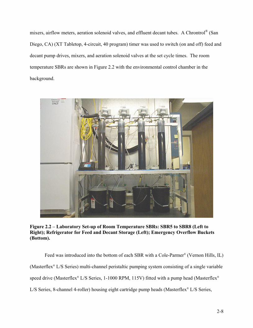
mixers, airflow meters, aeration solenoid valves, and effluent decant tubes. A Chrontrol® (San

Diego, CA) (XT Tabletop, 4-circuit, 40 program) timer was used to switch (on and off) feed and

decant pump drives, mixers, and aeration solenoid valves at the set cycle times. The room

temperature SBRs are shown in Figure 2.2 with the environmental control chamber in the

background.

Figure 2.2 – Laboratory Set-up of Room Temperature SBRs: SBR5 to SBR8 (Left to Right); Refrigerator for Feed and Decant Storage (Left); Emergency Overflow Buckets (Bottom).

Feed was introduced into the bottom of each SBR with a Cole-Parmer® (Vernon Hills, IL)

(Masterflex® L/S Series) multi-channel peristaltic pumping system consisting of a single variable

speed drive (Masterflex® L/S Series, 1-1000 RPM, 115V) fitted with a pump head (Masterflex®

L/S Series, 8-channel 4-roller) housing eight cartridge pump heads (Masterflex® L/S Series,

2-8

small). These pumps delivered feed at equal rates (within + 4% of the average) to each SBR.

Similarly, an identical Cole-Parmer® (Masterflex® L/S Series) multi-channel peristaltic pumping

system was used to decant effluent from the SBRs at equal rates (within + 4% of the average).

The liquid volume in the SBR was measured as a function of depth using a transparent ruler

mounted on the front each of the reactors and calibrated using tap water at the appropriate

operating temperature. Feed and decant flow rates were determined by measuring the depth

change per unit time. Feed was pumped from 15-liter high-density polyethylene (HDPE)

carboys and decant was collected in 9-liter HDPE carboys. Feed to and decant from the SBRs

were pumped through 1/8-inch polyethylene tubing. Tubing to and from the cold room was

insulated with 1-inch diameter foam tubing and both feed and decant containers were stored in a

Whirlpool® (Benton Harbor, MI) refrigerator-freezer (model EB22DKXFW01) maintained at

4oC.

A Cole-Parmer® (Stir-Pak® dual shaft, 1/25 horsepower, variable speed) mixer with two

(1.5-inch diameter) propellers was mounted on top of each SBR with the shaft offset at an angle

of approximately 4 degrees. The mixer speeds were set at 815+15 rpm. Compressed air was fed

through a filtered regulator and switched on and off with a 2-way Skinner Valve (New Britain,

CT) solenoid (7000 Series, 1/4-inch NPT). The air was fed through a 7/8-inch diameter spherical

Fisher Scientific (Pittsburgh, PA) fused alumina diffuser stone (model 11-139B, 60 micrometer

average pore size), one each mounted in the bottom of each SBR. Each SBR air line had a

dedicated flowmeter (Cole Parmer® 150 mm, aluminum frame, 46 mL/min maximum flow rate)

to measure the airflow rate and a Nupro® (Willoughby, OH) lift check valve (50 Series with 1/4-

inch Swagelock® fitting) to prevent wastewater from backfilling the air line.

2-9

A 3/8-inch ID stainless steel sludge wasting tube was used to drain the waste activated

sludge. It was fitted with a plug valve (Nupro® P6T Series, stainless steel, with 3/8-inch

Swagelock® fittings) mounted into the bottom of the SBR with a bore-through fitting to allow for

easy adjustment of the tube depth. The top of the tube was set at a depth of 7.4 cm from the

bottom of the SBR.

2.2.2 Experimental Conditions. The study was conducted in eight SBRs: one set of four

SBRs, receiving 0%, 3%, 6%, and 9% (v/v) feed concentrations of dyeing operation discharge

was operated at room temperature and another set receiving the same four concentrations was

operated in the cold room. The cold room SBRs were maintained at 7+2oC (including a defrost

cycle of 20 minutes three times per day) and the room temperature SBRs at 25+5oC for the

duration of the experiment and 22+2oC during stable reactor conditions. Table 2.1 summarizes

the experimental conditions for the eight SBRs.

Table 2.1: Feed Concentrations, Temperatures, and Solids Retention Time for the Eight Bench-Scale Sequencing Batch Reactors.

Cold Room SBRs: (Temperature = 7+2oC; Effective SRT = 28.1+0.5 days) SBR 1: 0% (v/v) Dyeing operation discharge (control) SBR 2: 3% (v/v) Dyeing operation discharge SBR 3: 6% (v/v) Dyeing operation discharge SBR 4: 9% (v/v) Dyeing operation discharge

Room Temperature SBRs (Temperature = 22+2oC; Effective SRT = 36.3+1.5 days) SBR 5: 0% (v/v) Dyeing operation discharge (control) SBR 6: 3% (v/v) Dyeing operation discharge SBR 7: 6% (v/v) Dyeing operation discharge SBR 8: 9% (v/v) Dyeing operation discharge

Reactors were seeded with sludge from a WWTP that nitrified but did not receive any

dye-bearing wastewater. No sludge was wasted during the first week of operation, to allow the

2-10

nitrifying bacteria to grow without being washed out and to acclimate to the dye. Sludge was

then wasted in small volumes at least once per day and often several times per day to reduce

shock to the biomass caused by intermittent wasting of large volumes of activated sludge. The

SRT was controlled by sludge wasting and was determined using the following equation:

SRT = (V)(MLSS)/[(Fw)(TSSw)+ (Fe)(TSSe)] (2.3)

Where

MLSS = mixed liquor suspended solids concentration in SBR,

V = volume of liquid in the SBR,

Fw = volumetric rate of sludge wasting,

TSSw = total suspended solids concentration of wasted sludge,

Fe = volumetric rate of effluent decant, and

TSSe = total suspended solids concentration in the effluent decant.

Although the suspended solids in the decant effluent can often be neglected when

determining the SRT, it is included in this expression due to the low concentration of solids in

the wasted sludge and the high concentration of solids in the effluent decant. The hydraulic

retention time (HRT) was determined from the following equation:

HRT = V/F (2.4)

where F is the volumetric flow rate of the feed to the SBR. Because the biochemical reactions

are assumed to occur only during the fill and reaction steps in the cycle (not during the settling,

decant, and idle steps), Grady et al. (1999) define the effective SRT (ESRT) and the effective

HRT (EHRT) as follows:

ESRT = (z)(SRT), and (2.5)

EHRT = (z)(HRT), (2.6)

2-11

where z is the fraction of the total cycle in which filling and reaction occurs; z was equal to 0.667

in this study. The SBRs in this study were operated at an ESRT of 28.1+0.5 days in the cold

room and 36.3+1.5 days at room temperature to provide sufficient time to maintain growth of the

nitrifying bacteria. The EHRT was 3.13+0.06 days in the cold room and 3.38+0.10 days at room

temperature.

Raw domestic sewage containing no dyeing operation discharge was collected from a lift

station feeding the WWTP. Discharge from the dyeing operation was collected from the facility

and included industrial wastewater from both the dumps and continuous rinse operations

(combined in a 1:1 ratio). The raw domestic sewage and dyeing operation discharge were

collected every four to thirteen days, transported, and mixed as needed to provide the dye-

bearing wastewater feed for the SBRs; all were stored at 4oC from collection until use.

The cycle time of each SBR was set at 6 hours and included a wastewater feed of 3 hours

(50% of the total cycle period) to match the average operating conditions of the WWTP. Grady

et al. (1999) suggests an aerobic fraction (AF) of between 0.5 and 0.8 to achieve optimum NH3

and NO3- removal, where AF equals “the fraction of the fill plus react period that is aerobic“.

The AF in this study was 0.625. Table 2.2 lists the length and description of each step within the

cycle.

The experiment was conducted for 62 days (approximately 2 SRTs), sufficient time to

allow all SBRs to achieve stability and show nitrification inhibition. Stability was verified by

examining effluent and mixed liquor concentrations to see if they approached asymptotic values.

All SBRs exhibited stable reactor conditions within 52 days of start-up.

2-12

Table 2.2: SBR Cycle Times with Description of Each Step in the Cycle. Step Duration Step Description

90 minutes static anoxic fill (raw sewage feed with no mixing or aeration) 90 minutes mixed aerated fill (raw sewage feed with mixing and aeration) 60 minutes aerated reaction (mixing with aeration) 5 minutes settling preparation (mixing with no aeration) 55 minutes settling (sludge settling with no mixing or aeration) 40 minutes decant (effluent decant with no mixing or aeration) 20 minutes idle time (no feed, decant, aeration, or mixing) 360 minutes total per cycle Fraction (Fill + React): z = (180 minutes fill + 60 minutes react)/360 total = 0.667 Aerobic Fraction: AF = (150 minutes aeration/240 minutes fill and react) = 0.625

2.2.3 Method of Analyses. Feed and effluent were analyzed for NH3, NO3-, NO2

-, total

Kjeldahl nitrogen (TKN), TSS, COD, BOD5, pH, alkalinity, and volatile suspended solids (VSS).

All nitrogen-containing compounds are expressed in terms of quantity of nitrogen (e.g. NH3-N

signifies the amount of nitrogen present as NH3). Because COD analyses provide more reliable,

reproducible, and faster results than BOD5 analyses, COD analyses were performed routinely.

Mixed liquor and settled sludge were analyzed for MLSS, mixed liquor volatile suspended solids

(MLVSS), and DO. All samples were stored at 4oC and, except for TKN, none were preserved

with sulfuric acid. Samples were analyzed within four days except for NH3 (analyzed within 24

hours), MLVSS and MLSS (analyzed within 24 hours), and TKN (analyzed within 3 weeks).

The analytical methods, frequency, and a brief description of each sample analysis are

summarized in Table 2.3. Temperatures were measured using thermometers submerged in the

room temperature SBRs and thermocouples submerged in the cold room SBRs and were

recorded weekly and during the oxygen uptake measurements.

Feed samples were collected for analysis after mixing. Decant tanks were emptied when

they became full and when newly mixed feed was added to the feed tanks; thus, SBR effluent

samples were composite samples of effluent decant for the entire period of decant collection

2-13

(between 4 and 8 days). Mixed liquor samples were collected by first scrubbing the walls of the

SBR with a nylon test tube brush to remove attached solids, purging the sludge wasting tube,

pouring the purge back into the SBR, and drawing a sample during aerated mixing.

Table 2.3: Description of Analytical Methods Used and Frequency of Sampling. Analysis Frequency Description Method [1] TKN Weekly Colorimetric, Digested EPA 351.2 NO3

-, NO2- Weekly Ion chromatography (IC) SM 4100-B

NH3-N Weekly Ammonia probe SM 4500-NH3F TSS, MLSS Weekly Filter, dry, weigh SM 2540-D BOD5 Monthly Incubation bottle SM 5210-B COD Weekly Open Reflux and titration SM 5220-B DO Monthly Oxygen probe SM 4500-OG pH Weekly pH probe SM 4500-H+B Alkalinity Monthly Titration SM 2320-B VSS, MLVSS Weekly Filter, ignite, weigh SM 2540-E [1] EPA: Environmental Protection Agency (1983); SM: Standard Methods for the Examination of Water and Wastewater (American Public Health Association et al., 1992).

Results from analysis of samples of the discharge collected from the dyeing operation

and of raw domestic sewage collected from the lift station are shown in Table 2.4. The dyeing

operation discharge and raw domestic sewage have similar characteristics, except for COD

which is more than three times higher in the dyeing operation discharge. These samples were

mixed to provide the dye-bearing wastewater feed to the SBRs during stable reactor conditions.

The concentration of AB1 in the feed to the SBRs throughout the duration of the study

varied due to the varying AB1 concentration in the samples collected from the industrial dyeing

operation. The AB1 concentration in the samples from the industrial discharge was determined

by measuring the peak absorbance (at 620 nm) using a Perkin Elmer (Lambda 2 Model) UV/VIS

Spectrometer. The AB1 concentrations over the course of the experiment are listed in Table 2.5.

2-14

Table 2.4: Concentration of Acid Black 1 in Dye-bearing Wastewater Feed During Study.

Wastewater Characteristic

Dyeing Operation Discharge

(grab sample)

Raw Domestic Sewage (lift station grab sample)

AB1 (mg/L) 810 0 BOD5 (mg/L) 87 100 COD (mg/L) 1,200 370 TKN (mg/L) 57 45 TSS (mg/L) 110 150

VSS/TSS (%) 85% 81%

Table 2.5: Concentration of Acid Black 1 in Dye-bearing Wastewater Feed During Study.

Acid Black 1 Dye Concentration in Reactor Feed (mg AB1/L)

SBR Number

Dyeing Discharge

(v/v)

18-24 daysafter

start-up

24-30 daysafter

start-up

30-52 days after

start-up

52-59 daysafter

start-up 1 & 5 0% (controls) 0 0 0 0 2 & 6 3% 15 9.3 24 5.8 3 & 7 6% 29 19 49 12 4 & 8 9% 44 28 73 18

Oxygen uptake was determined by measuring the DO concentration in a sample of mixed

liquor withdrawn at the end of the aerated mixing step and was determined at the same

temperature as the SBR. The sample was initially shaken in a closed bottle with a large

headspace bringing the DO concentration near saturation and then the change in DO

concentration was plotted over time. For exogenous samples, raw sewage containing no AB1

was added to the mixed liquor (raw sewage comprised 5% of the total volume) prior to shaking;

endogenous samples were not fed raw sewage.

2-15

2.3 RESULTS AND DISCUSSIONS

The performance of the reactors was examined over the duration of the study including at

stable reactor conditions attained at the end of the study (1.9 ESRTs). Although the

concentration varied throughout the study, during stable reactor conditions, the 3%, 6%, and 9%

(v/v) dyeing discharge in the feed corresponded to 24 mg AB1/L, 49 mg AB1/L, and 73 mg

AB1/L, respectively.

2.3.1 Analyses of Nitrogen Species. Figure 2.3 shows the concentrations of the various

forms of nitrogen (NH3-N, NO3--N, and TKN) in the feed and effluent during stable reactor

conditions as a function of AB1 concentration. Figure 2.3 indicates that there is no NH3 removal

and no substantial NO3- formation in the cold room SBRs fed dyeing operation discharge

compared to 99.9% NH3 removal, corresponding to an effluent NH3 concentration of 0.04 mg/L

NH3-N, achieved in the cold room control (fed no dye). The absence of NO2- (data not shown)

indicates that the first nitrification step (conversion of NH4+ to NO2

- by Nitrosomonas) is

inhibited by the dye-bearing wastewater. This agrees with the observation by Bitton (1999) that

many inhibitors are more toxic to Nitrosomonas than to Nitrobacter. He and Bishop (1994)

found that “ammonium oxidizers were more sensitive to AO7 than NO2- oxidizers”.

2.3.2 Ammonia Removal. Figure 2.3 shows that all room temperature SBRs achieved

greater than 96% ammonia removal. Figure 2.3 and TKN data (not shown) also indicate that

there was less than 20% denitrification in any of the reactors and this was probably due to the

high DO concentrations. Measuring the DO concentration throughout each step for an entire

cycle revealed that DO levels in the supernatant (above the sludge blanket) never dropped below

5 mg DO/L in any of the SBRs. Anoxic conditions only occurred during static fill and only

within the settled sludge blanket, which occupied a small fraction of the total SBR volume.

2-16

What should have been mixed anoxic fill (mixing without aeration during feed) was actually a

mixed aerobic fill.

0

10

20

30

40

0 24 49 73

Acid Black 1 Feed Concentration (mg AB1/L)

Nitr

ogen

Spe

cies

C

once

ntra

tion

(mg

N/L

)

Average Influent TKNAverage Influent AmmoniaEffluent Ammonia (7C)Effluent Nitrate (7C)Effluent Ammonia (22C)Effluent Nitrate (22C)

Figure 2.3 – Concentration Profile of Various Nitrogen Species in Cold Room (7oC) and at Room Temperature (22oC) at Stable Reactor Conditions.

Although all eight reactors initially achieved similar NH3 removals, over time, NH3

removal declined in the reactors fed dye. In the cold room SBRs, nitrification failed more

rapidly as the feed dye concentration increased. Figure 2.4 shows NH3 removal stopped at

approximately 38 days (1.4 ESRTs) after start-up for the 9% (v/v) dyeing discharge in the feed,

compared to 45 days (1.6 ESRTs) for 6% (v/v) discharge, and 52 days (1.9 ESRTs) for 3% (v/v)

discharge. In contrast, Figure 2.5 showed slight, but significant, nitrification inhibition in the

room temperature SBRs with 99.9%, 99.3%, 97.9%, and 97.0% NH3 removal for the room

temperature SBRs fed 0% (control), 3%, 6%, and 9% (v/v) dyeing operation discharge,

respectively. This corresponds to effluent NH3 concentrations of 0.03, 0.23, 0.69, and 1.0 mg/L

2-17

NH3-N for the room temperature SBRs fed 0% (control), 3%, 6%, and 9% (v/v) dyeing operation

discharge, respectively.

0%

20%

40%

60%

80%

100%

0 10 20 30 40 50 60Elapsed Time from Start-Up (days)

Am

mon

ia R

emov

al (%

)

0% Dye3% Dye6% Dye9% Dye

Figure 2.4 – Cold Room (7oC) Ammonia Removal During Experimental Period.

Daigger and Sadick (1998) similarly documented low temperature nitrification inhibition

by hydrocyanic acid (in incinerator flue-gas scrubber water) at a conventional activated sludge

WWTP. Cyanide reduced the nitrifier activity at all temperatures, but high effluent NH3

concentrations were only noticeable at low wastewater temperatures. The combined effects of

both cyanide and low temperature resulted in poor effluent quality data only during the colder

water period. Similarly, in this study, the combination of AB1 and low temperature resulted in

poor effluent quality only in the cold room reactors.

2-18

96%

97%

98%

99%

100%

0 10 20 30 40 50 60Elapsed Time from Start-Up (days)

Am

mon

ia R

emov

al (%

)

0% Dye3% Dye6% Dye9% Dye

Figure 2.5 – Room Temperature (22oC) Ammonia Removal During Experimental Period.

2.3.3 Additional Performance Characteristics. An increase in pH and the absence of

alkalinity consumption also indicated nitrification failure in the cold room SBRs fed dye-bearing

wastewater. At stable reactor conditions, the alkalinity decreased by approximately 230 mg

CaCO3/L in the control SBRs and by approximately 190 mg CaCO3/L in the room temperature

SBRs fed dye-bearing wastewater. This corresponds to approximately 6.6 mg HCO3- consumed

per mg NH3-N oxidized to NO3-N in the control SBRs and approximately 6.0 mg HCO3-

consumed per mg NH3-N oxidized to NO3-N in the room temperature SBRs fed dye-bearing

wastewater. This is close to the theoretical value determined by Bitton (1999) of 7.14 mg HCO3-

consumed per mg NH3-N oxidized to NO3-N. In the cold room SBRs fed dye-bearing

wastewater, the pH increased above 8.2 while the pH in the other SBRs remained below 7.5.

2-19

Figure 2.6 shows removal of organic nitrogen as a function of AB1 concentration.

Removal of organic nitrogen, which is biodegraded to ammonia by heterotrophs, decreases with

increasing dye concentration at both room temperature and in the cold room. Figure 2.7 shows

COD removal as a function of time. The dye-bearing wastewater reduced COD removal by as

much as 50% in the cold room SBRs. Less COD was removed (up to 20%) in the room

temperature SBRs (data not shown). Analysis of the soluble fractions of the feed and effluent

(data not shown) indicated lower soluble BOD5 and lower soluble COD removal in the cold

room SBR fed dye-bearing wastewater and lower soluble BOD5 removal in the room

temperature SBR fed dye-bearing wastewater. Only 35% of the soluble BOD5 was removed in

the cold room SRB fed 9% (v/v) dye-bearing wastewater and 95% of the soluble BOD5 was

removed in the room temperature SRB fed 9% (v/v) dye-bearing wastewater compared to greater

than 99% soluble BOD5 removal in the two control SBRs. Soluble COD removal was 45% in

the cold room SRB fed 9% (v/v) dye-bearing wastewater compared to approximately 60%

soluble COD removal in the room temperature SRB fed 9% (v/v) dye-bearing wastewater and

the two control SBRs.

Table 2.6 shows that effluent TSS was almost three times higher in the cold room SBRs

fed 6% and 9% dye and almost twice as high in the cold room SBR fed 3% dye when compared

to the cold room control SBR. Table 2.7 shows that both endogenous and exogenous oxygen

uptake by the activated sludge decreased (by 50% and 90%, respectively) in the cold room SBRs

fed 9% dyeing operation discharge. Neither endogenous nor exogenous oxygen uptake was

affected in the room temperature SBRs fed 9% dyeing operation discharge.

2-20

0%

20%

40%

60%

80%

100%

0 24 49 73Acid Black 1 Concentration (mg AB1/mL)

Org

anic

Nitr

ogen

Rem

oval

(%) Cold Room Organic Nitrogen Removal

Room Temperature Organic Nitrogen Removal

Figure 2.6 – Organic Nitrogen Removal in Cold Room (7oC) and Room Temperature (22oC) during Stable Reactor Conditions.

20%

40%

60%

80%

100%

0 10 20 30 40 50 60Elapsed Time from Start-Up (days)

CO

D R

emov

al (%

)

0% Dye3% Dye6% Dye9% Dye

Figure 2.7 – Cold Room (7oC) COD Removal During Experimental Period.

2-21

Table 2.6: Tabulation of Cold Room (7oC) Effluent TSS Concentration

SBR Number

Dyeing Discharge (v/v)

Effluent TSS (mg/L)

1 0% (control) 26 2 3% 46 3 6% 71 4 9% 68

Table 2.7: Tabulation of Oxygen Uptake Measurements of Activated Sludge

SBR Temperature

SBR Number

Dyeing Discharge

(v/v)

Endogenous Oxygen Uptake

(mg O2/g MLVSS-hr)

Exogenous Oxygen Uptake

(mg O2/g MLVSS-hr)1 0% (control) 1.7 11 Cold Room

(7oC) 4 9% 0.87 1.1 5 0% (control) 3.9 32 Room Temp.

(22oC) 8 9% 3.9 35

Furthermore, the quality of the activated sludge in all SBRs fed dye-bearing wastewater

deteriorated, as indicated by excessive foaming and by the presence of filamentous bacteria. The

most foaming occurred in the cold room SBRs fed 6% and 9% (v/v) dye-bearing wastewater.

According to Grady et al. (1999), foaming is primarily due to Nocordia and Microthrix

parvicella and a low food to microorganism (F/M) ratio can cause foaming with M. parvicella

present in the activated sludge. The F/M ratios in the SBRs that experienced foaming averaged

0.030 lb BOD5 applied per day/lb MLVSS and varied from 0.02 to 0.05 lb BOD5 applied per

day/lb MLVSS which is below the SBR design range of 0.05 to 0.30 lb BOD5 applied per day/lb

MLVSS specified by Tchobanoglous and Burton (1991). Foaming may also have been

aggravated by high air flow rates in each reactor. Microscopic examination (at 100X

magnification) shown in Figure 2.8 revealed excessive filamentous bacteria in the activated

sludge from the cold room SBR fed 9% (v/v) dye-bearing wastewater.

2-22

(a) (b) Figure 2.8 – (a) Activated Sludge from Sequencing Batch Reactor 1 Fed 0% (v/v) Dye-bearing Wastewater at 7oC; (b) Sequencing Batch Reactor 4 Fed 9% (v/v) Dye-bearing Wastewater at 7oC (Both Magnified 100X).

One concern was that the MLSS in all SBRs dropped to levels significantly lower than

those found in typical suspended growth treatment systems. The cold room SBRs had a MLSS

of 1,173+75 mg/L while the room temperature SBRs had a MLSS of 591+42 mg/L. However,

the non-inhibited SBRs were able to achieve pollutant removal even at these low MLSS.

Nitrification can occur at the low MLSS because nitrifiers grow slowly and produce little

biomass; “as a result, they may make a negligible contribution to MLSS concentration even

when they have a significant effect on process performance” (Grady et al., 1999). O’Neill et al.

(2000b) found “biomass growth in the activated sludge stage was limited by carbon source”

noting that the MLSS decreased from approximately 4,000 mg/L to 1,000 mg/L when the feed

concentration of starch was decreased from 3.8 mg/L to 1.9 mg/L; MLSS then increased after the

starch concentration was again increased to 3.8 mg/L. Grady et al. (1999) suggests nutrient

ratios for biological nitrogen removal of BOD5/NH3-N>4 and BOD5/TKN>2.5. In this study,

BOD5/NH3-N ranged from 2.2 to 4.0 and BOD5/TKN ranged from 1.8 to 3.6, indicating

2-23

insufficient carbon source. This is likely due to the low BOD5 concentration in the wastewater

collected from the lift station feeding the WWTP, which averaged 89+15 mg BOD5/L during this

study. This is less than 40% of the BOD5 concentration at the WWTP inlet, which averaged

228+53 mg BOD5/L.

During the final week of the study, the AB1 loading to the SBRs was reduced to see if the

activated sludge would recover. AB1 loading was decreased (by 75%) by decreasing the AB1

concentration in the feed (using only the less concentrated discharge from the continuous rinsing

operations) and by reducing the feed flow rate (by between 10% and 20%). Decreasing the AB1

loading to the cold room SBRs led to partial nitrification recovery indicated by NO3- production

of 11 mg NO3-/L, 1.0 mg NO3

-/L, and 0.10 mg NO3-/L in the SBRs fed 3%, 6%, and 9% (v/v)

dyeing operation discharge, respectively. There was also a slight improvement in COD removal.

Although NH3 removal did not improve, one week may not have been long enough for complete

recovery. Nitrification recovery (after reducing AB1 loading) would indicate that the nitrifiers

were inactivated instead of killed. Nitrification inhibition by AO7 was due to decreased nitrifier

activity, not nitrifier death (He and Bishop, 1994). AB1 and AO7 are both sulphonated azo dyes

having two common chemical structures: a naphthyl radical containing a hydroxyl functional

group adjacent to the azo bond and a phenyl radical unsubstituted adjacent to the azo bond.

Although the concentration of AB1 in the effluent was not measured, observations

indicated that the dye concentration was significantly higher in the feed than in the effluent. The

activated sludge in the reactors fed AB1 was also darker than in the control reactors indicating

that some AB1 may have been sorbed onto the activated sludge. Shaul et al. (1988) reported

only 2% to 6% of AB1 in feed sewage was sorbed onto the activated sludge with no apparent dye

biodegradation; however, this was for a continuous flow activated sludge system with the SRT

2-24

and HRT less than one tenth of those in this study, so more AB1 could have been sorbed onto the

sludge in this study.

2.3.4 Potential Solutions. While further investigation is required to determine the most

appropriate methods to reduce the impact of the dyeing operation discharge on the WWTP,

several options may be feasible. Treatment of the AB1 dye-bearing wastewater may be possible

by anaerobic digestion (possibly followed by aerobic treatment) or by addition of powdered

activated carbon to the aeration tanks at the WWTP. Another option is on-site pretreatment by

methods such as reduction followed by oxidation, coagulation and precipitation, lime

precipitation, or adsorption by activated carbon or other sorbents. Pollution prevention (i.e.

waste minimization, dye substitution, reuse, and/or equalization) is a potential strategy for

reducing the dye concentration in the wastewater and it may reduce dye concentration to a non-

inhibitory level. Eliminating dye-bearing wastewater discharge to the WWTP during the winter

(by hauling or storage) would also prevent cold weather nitrification failure at the WWTP.

Eventually, the dyeing industry relocated to another community. Eliminating this dye-

bearing wastewater discharge to the full-scale WWTP resulted in significantly improved

performance and brought the WWTP into compliance with regulatory discharge limits. Results

from this research and the full-scale WWTP demonstrate the complete nitrification failure at low

temperature due to dye-bearing wastewater which contained AB1, emphasizing the importance

of ascertaining inhibition at the lowest WWTP operating temperature.

2.4 CONCLUSIONS

1. Dye-bearing wastewater containing the azo dye AB1 at concentrations as low 24 mg AB1/L

inhibited nitrification after the reactors reached stable conditions. The combined effect of low

2-25

temperature and dye-bearing wastewater caused complete nitrification failure at 7oC within 2

ESRTs. Nitrification inhibition at 22oC was much less than at 7oC, but significant: 97.0% NH3

removal for 73 mg AB1/L compared to 99.9% for the 22oC control.

2. All reactors initially performed comparably, but over time, NH3 and COD removal declined

in all reactors fed dye. As the concentration of AB1 in the 7oC wastewater increased,

nitrification and COD removal failed earlier. For 24 mg AB1/L, 49 mg AB1/L, and 73 mg

AB1/L, the nitrification failure occurred in 52 days, 45 days, and 38 days after start-up,

respectively.

3. Decreasing the AB1 loading (by 77%) in the wastewater feed at 7oC led to partial nitrification

recovery within one week as indicated by significant NO3- production and a slight improvement

in COD removal; however, there was no corresponding increase in NH3 removal.

4. The presence of AB1-bearing wastewater led to additional deterioration in the activated

sludge process. COD removal decreased by as much as 50% at 7oC and by as much as 20% at

22oC; effluent TSS increased nearly three-fold at 7oC; both endogenous and exogenous oxygen

uptake decreased and foaming increased at 7oC.

5. The combined effects of both AB1 and low temperature resulted in poor effluent quality at

7oC, emphasizing the importance of ascertaining inhibition at the lowest WWTP operating

temperature.

2-26

2.5 ACKNOWLEDGEMENTS

2.5.1 Credits. This research was partially supported by Donohue & Associates (Sheboygan, WI)

with input provided by Ken Sedmack. During this project, Ron Martin, Jr. was supported as a

Michigan Technological University Graduate School Ph.D. and as a U.S. Department of

Education Graduate Assistantship in Areas of National Need (GAANN) Ph.D. fellow.

Christopher L. Wojick helped to design and construct the experimental equipment, Sue E.

Bunzendahl assisted with collection and analysis of samples, and David L. Perram provided

advice on analytical methods and technique (all of Michigan Technological University). Any

opinions, findings, conclusions, or recommendations expressed in this paper are those of the

authors and do not necessarily reflect the view of the supporting organizations.

2.5.2 Authors. Ron Martin, Jr. is enrolled in the Environmental Engineering Ph.D. program at

Michigan Technological University. C. Robert Baillod is a Professor and Chair in the

Department of Civil and Environmental Engineering and James R. Mihelcic is a Professor in the

Department of Civil and Environmental Engineering at Michigan Technological University.

Correspondence should be addressed to C. Robert Baillod, Department of Civil and

Environmental Engineering, Michigan Technological University, 1400 Townsend Drive,

Houghton, MI, 49931, email: baillod@mtu.edu.

2.6 REFERENCES

American Public Health Association; American Water Works Association; and Water

Environment Federation (1992) Standard Methods for the Examination of Water and

Wastewater. 18th Ed, edited Greenberg, A.E.; Clesceri, L.S.; and Eaton, A.D., Washington, D.C.

2-27

Åstrand, P.-O.; Ramanujam, P. S.; Hvilsted, S.; Bak, K.L.; and Sauer, S.P.A. (2000) Ab Initio

Calculation of the Electronic Spectrum of Azobenzene Dyes and Its Impact on the Design of

Optical Data Storage Materials. J. Am. Chem. Soc., 122 (14), 3482 -3487.

Bitton, G. (1999) Wastewater Microbiology. 2nd Ed., Wiley-Liss (A John Wiley & Sons, Inc.

Publication), New York.

Brown, D., and Hamburger, B. (1987) The Degradation of Dyestuffs: Part III - Investigation of

Their Ultimate Degradability. Chemosphere, 16(7), 1539-1553.

Brown, D.; Hitz, H.R.; and Schafer, L. (1981) The Assessment of the Possible Inhibitory Effect

of Dye-stuffs on Aerobic Wastewater Bacteria Experience with a Screening Test. Chemosphere,

10(3), 245-261.

Burg, A.W., and Charest, M. C. (1980) Azo Dyes: Evaluation of Data Relevant to Human Health

and Environmental Safety. Report C-82875 to the Dyes Environmental and Toxicology

Organization, Arthur D. Little, Inc. and the Ecological and Toxicological Association of the

Dyestuffs Manufacturing Industry (ETAD), Basel, Switzerland.

Daigger, G.T., and Sadick, T.E. (1998) Evaluation of Methods to Detect and Control

Nitrification Inhibition with Specific Application to Incinerator Flue-Gas Scrubber Water. Water

Env. Res., 70(7), 1246-1257.

2-28

Environmental Protection Agency (1983) Methods of Chemical Analysis of Water and Wastes.

US EPA/600/4-79-020, US Environmental Protection Agency, Environmental Monitoring

Systems Laboratory (EMSL), Cincinnati, OH.

Fu, Y.C.; Jiang, H.; and Bishop, P. (1994) An Inhibition Study of The Effect of Azo Dyes on

Bioactivity of Biofilms. Wat. Sci. Tech., ASCE, 29(7), 365-372.

Furukawa, K.; Kuroki, S.; and Nakaoka, M. (1999) Biodegradation Azo Dyes Under Photo-

dependent Anoxic Conditions. Proc. Water Environ. Fed. 72nd Annu. Conf. Exposition [CD-

ROM], New Orleans, La.

Grady, C.P.L. Jr.; Daigger, G.T.; and Lim, H.C. (1999) Biological Wastewater Treatment, 2nd

Ed., Marcel Dekker, Inc., New York.

Harmer, C., and Bishop, P. (1992) Transformation of Azo Dye AO-7on by Wastewater Biofilms.

Wat. Sci. Tech., 26(3-4), 627-636.

He, Y., and Bishop, P.L. (1994) Effect of Acid Orange 7 on Nitrification Process. J. Envir.

Eng., 120(1), 108-121.

McCurdy, M.W.; Boardman, G.D.; Michelsen, D.L.; and Woodby, B.M. (1992) Chemical

Reduction and Oxidation Combined with Biodegradation for the Treatment of a Textile Dye

Wastewater. 46th Ind. Waste Conf. Proc., Conference Date 1991, 46, 229-234.

2-29

Nigam, P.; Banat, I.M.; Singh, D.; and Marchant, R. (1996) Microbial Process for the

Decolorization of Textile Effluent Containing Azo, Diazo and Reactive Dyes. Process

Biochemistry, 31(5), 435-442.

O’Neill, C.; Hawkes, F.R.; Hawkes, D.L.; Esteves, S.; and Wilcox, S.J. (2000b) Anaerobic-

Aerobic Biotreatment of Simulated Textile Effluent Containing Varied Ratios of Starch and Azo

Dye. Wat. Res., 34(8), 2355-2361.

O’Neill, C.; Lopez, A.; Esteves, S.; Hawkes, F.R.; Hawkes, D.L.; and Wilcox, S. (2000a) Azo-

Dye Degradation in and Anaerobic-Aerobic Treatment System Operating on Simulated Textile

Effluent. Appl. Microbiol. Biotechnol., 53(2), 249-254.

Razo-Flores, E.; Luijten, M.; Donlon, B.; Lettinga, G.; and Field, J. (1997) Complete

Biodegradation of the Azo Dye Azodisalicylate Under Anaerobic Conditions. Environ. Sci.

Technol., 31(7), 2098-2103.

Shaul, G.M.; Dempsey, C.R.; and Dostal, K.A (1988) Fate of Water Soluble Azo Dyes in the

Activated Sludge Process. US EPA/600/S2-88/030, US Environmental Protection Agency, Water

Engineering Research Laboratory, Cincinnati, OH.

Tchobanoglous, G., and Burton, F.L. (1991) Wastewater Engineering Treatment, Disposal, and

Reuse. 3rd Ed. Metcalf & Eddy, Inc. Published by Irwin/McGraw-Hill (a division of the

McGraw-Hill Companies. Boston, MA.

2-30

2-31

Tong, A., and Young, R. A. (1974) An Investigation into the Pretreatment and Effect of an

Industrial Waste Water Derived from the Manufacture of Azo Dyes upon the Activated-Sludge

Process. Water Pollut. Control, 73(5), 584-588.

Vandevivere, P.C.; Bianchi, R.; and Verstraete, W. (1998) Review: Treatment and Reuse of

Wastewater from the Textile Wet-Processing Industry: Review of Emerging Technologies. J.

Chem. Technol. Biotechnol., 72(4), 289-302.

Zaoyan, Y.; Ke, S.; Guangliang, S.; Fan, Y.; Jinshan, D.; and Huanian, M. (1992) Anaerobic-

Aerobic Treatment of a Dye Wastewater by Combination of RBC with Activated Sludge. Wat.

Sci. Tech., 26(9-11), 2093-2096.

CHAPTER 3 OPTIMIZATION OF BIOFILTRATION FOR ODOR CONTROL: MODEL CALIBRATION, VALIDATION, AND APPLICATIONS* ABSTRACT

A dynamic model that describes the biofiltration process for hydrogen sulfide removal from

wastewater treatment plant air emissions was calibrated and validated using pilot- and full-scale

biofilter data obtained from the Cedar Rapids (Iowa) Water Pollution Control Facilities. After

calibration, the model was found to predict the dynamic effluent concentrations of the pilot- and

full-scale biofilters very well, with the measured data falling within 58 to 80% of the model

output values. In addition, the model predicted the trend of the field data even under field

conditions of changing input concentration and at effluent concentrations below 1 ppm by

volume. The model demonstrated that increasing gas residence time and temperature and

decreasing influent concentration decreases effluent concentration. In addition, model

simulations showed that a longer residence time is required to treat dynamic loading increases,

indicating that biofilter design should account for the maximum influent concentration. These

results can be used to assist in the design and operation of biofilters for control of odorous and

hazardous air emissions.

KEYWORDS: Biofilter, biofilm, biological treatment, hydrogen sulfide, model calibration and

validation, odor, organic sulfur compounds, pilot plant, VOC, wastewater.

* Reprinted with permission from Martin Jr., R. W.; Li, H.; Mihelcic, J. R.; Crittenden, J. C.; Lueking, D. R.; Hatch, C. R.; Ball, P. (2002) Optimization of Biofiltration for Odor Control: Model Calibration, Validation, and Applications. Water Environ. Res., 74, 17. Copyright 2002 Water Environment Federation, Alexandria, VA.

3-1

3.1 INTRODUCTION

In a companion study (Li et al., 2002) a dynamic model that can simulate the

performance of a biofilter used to control odorous hydrogen sulfide (H2S) emissions was

developed and verified, and a parameter sensitivity analysis was conducted. The model, which

has been packaged as a user-friendly software program called BiofilterTM (Michigan

Technological University, Houghton, Michigan), provides a tool for the design and optimization

of biofilters used for controlling odorous air emissions. The objectives of this study are to present

the calibration and validation of the biofilter model using pilot- and full-scale data from the

Cedar Rapids (Iowa) Water Pollution Control Facilities (WPCF) and then demonstrate some of

the model’s practical applications. These practical applications include the influence that gas

residence time, influent concentration, temperature, and dynamic loading have on biofilter

performance and design.

Although a much less complex biofiltration model has been compared to laboratory-scale

experimental data for H2S (McNevin et al. 1999), other laboratory studies have been directed at a

wide variety of organic chemicals such as methyl ethyl ketone and methyl isobutyl ketone

(Deshusses et al., 1995), benzene and toluene (Zarook et al., 1997), and volatile organic

compounds (VOCs) (Amanullah, 1999). Although it is easy to control conditions such as

temperature and loading in the laboratory, these conditions are more difficult to control in the

field. In addition, the operational and performance problems of full-scale biofilters are different

from those encountered in laboratory studies (Webster et al., 1999). Therefore, model parameters

obtained from laboratory-scale data may not predict biofilter performance in the field. For this

reason, pilot- and full-scale data from the Cedar Rapids WPCF were used to calibrate and

validate the model in this study. Although Comas et al. (1999) conducted a pilot study with a

3-2

bioscrubber to support a modeling effort, instead of changing the model parameters to fit the data

they developed a correlation between the simulated effluent and the experimental effluent that is

not easily used or compared by other researchers.

Finally, a major difference in the literature describing several types of biofilter designs

for H2S removal is the type of packing medium employed. For example, van Langenhove et al.

(1986) used wood bark, Hirai et al. (1990) used peat, Yang and Allen (1994) used compost,

Chung et al. (1996) used calcium-alginate pellets, Morton and Caballero (1996) used lava rock,

and Wani et al. (1998) used various mixtures of compost, perlite, and hog fuel. The packing

material used by the Cedar Rapids WPCF is lava rock. Accordingly, this paper also discusses

issues related to the selection of the packing material and provides insight on some potentially

beneficial properties of lava rock.

3.2 MATERIALS AND METHODS

3.2.1 Background. The Cedar Rapids WPCF receives an average flow of approximately

2.0 m3/s (45 MGD), have a design average flow of 2.5 m3/s (56 MGD), and a design peak flow

of 4.8 m3/s (110 MGD). Approximately 70% of the flow contribution is from industrial

discharges resulting in high influent concentrations of BOD (>500 mg/L) and sulfate (250 to 400

mg/L).

Four roughing filters reduce the high BOD and chemical oxygen demand (COD) loading

to the carbonaceous activated sludge (CAS) system, thus decreasing demand for the pure oxygen

activated sludge aeration. A 1990 odor study by the Cedar Rapids WPCF indicated that 90% of

odor emissions originated from the roughing filters, with additional odor emissions originating

3-3

from three dissolved air flotation (DAF) thickeners, three primary clarifiers, and a Parshall flume

that measures inlet flow.

Lava Rock Packing Material

RoughingFilter 4

Intermittent RinseWaterFeed

RinseWater

Effluent

Make-upAir

IntermittentRinseWaterFeed

RinseWater

Effluent

TreatedEffluent

Air

H2S Sampling Port

H2S Meter (Conspec & API)

Lava Rock Packing Material

Full-Scale Biofilter

TreatedEffluent

Air

H2S Meter(MSA)

RoughingFilter 1

Pilot-ScaleBiofilter

H2S Meter(MSA)

3 Primary Clarifiers

Parshall Flume

3 DAF Thickeners

Make-upAir

Pilot-Scale Biofilter

Make-upAir

Figure 3.1Process Flow Diagram for Pilot-Scale Biofilter (Located within Dashed Area and Used for Model Calibration and Validation) and Full-Scale Biofilter 1 (Used for Model Validation) at Cedar Rapids WPCF. Air Streams are Shown as Solid Lines and Intermittent Rinse Water Streams are Shown as Dashed Lines.

3-4

Bacteria in the roughing filters reduce the sulfate to sulfide under the anaerobic

conditions caused by high BOD loading. Additionally, any sulfide dissolved in the wastewater

entering the roughing filters is stripped into the air as it is agitated while passing over the

packing material. Although H2S is the odorous contaminant present at the highest concentration,

methyl mercaptan, carbonyl sulfide, ethyl mercaptan, dimethyl sulfide, carbon disulfide, and

dimethyl disulfide have also been detected. While the model used in this study could be applied

to the removal of organic reduced sulfur compounds and VOCs, the focus of this study was on

H2S removal.

3.2.2 Biofilters and Packing Medium. In 1998, Cedar Rapids WPCF began operation of

two, parallel, full-scale biofilters. Each biofilter is 21.6-m (71-ft) long by 11-m (36-ft) wide.

Biofilter 1 treats odorous air from roughing filters 1 and 4 while biofilter 2 treats odorous air

from roughing filters 2 and 3. Each roughing filter has a blower on the air effluent that feeds the

odorous air to the biofilters’ upflow and draws ambient make-up air into the roughing filters.

Roughing filter 1 also draws odorous air from the DAF thickeners (accounting for 45% of the

total make-up air flow to roughing filter 1), primary clarifiers (14%), and Parshall flume (4.5%).

Each biofilter has an exhaust stack with a blower that discharges effluent air to the atmosphere.

Figure 3.1 shows the process flow diagram for biofilter 1 as well as the pilot-scale

biofilter and also includes the location of sampling points used for calibration and validation of

the model. The pilot-scale biofilter consisted of a 0.608-m (2.00-ft) inside diameter vertical

fiberglass cylinder that was covered with insulation. An electric blower (IPF, Inc., Wakefield,

Massachusetts, model CDD-180, 0.2 m3/s [400 cfm] and 1,725 rpm) pulled odorous air from

roughing filter 1 effluent and fed it to the bottom of the pilot biofilter through a 15-cm (6-in.)

polyvinyl chloride (PVC) feed pipe that entered at the side of the biofilter column. Exhaust air

3-5

exited through a 10-cm (4 in.) diameter by 15-cm (6-in.) long cylindrical stack that was offset 15

cm (6 in.) from the axial center on top of the column, with 0.9 m (3 ft) of headspace above the

packing medium.

Both the full-scale biofilters and the pilot-scale biofilter were packed with lava rock to a

depth of 1.83 m (6 ft). The lava rock had an average radius of 1.20 cm and a sphericity of 0.5 and

the bed porosity was determined to be 0.40. In both full-scale biofilters and the pilot biofilter, a

PVC peg board, with 0.64-cm (0.25-in) holes that were 7.6 cm (3 in) apart, supported the lava

rock above the gas feed and provided uniform air distribution through the beds.

To provide moisture and nutrients for the microorganisms and to prevent excess sulfate

accumulation, which has been shown to decrease removal efficiency (Yang and Allen, 1994),

CAS clarified effluent was sprayed on top of the lava rock beds via spray nozzles for 5 minutes

every hour. The continuous air stream (fed upward from the bottom of the bed) and the

intermittent rinse water flowed countercurrent, with spent rinse water collected in, and

overflowing from, a sump located below the biofilters. The pilot biofilter was operated using an

air residence time and rinse water feed flow rate (per bed volume) set approximately equal to that

of the full-scale biofilters at the time of the pilot study.

3.2.3 H2S Data Collection. The pilot study, initiated on January 17, 2000, collected two

sets of data: the first in January and the second in March. Feed influent to the full-scale biofilters

was measured by an individual Mine Safety Appliances (MSA) Company (Pittsburgh,

Pennsylvania) odor monitoring system consisting of an H2S meter dedicated to each of the four

roughing filter effluent air pipes. The 4- to 20-mA output signal from each MSA meter was

continuously recorded. The influent H2S concentration to the pilot biofilter was measured using

the MSA meter on roughing filter 1. Each MSA meter was calibrated monthly by WPCF staff.

3-6

The MSA meter was crosschecked twice with a Conspec hydrogen sulfide monitor (series

P2065-1 with a 0- to 80-ppm by volume [ppmv] concentration range) (Conspec Controls, Inc.,

Charleroi, Pennsylvania) when the pilot feed H2S concentration was within the working range of

the Conspec meter. The effluent from the full-scale biofilter was measured with a Jerome 631-X

hydrogen sulfide analyzer (Arizona Instrument Corp., Phoenix, Arizona).

Several meters were used to measure the effluent H2S concentrations from the pilot-scale

biofilter. When the effluent H2S concentration was high (corresponding to the first data

collection in January), the effluent H2S concentration was recorded from the digital readout of

the Conspec meter. During the second data collection in March, the 4- to 20-mA output signal

from the Conspec meter was continuously recorded during the period from 11 p.m. on March 7,

2000 to 11 a.m. on March 10, 2000. The Conspec meter was calibrated (according to the

manufacturer’s specifications) at the beginning of both data collections. Both the digital readout

and the (4- to 20-mA) signal output were checked with standards (carbon filtered air for zero and

1-, 5-, and 40-ppmv standard H2S gas), once during and once at the end of both data collection

periods. An Advanced Pollution Instrumentation (API) (San Diego California) hydrogen sulfide

analyzer (model 101A with a 0- to 20-ppmv concentration range) was used to measure the

effluent H2S concentration during the low-concentration period (from 1 p.m. on March 10, 2000,

to 6:30 p.m. on March 14, 2000). The 4- to 20-mA output signal from the API meter was

continuously recorded. The inlet to the API meter was fitted with a stock SO2 scrubber (SO2 will

result in a high H2S reading) and a hydrophobic filter (Whatman Puradisc 25TF, Whatman, Inc.,

Clifton, New Jersey) to protect the meter from moisture. The API meter was calibrated

(according to the manufacturer’s specifications) at the beginning of use and the (4- to 20-mA)

3-7

output signal was checked with standards (carbon filtered air for zero and 1- and 5-ppmv

standard H2S gas) once during and once at the end of this period.

All H2S meter sampling of effluent air was conduced from the exhaust stack on the top of

the pilot biofilter column. For the continuous, 4- to 20-mA) signal output readings, an API

(Model 101A) external vacuum pump was used to continuously pull effluent air samples through

a 0.6-cm (0.25-in) i.d. polyethylene tubing running from the exhaust stack to a heated

maintenance building. A water trap on top of the pilot biofilter column and a drying tube

(containing Drierite [anhydrous calcium sulfate]) located in the building were used to remove

moisture from the air sample.

3.2.4 Additional Data Collection. The odorous airflow to the pilot-scale biofilter was

measured (as velocity) using both hot wire (series 471 Dwyer Instruments, Inc., Michigan City,

Indiana and standard model Extech Instruments, Corp., Waltham, Massachusetts) and

mechanical vane-type (model DA40V, Pacer Industries, Chippewa Falls, Wisconsin) hand-held

digital anemometers. The pilot biofilter temperature, which varied in both the axial and radial

directions of the biofilter bed, was measured at sample holes at various column depths by

inserting the metal stem of a digital thermometer approximately 13 cm (5 in.) into the biofilter,

toward the column center. The temperature of the odorous feed air and the rinse water feed were

also manually recorded. The rinse water effluent temperature and pH were measured in the sump

with a Rosemont Analytical, Inc. (Irvine, California) pH/oxidation reduction potential meter

(model 54, with a model 396P sensor). The rinse water flow was measured with a King

Instrument Company (Garden Grove, California) 1.9- to 18.9-L/min (0.5- to 5.0-gpm) inline

flow meter and maintained at 3.8 L/min (1.0 gpm) during the 5-minute rinse cycle. An Isco, Inc.

(Lincoln, Nebraska) model 2910 sampler was used to collect composite samples for pH and

3-8

sulfate analysis of feed and effluent (from the sump) rinse water. Measurements (not reported

here) were also made of the BOD, total Kjeldahl nitrogen, total phosphate, conductivity,

alkalinity, and total suspended solids in the rinse water influent and effluent.

3.2.5 Calibration and Validation Periods. The most suitable data set for model

calibration would be from an extended period of relatively constant feed H2S concentration and

biofilter bed temperature. Such an ideal data set was not available because of the diurnal

variation of BOD and sulfate loading to the roughing filters as well as the column temperature

fluctuation. However, measured data from the pilot-scale biofilter in March (starting at 12:30

a.m. on March 8, 2000 and ending at 7:30 a.m. on March 14, 2000) with a relatively constant

feed H2S concentration and a relatively constant column temperature was determined to be

appropriate for the model calibration period.

For the model validation period, measured data from the pilot-scale biofilter obtained in

January were used (starting at 2:30 p.m. on January 17, 2000 and ending at 1:30 p.m. on January

27, 2000). An additional model validation data set was obtained using measured data from the

full-scale biofilter for a 26-day period (starting at noon on October 9, 1998 and ending at 1:30

p.m. on November 3, 1998). Unlike the continuously measured H2S concentration data for the

pilot-scale study, the full-scale data consisted of between one and three individual measurements

per day.

3.2.6 Data Input for the Model. Hourly average feed and hourly average effluent H2S

concentrations were used for model input values and for data used for comparison with the pilot-

scale model simulation outputs, respectively. An average flow of 1.7 m3/min (60 cfm) was used

for the pilot-scale model input calibration and validation. This flow rate corresponded to a

3-9

retention time of 7.5 seconds. A constant airflow rate of 1,246 m3/min (44,000 cfm) was used for

the full-scale model input validation, corresponding to a retention time of 8.4 seconds.

The column temperature varied from 17 to 27oC over the course of the pilot calibration

and from 8 to 16oC over the course of the pilot validation. At any time, the bed temperature was

relatively uniform throughout the various bed depths. Although the bed temperature varied,

average bed temperatures of 20 and 11.5oC were used for the calibration and validation periods,

respectively, because the model software currently only allows a single constant input of

temperature-dependent variables.

During and shortly after the 5-min rinse cycle, unexpectedly high effluent H2S

concentrations were measured in the pilot biofilter. This was most likely caused by two

phenomena. First, a companion study (Li et al., 2002) showed that the formation of a water layer

during the rinse cycle would inhibit mass transfer to the biofilm. Secondly, the influent rinse

water sprayed onto the biofilter bed contained dissolved H2S, which may have been stripped

from the solution after passing through the spray nozzle. H2S stripping was confirmed by

shaking a sample bottle of unused rinse water feed and measuring high H2S concentrations (up to

36 ppmv) in the sample bottle headspace. Because this flashing occurred in the headspace

directly above the lava rock, it never came into contact with the biofilm; thus, effluent data

obtained during the rinse cycle were excluded. Exclusion of these data also allowed the authors

to maintain the assumption that the BiofilterTM two-phase model would describe the biofilter

conditions.

3.2.7 Model Calibration and Validation. The BiofilterTM two-phase (solid-gas) model

was used for this study. Because the actual water content in the biofilters was small (except

during the 5-minute rinse cycle when the data were excluded), the two-phase model would

3-10

describe the biofilter conditions for most of the time (Hautakangas et al., 1999 and Li et al.,

2002). The model calibration was achieved by minimizing the value of an objective function and

by minimizing the sum of the residuals. The objective function used for the model calibration

criteria was:

2

data,i model,i

1 data,i

1OF1

n

i

C Cn C=

−= −

∑ (3.1)

Where

OF = objective function,

n = number of measured data points,

Cdata = measured effluent concentration, and

Cmodel = model output effluent concentration.

It was not possible to obtain low values for the objective function because a small error

within the low concentration range (< 1.0 ppmv) resulted in large values of the OF. However, it

was possible to minimize the sum of the residuals close to zero so that the errors were randomly

distributed. The sum of the residuals is defined as follows:

data,i model,i

1 model,i

n

i

C CC=

−∑ (3.2)

According to the model sensitivity analysis (Li et al., 2002), the effluent concentration

was sensitive to the biofilm diffusivity and the biological kinetic parameters. The values of these

parameters were adjusted within the corresponding variation ranges (Li et al., 2002) to minimize

the value of the objective function and to obtain a sum of the residuals close to zero for the

calibration period.

For modeling, the biofilm was assumed to be homogenous and a thickness of the biofilm

was chosen to ensure that all of the active biofilm was considered. This assumed thickness is not

3-11

the actual biofilm thickness, per se, because the actual biofilm contains active and inactive

biomass and the substrate concentration and system dynamics determine both the active biofilm

thickness and the active biomass concentration gradient in the biofilm as function of time. This

assumption may have underestimated the mass transport from the bulk phase to the biofilm.

Gjaltema et al. (1994) pointed out that biofilm inhomogeneity can increase the contact area

between the bulk phase and the biofilm, and a rough surface can also improve external and

internal mass transfer. As a result, the biofilm inhomogeneity may have significantly influenced

the overall rate of removal, and this is reflected in the model parameters that were determined

from model calibration.

The biological, physical, and mass transfer model parameters that were determined for

the calibration period at 20oC were corrected to the actual biofilter temperature for the validation

periods. The maximum specific biomass growth rate (µmax) was corrected using the Arrhenius

relationship with coefficients reported by Shinabe et al. (1995). Because there is no general

consensus on the temperature effect on the Monod half-saturation constant (Ks), it was assumed

to be constant over the temperature range in this study (Grady et. al., 1999). The Henry’s

constant (H) was corrected for temperature with a van’t Hoff-type equation using the

temperature correction factors provided by Montgomery (1985). The diffusivity of H2S in the

biofilm (Db) was adjusted to fit the data during the calibration. Because Db was assumed to be

directly proportional to the diffusivity of H2S in water (Fan et. al., 1990), it was corrected for

temperature using the Hayduk and Laudie (1974) correlation. Although the gas-biofilm mass

transfer coefficient was expected to change with temperature, the change was neglected because

the model output was not found to be sensitive to the gas-biofilm mass transfer coefficient (Li et

al., 2002) over the experimental temperature range used in this study.

3-12

3.3 RESULTS AND DISCUSSION

3.3.1 Model Calibration. When the initial default parameter values were used for the

calibration period, the model predicted much higher effluent concentrations than the actual

effluent concentrations. Db and µmax were adjusted to maintain the sum of the residuals close to

zero. In addition, the biological parameters, KS and Y (biomass yield coefficient), were optimized

by minimizing the value of the objective function. The initial default parameter values and those

for the final calibration are listed in Table 3.1.

Table 3.1Values of Parameters Used for Model Calibration and Validation.

Parameter Symbol Default Values

Pilot-Scale Calibration

Values (20°C)

Pilot-Scale Validation

Values (11.5°C)

Full-Scale Validation

Values (25°C)

Biofilm diffusivity Db (cm2/s) 3.69×10-6 4.65×10-6 3.60×10-6 5.30×10-6

Maximum specific biomass growth

rate µmax (1/hr) 0.20 0.28 0.066 0.58

Biomass yield coefficient Y (g cells/mol S) 5.6 3.8 3.8 3.8

Monod half saturation coefficient

KS (µmol/L) 4.8 3.5 3.5 3.5

Henry’s Constant H (dimensionless) 0.379 0.379 0.313 0.420

Figure 3.2 compares the effluent H2S pilot-scale data to the model simulations for the

calibration period. Figure 3.2 also shows the influent H2S concentration initially increasing from

50 to 250 ppmv, and then varying from approximately 100 to 200 ppmv. In this “best fit” case,

the objective function was minimized to 0.42, signifying that approximately two-thirds of the

3-13

measured data fell within 42% of the model output values (assuming a Gaussian distribution).

The objective function of 0.42 was deemed acceptable considering that most of the measured

effluent concentrations were below 1 ppmv and a small error within this low concentration range

(< 1 ppmv) resulted in large values of the objective function. Visual inspection of the plotted

residuals (not shown) showed a random distribution and the mean sum of the residuals was

0.014.

0.0

0.5

1.0

1.5

2.0

2.5

3.0

3/7/00 3/8/00 3/9/00 3/10/00 3/11/00 3/12/00 3/13/00 3/14/00 3/15/00

Efflu

ent H

2S C

once

ntra

tion

(ppm

v)

0

50

100

150

200

250

300

Influ

ent H

2S C

once

ntra

tion

(ppm

v)

Model Simulation EffluentMeasured EffluentMeasured Influent

Date

Figure 3.2Model Simulated Effluent Concentration Compared to the Measured Effluent for the Calibration Period.

Analysis at the end of the model calibration period of one grab sample collected from the

influent and effluent air indicated the following removal of other odor causing chemicals: 98%

3-14

removal of 3.13 ppmv methyl mercaptan, 98% removal of 0.12 ppmv dimethyl disulfide, 58%

removal of 1.25 ppmv carbonyl sulfide, and 38% removal of 0.63 ppmv dimethyl sulfide.

Analysis of several 24-hour composite rinse water samples collected during the

calibration period indicated that the rinse water pH decreased from the top of the column to the

bottom. The average rinse water pH was 7.2 in the feed and 1.9 in the sump effluent. The

average sulfate concentration in the rinse water increased from approximately 500 mg/L in the

feed to 3,000 mg/L in the sump effluent, indicating oxidation of H2S and removal of the

accumulated sulfate. Removal of the oxidation product, sulfate, was important because Yang and

Allen (1994) found that sulfur accumulation above 40 mg S/g bed packing (dry weight) inhibited

sulfide oxidation for various compost packing materials.

3.3.2 Model Validation. Figure 3.3 shows the model-predicted effluent concentration

and actual data for the pilot-plant validation period. These data were obtained at a lower average

temperature (11.5oC) than the pilot-scale calibration period (20oC). Accordingly, certain model

input parameters (Db, µmax, and H) were adjusted for the lower temperature (Table 1). The

objective function was 0.61 and the mean sum of the residuals was -0.016. One interesting

feature was that the model predicted the decrease in effluent H2S concentration that was

observed during start up of the pilot-scale study.

When the model was initially validated to the full-scale validation data set, the measured

effluent H2S concentrations (approximately 0.1-1.4 ppmv) from the full-scale biofilter were

slightly higher than the model predictions (approximately 0.1-0.5 ppmv). Several explanations

were examined to explain this occurrence. One possible explanation for the slightly lower

concentration predicted by the model is that there may have been air-flow channeling in the full-

scale biofilter that would be far more prevalent in a large rectangular bed than in the small

3-15

cylindrical column used for the pilot study. Running the model assuming channeling (by

decreasing the bed volume by 40%) resulted in a model output that fit the measured effluent

concentrations (results not shown). However, smoke tests indicated that there was no significant

air channeling occurring in the field.

0

10

20

30

40

50

60

70

80

1/17/00 1/19/00 1/21/00 1/23/00 1/25/00 1/27/00 1/29/00

Efflu

ent H

2S C

once

ntra

tion

(ppm

v) Model Simulation Effluent

Measured Effluent

Date

Figure 3.3Model Simulated Effluent Concentration Compared to the Measured Effluent for the Pilot-Scale Validation Period.

Another explanation for the lower model predictions is the presence of small “dead

zones” of activity in the biofilter bed having either poor removal or no removal at all. This

phenomenon has been observed by Webster et al. (1999). Reasons for these “dead zones” could

be poor microbial growth or microbial inhibition caused by nonuniform rinse water coverage or

nonoptimal pH. Accordingly, dead zones were considered by assuming that a specified fraction

of the biofilter bed (a depth cross-section) provided no removal and the remainder of the bed

3-16

achieved the removal predicted by the model. The resulting effluent was calculated using a

volumetric weighted-average of the effluent of the active and inactive bed fractions.

Figure 3.4 shows the actual measured data compared to the model output for an assumed

1.0 % inactive bed fraction. The fit to the low concentration effluent data visually appears to be

good, and the objective function was 0.80. A plot of the residuals showed they were randomly

distributed (figure not shown) and the mean sum of the residuals was -0.0067. While this does

not conclusively prove there were dead zones within the full-scale biofilter, it does demonstrate

the importance of ensuring that design and operation of biofilters result in a system that

maximizes the biologically active zones. This may be more significant in biofilters that use

organic media (e.g., compost or wood chips) that are less uniform and more prone to drying than

the lava rock employed at the Cedar Rapids WPCF.

0.0

0.5

1.0

1.5

2.0

2.5

3.0

10/9/98 10/13/98 10/17/98 10/21/98 10/25/98 10/29/98 11/2/98

Efflu

ent H

2S C

once

ntra

tion

(ppm

v) Measured Effluent

Model Simulation Effluent

Date

Figure 3.4Model Simulated Effluent Concentration Compared to the Measured Effluent for the Full-Scale Validation Period Assuming 1.0% of the Bed Is Inactive.

3-17

Figure 3.4 also shows that, in several instances, the model predicted slightly lower

effluent concentrations than the measured values, especially during the middle of the validation

period. For the full-scale validation period, the average exhaust air temperature of 25oC was

used even though the temperature varied from 22.2oC to 28.9oC. The values for the model input

parameters (Db, µmax, and H) were corrected for temperature (see Table 1). Considering that the

validation was conducted at a much lower temperature than the calibration, the temperature

varied greatly, and the empirical correlations used for the temperature corrections were not

perfect, the model predictions were reasonably good.

The model calibration and validation also show the importance of proper selection of

packing material. The ideal packing material should have a high specific surface area to support

biological growth, be able to store water and make it readily available during periods of drying,

and also hold up well under extreme conditions (e.g., low pH, varying humidity, and

compaction) encountered in a biofilter. At Cedar Rapids WPCF, the lava rock appeared to be

holding up well under the very acidic conditions (pH approximately 2 in sump effluent). The

lava rock also has an enhanced surface area for the biofilm to colonize because of open pores on

the rock particle surface. In addition, mercury porosimetry (performed by the Analytical Testing

Services Division of Porous Materials, Inc., Ithaca, New York) showed that the median pore

diameter was 58 µm and capillary rise calculations (Franzin and Finnemore, 1997) indicated that

the lava rock pores were able to hold water that could possibly be stored for microbial growth.

Morton and Caballero (1996) also reported that porous rock performed much better than plastic

packing material.

To optimize H2S removal efficiency, it is important to understand the microbial ecology

in a biofilter. Although most attention has been paid to Thiobacillus thiooxidans (Lizama and

3-18

Sankey, 1993; Shinabe et al., 1995; Kurosawa, et al., 1993; and Konishi et al., 1995), other

species of Thiobacillus were reported to oxidize sulfide. For example, Kelly (1982) reported

members of the genus Thiobacillus, including denitrificans, neapolitanus, thioparus, novellus,

and ferrooxidans. In addition, Janssen et al. (1995) and Comas et al. (1999) reported a mixed

culture of Thiobacillus in a sulfide-oxidizing bioreactor. Although most of these organisms

exhibited low growth rates and the measured cell concentrations were typically low, as well, as

summarized in Table 3.2, high specific growth rate values (0.1-1.0 hr-1) have been reported in the

literature for members of Thiobacillus that utilized reduced sulfur as a substrate. Possible

explanations include the high-density cultivation of sulfur-oxidizing bacteria (Kurosawa et al.

1993) or sulfide oxidation consisting of a combination of chemical and biological reactions

(Janssen et al., 1995, and McNevin et al., 1999).

As part of this study, microbial analyses of the rinse water and lava rock were performed.

The detailed results (not included) clearly showed that a ferrous iron-oxidizing organism was

present that had the properties of Acidithiobacillus ferrooxidans. T. thiooxidans cannot oxidize

ferrous iron; however, A. ferrooxidans can oxidize reduced sulfur compounds (Kelly and Wood,

2000). It is possible that the Cedar Rapids WPCF biofilter had a mixed culture consisting of an

iron oxidizer and a sulfur oxidizer; however, the development of the expected number of

colonies based on total cell number when ferrous-grown cells were incubated under H2S argued

against that possibility. Accordingly, it was concluded that the study had one dominant organism

that was an iron oxidizer that was also able to oxidize reduced sulfur.

3.3.3 Model Applications. One purpose of the model calibration and validations was to

obtain values for the model parameters so the model could be used as a tool for biofilter design

and operation. The usefulness of the model has been demonstrated with several examples. The

3-19

relationship that gas residence time, influent concentration, temperature, and dynamic loading

have on biofilter performance and design are discussed here.

Table 3.2Values of Biokinetic Parameters for Thiobacillus Reported in Recent Literature.

Source Strain T (K) Range Parameter Substrate Value (units)

Vm 2.0-2.8 (µmol/min-cell) Shinabe et al.

1995 Thiooxidans KSI 283-303

KS H2S

44 (ppmv)

Vm 5.0 (g-S/[day⋅kg-dry peat]) Hirai et al.

1990 Night soil sludge N/A

KS H2S

55 (ppmv)

Buisman et

al. 1991 Mixed culture 293 Y H2S 5.6 (g-cells/mol-S)

Kurosawa et

al. 1993

Thiooxidans JCM

7814 N/A µ

S2O3

(thiosulfate) 0.11-0.14 (1/hr)

Janssen et al.

1995 Mixed culture 296 µ H2S 0.87 (1/hr)

µ 0.11 (1/hr) Konishi et al.

1995 Thiooxidans 303

Y

S

(elemental) 2.05×1011 (cells/g-S)

µ 1.0 (1/hr) Comas et al.

1999

Mixed culture N/A KS

H2S 28.8 (mg/L)

3.3.3.1 Effect of Residence Time on H2S Removal. The effect of gas residence time on

H2S removal has been experimentally studied by other researchers (Yang and Allen, 1994, and

Chung et al., 1996). The residence time (τ) is defined as follows:

3-20

VQετ = (3.3)

Where

Q = gas flow rate,

ε = bed porosity, and

V = bed volume.

Figure 3.5 shows the model’s predicted effluent concentration as a function of residence

time using the Cedar Rapids WPCF model parameters and the full-scale biofilter bed dimensions

and lava rock properties for a constant influent concentration of 100 ppmv. Because the bed

dimensions remained constant, residence time was decreased by increasing the airflow rate. As

expected, decreasing the residence time increases the effluent concentration. Figure 3.5 also

shows that, for a constant influent concentration of 100 ppmv the Cedar Rapids WPCF should

provide at least 5 seconds of residence time to achieve a treatment objective of 0.5 ppmv

(Dechant et al., 1999). This minimum residence time is also a function of the influent

concentration and temperature, as discussed in the following sections.

3.3.3.2 Effect of the Influent Concentration on H2S Removal. Biofilters have sometimes

been designed based on the relationship between the residence time and the sulfur-loading rate

(e.g., e Schowengerdt et al. [1999]). These applications assume that, with a constant residence

time, equal sulfur loading rates will achieve the same percent removal.

However, the model simulations in this study indicated that two equal influent sulfur

loading rates (with different influent concentrations and airflow rates) to two different biofilters

having equal residence times may not result in equal removal efficiencies (data not shown). At

the same time, the model simulations indicated that when the influent concentrations are equal

(but with different airflow rates) and the residence times are equal, the biofilter’s effluent

3-21

concentrations are the same (data not shown). Therefore, it may be appropriate to consider the

influent concentration in biofilter design. Figure 3.6 demonstrates this for operation

temperatures of 15, 20, and 25oC using the Cedar Rapids WPCF temperature-corrected model

parameters and the full-scale biofilter bed dimensions and lava rock properties. Figure 3.6 further

shows that the minimum residence time required to achieve a treatment objective of 0.5 ppmv

depends on the influent concentration. The effect is most dramatic at influent concentrations

below 100 ppmv, and especially at the lower temperature of 15oC. This type of plot also would

allow a facility to determine whether an existing biofilter can accept higher influent

concentrations (requiring a higher minimum residence time) or an increase in flow rate (resulting

in a decreased residence time).

0.0

0.2

0.4

0.6

0.8

1.0

4 5 6 7 8Residence Time (sec)

Efflu

ent H

2S

Conc

entr

atio

n (p

pm v)

Influent H2S Concentration = 100 ppmv

Temperature = 25oC

9

Figure 3.5Model Simulations Showing Effluent Concentration as a Function of Residence Time.

3-22

02468

1012141618

0 50 100 150 200 250 300 350

Influent H2S Concentration (ppmv)

Req

uire

d R

esid

ence

Tim

e (s

ec)

to M

eet O

bjec

tive

of 0

.5 p

pmv H

2S 15C20C25C

Figure 3.6 Model Simulations Showing Minimum Residence Time Required to Achieve a Treatment Objective of 0.5 ppmv as a Function of Influent Concentration.

3.3.3.3 Effect of Temperature on H2S Removal. Figure 3.6 also demonstrates that a

biofilter will achieve greater removal at higher temperatures, which may explain why some

biofilters do not achieve treatment objectives during cooler months. Temperature can have a

significant influence on the minimum residence time required to meet a specific treatment

objective. The temperature also has an influence on the time required to reach a stable effluent

concentration during biofilter start-up. The model-generated curves in Figure 3.7 show the

effluent H2S concentration during the start-up period using the Cedar Rapids WPCF temperature-

corrected model parameters and the full-scale biofilter bed dimensions and lava rock properties.

Figure 3.7 also shows that the time the biofilter takes to achieve the steady-state treatment

objective of 0.5 ppmv increases from less than 1 day to 2 to 3 days as the temperature is

decreased from 25 to 15oC. Accordingly, Laustsen et al. (1999) recommended the influent air

3-23

stream be heated in colder months if the influent air stream temperature is low. Although H2S

removal increases with increasing temperature, removal will actually decrease at temperatures

greater than the microorganisms’ optimum temperature. Chung et al. (1996) found that the

optimum temperature for removal of H2S using a biofilter was 30oC, decreasing to approximately

65% of this rate at 50oC.

0

10

20

30

40

50

60

70

80

90

0.0 0.5 1.0 1.5 2.0 2.5 3.0 3.5 4.0 Elapsed Time (days)

Efflu

ent H

2S C

once

ntra

tion

(ppm

v) 15 C20 C25 C

Figure 3.7 Model Simulations Showing Start-Up Period for Various Temperatures.

3.3.3.4 Design Criteria for Biofilters. The model calibration period also highlights the

need to consider the maximum influent concentration instead of the average influent

concentration when sizing a biofilter. Figure 3.2 shows that, after the large increase in the

influent H2S concentration (from 50 to 250 ppmv) the initially high effluent H2S concentration

(about 2 ppmv) quickly drops to less than 1 ppmv. To address this issue, BiofilterTM was run

using the Cedar Rapids WPCF model parameters and the full-scale biofilter bed dimensions and

lava rock properties at 25oC, with a dynamic increase in the influent H2S concentration for two

3-24

scenarios. The first scenario used the required residence time to meet the treatment objective (0.5

ppmv H2S) based on the average influent concentration and the second scenario used the required

residence time based on the maximum influent concentration.

0.0

0.2

0.4

0.6

0.8

1.0

7 8 9 10 11 12 13 14Elapsed Time (days)

Efflu

ent H

2S C

once

ntra

tion

(ppm

v)

0

20

40

60

80

100

120

140

160

Influ

ent H

2S C

once

ntra

tion

(ppm

v)

Temperature = 25oC

Figure 3.8 -- BiofilterTM Simulations Showing the Effect of Influent Concentration Step Changes on Biofilter Performance Based on the Full-scale Cedar Rapids WPCF Biofilter Bed Size: The Gray Line is the Model Simulated Effluent Concentration Using a Residence Time of 5.1 Seconds (Required to Achieve 0.5 ppmv Effluent for 100 ppmv Influent Concentration). The Black Line Is the Model Simulated Effluent Concentration Using a Residence Time of 5.5 Seconds Determined (Necessary to Achieve 0.5 ppmv Effluent for 150 ppmv Influent Concentration), and the Dashed Line Is the Influent Concentration.

Figure 3.8 shows that the influent H2S concentration was maintained at a constant 100

ppmv for the first 8 days, stepped up to 150 ppmv for two days on day 8, stepped down to 50

ppmv for two days on day 10, and returned to 100 ppmv for the final two days on day 12. The

3-25

model-predicted effluent concentrations for the two scenarios in response to this change in

influent concentration are shown in Figure 3.8. Residence times of 5.1 and 5.5 seconds required

to meet the treatment objective for the average (100 ppmv) and maximum (150 ppmv) influent

concentrations, respectively, were determined from Figure 3.6. The dynamic responses of the

biofilter shown in Figure 3.8 indicate that the biofilter always met the treatment objective for the

residence time based on the maximum influent concentration, but failed to meet the treatment

objective based for the residence time based on the average influent concentration during days 8

to 10.

3.4 CONCLUSIONS

1. In this study, a model used for predicting the removal of gaseous H2S in biofilters was

calibrated and validated using pilot- and full-scale data obtained from the Cedar Rapids WPCF.

The model calibration simulation agreed well with the actual pilot-scale data. The model

validation simulations of the pilot- and full-scale biofilter also agreed well with actual data as

shown by examination of the objective function mean sum of the residuals. The model used in

this study has been incorporated into a user-friendly software package (called BiofilterTM).

2. Model simulations of the full-scale biofilter using the parameters determined from the model

calibration suggests that the model can predict full-scale biofilter performance and can also

provide insight into the influence of gas residence time, influent concentration, temperature, and

changes in influent concentration on biofilter performance and design. For example, model

simulations showed that the Cedar Rapids WPCF should provide at least 5 seconds of residence

time to achieve a treatment objective of 0.5 ppmv; the time the biofilter takes to achieve the

3-26

steady-state treatment objective of 0.5 ppmv increases from less than 1 day to 2 to 3 days as the

temperature is decreased from 25 to 15oC.

3. Biofilters have sometimes been designed based on the relationship between the residence time

and the sulfur-loading rate. However, the model simulations of this study indicated that it may

be appropriate to consider the influent concentration in biofilter design. Model simulations also

showed the need to consider the maximum influent concentration instead of the average influent

concentration when sizing a biofilter.

3.5 ACKNOWLEDGEMENTS

3.5.1 Credits. This research was supported by the Cedar Rapids Water Pollution Control

Facilities and the National Center for Clean Industrial and Treatment Technologies (CenCITT,

Michigan Technological University, Houghton). CenCITT is partially supported by a grant from

the U.S. Environmental Protection Agency, Washington, D.C. For part of this project, Ron

Martin, Jr. was supported as a U.S. Department of Education, Washington, D.C. Graduate

Assistantship in Areas of National Need (GAANN) Ph.D. fellow. Any opinions, findings,

conclusions, or recommendations expressed in this paper are those of the authors and do not

necessarily reflect the view of the supporting organizations.

3.5.2 Authors. Ron Martin, Jr. and Hebi Li are enrolled in the Environmental

Engineering Ph.D. program at Michigan Technological University, Houghton. John C.

Crittenden is a presidential professor of civil and environmental engineering, James R. Mihelcic

is a professor of civil and environmental Engineering, and Donald R. Lueking is an associate

professor of biological sciences, at Michigan Technological University. Christopher R. Hatch is

3-27

an operations specialist and Patrick Ball is the director of the Cedar Rapids Water Pollution

Control Facilities. Correspondence should be addressed to John C. Crittenden, Department of

Civil and Environmental Engineering, Michigan Technological University, 1400 Townsend

Drive, Houghton, MI, 49931, email: jcritt@mtu.edu.

3.6 REFERENCES

Amanullah, A.; Farooq, S.; and Viswanathan, S. (1999) Modeling and Simulations of a Biofiter.

Ind. Eng. Chem. Res., 38, 2765.

Buisman, C.J.N.; Ijspeert, P.; Hof, A.; Janssen, A.J.H.; ten Hagen, R.; and Lettinga, G. (1991)

Kinetic Parameters of a Mixed Culture Oxidizing Sulfide and Sulfur with Oxygen. Biotechnol.

Bioeng. 38, 813.

Chung, Y.-C.; Huang, C.; and Tseng, C.-P. (1996) Operation and Optimization of Thiobacillus

thioparus CH11 Biofilter for Hydrogen Sulphide Removal. J. Biotechnol., 52, 31.

Comas, J.; Balaguer, M.; Poch, M.; and Rigola, M. (1999) Pilot Plant Evaluation for Hydrogen

Sulphide Biological Treatment: Determination of Optimal Conditions Linking Experimental and

Mathematical Modelling. Environ. Technol., 20, 53.

Dechant, D.; Ball, P.; and Hatch, C. (1999) Full-Scale Validation of Emerging Bioscrubber

Technology for Odor Control. Proc. Water Environ. Fed. 72nd Annu. Conf. Exposition [CD-

ROM], New Orleans, La.

Deshusses, M.A.; Hamer, G.; and Dunn, I.J. (1995) Behavior of Biofilters for Waste Air

Biotreatment. 2. Experimental Evaluation of a Dynamic Model. Environ. Sci. Technol., 29, 1059.

3-28

Fan, L.-S.; Leyva-Ramos, R.; Wisecarver, K.D.; and Zehner, B.J. (1990) Diffusion of Phenol

Through a Biofilm Grown on Activated Carbon Particles in a Draft-Tube Three-Phase Fluidized-

Bed Bioreactor. Biotechnol. Bioeng., 35, 279.

Franzin, J.B. and Finnemore, E.J. (1997). Fluid mechanics with engineering applications (9th

Ed.) McGraw-Hill, Inc. New York.

Gjaltema, A.; Arts, P.A.M.; van Loosdrencht, M.C.M.; Kuenen, J.G.; and Heijnen, J.J. (1994)

Heterogeneity of Biofilms in Rotating Annular Reactors: Occurrence, Structure, and

Consequences. Biotechnol. Bioeng., 44, 194.

Grady, C.P.L. Jr.; Daigger, G.T.; and Lim, H.C. (1999) Biological Wastewater Treatment. 2nd

Ed. Marcel Dekker, Inc. New York.

Hautakangas, H.; Mihelcic, J.R.; Crittenden, J.C.; and Oman, E.J. (1999) Optimization and

Modeling of Biofiltration for Odor Control. Proc. Water Environ. Fed. 72nd Annu. Conf.

Exposition [CD-ROM], New Orleans, La.

Hayduk, W., and Laudie, H. (1974) Prediction of Diffusion Coefficients for Non-Electrolytes in

Dilute Aqueous Solutions. AIChE J., 28, 611.

Hirai, M.; Ohtake, M.; and Shoda, M. (1990) Removal Kinetics of Hydrogen Sulfide,

Methanethiol and Dimethyl Sulfide by Peat Biofilters. J. Ferment. Bioeng., 70, 334.

Janssen, A.J.H.; Sleyster, R.; van der Kaa, C.; Jochemsen, A.; Bontsema, J.; and Lettinga G.

(1995) Biological Sulphide Oxidation in a Fed-Batch Reactor. Biotechnol. Bioeng. 47, 327.

Kelly, D.P. (1982) Biochemistry of the Chemolithotrophic Oxidation of Inorganic Sulphur. Proc.

Royal Society Discussion Meeting, London, U.K.

3-29

Kelly, D.P. and Wood, A.P. (2000) Reclassification of some species of Thiobacillus to the newly

designated genera Acidithiobacillus gen. Nov., Halothiobacillus gen. Nov. and

Thermithiobacillus gen. Nov. Internal. J. System. Evol. Microbiol. 50:511.

Konishi, Y.; Asai, S.; and Toshida, N. (1995) Growth Kinetics of Thiobacillus thiooxidans on the

Surface of Elemental Sulfur. Appl. Environ. Microbiol. 61, 3617.

Kurosawa, H.; Konno, Y.; Nakamura, K.; and Amano, Y. (1993) Estimation of the CO2 Fixation

Ability of Thiobacillus thiooxidans JCM 7814. J. Ferment. Bioeng. 75, 71.

Laustsen, T.A.; Marran, K.S.; and Little H.L. (1999) Design Parameters for a Biofilter that

Successfully Treats Volatile Organic Compounds from a Combined Sewer. Proc. Water

Environ. Fed. 72nd Annu. Conf. Exposition [CD-ROM], New Orleans, La.

Li, H.; Crittenden, J.C.; Mihelcic, J.R.; and Hautakangas, H. (2002) Optimization of Biofiltration

for Odor Control: Model Development and Parameter Sensitivity. Water Environ. Res., 74, 5.

Lizama, H.M., and Sankey, B.M. (1993) Conversion of Hydrogen Sulphide by Acidophilic

Bacteria. Appl. Microbiol. Biotechnol. 40, 438.

Montgomery, J.M. (1985) Water Treatment: Principles and Design. John Wiley & Sons, Inc.

New York.

McNevin, D.; Barford, J.; and Hage, J. (1999) Adsorption and Biological Degradation of

Ammonium and Sulfide on Peat. Water Res., 33, 1449.

Morton, R., and Caballero, R. (1996) The Biotrickling Story. Water Environ. Technol., 8, 39.

Schowengerdt, R.W.; Hunter, B.; and Hanson, R.E. (1999) Incremental Hydrogen Sulfide

Loading and Diurnal Fluctuation of Three Operating Biofilters. Proc. Water Environ. Fed. 72nd

Annu. Conf. Exposition [CD-ROM], New Orleans, La.

3-30

3-31

Shinabe, K.; Oketani, S.; Ochi, T.; and Matsumura, M. (1995) Characteristics of Hydrogen

Sulfide Removal by Thiobacillus thiooxidans KS1 Isolated from a Carrier-Packed Biological

Deodorization System. J. Ferment Bioeng., 80, 592.

van Langenhove, H.; Wuyts, E.; and Schamp N. (1986) Elimination of Hydrogen Sulphide from

Odorous Air by a Wood Bark Biofilter. Water Res. 20. 1471.

Wani, A.H.; Branion, R.M.R.; and Lau A.K. (1998) Effects of Periods of Starvation and

Fluctuating of Hydrogen Sulfide Concentration on Biofilter Dynamics and Performance. J.

Hazardous Materials, 60, 287.

Webster, T.S.; Cox, H.H.J.; and Deshusses, M.A. (1999) Resolving Operational and

Performance Problems Encountered in the Use of a Pilot/Full-Scale Biotrickling Filter Reactor.

Env. Prog., 18, 163.

Yang, Y., and Allen, E.R. (1994) Biofiltration Control of Hydrogen Sulfide 1. Design and

Operation Parameters. J. Air Waste Manage. Assoc., 44, 863.

Zarook, S.M.; Shaikh, A.A.; and Ansar, Z. (1997) Development, Experimental Validation and

Dynamic Analysis of a General Transient Biofilter Model. Chem. Eng. Sci., 52, 759.

CHAPTER FOUR A BIOFILTER DESIGN AND PERFORMANCE CHARACTERIZATION STRATEGY FOR THE CONTROL OF ODOROUS HYDROGEN SULFIDE 4.1 INTRODUCTION

Because biofiltration for odor control is an emerging technology, there is limited

information on the design and performance characterization of biofilters for this purpose. This

study presents additional methods for designing biofilters and characterizing biofilter

performance to supplement the methods cited in the existing literature.

4.1.1 Odor Control Using Biofiltration. Currently, the emission and control of odorous

gases are a significant concern to the wastewater industry and they are expected to become a

greater concern in the future. Many wastewater treatment plants (WWTPs) currently have, or are

planning to install, odor control processes. In addition, public concern over odors is growing and

regulatory limits for odor emissions are becoming more stringent. For example, the Los Angeles

(California) County Sanitation Districts must control odor emissions to nondetectable levels at

the plant boundary; it often costs more to remove the final 5% of odorous emissions than the first

95% of the emissions (Morton and Caballero, 1996).

Odorous emissions can be controlled, reduced, or eliminated by implementing source

control, employing treatment technology (e.g., adsorption, wet scrubbing, oxidation,

precipitation, incineration), or using masking agents. However, masking agents fail to remove

the odorous contaminant and physical and chemical treatment technologies typically have high

operational costs. For example, wet scrubbers at the Los Angeles County Sanitation District

require expensive weekly cleaning with acid to reduce carbonate scaling (Morton and Caballero,

4-1

1996). The major disadvantage of adsorption is the cost associated with handling, regeneration,

and replacement of an adsorbent such as activated carbon. Biofiltration can provide a safe and

effective method of odor removal, achieving effluent concentrations comparable to that of

scrubbing or adsorption, but at a lower operational cost. Additionally, biofiltration is considered

an environmentally friendly or “green technology” because it requires no chemical addition and

does not produce harmful waste streams or byproducts.

Recent Water Environment Federation Technical Exposition and Conferences

(WEFTECs, New Orleans, LA, 1999; Anaheim, CA, 2000; and Chicago, IL, 2002) have devoted

a significant amount of time to the control of odor and volatile organic compounds (VOCs).

Water Environment Federation has also held specialty conferences devoted entirely to the control

of odor and VOC emissions (Houston, TX 1997; Cincinnati, OH, 2000; and Albuquerque, NM,

2002). Several of the presentations specifically demonstrated the cost effectiveness of

biofiltration for odor control (e.g., Dechant et al., 1999; Wong et al., 1999; Sorensen et al.,

2000). Morton and Caballero (1996) estimated that operating costs for a biofiltration unit would

be 80% lower than traditional wet scrubbers and the payback on the higher capital cost for a 28.3

m3/min biofiltration unit would be 2 years. Vaith et al. (1996) stated that compared to wet

scrubbing technologies using packed towers and mist scrubbing, “biofiltration was the most

economical on a present worth basis.”

Over the past several years, many advances have been made in biofiltration for removal

of organic air emissions such as methanol, methyl tert-butyl ether (MTBE), and toluene

(Shareefdeen et al., 1993; Fortin and Deshusses, 1999a & 1999b; Cox and Deshusses, 1999).

Swanson and Loehr (1997) provide an overview of design and operation principles of

biofiltration applied to VOC removal and the June 1997 edition of Journal of Environmental

4-2

Engineering is devoted to biofiltration of VOCs. In addition, Wallis et al. (1996) have critically

reviewed literature on reducing air toxics (e.g., VOCs) and ozone precursor emissions at

wastewater plants; however, there is little mention of odor control. A recent Water Environment

Research Foundation report, Biofiltration: Controlling Air Emissions through Innovative

Technology by Torres et al. (1997) has useful information to size biofilters to meet acceptable

removal rates based on pilot-scale retention times; however, the focus is on the treatment of

VOCs. The Fall 1999 edition of Environmental Progress is devoted to full-scale biofilters and

Devinny et al. (1999) published a book on biofiltration for air pollution control; although there is

some information on the control of odorous H2S, both of these sources focus on VOCs.

4.1.2 Design and Optimization of Biofilters for Control of Odorous H2S. Although

biofilters have been widely studied and their use for odor control is promising, the biofiltration

processes for H2S removal are not as well understood when compared to more established air-

treatment technologies such as scrubbing. Moreover, our understanding of the fundamental

biological processes that drive sulfide oxidation is less refined than our knowledge of how

biochemical oxygen demand (BOD), nitrogen, and phosphorous are removed in conventional

wastewater treatment processes. Thus, there is scant methodology and guidance for the design,

optimization, and operation of biofilters used for H2S removal. Biofiltration for odor control is a

“developing technology” that currently requires “pilot testing” and “flexible design” (Vaith et

al., 1996).

Current biofilter design and operation practices for H2S removal are limited. For

example, Schowengerdt et al. (1999), provide several sets of performance curves for 99%

removal efficiency that are based on influent air flow and influent H2S concentration. System

performance expressed as elimination capacity or removal efficiency is typically evaluated as a

4-3

function of sulfur loading rates or residence times. Morton and Caballero (1996) show the

removal efficiency as a function of H2S loading based on actual data, but the data are poorly

correlated. Yang and Allen provide a plot of removal efficiency as a function of retention time,

but this is based on measured data for a specific operating condition. Chitwood and Devinney

(2001) show the removal efficiency of H2S as a linear function of temperature using actual data

from a lava rock biofilter (H2S).

While these methods demonstrate how performance may drop with increased loading,

decreased residence time, and decreasing temperature, they provide only partial information for

the design and/or operation of a biofilter. Other key process design and operation parameters

such as packing material size, influent concentration, and dynamic loading changes will

significantly influence biofilter performance. Modeling can account for these parameters as well

as provide better correlated relationships for temperature, removal efficiency, and other

performance characteristics such as effluent concentration.

Modeling is one of several important steps in the design of a biofilter. Devinny et al.

(1999 pp. 143-144) point out that an ideal biofilter design strategy includes preliminary analysis

to characterize the waste gas, a literature review to obtain preliminary elimination capacities and

removal efficiencies, modeling, and finally bench-scale and/or pilot testing on the actual waste

stream. During preliminary analysis, it is important to determine the major and minor

contaminants, concentrations, flow, loading rates, temperature, pressure, and humidity. The

average, minimum, and maximum values should be determined over an extended period,

especially for variable loading (e.g. batch processes). Modeling is extremely useful because it

allows manipulation of these variables without the often time-consuming and expensive

modifications in laboratory or pilot-scale processes.

4-4

4.1.3 Model Description and Application. The dynamic model used in this study has

been incorporated into a user-friendly software: Biofilter™ (Crittenden et al., 2002).

Hautakangas et al. (1999) and Li et al. (2002) provide a detailed description of the physical and

chemical processes and the corresponding equations and assumptions used in this model.

Several different mathematical biofilm and biofilter models have been developed in recent years

as described by Devinney et al. (1999, pp113-139) and Li (2002, pp. 36-37), but the major

differences between these models and BiofilterTM are:

1. BiofilterTM accounts for the growth and decay of active biomass as a function of the axial

biofilter bed position (z), biofilm depth on the packing material, and time instead of

assuming a constant biomass concentration through the depth of the biofilter or only a

surface reaction on the packing material;

2. BiofilterTM is specifically designed for the control of odorous sulfur compounds instead

of VOCs (although it is may be applied to and is easily adapted to VOCs).

While biofiltration is a cost-effective method to eliminate odorous reduced sulfur emissions from

a WWTP, current biofilter design and operation methods could be improved with tools such as

Biofilter™. This could lead to a more effective design, improved efficiency and reliability, and

reduced capital and operational costs. WWTP personnel and consultants can use this valuable

tool for the design and performance optimization of biofilters.

4.2 METHODOLOGY

The objective of this study was to use BiofilterTM as a tool for the design and

optimization of a proposed lava rock biofilter intended to treat odorous air containing H2S. This

4-5

was the basis for a preliminary design study for an existing WWTP experiencing an odor control

problem.

In this study, BiofilterTM is used to evaluate the following design and operation

parameters and the effect they have on biofilter performance and design sizing:

1) influent feed concentration,

2) temperature,

3) media size,

4) residence time (air flow and bed volume), and

5) dynamic response to changes in influent concentration.

4.2.1 Biofilter Microbiology, Packing Material, and Bed Depth. The biofilter packing

material acts as the support for the microorganisms that oxidize the odorous compounds.

Treating H2S and other reduced sulfur compounds by biofiltration can be accomplished by

passing odorous air through a biofilter containing a media with a high surface area to volume

ratio that will provide sufficient area for extensive biofilm growth. Irrigation of the packing

material with wastewater may be required if the feed air is too dry or the media lacks biological

nutrients. Several organisms have been cited in the treatment of reduced sulfur compounds using

biofiltration, including members of the genus Acidithiobacillus.

Acidithiobacillus sp. are obligate chemoautotrophic bacteria that obtain carbon for cell

synthesis from the fixation of atmospheric carbon dioxide and may obtain energy from the

oxidation of reduced sulfur compounds. Acidithiobacillus sp. are also acidophiles that exhibit

optimum growth under acidic conditions. Martin et al. (2002) identify Acidithiobacillus

ferrooxidans as the predominant species responsible for H2S removal in a pilot-scale and full-

4-6

scale lava rock biofilters operated at a rinse water pH of approximately 2. A. ferrooxidans may

oxidize H2S directly or it may oxidize Fe+2 to Fe+3 which, in turn, may react with the H2S (Li,

2002, pp. 214-230).

Many biofilters use an organic packing material (e.g., compost, peat, wood chips, bark,

soil, and hog fuel) as the support for biological growth. Although they do not require nutrient

addition and can achieve high VOC removals and even 99.5% to 99.9% H2S removal (Yang and

Allen, 1994 and Wani et al., 1998), biofilters containing organic packing material tend to dry out

and clog. Therefore, biofilters containing organic packing material often require a larger blower

(to overcome the high pressure drop) and frequent, labor-intensive replacement of packing

material. Organic material is also susceptible to degradation under acidic conditions.

Lava rock, however, is durable at low pH and the porous structure allows retention of

nutrient-laden rinse water and provides a large surface area for biofilm growth. It has been used

successfully as a packing material in many biofilters used for odor control achieving H2S

removal efficiencies above 98% (Chitwood et al., 1999; Morton and Caballero, 1996; and Martin

et al., 2002). The original red lava rock installed in the full-scale biofilter at Cedar Rapids

(Iowa) Water Pollution Control Facilities (WPCF) in August 1998 continues to achieve high H2S

removal (Martin et al. 2002). Chitwood and Devinney (2001) reported 7% settling in a pilot-

scale “acid-gas biofilter” (average pH approximately 4) containing black lava rock; while the

black lava rock showed significant loss in studies at low pH, red lava rock was resistant to

dissolution in sulfuric acid even at pH 1. Morton and Caballero (1996) used plastic packing

material in a pilot-scale biofilter used for H2S removal but the H2S removal was lower than for

porous rock.

4-7

In addition to choosing the proper packing material, it is important to choose a proper

packing material depth (bed depth). The bed depth (along with the area perpendicular to flow)

will determine the bed volume and, thus, the residence time. Without sufficient residence time,

there will be incomplete H2S removal. Model simulations showed that for a constant bed volume

(and residence time), H2S removal was independent of bed area (perpendicular to flow) and bed

depth (data not shown). However, functional considerations are important in selecting the bed

depth. The biofilter bed depth should be sufficient to provide adequate gas flow and rinse water

distribution throughout the depth of the bed. But, it should not be so deep that there is too much

weight on the lava rock support and that changing the packing material becomes difficult.

Common biofilter packing depths range from 3 to 5 ft (Devinny et al., 1999; Morton and

Caballero, 1996; and Torres et al., 1997). Cedar Rapids WPCF has successfully removed H2S

using a red lava rock bed depth of 6 ft. (Martin et al., 2002). A bed depth of 6 feet was chosen in

this study to save space by providing a larger bed volume per unit area; thus, a 6-foot bed depth

was used for all model simulations.

4.2.2 Design Criteria. The preliminary design was for a proposed biofiltration facility to

treat odors from a metering structure and an inverted siphon experiencing odor problems. The

average wastewater flow to the metering structure and inverted siphon was 3.9 m3/sec (90

MGD). The biofilter would receive an odorous air-flow of 283 m3/min (10,000 ft3/min) with

potential future expansion to a maximum total flow of up to 566 m3/min (20,000 ft3/min).

Analysis indicated an average inlet H2S concentration of 4 ppmv and a maximum H2S

concentration of 20 ppmv; however, the analysis was only carried out for a short period on two

separate days, so significantly higher concentrations are anticipated. Based on the influent air

temperature, the average biofilter temperature was estimated to be 17oC (63oF), while the

4-8

minimum winter temperature was estimated to be 15oC (59oF). Space constraints limited the

maximum biofilter area to 370 m2 (4,000 ft2). The design criteria are summarized in Table 4.1.

Based on these design requirements, the model simulations were run for the following range of

conditions:

1) feed H2S concentration: 20 ppmv (average) - 80 ppmv (maximum),

2) air flow: 283 m3/min (average) - 566 m3/min (maximum), and

3) biofilter temperature: 17oC (average) - 15oC (minimum).

Table 4.1: Summary of Biofilter Design Criteria.

Criterion Minimum Average Maximum

Inlet H2S Concentration (ppmv) 20 80 Feed Air Flow (m3/min) 283 566

Biofilter Temperature (oC) 15 17 Available Area for Biofilter (m3) 370

4.2.3 Model Simulations. In this study, BiofilterTM was run using the

calibration/validation values obtained from full-scale and pilot-scale data at the Cedar Rapids

WPCF. For detailed information on the model parameter input values used in this study, see

Appendix A. The input values are listed in Table A.5 of Appendix A. Although these values

were obtained over a wide range of dynamic operating conditions, calibration/validation values

determined from the Cedar Rapids WPCF may vary from those in another similar biofilter due to

differences such as the feed flow and concentration and biofilter temperature and microbiology.

The biofilter design in this chapter was for feed concentrations of 10 ppmv to 80 ppmv

compared to approximately 20 ppmv to 300 ppmv for Cedar Rapids WPCF. Therefore, the

4-9

model-generated plots in this study should only be used as a preliminary design tool. Devinny et

al. (1999, p. 144) emphasize that while models can be useful in designing and sizing biofilters,

the potentially large uncertainty in model parameters require bench-scale and/or pilot testing on

the actual waste stream. Appendix B discusses the uncertainty in the model simulated effluent

H2S concentration due to the uncertainty in the flow and temperature for the Cedar Rapids

WPCF calibration and validation.

In this design study, BiofilterTM was used to generate H2S effluent concentrations for

various bed characteristics and operating conditions. The model simulations were for a biofilter

run time of 365 days from start-up, which was necessary to achieve a steady-state outlet H2S

concentration. Constant biofilter conditions were maintained during each individual model

simulation, except for the simulations in response to a dynamic influent concentration. It must

be emphasized that actual full-scale biofilter operations will typically not be at constant loading

and will not attain steady-state.

It must also be emphasized that this preliminary design was performed assuming that the

only odor-causing compound was H2S, even though other odorous compounds may be present.

Although BiofilterTM was only used for H2S removal in this study, it has also been calibrated for

the removal of methyl mercaptan and can be used for other reduced sulfur compounds and VOCs

(Li et al., 2003). Additionally, lava rock biofilters have been shown to remove other reduced

sulfur compounds, ammonia, and VOCs. For example, Cedar Rapids WPCF achieved 98%

removal of 3.13 ppmv methyl mercaptan, 98% removal of 0.12 ppmv dimethyl disulfide, 58%

removal of 1.25 ppmv carbonyl sulfide, and 38% removal of 0.63 ppmv dimethyl sulfide (Martin

et al., 2002). The Neenah-Menasha (Wisconsin) WWTP reported 40% to 80% VOC removal

and approximately 60% to 100% ammonia removal in a lava rock biofilter (Vic, 2001). The

4-10

final biofilter design should account for any other odor-causing compounds as well as any

potential increased loading due to any anticipated new H2S sources.

4.3 RESULTS AND DISCUSSION

Several biofilter performance simulation curves are presented in the following discussion.

First, the biofilter performance is characterized according to methods described in current

literature. However, additional simulation curves are presented in this discussion as an

alternative to the methods cited in the current literature. Finally, sizing design simulation curves

using the actual design criteria specified in Table 4.1 are presented.

BiofilterTM was used as a tool in the preliminary design of a lava rock biofilter to remove

H2S from odorous air. Model simulations were run using the input parameters determined in

Appendix A to generate model simulated effluent H2S concentrations as a function of time.

Steady state effluent H2S concentrations were generated using 365 days of constant biofilter

input conditions; additional simulations were run for dynamic conditions. The model simulated

steady state effluent H2S concentrations were used to generate performance and design plots,

each individual point generated from a single model simulation. Because these plots were

derived from model simulations instead of actual data from existing biofilters, it is important to

supplement them with lab and/or pilot scale studies.

4.3.1 Removal Capacity as a Function of Loading. One of the most common methods

of characterizing biofilter performance is plotting elimination capacity as a function of pollutant

loading. Loading can be based on either bed volume or bed surface area, but volumetric loading

is more common. Volumetric loading (L) and elimination capacity (EC) are defined as follows:

L = [H2S]in (Q/V) (4.1)

4-11

EC = ([H2S]in - [H2S]out) (Q/V) (4.2)

Where

[H2S]in = influent H2S concentration,

[H2S]out = effluent H2S concentration,

Q = gas volumetric flow rate, and

V = bed volume (empty bed).

Devinny et al. (1999 p. 20) illustrate how to determine the critical elimination capacity

(also called the critical load) and the maximum elimination capacity. The elimination capacity

cannot exceed volumetric loading; it can only be equal to or less than volumetric loading. In a

plot of elimination capacity as a function of volumetric loading, a straight line through the origin

with a slope of one represents 100% elimination (see Figure 4.1). Actual elimination may

approach 100% at low loading, but above the critical elimination capacity (or critical load) less

than 100% elimination occurs. At very high loading, the elimination capacity approaches a

maximum: the maximum elimination capacity (ECmax).

The maximum elimination capacity is typically 10 g/m3-hr to 300 g/m3-hr for biofilters

treating common pollutants and the “maximum overall elimination capacity is independent of

contaminant concentration and residence time within a reasonable range of operating conditions”

(Devinny et al., 1999, p. 20). Devinny et al. (1999, p. 145) explain that at extreme loading rates,

elimination capacities differ due to the different driving forces of removal. Yang and Allen

(1994) reported that ECmax is a function of packing material properties and operating conditions.

4-12

Figure 4.1: Model Simulated Sulfide Elimination as a Function of Sulfide Loading for Various Influent Hydrogen Sulfide Concentrations.

Model simulations in this study show that ECmax does depend on influent H2S

concentration and packing material diameter. Figure 4.1 shows the elimination capacity as a

function of loading for three different influent H2S concentrations (20 ppmv, 40 ppmv, and 80

ppmv). The model simulations were run at constant values of temperature (17oC), lava rock size

(24 mm), flow (283 m3/sec), and bed depth (1.83 m). For a constant residence time, the model

simulated effluent H2S concentration was independent of flow and bed depth, so the plots in

Figure 4.1 are not limited to the specified flow and depth (data not shown). Each point on the

plot represents the effluent H2S concentration obtained from a single model simulation run for

365 days. Loading was increased by decreasing the packing material area (perpendicular to

flow); because the depth is constant, this is equivalent to decreasing the packing material volume

(and decreasing residence time since flow is constant). The ECmax is approximately 170 g-S/m3-

hr at 80 ppmv H2S feed, compared to approximately 90 g-S/m3-hr and 50 g-S/m3-hr at 40 ppmv

4-13

and 20 ppmv H2S feed, respectively. When the packing material size was increased to 48 mm,

ECmax decreased to approximately 22 g-S/m3-hr and when it was decreased to 12 mm, ECmax

increased to approximately 85 g-S/m3-hr at 20 ppmv H2S feed (data not shown). Yang and Allen

(1994) also reported a comparable ECmax of 130 g-S/m3-hr for influent H2S concentrations of 120

ppmv to 2,000 ppmv for compost packing (with a particle size from less than 1 mm up to 12 mm).

The limit in elimination, ECmax, at the high loading shown in Figure 4.1 may be due to

the low residence time at the high loading rate. At 170 g-S/m3-hr for 80 ppmv H2S feed, the

residence time is only 0.41 seconds. Residence time is discussed further in Section 4.3.3. The

higher elimination at the higher loading may also be due to a higher concentration of active

biomass in the biofilm at the higher loading. Because the concentration of biomass that can form

within the biofilm is limited by space constraints, the increase in elimination capacity may be

limited to the maximum value, ECmax. Devinney et al. (1999, pp. 68-71) point out that actual

loading limits in biofilters may also be due to an oxygen limitation.

Figure 4.2 shows the model simulated average active biomass concentration in the

biofilm on the lava rock within the biofilter bed (expressed as grams active biomass per liter

biofilm) as a function of the sulfide loading for various influent hydrogen sulfide concentrations

(20 ppmv and 80 ppmv) at the effluent and at 46 cm from the influent. The constant temperature

(17oC), lava rock size (24 mm), air flow (283 m3/sec), and bed depth (1.83 m) are identical to

those in Figure 4.1. The simulation curves in Figure 4.2 show that the active biomass

concentration approaches a limit at high sulfide loading rates and this limiting biomass

concentration increases with increasing influent hydrogen sulfide concentration. The maximum

biomass concentration approaches 12 g/L at 80 ppmv H2S feed, compared to approximately 8.0

g/L at 20 ppmv H2S feed, respectively.

4-14

Figure 4.2: Model Simulated Average Active Biomass Concentration in the Biofilm as a Function of Sulfide Loading for Various Influent Hydrogen Sulfide Concentrations and Bed Locations.

The biomass concentrations shown in Figure 4.2 are the depth-average concentrations;

biomass concentration on the packing material is greatest at the surface of the biofilm (at the

biofilm-air interface) and decreases deeper into the biofilm. The surface biomass concentration

is 98.3 g/L for 80 ppmv H2S feed and 370 g-S/m3-hr loading at 46 cm from the influent (data not

shown). This surface biomass concentration is close to the user input value of the maximum

biomass concentration of 100 g/L and it approaches this maximum value at the influent. Also,

increasing the model input value of the maximum biomass concentration results in an increase in

the biomass concentration within the biofilter and an increase in ECmax. When the model input

value of the maximum biomass concentration is increased from 100 g/L to 1,000 g/L for an

influent of 20 ppmv H2S, ECmax increases from 50 g-S/m3-hr to 200 g-S/m3-hr.

Figure 4.2 also illustrates that the biomass concentration is higher closer to the influent

than at the effluent of the biofilter, especially at lower loading rates. For 20 ppmv H2S feed at a

4-15

loading of 17.0 g-S/m3-hr, the average biomass concentration is 6.6 g/L at 46 cm from the

influent, compared to 2.0 g/L at the effluent. At a similar loading, the difference in biomass

concentration through the column is greater for a higher influent hydrogen sulfide concentration.

At a loading of 18.3 g-S/m3-hr, the average biomass concentration is 5.8 g/L at 46 cm from the

influent, compared to 0.08 g/L at the effluent for 80 ppmv H2S feed.

4.3.2 Removal Efficiency as a Function of Loading. For a biofilter operating at a high

elimination capacity (approaching ECmax), the pollutant removal efficiency will be low while

biofilters operating at or below the critical elimination capacity will have a pollutant removal

efficiency approaching 100%. However, it is often difficult to accurately determine the removal

efficiency from a plot of elimination capacity as a function of loading. Also, regulatory permits

for VOCs typically specify a percent removal of the pollutant instead of an elimination rate

(Devinny et al. 1999, p.144). Hence, it is often more convenient to express biofilter performance

in terms of percent removal of the pollutant. The removal efficiency (RE) is defined as follows:

RE (%) = ([H2S]in - [H2S]out)/[H2S]in x 100% (4.3)

Morton and Caballero (1996) collected data from a pilot-scale biofilter containing porous

rock packing material for feed concentrations of 10 ppmv to 300 ppmv H2S. A plot of H2S

removal efficiency as a function of loading rate shows greater than 98% H2S removal at loading

rates below 17 g-S/m3-hr, but removal efficiency decreases as loading increases. At loadings

between 40 g-S/m3-hr and 80 g-S/m3-hr, H2S removal varies from approximately 80% to 100%.

At loadings above 85 g-S/m3-hr, H2S removal varies from approximately 68% to 80%.

However, the data is scattered, probably because variations in influent H2S concentration are not

accounted for.

4-16

Figure 4.3, showing model simulated plots of removal efficiency as a function of loading

for various influent H2S concentrations (20 ppmv, 40 ppmv, and 80 ppmv), shows a similar trend

in removal efficiency decrease with increased loading. It also highlights the fact that influent

H2S concentration determines the shape of the curve. At lower influent H2S concentrations, the

H2S removal efficiency drops much more rapidly with increased loading. At an influent H2S

concentration of 20 ppmv, H2S removal efficiency is only 83% at 25 g-S/m3-hr loading,

compared to 99% removal efficiency for the same loading but at an influent concentration of 80

ppmv. The removal efficiency is higher at the higher influent concentration because the

residence time is lower. Residence time (τ) is defined as follows:

τ = εV/Q (4.4)

Where

ε = bed porosity (unitless).

Since the bed porosity is not easily measured and may change with time, empty bed residence

time (EBRT) is often used:

EBRT = V/Q (4.5)

Sometimes, τ is referred to as the true residence time or the packed bed residence time since

EBRT assumes no packing material is present; and thus τ will be less than EBRT. Comparing

Equation 4.4 and Equation 4.5:

τ = ε(EBRT) (4.6)

In this study, ε was experimentally determined to be 0.40.

Loading is based on the mass of influent H2S per volume of bed (see equation 4.2); to

achieve equal loading at a lower influent H2S concentration, the flow must be increased

(residence time decreased) when the same bed volume is used. As residence time decreases,

4-17

removal efficiency also decreases. At 33 g-S/m3-hr loading and an influent H2S concentration of

20 ppmv, the removal efficiency is 72% and the residence time is 1.1 seconds; at the same

loading, and an influent H2S concentration of 80 ppmv the removal efficiency is 99% and the

residence time is 4.5 seconds. This illustrates why biofilter design and performance is frequently

expressed in terms of residence time.

Figure 4.3: Model Simulated Hydrogen Sulfide Removal as a Function of Sulfide Loading for Various Influent Hydrogen Sulfide Concentrations.

4.3.3 Removal Efficiency as a Function of Residence Time. Figure 4.4 shows model

simulated plots of removal efficiency as a function of residence time for various influent H2S

concentrations (20 ppmv, 40 ppmv, and 80 ppmv). At residence times below 2 seconds, there is a

very sharp increase in removal efficiency with increasing residence time for all feed

concentrations. Yang and Allen (1994) show a similar plot of H2S removal efficiency as a

function of residence time for a compost biofilter at 15 g-S/m3-hr to 55 g-S/m3-hr loading.

4-18

Initially, there is a rapid increase in removal efficiency, approaching a maximum of nearly 100%

removal efficiency. Although this maximum removal efficiency is higher than that shown in

Figure 4.4, the removal efficiency is less than 94% at 7 seconds residence time compared to

more than 99% removal efficiency for the 80 ppmv feed in Figure 4.4 (an equivalent loading

range) at the same 7-second residence time. The Cedar Rapids WPCF full-scale biofilter,

operating at a residence time of 8.4 seconds and 25oC achieves removal efficiencies of greater

than 96%; the pilot-scale biofilter, operating at a residence time of 7.5 seconds and 20oC,

achieves removal efficiencies of greater than 99% (Martin et al., 2002).

Figure 4.4: Model Simulated Hydrogen Sulfide Removal as a Function of Residence Time for Various Influent Hydrogen Sulfide Concentrations.

Figure 4.4 shows that above 5 seconds residence time, removal efficiency approaches a

maximum of approximately 95% for a 20 ppmv influent H2S concentration and approximately

99% for an 80 ppmv influent H2S concentration. Figure 4.4 also highlights the significant effect

4-19

influent H2S concentration has on H2S removal efficiency at residence times above 2 seconds.

As the influent H2S concentration increases, removal efficiency increases because the final

effluent H2S concentration approaches a limiting minimum effluent concentration as shown in

Figure 4.5 (discussed below). While all three effluent H2S concentrations approach the same

minimum effluent H2S concentration, the total removal is greatest for the highest influent H2S

concentration. Figure 4.4 shows the removal efficiency at a 2.2-second residence time for 40

ppmv H2S feed is 91%, which is slightly lower than the 92% removal efficiency for 80 ppmv H2S

feed. However, Figure 4.5 shows that the effluent H2S concentration for the same 2.2-second

residence time and 80 ppmv H2S feed is 6,600 ppbv, almost twice as high as the 3,500 ppbv

effluent H2S concentration for the 40 ppmv H2S feed. Hence, a plot showing removal efficiency

as the performance characteristic may be deceptive. Therefore, a plot showing the effluent

concentration may be more useful than a plot showing removal efficiency if a biofilter is

designed to reach a target effluent concentration for an odorous compound.

Figure 4.5: Model Simulated Effluent Hydrogen Sulfide Concentration as a Function of Residence Time for Various Influent Hydrogen Sulfide Concentrations.

4-20

4.3.4 Effluent H2S Concentration as a Function of Residence Time. While

regulations for the treatment of VOCs may be based on removal efficiency, removal of odorous

compounds are often based on the effluent concentration of the odorous compound. Figure 4.5

shows a plot of effluent H2S concentration as a function of residence time for various influent

H2S concentrations (20 ppmv, 40 ppmv, and 80 ppmv) using the model simulation data from

Figure 4.4. At residence times below 3 seconds, the higher influent H2S concentration results in

a higher effluent H2S concentration. However, after 5 seconds residence time, the effluent H2S

concentration decreases to approximately 800 ppbv for all three concentrations. A further

increase in residence time only produces a slight reduction in the effluent H2S concentration. For

the average feed conditions, the effluent H2S concentration decreases from approximately 1,100

ppbv to 900 ppbv when residence time is increased from 3.7 seconds to 4.5 seconds; when

residence time is increased from 5.5 seconds to 9.5 seconds, the effluent H2S concentration

decreases from approximately 800 ppbv to 700 ppbv.

Figure 4.5 also emphasizes that removal of H2S to the odor detection limit of 0.47 ppbv

(Crites and Tchobanoglous, 1998) with only a lava rock biofilter using the design criteria in

Table 4.1 may not be practical; this is based on the model simulations, which show (Figure 4.5)

that the minimum achievable effluent concentration is approximately 800 ppbv at 17oC (63oF).

Also, most H2S monitoring meters are not sensitive enough to measure H2S concentrations near

the detection limit of 0.47 ppbv. De Zwart and Kuenen (1992) cite an odor threshold range of 8.5

ppbv to 1,000 ppbv; the higher value may be due to acclimation because repeated exposure to

H2S increases the odor threshold. In addition, a properly exhausted biofilter may allow for

dilution of the effluent H2S to non-detectable levels in the surrounding community as the effluent

is dispersed from the biofilter exhaust.

4-21

4.3.5 Minimum Effluent H2S Concentration as a Function of Temperature. Figure

4.5 highlights another important point: the effluent H2S concentration approaches a minimum

value. The effluent H2S concentration cannot drop below a theoretical minimum concentration

at a specific temperature. This is based on parameters from the equations describing the kinetic

and mass transfer processes. Below a minimum substrate concentration, net biomass growth will

not occur because there will be insufficient substrate to maintain biomass growth at a rate higher

than biomass loss. The steady-state biofilm mass balance solution (Rittman and McCarty, 2001,

p. 215) provides the minimum H2S concentration in the biofilm-phase (Sbmin), which can be

expressed as follows:

Sbmin = (Ks) (kd)/[(µmax – kd)] (4.7)

Where

Ks = half-saturation constant (moles/volume)

kd = decay coefficient (1/time)

µmax = maximum specific growth rate (1/time)

The steady-state gas-phase minimum H2S concentration (Smin), is determine by

multiplying the steady-state biofilm-phase minimum H2S concentration (Sbmin) by the

dimensionless Henry’s constant (H):

Smin = (H) (Ks) (kd)/[(µmax – kd)] (4.8)

According to the steady-state model solution, Smin is the lowest achievable effluent

concentration. Because H and µmax vary with temperature (Ks and kd may also vary with

temperature, but the relationship for Acidithiobacillus sp. has not been characterized), Smin can be

4-22

expressed as a function of temperature. Relationships for the temperature corrections of H and

µmax are detailed in Martin et al. (2002).

Temperature is one of the most important factors affecting biofilter performance. Figure

4.6 shows Smin (on a log scale) as a function of temperature using the following parameters

which were determined for Solution 1 in Appendix A:

Ks = 18.0 µmol/L

kd = 0.001 hr-1

µmax (20oC) = 0.300 hr-1

H (20oC) = 0.379 (dimensionless)

Figure 4.6 shows that Smin decreases exponentially with increasing temperature. However, for a

biological reaction, the effluent H2S concentration will not decrease indefinitely with increasing

temperature; it will decrease above the optimum temperature (where µmax reaches a maximum

and above which it decreases). The optimum temperature is probably above 30oC. Yang and

Allen (1994) reported an optimum temperature range of 30oC to 40oC for a compost biofilter

removing H2S.

The uncertainty shown in Figure 4.6 is based on the different solution sets determined in

Appendix A and using a 20% uncertainty for kd (see Appendix B). Figure 4.6 indicates that Smin

increases significantly with just a small decrease in temperature. At 17oC, Smin is approximately

800 ppbv H2S (with an uncertainty range of 550 ppbv H2S to 1,200 ppbv H2S) compared to

approximately 1,100 ppbv H2S (with an uncertainty range of 760 ppbv H2S to 2,000 ppbv H2S) at

15oC. Biofilter performance may be improved by increasing the temperature; at 30oC, Smin

decreases to approximately 150 ppbv H2S (with an uncertainty range of 100 ppbv H2S to 250 ppbv

H2S).

4-23

Figure 4.6: Theoretical Steady-state Minimum Effluent Hydrogen Sulfide Concentration as a Function of Temperature.

4.3.6 Effect of Flow, Bed Area and Depth, and Particle Sizes. Additional model

simulation plots show that the effluent H2S concentration, H2S removal efficiency, and ECmax are

all independent of the bed depth and bed area and of the feed flow rate when the residence time

remains constant (data not shown). However, the particle size has a significant effect on the

biofilter performance.

Figure 4.7 shows the model simulated effluent H2S concentration as a function of

residence time for various lava rock sizes. Within the size range studied, size does not effect

effluent H2S concentration at residence times above 9 seconds. However, effluent H2S

concentration increases significantly at residence times below 8 seconds, 5 seconds, and 3

seconds for 48-mm, 24-mm, and 12-mm size lava rock, respectively. Figure 4.7 shows that

using a smaller size packing material may improve performance of a biofilter if it has insufficient

residence time. For a 2.9-second residence time and 48-mm lava rock, the effluent H2S

4-24

concentration is 4,100 ppbv. Using 24-mm lava rock will decrease the effluent H2S

concentration to 1,400 ppbv and using 12-mm lava rock will decrease the effluent H2S

concentration to 800 ppbv.

Figure 4.7: Model Simulated Effluent Hydrogen Sulfide Concentration as a Function of Residence Time for Various Lava Rock Sizes.

Although smaller packing material may achieve better H2S removal at low residence

times, smaller particles may cause a larger pressure drop across the biofilter bed. For larger

particles, the pressure loss across the biofilter bed is relatively small. Yang and Allen (1994)

show a pressure drop through a compost biofilter as a function of particle size for several air

velocities. The pressure drop ranged from 20 Pa/m-bed-depth to 35,000 Pa/m-bed-depth for

particle sizes ranging from less than 1.2 mm to greater than 12 mm and air velocities ranging

from 0.02 m/s to 0.28 m/s. For particles larger than 12 mm, the pressure drop was only 20 Pa/m-

bed-depth at an air velocity of 0.03 m/s. Large particles (greater than 12 mm) showed a much

smaller increase in pressure drop with increasing air velocity.

4-25

The pressure drop for a biofilter bed consisting of lava rock is much less than that for a

bed of organic packing material. While a pressure gradient helps provide a more uniform flow

through the biofilter bed, a large pressure drop may result in insufficient air flow through the

bed. Chitwood and Devinny (2001) showed the pressure drop through a 0.76-m deep lava rock

biofilter bed as a linear function of flow rate. The pressure drop was 33 Pa/m-bed-depth at a

flow rate of 17 m3/min (0.66 m/s approach velocity) for an average particle size of 8 mm; no

change in pressure loss or flow rate was noted during rinse water irrigation. Yang and Allen

(1994) reported a pressure loss of greater than 2,000 Pa/m-bed-depth for similar sized compost

particles at an even lower velocity of 0.28 m/s.

4.3.7 Effluent H2S Concentration as a Function of Bed Area. Since bed volume (and

therefore bed area and bed depth) can be determined from the residence time and the airflow

rate, residence time is useful for the general case of varying airflow and bed volume. However,

for a specific case where flow and depth are specified (e.g. Table 4.1), it may be more

convenient to show effluent H2S concentration as a function of bed area for design sizing

purposes. Figure 4.8 shows the model simulated effluent H2S concentration as a function of bed

area for 3 different cases of feed conditions and temperature. The conditions are as follows:

A) Case A is for average feed (283 m3/min flow, 20 ppmv H2S) at 17oC,

B) Case B is for maximum feed (566 m3/min flow, 80 ppmv H2S) at 17oC, and

C) Case C is for maximum feed (566 m3/min flow, 80 ppmv H2S) at 15oC.

For each case, the bed depth is 1.83 m and the lava rock size is 24 mm. Figure 4.8 highlights the

combined effect that feed conditions and temperature have on the required bed area needed to

achieve a target effluent H2S concentration.

4-26

The three plots in Figure 4.8 illustrate that the estimated effluent H2S concentration

decreases only very slightly with increasing bed area above 150 m2 for the three cases shown.

For the average feed at 17oC (Case A) the biofilter requires only 30 m2 of bed area to obtain an

effluent H2S concentration below 1,000 ppbv and 42 m2 of bed area to obtain an effluent H2S

concentration below 800 ppbv. For the maximum feed at 17oC (Case B) the biofilter requires 70

m2 of bed area to obtain an effluent H2S concentration below 1,000 ppbv and 117 m2 of bed area

to obtain an effluent H2S concentration below 800 ppbv. However, above 140 m2 of bed area,

both the average feed (Case A) and the maximum feed (Case B) conditions result in comparable

effluents (below 700 ppbv) at 17oC. For the most difficult treatment conditions of maximum feed

at 15oC (Case C), even 150 m2 of bed area will not attain an effluent H2S concentration below

1,000 ppbv, which is below Smin (see Figure 4.6).

Figure 4.8: Model Simulated Effluent Hydrogen Sulfide Concentration as a Function of Biofilter Bed Area for Various Operational Conditions.

4-27

4.3.8 Dynamic Response to Feed Concentration Step Increase. In the previous plots,

the model simulations were run for 365 days with constant loading to attain steady state

conditions. However, most biofilters do not run at steady-state conditions and are sensitive to

loading spikes. Therefore, it is important to examine the biofilter response to dynamic conditions

such as sharp increases in influent H2S concentration.

Figure 4.9 shows the model simulated effluent H2S concentration as a function of time

from start-up for a step increase in influent H2S concentration for various combinations of flow

and bed area. The influent H2S concentration increases from 10 ppbv to 80 ppbv after 300 days

and returns to 10 ppbv ten days later. The biofilter conditions for this simulation are as follows:

1) Case 1 is for average flow (283 m3/min) through an undersized (42 m2) biofilter bed

with τ = 6.5 sec,

2) Case 2 is for maximum flow (566 m3/min) through an undersized (42 m2) biofilter

bed with τ = 3.3 sec,

3) Case 3 is for average flow (283 m3/min) through a sufficiently sized (117 m2) biofilter

bed with τ = 18.1 sec, and

4) Case 4 is for maximum flow (566 m3/min) through a sufficiently sized (117 m2)

biofilter bed with τ = 9.1 sec.

For each case, the temperature is 15oC, the lava rock size is 24 mm, and the bed depth is 1.83 m.

Bed areas of 42 m2 and 117 m2 were chosen from Figure 4.8 as the areas required to obtain an

effluent H2S concentration below 800 ppbv for the average (Case A) and maximum (Case B)

feed at 17oC, respectively. The simulations were run at 15oC as a worst-case scenario.

Figure 4.9 shows that for each case, the effluent H2S concentration increases sharply,

then drops in response to the step increase in influent H2S concentration. The greatest increase

4-28

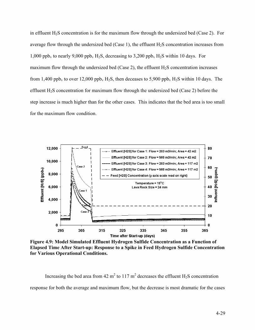
in effluent H2S concentration is for the maximum flow through the undersized bed (Case 2). For

average flow through the undersized bed (Case 1), the effluent H2S concentration increases from

1,000 ppbv to nearly 9,000 ppbv H2S, decreasing to 3,200 ppbv H2S within 10 days. For

maximum flow through the undersized bed (Case 2), the effluent H2S concentration increases

from 1,400 ppbv to over 12,000 ppbv H2S, then deceases to 5,900 ppbv H2S within 10 days. The

effluent H2S concentration for maximum flow through the undersized bed (Case 2) before the

step increase is much higher than for the other cases. This indicates that the bed area is too small

for the maximum flow condition.

Figure 4.9: Model Simulated Effluent Hydrogen Sulfide Concentration as a Function of Elapsed Time After Start-up: Response to a Spike in Feed Hydrogen Sulfide Concentration for Various Operational Conditions.

Increasing the bed area from 42 m2 to 117 m2 decreases the effluent H2S concentration

response for both the average and maximum flow, but the decrease is most dramatic for the cases

4-29

of maximum flow (Case 2 and Case 4). For the maximum flow through a properly sized bed

(Case 4), the effluent H2S concentration increases from 900 to 8,100 ppbv H2S, then decreases to

2,800 ppbv H2S within 10 days. This shows how a sharp influent concentration increase will

pass through the biofilter as an effluent spike and the effluent spike will be higher for an

undersized bed.

Also, Figure 4.8 shows that the effluent H2S concentration will return to a low value

immediately after the influent spike passes through the biofilter. In fact, the effluent

concentration is lower immediately after the completion of the step increase than before it. This

is due to the increase in active biomass concentration in the biofilm after the step increase (data

not shown). The higher substrate concentration during the step increase allows for greater

biomass growth.

4.3.9 Biofilter Construction and Operation. Typically, biofilters have a rectangular or

cylindrical shape although non-rectangular shapes can also be used when there is a space

constraint. An existing tank (such as a clarifier) may also be used. The biofilter may be

enclosed or have an open outlet with the bed directly exposed to the atmosphere. It is crucial to

use construction material that is resistant to corrosion by H2S and sulfuric acid or to use a

durable protective coating. The absence of corners in a cylindrical biofilter will provide better

air distribution, but may be more difficult to fit a liner to; alternatively, a spray-on coating may

be used to line the tank. An air distribution system should collect the contaminated air from the

source and distribute it evenly through the biofilter.

Air conveyance may be by forced draft (with the blower at the influent) or induced draft

(with the blower at the effluent), although induced draft can only be used with a closed biofilter.

The contaminated air is typically top-loaded (down-flow of the contaminated air through the

4-30

biofilter) or bottom-loaded (up-flow), although horizontal flow has been used and step feed and

forward feed may be feasible (Lee et al., 2001). An open outlet biofilter cannot be used for

horizontal flow or down-flow. In an up-flow lava rock biofilter used for H2S removal, the pH

will be lowest at the bottom of the biofilter bed because the biomass concentration is highest

where the H2S concentration is highest (at the influent). Unlike organic bed media, lava rock

requires nutrient addition for microbial growth. This is typically done by irrigating the bed with

water containing the required nutrients; the water also provides essential moisture. Cedar Rapids

WPCF uses spray nozzles to deliver clarified carbonaceous activated sludge effluent providing

nutrients and moisture as well as removing the sulfuric acid from the bed (Martin et al., 2002).

Devinney et al. (pp. 149-174) provide a more detailed description for full-scale biofilter design.

Figure 4.6 and Figure 4.8 show that temperature has a significant influence on biofilter

performance. Hence, it is important to maintain a temperature in the biofilter as close to the

design temperature as possible. The biofilter cover, air feed ducts, and rinse water feed pipes

should all be well insulated, especially in cooler climates. Also, the bed portion of the biofilter

can be located below ground or insulated by adding an earth embankment. Increasing the bed

temperature may be achieved either by heating the feed air or heating the rinse water feed.

However, heating the feed air will decrease the relative humidity of the air, potentially drying out

the biofilter bed.

Model simulations show that as the biofilter temperature increases, the biofilter reaches

the optimum removal efficiency more rapidly, indicating that a summer start-up of a biofilter

would proceed more rapidly (data not shown). This is due to more rapid biofilm development

resulting from faster growth of the microorganisms at higher temperatures. Also, inoculating a

biofilter (e.g. with raw sewage, activated sludge, consortia from food processing industry, or lab

4-31

cultivated microorganisms) may result in a faster start-up but generally does not effect the long-

term performance of the biofilter (Devinney et al., 1999, pp. 83-84, 187). Since the exact origin

of the microorganisms in a lava rock biofilter is unknown (e.g. sewage, lava rock, or elsewhere)

and inoculation does not ensure that the inoculum will adhere to the lava rock, inoculation may

not be so simple and straightforward. Sewage is one possible source of inoculum but pathogens

may be a concern and solids, oil, and grease should be removed to prevent biofilter bed fouling

and clogging. Another source of inoculum is the rinse water from an existing lava rock biofilter.

Since the concentration of microorganisms in the rinse water may be very dilute it may be

beneficial to concentrate them (e.g. using a centrifuge).

4.3.10 Biofilter Configuration. Although the capital cost may be less for a single

biofilter, using two smaller biofilters allows for greater operational flexibility. Using two

biofilters in parallel allows for the isolation of an individual bed for maintenance or during shut

down without interrupting the flow through the other bed. For example, the model predicts that

for average design conditions (20 ppmv feed H2S concentration, 283 m3/min air flow, 17oC

temperature) shown in Case A of Figure 4.8, the effluent H2S concentration will be 800 ppbv for

two 21-m2 biofilters (42 m2 total area) in parallel. If, during maintenance, the feed is switched

from both of the 21 m2 biofilters to a single 21 m2 biofilter, the estimated effluent H2S

concentration will only increase from 800 ppbv to 1,100 ppbv. However, if maximum feed and

low temperature (80 ppmv feed H2S concentration, 566 m3/min air flow, 15oC temperature) is

anticipated, the biofilter area may be sized at 140 m2 for the “worst-case” scenario (Case C in

Figure 4.8). Sizing two biofilters in parallel at 70 m2 each (140 m2 total area) will provide

treatment to 1,400 ppbv in a single bed compared to 1,000 ppbv using both beds for maximum

feed and minimum temperature design conditions.

4-32

Another advantage to using two smaller biofilters is the flexibility to use the two

biofilters in series if necessary in future operation. A biofilter configuration with beds operated

in series allows each individual bed to treat different contaminants. This type of biofilter has

been used successfully to remove both H2S and VOCs combined in a single air stream

(Chitwood et al., 1999; Ruokojarvi et al., 2001; and Li et al., 2003). Removal of both H2S and

VOCs is difficult in a single-bed biofilter because the oxidation of H2S generates sulfuric acid

and the declining pH inhibits the organisms that degrade compounds other than H2S; after H2S is

removed in the first biofilter, a second biofilter can be used to remove other reduced sulfur

compounds and VOCs at neutral pH (Li et al., 2003). Chitwood et al. (1999) used a two-stage

biofilter, the first stage containing lava rock and operating at a low pH and the second stage

containing wood chips operating at neutral pH, to treat a mixed air stream of H2S and VOCs.

Another possible biofilter configuration, is cycled switching of two beds in series. This

involves feeding odorous air to bed 1 with the treated effluent from bed 1 being fed to bed 2. At

the end of the cycle, the feed is switched and odorous air is first fed to bed 2 and the treated

effluent from bed 2 is fed to bed 1. This may allow for higher biomass concentration throughout

the entire bed depth in both biofilters. The higher biomass concentration may also provide for

better treatment of shock loads. A more detailed model simulation could be used to estimate the

switching frequency although pilot testing would be required to verify this. Directional

switching in a single bed has been examined for the control of moisture and biomass growth

(Kinney et al., 1996 and Sabo et al. 1996, p. 63).

Although two beds in parallel or series or with cycled switching may provide more

flexibility and possibly improved treatment, they will have a higher capital cost, will be more

complex to operate, and will have larger head losses. The final choice of bed configuration must

4-33

be based on a detailed cost analysis, which includes evaluating the benefit and likelihood of

potential change in conditions.

4.4 CONCLUSIONS

1. For the design and performance evaluation of biofilters used for removing odorous

compounds, it may be more useful to express the performance in terms of effluent concentration

rather than removal efficiency or elimination capacity. Bed volume (or area for a constant bed

depth) may be more convenient than residence time for sizing the biofilter if the airflow is

constant.

2. A conventional biofilter will be limited to a minimum effluent concentration. Increasing

residence time, increasing bed area or volume, or decreasing loading or flow will not reduce the

effluent concentration below that minimum effluent concentration. However, the minimum

effluent concentration is a function of temperature and will decrease with increasing temperature

(up to the optimum temperature). For the model calibration values outlined in this study, the

minimum effluent concentration decreased from 1,100 ppbv H2S to 800 ppbv H2S when the

temperature was increased from 15oC to 17oC.

3. The effluent concentration from a biofilter may approach the minimum effluent concentration

by increasing the residence time. At sufficiently long residence times, further reduction in the

residence time will only result in a slight reduction in the effluent H2S concentration. For the

average feed conditions in this study, the effluent H2S concentration decreases by 140 ppbv when

4-34

the residence time is increased from 3.7 to 4.5 seconds; when residence time is increased from

5.5 seconds to 9.5 seconds, the effluent H2S concentration decreases by only 100 ppbv.

4. Reducing the packing material size may improve performance for a biofilter that has

insufficient residence time. Replacing 48 mm size lava rock with 12 mm size lava rock for a

biofilter with a 2.9 second residence time at the average feed conditions in this study reduces the

effluent H2S concentration from 4,100 ppbv to 800 ppbv.

5. Shock loading can significantly increase the final effluent H2S concentration above that

predicted by steady-state model simulations. Large influent concentration increases will pass

through the biofilter as an effluent spike and this spike will be higher for an undersized bed. To

consistently meet treatment objectives, dynamic feed conditions should be considered as well as

the combination of low temperature and high flow and feed concentration.

6. Biofilter™ can serve as a valuable tool in the design and performance optimization of

biofilters.

4.5 REFERENCES

BiofilterTM: Biofilter Model Software, Design Option Tool, Version 1.1 (April, 2002) Authors:

Crittenden, J.C.; Mihelcic, J.R.; Li, H.; Oman, E.; and Hautakangas, H. Michigan Technological

University, National Center for Clean Industrial and Treatment Technologies Environmental

Technologies.

Chitwood, D.E.; Devinny, J.S.; and Reynolds, E.F. (1999) Evaluation of a Two-Stage Biofilter

for Treatment of POTW Waste Air. Env. Prog., 18, 212-221.

4-35

Chitwood, D.E., and Devinny, J.S. (2001) Treatment of a Mixed Hydrogen Sulfide and Organic

Vapors in a Rock Medium Biofilter. Water Env. Res., 73(4), 426-435.

Cox, H.H.J., and Deshusses, M.A. (1999) Biomass Control in Waste Air Biotrickling Filters by

Protozoan Predation. Biotechnol. Bioengrg., 62, 216-224.

Crites, R., and Tchobanoglous, G. (1998) Small and DeCentralized Wastewater Management

Systems, WCB McGraw-Hill, Boston.

Dechant, D; Ball, P.; and Hatch C. (1999) Full Scale Validation of Emerging Bioscrubber

Technology for Odor Control. Proc. Water Environ. Fed. 72nd Annu. Conf. Exposition [CD-

ROM], New Orleans, La.

Deshusses, M.A.; Hamer, G.; and Dunn, I.J. (1995) Behavior of Biofilters for Waste Air

Biotreatment. 1. Dynamic Model Development. Environ. Sci. Technol., 29, 1048-1058.

Devinny, J.S.; Deshusses, M.A.; and Webster, T.S. (1999) Biofiltration for Air Pollution

Control. Lewis Publishers, Boca Raton, FL.

De Zwart, J.M.M., and Kuenen, J.G. (1992) C1-cycle of Sulfur Compounds. Biodegradation 3,

37-59.

Fortin, N.Y., and Deshusses, M.A. (1999a) Treatment of Methyl tert-Butyl Ether Vapors in

Biotrickling Filters. 1. Reactor Startup, Steady-State Performance, and Culture Characteristics.

Environ. Sci. Technol., 33(17), 2980-2986.

Fortin, N.Y., and Deshusses, M.A. (1999b) Treatment of Methyl tert-Butyl Ether Vapors in

Biotrickling Filters. 2. Analysis of the Rate-Limiting Step and Behavior under Transient

Conditions. Environ. Sci. Technol., 33(17), 2987-2991.

4-36

Hautakangas, H; Mihelcic, J.R.; Crittenden, J.C.; and Oman, E.J. (1999) Optimization and

Modeling of Biofiltration for Odor Control. Proc. Water Environ. Fed. 72nd Annu. Conf.

Exposition [CD-ROM], New Orleans, La.

Kinney, K.A.; Chang, D.P.Y.; Schroeder, E.D.; and Scow, K.M. (1996) Performance of a

Directionally-switching Biofilter Treating Toluene Contaminated Air” Proc. Air Waste Mgmnt.

Assn. 89th Annu. Meeting Exhibition, Pittsburgh, PA.

Lee, D.H.; Lau, A.K.; and Pinder, K.L. (2001) Development and Performance of an Alternative

Biofilter System. J. Air Waste Mgmnt. Assn., 51, 78-85.

Li, H. (2002) Modeling and Optimization of Biofiltration for Odor Control, PhD dissertation,

Michigan Technological University, Houghton, MI.

Li, H.; Crittenden, J.C.; Mihelcic, J.R.; and Hautakangas, H. (2002) Optimization of Biofiltration

for Odor Control: Model Development and Parameter Sensitivity, Water Environ. Res., 72(1), 5-

16.

Li, H.; Mihelcic, J.R.; Crittenden, J.C.; and Anderson, K.A. (2003) Field Measurements and

Modeling of a Two-Stage Biofilter that Treats Odorous Sulfur Emissions. J. Environ. Eng., in

press.

Martin, R.W.; Li., H.; Mihelcic, J.R.; Crittenden, J.C.; Lueking, D.R.; Hatch, C.R.; and Ball, P.

(2002) Optimization of Biofiltration for Odor Control: Model Verification and Applications.

Water Environ. Res., 72(1), 17-27.

Morton, R., and Caballero, R. (1996) The Biotrickling Story. Water Environ. Technol., 8, 39-45.

Rittman, B.E., and McCarty, P.L. (2001) Environmental Technology: Principles and

Applications. McGraw-Hill, Boston, Ma.

4-37

Ruokojarvi, A.; Ruuskanen, J.; Martikaninen, P.J.; and Olkkonen, M. (2001) Oxidation of Gas

Mixtures Containing Dimethyl Sulfide, Hydrogen Sulfide, and Methanethiol Using a Two-stage

Biotrickling Filter. J. Air Waste Mgmnt. Assn., 51, 11-16.

Sabo, F.; Schneider, T.; and Motz, U. (1996) Latest Developments and Industrial Applications of

Biofiltration. Proc. 1996 Conference on Biofiltration (an Air Pollution Control Technology),

Reynolds, F.E., editor, Reynolds Group, Tustin, CA.

Schowengerdt, R.W.; Hunter, B.; and Hanson, R.E. (1999) Incremental Hydrogen Sulfide Loading

and Diurnal Fluctuation of Three Operating Biofilters. Proc. Water Environ. Fed. 72nd Annu. Conf.

Exposition [CD-ROM], New Orleans, La.

Shareefdeen, Z.; Baltzis, B.C.; Oh, Y.S.; and Bartha, R. (1993) Biofiltration of Methanol Vapor.

Biotechnol. Bioengrg. 41,512-524.

Sorensen, H.W.; Bruciak, J.; Gomez, G.G.; and Ocanas, R. (2000) Engineer-Operator Team

Develops a Cost-Effective System Wide Odor Control Program for the Extremely High Sulfide

Concentrations in the City of Brownsville, Texas. Proc. Water Environ. Fed. 73rd Annu. Conf.

Exposition [CD-ROM], Anaheim, Ca.

Swanson, W.J., and Loehr, R.C. (1997) Biofiltration: Fundamentals, Design, and Operations

Principles, and Applications. J. Env Engrg., 123(6):538-546.

Torres, E.M.; Devinny, J.; Basrai, S.S.; Carson, L.J.; Gossett, R.; Kogan, V.; Ahn, T.; Kardos,

D.; Webster, T.; and Stolin, B. (1979) Biofiltration: Controlling Air Emissions Through

Innovative Technology. Water Environment Research Foundation, Project 92-VOC-1.

Vaith, K.; Cannon, M.; Milligan, D.; and Heydown, J. (1996) Comparing Scrubbing

Technologies. Water Environ. Technol., June, 35-38.

4-38

4-39

Vic, T.E. (2001) Wastewater Treatment Plant Odor Control Using a Lava Rock Based Biofilter.

74th Annu. Central States Water Environ. Assoc. Conf., La Crosse, Wi.

Wallis, M.; Witherspoon, J.; Suzuki, S.; Card, T.R.; Mayer, G.; and Chang, D.P.Y. (1996) A

Critical Review of Odor Control Equipment for Toxic Air Emissions Reduction, Project 91-

VOC-2, Water Environment Research Foundation, Alexandria, Va.

Wani, A.H.; Branion, R.M.R.; and Lau, A.K. (1998) Effects of Periods of Starvation and

Fluctuating of Hydrogen Sulfide Concentration on Biofilter Dynamics and Performance. J.

Hazardous Materials, 60, 287-303.

Wong, E.; Velez, S.I.; and Greer, G. (1999) Effective Odor Control Techniques in Lee County

Sewer Systems. Proc. Water Environ. Fed. 72nd Annu. Conf. Exposition [CD-ROM], New

Orleans, La.

Yang, Y., and Allen, E.R. (1994) Biofiltration Control of Hydrogen Sulfide. 1. Design and

Operational Parameters. J. Air Waste Mgmt. Assn., 44, 863-868.

CHAPTER 5 CONCLUSIONS AND RECCOMENDATIONS 5.1 CONCLUSIONS: Chapter 1, Conclusion 1: Chemoautotrophic bacteria play an important role in wastewater

treatment processes. Nitrifying bacteria are responsible for the removal of ammonia and

nitrogen from wastewater and various Acidithiobacillus sp. have been shown to remove

hydrogen sulfide from odorous air.

2.1 Dye-bearing wastewater containing the azo dye acid black 1 (AB1) inhibited nitrification at

concentrations as low 24 mg AB1/L. The combined effect of low temperature and dye-bearing

wastewater caused complete nitrification failure at 7oC while nitrification inhibition at 22oC was

less, but still significant: 97.0% NH3 removal for 73 mg AB1/L compared to 99.9% for the 22oC

control.

2.2 Ammonia (NH3) and chemical oxygen demand (COD) removal declined in all reactors fed

AB1 with the performance decline occurring sooner as the concentration of AB1 increased. For

24 mg AB1/L, 49 mg AB1/L, and 73 mg AB1/L, the nitrification failure occurred in 52 days, 45

days, and 38 days after start-up, respectively.

2.3 Decreasing AB1 loading at 7oC led to partial nitrification recovery within one week as

indicated by significant nitrate production and a slight improvement in COD removal. There

was no corresponding increase in NH3 removal, however.

5-1

2.4 The presence of AB1-bearing wastewater led to additional deterioration. COD removal

decreased at 7oC and 22oC; effluent TSS increased at 7oC; endogenous and exogenous oxygen

uptake decreased and foaming increased at 7oC.

2.5 The combination of AB1 and low temperature caused poor effluent quality at 7oC,

emphasizing that potential inhibitors must be investigated at the lowest WWTP operating

temperature.

3.1 A dynamic biofilter model predicting the removal of hydrogen sulfide (H2S) in biofilters was

calibrated and validated using pilot-scale and full-scale data. The model calibration simulation

agreed well with the actual pilot-scale data. The model validation simulations of the pilot- and

full-scale biofilter also agreed well with actual data. The model used in this study has been

incorporated into a user-friendly software package (BiofilterTM).

3.2 Model simulations of the full-scale biofilter using the parameters determined from the model

calibration illustrate the influence of gas residence time, influent concentration, temperature, and

changes in influent concentration on biofilter performance and design.

3.3 Model simulations showed that the lava rock biofilter should provide at least 5 seconds of

residence time to achieve a treatment objective of 0.5 ppmv; the time the biofilter takes to

achieve the steady-state treatment objective of 0.5 ppmv increases from less than 1 day to 2 to 3

days as the temperature is decreased from 25 to 15oC.

3.4 Model simulations indicated that it is useful to consider the influent concentration in biofilter

design.

5-2

3.5 Model simulations also showed the need to consider the maximum influent concentration

instead of the average influent concentration when sizing a biofilter.

4.1 Biofilter™ is a valuable tool for the design and performance evaluation of biofilters.

4.2 Expressing performance in terms of effluent concentration rather than removal efficiency or

elimination capacity may be more useful in the design and performance evaluation of biofilters.

Bed volume may be more convenient than residence time for sizing the biofilter receiving

constant airflow.

4.3 Increasing residence time, bed area, or volume, or decreasing loading or flow will not reduce

the effluent concentration below the minimum effluent concentration. However, the minimum

effluent concentration decreases with increasing temperature (up to the optimum temperature).

4.4 Increasing the biofilter residence time may result in the effluent concentration approaching

the minimum effluent concentration. A further reduction in the residence time will only result in

a slight reduction in the effluent H2S concentration at higher residence times. For the average

feed conditions in this study, the effluent H2S concentration decreases by 140 ppbv when the

residence time is increased from 3.7 to 4.5 seconds; when residence time is increased from 5.5

seconds to 9.5 seconds, the effluent H2S concentration decreases by only 100 ppbv.

4.5 For a biofilter that has insufficient residence time, reducing packing material size may

improve performance. For a biofilter with a 2.9 second residence time at the average feed

conditions in this study, effluent H2S concentration was reduced the from 4,100 ppbv to 800 ppbv

by replacing 48 mm size lava rock with 12 mm size lava rock.

5-3

5-4

4.6 Shock loading significantly increased the final effluent H2S concentration above that

predicted by steady-state model simulations. Large influent concentration increases will pass

through the biofilter as an effluent spike and this spike will be higher for an undersized bed. To

consistently meet treatment objectives, dynamic feed conditions should be considered as well as

the combination of low temperature and high flow and feed concentration.

5.2 RECOMMENDATIONS:

1. Performing additional nitrification inhibition studies using AB1 (instead of industrial dyeing

discharge) and run at varying substrate (NH3) concentrations can be used to determine the type

of inhibition, whether it is reversible, and values of the inhibition coefficient. Model simulations

could be used to evaluate potential alternate treatment methods. Measuring the concentration of

AB1 at the inlet and outlet would provide useful information on dye removal.

2. Additional full-scale data using continuous data acquisition would provide a better basis for a

full-scale model validation.

3. A detailed study of the biochemical processes occurring in a red lava rock biofilter used for

H2S removal would provide information useful for determining the BiofilterTM model input

parameters. To determine if any abiotic reactions occur, H2S removal using a column of

sterilized lava rock (e.g. autoclaved) at low pH could be ascertained.

4. BiofilterTM could be upgraded to allow for variable temperature input by subroutines that

calculate the temperature-dependant variables (e.g. µmax, Db, and H) as a function of temperature.

APPENDIX A BIOFILTERTM CALIBRATION AND VALIDATION ACCOUNTING FOR VARIABLE FLOW AND DEPTH PROFILE OF HYDROGEN SULFIDE CONCENTRATION A.1 INTRODUCTION

Data from the Cedar Rapids Water Pollution Control Facility pilot-scale and full-scale

biofilters was used to calibrate and validate the model presented by Li et al. (2002). The user-

friendly software BiofilterTM (Crittenden et al., 2002) was used to obtain model parameter

values. The original solution resulting in the model parameters used in the original calibration

and validation presented in Chapter 3 may be only one of several possible solutions. This

solution was obtained from initial estimates of the parameters based on literature citations and

engineering judgment. However, limiting a solution to these rules may preclude other potential

solutions that may provide insight into unexpected chemical-physical processes. Furthermore,

the solution obtained in Chapter 3 was based on several simplified assumptions (discussed

below). Additional data and information on actual process conditions allows for more

representative calibration and validation solutions. Finally, the existence of multiple solutions

forces the user to consider the conceptual model rather than simply using the software to crank

out numbers without considering the meaning behind those numbers and the limitations to the

model. When faced with multiple solutions, engineers must use their knowledge and judgment

to decide which solution is best for the given circumstances.

A-1

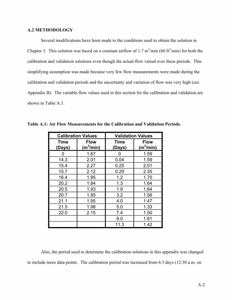
A.2 METHODOLOGY

Several modifications have been made to the conditions used to obtain the solution in

Chapter 3. This solution was based on a constant airflow of 1.7 m3/min (60 ft3/min) for both the

calibration and validation solutions even though the actual flow varied over these periods. This

simplifying assumption was made because very few flow measurements were made during the

calibration and validation periods and the uncertainty and variation of flow was very high (see

Appendix B). The variable flow values used in this section for the calibration and validation are

shown in Table A.1.

Table A.1: Air Flow Measurements for the Calibration and Validation Periods.

Calibration Values Validation Values Time Flow Time Flow

(Days) (m3/min) (Days) (m3/min) 0 1.67 0 1.59

14.3 2.01 0.04 1.59 15.4 2.27 0.25 2.01 15.7 2.12 0.29 2.35 16.4 1.95 1.2 1.70 20.2 1.84 1.3 1.64 20.5 1.93 1.9 1.64 20.7 1.95 3.2 1.56 21.1 1.95 4.0 1.47 21.5 1.98 5.0 1.33 22.0 2.15 7.4 1.50

9.0 1.81 11.3 1.42

Also, the period used to determine the calibration solutions in this appendix was changed

to include more data points. The calibration period was increased from 6.3 days (12:30 a.m. on

A-2

March 8, 2000 and ending at 7:30 a.m. on March 14, 2000) in the Chapter 3 solution to 6.7 days

(11:30 p.m. on March 7, 2000 and ending at 6:30 p.m. on March 14, 2000) for the solutions

determined in this section. While the calibration period only lasted for between 6.3 days and 6.7

days, the actual model simulation covered several weeks of operation because the actual pilot-

scale biofilter was in operation before the data was collected for the calibration and validation

periods. Li (2002, pp. 244-258) provides the actual data used for the model input of the influent

H2S concentrations and the measured effluent H2S concentrations.

In addition to the calibration period, the density of the lava rock used in the biofilter was

corrected from 4.0 g/cm3 to 1.13 g/cm3. This density and the bed porosity (ε) of 0.40 were used

to recalculate the mass of the lava rock (Li, 2002, p. 209). Using the bed diameter of 0.61 m and

the bed depth of 1.83 m, the bed volume in the pilot scale biofilter was determined to be 0.53 m3.

Although mass (M) is generally equal to volume (V) multiplied by density (ρ), the empty space

between the packing material must be accounted for in a biofilter bed. This is corrected using ε,

defined as the ratio of void volume to total volume. Hence, the mass of the lava rock packing

material in the pilot-scale biofilter is determined as follows:

M = ρV(1-ε) = 1,130 kg/m3 (0.53 m3)(1-0.4) = 362 kg (A.1)

Finally, the time average influent H2S concentration was recalculated to include the total run

time input into the model. Although this input parameter had only a negligible effect on the

model output for the calibration and validation in this section, it had a small, but noticeable effect

on the model simulations run to steady state in Chapter 4. The original values used in Chapter 3

and the corrected values used in this section are listed in Table A.2.

After the parameters in Table A.2 were corrected, additional parameters were adjusted to

obtain new calibration and validation solutions. The adjusted parameters are: biofilm diffusivity

A-3

(Db), sphericity (φ), yield coefficient (Y), half saturation constant (Ks), maximum specific growth

rate (µmax), minimum biofilm concentration (Cxmin), maximum biofilm concentration (Cxmax), and

initial biofilm concentration (Cxo). These parameters were examined outside of the range

specified in Martin et al. (2002) so as not to preclude any potential solutions not considered in

the original solution. As in Chapter 3, the calibration and validation solutions were determined

by minimizing the objective function (OF) defined in Equation 3.1. However, the sum of the

residuals (Equation 3.2) was not included as a criterion because it can be misleading: a

comparable number of large negative and positive residuals can cancel each other out. This can

be overcome by using the sum of the absolute value of the residuals as follows:

n

Σ |(Cdata,i – Cmodel,i)/Cmodel,i | (A.2) i=1

Where

n = the number of data points,

Cdata,i = measured effluent concentration, and

Cmodel,i = effluent concentration predicted by the model.

In addition to the sum of the absolute value of the residuals and the OF, the H2S

concentration profile throughout the depth of the biofilter between the influent and effluent was

used to evaluate the accuracy of the model solution. The H2S concentration was manually

measured from the digital readout of a Conspec meter at various biofilter bed depth locations

between the influent and effluent made at several different times during the calibration period.

The samples were drawn from 9 mm (3/8 inch) ID stainless steel sampling tubes inserted

approximately 25 cm (10 inches), radially toward the column center, at several bed depth

locations between the influent and effluent. The wall of these sampling tubes had 3 mm (1/8

A-4

inch) holes drilled along their length with the holes aligned upward, allowing samples to be

drawn from throughout the radial length of the bed. Model simulated values of the H2S

concentration were determined throughout the depth of the biofilter between the influent and

effluent by using an input of 12 axial elements (the bed depth was divided into 12 elements of

equal length). The model simulated values were compared to the manual H2S concentrations

measured at the various biofilter depths.

Table A.2: Comparison of Original and Corrected Model Input Values.

Calibration Values Validation Values Original New Original New Parameter

(Chapter 3) (Appendix A) (Chapter 3) (Appendix A)Time Period (days) 6.3 6.7 10 10

Influent Flow (m3/min)

1.7 (average)

Variable (see Table A.1)

1.7 (average)

Variable (see Table A.1)

Average Influent H2S Concentration (mg/L) 0.139 0.216 0.139 0.216

Density of Lava Rock (g/cm3) 4.00 1.13 4.00 1.13

Mass of Lava Rock (kg) 1,280 362 1,280 362

All of the model simulations were run individually and the resulting model simulated H2S

concentrations were manually cut and pasted into a MicrosoftTM Excel Spreadsheet to determine

the OF and sum of the absolute value of the residuals for each simulation. Model simulations

were run for both the calibration and validation. Also, the effluent H2S concentration as a

function of time and the H2S concentration as a function of bed depth were plotted for both the

model simulated values and the measured values to allow for visual comparison.

A-5

A.3 RESULTS AND DISCUSSION

Initially, each model parameter was individually varied to obtain the minimum OF. To

obtain further solutions, combinations of φ, Y, Ks, and µmax were varied; then, Cxmin, Cxmax, and

Cxo were varied to fine-tune the solution. The value for Db obtained in the first re-calibration

solution was retained for future simulations. Several hundred model simulations were run

spanning a large range of values of the model parameters (see Table A.3). These model

simulations resulted in four potential solutions. In future studies, a genetic algorithm may

eliminate the tedious manual trial-and-error method required in this study.

Table A.3: Range of Model Parameters Used in Determining the Re-Calibration and Re-Validation Solutions and Original Parameter Values used by Martin et al. (2002).

Original Values (1) Parameter (units) Range in this study Calibration Validation

φ (unitless) 0.1 to 0.7 0.5 0.5 Y (g cells/g-mole H2S) 0.005 to 25 3.8 3.8

Ks (µmol/L) 0.02 to 133 3.5 3.5 µmax (1/hr) 0.048 to 150 0.275 0.200 Cxo (g/L) 0.05 to 120 10 6

Cxmin (mg/L) 4 to 500 10 10 Cxmax (g/L) 66 to 2,000 100 100 Db (cm2/s) 1.68 to 12 4.65x10(-6) 3.60x10(-6)

(1) from Martin et al. (2002)

Figure A.1 shows the model simulated effluent H2S concentrations as a function of time

for the calibration period; the curves show the original solution (Chapter 3) for constant flow, the

original solution for variable flow, and Solution 1 of the re-calibration. Although the model

output for the original calibration (Chapter 3) agrees well with the measured data for constant

flow, there is a sharp increase in the effluent H2S concentration (from 2.0 to 7.8 ppbv) when

A-6

variable flow is introduced. The effluent H2S concentration is even higher when the corrected

model input values from Table A.2 are included (data not shown). Solution 1 provides a

comparable fit to the original solution, although the effluent H2S concentration is slightly higher

than the original solution during the initial influent spike and slightly lower than the original

solution during the more stable final period.

Figure A.1: Comparison of the Output from Various Model Calibration Conditions to the Measured Data for Pilot Scale Biofilter: Effluent Hydrogen Sulfide Concentration as a Function of Time.

Figure A.2 shows model simulated effluent H2S concentrations as a function of time for

the validation period; the curves show the original solution (Chapter 3) for constant flow, the

original solution for variable flow and corrected values (Table A.2), and Solution 1 of the re-

validation. Solution 1 provides a comparable fit to the original solution, although the effluent

H2S concentration is slightly lower than the original solution during the initial start-up period,

which is shown at the beginning of the plot. Unlike the calibration period, the model output

A-7

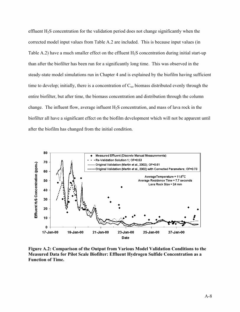
effluent H2S concentration for the validation period does not change significantly when the

corrected model input values from Table A.2 are included. This is because input values (in

Table A.2) have a much smaller effect on the effluent H2S concentration during initial start-up

than after the biofilter has been run for a significantly long time. This was observed in the

steady-state model simulations run in Chapter 4 and is explained by the biofilm having sufficient

time to develop; initially, there is a concentration of Cxo biomass distributed evenly through the

entire biofilter, but after time, the biomass concentration and distribution through the column

change. The influent flow, average influent H2S concentration, and mass of lava rock in the

biofilter all have a significant effect on the biofilm development which will not be apparent until

after the biofilm has changed from the initial condition.

Figure A.2: Comparison of the Output from Various Model Validation Conditions to the Measured Data for Pilot Scale Biofilter: Effluent Hydrogen Sulfide Concentration as a Function of Time.

A-8

Figure A.3 shows the model simulated effluent H2S concentrations for all four re-

calibration solutions. All four solutions are comparable, although the effluent H2S concentration

for Solution 4 is significantly lower than the other three solutions during the more stable final

period. Similarly, Figure A.4 shows the model simulated effluent H2S concentration for all four

re-validation solutions. All four solutions result are comparable, although the effluent H2S

concentration is slightly lower for Solution 3 during the initial start-up period and has slightly

higher peaks for Solution 4 after the initial start-up period.

Figure A.3: Comparison of Re-calibration Solutions: Effluent Hydrogen Sulfide Concentration as a Function of Time.

The OF and sum of the absolute value of the residuals for the re-calibration and re-

validation and the original solutions are listed in Table A.4. This provides a quantitative

evaluation tool to supplement the qualitative evaluations of Figures A.1, A.2, A.3, and A.4. The

values of the OF and sum of the absolute value of the residuals for the solutions determined in

A-9

the re-calibration are comparable to those in the original solution using constant flow and

uncorrected input values. However, when the variable flow and the other corrected input values

(from Table A.2) are used with the original solution, the values of the OF and sum of the

absolute value of the residuals are significantly higher for the original calibration solution. This

indicates that the fit of the corrected original calibration solution to the data is not as good as the

other calibration solutions. The fit of the corrected original validation solution is only slightly

worse than the uncorrected original validation solution.

Figure A.4: Comparison of Re-validation Solutions: Effluent Hydrogen Sulfide Concentration as a Function of Time.

A-10

Table A.4: Comparison of Objective Function and Sum of Absolute Value of Residuals for Re-calibration, Re-validation, and Original Solution.

Calibration Validation

Solution Objective Function

Sum of |Residuals|

Objective Function

Sum of |Residuals|

Solution 1 0.40 0.33 0.53 0.46 Solution 2 0.39 0.32 0.57 0.48 Solution 3 0.42 0.34 0.56 0.49 Solution 4 0.47 0.41 0.62 0.51

Original Solution (1) 0.42 0.35 0.61 0.52 Original Solution

for corrected values (2) 1.31 1.01 0.69 0.57

(1) Original Solution from Martin et al. (2002) for constant flow; OF re-calculated for new period. (2) Original Solution from Martin et al. (2002) for variable flow (all corrected model input values from Table A.2 are used in the validation); OF re-calculated for new period.

Figure A.5 shows the H2S concentration profile through the depth of the biofilter bed

between the influent and effluent for the actual data and for the model simulations for the four

different solutions. The values for the actual data shown in Figure A.5 are averages from seven

manual depth concentration measurements made each day from Mach 12, 2000 through Mach

14, 2000. At high H2S concentrations (near the influent) the error bars represent the 95%

confidence limits; at low H2S concentrations (greater than 40 cm from the influent) the error bars

represent the uncertainty of the Conspec meter (see Appendix B). The values for the model

simulation outputs shown in Figure A.5 are the averages from model simulation outputs

corresponding to the times of the manual depth concentration measurements. Because the

influent H2S concentration changed over time, normalized H2S concentrations (obtained by

dividing by the H2S concentration by the influent H2S concentration) were used. The original

model calibration solution (Chapter 3) predicts a much higher H2S concentration throughout the

bed depth between the influent and effluent than shown by the actual data. Solution 1 and

A-11

Solution 2 provide the best fit to the actual data for the first 40 cm from the influent; Solution 4

provides the best fit to the actual data for the bed depth from 40 cm to 90 cm from the influent.

Although significantly better than the original solution, the depth profile for Solution 3 is higher

than the actual data for the first 100 cm from the influent.

Figure A.5: Comparison of Original and Re-calibration Solutions to Measured Data: for Bed Profile of Hydrogen Sulfide Concentration as a Function of Distance from Influent.

It is important to note that a majority of the H2S is removed in the portion of the biofilter

bed nearest to the influent. The model simulations indicate that the highest concentration of

active biomass is located in the biofilter nearest to the influent. According to the data, 85% H2S

removal occurs within the first 30 cm (12 inches) from the influent and over 97% removal occurs

within the first 46 cm (18 inches) from the influent. The model simulation for Solution 1

predicts that 78% H2S removal occurs within the first 30 cm (12 inches) from the influent and

90% removal occurs within the first 46 cm (18 inches) from the influent.

A-12

Examination of the Monod equation provides insight into the reaction rate at low and

high substrate concentrations. According to the Monod equation, the specific growth rate, µ

(1/time), can be expressed as follows:

µ = µmax [H2S]/(Ks + [H2S]) (A.3)

Where

µmax = maximum specific growth rate (1/time)

Ks = half-saturation constant (moles/volume)

[H2S] = hydrogen sulfide concentration in the biofilm (moles/volume)

At low substrate concentrations, where Ks >> [H2S], the Monod equation reduces to first-order

kinetics:

µ = µmax [H2S]/Ks (A.4)

At high substrate concentrations, where Ks << [H2S], the Monod equation reduces to zero-order

kinetics:

µ = µmax (A.5)

Figure A.5 shows that near the effluent, the H2S concentration is very low. For the

original solution (from Chapter 3), the model simulated depth-average H2S concentration in the

biofilm at the effluent is 0.0017 µmol/L, compared to a Ks of 3.5 µmol/L; for Solution 1, the

model simulated depth-average H2S concentration in the biofilm at the effluent is 0.0009

µmol/L, compared to a Ks of 18 µmol/L. For all solutions (the four re-calibration solutions in

this Appendix and the original solution from Chapter 3), the depth-average H2S concentration in

the biofilm near the effluent is much lower than Ks and the reaction kinetics are first-order

according to Equation A.4. Using the 250-ppmv peak influent H2S concentration in the gas-

phase (from Figure 3.2 in Chapter 3), the maximum H2S concentration in the biofilm at the

A-13

influent is 27 µmol/L, which is the same order of magnitude as Ks for all solutions. Therefore,

throughout the biofilter bed, the reaction rate is always greater than zero order and approaches

first order as the location in the biofilter approaches the effluent.

Table A.5 lists the new values of the model parameters for each solution determined in

the re-calibration. Table A.6 lists the model parameters for each solution determined in the re-

validation (model parameter which were unchanged from the re-calibration to re-validation are

listed in Table A.5).

Table A.5: Model Parameters from Re-calibration Solutions.

Re-calibration Parameter Values Parameter (units) Solution 1 Solution 2 Solution 3 Solution 4

φ (unitless) 0.50 0.25 0.225 0.50 Y (g cells/g-mole H2S) 0.15 0.50 1.00 0.30

Ks (µmol/L) 18.0 18.0 10.0 21.5 µmax (1/hr) 0.30 0.25 0.20 0.25 Cxo (g/L) 10 12 13 10

Cxmin (mg/L) 10 10 10 100 Cxmax (g/L) 100 100 100 1,000 Db (cm2/s) 2.18x10(-6) 2.18x10(-6) 2.18x10(-6) 2.18x10(-6)

Comparison of the model parameters from the original solution (Table A.3) to those for

the re-calibration and re-validation solutions shows that many parameters were changed, some

by an order of magnitude. Some values did not change: φ (for Solution 1 and Solution 4), Cxo

(for Solution 1 and Solution 4, re-calibration), and Cxmax and Cxmin (for Solution 1, Solution 2,

and Solution 3). The values of µmax in the re-calibration and re-validation solutions were only

slightly smaller or larger than the value in the original solution. Also, Db was lower in the re-

calibration and re-validation solutions, possibly due to the uncertainty in the biofilm thickness,

A-14

which was used to estimate Db (Fan et al., 1990). The lower value of Db indicates that the H2S

diffuses through biofilm more slowly.

Table A.6: Model Parameters from Re-validation Solutions.

Re-validation Parameter Values Parameter (units) Solution 1 Solution 2 Solution 3 Solution 4

µmax (1/hr) 0.072 0.060 0.048 0.060 Cxo (g/L) 3.2 4.0 4.2 10

Db (cm2/s) 1.68x10(-6) 1.68x10(-6) 1.68x10(-6) 1.68x10(-6)

The values for φ in Solution 2 and Solution 3 are lower than from the original solution

determined in Chapter 3. The depth concentration profile for the model output better fit the

measured data when φ was decreased. For a non-spherical object, φ is defined as the ratio of the

surface area of an equivalent volume sphere to the actual surface area of the object; φ = 1 for a

spherical object. For the porous lava rock, the surface area of the pores should be considered if

the pores are not filled with water. While Li (2002, pp.203-208) concluded that the pores were

filled with water, this was based on a laboratory analysis that did not consider the larger pores

(>0.6 mm) and a calculation of capillary rise that does not consider the non-homogeneity and

interconnectedness of the pores present in lava rock (Saar, 1998). Thus, if there is biofilm

growth on the surface of the pores, φ will decrease. Also, since φ is used for determining the

specific active biofilm area by BiofilterTM, a heterogeneous biofilm geometry would decrease φ

(if the biofilm were not covered with water). Gjaltema et al. (1994) point out that biofilm non-

homogeneity can increase the surface area of the biofilm available for mass transfer more than an

order of magnitude.

A-15

In Solution 4, Cxmin and Cxmax are ten times higher than from the original solution

determined in Chapter 3. These high concentrations of active biomass in the biofilm seem

unlikely since observations of the lava rock taken from the biofilter showed no visible sign of a

biofilm and microbial analysis indicated a low number of microorganisms (Li, 2002, pp. 214-

230). Also, small changes in Cxo did not significantly change the effluent H2S concentration for

the calibration period; Cxo was varied to fine-tune the validation in order to obtain a lower OF.

The value of Cxo was higher in the calibration than in validation (except for Solution 4, for which

they were equal). This can be explained by a higher concentration of active biomass in the

biofilm at initial start-up during the calibration period than at initial start-up during the

validation. The calibration period came after the validation and the biofilter was shut down in

between; thus, active biomass (at a higher initial active biomass concentration) may have lain

dormant within the biofilter bed between the validation and calibration periods.

The most significant changes in the values for the model parameters were for Y and Ks.

Ks was increased by three to six times and Y was decreased to between 4% and 25% of the

values from the original solution (from Chapter 3). The depth concentration profile for the

model better fit the measured data by simultaneously increasing Ks and decreasing Y. A

decrease in Y represents a decrease in biomass formation per unit of substrate (H2S) consumed.

A higher Ks represents a higher substrate concentration necessary for the specific growth rate to

approach the maximum specific growth rate for that substrate. In wastewater treatment, a higher

Ks represents a less easily biodegradable compound.

One possible explanation for the lower Y and higher Ks is another microorganism in the

biofilter bed. In fact, the original parameter estimation was based on Acidithiobacillus

thiooxidans, not A. ferrooxidans because little information on the biokinetic parameters for A.

A-16

ferrooxidans was available (Martin, et al., 2002). Li (2002, pp. 214-230) suggested that the H2S

might actually be reacting with the iron released from the lava rock at low pH. If some of the

substrate (H2S) is reacting with the iron, it does not directly result in biomass formation, thus

lowering the apparent yield. It would also mean that a higher concentration would be required to

approach the maximum specific growth rate, Ks.

It may even be possible that the model input parameters are different in different parts of

the biofilter. Since the pH and H2S concentration change with the depth of the bed, it is likely

that some of the model parameters will change with pH so it is likely that various model

parameters will also change with the depth of the bed. In fact, completely different microcosms

may exist at the bottom and top of the column. For example, another sulfide-utilizing

microorganism (e.g. A. thiooxidans) may be present at the top of the biofilter bed. The lava rock

sample used in the microbial analysis indicating A. ferrooxidans was taken from the bottom of

the biofilter bed.

Ultimately, one solution must be chosen when using BiofilterTM in a design and

optimization application. Although the range of solutions can be used to illustrate the range of

uncertainty in the model simulated output (see Appendix B), the engineer must choose the best

solution. Solution 1 was chosen as the best solution for the model parameter input values used in

Chapter 4. Solution 1 had the lowest total sum of the OF and sum of absolute value of residuals,

although Solution 2 and Solution 3 had only slightly higher values. Solution 4 was eliminated

because the model simulated output included negative biomass concentrations at the biofilm

surface in the top of biofilter bed for high loading conditions (data not shown). Also, Solution 3

did not fit the depth profile as well as Solution 1 and Solution 2. Finally, although Solution 2

A-17

provided results similar to Solution 1, it was excluded because φ would most likely be closer to

0.50 (Solution 1) than to 0.25 (Solution 2).

A.4 CONCLUSIONS

1. More than one numerical solution to the model may be possible, and examination of these

solutions may provide insight into poorly understood processes.

2. By comparing the model output to the actual data and observations, some solutions may be

eliminated while others may be considered likely.

3. While multiple numerical solutions to the model may be obtained, the best solution must be

chosen for future use of model applications.

4. The parameters in Solution 1 were chosen for the design and optimization applications in

Chapter 4.

A.5 REFERENCES

BiofilterTM: Biofilter Model Software, Authors: J.C. Crittenden, H. Hautakangas, H. Li, J.R.

Mihelcic, E. Oman, Michigan Technological University, National Center for Clean Industrial

and Treatment Technologies Environmental Technologies Design Option Tool, Version 1.1,

released, April, 2002.

Fan, L.-S.; Leyva-Ramos, R.; Wisecarver, K.D.; and Zehner, B.J. (1990) Diffusion of Phenol

Through a Biofilm Grown on Activated Carbon Particles in a Draft-Tube Three-Phase Fluidized-

Bed Bioreactor. Biotechnol. Bioeng., 35, 279.

A-18

A-19

Gjaltema, A., Arts, P.A.M., van Loosdrencht, M.C.M., Kuenen, J.G., and Heijnen, J.J. (1994)

“Heterogeneity of Biofilms in Rotating Annular Reactors: Occurrence, Structure, and

Consequences”, Biotechnol. Bioeng., 44, 194.

Li, H. (2002) Modeling and Optimization of Biofiltration for Odor Control, PhD dissertation,

Michigan Technological University, Houghton.

Li, H., J.R. Mihelcic, J.C. Crittenden, K.A. Anderson (2002) Field Measurements and Modeling

of a Two-Stage Biofilter that Treats Odorous Sulfur Emissions. Journal of Environmental

Engineering, in press.

Martin, RW, H Li., JR Mihelcic, JC Crittenden, DR Lueking, CR Hatch, P Ball (2002)

Optimization of biofiltration for odor control: Model Verification and Applications. Water

Environment Research. 72(1): 17-27.

Saar, M.O. (1998) The Relationship Between Permeability, Porosity, and Microstructure in

Vesicular Basal, MS thesis, University of Oregon, Eugene.

APPENDIX B UNCERTAINTY IN MODEL SIMULATED EFFLUENT HYDROGEN SULFIDE CONCENTRATION

Because of the uncertainty in many of the model input parameters, there is a large

uncertainty in the model simulated effluent H2S concentration. It is difficult to quantify this

uncertainty in the model simulated effluent H2S concentration. However, the uncertainty of a

single parameter can be used to approximate the uncertainty in the model simulated effluent H2S

concentration for that specific parameter. The parameter uncertainty can be expressed as the

95% confidence limit (+ 2 standard deviations) and both the high and low limits are separately

plugged into the model producing two separate simulated effluent H2S concentrations which

represent the 95% confidence limit for that parameter. Plots of the effluent H2S concentration as

a function of time showing both the high and low 95% confidence limits for a specific model

input parameter provides a more easily understood visual representation of the uncertainty in the

model simulated effluent H2S concentration.

For the calibration and validation in Chapter 4 and Appendix A, the greatest uncertainty

of the measured values is for the temperature and flow measurements. The biofilter temperatures

measured at various bed locations and for the feed air varied from 16oC to 27oC (61oF to 81oF)

over the course of the calibration period and from 3oC to 18oC (37oF to 65oF) over the course of

the validation period of the pilot-scale biofilter. At any time, the bed temperature varied

throughout the bed depths and in the radial direction from the center. During very cold periods,

the edges of the pilot biofilter bed were significantly colder than the bed center. Figure B.1

shows a plot of several temperature measurements at various biofilter locations made during the

B-1

calibration period. Although the bed temperature varied widely, an average bed temperature of

20.2oC (68.4oF) was used for the entire calibration period because the model software currently

only allows for a single constant input of temperature-dependent variables. The temperature

varied even more during the validation period and even fewer temperature measurements were

made. An average bed temperature of 11.5oC (52.7oF) was used for the validation period.

Figure B.1 Biofilter Temperature as a Function of Time at Various Biofilter Bed Locations During Calibration Period.

Figure B.2 shows the model simulated effluent H2S concentration for the Solution 1 re-

calibration bounded by the uncertainty estimate due to temperature. The upper 95% confidence

limit of temperature was 24.0oC (75.2oF) and the lower limit was 16.4oC (61.5oF). Compared to

Solution 1, the model-simulated effluent H2S concentration is much lower using the upper 95%

confidence limit of temperature and much higher using the lower 95% confidence limit of

temperature. During the influent H2S concentration spike at the beginning of the calibration

period, the maximum effluent H2S concentration is 2.6 ppmv at 20.2oC compared to 0.8 ppmv

B-2

and 7.3 ppmv using the upper (24.0oC) and lower (16.4oC) 95% confidence limits of temperature,

respectively.

Figure B.2 Model Simulated Effluent H2S Concentration for Solution 1 Re-calibration Showing Temperature Uncertainty Approximation.

During the more stable influent H2S concentration at the end of the calibration period, the

minimum effluent H2S concentration is 0.2 ppmv at 20.2oC compared to 0.05 ppmv and 0.7 ppmv

using the upper (24.0oC) and lower (16.4oC) 95% confidence limits of temperature, respectively.

Plots of the Solution 2, Solution 3, and Solution 4 (determined in Appendix A) re-calibration

temperature uncertainties are similar those in Figure B.2 although the maximum effluent H2S

concentration spike at the beginning of the calibration period is only 5.4 ppmv at the lower

(16.4oC) 95% confidence limit of temperature (data not shown). It must be pointed out that these

are only estimates; it is not strictly accurate to use only a single temperature input if the

temperature actually varies with time and location as is the case shown in Figure B.1.

B-3

Figure B.3 shows the model simulated effluent H2S concentration for the Solution 1 re-

validation with the approximated uncertainty due to temperature. The upper 95% confidence

limit of temperature was 18.2oC (64.8oF) and the lower limit was 4.8oC (40.6oF). Compared to

Solution 1, the model-simulated effluent H2S concentration is much lower using the upper 95%

confidence limit of temperature and much higher using the lower 95% confidence limit of

temperature. During the initial start-up period, the maximum effluent H2S concentration is 49

ppmv at 11.5oC compared to 22 ppmv and 95 ppmv using the upper (18.2oC) and lower (4.8oC)

95% confidence limits of temperature, respectively. Figure B.3 also shows that at higher

temperatures, the effluent H2S concentration peak is more effectively suppressed. The maximum

effluent H2S concentration peak occurs on January 17, 2000 using 18.2oC compared to January

19, 2000 using 4.8oC. At the end of the validation period (approximately a week after start-up),

the minimum effluent H2S concentration is 2 ppmv at 11.5oC compared to 0.1 ppmv and 13 ppmv

using the upper (18.2oC) and lower (4.8oC) 95% confidence limits of temperature, respectively.

Plots of Solution 2, Solution 3, and Solution 4 (determined in Appendix A) re-validation using

the temperature uncertainty are similar to Figure B.2; however, the maximum effluent H2S

concentration peak at the beginning of the validation period ranges from 92 ppmv to 120 ppmv

using the lower (4.8oC) 95% confidence limit of temperature for Solution 3 and Solution 4,

respectively (data not shown).

There is also uncertainty in the airflow, which was determined from the feed air velocity

measured with three different hand-held digital anemometers. Two were hot wire anemometers

(Dwyer Series 471 and Extech) and one was a mechanical vane type anemometers (Pacer

DA40V). The measurement was made at the center of the feed pipe over the course of the

calibration and validation periods. The velocity measurement varied significantly with time,

B-4

even over a one-minute time period; at any time, the velocity measurement varied with location

in the cross-section of the feed pipe. Figure B.4 shows a plot of several minimum and maximum

feed velocity measurements made during the calibration period. Although the velocity varied

widely during a short time-period, average velocities (averaged over a 0.5-hour to 4-hour time

period) were used as input for the model re-calibration simulations. Also no velocity

measurements were made from 11 a.m. on March 9, 2000 until 11 p.m. on March 13, 2000

because no working anemometer was available. The feed velocity varied similarly during the

validation period and even fewer velocity measurements were made. The average flows used for

the re-calibration and re-validation are listed in Table A-1, but the actual instantaneous flows

varied from 1.3 m3/min to 2.6 m3/min (46 ft3/min to 92 ft3/min) for the calibration period and

from 0.94 m3/min to 2.5 m3/min (33 ft3/min to 88 ft3/min) for the validation period.

Figure B.3 Model Simulated Effluent H2S Concentration for Solution 1 Re-validation Showing Temperature Uncertainty Approximation.

B-5

Figure B.4 Minimum and Maximum Air Feed Velocity as a Function of Time During Calibration Period for Various Anemometers.

Figure B.5 shows the model simulated effluent H2S concentration for the Solution 1 re-

calibration with the uncertainty approximation due to flow. The upper 95% confidence limit of

flow was 2.5 m3/min (88 ft3/min) and the lower limit was 1.6 m3/min (57 ft3/min). Compared to

Solution 1, the model-simulated effluent H2S concentration is much lower using the lower 95%

confidence limit of flow during the influent spike at the beginning of the calibration period but is

only slightly lower at the end of the calibration period. Conversely, the model-simulated effluent

H2S concentration is much about the same using the upper 95% confidence limit of flow during

the influent spike at the beginning of the calibration period but is much higher at the end of the

calibration period when compared to Solution 1. During the influent H2S concentration spike at

the beginning of the calibration period, the maximum effluent H2S concentration is 2.6 ppmv for

the variable flow compared to 2.4 ppmv and 0.6 ppmv using the upper (2.5 m3/min) and lower

B-6

(1.6 m3/min) 95% confidence limits of flow, respectively. During the more stable influent H2S

concentration at the end of the calibration period, the minimum effluent H2S concentration is 0.2

ppmv for variable flow compared to 0.5 ppmv and 0.1 ppmv using the upper (2.5 m3/min) and

lower (1.6 m3/min) 95% confidence limits of flow, respectively. Plots of Solution 2 and Solution

3 (determined in Appendix A) re-calibration uncertainty estimates are similar to Figure B.5 but

the model simulated effluent H2S concentration using the upper 95% confidence limit of flow for

Solution 4 is significantly lower than for Solution 2 and Solution 3 (data not shown).

Figure B.5 Model Simulated Effluent H2S Concentration for Solution 1 Re-calibration Showing Flow Uncertainty Approximation.

Figure B.6 shows the model simulated effluent H2S concentration for the Solution 1 re-

validation with the estimated uncertainty due to flow. The upper 95% confidence limit of flow

was 2.1 m3/min (74 ft3/min) and lower limit was 1.0 m3/min (35 ft3/min). Compared to the

Solution 1 re-validation, the model-simulated effluent H2S concentration is slightly higher using

the upper 95% confidence limit of flow and much lower using the lower 95% confidence limit of

B-7

flow. During the initial start-up period, the maximum effluent H2S concentration is 49 ppmv for

variable flow compared to 62 ppmv and 23 ppmv using the upper (2.1 m3/min) and lower (1.0

m3/min) 95% confidence limits of flow, respectively. Plots of Solution 2, Solution 3, and

Solution 4 (determined in Appendix A) re-validation with the flow uncertainty are similar to

those in Figure B.6 (data not shown).

Figure B.6 Model Simulated Effluent H2S Concentration for Solution 1 Re-validation Showing Flow Uncertainty Estimate.

It is useful to examine the effect of uncertainty due to all of the various model input

parameters on the actual model output. If the uncertainty due to some input parameter is small

relative to others, it can often be neglected. While there is uncertainty in the temperature and

flow measurements, there is also a uncertainty in determining the following model parameters

from the model solution: biofilm diffusivity (Db), sphericity (φ), cell yield (Y), half saturation

constant (Ks), maximum specific growth rate (µmax), minimum biofilm concentration (Cxmin),

B-8

maximum biofilm concentration (Cxmax), and initial biofilm concentration (Cxo). These model

parameters were determined by trial and error to obtain the best possible solutions based on

minimizing the objective function and the sum of absolute value of the residuals. The original

solution (determined in Chapter 4) and the four additional solutions (determined in Appendix A)

indicate that the values for these model input parameters may encompass a large range of values

and therefore, have uncertainty as well. Even more potential solutions encompassing a larger

input parameter range than those determined in Appendix A may also be possible. However, the

uncertainty of any single input parameter based on this range is too large to be useful in

determining the uncertainty in the model simulated effluent H2S concentration. Figure A.3 and

Figure A.4 illustrate the uncertainty in the model simulated effluent H2S concentrations based on

the four different re-calibration and re-validation solutions (determined in Appendix A),

respectively.

In Figure 4.6 in Chapter 4, the combination of values for Ks and µmax from Solution 1

(see Appendix A) are used to determine the values of Smin as a function of temperature. The plot

in Figure 4.6 applies for that specific solution: Solution 1; however, three more possible

solutions are provided in Appendix A. Figure C.5 in Appendix C shows the plot of the

theoretical minimum as a function of temperature for all four re-calibration solutions (that were

determined in Appendix A) as well as the original solution from Martin et al. (2002). The

combinations of Ks and µmax for the three additional solutions from Appendix A are used to

estimate the uncertainty in Smin: Solution 3 is used to calculate the lower uncertainty of Smin and

Solution 4 is used to calculate the upper uncertainty of Smin in Figure 4.6. Additionally, a 20%

uncertainty in the decay coefficient (kd) was assumed in calculating the uncertainty shown in

Figure 4.6.

B-9

B-10

In Figure A.5 (see Appendix A) there is uncertainty in the H2S concentration measured at

various locations through the depth of the biofilter bed between the influent and effluent. The

values for the actual measured data shown in Figure A.5 are averages from seven manual depth

concentration measurements made from Mach 12, 2000 through Mach 14, 2000. At the high

H2S concentrations (near the influent), the error bars represent the 95% confidence limits.

However, the digital readout of the Conspec meter used to measure the H2S concentration

showed only the whole number value (zero significant digits). Thus, at low H2S concentrations

(greater than 40 cm from the influent), the uncertainty of the Conspec meter is included in error

bars.

APPENDIX C COMPARISON OF VARIOUS BIOFILTER DESIGN AND PERFORMANCE CHARACTERIZATION PLOTS

In Chapter 4, the Solution 1 parameters (determined in Appendix A) were used as model

input for the design and characterization evaluation. However, in addition to Solution 1, three

more possible solutions are determined in Appendix A as well as the original solution from

Chapter 3. The plots shown in the figures in this Appendix are for those four additional solutions

(determined in Appendix A and in Chapter 3). Table A.3 lists the parameters for the original

solution and Table A.5 lists the parameters for Solutions 1, 2, 3, and 4 in Appendix A.

The plots in this Appendix correspond to plots from Chapter 4 as summarized in Table

C.1. For a more detailed explanation of the plots in this Appendix, refer to the corresponding

plots and descriptions in Chapter 4. Each point in the first four figures (Figures C.1, C.2, C.3,

and C.4) in this Appendix represents the effluent H2S concentration obtained from a single

model simulation run for 365 days.

The conditions in the first four figures (Figures C.1, C.2, C.3, and C.4) in this Appendix

are as follows: 20 ppmv influent H2S concentration, 283 m3/sec flow, 1.8 m bed depth, 24 mm

size lava rock, and 17oC bed temperature. In the fifth figure, Figure C.5, values of the steady-

state theoretical minimum effluent H2S concentration were determined at various temperatures

and the values depend only on the physical and biochemical parameters defined in Equation 4.8

of Chapter 4.

Plots for the Solution 1 parameters are not shown in the first four figures (Figures C.1,

C.2, C.3, and C.4) in this Appendix because they are nearly identical to the plots for the Solution

C-1

3 parameters; also, the plots using Solution 1 parameters are already provided in the figures in

Chapter 4. Although plots for the Solution 1 parameters are not included in the figures in this

Appendix, they are included in the discussion. For reference, they are approximately the same as

the plots for the Solution 3 parameters.

Table C.1: Appendix C Plots and Corresponding Plots in Chapter 4.

Plot Description Chapter 4 Figure Appendix C FigureLoading vs. Elimination Figure 4.1 Figure C.1 Loading vs. % Removal Figure 4.3 Figure C.2

Residence Time vs. % Removal Figure 4.4 Figure C.3 Residence Time vs. Concentration Figure 4.5 Figure C.4

Temperature vs. Theoretical Minimum Figure 4.6 Figure C.5

Figure C.1 shows the model simulated plots of elimination capacity as a function of

loading for the three re-calibration solutions (Solutions 2, 3, and 4, determined in Appendix A)

as well as the original solution (determined in Chapter 3). The ECmax is approximately 95 g-

S/m3-hr for Solution 4, compared to approximately 50 g-S/m3-hr for Solutions 1, 2, and 3, and

approximately 30 g-S/m3-hr for the original solution.

Figure C.2 shows the model simulated plots of removal efficiency as a function of

loading for the re-calibration solutions (Solutions 2, 3, and 4, determined in Appendix A) and the

original solution (determined in Chapter 3). The plot for the original solution shows the greatest

decrease in removal efficiency with increasing loading while the plot for Solution 4 shows the

smallest decrease in removal efficiency with increasing loading. Also, the plot for the original

solution approaches a removal efficiency of greater than 99% while the plots for the other

solutions (Solutions 1, 2, 3, and 4) approach a removal efficiency of 95% to 97%.

C-2

Figure C.1: Model Simulated Sulfide Elimination as a Function of Sulfide Loading for Various Model Input Parameters.

Figure C.2: Model Simulated Hydrogen Sulfide Removal as a Function of Sulfide Loading for Various Model Input Parameters.

C-3

Figure C.3 shows the model simulated plots of removal efficiency as a function of

residence time for the re-calibration solutions (Solutions 2, 3, and 4, determined in Appendix A)

and the original solution (determined in Chapter 3). The original solution approaches a removal

efficiency of greater than 99%, while Solutions 1 and 3 approach a removal efficiency of

approximately 97%, and Solutions 2 and 4 approach a removal efficiency of approximately 95%.

A residence time of approximately 3 seconds is required to approach the maximum removal

efficiency for Solution 4 compared to approximately 4 seconds for Solutions 1, 2, and 3 and

approximately 6 seconds for the original solution.

Figure C.3: Model Simulated Hydrogen Sulfide Removal as a Function of Residence Time for Various Model Input Parameters.

Figure C.4 shows the model simulated plots of effluent H2S concentration as a function

of residence time for the re-calibration solutions (Solutions 2, 3, and 4, determined in Appendix

A) and the original solution (determined in Chapter 3). A residence time of approximately 6

C-4

seconds is required to approach the minimum effluent H2S concentration of approximately 200

ppbv for the original solution compared to approximately 3 seconds required to approach the

minimum effluent H2S concentration of approximately 1,000 ppbv for Solution 4.

Figure C.4: Model Simulated Effluent Hydrogen Sulfide Concentration as a Function of Residence Time for Various Model Input Parameters.

Figure C.5 shows a plot of the steady-state theoretical minimum H2S concentration (Smin)

as a function of temperature for all four re-calibration solutions (determined in Appendix A) as

well as the original solution from Martin et al. (2002). Smin decreases exponentially with

increasing temperature and the slope is the same for each solution. However, at a given

temperature, Smin for the original solution (determined in Chapter 3) is much lower than for the

four re-calibration solutions (determined in Appendix A).

C-5

Figure C.5: Theoretical Minimum Steady-state Effluent Hydrogen Sulfide Concentration as a Function of Temperature for Various Model Input Parameters.

C-6