Seismology and Seismic Imaging5. Ray tracing in practice

N. Rawlinson

Research School of Earth Sciences, ANU

Seismology lecture course – p.1/24

Introduction

Although 1-D whole Earth models are an acceptableapproximation in some applications, lateralheterogeneity is significant in many regions of theEarth (e.g. subduction zones) and therefore needs tobe accounted for.

Ray tracing in laterally heterogeneous media isnon-trivial, and many different schemes have beendevised in the last few decades.

I will briefly discuss the following schemes:

Ray tracingFinite difference solution of the eikonal equationShortest Path Ray tracing (SPR)

Seismology lecture course – p.2/24

Initial value ray tracing

From before, the ray equation is given by:

d

ds

[

Udr

ds

]

= ∇U

where U is slowness, r is the position vector and s ispath length.

The quantity dr/ds is a unit vector in the direction ofthe ray, so in 2-D Cartesian coordinates:

dr

ds= [sin i, cos i]

where i is the ray inclination angle.Seismology lecture course – p.3/24

b

a1i

ray

x

za=cosib=sini

Substitution of this expression into the ray equationyields:

di

ds=

1

U

[

cos i∂U

∂x− sin i

∂U

∂z

]

Seismology lecture course – p.4/24

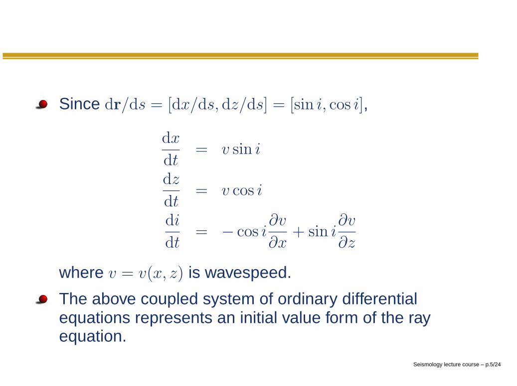
Since dr/ds = [dx/ds, dz/ds] = [sin i, cos i],

dx

dt= v sin i

dz

dt= v cos i

di

dt= − cos i

∂v

∂x+ sin i

∂v

∂z

where v = v(x, z) is wavespeed.

The above coupled system of ordinary differentialequations represents an initial value form of the rayequation.

Seismology lecture course – p.5/24

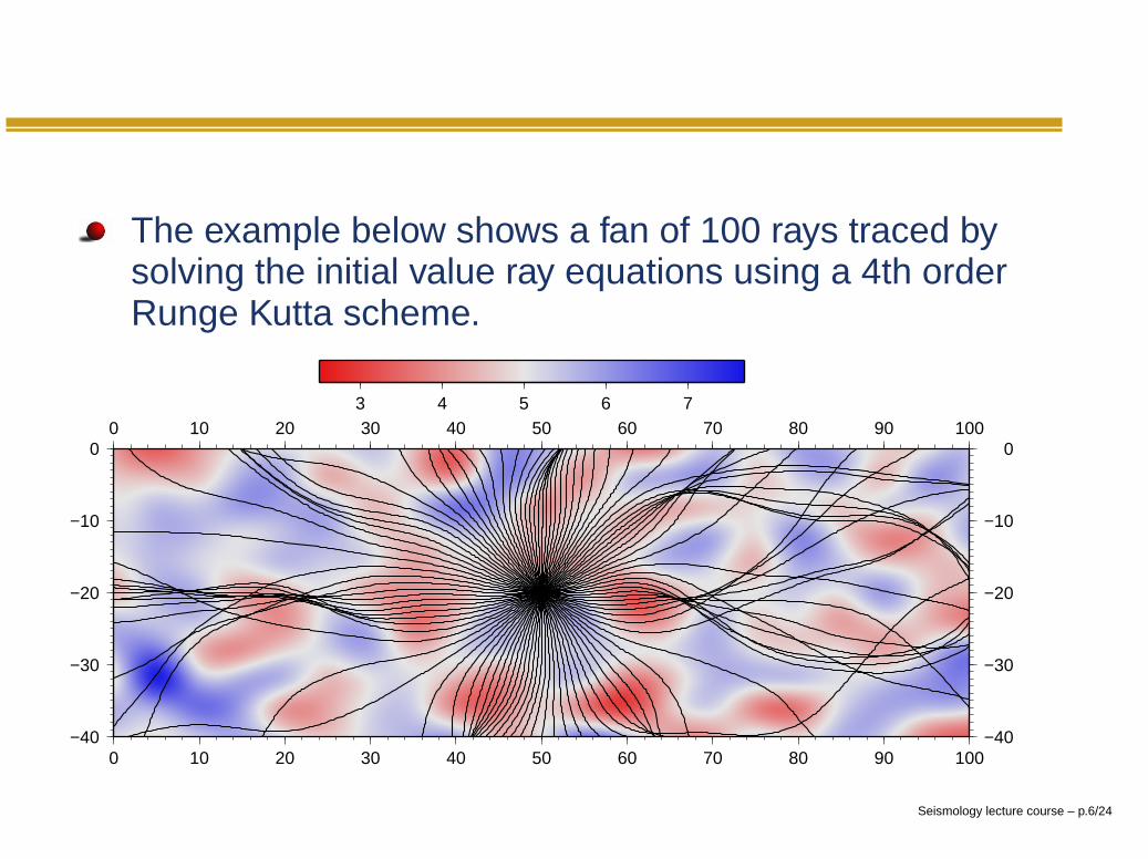
The example below shows a fan of 100 rays traced bysolving the initial value ray equations using a 4th orderRunge Kutta scheme.

−40

−30

−20

−10

0

−40

−30

−20

−10

0

0 10 20 30 40 50 60 70 80 90 100

0 10 20 30 40 50 60 70 80 90 1003 4 5 6 7

Seismology lecture course – p.6/24

Initial value ray tracing is powerful

Seismology lecture course – p.7/24

Shooting and bending methods

ShootingReceiver

Source

2

34

1 initial

final

x

z)x,z(v

BendingReceiver

Source

3

final

1 2

4

initial x

z)x,z(vSeismology lecture course – p.8/24

Ray tracingbecomes lessrobust as thecomplexity of themedium increases.

Can find a limitedclass of laterarrivals.

Reflection Paths

Refraction Paths

Seismology lecture course – p.9/24

The failure of ray tracing

Seismology lecture course – p.10/24

Eikonal solvers

Seek finitedifference solutionof eikonal equationthroughout agridded velocityfield (Vidale,1988,1990).

Very fast but firstarrival only.

Stability is anissue.

Upwind

Downwind

Seismology lecture course – p.11/24

Shortest Path Ray tracing (SPR)

A network or graph is formed by connectingneighbouring nodes with traveltime path segments(Moser, 1991).

Find path of minimum traveltime between source andreceiver through network using Dijkstra-like algorithms.

Not as fast aseikonal solvers,but tends to bemore stable.

Seismology lecture course – p.12/24

The Fast Marching Method (FMM)

FMM = grid based numerical scheme for tracking theevolution of monotonically advancing interfaces via FDsolution of the eikonal equation.

Only computes the first arrival in continuous media, butcombines unconditional stability and rapidcomputation.

⇒ It will always work regardless of the complexity ofthe medium. This is a very desirable feature.

First introduced by James Sethian (1996), whosubsequently applied it to a range of problems in thephysical sciences.

Seismology lecture course – p.13/24

Geodesics Robotic navigation

Medical imaging

Seismology lecture course – p.14/24

FMM in continuous media

Far pointsAlive points

DownwindUpwind

Close points

Narrow bandNarrow band sweepsthrough grid likea forest fire

Entropy condition:

it stays burntOnce a point burns,

Heap sort algorithm used to locate grid points innarrow band with minimum traveltime ⇒ O(M log M)operation count for FMM. Seismology lecture course – p.15/24

Updating grid points

The eikonal equation |∇xT | = s(x) is solved using an

entropy satisfying upwind scheme.

max(D−xa T,−D+x

b T, 0)2+

max(D−yc T,−D+y

d T, 0)2+

max(D−ze T,−D+z

f T, 0)2

1

2

ijk

= si,j,k

D−x1 Ti =

Ti − Ti−1

δxD−x

2 Ti =3Ti − 4Ti−1 + Ti−2

2δx

D1 or D2 are used depending on availability of upwindtraveltimes.

Seismology lecture course – p.16/24

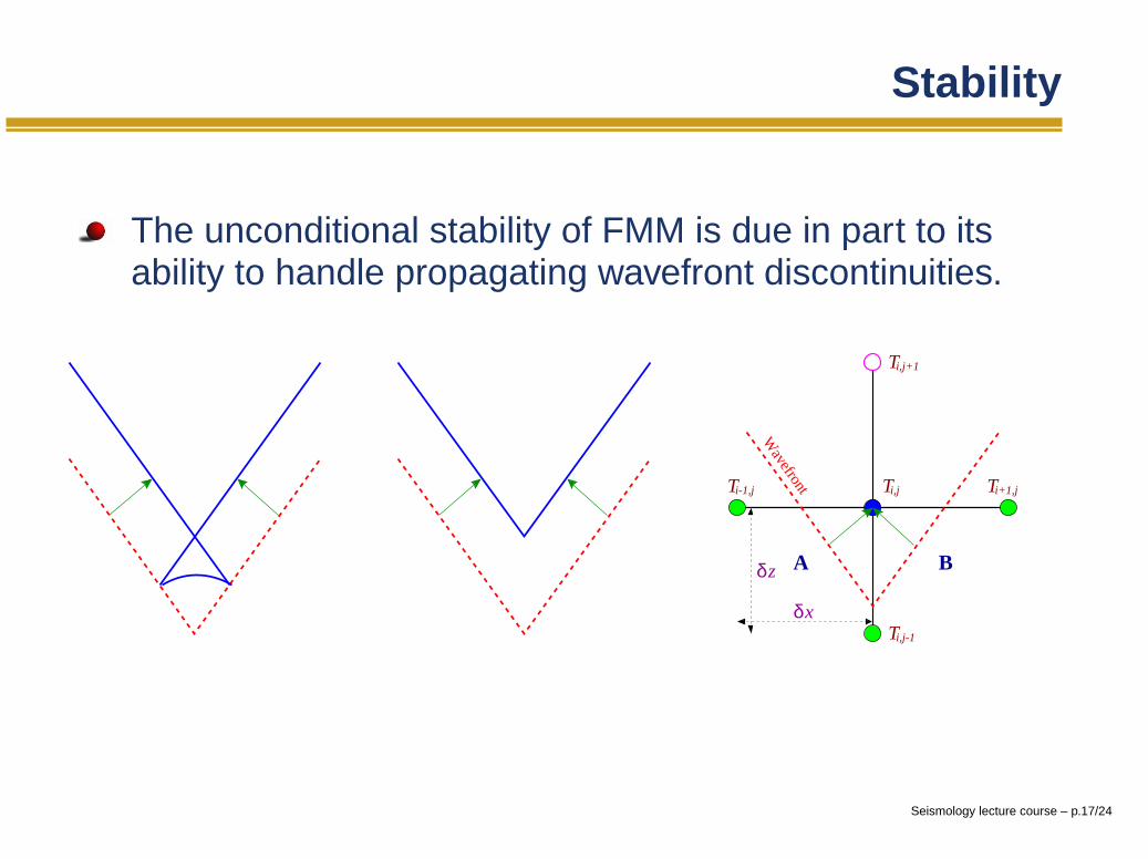
Stability

The unconditional stability of FMM is due in part to itsability to handle propagating wavefront discontinuities.

A B

WavefrontT Ti+1,jTi,j

i,j-1

i,j+1

δz

δxT

i-1,j

T

Seismology lecture course – p.17/24

Example

Wavefronts Rays

First order Second order

1000 m

500 m

250 m125 m

0.1 s

0.3 s

1.3 s5.8 s

T

0.3 s

1.2 s

5.3 s

0.1 s

125 m

250 m

500 m

1000 m= 12.98 sRMST= 12.98 sRMS

Seismology lecture course – p.18/24

Movie

Seismology lecture course – p.19/24

FMM in layered media

A locally irregular mesh of triangles is used to suturethe velocity nodes to the interface nodes.

A first-order entropy satisfying upwind scheme is usedto solve the eikonal equation within the irregular mesh.

Seismology lecture course – p.20/24

Example

Four branch multiplevelocity(km/s)

velocity(km/s)velocity(km/s)

41 2

2 3

3

1

Seismology lecture course – p.21/24

= 15.79 sRMST

125 m

250 m

0.2 s

0.8 s

2.9 s12.6 s

1000 m

500 m

velocity(km/s) velocity(km/s)

Snapshot of complete wavefield4

Seismology lecture course – p.22/24

Movies

Seismology lecture course – p.23/24

Seismology lecture course – p.24/24