seismic survey greenland 2013 - tgs 2013 (se...tgs february 2013 seismic survey greenland 2013...

TGS

February 2013

SEISMIC SURVEY GREENLAND 2013 Underwater sound propagation for South East Greenland off-shore seismic survey Mark Mikaelsen

NIRAS Greenland A/S Aaboulevarden 80 8000 Aarhus C, Denmark

Reg. No. 87672328 Denmark FRI, FIDIC www.niras.gl

P: +45 8732 3232 F: +45 8732 3200 E: [email protected]

D: +45 8732 5839 M: +45 3078 7543 E: [email protected]

PROJECT Seismic Survey Greenland 2013 Underwater sound propagation

Project No. 211914 Prepared by MAM Checked by SHKR Approved by ISA

Summary

This report presents underwater sound propagation modelling results for seismic survey activities in the offshore South East Greenland in summer and fall 2013, proposed by TGS. Seismic survey activities are performed using airgun arrays, that send high pres-sure waves toward the seabed, with the purpose of determining the geological properties of the different layers of the seabed. These high pressure waves cause sound pressure levels which may cause damage to nearby marine mam-mals and fish. Sound propagation modelling was performed to determine the sound pressure levels in the vicinity of, and inside the seismic survey area. The aim of the model-ling was to clarify the sound propagation in relation to nearby marine mammal protection zones. Modelling documented in this report, was performed using NIBAS and NISIM, both using a ray theory implementation called Bellhop. This implementation is range-, depth- and frequency-dependent, and takes the actual bathymetry, sound speed profiles, ice cover and seabed sediment type into account when calculat-ing the sound propagation. All these parameters were included in the modelling, with the exception of ice cover as it is expected that the survey area will be free of ice during the seismic survey period. Modelling was performed using available data for all the above mentioned pa-rameters for 10 source-receiver paths within the proposed seismic survey area. Results were presented as range-depth sound pressure level maps, for a repre-sentative number of frequency bands, along with a number of detailed range-range maps.

CONTENTS

Underwater sound propagation for seismic survey in South East Greenland – summer and fall 2013

www.niras.com

1 Introduction ................................................................................................ 1

2 Calculation area ......................................................................................... 3

2.1 Seismic survey area ................................................................................... 3

2.2 Modelling result presentation ...................................................................... 4

2.3 Modelling distance and frequency considerations ...................................... 4

2.4 Source-Receiver ......................................................................................... 6

3 Modelling Approach .................................................................................. 7

3.1 Airgun array ................................................................................................ 7

3.1.1 Source information ...................................................................... 7

3.1.2 Source pressure measurement procedure and implications .... 10

3.1.3 Calculation prerequisites for airgun array source level............. 11

3.2 Underwater sound propagation ................................................................ 12

3.2.1 Modelling methods and implementation ................................... 13

3.2.2 Environmental parameters ........................................................ 13

3.2.3 Environmental knowledge/Availability of data .......................... 14

3.2.4 Background noise ..................................................................... 16

3.3 Resume – chosen modelling parameters ................................................. 16

4 Results ...................................................................................................... 17

5 Discussion ................................................................................................ 18

Appendices ......................................................................................................... 20

1 Underwater sound propagation for seismic survey in South East Greenland – summer and fall 2013

www.niras.com

1 INTRODUCTION This report documents the underwater sound propagation modelling performed in connection with the EIA for TGS’ proposed seismic activities in the south east Greenland waters from June to October, 2013.

One of the requirements for the EIA is to calculate the extent of underwater sound exposure, as described in Kyhn et al., (2011). The newest version of the guidelines, the 3rd revision of December 2011, states:

“Requirement for modelling the extent of sound exposure at larger distances from the array, using adequate modelling of sound transmission, as well as con-firming this modelling by recordings made during the actual seismic survey.”

This requirement was added due to major concern for the effect of seismic activi-ties on marine mammals (especially whales) and fish (Kyhn et al., 2011)

Seismic surveys are performed using an airgun array that create high-pressure sound waves aimed towards the seabed, in order to analyse the geological properties of the seabed and the layers below.

This operation causes high sound pressure levels (SPL) in the surrounding wa-ters. Certain frequency components of the source signal can even be measured hundreds to thousands of km from the survey site.

There are many factors that influence how sound propagates within the ocean, among which surface shape, sound speed in the water column and the ocean depth are important factors. A description of these important factors, and how they are taken into consideration in the modelling, is available in chapter 3.

The purpose of the modelling described in this report is:

To use available knowledge about underwater sound propagation to obtain

an adequate estimate of the sound exposure extent in the South East

Greenland waters for seismic activities proposed by TGS. This, to enable

an educated assessment of the seismic surveys effect on marine mammals

and fish.


www.niras.com

Readers guide

This report consist of the following chapters:

Calculation area (2)

Provides a description of the seismic survey area. An overview map is provided in this chapter showing all modelling paths. Furthermore, gen-eral concerns and necessary considerations are addressed.

Modelling approach (3)

Describes the airgun array characteristics and the chosen underwater sound propagation model, along with a description of all important mod-elling parameters and their implementation in the model.

Results (4)

Describes the format of the modelling results. All results are presented in appendix using colour coded representations of sound pressure levels for the SPLpeak-peak and SPLrms90% modelling, and in sound exposure lev-els for the SEL modelling.

Discussion (5)

Discusses the results and what conclusions can be drawn, based on the modelling approach.

Appendices

Presents the results, along with examples of how the seabed type influ-ences the results. Also, an overview of the different ways to represent sound levels is given in the appendices.


www.niras.com

2 CALCULATION AREA This chapter provides an overview of the seismic survey area and the marine mammal protection zones in the vicinity. A method for representing the sound levels as a series of range-depth colour plots is given. Finally, a number of rep-resentative source-receiver paths are selected based on the survey area, the protection zones, and in order to accommodate the purpose of the modelling.

2.1 Seismic survey area The seismic survey in the south east waters of Greenland is proposed by TGS to be along the thin green lines shown on figure 1. On figure 1 the entire survey area, limited by the thick red line, covers over 400.000 km2. This introduces a challenge of how to model the sound levels for an area of this size.

To limit the calculation area, CMACS Ltd. chose to model throughout the entire area towards both shore and open sea, with special focus on the marine mam-mal protection zones in the south east waters.

The marine mammal protection zones relevant for this seismic survey are shown on figure 1.

Figure 1: Map of seismic survey lines and marine mammal protection zones. The thick red line indicate the survey area limit, while the thin green lines indicate the proposed survey lines. The grey lines show the marine mammal protection zones.

It is expected that the entire survey area will be free of ice during the seismic survey.


www.niras.com

2.2 Modelling result presentation With the 2011 revision of the guidelines (Kyhn et al., 2011), the requirement for more accurate sound pressure level (SPL) modelling was introduced. The guide-lines state:

“The model should be based on actual bathymetry, knowledge of sediment prop-erties (to the degree available) and realistic assumptions regarding vertical sound speed profiles and ice cover. Modelling should not be restricted to the surface layer but extend to at least 1000 m depth or the seabed. Horizontally, the model should extend to cover all areas exposed to levels likely to affect marine mammals.”

The requirement for use of actual bathymetry, sediment properties and ice cover, implies a need for a range-dependent modelling approach. The requirement for vertical sound speed profiles and a vertical modelling down to 1000 m depth or seabed, further implies a need for a depth-dependent model.

Thus, to accommodate the requirements, it is necessary to use a range- and depth-dependent modelling approach.

It was chosen to model the range- and depth-dependent sound pressure level (SPL) by choosing a representative number of range-depth SPL maps through-out the survey area. An example of such a map is given in figure 2 below, where, as a function of range and depth, the SPL is calculated with a given resolution (5 m vertically x 20 m horizontally in this example). The warmer the colour, the higher the SPL at that position, as shown by the scale on the right hand side.

Figure 2: Example of range-depth SPL map, where the SPL [dB re. 1 µPa] is shown using colours, warm colours being a high SPL, and cold colours represent a low SPL.

2.3 Modelling distance and frequency considerations Modelling distance

As described in Kyhn et al., (2011), underwater sound pressure measurements during previous seismic surveys have revealed that the airgun pulses can be observed at distances from the survey up to 3000 km. Ideally, underwater SPL modelling should thus extend to these ranges.


www.niras.com

Due to environmental uncertainties along with modelling technique limitations, SPL modelling at distances of several thousands of km is neither possible, nor reliable. The inherent issues will be explained further in chapter 3.

Based on preliminary modelling, using the same modelling technique and pa-rameters as described in chapter 3, it was concluded that the significant trans-mission loss occurs within the first 10 km of the source, and that harmful sound pressure levels are very unlikely to occur beyond this range.

Additionally, it was noticed that the sound transmission loss varies significantly with frequency over the first 50 km, and as such should be considered the mini-mum distance for modelling.

Based on the preliminary modelling, it was therefore chosen that all scenarios should extend to at least 50 km distance.

Frequency Range

Preliminary modelling show, that the loss of SPL over distance is very frequency dependent. The higher the frequency, the bigger the loss over distance.

Furthermore, as also explained in Caldwell & Dragoset, (2000), the source SPL decreases as the frequency is increased.

This suggests that in order to accurately model the SPL as a function of range and distance, it is necessary to model the SPL for different representative fre-quency bands. It was chosen to use the frequency bands given in table 1:

Frequency Band

Representative frequency

Frequency range of band

1 25 Hz 1 Hz – 37 Hz 2 50 Hz 37 Hz – 75 Hz 3 100 Hz 75 Hz – 150 Hz 4 200 Hz 150 Hz – 300 Hz 5 400 Hz 300 Hz – 500 Hz 6 600 Hz 500 Hz – 700 Hz 7 800 Hz 700 Hz – 900 Hz 8 1000 Hz 900 Hz – 1000 Hz 9 Broadband 1 Hz – 1000 Hz

Table 1: Frequency bands selected for SPL modelling. The frequency bands 1-8 are modelled, while band 9 is calculated from the results of band 1-8.


www.niras.com

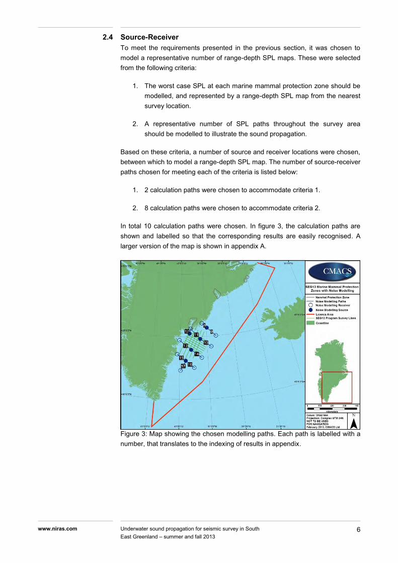
2.4 Source-Receiver To meet the requirements presented in the previous section, it was chosen to model a representative number of range-depth SPL maps. These were selected from the following criteria:

1. The worst case SPL at each marine mammal protection zone should be modelled, and represented by a range-depth SPL map from the nearest survey location.

2. A representative number of SPL paths throughout the survey area should be modelled to illustrate the sound propagation.

Based on these criteria, a number of source and receiver locations were chosen, between which to model a range-depth SPL map. The number of source-receiver paths chosen for meeting each of the criteria is listed below:

1. 2 calculation paths were chosen to accommodate criteria 1.

2. 8 calculation paths were chosen to accommodate criteria 2.

In total 10 calculation paths were chosen. In figure 3, the calculation paths are shown and labelled so that the corresponding results are easily recognised. A larger version of the map is shown in appendix A.

Figure 3: Map showing the chosen modelling paths. Each path is labelled with a number, that translates to the indexing of results in appendix.


www.niras.com

3 MODELLING APPROACH This chapter provides a description of the airgun array, based on data delivered by TGS. A suitable underwater sound propagation model is then chosen and the availability of the required parameters described in section 2.2 is investigated.

3.1 Airgun array The airgun array type and acoustic specifications was supplied by TGS. The source model used in the modelling reflects the supplied information. This sec-tion will only specify the parameters relevant for the underwater sound propaga-tion modelling.

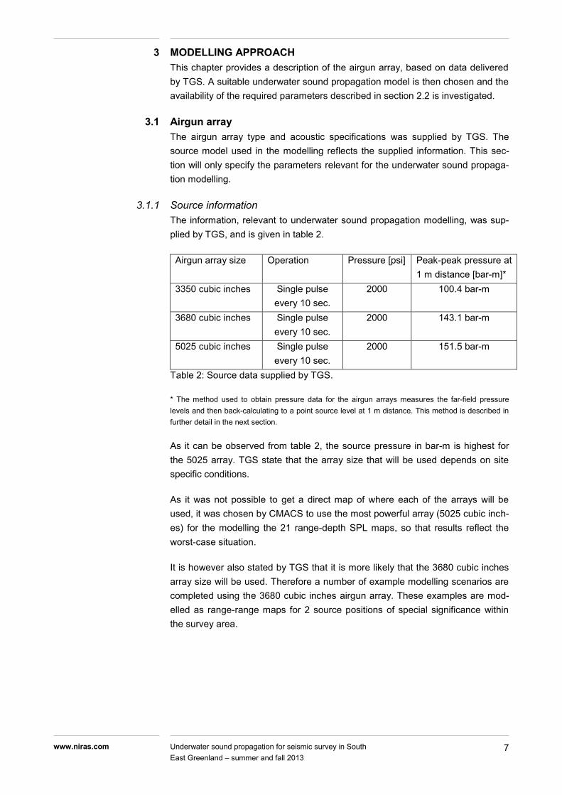
3.1.1 Source information The information, relevant to underwater sound propagation modelling, was sup-plied by TGS, and is given in table 2.

Airgun array size Operation Pressure [psi] Peak-peak pressure at 1 m distance [bar-m]*

3350 cubic inches Single pulse every 10 sec.

2000 100.4 bar-m


2000 143.1 bar-m


2000 151.5 bar-m

Table 2: Source data supplied by TGS.

* The method used to obtain pressure data for the airgun arrays measures the far-field pressure levels and then back-calculating to a point source level at 1 m distance. This method is described in further detail in the next section.

As it can be observed from table 2, the source pressure in bar-m is highest for the 5025 array. TGS state that the array size that will be used depends on site specific conditions.

As it was not possible to get a direct map of where each of the arrays will be used, it was chosen by CMACS to use the most powerful array (5025 cubic inch-es) for the modelling the 21 range-depth SPL maps, so that results reflect the worst-case situation.

It is however also stated by TGS that it is more likely that the 3680 cubic inches array size will be used. Therefore a number of example modelling scenarios are completed using the 3680 cubic inches airgun array. These examples are mod-elled as range-range maps for 2 source positions of special significance within the survey area.


www.niras.com

In addition to the data provided in table 2, the airgun array time-series for the airgun arrays were supplied by TGS. These are shown in figure 4 and figure 5.

Figure 4: Time-series for the 3350 and 5025 cubic inches airgun arrays.

Figure 5: Time-series for the 3680 cubic inches airgun array.


www.niras.com

Based on the time-series, the metrics given in table 3 were calculated by NIRAS. A short description of each metric is given in appendix I.

Source level for 3680 cubic inches airgun array SPLpeak-peak at 1 m distance [dB re. 1 µPa] 263 dB re. 1 µPa @ 1 m SPLzero-peak at 1 m distance [dB re. 1 µPa] 257 dB re. 1 µPa @ 1 m SPLrms90% at 1 m distance [dB re. 1 µPa rms] 238 dB re. 1 µPa rms @ 1 m Duration of RMS calculation [s] 0.29 s SEL at 1 m distance [dB re. 1 µPa2s] per pulse 234 dB re. 1 µPa2s @ 1 m Pulse duration [s] 0.4 s Source level for 5025 cubic inches airgun array SPLpeak-peak at 1 m distance [dB re. 1 µPa] 264 dB re. 1 µPa @ 1 m SPLzero-peak at 1 m distance [dB re. 1 µPa] 258 dB re. 1 µPa @ 1 m SPLrms90% at 1 m distance [dB re. 1 µPa rms] 241 dB re. 1 µPa rms @ 1 m Duration of RMS calculation [s] 0.25 s SEL at 1 m distance [dB re. 1 µPa2s] per pulse 235 dB re. 1 µPa2s @ 1 m Pulse duration [s] 0.4 s

Table 3: Source level for 3680 and 5025 cubic inches airgun array, calculated from time-series supplied by TGS.

The cumulative sound flux density [k Joule/m2 per pulse @ 1 m] was also calcu-lated for the 3680 and 5025 cubic inches arrays. The results are shown in figure 6 and figure 7.

Figure 6: Cumulative energy flux per pulse for airgun array 3680 cubic inches.


www.niras.com

Figure 7: Cumulative energy flux per pulse for airgun array 5025 cubic inches.

Based on the SPLpeak-peak for the airgun array and the frequency spectrum, the frequency bands from chapter 2.3 are revisited, with the purpose of determining the source SPLpeak-peak for the individual bands. See table 4.

3680 cubic inches

5025 cubic inches

Frequency band

Representative frequency

Frequency range of band

SPLpeak-peak

[dB re. 1 µPa @ 1 m]

SPLpeak-peak

[dB re. 1 µPa @ 1 m]

1 25 Hz 1 Hz – 37 Hz 248 dB 251 dB 2 50 Hz 37 Hz – 75 Hz 252 dB 252 dB 3 100 Hz 75 Hz – 150 Hz 248 dB 250 dB 4 200 Hz 150 Hz – 300 Hz 250 dB 249 dB 5 400 Hz 300 Hz – 500 Hz 244 dB 242 dB 6 600 Hz 500 Hz – 700 Hz 234 dB 232 dB 7 800 Hz 700 Hz – 900 Hz 228 dB 226 dB

8 1000 Hz 900 Hz – 1000 Hz

217 dB 213 dB

9 Broadband 1 Hz – 1000 Hz 263 dB 264 dB Table 4: SPLpeak-peak values for the different frequency bands for the 3680 and 5025 cubic inches airgun arrays.

3.1.2 Source pressure measurement procedure and implications In section 3.1.1, the known parameters for the airgun array were presented, and a number of additional source level representations were calculated.

The acoustic source level of the airgun array is based on a back-calculation from a far-field sound pressure measurement. This method of estimating the source level has certain limitations in terms of accuracy. This is explained in detail in Hannay et al., (2010) and Caldwell & Dragoset, (2000), and this section is there-fore written based on information presented there.


www.niras.com

The method of source level estimation by far-field measurement is commonly used to characterise the acoustic output level of airgun arrays, however it has certain disadvantages with regard to accuracy, especially for near-field distanc-es. These disadvantages are briefly described in the following, and the interested reader is referred to Caldwell & Dragoset, (2000) and Hannay et al., (2010) for further details.

In Hannay et al., (2010), the near-field inaccuracy of the back-calculation method is described as follows: “Far-field source levels do not apply in the near field of the array where pres-sures of the individual airguns do not add coherently; sound levels in the near field are, in fact, lower than would be calculated from far field estimates which assume coherent summation from all array elements” Another factor the far-field measurement does not account for, is the directivity of the airguns. As explained by Hannay et al., (2010), and Caldwell & Dragoset, (2000), far-field measurements of source levels, are done in the vertical direction relative to the airgun array, as this is the direction of interest for the seismic survey operations. The airgun pressure waves are focused downwards, and produce the highest pressure towards the seabed. According to Caldwell & Dragoset, (2000), the horizontal pressure can be up to 20 dB lower than the vertical pressure. For accurate near-field source level calculations, as well as accurate far-field sound level calculations in the horizontal direction, it is vital to consider parame-ters such as airgun directivity and individual airgun impulse responses to account for interference between the airguns.

3.1.3 Calculation prerequisites for airgun array source level Airgun directivity patterns and individual airgun impulse response data was not available for the chosen airgun array, and the calculations will therefore be based on the following worst-case scenario assumptions.

1. The directivity of the airgun array is assumed omnidirectional. That is, the horizontal sound pressure is assumed equal to the vertical.

2. The airgun array is considered a point source. These assumptions will result in calculated sound pressure levels being consid-erably higher than the actual levels. The highest deviations between the actual sound pressure levels and the calculated, are expected to be in the near-field, (D. Hannay et al. 2010), (Caldwell & Dragoset, 2000).


www.niras.com

3.2 Underwater sound propagation This section is written based on Jensen et al., (2011) chapter 1 and chapter 3 as well as Porter, (2011). This chapter will give a brief introduction to sound propa-gation in oceans, and the interested reader is referred to Jensen et al., (2011) chapter 1, for a more detailed and thorough explanation of underwater sound propagation theory.

In the ocean, the sound pressure level generally decreases with increasing dis-tance from the source. However, many parameters influence the propagation and makes it a complex process.

The speed of sound in the ocean, and thus the sound propagation, is a function of first and foremost pressure, salinity and temperature, all of which are depend-ent on depth and the climate above the ocean and as such are very location dependent.

The theory behind the sound propagation is not the topic of this report, however it is worth mentioning one aspect of the sound speed profile importance.

Snell’s law states that:

Where is the ray angle, and c is the speed of sound [m/s], thus implying that sound bends toward regions of low sound speed (Jensen et al. (2011). The im-plications for sound in water are, that sound that enters a low velocity layer in the water column can get trapped there. This results in the sound being able to travel far with very low sound transmission loss.

The physical properties of the sea surface and the seabed further affect the sound propagation by reflecting, absorbing and scattering the sound waves. Roughness, density and media sound speed are among the surface/seabed properties that define how the sound propagation is affected by the boundaries.

The listed parameters are merely the most important ones. Other parameters include volume attenuation of the water column, which is explained further in Jensen et al., (2011).


www.niras.com

3.2.1 Modelling methods and implementation There are different approaches to include all necessary parameters into an un-derwater sound propagation model, based on different physics models. The most common are:

- Ray methods (range-dependent)

- Parabolic equation (range-dependent)

- Wavenumber integration techniques (range-independent)

- Normal modes (range-independent)

For the interested reader, the theory behind the different models is explained in detail in Jensen et al., (2011).

Range-independent models are not considered further, as those do not allow changes in bathymetry and sound speed profiles over distance. Only ray method and parabolic equation models are therefore of interest.

Michael B. Porter, president of HLS Research, and one of the co-authors of Jen-sen et al. (2011), developed a ray method implementation called Bellhop.

Mike Collins from the US Naval Research Laboratory developed a parabolic equation implementation called RAM (Range-dependent Acoustic Model).

These implementations have proven to produce results very similar to other techniques, such as normal mode implementations [Porter, M.B., 2011].

Bellhop is very thoroughly documented, and is still being updated whenever new knowledge of underwater sound propagation is discovered. It is also a very com-putationally efficient implementation.

Niras has two programs for underwater noise propagation modeling.

NIBAS, which is built on the Bellhop implementation of ray/Gaussian beam theo-ry. NIBAS produces range-depth maps and was the program of choice for mod-eling the 21 source-receiver range-depth maps.

NISIM, which is built on both Bellhop and RAM, and then choses the best model for each specific scenario. NISIM produces range-range maps and was the pro-gram of choice for the 2 examples using the 3680 cubic inches array size. NISIM is a program made by Michael B. Porter and Laurel Henderson at HLS Re-search.

3.2.2 Environmental parameters As previously described, there are many parameters that influence the sound propagation in the ocean.


www.niras.com

Guideline requirements for modelling parameters to be included As cited in section 2.2, (Kyhn et al., 2011) states that the model should include the following parameters:

Actual bathymetry Realistic assumptions of the sound speed profile Sediment properties (to the degree available) Realistic assumptions of ice cover All frequencies relevant for biological species

Parameters that Bellhop and RAM support Both implementations allow for input of the following range dependent parame-ters:

Sound speed profile (dependent on temperature, salinity and pressure) Bathymetry Altimetry (surface thickness, in case of ice cover)

Furthermore, it allows for the following range independent inputs:

Physical parameters for the surface (used for ice cover) Physical parameters for the seabed (sediment properties)

They further allow for performing calculations for all frequencies. As shown, both implementations support all required inputs, and the limitation, if any, will therefore be the availability of such input data. The choice between RAM and Bellhop for the NISIM calculations depend on the site specific condi-tions.

3.2.3 Environmental knowledge/Availability of data The availability of each required parameter is discussed in the following. NIBAS and NISIM use different databases, as indicated in the sections below.

Range dependent bathymetry (Seabed profile) Several databases for ocean depth exist, and are available online. One of these, based on quality controlled ship depth soundings and satellite gravity data, is the General Bathymetric Chart of the Oceans (GEBCO), (www.gebco.net, 2011). GEBCO is a one minute resolution map of the ocean depth worldwide. NIBAS uses GEBCO for supplying bathymetry data. Another bathymetry database is ETOPO-1 by the National Geophysical Data Center under the American NOAA (Amante, C., 2009). ETOPO-1 is a 1 arc-minute model and consist of data from a number of regional and global data sets. NISIM uses ETOPO-1 by default.

http://www.gebco.net/


www.niras.com

Range dependent sound speed profile (SSP) As for the bathymetry, several databases for sound speed profiles, exist. One of these, that include worldwide coverage, is the World Ocean Atlas from 2009 (WOA09), (Locarnini, R. A. et al., 2010), (Antonov, J. I. et al., 2010). It is an ob-jectively analysed 1° resolution database including more than 20 parameters, the interesting of which are temperature, pressure and salinity, all given in annual, seasonal and monthly averages, based on historical data. Since the sound speed profile is a function of temperature, pressure and salinity, this database can be used to calculate the sound speed profile. Both NIBAS and NISIM use WOA09 due to the availability of all relevant parame-ters for calculating the sound speed profile, and due to being a widely used and maintained database. Sediment properties

To determine the sediment properties for the seabed, the GEUS maps were studied. Unfortunately, most of the seabed in the survey area is labelled “Little known basin with thick sedimentary succession” and “Area underlain by conti-nental crust”. However a database called CRUST5.1 (Mooney, W.D. et al., 1998), provided rough estimates of the sound velocity in the seabed top layer for the survey area. Based on the observed worst-case sound velocity in the survey area, the corresponding sediment type was determined from Jensen et al., (2011).

The sediment corresponding to this sound velocity is acoustically similar to the Chalk sediment type in Jensen et al., (2011), which was therefore chosen for sound propagation modeling in south east Greenland. This sediment type is hard and reflective.

The sediment data listed in table 7 was used in the model:

Sediment cp [m/s] rp [kg/m3] αp [dB/lp]

Chalk 2400 2200 0.2 Table 7: Sediment acoustic properties (Jensen et al., 2011).

NIBAS used the above information as input for sediment type.

Another database for sediment information is the dbSEABED by Institute for Arctic and Alpine Research, University of Colorado at Boulder (dbSEABED, 2008). NISIM uses dbSEABED for determining the sediment type.


www.niras.com

Ice cover

A major uncertainty is the ice cover. Since this report models what will be the conditions in a future time, the ice cover is unknown. It is however, from historical data known that the entire survey area planned for 2013 as indicated by the green lines on figure 1 will be free of ice. It was therefore chosen not to model ice-cover for this seismic survey.

Volume Attenuation in the water column

Another parameter that has influence on especially the high frequency transmis-sion loss over distance is the volume attenuation, defined as an absorption coef-ficient reliant on chemical conditions of the water column. This parameter has been approximated by:

Where f is the frequency of the wave in kHz (Jensen et al., 2011).

3.2.4 Background noise There will be several sources of noise not included in the underwater sound propagation modelling. These are:

- Any biological sources, such as shrimps, whales and other marine mammals.

- Noise from ships, both those dragging the airgun array, follower ships etc.

3.3 Resume – chosen modelling parameters Due to unknown conditions in survey area, and unknown source characteristics, the following parameters were chosen for underwater sound propagation model-ling. The reader is referred to the respective previous sections for explanations on choice of parameters.

Range dependent sound speed profiles from WOA09

Range dependent bathymetry data from GEBCO database for NIBAS modelling, while ETOPO-1 is used for NISIM modelling.

Seabed sediment type was chosen to be a hard reflective surface, due to information from CRUST 5.1 database. A hard reflective surface will present the absolute worst case scenario.

Surface was chosen to be free of ice, based on historical data.


www.niras.com

The source is modelled as an omnidirectional point source. This will re-sult in the worst case results, and as a result of this, actual sound pres-sure levels are expected to be significantly lower than the modelled lev-els.

For the NIBAS range-depth modelling, it was chosen to model the un-derwater sound pressure levels in 8 representative frequency bands within the range 1 Hz – 1000 Hz, due to being the frequency area with the lowest transmission loss, and the highest source SPL.

For the NISIM range-range modelling, it was chosen to model only broadband levels (corresponding band 9 in table 1), in 4 depths below the water surface; 10 m, 50 m, 250 m and 750 m. NISIM modelling was chosen to present results in both SEL, SPLrms90% and SPLpeak-peak.

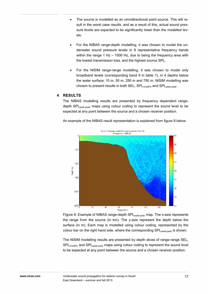
4 RESULTS The NIBAS modelling results are presented by frequency dependent range-depth SPLpeak-peak maps using colour coding to represent the sound level to be expected at any point between the source and a chosen receiver position.

An example of the NIBAS result representation is explained from figure 8 below.

Figure 8: Example of NIBAS range-depth SPLpeak-peak map. The x-axis represents the range from the source (in km). The y-axis represent the depth below the surface (in m). Each map is modelled using colour coding, represented by the colour bar on the right hand side, where the corresponding SPLpeak-peak is shown.

The NISIM modelling results are presented by depth slices of range-range SEL, SPLrms90% and SPLpeak-peak maps using colour coding to represent the sound level to be expected at any point between the source and a chosen receiver position.


www.niras.com

An example of the NISIM result representation is explained from figure 9 below.

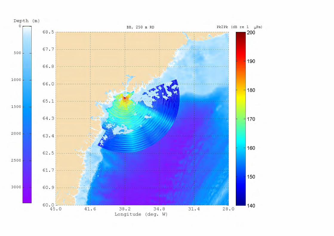
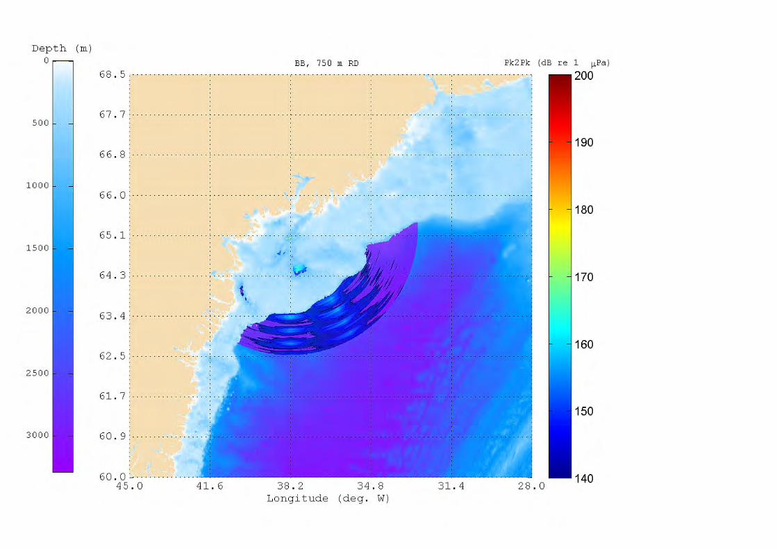
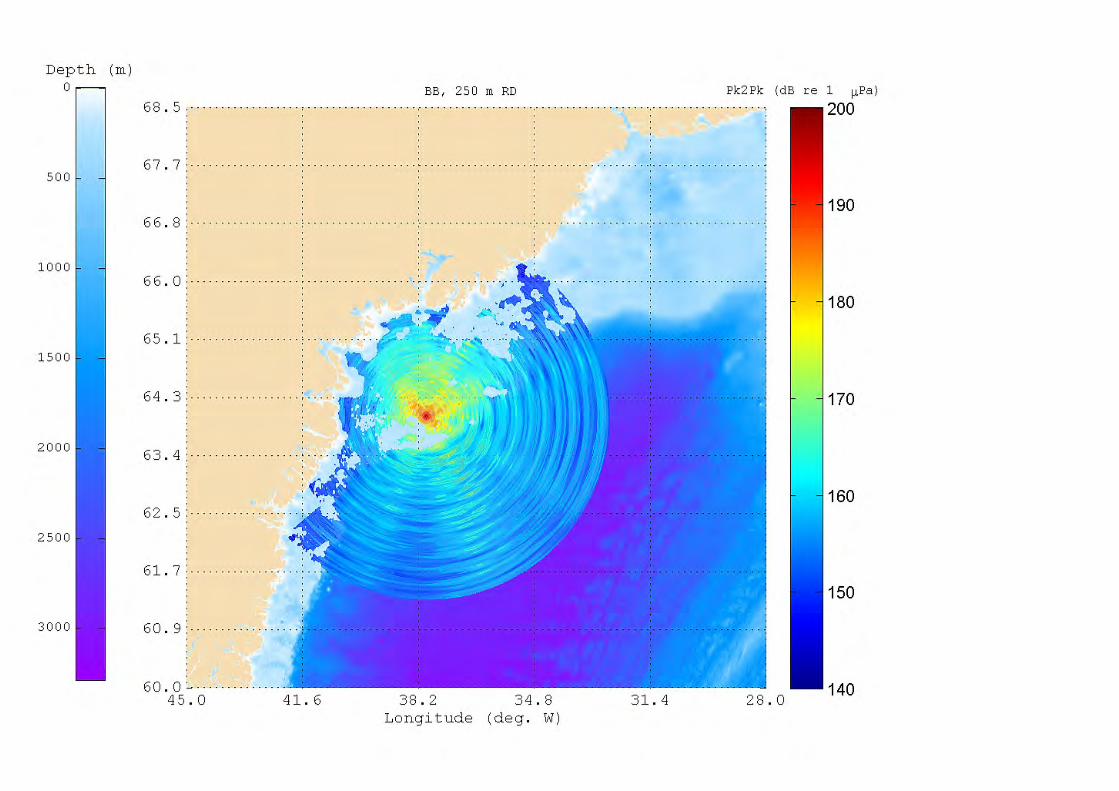
Figure 9: Example of NISIM range-range SPLpeak-peak map at a depth of 10 m below surface. Results are presented using colour coding to represent the sound pressure level, represented by the colour bar on the right hand side, where the corresponding SPLpeak-peak is shown. NISIM results are shown on a geographical map so that the SPLpeak-peak at any coordinate, at the current depth can be seen directly. Purple areas within the modelled range indicate sound levels below the set scale, in this example 140 dB.

5 DISCUSSION The underwater sound propagation modelling was based on certain assumptions regarding seabed sediment type and airgun characteristics. This led to a model assuming worst-case conditions for all of the parameters.

In order to more accurately model underwater sound propagation in the future, it is necessary to have:

- More accurate knowledge of the seabed sediment layers and acoustic properties would allow for more precise bottom loss modelling.

- Knowledge of frequency dependent airgun directivity data along with near-field single airgun impulse response measurements would allow for a more accurate near-field modelling.


www.niras.com

References

Antonov, J. I., D. Seidov, T. P. Boyer, R. A. Locarnini, A. V. Mishonov, and H. E. Garcia, (2010). World Ocean Atlas 2009 Volume 2: Salinity. S. Levitus, Ed., NOAA Atlas NESDIS 69, U.S. Government Printing Office, Washington, D.C., 184 pp.

Caldwell, J., Dragoset, W. (2000): A brief overview of seismic air-gun arrays, The Leading Edge, Aug. 2000, pages. 898-902.

dbSEABED, (2008), Seabed from NCEAS conversion of dbSEABED into ‚hard and ‚soft bottom types, Halpern et al., Science v. 15, pp. 948-052, 2008;

ETOPO1: Amante, C. and B. W. Eakins, (2009), ETOPO1 1 Arc-Minute Global Relief Model: Procedures, Data Sources and Analysis. NOAA Tech-nical Memorandum NESDIS NGDC-24, 19 pp, March 2009.

Hannay, D., Racca, R., MacGillivray, A., (2010), Model Based Assessment Of Underwater Noise from an Airgun Array Soft-Start Operation, JASCO Ap-plied Sciences, Oct. 2010.

Jensen, F.B. (1982), Numerical models of sound propagation in real oceans. Proc MTS / IEEE Ocean 82 Conf., p. 147-55

Jensen, F.B., Kuperman, W.A., Porter, M.B., Schmidt, H., (2011), Computa-tional Ocean Acoustics, 2nd edition, Springer, 2011.

Kyhn, L.A., Boertmann, D., Tougaard, J., Johansen, K., Mosbech, A., (2011): Guidelines to environmental impact assessment of seismic activities in Greenland Waters, 3rd revised edition, Danish Center for Environment and Energy, Dec. 2011.

Locarnini, R. A., A. V. Mishonov, J. I. Antonov, T. P. Boyer, and H. E. Garcia, (2010). World Ocean Atlas 2009, Volume 1:Temperature. S. Levitus, Ed., NOAA Atlas NESDIS 68, U.S. Government Printing Office, Washington, D.C., 184 pp.

Mooney, W.D., Laske, G., Masters, G., (1998), CRUST5.1: A global crustal model at 5°x5°., J. Geophys. Res., 103, 727-747.

Porter, M.B., (2011), The BELLHOP Manual and User’s Guide: PRELIMINARY DRAFT, Heat, Light, and Sound Research, Inc., La Jolla, CA, USA, Jan. 2011.

The GEBCO One Minute Grid, version 2.0, www.gebco.net, 2011

http://www.gebco.net/


www.niras.com

APPENDICES The following appendices are included in this report:

A. Overview map of modelling paths.

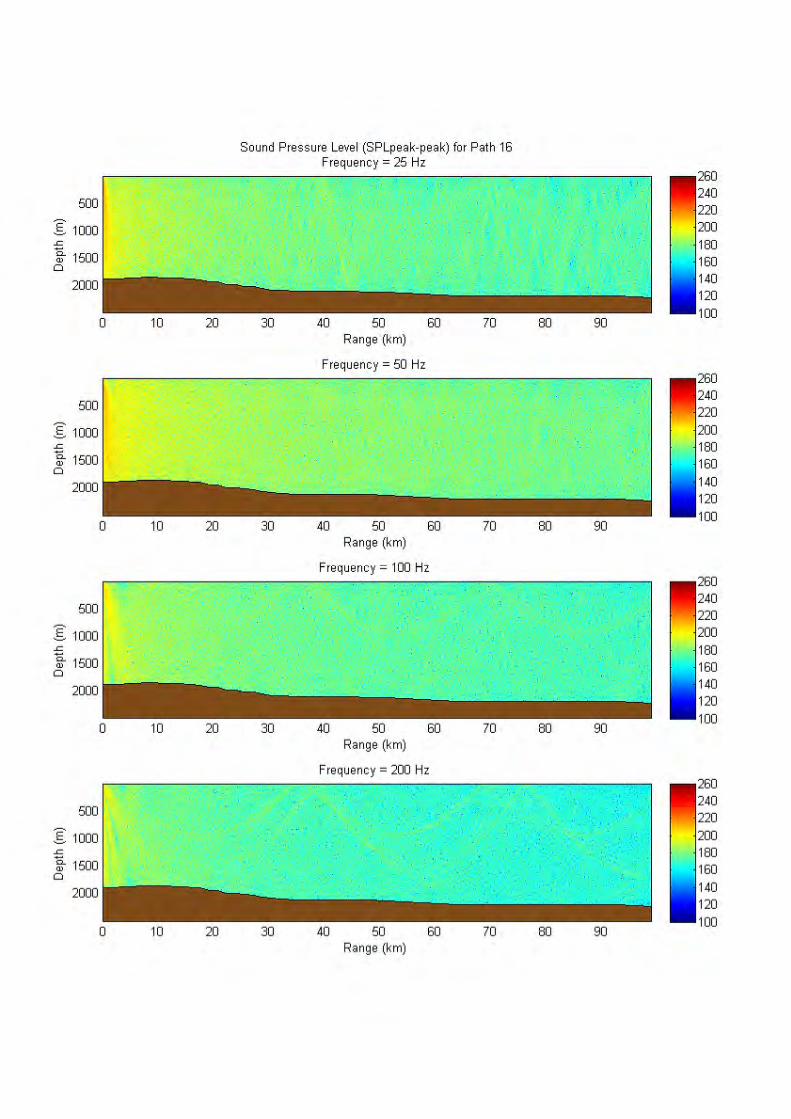
B. Path 8 – 17 range-depth narrowband SPLpeak-peak results.

C. Path 8 – 17 range-depth broadband SPLpeak-peak results.

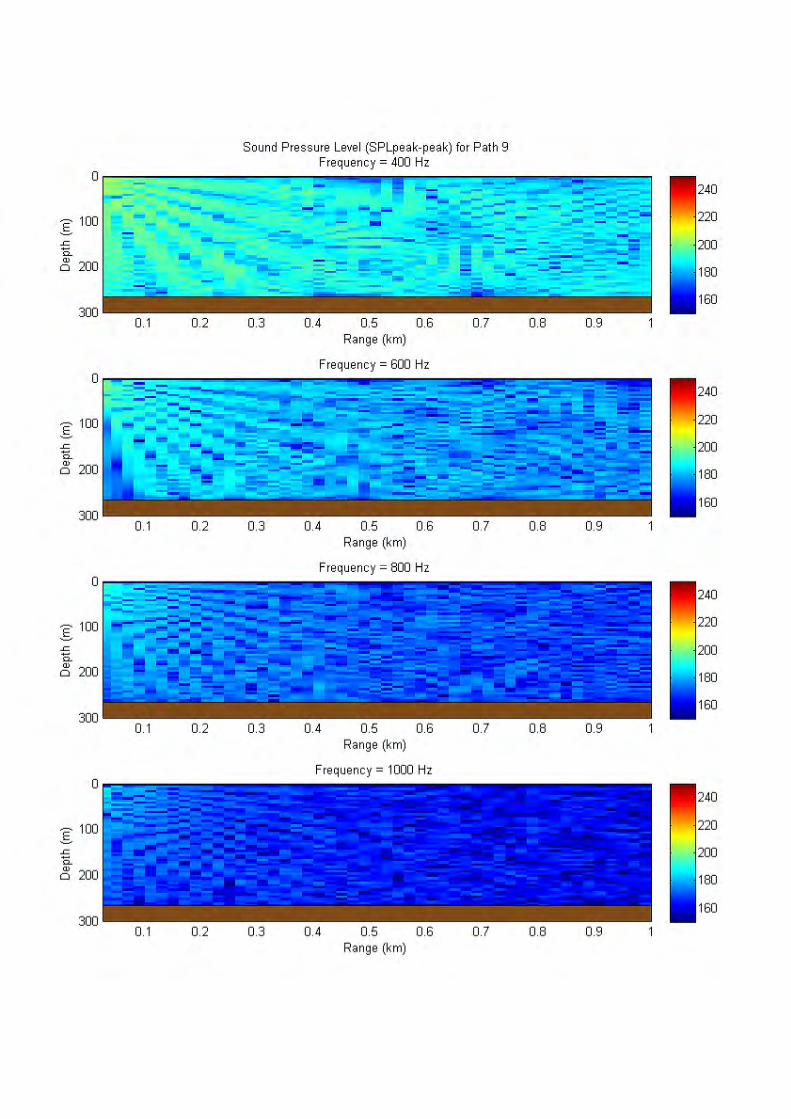
D. Path 9 zoomed in on the first 1 km

E. Path 9 zoomed in on the first 10 km

F. Source location 1 range-range broadband SPLpeak-peak, SPLrms90%, SEL results.

G. Source location 2 range-range broadband SPLpeak-peak, SPLrms90%, SEL results.

H. 240 dB & 220 dB SPLpeak-peak distance from source for broadband SPLpeak-peak results.

I. Sound metrics

240 dB re. 1 µPa 220 dB re. 1 µPa

Path 8 75 m 900 m

Path 9 50 m 600 m

Path 10 50 m 500 m

Path 11 75 m 800 m

Path 12 75 m 1000 m

Path 13 75 m 900 m

Path 14 50 m 600 m

Path 15 50 m 350 m

Path 16 50 m 300 m

Path 17 50 m 350 m

Appendix H:

240 dB & 220 dB SPLpeak-peak distance from source for broadband results.

The table below shows the distance from source for each path, at which the

broadband SPLpeak-peak drops below the 240 dB and 220 dB limits.

Path Distance from source where

broadband SPLpeak-peak drops below:

APPENDIX I: SOUND METRICS

Underwater sound levels are measured in dB re. 1 µPa. Different methods of representing the sound level exist to characterize the intensity, exposure level, or even max levels. Depending on the intended use of the results, and the type of source, it can be useful to use one sound level representation over another. For impulsive sound sources, such as an airgun array, the four most commonly used ones are:

1. The sound pressure level peak-peak (SPLpeak-peak) and zero-peak (SPLzero-peak)

2. The root-mean-square sound pressure level (SPL90%rms)

3. The sound exposure level (SEL)

4. The cumulative energy flux

These four metrics are briefly explained in the following

SPLzero-peak and SPLpeak-peak

The SPLzero-peak is the maximum instantaneous sound pressure level of an im-pulse p(t), given by:

| )|)

The closely related SPLpeak-peak is the maximum difference in sound pressure level of an impulse p(t), given by:

( ( )) | ( ))|)

which is also the metric used for the modelling in this project.

2

SPL90%rms

The SPL90%rms is the root-mean-square pressure level over a time window, T, containing the impulse p(t):

(

∫ )

)

The SPL90%rms is defined as the mean value of a pulse with the time window T containing “90% of the pulse energy” as described in [Malme et al. 1986]. As a result of dividing by the time window T in the equation, pulses with the energy spread out over a long duration will have a lower SPL90%rms than a short duration pulse with the same total energy. It is therefore a useful metric to describe the impulsivity of a source.

SEL

The SEL, also known as the sound exposure level is defined as the time-integral of the square pressure over a time window T covering the entire pulse duration, and is given by:

(∫ )

)

Cumulative Energy Flux

The cumulative energy flux is a standard measure for airgun arrays. The power spectrum is integrated, and the result is shown with increasing frequency.

seismic survey greenland 2013 - tgs 2013 (se...tgs february 2013 seismic survey greenland 2013...

Documents