seismic refraction and electrical resistivity tests for
TRANSCRIPT

SEISMIC REFRACTION AND ELECTRICAL RESISTIVITY TESTS FOR
FRACTURE INDUCED ANISOTROPY IN A MOUNTAIN WATERSHED
by
Aída Mendieta
A thesis
submitted in partial fulfillment
of the requirements for the degree of
Master of Science in Geophysics
Boise State University
December 2017

© 2017
Aída Mendieta
ALL RIGHTS RESERVED

BOISE STATE UNIVERSITY GRADUATE COLLEGE
DEFENSE COMMITTEE AND FINAL READING APPROVALS
of the thesis submitted by
Aída Mendieta
Thesis Title: Seismic Refraction and Electrical Resistivity Tests for Fracture Induced
Anisotropy in a Mountain Watershed
Date of Final Oral Examination: 27 October 2017
The following individuals read and discussed the thesis submitted by student Aída
Mendieta, and they evaluated her presentation and response to questions during the final
oral examination. They found that the student passed the final oral examination.
John Bradford, Ph.D. Chair, Supervisory Committee
Lee M. Liberty, M.S. Member, Supervisory Committee
James P. McNamara, Ph.D. Member, Supervisory Committee
The final reading approval of the thesis was granted by John Bradford, Ph.D., Chair of the
Supervisory Committee. The thesis was approved by the Graduate College.

iv
DEDICATION
This thesis is dedicated to my nephews: Gabriel and Julio Mendieta.
v
ACKNOWLEDGEMENTS
As usual, it is impossible to thank everyone who has helped even in the littlest of
bits in the completion of this thesis, but I’ll try! Beginning with my advisor John Bradford,
for all the never ending patience, and continued guidance to help me become a better
researcher. Lee Liberty and Jim McNamara for guiding me through this research, and
allowing me to ask questions whenever. For the mentoring received from Travis Nielson
and Pamela Aishlin, your help was invaluable for this research. I also want to thank
Professor Dylan Mikesell for teaching me how to use PRONTO.
Every single person who helped me with the data collection: Travis Nielson, Lucy
Gelb, Andy Karlson, Andrew Poley, Joel Góngora, Diego Domenzain, Rebekah Lee,
Marlon Ramos, Zongbo Xu, Tom Harper, Hamid Dashti, Nayani Ilangakoon, Becca Garst,
Tate Meehan, Andrew Gaze, Tom Van Der Weide, Binbin Mi, Chao Shen, Thomas
Otheim, Hugo Ortiz, Nicole Clizzie, James Ford, and Dominic Filiano.
For all the moral support from friends back home: Irving, William, Miguel, and
Débora. For all the support given to me by my aunts and uncles, specially: Margarita
Carías, Aurelia Poulsen, Francisco Mendieta, and Aída Mendieta. For all the moral support
received from home, by my mother, sisters, and nephews: Lorena Tenorio, Aleja Mendieta,
Natalia Mendieta, Julio Mendieta and Gabriel Mendieta.
I am grateful for the funding given to me by Fulbright and the Geological Society
of America, allowing me to do this research.

vi
ABSTRACT
The critical zone (CZ) is the earth’s layer where water, air, rock, and life meet. It
is the zone with which humans interact most. The National Research council (2001)
defines the CZ as a “heterogeneous, near surface environment in which complex
interactions involving rock, soil, water, air, and living organisms regulate the natural
habitat and determine the availability of life sustaining resources”. The CZ may extend
roughly from the top of the vegetation canopy to the deepest part of the rock column
where meteoric water circulates – this is often in the 10 – 30 m range. The upper 1-2 m of
the CZ, the most weathered portion of the CZ depth profile, can be reached via soil pits
or cores enabling detailed characterization. Weathering is the process in which a parent
rock decays into mobile soil, through mechanical breakdown and chemical weakening.
The maximum depth at which both, mechanical and chemical processes are present is
referred to as weathering depth. Below 2 m, characterizing the CZ is a challenge because
of the expense and logistical challenge of drilling boreholes, particularly in rugged,
mountainous terrain. Geophysical methods are increasingly being used to probe deeper
into the CZ and have proven to be a powerful tool. Fully characterizing the deep CZ is
made even more challenging when fractures are present. Fractures may have a
preferential orientation according to the local stress field which leads to both geophysical
and hydraulic anisotropy. Because fractures can be hydraulically active, understanding
fracture induced anisotropy retrieves information on the preferential distribution of water
vii
pathways in the subsurface. To test our ability to detect and characterize systems of deep
CZ fractures with preferred orientation in a mountain watershed, I conducted a series of
multi-azimuthal 2D electrical resistivity tomography and 2D seismic refraction surveys. I
utilized the Dry Creek Experimental Watershed (DCEW) as a field laboratory – a
previous outcrop study mapped fracture orientations throughout the watershed. I
collected data, at three different sites, near or within the DCEW. For the anisotropy and
fracture density case, I estimated fracture density as a function of depth at all sites, and
determine that the depth at which most fractures close ranges from 13-27 m depth. I
found significant P-wave anisotropy throughout the watershed with maximum values of
28%. Additionally, my results indicate that anisotropy continues to much greater depths. I
infer that the observed geophysical anisotropy likely correlates with significant hydraulic
anisotropy and has an important impact on deep water circulation in the DCEW.
Additionally, I show that attempts to characterize this system with single azimuth data
and an assumption of isotropy will lead to erroneous results – at my sites the error in
estimated fracture density could be as high as 0.24. I conclude that geophysical
investigations in similar terrains need to test for anisotropy and use appropriate models,
particularly if the objective is quantitative estimation of hydraulic or other physical
properties. General observations of the CZ were that weathering depth increased with
decreasing elevations – this has been observed at other sites and is likely due to increased
chemical reactivity at higher temperatures. At the low elevation site I observe a depth to
bedrock at approximately 29 m depth, at the mid-elevation site I observe a depth to
bedrock of approximately 23 m depth, at the high elevation site, I observe a depth to
bedrock as little 5 m depth. I observed a significant increase in weathering depth on

viii
northwest facing aspects and speculate that this is a combination of lower evaporation
rates, slow steady delivery of snow melt waters into the subsurface and the positive
feedback of increased vegetation and root enhanced weathering.

ix
TABLE OF CONTENTS
DEDICATION ................................................................................................................... iv
ACKNOWLEDGEMENTS .................................................................................................v
ABSTRACT ....................................................................................................................... vi
LIST OF TABLES ............................................................................................................ xii
LIST OF FIGURES ......................................................................................................... xiii
LIST OF ABBREVIATIONS ............................................................................................xv
CHAPTER ONE: INTRODUCTION ..................................................................................1
1.1 Importance .........................................................................................................1
1.2 Research Hypothesis ..........................................................................................5
1.3 Description of research sites ..............................................................................6
1.2.1 Lower Weather .................................................................................8
1.2.2 Treeline.............................................................................................9
1.2.3 Bogus Basin....................................................................................10
1.4 Development of research .................................................................................10
CHAPTER TWO: SEISMIC REFRACTION ...................................................................12
2.1 Seismic methods ..............................................................................................12
2.1.1 Seismic refraction .............................................................................12
2.1.2 Seismic anisotropy ............................................................................12
2.1.3 Fracture density calculation ..............................................................16

x
2.1.4 Data collection ..................................................................................17
2.1.5 Data processing .................................................................................19
2.2 Seismic refraction results .................................................................................20
2.2.1 Lower Weather results ......................................................................20
2.2.2 Treeline results ..................................................................................26
2.2.3 Bogus Basin results ...........................................................................35
2.3 Seismic refraction discussion .....................................................................43
2.4 Seismic refraction conclusions ........................................................................50
CHAPTER THREE: ELECTRICAL RESISTIVITY TOMOGRAPHY ..........................52
3.1 Electrical resistivity methods ...........................................................................52
3.1.1 Electrical resistivity tomography ......................................................52
3.1.2 Electrical anisotropy .........................................................................52
3.1.3 Electrical resistivity data collection ..................................................53
3.1.4 Electrical resistivity data processing .................................................55
3.2 Electrical resistivity results ..............................................................................56
3.2.1 Lower Weather results ......................................................................56
3.2.2 Treeline results ..................................................................................59
3.3 Electrical resistivity discussion ........................................................................63
3.4 Electrical resistivity conclusions......................................................................63
CHAPTER FOUR: WEATHERING DEPTH ...................................................................64
4.1 Weathering depth results ..................................................................................64
4.1.1 Weathering depth as a function of elevation .....................................64
4.1.2 Weathering depth per aspect per site ................................................65

xi
4.2 Weathering depth discussion ...........................................................................69
4.3 Weathering depth conclusions .........................................................................73
CHAPTER FIVE: CONCLUSIONS AND RECOMMENDATIONS ..............................74
REFERENCES ..................................................................................................................77
APPENDIX ........................................................................................................................85

xii
LIST OF TABLES
Table 1: Correlation between granite weathering states and geophysical parameters. ......21
Table 2: Treeline NR anisotropy values. ...........................................................................34
Table 3: Treeline SR anisotropy values. ............................................................................34
Table 4: Bogus Basin anisotropy values. ...........................................................................40
Table 5: Mean depth to bedrock at the Treeline site. .........................................................64
Table 6: Mean depth to bedrock at the Bogus Basin site. ..................................................65
Table 7: Weathering layer thicknesses for the Lower weather site.. .................................66
Table 8: Weathering layer thicknesses for the NR at Treeline. .........................................67
Table 9: Weathering layer thicknesses for the SR at Treeline. ..........................................68

xiii
LIST OF FIGURES
Figure 1: CZ conveyor belt. Different weathering layers within the CZ. ............................2
Figure 2: NE-SW transects collected in Treeline, for both Seimics and ERT .....................5
Figure 3: Map of the DCEW ................................................................................................8
Figure 4: Different types of anisotropy present in the subsurface .....................................14
Figure 5: Map of seismic data collection at Lower Weather .............................................17
Figure 6: Map of seismic data collection at Treeline .........................................................18
Figure 7: Map of seismic data collection at Bogus Basin ..................................................19
Figure 8: Seismic tomography for Lower Weather.. .........................................................21
Figure 9: Cartoon of lithology near Lower ........................................................................22
Figure 10: Fracture density and mean Vp plot at depth, for the Lower Weather. .............24
Figure 11: Modelled Vp and mean Vp for each direction at Lower Weather. .................25
Figure 12: Seismic tomography for the NR at Treeline .....................................................27
Figure 13: Seismic tomography for the SR at Treeline .....................................................28
Figure 14: Fracture density and mean Vp plot at depth, for Treeline’s NR ......................30
Figure 15: Modelled Vp and mean Vp for each direction at Treeline ..............................31
Figure 16: Fracture density and mean Vp plot at depth, for Treelines SR ........................32
Figure 17: Seismic tomography for the Bogus Basin borehole .........................................36
Figure 18: Seismic tomography for the Bogus Basin surface seismic refraction
experiment..................................................................................................37
Figure 19: Fracture density and mean Vp plot at depth, for Bogus Basin .........................39

xiv
Figure 20: Traveltimes for the Bogus Basin reverse VSP dataset .....................................41
Figure 21: Modelled Vp and mean Vp for each direction at Bogus Basin .......................42
Figure 22: Fracture orientations and geophone locations at Bogus Basin .........................42
Figure 23: Fracture density calculations (random vs. azimuthal anisotropy) ....................46
Figure 24: Histograms of fracture lineament azimuth, for the DCEW and Treeline .........48
Figure 25: Map of ERT data collection at the Lower Weather site ...................................54
Figure 26: Map of ER data collection at Treeline..............................................................55
Figure 27: Electrical resistivity tomography for the Lower weather site ..........................56
Figure 28: Average ER at depth with error bars, at Lower Weather .................................58
Figure 29: Best fitted ellipse and mean ER, for each direction at Lower Weather. ..........59
Figure 30: Electrical resistivity tomography for Treeline.. ................................................60
Figure 31: Average ER at depth with error bars, at Treeline .............................................61
Figure 32: Best fitted ellipses and mean ER, for each direction at Treeline .....................62
Figure 33: Zoom into forested area at Treeline. ................................................................69
Figure 34: Depth to bedrock and saprolite thickness as a function of elevation. ..............72
Figure 35: Observed apparent, calculated and inverted ER sections for Lower Weather .86
Figure 36: Example of shot-gather and first break picks for Lower Weather ...................87
Figure 37: Observed apparent, calculated and inverted ER sections for Treeline .............88
Figure 38: Example of shot-gather and first break picks for Treeline. ..............................89
Figure 39: Example of shot-gather and first break picks for L4, at Bogus Basin..............90

xv
LIST OF ABBREVIATIONS
CZ Critical Zone
DCEW Dry Creek Experimental Watershed
ER Electrical resistivity
ERT Electrical Resistivity Tomography
MASL Meters Above Sea Level
NR North Ridge
SR South Ridge
Vp Primary wave velocity
VSP Vertical Seismic Profile
WET Wavepath eikonal traveltime

1
CHAPTER ONE: INTRODUCTION
1.1 Importance
The Critical zone (CZ) can be defined as the portion of earth that extends from the
top of trees to a depth that is no longer affected by meteoric fluids (Befus et al., 2011;
Riebe et al., 2016). Delineating the upper part of the CZ is easy, but characterizing the
lower part is still a challenge. The top of the trees can be easily identified with the human
eye, but the bottom of the CZ lies deep within the subsurface (>10 m depth), and
boreholes or geophysical methods are needed to delineate it.
The CZ community is multi-disciplinary, therefore, agreeing on certain terms to
refer to elements of the CZ is important. I will define some terms that could cause
confusion between different geoscience disciplines. I will adopt the meaning used in most
hydrogeophysics-CZ studies (Anderson et al., 2007; St. Clair et al., 2015; Riebe et al.,
2016; Holbrook et al., 2014).
-Soil: mobile soil, part of regolith that moves downslope, disaggregated material.
-Saprolite: fractured and weathered bedrock that has suffered chemical and
mechanical processes.
-Regolith: The soil and saprolite layers, also known as mobile and immobile
regolith, respectively.
-Fractured bedrock: Unweathered bedrock, fractured, with smaller fracture
openings than the saprolite. Altered by mechanical processes, but not chemical.
-Intact bedrock: Part of the bedrock that hasn’t been affected by meteoric fluids.

2
A graphic representation, of the elements mentioned above, is presented in figure
1. The conveyor belt refers to the mechanical and chemical process of uplifting once
intact bedrock and converting it into soil, in CZ literature (Anderson et al., 2007).
Figure 1: CZ conveyor belt. Different weathering layers within the CZ.
Several hypotheses on the main processes that control the depth to bedrock in the
CZ, for different environments have been proposed. Four of the most predominant
hypothesis, in the CZ community, are explained to detail in Riebe et al. (2016). Some of
the models describing these hypothesis are:
-The direction of least and most compressive stresses with respect to topographic
highs and lows can predict zones of dense subsurface fracturing (St. Clair et al., 2015;
Moon et al., 2017).
- The limit of the boundary for unweathered bedrock is given by the highest level
of fully saturated fractured bedrock, flowing towards a river channel. The varying of the

3
water table level introduces oxidized acids that permit the weathering of bedrock through
drying cycles (Rempe and Dietrich, 2014).
- In environments where temperature ranges through the “cracking window” (i.e. -
3° to -8° C), rock suffers damage by frost cracking, and therefore benefits weathering
(Anderson et al., 2013).
- Duration of precipitation controls the residence time of water in the unsaturated
zone, rather than the intensity of a precipitation event. As a result of this, thicker soils and
weathered bedrock layers are expected to be found in North facing slopes (Langston et
al., 2015).
Nielson (2017) did a 2D seismic refraction study at Johnston Draw, a sub-
catchment within the Reynolds Critical Zone Observatory, located in Southwest Idaho,
USA. The underlying material of the sub-catchment is granite. He collected the surveys
at different elevations to better understand how aspect asymmetry and depth to bedrock
varied according with elevation. Overall Nielson concludes that within Johnston Draw
the depth to bedrock increases with decrease of elevation. He suggests this phenomenon
is controlled by an interplay between elevation, temperature and precipitation.
Poulos (2016) did a series of depth to bedrock measurements using blind
penetration tests and augers to assess properties of the soil throughout the DCEW. He
concluded that soil layers were thicker on north-facing slopes at low and mid-elevations.
However, this asymmetry reduces with elevation increase at the DCEW.
Fractures can have a significant effect on the deep architecture of the critical zone
(CZ). According to Riebe et al. (2016), fractures are a high hydraulic conductivity
pathway allowing transport of meteoric fluids into the deep unweathered parts of the CZ.

4
St. Clair et al. (2015) showed that the use of both electrical resistivity (ER) and seismic
measurements can reveal highly fractured zones and, in some cases, these can be
correlated with the regional stress field. Most geophysical studies in mountainous
watersheds ignore fracture induced anisotropy.
Geophysical methods help us better understand fracture induced azimuthal
anisotropy, specifically, 2D seismic refraction, and ER methods (Yeboah-Forson and
Whitman, 2014; Busby, 2000; Zhu et al., 2012; Holbrook et al., 2014; Befus et al., 2011;
Babcock et al., 2015; Greenhalgh et al., 2009; Matias, 2002; Li and Uren, 1997). Fracture
presence introduces seismic azimuthal anisotropy (Tsvankin and Grechka, 2011; Lynn
and Michelena, 2011; Burns et al., 2007; Crampin, 1985), and electrical azimuthal
anisotropy (Berryman and Hoversten, 2013; Greenhalgh et al., 2010; Yeboah-Forson and
Whitman, 2014; Taylor and Fleming, 1989). If hydraulic anisotropy exists in the
subsurface, but is not taken into account, geophysical measurements can be interpreted
incorrectly. Anisotropy should be considered when performing geophysical surveys
where there is potential for anisotropic media so that appropriate models can be utilized.
Multi-azimuthal surveys can significantly increase field time and expense, however
applying isotropic models in anisotropic media will lead to erroneous results.
Most CZ-hydrogeophysics surveys are collected using only a single azimuth
(Olona et al., 2010; Befus et al., 2011; Holbrook et al., 2014; Yamakawa et al., 2012;
Yamakawa et al., 2010). The results might vary dramatically depending on the direction
of the survey with respect to the fracture orientation. I will attempt to quantify the
difference between geophysical results collected at different azimuths in a mountain
watershed with fractured bedrock.

5
1.2 Research Hypothesis
Figure 2: NE-SW transects collected in Treeline, for both Seimics and ERT.
These were the first ones collected chronologically. ERT was collected in Fall 2014,
and seismic in Fall 2015.
In Fall 2014 an Electric resistivity tomography (ERT) profile was collected at
Treeline for the class of electric and electromagnetic methods of 2014, at Boise State
University. In Fall 2015 a seismic refraction survey was collected at Treeline for a class
project in the seismic methods class at Boise State University. When analyzing both
results (figure 2), I observed a decrease in Vp below the top of the North Ridge (NR),
accompanied with low ER, below the top of the NR. I don’t observe a decrease of Vp
below the ridge top of the South Ridge (SR), and the decrease in ER is not as
predominant below the SR. Based on these observations, I hypothesized the existence of
a fracture system with a ridge parallel preferential orientation, allowing deep weathering
below the North ridge-top, at Treeline. At the SR, I hypothesized a weaker fracture
system, or lack of fractures.

6
To test my hypothesis I used multi-azimuth Vp and ERT measurements to test for
fracture induced anisotropy. Since fracture systems are complex and highly
heterogeneous, I decided to test the hypothesis at 3 different sites within or near the
DCEW, located at different elevations.
1.3 Description of research sites
The city of Boise depends on mountain block recharge to move water from the
mountains to the valley aquifers, either by subsurface inflow or by streams (Acker, 2008).
The subsurface inflow process is poorly understood because there is little information on
the hydraulic properties, at depth, in the Dry Creek Experimental watershed (DCEW).
The DCEW is located in Southwest Idaho, USA (see figure 3), it was created to
better understand hydrologic processes in a semi-arid environment, and it’s located
approximately 16 km northeast of Boise, Idaho. The dominant rock unit in the DCEW is
granite. Vegetation varies with elevation at the DCEW. Lower elevations are dominated
by grass and shrublands; mid-elevations have a variety of grass, shrublands, and forest
communities; and high elevations are characterized by ponderosa pine and Douglas-fir
forest communities with patches of lodgepole pine and aspen (Williams, 2005).
A few studies have been carried out, to try to account for the bedrock infiltration
portion of the water balance at the DCEW. These studies have either modeled how much
water goes to bedrock infiltration (Kormos et al., 2015), used a chloride mass balance
approach (Aishlin and McNamara, 2011), or used satellite imagery to delineate fractures
(Acker, 2008). So far, no study has been carried to better understand the characteristics of
fractured bedrock at depth and at varying azimuths. Aishlin and McNamara (2011)
estimated that as much as 44% of annual precipitation goes to bedrock infiltration at the

7
DCEW. Kormos et al. (2015) found that 34% of precipitation at Treeline, a subcatchment
within the DCEW, goes to bedrock infiltration.
It is known that a substantial amount of water flows vertically from the soil into
the bedrock, presumable through a fracture system, but this is not well characterized or
understood (Gates et al., 1994). The conceptual hydrologic model for the DCEW
accounts for soil-bedrock water flow directed towards stream channels and infiltration of
precipitation through sandy soil to bedrock (Aishlin and McNamara, 2011). However, in
reality, the system is more complex because fractures in crystalline rocks (Illman, 2006)
create highly variable hydraulic properties (Acker, 2008). The DCEW is located in the
Idaho batholith, a granitic intrusion with fracture presence (Acker, 2008).

8
Figure 3: Map of the DCEW, with a digital elevation model, surveyed sites, and
fracture lineaments defined by Acker (2008).
I selected three locations to collect data at. The criteria I used to select these sites
was: difference in elevation, vegetation, and rain and/or snow dominated recharge
system. I also wanted to preserve the same ridge aspect among all of my research sites, as
much as possible. To better preserve other characteristics, like geology and climate, I
chose all my sites to be located within, or near the DCEW.
1.2.1 Lower Weather
Lower Weather is located at an elevation of around 1140 masl, near the
DCEW (~400 m). This site is characterized by grasses, forbs, and shrubs with few
trees outside of the immediate riparian zone. This site is rain dominated (Parham,

9
2015). The least and most steep slopes of the surveyed profiles were 11°, and 34°
respectively.
1.2.2 Treeline
Treeline is a small catchment of approximately 1.5 hectares, located
within the DCEW. Treeline lies in the rain-snow transition zone. The average
elevation for the catchment is 1622 masl, the average slope is 21°. Vegetation is
characteristic of a transition zone between grasslands and forests due to change in
elevation (Kormos et al., 2014).
There are two predominant ridges that conform the Treeline sub
catchment. For convenience, I’ve named these two ridges: North ridge (NR) and
South ridge (SR), and correspond to the north-most and south-most ridges,
respectively (see figure 6).
In the NR surveyed profiles, the steepest and least steep slopes were 39°
and 26°, respectively. In the SR surveyed profiles, the steepest and least steep
slopes were 31° and 17°, respectively.
One of the advantages of studying Treeline is the amount of hydrologic
and meteorological data being collected at the site: soil moisture, soil temperature,
wind direction and speed, air temperature, etc. This is the reason why Treeline has
been subject of several hydrologic, and geophysical studies, in the past. Among
the most relevant to my study are:
A series of snow studies done by Kormos et al. (2014; 2015) suggest that
the snowpack remains for longer periods of time in Northern facing aspects, and
that northeast facing slopes contribute more to the total soil drainage for the water

10
year. Anderson et al. (2014) suggest that forested sites retain more snow than non-
forested areas, throughout the DCEW. Williams (2005) did soil analysis at
Treeline, and determined that soil depth ranges from 0.3-1.2 m. Finally, Miller et
al. (2008) performed a 2D time-lapse electrical resistivity tomography (ERT) at
Treeline. He attributes a change in time of ER to the intersection of two sets of
fractures, in the SR, near the ridge-bottom.
1.2.3 Bogus Basin
The highest elevation site is located within the Bogus Basin ski resort at
an elevation of 1940 masl. This site is conifer dominated, and snow dominated.
This site is not located inside the DCEW boundaries, but it’s located near the
DCEW (Parham, 2015). This surveyed site is in an almost flat surface.
Gates et al. (1994) completed a fracture trace analysis, from aerial photos
and outcrops, and borehole tests at Bogus Basin. They determined the existence of
three major sets of fractures with orientations N70°W, N20°W, and N20°E.
Bogus Basin counts with 3 boreholes. The borehole in which I collected data has
a total depth of 152 m, and the drilled material is mostly granodiorite.
1.4 Development of research
For readability purposes, I will divide my thesis into four additional chapters.
Chapter 2 will be focus on the seismic results related to anisotropy. Chapter 3 will focus
on ER results. In Chapter 4 I will discuss some ancillary observations related to
weathering depth. Finally I will close the thesis with conclusions and recommendations
for future research.
My research objectives are:

11
Better understand fracture density and orientation at the DCEW.
Link electric and seismic azimuthal anisotropy to hydraulic azimuthal anisotropy.
Validate the use of both, electric and seismic methods, to characterize fractured,
granitic experimental watersheds with steep topography.

12
CHAPTER TWO: SEISMIC REFRACTION
2.1 Seismic methods
2.1.1 Seismic refraction
A seismic refraction survey consists in deploying a line of seismic receivers (i.e.
geophones) on the ground, and shooting a seismic source into the receivers, usually at
multiple locations. The method of seismic refraction works when you have two layers of
different rock materials in the subsurface, and the upper layer has a smaller Vp (over-
burden) than the lower layer (refractor). When the incident angle of a seismic wave is the
critical angle, the seismic wave travels through the interface with the Vp of the lower
layer, and then is refracted back to the surface. We measure the time it takes for the
primary wave to travel from the seismic source to every receiver in the profile. With
these travel times and inversion methods we are able to model a seismic tomogram of the
probed subsurface. These velocity models help us better determine the presence of
structures or anomalies in the subsurface.
2.1.2 Seismic anisotropy
According to Lynn and Michelena (2011), the general definition of anisotropy is “the
value measured (e.g. Vp) depends upon the direction in which you make the
measurement”.
We can define at least three types of seismic anisotropy (see figure 4). Layer anisotropy
that has a vertical axis of symmetry, and is known as VTI. Azimuthal anisotropy happens
in the presence of unequal horizontal stress and/or micro- or macro-fractures, and has a

13
horizontal axis of symmetry, known as HTI. When fractures or dipping layers are present
in the subsurface, we can determine a tilted axis of symmetry, known as TTI. The third
case of anisotropy corresponds to orthotropic (orthorhombic) media, and arises when you
have a combination of flat-layers, and vertical fractures or dipping layers or dipping
fractures.
The type of anisotropy we are interested in is azimuthal anisotropy, because vertical
fractures create a horizontal axis of symmetry.

14
Figure 4: Different types of anisotropy present in the subsurface (taken from
Lynn and Michelena, 2011).
According to Crampin et al. (1980) the simplified equations that govern seismic velocity
affected by one set of fractures are:
Dry cracks:

15
𝑉𝑝 =𝑉𝑏
(1 +83 𝜀 {
87
(𝑐2 − 𝑐4) + [(1 + 2𝑐2)2]})1/2
(1)⁄
Saturated cracks:
𝑉𝑝 =𝑉𝑏
(1 +6421 𝜀(𝑐2 − 𝑐4))
1/2
(2)⁄
Where: 𝜀 = 𝑁𝑟3/𝑉 is the crack density of N cracks of radius r in a volume V,
𝑐 = cos 𝜃, and 𝜃 is the angle of incidence relative to the crack orientation, where 𝜀 ≪ 1.
𝑉𝑏 is the Vp of the background material, in our case we assumed a value of the velocity
of fresh granite of 𝑉𝑏 = 3500 m/s, taken from Olona et al. (2010).
These set of equations are valid for thin, penny-shaped, oriented cracks. The
modeling is suitable for a system of planar cracks (parallel) or bi-planar cracks (two sets
of intersecting parallel cracks).
Hydraulic relations (Watanabe and Higuchi, 2015) allow us to calculate porosity
(𝜙) from fracture density, with:
𝜙 =4
3𝜋𝜀𝛽 (3)
Where 𝛽 represents fracture aperture.
When two sets of fractures are present in a media, the simplified equations that
govern the seismic velocity, according to Crampin et al. (1980) are:
Dry cracks:
𝑉𝑝 = 𝑉𝑏𝑅𝑃𝐷(𝜀1; cos 𝜃)𝑅𝑃
𝐷(𝜀2; cos(𝜃 − 𝛼)), (4)
Where:

16
𝑅𝑃𝐷(𝜀1; cos 𝜃)
= 1
{1 +83 𝜀1 [
87
((cos 𝜃)2 − (cos 𝜃)4) +(1 + 2(cos 𝜃)2)2
4 ]}1 2⁄
(5)⁄
Saturated cracks:
𝑉𝑝 = 𝑉𝑏𝑅𝑃𝑆(𝜀1; cos 𝜃)𝑅𝑃
𝑆(𝜀2; cos(𝜃 − 𝛼)), (6)
Where:
𝑅𝑃𝑆(𝜀1; cos 𝜃) = 1
{1 +6421 𝜀2[(cos 𝜃)2 − (cos 𝜃)4]}
1 2⁄
(7)⁄
Also, 𝜀1 and 𝜀2 represent fracture density for the first, and second set of fractures,
respectively, 𝜃 is the angle of incidence relative to the crack plane normal, and 𝛼, is the
angle between the two sets of fractures.
2.1.3 Fracture density calculation
From Crampin et al. (1980, eqns. 1-7), I inverted for the best fracture density,
minimizing the error. I used the search method of Lagarias (or fminsearch from Matlab’s
library) to minimize the error function. I constrained the fracture density values to vary
only within one and zero. The error function I minimized is:
𝑒𝑟𝑟𝑜𝑟 = √1
𝑛∑[(𝑑𝑜𝑏𝑠 − 𝑑𝑐𝑎𝑙𝑐(𝜀))2
𝑎𝑧𝑖𝑚𝑢𝑡ℎ1+ ⋯ + (𝑑𝑜𝑏𝑠 − 𝑑𝑐𝑎𝑙𝑐(𝜀))2
𝑎𝑧𝑖𝑚𝑢𝑡ℎ𝑁]
2
(8)
Where 𝑛 is the number of azimuths under minimization.

17
2.1.4 Data collection
I collected all seismic profiles using 24-channel Geometrics Geodes. I deployed
lines using a range of 62 – 83 channels. Receiver spacing was 5 m, and sources were
separated 20 m apart. I used 10 Hz, vertical component geophones.
Lower Weather seismic profiles (figure 5) were collected in early September
2016. I collected a profile parallel to the ridge and one ridge perpendicular.
Figure 5: Map of seismic data collection at Lower Weather.
The first Treeline seismic profile, was collected during Fall 2015, one was
collected in Spring 2016, and 7 lines were collected during Fall 2016. At Treeline I
collected data in a wagon-wheel pattern, in both the NR and SR (see figure 6).

18
Figure 6: Map of seismic data collection at Treeline.
Four reverse vertical seismic profiles (VSP), at four different azimuths, were
collected at the end of Fall 2016, at Bogus Basin. These survey lines were centered at the
top of the borehole, see figure 7. These surveys consisted in locating a seismic source
(i.e. sparker) down a borehole, to 89 m depth, and moving the source up the borehole
with a 1 m vertical spacing between shot locations. At the surface, I planted 48 vertical
10 Hz geophones with a separation of 1 m and centered on the borehole. The experiment
was repeated four times with the receiver lines at four different azimuths (Figure 7). To
better constrain our anisotropy problem, I also performed a deviation test in the borehole,
and shot seismic sources at certain receivers in the surface.

19
Figure 7: Map of seismic data collection at Bogus Basin.
2.1.5 Data processing
For most of my seismic refraction surveys, I picked first arrivals using the
software Geotomo. To remove high frequency noise from the data, I applied a filter from
0-5-100-150 Hz. I used the commercial software Rayfract to invert for the velocity
section. Rayfract uses a wavepath eikonal traveltime (WET) inversion method. WET
inversions compute wavepaths by using finite-difference solutions to the eikonal
equation. WET partially accounts for the band limited effects of the source wavelet and
diffraction effects, by allowing the wavepath width to decrease as the peak Ricker source
frequency increases. In other words, when the source wavelet period increases, a bigger
region of the model is allowed to contribute scattered energy to the measured travel
times. This bigger region is obtained due to the increase in an enlarged wavepath.
Velocities are calculated by back-projecting phase residuals in wavepaths related to
source-receiver pairs (Schuster and Quintus-Bosz, 1993).

20
For the reverse VSP experiment, I picked the first time arrivals with the software
ProMax. Due to low frequency noise present in the data, I used a bandpass filter from 70-
100-250-300 Hz. I used the open source code PRONTO to invert each 2D line,
individually. PRONTO employs a nonlinear inversion procedure, where it calculates first
arrival traveltimes, for every source location, to all points in the gridded area. It generates
a raypath between all source-receiver pairs and checks results to existing slowness model.
Finally, it updates the slowness model iteratively (Aldridge and Oldenburg, 1993).
To use the inversion software PRONTO, I obtained the 2D sections by projecting
the x,y, and z coordinates, from the sources and receivers to a 2D plane, in the receiver
line orientation. I chose the regularization parameters from a checkerboard test, based on
my data collection geometry. For the starting velocity models, I used the WET inverted
sections (from Rayfract) from the surface sources; for the deeper depths, I calculated
interval velocities. I did not invert for all the depth sources, since the deeper recorded
shots had too much noise in them, so I cut them out of the inversion. The inverted
sections were consistent with the lithology log, obtained from the driller’s log (see figure
17).
2.2 Seismic refraction results
2.2.1 Lower Weather results
2.2.1.1 Tomograms
Figure 8 shows the 2D inversion results for the seismic refraction surveys at
Lower Weather. We observe there is a dramatic difference in Vp values, at the crossing
points, between the ridge parallel and perpendicular directions. The intact bedrock
appears to be deeper in the perpendicular direction than in the parallel direction. I

21
interpret 3500 m/s to correspond to intact granite (see table 1), based on the study done
by Olona et al. (2010). They performed a seismic refraction and an ER survey, as well as
a laboratory analysis on granite samples from boreholes. Additionally, they determined
correlations between Vp and ER values to weathering states for granite. These results are
shown in table 1.
Table 1: Correlation between granite weathering states and geophysical
parameters Vp, and ER, by Olona et al. (2010).
Description Vp (m/s) ER (Ω-m)
Disaggregated materials <700 66-800
Saprolite 700-2000
Fractured bedrock 2000-3500 800-3125
Fresh bedrock >3500
Figure 8: Seismic tomography for Lower Weather. Black lines represent the
crossing point between both surveys. Contour lines represent different states of
weathering in granite, as seen in table 1.

22
From lithologic logs (obtained from the Idaho department of water resources
website; https://www.idwr.idaho.gov/) we observe soils and clays at the surface near
Lower Weather. At deeper depths, we observe a combination of solid and fractured
granite (figure 9).
Figure 9: Cartoon of lithology near Lower Weather. Lithologic logs were taken
from the Idaho department of water resources website (https://www.idwr.idaho.gov/).
The water table appears to be at around 50 m depth, near Lower Weather. A 5 m
layer of soil and clays appears to be at the top of all profiles.
I additionally present an example of the first break picks for Lower Weather in the
Appendix (figure 36).
2.2.1.2 Crossing point and fracture density

23
To compare data collected at different azimuths, I took a 20 m section centered at
the crossing point, for every azimuth, then I calculated an average at depth.
Figure 10 represents Vp values averaged at depth and fracture density, for Lower
Weather. The Vp values are highly suggestive of anisotropy at this site. Ridge
perpendicular corresponds to the slow direction and ridge parallel to the fast direction.
These results strongly suggest the existence of a dominant set of fractures running ridge
parallel, however it does not disqualify the possible existence of another set of fractures. I
don’t have enough azimuthal coverage to rule out another set of fractures.
These results match my hypothesis that fractures run ridge parallel. At around 55
m depth, I observe both directions converge in Vp values. From the fracture density
calculations, I observe that most fractures close around 25 m depth. I continue observing
Vp anisotropy at deeper depths than that of the fracture “closure”. This is an indicator
that the fracture system continues to greater depths, even though the majority of fractures
are “closed”. From the lithologic logs (figure 9) I confirm that fracture systems do
continue at deeper depths (> 30 m depth) than that of fracture “closure”.
It is important to acknowledge that the fracture density model and therefore
“closing” of fractures calculation is velocity dependent. The velocity I chose for fracture
closure is 3500 m/s (from Olona et al., 2010). This assumption could be wrong.
Calculated fracture density values are the result of a model, and like all models, it is just
an approximation of reality, subject to errors.
I made an assumption of dry fractures. I believe this assumption is valid. Based on
the lithologic logs (figure 9), we know that during Spring the water level lies greater than
50 m depth across most of the survey. With the acquisition geometry, the maximum

24
depth I imaged was approximately 50 m. Therefore, I made the assumption that most of
my velocity profile lies above the water table.
Figure 10: Plot on the left is the fracture density at depth, for Lower Weather. Plot
on the right represents the average Vp value at depth with error bars, for the Lower
weather site. The blue line is the parallel direction, and the red line is the
perpendicular direction. Plot on the left is the fracture density at depth, for the Lower
weather site. (Note: the error bars represent the standard deviation of Vp at depth).
2.2.1.3 Preferential orientation and percentage change
The preferential direction for fractures, should match the direction of fast Vp. I
plotted a mean Vp, per azimuth, in figure 11 (shown in red). I calculated the mean Vp
from 5-25 m depth, from figure 10. I modelled Vp (in blue) from the calculated fracture
density (figure 10), for all azimuths. I assumed the fracture orientation was aligned

25
perpendicular to the observed fast direction. For Lower Weather, results suggest the
existence of a set of fractures running ridge parallel (figure 11). However, since I only
collected data at two azimuths I cannot rule out the existence of another set of fractures
oriented differently.
Figure 11: Modelled Vp (blue, from eqns. 1-8), and the mean Vp, for each
direction (red), at Lower Weather (Note: 0° is N).
One of the main elements that must be taken into account with the used
methodology, is error. All measurements in the physical realm are subject to error. How
large should the change in Vp be so we can confirm anisotropy? Meaning, a small change
in the characterized physical values, is not enough evidence of anisotropy, but a large
change is clear evidence of anisotropy.
I calculated seismic anisotropy values with:
𝑎𝑛𝑖𝑠𝑜𝑡𝑟𝑜𝑝𝑦 = 100 × (𝑉𝑓𝑎𝑠𝑡 − 𝑉𝑠𝑙𝑜𝑤
𝑉𝑓𝑎𝑠𝑡) (9)

26
For Lower Weather the anisotropy value is 28.56 %. Thomsen (1986) mentions
that changes smaller than 20% are in the weak-to-moderate anisotropy range. Therefore,
a percentage change of almost 30% is highly suggestive of anisotropy.
2.2.2 Treeline results
2.2.2.1 Tomograms
Figures 12-13 show the 2D inversion results for the seismic refraction surveys at
Treeline. The survey lines have been numbered for reference. In general, we observe the
“bow-tie” effect described by St. Clair et al. (2015). Below ridge tops there is a decrease
in Vp, and at ridge bottoms the thickness of soil, saprolite, and fractured bedrock are
thinner.

27
Figure 12: Seismic tomography for the NR at Treeline. Black lines represent the crossing point between both surveys
(bold lines are the main crossing points, and the dotted lines represent other crossing points). Contour lines represent
different states of weathering in granite, as presented in table 1.

28
Figure 13: Seismic tomography for the SR at Treeline. Black lines represent the crossing point between both surveys
(bold lines are the main crossing points, and the dotted lines represent other crossing points). Contour lines represent
different states of weathering in granite, as seen in table 1.
I additionally present an example of the first break picks for Treeline in the Appendix (figure 37).

29
2.2.2.2 Crossing points and fracture density
Figure 14 represents Vp values averaged at depth and fracture density, for the NR
at Treeline. At shallow depths, no obvious slow or fast direction appears. At deeper
depths, there is still no clear behavior of fast velocity, but the ridge perpendicular
direction is the slowest.
From figure 15, we can see that our results are consistent with at least two sets of
fractures N-S, and E-W trending. However, I don’t have enough azimuthal coverage to
resolve the exact orientation of fractures.
Because my data agrees with the existence of two set of fractures I decided to use
Crampin et al. (1980) set of equations for two set of fractures. To calculate fracture
density I assumed the preferential orientation of fractures to be ridge parallel and
perpendicular, based on the work of Acker (2008, figure 3).
The calculations of fracture density for the NR (figure 14) suggest that the set of
ridge parallel running fractures are more dominant than the ridge perpendicular running
fractures. The ridge perpendicular set of fractures appear to close at 25 m depth. The
fracture density decreases with depth significantly after 15 m depth, for the ridge parallel
set of fractures. However, I am not able to probe deep enough to obtain the depth at
which most fractures are closed, for the ridge parallel set of fractures.

30
Figure 14: Plot on the left represents the average Vp value at depth with error
bars, for the NR at Treeline. The blue line is the parallel direction, the red line is the
perpendicular direction, the black line is the N-S direction, and the green line is the
E-W direction. Plot on the left is the fracture density at depth, for Treeline.Blue line
represents fracture density for the ridge parallel set of fractures, and the red line
represents fracture density for the ridge perpendicular set of fractures. (Note: the
error bars represent the standard deviation of Vp at depth).

31
Figure 15: Modelled Vp (blue, from eqns. 1-8), and the mean Vp, for each
direction (red), Treeline (Note: 0° is N).
Figure 16 represents Vp values averaged at depth, and fracture density, for the SR
at Treeline. At shallow depths ridge perpendicular seems to be the slowest direction, at
around 15 m depth all directions converge. At 15 m depth both sets of fractures close.
Unlike the NR, the fracture density in the ridge perpendicular direction is negligible. The
predominant set of fractures is oriented ridge parallel; this would explain the fact that
ridge perpendicular displays the slow velocity direction.

32
Figure 16: Plot on the left represents the average Vp value at depth with error
bars, for the SR at Treeline. The blue line is the parallel direction, the red line is the
perpendicular direction, the black line is the N-S direction, and the green line is the
E-W direction. Plot on the left is the fracture density at depth, for Treeline. Blue line
represents fracture density for the ridge parallel set of fractures, and the red line
represents fracture density for the ridge perpendicular set of fractures. (Note: the
error bars represent the standard deviation of Vp at depth).
The N and S ridges do not have a similar behavior. According to St. Clair et al.
(2015), fracture density is dependent on both regional and topographic stress. Regional
stress is the same in both ridges. The only striking difference between ridges is that NR
has a steeper topography, than SR. Another, perhaps significant, difference is that NR is
much longer and the survey profile is much further from the up –elevation ridge
termination. These differences may lead to differences in the local stress and therefore
influence the fracture behavior.

33
2.2.2.3 Preferential orientation and percentage change
The preferential direction for fractures, should match the direction of fast Vp.
Treeline’s situation is more complicated than Lower Weather’s (figures 11 and 15).
The major axis of the modelled Vp should roughly point to the direction of the
dominant set of fractures. For the SR, the direction of the Vp major axis point to the NE-
SW direction. However, I cannot confirm with certainty a preferential fracture orientation
with my azimuthal density.
I plotted a mean Vp per azimuth, in figure 15 (in red). I calculated the mean Vp
from 5-25 m depth, of figures 14 and 16. I modelled Vp (in blue) from the calculated
fracture density (figures 14 and 16), for all azimuths.
From the modelled Treeline Vp polar plots (figure 15), we are able to see that in
fact there are faster and slower velocities, however I cannot determine a preferential
orientation for fractures. I don’t have enough azimuthal coverage.
I have to take into account the error in the measurements, if I want to discuss
anisotropy. For low anisotropy values, I could not prove with high certainty the existence
of fracture induced anisotropy. I have more certainty of fracture induced anisotropy when
obtaining high anisotropy values. I calculated seismic anisotropy at Treeline, from
orientation to orientation, shown in tables 2-3. Yellow indicates the highest anisotropy
values, and pink the lowest.

34
Table 2: Treeline NR anisotropy values.
Vp
SE-NW NS EW
NE-SW 5.68 15.54 17.41
SE-NW 10.45 12.44
NS 2.21
Table 3: Treeline SR anisotropy values.
Vp
SE-NW NS EW
NE-SW 13.62 8.34 13.74
SE-NW 5.75 0.14
NS 5.89
For Treeline, NR displays the highest anisotropy values between the N-S and NE-
SW direction, and between the E-W and NE-SW directions.
This suggests anisotropy presence in the NR, but resolving the fracture
preferential orientation is not possible with only four azimuths. The directions that
display the highest anisotropy value in the SR, is the NE-SW, with respect to the SE-NW
and E-W directions. The anisotropy value in the SR is lower than in the NR, but it is still
suggestive of anisotropy.

35
2.2.3 Bogus Basin results
2.2.3.1 Tomograms
Figure 17 shows the tomography sections for the reverse VSP’s done at Bogus
Basin. One of the benefits of conducting surveys in a borehole is the access to a lithology
log. Pictured in figure 17 is an approximate lithology log. I originally, shot seismic
sources to depths of 89 m, but only used sources shallower than 57 m depth due to the
poor quality of the data at lower depths.

36
Figure 17: Seismic tomography for the Bogus Basin borehole (on the left), and lithology log from the borehole (on the
right). Lithology was taken from drilling report (Kleinfelder, 1993).
I additionally present an example of the first break picks for Bogus Basin in the Appendix (figure 39).
37
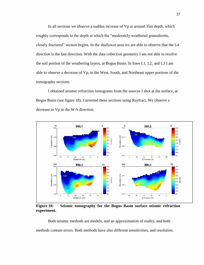
In all sections we observe a sudden increase of Vp at around 35m depth, which
roughly corresponds to the depth at which the “moderately weathered granodiorite,
closely fractured” section begins. In the shallower area we are able to observe that the L4
direction is the fast direction. With the data collection geometry I am not able to resolve
the soil portion of the weathering layers, at Bogus Basin. In lines L1, L2, and L3 I am
able to observe a decrease of Vp, in the West, South, and Northeast upper portions of the
tomography sections.
I obtained seismic refraction tomograms from the sources I shot at the surface, at
Bogus Basin (see figure 18). I inverted these sections using Rayfract. We observe a
decrease in Vp in the W-S direction.
Figure 18: Seismic tomography for the Bogus Basin surface seismic refraction
experiment.
Both seismic methods are models, and an approximation of reality, and both
methods contain errors. Both methods have also different sensitivities, and resolution.

38
The surface seismic has better power in resolving the near surface portion of the Bogus
Basin site. The reverse VSP dataset better resolves the overall velocity structure at depth.
The reverse VSP ray paths are closer to vertical and it may be harder to identify
azimuthal anisotropy, with such a data collection geometry.
2.2.3.2 Crossing point and fracture density
Figure 19 shows Vp values averaged at depth and fracture density for Bogus
Basin. In general, L3 appears to be the slowest direction, at most depths. At lower depths
L1, and L2 have the fastest velocities. In the shallowest section L4 displays the fastest
velocity.
From the fracture analysis done by Gates et al. (1994) at Bogus Basin, I assumed
that the direction of the main sets of fractures were in the N and E20°S directions. I used
Crampin et al. (1980) equations to solve for fracture density for each set of fractures. The
predominant set of fractures results to be north oriented. Both sets of fractures “close” at
around 45 m depth, using the reverse VSP dataset (figure 19).

39
Figure 19: Plot on the left represents the average Vp value at depth, for Bogus
Basin. Plot on the left is the fracture density at depth, for Bogus Basin. Blue line
represents fracture density for the N-S set of fractures, and the red line represents
fracture density for the N-S set of fractures, and the red line represents fracture
density for the E20°S set of fractures. (Note: the error bars represent the standard
deviation of Vp at depth).
2.2.3.3 Preferential orientation and percentage change
For Bogus Basin (figure 19) the slow Vp direction appears to be in the NE
direction. Again, I cannot resolve completely preferential fracture orientations, solely
based on my results, since I do not have enough azimuthal coverage.
In order to gauge fracture induced anisotropy, I calculated Vp percentage change
at Bogus Basin. If there’s large changes in Vp values I will be able to state, with more
confidence, the existence of fracture induced anisotropy.

40
I calculated velocity averages per line over depths of 20-50 m. I calculated
percentage change in Vp values from orientation to orientation, and are shown in table 4.
Yellow indicates the highest anisotropy values, and pink the lowest.
Table 4: Bogus Basin anisotropy values.
Vp
L2 L3 L4
L1 0.98 9.01 2.38
L2 9.90 3.33
L3 6.79
For Bogus Basin (table 4), we see little to no anisotropy between directions.
For the Bogus Basin site, to avoid inversion artifacts I decided to plot first arrival
travel times (figure 20), per azimuth. I only used picked travel times from 29-45 m depth,
due to the verticality of the well in that section (>0.5 m deviation from the top of the
borehole). I only used travel times from geophones 5 and 44 of each line, due to their
symmetry, and the completeness of picks in that particular section. Bogus Basin velocity
inversion shows no clear anisotropy, however plotting the travel times from 29-45 m
depth allows us to better observe anisotropy, within first arrival travel times.

41
Figure 20: Traveltimes (blue, cyan,red, and green), for the Bogus Basin reverse
VSP dataset (Note: 0° is N).
The preferential direction of fractures (see figure 22), should match the direction
of fast Vp (see figure 21). Three out of the 4 lines in which I surveyed at Bogus Basin,
match almost exactly the direction in literature (Gates et al., 1994) of possible fractures at
Bogus Basin; this was not actually intended. Seismic profiles were deployed in those
exact locations for logistic reasons (avoiding trees, or other structures).
I calculated a mean Vp, from the tomography sections, in 20 by 30 m regions,
from depths 20-50 m. The fast velocities correlate well with the direction of the
previously measured fracture sets. From mean Vp’s and mean fracture densities, I
modelled Vp at all azimuths, using Crampin et al. (1980) equations for two sets of
fractures.

42
Figure 21: Modelled Vp (blue, from eqns. 1-6), and the mean Vp, for each
direction (red), calculated for the depth range of 20-50 m, at Bogus Basin. (Note: 0°
is N).
Figure 22: Fracture orientations according to Gates et al. (1994), and geophone
locations at Bogus Basin.

43
2.3 Seismic refraction discussion
In hydrogeophysical studies, geophysical methods are used in the hopes of
obtaining a better understanding of hydraulic parameters such as fracture density,
porosity, hydraulic conductivity, etc (Knight and Endres, 2005). In order to obtain the
best possible hydrologic parameters, one has to begin with a good geophysical data
collection strategy to avoid obtaining misleading results in the hydrologic parameters. Of
course, even with a good geophysical data collection strategy, there are other possible
sources of error or uncertainty in the survey area (e.g. choosing an incorrect petrophysical
model, artifacts in the inversion of the geophysical parameters, etc.). However, planning
for a good survey is always the first step into obtaining a hydrologic model closer to the
true model. In my case, I surveyed in a known fractured area, therefore we expected
anisotropy in the geophysical parameters. From the seismic anisotropy measurements
(tables 2-4) I identify that the location that portrays the highest Vp azimuthal anisotropy
is Lower Weather.
In order to understand how much error might be introduced by assuming an
isotropic medium and collecting measurements in only one direction. I calculated
fracture density for each azimuth. I made the assumption that the medium contained
multiple sets of fractures in random orientations. This would be a valid assumption in
a mountain watershed underlain by fractured bedrock.
I used a model of randomly oriented vertical fractures to calculate fracture
density, described in detail in Berryman (2007):
𝜀 =−15
2
𝐺0
𝐸0𝜖
1 + 𝜈0
5 + 𝜈0 (10)

44
Where: 𝐺0, 𝐸0, and 𝜈0 are the background’s material shear modulus, Young’s
modulus, and Poisson’s ratio, respectively. 𝜖 is the Vp Thomsen anisotropy
parameter, and depends on the measured Vp and the Vp of the background material.
In order to derive equation 10 from Berryman (2007), I assumed a
noninteraction approximation from Berryman and Grechka (2006).
I used equation 10, to calculate fracture density using each survey’s Vp
values. I calculated the Lamé parameters using a Young modulus of 52, and a Poisson
ratio of 0.31, for the background material (obtained from Olona et al., 2010). I
assumed dry fractures and a background Vp of 3500 m/s. From the lithologic logs
near Lower Weather (figure 9) we see that the water table near Lower Weather is
roughly at around 50 m depth. I collected both seismic profiles at Lower Weather at
the end of summer, basically in the driest conditions. Therefore, assuming dry
fractures for this analysis is valid.
Figure 23 shows the fracture density calculated using equation 10, with the
ridge parallel survey (red), and the ridge perpendicular survey (blue). For comparison,
the minimized root mean square error (rmse) fracture density (eqn.8) using both
surveys appears in black.
Deciding to solely deploy a 2D survey, the obtained results would greatly vary
depending on the azimuth on which the survey was collected. From figure 23 we can
observe that the “parallel-random” line shows that most fractures close at around 27
m depth. The “perpendicular-random” line shows that most fractures close at around
53 m depth, and the minimized rmse line shows that most fractures close at around 28

45
m depth. Hydraulically, there is a big difference between having possibly active
hydraulic fractures closing at around 27 m, than at 52 m depth.
I must mention again that the “closure depth” is velocity dependent. I chose
3500 m/s for closure (from Olona et al., 2010). Such an assumption could be wrong.
Apparent fracture density values also change for every case, the rmse
minimized case has the widest range of values (from 0 to 1), both “parallel-random”
and “perpendicular-random” have a very linear behavior on the decrease of fracture
density with depth. For these reasons, when surveying in suspected fractured areas,
fracture induced hydraulic anisotropy must be taken into account to make good
hydrologic interpretations.

46
Figure 23: Fracture density calculated with a randomly oriented set of fractures
using the ridge-parallel survey (red), and the ridge-perpendicular survey (blue), both
at Lower Weather. The black line represents the minimized fracture density depth
profile obtained by using a model with one set of fractures and taking into account
the angle between suspected set of fractures and survey orientation.
Often times, CZ geophysicists deploy seismic surveys in order to obtain
measurements of depth to bedrock. If I decided to use only one of my profiles to calculate
depth to bedrock, I would get completely different results. I use a velocity contour of
3500 m/s (table 1) as a rough gauge of bedrock. Using the ridge parallel profile I would
obtain a depth to bedrock at 27 m depth. Using the ridge perpendicular profile I would
obtain a depth to bedrock at 53 m depth. Due to the anisotropy in the subsurface, we

47
obtain such a difference in our results. For fractured mountain watersheds, we should be
using 2D seismic profiles at different azimuths or even better, a full 3D seismic
deployment. These systems are too complex to be interpreted solely using one 2D profile
in one single orientation.
- My research hypothesis was: “there is a fracture system with a ridge parallel
preferential orientation, allowing deep weathering below the North Treeline ridge top”.
When analyzing the results from figures 10, 14, and 16 it appears that there is a striking
difference between Treeline ridges. In the NR, both sets of fractures appear to have an
effect in the Vp values we obtained. However, for the SR, the ridge perpendicular set of
fractures appears to have little to no effect on the Vp values. In the SR there is an obvious
slow velocity direction, and also a depth in which all directions sort of converge; this
depth is roughly the same depth at which fractures appear to close. In the NR, we can
infer there is a fast velocity direction, it is hard to determine a depth at which all or most
fractures converge.
Upon reviewing figure 15, we observe a clear slow and a fast direction. We
observe a fast, then a slow velocity at 0° and 45 ° respectively, from figure 15 NR
seismic plot. We observe the fastest direction at 90°, them a slow velocity at 135°, from
figure 15 NR seismic plot. These results match a model of two sets of orthogonal
fractures. However, we need more azimuthal coverage in order to validate the existence
of two sets of fractures.
A similar behavior is displayed in the SR. Changes in Vp values aren’t as
dramatic as in the NR. For both ridges, it is necessary to do a full 3D survey or collect
data at more azimuths if we want to better determine the orientation of all fracture sets.

48
- For control, I created histograms of fracture lineaments for the DCEW (figure 3)
and Treeline, based on the careful mapping study given by Acker (2008). From the
histograms (figure 24), I can determine roughly two main fracture orientations, in the
DCEW. One fracture orientation is in the NE direction (N 45° E), and the other
orientation appears to be in the SE direction (S 45° E). At Treeline, one dominant fracture
orientation is evident at around 150° from N. There are more fractures at other
orientations in Treeline, but they range azimuths from 0° to 45°, and 68° from the north.
From both histograms we observe that there’s a wide range in which fractures are present
in the DCEW, and Treeline. With my surveys, I was only able to measure Vp and ER at
four or two azimuths. I need better azimuthal coverage to be able to fully characterize the
fracture azimuthal variance.
Figure 24: Histograms of fracture lineament azimuth, for the DCEW and
Treeline.

49
- Locating a seismic source in the center of a circle of geophones is a method that
has been used in the past, for example, for shear wave propagation in anisotropic media
(Sondergeld and Rai, 1992). At different azimuths it is possible to see a change in shear
wave polarization, according to the material fabric.
For CZ purposes, other research groups (Steven Holbrook) have tackled the
characterization of fracture orientation by using the circle method for P-wave propagation
(Novitsky et al., 2016). Early arrival times correspond to the fracture orientation. This
method has a great advantage in the sense that the azimuthal coverage of geophones can
be high, without significantly increasing the physical labor in data collection. With a
denser azimuthal coverage it may be possible to resolve fracture orientation more
effectively in the case of multiple fracture sets. One of the down sides of this method is
that rough topography complicates the analysis, e.g. simple traveltime differences, as
interpreted by St. Clair et al. (2015) can be caused either by topography or by velocity
variation. Another problem is that we do not get much depth information with this
approach. We do not, at present, have a way to invert these data for velocity in the
presence of rough topography. Propagating a seismic wave into the saprolite or fractured
bedrock layer might be too hard for places with rough topography, in specific the absence
of long enough planar surfaces. Another element to look out for, while using this method,
is the existence of a possible dipping refractor below the surface, if there is, a correction
must be taken into account. The wagon-wheel method I used has the downside that the
azimuthal coverage is significantly lower, and increasing the azimuthal coverage implies
a significant increase in physical labor, by graduate students. A positive aspect of the
wagon-wheel method is that the 2D lines can extend for longer distances, as long as the

50
lines are maintained straight throughout the survey. This allows for deeper probing into
the subsurface. When topography is too rough and no geophones circles can be deployed,
the wagon-wheel array should be used. However, the best approach would be full 3D
seismic acquisition. There is currently software available for such inversions (e.g.
Geotomo). However, the field labor for collecting such data was beyond the resources
available for this project. It is still to be researched if the fracture orientation is preserved
from the fractured bedrock, all the way up to the saprolite. If this were to be the case, Vp
azimuthal variation due to fractures could be measured first with the circle method. To
characterize the deeper parts of the CZ, 2D seismic surveys could be deployed, at specific
azimuths.
2.4 Seismic refraction conclusions
My results suggest the presence of anisotropy at the surveyed sites. Lower
Weather displayed the highest anisotropy, up to almost 30%. We also determined
anisotropy at Treeline. Bogus Basin showed little to no anisotropy. Geophysical surveys
done at a mountain watershed underlain by fractured bedrock should take into account
the possibility of anisotropic medium. Therefore, data collection should be planned
accordingly. One single azimuth (e.g. a single 2D profile) is not sufficient to properly
characterize the fractured subsurface.
The “closure” of fractures is velocity dependent. The velocity I chose for fracture
closure is 3500 m/s, based on Olona et al. (2010). I admit this assumption could be
wrong. However, I am able to determine a major difference on calculating fracture
“closure” depth, using individual surveys at Lower Weather. Using solely the ridge
parallel profile we observe a depth of closure of around 27 m depth. On the other hand,

51
using the ridge perpendicular direction we observe depth of fracture closure of around 50
m depth. From this, we learn that several azimuths or better, a full 3D survey must be
collected in order to better characterize the “depth of fracture closure” in anisotropic
media.
One of our research objectives was to understand fracture orientation. However, I
recognize that to fully characterize fracture orientations we need more azimuthal
coverage.

52
CHAPTER THREE: ELECTRICAL RESISTIVITY TOMOGRAPHY
3.1 Electrical resistivity methods
3.1.1 Electrical resistivity tomography
An ordinary electrical resistivity survey consists in injecting electrical current into
the subsurface and measuring the electric potential. Any array of electrodes used to inject
current or measure potential can be set to study variations of electrical resistivity with
depth, lateral, and azimuthal variations in resistivity (Keller and Frischknecht, 1966). As
the spacing between electrodes increases, the depth probed also increases. The measured
electric potential depends on the material in which the survey is being conducted, because
different materials have different electrical resistivity values. Through the electric
potential measurements we are able to create a model of electrical resistivity of the
subsurface. The electrical resistivity model helps us better determine the presence of
structures or anomalies in the subsurface.
3.1.2 Electrical anisotropy
Electrical anisotropy is present when electrical resistivity varies depending on the direction
in which it is measured (Greenhalgh et al., 2010). Anisotropy can take place on a macro
scale when different isotropic layers behave as a single anisotropic system; fractures can
cause this effect. Resistivity values are usually larger (up to ten times) when measured
perpendicular to the direction of fractures (𝜌𝑡 known as transverse resistivity) in contrast
with the parallel values (𝜌𝑙 known as longitudinal resistivity, Yeboah-Forson and
Whitman, 2014).

53
Keller and Frischknecht (1966) defined two elements to characterize electrical anisotropy
in the subsurface, mean resistivity 𝜌𝑚 = √𝜌𝑡𝜌𝑙, and coefficient of anisotropy 𝜆 = √𝜌𝑡 𝜌𝑙⁄ .
When trying to detect electrical anisotropy using static ER measurements two strategies
are mainly used: ER lines deployed at varying azimuths (Taylor and Fleming, 1989; Zhu
et al., 2012; Busby, 2000), or square array techniques developed by Habberjam
(Habberjam and Watkins, 1967; Habberjam, 1971; Matias, 2002). Some studies have
resulted on measurements of electrical anisotropy coefficients (Yeboah-Forson and
Whitman, 2014; Busby, 2000; Zhu et al., 2012). It has been suggested that most cases of
anisotropy reported in the literature have been most likely misinterpretations
(Greenhalgh, 2008). Characterization of anisotropic media, using ER methods is a
research field that still needs advancements, in both the theoretical, and applied portions.
I can use a modified version of Archie’s law (Morey et al., 1984), to obtain a relation
between the measured DC conductivity (𝜎𝐷𝐶), porosity (𝜙), and water conductivity (𝜎𝑊):
𝜎𝐷𝐶 = 𝜎𝑊𝜙𝑟 (11)
Babcock et al. (2015) used the above relation for fully saturated sea ice cracks. I assume I
can use the same relation for fully saturated fractures, even though it hasn’t been
empirically verified. I use the same values as Morey et al. (1984) for the r exponent, with
𝑟 = 1.75 if the profile is fracture parallel or 𝑟 = 1.55 if the profile is fracture
perpendicular.
3.1.3 Electrical resistivity data collection
I collected all ERT profiles using the Syscal Pro instrument, by IRIS instruments.
The setup for all of my ERT data collection was: 72 channels, using both Wenner and
dipole-dipole arrays, with an electrode spacing of 5 m.

54
For both the ERT profiles at Lower Weather, I deployed two orthogonal profiles,
one ridge parallel and one ridge perpendicular (figure 25). Both ER profiles were
collected at the end of Spring 2017.
Figure 25: Map of ERT data collection at the Lower Weather site.
For the Treeline ERT data collection I collected data at three different azimuths,
at each ridge (see figure 26). The profile crossing both ridges (L1) was collected in the
Fall 2014, by the electrical and electromagnetic methods class of 2014, of the Department
of Geosciences, at Boise State University. The remaining four profiles were collected in
the Fall of 2016.

55
Figure 26: Map of ER data collection at Treeline.
3.1.4 Electrical resistivity data processing
I used the commercial software RES2DInv to invert the data. The inversion
method I used was a finite difference, smoothed least-squares scheme, I included the
errors in the measurement to improve the inversion results. I removed bad data points
with standard deviations above 35%. According to Loke et al. (2003), one of the most
commonly used methods to invert ERT data is the least-squared optimization method,
with a smoothness-constraint or L2 norm. This method minimizes the sum of squares of
the spatial changes in the model resistivity and the data misfit. It yields better results
when the changes in the subsurface are smooth (Barker, 1996). Although, when clear,
sharp boundaries exist, this method tends to smear them out.

56
3.2 Electrical resistivity results
3.2.1 Lower Weather results
3.2.1.1 Tomograms
Figure 27 shows the 2D ERT inversion results for Lower Weather. We observe
ER heterogeneity in both directions, ridge parallel and ridge perpendicular. The sections
are both laterally and vertically heterogeneous, making it difficult to interpret in terms of
a simple weathering model.
Figure 27: Electrical resistivity tomography for the Lower weather site. Black
lines represent the crossing point between both surveys. Contoured sections display a
higher ER, distinctive of fresh granite (see table 1).
I additionally present ER pseudo-sections for Lower Weather in the Appendix
(figure 35).
Electrical characterization of fractured systems is by itself a complicated task, if
the system includes clays, this task becomes more challenging. We see from the
lithologic logs (figure 9) that clays are found at the very top of the depth profile, near

57
Lower Weather. We also see clays at depth in one of the wells near Lower Weather.
Clays have low ER when wet and high ER when dry. The inversion models I used are
highly regularized, in order to get a stable solution. These high regularizations might
interfere in the correct resolution of fractures in the subsurface, and yield smoothed
models. I believe my Lower Weather ERT profiles are hard to interpret, because we have
an especially complex system in the subsurface.
3.2.1.2 Crossing points
To compare data collected at different azimuths, I took a 20 m section centered at
the crossing point, for every azimuth, then I calculated an average resistivity as a function
of depth. Figure 28 represents the averaged section, at the crossing point in Lower
Weather. Due to the presence of many heterogeneities in the ERT profiles, interpreting
such results for electrical anisotropy purposes is impossible.

58
Figure 28: Average ER at depth with error bars, at Lower Weather. The blue line
represents the parallel direction, and the red line represents the perpendicular
direction. (Note: the error bars represent the standard deviation of ER at depth).
Based solely on the ER results I am unable to prove ER anisotropy at Lower
Weather. The uncertainty and heterogeneity is too high to make any firm conclusions.
3.2.1.3 Preferential orientation
The preferential direction for fractures, should match the direction of low ER. I
plotted a mean ER per azimuth, in figure 29 (shown in red). I calculated the mean ER
from 5-25 m depth, from figure 28. I fitted an ellipse to the mean ER values. We observe
from figures 11 and 29 that the direction of low ER matches the direction of the fast Vp.

59
This observation agrees, qualitatively, with what is expected for ER values. However, I
must recognize that our ER results for Lower Weather are too heterogeneous and too
uncertain to make firm conclusions on anisotropy matters.
Figure 29: Best fitted ellipse (blue) and the mean ER, for each direction (red).
(Note: 0° is N).
3.2.2 Treeline results
3.2.1.1 Tomograms
Figure 30 shows the 2D inversion results for the Treeline ERT surveys. We
observe more ER heterogeneity in the NR than in the SR. Interpretation of 2D ERT
results, for weathering purposes, is difficult solely using this method. Major high ER
resistivity anomalies are observed, mainly in the NR such anomalies are also present in
the seismic results (see figures 12-13). The utilization of 2D ERT for granite weathering
states is best when complemented with another geophysical method.

60
Figure 30: Electrical resistivity tomography for Treeline. Black lines represent the crossing point between both
surveys (bold lines are the main crossing points, and the dotted lines represent other crossing points). Contoured sections
display a higher resistivity, representative of fresh granite (see table 1).
I additionally present ER pseudo-sections for Treeline in the Appendix (figure 37).

61
3.2.1.2 Crossing points
Figure 31 represents the averaged sections at depth for the main Treeline
crossings. There isn’t a clear anisotropic behavior of ER as a function of depth. The ridge
parallel has the highest ER, and the ridge perpendicular has the lowest ER, in both ridges,
as shown in the plots below. At lower depths this behavior changes that is why I can’t
affirm with high certainty the existence of ER anisotropy at Treeline based on these
results only. ER is generally higher and more homogeneous in the SR. This is consistent
with less fracturing in the SR than in the NR.
Figure 31: Average ER at depth with error bars, at the Treeline site. The blue line
represents the parallel direction, the red line represents the perpendicular direction,
and the green line represents the E-W direction. (Note: the error bars represent the
standard deviation of ER at depth).
Based solely on the ER results I am unable to prove ER anisotropy at Treeline.
The uncertainty is too high to make any firm conclusions.

62
3.2.1.3 Preferential orientation
The preferential direction of fractures should match the direction of low ER.
I plotted a mean ER per azimuth, in figure 32 (in red). I calculated the mean ER
from 5-25 m depth of figure 31. I fitted an ellipse (in blue) from the mean ER values, for
all azimuths.
The fitted ER ellipses for the NR and SR are roughly tilted in the same direction;
meaning, both have the smallest ER in the NE-SW direction.
The minor axis of the fitted ellipse should roughly point to the direction of the
dominant set of fractures. For the SR, the direction of the ER minor axis point to the NE-
SW direction, which roughly coincides with the direction of the fast Vp direction (figures
15 and 32). However, I cannot confirm with certainty a preferential fracture orientation
with the small range of azimuthal coverage in the survey.
Figure 32: Best fitted ellipses (blue) and mean ER, for each direction (red). (Note:
0° is N).

63
3.3 Electrical resistivity discussion
I wasn’t able to resolve preferential fracture orientation with ER measurements. I
also wasn’t able to determine the different weathered layers of the CZ, at any of the sites
I collected data. Roubinet and Irving (2014) suggest that the current numerical modeling
tools are not well suited for the complexity of fractured media. Current numerical
methods consider heterogeneities to be of a particular grid size. Fractures vary in size and
aperture, and within a given volume in the subsurface. Current methods “blur-out” these
fracture caused heterogeneities, so we are not able to resolve them. However, efforts are
being done currently to improve the modeling of electrical conduction through fractured
media (Roubinet et al., 2016; Caballero-Sanz et al., 2017).
3.4 Electrical resistivity conclusions
My ER results are too uncertain and heterogeneous to make clear statements on
electrical anisotropy. Solely using 2D ERT methods to characterize fractured media is not
suggested. At least not with the current inversion methodology available. These fractured
systems are too complex to be fully characterized using a 2D approach. However, new
methodologies or 3D surveys could help us better resolve fractures.

64
CHAPTER FOUR: WEATHERING DEPTH
4.1 Weathering depth results
4.1.1 Weathering depth as a function of elevation
I used the seismic refraction results to calculate depth to bedrock at all sites. I
used a 3500 m/s contour (table 1) as a rough gauge to calculate depth to bedrock in all 2D
surface seismic refraction profiles (tables 5-6). Using a single velocity value to calculate
weathering depth in an anisotropic system is incorrect. It is important to mention that
these measurements are the mean and lateral variability along a single seismic profile.
Correct characterization would require full 3D data, anisotropic inversion, and an
anisotropic petrophysical model. I use this single velocity value more as a qualitative
measure to get a rough estimate of relative variation as a function of site elevation and
aspect.
At Lower Weather, in the ridge parallel profile (figure 8) I measured a depth to
bedrock of 30 ± 10 m. For the ridge perpendicular profile, I measured a depth to bedrock
of 28 ± 16 m. The mean depth to bedrock at Lower weather is 29 ± 16 m.
Table 5: Mean depth to bedrock at the Treeline site.
TREELINE
PROFILE Mean Depth to bedrock (m) Standard deviation (m)
L1 29 14
L2 28 8
L3 20 11

65
L4 24 10
L5 20 12
L6 16 9
L7 21 10
Overall the average depth to bedrock at Treeline is 23 ± 12 m. From table 5, we
see that overall the seismic profiles collected in the SR (L5, L6, and L7) show a
shallower bedrock. This agrees with less fracturing in the SR than in the NR.
Overall the average depth to bedrock at Bogus Basin is 5 ± 2 m (see table 6). I
decided to calculate the depth to bedrock using the surface seismic at Bogus Basin,
instead of the reverse VSP data, to be consistent within the seismic method used to
calculate depth to bedrock in the rest of the locations.
Table 6: Mean depth to bedrock at the Bogus Basin site.
BOGUS BASIN
PROFILE Mean Depth to bedrock (m) Standard deviation (m)
BBL1 4 1
BBL2 5 1
BBL3 6 3
BBL4 6 1
4.1.2 Weathering depth per aspect per site
I calculated the weathering layer thicknesses as a function of aspect at Lower
Weather (Table 7). I assumed mobile soil to be within the 0-700 m/s Vp values, saprolite
to be within 700-2000 m/s, and fractured granite to be within 2000-3500 m/s, according
to Olona et al. (2010, see table 1). I am aware that the results given below (tables 7-9) are

66
mere approximations, because these data are taken from an inverse model; therefore these
are subject to smoothing of boundaries due to regularizations.
In Lower Weather, due to the relatively course 5 m geophone spacing, I was
unable to resolve the mobile soil layer.
Table 7: Weathering layer thicknesses for the Lower weather site. (Note: the ±
indicates standard deviation per aspect, not error).
Layer Aspect Thickness (m) Average (m)
0-700 m/s
(Mobile soil?)
W 0
0 N 0
S 0
700-2000 m/s
(Saprolite?)
W 5.99 ± 2.49
8.12 N 9.91 ± 5.42
S 8.47 ± 2.96
2000-3500 m/s
(Fractured granite?)
W 32.99 ± 5.58
24.5 N 15.19 ± 12.34
S 25.33 ± 9.23
At Lower Weather, the West aspect has the least thick saprolite layer (5.99 ± 2.49
m), but the thickest fractured granite layer (32.99 ± 5.58 m). On the contrary, the North
aspect has the thickest saprolite layer (9.91 ± 5.42 m), but the least thick fractured
bedrock layer (15.19 ± 12.34 m).

67
Table 8: Weathering layer thicknesses for the NR at Treeline. (Note: the ±
indicates standard deviation per aspect, not error).
Layer Aspect Thickness (m) Average (m)
0-700 m/s
(Mobile soil?)
E 0.05 ± 0.22
0.10 SW 0.24 ± 0.57
SE 0
S 0
700-2000 m/s
(Saprolite?)
E 5.64 ± 2.79
7.06 SW 6.02 ± 3.67
SE 8.13 ± 2.67
S 8.43 ± 2.61
2000-3500 m/s
(Fractured granite?)
E 19.85 ± 12.60
20.12 SW 29.11 ± 7.95
SE 16.70 ± 7.05
S 14.83 ± 10.11

68
Table 9: Weathering layer thicknesses for the SR at Treeline. (Note: the ±
indicates standard deviation per aspect, not error).
Layer Aspect Thickness (m) Average (m)
0-700 m/s
(Mobile soil?)
E 0.02 ± 0.13
0.06 NW 0.16 ± 0.45
W 0
700-2000 m/s
(Saprolite?)
E 5.85 ± 3.50
6.33 NW 11.57 ± 5.97
W 1.57 ± 1.97
2000-3500 m/s
(Fractured granite?)
E 11.45 ± 6.20
11.08 NW 12.28 ± 8.80
W 9.50 ± 6.30
In Treeline’s NR, the aspects with the thinnest saprolite layers are the East (5.64 ±
2.79 m) and Southwest (6.02 ± 3.67 m) aspects; these correspond to the thickest fractured
bedrock layers (29.11 ± 7.95 m for the Southwest aspect and 19.85 ± 12.60 m for the East
aspect).
The thickest saprolite layers are present in the Southeast (8.13 ± 2.67 m) and
South (8.43 ± 2.61 m) aspects. However, these aspects correspond to the least thick
fractured bedrock layers (16.70 ± 7.05 m for the Southeast aspect and 14.83 ± 10.11 m
for the South aspect).
Treeline’s SR is the only location where this change in least thick, to thickest
layers (and vice versa) doesn’t happen. For the SR, the thinnest saprolite layer is located
in the West aspect, and the thickest is located in the Northwest aspect; the same trend
continues for the fractured bedrock layer.

69
4.2 Weathering depth discussion
- Seismic profiles 4, 5, and 7 (figure 33) end in a Northwest facing aspect,
where vegetation changes from grass and shrubs to a tree dominated area. The
thickness of the saprolite layer in the NW aspect at the SR in Treeline is 11.57 ± 5.97
m, the highest calculated at either Lower Weather or Treeline, and more than twice as
thick as observed on any other aspect at Treeline.
Figure 33: Zoom into forested area at Treeline.
If I was only to compare the different aspects in the SR at Treeline, I would
preserve: local and regional stress, and roughly the same level of the water table. The
elements that change among aspects are: aspect itself, vegetation type, solar input,
and snow accumulation.
L4
L5
L7

70
I hypothesize there is a positive interaction of various elements that favors
weathering at this specific site. There is likely more vegetation because of water
availability and solar input. The increased vegetation in turn holds more moisture and
the roots enhance weathering.
Kormos et al. (2014) suggests that at Treeline snow remains for longer
periods of time in North facing aspects. Anderson et al. (2014) showed that forested
areas hold snow for longer periods of time within the DCEW. Langston et al. (2015)
present models indicating that a large sustained recharge pulse forces more water
deeper into the saprolite matrix and the fractures than repeated, smaller recharge
events. Therefore if there’s more snow throughout the winter at the NW facing slope
at Treeline, due to the vegetation and aspect, there’s more weathering happening
because of the possible duration of snow cover in that area. More snow research
needs to be done at this specific aspect in Treeline to prove this hypothesis.
The NW aspect at Treeline has a higher tree density, than the rest of Treeline.
I believe the tree roots permit meteoric fluids to penetrate deeper into the subsurface
promoting weathering processes. Some studies suggest that there is a positive
feedback between increase in tree density and increase in weathering (Gabet and
Mudd, 2010; Ebel et al., 2015). More research needs to be done to determine exactly
the main factors increasing weathering in Treeline, overall. More focused seismic
profiles can be carried out in the NW aspect at Treeline.
- The model of St. Clair et al. (2015) explains that both topography and regional stress
play a role in bedrock fracture distribution (Moon et al., 2017). In some cases, a
“bow-tie” effect happens under ridges, meaning, there is an increase in fractures

71
below ridge tops, therefore there is a decrease in Vp below ridge tops, this effect has
been referred as “the bow-tie effect” or “mirroring effect”. This can also be seen as
the depth to bedrock not always following the topography, but rather it sometimes
mirrors the topography.
Not all seismic profiles collected in this research allow to observe distinctly
the “bow-tie effect”, because I didn’t capture both ridge top and ridge bottom in all
my profiles. Although, we can distinctly observe the “bow-tie effect” in lines 1, 3, 4,
and 6, from figures 12 and 13, and the ridge perpendicular profile in figure 8. A
detailed analysis of local stress at the DCEW is needed to better understand the
spatial distribution of the least compressive stress. Having a detailed analysis on
stress at the DCEW will help us better predict zones of high fracturing.
- In my study I found that the average thickest saprolite, and fractured bedrock layers,
are present at the lowest elevation (Lower Weather) site, and the thinnest saprolite is
at the Bogus Basin site (figure 34). The elevation difference between Treeline and
Lower Weather is approximately 500 m. The elevation difference between Bogus
Basin and Lower Weather is approximately 800 m.

72
Figure 34: Depth to bedrock and saprolite thickness as a function of elevation.
The overall depth of the weathering zone decreases with increasing elevation.
The mean depth to bedrock at Lower weather is 29 m, at Treeline 23 m, and at Bogus
Basin 5 m.
An increase in weathering with decreasing elevations has also been observed
at Johnston’s Draw, Reynolds Creek Critical Zone Observatory, by Nielson (2017).
As noted by Nielson, this trend is likely caused by the increasing temperature with
decreasing elevations, and this is consistent with other studies (Rasmussen et al.,
2010; Rech et al., 2001).

73
4.3 Weathering depth conclusions
The calculation of depth to bedrock is velocity dependent. I assumed the granitic
bedrock at my sites has a Vp of 3500 m/s (from Olona et al., 2010). I recognize this
model could be wrong, however this single value does provide a basis for interpretation
of relative variations.
From the surface seismic refraction data collections I observe that depth to
bedrock increases with decreasing elevation. This same pattern has been observed in the
Reynolds Creek Critical Zone Observatory. It has been hypothesized that this feature
could be related with increasing temperatures at lower elevations. Higher temperatures
could increase reactivity in weathering processes.
Comparing the use of seismic refraction vs. ERT to delineate weathered layers, I
conclude that seismic refraction is a more suitable method than ERT.
I observed a significant increase in weathering at a Northwest facing slope in
Treeline. This slope has higher tree density than the rest of Treeline. Therefore, I believe
that there is a positive feedback between tree roots and fractures as well as moisture
delivery and solar input that promotes weathering in this specific site. Since this is a
northern aspect, it most likely retains moisture better than southern aspects. This
additional effect could also promote weathering at this site.

74
CHAPTER FIVE: CONCLUSIONS AND RECOMMENDATIONS
I conducted a series of 2D ERT and seismic refraction surveys in the DCEW, at
three different elevations: Lower Weather, Treeline, and Bogus Basin. At each site, I
collected the surveys at different azimuths, with a common crossing point. I was able to
determine, slow or fast velocity directions at each site, but I am not able to fully
characterize the preferential fracture orientation, at any site; to do so, I need more
azimuthal coverage in my experiment. I suggest to carry out full 3D seismic surveys to
improve my azimuthal resolution power.
In Treeline’s NR, fractures seem to mostly close at around 25 m depth. At the SR,
fractures mostly close at around 15 m depth. Fractures appear to close at around 27 m
depth, in Lower Weather. Depth to unweathered bedrock is highest at Lower Weather. It
is important to mention, that due to the scales I’m working in my seismic refraction
surveys, with seismic waves spanning up to tens of meters in wavelengths, I am able to
resolve that most fractures are closed at the aforementioned depths. I am not able to
resolve the effect of a single or very few fractures on Vp. At “closure depth” I mean
fracture density is significantly lower. The fracture density “closure” depends on
velocity. I assumed the fractures would close at 3500 m/s. However, I am aware this
assumption could be wrong. My results show that anisotropy continues deeper than my
closure depth, this indicates that fractures are still present at lower depths; I’m just not
able to fully resolve them. A better rocks physics model, for the granite at the DCEW
could help me improve this aspect.

75
From the seismic surveys done at Treeline (figures 12and 13) I am able to identify
an area of high weathering at Treeline, in a NW facing slope. The main difference
between this specific area and the rest of Treeline is the type of vegetation, and aspect.
Therefore I believe there is a positive feedback between vegetation type, soil moisture,
solar flux, and weathering, at Treeline.
Geophysical surveys can be carried out to help characterize subsurface hydrologic
parameters. When surveying in a fractured area, one has to take into account the
possibility of fracture induced anisotropy. Neglecting fracture induced anisotropy can
lead to erroneous interpretations of the subsurface hydrologic system.
My results suggest the presence of anisotropy at the surveyed sites. Lower
Weather displayed the highest anisotropy, up to almost 30%. I also determined anisotropy
at Treeline. Bogus Basin showed little to no anisotropy. Geophysical surveys done at a
mountain watershed underlain by fractured bedrock should take into account the
possibility of anisotropic medium. Therefore, data collection should be planned
accordingly. One single azimuth (e.g. a single 2D profile) is not sufficient to properly
characterize the fractured subsurface.
There are more geophysical tools that can be used in the future to better
characterize the hydrologic system at the DCEW. S-wave velocity is more sensitive to
fractured media and is subject to birefringence (different polarizations traveling as
different modes in the same direction with differing velocity), therefore, it could be a
powerful tool to characterize the fractured system at the DCEW. I recognize that S-wave
data collection is logistically more complicated than P-wave data collection. S-wave data
collection was beyond the scope of this investigation.

76
In the hope of upscaling the overall effect of fractures at the DCEW, a seismic
interferometry survey could be carried out to characterize in a bigger scale the subsurface
of the DCEW.
In order for seismic interferometry to work, we need a source of seismic noise.
The road from Boise to Bogus Basin is regularly transited by vehicles. Vehicles could be
a useful source of seismic noise in low frequencies. Low frequency waves are able to
travel deeper into the subsurface allowing us to probe the subsurface at the watershed
scale.
To do a better job in a petrophysical analysis, we need a deep knowledge of the
mineralogy of the subsurface, collecting deep borehole geologic data would be especially
useful. A detailed research of the stresses in the DCEW is also suggested to better predict
areas of bedrock weathering.

77
REFERENCES
Acker, B. (2008). Scale and heterogeneity in hydraulic properties of the fractured
bedrock granitic Boise front, Boise, Idaho. (Unpublished Master’s thesis).
Retrieved from: Boise State University Library (Thesis GB1025.I2 H64 2008).
Aishlin, P., & J.P. Mcnamara (2011). Bedrock infiltration and mountain block recharge
accounting using chloride mass balance. Hydrological Processes.
http://doi.org/10.1002/hyp.7950
Aldridge, D. F., & D.W. Oldenburg (1993). Two-dimensional tomographic inversion
with finite-difference traveltimes. Journal of Seismic Exploration, 2, 257–274.
Anderson, B. T., Mcnamara, J. P., Marshall, H. P., & A.N. Flores (2014). Insights into
the physical processes controlling correlations between snow distribution and
terrain properties. Water Resources Research, 50, 1–19.
http://doi.org/10.1002/2013WR013714
Anderson, R. S., Anderson, S. P., & G.E. Tucker (2013). Rock damage and regolith
transport by frost : an example of climate modulation of the geomorphology of the
critical zone. Earth Surface Processes and Landforms, 38, 299–316.
http://doi.org/10.1002/esp.3330
Anderson, S. P., Von Blanckenburg, F., & A.F. White (2007). Physical and Chemical
Controls on the Critical Zone. Elements, 3, 315–320.
Babcock, E. L., Bradford, J. H., & C. Hall (2015). Cold Regions Science and Technology
Electrical anisotropy in sea ice and a dual-polarization radar system to mitigate
the effects of preferential attenuation in imaging sea ice. Cold Regions Science
and Technology, 118, 105–111. http://doi.org/10.1016/j.coldregions.2015.06.012

78
Barker, R.D. (1996). The application of electrical tomography in groundwater
contamination studies: EAGE 58th Conference and Technical Exhibition
Extended Abstracts, 744-747.
Befus, K. M., Sheehan, a. F., Leopold, M., Anderson, S. P., & R.S. Anderson (2011).
Seismic Constraints on Critical Zone Architecture, Boulder Creek Watershed,
Front Range, Colorado. Vadose Zone Journal, 10(4), 1342.
http://doi.org/10.2136/vzj2010.0108er
Berryman, J. G., & G.M. Hoversten (2013). Modelling electrical conductivity for earth
media with macroscopic fluid-filled fractures. Geophysical Prospecting, 61, 471–
493. http://doi.org/10.1111/j.1365-2478.2012.01135.x
Berryman, J. G. (2007). Seismic waves in rocks with fluids and fractures. Geophysical
Journal International, 171, 954–974. http://doi.org/10.1111/j.1365-
246X.2007.03563.x
Berryman, J. G., & Grechka, V. (2006). Random polycrystals of grains containing
cracks : Model of quasistatic elastic behavior for fractured systems Random
polycrystals of grains containing cracks : Model of quasistatic elastic behavior for
fractured systems. Journal of Applied Physics, 100(113527).
http://doi.org/10.1063/1.2399891
Burns, D.R., Willis, M.E., & M.N. Toksoz (2007). Fracture properties from seismic
scattering. The Leading Edge.
Busby, J. P. (2000). The effectiveness of azimuthal apparent-resistivity measurements as
a method for determining fracture strike orientations. Geophysical Prospecting,
48, 677–696.
Caballero-Sanz, V., Roubinet, D., Demirel, S., & Irving, J. (2017). 2.5-D discrete-dual-
porosity model for simulating geoelectrical experiments in fractured rock.
Geophysical Journal International, 209, 1099–1110.
http://doi.org/10.1093/gji/ggx080
Crampin, S., Mcgonigle, R., & D. Barnford (1980). Estimating crack parameters from
observations of P-wave velocity anisotropy. Geophysics, 45(3).

79
Crampin, S. (1985). Evaluation of anisotropy by shear-wave splitting. Geophysics, 50(1),
142–152.
Ebel, B. A., Rengers, F. K., & G.E. Tucker (2015). Aspect-dependent soil saturation and
insight into debris-flow initiation during extreme rainfall in the Colorado Front
Range. Geology, 43(8), 659–662. http://doi.org/10.1130/G36741.1
Gabet, E. J., & S.M. Mudd (2010). Bedrock erosion by root fracture and tree throw : A
coupled biogeomorphic model to explore the humped soil production function and
the persistence of hillslope soils. Journal of Geophysical Research, 115.
http://doi.org/10.1029/2009JF001526
Gates, W. C. B., Parkinson, C. L., & K.L. Schroeder (1994). Groundwater development
in granitic terrain Bogus Basin ski resort. In Hydrogeology, Waste disposal,
Science and politics proceedings.
Greenhalgh, M.S. (2008). DC Resistivity modelling and sensitivity analysis in anisotropic
media. (PhD thesis) Retrieved from the University of Adelaide Library.
Greenhalgh, S. A. G., Marescot, L. M., Zhou, B. Z., Greenhalgh, M. G., & T.W. Wiese
(2009). Electric Potential and Frechet Derivatives for a Uniform Anisotropic
Medium with a Tilted Axis of Symmetry. Pure and Applied Geophysics, 166,
673–699. http://doi.org/10.1007/s00024-009-0465-6
Greenhalgh, S., Wiese, T., & L. Marescot (2010). Comparison of DC sensitivity patterns
for anisotropic and isotropic media. Journal of Applied Geophysics, 70(2), 103–
112. http://doi.org/10.1016/j.jappgeo.2009.10.003
Habberjam, G.M., and G.E. Watkins (1967). The use of a square configuration in
resistivity prospecting. Twenty-ninth meeting of the European Association of
Exploration Geophysicists.
Habberjam, G.M. (1971). The effects of anisotropy on square array resistivity
measurements. Thirty-third meeting of the European Association of Exploration
Geophysicists.
Holbrook, W. S., Riebe, C. S., Elwaseif, M., Hayes, J. L., Basler-Reeder, K., Harry, D.
L., Armen, M., Dosseto, A., Hartsough, P.C., & J.W. Hopmans (2014).
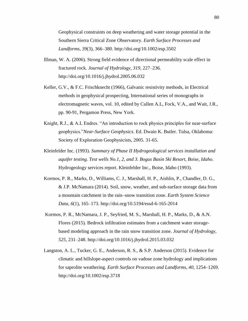
80
Geophysical constraints on deep weathering and water storage potential in the
Southern Sierra Critical Zone Observatory. Earth Surface Processes and
Landforms, 39(3), 366–380. http://doi.org/10.1002/esp.3502
Illman, W. A. (2006). Strong field evidence of directional permeability scale effect in
fractured rock. Journal of Hydrology, 319, 227–236.
http://doi.org/10.1016/j.jhydrol.2005.06.032
Keller, G.V., & F.C. Frischknecht (1966), Galvanic resistivity methods, in Electrical
methods in geophysical prospecting, International series of monographs in
electromagnetic waves, vol. 10, edited by Cullen A.L, Fock, V.A., and Wait, J.R.,
pp. 90-91, Pergamon Press, New York.
Knight, R.J., & A.L Endres. “An introduction to rock physics principles for near-surface
geophysics.”Near-Surface Geophysics. Ed. Dwain K. Butler. Tulsa, Oklahoma:
Society of Exploration Geophysicists, 2005. 31-65.
Kleinfelder Inc. (1993). Summary of Phase II Hydrogeological services installation and
aquifer testing. Test wells No.1, 2, and 3. Bogus Basin Ski Resort, Boise, Idaho.
Hydrogeology services report. Kleinfelder Inc., Boise, Idaho (1993).
Kormos, P. R., Marks, D., Williams, C. J., Marshall, H. P., Aishlin, P., Chandler, D. G.,
& J.P. McNamara (2014). Soil, snow, weather, and sub-surface storage data from
a mountain catchment in the rain–snow transition zone. Earth System Science
Data, 6(1), 165–173. http://doi.org/10.5194/essd-6-165-2014
Kormos, P. R., McNamara, J. P., Seyfried, M. S., Marshall, H. P., Marks, D., & A.N.
Flores (2015). Bedrock infiltration estimates from a catchment water storage-
based modeling approach in the rain snow transition zone. Journal of Hydrology,
525, 231–248. http://doi.org/10.1016/j.jhydrol.2015.03.032
Langston, A. L., Tucker, G. E., Anderson, R. S., & S.P. Anderson (2015). Evidence for
climatic and hillslope-aspect controls on vadose zone hydrology and implications
for saprolite weathering. Earth Surface Processes and Landforms, 40, 1254–1269.
http://doi.org/10.1002/esp.3718

81
Li, P., & F. Uren (1997). Analytical Solution for the Point Source Potential in an
Anisotropic 3-D Half-Space I: Two-Horizontal-Layer Case. Mathematical and
Computer Modelling, 26(5), 9-27. https://doi.org/10.1016/S0895-7177(97)00155-
6
Lynn, H., & R.J. Michelena (2011). Practical applications of anisotropy. The Leading
Edge, 30(7), 726-730.
Loke, M. H., Acworth, I., & T. Dahlin (2003). A comparison of smooth and blocky
inversion methods in 2D electrical imaging surveys. Exploration Geophysics,
34(3), 182–187.
Miller, C. R., Routh, P. S., Brosten, T. R., & J.P. McNamara (2008). Application of time-
lapse ERT imaging to watershed characterization. Geophysics, 73(3), 7–17.
http://doi.org/10.1190/1.2907156
Matias, M. J. S. (2002). Square array anisotropy measurements and resistivity sounding
interpretation. Journal of Applied Geophysics, 49(3), 185–194.
http://doi.org/10.1016/S0926-9851(01)00113-6
Moon, S., Perron, J. T., Martel, S. J., Holbrook, W. S., & J. St. Clair (2017). A model of
three-dimensional topographic stresses with implications for bedrock fractures,
surface processes, and landscape evolution. Journal of Geophysical Research, 1–
24. http://doi.org/10.1002/2016JF004155
Morey, R.M., Kovacs, A., & G.F.N Cox (1984). Electromagnetic properties of sea ice.
Cold Reg.Sci. Technol. 9 (1), 53–75.
National Research Council (2001), Basic research opportunities in earth science, National
Academy Press, Washington, DC.
Nielson, T. (2017). Application of hydrogeophysical imaging in the Reynolds Creek
Critical Zone Observatory. (Unpublished Master’s thesis). Retrieved from: Boise
State University Library
Novitsky, C.G., Holbrook, W.S., Carr, B., & S. Pasquet (2016), Fracture orientation in
the shallow critical zone from seismic anisotropy, Abstract EP43C-0969
presented at 2016 Fall Meeting, AGU, San Francisco, Calif., 11-15 Dec.

82
Olona, J., Pulgar, J. A., Fernández-Viejo, G., López-Fernández, C., & J.M. González-
Cortina (2010). Weathering variations in a granitic massif and related
geotechnical properties through seismic and electrical resistivity methods. Near
Surface Geophysics, 8, 585–599. http://doi.org/10.3997/1873-0604.2010043
Parham, W.B. (2015). Spatial and temporal storage dynamics moderate the ecohydrologic
significance of evapotranspiration in semi-arid mountainous terrain. (Unpublished
Master’s thesis). Retrieved from: Boise State University Library
Poulos, M.J. (2016) "Feedbacks among climate, soils, vegetation, and erosion drive
valley asymmetry development in the mountains of central Idaho". Boise State
University Theses and Dissertations.
Rasmussen, C., Dahlgren, R. A., & R.J. Southard (2010). Basalt weathering and
pedogenesis across an environmental gradient in the southern Cascade Range,
California, USA. Geoderma, 154(3-4), 473–485.
http://doi.org/10.1016/j.geoderma.2009.05.019
Rech, J. A., Reeves, R. W., & D.M. Hendricks (2001). The influence of slope aspect on
soil weathering processes in the Springerville volcanic field, Arizona. Catena, 43,
49–62.
Rempe, D. M., & W.E. Dietrich (2014). A bottom-up control on fresh-bedrock
topography under landscapes. Proceedings of the National Academy of Sciences
of the United States of America, 111(18). http://doi.org/10.1073/pnas.1404763111
Riebe, C. S., Hahm, W. J., & S.L. Brantley (2016). Controls on deep critical zone
architecture : a historical review and four testable hypotheses. Earth Surface
Processes and Landforms. http://doi.org/10.1002/esp.4052
Roubinet, D., & Irving, J. (2014). Journal of Geophysical Research : Solid Earth
Discrete-dual-porosity model for electric current flow in fractured rock. Journal
of Geophysical Research: Solid Earth, 119, 767–786.
http://doi.org/10.1002/2013JB010668.Abstract
Roubinet, D., Linde, N., Jougnot, D., & Irving, J. (2016). Streaming potential modeling
in fractured rock : Insights into the identification of hydraulically active fractures.

83
Geophysical Research Letters, 4937–4944.
http://doi.org/10.1002/2016GL068669.Numerous
Schuster, G. T., & A. Quintus-bosz (1993). Wavepath eikonal traveltime inversion:
Theory. Geophysics, 58(9), 1314–1323.
Sondergeld, C. H., & Rai, C. S. (1992). Laboratory observations of shear-wave
propagation in anisotropic media. The Leading Edge, 11(2), 38–43.
St. Clair, J., Moon, S., Holbrook, W. S., Perron, J. T., Riebe, C. S., Martel, S. J., Carr, B.,
Singha, K., & D. de B. Richter (2015). Geophysical imaging reveals topographic
stress control of bedrock weathering. Science, 350(6260), 534–539.
Taylor, R. W., & A.H. Fleming (1989). Characterizing Jointed systems by Azimuthal
Resistivity Surveys. Groundwater, 26(4).
Tsvankin, I., and V. Grechka (2011), Seismology of Azimuthally Anisotropic Media and
Seismic Fracture Characterization. Tulsa, Oklahoma, Society of Exploration
Geophysicists.
Thomsen, L. (1986). Weak elastic anisotropy. Geophysics, 51(10), 1954–1966.
Watanabe, T., & A. Higuchi (2015). Simultaneous measurements of elastic wave
velocities and electrical conductivity in a brine-saturated granitic rock under
confining pressures and their implication for interpretation of geophysical
observations. Progress in Earth and Planetary Science.
http://doi.org/10.1186/s40645-015-0067-0
Williams, C.J. (2005). Characterization of the spatial and temporal controls on soil
moisture and streamflow generation in a semi-arid headwater catchment.
(Unpublished Master’s thesis). Retrieved from: Boise State University Library
Yamakawa, Y., Kosugi, K., Masaoka, N., Sumida, J., Tani, M., & T. Mizuyama (2012).
Combined geophysical methods for detecting soil thickness distribution on a
weathered granitic hillslope. Geomorphology, 145-146, 56–69.
http://doi.org/10.1016/j.geomorph.2011.12.035

84
Yamakawa, Y., Kosugi, K., Masaoka, N., Tada, Y., & Mizuyama, T. (2010). Use of a
Combined Penetrometer – Moisture Probe Together with Geophysical Methods to
Survey Hydrological Properties of a Natural Slope. Vadose Zone Journal, 9, 768–
779. http://doi.org/10.2136/vzj2010.0012
Yeboah-Forson, A., & D. Whitman (2014). Electrical resistivity characterization of
anisotropy in the Biscayne Aquifer. Groundwater, 52(5), 728–36.
http://doi.org/10.1111/gwat.12107
Zhu, T., Zhou, J., & J. Hao (2012). Experimental Studies on the Changes in Resistivity
and Its Anisotropy Using Electrical Resistivity Tomography. International
Journal of Geophysics, 2012. http://doi.org/10.1155/2012/14206

85
APPENDIX

86
Figure 35: Observed apparent ER pseudo-section, calculated apparent ER pseudo-section, and inverted ER section,
for the Lower Weather parallel ER profile.

87
.
Figure 36: Example of shot-gather and first break picks for the Lower Weather ridge parallel seismic profile.
On figures 36, 38, and 39 I present seismic shot gathers with the observed and modeled time picks. I need to manually
pick the first arrival (red) of the seismic wave, in order to obtain a model from a shot gather in a seismic refraction experiment.
In the inversion process a first arrival time is modeled (blue) and checked aga inst the observed picks iteratively. From this
process the velocity section is created.

88
Figure 37: Observed apparent ER pseudo-section, calculated apparent ER pseudo-section, and inverted ER section,
for L1, at Treeline.

89
On figures 35 and 37 I present the ER observed and calculated pseudo-sections. I additionally present the inverted ER
section. In these three plots I show how ER data evolves from the measured to the inverted data. The RMS value shows how
much the measured and modeled data differ.
Figure 38: Example of shot-gather and first break picks for L7, at Treeline.

90
Figure 39: Example of shot-gather and first break picks for L4, at Bogus Basin, for the reverse VSP data collection.