seismic performance comparison of base-isolated …

SEISMIC PERFORMANCE COMPARISON OF BASE-ISOLATED HOSPITAL

BUILDING WITH VARIOUS ISOLATOR MODELING APPROACHES

A THESIS SUBMITTED TO

THE GRADUATE SCHOOL OF NATURAL AND APPLIED SCIENCES

OF

MIDDLE EAST TECHNICAL UNIVERSITY

BY

ESER ÇABUK

IN PARTIAL FULFILLMENT OF THE REQUIREMENTS

FOR

THE DEGREE OF MASTER OF SCIENCE

IN

CIVIL ENGINEERING

SEPTEMBER 2021

Approval of the thesis:

SEISMIC PERFORMANCE COMPARISON OF BASE-ISOLATED

HOSPITAL BUILDING WITH VARIOUS ISOLATOR MODELING

APPROACHES

submitted by ESER ÇABUK in partial fulfillment of the requirements for the degree

of Master of Science in Civil Engineering, Middle East Technical University by,

Prof. Dr. Halil Kalıpçılar

Dean, Graduate School of Natural and Applied Sciences

Prof. Dr. Ahmet Türer

Head of the Department, Civil Engineering

Prof. Dr. Uğurhan Akyüz

Supervisor, Civil Engineering

Examining Committee Members:

Prof. Dr. Ahmet Yakut

Civil Engineering METU

Prof. Dr. Uğurhan Akyüz


Prof. Dr. Özgür Kurç


Prof. Dr. Murat Altuğ Erberik

Civil Engineering. METU

Assist. Prof. Dr. Fatih Sütçü

Civil Engineering. ITU

Date: 09.09.2021

iv

I hereby declare that all information in this document has been obtained and

presented in accordance with academic rules and ethical conduct. I also declare

that, as required by these rules and conduct, I have fully cited and referenced

all material and results that are not original to this work.

Name Last name : Eser Çabuk

Signature :

v

ABSTRACT

SEISMIC PERFORMANCE COMPARISON OF BASE-ISOLATED

HOSPITAL BUILDING WITH VARIOUS ISOLATOR MODELING

APPROACHES

Çabuk, Eser

Master of Science, Civil Engineering

Supervisor : Prof. Dr. Uğurhan Akyüz

September 2021, 147 pages

In Turkey, seismic base isolation have become mainly used passive earthquake

control system especially among hospital structures after the amendment of Ministry

of Health in 2014, regulating the design of hospitals in high seismic zones. Rubber

and sliding type of isolators have been applied, and several different hysteresis

models, which are essentially acceptable in seismic codes, were used in their design

process. However, due to the complexity in the development of highly nonlinear

models, engineers tend to use more practical ones such as smoothed or sharp bilinear

models. Literature and experience have shown that differences in hysteresis

characteristics may lead to variance in performance parameters resulting in possible

overdesign or underdesign. In this thesis, to assess the effect of the modeling

approach on seismic performance, for a selected hospital building, high damping

rubber bearing, and friction pendulum-type isolators were designed according to

Turkish Building Seismic Code and evaluated in terms of structural performance.

For both designs, commonly used bilinear and highly nonlinear isolator hysteresis

models from the literature were adopted, and structural models were created for 2475

vi

years, and 475 years return period seismic ground motions. Three-dimensional

nonlinear time history analyses were conducted on the building model under a set of

11 ground motions. For each model, structural performance is evaluated and

compared in terms of (i) maximum isolator displacements, (ii) base shear reactions,

(iii) story accelerations, (iv) inter-story drifts, (v) isolator hysteretic response and (vi)

uplift behavior conforming the international code limitations. The results show that

when bilinear models are used instead of more accurate nonlinear models, there is a

significant variation in the superstructural response, especially for sharply bilinear

models.

Keywords: Seismic Base Isolation, Nonlinear Model, Bilinear Model, High

Damping Rubber Bearing, Friction Pendulum Isolator

vii

ÖZ

FARKLI YAKLAŞIMLAR KULLANILARAK MODELLENEN

İZOLATÖRLÜ HASTANE BİNASININ DEPREM PERFORMANS

KARŞILAŞTIRMASI

Çabuk, Eser

Yüksek Lisans, İnşaat Mühendisliği

Tez Yöneticisi: Prof. Dr. Uğurhan Akyüz

Eylül 2021, 147 sayfa

Türkiye'de sismik taban izolasyonu, 2014 yılında Sağlık Bakanlığı'nın yüksek

deprem bölgelerindeki hastanelerin tasarımını düzenleyen değişikliğinden sonra

özellikle hastane yapılarında ağırlıklı olarak kullanılan pasif deprem kontrol sistemi

haline gelmiştir. Kauçuk ve kayar tip izolatörler uygulanmış ve tasarım süreçlerinde

esasen şartnemelerde kabul edilen birkaç farklı histeresis modeli kullanılmıştır.

Ancak, yüksek düzeyde doğrusal olmayan modellerin geliştirilmesindeki

karmaşıklık nedeniyle, mühendisler çift doğrusal modeller gibi daha pratik olanları

kullanma eğilimindedir. Literatür ve geçmiş deneyimler, histeresis özelliklerindeki

farklılıkların, olası aşırı tasarım veya eksik tasarım ile sonuçlanan performans

parametrelerinde farklılıklara yol açabileceğini göstermiştir. Bu tez çalışmasında,

modelleme yaklaşımının sismik performansa etkisini değerlendirmek macıyla,

seçilmiş bir hastane binası için yüksek sönümlü kauçuk izolatör ve çift yüzeyli

sürtünmeli sarkaç tipi izolatörler Türkiye Bina Deprem Yönetmeliği'ne

(TBDY2019) uygun olarak tasarlanmış ve değerlendirilmiştir. Her iki tasarım için

de literatürde yaygın olarak kullanılan çift doğrusal ve doğrusal olmayan izolatör

histeresis davranış modelleri benimsenmiş ve 2475 yıl ve 475 yıl geri dönüş periyotlu

viii

deprem yer hareketleri için yapısal modeller oluşturulmuştur. Seçilen 11 yer hareketi

seti altında Üç boyutlu zaman tanım alanında doğrusal olmayan analizler

gerçekleştirilmiştir. Her izolatör modeli için yapısal performans, (i) maksimum

izolatör yer değiştirmeleri, (ii) üstyapı ve taban kesme kuvvetleri, (iii) kat ivmeleri,

(iv) katlar arası ötelenmeler, (v) izolatör histeretik davranışı ve (vi) izolatör kalkma

davranışı açısından uluslararası şartnamelere göre değerlendirilmiş ve

karşılaştırılmıştır. Sonuçlardan hareketle, daha gerçekçi doğrusal olmayan modeller

yerine çift doğrusal modeller kullanıldığında, maksimum izolatör yer

değiştirmelerinin ve histeretik eğrilerin olduğundan az veya fazla tahmin edildiğini

göstermektedir. Bununla birlikte, özellikle keskin çift doğrusal modeller için üstyapı

performansında önemli bir artış gözlenmiştir.

Anahtar Kelimeler: Sismik Taban İzolasyonu, Doğrusal Olmayan Model, Çift

Doğrusal Model, Yüksek Sönümlü Kauçuk İzolatör, Sürtünmeli Sarkaç İzolatör

ix

To My Family

x

ACKNOWLEDGMENTS

First of all, I would like to thank and express my gratitude to my supervisor and

director, Prof. Dr. Uğurhan Akyüz, for his guidance, patience, and support

throughout my study and work-life. He offered valuable opportunities to develop

my structural engineering skills in academic and professional life and self-

development.

I also would like to thank Prof. Dr. Ahmet Yakut, with whom I had the chance to

study and work together on different topics. His experience and guidance will

support me in the later stages of my life as a structural engineer.

I want to express my deepest gratitude to the members of Bridgestone Corporation;

Dr. Nobuo Murota, Dr. Shigenobu Suzuki, Dr. Takahiro Mori, and Dr. Fatih Sütçü

from Istanbul Technical University. Working with them in collaborative research has

always been a pleasure and contributed invaluable knowledge and experience for me

during the preparation of this thesis.

This thesis would not have been possible without the support of my friends. I would

like to thank Namık Erkal, Elife Çakır, Cansu Balku, Mehmet Ali Çetintaş, İsmet

Gökhan, Remzi Mert Polatçelik and Ceren Maden. I also would like to thank Yunus

Anıl Köşker for his friendship and a structural engineer fellowship during this MSc.

degree.

Last but not least, I would like to express my love and appreciation to my family. I

am very grateful to my mom and dad, Hasibe and Kerim, for their endless support,

care, patience, and love. I also thank to my sister Esin Günalp, brother-in-law Yasin

Günalp and my loving nephews Ceren and Kerem Günalp for their support and

motivation. I feel fortunate to have such a family.

xi

TABLE OF CONTENTS

ABSTRACT ............................................................................................................... v

ÖZ ........................................................................................................................... vii

ACKNOWLEDGMENTS ......................................................................................... x

TABLE OF CONTENTS ......................................................................................... xi

LIST OF TABLES ................................................................................................. xiv

LIST OF FIGURES ............................................................................................... xvi

LIST OF ABBREVIATIONS .................................................................................. xx

1 INTRODUCTION ............................................................................................. 1

1.1 Rubber Type (Elastomeric) Isolators ......................................................... 2

1.2 Sliding Type Isolators ................................................................................ 3

1.3 Development of SI in Turkey ..................................................................... 4

1.4 Problem Statement ..................................................................................... 4

1.5 The Aim and Research Objectives ............................................................. 5

1.6 The Outline of the Thesis ........................................................................... 6

2 LITERATURE REVIEW .................................................................................. 7

2.1 Isolator Nonlinear Models .......................................................................... 7

2.2 Effect of Isolator Model on the Response ................................................ 11

2.3 Tensile Behavior of Isolators ................................................................... 12

3 ANALYTICAL MODEL ................................................................................. 17

3.1 Building Model Information .................................................................... 17

xii

3.2 Seismicity and Selected Ground Motions ................................................. 19

3.3 Isolator Design and Nonlinear Models ..................................................... 22

3.3.1 Design of High Damping Rubber Bearings ....................................... 25

3.3.2 Design of Friction Pendulum System ................................................ 40

4 NONLINEAR TIME HISTORY ANALYSIS ................................................ 51

4.1 Fast Nonlinear Analysis (FNA) ................................................................ 51

4.2 Load Case Implementation ....................................................................... 55

5 RESPONSE OF ISOLATED HOSPITAL BUILDING .................................. 56

5.1 Maximum Isolation Displacements .......................................................... 56

5.2 Structural Forces ....................................................................................... 65

5.3 Story Accelerations ................................................................................... 78

5.4 Inter-story Drifts ....................................................................................... 84

5.5 Isolator Hysteresis Curves ........................................................................ 87

5.6 Uplift Behavior ......................................................................................... 98

6 CONCLUSIONS ........................................................................................... 101

6.1 Future Studies ......................................................................................... 103

REFERENCES ...................................................................................................... 105

APPENDICES ....................................................................................................... 111

A. Appendix A – Time History Components of 11 Ground Motion ........... 111

B. Appendix B – Comparison of Accelerations of Different Locations of the

Building ............................................................................................................. 122

C. Appendix C – Hysteresis Curves Comparison for Westmorland, 1982

(RSN316) and Chalfant Valley-02 (RSN558) Ground Motions ....................... 124

D. Appendix D – Performance Comparison for 5% and 2% superstructural

damping ............................................................................................................. 140

xiii

E. Appendix E – Performance Comparison for FNA and DI methods ...... 144

xiv

LIST OF TABLES

TABLES

Table 3.1 Story and structural masses ..................................................................... 19

Table 3.2 Modes of fixed base structure ................................................................. 19

Table 3.3 Eleven ground motions and scale factors for MCE and DBE ................. 21

Table 3.4 Equivalent lateral force procedure for HDRB ......................................... 25

Table 3.5 HDRB isolator design loads and properties ............................................ 27

Table 3.6 Isolator bilinear properties for MCE-LB condition ................................. 29

Table 3.7 Isolator bilinear properties for MCE-Nom condition .............................. 30

Table 3.8 Isolator bilinear properties for MCE-UB condition ................................ 30

Table 3.9 Isolator bilinear properties for DBE-LB condition ................................. 31

Table 3.10 Isolator bilinear properties for DBE-Nom condition ............................ 31

Table 3.11 Isolator bilinear properties for DBE-UB condition ............................... 32

Table 3.12 Material input parameters for DHI model ............................................. 34

Table 3.13 Smoothed bilinear model input parameters ........................................... 37

Table 3.14 Equivalent lateral force procedure for FPS ........................................... 41

Table 3.15 FPS isolator characteristics for MCE level seismic condition .............. 42

Table 3.16 FPS isolator characteristics for DBE level seismic condition ............... 43

Table 3.17 FPI model input parameters for MCE-LB ............................................. 46

Table 3.18 FPI model input parameters for DBE-Nom .......................................... 46

Table 3.19 FPI model input parameters for DBE-UB ............................................. 46

Table 5.1 Maximum displacements of HDRB models (units are in cm) ................ 58

Table 5.2 Maximum displacement comparison of FPS models (units are in cm) ... 62

Table 5.3 Average base shear coefficient comparison of HDRB models ............... 77

Table 5.4 Average base shear coefficient comparison of FPS models in X-dir ...... 77

Table 5.5 Ave. accelerations of the top floor, isolation floor, and the PGA for HDRB

................................................................................................................................. 83

xv

Table 5.6 Ave. accelerations of the top floor, isolation floor, and the PGA for FPS

................................................................................................................................. 83

Table 5.7 Peak uplift displacements for eleven ground motion .............................. 99

Table 5.8 Peak tensile stresses for HDRB models ................................................ 100

xvi

LIST OF FIGURES

FIGURES

Figure 1.1. Natural and high damping rubber bearing (Kunde & Jandig, 2003) ...... 2

Figure 1.2. Lead rubber bearing (Kunde & Jandig, 2003) ........................................ 3

Figure 1.3. Sliding Isolator (Warn & Ryan, 2012) .................................................... 3

Figure 2.1. Force-displacement relationship of BL (dotted line) and BW (solid line)

................................................................................................................................... 8

Figure 2.2. Force-displacement relationship of HDRB (solid line) (retrieved from

Bridgestone Isolation Product Line-up) .................................................................. 10

Figure 3.1. 3-D view of building model .................................................................. 18

Figure 3.2. Isolator plan layout ................................................................................ 18

Figure 3.3. Target spectra and averaged spectra of eleven ground motions for MCE

................................................................................................................................. 20

Figure 3.4. Target spectra and averaged spectra of eleven ground motions for DBE

................................................................................................................................. 20

Figure 3.5. Unscaled horizontal components of 11 ground motions ....................... 22

Figure 3.6. DHI model concept, elastic and hysteretic spring behavior (Eser et al.

2020) ........................................................................................................................ 33

Figure 3.7. Axial force-displacement relationship of HDRB types ........................ 35

Figure 3.8. The isolator property definition for biaxial deformation (retrieved from

CSI Analysis Reference Manual, 2017) .................................................................. 36

Figure 3.9. Sharp bilinear concept ........................................................................... 38

Figure 3.10. HDRB sharp bilinear envelope input for MCE-LB isolator properties

................................................................................................................................. 39

Figure 3.11. HDRB sharp bilinear envelope input for DBE-Nom isolator properties

................................................................................................................................. 39

Figure 3.12. HDRB sharp bilinear envelope input for DBE-UB isolator properties

................................................................................................................................. 40

xvii

Figure 3.13. FPI model concept (retrieved from CSI Analysis Reference Manual,

2017) ....................................................................................................................... 44

Figure 3.14. Sharp bilinear concept ........................................................................ 47

Figure 3.15. FPS sharp bilinear envelope input for MCE-LB isolator properties . 48

Figure 3.16. FPS sharp bilinear envelope input for DBE-Nom isolator properties 48

Figure 3.17. FPS sharp bilinear envelope input for DBE-UB isolator properties . 49

Figure 3.18. FPS sharp bilinear axial load-deformation input ............................... 49

Figure 5.1. Selected isolator locations for system displacement response (the isolator

layout is retrieved from ETABS plugin by Ulker Eng.) ......................................... 57

Figure 5.2. Orbital displacement response of HDRB-DHI model .......................... 59

Figure 5.3. Orbital displacement response of HDRB-BW model........................... 60

Figure 5.4. Orbital displacement response of HDRB-BL model ............................ 61

Figure 5.5. Orbital displacement response of FPS-FPI model ................................ 63

Figure 5.6. Orbital displacement response of FPS-BL model ................................ 64

Figure 5.7. Story forces for HDRB models in the X direction with DBE-UB

parameters ............................................................................................................... 67

Figure 5.8. Story forces for HDRB models in the Y direction with DBE-UB

parameters ............................................................................................................... 67

Figure 5.9. Story forces for HDRB models in X direction with MCE-LB parameters

................................................................................................................................. 68

Figure 5.10. Story forces for HDRB models in Y direction with MCE-LB parameters

................................................................................................................................. 68

Figure 5.11. Story forces of each motion for HDRB-DHI model in X direction with

DBE-UB parameters ............................................................................................... 69

Figure 5.12. Story forces of each motion for HDRB-DHI model in Y direction with


Figure 5.13. Story forces of each motion for HDRB-BW model in X direction with


Figure 5.14. Story forces of each motion for HDRB-BW model in Y direction with


xviii

Figure 5.15. Story forces of each motion for HDRB-BL model in X direction with

DBE-UB parameters ................................................................................................ 71

Figure 5.16. Story forces of each motion for HDRB-BL model in Y direction with


Figure 5.17. Story forces of each motion for FPS models in the X direction with


Figure 5.18. Story forces of each motion for FPS models in the Y direction with



MCE-LB parameters ............................................................................................... 74


MCE-LB parameters ............................................................................................... 74

Figure 5.21. Story forces of each motion for FPS-FPI model in the X direction with


Figure 5.22. Story forces of each motion for FPS-FPI model in Y direction with


Figure 5.23. Story forces of each motion for FPS-BL model in X direction with DBE-

UB parameters ......................................................................................................... 76

Figure 5.24. Story forces of each motion for FPS-BL model in Y direction with DBE-

UB parameters ......................................................................................................... 76

Figure 5.25. Ave. floor accelerations of eleven motions for HDRB in X direction 79

Figure 5.26. Ave. floor accelerations of eleven motions for HDRB in Y direction 79

Figure 5.27. Ave. floor accelerations of eleven motions for FPS in X direction .... 80

Figure 5.28. Ave. floor accelerations of eleven motions for HDRB in Y direction 80

Figure 5.29. Ave. floor accelerations of eleven motions for MCE in X direction .. 82

Figure 5.30. Ave. floor accelerations of eleven motions for MCE in Y direction .. 82

Figure 5.31. Ave. story drifts of eleven motions for FPS in X direction ................ 85

Figure 5.32. Ave. story drifts of eleven motions for HDRB in Y direction ............ 85

Figure 5.33. Ave. story drifts of eleven motions for FPS in the X direction .......... 86

Figure 5.34. Ave. story drifts of eleven motions for FPS in the Y direction .......... 86

xix

Figure 5.35. The selected isolator locations to compare hysteretic response (the

isolator layout is retrieved from ETABS plugin by Ulker Eng.) ............................ 88

Figure 5.36. Hysteresis of Iso1 links for ChiChi2752 ground motion for X direction

................................................................................................................................. 90

Figure 5.37. Hysteresis of Iso1 link for ChiChi2752 ground motion for Y direction

................................................................................................................................. 90

Figure 5.38. Hysteresis of Iso2 link for ChiChi2752 ground motion for X direction

................................................................................................................................. 91


................................................................................................................................. 91


................................................................................................................................. 92


................................................................................................................................. 92

Figure 5.42. Axial load history of selected isolators for Kocaeli1158 ground motion

................................................................................................................................. 93

Figure 5.43. Hysteresis of Iso1 link for Kocaeli1158 ground motion for X direction

................................................................................................................................. 94

Figure 5.44. Hysteresis of Iso1 link for Kocaeli1158 ground motion for Y direction

................................................................................................................................. 94


................................................................................................................................. 96


................................................................................................................................. 96


................................................................................................................................. 97


................................................................................................................................. 97

xx

LIST OF ABBREVIATIONS

ABBREVIATIONS

2-D Two Dimensional

3-D Three Dimensional

AASHTO American Association of State Highway and

Transportation Officials

ASCE7-16 American Society of Civil Engineers 7-16

Ave Average

BL Sharp Bilinear Model

BW Bouc-Wen Bilinear Model

CSI Computers and Structures Inc.

DBE Design Basic Earthquake

DHI Deformation-History Integral Type Model

ELFP Equivalent Lateral Force Procedure

FNA Fast Nonlinear Analysis

FPI Friction Pendulum Isolator Model

FPS Friction Pendulum System

HDRB High Damping Rubber Bearing

LB Lower Bound

LRB Lead Rubber Bearing

MCE Maximum Considered Earthquake

MLP Multilinear Plastic

MoH Ministry of Health of Turkey

Nom Nominal

NRB Natural Rubber Bearing

NTHA Nonlinear Time History Analysis

PEER Pacific Earthquake Engineering Research Center

Ph.D. Doctor of Philosophy

xxi

RSN Record Sequence Number from PEER database

SI Seismic Isolation

TBDY2019 Turkish Building Seismic Code 2019

UB Upper Bound

1

1 INTRODUCTION

Structures that can withstand earthquake ground motions have been successfully

built. To withstand devastating eartuquake forces, the classical seismic design

approach builds more rigid systems by increasing structural members and cross-

sections and adding shear walls to the load carrying system. But this approach lead

to higher inertial accelerations, and structural or non-structural damage have been

allowed up to a certain limit. Furthermore, a new method is to sustain seismic effects

with ductility and energy dissipation terms. Since early 1900s, many kinds of energy

dissipating devices have been developed, such as viscous dampers, tuned mass

dampers and seismic base isolation (SI). Base isolation has become one of the most

influential and widely used passive protection systems around the world.

The aim of SI is to increase the natural vibration period of the structure by decoupling

the superstructure from the foundation. Energy dissipating property of isolation layer

is also commonly considered. This results in a reduction in both superstructural

displacements and accelerations. In other words, SI provides dissipated energy

(damping) for the superstructure to remain elastic and reduced accelerations for non-

structural equipment protection.

The evolution of SI from the beginning to date is covered in Naeim (1986), Naeim

& Kelly (1999), and Warn & Ryan (2012). The history dates back more than 100

years, starting with basic applications of introducing a layer of sand, mud or roller to

decouple the structure from the ground. Modern applications frequently include two

types of isolators. The rubber types often include natural rubber bearing (NRB), lead

rubber bearing (LRB), and high damping rubber bearing (HDRB). The sliding-type

isolators include single, double, and triple curved surface sliding systems (friction

pendulum system, FPS) with or without frictional surface for system damping

capability. The first modern application of rubber type isolator for seismic protection

was a school building in Skopje, Yugoslavia, built in 1969. Since then, many

2

examples of SI applications have become widespread, and code developments have

started across Japan, United States, China, Italy, Russia, and other earthquake-prone

countries. The isolated building number has increased to tens of thousands of

buildings around the world.

1.1 Rubber Type (Elastomeric) Isolators

The rubber type isolators typically consist of thin steel plates in-between natural

rubber layers of a certain height, glued together under temperature and pressure,

called vulcanization. The steel plates contribute vertical rigidity and rubber layers

provide horizontal flexibility to the system. The damping is implemented in the

isolator by a lead core in LRB or a special rubber compound in the HDRB system.

In contrast, NRB isolators do not have significant damping properties. Schematic

figures are given in Figure 1.1 for NRB and HDRBs, and Figure 1.2 for the LRB

isolators. Squared isolators are shown in the figures and are often used in bridges.

However, circular type bearings are the most commonly used among building

structures in recent applications.

Figure 1.1. Natural and high damping rubber bearing (Kunde & Jandig, 2003)

3

Figure 1.2. Lead rubber bearing (Kunde & Jandig, 2003)

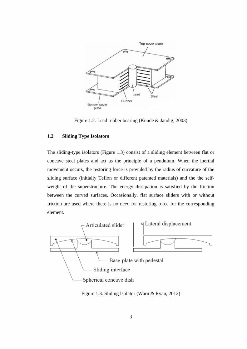
1.2 Sliding Type Isolators

The sliding-type isolators (Figure 1.3) consist of a sliding element between flat or

concave steel plates and act as the principle of a pendulum. When the inertial

movement occurs, the restoring force is provided by the radius of curvature of the

sliding surface (initially Teflon or different patented materials) and the the self-

weight of the superstructure. The energy dissipation is satisfied by the friction

between the curved surfaces. Occasionally, flat surface sliders with or without

friction are used where there is no need for restoring force for the corresponding

element.

Figure 1.3. Sliding Isolator (Warn & Ryan, 2012)

4

1.3 Development of SI in Turkey

In Turkey, as a seismically active country, SI applications have become popular in

2000's, especially after the amendment of Ministry of Health in 2013 obligating the

use of SI in hospitals with more than 100 beds and located in high seismic zones.

The specification includes limitations on target performance of the structure,

requirements on analysis and structural design, quality control and testing of

isolators. Later in 2019, the updated Turkish Building Seismic Code (TBDY2019)

was officially announced, including a performance-based design approach and base

isolation chapter. Since 2013, dozens of large hospital buildings have already been

constructed according to national and international codes (Erdik et al., 2018).

Furthermore, airport roofs, bridges, viaducts, data centers, residential, industrial and

storage buildings have been constructed, reaching a total of 104 isolated structures

until 2018, including the ones under the planning stage mentioned in Murota et al.

(2021). This number has been increasing rapidly since then. However, Erdik et al.

(2018) also mention the lack of facilities and experience in architectural,

engineering, production, testing and logistics aspects of a base isolation design in

Turkey.

1.4 Problem Statement

Isolated buildings have been designed using linear and nonlinear approaches. Recent

international codes (TBDY2019, ASCE7-16, Eurocode8, AASHTO) require

isolators to be preliminarily designed with linear analyses such as equivalent lateral

force approach or response spectrum analysis to evaluate maximum displacements

and structural forces. Then, nonlinear time history analyses (NTHA) are conducted,

and performance criteria are checked for both the isolation system and the

superstructure. Those performance parameters generally include maximum

displacements, structural forces, story accelerations, interstory drifts, isolator

hysteresis and uplift behavior.

5

In the analytical modeling stage, researchers and engineers tend to use different

mathematical models suggested by design codes or the literature to define the

hysteretic behavior of isolators for NTHA. These include bilinear models (sharp and

smoothed) and highly nonlinear models, which will be covered later in detail. The

bilinear models are more practical and can easily be implemented in the structural

analysis by following the design code guidelines. In contrast, nonlinear models

which accurately capture the actual behavior are more complex to implement and

require better comprehension of nonlinear dynamic isolator characteristics. These

models were used in both research and design projects. However, experience and

literature have shown that the characteristics of the hysteresis loops might introduce

significant variations in performance parameters.

1.5 The Aim and Research Objectives

The aim of this study is to assess the effect of the isolator modeling approach on

earthquake performance of 10 stories base-isolated reinforced concrete hospital

building, with plan irregularity, under a set of 11 ground motions. The structural

system consists primarily of beam-column frame elements. In addition, shear walls

are present at the core regions, which significantly affects the isolation system design

and evaluation. For the building, two types of isolation systems, HDRB, and double-

curved type FPS were designed and evaluated primarily according to the Turkish

seismic code (TBDY2019). In addition, international codes were also referenced

where needed. The reason behind selecting HDRB and FPS is that they both show

highly nonlinear responses under earthquake excitation. There is a sudden increase

in stiffness of HDRB under high shear strains, whereas the nonlinear restoring

stiffness of FPS type depends heavily on corresponding column axial load for which

strict bilinear relationship might not be observed for both types. However, the

findings of the research can also be partially applicable for LRB or other sliding-type

isolators, as the same nonlinear models can be used.

6

The objectives of this research are as follows:

• To observe the effect of isolator modeling approach on the structural

performance

• To highlight the advantages and drawbacks of each isolator model

encountered during the design and analysis.

1.6 The Outline of the Thesis

In Chapter 1, a brief introduction and history of SI isolator types are mentioned. The

research objectives are defined and a brief literature review regarding the objectives

are given.

Chapter 2 includes information on the building model and the design and different

modeling approaches of isolation elements.

In Chapter 3, seismic conditions of the building site, ground motion selection, and

nonlinear time history analysis approach are discussed.

The analysis results are presented in Chapter 4. Maximum displacements, structural

forces, story accelerations, inter-story drifts, hysteresis curves and uplift conditions

are evaluated for each isolator type and modeling approach. Performance

comparisons with code requirements are given.

Finally, Chapter 5 summarizes this study. Conclusions and recommendations are

discussed.

7

CHAPTER 1

2 LITERATURE REVIEW

In this chapter, the literature review of the topics which is covered in this thesis is

summarized. First, the nonlinear hysteresis models most often used by researchers

and engineers are addressed, including bilinear and other nonlinear models for

HDRB and FPS. Next, the studies, which focus on variation in structural

performance when one of these models is used, will be mentioned. In addition, the

uplift behavior of isolators are investigated.

2.1 Isolator Nonlinear Models

Adequacy of the force-displacement relationship of sharp bilinear (BL) models was

investigated in numerous studies and recommended (Robinson, 1982; Skinner et al.

1993; Kikuchi & Aiken, 1997, Kampas & Makris, 2012, Vassiliou et al. 2013).In

addition, international design codes besides Naeim and Kelly (1999) suggest all type

isolators can essentially be modeled by bilinear models. An illustration of force-

displacement relationship of the sharp BL model is shown in Figure 2.1 with the

dotted line. Three parameters are associated with this model: the initial elastic

stiffness, the characteristic strength and the post-yield (secondary) stiffness. A

secondary parameter, yield displacement, is optionally neglected in most cases due

to a small magnitude of elastic deformation of the isolator. A sharp and sudden

corner is provided between stiffness transitions, for which the effects on the response

will be discussed in the following chapters. After the maximum load in each cycle is

reached, the unloading curve follows a parallel line of the same length with the

previous loaded segments, in the opposite direction, until it reconnects the envelope

8

curve. The sharp bilinear model, which is implemented in the commercial structural

analysis programs as a link element, does not account for the bilateral excitation of

the ground motion components. In other words, the internal deformations are

uncoupled, and the deformation in a direction does not affect the motion in the

orthogonal direction (CSI Analysis Reference Manual, 2017).

Figure 2.1. Force-displacement relationship of BL (dotted line) and BW (solid line)

Another bilinear model, called as smoothed bilinear (or Bouc-Wen, BW) model,

was introduced by Bouc (1971) and modified by Wen (1976) and Park et al. (1986).

This analytical model can be applied to a wide range of hysteretic systems and was

verified for base isolation of a six-story reinforced concrete building by Nagarajaiah

et al. (1991) for both elastomeric and sliding isolators. In Figure 2.1 with solid line,

the hysteresis is defined by three parameters: elastic stiffness, the ratio of post-yield

stiffness to elastic stiffness, and the yield force. Unlike the sharp bilinear model, the

transition between initial and post-yield stiffness is smoothed by a circular yield

surface function, and the two lateral degrees of freedom are coupled. Therefore, the

model is able to capture nonlinear characteristics of isolators under biaxial lateral

excitation. The vertical degree of freedom is linearly elastic and uncoupled from the

9

horizontal directions. This model is implemented in ETABS software as Rubber

Isolator link element (CSI Analysis Reference Manual, 2017).

A nonlinear model which can be applicable for elastomeric isolators, specifically

HDRB, was developed by Kato et al. (2015) and validated by Masaki et al. (2017).

A time-independent "Deformation History Integral Type Model (DHI model)" can

accurately capture the highly nonlinear behavior of rubber bearings under biaxial and

uniaxial excitations. An elastoplastic model (DHI) was constructed by modifying

the viscoelastic models of Simo and Hughes (1997) since the velocity dependency

of restoring force was overestimated when compared by the HDRB test results in the

original one. Although the real rubber has velocity dependence, the DHI model does

not exhibit dependency on the strain rate. The characteristics of the hysteresis highly

depend on the shear strain and have stiffness increase when the shear strain exceeds

200%. This model is also implemented in ETABS, named as High Damping Rubber

Isolator Link (CSI Analysis Reference Manual, 2017). The axial behavior is linearly

elastic and independent from the two coupled shear directions. The following

parameters are required to define the DHI model. Isolator cross-sectional area,

isolator effective height, added elastic stiffness. which controls elastic region of the

response, hysteretic parameters (number of terms, control strain, and control

strength) which affects the hysteretic behavior, damage parameters which define the

damage function and elastic stiffness degradation (resistance ratio and control

strain); and finally, stiffness for iteration which might change the convergence rate

of the model.

10

Figure 2.2. Force-displacement relationship of HDRB (solid line) (retrieved from

Bridgestone Isolation Product Line-up)

Another highly nonlinear model can accurately capture the behavior of sliding

isolators, recommended by Nagarajaiah et al. (1991). This model is an advanced

model used both in research and practice and will be called as Friction Pendulum

Isolator (FPI) model in this study. The horizontal frictional hysteretic behavior is

based on the theory of smoothed bilinear model (Wen, 1976; Park et al., 1986). A

pendulum behavior was also added by Zayas and Low (1990). The axial behavior of

the model is always nonlinear, with a linear elastic compressive stiffness and zero

tensile stiffness. The horizontal force-deformation behavior of the isolator is the

same as the BW model, in Figure 2.1. Both shear directions are coupled with axial

behavior. When the axial load on the isolator increases, the restoring stiffness

increases, and lateral force also increases along with the frictional. The shear

behavior is velocity dependent, and two types of friction coefficient are introduced;

shear coefficient at fast velocities and zero velocity. Nagarajaiah et al. (1991) state

that the friction coefficient essentially increases with sliding velocity. To construct

the hysteresis loop, initial elastic stiffness, friction coefficient with zero and fast

velocities, the rate parameter which controls the rate of frictional change with the

velocity, and the radius of curvature are defined.

11

Some trilinear hysteretic models account for a higher degree of nonlinearity in the

isolators (Furukawa et al., 2005; Markou & Manolis, 2016). Furthermore, additional

models for triple friction pendulum bearings are also present (Fenz & Constantinou,

2008). However, these models are not a concern of this study.

2.2 Effect of Isolator Model on the Response

Studies mentioned in this section have shown that different analytical hysteretic

models of isolators may yield significant deviations in seismic response. Isolator

models, having sharper edges between stiffness transitions, tend to show higher

superstructural response. On the other hand, more accurate hysteretic and structural

responses could be achieved using smoothed or highly nonlinear models, which are

relatively more complex to implement in structural analysis.

Mavronicola and Komodromos (2014) conducted a series of analysis using 18 pulse-

like ground motions to compare sharp and smoothed (Bouc-Wen) bilinear models

for LRB isolators. Several cases were investigated in the parametric study; different

normalized characteristic strength, yield displacement of isolator, isolation period,

earthquake ground motion, and the number of stories (three and five stories). The

results showed that the maximum isolator relative displacements could be

overestimated or underestimated with the sharp bilinear model. Average

displacements do not significantly change with the isolation system characteristics

but were mostly influenced by the earthquake characteristics. However, seismic

response accelerations seem to be slightly increased when the sharp bilinear model

was used instead of a more accurate and smoothed model. which was attributed to

the contribution of higher modes and the abrupt change in the isolator stiffness. It

was also stated that the ratio of the characteristic (yield) strength to the seismic

weight on the isolator has considerable effects on the isolation system's behavior and

the superstructure.

12

In a Ph.D. dissertation thesis (Mavronicola, 2017), the discrepancies of the response

of sharply bilinear and smoothed bilinear models were investigated. 2-D analyses of

3 and 5 story base-isolated buildings with LRB were conducted under 50 pulse-like

ground motions. It was found that when the sharp bilinear model is used, computed

maximum floor acceleration and story drifts are overestimated. The deviation was

more significant when the isolation system has higher normalized characteristic

strength values. The displacement response for both models was comparable, and

sharp bilinear models can be used with confidence if appropriate safety factors are

included.

A commentary in ASCE7-16 (Chapter C17, C17.5.5) states that sharp bilinear

systems were observed to have higher floor accelerations and superstructural forces.

Therefore, it recommended a higher vertical force distribution factor in Equivalent

Lateral Force Procedure (ELFP) for the systems with sharper bilinear hysteresis,

basically for FPS. However, these findings were insufficiently developed to include

in the design guidelines.

Several hysteretic models were developed and compared with the experimental

results of triple friction pendulum isolators in Ray et al. (2013). The hysteresis

response of the isolator showed better agreement with test results when the stiffness

transition regions were modeled in a smoother manner, despite the fact that sharp

edges also showed acceptable compliance but were more susceptible to numerical

problems during the sudden stiffness transitions.

2.3 Tensile Behavior of Isolators

High rise structures, having shear walls, irregularities, and higher structural aspect

(height/width) ratio, may induce significant tensile (uplift) forces, especially on

corner isolators during a seismic action. Therefore, it is essential to comprehend the

tensile behavior and the capacity of the isolators during an earthquake event.

13

A parametric study was conducted on a four-story base-isolated steel building with

asymmetry and different isolators, vibration periods, damping ratio under various

ground motions, with and without vertical earthquake components (Koshnudian &

Motamendi, 2013). The study highlighted the importance of including the vertical

component of the earthquake in the analysis as overturning moments, beam shear

forces, corner column axial loads, and local uplifts could be significantly affected,

especially for structures with a high aspect ratio. On the other hand, it was shown

that the vertical component has negligible influence on system isolator hysteretic

response. Furthermore, several dynamic shake table test specimens with high aspect

ratio and having strong ground motion (Feng et al., 2004; Takaoka et al., 2011;

Masaki et al., 2000) show that although the isolation system was stable, isolators are

prone to tensile forces for buildings with such characteristics.

Novel research was conducted in Japanese literature on tensile behavior and capacity

of all rubber isolators during displaced positions (Kani et al., 1999; Iwabe et al.,

1999; Takayama et al., 1999). Moreover, a nonlinear tensile stiffness model and

deformation behavior were investigated by the test results up to 250% shear strain in

Yang et al. (2010). It is also mentioned that maximum tensile shear strains from 17%

up to 42% were observed in experimental studies for structures with different

characteristics. To avoid excessive tensile deformations and damage in the isolator,

the tensile strain was restricted to 5% of total rubber height in Japanese literature and

more than 1 MPa of tensile stress is not allowed in the Chinese design code.

An experimental study (Erkakan, 2014) was conducted on the isolation performance

of circular rubber bearings with different sizes and loading protocols during

horizontal deformation. The isolators were subjected to tensile stresses up to 2 MPa

and shear strain up to 100% without significant degradation in hysteretic parameters.

Also, it is mentioned that in the literature (Mano & Mangerig, 2018)., isolator limit

tensile stress value is often taken as 2𝐺𝑣 (where 𝐺𝑣 is the shear modulus of rubber)

and after this limit, the tensile stiffness of rubber isolators drops significantly due to

the cavitation damage.

14

If uplift in rubber bearings cannot be avoided, some bilinear or multi spring models

could be used to reflect the axial behavior accurately into the analytical model (Warn

& Ryan, 2012). In practice, the axial force-deformation relationship is often taken as

bilinear elastic, multiplying the compression stiffness by a reduction factor in order

to calculate tensile stiffness. In Pietra and Park (2017), 190 full-scale tests were

conducted on different isolator diameter and lead plug sizes. It was seen that when

working under 3𝐺𝑣 tensile stresses, the tensile post-yield stiffness degradation during

the cycles was not significant. It is also stated that lower bound cavitation occurred

when 10-12% tensile strains were reached, and acceptable cavitation limit loads were

specified between 2𝐺𝑣-3𝐺𝑣. Finally, the ratio of tensile stiffness to the compressive

stiffness was found to vary between 1/10 (for isolator of small diameter) to 1/80

(large diameter).

International design codes have different requirements about the uplift behavior in

rubber bearings. In ASCE7-16 (2016), local uplift of elements might be allowed if

the resulting deflections will not result in overstress or instability of the isolator. In

EN15129 (2009), it is mentioned that a tensile stresses up to 2𝐺𝑣 can be bearable

without significant cavitation; otherwise, uplift restraining connections are

recommended. California Department of Transportation (Caltrans, 2010) does not

allow uplift. Finally, TBDY2019 and AASHTO LRFD (2010) recommends tie-down

or anchorage systems to eliminate the uplift effect.

Conventional sliding isolators have no tensile carrying capability, and a gap is

generated between the upper and lower plates when the tensile load exceeds the

weight on the isolator during an earthquake due to the high vertical accelerations or

overturning. Therefore, no frictional restoring force is generated when the isolator is

in uplift condition. Similarly, very high compressive forces are also generated during

a seismic event, followed by the uplift, resulting in excessively high shear restoring

forces due to the friction action. Moreover, following the uplift of isolators, an

impact could happen between the sliding materials, which could significantly

damage sliding surfaces and the isolator and hysteretic behavior.

15

Although, so far, no reported real earthquake case of sliding isolator failure due to

uplift has been documented (Calvi & Calvi, 2018). several studies aim to observe

uplift behavior on sliding pendulum isolators understructures with high aspect ratio

and significant overturning.

Morgan (2007) conducted shaking table tests on quarter scale base-isolated steel

braced frame. The study highlighted the importance of variation of axial loads due

to overturning, and the aspect ratio (approximately 3:1) of the structure was selected

large enough to create uplift under selected ground motions. The stability of the

isolators was preserved after the tests where local uplift motions (not exceeding 0.25

seconds of disconnection of the plates) were observed. However, the isolators'

significant variations in axial forces were attained, diverging from a bilinear

hysteretic shape. These test results are compatible with Fenz's (2008) findings in

which double and triple friction pendulum isolators were dynamically tested to

facilitate practical implementation. In the study, approximately a magnitude of 2-3

mm of uplift displacements were observed for two cases; by the overturning and

rocking (isolator hitting the displacement restrainer) motions. For both cases,

instantaneous uplift behavior was observed, and upon contact of sliding surfaces,

isolators normally continued to their hysteretic motion without any problem. If such

a motion is observed, uplift magnitudes should be carefully assessed to prevent the

slider from toppling over the isolator and become unstable or resulting in structural

damage.

Uplift restrained devices were proposed and studied in many cases for the situations

where uplift demands are unbearable or unwanted for sliding isolators (Roussis &

Constantinou, 2006; Roussis, 2009; Kasalanati & Constantinou, 2005) and for rubber

isolators (Griffith et al., 1990). However, these systems are not investigated in the

concept of this thesis.

17

CHAPTER 2

3 ANALYTICAL MODEL

3.1 Building Model Information

The building is one of the 10-story T-shaped blocks of a base-isolated reinforced

concrete (RC) hospital which was built in a high seismic zone in Turkey. The

structural system consists mostly of column and beam (frame) elements and shear

walls supporting the core (elevators and stairs) regions to limit the lateral

displacements on the superstructure. The plan geometry is 115 m in the X direction

and 75 m in the orthogonal Y direction, and the total height is 40.9 m.

The pedestal sizes are 1250x1250 mm below the isolation layer. The column

dimensions are mostly 900x900 mm for the first floor and 800x800 mm for the upper

floors. Moreover, beam dimensions of 800x600 mm were used throughout the

structure. In addition, a limited number of columns and beams of different sizes were

also used in the structural system. The shear wall thickness is 300 mm everywhere.

Section rigidities of all members were modified by recommended values in Table

13.1 in TBDY2019 to account for cracking during the earthquake.

A 3-D structural model was created and analyzed using the commercial structural

analysis program ETABS (v18.1.1) (Figure 3.1. ), and the isolation layout is given

in Figure 3.2.

18

Figure 3.1. 3-D view of building model

Figure 3.2. Isolator plan layout

In addition to the self-weight of the reinforced-concrete structure, a uniform load of

3.92 kN/m2 of dead load (G) and 3.5 kN/m2 of live load (Q) were used throughout

the structure and on the top floor, 1 kN/ m2 of snow load, which was also included

as a live load, was used. The floor masses and the seismic mass of the structure from

the G+0.3Q loading condition are shown in Table 3.1. The first ten periods and total

mass participation ratios of the fixed base structure are given in Table 3.2. The first

mode period is 19 s, and coupling of the X and Y directions is observed.

19

Table 3.1 Story and structural masses

Story Mass

Floor 10 664

Floor 9 5307

Floor 8 4861

Floor 7 4862

Floor 6 4862

Floor 5 4803

Floor 4 4986

Floor 3 4909

Floor 2 5175

Floor 1 5374

Isolation 5142

Floor -1 1070

Tot. Str. Mass 52015

Table 3.2 Modes of fixed base structure

Mode Period Mx My

1 1.912 0.4480 0.1148

2 1.860 0.1003 0.5920

3 1.693 0.1481 0.0019

4 0.559 0.0339 0.0320

5 0.547 0.0265 0.0475

6 0.490 0.0260 0.0003

7 0.285 0.0089 0.0317

8 0.278 0.0201 0.0158

9 0.254 0.0003 0.0000

10 0.237 0.0207 0.0001

3.2 Seismicity and Selected Ground Motions

The building is located in a high seismic region in Turkey. The shear wave velocity

at 30 m depth of the soil, Vs30, was retrieved as 350 m/s. It corresponds to ZD soil

class in TBDY2019. MCE and DBE level elastic spectra were obtained from

Interactive Seismic Hazard Map (AFAD, Ministry of Interior of Turkey). In order to

conduct nonlinear time history analysis, eleven ground motions were selected from

PEER NGA-West2 Ground Motion Database (Pacific Earthquake Engineering

Research Center, University of California). The selected ground motions are scaled

so that the average accelerations of the ground motion spectra will not be less than

1.3 times the response spectra. The characteristics of the ground motions and their

scale factors for MCE and DBE are shown in Table 3.3. Comparison of acceleration

spectrum of each ground motion with the target spectra in Figure 3.3 and Figure 3.4

for MCE and DBE level seismic condition.

20

Figure 3.3. Target spectra and averaged spectra of eleven ground motions for MCE

Figure 3.4. Target spectra and averaged spectra of eleven ground motions for DBE

0

0.5

1

1.5

2

2.5

3

0 1 2 3 4 5 6

Sa

(g)

T (sec)

MCE

MCE_Target*1.3

Average

0

0.2

0.4

0.6

0.8

1

1.2

1.4

1.6

1.8

2

0 1 2 3 4 5 6

Sa

(g)

T (sec)

DBE

DBE_Target*1.3

Average

21

Table 3.3 Eleven ground motions and scale factors for MCE and DBE

An illustration of orthogonal lateral components of unscaled ground motions are

shown in Figure 3.5. Moreover, the unscaled ground motions with details and

vertical components are given in Appendix A.

Result

ID

Record

Seq. #

Tp-

PulseEvent Year Station

Magnit

ude

Mechani

sm

Vs30

(m/s)

MCE_

SF

DBE_

SF

1 187 - "Imperial Valley-06" 1979 "Parachute Test Site" 6.53 strike slip 348.7 3.892 2.404

2 316 4.389 "Westmorland" 1981 "Parachute Test Site" 5.9 strike slip 348.7 2.030 1.254

3 549 - "Chalfant Valley-02" 1986 "Bishop - LADWP South St" 6.19 strike slip 303.5 2.826 1.746

4 558 - "Chalfant Valley-02" 1986 "Zack Brothers Ranch" 6.19 strike slip 316.2 1.724 1.065

5 821 - "Erzican_ Turkey" 1992 "Erzincan" 6.69 strike slip 352.1 1.125 0.695

6 850 - "Landers" 1992 "Desert Hot Springs" 7.28 strike slip 359 3.530 2.180

7 1116 - "Kobe_ Japan" 1995 "Shin-Osaka" 6.9 strike slip 256 2.487 1.536

8 1158 - "Kocaeli_ Turkey" 1999 "Duzce" 7.51 strike slip 281.9 1.281 0.791

9 1605 - "Duzce_ Turkey" 1999 "Duzce" 7.14 strike slip 281.9 0.947 0.585

10 2752 - "Chi-Chi_ Taiwan-04" 1999 "CHY101" 6.2 strike slip 258.9 2.814 1.738

11 6893 - "Darfield_ New Zealand" 2010 "DFHS" 7 strike slip 344 1.517 0.937

22

Figure 3.5. Unscaled horizontal components of 11 ground motions

3.3 Isolator Design and Nonlinear Models

High damping rubber bearing and friction pendulum system type isolators were

designed for the structure to evaluate the rubber isolator performance. To assess the

effect of the analytical models for FPS and HDRB, various isolator models used by

researchers and designers were selected. First, the nonlinear time history analysis

was conducted using more advanced types, called Friction Pendulum Isolator (FPI)

and Deformation History Integral Type (DHI), respectively. Then, less accurate

bilinear models called smoothed Bouc-Wen Model (BW) and sharp bilinear model

(BL) were adopted for structural analyses.

23

TBDY2019 was used as the foremost guidelines during the design. Isolators to be

designed based on three load combinatioıns given below:

1.4𝐺 + 1.6𝑄 (3.1)

1.2𝐺 + 𝑄 ± 𝐸 (3.2)

0.9𝐺 ± 𝐸 (3.3)

Where 𝐺 is the dead load, 𝑄 is the live load, and 𝐸 is the effect of the earthquake, by

considering the combination of three ground motion components. In this case, the

earthquake loads were obtained by the average results of 11 ground motions from

nonlinear time history analyses. Several types for FPS and HDRB were constructed

according to their maximum compressive and tensile loads. The upper and lower

bound isolator properties recommended by the manufacturer were used. Design

criteria and stability checks in TBDY2019 (Section 14) were satisfied.

A preliminary design for the isolation system was conducted using Equivalent

Lateral Force Procedure (ELFP) according to TBDY2019. The displacement at an

earthquake level can be calculated by Eq (3.4). The subscript “𝑀” stands for the

MCE (DD-1) level earthquake, and thus, the equation could also be used for DBE

(DD-2) level earthquake by substituting the corresponding parameters.

𝐷𝑀 = 1.3 (𝑔

4𝜋2) 𝑇𝑀

2𝜂𝑀𝑆𝑎𝑒𝑀𝐶𝐸(𝑇𝑀)

(3.4)

Where, 𝑆𝑎𝑒𝑀𝐶𝐸(𝑇𝑀) is the spectral acceleration for the corresponding effective period,

𝑇𝑀 is the effective period of the structure and 𝜂𝑀 is the damping scale factor and 𝜉

is the damping ratio for the corresponding maximum displacement and calculated by

Eq (3.5) and Eq (3.6), respectively.

𝑇𝑀 = 2𝜋√𝑊

𝑔𝐾𝑀

(3.5)

24

𝜂𝑀 = √10

5 + 𝜉

(3.6)

Evaluation of the damping ratio (𝜉) often requires the target displacement of the

isolator. Therefore, since Eq (3.4) becomes an implicit equation, a step by step

iteration procedure was conducted by assuming an initial effective period and

damping ratio for each isolator type.

The maximum displacements should be increased, as shown in Eq (3.7), because of

the torsional movement of the isolation system. The movement, including torsion

(𝐷𝑇𝑀) shall not be less than the 1.1𝐷𝑀.

𝐷𝑇𝑀 = 𝐷𝑀 [1 + 𝑦12𝑒

𝑏2 + 𝑑2] ≥ 1.1𝐷𝑀

(3.7)

Where 𝑒 is the distance between the center of mass and the center of stiffness of the

isolation system, b and d are the two most extended dimensions of the structure.

The forces transferred to the superstructure can be calculated by Eq (3.8),

𝑉𝑀 =𝑆𝑎𝑒𝑀𝐶𝐸(𝑇𝑀)𝑊𝜂𝑀

𝑅

(3.8)

Where 𝑊 is the structural weight (G+0.3Q), and 𝑅 is the structural behavior factor

(taken as equal to one) affecting the ductility demand on the superstructure. More

realistic structural forces can also be obtained by using the ELFP in ASCE7-16,

which removes the weight of the isolation slab from the superstructure and can

redistribute the lateral forces to the superstructure. In the end, higher superstructural

forces were obtained when ASCE7-16 is used.

25

3.3.1 Design of High Damping Rubber Bearings

The preliminary isolation system design, having a target period of 3 s and damping

ratio of 20%, was conducted according to the equivalent lateral force procedure

(ELFP) (TBDY2019 Section14.14.2 ). The lower and upper bounds were taken as

0.9 and 1.45 respectively, recommended by Bridgestone and applied in the analysis

according to TBDY2019 (Section 14.12). The summary table for the ELFP using

both MCE and DBE level earthquakes with nominal, upper, and lower bound

properties is shown in Table 3.4. The isolation system yielded 416 mm maximum

displacement in MCE level ground motion with LB properties. Also, the forces,

11.4% and 12.4% of seismic weight, are transferred to the superstructure in DBE UB

properties in TBDY2019 and ASCE7-16.

Table 3.4 Equivalent lateral force procedure for HDRB

Analysis Type

MCE-

LB

MCE-

Nom

MCE-

UB

DBE-

LB

DBE-

Nom

DBE-

UB

Seismic Weight (kN) 𝑊 499727

Effective Period (s) 𝑇𝑀 2.942 2.765 2.208 2.510 2.326 1.774

Damping Ratio % 𝜉 22% 22% 23% 24% 24% 24%

Total Effective

Stiffness (kN/m)

𝐾𝑀 232429 263189 412514 319363 371929 639180

Damping Scale

Factor

𝜂𝑀 0.610 0.606 0.594 0.587 0.587 0.535

Spectral Acc. (g) 𝑆𝑎𝑒(𝑇𝑀) 0.222 0.236 0.295 0.151 0.163 0.214

Max. Displ. (m) 𝐷𝑀 0.378 0.353 0.276 0.181 0.167 0.116

Max. Disp. w/

Torsion (m)

𝐷𝑇𝑀 0.416 0.388 0.304 0.199 0.184 0.128

TBDY2019 Base

Shear (Vm/W)

0.135 0.143 0.175 0.089 0.096 0.114

ASCE7-16 Base

Shear (Vm/W)

0.143 0.152 0.186 0.095 0.102 0.124

26

In a collaborative research project with Bridgestone Corporation (Japan), four types

of HDRB (Bridgestone Seismic Isolation Product Line-up, 2017) were selected for

the building. According to their maximum earthquake compressive loads (Eq (3.1)),

the isolators were grouped into four categories. The tensile capacity recommended

by Bridgestone and other papers (Mano & Mangerig, 2018; EN15129, 2009, Pietra

& Park, 2017), 1 MPa was adopted. Isolators that exceeded the tensile capacity were

moved into the greater size to reduce the stresses.

The design was conducted based on an isolation system having a maximum of 200%

shear strain displacements, dictated by TBDY2019, under maximum earthquake

level (MCE); despite the fact that it was observed HDRB isolators could undergo

higher strain limits up to 300% shear strains without any significant deterioration in

hysteresis loops (Kikuchi & Aiken, 1997; Masaki et al., 2017). Therefore, isolator

total rubber height is selected as 200 mm, which corresponds nearly 210% shear

strain. The code limitation is exceeded by a little in this situation. However, HDRB

has a increasing nonlinear stiffness at shear strains higher than 200-250%, and

hysteresis loops of some ground motions with higher shear strains can now be

observable.

It should be noted that the periods DBE-UB and DBE-Nom conditions are close to

the fixed base structure period. Therefore, relatively higher superstructural response

might be expected when the evaluation is conducted.

A table including HDRB properties and design loads is presented in Table 3.5. The

vertical compression stiffnesses of the isolators were calculated according to

TBDY2019 (Appendix 14A).

27

Table 3.5 HDRB isolator design loads and properties

Type 1 Type 2 Type 3 Type 4

# of isolator # 57 36 25 17

Average Seismic

Weight (kN) G+0.3Qave 1649 4036 6099 6352

Maximum Static Load

(kN) 1.4G+1.6Qmax 6646 9777 12024 12362

Maximum Earthquake

Load (kN) 1.2G+Q+Emax 9000 12000 15000 17174

Minimum Eathquake

Load (Tension) (kN) 0.9-Emax 580 737 915 958

Shear Modulus (kPa) Gv 620 620 620 620

Elastic Modulus (4*Gv)

(kPa) E0 2480 2480 2480 2480

Coefficient on Hardness k 0.6 0.6 0.6 0.6

Comp. Modulus (kPa) Ec 4003547 3702695 3711696 3812646

Bulk Modulus (kPa) K 2000000 2000000 2000000 2000000

Vertical Rigidity

Modulus (kPa) Ev 1333727 1298577 1299683 1311845

Vertical Rigidity

(kN/m) Kv 4283139 5058781 6166376 7402727

Outer Diameter (m) Do (B) 0.9 1 1.1 1.2

Inner Diameter (m) Di (BL) 0.02 0.055 0.055 0.055

Effective Area (m2) Ar 0.6359 0.7830 0.9480 1.1286

28

Table 3.5 (Cont’d) HDRB isolator design loads and properties

Inner Area (m2) Ai 0.000 0.002 0.002 0.002

Rubber layer thickness

(m) tr 0.006 0.0067 0.0074 0.008

Number of Layers n 33 30 27 25

Tot. Rubber Height (m) H 0.198 0.201 0.200 0.200

Tot. Iso. Height (m) Ht 0.4108 0.4006 0.3902 0.3856

First Shape Factor S1 36.7 35.3 35.3 35.8

Second Shape Factor S2 4.55 4.98 5.51 6.00

Max. Rubber Elong. εb 5 5 5 5

Design Rotation Angle

(rad) θs 0.005 0.005 0.005 0.005

Using the mechanical characteristics in Table 3.4. the bilinear shear properties were

obtained by the equations of Bridgestone recommendation. (Bridgestone Product

Isolation Line-up, 2017). It was seen that the results from the Bridgestone equations

are compatible with the equations used in TBDY2019 for rubber isolators. The

equivalent shear modulus 𝐺𝑒𝑞, damping ratio 𝐻𝑒𝑞, and a function of a ratio of

characteristic strength to the maximum force 𝑢 should be calculated first to obtain

equivalent stiffness 𝐾𝑒𝑞, initial stiffness 𝐾1, post-yield stiffness 𝐾2, and characteristic

(yield) strength stiffness 𝑄𝑑. The expressions for these parameters are shown from

Eq (3.9) to Eq (3.15).

29

𝐺𝑒𝑞(𝛾) = 0.620(0.1364𝛾4 − 1.016𝛾3 + 2.903𝛾2 − 3.878𝛾

+ 2.855)

(3.9)

𝐻𝑒𝑞(𝛾) = 0.240𝑥(0.02902𝛾3 − 0.1804𝛾2 + 0.2364𝛾 + 0.9150) (3.10)

𝑢(𝛾) = 0.408𝑥(0.03421𝛾3 − 0.2083𝛾2 + 0.2711𝛾 + 0.9028 (3.11)

𝐾𝑒𝑞 = 𝐺𝑒𝑞𝐴𝑟/𝐻

(3.12)

𝐾2 = 𝐾𝑒𝑞(1 − 𝑢)

(3.13)

𝐾1 = 10𝑥𝐾2

(3.14)

𝑄𝑑 = 𝑢𝐾𝑒𝑞𝐻 𝛾 (3.15)

The corresponding shear properties of isolators were determined from the equations

above for nominal properties. The secondary rigidity and characteristic strength are

multiplied by LB or UB factors when necessary. The lateral shear properties of four

isolator types for MCE and DBE conditions are given from Table 3.6 to Table 3.11.

Table 3.6 Isolator bilinear properties for MCE-LB condition


γ 1.469 1.447 1.455 1.454

𝑫𝒎 (m) 0.291 0.291 0.291 0.291

𝑮𝒆𝒒 (kPa) 519 522 521 521

𝑯𝒆𝒒 (ξ) % 0.232 0.232 0.232 0.232

𝒖 0.392 0.393 0.392 0.392

𝑲𝒆𝒒 (kN/m) 1500 1830 2224 2646

𝑲𝟐 (kN/m) 913 1111 1351 1607

𝑲𝟏 (kN/m) 8787 10659 12982 15440

𝑸𝒅 (kN) 192.5 237.0 286.9 341.6

𝑭𝒎𝒂𝒙 (kN) 524.6 646.1 782.2 931.2

30

Table 3.7 Isolator bilinear properties for MCE-Nom condition


γ 1.370 1.349 1.357 1.356

𝑫𝒎 (m) 0.271 0.271 0.271 0.271

𝑮𝒆𝒒 (kPa) 533 536 534 535

𝑯𝒆𝒒 (ξ) % 0.234 0.234 0.234 0.234

𝒖 0.396 0.397 0.397 0.397

𝑲𝒆𝒒 (kN/m) 1710 2087 2535 3017

𝑲𝟐 (kN/m) 1032 1258 1529 1819

𝑲𝟏 (kN/m) 10324 12580 15293 18195

𝑸𝒅 (kN) 183.8 224.7 272.8 324.7

𝑭𝒎𝒂𝒙 (kN) 463.7 565.9 687.5 818.1

Table 3.8 Isolator bilinear properties for MCE-UB condition


γ 1.072 1.056 1.063 1.062

𝑫𝒎 (m) 0.212 0.212 0.212 0.212

𝑮𝒆𝒒 (kPa) 597 601 600 600

𝑯𝒆𝒒 (ξ) % 0.239 0.239 0.239 0.239

𝒖 0.406 0.407 0.407 0.407

𝑲𝒆𝒒 (kN/m) 2778 3398 4124 4908

𝑲𝟐 (kN/m) 1649 2015 2447 2912

𝑲𝟏 (kN/m) 16489 20154 24472 29121

𝑸𝒅 (kN) 239.7 293.4 356.1 423.8

𝑭𝒎𝒂𝒙 (kN) 589.8 721.3 875.6 1042.0

31

Table 3.9 Isolator bilinear properties for DBE-LB condition


γ 0.702 0.692 0.696 0.695

𝑫𝒎 (m) 0.139 0.139 0.139 0.139

𝑮𝒆𝒒 (kPa) 772 779 776 777

𝑯𝒆𝒒 (ξ) % 0.241 0.240 0.240 0.240

𝒖 0.409 0.409 0.409 0.409

𝑲𝒆𝒒 (kN/m) 2231 2731 3314 3944

𝑲𝟐 (kN/m) 1318 1615 1959 2332

𝑲𝟏 (kN/m) 13184 16148 19592 23317

𝑸𝒅 (kN) 126.8 155.2 188.4 224.2

𝑭𝒎𝒂𝒙 (kN) 310.1 379.7 460.7 548.3

Table 3.10 Isolator bilinear properties for DBE-Nom condition


γ 0.651 0.641 0.645 0.644

𝑫𝒎 (m) 0.129 0.129 0.129 0.129

𝑮𝒆𝒒 (kPa) 809 817 814 814

𝑯𝒆𝒒 (ξ) % 0.240 0.240 0.240 0.240

𝒖 0.408 0.408 0.408 0.408

𝑲𝒆𝒒 (kN/m) 2599 3182 3861 4595

𝑲𝟐 (kN/m) 1538 1884 2286 2720

𝑲𝟏 (kN/m) 15382 18839 22857 27202

𝑸𝒅 (kN) 136.7 167.3 203.0 241.6

𝑭𝒎𝒂𝒙 (kN) 334.8 409.9 497.4 592.0

32

Table 3.11 Isolator bilinear properties for DBE-UB condition


γ 0.497 0.489 0.492 0.492

𝑫𝒎 (m) 0.098 0.098 0.098 0.098

𝑮𝒆𝒒 (kPa) 948 956 953 953

𝑯𝒆𝒒 (ξ) % 0.238 0.238 0.238 0.238

𝒖 0.404 0.404 0.404 0.404

𝑲𝒆𝒒 (kN/m) 4415 5399 6554 7800

𝑲𝟐 (kN/m) 2631 3219 3907 4650

𝑲𝟏 (kN/m) 26310 32192 39073 46499

𝑸𝒅 (kN) 175.3 214.3 260.2 309.7

𝑭𝒎𝒂𝒙 (kN) 434.0 530.8 644.4 766.8

3.3.1.1 Deformation History Integral Type (DHI) Model

One elastic spring and two hysteretic springs were included in the DHI model. The

concept is shown in Figure 3.6. The resulting hysteresis is the sum of all hysteretic

springs in the model. This model is shear strain-dependent, and the stress-strain

mathematical expression is given in Eq (3.16).

The two horizontal directions are coupled; therefore, the DHI model can capture a

highly nonlinear response under bilateral excitations. The horizontal stiffness

significantly increases after 200% shear strain for HDRB, contributing to the total

system damping. This behavior cannot be accurately captured in other bilinear

models unless comprehensive modifications are made.

33

Figure 3.6. DHI model concept, elastic and hysteretic spring behavior (Eser et al.

2020)

𝜏𝑥(𝛾𝑥, 𝛾𝑦) = Ξ(𝑡)𝐺𝑒𝛾𝑥 +∑𝑔𝑖∫ 𝑒−(𝛤−𝛤′)/𝑙𝑖

𝑑

𝑑𝛤′[1

3(𝛾𝑥

′ − 𝛾𝑥)(𝛾𝑥′2 + 𝛾𝑦

′ 2) + 𝛾𝑥′] 𝑑𝛤′

𝛤

0

𝑛

𝑖

(3.16) 𝜏𝑦(𝛾𝑥, 𝛾𝑦) = Ξ(𝑡)𝐺𝑒𝛾𝑦 +∑𝑔𝑖∫ 𝑒−(𝛤−𝛤′)/𝑙𝑖

𝑑

𝑑𝛤′[1

3(𝛾𝑦

′ − 𝛾𝑦)(𝛾𝑥′2 + 𝛾𝑦

′ 2) + 𝛾𝑦′ ] 𝑑𝛤′

𝛤

0

𝑛

𝑖

Ξ(𝑡) = 𝜃 + (1 − 𝜃) exp (−𝛾𝑚(𝑡)

𝛾𝑑)

where,

𝛤 = ∫ √𝑑𝛾𝑥2 + 𝑑𝛾𝑦2𝐶

𝛾𝑚(𝑡) = max𝑡[√𝛾𝑥2 + 𝛾𝑦2]

𝛾𝑥, 𝛾𝑦 : shear strain in x, y direction

𝜏𝑥, 𝜏𝑦 : shear stress in x, y direction

𝛤 : curvilinear integral along the deformation orbit C on 𝛾𝑥-𝛾𝑦 plane

𝑙𝑖, 𝑔𝑖, 𝐺𝑒 , 𝜃, 𝛾𝑑 : material parameters

Ξ(𝑡) : damage function (degradation of stiffness by loading history)

34

Horizontal material hysteretic control parameters, recommended by Bridgestone are

given in Table 3.12, and defined in ETABS in “High Damping Rubber Isolator” link

property, separately for upper and lower bound analyses.

Please note that these parameters were constructed by using the test data and the

“Added Elastic Stiffness, Ge” does not directly represents the the stiffness of the

isolator but only have effect on the elastic term. Therefore the nominal value of Ge

can be lower than the lower bound.

Table 3.12 Material input parameters for DHI model

Property Nominal UB LB

Added Elastic Stiffness – Ge (MPa) 0.5257 0.8136 0.5262

Control Strength 1 - g1 (MPa) 2.468 3.364 1.999

Control Strength 2 - g2 (MPa) 0.3564 0.4858 0.2887

Control Strain 1 - l1 0.03591 0.03591 0.03591

Control Strain 2 - l2 0.5 0.5 0.5

Resistance Ratio - θ 0.4598 0.4598 0.4598

Damage Parameter – γd 0.4181 0.4181 0.4181

The axial behavior is only linear elastic in high damping rubber isolator link

definition. Therefore, to account for different tensile and compressive behavior a

Multilinear Elastic” link element (CSI Analysis Reference Manual, 2017), having

only axial spring behavior definition, was also added in series to the horizontal

springs. The tensile stiffness was taken as 1/30 times of the compression stiffness for

all types (Pietra & Park, 2017). Axial force-displacement relationships for all four

types are presented in Figure 3.7. If the axial displacements exceed the maximum

displacement in the graph, a linear interpolation is applied in the model.

35

Figure 3.7. Axial force-displacement relationship of HDRB types

3.3.1.2 Smoothed Bouc-Wen (BW) Model

In this model, biaxial excitation of isolation elements can be captured accurately.

The axial and horizontal behaviors are uncoupled. The axial behavior is only linear

elastic; therefore the same multilinear axial links were assigned as in the DHI model

(Figure 3.7). For horizontal degrees of freedom, the biaxial diagram showing the

plasticity model implemented in ETABS is shown in Figure 3.8. The nonlinear shear

force-displacement behavior is governed by the relationships below for two

directions (𝑑𝑢2 and 𝑑𝑢3):

-5000

-4000

-3000

-2000

-1000

0

1000

-0.001 -0.0005 0 0.0005 0.001 0.0015 0.002 0.0025 0.003

Axia

l F

orc

e (k

N)

Axial Displacement (m)

Type 1

Type 2

Type 3

Type 4

36

Figure 3.8. The isolator property definition for biaxial deformation (retrieved from

CSI Analysis Reference Manual, 2017)

𝑓𝑢2 = 𝑟𝑎𝑡𝑖𝑜2𝑘2𝑑𝑢2 + (1 − 𝑟𝑎𝑡𝑖𝑜2)𝑦𝑖𝑒𝑙𝑑2𝑧2

(3.17)

𝑓𝑢3 = 𝑟𝑎𝑡𝑖𝑜3𝑘3𝑑𝑢3 + (1 − 𝑟𝑎𝑡𝑖𝑜3)𝑦𝑖𝑒𝑙𝑑3𝑧3

(3.18)

Where, 𝑘2 and 𝑘3 are the initial elastic stiffness, 𝑟𝑎𝑡𝑖𝑜2 and 𝑟𝑎𝑡𝑖𝑜3 are the ratio of

post-yield stiffness to initial stiffness, 𝑦𝑖𝑒𝑙𝑑2 and 𝑦𝑖𝑒𝑙𝑑3 are the yield (characteristic)

force of the isolator. 𝑧2 and 𝑧3are the internal hysteretic variables. The range of the

variables are in the range of √𝑧22 + 𝑧3

2 ≤ 1, outside of the yield region and

√𝑧22 + 𝑧3

2 = 1, circular shape at the yield surface. The value of the hysteretic

parameters are defined according to following implicit differential equations and

having a zero value at initial conditions. The relation (Eq (3.19)) was constructed by

using the dimensionless quantities that control the shape of the hysteresis in Park et

al. (1986) with 𝐴 = 1 and 𝛽 = 𝛾 = 0.5.

37

{𝑧2̇𝑧3̇} = [

1 − 𝑎2𝑧22 −𝑎3𝑧2𝑧3

−𝑎2𝑧2𝑧3 1 − 𝑎3𝑧32]

{

𝑘2

𝑦𝑖𝑒𝑙𝑑2𝑑𝑢2̇

𝑘3𝑦𝑖𝑒𝑙𝑑3

𝑑𝑢3̇ }

(3.19)

Where,

𝑎2 = {1 𝑖𝑓 𝑑𝑢2𝑧2 > 0̇

0 𝑜𝑡ℎ𝑒𝑟𝑤𝑖𝑠𝑒

(3.20)

𝑎3 = {1 𝑖𝑓 𝑑𝑢3𝑧3 > 0̇


(3.21)

According to Bridgestone recommendations, the bilinear hysteretic characteristics of

HDRB isolators were calculated using mechanical isolator properties and presented

in Table 3.6, Table 3.10 and Table 3.11. The rubber isolator input parameters were

extracted from the bilinear shear properties of the isolators and are presented in Table

3.13 for MCE-LB, DBE-UB, and DBE-Nom analyses, that are used for structural

response evaluation.

Table 3.13 Smoothed bilinear model input parameters

MCE-

LB

DBE-

Nom

DBE-

UB

Type

1

keff2,3 1500 2599 4415

k2,3 9127 15382 26310

yield2,3 171 137 175

ratio2,3 0.1

Type

2

keff2,3 1830 3182 5399

k2,3 11110 18839 32192

yield2,3 209 167 214

ratio2,3 0.1

Type

3

keff2,3 2224 3861 6554

k2,3 13512 22857 39073

yield2,3 254 203 260

ratio2,3 0.1

Type

4

keff2,3 2646 4595 7800

k2,3 16075 27202 46499

yield2,3 302 242 310

ratio2,3 0.1

38

3.3.1.3 Sharp Bilinear (BL) Model

In this model, all three degrees of freedom are uncoupled. The envelope curve of

the nonlinear force-displacement relationship is directly the input parameter for axial

and two shear deformations. This model is implemented in ETABS as the

“Multilinear Plastic (MLP) Link” property, and the “Kinematic Hysteresis Model”

was used as the energy dissipating mechanism. The concept of the model for each

independent direction is shown in Figure 3.9.

Figure 3.9. Sharp bilinear concept

The sharp bilinear characteristics were estimated from bilinear shear properties from

Table 3.6, Table 3.10 and Table 3.11 and are shown in a graphical form from Figure

3.10 to Figure 3.12 for MCE-LB, DBE-Nom, and DBE-UB cases. The nonlinear

axial behavior can be modeled similarly to the shear directions. Different

compressive and tensile stiffnesses were assigned as in DHI model, Figure 3.7.

39

Figure 3.10. HDRB sharp bilinear envelope input for MCE-LB isolator properties

Figure 3.11. HDRB sharp bilinear envelope input for DBE-Nom isolator properties

40

Figure 3.12. HDRB sharp bilinear envelope input for DBE-UB isolator properties

3.3.2 Design of Friction Pendulum System

Double curved surface frictional sliders may be used in the design of the building.

The friction pendulum system consists of an articulated frictional disk that slides

between concave plates. The damping is provided by the friction and the restoring

stiffness is achieved by the curvature of the surfaces and the gravity. The friction is

load-dependent and varies with the sliding velocity and temperature. During an

earthquake, due to the variation of axial column loads, the restoring stiffness shows

high nonlinearity, especially in locations with higher overturning moments and shear

walls. In most cases, isolators located at the corner regions of buildings and shear

walls exhibit uplift behavior due to the axial load variation. Since friction pendulum

isolators do not have tensile carrying mechanisms, no frictional force is generated

during the uplift.

The preliminary analysis with ELFP was conducted with a target period of 3.5 s and

20% damping in MCE level seismic input with lower bound isolator properties. Due

to the variation in friction coefficient related to aging, testing and production

41

variation, the lower and upper bound parameters are taken as 0.9 and 1.56,

respectively, and applied in the analysis according to TBDY2019 (Section 14.13).

Maximum displacement with torsional effects was calculated as 0.502 m. The base

shear forces were attained as 10.7% and 11.6% of superstructural weight for

TBDY2019 and ASCE7-16, respectively. The summary table for ELFP analysis for

all isolator properties is given in Table 3.14.

A friction pendulum system was designed according to TBDY2019 guidelines.

Preliminarily, the isolators were grouped into three types depending on their

maximum compressive loads. The nominal effective dynamic friction coefficient is

selected as 5.5% and the radius of curvature as 4.5 m. The maximum uplift

displacements will be examined in Chapter 5 and compared with the literature.

Table 3.14 Equivalent lateral force procedure for FPS

Analysis Type

MCE-

LB

MCE-

Nom

MCE-

UB

DBE-

LB

DBE-

Nom

DBE-

UB

Seismic Weight (kN) 𝑊 499727

Effective Period (s) 𝑇𝑀 3.488 3.378 2.874 2.883 2.459 1.897

Damping Ratio % 𝜉 21% 24% 30% 30% 30% 30%

Effective Stiffness

(kN/m)

𝐾𝑀 165289 176202 243426 241936 332616 558692

Damping Scale

Factor

𝜂𝑀 0.621 0.592 0.535 0.535 0.535 0.535

Spectral Acc. (g) 𝑆𝑎𝑒(𝑇𝑀) 0.187 0.193 0.227 0.132 0.154 0.200

Max. Displ. (m) 𝐷𝑀 0.456 0.422 0.324 0.189 0.161 0.125

Max. Disp. w/

Torsion (m)

𝐷𝑇𝑀 0.502 0.464 0.356 0.208 0.177 0.137

TBDY2018 Base

Shear (Vm/W)

0.116 0.114 0.121 0.070 0.083 0.107

ASCE7-16 Base

Shear (Vm/W)

0.123 0.122 0.131 0.076 0.089 0.116

42

The bilinear properties were obtained using the equations below, retrieved from

TBDY2019 (Appendix 14B) and shown in Table 3.15 for MCE and Table 3.16 for

DBE level seismic conditions.

𝐹𝑄 = 𝐹𝑦 = 𝜇𝑒𝑃 (3.22)

𝑘2 =𝑃

𝑅𝑐

(3.23)

𝑘𝑒 =𝐹

𝐷=𝑃

𝑅𝑐+𝜇𝑒𝑃

𝐷

(3.24)

𝛽𝑒 =1

2𝜋[𝑊𝑑

𝐹𝐷] =

2

𝜋[

𝜇𝑒𝜇𝑒 + 𝐷/𝑅𝐶

] (3.25)

Table 3.15 FPS isolator characteristics for MCE level seismic condition

MCE-LB MCE-Nom MCE-UB

𝜇𝑒 0.0495 0.055 0.0858

𝑅𝐶 m 4.5 4.5 4.5

𝐷 m 0.351 0.325 0.249

𝐹𝑦,𝑡𝑜𝑡𝑎𝑙 kN 24736 27485 42877

𝑘2,𝑡𝑜𝑡𝑎𝑙 kN/m 111050 111050 111050

𝑘1,𝑡𝑜𝑡𝑎𝑙 = 100𝑘2 kN/m 11105044 11105044 11105044

𝑘𝑒,𝑡𝑜𝑡𝑎𝑙 kN/m 181558 195747 283139

𝐹𝑚𝑎𝑥,𝑡𝑜𝑡𝑎𝑙 kN 63697 63522 70545

𝛽𝑒 % 25% 28% 30%

𝑇𝑒𝑓𝑓 s 3.328 3.205 2.665

𝜔 rad 0.3005 0.3120 0.3752

43

Table 3.16 FPS isolator characteristics for DBE level seismic condition

DBE-LB DBE-Nom DBE-UB

𝜇𝑒 0.0495 0.055 0.0858

𝑅𝐶 m 4.5 4.5 4.5

𝐷 m 0.145 0.124 0.096

𝐹𝑦,𝑡𝑜𝑡𝑎𝑙 kN 24736 27485 42877

𝑘2,𝑡𝑜𝑡𝑎𝑙 kN/m 111050 111050 111050

𝑘1,𝑡𝑜𝑡𝑎𝑙 = 100𝑘2 kN/m 11105044 11105044 11105044

𝑘𝑒,𝑡𝑜𝑡𝑎𝑙 kN/m 281201 332620 558736

𝐹𝑚𝑎𝑥,𝑡𝑜𝑡𝑎𝑙 kN 40881 41260 53512

𝛽𝑒 % 30% 30% 30%

𝑇𝑒𝑓𝑓 s 2.674 2.459 1.897

𝜔 rad 0.3739 0.4067 0.5271

3.3.2.1 Friction Pendulum Isolator (FPI) Model

The plasticity model of Park et al. (1986) was adopted for the shear behavior, and

the pendulum behavior is added by Zayas and Low (1990). The axial force is always

nonlinear and have significant affects on the shear behavior (CSI Analysis Reference

Manual, 2017).

The concept is shown in Figure 3.13. All three degrees of freedom are coupled. The

nonlinear axial force-deformation behavior is defined with compression stiffness and

zero tensile stiffness, Eq (3.26). The frictional and pendulum force deformation

behavior are given in Eq (3.28) and Eq (3.29), respectively. Frictional behavior is

highly affected by the variation in nonlinear axial load during an earthquake.

44

Figure 3.13. FPI model concept (retrieved from CSI Analysis Reference Manual,

2017)

𝑓𝑢1 = 𝑃 = {𝒌𝟏𝑑𝑢1 𝑖𝑓 𝑑𝑢1 < 00 𝑜𝑡ℎ𝑒𝑟𝑤𝑖𝑠𝑒

(3.26)

𝑓𝑢2,3 =𝑓𝑢2,3𝑓 + 𝑓𝑢2,3𝑝𝑓𝑟𝑖𝑐𝑡𝑖𝑜𝑛 𝑝𝑒𝑛𝑑𝑢𝑙𝑢𝑚

The frictional force-deformation relationship is given by:

(3.27)

𝑓𝑢2,3𝑓 = −𝑃𝜇2,3𝑧2,3 (3.28)

𝜇2,3 = 𝒇𝒂𝒔𝒕𝟐,𝟑 − (𝒇𝒂𝒔𝒕𝟐,𝟑 − 𝒔𝒍𝒐𝒘𝟐,𝟑)𝑒−𝑟𝑣 (3.29)

The comma notation is used to separate the directions in the terms in order not to

show the same equations again. Where, 𝑠𝑙𝑜𝑤2,3 are the friction coefficients at zero

velocity, and 𝑓𝑎𝑠𝑡2,3 are the friction coefficients at fast velocities in corresponding

horizontal direction (2 or 3). The friction coefficient is normally increases with

sliding velocity for Teflon-steel materials (Nagarajaiah et al,1991). The resultant

velocity is denoted as 𝑣. The 𝑟 is an effective inverse velocity and characterized by

inverse of characteristic sliding velocities, 𝑟𝑎𝑡𝑒2,3.

45

𝑣 = √�̇�𝑢2,32 + �̇�𝑢3,2

2

𝑟 =𝒓𝒂𝒕𝒆𝟐,𝟑 �̇�𝑢2,3

2 + 𝒓𝒂𝒕𝒆𝟑,𝟐�̇�𝑢3,22

𝑣2

𝑧2,3 are the internal hysteretic variables. The range of the variables was in the range

of √𝑧22 + 𝑧3

2 ≤ 1 outside of the yield region, and √𝑧22 + 𝑧3

2 = 1, circular shape at

the yield surface. The value of the hysteretic parameters are defined according to

following implicit differential equations and having a zero value at initial conditions.

The relation (Eq (3.30)) were constructed by using the dimensionless quantities that

control the shape of the hysteresis in Park et al. (1986) with 𝐴 = 1 and 𝛽 = 𝛾 =

0.5.

{𝑧2̇𝑧3̇} = [

1 − 𝑎2𝑧22 −𝑎3𝑧2𝑧3

−𝑎2𝑧2𝑧3 1 − 𝑎3𝑧32]

{

𝒌𝟐𝑃𝜇𝑢2

𝑑𝑢2̇

𝒌𝟑𝜇𝑢2

𝑑𝑢3̇ }

(3.30)

Where, 𝑘2 and 𝑘3 are the initial elastic shear stiffnesses and,

𝑎2 = {1 𝑖𝑓 𝑑𝑢2𝑧2 > 0̇


𝑎3 = {1 𝑖𝑓 𝑑𝑢3𝑧3 > 0̇


The pendulum force-deformation relationship is given below. 𝒓𝒂𝒅𝒊𝒖𝒔𝟐 and

𝒓𝒂𝒅𝒊𝒖𝒔𝟑 are the effective radius of curvature (pendulum length) of the sliding

surface. Generally, the radius of curvature and friction coefficients are the same for

both shear directions.

𝑓𝑢2,3𝑝 = −𝑃𝑑𝑢2,3

𝒓𝒂𝒅𝒊𝒖𝒔𝟐,𝟑

46

The input parameters that are bolded in previous equations were introduced to the

analysis program. These are axial compression stiffness, elastic shear stiffness,

friction coefficients at zero and fast velocities, rate parameter and pendulum radius.

Used parameters are given in Table 3.17, Table 3.18 and Table 3.19, for MCE-LB,

DBE-Nom, and DBE-UB level analyses.

Table 3.17 FPI model input parameters for MCE-LB

Type 1 Type 2 Type 3

k2,3 40872 113327 141448

slow2,3 0.0396 0.0396 0.0396

fast2,3 0.0495 0.0495 0.0495

rate2,3 1

radius2,3 4.5

Table 3.18 FPI model input parameters for DBE-Nom


k2,3 40872 113327 141448

slow2,3 0.0440 0.0440 0.0440

fast2,3 0.0550 0.0550 0.0550

rate2,3 1

radius2,3 4.5

Table 3.19 FPI model input parameters for DBE-UB


k2,3 40872 113327 141448

slow2,3 0.0686 0.0686 0.0686

fast2,3 0.0858 0.0858 0.0858

rate2,3 40872

radius2,3 4.5

47

3.3.2.2 Sharp Bilinear (BL) Model

The same sharp bilinear model used as Section 3.3.1.3 was also adopted for FPS

isolators. This is a model used by many engineers who are inexperienced of the

nonlinear concept of the nonlinear frictional behavior of sliding isolators. Although,

FPS has coupled degrees of freedom in all directions, in BL model all three directions

are independent from each other.

The bilinear concept is presented in Figure 3.14. Bilinear properties were obtained

from Table 3.15, and Table 3.16, and hysteresis envelope input are constructued and

shown from Figure 3.15, Figure 3.16, and Figure 3.17. The axial force-deformation

relationship of each type is shown in Figure 3.18.

Figure 3.14. Sharp bilinear concept

48

Figure 3.15. FPS sharp bilinear envelope input for MCE-LB isolator properties

Figure 3.16. FPS sharp bilinear envelope input for DBE-Nom isolator properties

49

Figure 3.17. FPS sharp bilinear envelope input for DBE-UB isolator properties

Figure 3.18. FPS sharp bilinear axial load-deformation input

-2500000

-2000000

-1500000

-1000000

-500000

0

500000

-0.25 -0.20 -0.15 -0.10 -0.05 0.00 0.05 0.10 0.15 0.20 0.25

Axia

l F

orc

e (k

N)

Axial Deformation (m)

Type1

Type2

Type3

51

CHAPTER 3

4 NONLINEAR TIME HISTORY ANALYSIS

This chapter covers nonlinear time-history analysis, which was used to assess the

structural performance of selected isolator models under selected seismic

excitations. Fast Nonlinear Analysis (FNA), i.e., Nonlinear Modal Time-History

Analysis (Ibrahimbegovic & Wilson, 1989; Wilson, 1993), was chosen due to its

efficiency compared to the Direct Integration method. The method is implemented

in ETABS. First, the theoretical background of the FNA method is discussed. Later,

ETABS load case implementation and selected analysis options for eleven ground

motions are explained.

4.1 Fast Nonlinear Analysis (FNA)

The response of structures under considerable dynamic input shows significant

nonlinear behavior. These nonlinearities generally include P-delta effects and

nonlinear material properties. For the response history analysis of linear and

nonlinear systems, N. M. Newmark (1959) developed a family of methods, known

as “direct time-integration methods”. In the direct integration method, the complete

equilibrium equations are formed and solved at each time step. Solving the nonlinear

behavior of elements throughout the structure using the direct integration method

may require enormous analysis time, in the magnitudes of hours/days, especially for

relatively larger real-scale buildings.

E. L. Wilson (2000) proposed an analysis method for structures having a limited

number of nonlinear elements, such as base isolators, dampers and gap elements.

This new method is called Fast Nonlinear Analysis (FNA) and can reduce analysis

duration significantly.

52

In FNA method, fundamental equations of mechanics (equilibrium, force-

deformation and compatibility) are satisfied. The matrix equation of motion at time

(t) is given in Eq (4.1),

𝐌�̈�(𝑡) + 𝑪�̇�(𝑡) + 𝑲𝐿𝒖(𝑡) + 𝑹(𝑡)𝑁𝐿 = 𝑹(𝑡) (4.1)

Where 𝐌, 𝑪, and 𝑲𝑳 are the mass, damping and the linear effective stiffness matrices,

respectively. The size of the matrices is equal to the number of degrees of freedom

for the corresponding node. �̈�(𝑡), �̇�(𝑡), 𝒖(𝑡) and 𝑹(𝑡) are the nodal point

acceleration, velocity, displacement, and externally applied load (seismic

excitation), respectively. 𝑹(𝑡)𝑁𝐿 is the vectorial sum of the forces in nonlinear elements

and is computed by iteration at each step.

There are cases when the computer model becomes unstable without the nonlinear

elements. In this case, the linear effective stiffness, 𝑲𝑵𝑳 of the nonlinear elements

can be added, and Eq (4.1) can be rewritten as the following equation.

𝐌�̈�(𝑡) + 𝑪�̇�(𝑡) + (𝑲𝑳 +𝑲𝑵𝑳)𝒖(𝑡) = 𝑹(𝑡) − 𝑹𝑁𝐿(𝑡) + 𝑲𝑵𝑳𝒖(𝑡) (4.2)

The effective stiffness at nonlinear degrees of freedom (𝑲𝑵𝑳) is arbitrary; however,

it varies between zero and maximum nonlinear stiffness of the corresponding degree

of freedom. Also, the exact dynamic equilibrium equations for the model can be

written as:

𝐌�̈�(𝑡) + 𝑪�̇�(𝑡) + 𝑲𝒖(𝑡) = �̅�(𝑡) (4.3)

Where 𝑲 is the elastic stiffness matrix and is equal to 𝑲𝑳 +𝑲𝑵𝑳. The effective external

load �̅�(𝑡) is equal to 𝑹(𝑡) − 𝑹(𝑡)𝑁 +𝑲𝑵𝒖(𝑡), and evaluated by iteration. The

convergence rate of the solution can be increased by a reasonable estimation of the

effective elastic stiffness.

53

Modal analysis is conducted using the stiffness matrix 𝑲. and the mass matrix 𝐌.

The ritz vector method for the solution of the modal equations is recommended by

CSI (CSI Analysis Reference Manual, 2017).

The equilibrium equations are written in modal form as:

Ω2𝐚(t) + 𝛬�̇�(t) + 𝑰�̈�(t) = 𝒒(𝑡) − 𝒒𝑒(𝑡) (4.4)

The modal equations are shown from Eq (4.5) to Eq (4.10). Where, Ω2 is the diagonal

matrix of squared structural frequencies. 𝛬 is the modal damping matrix which is

diagonal. 𝑰 is the identity matrix which satisfies Eq (4.7), 𝒒(𝑡) is the vector of modal

applied loads, and 𝒒𝑁(𝑡) is the vector of modal forces from nonlinear elements (links),

and a(t) is the amplitude of modal deformations.

Ω2 = ΦT𝑲Φ (4.5)

𝛬 = ΦT𝑪 Φ (4.6)

𝑰 = ΦT𝑴Φ (4.7)

𝒒(𝑡) = ΦT𝑹(𝑡) (4.8)

𝒒𝑵(𝑡) = ΦT[𝑹𝑁𝐿(𝑡) − 𝑲𝑁𝒖(𝑡)] (4.9)

𝒖(𝑡) = Φ𝐚(t)

(4.10)

In the above equations, Φ is the mode shape. It should be noted that since 𝒒𝑵(𝑡) is a

function of modal amplitude 𝐚(t), unlike linear dynamic analysis, the modal equations are

coupled. In Ritz vector modal analysis, 500 modes were used and, 100% mass participation

in each direction were achieved.

54

Knowing the damping ratio in the structural system is also crucial to construct the damping

matrix. In a 3-D analysis, the nonlinear behavior of the isolators will include hysteretic

damping during the lateral deformation for the corresponding first three modes and the

superstructure will remain linear elastic with no energy dissipation. Also, it is widely

accepted that reinforced concrete structures have a damping ratio of 5% during a seismic

motion (Chopra, 2012; Pant et al., 2013). Therefore, since additional damping is not desired

in the isolation system’s dominant modes, a small damping ratio 0.5% is assigned to the first

three modes for all load cases. Zero damping ratio is avoided to prevent numerical problems.

Damping in all other modes (superstructural modes) is kept constant at 5% for the RC

structure.

Since the inter-story drifts of the building were yielded close to 0.5%, no cracking is

expected in the concrete. Therefore 5% damping might not be satisfied in base-isolated

cases. For this reason, a comparison of superstructural response for 5% and 2% damping is

given in Appendix D. as an additional analysis. For the 2% damping case, higher

accelerations are obtained while inter-story drifts remain similar.

As a validation for the FNA analysis, additional analyses using Newmark’s DI method for

specified earthquakes were conducted and compared in terms of hysteresis curves and

superstructural response. The results are given in Appendix E. The hysteresis response is

compatible with both methods. However, Higher superstructural responses (accelerations

and story drifts) up to 10% were obtained with selected DHI and MLP modeling approaches,

except enormously amplified accelerations at Floor 2 are observed when the DI method is

used. The convergence of the solution could not be satisfied when the FPI model is analyzed

by the direct integration method due to the negative and zero stiffnesses during the uplift

movements (CSI Analysis Reference Manual, 2017).

55

4.2 Load Case Implementation

Load case definitions for 3-D nonlinear time-history analyses were constructed for 11

ground motions, presented in Section 0, separately with the scale factors for DBE and MCE

level earthquakes. The FNA method is selected for the solution. All three components of the

ground motions were assigned according to guidelines in TBDY2019.

To account for the static loading conditions before the earthquake excitation, the structural

weight (G+0.3Q) was applied as the nonlinear initial condition for all load cases. The seismic

weight was administered with a ramp-shaped loading function that reached a total unity

amplitude with a 20 s duration. This is important, especially for frictional sliding isolators.

If there is zero compression load on the isolator as an initial condition, no initial horizontal

stiffness is generated; therefore, the convergence of the solution cannot be achieved at the

beginning of the analysis. The structural stiffness is recomputed after the application of the

service loads, and tridirectional seismic excitation begins with modified stiffnesses.

Two orthogonal horizontal components of the ground motions were introduced in the

analysis program with the same scale factors. For each ground motion, two sets of load cases

were defined by interchanging the orthogonal components of the acceleration history. A total

of 22 load cases were used in the analysis. The results of each ground motion are obtained

by considering the maximum response in each set. The final structural response was

evaluated by taking the average of the related parameter of 11 ground motions.

The vertical component was also included in each load case since the period of the dominant

vertical mode (0.149 s) was found to be more than 0.1 s (TBDY2019). The scale factor was

used the same as the lateral ones.

56

CHAPTER 4

5 RESPONSE OF ISOLATED HOSPITAL BUILDING

In this chapter, the response of both the isolation system and the superstructure is

assessed. The evaluation of response is conducted by obtaining the average results

of eleven ground motions. The hysteresis curves and the axial response of the links

were considered separately for several ground motions. The isolation system and

structural performance was evaluated according to maximum displacements,

structural forces and base shear coefficient, floor accelerations, inter-story drifts, and

hysteretic curves.

5.1 Maximum Isolation Displacements

Time history displacement response in both lateral directions was obtained for each

MCE ground motion with lower bound parameters. The horizontal displacements

were directionally combined at each time step. The average results of the eleven

ground motions were used to determine maximum displacement. Maximum

displacements were increased by %10, the minimum value, in this case, to account

for additional rotational effects.

A rigid first-floor slab, i.e., isolation mat, acts as a constraint for the top isolator

nodes; therefore, no relative lateral displacements are expected during a translational

displacement. However, due to the asymmetric plan of the building rotational

movements are present. Therefore, three different locations, which are the center of

the building, right-wing corner, and bottom wing corner, on the isolation system

were selected to observe the relative displacements throughout the structure. The

location of the isolators is shown on the isolator layout in Figure 5.1.

57

Figure 5.1. Selected isolator locations for system displacement response (the

isolator layout is retrieved from ETABS plugin by Ulker Eng.)

The orbital displacement response of each selected location is evaluated for each

HDRB model, and the average of maximum displacements from eleven ground

motions are plotted on the graphs. Also, maximum values of three selected locations

are given to assess additional displacements due to torsion.

Ux-Uy displacement response of all ground motions for the HDRB models are

shown from Figure 5.2 to Figure 5.4. Also, the maximum direction displacement of

each ground motion and their average are presented in Table 5.1. Average maximum

combined displacements for the DHI, smoothed BW, and sharp BL models were

gathered as 36.3, 36.2, and 35.0 cm, respectively. When the displacements are

increased by 10% for torsional effects, they are obtained as 39.9, 39.8, and 38.5 cm.

The ELFP method yielded maximum displacements as 37.8 and 41.6 cm with and

without torsion, respectively. The least displacements were obtained from sharp BL

models, with an 8% decrease from the preliminary ELFP analysis.

Excessive deformations are observed in the ground motions RSN316 (Westmorland,

1981) and RSN821 (Erzincan, 1992), which have pulse-like behavior and near-fault

effects in the records. In ground motion, RSN316, 61.3, 61.2, and 64.8 cm

58

displacements are observed for DHI, BW, and BL models, respectively. In this case,

the BL model yielded the maximum deformations. Furthermore, the displacements

are obtained very close to each other for different models in RSN850. Therefore,

there is no regular pattern in isolation system displacements for different HDRB

modeling approaches. Although the average displacements are close to each other,

the displacement response could be underestimated or overestimated with bilinear

models when the ground motions are evaluated separately. The deformation response

of the system is highly dependent also on the seismic input characteristics.

Table 5.1 Maximum displacements of HDRB models (units are in cm)

Eq ID Bottom Middle Right Bottom Middle Right Bottom Middle Right

RSN0187 37.61 36.91 41.51 37.51 36.82 41.47 43.85 42.86 45.09

RSN0316 58.23 58.36 61.32 57.97 58.13 61.22 64.07 64.09 64.79

RSN0549 24.73 23.28 25.68 24.63 23.20 25.63 18.21 17.95 20.23

RSN0558 20.28 19.69 20.02 20.22 19.64 19.99 18.66 17.79 18.05

RSN0821 47.16 48.07 47.44 47.00 47.93 47.35 54.12 53.95 55.21

RSN0850 21.34 20.56 20.45 21.25 20.48 20.41 21.17 20.85 20.80

RSN1116 31.32 31.33 31.25 31.17 31.20 31.21 28.57 28.41 26.50

RSN1158 41.24 40.54 42.63 41.04 40.38 42.55 36.73 36.39 38.09

RSN1605 44.27 44.54 44.58 44.11 44.40 44.51 38.93 40.02 40.35

RSN2752 33.50 33.04 33.02 33.36 32.92 32.94 35.30 35.52 35.52

RSN6893 29.69 30.03 31.23 29.59 29.94 31.20 19.36 19.45 20.44

AVE 35.40 35.12 36.28 35.26 35.00 36.22 34.45 34.30 35.01

Dm

Dtm 39.91 39.84 38.51

DHI Model BW Model BL Model

36.28 36.22 35.01

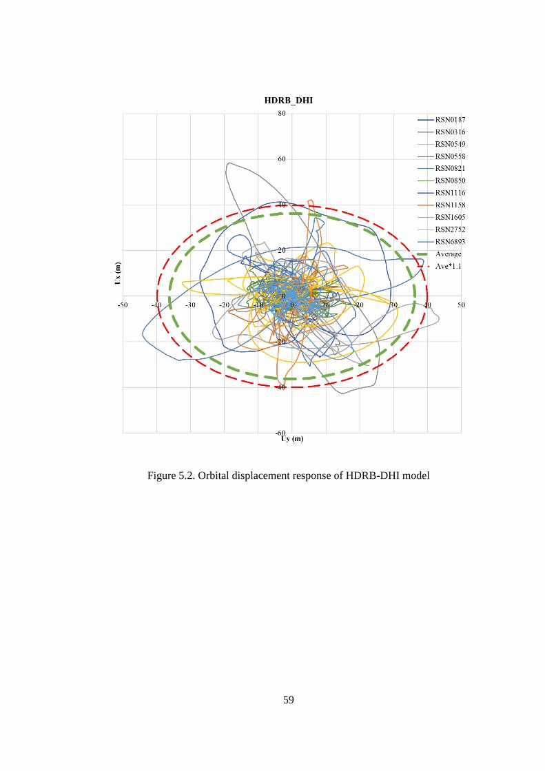
59

Figure 5.2. Orbital displacement response of HDRB-DHI model

60

Figure 5.3. Orbital displacement response of HDRB-BW model

61

Figure 5.4. Orbital displacement response of HDRB-BL model

62

The displacement responses of FPS models are shown in Figure 5.5 and Figure 5.6

for FPI and BL cases. Also, the maximum direction displacement of each ground

motion and their average are presented in Table 5.2. The tables showed average

maximum direction displacements for FPI and sharp BL models as 42.4 and 35.9

cm, respectively. When increased by torsion, 46.6 and 39.5 cm displacements were

obtained.

Table 5.2 Maximum displacement comparison of FPS models (units are in cm)

FPI Model BL Model

Eq ID Bottom Middle Right Bottom Middle Right

RSN0187 48.10 46.80 47.70 46.71 45.54 47.19

RSN0316 81.80 81.94 83.42 66.62 66.86 62.50

RSN0549 22.43 22.34 22.66 17.35 16.52 15.05

RSN0558 16.88 17.22 17.05 16.58 16.47 16.53

RSN0821 48.84 49.23 48.91 51.86 50.19 51.90

RSN0850 20.30 19.74 20.05 17.29 15.16 15.05

RSN1116 31.24 31.13 30.89 28.38 27.97 26.67

RSN1158 50.47 50.62 50.28 44.63 44.57 44.94

RSN1605 62.63 61.91 61.42 43.31 43.87 43.97

RSN2752 49.88 50.17 50.32 39.78 38.67 38.55

RSN6893 32.10 32.48 33.37 22.08 22.47 23.30

AVE 42.24 42.14 42.37 35.87 35.30 35.06

Dm 42.37 35.87

Dm*1.1 46.61 39.46

63

Figure 5.5. Orbital displacement response of FPS-FPI model

64

Figure 5.6. Orbital displacement response of FPS-BL model

65

The energy damping and nonlinear stiffness properties are prone to change during

uplift movements in an ideal condition, especially for sliding isolators. Also, in the

models which can account for biaxial excitation of the ground motion, displacements

in one direction affect the other degree of freedom. Since the sharp BL model always

follows the specified path and does not compute biaxial excitation, there is no

variation of stiffnesses or displacements due to the previous comments. This might

lead to maximum displacements that are less or higher than more realistic models.

The characteristics of the ground motion is also significant. These results are suitable

with the findings of Mavronicola and Komodromos (2014).

There is a small difference, a maximum of %7, in the displacement response of

different parts of the structure. Depending on the ground motion Bottom, Middle, or

Right locations showed higher or similar results than others with no pattern.

5.2 Structural Forces

The story forces and base shear reaction above the isolation layer are evaluated in

this section. The story forces at the bottom of the floors were obtained for each

isolator model in DBE seismic level with upper bound isolator properties. The

average forces for the eleven ground motions were calculated. Then the forces were

normalized with the structural weight. The story force distribution is plotted on the

graphs separately for HDRB and FPS designs. In the charts, floor numbers are

defined in the Y-axis. Floor -1 is the basement floor. The isolators are located at

Floor 0, and the first floor just above the isolation mat is Floor 1. The results show

that story forces are generally increased when the smooth BW and sharp BL models

were used instead of more accurate nonlinear models such as DHI and FPI.

For HDRB isolators, the average story force distributions in X and Y directions are

shown in Figure 5.7 and Figure 5.8, respectively. These results are observed to be

increased in X direction when bilinear models are used. The BW model showed

slightly lower story shear forces in the first four floors in Y direction. Among the

66

models, the sharp BL model yielded significantly higher demands for the structure.

Smoothed BW model was shown more compatibility with the DHI model, especially

at the higher floors.

When the average forces for MCE level earthquake is assessed in Figure 5.9 and

Figure 5.10, the BW model yielded slightly lower forces than DHI, especially for the

first floors. Therefore, the estimation of the BW model might change when different

earthquake level is applied. The reason might be attributed to the stiffness increase

after 200% shear strain for the DHI model, resulting in higher forces. On the other

hand, the BL model always results in the highest response. However, the difference

are more insignificant compared to the results with DBE level analysis.

The force demands showing the distribution for each earthquake are given from

Figure 5.11 to Figure 5.16 for the HDRB models for in both directions. There is an

amplification of the forces in the DHI models in Floor 1, especially for earthquakes

with higher scale factors or pulse-like characteristics. Similar graphs can also be

drawn for BL and BW models.

67

Figure 5.7. Story forces for HDRB models in the X direction with DBE-UB

parameters

Figure 5.8. Story forces for HDRB models in the Y direction with DBE-UB

parameters

-1

0

1

2

3

4

5

6

7

8

9

10

11

0 0.05 0.1 0.15 0.2

Flo

or

Story Force/Str Weight (V/W)

X-direction-HDRB-DBE

HDRB_DHI

HDRB_BW

HDRB_BL

-1

0

1

2

3

4

5

6

7

8

9

10

11

0 0.05 0.1 0.15 0.2

Flo

or


Y-direction-HDRB-DBE

HDRB_DHI

HDRB_BW

HDRB_BL

68

Figure 5.9. Story forces for HDRB models in X direction with MCE-LB

parameters

Figure 5.10. Story forces for HDRB models in Y direction with MCE-LB

parameters

-1

0

1

2

3

4

5

6

7

8

9

10

11

0 0.05 0.1 0.15 0.2

Flo

or


X-direction-HDRB-MCE

HDRB_DHI

HDRB_BW

HDRB_BL

-1

0

1

2

3

4

5

6

7

8

9

10

11

0 0.05 0.1 0.15 0.2

Flo

or


Y-direction-HDRB-MCE

HDRB_DHI

HDRB_BW

HDRB_BL

69

Figure 5.11. Story forces of each motion for HDRB-DHI model in X direction with

DBE-UB parameters

Figure 5.12. Story forces of each motion for HDRB-DHI model in Y direction with

DBE-UB parameters

70

Figure 5.13. Story forces of each motion for HDRB-BW model in X direction with

DBE-UB parameters

Figure 5.14. Story forces of each motion for HDRB-BW model in Y direction with

DBE-UB parameters

71

Figure 5.15. Story forces of each motion for HDRB-BL model in X direction with

DBE-UB parameters

Figure 5.16. Story forces of each motion for HDRB-BL model in Y direction with

DBE-UB parameters

72

For FPS isolators, the average story force distributions in X and Y directions are

shown in Figure 5.17 and Figure 5.18, respectively. There is significant

overestimation of the response when sharp BL model is used. The force distribution

for each earthquake is given from Figure 5.21 to Figure 5.34 for the FPS models for

DBE-UB conditions. In some of the ground motions, amplification of the forces at

Floor 1 is significant for both models, especially in the X direction.

The average forces for MCE level earthquake is assessed in Figure 5.19 and Figure

5.20. This time, lower demands are attained from BL for the first three stories, and

higher for the upper stories. During a seismic motion for the FPI model, shear forces

on the isolators, located nearby the shear walls, increases enormously for small

amount of time due to the high axial load dependency. It might have effects on the

absolute peak response. This phenomenon cannot be observed in the BL model since

axial and lateral degrees of freedom are not coupled.

73


DBE-UB parameters


DBE-UB parameters

-10123456789

1011

0 0.02 0.04 0.06 0.08 0.1 0.12 0.14

Flo

or


X-direction-FPS-DBE

FPS_FPI

FPS_BL

-10123456789

1011

0 0.02 0.04 0.06 0.08 0.1 0.12 0.14

Flo

or

Story Force/Str Weighr (V/W)

Y-direction-FPS-DBE

FPS_FPI

FPS_BL

74


MCE-LB parameters


MCE-LB parameters

-1

0

1

2

3

4

5

6

7

8

9

10

11

0 0.05 0.1 0.15

Flo

or


X-direction-FPS-MCE

FPS_FPI

FPS_BL

-10123456789

1011

0 0.05 0.1 0.15

Flo

or


Y-direction-FPS-MCE

FPS_FPI

FPS_BL

75

Figure 5.21. Story forces of each motion for FPS-FPI model in the X direction with

DBE-UB parameters

Figure 5.22. Story forces of each motion for FPS-FPI model in Y direction with

DBE-UB parameters

76

Figure 5.23. Story forces of each motion for FPS-BL model in X direction with

DBE-UB parameters

Figure 5.24. Story forces of each motion for FPS-BL model in Y direction with

DBE-UB parameters

77

The average base shear coefficients (V/W) for HDRB models under DBE-UB

parameters are compared in Table 5.3. From the bottom of the first floor, the shear

forces transferred to the superstructure (V/W) are 13.0% and 12.4% of the structural

weight for the DHI model for X and Y directions, respectively. When the bilinear

models are used, the results are overestimated by approximately 10% and 20% for

BW and BL models, respectively.

The average base shear coefficients for FPS models are compared in Table 5.4. The

forces transferred to the superstructure are obtained as 10.6% and 9.9% of the

structural weight for the FPI model for the two directions, respectively. The

corresponding results were overestimated and obtained as 11.8% and 11.5% by the

BL model.

Table 5.3 Average base shear coefficient comparison of HDRB models

W=499727 Vx/W Vy/W

DHI 0.130 0.124

BW 0.141 0.136

BL 0.160 0.151

Table 5.4 Average base shear coefficient comparison of FPS models in X-dir

W=499727 Vx/W Vy/W

FPI 0.106 0.099

BL 0.118 0.115

78

5.3 Story Accelerations

The maximum floor accelerations for each earthquake were obtained from the

analysis program, and the average of 11 ground motions was calculated. As specified

in TBDY2019, the resulting accelerations were evaluated from the design basis

earthquake (DBE) results with nominal isolator properties. The results are shown in

graphical forms. First floor is located at 0.00 elevation in the figures, and the

isolation level is at -4.5 m. The basement floor where pedestal columns are present

is located at -4.50 m elevation. The average of the peak ground accelerations of

eleven ground motions is approximately observed on the basement floor.

Due to the contribution of the higher modes, it was observed that the accelerations

could significantly increase in the upper floors. Özdemir (2010) and Erdik et al.

(2018) states that relatively tall and flexible structures on the isolators may

experience relatively higher floor accelerations.

Figure 5.25 and Figure 5.26 compare the average of maximum floor accelerations of

11 ground motions for HDRB models in the X and Y directions, respectively. The

DHI model yielded the lowest accelerations. Nearly 0.2 g until Floor 8 and 0.27 on

Floors 9 and 10. Therefore the results of the DHI model are less than 0.3 g on all

floors and satisfy the performance criteria. It is followed by the smooth BW model

of up to 30% higher response than the DHI. The sharp BL model yields the highest

response and shows significant amplification on the isolation floor.

79

Figure 5.25. Ave. floor accelerations of eleven motions for HDRB in X direction

Figure 5.26. Ave. floor accelerations of eleven motions for HDRB in Y direction

Figure 5.27 and Figure 5.28 compare the average of maximum floor accelerations of

11 ground motions for FPS models in the X and Y directions, respectively. The FPI

model resulted in accelerations between 0.27 g and 0.37 g in the first nine floors and

increased to 0.44 g on the top floor. Moreover, the sharp BL model showed results

up to 40% higher than the FPI model. Similar to the HDRB-BL model, acceleration

-10

0

10

20

30

40

50

0 0.1 0.2 0.3 0.4 0.5

Flo

or

Hei

gh

t (m

)

Floor Acceleration (g)

X-direction-HDRB-DBE-Nom

HDRB_DHI HDRB_BW HDRB_BL

-10

0

10

20

30

40

50

0 0.1 0.2 0.3 0.4 0.5 0.6

Flo

or

Hei

gh

t (m

)


Y-direction-HDRB-DBE-Nom


80

amplification was observed on -4.5 m elevation (isolation floor) in most ground

motions.

Figure 5.27. Ave. floor accelerations of eleven motions for FPS in X direction

Figure 5.28. Ave. floor accelerations of eleven motions for HDRB in Y direction

-10

0

10

20

30

40

50

0 0.1 0.2 0.3 0.4 0.5 0.6 0.7

Flo

or

Hei

gh

t (m

)


X-direction-FPS-DBE-Nom

FPS_FPI FPS_BL

-10

0

10

20

30

40

50

0 0.2 0.4 0.6 0.8

Flo

or

Hei

gh

t (m

)


Y-direction-FPS-DBE-Nom

FPS_FPI FPS_BL

81

The differences in the acceleration results are noticeable when idealized bilinear

models are adopted instead of more accurate nonlinear models. As an additional

example, analysis results of MCE level earthquakes with lower bound isolator

parameters are investigated. The average acceleration results from MCE-LB are

presented in Figure 5.29 and Figure 5.30 for both directions. Accelerations on the

isolation level decrease in MCE analysis as one expects from an isolation system.

However, the sharp BL model still shows significantly higher responses.

For this building, relatively high accelerations are obtained. In an isolated building,

one can expect isolation floor accelerations are closer to the base shear coefficient,

i.e. 10-12% in this study. However, there is more than one reason for this problem.

First, DBE isolator periods of both designs are close to the fixed-based period.

Optimization in the FPS design could allow the isolation system to be flexible and

to obtain a less structural response. On the other hand, the shear strain and uplift

limitations for HDRB isolators reduce the design alternatives and might result in a

costly rubber isolation system.

Second, especially for FPS isolators, a higher damping ratio in DBE conditions might

be associated with activation of the higher modes which yields higher superstructural

response (Warn & Ryan, 2012). These can also be combined with the sharp stiffness

transitions in BL models, also activating the higher modes (Mavronicola, 2017).

Another reason is that the structure is not symmetrical and more slender at the corner

locations and prone to significant demands under bilateral excitation. It is

investigated in a previous study with the same model but different earthquakes.

Three different locations from the building were selected and average accelerations

of 7 ground motions are compared under a DHI-DBE-Nom model with the maximum

results. The results are given in Appendix B. The locations far from the structural

center and at more slender regions experience higher accelerations and become

dominant when the peak accelerations are obtained from the software.

82

Figure 5.29. Ave. floor accelerations of eleven motions for MCE in X direction

Figure 5.30. Ave. floor accelerations of eleven motions for MCE in Y direction

-10

0

10

20

30

40

50

0 0.1 0.2 0.3 0.4 0.5 0.6 0.7 0.8

Flo

or

Hei

gh

t (m

)


X-direction-MCE-LB


FPS_FPI FPS_BL

-10

0

10

20

30

40

50

0 0.1 0.2 0.3 0.4 0.5 0.6 0.7 0.8 0.9

Flo

or

hei

gh

t (m

)


Y-direction-MCE-LB


FPS_FPI FPS_BL

83

Average accelerations from different elevations of the building are compared. The

top floor, isolation floor and peak ground accelerations (PGA) of HDRB models are

given in Table 5.5. The BW model estimates the accelerations approximately %35

higher than the DHI model. On the other hand, the increase in BL model is between

65-70% when compared the DHI model. On the isolation floor, the sharp BL model

yielded values higher than the PGA.

Table 5.5 Ave. accelerations of the top floor, isolation floor, and the PGA for HDRB

Average

Acc (g)

DHI BW BL

X Y X Y X Y

Top floor 0.277 0.293 0.377 0.393 0.461 0.487

Iso floor 0.233 0.245 0.313 0.320 0.392 0.418

PGA 0.380

The top floor, isolation floor and peak ground accelerations of FPS models are shown

in Table 5.6. The sharp BL model shows increased accelerations by 20- 30% when

compared to the FPI model. The FPI model yields accelerations that are close to the

PGA in both top and isolation floors.

Table 5.6 Ave. accelerations of the top floor, isolation floor, and the PGA for FPS

Average

Acc (g)

FPI BL

X Y X Y

Top

floor 0.438 0.553 0.583 0.688

Iso floor 0.361 0.391 0.430 0.518

PGA 0.380

84

5.4 Inter-story Drifts

To compare the inter-story drifts, maximum story drifts were obtained under DBE

seismic level with nominal isolator properties. The average of the maximum values

for each floor was calculated to assess according to the TBDY2019. In the code, the

superstructural drifts shall be below 0.005 drift ratio for non-structural damage

limitation.

For each HDRB model, the average inter-story drift ratio is shown in Figure 5.31

and Figure 5.32, for X and Y directions, respectively. The DHI model resulted in

least drifts less than 0.55 % for all stories. Furthermore, there is an approximately

10% higher story drift in the BW when compared to the DHI model. Also, the highest

drifts were attained in BL model, nearly 20% higher than the DHI. From the figures,

it can be seen that the bilinear models could overestimate the response significantly.

For the selected FPS isolator models, the superstructural drift response is introduced

in Figure 5.33 and Figure 5.34 for X and Y directions, respectively. Similar to the

HDRB case, the isolator model that induces higher nonlinearity in the hysteresis of

FPI brought lower response. When the sharp BL model is used, an overestimation in

the response is observed in all floors.

85

Figure 5.31. Ave. story drifts of eleven motions for FPS in X direction

Figure 5.32. Ave. story drifts of eleven motions for HDRB in Y direction

0

5

10

15

20

25

30

35

40

45

0 0.002 0.004 0.006 0.008 0.01

Flo

or

Hei

gh

t (m

)

Story Drift


HDRB_DHI HDRB_RI HDRB_MLP

0

5

10

15

20

25

30

35

40

45

0 0.002 0.004 0.006 0.008 0.01

Flo

or

Hei

gh

t (m

)

Story Drift


HDRB_DHI HDRB_RI HDRB_MLP

86

Figure 5.33. Ave. story drifts of eleven motions for FPS in the X direction

Figure 5.34. Ave. story drifts of eleven motions for FPS in the Y direction

0

5

10

15

20

25

30

35

40

45

0 0.002 0.004 0.006 0.008 0.01

Flo

or

Hei

gh

t (m

)

Story Drift


FPS_FPI FPS_MLP

0

5

10

15

20

25

30

35

40

45

0 0.002 0.004 0.006 0.008 0.01

Flo

or

Hei

gh

t (m

)

Story Drift


FPS_FPI FPS_MLP

87

5.5 Isolator Hysteresis Curves

The fundamental difference between various isolator models is the hysteresis

behavior that they will follow. Almost all performance parameters are affected by

the characteristics of the hysteresis curves. Adequacy of the bilinear models is

evaluated by comparing the hysteresis response for selected isolators and under MCE

seismic level with LB isolator properties. Isolators were chosen according to their

axial load variations and locations. The rotational effects of the isolators far from the

stiffness center are more significant, and the coupled directional behavior of isolators

is visible.

Behavior of the DHI model is shear strain dependent. Therefore, the nonlinear

stiffness is recalculated at each time step and continuously varies throughout the

seismic motion. There is also a considerable stiffness increase when the shear strain

exceeds 200%, which adds damping and diverges from a bilinear behavior. However,

the smoothed BW and sharp BL models' hysteresis behavior were constructed using

the preliminary analysis by Equivalent Lateral Force Procedure (ELFP). The same

comments can be made for FPS modeling approaches as there is no coupling of axial

and horizontal degrees of freedoms in the BL model, unlike the FPI model. The

idealized stiffnesses and the maximum displacement limit the nonlinear behavior.

Thus, these bilinear models cannot accurately capture the behavior when the peak

displacement for a specified ground motion is well below or above the design

displacement obtained by ELFP. To evaluate this phenomenon, the hysteresis

behaviors of isolators are compared using several ground motions, which yield

different maximum displacements. In this section, the ground motions which result

in closer displacements to the design value are investigated. The HDRB and FPS

designs are examined under the ground motions RSN2752 (Chi-Chi_Taiwan-04,

1999) and RSN1158 (Kocaeli_Turkey, 1999), respectively. Furthermore, the

hysteretic response under RSN316 (Westmorland, 1981) and RSN558 (Chalfant

Valley-02, 1986), which show the highest and the lowest displacement responses,

88

respectively, are shown in Appendix C, and the differences between the DHI and

bilinear models are more observable.

Three isolators were chosen to compare the hysteresis curves of different models.

The selected isolators are shown on the isolation layout in Figure 5.35. In the figure,

the Iso1 is located under a column, close to the structural center and far from the

shear walls; therefore, the high axial load variation is not observed, and bidirectional

effects are minimized. The Iso2 is located under a column, right side of the bottom

edge of the building; thus, the effect of overturning moments in the X direction (i.e.,

aspect ratio) due to seismic excitation is apparent in the hysteresis curves. Finally,

the Iso3 is positioned under a shear wall at the right corner; therefore, the response

is affected by the rocking motion of the shear wall.

Figure 5.35. The selected isolator locations to compare hysteretic response (the


89

The comparison for HDRB models is conducted for Chi-Chi_Taiwan-04 (RSN2752)

ground motion. Figure 5.36 and Figure 5.37 present the comparison for the Iso1 in

X and Y directions, respectively. All models show a stable hysteresis loop in the X

direction, and each model's compatibility is almost achieved. On the other hand, the

effect of bidirectional coupling is more noticeable in the Y direction. Therefore, DHI

and BW models yield a significant degredation in the hysteresis curves and less

energy dissipation in the positive direction. When the isolators are moving in the

positive direction, bidirectional effects excites forces in the opposite direction. This

results in a reduced horizontal demands in the DHI and BW models and

disagreement in the response for each model is observed. The maximum forces and

the least displacements are obtained from the BL approach in both directions as there

is no change in the hysteretic parameters until the peak force for each cycle is

achieved and no coupling of the degrees of freedom. Similar conclusions can be

drawn for Iso2 and Iso3, given from Figure 5.38 to Figure 5.41, with only minor

changes in forces and displacements.

It should be noted that the axial and horizontal degrees of freedom are uncoupled in

all HDRB models considered. Therefore the effect of the axial force variation due to

the shear walls and vertical ground motion components are not reflected in the

results. However, the isolators were designed to bear the maximum compression and

tensile stresses. Furthermore, the uplift displacements are investigated in Section 5.6

and the stability of the bearings is satisfied by the limits from the literature.

The figures in Appendix C are also assessed and show that the DHI model shows

increasing stiffness and energy dissipation after 200% shear strain (0.4 m

displacement) under a high earthquake intensity (Westmorland, 1981). It results in

disagreement with the idealized bilinear models. Furthermore, although the bilinear

BW and BL models could accurately capture the displacement response, they

overpredict the forces when compared to the DHI model in the earthquake with the

lowest maximum displacement (Chalfant_Valley_02, 1986).

90

Figure 5.36. Hysteresis of Iso1 links for ChiChi2752 ground motion for X direction


-800

-600

-400

-200

0

200

400

600

800

-0.4 -0.3 -0.2 -0.1 0 0.1 0.2 0.3 0.4

Ho

rizo

nta

l F

orc

e in

X-d

ir (

m)

Deformation in X-dir (m)

HDRB_DHI

HDRB_BW

HDRB_BL

-600

-500

-400

-300

-200

-100

0

100

200

300

400

-0.3 -0.2 -0.1 0 0.1 0.2

Hori

zon

tal

Forc

e in

Y-d

ir (

m)

Deformation in Y-dir (m)

HDRB_DHI

HDRB_BW

HDRB_BL

91



-800

-600

-400

-200

0

200

400

600

800

-0.5 -0.4 -0.3 -0.2 -0.1 0 0.1 0.2 0.3 0.4

Ho

rizo

nta

l F

orc

e in

X-d

ir (

m)


HDRB_DHI

HDRB_BW

HDRB_BL

-600

-500

-400

-300

-200

-100

0

100

200

300

400

-0.3 -0.2 -0.1 0 0.1 0.2

Hori

zon

tal

Forc

e in

Y-d

ir (

m)


HDRB_DHI

HDRB_BW

HDRB_BL

92



-600

-400

-200

0

200

400

600

-0.5 -0.4 -0.3 -0.2 -0.1 0 0.1 0.2 0.3 0.4

Ho

rizo

nta

l F

orc

e in

X-d

ir (

m)


HDRB_DHI

HDRB_BW

HDRB_BL

-500

-400

-300

-200

-100

0

100

200

300

400

-0.5 -0.4 -0.3 -0.2 -0.1 0 0.1 0.2

Hori

zon

tal

Forc

e in

Y-d

ir (

m)


HDRB_DHI

HDRB_BW

HDRB_BL

93

The comparison for FPS models is conducted for Kocaeli, 1999 (RSN1158) ground

motion. The axial load histories of selected links are shown in Figure 5.42 for only

the FPI model; therefore, the uplift behavior can be explicit for the reader. The Iso1

and Iso2 did not experience any uplift, unlike the Iso3, which undergoes uplifting

many times under a shear wall during the seismic motion. Since the Iso2 is located

at the edge of the building, it is subjected to considerable overturning moments.

Thus, the axial load variation of this link is high compared to Iso1. Furthermore, the

effect of the vertical ground motion component should not be forgotten since it also

contributes to the variability of the axial loads. Since the vertical and horizontal

behavior are not coupled in the sharp BL model, the axial load history graph is not

presented here. However, the behavior is similar to the FPI model, with only small

increases in the amplitudes.

Figure 5.42. Axial load history of selected isolators for Kocaeli1158 ground motion

The horizontal hysteretic responses of the Iso1 are presented in Figure 5.43 and

Figure 5.44, for X and Y directions, respectively. Although it is an isolator located

close to the stiffness center, the hysteresis curve of the FPI model is shrinking where

the model's bidirectional effects are present, especially in the X direction. In the Y

direction, a more stable hysteresis is observed. Also, the vertical earthquake

component induces oscillations in the nonlinear stiffness in both X and Y directions

-10000

-8000

-6000

-4000

-2000

0

2000

0 5 10 15 20 25 30

Axia

l F

orc

e (k

N)

Time (s)

Axial Force History @ RSN1158

Iso1

Iso2

Iso3

94

since frictional and pendulum resistance is highly dependent on the compressive

stresses in the FPI approach. The sharp BL approach can predict the overall response;

however there are differences due to its lack of ability to catch the highly nonlinear

response.



-500

-400

-300

-200

-100

0

100

200

300

400

500

600

-0.15 -0.1 -0.05 0 0.05 0.1 0.15 0.2 0.25

Hori

zonta

l F

orc

e in

X-d

ir (

m)


FPS_FPI

FPS_BL

-1000

-800

-600

-400

-200

0

200

400

600

800

1000

-0.6 -0.4 -0.2 0 0.2 0.4 0.6

Ho

rizo

nta

l F

orc

e in

Y-d

ir (

m)


FPS_FPI

FPS_BL

95

The horizontal cyclic force-displacement responses for Iso2, which is located at the

edge, are given in Figure 5.45 and Figure 5.46 for X and Y directions, respectively.

The bottom extension of the T-shaped building plan sustains relatively higher

overturning moments when a seismic excitation in the X direction is applied. In the

positive X direction, overturning moments increases compressive stresses on the

isolator, and uplift effects for the negative X direction. The product can be seen in

Figure 5.45. The hysteresis curve is broader in the positive X direction, when

compared to the curve shrinking in the negative direction, decreasing hysteretic

damping. It means that higher compressive forces present in the positive direction,

increasing the hysteretic damping in this region. As a result, the BL model

underpredicts the forces in positive and overpredicts in negative X direction. On the

other hand, the directional coupling is higher for the isolator in the Y direction. The

BL model's displacement results are considerably lower due to the uncoupled lateral

degrees of freedom in the maximum cycle, and the BL model cannot capture the

behavior accurately.

In the X and Y directions, the hysteretic responses of Iso3 are given in Figure 5.47

and Figure 5.48. This isolator is placed at the corner of a shear wall, extending in the

Y direction and experiencing high tensile and compressive loads (Figure 5.42) due

to the rocking motion of the shear wall. Therefore, the seismic action excites tensile

forces in the positive Y direction and high compressive demands in the negative Y

direction. Because of the significant tensile forces in the axial loads, unstable lateral

hysteresis curves were obtained for the FPI model. The sharp BL model results is

not comparable with the FPI model for the Iso3.

When the figures given in Appendix C are assessed, there are significant oscillation

in the stiffness of the FPI behavior and the BL model cannot capture the behavior

under Westmoreland316 earthquake. Similar conclusions can be drawn for the low

intensity earthquake. There are also numerical problems observed in the FPI model

due to high axial load variability and negative stiffnesses. Iso3, located under the

shear wall, experience uplifts with long durations.

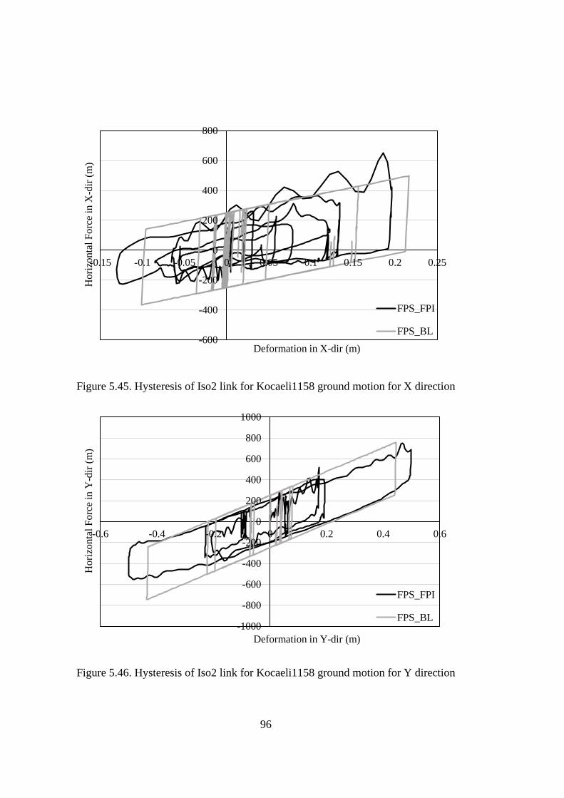
96



-600

-400

-200

0

200

400

600

800

-0.15 -0.1 -0.05 0 0.05 0.1 0.15 0.2 0.25

Ho

rizo

nta

l F

orc

e in

X-d

ir (

m)


FPS_FPI

FPS_BL

-1000

-800

-600

-400

-200

0

200

400

600

800

1000

-0.6 -0.4 -0.2 0 0.2 0.4 0.6

Ho

rizo

nta

l F

orc

e in

Y-d

ir (

m)


FPS_FPI

FPS_BL

97



-400

-300

-200

-100

0

100

200

300

-0.15 -0.1 -0.05 0 0.05 0.1 0.15 0.2 0.25

Ho

rizo

nta

l F

orc

e in

X-d

ir (

m)


FPS_FPI

FPS_BL

-1000

-800

-600

-400

-200

0

200

400

-0.6 -0.4 -0.2 0 0.2 0.4 0.6

Hori

zonta

l F

orc

e in

Y-d

ir (

m)


FPS_FPI

FPS_BL

98

5.6 Uplift Behavior

Isolators in structures with high aspect ratios are prone to tensile (uplift)

deformations during seismic actions (Feng et al., 2004; Takaoka et al., 2011; Masaki

et al., 2000) due to the overturning moment and rocking behavior. Especially

isolators that are located under the shear walls or at the corner of the building are

more susceptible to high compressive and tensile actions. In order to sustain the

stability of the isolators, the evaluation of the uplift behavior is crucial. For both

HDRB and FPS bearings, the isolator forces and deformations were obtained from

MCE seismic level with LB isolator properties. For each ground motion, peak uplift

deformations among each type were received and compared with the findings from

the literature. Also, maximum tensile forces in HDRB bearings were examined in

terms of tensile stresses.

Maximum uplift displacements of eleven ground motions are shown in Table 5.7.

For HDRB, the peak tensile displacement was retrieved as 5.07 mm from RSN316

ground motion (Westmorland, 1981) in the DHI model. This value corresponds to

2.54% tensile strain when the total rubber height of 200 mm is considered. Therefore

the HDRB design complies with the 5% tensile strain, in which isolators remain

almost linear elastic, in the Japanese literature (Kani et al., 1999; Iwabe et al., 1999;

Takayama et al., 1999) and also mentioned in Yang et al. (2010).

From Table 5.7, the maximum uplift displacement for FPS bearings was attained as

3.56 mm from the RSN850 event (Landers, 1992) among the FPS models. These

results of all cases are nearly inside the range (2-3) mm observed by Fenz (2008).

These displacement magnitudes are only instantaneous, there might be a risk of slider

topping over the isolator, which can induce severe damage. In some earthquakes,

uplift behavior for durations of 1-2 seconds were observed for the isolator under the

shear wall. Therefore, in a design project with such structural characteristics, uplift

response should be investigated carefully.

99

When BW or BL models are used instead of more comprehensive models, the uplift

displacement response can be underestimated or overestimated depending on the

ground motion.

Table 5.7 Peak uplift displacements for eleven ground motion

Uplift Displacements (mm)

HDRB-DHI HDRB-

BW HDRB-BL FPS-FPI FPS-MLP

Imperial Valley-

06_187 3.03 2.74 3.47 2.05 1.99

Westmorland_316 5.07 4.49 5.06 2.56 2.37

Chalfant

Valley_549 1.72 1.63 2.04 0.83 1.24

Chalfant Valley-

02_558 1.32 1.45 1.88 0.79 1.04

Erzican_

Turkey_821 3.74 3.32 4.12 1.67 1.60

Landers_850 2.48 2.48 2.66 3.56 3.43

Kobe_ Japan_1116 2.37 2.42 2.98 1.17 1.53

Kocaeli_

Turkey_1158 2.95 2.38 3.12 1.38 1.52

Duzce_

Turkey_1605 2.94 2.58 3.11 2.07 1.41

Chi-Chi_ Taiwan-

04_2752 2.18 2.32 2.74 1.32 1.28

Darfield_ New

Zealand_6893 1.81 1.50 2.17 1.33 1.06

For HDRB models, the maximum isolator tensile forces were obtained for each

ground motion. The forces were divided by the effective area for the corresponding

isolator type. The average response of eleven ground motion is assessed. As a result,

tensile stresses were calculated and are presented in Table 5.8. The DHI and BW

models yielded results that are close to each other and satisfying the 1 MPa tensile

limit stress, recommended by Bridgestone and Yang et al. (2010), except some

ground motions with high intensities or pulse-like behavior. However the response

of BL model showed significantly higher tensile demands on the bearings, especially

the Type 4 isolators, which are located under the shear walls due to their effective

area to bear high tensile and compressive demands.

100

Table 5.8 Peak tensile stresses for HDRB models

Maximum Tensile Stresses (kPa)

DHI Types BW Types BL Types

1 2 3 4 1 2 3 4 1 2 3 4

187 680 752 824 884 616 698 759 881 663 942 793 1084

316 1140 1274 709 1938 945 1134 780 1743 880 1155 930 1965

549 376 441 446 668 303 431 358 546 371 526 426 790

558 266 349 324 378 309 386 362 531 385 512 463 554

821 719 990 1023 1197 719 880 910 1253 825 993 1050 1597

850 484 484 619 963 490 474 618 964 521 530 640 1032

1116 419 628 482 793 482 643 437 916 521 730 525 1156

1158 659 751 882 1005 521 630 704 924 627 745 701 1210

1605 622 781 904 1036 570 685 832 950 575 844 941 916

2752 441 580 565 792 453 615 550 837 490 714 738 1061

6893 355 470 311 700 296 388 368 581 368 488 462 840

Ave 560 682 644 941 519 633 607 920 566 744 697 1110

101

CHAPTER 5

6 CONCLUSIONS

In this thesis, performance evaluation of investigated base-isolated hospital building

with irregular T plan shape and high aspect ratio (2:1) is conducted using various

nonlinear isolator models. Two types of base isolation systems, high damping rubber

bearing, and friction pendulum system, were designed according to the Turkish

Building Seismic Code (TBDY2019) using different nonlinear models. The most

commonly used types of modeling approaches in research and practice were used for

nonlinear time history analysis under eleven ground motions. For HDRB, the

deformation history integral type (DHI) model, the smoothed Bouc-Wen (BW)

bilinear model, and sharp bilinear (BL) model were considered. Moreover, the

friction and pendulum behavior (friction pendulum isolator, FPI) model and the

sharp BL model were adopted for FPS isolators. The superstructural and isolation

system response for various mathematical models are evaluated and compared in

terms of maximum isolator displacements, structural forces, floor accelerations,

inter-story drifts, and isolator uplift behavior. Based on the results, the following

conclusions can be made for the investigated building:

• The maximum isolation system displacements can be overestimated or

underestimated by the bilinear models. On average, the resulting

displacements in sharp and smoothed bilinear models are close when

compared to the highly nonlinear models for elastomeric isolators. However,

the variation in maximum displacements between the sharp bilinear (BL) and

nonlinear friction models is high. The resultant displacements are also highly

dependent on the ground motion characteristics.

• There is a significant increase in the superstructural response (superstructural

forces, floor accelerations and inter-story drifts) when idealized bilinear

models are used instead of more accurate nonlinear models. The sharp

102

transitions of BL model could result in a response that are excessively

overestimated. The smoothed bilinear model yields superstructural response

that is more acceptable and comparable with the sophisticated models.

• Among the HDRB models, the bilinear models can capture the force-

displacement behavior and energy dissipation of the rubber isolators.

However, the sharp BL model could diverge from the actual behavior when

the effect of bidirectional loading is significant. Moreover, the horizontal

stiffness of FPS isolators highly dependent on the axial load and becomes

zero during the uplift. When modeled as an FPS isolator, the sharp bilinear

model whose all three directions are uncoupled, yields unrealistic results,

especially at locations with higher overturning moments and shear walls.

• The average uplift deformations were observed to be within the safe margins

found in the literature for all HDRB and FPS models. Also, the DHI and

smooth BW model shows similar response, while the sharp BL model yielded

the highest tensile stresses and might lead to overdesign.

Although the smoothed bilinear model predicts relatively more accurate results,

both idealized bilinear models significantly overestimate the superstructural

response for this building. Many design guidelines do not include

recommendations about highly nonlinear sophisticated models. An engineer

should carefully assess the isolator models’ capabilities and possible outcoming

structural response before selecting the mathematical model to include in the

analysis and design. The results have shown that the sharp bilinear model is not

very suitable to use in the sophisticated 3-D model, especially for FPS isolators.

103

6.1 Future Studies

Although bilinear models may not capture the most realistic behavior, they are

practical to implement in the analysis software by the engineers inexperienced in the

high nonlinear concept of DHI and FPI models. The bilinear models can be modified

to capture the behavior relatively better. For HDRB isolators, the sharp BL or

smoothed BW model can be modified to include the stiffness increase when the shear

strain exceeds 200%. The modification of the BL model have been already under

investigation under a joint research by the writer, thesis supervisor and the

Bridgestone Corporation.

By experience in base-isolated hospital projects, the sharp BL model does not yield

significant superstructural response in all buildings. It is observed and studied by

several researchers in the literature and also specific for this hospital model. The

reason for this enormous difference in this thesis when compared to other isolator

models is still not very clear. The reason can be studied parametrically with different

configurations of structural and hysteretic characteristics.

105

REFERENCES

Bouc, R. (1971). Modele mathematique d’hysteresis. Acustica, 24(1), 16–25.

Calvi, P. M., & Calvi, G. M. (2018). Historical development of friction-based

seismic isolation systems. Soil Dynamics and Earthquake Engineering,

106(October 2017), 14–30. https://doi.org/10.1016/j.soildyn.2017.12.003

Chopra, A. K. (2012). Dynamics of structures : theory and applications to

earthquake engineering, 4/E.

Computers and Structures Inc. (2017). CSI Analysis Reference Manual.

Constantinou, M., Mokha, A., & Reinhorn, A. (1990). Teflon Bearings in Base

Isolation II: Modeling. Journal of Structural Engineering, 116(2), 455–474.

https://doi.org/10.1061/(ASCE)0733-9445(1990)116:2(455)

Disaster and Emergency Management Presidency, T. M. of the I. (2018). Türkiye

Bina Deprem Yönetmeliği 2019 (Vol. 30364, Issue 1).

Erdik, M., Ülker, Ö., Şadan, B., & Tüzün, C. (2018). Seismic isolation code

developments and significant applications in Turkey. Soil Dynamics and

Earthquake Engineering, 115, 413–437.

https://doi.org/10.1016/j.soildyn.2018.09.009

Erkakan, E. (2014). EXPERIMENTAL INVESTIGATION OF UPLIFT ON

SEISMIC BASE ISOLATORS. Middle East Technical University.

Feng, D., Miyama, T., Lu, X., & Ikenaga, M. (2004). A Shaking Table Test Study

on Shear Tensile Properties of Lead Rubber Bearings. 13th World Conference

on Earthquake Engineering Vancouver, B.C., Canada.

https://doi.org/10.1061/ASCEEM.1943-7889.0000007

Fenz, D. M. (2008). DEVELOPMENT, IMPLEMENTATION AND VERIFICATION

OF DYNAMIC ANALYSIS MODELS FOR MULTI-SPHERICAL SLIDING

BEARINGS. State University of New York.

Fenz, D. M., & Constantinou, M. C. (2008). Modeling Triple Friction Pendulum

Bearings for Response-History Analysis. Earthquake Spectra, 24(4), 1011–

1028. https://doi.org/10.1193/1.2982531

Furukawa, T., Ito, M., Izawa, K., & Noori, M. N. (2005). System Identification of

Base-Isolated Building using Seismic Response Data. Journal of Engineering

Mechanics, 131(3), 268–275. https://doi.org/10.1061/(ASCE)0733-

9399(2005)131:3(268)

106

Griffith, M. C., Aiken, I. D., & Kelly, J. M. (1990). Displacement Control and

Uplift Restraint for Base‐Isolated Structures. Journal of Structural

Engineering, 116(4), 1135–1148. https://doi.org/10.1061/(ASCE)0733-

9445(1990)116:4(1135)

Ibrahimbegovic, A., & Wilson, E. L. (1989). Simple numerical algorithms for the

mode superposition analysis of linear structural systems with non-proportional

damping. Computers & Structures, 33(2), 523–531.

https://doi.org/10.1016/0045-7949(89)90026-6

Kampas, G., & Makris, N. (2012). Time and frequency domain identification of

seismically isolated structures: advantages and limitations. Earthquakes and

Structures, 3(3_4), 249–270. https://doi.org/10.12989/eas.2012.3.3_4.249

Kasalanati, A., & Constantinou, M. C. (2005). Testing and Modeling of Prestressed

Isolators. Journal of Structural Engineering, 131(6), 857–866.


Kato, H., Mori, T., Murota, N., & Kikuchi, M. (2015). Analytical Model for

Elastoplastic and Creep-Like Behavior of High-Damping Rubber Bearings.

Journal of Structural Engineering, 141(9), 04014213.

https://doi.org/10.1061/(ASCE)ST.1943-541X.0001181

Kelly, J. M. (1986). Aseismic base isolation: review and bibliography. Soil

Dynamics and Earthquake Engineering, 5(4), 202–216.

https://doi.org/10.1016/0267-7261(86)90006-0

Khoshnudian, F., & Motamedi, D. (2013). Seismic response of asymmetric steel

isolated structures considering vertical component of earthquakes. KSCE

Journal of Civil Engineering, 17(6), 1333–1347.

https://doi.org/10.1007/s12205-013-0115-5

Kikuchi, M., & Aiken, I. D. (1997). An Analytical Hysteresis Model for

Elastomeric Seismic Isolation Bearings. Earthquake Engineering & Structural

Dynamics, 26(2), 215–231. https://doi.org/10.1002/(SICI)1096-

9845(199702)26:2<215::AID-EQE640>3.0.CO;2-9

Kulicki, J. M. (2014). Highway bridge design specifications. In Bridge Engineering

Handbook: Fundamentals, Second Edition (Issue September).

https://doi.org/10.1201/b15616

Makris, N., & Vassiliou, M. F. (2011). The existence of ‘complete similarities’ in

the response of seismic isolated structures subjected to pulse-like ground

motions and their implications in analysis. Earthquake Engineering &

Structural Dynamics, 40(10), 1103–1121. https://doi.org/10.1002/eqe.1072

107

Mano, T., & Mangerig, I. (2015). Determination of Tensile Capacity of

Elastomeric Bearings. Structural Engineering International, 25(2), 134–140.

https://doi.org/10.2749/101686615X14210663188376

Markou, A. A., & Manolis, G. D. (2016). Mechanical formulations for bilinear and

trilinear hysteretic models used in base isolators. Bulletin of Earthquake

Engineering, 14, 3591–3611. https://doi.org/10.1007/s10518-016-0014-5

Masaki, N., Mori, T., Murota, N., & Kasai, K. (2017). Validation of Hysteresis

Model of Deformation-History Integral Type for High Damping Rubber

Bearings. http://www.wcee.nicee.org/wcee/article/16WCEE/WCEE2017-

4583.pdf

Mavronicola, E. A. (2017). Nonlinear Modeling Considerations on the Seismic

Response of Base-Isolated Buildings: 2D and 3D Investigations of Pounding.

University of Cyprus.

Mavronicola, E., & Komodromos, P. (2014). On the response of base-isolated

buildings using bilinear models for LRBs subjected to pulse-like ground

motions: Sharp vs. smooth behaviour. Earthquake and Structures, 7(6), 1223–

1240. https://doi.org/10.12989/eas.2014.7.6.1223

Mokha, A., Constantinou, M., & Reinhorn, A. (1990). Teflon Bearings in Base

Isolation I: Testing. Journal of Structural Engineering, 116(2), 438–454.


Morgan, T. A. (2007). The Use of Innovative Base Isolation Systems to Achieve

Complex Seismic Performance Objectives. University of California, Berkeley.

Murota, N., Suzuki, S., Mori, T., Wakishima, K., Sadan, B., Tuzun, C., Sutcu, F.,

& Erdik, M. (2021). Performance of high-damping rubber bearings for seismic

isolation of residential buildings in Turkey. Soil Dynamics and Earthquake

Engineering, 143, 106620. https://doi.org/10.1016/j.soildyn.2021.106620

Naeim, F., & Kelly, J. M. (1999). Design of Seismic Isolated Structures. In

Earthquake Spectra. John Wiley & Sons, Inc.

https://doi.org/10.1002/9780470172742

Nagarajaiah, S., Reinhorn, A. M., & Constantinou, M. C. (1991). Nonlinear

Dynamic Analysis of 3‐D‐Base‐Isolated Structures. Journal of Structural

Engineering, 117(7), 2035–2054. https://doi.org/10.1061/(ASCE)0733-

9445(1991)117:7(2035)

108

Özdemir, G. (2010). RESPONSE OF ISOLATED STRUCTURES UNDER BI-

DIRECTIONAL EXCITATIONS OF NEAR-FIELD GROUND MOTIONS.

Middle East Technical University.

Park, Y. J., Wen, Y. K., & Ang, A. H.-S. (1986). Random vibration of hysteretic

systems under bi-directional ground motions. Earthquake Engineering &

Structural Dynamics, 14(4), 543–557.

https://doi.org/10.1002/eqe.4290140405

Pietra, D., & Park, A. R. L. (2017). Behaviour and Modelling of Lead-Rubber

Bearings Subjected To Tensile Actions. 16th World Conference on

Earthquake, 16WCEE.

Ray, T., Sarlis, A. A., Reinhorn, A. M., & Constantinou, M. C. (2013). Hysteretic

models for sliding bearings with varying frictional force. Earthquake

Engineering & Structural Dynamics, 42(15), 2341–2360.

https://doi.org/10.1002/eqe.2373

Robinson, W. H. (1982). Lead‐rubber hysteretic bearings suitable for protecting

structures during earthquakes. Earthquake Engineering & Structural

Dynamics, 10(4), 593–604. https://doi.org/10.1002/eqe.4290100408

Roussis, P. C. (2009). Study on the Effect of Uplift-Restraint on the Seismic

Response of Base-Isolated Structures. Journal of Structural Engineering,

135(12), 1462–1471. https://doi.org/10.1061/(ASCE)ST.1943-541X.0000070

Roussis, P. C., & Constantinou, M. C. (2006). Uplift-restraining Friction Pendulum

seismic isolation system. Earthquake Engineering & Structural Dynamics,

35(5), 577–593. https://doi.org/10.1002/eqe.545

Simo, J. C., & Hughes, T. J. R. (1997). Computational Inelasticity. Springer.

Skinner, R. I., Robinson, W. H., & McVerry, G. H. (1993). An Introduction to

Seismic Isolation. In John Wiley & Sons Ltd. https://doi.org/10.1111/j.1475-

1305.1993.tb00842.x

Subcommittee on Bridges, S. S. and T. O. (2010). Guide Specifications for Seismic

Isolation Design, AAHSTO.

Vassiliou, M. F., Tsiavos, A., & Stojadinović, B. (2013). Dynamics of inelastic

base-isolated structures subjected to analytical pulse ground motions.

Earthquake Engineering & Structural Dynamics, 056, n/a-n/a.

https://doi.org/10.1002/eqe.2311

109

Warn, G. P., & Ryan, K. L. (2012). A Review of Seismic Isolation for Buildings:

Historical Development and Research Needs. Buildings, 2, 300–325.

https://doi.org/10.3390/buildings2030300

Wen, Y.-K. (1976). Method for Random Vibration of Hysteretic Systems. Journal

of the Engineering Mechanics Division, 102(2), 249–263.

https://doi.org/10.1061/JMCEA3.0002106

Wilson, E. L. (2000). No Title. In Three Dimensional Static and Dynamic Analysis

of Structures. Computers and Structures, Inc.

http://www.edwilson.org/Book/book.htm#Author

Yakut, A., Akyüz, U., Çabuk, E., Murota, N., & Suzuki, S. (2019, July 7).

Comparison of Modeling Approaches for High Damping Rubber Bearing.

https://doi.org/10.37153/2686-7974-2019-16-902-909

Yang, Q. R., Liu, W. G., He, W. F., & Feng, D. M. (2010). Tensile Stiffness and

Deformation Model of Rubber Isolators in Tension and Tension-Shear States.

Journal of Engineering Mechanics, 136(4), 429–437.

https://doi.org/10.1061/(asce)em.1943-7889.0000007

Zayas, V. A., Low, S. S., & Mahin, S. A. (1990). A Simple Pendulum Technique

for Achieving Seismic Isolation. Earthquake Spectra, 6(2), 317–333.

https://doi.org/10.1193/1.1585573

111

APPENDICES

A. Appendix A – Time History Components of 11 Ground Motion

Figure A-1: Lateral components of Imperial Valley-06, 1979 ground motion

Figure A-2: Vertical component of Imperial Valley-06, 1979 ground motion

-0.15

-0.1

-0.05

0

0.05

0.1

0.15

0.2

0.25

0 10 20 30 40 50

Acc

(g)

Time (s)

RSN0187_225 RSN0187_315

-0.15

-0.1

-0.05

0

0.05

0.1

0.15

0.2

0 10 20 30 40 50

Acc

(g)

Time (s)

RSN0187_UP

112

Figure A-3: Lateral components of Westmorland, 1981 ground motion

Figure A-4: Vertical component of Westmorland, 1981 ground motion

-0.3

-0.25

-0.2

-0.15

-0.1

-0.05

0

0.05

0.1

0.15

0.2

0 10 20 30 40 50

Acc

(g)

Time (s)

RSN0316_225 RSN0316_315

-0.15

-0.1

-0.05

0

0.05

0.1

0.15

0.2

0 10 20 30 40 50

Acc

(g)

Time (s)

RSN0316_UP

113

Figure A-5: Lateral components of Chalfant_Valley-02_Bishop-LADWP South St,

1986 ground motion

Figure A-6: Vertical component of Chalfant_Valley-02_Bishop-LADWP South St,

1986 ground motion

-0.3

-0.25

-0.2

-0.15

-0.1

-0.05

0

0.05

0.1

0.15

0.2

0 10 20 30 40 50

Acc

(g)

Time (s)

RSN0549_180 RSN0549_270

-0.2

-0.15

-0.1

-0.05

0

0.05

0.1

0.15

0.2

0 10 20 30 40 50Acc

(g)

Time (s)

RSN0549_UP

114

Figure A-7: Lateral components of Chalfant_Valley-02_Zack Brothers Ranch St,

1986 ground motion

Figure A-8: Vertical component of Chalfant_Valley-02_Zack Brothers Ranch St,

1986 ground motion

-0.5

-0.4

-0.3

-0.2

-0.1

0

0.1

0.2

0.3

0.4

0.5

0 10 20 30 40 50Acc

(g)

Time (s)

RSN0558_270 RSN0558_360

-0.4

-0.3

-0.2

-0.1

0

0.1

0.2

0.3

0.4

0 10 20 30 40 50Acc

(g)

Time (s)

RSN0558_UP

115

Figure A-9: Lateral components of Erzincan_Turkey, 1992 ground motion

Figure A-10: Vertical component of Erzincan_Turkey, 1992 ground motion

-0.6

-0.5

-0.4

-0.3

-0.2

-0.1

0

0.1

0.2

0.3

0.4

0.5

0 5 10 15 20 25

Acc

(g)

Time (s)

RSN0821_EW RSN0821_NS

-0.2

-0.15

-0.1

-0.05

0

0.05

0.1

0.15

0.2

0.25

0.3

0 5 10 15 20 25

Acc

(g)

Time (s)

RSN0821_UP

116

Figure A-11: Lateral components of Landers, 1992 ground motion

Figure A-12: Vertical component of Landers, 1992 ground motion

-0.2

-0.15

-0.1

-0.05

0

0.05

0.1

0.15

0.2

0 10 20 30 40 50 60Acc

(g)

Time (s)

RSN0850_000 RSN0850_090

-0.2

-0.15

-0.1

-0.05

0

0.05

0.1

0.15

0 10 20 30 40 50 60

Acc

(g)

Time (s)

RSN0850_UP

117

Figure A-13: Lateral components of Kobe_Japan, 1995 ground motion

Figure A-14: Vertical component of Kobe_Japan, 1995 ground motion

-0.3

-0.25

-0.2

-0.15

-0.1

-0.05

0

0.05

0.1

0.15

0.2

0.25

0 10 20 30 40 50

Acc

(g)

Time (s)

RSN1116_000 RSN1116_090

-0.06

-0.04

-0.02

0

0.02

0.04

0.06

0.08

0 10 20 30 40 50

Acc

(g)

Time (s)

RSN1116_UP

118

Figure A-15: Lateral components of Kocaeli_Turkey, 1999 ground motion

Figure A-16: Vertical component of Kocaeli_Turkey, 1999 ground motion

-0.4

-0.3

-0.2

-0.1

0

0.1

0.2

0.3

0.4

0 5 10 15 20 25 30Acc

(g)

Time (s)

RSN1158_180 RSN1158_270

-0.25

-0.2

-0.15

-0.1

-0.05

0

0.05

0.1

0.15

0.2

0.25

0 5 10 15 20 25 30Acc

(g)

Time (s)

RSN1158_UP

119

Figure A-17: Lateral components of Duzce_Turkey, 1999 ground motion

Figure A-18: Vertical component of Duzce_Turkey, 1999 ground motion

-0.6

-0.4

-0.2

0

0.2

0.4

0.6

0 5 10 15 20 25 30Acc

(g)

Time (s)

RSN1605_180 RSN1605_270

-0.4

-0.3

-0.2

-0.1

0

0.1

0.2

0.3

0.4

0 5 10 15 20 25 30Acc

(g)

Time (s)

RSN1605_UP

120

Figure A-19: Lateral components of Chi-Chi_Taiwan-04, 1999 ground motion

Figure A-20: Vertical component of Chi-Chi_Taiwan-04, 1999 ground motion

-0.15

-0.1

-0.05

0

0.05

0.1

0.15

0.2

0 20 40 60 80 100

Acc

(g)

Time (s)

RSN2752_E RSN2752_N

-0.12

-0.1

-0.08

-0.06

-0.04

-0.02

0

0.02

0.04

0.06

0.08

0.1

0 20 40 60 80 100

Acc

(g)

Time (s)

RSN2752_V

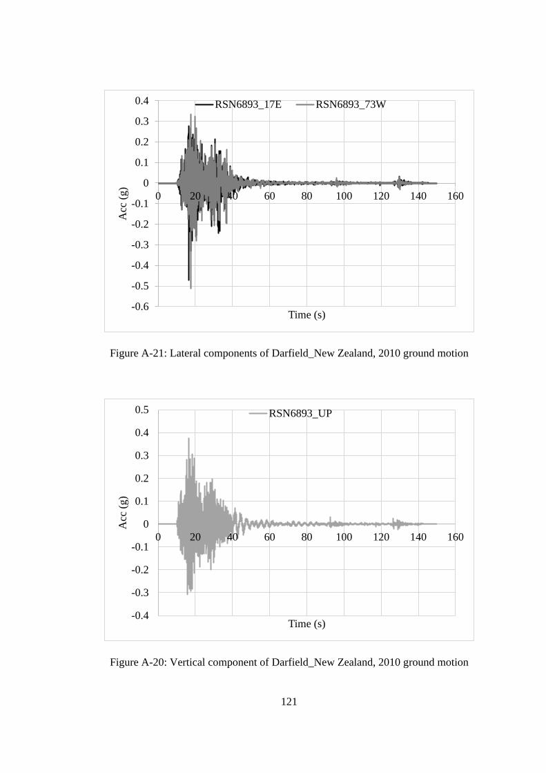
121

Figure A-21: Lateral components of Darfield_New Zealand, 2010 ground motion

Figure A-20: Vertical component of Darfield_New Zealand, 2010 ground motion

-0.6

-0.5

-0.4

-0.3

-0.2

-0.1

0

0.1

0.2

0.3

0.4

0 20 40 60 80 100 120 140 160

Acc

(g)

Time (s)

RSN6893_17E RSN6893_73W

-0.4

-0.3

-0.2

-0.1

0

0.1

0.2

0.3

0.4

0.5

0 20 40 60 80 100 120 140 160

Acc

(g)

Time (s)

RSN6893_UP

122

B. Appendix B – Comparison of Accelerations of Different Locations of the

Building

Figure B-1: Three selected joints to compare maximum accelerations

Figure B-2: Acceleration comparison of average of 7 ground motions from three

different locations and the maximum response in the X direction

-3

-2

-1

0

1

2

3

4

5

6

7

8

0 0.1 0.2 0.3 0.4 0.5

Flo

or


X-direction

1. ETABS_max

2. ETABS_joints_1

3. ETABS_joints_2

4. ETABS_joints_3

123

Figure B-2: Acceleration comparison of average of 7 ground motions from three

different locations and the maximum response in the Y direction

-3

-2

-1

0

1

2

3

4

5

6

7

8

0 0.1 0.2 0.3 0.4 0.5

Flo

or


Y-direction

1. ETABS_max

2. ETABS_joints_1

3. ETABS_joints_2

4. ETABS_joints_3

124

C. Appendix C – Hysteresis Curves Comparison for Westmorland, 1982

(RSN316) and Chalfant Valley-02 (RSN558) Ground Motions

Figure C-1: The selected isolator locations to compare hysteretic response (the


• HDRB Comparison

Figure C-2: Axial load history of selected isolators for RSN316 ground motion

-12000

-10000

-8000

-6000

-4000

-2000

0

2000

0 5 10 15 20 25 30 35 40 45

Axia

l F

orc

e (k

N)

Time (s)

Axial Force History @ Westmorland316

Iso1

Iso2

Iso3

125

Figure C-3: Hysteresis of Iso1 models under RSN316 ground motion in X dir.

Figure C-4: Hysteresis of Iso1 models under RSN316 ground motion in Y dir.

-800

-600

-400

-200

0

200

400

600

800

-0.4 -0.3 -0.2 -0.1 0 0.1 0.2 0.3 0.4

Ho

rizo

nta

l F

orc

e in

X-d

ir (

m)


HDRB_DHI

HDRB_BW

HDRB_BL

-800

-600

-400

-200

0

200

400

600

800

1000

-0.6 -0.4 -0.2 0 0.2 0.4 0.6 0.8

Hori

zon

tal

Forc

e in

Y-d

ir (

m)


HDRB_DHI

HDRB_BW

HDRB_BL

126



-800

-600

-400

-200

0

200

400

600

800

-0.4 -0.3 -0.2 -0.1 0 0.1 0.2 0.3 0.4

Ho

rizo

nta

l F

orc

e in

X-d

ir (

m)


HDRB_DHI

HDRB_BW

HDRB_BL

-800

-600

-400

-200

0

200

400

600

800

1000

-0.6 -0.4 -0.2 0 0.2 0.4 0.6 0.8

Hori

zonta

l F

orc

e in

Y-d

ir (

m)


HDRB_DHI

HDRB_BW

HDRB_BL

127



-600

-400

-200

0

200

400

600

-0.4 -0.3 -0.2 -0.1 0 0.1 0.2 0.3 0.4

Ho

rizo

nta

l F

orc

e in

X-d

ir (

m)


HDRB_DHI

HDRB_BW

HDRB_BL

-800

-600

-400

-200

0

200

400

600

800

1000

-0.5 -0.3 -0.1 0.1 0.3 0.5 0.7 0.9

Hori

zon

tal

Forc

e in

Y-d

ir (

m)


HDRB_DHI

HDRB_BW

HDRB_BL

128



-12000

-10000

-8000

-6000

-4000

-2000

0

2000

0 5 10 15 20 25 30 35 40 45

Axia

l F

orc

e (k

N)

Time (s)

Axial Force History @ Chalfant Valley558

Iso1

Iso2

Iso3

-500

-400

-300

-200

-100

0

100

200

300

400

500

-0.25 -0.2 -0.15 -0.1 -0.05 0 0.05 0.1 0.15 0.2

Hori

zonta

l F

orc

e in

X-d

ir (

m)


HDRB_DHI

HDRB_BW

HDRB_BL

129


-400

-300

-200

-100

0

100

200

300

400

-0.15 -0.1 -0.05 0 0.05 0.1 0.15

Ho

rizo

nta

l F

orc

e in

Y-d

ir (

m)


HDRB_DHI

HDRB_BW

HDRB_BL

130



-500

-400

-300

-200

-100

0

100

200

300

400

-0.25 -0.2 -0.15 -0.1 -0.05 0 0.05 0.1 0.15 0.2

Ho

rizo

nta

l F

orc

e in

X-d

ir (

m)


HDRB_DHI

HDRB_BW

HDRB_BL

-400

-300

-200

-100

0

100

200

300

400

-0.15 -0.1 -0.05 0 0.05 0.1 0.15

Hori

zonta

l F

orc

e in

Y-d

ir (

m)


HDRB_DHI

HDRB_BW

HDRB_BL

131



-400

-300

-200

-100

0

100

200

300

400

-0.25 -0.2 -0.15 -0.1 -0.05 0 0.05 0.1 0.15 0.2

Ho

rizo

nta

l F

orc

e in

X-d

ir (

m)


HDRB_DHI

HDRB_BW

HDRB_BL

-300

-200

-100

0

100

200

300

-0.15 -0.1 -0.05 0 0.05 0.1 0.15

Hori

zon

tal

Forc

e in

Y-d

ir (

m)


HDRB_DHI

HDRB_BW

HDRB_BL

132

• FPS Comparison



-12000

-10000

-8000

-6000

-4000

-2000

0

2000

0 5 10 15 20 25 30 35 40 45

Axia

l F

orc

e (k

N)

Time (s)

Axial Force History @ Westmorland316

Iso1

Iso2

Iso3

-800

-600

-400

-200

0

200

400

600

800

1000

-0.4 -0.3 -0.2 -0.1 0 0.1 0.2 0.3 0.4

Hori

zonta

l F

orc

e in

X-d

ir (

m)


FPS_FPI

FPS_BL

133


-1000

-500

0

500

1000

1500

-0.6 -0.4 -0.2 0 0.2 0.4 0.6 0.8 1

Ho

rizo

nta

l F

orc

e in

Y-d

ir (

m)


FPS_FPI

FPS_BL

134



-600

-400

-200

0

200

400

600

800

1000

-0.4 -0.3 -0.2 -0.1 0 0.1 0.2 0.3 0.4

Ho

rizo

nta

l F

orc

e in

X-d

ir (

m)


FPS_FPI

FPS_BL

-1000

-500

0

500

1000

1500

-0.6 -0.4 -0.2 0 0.2 0.4 0.6 0.8 1

Hori

zonta

l F

orc

e in

Y-d

ir (

m)


FPS_FPI

FPS_BL

135



-200

-100

0

100

200

300

400

500

600

-0.4 -0.3 -0.2 -0.1 0 0.1 0.2 0.3 0.4

Ho

rizo

nta

l F

orc

e in

X-d

ir (

m)


FPS_FPI

FPS_BL

-1000

-800

-600

-400

-200

0

200

400

600

-0.6 -0.4 -0.2 0 0.2 0.4 0.6 0.8 1

Hori

zonta

l F

orc

e in

Y-d

ir (

m)


FPS_FPI

FPS_BL

136



-12000

-10000

-8000

-6000

-4000

-2000

0

2000

0 5 10 15 20 25 30 35 40 45

Axia

l F

orc

e (k

N)

Time (s)

Axial Force History @ Chalfant Valley558

Iso1

Iso2

Iso3

-800

-600

-400

-200

0

200

400

600

-0.2 -0.15 -0.1 -0.05 0 0.05 0.1 0.15 0.2

Hori

zonta

l F

orc

e in

X-d

ir (

m)


FPS_FPI

FPS_BL

137


-500

-400

-300

-200

-100

0

100

200

300

400

500

-0.15 -0.1 -0.05 0 0.05 0.1 0.15

Ho

rizo

nta

l F

orc

e in

Y-d

ir (

m)


FPS_FPI

FPS_BL

138



-600

-400

-200

0

200

400

600

800

-0.2 -0.15 -0.1 -0.05 0 0.05 0.1 0.15 0.2

Ho

rizo

nta

l F

orc

e in

X-d

ir (

m)


FPS_FPI

FPS_BL

-400

-300

-200

-100

0

100

200

300

400

500

-0.15 -0.1 -0.05 0 0.05 0.1 0.15

Hori

zonta

l F

orc

e in

Y-d

ir (

m)


FPS_FPI

FPS_BL

139



-300

-250

-200

-150

-100

-50

0

50

100

150

200

-0.2 -0.15 -0.1 -0.05 0 0.05 0.1 0.15 0.2

Ho

rizo

nta

l F

orc

e in

X-d

ir (

m)


FPS_FPI

FPS_BL

-250

-200

-150

-100

-50

0

50

100

150

200

-0.15 -0.1 -0.05 0 0.05 0.1 0.15

Hori

zonta

l F

orc

e in

Y-d

ir (

m)


FPS_FPI

FPS_BL

140

D. Appendix D – Performance Comparison for 5% and 2% superstructural

damping

Figure D-1: Average floor accelerations for HDRB models in X direction

Figure D-2: Average floor accelerations for HDRB models in Y direction

-10

0

10

20

30

40

50

0 0.1 0.2 0.3 0.4

Flo

or

Hei

gh

t (m

)



HDRB_DHI_%5 HDRB_DHI_%2

-10

0

10

20

30

40

50

0 0.1 0.2 0.3 0.4

Flo

or

Hei

gh

t (m

)




141

Figure D-3: Average floor accelerations for FPS models in X direction

Figure D-4: Average floor accelerations for FPS models in Y direction

-10

0

10

20

30

40

50

0 0.1 0.2 0.3 0.4 0.5 0.6

Flo

or

Hei

gh

t (m

)



FPS_FPI_%5 FPS_FPI_%2

-10

0

10

20

30

40

50

0 0.2 0.4 0.6 0.8

Flo

or

Hei

gh

t (m

)




142

Figure D-5: Average interstory drifts for HDRB models in X direction

Figure D-6: Average interstory drifts for HDRB models in Y direction

0

5

10

15

20

25

30

35

40

45

0 0.002 0.004 0.006 0.008 0.01

Flo

or

Hei

gh

t (m

)

Story Drift



0

5

10

15

20

25

30

35

40

45

0 0.002 0.004 0.006 0.008 0.01

Flo

or

Hei

gh

t (m

)

Story Drift



143

Figure D-7: Average interstory drifts for FPS models in X direction

Figure D-8: Average interstory drifts for FPS models in Y direction

0

5

10

15

20

25

30

35

40

45

0 0.002 0.004 0.006 0.008 0.01

Flo

or

Hei

gh

t (m

)

Story Drift



0

5

10

15

20

25

30

35

40

45

0 0.002 0.004 0.006 0.008 0.01

Flo

or

Hei

gh

t (m

)

Story Drift



144

E. Appendix E – Performance Comparison for FNA and DI methods

Figure E-1: Hysteresis curves for Iso3 under Kocaeli1158 ground motion in X dir

Figure E-2: Hysteresis curves for Iso3 under Kocaeli1158 ground motion in Y dir

-600

-400

-200

0

200

400

600

-0.6 -0.4 -0.2 0 0.2 0.4 0.6

Shea

r F

orc

e (k

N)

Shear Deformation (m)

X-Dir-HDRI-MCE-LB

DI

FNA

-300

-200

-100

0

100

200

300

-0.2 -0.15 -0.1 -0.05 0 0.05 0.1 0.15 0.2

Shea

r F

orc

e (k

N)

Shear Deformation (m)

Y-Dir-HDRI-MCE-LB

DI

FNA

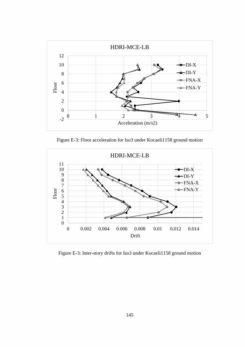
145

Figure E-3: Floor acceleration for Iso3 under Kocaeli1158 ground motion

Figure E-3: Inter-story drifts for Iso3 under Kocaeli1158 ground motion

-2

0

2

4

6

8

10

12

0 1 2 3 4 5

Flo

or

Acceleration (m/s2)

HDRI-MCE-LB

DI-X

DI-Y

FNA-X

FNA-Y

0123456789

1011

0 0.002 0.004 0.006 0.008 0.01 0.012 0.014

Flo

or

Drift

HDRI-MCE-LB

DI-X

DI-Y

FNA-X

FNA-Y

146

Figure E-5: Hysteresis curves for Iso3 under Duzce1605 ground motion in X dir

Figure E-6: Hysteresis curves for Iso3 under Duzce1605 ground motion in Y dir

-300

-200

-100

0

100

200

300

400

500

-0.1 -0.05 0 0.05 0.1 0.15 0.2Shea

r F

orc

e (k

N)

Shear Displacement (m)

X-Dir-MLP-DBE-Nom

DI

FNA

-300

-200

-100

0

100

200

300

-0.1 -0.05 0 0.05 0.1

Shea

r F

orc

e (k

N)

Shear Displacement (m)

Y-Dir-MLP-DBE-Nom

DI

FNA

147

Figure E-7: Floor accelerations for Iso3 under Duzce1605 ground motion

Figure E-8: Inter-story drifts for Iso3 under Duzce1605 ground motion

-2

0

2

4

6

8

10

12

0 1 2 3 4 5 6

Flo

or

Acceleration (m/s2)

MLP-DBE-Nom

DI-X

DI-Y

FNA-X

FNA-Y

0

2

4

6

8

10

12

0 0.002 0.004 0.006 0.008 0.01

Flo

or

Drift

MLP-DBE-Nom

DI-X

DI-Y

FNA-X

FNA-Y

seismic performance comparison of base-isolated …

Documents