seismic performance assessment of buildings
TRANSCRIPT
8/12/2019 Seismic Performance Assessment of Buildings
http://slidepdf.com/reader/full/seismic-performance-assessment-of-buildings 1/358
FEMA P-58/ Pre-Release August 2012
Seismic Performance Assessment of Buildings
Volume 2 – Implementation Guide
Prepared by
APPLIED TECHNOLOGY COUNCIL201 Redwood Shores Parkway, Suite 240
Redwood City, California 94065www.ATCouncil.org
Prepared for
FEDERAL EMERGENCY MANAGEMENT AGENCYMichael Mahoney, Project Officer
Robert D. Hanson, Technical MonitorWashington, D.C.
ATC MANAGEMENT AND OVERSIGHT
Christopher Rojahn (Project Executive Director)Jon A. Heintz (Project Manager)Ayse Hortacsu
PROJECT MANAGEMENT COMMITTEERonald O. Hamburger (Project Technical Director)John GillengertenWilliam T. Holmes **Peter J. MayJack P. MoehleMaryann T. Phipps*
STEERING COMMITTEE
William T. Holmes (Chair)Roger D. BorcherdtAnne BostromBruce BurrKelly CobeenAnthony B. CourtTerry DooleyDan GramerMichael GriffinR. Jay LoveDavid MarSteven McCabeBrian J. Meacham
William J. Petak
* ATC Board Contact** ex-officio
RISK MANAGEMENT PRODUCTS TEAM
John D. Hooper (Co-Team Leader)Craig D. Comartin (Co-Team Leader)Mary ComerioAllin CornellMahmoud HachemGee HecksherJudith Mitrani-ReiserPeter MorrisFarzad NaeimKeith PorterHope Seligson
STRUCTURAL PERFORMANCE
PRODUCTS TEAMAndrew S. Whittaker (Team Leader)Gregory DeierleinJohn D. HooperYin-Nan HuangLaura Lowes Nicolas LucoAndrew T. Merovich
NONSTRUCTURAL PERFORMANCEPRODUCTS TEAM
Robert E. Bachman (Team Leader)Philip J. Caldwell
Andre FiliatraultRobert P. KennedyHelmut KrawinklerManos MaragakisGilberto MosquedaEduardo MirandaKeith Porter

8/12/2019 Seismic Performance Assessment of Buildings
http://slidepdf.com/reader/full/seismic-performance-assessment-of-buildings 2/358
RISK MANAGEMENT PRODUCTSCONSULTANTS
Travis ChrupaloD. Jared DeBockArmen Der KiureghianScott Hagie
Curt HaseltonRussell LarsenJuan Murcia-DelsoScott ShellP. Benson ShingFarzin Zareian
STRUCTURAL PERFORMANCEPRODUCTS AND FRAGILITYDEVELOPMENT CONSULTANTS
Jack BakerDhiman BasuDan Dolan
Charles EkiertAndre FiliatraultAysegul GogusKerem GulecDawn LehmanJingjuan LiEric LumpkinJuan Murcia-DelsoHussein OkailCharles RoederP. Benson ShingChristopher SmithVictor Victorsson
John Wallace
NONSTRUCTURAL PERFORMANCEPRODUCTS AND FRAGILITYDEVELOPMENT CONSULTANTS
Richard BehrGreg HardyChristopher Higgins
Gayle JohnsonPaul KremerDave McCormickAli M. MemariWilliam O’BrienJohn OsteraasElizabeth PahlJohn StevensonXin Xu
FRAGILITY REVIEW PANELBruce EllingwoodRobert P. Kennedy
Stephen MahinVALIDATION/VERIFICATION TEAMCharles Scawthorn (Chair)Jack BakerDavid BonnevilleHope Seligson
SPECIAL REVIEWERSThalia AnagnosFouad M. Bendimerad
Notice
Any opinions, findings, conclusions, or recommendations expressed in this publication do not
necessarily reflect the views of the Applied Technology Council (ATC), the Department of
Homeland Security (DHS), or the Federal Emergency Management Agency (FEMA).
Additionally, neither ATC, DHS, FEMA, nor any of their employees, makes any warranty,expressed or implied, nor assumes any legal liability or responsibility for the accuracy,
completeness, or usefulness of any information, product, or process included in this publication.
Users of information from this publication assume all liability arising from such use.
Cover photograph – Collapsed building viewed through the archway of an adjacent building, 1999 Chi-Chi,Taiwan earthquake (courtesy of Farzad Naeim, John A. Martin & Associates, Los Angeles, California).
8/12/2019 Seismic Performance Assessment of Buildings
http://slidepdf.com/reader/full/seismic-performance-assessment-of-buildings 3/358
Pre-Release Version August 2012
FEMA P-58 – Vol. 2 Preface iii
Preface
In 2001, the Applied Technology Council (ATC) was awarded the first in a
series of contracts with the Federal Emergency Management Agency
(FEMA) to develop Next-Generation Performance-Based Seismic Design
Guidelines for New and Existing Buildings. These projects would become
known as the ATC-58/ATC-58-1 Projects. The principal product under this
combined 10-year work effort was the development of a methodology for
seismic performance assessment of individual buildings that properly
accounts for uncertainty our ability to accurately predict response, and
communicates performance in ways that better relate to the decision-making
needs of stakeholders.
This report, Seismic Performance Assessment of Buildings, Volume 2 –
Implementation Guide, is one in a series of products that together describe
the resulting methodology and its implementation. The procedures are
probabilistic, uncertainties are explicitly considered, and performance is
expressed as the probable consequences, in terms of human losses (deaths
and serious injuries), direct economic losses (building repair or replacement
costs), and indirect losses (repair time and unsafe placarding) resulting from
building damage due to earthquake shaking. The methodology is general
enough to be applied to any building type, regardless of age, construction or
occupancy; however, basic data on structural and nonstructural
damageability and consequence are necessary for its implementation.
To allow for practical implementation of the methodology, work included the
collection of fragility and consequence data for most common structural
systems and building occupancies, and the development of an electronic
Performance Assessment Calculation Tool (PACT) for performing the
probabilistic computations and accumulation of losses. The purpose of this
Volume 2 –Implementation Guide is to provide users with step-by-step
guidance in the development of basic building information, response
quantities, fragilities, and consequence data used as inputs to themethodology.
This work is the result of more than 130 consultants involved in the
development of the methodology and underlying procedures, collection of
available fragility data, estimation of consequences, development of
supporting electronic tools, implementation of quality assurance procedures,
and beta testing efforts. ATC is particularly indebted to the leadership of
8/12/2019 Seismic Performance Assessment of Buildings
http://slidepdf.com/reader/full/seismic-performance-assessment-of-buildings 4/358
August 2012 Pre-Release Version
iv Preface FEMA P-58 – Vol. 2
Ron Hamburger, who served as Project Technical Director, John Hooper and
Craig Comartin, who served as Risk Management Products Team Leaders,
Andrew Whittaker, who served as Structural Performance Products Team
Leader, Bob Bachman, who served as Nonstructural Performance Products
Team Leader, and the members of the Project Management Committee,
including John Gillengerten, Bill Holmes, Peter May, Jack Moehle, and
Maryann Phipps. ATC is also indebted to Andy Merovich, Structural
Performance Products Team Member, for his lead role in the development of
this volume.
ATC would also like to thank the members of the Project Steering
Committee, the Risk Management Products Team, the Structural
Performance Products Team, the Nonstructural Performance Products Team,
the Fragility Review Panel, the Validation/Verification Team, and the many
consultants who assisted these teams. The names of individuals who served
on these groups, along with their affiliations, are provided in the list of
Project Participants at the end of this report.
ATC acknowledges the Pacific Earthquake Engineering Research Center
(PEER), and its framework for performance-based earthquake engineering,
as the technical basis underlying the methodology. In particular, the work of
Tony Yang, Jack Moehle, Craig Comartin, and Armen Der Kiureghian, in
developing and presenting the first practical application of the PEER
framework, is recognized as the basis of how computations are performed
and losses are accumulated in the methodology.
Special acknowledgment is extended to C. Allin Cornell and Helmut
Krawinkler for their formative work in contributing to risk assessment and
performance-based design methodologies, and to whom this work is
dedicated.
ATC also gratefully acknowledges Michael Mahoney (FEMA Project
Officer) and Robert Hanson (FEMA Technical Monitor) for their input and
guidance in the conduct of this work, and Peter N. Mork, Bernadette
Hadnagy, and Laura Samant for ATC report production services.
Jon A. Heintz Christopher RojahnATC Director of Projects ATC Executive Director
8/12/2019 Seismic Performance Assessment of Buildings
http://slidepdf.com/reader/full/seismic-performance-assessment-of-buildings 5/358
Pre-Release Version August 2012
FEMA-P-58 – Vol. 2 Table of Contents v
Table of Contents
Preface ........................................................................................................... iii
List of Figures ............................................................................................... xi
List of Tables .............................................................................................. xix
1. Introduction ...................................................................................... 1-1
1.1 Purpose ..................................................................................... 1-1
1.2 Scope ........................................................................................ 1-1
1.3 Limitations ............................................................................... 1-2
1.4 The Basic Steps ........................................................................ 1-2
1.5 Assessment Types .................................................................... 1-3
1.6 Performance Measures ............................................................. 1-41.7 Analysis Methods ..................................................................... 1-4
1.8 Document Organization ........................................................... 1-5
2 Building Performance Modeling ..................................................... 2-1
2.1 Introduction .............................................................................. 2-1
2.2 Building Characteristics ........................................................... 2-12.2.1 Project Information ..................................................... 2-12.2.2 Building Information ................................................... 2-22.2.3 Population Model ........................................................ 2-8
2.3 Fragility Specifications and Performance Groups .................. 2-10
2.4 Identification of Vulnerable Structural Components and
Systems ................................................................................... 2-15
2.4.1 Structural Steel Elements (B103) .............................. 2-16
2.4.2 Reinforced Concrete Elements (B104) ...................... 2-18
2.4.3 Reinforced Masonry Elements (B105) ...................... 2-22
2.4.4 Cold-Formed Steel Structural Elements (B106) ........ 2-23
2.4.5 Wood Light Frame Structural Elements (B107) ....... 2-242.4.6 Structural Performance Groups ................................. 2-24
2.5 Identification of Vulnerable Nonstructural Components
and Systems ............................................................................ 2-262.5.1 Exterior Nonstructural Walls (B201) ........................ 2-292.5.2 Exterior Windows (B202) ......................................... 2-312.5.3 Roof Elements (B30) ................................................. 2-322.5.4 Partitions (C101) ....................................................... 2-33
2.5.5 Stairs (C201) ............................................................. 2-342.5.6 Wall Finishes (C301)................................................. 2-352.5.7 Floor Finishes, Raised Access Floors, Floor Flooding
(C302)........................................................................ 2-362.5.8 Suspended Ceilings and Ceiling Lighting (C303) ..... 2-362.5.9 Elevators and Lifts (D101) ........................................ 2-382.5.10 Domestic Hot and Cold Water Piping (D202) .......... 2-382.5.11 Sanitary Waste Piping (D203) ................................... 2-392.5.12 Chilled Water and Steam Piping (D205 and D206) .. 2-39
8/12/2019 Seismic Performance Assessment of Buildings
http://slidepdf.com/reader/full/seismic-performance-assessment-of-buildings 6/358
August 2012 Pre-Release Version
vi Table of Contents FEMA-P-58 – Vol. 2
2.5.13 Chillers, Cooling Towers, Compressors (D303) ....... 2-402.5.14 HVAC Distribution Systems (D304) ......................... 2-412.5.15 Control Panels (D305) ............................................... 2-422.5.16 Packaged Air Handling Units (D306) ........................ 2-422.5.17 Fire Protection (D401) ............................................... 2-432.5.18 Motor Control Centers, Transformers, LV Switchgear,
Distribution Panels (D501) ........................................ 2-442.5.19 Other Electrical Systems (D509) ............................... 2-452.5.20 Equipment and Furnishings (E20) ............................. 2-462.5.21 Special Construction (F20) ........................................ 2-47
2.6 Collapse Fragility Analysis ..................................................... 2-472.6.1 Nonlinear Response-History Analysis Approach ...... 2-482.6.2 Nonlinear Static Analysis Approach ......................... 2-482.6.3 Judgment-Based Approach ........................................ 2-532.6.4 Collapse Modes and PACT Input .............................. 2-54
2.7 Residual Drift Fragility ........................................................... 2-55
3. Performing Assessments .................................................................. 3-1
3.1 Introduction............................................................................... 3-1
3.2 Building Analytical Model ....................................................... 3-13.2.1 Nonlinear Response-History Analysis ......................... 3-23.2.2 Simplified Analysis ..................................................... 3-33.2.3 Demand Directionality ................................................. 3-4
3.3 Intensity-Based Assessment ..................................................... 3-43.3.1 Nonlinear Response-History Analysis ......................... 3-43.3.2 Simplified Analysis ................................................... 3-103.3.3 Review Results .......................................................... 3-28
3.4 Scenario-Based Assessment ................................................... 3-343.4.1 Response History Analysis ........................................ 3-353.4.2 Simplified Analysis ................................................... 3-403.4.3 Review Results .......................................................... 3-44
3.5 Time-Based Assessment ......................................................... 3-443.5.1 Nonlinear Response-History Analysis ....................... 3-443.5.2 Simplified Analysis ................................................... 3-463.5.3 Review Results .......................................................... 3-53
4. Example Application: Intensity-Based Assessment UsingSimplified Analysis ........................................................................... 4-1
4.1 Introduction............................................................................... 4-1
4.2 Obtain Site and Building Description ....................................... 4-1
4.3 Select Assessment Type and Performance Measure ................. 4-3
4.4 Assemble Building Performance Model ................................... 4-34.4.1 Project Information ...................................................... 4-34.4.2 Building Information ................................................... 4-4
4.4.3 Population Distribution ................................................ 4-54.4.4 Fragility Specifications and Performance Groups ....... 4-54.4.5 Collapse Fragility and Collapse Modes ..................... 4-204.4.6 Residual Drift Fragility .............................................. 4-23
4.5 Select Analysis Method and Construct Building Analytical
Model ...................................................................................... 4-23
4.6 Define Earthquake Hazards .................................................... 4-244.7 Analyze Building Response .................................................... 4-27
4.7.1 Estimate Median Peak Story Drift and Dispersion .... 4-27
8/12/2019 Seismic Performance Assessment of Buildings
http://slidepdf.com/reader/full/seismic-performance-assessment-of-buildings 7/358
Pre-Release Version August 2012
FEMA-P-58 – Vol. 2 Table of Contents vii
4.7.2 Estimate Median Peak Floor Acceleration andDispersion .................................................................. 4-29
4.7.3 Estimate Median Residual Story Drift andDispersion .................................................................. 4-30
4.8 Input Response Data and Calculate Performance................... 4-31
4.9 Review Results for Selected Performance Measures ............. 4-34
4.10 Summary and Discussion ....................................................... 4-34
5. Example Application: Time-Based Assessment UsingNonlinear Response-History Analysis ............................................ 5-1
5.1 Introduction .............................................................................. 5-1
5.2 Obtain Site and Building Description....................................... 5-1
5.3 Select Assessment Type and Performance Measures ............... 5-2
5.4 Assemble Performance Assessment Model .............................. 5-4
5.5 Select Analysis Method and Construct Building Analytical
Model ....................................................................................... 5-35.6 Define Earthquake Hazards ...................................................... 5-3
5.7 Analyze Building Response ................................................... 5-11
5.8 Input Response Data and Calculate Performance................... 5-155.9 Review Results for Selected Performance Measures ............. 5-17
6. Structural Fragility Calculation ..................................................... 6-1
6.1 Introduction .............................................................................. 6-1
6.2 Building Description ................................................................ 6-1
6.3 Development of Structural Components and System Fragilities
by Calculation .......................................................................... 6-56.3.1 Plywood Roof Diaphragm ........................................... 6-56.3.2 Tilt-Up Walls ............................................................. 6-136.3.3 Wall/Roof Attachments ............................................. 6-20
6.4 PACT Modifications .............................................................. 6-30
7. Nonstructural Fragility Calculation ............................................... 7-17.1 Introduction .............................................................................. 7-17.2 Unanchored Components ......................................................... 7-1
7.2.1 Overturning ................................................................. 7-27.2.2 Sliding ......................................................................... 7-6
7.3 Anchored Components ............................................................. 7-77.3.1 Code Based Limit State Determination of
Anchorage Fragility ..................................................... 7-77.3.2 Strength-Based Limit State Approach to Anchorage
Fragility Calculation .................................................. 7-13
7.4 Displacement Based Limit State Approach to Define
Calculated Fragilities .............................................................. 7-16
8. User-Defined Consequence Functions ............................................ 8-1
8.1 Introduction .............................................................................. 8-1
8.2 General Considerations ............................................................ 8-1
8.3 Performance Measure Consequences ....................................... 8-38.3.1 Repair Cost .................................................................. 8-38.3.2 Repair Time ................................................................. 8-58.3.3 Unsafe Placards ........................................................... 8-68.3.4 Casualties .................................................................... 8-8
8/12/2019 Seismic Performance Assessment of Buildings
http://slidepdf.com/reader/full/seismic-performance-assessment-of-buildings 8/358
August 2012 Pre-Release Version
viii Table of Contents FEMA-P-58 – Vol. 2
8.4 Database Modifications ............................................................ 8-98.4.1 New Consequence Function ........................................ 8-9
8.5 Example Application .............................................................. 8-128.5.1 Establish Baseline Repair Cost .................................. 8-128.5.2 Establish Cost Ranges................................................ 8-148.5.3 Establish Time Estimates ........................................... 8-14
8.6 Other Considerations .............................................................. 8-148.6.1 Time and Location Adjustments ................................ 8-148.6.2 Double Counting ........................................................ 8-15
Appendix A: Structural Component and System FragilitySpecifications ................................................................................... A-1
Appendix B: Nonstructural Component and System Fragilities .......... B-1
B-1 B20: Exterior Enclosure (Tables B201, B202) ........................ B-1
B-2 C10: Interior Construction (Table C101) ................................. B-7
B-3 C20: Stairs (Table C201) ......................................................... B-7
B-4 C30: Interior Finishes (Tables C301, C302) ............................ B-8
B-5 D20: Plumbing and Piping (Tables D202, D203, D205,
D206) ..................................................................................... B-10
B-6 D30: HVAC (Tables D303, D304, D305, D306) .................. B-12
B-7 D50: Electrical (Tables D501 and D509) .............................. B-18
Appendix C: PACT User’s Manual ......................................................... C-1
C.1 Introduction.............................................................................. C-1
C.2 Hardware and Software Requirements .................................... C-1
C.3 Installing PACT ....................................................................... C-1
C.4 What is new in PACT? ............................................................ C-2C.4.1 General ........................................................................ C-2C.4.2 Fragilities .................................................................... C-3C.4.3 Building Manager ....................................................... C-3
C.4.4 Engine ......................................................................... C-4C.4.5 Viewing Results .......................................................... C-4
C.5 Using PACT............................................................................. C-4C.5.1 PACT Control Panel ................................................... C-4C.5.2 Model the Building and Import Analyses Results ...... C-5C.5.3 Performance Evaluation ............................................ C-18C.5.4 Evaluating Results .................................................... C-21
C.6 PACT Utilities ....................................................................... C-37C.6.1 Fragility Manager ..................................................... C-37C.6.2 Population Manager .................................................. C-51C.6.3 Reporting .................................................................. C-52
C.7 A Look under the Hood ......................................................... C-53
C.7.1 Project Files .............................................................. C-54C.7.2 Results Files .............................................................. C-54C.7.3 Fragility Specification Files ...................................... C-54C.7.4 Population Specification Files .................................. C-55C.7.5 Reporting Template Files ......................................... C-55C.7.5 Programming Notes .................................................. C-55
Appendix D: Normative Quantity Estimation Tool ............................... D-1
D.1 Introduction.............................................................................. D-1

8/12/2019 Seismic Performance Assessment of Buildings
http://slidepdf.com/reader/full/seismic-performance-assessment-of-buildings 9/358

8/12/2019 Seismic Performance Assessment of Buildings
http://slidepdf.com/reader/full/seismic-performance-assessment-of-buildings 10/358

8/12/2019 Seismic Performance Assessment of Buildings
http://slidepdf.com/reader/full/seismic-performance-assessment-of-buildings 11/358
Pre-Release Version August 2012
FEMA P-58 – Vol. 2 List of Figures xi
List of Figures
Figure 1-1 Performance assessment process ....................................... 1-3
Figure 2-1 Format of PACT screenshots used, indicating the tab
title location ...................................................................... 2-1
Figure 2-2 PACT Project Information tab ........................................... 2-2
Figure 2-3 PACT Building Information tab ........................................ 2-3
Figure 2-4 Definition of floor and story numbers and floor and
story heights ....................................................................... 2-4
Figure 2-5 PACT Population tab showing commercial office
occupancy .......................................................................... 2-9
Figure 2-6 PACT Population Manager utility ................................... 2-10
Figure 2-7 PACT Fragilities tab showing fragility specification
selection ........................................................................... 2-12
Figure 2-8 PACT Performance Groups tab. ...................................... 2-26
Figure 2-9 Normative Quantity Estimation tool Building Definition
table. ................................................................................. 2-28
Figure 2-10 Normative Quantity Estimation tool Component
Summary Matrix. ............................................................. 2-29
Figure 2-11 SPO2IDA idealized pushover curve for hypothetical
structure ........................................................................... 2-49
Figure 2-12 Plan of example structure................................................. 2-50
Figure 2-13 Section of example structure ............................................ 2-50
Figure 2-14 Pushover curve for 2-story CMU building. ..................... 2-51
Figure 2-15 SPO2IDA Input ............................................................... 2-52
Figure 2-16 SPO2IDA Output ............................................................. 2-52
Figure 2-17 Comparison of collapse fragility functions obtained with two
different approaches: SPO2IDA and Judgment. .............. 2-54
Figure 2-18 Illustration of multiple collapse modes ............................ 2-55

8/12/2019 Seismic Performance Assessment of Buildings
http://slidepdf.com/reader/full/seismic-performance-assessment-of-buildings 12/358
August 2012 Pre-Release Version
xii List of Figures FEMA P-58 – Vol. 2
Figure 2-19 PACT Residual Drift tab .................................................. 2-56
Figure 3-1 Performance assessment procedure showing steps
covered in this chapter in shaded box. ............................... 3-1
Figure 3-2 Example spectra for scaled suite of 5 motions ................... 3-6
Figure 3-3 PACT Structural Analysis Results tab with response
history drift input .............................................................. 3-10
Figure 3-4 PACT Residual Drift input. .............................................. 3-10
Figure 3-5 Lumped weight distribution ............................................. 3-15
Figure 3-6 Results from linear analysis ............................................. 3-15
Figure 3-7 PACT Structural Analysis Results tab ............................. 3-25
Figure 3-8 PACT Residual Drift tab .................................................. 3-28
Figure 3-9 PACT Control Panel ........................................................ 3-28
Figure 3-10 PACT Engine window ..................................................... 3-29
Figure 3-11 PACT Cost tab ................................................................. 3-30
Figure 3-12 PACT Repair Time tab ..................................................... 3-31
Figure 3-13 PACT Realizations tab ..................................................... 3-31
Figure 3-14 PACT Cost tab showing repair cost by performance
group ............................................................................... 3-32
Figure 3-15 PACT Data Drill Down and Exports tab .......................... 3-33
Figure 3-16 PACT Result Drill Down window ................................... 3-34
Figure 3-17 Standard deviation of S a vs T attenuation plot from
www.opensha.org ............................................................. 3-39
Figure 3-18 PACT Structural Analysis Results tab ............................. 3-39
Figure 3-19 Median Sa vs T Attenuation Plot from
www.opensha.org ............................................................. 3-42
Figure 3-20 PACT Structural Analysis Results tab ............................. 3-43
Figure 3-21 Seismic hazard plot, S a(T ) .............................................. 3-48
Figure 3-22 Segmented seismic hazard plot, PGA .............................. 3-49
Figure 3-23 PACT Hazard Curve tab .................................................. 3-53
Figure 4-1 Plan view of example 4-story office building .................... 4-2
8/12/2019 Seismic Performance Assessment of Buildings
http://slidepdf.com/reader/full/seismic-performance-assessment-of-buildings 13/358
Pre-Release Version August 2012
FEMA P-58 – Vol. 2 List of Figures xiii
Figure 4-2 Typical frame elevation for example four story office
building .............................................................................. 4-2
Figure 4-3 PACT Project Information tab ........................................... 4-4
Figure 4-4 PACT Building Information tab ........................................ 4-5
Figure 4-5 Beam fragility specification selections .............................. 4-7
Figure 4-6 PACT input screen for beam/column joint fragility .......... 4-9
Figure 4-7 PACT entries for 1st floor structural performance groups,
direction 1. ......................................................................... 4-9
Figure 4-8 PACT entries for 1st floor structural performance groups,
direction 2 ........................................................................ 4-10
Figure 4-9 PACT entries for 1st floor structural performance groups,
direction 1 ........................................................................ 4-10
Figure 4-10 Normative Quantity Estimation tool, building input ....... 4-11
Figure 4-11 Normative Quantity Estimation tool, building output
showing nonstructural inventory for floor 3 .................... 4-12
Figure 4-12 PACT Fragility tab showing most typical fragility
selections .......................................................................... 4-14
Figure 4-13 PACT Fragility tab showing fragility selections for
floor 1 ............................................................................... 4-15
Figure 4-14 PACT Performance Groups tab for floor 1, direction 1. .. 4-16
Figure 4-15 PACT Performance Groups tab for floor 1, direction 2. .. 4-16
Figure 4-16 PACT Performance Groups tab for floor 1,
non-directional. ................................................................ 4-17
Figure 4-17 Pushover curve developed by analysis ............................ 4-21
Figure 4-18 SPO2IDA tool, input screen ............................................ 4-21
Figure 4-19 SPO2IDA tool, IDA results screen ................................. 4-22
Figure 4-20 PACT Collapse Fragility tab ............................................ 4-22
Figure 4-21 PACT Residual Drift fragility .......................................... 4-24
Figure 4-22 USGS seismic hazard output ........................................... 4-25
Figure 4-23 Spectral acceleration for T = 1.13 seconds ..................... 4-26
Figure 4-24 Results from linear analysis. .............................................4.28
8/12/2019 Seismic Performance Assessment of Buildings
http://slidepdf.com/reader/full/seismic-performance-assessment-of-buildings 14/358
August 2012 Pre-Release Version
xiv List of Figures FEMA P-58 – Vol. 2
Figure 4-25 PACT peak transient drift input on Structural Analysis
Results tab ........................................................................ 4-31
Figure 4-26 PACT peak floor acceleration input on Structural Analysis
Results tab ........................................................................ 4-32
Figure 4-27 PACT Residual Drift tab .................................................. 4-33
Figure 4-28 PACT Repair Cost tab ...................................................... 4-33
Figure 4-29 PACT Repair Cost tab with realizations .......................... 4-34
Figure 4-30 PACT Repair Cost tab for results with slip track
partitions. .......................................................................... 4-35
Figure 5-1 USGS Hazard data for 1.0 second period at Site
Class B. .............................................................................. 5-4
Figure 5-2 Seismic Hazard Curve for Sa(T = 1.13s), Site Class D ...... 5-5
Figure 5-3 Segmented seismic hazard curve to be used for time-based assessment ......................................................... 5-6
Figure 5-4 Uniform Hazard Spectrum ................................................. 5-8
Figure 5-5 Deaggregation of segment 3 ............................................... 5-9
Figure 5-6 Conditional mean spectrum for segment 3 ......................... 5-9
Figure 5-7 PEER scaled record selection tool ................................... 5-10
Figure 5-8 Selected records for segment 2 ......................................... 5-11
Figure 5-9 PACT Structural Analysis Results tab with drift input
for intensity 3 ................................................................... 5-15
Figure 5-10 PACT Residual Drift tab with intensity 3 input ............... 5-16
Figure 5-11 PACT Hazard Curve tab with MAFE input ..................... 5-16
Figure 5-12 PACT Time Based Results tab showing annualized
repair cost ......................................................................... 5-18
Figure 6-1 Roof plan ............................................................................ 6-2
Figure 6-2 Cross-sectional elevation.................................................... 6-2
Figure 6-3 In-plane attachment ............................................................ 6-4
Figure 6-4 Out-of-plane attachment ..................................................... 6-4
Figure 6-5 Horizontal holdown (out-of-plane) attachment .................. 6-4
Figure 6-6 Plywood diaphragm damage .............................................. 6-6
8/12/2019 Seismic Performance Assessment of Buildings
http://slidepdf.com/reader/full/seismic-performance-assessment-of-buildings 15/358
Pre-Release Version August 2012
FEMA P-58 – Vol. 2 List of Figures xv
Figure 6-7 Plywood diaphragm damage .............................................. 6-6
Figure 6-8 Generalized component force-deformation relationship .... 6-7
Figure 6-9 Plywood diaphragm damage states .................................... 6-8
Figure 6-10 Example plywood diaphragm fragility functions:transverse direction .......................................................... 6-13
Figure 6-11 Out-of-plane wall behavior .............................................. 6-14
Figure 6-12 Idealized moment-rotation relationship ........................... 6-15
Figure 6-13 DS2 photo ........................................................................ 6-17
Figure 6-14 Fragility functions for out-of-plane wall flexure ............. 6-20
Figure 6-15 Fragility for damage of in plane ledger to wall
connection ........................................................................ 6-23
Figure 6-16 Out-of-plane wall/roof-nailing ......................................... 6-29
Figure 6-17 PACT Fragility Specification listing showing new
specification ..................................................................... 6-30
Figure 6-18 Fragility specification input data input form ................... 6-30
Figure 6-19 New fragility damage state .............................................. 6-31
Figure 7-1 Overturning parameters for unanchored objects ................ 7-2
Figure 7-2 Overturning fragility function for 5-shelf metal
bookcase............................................................................. 7-5
Figure 7-3 Sliding fragility function for 5-shelf metal bookcase ........ 7-7
Figure 7-4 Anchorage fragility function for rigidly mounted equipment
designed under the 1994 UBC. ........................................ 7-11
Figure 7-5 Anchorage fragility function for vibration isolated
equipment designed under the 1994 UBC. ...................... 7-12
Figure 7-6 Fragility function for anchor bolt shear failure ................ 7-16
Figure 8-1 Initiating a new fragility specification in Fragility
Specification Manager ....................................................... 8-9
Figure 8-2 Add New Fragility window ............................................... 8-9
Figure 8-3 Consequence Function input window .............................. 8-10
Figure 8-4 PACT graph showing upper and lower bound repair
cost data ........................................................................... 8-10
8/12/2019 Seismic Performance Assessment of Buildings
http://slidepdf.com/reader/full/seismic-performance-assessment-of-buildings 16/358
8/12/2019 Seismic Performance Assessment of Buildings
http://slidepdf.com/reader/full/seismic-performance-assessment-of-buildings 17/358
Pre-Release Version August 2012
FEMA P-58 – Vol. 2 List of Figures xvii
Figure C-25 File Options menu ............................................................C-22
Figure C-26 Performance Curve Display Options ...............................C-23
Figure C-27 Results Displays ...............................................................C-23
Figure C-28 Changing Performance grouping levels ...........................C-24
Figure C-29 Effects of changing performance grouping levels ........... C-25
Figure C-30 Repair cost display ........................................................... C-26
Figure C-31 Casualties display screen .................................................C-28
Figure C-32 Repair Strategy Selection Menu ......................................C-28
Figure C-33 Repair time output assuming floors are repaired
simultaneously ................................................................. C-29
Figure C-34 Repair time output assuming floors are repairedsequentially ......................................................................C-29
Figure C-35 Unsafe Placards Screen ....................................................C-30
Figure C-36 Realizations tab ................................................................C-30
Figure C-37 Individual Realization display of repair cost
contributions by performance group ................................ C-31
Figure C-38 Individual Realization display of repair time
contributions by performance group ................................ C-32
Figure C-39 Performance Group “Drill down” screen .........................C-33
Figure C-40 Performance group selection screen ................................C-34
Figure C-41 Time-based results output screen .....................................C-35
Figure C-42 Graph Options Menu showing “base curve” selection .... C-35
Figure C-43 Graph Options Menu showing histogram bins option .....C-36
Figure C-44 Average Annualized Loss Output screen .........................C-36
Figure C-45 Loss area charts buttons ................................................... C-37
Figure C-46 Loss Area Display ............................................................ C-37
Figure C-47 File options and Tools menus ..........................................C-38
Figure C-48 Fragility Specifications Screen ........................................C-39
Figure C-49 Text search field menu ..................................................... C-39
8/12/2019 Seismic Performance Assessment of Buildings
http://slidepdf.com/reader/full/seismic-performance-assessment-of-buildings 18/358
August 2012 Pre-Release Version
xviii List of Figures FEMA P-58 – Vol. 2
Figure C-50 Fragility Group Control Block and buttons ..................... C-39
Figure C-51 Fragility Manager Data Screen ....................................... C-40
Figure C-52 Fragility Manager Data Screen ....................................... C-41
Figure C-53 Complex damage state logic tree. ................................... C-41
Figure C-54 Basic damage state level ................................................. C-42
Figure C-55 Basic Damage State Tree with one added level .............. C-42
Figure C-56 Damage State Tree with multiple states .......................... C-42
Figure C-57 Consequence Functions ................................................... C-42
Figure C-58 Add Damage State ........................................................... C-43
Figure C-59 Mutually exclusive damage state .................................... C-43
Figure C-60 Mutually Exclusive Damage State Tree .......................... C-44
Figure C-61 Consequence functions .................................................... C-44
Figure C-62 Fragility Data detail screen ............................................. C-45
Figure C-63 Demand Parameter pop-up .............................................. C-45
Figure C-64 Fragility Notes data block ............................................... C-46
Figure C-65 Fragility Type drop down menu ...................................... C-47
Figure C-66 Fragility function plot display ......................................... C-47
Figure C-67 Simultaneous Fragility data display ................................ C-48
Figure C-68 Damage State Information screen ................................... C-48
Figure C-69 Consequence Function Data screen ................................. C-49
Figure C-70 Cost Consequence Function display ............................... C-49
Figure C-71 Repair Time Consequence Function display ................... C-50
Figure C-72 Other Consequence Data Entry screen ............................ C-50
Figure C-73 Population Model entry ................................................... C-51
Figure C-74 Population Model data .................................................... C-52
Figure C-75 Creating results report ..................................................... C-53
8/12/2019 Seismic Performance Assessment of Buildings
http://slidepdf.com/reader/full/seismic-performance-assessment-of-buildings 19/358
Pre-Release Version August 2012
FEMA P-58 – Vol. 2 List of Tables xix
List of Tables
Table 2-1 Height Factor Premium Values for Building Level ........... 2-6
Table 2-2 Occupancy Factors ............................................................. 2-8
Table 2-3 PACT Fragility Menu Categories .................................... 2-12
Table 2-4 Fragility Classification for Reinforced Concrete Moment
Frames .............................................................................. 2-20
Table 2-5 Fragility Classification for Reinforced Concrete Walls ... 2-21
Table 2-6 Fragility Classification for Concrete Walls with ReturnFlanges ............................................................................. 2-22
Table 2-7 Fragility Classification for Reinforced Masonry Walls ... 2-23
Table 2-8 Summary of Provided Nonstructural Component and
System Fragility Specifications ....................................... 2-27
Table 2-9 Suggested Drift Accommodation Ratio a for Precast
Concrete Cladding and Other Brittle Cladding Systems . 2-30
Table 2-10 Tested Window Pane Sizes .............................................. 2-32
Table 3-1 Default Descriptions and Values for β c .............................. 3-9
Table 3-2 Default Descriptions and Values for β q .............................. 3-9
Table 3-3 Values of coefficient a ..................................................... 3-12
Table 3-4 Default Dispersions for Story Drift .................................. 3-17
Table 3-5 Default Dispersions for Peak Floor Accelerations ........... 3-20
Table 3-6 Default Dispersions for Total Peak Floor Velocity ......... 3-23
Table 3-7 Estimating *
y ................................................................. 3-24
Table 3-8 Example Drift Vectors ..................................................... 3-27
Table 3-9 Example Velocity & Acceleration Vectors ...................... 3-27
Table 3-10 Ground Motion Variability Dispersion ............................ 3-38
Table 3-11 Segmented Seismic Hazard Plot Data .............................. 3-49
Table 3-12 Peak Ground Acceleration Values ................................... 3-50

8/12/2019 Seismic Performance Assessment of Buildings
http://slidepdf.com/reader/full/seismic-performance-assessment-of-buildings 20/358
August 2012 Pre-Release Version
xx List of Tables FEMA P-58 – Vol. 2
Table 4-1 Beam/Column Fragility Specification Selections .............. 4-7
Table 4-2 PACT SMF Beam/Column Joint Fragility Specification
Input ................................................................................... 4-7
Table 4-3 Glazing Performance Groups: Specification
B2022.001a ...................................................................... 4-18
Table 4-4 Summary of Plumbing Performance Groups (Non-
Directional) ...................................................................... 4-19
Table 4-5 Summary of HVAC Distributed Components (Non-
Directional) ...................................................................... 4-19
Table 4-6 USGS Hazard Data .......................................................... 4-26
Table 4-7 Lumped Weight Distribution ........................................... 4-27
Table 4-8 Median Drift Estimates .................................................... 4-29
Table 4-9 Median Floor Acceleration Estimates .............................. 4-30
Table 5-1 Collapse Mode Consequences ............................................ 5-2
Table 5-2 Hazard Data, Adjusted for Building Period ....................... 5-5
Table 5-3 Intensity Segment Values ................................................... 5-7
Table 5-5 Deaggregation Summary .................................................... 5-8
Table 5-6 Summary of Structural Analysis Results ......................... 5-12
Table 5-7 Residual Drift, Intensity 1 ................................................ 5-14
Table 5-8 Residual Drift, Intensity 3 ................................................ 5-14
Table 6-1 Basic Building Information ................................................ 6-2
Table 6-2 Median Estimate of Displacement for given Damage
State .................................................................................. 6-11
Table 6-3 Damage States – Transverse ............................................ 6-12
Table 6-4 Damage States – Tilt-Up walls Out-of-Plane Damage
States ................................................................................ 6-19
Table 6-5 Damage States – In-Plane Wall Attachment(Ledger/Bolt) .................................................................... 6-23
Table 6-6 Anchor Bolt Median In-plane Limit State Strengths ........ 6-25
Table 6-7 Limit State Strengths Out-Of-Plane Attachment .............. 6-28
Table 6-8 Damage States – Out-of-Plane Wall Attachment (Purlin
Nailing) ............................................................................ 6-29
8/12/2019 Seismic Performance Assessment of Buildings
http://slidepdf.com/reader/full/seismic-performance-assessment-of-buildings 21/358

8/12/2019 Seismic Performance Assessment of Buildings
http://slidepdf.com/reader/full/seismic-performance-assessment-of-buildings 22/358
August 2012 Pre-Release Version
xxii List of Tables FEMA P-58 – Vol. 2
Table B-14 Chillers, Cooling Towers, Compressors (D303) ............. B-12
Table B-15 HVAC Distribution Systems (D304) .............................. B-15
Table B-16 Packaged Air Handling Unit (D305) ............................... B-16
Table B-17 Control Panel (D306) ...................................................... B-17
Table B-18 Fire Protection (D401) .................................................... B-17
Table B-19 Motor Control Centers, Transformers, Low Voltage
Switch Gear and Distribution Panel (D501) .................... B-18
Table B-20 Other Electrical Systems including Generators, Battery
Racks and Chargers (D509) ............................................ B-20
Table B-21 Equipment & Furnishings (E201, E202) ......................... B-21
Table B-22 Special Construction (F101)............................................ B-21
Table C-1 PACT Third Party Controls............................................. C-55
Table D-1 Component Summary Matrix Report ................................ D-6
Table D-2 Components with Quantity Rounding or Quantity
Summation Enabled .......................................................... D-8

8/12/2019 Seismic Performance Assessment of Buildings
http://slidepdf.com/reader/full/seismic-performance-assessment-of-buildings 23/358
Pre-Release Version August 2012
FEMA P-58 – Vol. 2 1: Introduction 1-1
Chapter 1
Introduction
This report provides guidance on implementing a seismic performance
assessment using the methodology set forth in the FEMA P-58 report,
Seismic Performance Assessment of Buildings, Volume 1 – Methodology, and
includes specific instructions on how to assemble and prepare the input data
necessary for the Performance Assessment Calculation Tool (PACT). It
contains a user’s manual and examples illustrating the performance
assessment process, including selected calculation and data generation
procedures.
1.1 Purpose
The companion Volume 1 document describes a general methodology to
assess the seismic performance of individual new or existing buildings
expressed in terms of potential casualties, repair and replacement costs,
repair time, and unsafe placarding resulting from earthquake damage. Many
different means of implementing this general methodology are possible.
While the general methodology presented in Volume 1 can be applied to
seismic performance assessments of any building type, regardless of age,
construction or occupancy, implementation requires basic data on the
vulnerability of structural and nonstructural components to damage
(fragility), as well as estimates of potential casualties, repair costs, and repair
times (consequences) associated with this damage.
This Implementation Guide provides step-by-step instructions for a series of
implementations developed by the project development team. Other means
of implementation are also possible.
The problem formulation and execution process outlined in this
Implementation Guide is sequenced to correspond to the input cues provided
by Performance Assessment Calculation Tool (PACT) but can be performed
independently, without the aid of PACT, to assess the seismic performance
of individual buildings.
1.2 Scope
This Implementation Guide provides a detailed road map of each step users
can follow to apply the FEMA P-58 performance assessment methodology to

8/12/2019 Seismic Performance Assessment of Buildings
http://slidepdf.com/reader/full/seismic-performance-assessment-of-buildings 24/358
August 2012 Pre-Release Version
1-2 1: Introduction FEMA P-58 – Vol. 2
the unique site, structural, nonstructural and occupancy characteristics of
their individual building to obtain intensity-based, scenario-based, or time-
based earthquake performance assessments.
This document also provides examples for calculating structural and
nonstructural fragilities, and developing user-defined consequence functions.
1.3 Limitations
This document tracks with the provisions of Volume 1 but does not
substantially duplicate its narratives, definitions, equations, and other
provisions. Readers are cautioned to use this document in conjunction with
Volume 1 and not to place complete reliance on this Volume alone for
guidance on executing the methodology.
1.4 The Basic Steps
This Implementation Guide presents examples of different applications of the
methodology, ranging from simple to more complex, with detailed example
calculations provided to illustrate various steps in the process. Before
starting the implementation, the user should select the assessment type,
performance measure, and analysis method that will provide the desired
output.
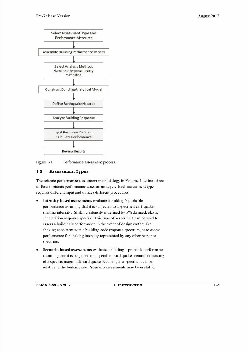
Figure 1-1 illustrates the basic steps in the performance assessment process.
Volume 1 describes each of these steps and how they relate to the overall
performance assessment. Three of these steps, assembling building
performance model, defining earthquake hazards, and analyzing building
response; in addition to developing collapse fragility, when necessary, are
performed directly by the user. In the implementations described in this
guide, the performance is calculated by PACT.
8/12/2019 Seismic Performance Assessment of Buildings
http://slidepdf.com/reader/full/seismic-performance-assessment-of-buildings 25/358
Pre-Release Version August 2012
FEMA P-58 – Vol. 2 1: Introduction 1-3
Figure 1-1 Performance assessment process.
1.5 Assessment Types
The seismic performance assessment methodology in Volume 1 defines three
different seismic performance assessment types. Each assessment type
requires different input and utilizes different procedures.
Intensity-based assessments evaluate a building’s probable
performance assuming that it is subjected to a specified earthquake
shaking intensity. Shaking intensity is defined by 5% damped, elastic
acceleration response spectra. This type of assessment can be used to
assess a building’s performance in the event of design earthquake
shaking consistent with a building code response spectrum, or to assess performance for shaking intensity represented by any other response
spectrum.
Scenario-based assessments evaluate a building’s probable performance
assuming that it is subjected to a specified earthquake scenario consisting
of a specific magnitude earthquake occurring at a specific location
relative to the building site. Scenario assessments may be useful for

8/12/2019 Seismic Performance Assessment of Buildings
http://slidepdf.com/reader/full/seismic-performance-assessment-of-buildings 26/358
August 2012 Pre-Release Version
1-4 1: Introduction FEMA P-58 – Vol. 2
buildings located close to one or more known active faults. This type of
assessment can be used to assess a building’s performance in the event of
a historic earthquake on these faults is repeated, or a future projected
earthquake occurs.
Time-based assessments evaluate a building’s probable performanceover a specified period of time (e.g., 1-year, 30-years, or 50-years)
considering all the earthquakes that could occur in that time period, and
the probability of occurrence associated with each earthquake. Time-
based assessments consider uncertainty in the magnitude and location of
future earthquakes as well as the intensity of motion resulting from these
earthquakes.
1.6 Performance Measures
The seismic performance of a building is expressed as the probable damage
and resulting consequences of a building’s response to earthquake shaking.
The consequences, or impacts, resulting from earthquake damage considered
in this methodology are:
Casualties. Loss of life, or serious injury requiring hospitalization,
occurring within the building envelope;
Repair cost. The cost, in present dollars, necessary to restore a building
to its pre-earthquake condition, or in the case of total loss, to replace the
building with a new structure of similar construction;
Repair time. The time, in weeks, necessary to repair a damaged
building to its pre-earthquake condition; and
Unsafe placarding. A post-earthquake inspection rating that deems a
building, or portion of a building, damaged to the point that entry, use, or
occupancy poses immediate risk to safety.
Each performance measure requires basic information about the building’s
characteristics.
1.7 Analysis Methods
The methodology provides users with a range of options for generating theabove assessments. The options include use of a simplified analytical
estimation of building response or suites of detailed nonlinear response-
history analyses. The building assets at risk can be defined by occupancy-
dependent typical (normative) quantities or building-specific surveys. The
performance characteristics of these at-risk assets can be represented by
provided relationships for component fragility and consequences, or
8/12/2019 Seismic Performance Assessment of Buildings
http://slidepdf.com/reader/full/seismic-performance-assessment-of-buildings 27/358
Pre-Release Version August 2012
FEMA P-58 – Vol. 2 1: Introduction 1-5
component-specific fragility and consequence functions can be developed
and used. Each building performance assessment can use either of the
analysis approaches or any combination of the options to define component
fragility and consequence characteristics.
The simplest application of the methodology includes use of the simplifiedanalysis method to estimate building response and the selection of provided,
occupancy-dependent, fragility and consequence functions for the building
assets at risk. This streamlined approach may be most appropriate for
circumstances where information about the building’s characteristics is
limited as is typical during preliminary design of new buildings or in the
initial evaluation stages for existing buildings. In general, the more
streamlined the approach, the more limitations there are in the methodology’s
ability to characterize performance and the larger the inherent uncertainty in
the performance assessments.
1.8 Document Organization
The Implementation Guide is organized into the following chapters:
Chapter 2 provides a detailed description of the steps used to develop a
building performance model consisting of basic building information,
structural and nonstructural fragility specifications, consequence functions,
and the building’s collapse fragility and residual drift characteristics.
Chapter 3 provides a detailed description of the steps required to execute
intensity, scenario, and time-based assessments.
Chapter 4 provides a comprehensive, step-by-step application of the
methodology for an intensity-based assessment that uses simplified analysis
for estimating building response and relies on provided fragility and
consequence functions to characterize component vulnerability.
Chapter 5 provides a comprehensive step-by-step application of the
methodology for time-based assessment using response history analyses to
estimate building response and the performance assessment model developed
in Chapter 4 with minor modifications.
Chapter 6 illustrates development of structural component fragility functions
by calculation to address unique circumstances or to supplement the
available provided fragility functions.
Chapter 7 illustrates development of nonstructural component fragility
functions by calculation to address unique circumstances or to supplement
the available provided fragility functions.
8/12/2019 Seismic Performance Assessment of Buildings
http://slidepdf.com/reader/full/seismic-performance-assessment-of-buildings 28/358
August 2012 Pre-Release Version
1-6 1: Introduction FEMA P-58 – Vol. 2
Chapter 8 provides guidance on the development of component consequence
functions to accompany user-defined fragility functions and to supplement or
modify provided consequence functions.
The following appendices are included with the guide:
Appendix A provides a compilation of provided fragility specifications for
structural components.
Appendix B provides a compilation of provided fragility specifications for
nonstructural components.
Appendix C provides the user’s manual of instructions for the Performance
Assessment Calculation Tool (PACT).
Appendix D describes the Normative Quantity Estimation tool that is
designed to assist in estimating the type and quantity of nonstructural
components typically present in buildings of a given occupancy and size.
References and the list of project participants are provided at the end of this
report.
8/12/2019 Seismic Performance Assessment of Buildings
http://slidepdf.com/reader/full/seismic-performance-assessment-of-buildings 29/358
Pre-Release Version August 2012
FEMA P-58 – Vol. 2 2: Building Performance Modeling 2-1
Chapter 2
Building Performance Modeling
2.1 Introduction
This chapter provides guidance for assembling the building performance
model and is organized to provide direct references to the appropriate input
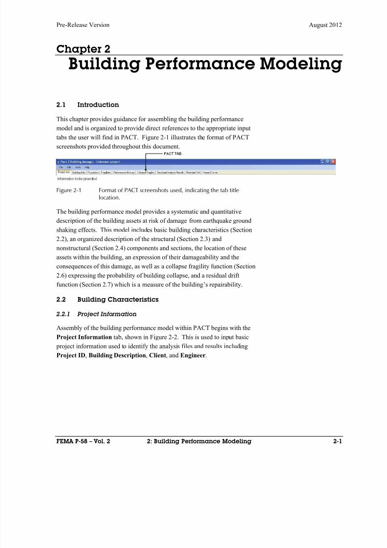
tabs the user will find in PACT. Figure 2-1 illustrates the format of PACT
screenshots provided throughout this document.
Figure 2-1 Format of PACT screenshots used, indicating the tab titlelocation.
The building performance model provides a systematic and quantitative
description of the building assets at risk of damage from earthquake ground
shaking effects. This model includes basic building characteristics (Section
2.2), an organized description of the structural (Section 2.3) and
nonstructural (Section 2.4) components and sections, the location of these
assets within the building, an expression of their damageability and the
consequences of this damage, as well as a collapse fragility function (Section2.6) expressing the probability of building collapse, and a residual drift
function (Section 2.7) which is a measure of the building’s repairability.
2.2 Building Characteristics
2.2.1 Project Information
Assembly of the building performance model within PACT begins with the
Project Information tab, shown in Figure 2-2. This is used to input basic
project information used to identify the analysis files and results including
Project ID, Building Description, Client, and Engineer.
8/12/2019 Seismic Performance Assessment of Buildings
http://slidepdf.com/reader/full/seismic-performance-assessment-of-buildings 30/358
August 2012 Pre-Release Version
2-2 2: Building Performance Modeling FEMA P-58-1 – Vol. 2
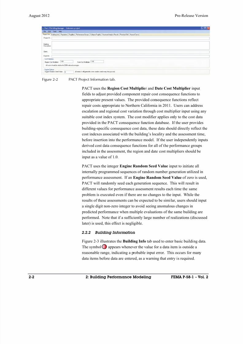
Figure 2-2 PACT Project Information tab.
PACT uses the Region Cost Multiplier and Date Cost Multiplier input
fields to adjust provided component repair cost consequence functions to
appropriate present values. The provided consequence functions reflect
repair costs appropriate to Northern California in 2011. Users can address
escalation and regional cost variation through cost multiplier input using anysuitable cost index system. The cost modifier applies only to the cost data
provided in the PACT consequence function database. If the user provides
building-specific consequence cost data, these data should directly reflect the
cost indexes associated with the building’s locality and the assessment time,
before insertion into the performance model. If the user independently inputs
derived cost data consequence functions for all of the performance groups
included in the assessment, the region and date cost multipliers should be
input as a value of 1.0.
PACT uses the integer Engine Random Seed Value input to initiate all
internally programmed sequences of random number generation utilized in
performance assessment. If an Engine Random Seed Value of zero is used,
PACT will randomly seed each generation sequence. This will result in
different values for performance assessment results each time the same
problem is executed even if there are no changes to the input. While the
results of these assessments can be expected to be similar, users should input
a single digit non-zero integer to avoid seeing anomalous changes in
predicted performance when multiple evaluations of the same building are
performed. Note that if a sufficiently large number of realizations (discussed
later) is used, this effect is negligible.
2.2.2 Building Information
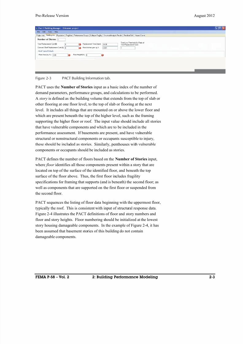
Figure 2-3 illustrates the Building Info tab used to enter basic building data.
The symbol appears whenever the value for a data item is outside a
reasonable range, indicating a probable input error. This occurs for many
data items before data are entered, as a warning that entry is required.
8/12/2019 Seismic Performance Assessment of Buildings
http://slidepdf.com/reader/full/seismic-performance-assessment-of-buildings 31/358
Pre-Release Version August 2012
FEMA P-58 – Vol. 2 2: Building Performance Modeling 2-3
Figure 2-3 PACT Building Information tab.
PACT uses the Number of Stories input as a basic index of the number of
demand parameters, performance groups, and calculations to be performed.
A story is defined as the building volume that extends from the top of slab or
other flooring at one floor level, to the top of slab or flooring at the next
level. It includes all things that are mounted on or above the lower floor and
which are present beneath the top of the higher level, such as the framing
supporting the higher floor or roof. The input value should include all stories
that have vulnerable components and which are to be included in the
performance assessment. If basements are present, and have vulnerable
structural or nonstructural components or occupants susceptible to injury,
these should be included as stories. Similarly, penthouses with vulnerable
components or occupants should be included as stories.
PACT defines the number of floors based on the Number of Stories input,
where floor identifies all those components present within a story that are
located on top of the surface of the identified floor, and beneath the top
surface of the floor above. Thus, the first floor includes fragility
specifications for framing that supports (and is beneath) the second floor; as
well as components that are supported on the first floor or suspended from
the second floor.
PACT sequences the listing of floor data beginning with the uppermost floor,
typically the roof. This is consistent with input of structural response data.
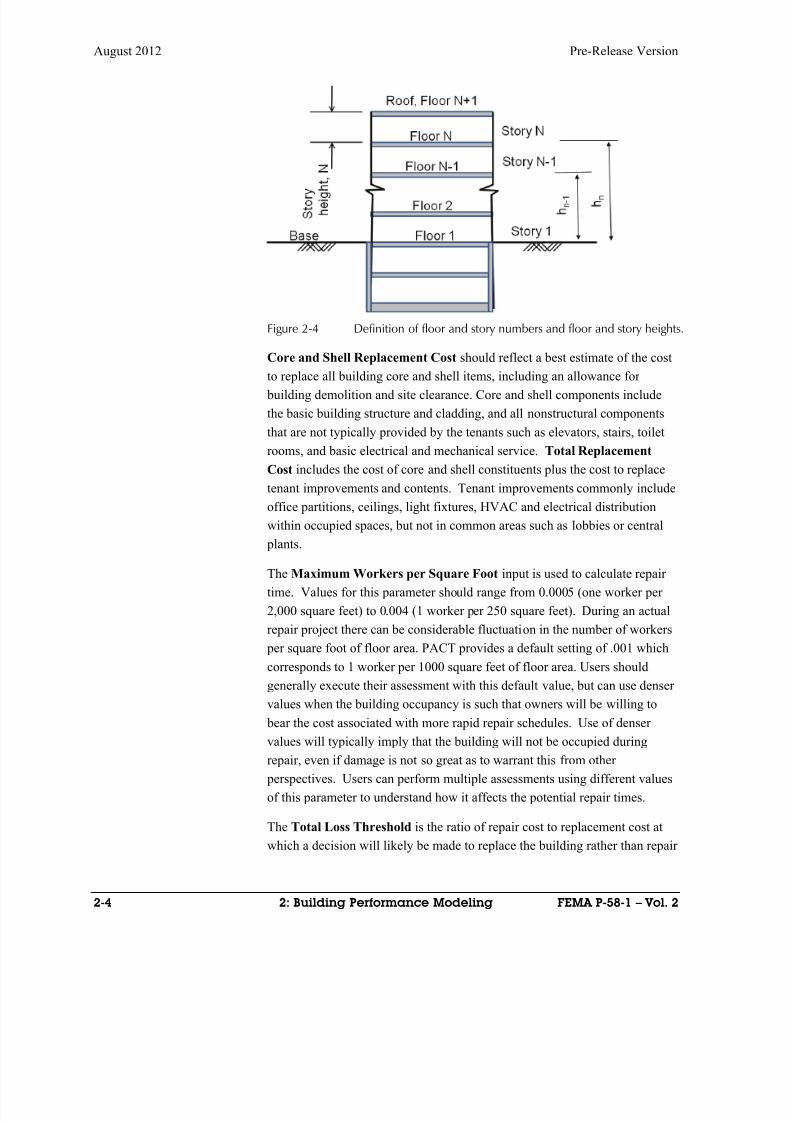
Figure 2-4 illustrates the PACT definitions of floor and story numbers and
floor and story heights. Floor numbering should be initialized at the lowest
story housing damageable components. In the example of Figure 2-4, it has been assumed that basement stories of this building do not contain
damageable components.
8/12/2019 Seismic Performance Assessment of Buildings
http://slidepdf.com/reader/full/seismic-performance-assessment-of-buildings 32/358
August 2012 Pre-Release Version
2-4 2: Building Performance Modeling FEMA P-58-1 – Vol. 2
Figure 2-4 Definition of floor and story numbers and floor and story heights.
Core and Shell Replacement Cost should reflect a best estimate of the cost
to replace all building core and shell items, including an allowance for
building demolition and site clearance. Core and shell components include
the basic building structure and cladding, and all nonstructural components
that are not typically provided by the tenants such as elevators, stairs, toilet
rooms, and basic electrical and mechanical service. Total Replacement
Cost includes the cost of core and shell constituents plus the cost to replace
tenant improvements and contents. Tenant improvements commonly include
office partitions, ceilings, light fixtures, HVAC and electrical distribution
within occupied spaces, but not in common areas such as lobbies or central
plants.
The Maximum Workers per Square Foot input is used to calculate repair
time. Values for this parameter should range from 0.0005 (one worker per
2,000 square feet) to 0.004 (1 worker per 250 square feet). During an actual
repair project there can be considerable fluctuation in the number of workers
per square foot of floor area. PACT provides a default setting of .001 which
corresponds to 1 worker per 1000 square feet of floor area. Users should
generally execute their assessment with this default value, but can use denser
values when the building occupancy is such that owners will be willing to
bear the cost associated with more rapid repair schedules. Use of denser
values will typically imply that the building will not be occupied during
repair, even if damage is not so great as to warrant this from other
perspectives. Users can perform multiple assessments using different values
of this parameter to understand how it affects the potential repair times.
The Total Loss Threshold is the ratio of repair cost to replacement cost at
which a decision will likely be made to replace the building rather than repair
8/12/2019 Seismic Performance Assessment of Buildings
http://slidepdf.com/reader/full/seismic-performance-assessment-of-buildings 33/358
Pre-Release Version August 2012
FEMA P-58 – Vol. 2 2: Building Performance Modeling 2-5
it. FEMA uses a value of 0.5 for this loss ratio when determining whether
post-earthquake repair projects should be funded and to what extent. PACT
uses a default value of 1.0 to maximize the amount of assessment
information that will be obtained in an assessment. Volume 1 suggests that
when the repair costs exceed 40% of replacement costs, many owners will
choose to demolish the existing building and replace it with a new one.
Floor Area input is used to determine the number of people present in the
building during an earthquake realization to estimate the number of
casualties. Floor Height is not presently used within PACT, but must be
input anyway. Any reasonable value can be input. This information placed
in the Most Typical Default section of the tab is used by PACT to populate
a matrix of values for each floor, identified in the lower portion of the tab.
PACT will initialize this matrix with the value entered for the Most Typical
Values section above. Users can change these values by entering other
values directly into the individual cells of the matrix.
The Height Factor is used to reflect increases in repair cost attributable to:
Loss of efficiency due to added travel time to get to damaged
components on upper levels
Material and tool loading and staging, including added cost for hoisting,
elevator loading, pumping, and disposal
Access costs related to cutting openings or penetrations, or window
removal, to permit material loading and movement to installation areas
Scaffolding or rigging, including fall protection and protection to lower
areas
Minor cost adjustments may be appropriate for simple interior repairs, where
the impact is a minor loss of efficiency for worker elevator travel. Significant
adjustments may be necessary for exterior cladding repairs on a high rise
building which could require significant scaffolding for an otherwise low
cost repair item. Both of these extremes are unlikely to produce a significant
total repair cost error, since they are typically combined with much less
sensitive work items. While there can be a significant range of height
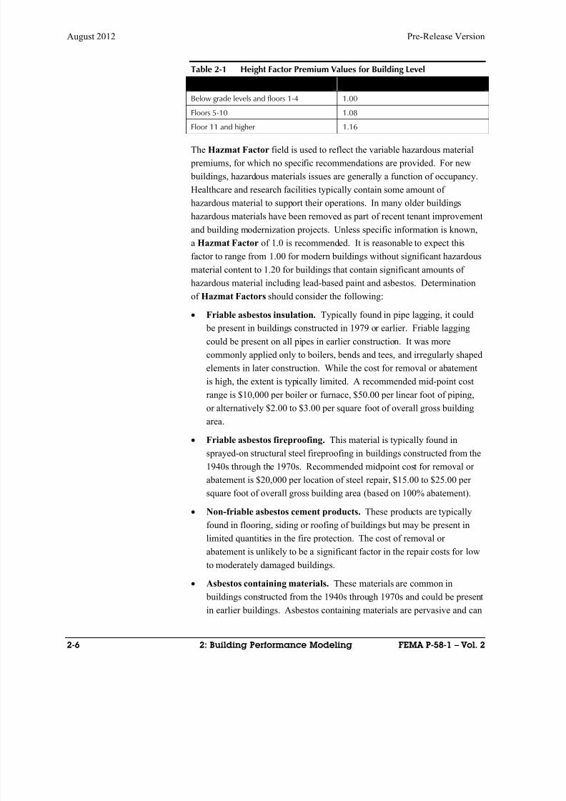
premium costs for individual items, the aggregated modifications will be arelatively small increase for most cases. Table 2-1 presents suggested Height
Factor premiums.
8/12/2019 Seismic Performance Assessment of Buildings
http://slidepdf.com/reader/full/seismic-performance-assessment-of-buildings 34/358
August 2012 Pre-Release Version
2-6 2: Building Performance Modeling FEMA P-58-1 – Vol. 2
Table 2-1 Height Factor Premium Values for Building Level
Building Level Height Factor
Below grade levels and floors 1-4 1.00
Floors 5-10 1.08
Floor 11 and higher 1.16
The Hazmat Factor field is used to reflect the variable hazardous material
premiums, for which no specific recommendations are provided. For new
buildings, hazardous materials issues are generally a function of occupancy.
Healthcare and research facilities typically contain some amount of
hazardous material to support their operations. In many older buildings
hazardous materials have been removed as part of recent tenant improvement
and building modernization projects. Unless specific information is known,
a Hazmat Factor of 1.0 is recommended. It is reasonable to expect this
factor to range from 1.00 for modern buildings without significant hazardous
material content to 1.20 for buildings that contain significant amounts of
hazardous material including lead-based paint and asbestos. Determination
of Hazmat Factors should consider the following:
Friable asbestos insulation. Typically found in pipe lagging, it could
be present in buildings constructed in 1979 or earlier. Friable lagging
could be present on all pipes in earlier construction. It was more
commonly applied only to boilers, bends and tees, and irregularly shaped
elements in later construction. While the cost for removal or abatement
is high, the extent is typically limited. A recommended mid-point cost
range is $10,000 per boiler or furnace, $50.00 per linear foot of piping,or alternatively $2.00 to $3.00 per square foot of overall gross building
area.
Friable asbestos fireproofing. This material is typically found in
sprayed-on structural steel fireproofing in buildings constructed from the
1940s through the 1970s. Recommended midpoint cost for removal or
abatement is $20,000 per location of steel repair, $15.00 to $25.00 per
square foot of overall gross building area (based on 100% abatement).
Non-friable asbestos cement products. These products are typically
found in flooring, siding or roofing of buildings but may be present inlimited quantities in the fire protection. The cost of removal or
abatement is unlikely to be a significant factor in the repair costs for low
to moderately damaged buildings.
Asbestos containing materials. These materials are common in
buildings constructed from the 1940s through 1970s and could be present
in earlier buildings. Asbestos containing materials are pervasive and can
8/12/2019 Seismic Performance Assessment of Buildings
http://slidepdf.com/reader/full/seismic-performance-assessment-of-buildings 35/358
Pre-Release Version August 2012
FEMA P-58 – Vol. 2 2: Building Performance Modeling 2-7
be found in ceiling tiles, spray acoustic treatment, flooring materials,
floor mastic, roofing materials, caulk and drywall taping compound. The
midpoint cost for removal or abatement is approximately $10.00 to
$30.00 per square foot of overall gross building area.
Poly chlorinated biphenols. This material is commonly found inelectrical equipment that includes fluorescent light ballasts and caulk.
Poly chlorinated biphenols (PCB) could be present in buildings
constructed before 1991, but are more likely present in construction
preceding 1980. In many cases PCB ballasts have been replaced during
energy retrofits, so older buildings may not necessarily contain PCB
materials.
The following midpoint costs are suggested:
o Ballast replacement in damaged fixtures: $100 per fixture. Ballasts
in undamaged fixtures should not need to be replaced following anearthquake.
o Other electrical equipment (transformers, switchgear): premium cost
in addition to equipment replacement: $20,000 per item.
o PCB containing caulk has only recently been recognized as a
significant environmental problem. Repair protocols are not well
established. PCB can migrate from the caulk into surrounding porous
materials. This could necessitate not only caulk removal, but also
replacement of surrounding materials, such as masonry, concrete
wood, etc. The midpoint costs suggested are for recaulking only andfor abatement or removal is $15.00 per linear foot or $3.00 to $5.00
per square foot of overall gross building area.
Lead based paint. In buildings constructed prior to 1980, painted
surfaces particularly, wood and steel, are likely to contain lead based
paint. Midpoint cost for removal or abatement is $3.00 per square foot
of painted area, or $2.00 to $5.00 for multi-unit residential and education
facilities, and $5.00 to $8.00 per square foot of overall building area for
complete structural steel abatement. For structural steel, it may be more
useful to use $5,000 per repair location.
There are many other hazardous materials and conditions that could be
encountered in repair efforts. Typically these treatments are inconsequential
from a cost perspective, in the larger context of seismic repair. These
materials can include mercury in light fixtures and switching devices
(thermostats), dry-cleaning fluids, gasoline or diesel or other hydrocarbons in
generators or fuel storage tanks, chemicals from process or manufacturing,

8/12/2019 Seismic Performance Assessment of Buildings
http://slidepdf.com/reader/full/seismic-performance-assessment-of-buildings 36/358
August 2012 Pre-Release Version
2-8 2: Building Performance Modeling FEMA P-58-1 – Vol. 2
and radioactive materials (particularly in healthcare or laboratory
equipment).
The Occupancy Factor reflects the added cost of working around ongoing
building operations, equipment and the collateral protections required for
some construction characteristics. The occupancy premium is significantlymore pronounced in occupied buildings than in vacated buildings. However,
the level of collateral protection required even in an unoccupied building
may be significant. Table 2-2 lists recommended repair premiums for typical
occupied and unoccupied buildings. PACT does not presently distinguish
between occupied and unoccupied repair conditions.
For time-based assessments, unoccupied factors should be used. For
scenario- and intensity-based assessments, factors appropriate to “occupied”
should be used for low intensity shaking since repair of minor damage is
likely to be done with the building occupied. For moderate to high levels ofshaking intensity, the use of the unoccupied factors is recommended as
buildings are more likely to be damaged beyond a level at which repair
during occupancy is practical.
Table 2-2 Occupancy Factors
Occupancy Category Occupancy Factor
Unoccupied Occupied
Commercial Office 1.0 1.2
Research 1.4 1.8
Healthcare 1.5 2.0
Education K-12 1.0 1.1
Multi-Unit Residential 1.1 1.2
Retail 1.2 1.3
Warehouse 1.1 1.1
Hospitality 1.1 1.3
2.2.3 Population Model
To assess casualties, users must define the distribution of occupants within
the building (Figure 2-5) at various times of day, termed the populationmodel. It is possible to use one of the provided building population models
or to develop and input building-specific models. Eight population models
are provided in PACT corresponding to typical Commercial Office,
Education K-12 (Elementary, Middle, High School), Healthcare, Hospitality,
Multi-Unit Residential, Research, Retail and Warehouse occupancies.

8/12/2019 Seismic Performance Assessment of Buildings
http://slidepdf.com/reader/full/seismic-performance-assessment-of-buildings 37/358
Pre-Release Version August 2012
FEMA P-58 – Vol. 2 2: Building Performance Modeling 2-9
Users can assign separate population models to several fractions of each floor
level. Each population model includes the hourly distribution of people per
1,000 square feet for weekdays or weekends and can be adjusted to include
further variation by month. Provided population models can be used directly
or be modified to reflect the unique occupancy characteristics of a specific
building, if known. Figure 2-5 illustrates the commercial office occupancy
provided in PACT. Building-specific population information can be
developed and modified using the Population Manager utility, as illustrated
in Figure 2-6. The existing population models for each occupancy category
can be viewed by selecting from the column on the left. Modifications can be
made to the provided models by substituting data on the right side of the
window. New occupancies can be created by overwriting the existing ones or
creating new names for the occupancy.
Figure 2-5 PACT Population tab showing commercial office occupancy.

8/12/2019 Seismic Performance Assessment of Buildings
http://slidepdf.com/reader/full/seismic-performance-assessment-of-buildings 38/358
August 2012 Pre-Release Version
2-10 2: Building Performance Modeling FEMA P-58-1 – Vol. 2
Figure 2-6 PACT Population Manager utility.
2.3 Fragility Specifications and Performance Groups
Following the definition of the general building characteristics, it is
necessary to define the quantity, vulnerability and distribution of damageable
components and contents. For any particular building component, e.g. a
structural brace, information about the component’s damageability and the
possible consequences of any damage incurred is termed a fragility
specification.
PACT organizes this process into two parts: (1) identification of required
fragility specifications for each floor/story, and (2) identification of the
quantity of components in each performance group at each floor/story. Each
performance group consists of the set of components having the same
fragility specification and that are assumed to experience the same demands.
PACT includes a data set of more than 700 individual fragility specifications
for common building items, containing both structural and nonstructural
components. Components can be selected and distributed across the
building’s floor plates to create a complete representation of the damageable
building.
Users should be aware that the fragility specification library provided with
PACT does not include all vulnerable building components that may be
present in a building. Users must be careful to identify damageable building
features not addressed in the PACT fragility specifications or the Normative
Quantity Estimation tool. User-defined fragility and consequence functions
can be developed following the guidance provided in Chapters 6, 7, and 8.
8/12/2019 Seismic Performance Assessment of Buildings
http://slidepdf.com/reader/full/seismic-performance-assessment-of-buildings 39/358
Pre-Release Version August 2012
FEMA P-58 – Vol. 2 2: Building Performance Modeling 2-11
Many building components are inherently rugged. Rugged components
include such things as plumbing fixtures, electrical raceways, wall-mounted
panels, and some components of gravity framing systems. Volume 1
Appendix I includes an itemized listing of common building components that
can generally be considered rugged. These components are not typically
susceptible to damage as a result of a building’s earthquake response, and
need not be included in the building performance model.
Figure 2-7 illustrates the PACT screen used to identify the fragility
specifications present in a performance model. Table 2-3 provides a list of
fragility specifications identified in PACT. Fragility specifications provided
in the PACT database are identified with bold lettering in Table 2-3.
Each fragility specification is identified by a unique identification code based
on NISTIR 6389 Report, UNIFORMAT II Elemental Classification for
Building Specifications, Cost Estimating and Cost Analysis (NIST, 1999)where codes take the form: A1234.567. The first letter in the classification
system indicates the overall component category. The first two numbers
provides the next categorization. For instance, B10 represents superstructure
components while B20 represents exterior enclosures. The next two numbers
identify a unique component. For example, the classification for reinforced
concrete shear walls is B1044. The identifiers after the decimal provide
variations of the basic component and are used to identify different
configurations, conditions of installation, material quantities, demand levels,
and other attributes.
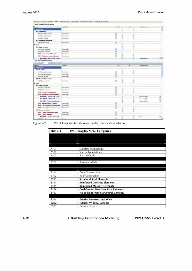
8/12/2019 Seismic Performance Assessment of Buildings
http://slidepdf.com/reader/full/seismic-performance-assessment-of-buildings 40/358
August 2012 Pre-Release Version
2-12 2: Building Performance Modeling FEMA P-58-1 – Vol. 2
Figure 2-7 PACT Fragilities tab showing fragility specification selection.
Table 2-3 PACT Fragility Menu Categories
Fragility ClassificationNumber Component / System
A Substructure
A10 Foundation
A101 Standard Foundations
A102 Special Foundations
A103 Slab on Grade
A20 Basement Construction
A202 Basement Walls
B Superstructure
B10 Superstructure
B101 Floor Construction
B102 Roof Construction
B103 Structural Steel Elements
B104 Reinforced Concrete Elements
B105 Reinforced Masonry Elements
B106 Cold-formed Steel Structural Elements
B107 Wood Light Frame Structural Elements
B20 Exterior Enclosure
B201 Exterior Nonstructural Walls
B202 Exterior Window Systems
B203 Exterior Doors
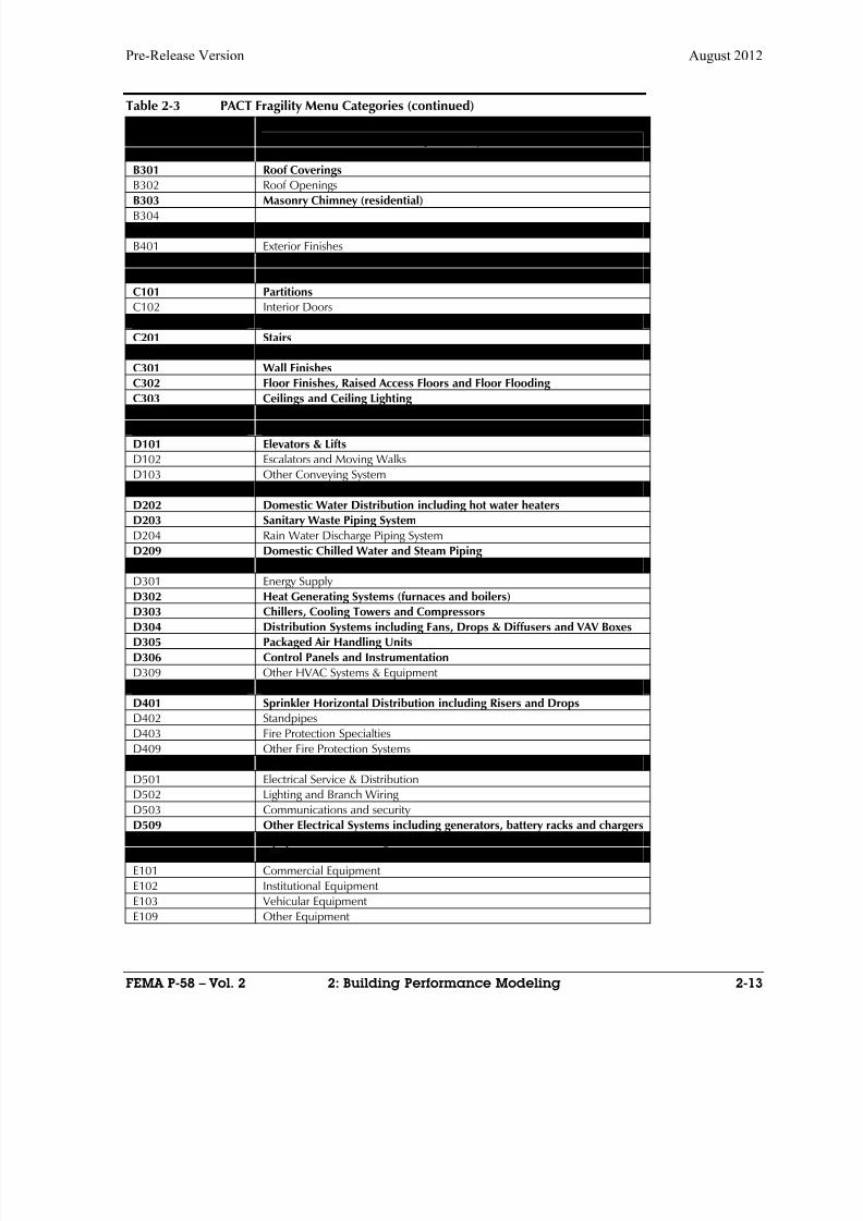
8/12/2019 Seismic Performance Assessment of Buildings
http://slidepdf.com/reader/full/seismic-performance-assessment-of-buildings 41/358
Pre-Release Version August 2012
FEMA P-58 – Vol. 2 2: Building Performance Modeling 2-13
Table 2-3 PACT Fragility Menu Categories (continued)
Fragility ClassificationNumber Component / System
B30 Roof ElementsB301 Roof Coverings
B302 Roof Openings
B303 Masonry Chimney (residential)B304
B40 Exterior Finishes
B401 Exterior Finishes
C Interiors
C10 Interior Construction
C101 Partitions
C102 Interior Doors
C20 Stairs
C201 Stairs
C30 Interior Finishes
C301 Wall Finishes
C302 Floor Finishes, Raised Access Floors and Floor Flooding
C303 Ceilings and Ceiling LightingD Services
D10 Conveying
D101 Elevators & Lifts
D102 Escalators and Moving Walks
D103 Other Conveying System
D20 Plumbing
D202 Domestic Water Distribution including hot water heaters
D203 Sanitary Waste Piping System
D204 Rain Water Discharge Piping System
D209 Domestic Chilled Water and Steam Piping
D30 HVAC
D301 Energy Supply
D302 Heat Generating Systems (furnaces and boilers)D303 Chillers, Cooling Towers and Compressors
D304 Distribution Systems including Fans, Drops & Diffusers and VAV Boxes
D305 Packaged Air Handling Units
D306 Control Panels and Instrumentation
D309 Other HVAC Systems & Equipment
D40 Fire Protection
D401 Sprinkler Horizontal Distribution including Risers and Drops
D402 Standpipes
D403 Fire Protection Specialties
D409 Other Fire Protection Systems
D50 Electrical
D501 Electrical Service & Distribution
D502 Lighting and Branch WiringD503 Communications and security
D509 Other Electrical Systems including generators, battery racks and chargers
E Equipment & Furnishings
E10 Equipment
E101 Commercial Equipment
E102 Institutional Equipment
E103 Vehicular Equipment
E109 Other Equipment

8/12/2019 Seismic Performance Assessment of Buildings
http://slidepdf.com/reader/full/seismic-performance-assessment-of-buildings 42/358
August 2012 Pre-Release Version
2-14 2: Building Performance Modeling FEMA P-58-1 – Vol. 2
Table 2-3 PACT Fragility Menu Categories (continued)
Fragility ClassificationNumber Component / System
E20 Furnishings
E201 Fixed Furnishings
E202 Movable Furnishing (including office furniture and equipment, etc)
F Special Construction & DemolitionF10 Special Construction
F101 Special Structures including Storage Racks
F103 Special Construction Systems
F104 Special Facilities
F105 Special Controls and Instrumentation
Note: Bold entries indicate families of fragility specifications provided in PACT
A unique fragility specification is associated with each fragility group. A
PDF file with all of the provided fragility specifications is provided in
Volume 3 in the Fragility Database.
The fragility specification includes description of the demand parameter that predicts damage, the types of damage that can occur, fragility functions that
indicate the probability of incurring each damage state as a function of
demand and consequence functions that indicate the probable values of loss
that will occur as a result of each damage state.
Each fragility function specifies damage state probabilities for a single
demand parameter. Typically, peak story drift ratio or floor acceleration
parameters are used to determine if a component is damaged. The demand
parameter can have a specific orientation with respect to the component
(directional demand) or the demand can be non-directional. For example,
wall elements will typically be damaged by story drift within their plane,
where suspended ceiling systems are susceptible to damage from floor
acceleration independent of horizontal direction. Unanchored nonstructural
components use peak total floor velocity. Users should be aware that floor
acceleration important to the damageability of a component may be
associated with the floor level above the level under consideration. Section
2.6 identifies components that utilize the demand parameter of the floor level
above (generally, ceiling mounted nonstructural components).
User-defined, building-specific fragility functions can use any appropriate
demand parameter. For example, an analyst could decide that beam-column
joint plastic rotation is the best predictor of damage for a particular type of
structural component and could develop fragility functions based on that
parameter. In addition to the fragility function, the fragility specification
includes consequence functions for each of the damage states. If demand
parameters other than story drift ratio, floor acceleration, or velocity are
8/12/2019 Seismic Performance Assessment of Buildings
http://slidepdf.com/reader/full/seismic-performance-assessment-of-buildings 43/358
Pre-Release Version August 2012
FEMA P-58 – Vol. 2 2: Building Performance Modeling 2-15
used, the structural analysis used to estimate building response must provide
values for the selected demand parameters.
The quantity and distribution of damageable components conforming to each
selected fragility specification is entered into PACT through the definition of
performance groups at each floor level. A performance group is a set ofcomponents described by a single fragility group that will experience the
same demand. Performance groups are ordered by the direction of
application of their common demand parameter. Further discussion is
provided in Section 2.4.3 and Section 2.5.
2.4 Identification of Vulnerable Structural Components
and Systems
In addition to elements of the structure’s intended seismic force-resisting
system, damageable structural components should include vulnerable
structural elements normally considered part of the vertical force-resisting
system, only.
Appendix A lists the structural fragility specifications contained in PACT’s
database. The appendix includes 5 tables that span the range of structural
materials from structural steel to wood light frame systems.
Each group of fragility specifications contains multiple selections that reflect
a range of configuration and construction variations affecting seismic
performance characteristics, for example special vs. ordinary masonry walls.
PACT makes further differentiation among some components with identical
damageability but with significant differences in damage state consequences,
such as repair costs, owing to such characteristics as size and finish.
Users should select the most appropriate set of structural fragility
specifications using the descriptions provided in PACT. The PACT
Fragility Specification Manager utility can also facilitate the process of
identifying appropriate fragility specifications. This utility provides general
information on the available fragility specifications and includes a summary
of the demand parameter and characterization of its applicability to demand
directionality and also permits modification of fragility specifications and
definition of new ones.
The PACT database does not include data for horizontal floor or roof
construction components or systems acting as diaphragms. However,
fragility information for some diaphragm components that act as part of the
vertical-force-resisting system such as slab-column joints and steel beam
shear tab connections, is included, as shown in Appendix A. For buildings
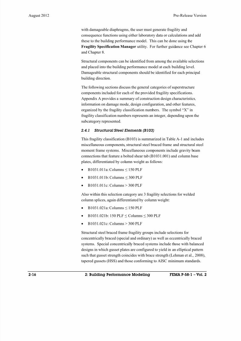
8/12/2019 Seismic Performance Assessment of Buildings
http://slidepdf.com/reader/full/seismic-performance-assessment-of-buildings 44/358
August 2012 Pre-Release Version
2-16 2: Building Performance Modeling FEMA P-58-1 – Vol. 2
with damageable diaphragms, the user must generate fragility and
consequence functions using either laboratory data or calculations and add
these to the building performance model. This can be done using the
Fragility Specification Manager utility. For further guidance see Chapter 6
and Chapter 8.
Structural components can be identified from among the available selections
and placed into the building performance model at each building level.
Damageable structural components should be identified for each principal
building direction.
The following sections discuss the general categories of superstructure
components included for each of the provided fragility specifications.
Appendix A provides a summary of construction design characteristics,
information on damage mode, design configuration, and other features,
organized by the fragility classification numbers. The symbol “X” infragility classification numbers represents an integer, depending upon the
subcategory represented.
2.4.1 Structural Steel Elements (B103)
This fragility classification (B103) is summarized in Table A-1 and includes
miscellaneous components, structural steel braced frame and structural steel
moment frame systems. Miscellaneous components include gravity beam
connections that feature a bolted shear tab (B1031.001) and column base
plates, differentiated by column weight as follows:
B1031.011a: Columns ≤ 150 PLF
B1031.011b: Columns ≤ 300 PLF
B1031.011c: Columns > 300 PLF
Also within this selection category are 3 fragility selections for welded
column splices, again differentiated by column weight:
B1031.021a: Columns ≤ 150 PLF
B1031.021b: 150 PLF ≤ Columns ≤ 300 PLF
B1031.021c: Columns > 300 PLF
Structural steel braced frame fragility groups include selections for
concentrically braced (special and ordinary) as well as eccentrically braced
systems. Special concentrically braced systems include those with balanced
designs in which gusset plates are configured to yield in an elliptical pattern
such that gusset strength coincides with brace strength (Lehman et al., 2008),
tapered gussets (HSS) and those conforming to AISC minimum standards.
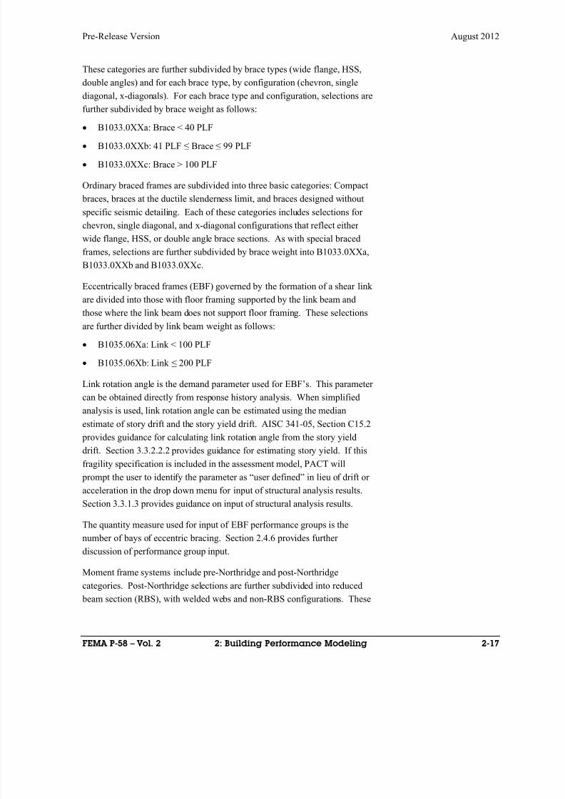
8/12/2019 Seismic Performance Assessment of Buildings
http://slidepdf.com/reader/full/seismic-performance-assessment-of-buildings 45/358
Pre-Release Version August 2012
FEMA P-58 – Vol. 2 2: Building Performance Modeling 2-17
These categories are further subdivided by brace types (wide flange, HSS,
double angles) and for each brace type, by configuration (chevron, single
diagonal, x-diagonals). For each brace type and configuration, selections are
further subdivided by brace weight as follows:
B1033.0XXa: Brace < 40 PLF
B1033.0XXb: 41 PLF ≤ Brace ≤ 99 PLF
B1033.0XXc: Brace > 100 PLF
Ordinary braced frames are subdivided into three basic categories: Compact
braces, braces at the ductile slenderness limit, and braces designed without
specific seismic detailing. Each of these categories includes selections for
chevron, single diagonal, and x-diagonal configurations that reflect either
wide flange, HSS, or double angle brace sections. As with special braced
frames, selections are further subdivided by brace weight into B1033.0XXa,
B1033.0XXb and B1033.0XXc.
Eccentrically braced frames (EBF) governed by the formation of a shear link
are divided into those with floor framing supported by the link beam and
those where the link beam does not support floor framing. These selections
are further divided by link beam weight as follows:
B1035.06Xa: Link < 100 PLF
B1035.06Xb: Link ≤ 200 PLF
Link rotation angle is the demand parameter used for EBF’s. This parameter
can be obtained directly from response history analysis. When simplified
analysis is used, link rotation angle can be estimated using the median
estimate of story drift and the story yield drift. AISC 341-05, Section C15.2
provides guidance for calculating link rotation angle from the story yield
drift. Section 3.3.2.2.2 provides guidance for estimating story yield. If this
fragility specification is included in the assessment model, PACT will
prompt the user to identify the parameter as “user defined” in lieu of drift or
acceleration in the drop down menu for input of structural analysis results.
Section 3.3.1.3 provides guidance on input of structural analysis results.
The quantity measure used for input of EBF performance groups is thenumber of bays of eccentric bracing. Section 2.4.6 provides further
discussion of performance group input.
Moment frame systems include pre-Northridge and post-Northridge
categories. Post-Northridge selections are further subdivided into reduced
beam section (RBS), with welded webs and non-RBS configurations. These
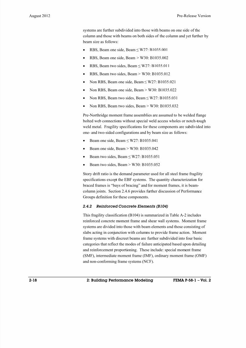
8/12/2019 Seismic Performance Assessment of Buildings
http://slidepdf.com/reader/full/seismic-performance-assessment-of-buildings 46/358
August 2012 Pre-Release Version
2-18 2: Building Performance Modeling FEMA P-58-1 – Vol. 2
systems are further subdivided into those with beams on one side of the
column and those with beams on both sides of the column and yet further by
beam size as follows:
RBS, Beam one side, Beam ≤ W27: B1035.001
RBS, Beam one side, Beam > W30: B1035.002
RBS, Beam two sides, Beam ≤ W27: B1035.011
RBS, Beam two sides, Beam > W30: B1035.012
Non RBS, Beam one side, Beam ≤ W27: B1035.021
Non RBS, Beam one side, Beam > W30: B1035.022
Non RBS, Beam two sides, Beam ≤ W27: B1035.031
Non RBS, Beam two sides, Beam > W30: B1035.032
Pre-Northridge moment frame assemblies are assumed to be welded flange
bolted web connections without special weld access wholes or notch-tough
weld metal. Fragility specifications for these components are subdivided into
one- and two-sided configurations and by beam size as follows:
Beam one side, Beam ≤ W27: B1035.041
Beam one side, Beam > W30: B1035.042
Beam two sides, Beam ≤ W27: B1035.051
Beam two sides, Beam > W30: B1035.052
Story drift ratio is the demand parameter used for all steel frame fragility
specifications except the EBF systems. The quantity characterization for
braced frames is “bays of bracing” and for moment frames, it is beam-
column joints. Section 2.4.6 provides further discussion of Performance
Groups definition for these components.
2.4.2 Reinforced Concrete Elements (B104)
This fragility classification (B104) is summarized in Table A-2 includes
reinforced concrete moment frame and shear wall systems. Moment frame
systems are divided into those with beam elements and those consisting ofslabs acting in conjunction with columns to provide frame action. Moment
frame systems with discreet beams are further subdivided into four basic
categories that reflect the modes of failure anticipated based upon detailing
and reinforcement proportioning. These include: special moment frame
(SMF), intermediate moment frame (IMF), ordinary moment frame (OMF)
and non-conforming frame systems (NCF).
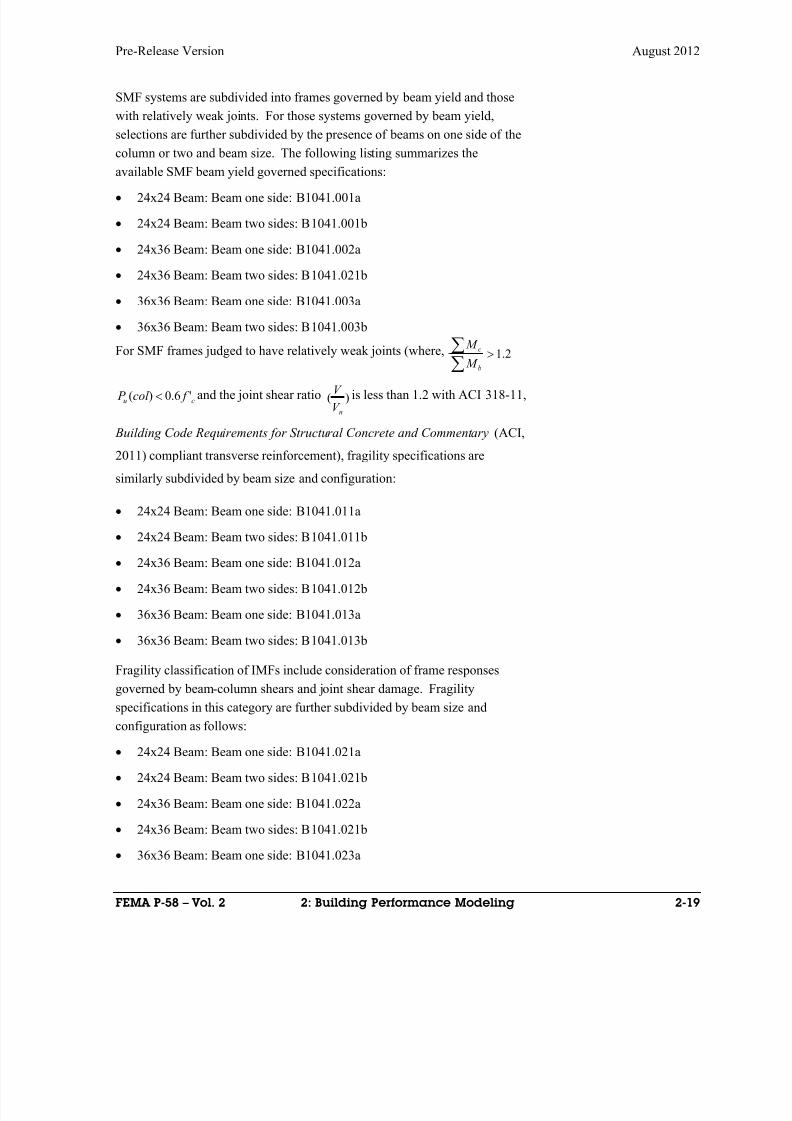
8/12/2019 Seismic Performance Assessment of Buildings
http://slidepdf.com/reader/full/seismic-performance-assessment-of-buildings 47/358
Pre-Release Version August 2012
FEMA P-58 – Vol. 2 2: Building Performance Modeling 2-19
SMF systems are subdivided into frames governed by beam yield and those
with relatively weak joints. For those systems governed by beam yield,
selections are further subdivided by the presence of beams on one side of the
column or two and beam size. The following listing summarizes the
available SMF beam yield governed specifications:
24x24 Beam: Beam one side: B1041.001a
24x24 Beam: Beam two sides: B1041.001b
24x36 Beam: Beam one side: B1041.002a
24x36 Beam: Beam two sides: B1041.021b
36x36 Beam: Beam one side: B1041.003a
36x36 Beam: Beam two sides: B1041.003b
For SMF frames judged to have relatively weak joints (where, 2.1
b
c
M
M
cu f col P '6.0)( and the joint shear ratio )(nV
V is less than 1.2 with ACI 318-11,
Building Code Requirements for Structural Concrete and Commentary (ACI,
2011) compliant transverse reinforcement), fragility specifications are
similarly subdivided by beam size and configuration:
24x24 Beam: Beam one side: B1041.011a
24x24 Beam: Beam two sides: B1041.011b
24x36 Beam: Beam one side: B1041.012a
24x36 Beam: Beam two sides: B1041.012b
36x36 Beam: Beam one side: B1041.013a
36x36 Beam: Beam two sides: B1041.013b
Fragility classification of IMFs include consideration of frame responses
governed by beam-column shears and joint shear damage. Fragility
specifications in this category are further subdivided by beam size and
configuration as follows:
24x24 Beam: Beam one side: B1041.021a
24x24 Beam: Beam two sides: B1041.021b
24x36 Beam: Beam one side: B1041.022a
24x36 Beam: Beam two sides: B1041.021b
36x36 Beam: Beam one side: B1041.023a
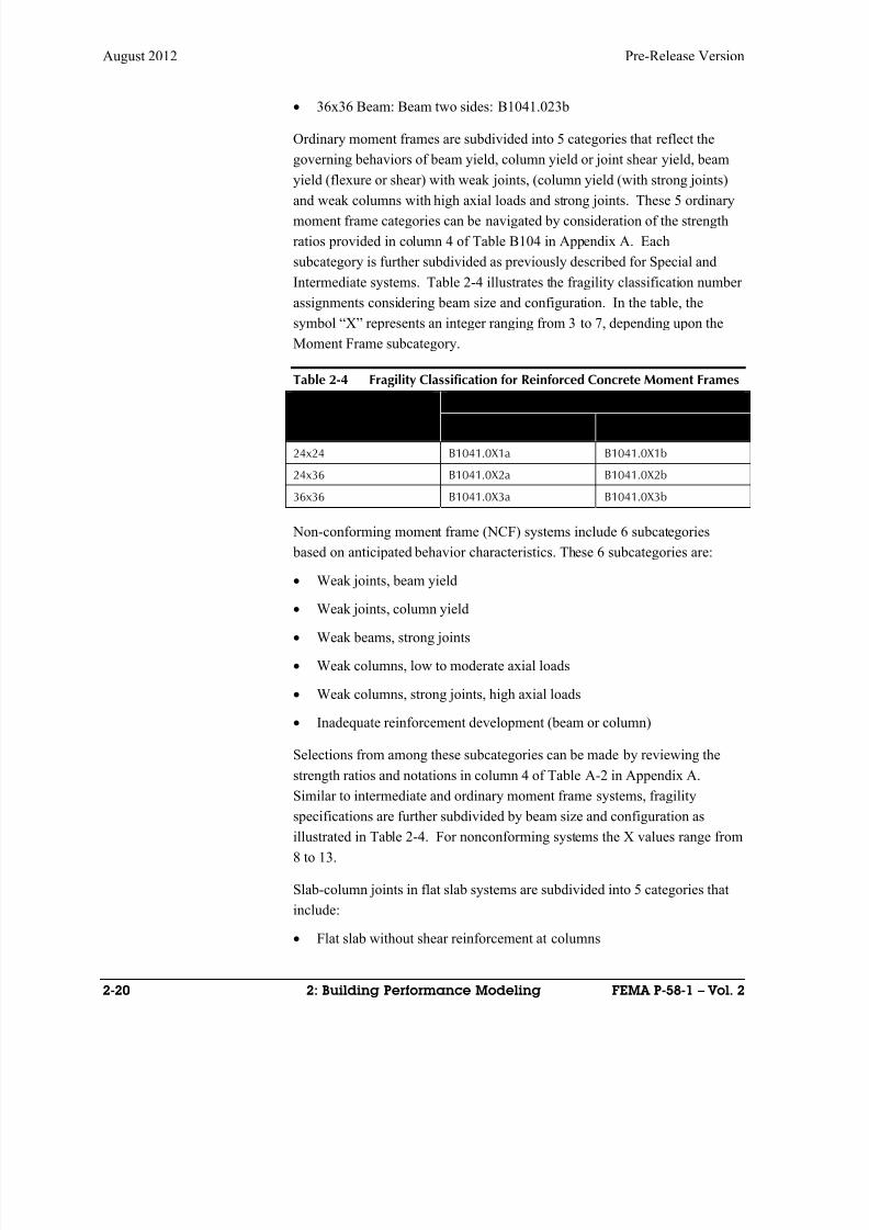
8/12/2019 Seismic Performance Assessment of Buildings
http://slidepdf.com/reader/full/seismic-performance-assessment-of-buildings 48/358
August 2012 Pre-Release Version
2-20 2: Building Performance Modeling FEMA P-58-1 – Vol. 2
36x36 Beam: Beam two sides: B1041.023b
Ordinary moment frames are subdivided into 5 categories that reflect the
governing behaviors of beam yield, column yield or joint shear yield, beam
yield (flexure or shear) with weak joints, (column yield (with strong joints)
and weak columns with high axial loads and strong joints. These 5 ordinarymoment frame categories can be navigated by consideration of the strength
ratios provided in column 4 of Table B104 in Appendix A. Each
subcategory is further subdivided as previously described for Special and
Intermediate systems. Table 2-4 illustrates the fragility classification number
assignments considering beam size and configuration. In the table, the
symbol “X” represents an integer ranging from 3 to 7, depending upon the
Moment Frame subcategory.
Table 2-4 Fragility Classification for Reinforced Concrete Moment Frames
Beam Size Fragility Classification Number
One Sided Two Sided
24x24 B1041.0X1a B1041.0X1b
24x36 B1041.0X2a B1041.0X2b
36x36 B1041.0X3a B1041.0X3b
Non-conforming moment frame (NCF) systems include 6 subcategories
based on anticipated behavior characteristics. These 6 subcategories are:
Weak joints, beam yield
Weak joints, column yield
Weak beams, strong joints
Weak columns, low to moderate axial loads
Weak columns, strong joints, high axial loads
Inadequate reinforcement development (beam or column)
Selections from among these subcategories can be made by reviewing the
strength ratios and notations in column 4 of Table A-2 in Appendix A.
Similar to intermediate and ordinary moment frame systems, fragility
specifications are further subdivided by beam size and configuration as
illustrated in Table 2-4. For nonconforming systems the X values range from
8 to 13.
Slab-column joints in flat slab systems are subdivided into 5 categories that
include:
Flat slab without shear reinforcement at columns

8/12/2019 Seismic Performance Assessment of Buildings
http://slidepdf.com/reader/full/seismic-performance-assessment-of-buildings 49/358
Pre-Release Version August 2012
FEMA P-58 – Vol. 2 2: Building Performance Modeling 2-21
Flat slab with shear reinforcement at columns
Post-tensioned slab without shear reinforcement at columns
Post-tensioned slab with shear reinforcement at columns
Flat slab with drop panel or capital without shear reinforcement at
columns
Each of these subcategories is further subdivided by the ratio of gravity shear
to total shear (factored) and whether integrity reinforcement over columns is
present or not. This results in 18 selections that encompass classification
numbers B1049.001a through B1049.042b.
Story drift ratio is the demand parameter used for all concrete frames. Each
joint (beam or slab to column) is included in tallying damageable
components. For moment frames with beams, separate performance groups
must be designated in each direction. Slab-column moment frame fragilityspecifications use non-directional demands.
Reinforced concrete shear wall systems include squat walls (h/l < 1.0) and
slender walls (h/l ≥ 2.0). Six subcategories of squat walls reflect
reinforcement and configuration options (single curtain or double curtain of
reinforcement and the presence of flanges or boundary columns). These
subcategories are further subdivided based upon wall thickness and height.
Planar single curtain walls include walls 8 inches thick or less at heights
including 15 feet, 16-24 feet or 25-40 corresponding to fragility classification
numbers B1044.001, B1044.002 and B1044.003. Table 2-5 indicates the
fragility categories available for concrete walls with two curtains of
reinforcement:
Table 2-5 Fragility Classification forReinforced Concrete Walls
Thickness Height FragilityClassification
Number
8-16 inches ≤ 15 feet B1044.011
8-16 inches 16 to 24 feet B1044.012
8-16 inches 24 to 40 feet B1044.013
18-24 inches ≤ 15 feet B1044.021
18-24 inches 16 to 24 feet B1044.022
18-24 inches 24 to 40 feet B1044.023
Table 2-6 indicates the further sub-categorization of wall fragility
specifications to account for configurations with return flanges including

8/12/2019 Seismic Performance Assessment of Buildings
http://slidepdf.com/reader/full/seismic-performance-assessment-of-buildings 50/358
August 2012 Pre-Release Version
2-22 2: Building Performance Modeling FEMA P-58-1 – Vol. 2
single curtain and double curtain reinforcement subcategories thickness and
height subdivisions:
Table 2-6 Fragility Classification for Concrete Walls with Return Flanges
Curtains of Reinforcement Thickness Height Fragility
ClassificationNumber
Single 0-8 inches ≤ 15 feet B1044.031
16 to 24 feet B1044.032
24 to 40 feet B1044.033
Double 8-16 inches ≤ 15 feet B1044.041
16 to 24 feet B1044.042
24 to 40 feet B1044.043
16-24 inches ≤ 15 feet B1044.051
16 to 24 feet B1044.052
24 to 40 feet B1044.053
Similar to walls with flanges, walls with boundary columns are subdivided
into categories that reflect single and double curtains of reinforcement, again
further subdivided by thickness and height. Slender walls (with height to
length ratios in excess of 2) are subdivided by thickness (12, 18, and 30
inches) and further subdivided by wall length (15, 20, and 30 feet).
Story drift ratio is the demand parameter for concrete wall systems. Each
wall segment with an aspect ratio within a story of H x H , where H is the story
height is counted as a unit for developing performance group quantities.Section 2.4.6 provides additional discussion of this topic.
2.4.3 Reinforced Masonry Elements (B105)
This category includes fully grouted and partially grouted walls. Each of
these categories is further subdivided into shear dominated or flexure
dominated behavior. Shear dominated walls will fail in shear rather than
yield in flexure. Flexure dominated walls have sufficient shear strength to
force flexural hinging of the wall as a limit state. ACI (2008) equations can
be used to establish the appropriate subcategory selection. Within these
subcategories (shear or flexural dominated) further subdivisions are made based on wall thickness and height as shown in Table 2-7.
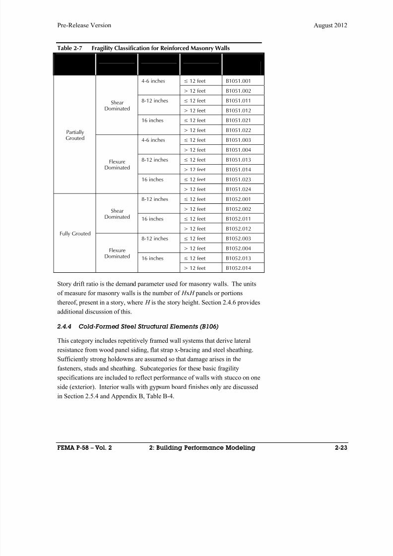
8/12/2019 Seismic Performance Assessment of Buildings
http://slidepdf.com/reader/full/seismic-performance-assessment-of-buildings 51/358
Pre-Release Version August 2012
FEMA P-58 – Vol. 2 2: Building Performance Modeling 2-23
Table 2-7 Fragility Classification for Reinforced Masonry Walls
ConstructionCharacteristics
Damage Mode Thickness Height FragilityClassification
Number
PartiallyGrouted
ShearDominated
4-6 inches ≤ 12 feet B1051.001
> 12 feet B1051.002
8-12 inches ≤ 12 feet B1051.011
> 12 feet B1051.012
16 inches ≤ 12 feet B1051.021
> 12 feet B1051.022
FlexureDominated
4-6 inches ≤ 12 feet B1051.003
> 12 feet B1051.004
8-12 inches ≤ 12 feet B1051.013
> 12 feet B1051.014
16 inches≤
12 feet B1051.023> 12 feet B1051.024
Fully Grouted
ShearDominated
8-12 inches ≤ 12 feet B1052.001
> 12 feet B1052.002
16 inches ≤ 12 feet B1052.011
> 12 feet B1052.012
FlexureDominated
8-12 inches ≤ 12 feet B1052.003
> 12 feet B1052.004
16 inches ≤ 12 feet B1052.013
> 12 feet B1052.014
Story drift ratio is the demand parameter used for masonry walls. The units
of measure for masonry walls is the number of H x H panels or portions
thereof, present in a story, where H is the story height. Section 2.4.6 provides
additional discussion of this.
2.4.4 Cold-Formed Steel Structural Elements (B106)
This category includes repetitively framed wall systems that derive lateral
resistance from wood panel siding, flat strap x-bracing and steel sheathing.
Sufficiently strong holdowns are assumed so that damage arises in the
fasteners, studs and sheathing. Subcategories for these basic fragility
specifications are included to reflect performance of walls with stucco on one
side (exterior). Interior walls with gypsum board finishes only are discussed
in Section 2.5.4 and Appendix B, Table B-4.
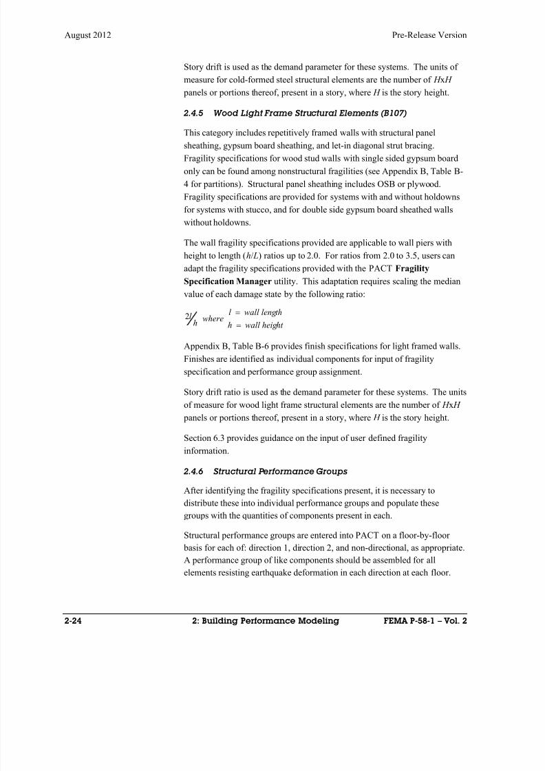
8/12/2019 Seismic Performance Assessment of Buildings
http://slidepdf.com/reader/full/seismic-performance-assessment-of-buildings 52/358
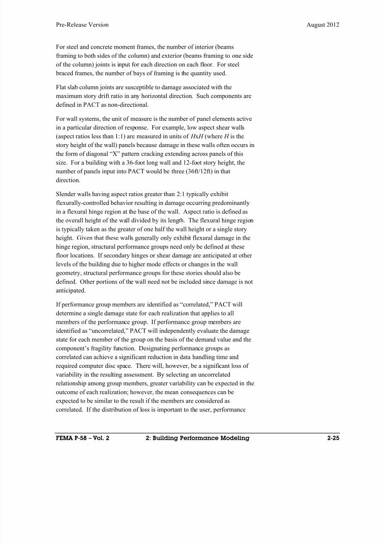
8/12/2019 Seismic Performance Assessment of Buildings
http://slidepdf.com/reader/full/seismic-performance-assessment-of-buildings 53/358
Pre-Release Version August 2012
FEMA P-58 – Vol. 2 2: Building Performance Modeling 2-25
For steel and concrete moment frames, the number of interior (beams
framing to both sides of the column) and exterior (beams framing to one side
of the column) joints is input for each direction on each floor. For steel
braced frames, the number of bays of framing is the quantity used.
Flat slab column joints are susceptible to damage associated with themaximum story drift ratio in any horizontal direction. Such components are
defined in PACT as non-directional.
For wall systems, the unit of measure is the number of panel elements active
in a particular direction of response. For example, low aspect shear walls
(aspect ratios less than 1:1) are measured in units of H x H (where H is the
story height of the wall) panels because damage in these walls often occurs in
the form of diagonal “X” pattern cracking extending across panels of this
size. For a building with a 36-foot long wall and 12-foot story height, the
number of panels input into PACT would be three (36ft/12ft) in that
direction.
Slender walls having aspect ratios greater than 2:1 typically exhibit
flexurally-controlled behavior resulting in damage occurring predominantly
in a flexural hinge region at the base of the wall. Aspect ratio is defined as
the overall height of the wall divided by its length. The flexural hinge region
is typically taken as the greater of one half the wall height or a single story
height. Given that these walls generally only exhibit flexural damage in the
hinge region, structural performance groups need only be defined at these
floor locations. If secondary hinges or shear damage are anticipated at other
levels of the building due to higher mode effects or changes in the wall
geometry, structural performance groups for these stories should also be
defined. Other portions of the wall need not be included since damage is not
anticipated.
If performance group members are identified as “correlated,” PACT will
determine a single damage state for each realization that applies to all
members of the performance group. If performance group members are
identified as “uncorrelated,” PACT will independently evaluate the damage
state for each member of the group on the basis of the demand value and the
component’s fragility function. Designating performance groups as
correlated can achieve a significant reduction in data handling time andrequired computer disc space. There will, however, be a significant loss of
variability in the resulting assessment. By selecting an uncorrelated
relationship among group members, greater variability can be expected in the
outcome of each realization; however, the mean consequences can be
expected to be similar to the result if the members are considered as
correlated. If the distribution of loss is important to the user, performance
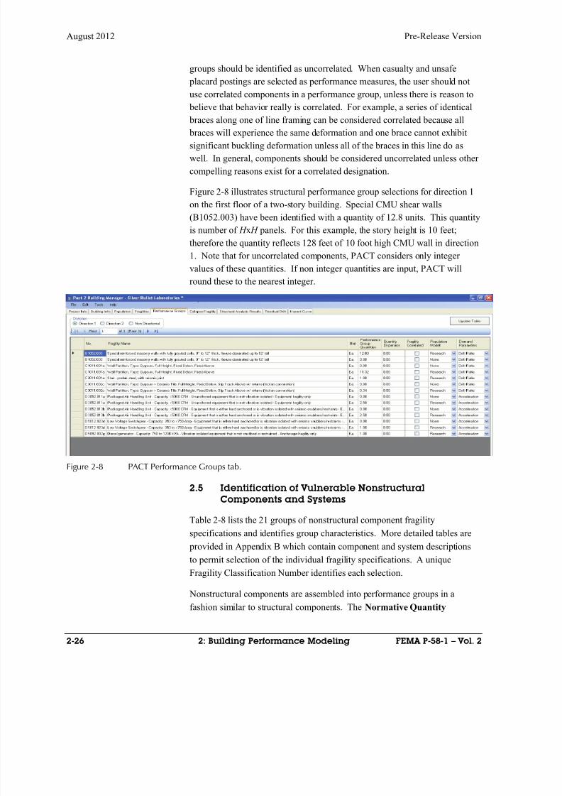
8/12/2019 Seismic Performance Assessment of Buildings
http://slidepdf.com/reader/full/seismic-performance-assessment-of-buildings 54/358
August 2012 Pre-Release Version
2-26 2: Building Performance Modeling FEMA P-58-1 – Vol. 2
groups should be identified as uncorrelated. When casualty and unsafe
placard postings are selected as performance measures, the user should not
use correlated components in a performance group, unless there is reason to
believe that behavior really is correlated. For example, a series of identical
braces along one of line framing can be considered correlated because all
braces will experience the same deformation and one brace cannot exhibit
significant buckling deformation unless all of the braces in this line do as
well. In general, components should be considered uncorrelated unless other
compelling reasons exist for a correlated designation.
Figure 2-8 illustrates structural performance group selections for direction 1
on the first floor of a two-story building. Special CMU shear walls
(B1052.003) have been identified with a quantity of 12.8 units. This quantity
is number of H x H panels. For this example, the story height is 10 feet;
therefore the quantity reflects 128 feet of 10 foot high CMU wall in direction
1. Note that for uncorrelated components, PACT considers only integer
values of these quantities. If non integer quantities are input, PACT will
round these to the nearest integer.
Figure 2-8 PACT Performance Groups tab.
2.5 Identification of Vulnerable Nonstructural
Components and Systems
Table 2-8 lists the 21 groups of nonstructural component fragilityspecifications and identifies group characteristics. More detailed tables are
provided in Appendix B which contain component and system descriptions
to permit selection of the individual fragility specifications. A unique
Fragility Classification Number identifies each selection.
Nonstructural components are assembled into performance groups in a
fashion similar to structural components. The Normative Quantity

8/12/2019 Seismic Performance Assessment of Buildings
http://slidepdf.com/reader/full/seismic-performance-assessment-of-buildings 55/358
Pre-Release Version August 2012
FEMA P-58 – Vol. 2 2: Building Performance Modeling 2-27
Table 2-8 Summary of Provided Nonstructural Component and System Fragility Specifications
Fragility Specification Name Items IncludedRange of Fragility Classification
Numbers
B201: Exterior Nonstructural Walls Precast Panels, Masonry Parapets B2010.201, B2010,201b, B2012.001a
B202: Exterior Window Systems Exterior Curtain Wall and Storefront MetalFramed Window Systems
B2022.001 – 201
B2023.001 - 058B30: Roof Elements Roof Tile, Masonry Chimney B3011.011-014, B3031.001a-002c
C101: Partitions (nonstructural) GWB with taped/painted finish B1011.001a-011b
C201: Stairs Prefab Steel & Concrete, Cast-in-Place, hybrid C2011.001a – C2011.031b
C301: Wall Finishes Wall Paper, Ceramic Tile, High End (marble orwood)
C3011.001a – C3011.003c
C302: Floor Finishes, Raised AccessFloors and Floor Flooding
Raised Access Floors, Floor Flooding C3027.001 - C3021.001p
C303: Ceilings and Ceiling Lighting Suspended Ceilings, Embedded Ceiling Lightingand Pendant Lighting Systems
C3032.001a – C3032.004d
C3033.001-2, C3034.001-2
D10: Conveying Elevators (traction , hydraulic) D1014.011, D1014.012 D1014.021,D1041.022
D202: Domestic Cold/Hot Water Piping Threaded steel, welded steel D2021.011a – D2021.014bD2022.011a - D2022.014b
D203 Sanitary Waster Piping Cast Iron D2031.011b – D2031.024b
D205: Chilled Water Steam Piping Welded, Threaded D2051.011a-
D2051.024b
D206: Steam Piping Welded, Threaded D2061.011 - D2061.024a
D303: Chillers, Cooling Towers andCompressors
Unanchored, isolated (restrained andunrestrained) Anchored
D3031.011a – D3031.023l
D3032.011a – D3032.013l
D304: HVAC Distribution Systems Fans, In-Line Fanes, Ducting, Drops/Diffusers,VAV Boxes
D3031.101a – D3041.103c
D3041.001a – D3041.041b
D305: Packaged Air Handling Units Unanchored, Isolated (restrained) anchored D3052.011a – D3052.013l
D40: Fire Sprinklers Old Style Victaulic Systems, Standard ThreadedDrops D4011.011a – D4011.074a
D501: Motor Control Centers,Transformers, LV Switchgear,Distribution Panels
Unanchored, isolated (restrained) anchored D5010.011a – D5012.033l
D509: Other Electrical Battery Rack, Battery Charger, Generator D5092.011a – D5092.033l
E20: Equipment and Furnishings Home Entertainment Systems, ElectronicEquipment, desktop electronics, fragile objects,Modular workstations, Bookcases, Filing Cabinets
E2022.020 – E2022.125b
F20: Special Construction Steel Storage Racks F1012.001
Estimation tool is provided in Volume 3 to facilitate identification of typical
quantity and distribution of common nonstructural building components based on occupancy. To use this tool, users identify the floor area associated
with each of 8 different occupancies at each building level. The workbook
produces a level by level list of the typical quantities of ceiling, light fixtures,
cladding, fire sprinkler lines and other components. These quantities are
identified using the typical quantities of these components per square foot,
per occupancy factored by the square footage of that occupancy actually
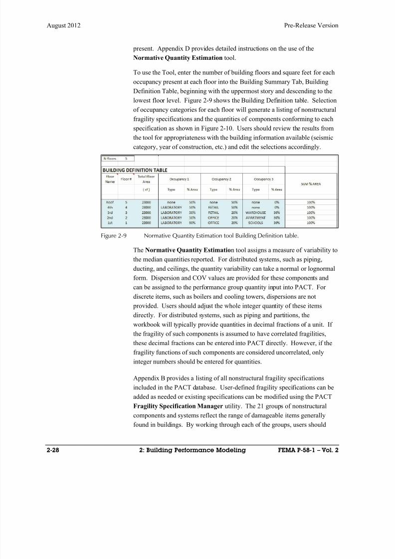
8/12/2019 Seismic Performance Assessment of Buildings
http://slidepdf.com/reader/full/seismic-performance-assessment-of-buildings 56/358
August 2012 Pre-Release Version
2-28 2: Building Performance Modeling FEMA P-58-1 – Vol. 2
present. Appendix D provides detailed instructions on the use of the
Normative Quantity Estimation tool.
To use the Tool, enter the number of building floors and square feet for each
occupancy present at each floor into the Building Summary Tab, Building
Definition Table, beginning with the uppermost story and descending to thelowest floor level. Figure 2-9 shows the Building Definition table. Selection
of occupancy categories for each floor will generate a listing of nonstructural
fragility specifications and the quantities of components conforming to each
specification as shown in Figure 2-10. Users should review the results from
the tool for appropriateness with the building information available (seismic
category, year of construction, etc.) and edit the selections accordingly.
Figure 2-9 Normative Quantity Estimation tool Building Definition table.
The Normative Quantity Estimation tool assigns a measure of variability to
the median quantities reported. For distributed systems, such as piping,
ducting, and ceilings, the quantity variability can take a normal or lognormal
form. Dispersion and COV values are provided for these components and
can be assigned to the performance group quantity input into PACT. For
discrete items, such as boilers and cooling towers, dispersions are not
provided. Users should adjust the whole integer quantity of these items
directly. For distributed systems, such as piping and partitions, the
workbook will typically provide quantities in decimal fractions of a unit. If
the fragility of such components is assumed to have correlated fragilities,
these decimal fractions can be entered into PACT directly. However, if the
fragility functions of such components are considered uncorrelated, only
integer numbers should be entered for quantities.
Appendix B provides a listing of all nonstructural fragility specifications
included in the PACT database. User-defined fragility specifications can be
added as needed or existing specifications can be modified using the PACT
Fragility Specification Manager utility. The 21 groups of nonstructural
components and systems reflect the range of damageable items generally
found in buildings. By working through each of the groups, users should

8/12/2019 Seismic Performance Assessment of Buildings
http://slidepdf.com/reader/full/seismic-performance-assessment-of-buildings 57/358
Pre-Release Version August 2012
FEMA P-58 – Vol. 2 2: Building Performance Modeling 2-29
trace an organized path that will comprehensively define the damageable
nonstructural building components and systems.
Figure 2-10 Normative Quantity Estimation tool Component Summary Matrix.
There are many items not included in the PACT database that may be
damaged when subjected to ground shaking. Users can develop fragility
functions for these items. Volume 1 Section 3.8 provides guidance on this
topic which is further illustrated in Chapter 7.
The following section discusses the 21 general categories of nonstructural
components included.
2.5.1 Exterior Nonstructural Walls (B201)
There are many types of exterior nonstructural walls. Damageability is often
a function of detailing. PACT provides fragility specifications for precast
concrete cladding panels where the user must define the median demand and
dispersion values associated with the damage states. Chapter 7 provides
guidance on development of nonstructural component fragility parameters by
calculation and Chapter 8 for development of consequence functions.
2.5.1.1 Perimeter Cladding Systems
Fragility and consequence functions for these systems should include
consideration of the size of the gap provided in the panel system to
accommodate horizontal drift. The in-plane distortion required to bring
adjacent panels into contact can be converted to an equivalent story drift
using the geometry of the panel. Contact points can occur at the panel
corners and at the interface with column cover panels. System suppliers
often can indicate the amount of drift that can be accommodated before
adjacent panels contact. Table 2-9 provides guidance for commonly
constructed gaps as a function of building category and the operative design
code for the period of construction. The table expresses the gap in terms of
8/12/2019 Seismic Performance Assessment of Buildings
http://slidepdf.com/reader/full/seismic-performance-assessment-of-buildings 58/358
August 2012 Pre-Release Version
2-30 2: Building Performance Modeling FEMA P-58-1 – Vol. 2
story drift ratio. Cladding fragility specifications should be adjusted for the
gap provided by adding the story drift accommodation value to the median
demand value of the fragility.
Table 2-9 Suggested Drift Accommodation Ratio a for Precast Concrete Cladding and Other
Brittle Cladding Systems
Building Code Building Occupancy Category per ASCE/SEI 7
I III IV
1994 UBC (ICC, 1994) or before 0.012 0.012 0.012
1997 UBC (ICC, 1997) 0.020 0.020 0.020
2000 IBC (ICC, 2000) – 2009 IBC (ICC, 2009) 0.020 0.015 0.010
2012 IBC (ICC, 2012) or thereafter 0.020 0.019 0.015
In-plane story drift ratio is the demand parameter for cladding systems. The
area of cladding per floor is dependent on the floor perimeter in eachdirection and the height of the floor (less the area of glazing). Quantity units
are the net cladding area (in square feet) in each direction between floors
divided by 1000.
Perimeter cladding systems may also be vulnerable to damage when out of
plane floor accelerations or drifts exceed the component or anchorage
capacity. To avoid double counting damage to the same component, only the
specification for the governing demand should be input to the assessment
model. In cases where vulnerability to in-plane and out-of-plane demands is
comparable, some of the components can be assigned to one performance
group, having in-plane vulnerability, and the balance to a second group
having out-of-plane vulnerability.
2.5.1.2 Precast Concrete Cladding Panels
Two fragility specifications are provided for precast concrete cladding
panels. One is associated with damage in-plane while the other fragility is
associated with out-of-plane damage. Users must provide the median demand
and dispersion values based on the details of the system present.
Unless panel detailing indicates greater capacity, it is suggested that the
median in-plane demand requiring panel replacement be taken as (δa + 0.005)
where a is the required code drift accommodation as indicated in Table 2-9.
A dispersion value of 0.50 is suggested.
Peak floor acceleration in the direction normal to the wall at the top floor
adjacent to a panel is the demand parameter used for out-of-plane damage.
Section 7.3 provides guidance on the calculation of anchorage fragilities. For
8/12/2019 Seismic Performance Assessment of Buildings
http://slidepdf.com/reader/full/seismic-performance-assessment-of-buildings 59/358
Pre-Release Version August 2012
FEMA P-58 – Vol. 2 2: Building Performance Modeling 2-31
most situations, a crude but adequate calculation can be made by using the
code seismic design acceleration coefficient for which the anchorage was
presumed to be designed (see Section 7.3.1) and converting this to a median
estimate of capacity.
Failure of precast concrete cladding has no life safety consequences withinPACT because the exterior population model is unknown.
2.5.1.3 Masonry Parapets
PACT fragility specifications are provided for unreinforced, unbraced
masonry parapets. The demand parameter is peak roof acceleration normal
to the parapet wall. The performance group quantity units are 100 linear feet
of wall. As with precast cladding, failure of masonry parapets does not have
any life safety consequences in PACT, although real consequences can exist.
2.5.2 Exterior Window Systems (B202)
Table B202 lists exterior window systems fragility specifications. The
specifications are based on testing of modern metal framed exterior window
systems. The testing was performed on glazing with square cut corners (the
most common form of exterior window construction). A total of 48 fragility
specifications are provided. Forty-four of these fragilities reflect specific
glazing installation details while four are provided for situations when the
glazing installation detail is not defined and represents a composite of all
possible details.
Fragility data for two basic window system types are provided: curtain wallsystems and storefront systems. Both are for window systems supported and
contained within aluminum framing. Twenty-eight of the fragility
specifications are for site-built curtain wall systems, which is the most
common form of construction in the commercial building industry and for
which most testing has been performed. One specification is provided for
unitized curtain wall and 15 specifications for storefront window systems.
The site-built curtain wall system specifications are divided into 6
configuration types: monolithic (single pane), symmetric (dual pane with
equal thicknesses), insulated glazing units (IGU), asymmetric (dual pane
with unequal thicknesses) IGUs, and laminated versions of each of these.These system types are further subdivided into three types of glass: annealed,
heat-strengthened and fully-tempered. Separate specifications are provided
for variations in glazing edge clearances, glazing aspect ratios, and glass
thicknesses.

8/12/2019 Seismic Performance Assessment of Buildings
http://slidepdf.com/reader/full/seismic-performance-assessment-of-buildings 60/358
August 2012 Pre-Release Version
2-32 2: Building Performance Modeling FEMA P-58-1 – Vol. 2
The storefront window system specifications are also subdivided into
configuration types including: monolithic, symmetric, and asymmetric IGUs
with laminated glass for some selections, with further subdividision into
annealed and fully tempered glass types. Separate specifications recognize
variations in glazing edge clearances, glazing aspect ratios and glass
thicknesses.
Particularly for existing buildings, in many situations, the details of glazing
installation may not be known. Six additional fragility specifications have
been provided for these situations. Four of these are for curtain wall window
systems and two are for storefront window systems. The curtain wall
specifications are divided into two configuration types: monolithic and IGU
glazing. There is no subdivision for laminated glazing. It is assumed that the
glazing aspect ratio is 6:5. The glazing edge clearance and glass thicknesses
are assumed as unknown and variations are incorporated into the provided
specifications.
The fragility information provided is based on the size of glazing panels
tested. The median drifts associated with the damage states should be
adjusted if smaller or larger glazing panels are used and the gap clearances
are basically the same as those for which fragilities are provided. The
adjustment factor is the ratio of the tested panel height divided by actual
panel height. This ratio is multiplied by the median drift value for each
damage state in the specification. Table 2-10 lists the heights of tested
panels for each aspect ratio.
Where specific knowledge or details of the exterior window system is
unavailable, it is suggested to use the IGU specifications with a 6:5 aspect
ratio for curtain wall applications, and the monolithic fragility specifications
for storefront applications.
Table 2-10 Tested Window Pane Sizes
Aspect Ratio Tested Panel Height
6:5 6 feet
2:1 8 feet
1:2 4 feet
Metal panels are frequently used in conjunction with exterior window
systems. Generally, the exterior window system will exhibit damage before
the metal-panel system. The fragility functions for the window system can
be used for the combined system and the user can modify the consequence
function in PACT to reflect the consequences to the entire system. See
Chapter 8 for guidance on modifying consequence functions.

8/12/2019 Seismic Performance Assessment of Buildings
http://slidepdf.com/reader/full/seismic-performance-assessment-of-buildings 61/358
Pre-Release Version August 2012
FEMA P-58 – Vol. 2 2: Building Performance Modeling 2-33
The demand parameter for exterior windows is the story drift ratio in the
plane of the wall. The area of glazing per floor is dependent on the perimeter
length of the floor in the direction under consideration and height of the floor
less the area of perimeter cladding or other non-glazed areas. The quantity
units for performance group input is the net window area (in square feet) for
the floor divided by 1000.
2.5.3 Roof Elements (B30)
2.5.3.1 Roof Coverings (B301)
Two sets of fragility specifications are provided for sloping tile roofs:
concrete tiles and clay tiles. The specifications are further defined depending
on whether attachment to the structure is compliant with the requirements of
the 1994UBC, Uniform Building Code (ICC, 1994), and later codes or not.
The demand parameter for these specifications is peak roof acceleration
(non-directional). The performance group quantity units is the tiled roof area(increased for slope) in square feet divided by 100 (gsf).
2.5.3.2 Unreinforced Masonry Non-Industrial Chimneys
(B303)
PACT fragility specifications are provided for unreinforced non-industrial
masonry chimneys. The specifications are subdivided by chimney height
above the roof, including: 5 feet, 10 feet and 15 feet. Each of these
categories is further subdivided into two selections that include
reconstruction of the chimney with reinforced masonry or replacement with a
framed alternative. Most jurisdictions no longer permit these types ofchimneys in areas of significant seismic risk. Peak roof acceleration (non-
directional) is the demand parameter used in these specifications. The
performance group quantity unit is the number of chimneys.
2.5.4 Partitions (C101)
Table B-4 lists fragility specifications for gypsum wall board partitions on
metal and wood studs (fragility classification number C101). Paint finish
and taped joints are assumed. Table B-6 lists other available wall finishes
(fragility classification number C301).
Four subcategories of gypsum wall board partitions on metal studs are
provided: (1) full-height partitions fixed to the underside of the floor at their
top; (2) partial-height partitions sheathed with gypsum wall board 9 feet
vertically and braced to the underside of the above floor; (3) full-height
partitions without corners, slip track top connection restrains out of plane
movement but not in plane horizontal or vertical movement; and (4) full-
8/12/2019 Seismic Performance Assessment of Buildings
http://slidepdf.com/reader/full/seismic-performance-assessment-of-buildings 62/358
August 2012 Pre-Release Version
2-34 2: Building Performance Modeling FEMA P-58-1 – Vol. 2
height partitions with “slip track” connections at their tops and returns at
their ends (corners). The fragility and consequence functions for all four
partition types assume gypsum wall board on both sides of the partition and
include allowances for all typical accessories including: doors and embedded
mechanical and electrical utilities. For damage states where the consequence
includes partition replacement, the repair cost includes allowance for these
accessories.
Two subcategories of wood stud partitions are provided: full-height partitions
fixed to the underside of the floor at their top, and partial-height partitions
sheathed with gypsum board for 9 feet and braced to the underside of the
floor above. The fragility and consequence functions for both types of
partitions assume gypsum wall board on both sides and include allowances
for all typical accessories including doors and embedded mechanical and
electrical utilities. For damage states where the consequence includes
partition replacement, the repair costs include allowance for theseaccessories.
Wall finishes on partitions, other than a painted finish with taped joints, are
addressed separately. It is assumed that partitions will be constructed the
same regardless of finish type and will include a painted finish with taped
joints. The partition fragility specifications in Table B-4 must be separately
included as partition walls. Section 2.5.6 lists the available wall finish
fragility specifications. These specifications assume the wall finish is
applied to one side of the wall only. This permits different wall finishes to
be specified for opposite sides of the same wall.
Story drift ratio in the plane of the wall is the demand parameter used with
these specifications. The performance group quantity is linear feet of wall
divided by 200. For purposes of estimating repair costs it is assumed walls
are 9 feet tall.
2.5.5 Stairs (C201)
Four types of interior egress stair fragility specifications are provided: (1)
prefabricated steel stair assemblies; (2) prefabricated precast concrete stair
assemblies; (3) cast-in-place concrete stairs; and (4) hybrid stairs (steel stairstringers with precast concrete treads). Cast-in-place concrete stairs placed
monolithically with the structure should be included in the structural analysis
model. Stair specifications are further subdivided based on support condition
including: stairs fixed at both ends and stairs with bottom ends having slotted
joints designed to accommodate story drift. For existing buildings, if the
8/12/2019 Seismic Performance Assessment of Buildings
http://slidepdf.com/reader/full/seismic-performance-assessment-of-buildings 63/358
Pre-Release Version August 2012
FEMA P-58 – Vol. 2 2: Building Performance Modeling 2-35
details of stair installation are not available, it is reasonable to assume the
stairs are a hybrid type without slotted joints, i.e., fixed at both ends.
Consequence functions are provided for all stair types. Fragility functions
are only provided for prefabricated stair assemblies (steel, precast, hybrid)
composed of individual stringers, stair treads and landings assembled withoutseismic joints. Fragility functions are not provided for cast-in-place and
monolithic precast stairs. These components require user input fragility
functions. Chapter 6 and Chapter 7 provide guidance on developing fragility
functions by calculation.
Fragility functions for stairs with seismic joints are specified by the user. A
suggested approach for establishing a fragility function for this condition
requires estimating the story drift the joint is designed to accommodate and
adding that drift to the drift in the PACT database for the component without
a seismic joint.
Story drift ratio in the direction of stair alignment is the demand parameter
for these specifications. If the directional orientation of the stair is unknown,
the demand parameter can be adjusted to non-directional. The number of
stairs is based on gross square foot of building floor area and occupancy.
Volume 1 Appendix F provides quantity guidance for stairways per floor
based on gross square foot of building floor area and occupancy. For
buildings that have the same floor area at all floors, the same number of stairs
should be specified at each level. The performance group quantity measure
is stairways per floor.
2.5.6 Wall Finishes (C301)
Three fragility specifications are provided for wall finishes other than paint:
wall paper, ceramic tile, and high end finish including marble or wood
paneling. These fragility specifications are further subdivided depending on
whether the finishes are applied to partitions that are: (1) full height and fixed
at the top; (2) partial height and lateral braced at the top, or (3) full height
with “slip track” top connections. The fragility and consequence functions
assume the finish occurs on one side of the partition only. Note that only
damage states and consequences associated with damage to the finishesthemselves are considered in these fragility specifications. The partitions
themselves and these finishes must be input separately.
The quantity of partition finish is based on linear feet of wall, as previously
described for interior partitions. Users must define these independently. If
both sides of a wall have finishes, increase the quantities accordingly.
8/12/2019 Seismic Performance Assessment of Buildings
http://slidepdf.com/reader/full/seismic-performance-assessment-of-buildings 64/358
August 2012 Pre-Release Version
2-36 2: Building Performance Modeling FEMA P-58-1 – Vol. 2
2.5.7 Floor Finishes, Raised Access Floors and Floor Flooding
(C302)
2.5.7.1 Raised Access Floors
Non-directional peak floor acceleration is the demand parameter for raised
access floors.
Two types of fragilities are provided: unanchored floors, including floors
with adhesive attachment, and seismically-rated access floors with pedestals
anchored and braced to the floor. Current seismic codes strongly encourage
seismically-rated floors for buildings assigned to Seismic Design Category
D, E, or F. However, anchorage conditions vary considerably.
The quantity unit for raised access floors is the square footage of floor area
divided by 200.
2.5.7.2 Floor Flooding
A fragility specification is provided to account for floor flooding as a result
of fire sprinkler or pipe leakage. It includes 16 selections. Flooding fragility
specifications are provided for each of the 8 occupancies. These
specifications are further subdivided based on a high or low likelihood of
mold developing subsequent to the flooding. Generally, it is highly likely for
the development of mold in geographic locations in areas of high humidity.
The median demand for floor flooding is user selected as equal to the lowest
median value of a piping component damage state included in the
performance model that will result in a major leak. For Seismic Design
Categories A, B, and C (no ceiling bracing) sprinkler drops will typically
govern the demand selection. For Seismic Design Categories D, E, and F the
demand selection is likely governed by threaded water piping. Flooding
damage is presumed to occur on only the floor where the major leak occurs.
The demand parameters and input quantities are the same as the values for
the piping component with the lowest median damage state demand. For
floor flooding consequences, the default assumption is that the entire floor is
flooded. The user has the option to override the default assumption and
assume only a part of floor is flooded by modifying the consequence function
in the fragility specification. The likelihood of floor flooding throughout a
floor level is related to the presence of building maintenance personnel,
capable of rapidly shutting down sprinkler flow.
2.5.8 Suspended Ceilings and Ceiling Lighting (C303)
Four types of suspended lay-in ceiling specifications are provided based on
conformance to the prescriptive seismic detailing requirements of recent
building codes. Types included are ceilings satisfying detailing requirements
8/12/2019 Seismic Performance Assessment of Buildings
http://slidepdf.com/reader/full/seismic-performance-assessment-of-buildings 65/358
8/12/2019 Seismic Performance Assessment of Buildings
http://slidepdf.com/reader/full/seismic-performance-assessment-of-buildings 66/358
8/12/2019 Seismic Performance Assessment of Buildings
http://slidepdf.com/reader/full/seismic-performance-assessment-of-buildings 67/358
Pre-Release Version August 2012
FEMA P-58 – Vol. 2 2: Building Performance Modeling 2-39
For recently constructed buildings, if the type of distribution system detailing
is not known, select the type appropriate to the building’s Seismic Design
Category and nonstructural importance. For construction that predates the
adoption of codes with seismic detailing for these systems, assume Seismic
Design Category A.
Peak floor acceleration (non-directional) in the floor above is used as the
demand parameter for these specifications. Performance group quantities are
measured in the number of 1000 linear feet units of length per floor.
As previously discussed in Section 2.5.7, it is possible to include a floor
flooding fragility specification to account for flooding damage.
2.5.11 Sanitary Waste Piping (D203)
Table B-11 provides fragility specifications for sanitary waste piping. These
specifications are further divided into subgroups depending on SeismicDesign Category and nonstructural Importance Factor similar to other piping
types. Further subdivision is made for cast iron piping with flexible
couplings and those with ball and spigot couplings. For ball and spigot
couplings separate specifications are provided for the piping and, in most
cases, its anchorage and bracing. Both specifications should be included in
the performance model for these components.
Peak floor acceleration (non-directional) in the floor above is used as the
demand parameter for these specifications. Performance group quantities are
measured in the number of 1000 linear feet units of length per floor.
As with other piping types, it is possible to assign a fragility specification to
account for floor flooding.
2.5.12 Chilled Water and Steam Piping (D205 and D206)
Table B-12 and Table B-13 provide fragility specifications for chilled water
and steam piping. These specifications are further divided into subgroups
depending on Seismic Design Category and nonstructural Importance Further
subdivision is made for welded and threaded connections and for pipe
diameters greater than 2.5 inches and less than 2.5 inches. Separate
specifications are provided for both the piping itself and for anchorage and
bracing supporting the piping. For these components, both specifications
should be specified.
If it is not known what type of distribution detailing exists in a recently
constructed building use the building Seismic Design Category and
nonstructural Importance Factor in accordance with the currently applicable

8/12/2019 Seismic Performance Assessment of Buildings
http://slidepdf.com/reader/full/seismic-performance-assessment-of-buildings 68/358
August 2012 Pre-Release Version
2-40 2: Building Performance Modeling FEMA P-58-1 – Vol. 2
building code. For construction that predates the adoption of codes with
seismic detailing for these systems, assume Seismic Design Category A.
Peak floor acceleration (non-directional) in the floor above is used as the
demand parameter for these specifications. Performance group quantities are
measured in the number of 1000 linear feet units of length per floor.
2.5.13 Chillers, Cooling Towers, Compressors (D303)
Table B-14 provides fragility specifications for chillers, cooling towers and
compressors. Each of these specifications is further subdivided by the
installation characteristics including: unanchored and not isolated; isolated
and not restrained; hard anchored or isolated and restrained. Each of these
subcategories is further subdivided by unit size (less than 100 ton, 100 ton to
350 ton, etc.) or by whether the unit services small or large medical systems
(large and small are general terms subject to user judgment).
The final category used to differentiate among fragility specifications for
these components is the dominant damage mode. Three possible damage
modes are identified. These include:
Anchorage failure: Equipment anchorage is relatively weak and fails
well before the equipment is damaged
Internal Damage: Equipment anchorage is relatively strong and the
equipment suffers internal damage well before the anchorage fails
Simultaneous Anchorage Failure and Internal Damage: Equipment
anchorage fails and is accompanied by internal damage to the equipment.
Consequence functions are provided for each of these fragility specifications;
however, users are required to define the median acceleration value
associated with anchorage failure for each piece of equipment. With this
calculated value, the Fragility Specification Manager utility can determine
the best selection for the dominant damage mode by comparing median floor
accelerations for the anchorage and the equipment damage modes (PACT
fragility selections for the equipment damage mode include median floor
acceleration values and dispersion values). Users should:
Select the anchorage failure damage mode if the median value of peak
floor acceleration associated with anchorage failure is less than 30% of
the value associated with internal damage to the equipment.
Select the equipment internal damage mode if the median peak floor
acceleration for internal equipment damage is less than 30% of the
median value of acceleration associated with anchorage failure.
8/12/2019 Seismic Performance Assessment of Buildings
http://slidepdf.com/reader/full/seismic-performance-assessment-of-buildings 69/358
Pre-Release Version August 2012
FEMA P-58 – Vol. 2 2: Building Performance Modeling 2-41
For all other median acceleration ratios, select the simultaneous
anchorage failure and internal equipment damage mode.
For equipment that is unanchored, only damage modes that include internal
damage are provided in PACT. Users can define additional damage modes
associated with failure of attached piping due to equipment sliding. Section7.3 provides guidance on calculation of anchorage fragilities.
Non-directional peak floor acceleration is used as the demand parameter for
these specifications. Estimates of the size and number of equipment items
likely to occur given the size and occupancy of the building under
construction can be found in Volume 1 Appendix F and the Normative
Quantity Estimation tool. The capacity of an individual equipment item is
expressed in terms of the gross square footage of building area it can serve.
Depending on the total demand, the size and number of equipment units can
be assigned. If the demand exceeds the capacity of any available unit(greater than 1,000 ton), assign two items of equipment equal in size that
provide the needed total capacity. Most equipment identified in this table
will be located on the first floor, basement or roof. Items should only be
identified once for a given building.
2.5.14 HVAC Distribution Systems (D304)
Table B-15 provides fragility specifications for components of HVAC
distribution systems including: in-line fans, ducting, drops and diffusers,
variable air volume boxes, and fans. In-line fan specifications are divided
into subgroups that include units that are independently supported withvibration isolators and those without vibration isolation. These systems are
further divided depending on Seismic Design Category as follows: (1)
Seismic Design Categories A and B; (2) Seismic Design Category C; (3)
Seismic Design Categories D and E; and (4) Seismic Design Category D, E,
or F.
Distribution ducting is divided into galvanized and stainless steel sheet metal.
These specifications are further subdivided by size (less than 6 square feet in
cross sectional area or greater than 6 feet). Similar to in-line fans, ducting
specifications are further subdivided by Seismic Design Category.
Drop and diffuser specifications are divided into categories that reflect the
installation of independent safety wires. These specifications are further
subdivided by Seismic Design Category.
Variable air volume boxes (VAV) are divided into two categories: Seismic
Design Category A or B and SDC C or above.
8/12/2019 Seismic Performance Assessment of Buildings
http://slidepdf.com/reader/full/seismic-performance-assessment-of-buildings 70/358
August 2012 Pre-Release Version
2-42 2: Building Performance Modeling FEMA P-58-1 – Vol. 2
HVAC fan specifications are divided into 3 categories: unanchored and not
isolated, isolated but not restrained and hard anchored or isolated and
restrained. These 3 categories are further subdivided by dominant damage
mode in a manner similar to that done for the components in Section 2.5.13.
In an analogous fashion, the user must determine the median value of peak
floor acceleration that will produce anchorage or isolator failure and use that
value to select the dominant damage mode most appropriate.
Peak floor acceleration (non-directional) in the floor above is used as the
demand parameter for these specifications. Performance group quantity units
are as follows:
In-Line Fans: Number of 10 units
HVAC ducting: Number of 1,000 linear feet units
Drops/diffusers: Number of 10 units
VAV boxes: Number of 10 units
HVAC fans: Number of items
2.5.15 Control Panels (Table D305)
Table B-16 provides fragility specifications for control panels. Specification
selections are divided into unanchored and anchored panels. For unanchored
systems, only one specification is provided (Internal Damage), however, for
hard anchored panels, the user should select the most appropriate fragility
specification based on a dominant damage mode that includes anchorage
failure, internal equipment damage or the simultaneous occurrence of both.
Section 2.5.13 provides further information on estimating the median floor
acceleration associated with anchorage failure and the use of that information
to select the most appropriate damage mode.
Non-directional peak floor acceleration of the supporting floor is used as the
demand parameter for these specifications. Performance group quantity units
are “each”.
2.5.16 Packaged Air Handling Units (D306)
Table B-17 provides fragility specifications for packaged air handling units.
These specifications are divided into categories for equipment that is
unanchored and not isolated and equipment that is hard anchored or isolated
and restrained. Each of these categories is further subdivided by equipment
size as follows:
Equipment size < 5,000 cfm

8/12/2019 Seismic Performance Assessment of Buildings
http://slidepdf.com/reader/full/seismic-performance-assessment-of-buildings 71/358
Pre-Release Version August 2012
FEMA P-58 – Vol. 2 2: Building Performance Modeling 2-43
5,000 cfm ≤ Equipment Size < 10,000 cfm
10,000 cfm ≤ Equipment Size < 25,000 cfm
25,000 cfm ≤ Equipment Size < 40,000 cfm
Categories are further subdivided by the dominant damage mode (note for
unanchored, non isolated equipment, only an internal damage mode is
provided). These selections include anchorage failure, internal damage or
the simultaneous occurrence of both. See 2.5.13 for further information on
estimating the median floor acceleration associated with anchorage failure
and the use of that information to select the most appropriate damage mode.
Non-directional peak acceleration of the supporting floor is used as the
demand parameter for these specifications. Performance group quantities are
“each.”
2.5.17 Fire Protection (D401)
Table B-18 lists fragility specifications for fire protection system
components. Testing of connections indicate that vertical standpipes
designed and installed in accordance with NFPA 13, Standard for
Installation of Sprinkler Systems (NFPA, 2007), have a median story drift
ratio capacity exceeding 0.05 and are therefore considered seismically
rugged.
Specifications for thin wall piping systems with older Victaulic type
connections are subdivided by Seismic Design Category. The fragility
specifications provided for the horizontal distribution system includes its
bracing. New style Victaulic coupled sprinkler piping systems and those
sprinkler piping systems with threaded piping couplings are deemed rugged.
Fire sprinkler drop fragility specifications are subdivided into the following
categories:
Lay-in tile soft ceilings
Lay-in tile hard ceilings
No ceilings
Each of these groups is further divided based on Seismic Design Category.
Seismic Design Categories A, B, or C imply no seismic requirements or
lateral bracing of the ceiling while Seismic Design Category D, E, and F
imply that lateral seismic bracing is provided with a stringent level of design
and construction installation review.
8/12/2019 Seismic Performance Assessment of Buildings
http://slidepdf.com/reader/full/seismic-performance-assessment-of-buildings 72/358
August 2012 Pre-Release Version
2-44 2: Building Performance Modeling FEMA P-58-1 – Vol. 2
Non-directional peak floor acceleration of the floor above is used as the
demand parameter for these specifications. Performance group quantities for
horizontal piping are measured in the number of 1,000 linear feet units of
length per floor. Performance group units for drops are measured in units of
100.
2.5.18 Motor Control Centers, Transformers, LV Switchgear,
Distribution Panels (D501)
Table B-19 provides fragility specifications for the following building
electrical components:
Motor control centers
Primary service transformers
Low voltage switchgear
Distribution panels
Each of these fragility specifications are sub-divided by the following
considerations:
Unanchored, not isolated
Hard anchored or isolated and restrained
For transformers, further subdivisions are made based on unit size as follows:
<100 kva
100 to 350 kva
350 to 750 kva
750 1,500 kva
For switchgear and distribution panels, the following subdivisions are used:
100 to 350 amp
350 to 750 amp
750 1,200 amp
1,200 2,000 amp
All of the fragility specifications are further divided by the dominant damage
mode (anchorage failure, internal damage and simultaneous occurrence of
both). Section 2.5.13 provides information on estimating the median floor
acceleration associated with anchorage failure and the use of that information
to select the most appropriate damage mode.
8/12/2019 Seismic Performance Assessment of Buildings
http://slidepdf.com/reader/full/seismic-performance-assessment-of-buildings 73/358
Pre-Release Version August 2012
FEMA P-58 – Vol. 2 2: Building Performance Modeling 2-45
Peak floor acceleration (directional) of the supporting floor is used as the
demand parameter for these specifications. Performance group quantities are
“each.”
2.5.19 Other Electrical Systems (D509)
Table B-20 provides fragility specifications for the following building
electrical components not included in Section 2.5.18:
Battery racks
Battery chargers
Diesel generators
Fragility specifications for these items are subdivided into the following
categories:
Unanchored, not isolated
Hard anchored or isolated and restrained
Diesel generators include specifications for conditions where the equipment
is isolated and not restrained as well as the above conditions. Diesel
generator fragility specifications are further subdivided by equipment size
into the following groups:
100 to 350 kva
350 to 750 kva
750 1,200 kva
1,200 2,000 kva
All the fragility specifications in Table D509 are further subdivided by
dominant damage modes that include anchorage failure, internal equipment
damage and the simultaneous occurrence of both.
Refer to Section 2.5.13 for further information on estimating the median
floor acceleration associated with anchorage failure and the use of that
information to select the most appropriate damage mode.
Peak floor acceleration (directional) of the supporting floor is used as thedemand parameter for these specifications. Performance group quantities are
“each.”

8/12/2019 Seismic Performance Assessment of Buildings
http://slidepdf.com/reader/full/seismic-performance-assessment-of-buildings 74/358
8/12/2019 Seismic Performance Assessment of Buildings
http://slidepdf.com/reader/full/seismic-performance-assessment-of-buildings 75/358
Pre-Release Version August 2012
FEMA P-58 – Vol. 2 2: Building Performance Modeling 2-47
Two fragility specifications types are provided for filing cabinets. One type
is for unanchored filing cabinets and the other is for anchored filing cabinets.
The specifications are further sub-divided depending on the size and
orientation of the filing cabinets. Specifications are provided for two sizes
each of vertical and lateral filing cabinets filing cabinets. The demand
parameter for unanchored filing cabinets is peak total floor velocity of the
supporting floor. Fragility specifications for these components have been
derived by calculation. Section 7.2.1 illustrates this calculation.
For anchored filing cabinets, the demand parameter is peak floor acceleration
(non-directional) of the supporting floor. Fragility specifications are user-
defined and can be developed following the guidance in Chapter 7. The user
needs to define the number of filing cabinets of each type on each floor. The
performance group unit of input is the number of file cabinets of each type
per floor.
2.5.21 Special Construction (F20)
One fragility specification is provided for industrial type storage racks
designed and installed to satisfy the seismic design requirements enforced
prior to 2007. Users must identify and input the number of racks and the
replacement cost of the rack contents. The demand parameter used with this
fragility specification is peak floor acceleration (non-directional) of the floor
supporting the rack. The units of performance group input are the number of
storage racks.
2.6 Collapse Fragility Analysis
Once the building performance model has been developed and input into
PACT, a building collapse fragility function must be developed to permit
assessment of casualties. The collapse fragility function expresses the
probability of building collapse, in one or modes, as a function of spectral
acceleration at the first mode period.
Collapse fragility functions include definition of: the median spectral
response acceleration at the building’s effective fundamental period
and a dispersion β associated with collapse; the possible collapse modes
(expressed as a percentage of each floor area impacted by collapse and the
number of stories involved in the collapse); the probability of each collapsemode given that collapse occurs; and the probability of incurring serious
injuries and fatalities in an area of collapse.
Volume 1 Chapter 6 discusses three general approaches to develop collapse
fragility functions. These three approaches include:
Nonlinear response-history analysis
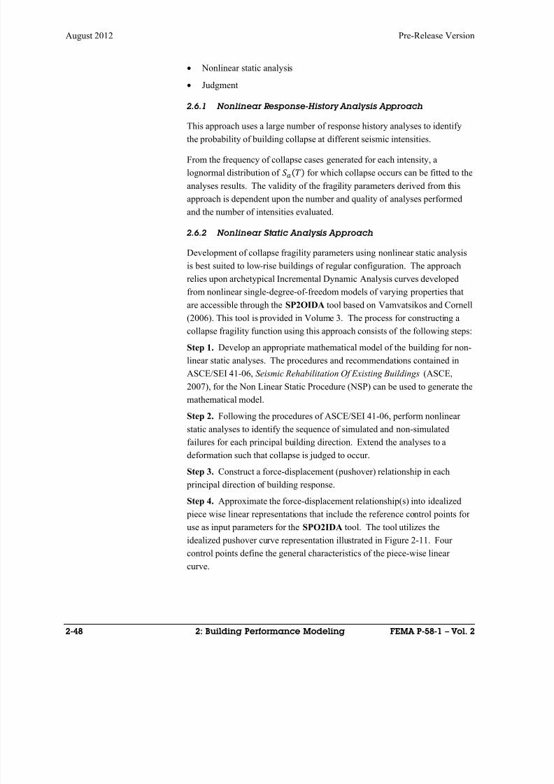
8/12/2019 Seismic Performance Assessment of Buildings
http://slidepdf.com/reader/full/seismic-performance-assessment-of-buildings 76/358
August 2012 Pre-Release Version
2-48 2: Building Performance Modeling FEMA P-58-1 – Vol. 2
Nonlinear static analysis
Judgment
2.6.1 Nonlinear Response-History Analysis Approach
This approach uses a large number of response history analyses to identifythe probability of building collapse at different seismic intensities.
From the frequency of collapse cases generated for each intensity, a
lognormal distribution of for which collapse occurs can be fitted to the
analyses results. The validity of the fragility parameters derived from this
approach is dependent upon the number and quality of analyses performed
and the number of intensities evaluated.
2.6.2 Nonlinear Static Analysis Approach
Development of collapse fragility parameters using nonlinear static analysisis best suited to low-rise buildings of regular configuration. The approach
relies upon archetypical Incremental Dynamic Analysis curves developed
from nonlinear single-degree-of-freedom models of varying properties that
are accessible through the SP2OIDA tool based on Vamvatsikos and Cornell
(2006). This tool is provided in Volume 3. The process for constructing a
collapse fragility function using this approach consists of the following steps:
Step 1. Develop an appropriate mathematical model of the building for non-
linear static analyses. The procedures and recommendations contained in
ASCE/SEI 41-06, Seismic Rehabilitation Of Existing Buildings (ASCE,
2007), for the Non Linear Static Procedure (NSP) can be used to generate themathematical model.
Step 2. Following the procedures of ASCE/SEI 41-06, perform nonlinear
static analyses to identify the sequence of simulated and non-simulated
failures for each principal building direction. Extend the analyses to a
deformation such that collapse is judged to occur.
Step 3. Construct a force-displacement (pushover) relationship in each
principal direction of building response.
Step 4. Approximate the force-displacement relationship(s) into idealized
piece wise linear representations that include the reference control points foruse as input parameters for the SPO2IDA tool. The tool utilizes the
idealized pushover curve representation illustrated in Figure 2-11. Four
control points define the general characteristics of the piece-wise linear
curve.
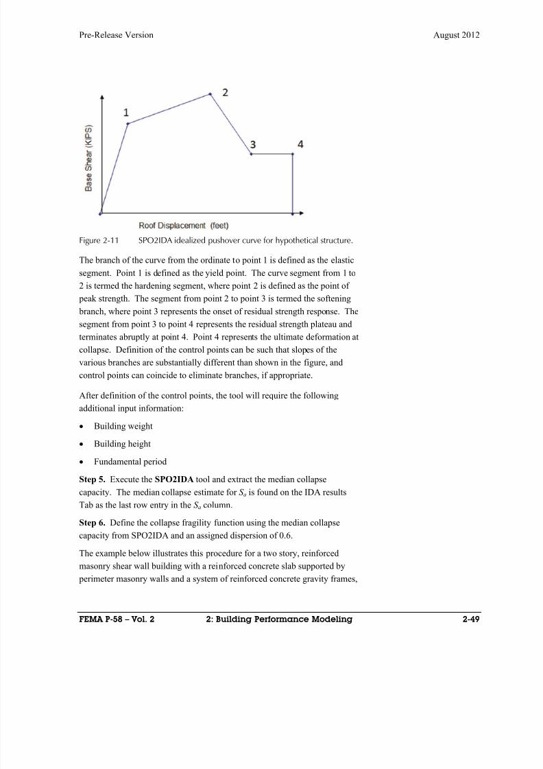
8/12/2019 Seismic Performance Assessment of Buildings
http://slidepdf.com/reader/full/seismic-performance-assessment-of-buildings 77/358
Pre-Release Version August 2012
FEMA P-58 – Vol. 2 2: Building Performance Modeling 2-49
Figure 2-11 SPO2IDA idealized pushover curve for hypothetical structure.
The branch of the curve from the ordinate to point 1 is defined as the elastic
segment. Point 1 is defined as the yield point. The curve segment from 1 to
2 is termed the hardening segment, where point 2 is defined as the point of
peak strength. The segment from point 2 to point 3 is termed the softening
branch, where point 3 represents the onset of residual strength response. The
segment from point 3 to point 4 represents the residual strength plateau and
terminates abruptly at point 4. Point 4 represents the ultimate deformation at
collapse. Definition of the control points can be such that slopes of the
various branches are substantially different than shown in the figure, and
control points can coincide to eliminate branches, if appropriate.
After definition of the control points, the tool will require the following
additional input information:
Building weight
Building height
Fundamental period
Step 5. Execute the SPO2IDA tool and extract the median collapse
capacity. The median collapse estimate for S a is found on the IDA results
Tab as the last row entry in the S a column.
Step 6. Define the collapse fragility function using the median collapse
capacity from SPO2IDA and an assigned dispersion of 0.6.
The example below illustrates this procedure for a two story, reinforced
masonry shear wall building with a reinforced concrete slab supported by
perimeter masonry walls and a system of reinforced concrete gravity frames,
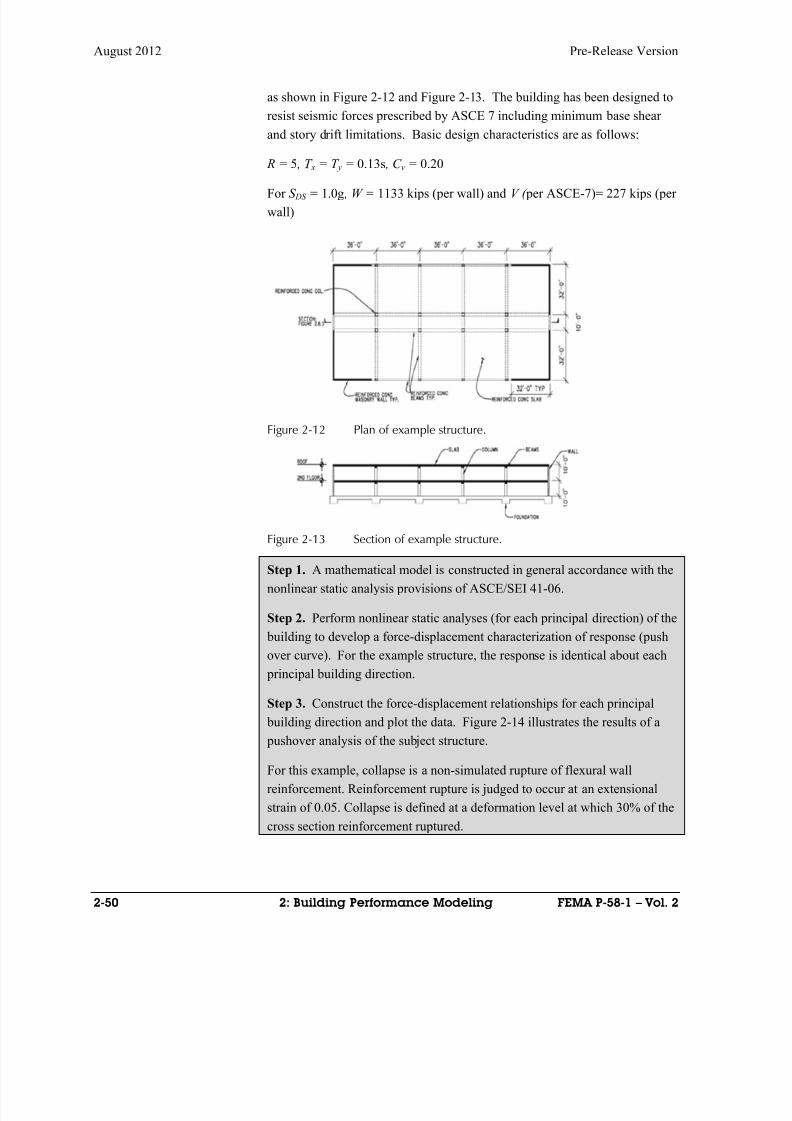
8/12/2019 Seismic Performance Assessment of Buildings
http://slidepdf.com/reader/full/seismic-performance-assessment-of-buildings 78/358
8/12/2019 Seismic Performance Assessment of Buildings
http://slidepdf.com/reader/full/seismic-performance-assessment-of-buildings 79/358
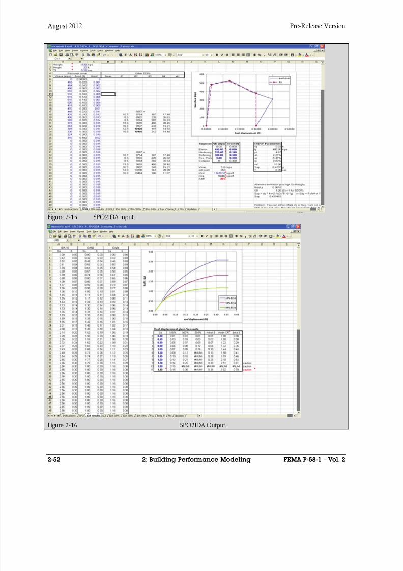
8/12/2019 Seismic Performance Assessment of Buildings
http://slidepdf.com/reader/full/seismic-performance-assessment-of-buildings 80/358
August 2012 Pre-Release Version
2-52 2: Building Performance Modeling FEMA P-58-1 – Vol. 2
Figure 2-15 SPO2IDA Input.
Figure 2-16 SPO2IDA Output.
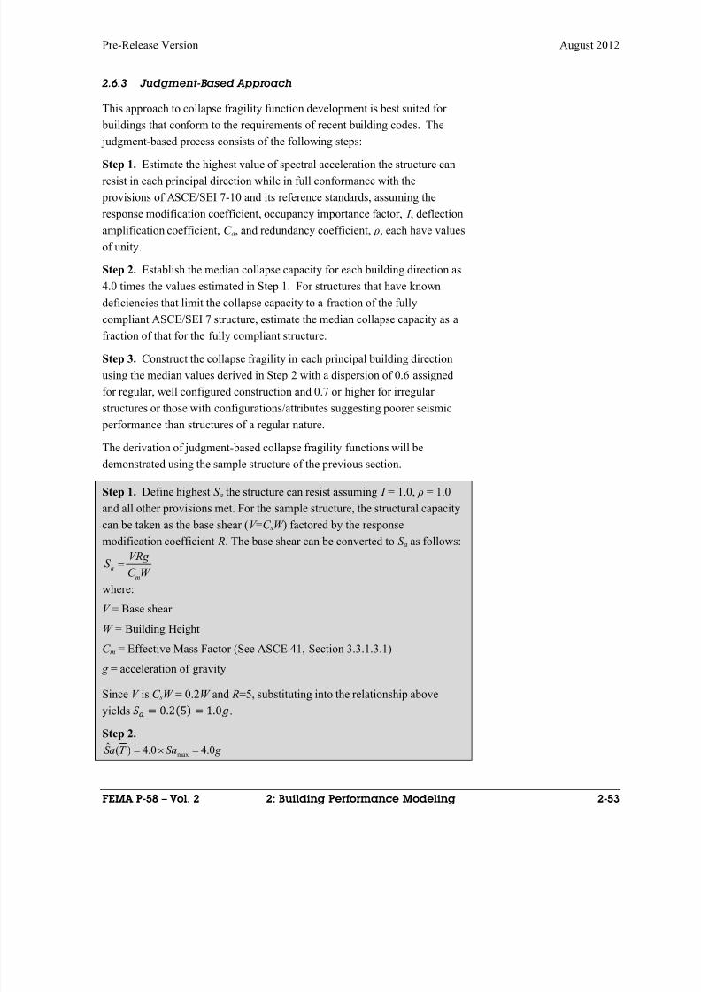
8/12/2019 Seismic Performance Assessment of Buildings
http://slidepdf.com/reader/full/seismic-performance-assessment-of-buildings 81/358
Pre-Release Version August 2012
FEMA P-58 – Vol. 2 2: Building Performance Modeling 2-53
2.6.3 Judgment-Based Approach
This approach to collapse fragility function development is best suited for
buildings that conform to the requirements of recent building codes. The
judgment-based process consists of the following steps:
Step 1. Estimate the highest value of spectral acceleration the structure canresist in each principal direction while in full conformance with the
provisions of ASCE/SEI 7-10 and its reference standards, assuming the
response modification coefficient, occupancy importance factor, I , deflection
amplification coefficient, C d , and redundancy coefficient, ρ, each have values
of unity.
Step 2. Establish the median collapse capacity for each building direction as
4.0 times the values estimated in Step 1. For structures that have known
deficiencies that limit the collapse capacity to a fraction of the fully
compliant ASCE/SEI 7 structure, estimate the median collapse capacity as afraction of that for the fully compliant structure.
Step 3. Construct the collapse fragility in each principal building direction
using the median values derived in Step 2 with a dispersion of 0.6 assigned
for regular, well configured construction and 0.7 or higher for irregular
structures or those with configurations/attributes suggesting poorer seismic
performance than structures of a regular nature.
The derivation of judgment-based collapse fragility functions will be
demonstrated using the sample structure of the previous section.
Step 1. Define highest S a the structure can resist assuming I = 1.0, ρ = 1.0
and all other provisions met. For the sample structure, the structural capacity
can be taken as the base shear (V =C sW ) factored by the response
modification coefficient R. The base shear can be converted to S a as follows:
a
m
VRg S
C W
where:
V = Base shear
W = Building Height
C m = Effective Mass Factor (See ASCE 41, Section 3.3.1.3.1) g = acceleration of gravity
Since V is C sW = 0.2W and R=5, substituting into the relationship above
yields 0.25 1.0.
Step 2.
g SaT aS 0.40.4)(ˆmax
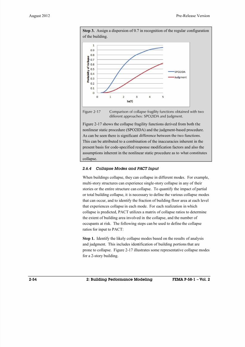
8/12/2019 Seismic Performance Assessment of Buildings
http://slidepdf.com/reader/full/seismic-performance-assessment-of-buildings 82/358
August 2012 Pre-Release Version
2-54 2: Building Performance Modeling FEMA P-58-1 – Vol. 2
Step 3. Assign a dispersion of 0.7 in recognition of the regular configuration
of the building.
Figure 2-17 Comparison of collapse fragility functions obtained with twodifferent approaches: SPO2IDA and Judgment.
Figure 2-17 shows the collapse fragility functions derived from both the
nonlinear static procedure (SPO2IDA) and the judgment-based procedure.
As can be seen there is significant difference between the two functions.
This can be attributed to a combination of the inaccuracies inherent in the
present basis for code-specified response modification factors and also the
assumptions inherent in the nonlinear static procedure as to what constitutes
collapse.
2.6.4 Collapse Modes and PACT Input
When buildings collapse, they can collapse in different modes. For example,
multi-story structures can experience single-story collapse in any of their
stories or the entire structure can collapse. To quantify the impact of partial
or total building collapse, it is necessary to define the various collapse modes
that can occur, and to identify the fraction of building floor area at each level
that experiences collapse in each mode. For each realization in which
collapse is predicted, PACT utilizes a matrix of collapse ratios to determine
the extent of building area involved in the collapse, and the number of
occupants at risk. The following steps can be used to define the collapse
ratios for input to PACT:
Step 1. Identify the likely collapse modes based on the results of analysis
and judgment. This includes identification of building portions that are
prone to collapse. Figure 2-17 illustrates some representative collapse modes
for a 2-story building.
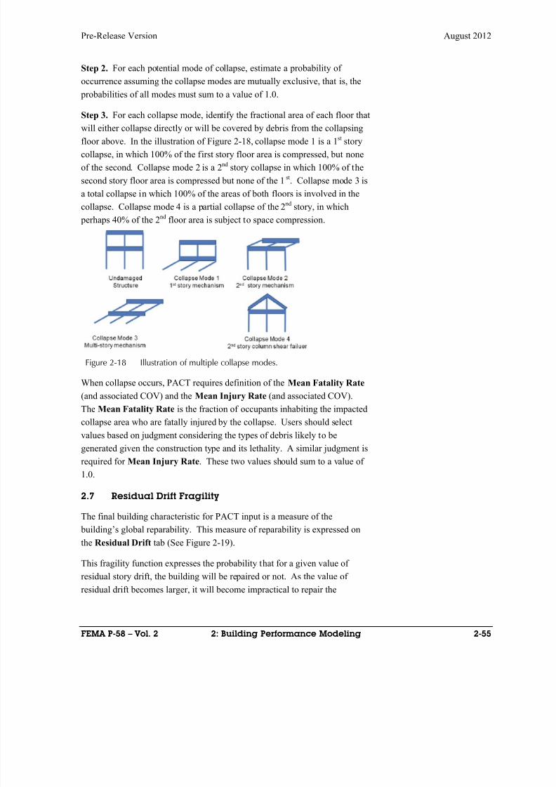
8/12/2019 Seismic Performance Assessment of Buildings
http://slidepdf.com/reader/full/seismic-performance-assessment-of-buildings 83/358
Pre-Release Version August 2012
FEMA P-58 – Vol. 2 2: Building Performance Modeling 2-55
Step 2. For each potential mode of collapse, estimate a probability of
occurrence assuming the collapse modes are mutually exclusive, that is, the
probabilities of all modes must sum to a value of 1.0.
Step 3. For each collapse mode, identify the fractional area of each floor that
will either collapse directly or will be covered by debris from the collapsingfloor above. In the illustration of Figure 2-18, collapse mode 1 is a 1st story
collapse, in which 100% of the first story floor area is compressed, but none
of the second. Collapse mode 2 is a 2nd story collapse in which 100% of the
second story floor area is compressed but none of the 1st. Collapse mode 3 is
a total collapse in which 100% of the areas of both floors is involved in the
collapse. Collapse mode 4 is a partial collapse of the 2nd story, in which
perhaps 40% of the 2nd floor area is subject to space compression.
Figure 2-18 Illustration of multiple collapse modes.
When collapse occurs, PACT requires definition of the Mean Fatality Rate (and associated COV) and the Mean Injury Rate (and associated COV).
The Mean Fatality Rate is the fraction of occupants inhabiting the impacted
collapse area who are fatally injured by the collapse. Users should select
values based on judgment considering the types of debris likely to be
generated given the construction type and its lethality. A similar judgment is
required for Mean Injury Rate. These two values should sum to a value of
1.0.
2.7 Residual Drift Fragility
The final building characteristic for PACT input is a measure of the building’s global reparability. This measure of reparability is expressed on
the Residual Drift tab (See Figure 2-19).
This fragility function expresses the probability that for a given value of
residual story drift, the building will be repaired or not. As the value of
residual drift becomes larger, it will become impractical to repair the
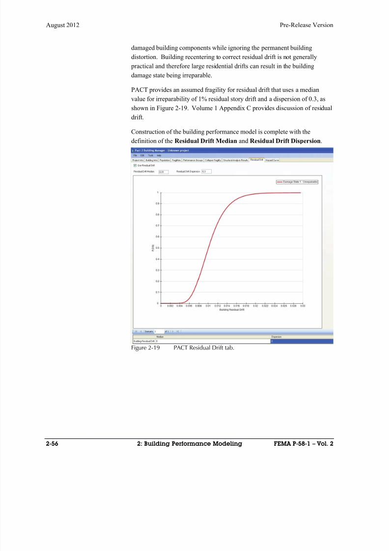
8/12/2019 Seismic Performance Assessment of Buildings
http://slidepdf.com/reader/full/seismic-performance-assessment-of-buildings 84/358
August 2012 Pre-Release Version
2-56 2: Building Performance Modeling FEMA P-58-1 – Vol. 2
damaged building components while ignoring the permanent building
distortion. Building recentering to correct residual drift is not generally
practical and therefore large residential drifts can result in the building
damage state being irreparable.
PACT provides an assumed fragility for residual drift that uses a medianvalue for irreparability of 1% residual story drift and a dispersion of 0.3, as
shown in Figure 2-19. Volume 1 Appendix C provides discussion of residual
drift.
Construction of the building performance model is complete with the
definition of the Residual Drift Median and Residual Drift Dispersion.
Figure 2-19 PACT Residual Drift tab.
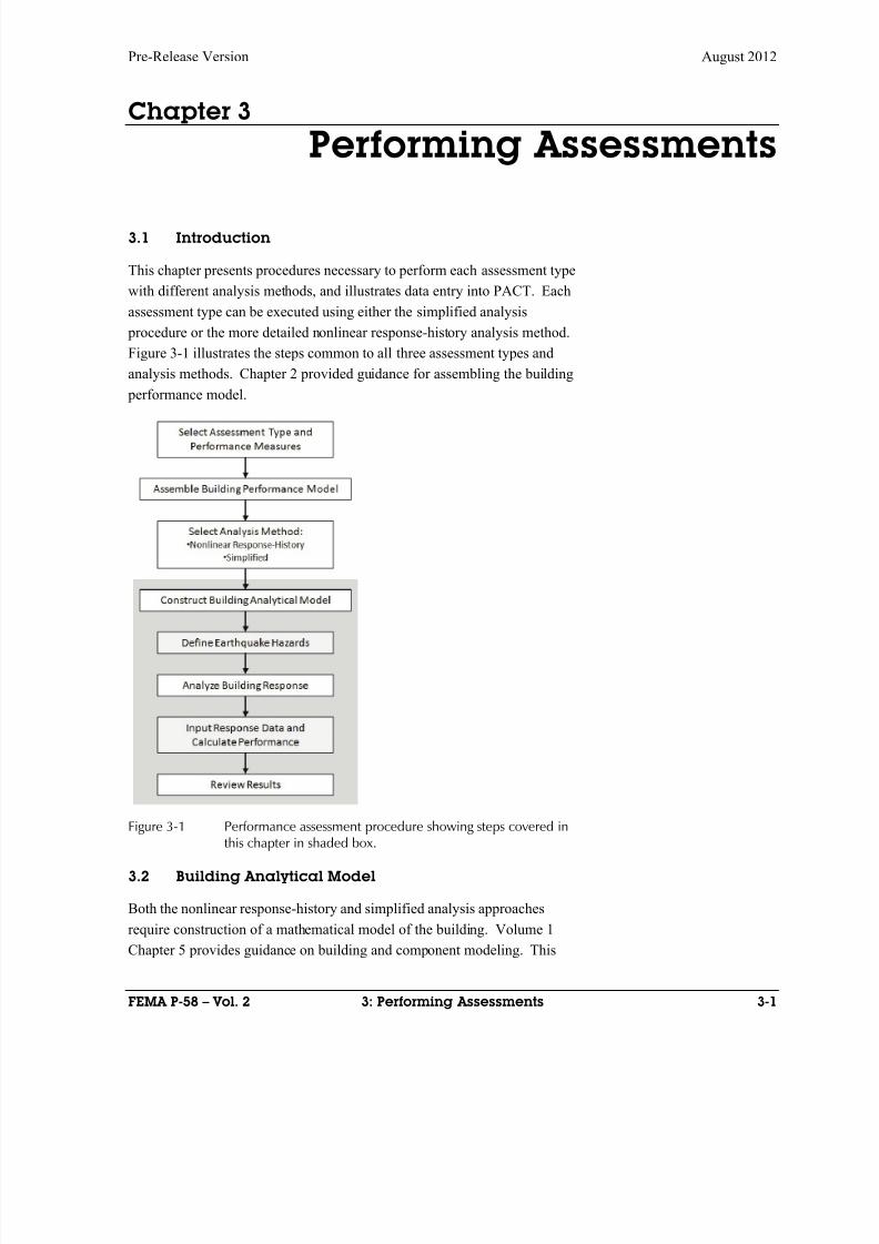
8/12/2019 Seismic Performance Assessment of Buildings
http://slidepdf.com/reader/full/seismic-performance-assessment-of-buildings 85/358
Pre-Release Version August 2012
FEMA P-58 – Vol. 2 3: Performing Assessments 3-1
Chapter 3
Performing Assessments
3.1 Introduction
This chapter presents procedures necessary to perform each assessment type
with different analysis methods, and illustrates data entry into PACT. Each
assessment type can be executed using either the simplified analysis
procedure or the more detailed nonlinear response-history analysis method.
Figure 3-1 illustrates the steps common to all three assessment types and
analysis methods. Chapter 2 provided guidance for assembling the building
performance model.
Figure 3-1 Performance assessment procedure showing steps covered inthis chapter in shaded box.
3.2 Building Analytical Model
Both the nonlinear response-history and simplified analysis approaches
require construction of a mathematical model of the building. Volume 1
Chapter 5 provides guidance on building and component modeling. This
8/12/2019 Seismic Performance Assessment of Buildings
http://slidepdf.com/reader/full/seismic-performance-assessment-of-buildings 86/358
August 2012 Pre-Release Version
3-2 3: Performing Assessments FEMA P-58 – Vol. 2
section summarizes some basic modeling considerations that support
execution of the analyses presented in later sections.
3.2.1 Nonlinear Response-History Analysis
A building should be modeled as a three-dimensional assembly of
components including foundations and soils as appropriate. Two
dimensional models are not recommended for response history analyses. If
two-dimensional models are used, an individual model is required for each of
the building’s primary response directions, with ground motion pairs applied
such that one component is used in the model for direction 1 and the second
for the model representing direction 2.
Components should be modeled over their full range of expected
deformation response using hysteretic properties based upon test data.
Where test data are lacking, idealized backbone curves, as described in
ASCE 41-06 (ASCE, 2007), can be used. The model should explicitly
include component strength and stiffness degradation. Volume 1 Chapter 5
provides a more detailed discussion of component degradation modeling.
Median values of component properties, such as yield deformation, yield
strength, and capping strength, should be used. Mean or expected values may
be substituted where insufficient information is available to accurately
capture a median value.
Models should include dead and expected live loads acting throughout the
building. Live loads can be taken as 25% of the code specified design live
load without further reduction for influence area.
Equivalent viscous damping should generally be limited to 1 to 5% of critical
damping to account for the effects of nonstructural components and soil-
structure interaction not explicitly included in the analytical model. The
majority of energy dissipated during building response should be generated
by the hysteric behavior of the modeled components.
Soil-structure interaction and foundation embedment effects can be modeled
explicitly or accounted for using approximate methods (e.g., FEMA 440).
Volume 1 Appendix B provides guidance and discussion of these topics. Theresponse of relatively stiff buildings on relatively soft soils and buildings
with a basement that extends more than one story beneath grade can be
significantly affected by soil structure interaction.
Models should be structured to return values of the demand parameters
associated with the fragility specifications used to assess performance. For
example, eccentric-braced frame fragility functions use link beam rotation as

8/12/2019 Seismic Performance Assessment of Buildings
http://slidepdf.com/reader/full/seismic-performance-assessment-of-buildings 87/358
Pre-Release Version August 2012
FEMA P-58 – Vol. 2 3: Performing Assessments 3-3
the demand parameter. Models of eccentrically braced frame structures
should be configured to provide this demand value. Values for story drift
ratio should reflect only the racking drift ratio component of total story drift
ratio and not the contribution attributable to rotation from lower floors of the
building. For taller structures and those that include wall systems, one means
of obtaining this drift ratio is to include low-stiffness, elastic, cross brace
members whose elongation will not be influenced by the rotational effects of
the components below. The elongation (or shortening of these members) can
be used to calculate shear drift ratio.
To the extent possible, the model should explicitly include the range of
component deformation to failure. Where this cannot be done, users should
estimate the deformation limits at which failure of these components is likely
to occur. Users should carefully review analysis results and adjust them to
account for these non-simulated component failures.
3.2.2 Simplified Analysis
The simplified procedure uses a linear elastic structural model and an
estimate of the building’s lateral yield strength to estimate response, and
determine estimated median values of peak story drift ratios, residual drift
ratios, peak floor acceleration and floor velocity. Building response is
assumed to be uncoupled along the principal horizontal building axes.
Separate analyses are performed for each response direction. The simplified
procedure assumes the following:
Building response along each horizontal axis is uncoupled;
The building is regular in plan and elevation (i.e. there are no substantial
discontinuities in lateral strength and stiffness);
Story drifts do not exceed four times the corresponding yield drift, so
that assumptions of elastic-plastic (bilinear) response at the component
level is not substantially compromised by excessive degradation in
strength and stiffness;
The story drift ratios are less than 4%, beyond which P-∆ effects may
become important; and
The building is less than 15 stories in height, minimizing the potential for
significant higher mode effects.
If the building being assessed does not conform to these assumptions, the
simplified procedure may produce unreliable results.
8/12/2019 Seismic Performance Assessment of Buildings
http://slidepdf.com/reader/full/seismic-performance-assessment-of-buildings 88/358
8/12/2019 Seismic Performance Assessment of Buildings
http://slidepdf.com/reader/full/seismic-performance-assessment-of-buildings 89/358
Pre-Release Version August 2012
FEMA P-58 – Vol. 2 3: Performing Assessments 3-5
geometric mean of 2 orthogonal horizontal components of ground motion.
The guidance for ground motion selection and scaling provided in Volume 1
is summarized below and presented with the following steps:
Step 1. Determine the building’s fundamental translational periods in two
orthogonal directions (T 1 X
and T 1Y
).
Step 2. Determine the effective first mode period T as the average of T 1 X
and T 1Y if response in the two directions are uncoupled and as the larger of
T 1 X or T 1
Y if response is coupled.
Step 3. Using the target response spectrum, extract the S a value.
Step 4. Select a candidate suite of recorded ground motion pairs having
geomean spectral shape similar to the target spectrum. Recorded ground
motions are available from a number of sources including:
www.peer.berkeley.edu and www.cosmos-eq.org.
Step 5. Construct the geomean response spectrum for each ground motion
pair using the equation:
gm x yS S T S T
Step 6. Determine the periods T min and T max over which the suite of ground
motion pairs are scaled to be consistent with the target spectrum. T max is
obtained from the equation:
2maxT T
Period T min should typically be taken as the smaller of 0.2T 1 X
or 0.2T 1Y
. Ifsubstantial damage can occur due to response in modes having periods
smaller than T min, e.g., in high-rise buildings where multiple higher modes
may contribute significantly to the acceleration and drift response, select T min
sufficiently small to capture these important response modes.
Step 7. Compare each pair’s geomean spectral shape with that of the target
spectrum over the range T min to T max. Select ground motion pairs with
geomean spectra that are similar in shape to the target response spectrum
within that range. Discard motion pairs that do not fit the shape of the target
spectrum adequately.
Step 8. Amplitude-scale both components of each ground motion pair by the
ratio of T S a obtained from the target spectrum to that of the geomean
spectrum for the pair.
Figure 3-2 shows scaled spectra for a suite of 5 motions selected for
intensity-based assessment of a structure with 5.0T seconds. The ground
motion pairs were selected with geomean spectral shape similar to the target
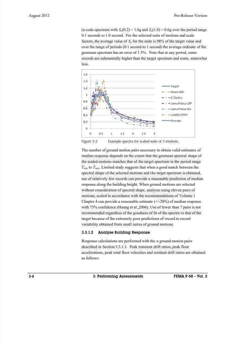
8/12/2019 Seismic Performance Assessment of Buildings
http://slidepdf.com/reader/full/seismic-performance-assessment-of-buildings 90/358
August 2012 Pre-Release Version
3-6 3: Performing Assessments FEMA P-58 – Vol. 2
(a code-spectrum with S a(0.2) = 1.0g and S a(1.0) = 0.6g over the period range
0.1 seconds to 1.0 second. For the selected suite of motions and scale
factors, the average value of S a for the suite is 98% of the target value and
over the range of periods (0.1 second to 1 second) the average ordinate of the
geomean spectrum has an error of 1.5%. Note that at any period, some
records are substantially higher than the target spectrum and some, somewhat
less.
Figure 3-2 Example spectra for scaled suite of 5 motions.
The number of ground motion pairs necessary to obtain valid estimates of
median response depends on the extent that the geomean spectral shape of
the scaled motions matches that of the target spectrum in the period range
T min to T max. Limited study suggests that when a good match between thespectral shape of the selected motions and the target spectrum is obtained,
use of relatively few records can provide a reasonable prediction of median
response along the building height. When ground motions are selected
without consideration of spectral shape, analyses using eleven pairs of
motions, scaled in accordance with the recommendations of Volume 1
Chapter 4 can provide a reasonable estimate (+/-20%) of median response
with 75% confidence (Huang et al.,2006). Use of fewer than 7 pairs is not
recommended regardless of the goodness of fit of the spectra to that of the
target because of the extremely poor predictions of record to record
variability obtained from small suites of ground motions.
3.3.1.2 Analyze Building Response
Response calculations are performed with the n ground motion pairs
described in Section 3.3.1.1. Peak transient drift ratios, peak floor
accelerations, peak total floor velocities and residual drift ratios are obtained
as follows:
8/12/2019 Seismic Performance Assessment of Buildings
http://slidepdf.com/reader/full/seismic-performance-assessment-of-buildings 91/358
8/12/2019 Seismic Performance Assessment of Buildings
http://slidepdf.com/reader/full/seismic-performance-assessment-of-buildings 92/358
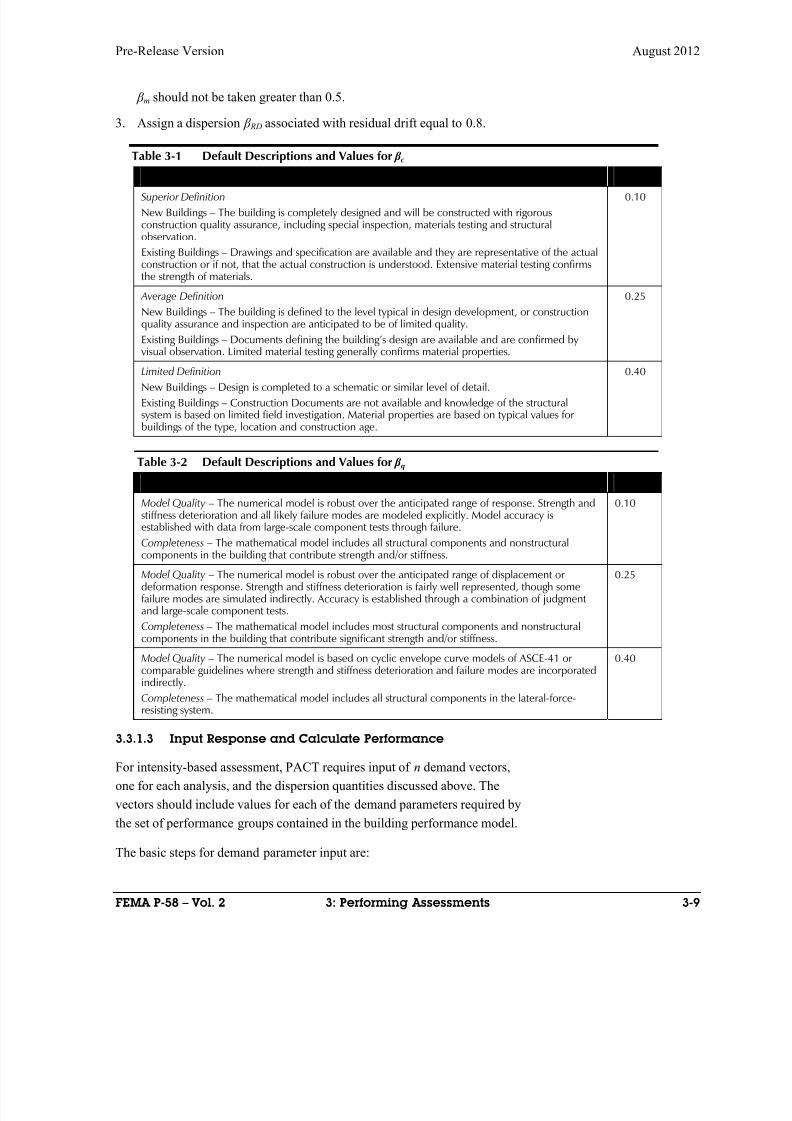
8/12/2019 Seismic Performance Assessment of Buildings
http://slidepdf.com/reader/full/seismic-performance-assessment-of-buildings 93/358
Pre-Release Version August 2012
FEMA P-58 – Vol. 2 3: Performing Assessments 3-9
β m should not be taken greater than 0.5.
3. Assign a dispersion β RD associated with residual drift equal to 0.8.
Table 3-1 Default Descriptions and Values for β c
Definition and Construction Quality Assurance β c
Superior Definition
New Buildings – The building is completely designed and will be constructed with rigorousconstruction quality assurance, including special inspection, materials testing and structuralobservation.
Existing Buildings – Drawings and specification are available and they are representative of the actualconstruction or if not, that the actual construction is understood. Extensive material testing confirmsthe strength of materials.
0.10
Average Definition
New Buildings – The building is defined to the level typical in design development, or constructionquality assurance and inspection are anticipated to be of limited quality.
Existing Buildings – Documents defining the building’s design are available and are confirmed byvisual observation. Limited material testing generally confirms material properties.
0.25
Limited Definition
New Buildings – Design is completed to a schematic or similar level of detail.
Existing Buildings – Construction Documents are not available and knowledge of the structuralsystem is based on limited field investigation. Material properties are based on typical values forbuildings of the type, location and construction age.
0.40
Table 3-2 Default Descriptions and Values for β q
Model Quality and Completeness β q
Model Quality – The numerical model is robust over the anticipated range of response. Strength andstiffness deterioration and all likely failure modes are modeled explicitly. Model accuracy isestablished with data from large-scale component tests through failure.
Completeness – The mathematical model includes all structural components and nonstructuralcomponents in the building that contribute strength and/or stiffness.
0.10
Model Quality – The numerical model is robust over the anticipated range of displacement ordeformation response. Strength and stiffness deterioration is fairly well represented, though somefailure modes are simulated indirectly. Accuracy is established through a combination of judgmentand large-scale component tests.
Completeness – The mathematical model includes most structural components and nonstructuralcomponents in the building that contribute significant strength and/or stiffness.
0.25
Model Quality – The numerical model is based on cyclic envelope curve models of ASCE-41 orcomparable guidelines where strength and stiffness deterioration and failure modes are incorporatedindirectly.
Completeness – The mathematical model includes all structural components in the lateral-force-resisting system.
0.40
3.3.1.3 Input Response and Calculate Performance
For intensity-based assessment, PACT requires input of n demand vectors,
one for each analysis, and the dispersion quantities discussed above. The
vectors should include values for each of the demand parameters required by
the set of performance groups contained in the building performance model.
The basic steps for demand parameter input are:
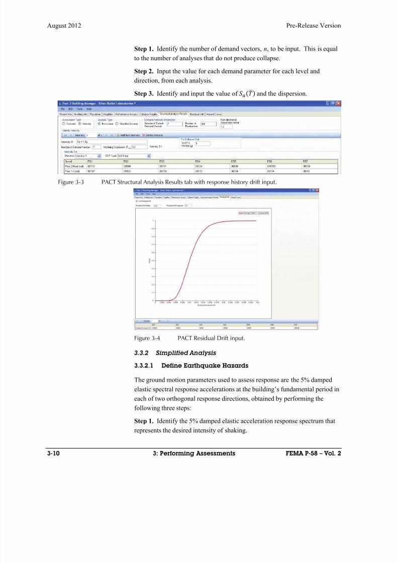
8/12/2019 Seismic Performance Assessment of Buildings
http://slidepdf.com/reader/full/seismic-performance-assessment-of-buildings 94/358
August 2012 Pre-Release Version
3-10 3: Performing Assessments FEMA P-58 – Vol. 2
Step 1. Identify the number of demand vectors, n, to be input. This is equal
to the number of analyses that do not produce collapse.
Step 2. Input the value for each demand parameter for each level and
direction, from each analysis.
Step 3. Identify and input the value of and the dispersion.
Figure 3-3 PACT Structural Analysis Results tab with response history drift input.
Figure 3-4 PACT Residual Drift input.
3.3.2 Simplified Analysis
3.3.2.1 Define Earthquake Hazards
The ground motion parameters used to assess response are the 5% damped
elastic spectral response accelerations at the building’s fundamental period in
each of two orthogonal response directions, obtained by performing the
following three steps:
Step 1. Identify the 5% damped elastic acceleration response spectrum that
represents the desired intensity of shaking.
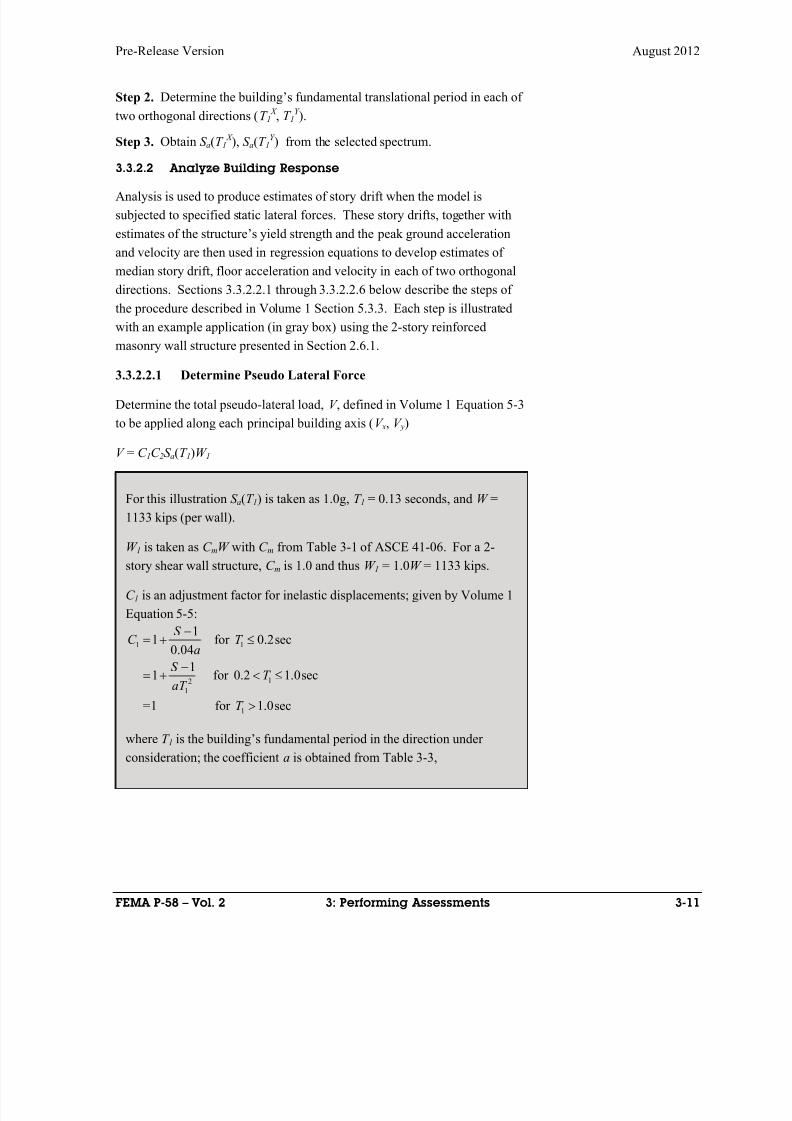
8/12/2019 Seismic Performance Assessment of Buildings
http://slidepdf.com/reader/full/seismic-performance-assessment-of-buildings 95/358
Pre-Release Version August 2012
FEMA P-58 – Vol. 2 3: Performing Assessments 3-11
Step 2. Determine the building’s fundamental translational period in each of
two orthogonal directions (T 1 X , T 1
Y ).
Step 3. Obtain S a(T 1 X ), S a(T 1
Y ) from the selected spectrum.
3.3.2.2 Analyze Building Response
Analysis is used to produce estimates of story drift when the model is
subjected to specified static lateral forces. These story drifts, together with
estimates of the structure’s yield strength and the peak ground acceleration
and velocity are then used in regression equations to develop estimates of
median story drift, floor acceleration and velocity in each of two orthogonal
directions. Sections 3.3.2.2.1 through 3.3.2.2.6 below describe the steps of
the procedure described in Volume 1 Section 5.3.3. Each step is illustrated
with an example application (in gray box) using the 2-story reinforced
masonry wall structure presented in Section 2.6.1.
3.3.2.2.1 Determine Pseudo Lateral Force
Determine the total pseudo-lateral load, V , defined in Volume 1 Equation 5-3
to be applied along each principal building axis (V x, V y)
V = C 1C 2S a(T 1)W 1
For this illustration S a(T 1) is taken as 1.0g, T 1 = 0.13 seconds, and W =
1133 kips (per wall).
W 1 is taken as C mW with C m from Table 3-1 of ASCE 41-06. For a 2-story shear wall structure, C m is 1.0 and thus W 1 = 1.0W = 1133 kips.
C 1 is an adjustment factor for inelastic displacements; given by Volume 1
Equation 5-5:
where T 1 is the building’s fundamental period in the direction under
consideration; the coefficient a is obtained from Table 3-3,
1 1
12
1
1
11 for 0.2sec
0.04
11 for 0.2 1.0sec
=1 for 1.0sec
S C T
a
S T
aT
T

8/12/2019 Seismic Performance Assessment of Buildings
http://slidepdf.com/reader/full/seismic-performance-assessment-of-buildings 96/358
August 2012 Pre-Release Version
3-12 3: Performing Assessments FEMA P-58 – Vol. 2
Table 3-3 Values of coefficient a
ASCE 7-10 Site Class a
A 130
B 130
C 90
D 60
E 60
and where S is a strength ratio given by Volume 1 Equation 5-6:
1
1
a
y
S T W S
V
In this equation, V y1 is the story yield strength in the direction under
consideration. V y1 can be calculated using the following three differentapproaches.
Plastic Analysis Method
For a shear wall system the equivalent lateral force distribution produces a
base moment on the wall. The ratio of this moment to the base shear is
designated the spear span, H 0. Up until yielding at the wall’s base occurs,
the vertical force distribution procedure defined in the next step (Section
3.3.2.2.2) can be used to determine the shear span. The shear span can be
used to define the relationship between base shear at yield and wall
moment at yield.
Structural systems that include concentrically braced steel frames; squat
walls or moment frames generally will not require an estimation of the
vertical distribution of forces on the building. The calculation of story
yield for these systems is predominantly dictated by the story shear only.
For taller structures, the effects of overturning may reduce the story yield
force and thus should be considered for all structural systems.
As defined in Section 3.3.2.2.2, the story force distribution of a 1 kip base
shear is 0.63 kips at the roof and 0.37 kips at the second floor. For a 1 kip
base shear, the flexural demand at the base of the walls will be:
M 0 = 0.63(20) + 0.37(10) = 16.3 kip-ft;
the shear span is defined as 16.3/1 = 16.3 feet
The calculated yield capacity using the nominal yield properties of one of
the masonry walls in the building is equal to 5189k-1. The shear force
required to produce this moment is
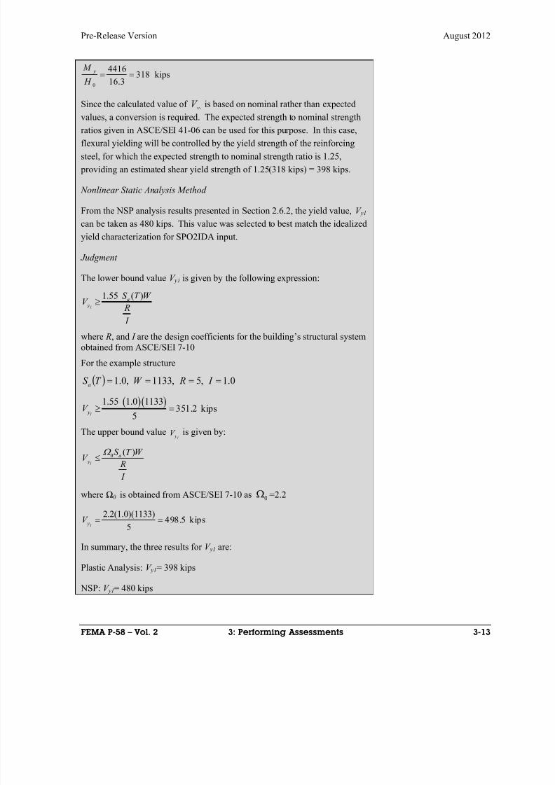
8/12/2019 Seismic Performance Assessment of Buildings
http://slidepdf.com/reader/full/seismic-performance-assessment-of-buildings 97/358
Pre-Release Version August 2012
FEMA P-58 – Vol. 2 3: Performing Assessments 3-13
0
4416318 kips
16.3
y M
H
Since the calculated value of1 yV is based on nominal rather than expected
values, a conversion is required. The expected strength to nominal strength
ratios given in ASCE/SEI 41-06 can be used for this purpose. In this case,
flexural yielding will be controlled by the yield strength of the reinforcing
steel, for which the expected strength to nominal strength ratio is 1.25,
providing an estimated shear yield strength of 1.25(318 kips) = 398 kips.
Nonlinear Static Analysis Method
From the NSP analysis results presented in Section 2.6.2, the yield value, V y1
can be taken as 480 kips. This value was selected to best match the idealized
yield characterization for SPO2IDA input.
Judgment
The lower bound value V y1 is given by the following expression:
1.55 ( )1
a y
S T W V
R
I
where R, and I are the design coefficients for the building’s structural systemobtained from ASCE/SEI 7-10
For the example structure
0.1,5,1133,0.1 I RW T S
a
1.55 1.0 1133351.2 kips
51 yV
The upper bound value1 yV is given by:
0 ( )1
a y
S T W V
R
I
where Ω0 is obtained from ASCE/SEI 7-10 as 0 =2.2
2.2(1.0)(1133) 498.5 kips51 yV
In summary, the three results for V y1 are:
Plastic Analysis: V y1= 398 kips
NSP: V y1= 480 kips

8/12/2019 Seismic Performance Assessment of Buildings
http://slidepdf.com/reader/full/seismic-performance-assessment-of-buildings 98/358
August 2012 Pre-Release Version
3-14 3: Performing Assessments FEMA P-58 – Vol. 2
Judgment: 351.2 kips ≤ V y1 ≤ 498.5 kips
For illustration in the continuation of this example, V y1 will be taken as 398
kips, based on the plastic analysis method above.
Returning to the calculation of S,
(1.0)(1133)
2.85398S
Since T 1 < 0.2s
a
S C
04.0
111
The structure is located on Site Class D soil, therefore from Table 3-3, 60a
and 77.1)60(04.0
185.211
C
For S greater than 1.0, C 2 (an adjustment factor for cyclic degradation) is
given by Volume 1 Equation 5-7 as follows:
2
2 1
2
12
1
1
11 for 0.2 seconds
32
11=1+ for 0.2 0.7 seconds
800
=1 for 0.7 seconds
S C T
S T
T
T
Since sT 2.01
11.1
32
85.11
32
11
22
2
S
C
thus V = (1.77)(1.11)(1.0)(1133)
V = 2226 kips
3.3.2.2.2 Estimate Median Story Drift and Dispersion
Estimate of median story drift is calculated following the five steps below.
Dispersion is estimated by using the default values of the dispersion given in
Volume 1 Chapter 5.
Step 1. Determine the vertical distribution of force over the height of the
building according to Volume 1 Equation 5-8 where F x is the lateral load at
each floor level x:
F x = C vxV
where C vx according to Volume 1 Equation 5-9 is:
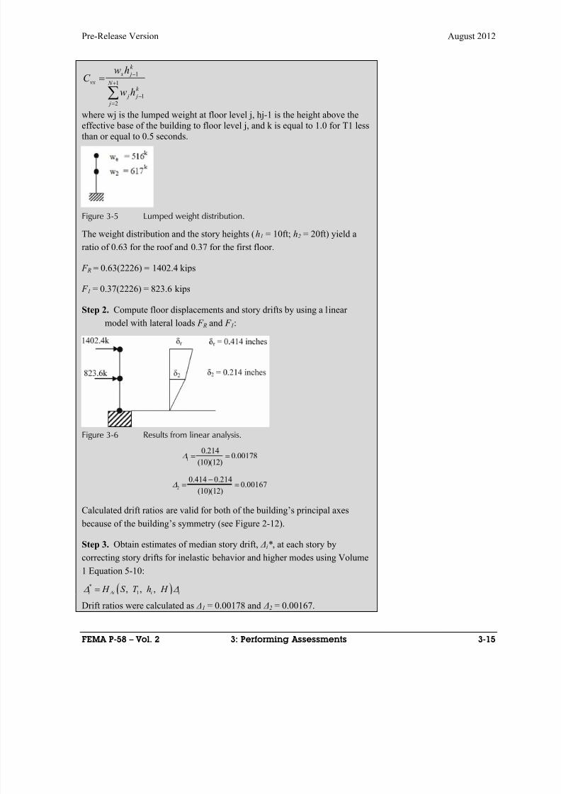
8/12/2019 Seismic Performance Assessment of Buildings
http://slidepdf.com/reader/full/seismic-performance-assessment-of-buildings 99/358
Pre-Release Version August 2012
FEMA P-58 – Vol. 2 3: Performing Assessments 3-15
k
j
N
j
j
k
j x
vx
hw
hwC
1
1
2
1
where wj is the lumped weight at floor level j, hj-1 is the height above the
effective base of the building to floor level j, and k is equal to 1.0 for T1 lessthan or equal to 0.5 seconds.
Figure 3-5 Lumped weight distribution.
The weight distribution and the story heights (h1 = 10ft; h2 = 20ft) yield a
ratio of 0.63 for the roof and 0.37 for the first floor.
F R = 0.63(2226) = 1402.4 kips
F 1 = 0.37(2226) = 823.6 kips
Step 2. Compute floor displacements and story drifts by using a linear
model with lateral loads F R and F 1:
Figure 3-6 Results from linear analysis.
1
0.2140.00178
(10)(12)
2
0.414 0.2140.00167
(10)(12)
Calculated drift ratios are valid for both of the building’s principal axes
because of the building’s symmetry (see Figure 2-12).
Step 3. Obtain estimates of median story drift, Δi*, at each story by
correcting story drifts for inelastic behavior and higher modes using Volume
1 Equation 5-10:
*
1, , ,i i i i H S T h H
Drift ratios were calculated as Δ1 = 0.00178 and Δ2 = 0.00167.
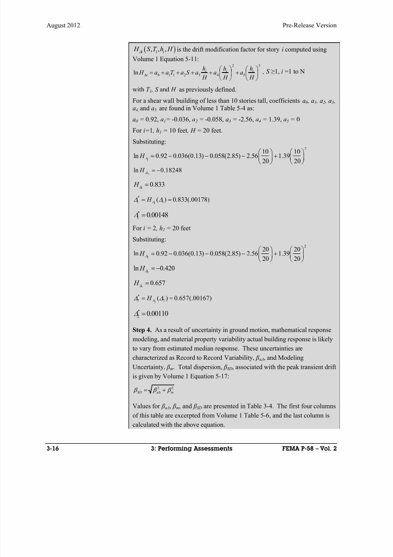
8/12/2019 Seismic Performance Assessment of Buildings
http://slidepdf.com/reader/full/seismic-performance-assessment-of-buildings 100/358
August 2012 Pre-Release Version
3-16 3: Performing Assessments FEMA P-58 – Vol. 2
1, , ,i i H S T h H is the drift modification factor for story i computed using
Volume 1 Equation 5-11:3
5
2
432110ln
H
ha
H
ha
H
haS aT aa H iii
i , S ≥1, i =1 to N
with T 1 , S and H as previously defined.For a shear wall building of less than 10 stories tall, coefficients a0 , a1 , a2 , a3 ,a4, and a5 are found in Volume 1 Table 5-4 as:
a0 = 0.92, a1= -0.036, a2 = -0.058, a3 = -2.56, a4 = 1.39, a5 = 0
For i=1 , h1 = 10 feet , H = 20 feet.
Substituting:
1
210 10
ln 0.92 0.036(0.13) 0.058(2.85) 2.56 1.3920 20
H
1ln 0.18248 H
10.833 H
1
*
1 1( ) 0.833(.00178) H
*
1 0.00148
For i = 2 , h2 = 20 feet
Substituting:
2
220 20
ln 0.92 0.036(0.13) 0.058(2.85) 2.56 1.3920 20
H
2ln 0.420 H
20.657 H
2
*
2 2( ) 0.657(.00167) H
*
2 0.00110
Step 4. As a result of uncertainty in ground motion, mathematical response
modeling, and material property variability actual building response is likely
to vary from estimated median response. These uncertainties are
characterized as Record to Record Variability, β a Δ, and Modeling
Uncertainty, β m. Total dispersion, β SD, associated with the peak transient drift
is given by Volume 1 Equation 5-17:
22
maSD
Values for β a Δ, β m, and β SD are presented in Table 3-4. The first four columns
of this table are excerpted from Volume 1 Table 5-6, and the last column is
calculated with the above equation.
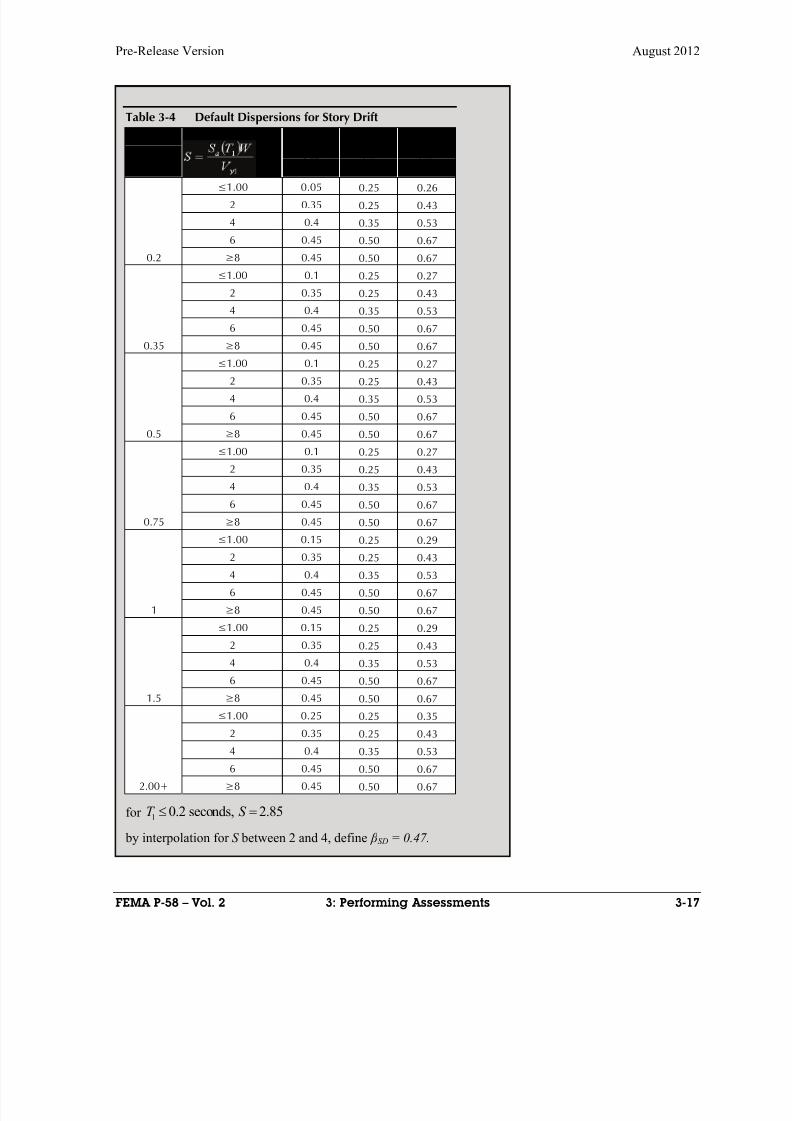
8/12/2019 Seismic Performance Assessment of Buildings
http://slidepdf.com/reader/full/seismic-performance-assessment-of-buildings 101/358
8/12/2019 Seismic Performance Assessment of Buildings
http://slidepdf.com/reader/full/seismic-performance-assessment-of-buildings 102/358
August 2012 Pre-Release Version
3-18 3: Performing Assessments FEMA P-58 – Vol. 2
3.3.2.2.3 Estimate Median Peak Floor Acceleration and Dispersion
Peak acceleration at the building base is taken as peak ground acceleration.
At other floor levels, estimate the median peak floor acceleration by
following the two steps below. Dispersion is estimated by using the default
values of the dispersion given in Volume 1 Chapter 5.
Step 1. Obtain estimates of median peak floor acceleration, ai*, at each story
above the building base by correcting peak ground accelerations using
Volume 1 Equation 5-12:
pga H hT S H a iaii ,,, 1
*
1,12 S N toi
For this example, pga = 0.40g.
H ai is the acceleration correction factor for floor i given by Volume 1
Equation 5-13:
2 3
0 1 1 2 3 4 5ln , 1, 2 1i i iai
h h h H a a T a S a a a S i to N
H H H
with T 1, S, and H as previously defined.
For a shear wall building of less than 10 stories tall, coefficients a0 , a1 , a2 , a3 ,
a4 and a5 are found in Volume 1 Table 5-4 as:
a0 = 0.66, a1 = -0.15, a2 = -0.084, a3 = -0.26, a4 = 0.57, a5 = 0
For Floor 1 (at grade)
pgaa *
1 *
1 0.40a g
For Floor 2 ,
5.020
101 H
h
2
2 5.57.0)5.0(26.0)85.2(084.0)13(.15.066.0ln a H
4136.0ln 2 a H
and 512.12 a H
g a 605.0)4.0(512.1*
2
For Floor 3 (roof),
0.120
202 H
h
2
3 157.0)0.1(26.0)85.2(084.0)13(.15.066.0ln a H
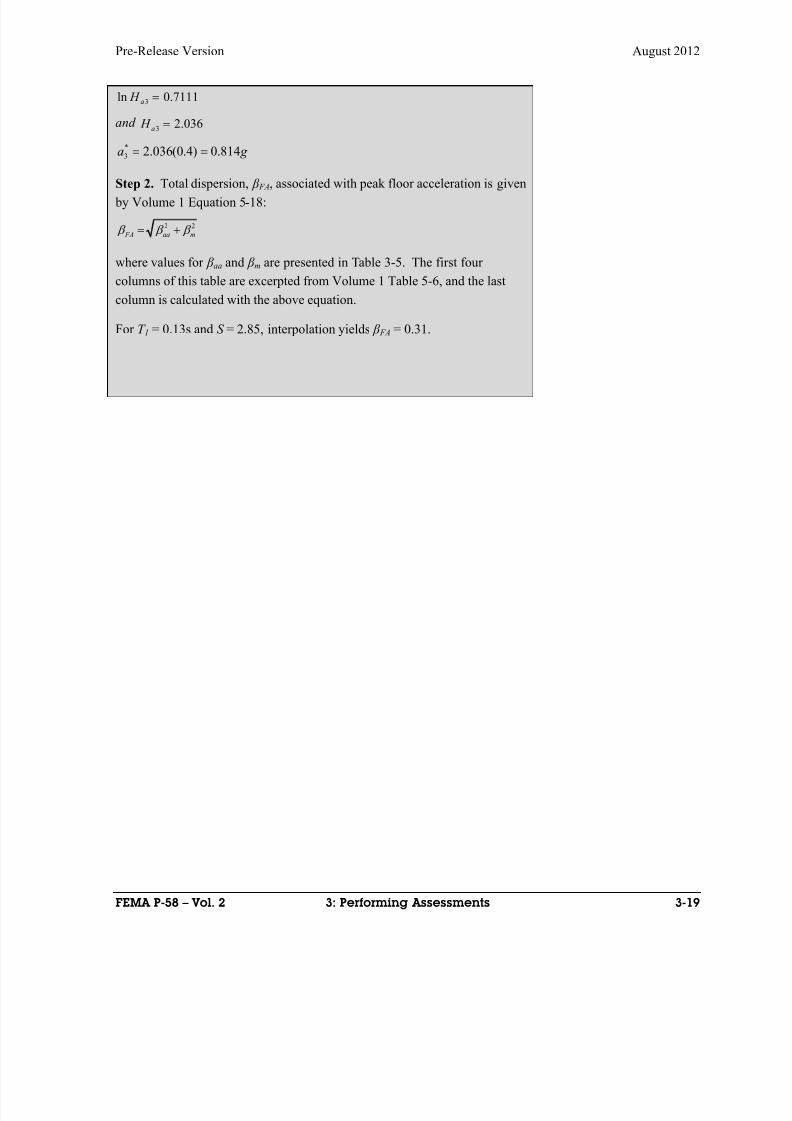
8/12/2019 Seismic Performance Assessment of Buildings
http://slidepdf.com/reader/full/seismic-performance-assessment-of-buildings 103/358
Pre-Release Version August 2012
FEMA P-58 – Vol. 2 3: Performing Assessments 3-19
7111.0ln 3 a H
and 036.23 a H
g a 814.0)4.0(036.2*
3
Step 2. Total dispersion, β FA, associated with peak floor acceleration is given by Volume 1 Equation 5-18:
22
maa FA
where values for β aa and β m are presented in Table 3-5. The first four
columns of this table are excerpted from Volume 1 Table 5-6, and the last
column is calculated with the above equation.
For T 1 = 0.13s and S = 2.85, interpolation yields β FA = 0.31.
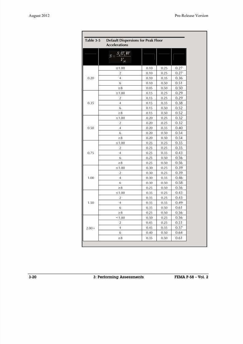
8/12/2019 Seismic Performance Assessment of Buildings
http://slidepdf.com/reader/full/seismic-performance-assessment-of-buildings 104/358
August 2012 Pre-Release Version
3-20 3: Performing Assessments FEMA P-58 – Vol. 2
Table 3-5 Default Dispersions for Peak Floor Accelerations
T 1 (sec) β aa β m β FA
0.20
≤1.00 0.10 0.25 0.27
2 0.10 0.25 0.27
4 0.10 0.35 0.36
6 0.10 0.50 0.51
≥8 0.05 0.50 0.50
0.35
≤1.00 0.15 0.25 0.29
2 0.15 0.25 0.29
4 0.15 0.35 0.38
6 0.15 0.50 0.52
≥8 0.15 0.50 0.52
0.50
≤1.00 0.20 0.25 0.32
2 0.20 0.25 0.32
4 0.20 0.35 0.40
6 0.20 0.50 0.54
≥8 0.20 0.50 0.54
0.75
≤1.00 0.25 0.25 0.35
2 0.25 0.25 0.35
4 0.25 0.35 0.43
6 0.25 0.50 0.56
≥8 0.25 0.50 0.56
1.00
≤
1.00 0.30 0.25 0.39 2 0.30 0.25 0.39
4 0.30 0.35 0.46
6 0.30 0.50 0.58
≥8 0.25 0.50 0.56
1.50
≤1.00 0.35 0.25 0.43
2 0.35 0.25 0.43
4 0.35 0.35 0.49
6 0.35 0.50 0.61
≥8 0.25 0.50 0.56
2.00+
≤1.00 0.50 0.25 0.56
2 0.45 0.25 0.51
4 0.45 0.35 0.57
6 0.40 0.50 0.64
≥8 0.35 0.50 0.61

8/12/2019 Seismic Performance Assessment of Buildings
http://slidepdf.com/reader/full/seismic-performance-assessment-of-buildings 105/358
Pre-Release Version August 2012
FEMA P-58 – Vol. 2 3: Performing Assessments 3-21
3.3.2.2.4 Estimate Median Peak Total Floor Velocity and Dispersion
Estimate the median peak total floor velocity by following the two steps
below. Dispersion is estimated by using the default values of the dispersion
given in Volume 1 Chapter 5.
Step 1. A reference floor velocity at level i is obtained from Volume 1
Equation 5-16:
3.0/2
1
1
11
r
i y
si g W
V T PGV v
where:
T 1 = 0.13 seconds
1 yV = 398 kips
g
W 1 = 1.0W = g
1133 kips
Γ 1 =W
W 1 = 1.0,
δr = 00173.0)12)(20(
414.0
Determine PGV
2 21 0.4g 0.4 386 in / sec 154in / secaS from site hazard data.
2154in / sec1 1
1 24.5in / sec2 2
a
v
S
S
1 24.5in / sec14.5in / sec
1.65 1.65
vS PGV
For Floor 1: For the first floor or grade level, peak total floor velocity equals
the peak ground velocity.
1 PGV 14.5in / sec sv
For Floor 2:
Δ1 = .00178
2
.13 398 0.0017814.5in / sec 0.3 1.0
2 1133 / 386 0.00173 sv
2 15.3 in / sec sv
For Floor 3:
Δ2 = .00167

8/12/2019 Seismic Performance Assessment of Buildings
http://slidepdf.com/reader/full/seismic-performance-assessment-of-buildings 106/358
August 2012 Pre-Release Version
3-22 3: Performing Assessments FEMA P-58 – Vol. 2
2
.13 398 0.0016714.5in / sec 0.3 1.0
2 1133 / 386 0.00173 sv
2 15.3 in / sec sv
Step 2. Convert calculated Peak Total Floor Velocity to median estimate of
Peak Total Floor Velocity
Median values of Peak Total Floor Velocity are as:
siivi si v H hT S H v ,,, 1*
where H vi is the velocity modification factor for floor I, given by Volume 1
Equation 5-15:
2 3
0 1 1 2 3 4 5ln , 1 , 2 1i i ivi
h h h H a a T a S a a a S i to N
H H h
with T 1 and H as previously defined and S >1.
For a shear wall building of less than 10 stories tall, coefficients a0 , a1 , a2 , a3 ,
a4 and a5 are found in Volume 1 Table 5-4 as:
a0 = -0.033, a1 = -0.085, a2 = 0.055, a3 = -0.52, a4 = 0.47, a5 = 0
For Floor 1 , hi = 0, v1* = PGV = 14.5 in/sec
For Floor 2 , h1 = 10 feet
2
210 10
ln( ) 0.033 0.085(.13) 0.055(2.85) 0.52 0.4720 20
v H
0298.0)ln(2
v H , 971.02
v H
∗ 0.97115.3 / 14.9/
For Floor 3, h2 = 20 feet
0627.0)ln(3
v H , 065.13
v H
∗ 1.06515.3 / 16.3/
Step 3. Total dispersion, β FV , associated with peak total floor velocity is
given by Volume 1 Equation 5-19:
22
mav FV
Values for β av, β m, and β FV are presented in Table 3-6. The first four columns
of this table are excerpted from Volume 1 Table 5-6, and the last column is
calculated with the above equation. For
T 1 ≤ 0.2s and S = 2.85
β FV = 0.55
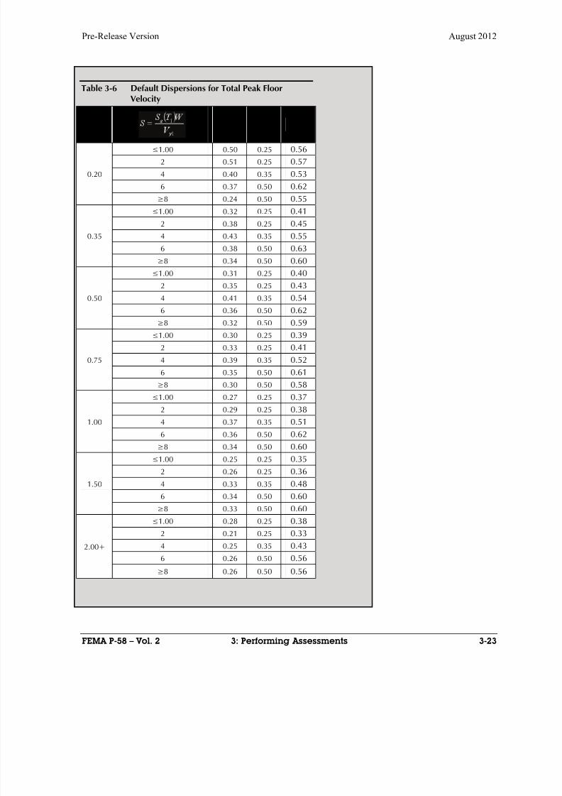
8/12/2019 Seismic Performance Assessment of Buildings
http://slidepdf.com/reader/full/seismic-performance-assessment-of-buildings 107/358
Pre-Release Version August 2012
FEMA P-58 – Vol. 2 3: Performing Assessments 3-23
Table 3-6 Default Dispersions for Total Peak Floor Velocity
T 1
(sec)
β av
β m
β FV
0.20
≤1.00 0.50 0.25 0.56
2 0.51 0.25 0.57
4 0.40 0.35 0.53
6 0.37 0.50 0.62
≥8 0.24 0.50 0.55
0.35
≤1.00 0.32 0.25 0.41
2 0.38 0.25 0.45
4 0.43 0.35 0.55
6 0.38 0.50 0.63
≥8 0.34 0.50 0.60
0.50
≤1.00 0.31 0.25 0.40
2 0.35 0.25 0.43
4 0.41 0.35 0.54
6 0.36 0.50 0.62
≥8 0.32 0.50 0.59
0.75
≤1.00 0.30 0.25 0.39
2 0.33 0.25 0.41
4 0.39 0.35 0.52
6 0.35 0.50 0.61
≥8 0.30 0.50 0.58
1.00
≤1.00 0.27 0.25 0.37
2 0.29 0.25 0.38
4 0.37 0.35 0.51
6 0.36 0.50 0.62
≥8 0.34 0.50 0.60
1.50
≤1.00 0.25 0.25 0.35
2 0.26 0.25 0.36
4 0.33 0.35 0.48
6 0.34 0.50 0.60
≥8 0.33 0.50 0.60
2.00+
≤1.00 0.28 0.25 0.38 2 0.21 0.25 0.33
4 0.25 0.35 0.43
6 0.26 0.50 0.56
≥8 0.26 0.50 0.56
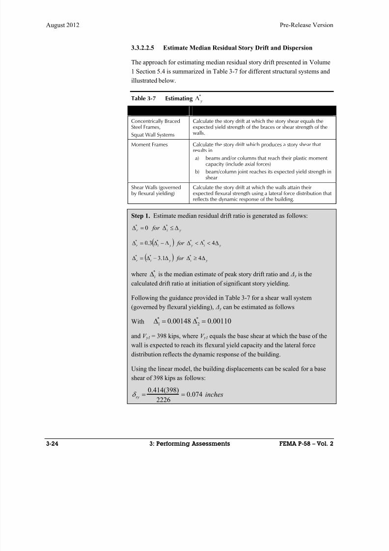
8/12/2019 Seismic Performance Assessment of Buildings
http://slidepdf.com/reader/full/seismic-performance-assessment-of-buildings 108/358
August 2012 Pre-Release Version
3-24 3: Performing Assessments FEMA P-58 – Vol. 2
3.3.2.2.5 Estimate Median Residual Story Drift and Dispersion
The approach for estimating median residual story drift presented in Volume
1 Section 5.4 is summarized in Table 3-7 for different structural systems and
illustrated below.
Table 3-7 Estimating*
y
Structural System Procedure
Concentrically BracedSteel Frames,
Squat Wall Systems
Calculate the story drift at which the story shear equals theexpected yield strength of the braces or shear strength of thewalls.
Moment Frames Calculate the story drift which produces a story shear thatresults in
a) beams and/or columns that reach their plastic momentcapacity (include axial forces)
b) beam/column joint reaches its expected yield strength in
shearShear Walls (governedby flexural yielding)
Calculate the story drift at which the walls attain theirexpected flexural strength using a lateral force distribution thatreflects the dynamic response of the building.
Step 1. Estimate median residual drift ratio is generated as follows:
yir for ** 0
yi y yir for 43.0 ****
yi yir for 41.3 ***
where *i is the median estimate of peak story drift ratio and Δ y is the
calculated drift ratio at initiation of significant story yielding.
Following the guidance provided in Table 3-7 for a shear wall system
(governed by flexural yielding), Δ y can be estimated as follows
With 00148.0*
1 00110.0*
2
and V y1 = 398 kips, where V y1 equals the base shear at which the base of the
wall is expected to reach its flexural yield capacity and the lateral force
distribution reflects the dynamic response of the building.
Using the linear model, the building displacements can be scaled for a base
shear of 398 kips as follows:
inchesry 074.02226
)398(414.0

8/12/2019 Seismic Performance Assessment of Buildings
http://slidepdf.com/reader/full/seismic-performance-assessment-of-buildings 109/358
Pre-Release Version August 2012
FEMA P-58 – Vol. 2 3: Performing Assessments 3-25
inches y 038.02226
)398(214.01
00032.0)12(10
038.01 y
63.400032.0
00148.0*1
y
Note that the Simplified Analysis method illustrated in this example was
developed for application to structures with peak transient drift demands less
than or equal to 4 times the yield drift. As drift demands exceed this level,
the simplified analysis may become less valid. Users that find that their
buildings are experiencing such large inelastic demand should consider using
the nonlinear analysis method to obtain more valid results.
The simplified method, however, predicts residual drift ratios as follows:*
1 0.00148 3.1(0.00032) 0.000488r
and*
2 0.00110 3.1(0.00032) 0.000108r
Step 2. The total dispersion associated with median values of Residual Drift
Ratio should be taken as β RD = 0.8. This includes both β a and β m.
3.3.2.3 Input Response and Calculate Performance
Simplified building response analyses produce estimated median values of
peak story drift ratios, floor accelerations, floor velocities and residual drift
ratios in each principal building response direction. PACT uses this
information to make damage state assessments for all building components
contained in the assessment model. Structural analysis results are organized
and input into PACT using the Structural Analysis Results tab (see Figure
3-7).
Figure 3-7 PACT Structural Analysis Results tab.

8/12/2019 Seismic Performance Assessment of Buildings
http://slidepdf.com/reader/full/seismic-performance-assessment-of-buildings 110/358
August 2012 Pre-Release Version
3-26 3: Performing Assessments FEMA P-58 – Vol. 2
Radio buttons and fields on the upper portion of the tab should be modified
by the user to reflect:
Assessment Type: Intensity
Analysis Type: Simplified
Number of Default Demand Vectors: This number indicates to PACT
the total number of demand vectors that may be input for each intensity
for which an assessment will be performed. The actual number of
vectors input in the lower portion of the screen can be less. Each
intensity included in the assessment can have a different number of
Demand Vectors.
Number of Realizations: PACT uses a Monte Carlo process to
determine the probability of incurring consequences. If an insufficientlylarge number of realizations are performed for each demand vector, the
indicated probability distribution may be quite inaccurate and can change
significantly each time PACT is run with the same data. The PACT
default setting is 200 realizations. This number of realizations has
generally produced stable results for repair cost and repair time. At least
500 realizations should be used for casualties and unsafe placards. Use of
larger numbers of realizations will increase PACT execution time
slightly, however, both storage time and space can increase significantly.
Non-Directional Conversion Factor: This factor sets the estimated
non-directional value of demand (story drift ratio, acceleration) as a
multiple of the maximum value of either of the directions. It is set at a
default value of 1.2, which is believed appropriate for most structures.
Under the Identify Intensity section, the user will need to depress the + Add
New Intensity button to prompt the setup for inputting intensity analysis
results. The user can then input the Intensity ID (name to identify the
intensity in the output files) and the number of demand vectors. The number
of demand vectors includes the results to be input for drift, floor acceleration
and floor velocity in each building direction. The user can also input other
demand parameters assignable to direction 1, direction 2 or nondirectional.For the simplified analysis approach, there will only be one demand vector
containing drifts, floor accelerations and floor velocities for each building
direction and each floor or story. Results should be input for all demand
types and directions that are used by the fragility specifications selected to
define damageable building components.
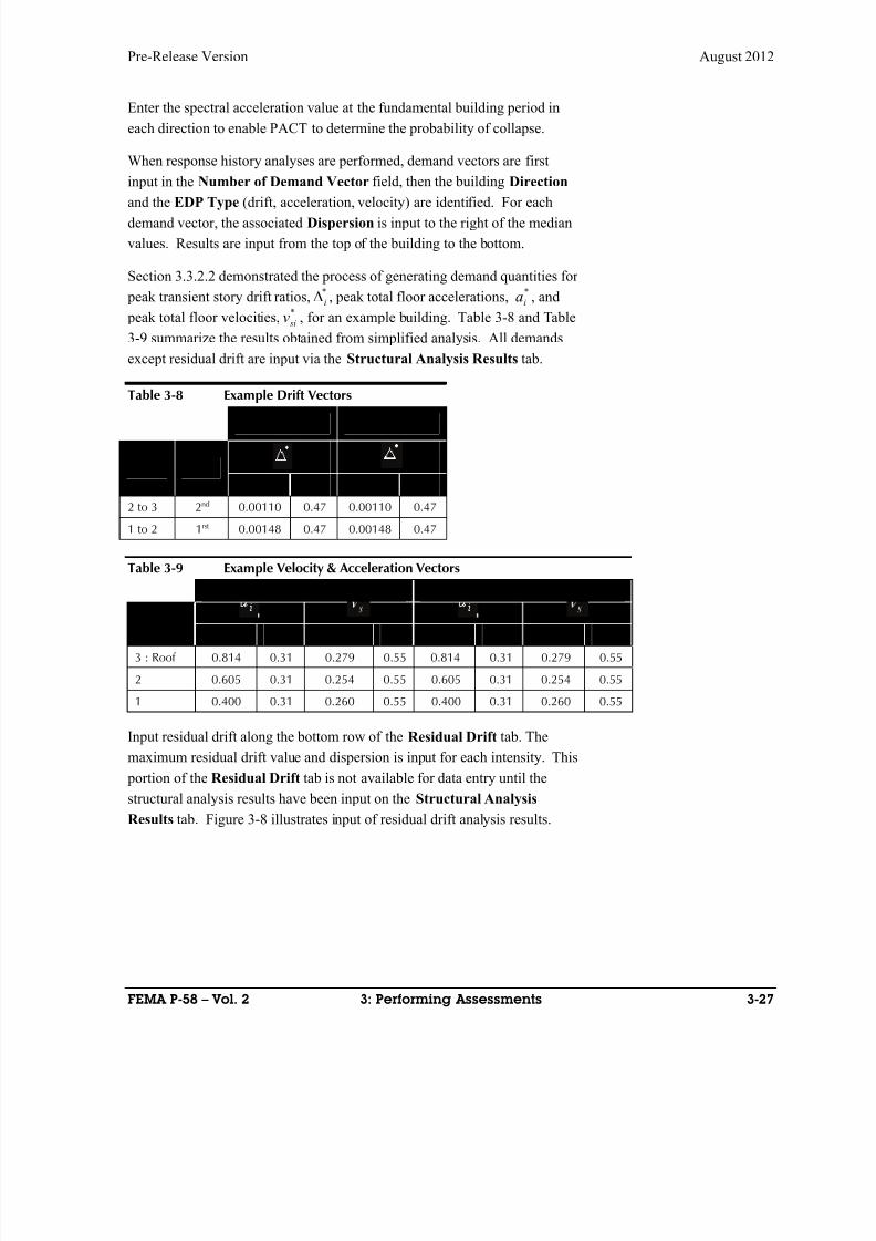
8/12/2019 Seismic Performance Assessment of Buildings
http://slidepdf.com/reader/full/seismic-performance-assessment-of-buildings 111/358
Pre-Release Version August 2012
FEMA P-58 – Vol. 2 3: Performing Assessments 3-27
Enter the spectral acceleration value at the fundamental building period in
each direction to enable PACT to determine the probability of collapse.
When response history analyses are performed, demand vectors are first
input in the Number of Demand Vector field, then the building Direction
and the EDP Type (drift, acceleration, velocity) are identified. For eachdemand vector, the associated Dispersion is input to the right of the median
values. Results are input from the top of the building to the bottom.
Section 3.3.2.2 demonstrated the process of generating demand quantities for
peak transient story drift ratios,*
i , peak total floor accelerations,*
ia , and
peak total floor velocities,*
siv , for an example building. Table 3-8 and Table
3-9 summarize the results obtained from simplified analysis. All demands
except residual drift are input via the Structural Analysis Results tab.
Table 3-8 Example Drift Vectors
Direction 1 Direction 2
Floor Story
θ β θ β
2 to 3 2nd 0.00110 0.47 0.00110 0.47
1 to 2 1rst 0.00148 0.47 0.00148 0.47
Table 3-9 Example Velocity & Acceleration Vectors
Direction 1 Direction 2
Floorθ β θ β θ β θ β
3 : Roof 0.814 0.31 0.279 0.55 0.814 0.31 0.279 0.55
2 0.605 0.31 0.254 0.55 0.605 0.31 0.254 0.55
1 0.400 0.31 0.260 0.55 0.400 0.31 0.260 0.55
Input residual drift along the bottom row of the Residual Drift tab. The
maximum residual drift value and dispersion is input for each intensity. This
portion of the Residual Drift tab is not available for data entry until the
structural analysis results have been input on the Structural Analysis
Results tab. Figure 3-8 illustrates input of residual drift analysis results.
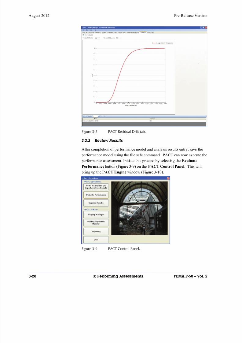
8/12/2019 Seismic Performance Assessment of Buildings
http://slidepdf.com/reader/full/seismic-performance-assessment-of-buildings 112/358
August 2012 Pre-Release Version
3-28 3: Performing Assessments FEMA P-58 – Vol. 2
Figure 3-8 PACT Residual Drift tab.
3.3.3 Review Results
After completion of performance model and analysis results entry, save the
performance model using the file safe command. PACT can now execute the
performance assessment. Initiate this process by selecting the Evaluate
Performance button (Figure 3-9) on the PACT Control Panel. This will
bring up the PACT Engine window (Figure 3-10).
Figure 3-9 PACT Control Panel.
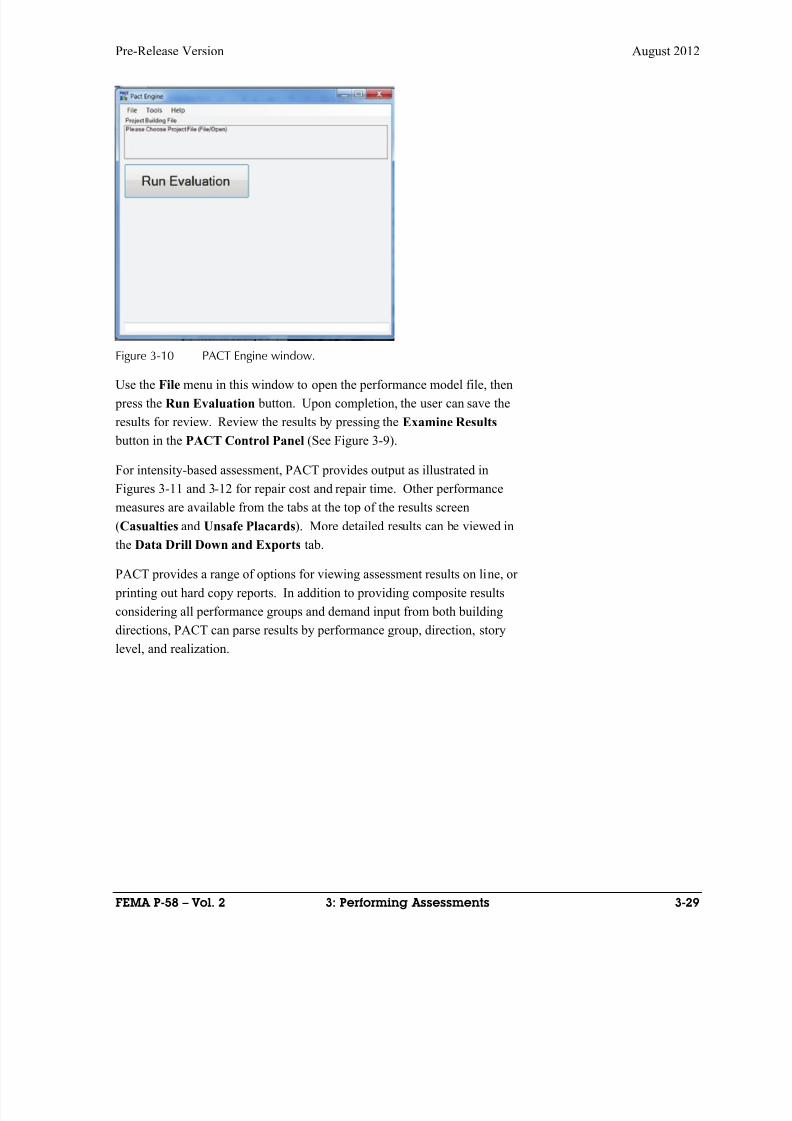
8/12/2019 Seismic Performance Assessment of Buildings
http://slidepdf.com/reader/full/seismic-performance-assessment-of-buildings 113/358
Pre-Release Version August 2012
FEMA P-58 – Vol. 2 3: Performing Assessments 3-29
Figure 3-10 PACT Engine window.
Use the File menu in this window to open the performance model file, then
press the Run Evaluation button. Upon completion, the user can save the
results for review. Review the results by pressing the Examine Results
button in the PACT Control Panel (See Figure 3-9).
For intensity-based assessment, PACT provides output as illustrated in
Figures 3-11 and 3-12 for repair cost and repair time. Other performance
measures are available from the tabs at the top of the results screen
(Casualties and Unsafe Placards). More detailed results can be viewed in
the Data Drill Down and Exports tab.
PACT provides a range of options for viewing assessment results on line, or
printing out hard copy reports. In addition to providing composite results
considering all performance groups and demand input from both building
directions, PACT can parse results by performance group, direction, story
level, and realization.
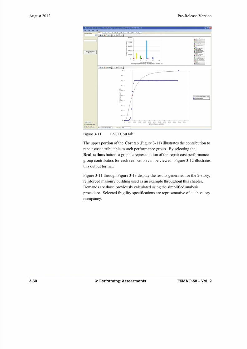
8/12/2019 Seismic Performance Assessment of Buildings
http://slidepdf.com/reader/full/seismic-performance-assessment-of-buildings 114/358
August 2012 Pre-Release Version
3-30 3: Performing Assessments FEMA P-58 – Vol. 2
Figure 3-11 PACT Cost tab.
The upper portion of the Cost tab (Figure 3-11) illustrates the contribution to
repair cost attributable to each performance group. By selecting the
Realizations button, a graphic representation of the repair cost performance
group contributors for each realization can be viewed. Figure 3-12 illustrates
this output format.
Figure 3-11 through Figure 3-13 display the results generated for the 2-story,
reinforced masonry building used as an example throughout this chapter.
Demands are those previously calculated using the simplified analysis
procedure. Selected fragility specifications are representative of a laboratory
occupancy.
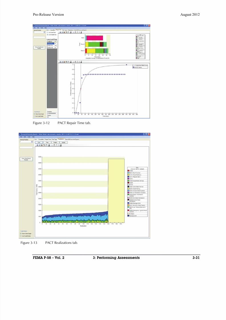
8/12/2019 Seismic Performance Assessment of Buildings
http://slidepdf.com/reader/full/seismic-performance-assessment-of-buildings 115/358
Pre-Release Version August 2012
FEMA P-58 – Vol. 2 3: Performing Assessments 3-31
Figure 3-12 PACT Repair Time tab.
Figure 3-13 PACT Realizations tab.
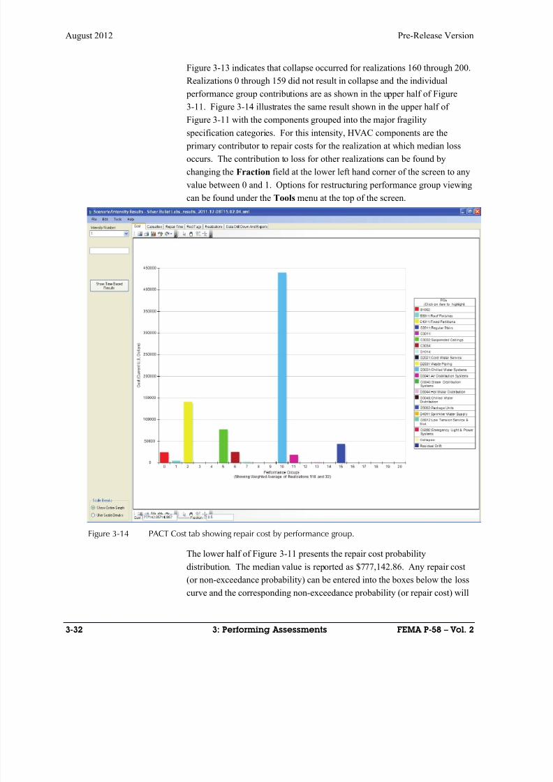
8/12/2019 Seismic Performance Assessment of Buildings
http://slidepdf.com/reader/full/seismic-performance-assessment-of-buildings 116/358
August 2012 Pre-Release Version
3-32 3: Performing Assessments FEMA P-58 – Vol. 2
Figure 3-13 indicates that collapse occurred for realizations 160 through 200.
Realizations 0 through 159 did not result in collapse and the individual
performance group contributions are as shown in the upper half of Figure
3-11. Figure 3-14 illustrates the same result shown in the upper half of
Figure 3-11 with the components grouped into the major fragility
specification categories. For this intensity, HVAC components are the
primary contributor to repair costs for the realization at which median loss
occurs. The contribution to loss for other realizations can be found by
changing the Fraction field at the lower left hand corner of the screen to any
value between 0 and 1. Options for restructuring performance group viewing
can be found under the Tools menu at the top of the screen.
Figure 3-14 PACT Cost tab showing repair cost by performance group.
The lower half of Figure 3-11 presents the repair cost probability
distribution. The median value is reported as $777,142.86. Any repair cost
(or non-exceedance probability) can be entered into the boxes below the loss
curve and the corresponding non-exceedance probability (or repair cost) will
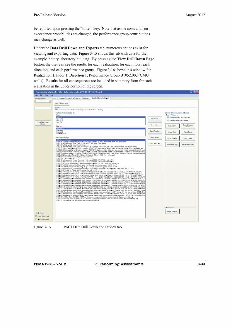
8/12/2019 Seismic Performance Assessment of Buildings
http://slidepdf.com/reader/full/seismic-performance-assessment-of-buildings 117/358
Pre-Release Version August 2012
FEMA P-58 – Vol. 2 3: Performing Assessments 3-33
be reported upon pressing the “Enter” key. Note that as the costs and non-
exceedance probabilities are changed, the performance group contributions
may change as well.
Under the Data Drill Down and Exports tab, numerous options exist for
viewing and exporting data. Figure 3-15 shows this tab with data for theexample 2 story laboratory building. By pressing the View Drill Down Page
button, the user can see the results for each realization, for each floor, each
direction, and each performance group. Figure 3-16 shows this window for
Realization 1, Floor 1, Direction 1, Performance Group B1052.003 (CMU
walls). Results for all consequences are included in summary form for each
realization in the upper portion of the screen.
Figure 3-15 PACT Data Drill Down and Exports tab.
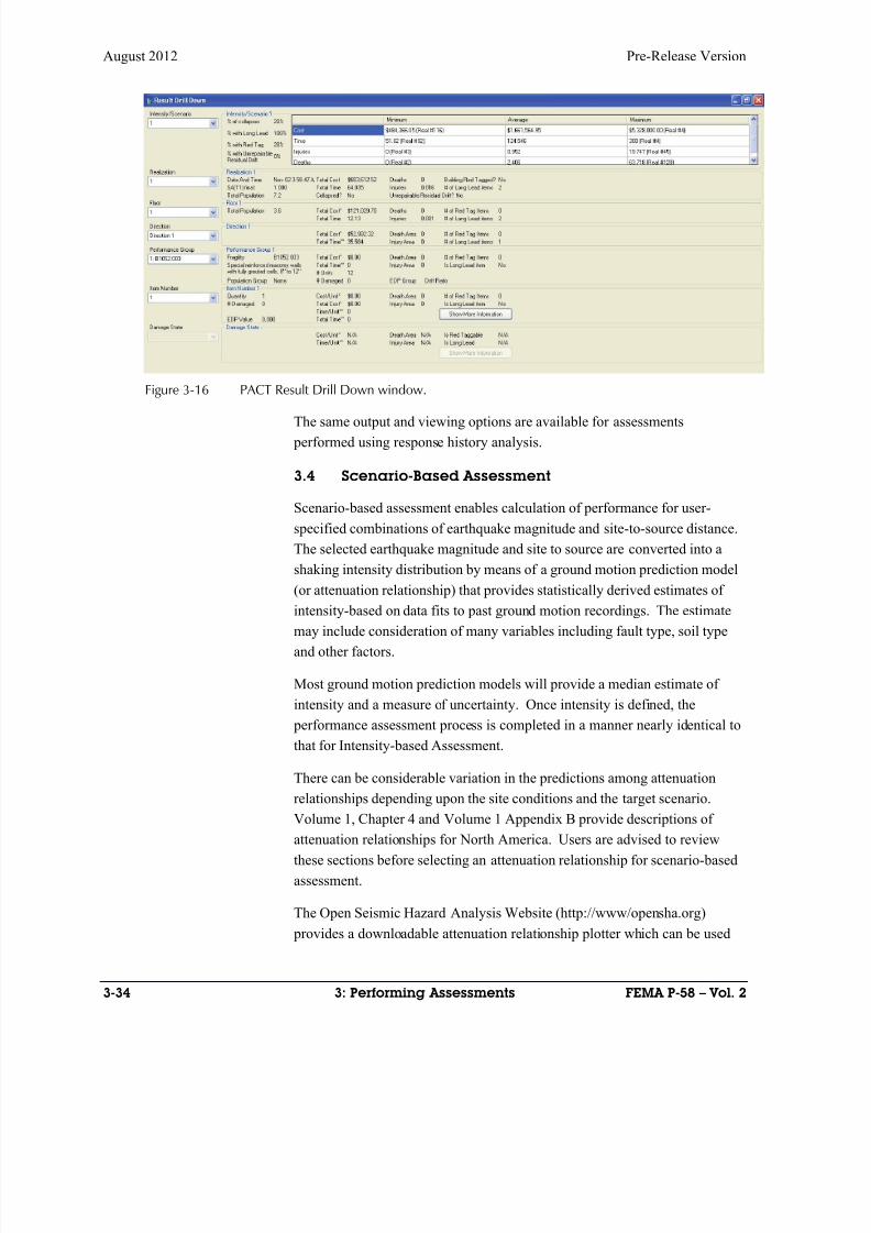
8/12/2019 Seismic Performance Assessment of Buildings
http://slidepdf.com/reader/full/seismic-performance-assessment-of-buildings 118/358
August 2012 Pre-Release Version
3-34 3: Performing Assessments FEMA P-58 – Vol. 2
Figure 3-16 PACT Result Drill Down window.
The same output and viewing options are available for assessments
performed using response history analysis.
3.4 Scenario-Based Assessment
Scenario-based assessment enables calculation of performance for user-
specified combinations of earthquake magnitude and site-to-source distance.
The selected earthquake magnitude and site to source are converted into a
shaking intensity distribution by means of a ground motion prediction model
(or attenuation relationship) that provides statistically derived estimates of
intensity-based on data fits to past ground motion recordings. The estimate
may include consideration of many variables including fault type, soil type
and other factors.
Most ground motion prediction models will provide a median estimate of
intensity and a measure of uncertainty. Once intensity is defined, the
performance assessment process is completed in a manner nearly identical to
that for Intensity-based Assessment.
There can be considerable variation in the predictions among attenuation
relationships depending upon the site conditions and the target scenario.
Volume 1, Chapter 4 and Volume 1 Appendix B provide descriptions of
attenuation relationships for North America. Users are advised to review
these sections before selecting an attenuation relationship for scenario-based
assessment.
The Open Seismic Hazard Analysis Website (http://www/opensha.org)
provides a downloadable attenuation relationship plotter which can be used
8/12/2019 Seismic Performance Assessment of Buildings
http://slidepdf.com/reader/full/seismic-performance-assessment-of-buildings 119/358
Pre-Release Version August 2012
FEMA P-58 – Vol. 2 3: Performing Assessments 3-35
to generate median spectra and dispersions for the following attenuation
relationships:
Boore and Atkinson
Campbell and Bozorgnia
Chiou and Youngs
Users can select any magnitude-distance pair they desire for assessment.
Some decision-makers will be interested in a building’s performance if a
repeat occurrence of a historic event occurs. Parameters defining many
historic events are available from numerous sources including searchable
catalogs at http://earthquake.usgs.gov/research/data?areaID=13.
Some decision-makers may desire performance assessments for worst-case
scenarios. The USGS posts information on best estimate maximum
magnitudes for active faults in the Western US and the Inner Mountainseismic region at http://earthquake.usgs.gov/hazards/qfaults/.
3.4.1 Nonlinear Response-History Analysis
3.4.1.1 Define Earthquake Hazards
Volume 1 presents two procedures for ground motion generation for use in
scenario-based assessment.
In the first procedure, ground motions are selected and scaled to a median
spectrum obtained from the ground motion prediction model and prediction
model uncertainty obtained from the model is assigned as an additionalcomponent of total dispersion. This procedure involves the following steps:
Step 1. Determine the building’s fundamental translation periods in each of
two principal directions, T 1 x, .
Step 2. Determine the average first mode period T as the average of T 1 x and
T 1 y if the mode shapes are uncoupled and as the larger of T 1
x or T 1 y if the
mode shapes are coupled.
Step 3. Estimate the average wave velocity, V s30, in the upper 30 meters (100
ft.) of soil at the site.
Step 4. Select an appropriate attenuation relationship that best matches the
fault characteristics, regional geology and site conditions for the scenario
event and building site. Downloadable attenuation functions are available at
http://www.opensha.org.
8/12/2019 Seismic Performance Assessment of Buildings
http://slidepdf.com/reader/full/seismic-performance-assessment-of-buildings 120/358
August 2012 Pre-Release Version
3-36 3: Performing Assessments FEMA P-58 – Vol. 2
Step 5. Determine the values of variables used in the selected attenuation
relationship.
Step 6. Use the attenuation relationship to generate the median value of
spectral acceleration and associated period dependent dispersion over the full
range of potential structural periods (0.01 to 5 seconds).
Step 7. If the attenuation relationship does not include consideration of site
characteristics and class, adjust the spectrum to account for these effects,
using site response analysis, site class coefficients contained in ASCE 7 or
other suitable adjustment factors.
Step 8. Calculate the structural period range of interest for spectral scaling
as:
min 0.2T T
max 2.0T T
Step 9. Select n ground motion pairs with 5% damped geomean spectral
shape similar to the spectrum generated in steps 6 and 7 over the period
range T min to T max.
Step 10. Amplitude scale the suite of records to match the target spectrum.
In the second procedure, ground motions are selected to represent the
dispersion in intensity obtained from the ground motion prediction model.
Volume 1 Appendix B, Section B.7 presents this second procedure.
Section 3.4.2 illustrates the use of an attenuation relationship to generate an
elastic response spectrum characterization of ground shaking. Chapter 5
provides an example application illustrating ground motion selection and
scaling to a target spectrum. For a scenario-based assessment, selection and
scaling of ground motion is done to match the spectrum generated from the
attenuation relationship.
3.4.1.2 Analyze Building Response
Per Section 3.4.1.1, n analyses using the n scaled ground motion pairs are
performed. Median values and dispersions for peak transient drift, peak flooracceleration and residual drift are obtained from the following steps:
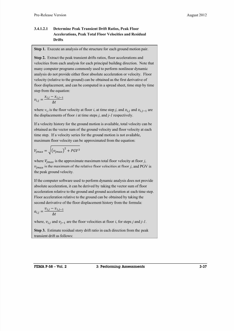
8/12/2019 Seismic Performance Assessment of Buildings
http://slidepdf.com/reader/full/seismic-performance-assessment-of-buildings 121/358
Pre-Release Version August 2012
FEMA P-58 – Vol. 2 3: Performing Assessments 3-37
3.4.1.2.1 Determine Peak Transient Drift Ratios, Peak Floor
Accelerations, Peak Total Floor Velocities and Residual
Drifts
Step 1. Execute an analysis of the structure for each ground motion pair.
Step 2. Extract the peak transient drifts ratios, floor accelerations and
velocities from each analysis for each principal building direction. Note that
many computer programs commonly used to perform nonlinear dynamic
analysis do not provide either floor absolute acceleration or velocity. Floor
velocity (relative to the ground) can be obtained as the first derivative of
floor displacement, and can be computed in a spread sheet, time step by time
step from the equation:
, , ,∆
where vi,j is the floor velocity at floor i, at time step j, and , and , are
the displacements of floor i at time steps j, and j-1 respectively.
If a velocity history for the ground motion is available, total velocity can be
obtained as the vector sum of the ground velocity and floor velocity at each
time step. If a velocity series for the ground motion is not available,
maximum floor velocity can be approximated from the equation:
where is the approximate maximum total floor velocity at floor j, is the maximum of the relative floor velocities at floor j, and PGV is
the peak ground velocity.
If the computer software used to perform dynamic analysis does not provide
absolute acceleration, it can be derived by taking the vector sum of floor
acceleration relative to the ground and ground acceleration at each time step.
Floor acceleration relative to the ground can be obtained by taking the
second derivative of the floor displacement history from the formula:
, , ,
∆
where, , and are the floor velocities at floor i, for steps j and j-1.
Step 3. Estimate residual story drift ratio in each direction from the peak
transient drift as follows:
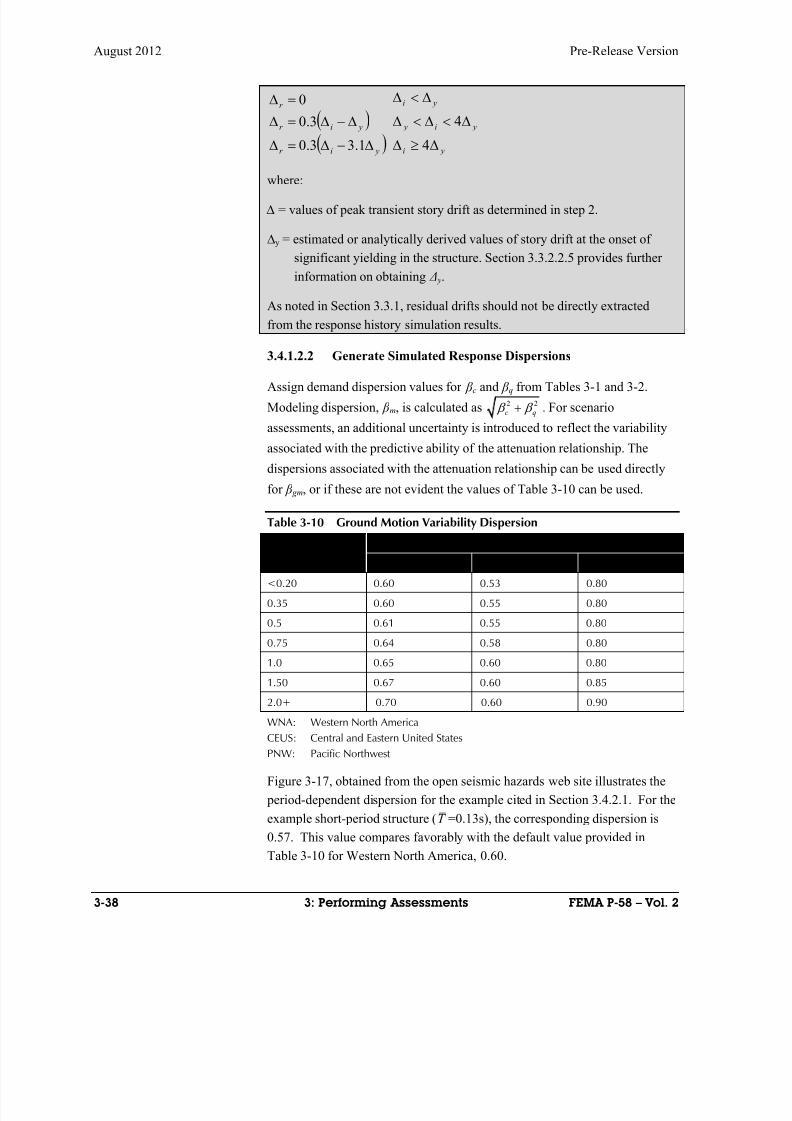
8/12/2019 Seismic Performance Assessment of Buildings
http://slidepdf.com/reader/full/seismic-performance-assessment-of-buildings 122/358
August 2012 Pre-Release Version
3-38 3: Performing Assessments FEMA P-58 – Vol. 2
yir
yir
r
1.33.0
3.0
0
yi
yi y
yi
4
4
where:
∆ = values of peak transient story drift as determined in step 2.
∆y = estimated or analytically derived values of story drift at the onset of
significant yielding in the structure. Section 3.3.2.2.5 provides further
information on obtaining Δ y.
As noted in Section 3.3.1, residual drifts should not be directly extracted
from the response history simulation results.
3.4.1.2.2 Generate Simulated Response Dispersions
Assign demand dispersion values for β c and β q from Tables 3-1 and 3-2.
Modeling dispersion, β m, is calculated as 2 2
c q . For scenario
assessments, an additional uncertainty is introduced to reflect the variability
associated with the predictive ability of the attenuation relationship. The
dispersions associated with the attenuation relationship can be used directly
for β gm, or if these are not evident the values of Table 3-10 can be used.
Table 3-10 Ground Motion Variability Dispersion
T 1 (sec) β gm
WNA CEUS PNW
<0.20 0.60 0.53 0.80
0.35 0.60 0.55 0.80
0.5 0.61 0.55 0.80
0.75 0.64 0.58 0.80
1.0 0.65 0.60 0.80
1.50 0.67 0.60 0.85
2.0+ 0.70 0.60 0.90
WNA: Western North America
CEUS: Central and Eastern United StatesPNW: Pacific Northwest
Figure 3-17, obtained from the open seismic hazards web site illustrates the
period-dependent dispersion for the example cited in Section 3.4.2.1. For the
example short-period structure (T =0.13s), the corresponding dispersion is
0.57. This value compares favorably with the default value provided in
Table 3-10 for Western North America, 0.60.

8/12/2019 Seismic Performance Assessment of Buildings
http://slidepdf.com/reader/full/seismic-performance-assessment-of-buildings 123/358
Pre-Release Version August 2012
FEMA P-58 – Vol. 2 3: Performing Assessments 3-39
Combine the ground motion dispersion β gm with β c and β q to produce β m for
use in scenario assessments as:
2 22
m c q gm
Figure 3-17 Standard deviation of Sa vs T attenuation plot fromwww.opensha.org.
If the alternate procedures for scaling ground motion records are used for
analysis, β gm need not be included in the total assigned dispersion since itseffects have been captured directly in the calculation process.
3.4.1.3 Input Response and Calculate Performance
Enter structural analysis results into PACT in a manner similar to that for
intensity-based assessment. Figure 3-18 illustrates the input for direction 1
drift values from analyses performed with 7 ground motion pairs scaled to
the scenario target spectrum. The modeling dispersion β m includes the β gm
variability term.
Figure 3-18 PACT Structural Analysis Results tab.
8/12/2019 Seismic Performance Assessment of Buildings
http://slidepdf.com/reader/full/seismic-performance-assessment-of-buildings 124/358
August 2012 Pre-Release Version
3-40 3: Performing Assessments FEMA P-58 – Vol. 2
3.4.2 Simplified Analysis
3.4.2.1 Define Earthquake Hazards
The simplified analysis method of requires spectral response accelerations
obtained from a 5% damped elastic response spectrum consistent with the
selected magnitude and distance scenario. This requires selection and use ofa ground motion prediction model to define the scenario response spectrum.
Volume 1 Chapter 5 and Volume 1 Appendix B provide information on
selection and use of these models, often termed attenuation relationships.
The basic steps are illustrated below:
The 2-story reinforced masonry wall building previously used to illustrate the
simplified analysis approach for intensity-based assessment. Assumed
conditions are:
Site Soil Class D
Distance to fault (closest horizontal distance to the vertical projection of
rupture) = r jb = 20 km
Earthquake magnitude, M w = 6.5
Fault type: Strike-slip
Step 1. Estimate the average shear wave velocity (V s30) in the upper 30
meters (100 ft.) of site soils.
sm s ft V S /8.243/80030
Step 2. Select an appropriate attenuation relationship that best matches thefault characteristics, regional geology and site conditions of the scenario
event and the reference building site.
Boore & Atkinson (2008) function is selected on the attenuation relationship
application available at http://www.opensha.org, and the above data are
input. Figures 3-17 and 3-19 indicate the median prediction for S a and the
associated dispersion, both as a function of period T .
Step 3. Define the value of variables used in the selected attenuation
relationship.
From previous analysis, T 1x = T 1y = 0.13seconds.
Step 4. Use the attenuation relationship to generate the median value of
spectral acceleration and associated period dependent dispersion over the full
range of potential structural periods (0.01 to 5 seconds), to derive the
estimated median response spectrum (Figure 3-19).
8/12/2019 Seismic Performance Assessment of Buildings
http://slidepdf.com/reader/full/seismic-performance-assessment-of-buildings 125/358
Pre-Release Version August 2012
FEMA P-58 – Vol. 2 3: Performing Assessments 3-41
From the Boore & Atkinson (2008) plot, S a(0.13s) = 0.177g for both X and Y
directions. The corresponding dispersion is 0.57.
Step 5. If the attenuation relationship does not include consideration of site
characteristics and class, adjust the spectrum to account for these effects,
using site response analysis, site class coefficients contained in ASCE 7 orother suitable adjustment factors.
Attenuation relationships generally return spectral acceleration values that
reflect a geomean ( gmS ) of horizontal components (S ax, S ay), where:
gm ax aY S S S
The simplified analysis approach requires application of a spectral
acceleration ordinate along each principal building axis. To convert the
geomean spectrum to a pair of spectral ordinates oriented along each
principal building axis, the process is as follows:
Determine periods T 1x and T 1y.
Using the response spectrum derived as described above, determine
1
xaS T and 1
yaS T .
For simplified analysis both the value of spectral acceleration at the
structure’s effective first mode period S a(0.13) and the peak ground
acceleration, S a(0), are needed. These values can be obtained from the plot
shown in Figure 3-18 or by re-executing the software for peak ground
acceleration as an intensity measure in lieu of S a.
For predictions of peak total floor velocity, a median estimate of the peak
ground velocity is needed. The Boore & Atkinson (2008) attenuation
function will return median estimates and dispersions for this intensity
measure in a fashion similar to that for peak ground acceleration.
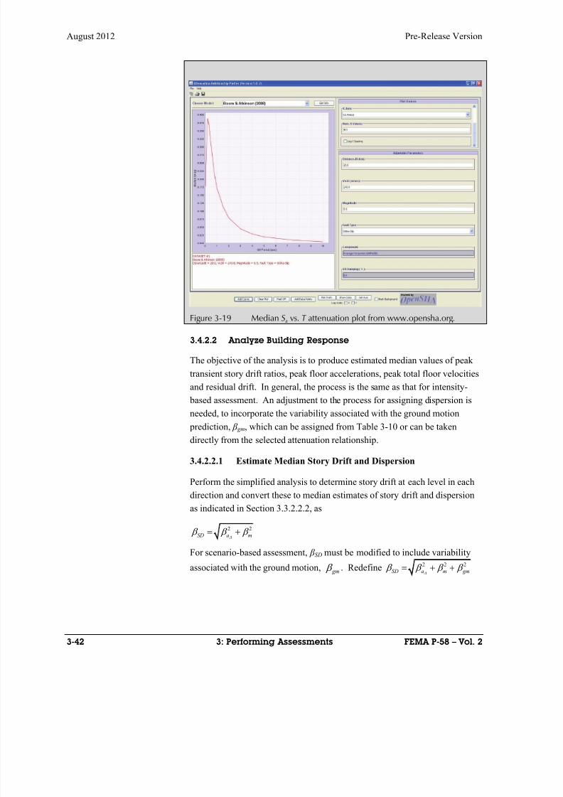
8/12/2019 Seismic Performance Assessment of Buildings
http://slidepdf.com/reader/full/seismic-performance-assessment-of-buildings 126/358
August 2012 Pre-Release Version
3-42 3: Performing Assessments FEMA P-58 – Vol. 2
Figure 3-19 Median Sa vs. T attenuation plot from www.opensha.org.
3.4.2.2 Analyze Building Response
The objective of the analysis is to produce estimated median values of peak
transient story drift ratios, peak floor accelerations, peak total floor velocities
and residual drift. In general, the process is the same as that for intensity-
based assessment. An adjustment to the process for assigning dispersion is
needed, to incorporate the variability associated with the ground motion
prediction, β gm, which can be assigned from Table 3-10 or can be taken
directly from the selected attenuation relationship.
3.4.2.2.1 Estimate Median Story Drift and Dispersion
Perform the simplified analysis to determine story drift at each level in each
direction and convert these to median estimates of story drift and dispersion
as indicated in Section 3.3.2.2.2, as
2 2
SD a m
For scenario-based assessment, β SD must be modified to include variability
associated with the ground motion, gm . Redefine 2 2 2
SD a m gm

8/12/2019 Seismic Performance Assessment of Buildings
http://slidepdf.com/reader/full/seismic-performance-assessment-of-buildings 127/358
Pre-Release Version August 2012
FEMA P-58 – Vol. 2 3: Performing Assessments 3-43
3.4.2.2.2 Estimate Median Peak Floor Acceleration and Dispersion
Section 3.3.2.2.3 describes the process for estimating median peak floor
acceleration at each level. The equation to calculate floor acceleration
dispersion β FA is modified as follows:
222
gmmaa FA
where gm is the dispersion associated with the ground motion.
3.4.2.2.3 Estimate Median Peak Total Floor Velocity and Dispersion
Determine estimated median peak floor velocity and dispersion as described
in Section 3.3.2.2.4.
The equation used to calculate FV is modified: as follows
222 gmmav FV
where gm is defined above.
3.4.2.2.4 Estimate Median Residual Story Drift and Dispersion
Refer to Section 3.3.2.2.5 for calculation of residual story drift. 0.8 RD is
to be used for intensity or scenario-based assessments.
3.4.2.3 Input Response and Calculate Performance
Demand vectors and dispersions are organized and entered into PACT in a
similar fashion as that described for intensity assessments. See Section
3.3.2.3. Note that gm is incorporated into the total dispersion assigned to
the median demand values. Figure 3-20 illustrates the Structural Analysis
Results tab for the simplified analysis approach in scenario-based
assessment.
Figure 3-20 PACT Structural Analysis Results tab.
8/12/2019 Seismic Performance Assessment of Buildings
http://slidepdf.com/reader/full/seismic-performance-assessment-of-buildings 128/358
August 2012 Pre-Release Version
3-44 3: Performing Assessments FEMA P-58 – Vol. 2
3.4.3 Review Results
The PACT assessment results for scenario-based assessment are similar to
those produced for intensity-based assessment as illustrated in Section 3.3.
3.5 Time-Based Assessment
Time-based assessments express the probability of incurring impacts over a
period of time, considering all earthquakes that occur in that time and the
probability that they could occur. A site seismic hazard curve is used to
express the annual frequency of exceedance for the values of a selected
ground motion parameter. Ground motion parameters of interest for the
assessment methodology include spectral acceleration at the average
fundamental period of the building, peak ground acceleration and peak
ground velocity.
The time-based assessment process consists of a sequence of intensity-basedassessments that span the range of potential seismic hazards from the lowest
seismic intensity that can result in meaningful loss to the upper limits of
intensity where total loss is highly probable. The process is performed by
dividing the seismic hazard curve into a number of equal segments (eight
segments are recommended). From each segment, a central value of spectral
acceleration is selected. The building is analyzed for each intensity and a
performance assessment is executed factoring the loss in each segment by the
probability of occurrence associated with the intensities in the segment. The
resulting curves express the annual exceedance frequency for the various
performance measures. The sections that follow detail the steps in this process.
3.5.1. Nonlinear Response-History Analysis
3.5.1.1 Define Earthquake Hazards
For time-based assessments, nonlinear response-history analyses are
conducted for m sets of n ground motion pairs each, scaled to appropriate
intensity values using the procedures of Volume 1, Chapter 4. A value of m
= 8 is recommended. For very weak buildings m can be taken smaller than 8.
For highly resistant buildings, it may be necessary to increase the number of
segments or increase the range of segments to obtain stable results.
Generate ground motion records for time-based assessments as follows:
Step 1. Determine the building’s fundamental translational periods in two
orthogonal directions (T 1 x and T 1
y).

8/12/2019 Seismic Performance Assessment of Buildings
http://slidepdf.com/reader/full/seismic-performance-assessment-of-buildings 129/358
Pre-Release Version August 2012
FEMA P-58 – Vol. 2 3: Performing Assessments 3-45
Step 2. Determine the average first mode period T as the average of T 1 x and
T 1 y if the mode shapes are uncoupled and as the larger of T 1
x and T 1 y if the
mode shapes are coupled.
Step 3. Generate a seismic hazard curve for the site for S a. This can be
done by performing a site specific seismic hazard analysis or using hazarddata compiled by USGS.
Step 4. Define values of S a min and S a max that span the range of
interest for the building. S a min should reflect the onset of non-trivial
impacts and, can be taken as follows:
for ≤ 1.0s
for > 1.0s
Similarly, S a max should reflect a maximum value for the selected
performance measures and can be taken as:
S a max= 2 S a where S a is evaluated at annual frequency of
exceedance, λ =0.0004 but need not exceed Ŝ a (T ), the building’s median
collapse capacity. Section 2.6 provides guidance on estimating median
collapse capacity.
Step 5. Divide the seismic hazard curve into an appropriate number of
intensity segments that span the range of from S a min to S a max .
Step 6. For each segment defined in Step 5, identify the value at themidpoint of the segment and the Mean Annual Frequencies of Exceedance at
each segment end. The difference between mean annual exceedance
frequency values at the segment ends defines the segment annual occurrence
frequency ∆λi.
Step 7. Develop an appropriate response spectrum for each of the
and ∆λi. Refer to Appendix B, Volume 1 for information on generation of
various types of spectra. For events with a relatively large occurrence
frequency both uniform hazard and conditional mean spectra should have
similar shape and are appropriate for use. For small occurrence frequency(infrequent) events, use of conditional mean or conditional spectra should
improve estimates of drifts and accelerations over those generated using
uniform hazard spectra.
Step 8. Select and scale ground motion pairs to the amplitude of the target
spectrum at the S a(T ) value similar to process for intensity-based
assessment. Ground motion record pairs can be found at:
min( ) 0.05aS T g T
min
0.05( )aS T g
T T
( )iaS T
( )iaS T

8/12/2019 Seismic Performance Assessment of Buildings
http://slidepdf.com/reader/full/seismic-performance-assessment-of-buildings 130/358
August 2012 Pre-Release Version
3-46 3: Performing Assessments FEMA P-58 – Vol. 2
www.peer.berkeley.edu and www.cosmos-eq.org. A minimum of 7 record
pairs with geomean spectral shape similar to the target spectrum should be
used. If records with appropriate spectral shape cannot be found, at least 11
record pairs should be used.
Step 9. Repeat Step 8 for each hazard curve segment to obtain scaledrecords for the full range of the segments.
Chapter 5 illustrates execution of Step 1 through Step 9 for a 4-story
reinforced concrete frame structure. Section 3.5.2.1 illustrates steps 1
through 6.
3.5.1.2 Analyze Building Response
Analyze the structure with the selected records for each spectral intensity
segment. Extract the peak transient drift ratios, floor accelerations, and peak
total floor velocities for each of the orthogonal building directions. Calculate
residual drift ratio and demand dispersions in the same manner as for
intensity-based assessment. See Section 3.3.1.2.
For spectral intensities that approach the structure’s median collapse capacity
, some ground motion pairs may produce predictions of collapse.
Discard the results for analyses that produce collapse. In this case, additional
analyses may be need. Section 3.3.1.2 and Section 5.8 provide further
guidance on this.
3.5.1.3 Input Response and Calculate Performance
For time-based assessments, PACT requires input of n demand vectors for
each intensity assessment. Nonlinear response-history analysis may produce
a different number of demand vectors for each spectral segment due to
occurrence of collapse for some records. Response vectors should include
values for each demand parameter utilized by the selected component
fragility specifications.
Chapter 5 illustrates inputting structural analysis results for one intensity
level of a 4-story reinforced concrete frame structure. The structural analysis
results for each intensity segment are input similarly. Information defining
the mean annual frequency values of each intensity segment is input on thePACT Hazard Curve tab.
3.5.2 Simplified Analysis
3.5.2.1 Define Earthquake Hazards
Ground shaking effects are characterized by spectral ordinates extracted from
a seismic hazard curve that spans the anticipated range of meaningful
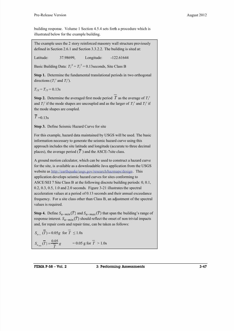
8/12/2019 Seismic Performance Assessment of Buildings
http://slidepdf.com/reader/full/seismic-performance-assessment-of-buildings 131/358
Pre-Release Version August 2012
FEMA P-58 – Vol. 2 3: Performing Assessments 3-47
building response. Volume 1 Section 4.5.4 sets forth a procedure which is
illustrated below for the example building.
The example uses the 2 story reinforced masonry wall structure previously
defined in Section 2.6.1 and Section 3.3.2.2. The building is sited at:
Latitude: 37.98699, Longitude: -122.61644
Basic Building Data: T 1 X = T 1
Y = 0.13seconds, Site Class B
Step 1. Determine the fundamental translational periods in two orthogonal
directions (T 1 x and T 1
y).
T 1X = T 1Y = 0.13s
Step 2. Determine the averaged first mode period T as the average of T 1 x
and T 1 y if the mode shapes are uncoupled and as the larger of T 1
x and T 1 y if
the mode shapes are coupled.
T =0.13s
Step 3. Define Seismic Hazard Curve for site
For this example, hazard data maintained by USGS will be used. The basic
information necessary to generate the seismic hazard curve using this
approach includes the site latitude and longitude (accurate to three decimal
places), the average period (T ) and the ASCE-7site class.
A ground motion calculator, which can be used to construct a hazard curve
for the site, is available as a downloadable Java application from the USGS
website as http://earthquake/usgs.gov/research/hazmaps/design. This
application develops seismic hazard curves for sites conforming to
ASCE/SEI 7 Site Class B at the following discrete building periods: 0, 0.1,
0.2, 0.3, 0.5, 1.0 and 2.0 seconds. Figure 3-21 illustrates the spectral
acceleration values at a period of 0.13 seconds and their annual exceedance
frequency. For a site class other than Class B, an adjustment of the spectral
values is required.
Step 4. Define
and
that span the building’s range of
response interest. should reflect the onset of non trivial impacts
and, for repair costs and repair time, can be taken as follows:
for ≤ 1.0s
= 0.05 g for > 1.0s
( ) 0.05aS T g T
min
0.05( )aS T g
T T
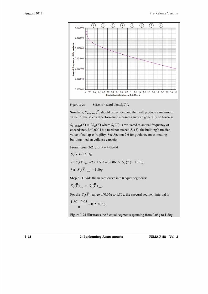
8/12/2019 Seismic Performance Assessment of Buildings
http://slidepdf.com/reader/full/seismic-performance-assessment-of-buildings 132/358
August 2012 Pre-Release Version
3-48 3: Performing Assessments FEMA P-58 – Vol. 2
Figure 3-21 Seismic hazard plot, Sa(T ).
Similarly, should reflect demand that will produce a maximum
value for the selected performance measures and can generally be taken as:
2 where is evaluated at annual frequency of
exceedance, λ =0.0004 but need not exceed Ŝ a (T ), the building’s median
value of collapse fragility. See Section 2.6 for guidance on estimating
building median collapse capacity.
From Figure 3-21, for λ = 4.0E-04
)(T S a =1.503g
max)(2 T S a =2 x 1.503 = 3.006g > g T S a 80.1)(ˆ
maxSet ( )aS T = 1.80 g
Step 5. Divide the hazard curve into 8 equal segments:
min)(T S a to max)(T S a .
For the )(T S a range of 0.05g to 1.80g, the spectral segment interval is
g 21875.08
05.080.1
Figure 3-21 illustrates the 8 equal segments spanning from 0.05g to 1.80g.
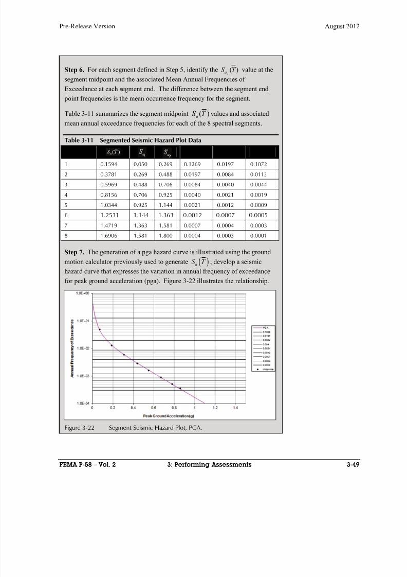
8/12/2019 Seismic Performance Assessment of Buildings
http://slidepdf.com/reader/full/seismic-performance-assessment-of-buildings 133/358
Pre-Release Version August 2012
FEMA P-58 – Vol. 2 3: Performing Assessments 3-49
Step 6. For each segment defined in Step 5, identify the value at the
segment midpoint and the associated Mean Annual Frequencies of
Exceedance at each segment end. The difference between the segment end
point frequencies is the mean occurrence frequency for the segment.
Table 3-11 summarizes the segment midpoint )(T S a values and associated
mean annual exceedance frequencies for each of the 8 spectral segments.
Table 3-11 Segmented Seismic Hazard Plot Data
Segment λi λ j Δλ
1 0.1594 0.050 0.269 0.1269 0.0197 0.1072
2 0.3781 0.269 0.488 0.0197 0.0084 0.0113
3 0.5969 0.488 0.706 0.0084 0.0040 0.0044
4 0.8156 0.706 0.925 0.0040 0.0021 0.0019
5 1.0344 0.925 1.144 0.0021 0.0012 0.0009
6 1.2531 1.144 1.363 0.0012 0.0007 0.0005
7 1.4719 1.363 1.581 0.0007 0.0004 0.0003
8 1.6906 1.581 1.800 0.0004 0.0003 0.0001
Step 7. The generation of a pga hazard curve is illustrated using the ground
motion calculator previously used to generate aS T , develop a seismic
hazard curve that expresses the variation in annual frequency of exceedance
for peak ground acceleration (pga). Figure 3-22 illustrates the relationship.
Figure 3-22 Segment Seismic Hazard Plot, PGA.
( )iaS T
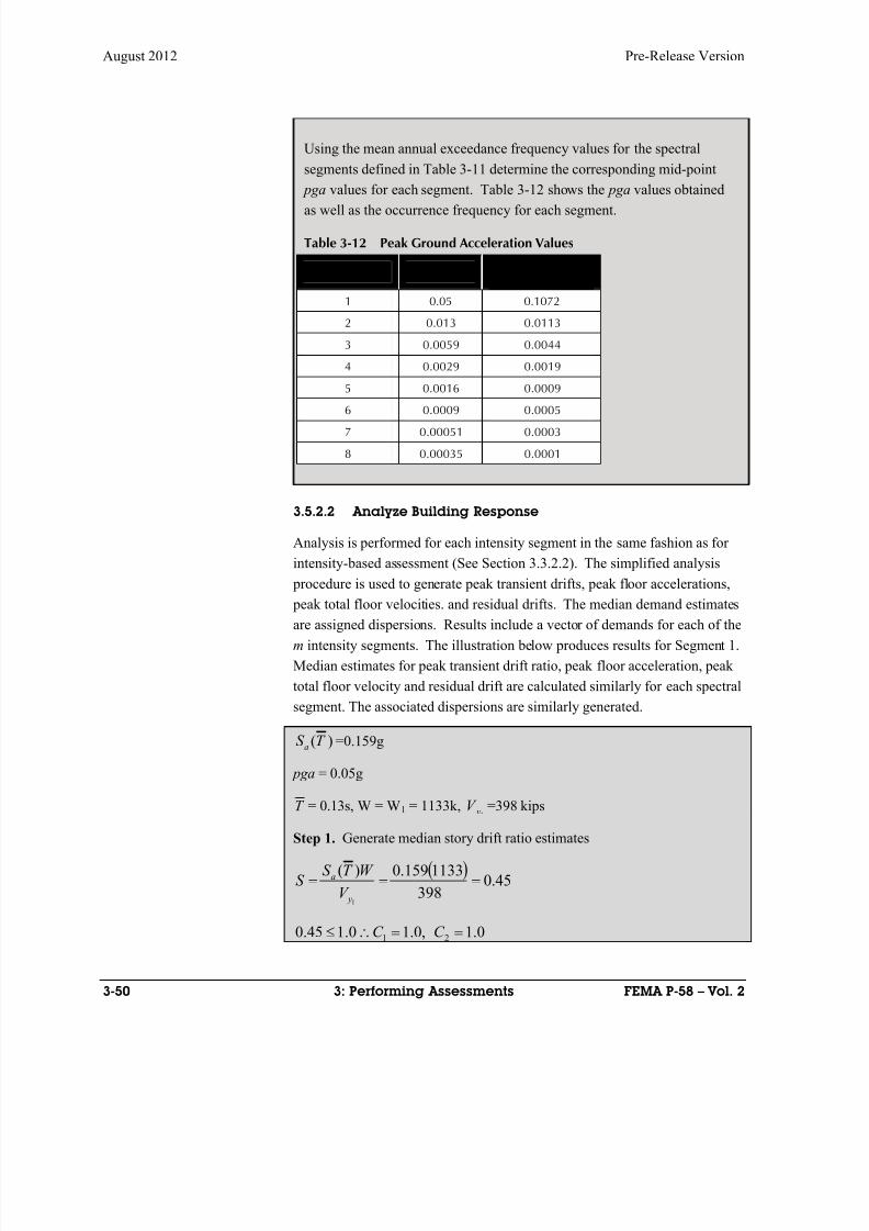
8/12/2019 Seismic Performance Assessment of Buildings
http://slidepdf.com/reader/full/seismic-performance-assessment-of-buildings 134/358
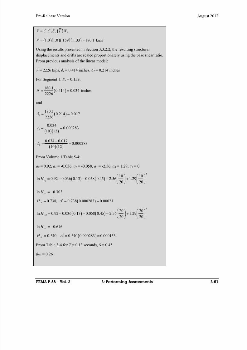
8/12/2019 Seismic Performance Assessment of Buildings
http://slidepdf.com/reader/full/seismic-performance-assessment-of-buildings 135/358
Pre-Release Version August 2012
FEMA P-58 – Vol. 2 3: Performing Assessments 3-51
1 2 1aV C C S T W
1.0 1.0 .159 1133 180.1 kipsV
Using the results presented in Section 3.3.2.2, the resulting structural
displacements and drifts are scaled proportionately using the base shear ratio.
From previous analysis of the linear model:
V = 2226 kips, δr = 0.414 inches, δ2 = 0.214 inches
For Segment 1: S a = 0.159,
180.1
0.414 0.034 inches2226
r
and
2
180.1
0.214 0.0172226
1
0.0340.000283
10 12
2
0.034 0.0170.000283
10 12
From Volume 1 Table 5-4:
a0 = 0.92, a1 = -0.036, a2 = -0.058, a3 = -2.56, a4 = 1.29, a5 = 0
1
210 10
ln 0.92 0.036 0.13 0.058 0.45 2.56 1.2920 20
H
1ln 0.303 H
1
*
10.738, 0.738 0.000283 0.00021 H
2
2
20 20ln 0.92 0.036 0.13 0.058 0.45 2.56 1.29
20 20 H
2
ln 0.616 H
2
*
20.540, 0.540 0.000283 0.000153 H
From Table 3-4 for T = 0.13 seconds, S = 0.45
β SD = 0.26
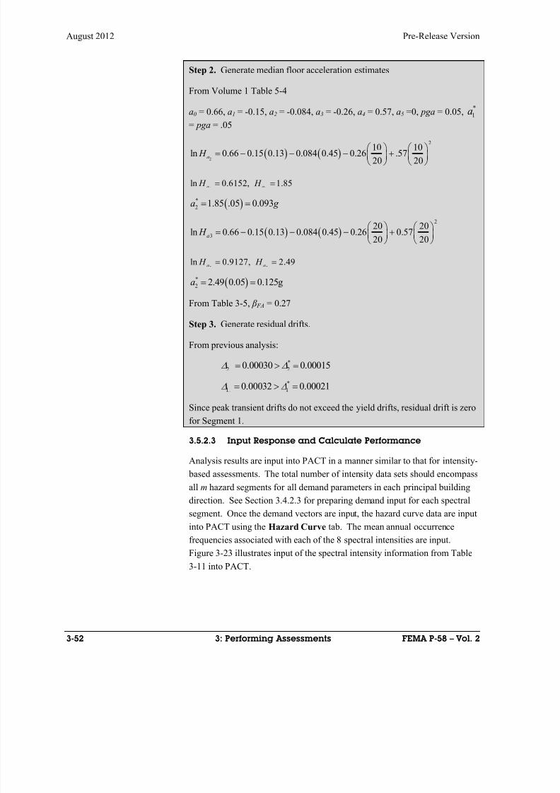
8/12/2019 Seismic Performance Assessment of Buildings
http://slidepdf.com/reader/full/seismic-performance-assessment-of-buildings 136/358
August 2012 Pre-Release Version
3-52 3: Performing Assessments FEMA P-58 – Vol. 2
Step 2. Generate median floor acceleration estimates
From Volume 1 Table 5-4
a0 = 0.66, a1 = -0.15, a2 = -0.084, a3 = -0.26, a4 = 0.57, a5 =0, pga = 0.05,*
1a
= pga = .05
2
210 10
ln 0.66 0.15 0.13 0.084 0.45 0.26 .5720 20
a H
2 2ln 0.6152, 1.85a a H H
*
2 1.85 .05 0.093a g
2
3
20 20ln 0.66 0.15 0.13 0.084 0.45 0.26 0.57
20 20a H
2 2ln 0.9127, 2.49a a H H
*
2 2.49 0.05 0.125ga
From Table 3-5, β FA = 0.27
Step 3. Generate residual drifts.
From previous analysis:
*
2 20.00030 0.00015 y
*
1 10.00032 0.00021 y
Since peak transient drifts do not exceed the yield drifts, residual drift is zero
for Segment 1.
3.5.2.3 Input Response and Calculate Performance
Analysis results are input into PACT in a manner similar to that for intensity-
based assessments. The total number of intensity data sets should encompass
all m hazard segments for all demand parameters in each principal building
direction. See Section 3.4.2.3 for preparing demand input for each spectral
segment. Once the demand vectors are input, the hazard curve data are input
into PACT using the Hazard Curve tab. The mean annual occurrence
frequencies associated with each of the 8 spectral intensities are input.
Figure 3-23 illustrates input of the spectral intensity information from Table
3-11 into PACT.

8/12/2019 Seismic Performance Assessment of Buildings
http://slidepdf.com/reader/full/seismic-performance-assessment-of-buildings 137/358
Pre-Release Version August 2012
FEMA P-58 – Vol. 2 3: Performing Assessments 3-53
Figure 3-23 PACT Hazard Curve tab.
3.5.3 Review Results
PACT results for time-based assessments can be reviewed in terms of annual
probabilities of non-exceedance for each performance measure. Chapter 5
illustrates sample results output for repair cost. Results can also be reviewed
by intensity segment. For each intensity segment results can be reviewed in
a similar fashion to those produced for intensity-based assessment as
presented in Section 3.3.3.

8/12/2019 Seismic Performance Assessment of Buildings
http://slidepdf.com/reader/full/seismic-performance-assessment-of-buildings 138/358
8/12/2019 Seismic Performance Assessment of Buildings
http://slidepdf.com/reader/full/seismic-performance-assessment-of-buildings 139/358
Pre-Release Version August 2012
FEMA P-58 – Vol. 2 4: Example Application: Intensity-Based Assessment 4-1
Using Simplified Analysis
Chapter 4
Example Application:Intensity-Based Assessment
Using Simplified Analysis
4.1 Introduction
This chapter provides an example application of intensity-based assessment
using the simplified analysis approach with fragility and consequence
function data provided in the PACT software.
The following sections present the work necessary to obtain a median repair
cost estimate for earthquake ground shaking with an average return period of
475 years (10% probability of exceedance in 50 years) for a recently
constructed 4-story reinforced concrete moment frame office building:
Obtain site and building description (Section 4.2)
Select assessment type and performance measure (Section 4.3)
Assemble building performance model (Section 4.4)
Select analysis method and construct analytical building model (Section
4.5)
Define earthquake hazards (Section 4.6)
Analyze building response (Section 4.7)
Input response data and calculate performance (Section 4.8)
Review results for selected performance measures (Section 4.9)
4.2 Obtain Site and Building Description
The building site is located in Los Angeles, California, at latitude 33.996º
and longitude -118.162º. The site soil profile is categorized as ASCE/SEI 7-
10 (ASCE, 2010) Site Class D, having a shear wave velocity of 259 m/s in
the upper 30 meters.
The structure has plan dimensions of 120 feet by 180 feet. Floor to floor
height is 15 feet at the lower story and 13 feet at other stories. The structure
has reinforced concrete special moment frames around the building
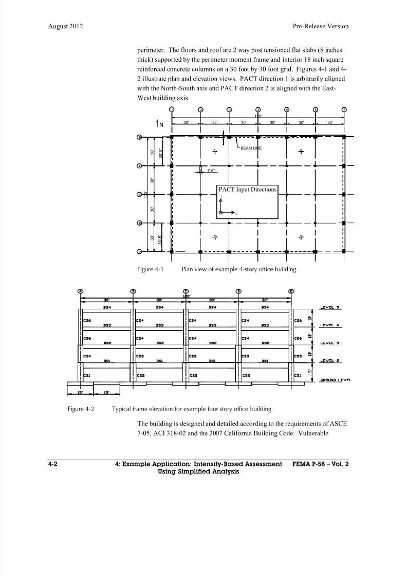
8/12/2019 Seismic Performance Assessment of Buildings
http://slidepdf.com/reader/full/seismic-performance-assessment-of-buildings 140/358

8/12/2019 Seismic Performance Assessment of Buildings
http://slidepdf.com/reader/full/seismic-performance-assessment-of-buildings 141/358
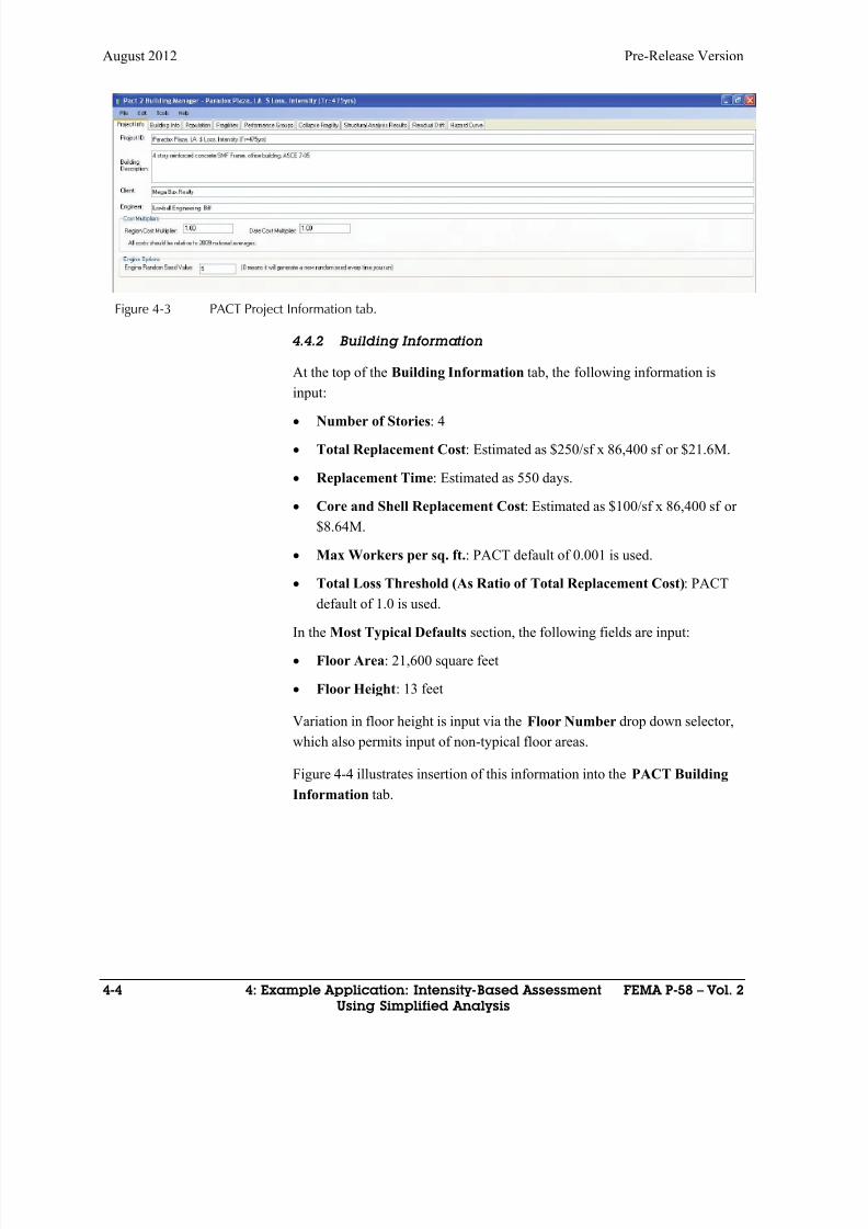
8/12/2019 Seismic Performance Assessment of Buildings
http://slidepdf.com/reader/full/seismic-performance-assessment-of-buildings 142/358
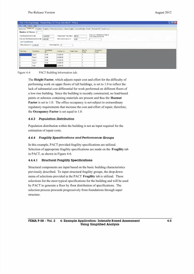
8/12/2019 Seismic Performance Assessment of Buildings
http://slidepdf.com/reader/full/seismic-performance-assessment-of-buildings 143/358
Pre-Release Version August 2012
FEMA P-58 – Vol. 2 4: Example Application: Intensity-Based Assessment 4-5
Using Simplified Analysis
Figure 4-4 PACT Building Information tab.
The Height Factor, which adjusts repair cost and effort for the difficulty of
performing work on upper floors of tall buildings, is set to 1.0 to reflect the
lack of substantial cost differential for work performed on different floors ofa low-rise building. Since the building is recently constructed, no lead-based
paints or asbestos containing materials are present and thus the Hazmat
Factor is set to 1.0. The office occupancy is not subject to extraordinary
regulatory requirements that increase the cost and effort of repair, therefore,
the Occupancy Factor is set equal to 1.0.
4.4.3 Population Distribution
Population distribution within the building is not an input required for the
estimation of repair costs.
4.4.4 Fragility Specifications and Performance Groups
In this example, PACT provided fragility specifications are utilized.
Selection of appropriate fragility specifications are made on the Fragility tab
in PACT, as shown in Figure 4-6.
4.4.4.1 Structural Fragility Specifications
Structural components are input based on the basic building characteristics
previously described. To input structural fragility groups, the drop down
menu of selections provided in the PACT Fragility tab is utilized. These
selections list the most typical specifications for the building and will be used
by PACT to generate a floor by floor distribution of specifications. The
selection process proceeds progressively from foundations through super
structure.
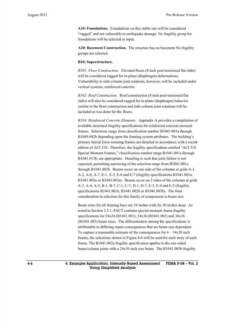
8/12/2019 Seismic Performance Assessment of Buildings
http://slidepdf.com/reader/full/seismic-performance-assessment-of-buildings 144/358
August 2012 Pre-Release Version
4-6 4: Example Application: Intensity-Based Assessment FEMA P-58 – Vol. 2
Using Simplified Analysis
A10: Foundations. Foundations on this stable site will be considered
“rugged” and not vulnerable to earthquake damage. No fragility group for
foundations will be selected or input.
A20: Basement Construction. The structure has no basement No fragility
groups are selected.
B10: Superstructure.
B101: Floor Construction. Elevated floors (8 inch post-tensioned flat slabs)
will be considered rugged for in-plane (diaphragm) deformations.
Vulnerability to slab-column joint rotations, however, will be included under
vertical systems, reinforced concrete.
B102: Roof Construction. Roof construction (8 inch post-tensioned flat
slabs) will also be considered rugged for in-plane (diaphragm) behavior
similar to the floor construction and slab-column joint rotations will beincluded as was done for the floors.
B104: Reinforced Concrete Elements. Appendix A provides a compilation of
available structural fragility specifications for reinforced concrete moment
frames. Selections range from classification number B1041.001a through
B1049.042b depending upon the framing system attributes. The building’s
primary lateral force-resisting frames are detailed in accordance with a recent
edition of ACI 318. Therefore, the fragility specifications entitled “ACI 318
Special Moment Frames,” classification number range B1041.001a through
B1041.013b, are appropriate. Detailing is such that joint failure is not
expected, permitting narrowing of the selection range from B1041.001a
through B1041.003b. Beams occur on one side of the columns at grids A-1,
A-2, A-6, A-7, E-1, E-2, E-6 and E-7 (fragility specifications B1041.001a,
B1041.002a or B1041.003a). Beams occur on 2 sides of the columns at grids
A-3, A-4, A-5, B-1, B-7, C-1, C-7, D-1, D-7, E-3, E-4 and E-5 (fragility
specifications B1041.001b, B1041.002b or B1041.003b). The final
consideration in selection for this family of components is beam size.
Beam sizes for all framing bays are 34 inches wide by 30 inches deep. As
noted in Section 2.5.1, PACT contains special moment frame fragility
specifications for 24x24 (B1041.001), 24x36 (B1041.002) and 36x36
(B1041.003) beam sizes. The differentiation among the specifications is
attributable to differing repair consequences that are beam size dependent.
To capture a reasonable estimate of the consequences for 4 – 34x30 inch
beams, the selections shown in Figure 4-6 will be used for each story of each
frame. The B1041.002a fragility specification applies to the one-sided
beam/column joints with a 24x36 inch size beam. The B1041.003b fragility
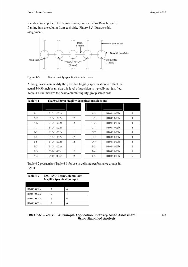
8/12/2019 Seismic Performance Assessment of Buildings
http://slidepdf.com/reader/full/seismic-performance-assessment-of-buildings 145/358
Pre-Release Version August 2012
FEMA P-58 – Vol. 2 4: Example Application: Intensity-Based Assessment 4-7
Using Simplified Analysis
specification applies to the beam/column joints with 36x36 inch beams
framing into the column from each side. Figure 4-5 illustrates this
assignment.
Figure 4-5 Beam fragility specification selections.
Although users can modify the provided fragility specification to reflect the
actual 34x30 inch beam size this level of precision is typically not justified.
Table 4-1 summarizes the beam/column fragility group selections:
Table 4-1 Beam/Column Fragility Specification Selections
JointLocation
Fragility IDInput
Direction Joint
LocationFragility ID
InputDirection
A-1 B1041.002a 1 A-5 B1041.003b 2
A-2 B1041.002a 2 B-1 B1041.003b 1
A-6 B1041.002a 2 B-7 B1041.003b 1
A-7 B1041.002a 1 C-1 B1041.003b 1
E-1 B1041.002a 1 C-7 B1041.003b 1
E-2 B1041.002a 2 D-1 B1041.003b 1
E-6 B1041.002a 2 D-7 B1041.003b 1
E-7 B1041.002a 1 E-3 B1041.003b 2
A-3 B1041.003b 2 E-4 B1041.003b 2
A-4 B1041.003b 2 E-5 B1041.003b 2
Table 4-2 reorganizes Table 4-1 for use in defining performance groups in
PACT:
Table 4-2 PACT SMF Beam/Column JointFragility Specification Input
Fragility ID Direction Number Per Floor
B1041.002a 1 4
B1041.002a 2 4
B1041.003b 1 6
B1041.003b 2 6
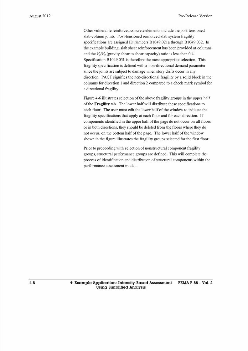
8/12/2019 Seismic Performance Assessment of Buildings
http://slidepdf.com/reader/full/seismic-performance-assessment-of-buildings 146/358
August 2012 Pre-Release Version
4-8 4: Example Application: Intensity-Based Assessment FEMA P-58 – Vol. 2
Using Simplified Analysis
Other vulnerable reinforced concrete elements include the post-tensioned
slab-column joints. Post-tensioned reinforced slab system fragility
specifications are assigned ID numbers B1049.021a through B1049.032. In
the example building, slab shear reinforcement has been provided at columns
and the V g /V 0 (gravity shear to shear capacity) ratio is less than 0.4.
Specification B1049.031 is therefore the most appropriate selection. This
fragility specification is defined with a non-directional demand parameter
since the joints are subject to damage when story drifts occur in any
direction. PACT signifies the non-directional fragility by a solid block in the
columns for direction 1 and direction 2 compared to a check mark symbol for
a directional fragility.
Figure 4-6 illustrates selection of the above fragility groups in the upper half
of the Fragility tab. The lower half will distribute these specifications to
each floor. The user must edit the lower half of the window to indicate the
fragility specifications that apply at each floor and for each direction. Ifcomponents identified in the upper half of the page do not occur on all floors
or in both directions, they should be deleted from the floors where they do
not occur, on the bottom half of the page. The lower half of the window
shown in the figure illustrates the fragility groups selected for the first floor.
Prior to proceeding with selection of nonstructural component fragility
groups, structural performance groups are defined. This will complete the
process of identification and distribution of structural components within the
performance assessment model.
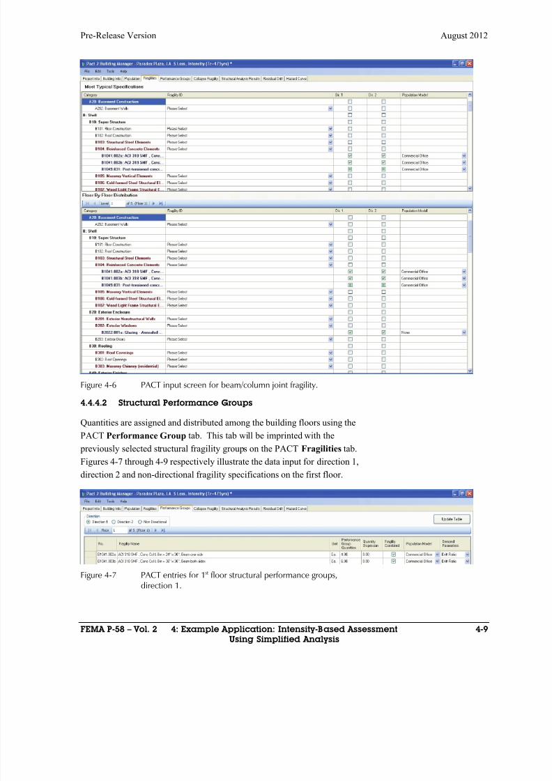
8/12/2019 Seismic Performance Assessment of Buildings
http://slidepdf.com/reader/full/seismic-performance-assessment-of-buildings 147/358
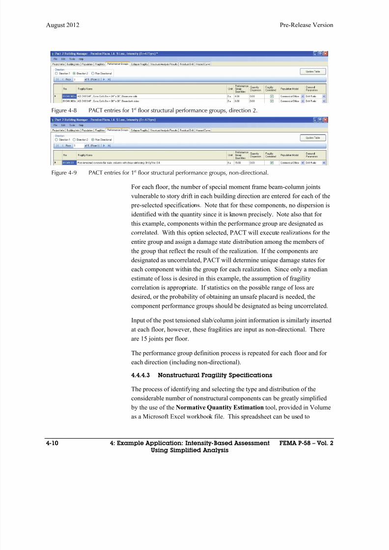
8/12/2019 Seismic Performance Assessment of Buildings
http://slidepdf.com/reader/full/seismic-performance-assessment-of-buildings 148/358
August 2012 Pre-Release Version
4-10 4: Example Application: Intensity-Based Assessment FEMA P-58 – Vol. 2
Using Simplified Analysis
Figure 4-8 PACT entries for 1st floor structural performance groups, direction 2.
Figure 4-9 PACT entries for 1st floor structural performance groups, non-directional.
For each floor, the number of special moment frame beam-column joints
vulnerable to story drift in each building direction are entered for each of the
pre-selected specifications. Note that for these components, no dispersion is
identified with the quantity since it is known precisely. Note also that for
this example, components within the performance group are designated as
correlated. With this option selected, PACT will execute realizations for the
entire group and assign a damage state distribution among the members of
the group that reflect the result of the realization. If the components are
designated as uncorrelated, PACT will determine unique damage states for
each component within the group for each realization. Since only a medianestimate of loss is desired in this example, the assumption of fragility
correlation is appropriate. If statistics on the possible range of loss are
desired, or the probability of obtaining an unsafe placard is needed, the
component performance groups should be designated as being uncorrelated.
Input of the post tensioned slab/column joint information is similarly inserted
at each floor, however, these fragilities are input as non-directional. There
are 15 joints per floor.
The performance group definition process is repeated for each floor and for
each direction (including non-directional).
4.4.4.3 Nonstructural Fragility Specifications
The process of identifying and selecting the type and distribution of the
considerable number of nonstructural components can be greatly simplified
by the use of the Normative Quantity Estimation tool, provided in Volume
as a Microsoft Excel workbook file. This spreadsheet can be used to
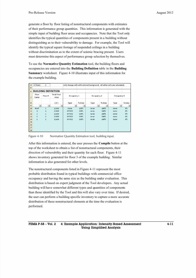
8/12/2019 Seismic Performance Assessment of Buildings
http://slidepdf.com/reader/full/seismic-performance-assessment-of-buildings 149/358
Pre-Release Version August 2012
FEMA P-58 – Vol. 2 4: Example Application: Intensity-Based Assessment 4-11
Using Simplified Analysis
generate a floor by floor listing of nonstructural components with estimates
of their performance group quantities. This information is generated with the
simple input of building floor areas and occupancies. Note that the Tool only
identifies the typical quantities of components present in a building without
distinguishing as to their vulnerability to damage. For example, the Tool will
identify the typical square footage of suspended ceilings in a building
without discrimination as to the extent of seismic bracing present. Users
must determine this aspect of performance group selection by themselves.
To use the Normative Quantity Estimation tool, the building floors and
occupancies are entered into the Building Definition table in the Building
Summary worksheet. Figure 4-10 illustrates input of this information for
the example building.
Figure 4-10 Normative Quantity Estimation tool, building input.
After this information is entered, the user presses the Compile button at the
top of the worksheet to obtain a list of nonstructural components, their
direction of vulnerability and their quantity for each floor. Figure 4-11
shows inventory generated for floor 3 of the example building. Similar
information is also generated for other levels.
The nonstructural components listed in Figure 4-11 represent the most
probable distribution found in typical buildings with commercial office
occupancy and having the same size as the building under evaluation. This
distribution is based on expert judgment of the Tool developers. Any actual
building will have somewhat different types and quantities of components
than those identified by the Tool and this will also vary over time. If desired,
the user can perform a building specific inventory to capture a more accurate
distribution of these nonstructural elements at the time the evaluation is
performed.
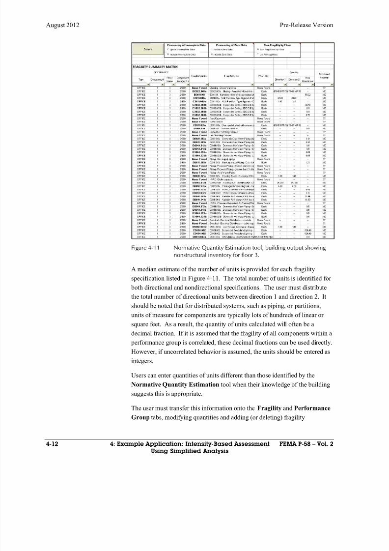
8/12/2019 Seismic Performance Assessment of Buildings
http://slidepdf.com/reader/full/seismic-performance-assessment-of-buildings 150/358
August 2012 Pre-Release Version
4-12 4: Example Application: Intensity-Based Assessment FEMA P-58 – Vol. 2
Using Simplified Analysis
Figure 4-11 Normative Quantity Estimation tool, building output showingnonstructural inventory for floor 3.
A median estimate of the number of units is provided for each fragilityspecification listed in Figure 4-11. The total number of units is identified for
both directional and nondirectional specifications. The user must distribute
the total number of directional units between direction 1 and direction 2. It
should be noted that for distributed systems, such as piping, or partitions,
units of measure for components are typically lots of hundreds of linear or
square feet. As a result, the quantity of units calculated will often be a
decimal fraction. If it is assumed that the fragility of all components within a
performance group is correlated, these decimal fractions can be used directly.
However, if uncorrelated behavior is assumed, the units should be entered as
integers.
Users can enter quantities of units different than those identified by the
Normative Quantity Estimation tool when their knowledge of the building
suggests this is appropriate.
The user must transfer this information onto the Fragility and Performance
Group tabs, modifying quantities and adding (or deleting) fragility
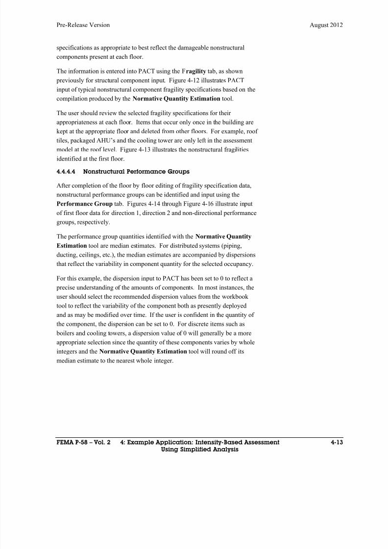
8/12/2019 Seismic Performance Assessment of Buildings
http://slidepdf.com/reader/full/seismic-performance-assessment-of-buildings 151/358
Pre-Release Version August 2012
FEMA P-58 – Vol. 2 4: Example Application: Intensity-Based Assessment 4-13
Using Simplified Analysis
specifications as appropriate to best reflect the damageable nonstructural
components present at each floor.
The information is entered into PACT using the Fragility tab, as shown
previously for structural component input. Figure 4-12 illustrates PACT
input of typical nonstructural component fragility specifications based on thecompilation produced by the Normative Quantity Estimation tool.
The user should review the selected fragility specifications for their
appropriateness at each floor. Items that occur only once in the building are
kept at the appropriate floor and deleted from other floors. For example, roof
tiles, packaged AHU’s and the cooling tower are only left in the assessment
model at the roof level. Figure 4-13 illustrates the nonstructural fragilities
identified at the first floor.
4.4.4.4 Nonstructural Performance Groups
After completion of the floor by floor editing of fragility specification data,
nonstructural performance groups can be identified and input using the
Performance Group tab. Figures 4-14 through Figure 4-16 illustrate input
of first floor data for direction 1, direction 2 and non-directional performance
groups, respectively.
The performance group quantities identified with the Normative Quantity
Estimation tool are median estimates. For distributed systems (piping,
ducting, ceilings, etc.), the median estimates are accompanied by dispersions
that reflect the variability in component quantity for the selected occupancy.
For this example, the dispersion input to PACT has been set to 0 to reflect a
precise understanding of the amounts of components. In most instances, the
user should select the recommended dispersion values from the workbook
tool to reflect the variability of the component both as presently deployed
and as may be modified over time. If the user is confident in the quantity of
the component, the dispersion can be set to 0. For discrete items such as
boilers and cooling towers, a dispersion value of 0 will generally be a more
appropriate selection since the quantity of these components varies by whole
integers and the Normative Quantity Estimation tool will round off its
median estimate to the nearest whole integer.
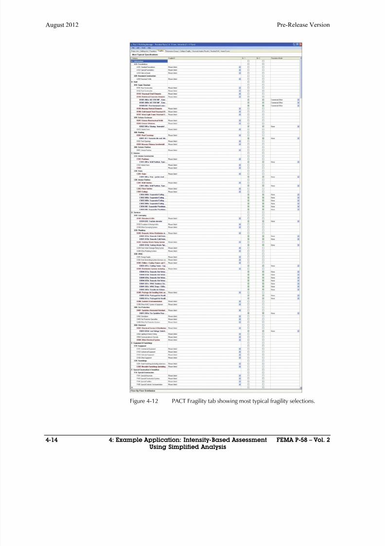
8/12/2019 Seismic Performance Assessment of Buildings
http://slidepdf.com/reader/full/seismic-performance-assessment-of-buildings 152/358
August 2012 Pre-Release Version
4-14 4: Example Application: Intensity-Based Assessment FEMA P-58 – Vol. 2
Using Simplified Analysis
Figure 4-12 PACT Fragility tab showing most typical fragility selections.
8/12/2019 Seismic Performance Assessment of Buildings
http://slidepdf.com/reader/full/seismic-performance-assessment-of-buildings 153/358

8/12/2019 Seismic Performance Assessment of Buildings
http://slidepdf.com/reader/full/seismic-performance-assessment-of-buildings 154/358
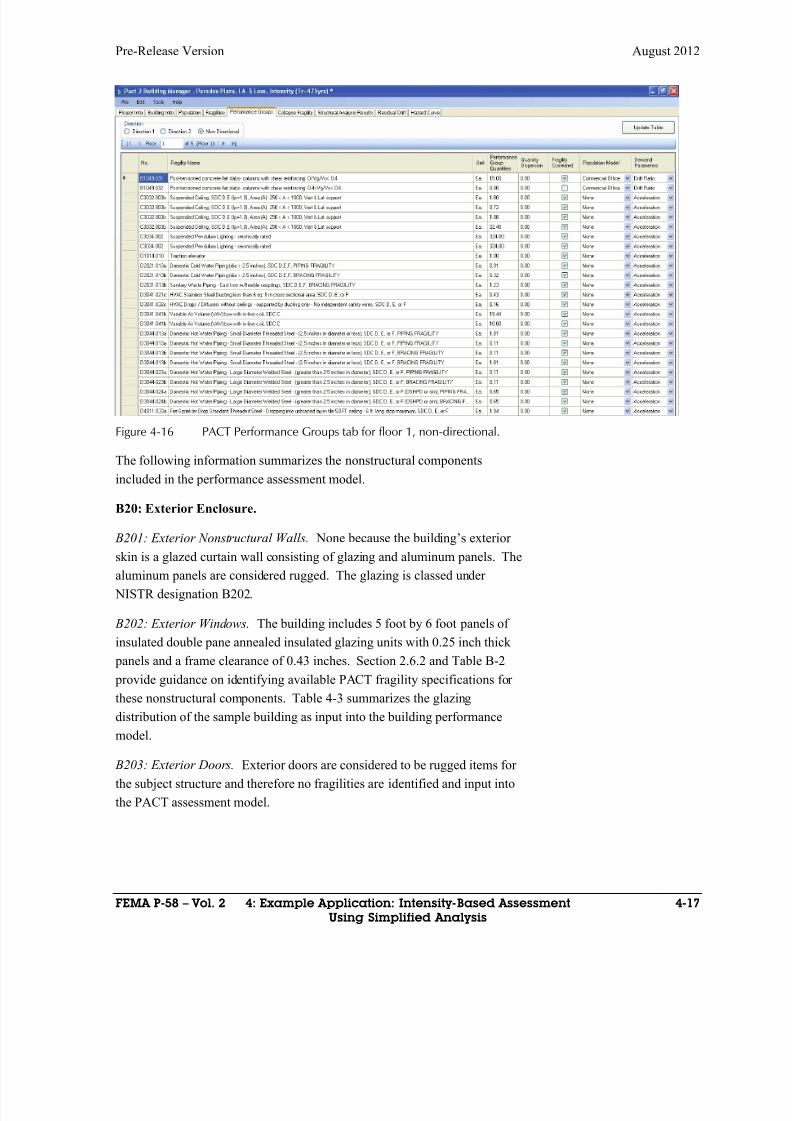
8/12/2019 Seismic Performance Assessment of Buildings
http://slidepdf.com/reader/full/seismic-performance-assessment-of-buildings 155/358
Pre-Release Version August 2012
FEMA P-58 – Vol. 2 4: Example Application: Intensity-Based Assessment 4-17
Using Simplified Analysis
Figure 4-16 PACT Performance Groups tab for floor 1, non-directional.
The following information summarizes the nonstructural components
included in the performance assessment model.
B20: Exterior Enclosure.
B201: Exterior Nonstructural Walls. None because the building’s exterior
skin is a glazed curtain wall consisting of glazing and aluminum panels. The
aluminum panels are considered rugged. The glazing is classed under
NISTR designation B202.
B202: Exterior Windows. The building includes 5 foot by 6 foot panels of
insulated double pane annealed insulated glazing units with 0.25 inch thick
panels and a frame clearance of 0.43 inches. Section 2.6.2 and Table B-2
provide guidance on identifying available PACT fragility specifications for
these nonstructural components. Table 4-3 summarizes the glazing
distribution of the sample building as input into the building performance
model.
B203: Exterior Doors. Exterior doors are considered to be rugged items for
the subject structure and therefore no fragilities are identified and input into
the PACT assessment model.
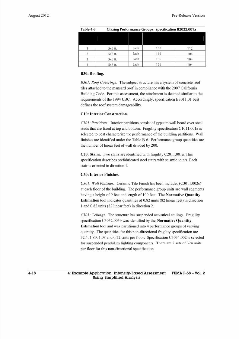
8/12/2019 Seismic Performance Assessment of Buildings
http://slidepdf.com/reader/full/seismic-performance-assessment-of-buildings 156/358
August 2012 Pre-Release Version
4-18 4: Example Application: Intensity-Based Assessment FEMA P-58 – Vol. 2
Using Simplified Analysis
Table 4-3 Glazing Performance Groups: Specification B2022.001a
Floor Panel Dimensions Units Total Direction 1 Total Direction 2
1 5x6 ft. Each 168 112
2 5x6 ft. Each 156 1043 5x6 ft. Each 156 104
4 5x6 ft. Each 156 104
B30: Roofing.
B301: Roof Coverings. The subject structure has a system of concrete roof
tiles attached to the mansard roof in compliance with the 2007 California
Building Code. For this assessment, the attachment is deemed similar to the
requirements of the 1994 UBC. Accordingly, specification B3011.01 best
defines the roof system damageability.
C10: Interior Construction.
C101: Partitions. Interior partitions consist of gypsum wall board over steel
studs that are fixed at top and bottom. Fragility specification C1011.001a is
selected to best characterize the performance of the building partitions. Wall
finishes are identified under the Table B-6. Performance group quantities are
the number of linear feet of wall divided by 200.
C20: Stairs. Two stairs are identified with fragility C2011.001a. This
specification describes prefabricated steel stairs with seismic joints. Each
stair is oriented in direction 1.
C30: Interior Finishes.
C301: Wall Finishes. Ceramic Tile Finish has been included (C3011.002c)
at each floor of the building. The performance group units are wall segments
having a height of 9 feet and length of 100 feet. The Normative Quantity
Estimation tool indicates quantities of 0.82 units (82 linear feet) in direction
1 and 0.82 units (82 linear feet) in direction 2.
C303: Ceilings. The structure has suspended acoustical ceilings. Fragility
specification C3032.003b was identified by the Normative QuantityEstimation tool and was partitioned into 4 performance groups of varying
quantity. The quantities for this non-directional fragility specification are
32.4, 1.80, 1.08 and 0.72 units per floor. Specification C3034.002 is selected
for suspended pendulum lighting components. There are 2 sets of 324 units
per floor for this non-directional specification.
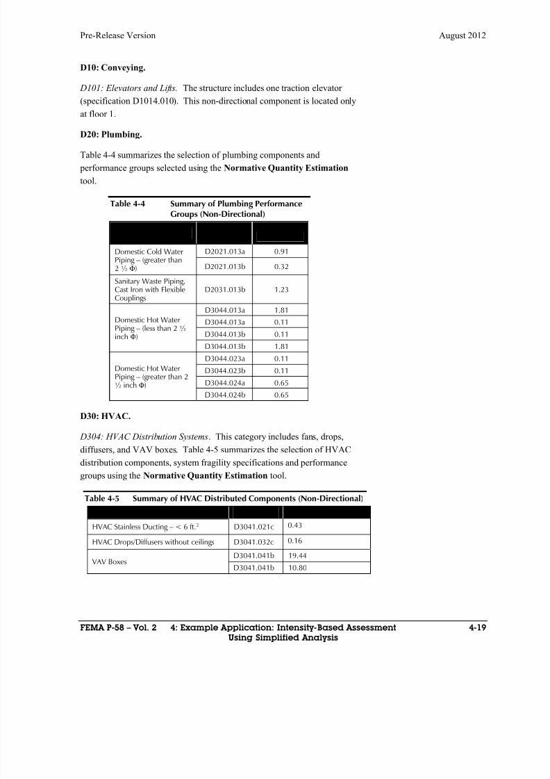
8/12/2019 Seismic Performance Assessment of Buildings
http://slidepdf.com/reader/full/seismic-performance-assessment-of-buildings 157/358
Pre-Release Version August 2012
FEMA P-58 – Vol. 2 4: Example Application: Intensity-Based Assessment 4-19
Using Simplified Analysis
D10: Conveying.
D101: Elevators and Lifts. The structure includes one traction elevator
(specification D1014.010). This non-directional component is located only
at floor 1.
D20: Plumbing.
Table 4-4 summarizes the selection of plumbing components and
performance groups selected using the Normative Quantity Estimation
tool.
Table 4-4 Summary of Plumbing PerformanceGroups (Non-Directional)
General Description Fragility IDQuantity Per
Floor
Domestic Cold WaterPiping – (greater than2 ½ Φ)
D2021.013a 0.91D2021.013b 0.32
Sanitary Waste Piping,Cast Iron with FlexibleCouplings
D2031.013b 1.23
Domestic Hot WaterPiping – (less than 2 ½inch Φ)
D3044.013a 1.81
D3044.013a 0.11
D3044.013b 0.11
D3044.013b 1.81
Domestic Hot WaterPiping – (greater than 2
½ inch Φ)
D3044.023a 0.11
D3044.023b 0.11
D3044.024a 0.65D3044.024b 0.65
D30: HVAC.
D304: HVAC Distribution Systems. This category includes fans, drops,
diffusers, and VAV boxes. Table 4-5 summarizes the selection of HVAC
distribution components, system fragility specifications and performance
groups using the Normative Quantity Estimation tool.
Table 4-5 Summary of HVAC Distributed Components (Non-Directional)
General Description Fragility ID Quantity Per Floor
HVAC Stainless Ducting – < 6 ft.2 D3041.021c 0.43
HVAC Drops/Diffusers without ceilings D3041.032c 0.16
VAV BoxesD3041.041b 19.44
D3041.041b 10.80
8/12/2019 Seismic Performance Assessment of Buildings
http://slidepdf.com/reader/full/seismic-performance-assessment-of-buildings 158/358
August 2012 Pre-Release Version
4-20 4: Example Application: Intensity-Based Assessment FEMA P-58 – Vol. 2
Using Simplified Analysis
D306: Packaged Air Handling Units. D3052.013b and D3052.011a were
placed at the first floor and oriented in direction 1. The Normative
Quantity Estimation tool recommends 243 units of D3052.013b and 4 units
of D3052.011a.
D40: Fire Protection.
D401: Fire Sprinkler . Fragility specification D4011.033a was selected for
suppression sprinklers. Sprinkler drop fragility specifications are divided
into 3 categories that reflect soft-lay-in tile ceilings, hard-lay-in tile ceilings,
and no ceilings. In this example, a soft-lay-in tile ceiling is assumed. It is
further assumed that since the building is of recent construction, the ceiling
bracing conforms to Seismic Design Category D, E, or F to appropriately
reflect the seismic hazard of the Los Angeles site. The fragility specification
for D4011.033a identifies the units of measure for fire sprinklers as 1,000
linear feet run of distribution piping, including drops and heads. TheNormative Quantity Estimation tool identifies 1.94 units (1,940 linear feet
of sprinkler piping) at each floor.
D50: Electrical. Low Voltage Switchgear (D5012.023d) is provided in each
direction at each floor level.
Equipment and furnishings and fragilities for special construction were not
considered.
4.4.5 Collapse Fragility and Collapse Modes
4.4.5.1 Collapse Fragility
Volume 1, Chapter 6 discusses three approaches for development of collapse
fragility. This example demonstrates the use of the nonlinear static approach
as summarized in Section 2.6.2.
Step 1. Construct a mathematical model of the building for nonlinear static
analysis in each building direction. For the example structure, each building
direction has identical strength and stiffness characteristics so only one
analysis is needed.
Step 2. Nonlinear static analysis was performed to identify the sequence ofcomponent yielding to a deformation at which collapse is judged to occur.
Step 3. Figure 4-17 illustrates the results of the pushover analysis for both
building direction 1 and direction 2, which are identical. Collapse is judged
to occur at a roof drift of 2.7 feet, which corresponds to a roof drift ratio of
5%.
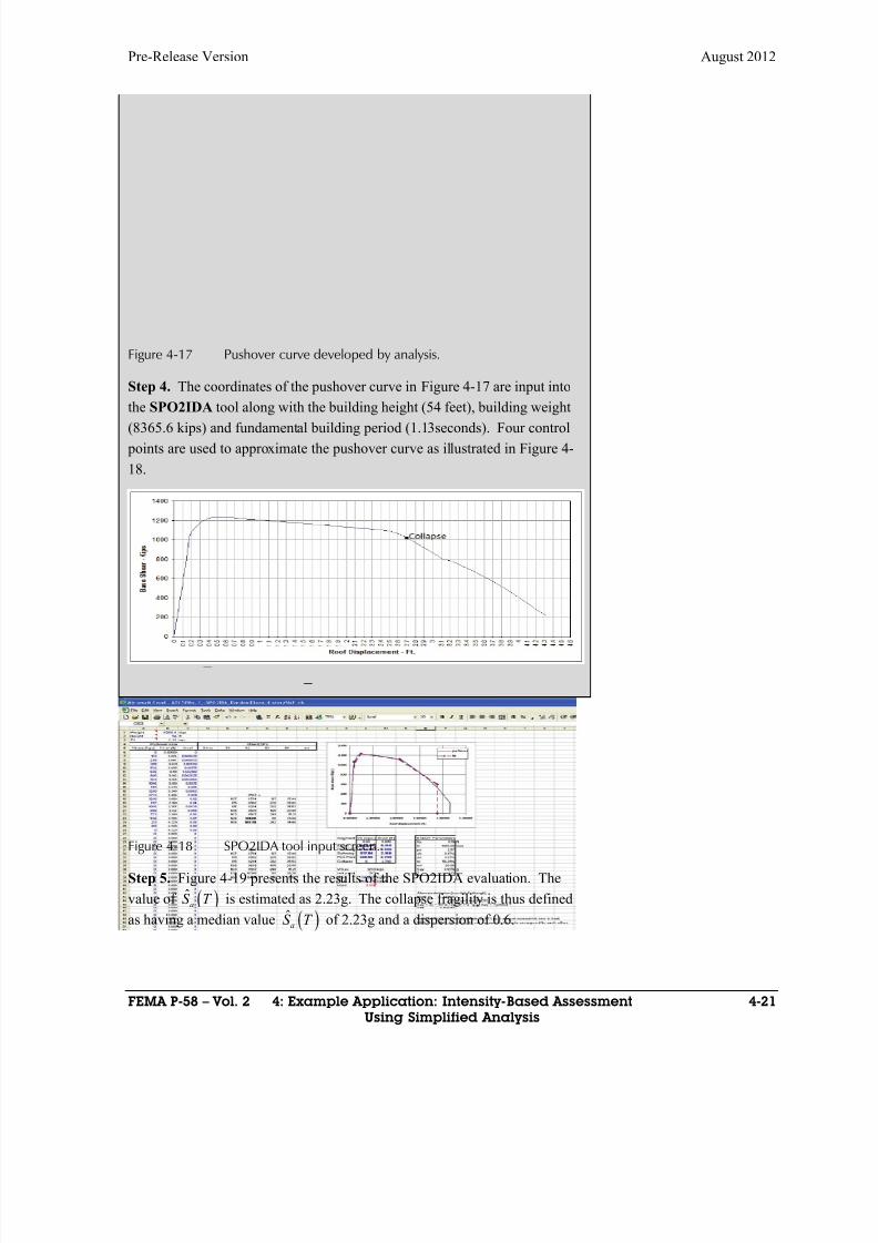
8/12/2019 Seismic Performance Assessment of Buildings
http://slidepdf.com/reader/full/seismic-performance-assessment-of-buildings 159/358
Pre-Release Version August 2012
FEMA P-58 – Vol. 2 4: Example Application: Intensity-Based Assessment 4-21
Using Simplified Analysis
Figure 4-17 Pushover curve developed by analysis.
Step 4. The coordinates of the pushover curve in Figure 4-17 are input into
the SPO2IDA tool along with the building height (54 feet), building weight(8365.6 kips) and fundamental building period (1.13seconds). Four control
points are used to approximate the pushover curve as illustrated in Figure 4-
18.
Figure 4-18 SPO2IDA tool input screen.
Step 5. Figure 4-19 presents the results of the SPO2IDA evaluation. The
value of ˆaS T is estimated as 2.23g. The collapse fragility is thus defined
as having a median value ˆaS T of 2.23g and a dispersion of 0.6.
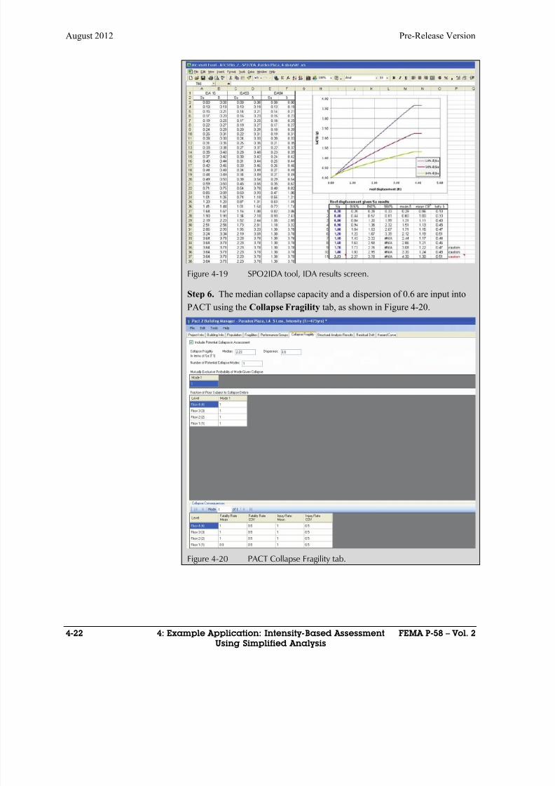
8/12/2019 Seismic Performance Assessment of Buildings
http://slidepdf.com/reader/full/seismic-performance-assessment-of-buildings 160/358
August 2012 Pre-Release Version
4-22 4: Example Application: Intensity-Based Assessment FEMA P-58 – Vol. 2
Using Simplified Analysis
Figure 4-19 SPO2IDA tool, IDA results screen.
Step 6. The median collapse capacity and a dispersion of 0.6 are input into
PACT using the Collapse Fragility tab, as shown in Figure 4-20.
Figure 4-20 PACT Collapse Fragility tab.
8/12/2019 Seismic Performance Assessment of Buildings
http://slidepdf.com/reader/full/seismic-performance-assessment-of-buildings 161/358
Pre-Release Version August 2012
FEMA P-58 – Vol. 2 4: Example Application: Intensity-Based Assessment 4-23
Using Simplified Analysis
4.4.5.2 Collapse Modes
PACT collapse mode input includes the number of independent collapse
modes that can occur and the probability of each. This is difficult to predict
analytically. To determine these data, the user must use judgment based on
upon building type, structural system, past experience, and analyticalinferences. When using the simplified analysis approach, limited analytical
information regarding potential collapse modes is available. For this
example, only a single mode of collapse is considered. In the next chapter, a
more complex pattern of potential collapse modes is identified. The
additional information gained from numerous response history analyses can
provide additional insight into potential collapse modes.
PACT input also includes the fraction of each floor subject to collapse-
associated debris and the resulting fatality and injury rates. These must also
be determined judgmentally. Figure 4-20 shows the input values for thisexample.
4.4.6 Residual Drift Fragility
The PACT default residual drift fragility is modified for this assessment.
The median residual drift at which damage will be deemed irreparable is
increased to 0.0125, as shown in Figure 4-21. The estimated median
building residual drift demand and dispersion are input to this tab after the
analysis is completed.
4.5 Select Analysis Method and Construct Building
Analytical Model
The simplified analysis method is used to generate median estimates of peak
transient drift, peak floor accelerations and residual drifts. Associated
dispersions are generated using the simplified analysis method. Peak total
floor velocities are not generated since none of the vulnerable building
components use this demand parameter. A linear building model is
constructed using the modeling criteria of ASCE/SEI 41-06, Linear Static
Procedure.

8/12/2019 Seismic Performance Assessment of Buildings
http://slidepdf.com/reader/full/seismic-performance-assessment-of-buildings 162/358
August 2012 Pre-Release Version
4-24 4: Example Application: Intensity-Based Assessment FEMA P-58 – Vol. 2
Using Simplified Analysis
Figure 4-21 PACT Residual Drift fragility.
4.6 Define Earthquake Hazards
The target intensity is given as earthquake ground shaking with an average
return period of 475 years. Using the simplified analysis method to predict
peak transient drifts, peak floor accelerations and residual drifts, thefollowing ground motion parameters will be required: S a(T 1
X ), S a(T 1Y ),
S a(T =0).
From analysis the building’s periods are determined as T 1 X = T 1
Y = 1.13
seconds.
The ground motion parameters are generated using the ground motion
calculator on the USGS website, available as a downloadable Java
application. This application permits calculation of seismic hazard curves for
sites conforming to ASCE/SEI 7-10 Site Class B at the following discrete
building periods: 0, 0.1, 0.2, 0.3, 0.5, 1.0 and 2.0 seconds. For intermediate
periods, the value of S a can be determined by constructing the spectrum using
the above values and graphically determining the value of S a(T ). For
structures with periods in the range of 0.7 seconds < T <2.0 seconds, it is
typically sufficiently accurate to obtain S a(T ) from the formula:
1.0a
a
S S T
T

8/12/2019 Seismic Performance Assessment of Buildings
http://slidepdf.com/reader/full/seismic-performance-assessment-of-buildings 163/358
Pre-Release Version August 2012
FEMA P-58 – Vol. 2 4: Example Application: Intensity-Based Assessment 4-25
Using Simplified Analysis
Figure 4-22 illustrates the input of the building site’s coordinates and the
tabular output for the spectral acceleration values at a period of 1.0 second
and their mean annual frequency of exceedance (MAFE) at the building site.
Figure 4-22 USGS seismic hazard output.
Table 4-6 shows the spectral acceleration values and mean annual frequency
of exceedance obtained from the ground motion calculator, the value of F v
obtained from ASCE/SEI 7-10 at each MAFE, and the value of S a1.13
derived using the above formula with sT 13.1 . Figure 4-23 is a plot of
these data evaluated at the building average period and presented in log-
linear form.
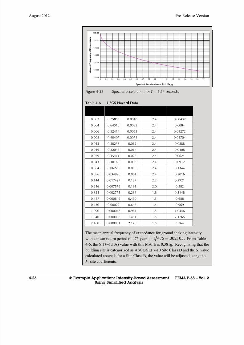
8/12/2019 Seismic Performance Assessment of Buildings
http://slidepdf.com/reader/full/seismic-performance-assessment-of-buildings 164/358
August 2012 Pre-Release Version
4-26 4: Example Application: Intensity-Based Assessment FEMA P-58 – Vol. 2
Using Simplified Analysis
Figure 4-23 Spectral acceleration for T = 1.13 seconds.
Table 4-6 USGS Hazard Data
Sa(T=1.00s)
Site Class B MAFE
Sa(T=1.13s)
Site Class B F v Sa(T = 1.13s)
0.002 0.75855 0.0018 2.4 0.00432
0.004 0.64518 0.0035 2.4 0.0084
0.006 0.52414 0.0053 2.4 0.01272
0.008 0.40407 0.0071 2.4 0.01704
0.013 0.30233 0.012 2.4 0.0288
0.019 0.22048 0.017 2.4 0.0408
0.029 0.15411 0.026 2.4 0.0624
0.043 0.10169 0.038 2.4 0.0912
0.064 0.06226 0.056 2.4 0.13440.096 0.034926 0.084 2.4 0.2016
0.144 0.017497 0.127 2.2 0.2921
0.216 0.007576 0.191 2.0 0.382
0.324 0.002775 0.286 1.8 0.5148
0.487 0.000849 0.430 1.5 0.688
0.730 0.00022 0.646 1.5 0.969
1.090 0.000048 0.964 1.5 1.0446
1.640 0.000008 1.451 1.5 2.1765
2.460 0.000001 2.176 1.5 3.264
The mean annual frequency of exceedance for ground shaking intensity
with a mean return period of 475 years is 002105.4751 . From Table
4-6, the S a (T =1.13s) value with this MAFE is 0.381g. Recognizing that the
building site is categorized as ASCE/SEI 7-10 Site Class D and the S a value
calculated above is for a Site Class B, the value will be adjusted using the
F v site coefficients.
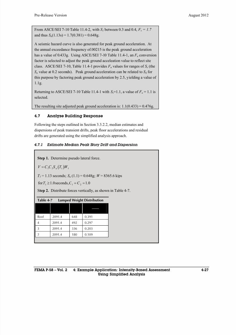
8/12/2019 Seismic Performance Assessment of Buildings
http://slidepdf.com/reader/full/seismic-performance-assessment-of-buildings 165/358
Pre-Release Version August 2012
FEMA P-58 – Vol. 2 4: Example Application: Intensity-Based Assessment 4-27
Using Simplified Analysis
From ASCE/SEI 7-10 Table 11.4-2, with S 1 between 0.3 and 0.4, F v = 1.7
and thus S a(1.13s) = 1.7(0.381) = 0.648g.
A seismic hazard curve is also generated for peak ground acceleration. At
the annual exceedance frequency of.00215 is the peak ground acceleration
has a value of 0.433g. Using ASCE/SEI 7-10 Table 11.4-1, an F a conversionfactor is selected to adjust the peak ground acceleation value to reflect site
class. ASCE/SEI 7-10, Table 11.4-1 provides F a values for ranges of S s (the
S a value at 0.2 seconds). Peak ground acceleration can be related to S S for
this purpose by factoring peak ground acceleration by 2.5, yielding a value of
1.1g.
Returning to ASCE/SEI 7-10 Table 11.4-1 with S s=1.1, a value of F a = 1.1 is
selected.
The resulting site adjusted peak ground acceleration is: 1.1(0.433) = 0.476g.
4.7 Analyze Building Response
Following the steps outlined in Section 3.3.2.2, median estimates and
dispersions of peak transient drifts, peak floor accelerations and residual
drifts are generated using the simplified analysis approach.
4.7.1 Estimate Median Peak Story Drift and Dispersion
Step 1. Determine pseudo lateral force.
1 2 1 1aV C C S T W
T 1 = 1.13 seconds; S a (1.1) = 0.648g; W = 8365.6 kips
1 1 2for 1.0 seconds , 1.0T C C
Step 2. Distribute forces vertically, as shown in Table 4-7.
Table 4-7 Lumped Weight Distribution
Floor W h (in.)
∑
Roof 2091.4 648 0.391
4 2091.4 492 0.297
3 2091.4 336 0.203
2 2091.4 180 0.109
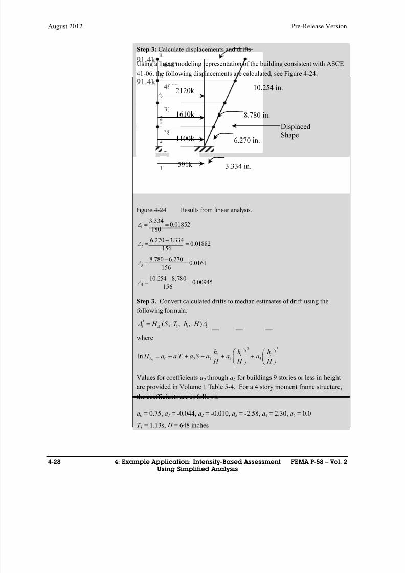
8/12/2019 Seismic Performance Assessment of Buildings
http://slidepdf.com/reader/full/seismic-performance-assessment-of-buildings 166/358
August 2012 Pre-Release Version
4-28 4: Example Application: Intensity-Based Assessment FEMA P-58 – Vol. 2
Using Simplified Analysis
Step 3: Calculate displacements and drifts.
Using a linear modeling representation of the building consistent with ASCE
41-06, the following displacements are calculated, see Figure 4-24:
10.254 in.
8.780 in.
6.270 in.
3.334 in.
2120k
1610k
1100k
591k
4
3
2
1
Displaced
Shape
Figure 4-24 Results from linear analysis.
1
3.3340.01852
180
2
6.270 3.3340.01882
156
3
8.780 6.2700.0161
156
4
10.254 8.7800.00945156
Step 3. Convert calculated drifts to median estimates of drift using the
following formula:
*
1( , , , )ii i i H S T h H
where
2 3
0 1 1 2 3 4 5lni
i i ih h h
H a a T a S a a a H H H
Values for coefficients a0 through a5 for buildings 9 stories or less in height
are provided in Volume 1 Table 5-4. For a 4 story moment frame structure,
the coefficients are as follows:
a0 = 0.75, a1 = -0.044, a2 = -0.010, a3 = -2.58, a4 = 2.30, a5 = 0.0
T 1 = 1.13s, H = 648 inches
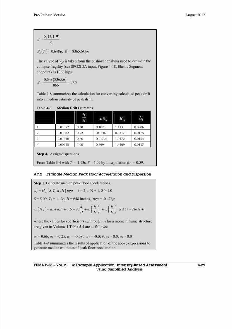
8/12/2019 Seismic Performance Assessment of Buildings
http://slidepdf.com/reader/full/seismic-performance-assessment-of-buildings 167/358
Pre-Release Version August 2012
FEMA P-58 – Vol. 2 4: Example Application: Intensity-Based Assessment 4-29
Using Simplified Analysis
4.7.2 Estimate Median Peak Floor Acceleration and Dispersion
Step 1. Generate median peak floor accelerations.
*
1, , ,ii a i
a H S T h H pga i = 2 to N + 1, S ≥ 1.0
S = 5.09, T 1 = 1.13s, H = 648 inches, pga = 0.476 g
2 3
0 1 1 2 3 4 5 1 2 1i i iai
h h hln H a a T a S a a a S i to N
H H H
where the values for coefficients a0 through a5 for a moment frame structure
are given in Volume 1 Table 5-4 are as follows:
a0 = 0.66, a1 = -0.25, a2 = -0.080, a3 = -0.039, a4 = 0.0, a5 = 0.0
Table 4-9 summarizes the results of application of the above expressions togenerate median estimates of peak floor acceleration.
1
1a
y
S T W S
V
1
0.648 , 8365.6a
S T g W kips
The valyue of is taken from the pushover analysis used to estimate the
collapse fragility (see SPO2IDA input, Figure 4-18, Elastic Segment
endpoint) as 1066 kips.
0.648 8365.65.09
1066S
Table 4-8 summarizes the calculation for converting calculated peak drift
into a median estimate of peak drift.
Table 4-8 Median Drift Estimates
Story Δi
1 0.01852 0.28 0.1073 1.113 0.0206
2 0.01882 0.52 -0.0707 0.9317 0.0175
3 0.01610 0.76 0.01708 1.0172 0.0164
4 0.00945 1.00 0.3694 1.4469 0.0137
Step 4. Assign dispersions.
From Table 3-4 with T 1 = 1.13s, S = 5.09 by interpolation β SD = 0.59.

8/12/2019 Seismic Performance Assessment of Buildings
http://slidepdf.com/reader/full/seismic-performance-assessment-of-buildings 168/358
August 2012 Pre-Release Version
4-30 4: Example Application: Intensity-Based Assessment FEMA P-58 – Vol. 2
Using Simplified Analysis
4.7.3 Estimate Median Residual Story Drift and Dispersion
Step 1. Generate median residual drift.
Residual drift is determined by the difference between peak transient drift
and yield drift. The peak transient drifts were estimated in Section 4.7.1.
The yield drift is from the pushover analysis used to generate the story shear
at yield. From Figure 4-18, the roof displacement at yield is 0.189 feet or
2.268 inches. The yield drift is
2.2680.00350
648 y
The maximum transient drift for the building occurs at the first story
(0.0206). The maximum residual drift is therefore
* max 0.0206 3.1 0.0035 0.00975r
Note that for *
i substantially greater than 4 , y the linear method may not
be reliable for estimating seismic demands. In this example,
*
1 0.02065.9
0.0035 y
This significantly exceeds the recommended limitation on the degree ofinelastic behavior for which the linear approach is appropriate. At higher
levels of nonlinearity, the effects of component degradation and P- Δ may
result in an underestimation of median demand. The median estimate of
residual drift obtained from the simplified analysis method is assigned a
dispersion of 0.8.
Table 4-9 Median Floor Acceleration Estimates
Floor pga
1 0.476 - - - 0.4762 0.476 0.28 -0.04062 0.9602 0.457
3 0.476 0.52 -0.05000 0.9512 0.453
4 0.476 0.76 -0.05934 0.9424 0.449
5 0.476 1.00 -0.06870 0.9336 0.444
Step 2. Assign dispersions.
From Table 3-5 with T 1 = 1.13s and S = 5.09 by interpolation β FA = 0.48.
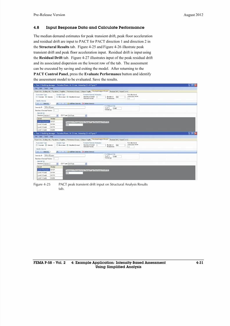
8/12/2019 Seismic Performance Assessment of Buildings
http://slidepdf.com/reader/full/seismic-performance-assessment-of-buildings 169/358
Pre-Release Version August 2012
FEMA P-58 – Vol. 2 4: Example Application: Intensity-Based Assessment 4-31
Using Simplified Analysis
4.8 Input Response Data and Calculate Performance
The median demand estimates for peak transient drift, peak floor acceleration
and residual drift are input to PACT for PACT direction 1 and direction 2 in
the Structural Results tab. Figure 4-25 and Figure 4-26 illustrate peak
transient drift and peak floor acceleration input. Residual drift is input usingthe Residual Drift tab. Figure 4-27 illustrates input of the peak residual drift
and its associated dispersion on the lowest row of the tab. The assessment
can be executed by saving and exiting the model. After returning to the
PACT Control Panel, press the Evaluate Performance button and identify
the assessment model to be evaluated. Save the results.
Figure 4-25 PACT peak transient drift input on Structural Analysis Resultstab.
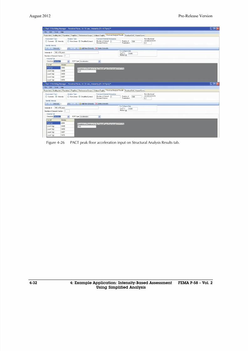
8/12/2019 Seismic Performance Assessment of Buildings
http://slidepdf.com/reader/full/seismic-performance-assessment-of-buildings 170/358
August 2012 Pre-Release Version
4-32 4: Example Application: Intensity-Based Assessment FEMA P-58 – Vol. 2
Using Simplified Analysis
Figure 4-26 PACT peak floor acceleration input on Structural Analysis Results tab.
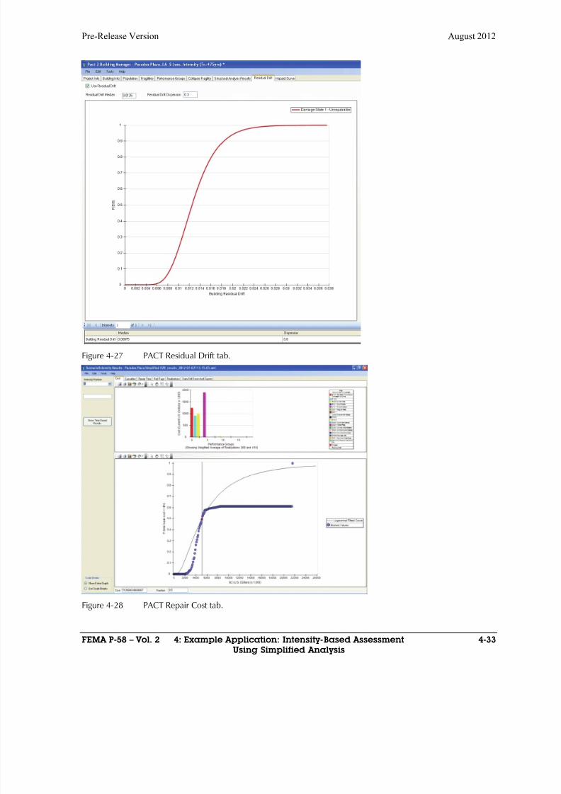
8/12/2019 Seismic Performance Assessment of Buildings
http://slidepdf.com/reader/full/seismic-performance-assessment-of-buildings 171/358
Pre-Release Version August 2012
FEMA P-58 – Vol. 2 4: Example Application: Intensity-Based Assessment 4-33
Using Simplified Analysis
Figure 4-27 PACT Residual Drift tab.
Figure 4-28 PACT Repair Cost tab.
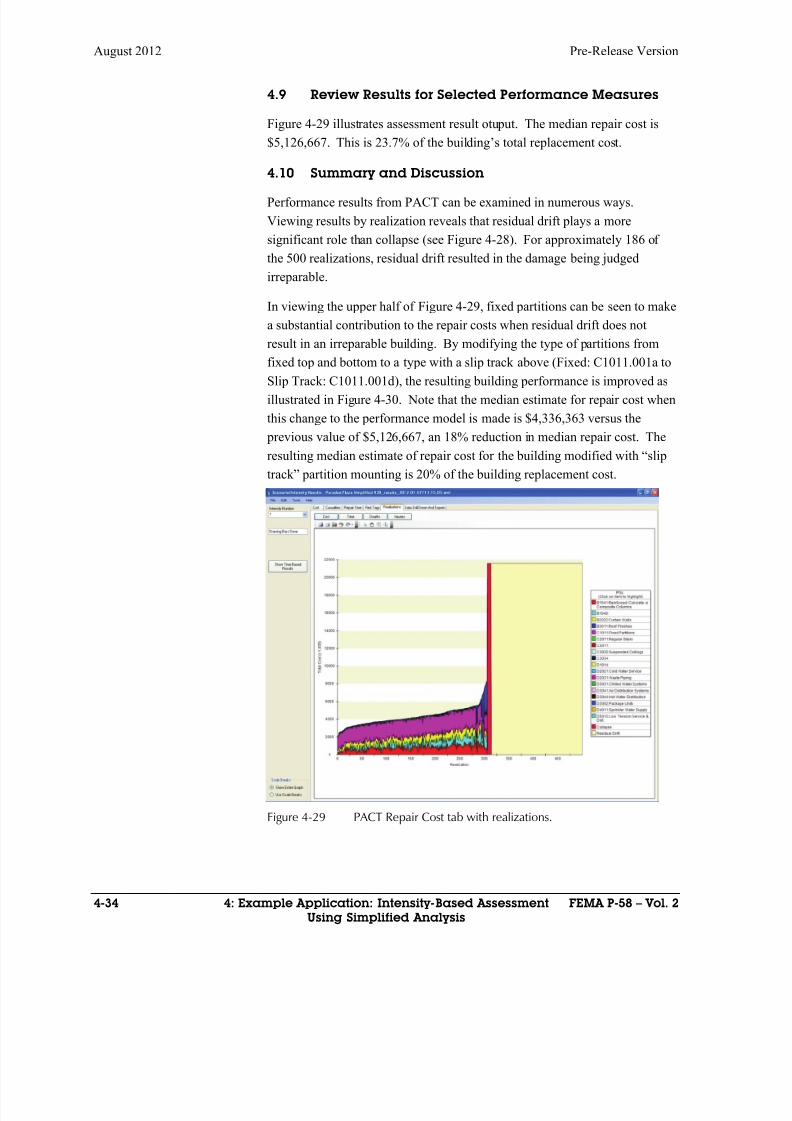
8/12/2019 Seismic Performance Assessment of Buildings
http://slidepdf.com/reader/full/seismic-performance-assessment-of-buildings 172/358

8/12/2019 Seismic Performance Assessment of Buildings
http://slidepdf.com/reader/full/seismic-performance-assessment-of-buildings 173/358
Pre-Release Version August 2012
FEMA P-58 – Vol. 2 4: Example Application: Intensity-Based Assessment 4-35
Using Simplified Analysis
Figure 4-30 PACT Repair Cost tab for results with slip track partitions.
In summary, estimated median repair cost for the 4 story reinforced concrete
building in Los Angeles, when subjected to an intensity of ground shaking
that has a mean return period of 475 years is 23.7% of the building
replacement cost. By incorporating slip track mounting to the interior
partitions, the median repair cost estimate can be reduced to 20% of the
replacement cost.

8/12/2019 Seismic Performance Assessment of Buildings
http://slidepdf.com/reader/full/seismic-performance-assessment-of-buildings 174/358
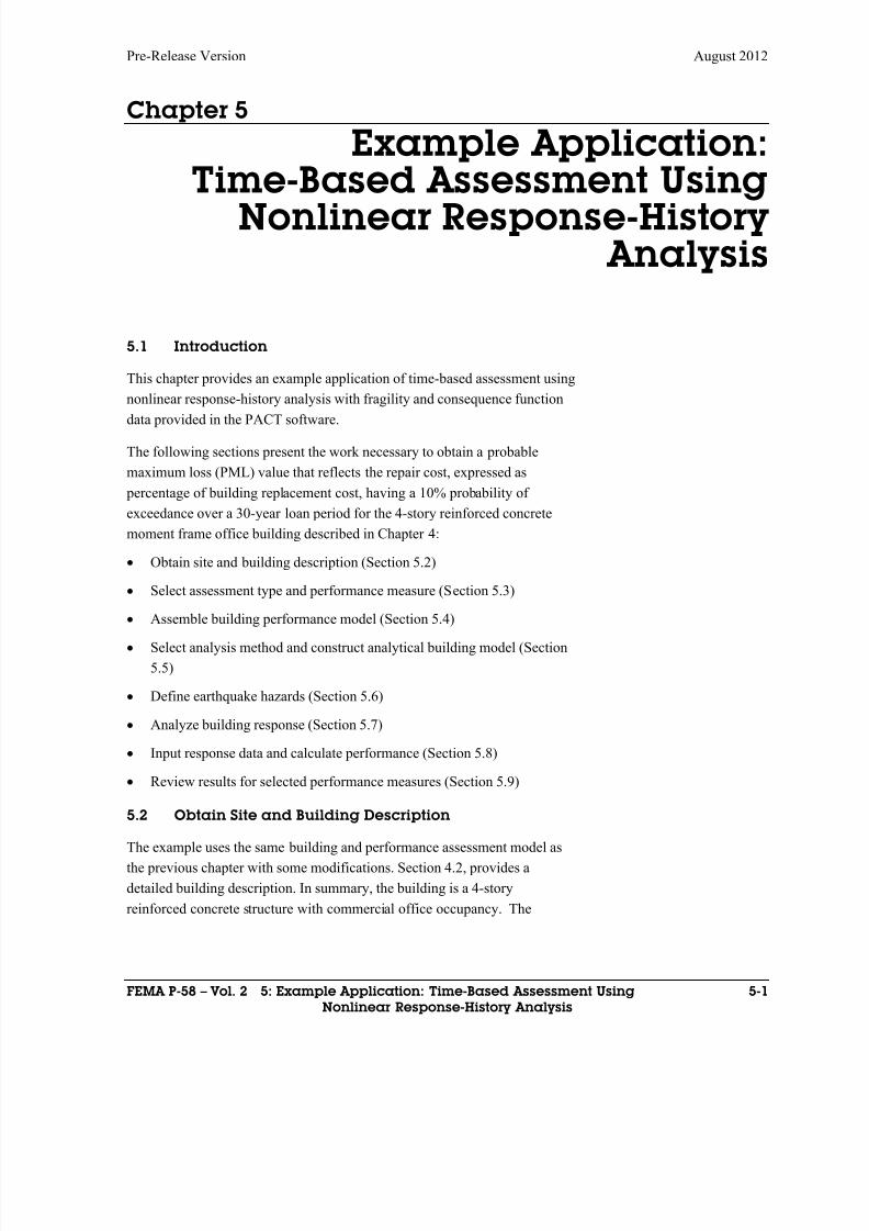
8/12/2019 Seismic Performance Assessment of Buildings
http://slidepdf.com/reader/full/seismic-performance-assessment-of-buildings 175/358
Pre-Release Version August 2012
FEMA P-58 – Vol. 2 5: Example Application: Time-Based Assessment Using 5-1
Nonlinear Response-History Analysis
Chapter 5
Example Application:Time-Based Assessment Using
Nonlinear Response-History Analysis
5.1 Introduction
This chapter provides an example application of time-based assessment using
nonlinear response-history analysis with fragility and consequence functiondata provided in the PACT software.
The following sections present the work necessary to obtain a probable
maximum loss (PML) value that reflects the repair cost, expressed as
percentage of building replacement cost, having a 10% probability of
exceedance over a 30-year loan period for the 4-story reinforced concrete
moment frame office building described in Chapter 4:
Obtain site and building description (Section 5.2)
Select assessment type and performance measure (Section 5.3)
Assemble building performance model (Section 5.4)
Select analysis method and construct analytical building model (Section
5.5)
Define earthquake hazards (Section 5.6)
Analyze building response (Section 5.7)
Input response data and calculate performance (Section 5.8)
Review results for selected performance measures (Section 5.9)
5.2 Obtain Site and Building Description
The example uses the same building and performance assessment model as
the previous chapter with some modifications. Section 4.2, provides a
detailed building description. In summary, the building is a 4-story
reinforced concrete structure with commercial office occupancy. The
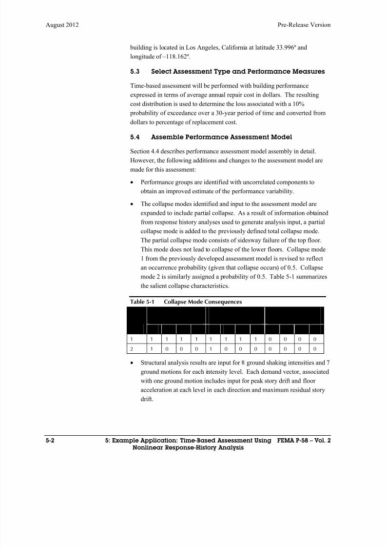
8/12/2019 Seismic Performance Assessment of Buildings
http://slidepdf.com/reader/full/seismic-performance-assessment-of-buildings 176/358
8/12/2019 Seismic Performance Assessment of Buildings
http://slidepdf.com/reader/full/seismic-performance-assessment-of-buildings 177/358
Pre-Release Version August 2012
FEMA P-58 – Vol. 2 5: Example Application: Time-Based Assessment Using 5-3
Nonlinear Response-History Analysis
5.5 Select Analysis Method and Construct Building
Analytical Model
The structure is analyzed using nonlinear response-history analysis. A three
dimensional analytical model is assembled as described in Section 3.2.2 and
Volume 1 Chapter 5.
5.6 Define Earthquake Hazards
Time-based assessment requires execution of the procedure presented in
Section 3.5.1. The nine steps described in that section are illustrated below
for the example building.
Step 1. In order to determine the building’s fundamental translational
periods in two orthogonal directions, modal analysis is performed. For this
doubly symmetric building 1 1 1.13 X Y T T s .
Step 2. The first mode average period is 1.13T s since T 1 X and T 1Y are
identical.
Step 3. Obtain a seismic hazard curve for .aS T While site-specific
seismic hazard analysis can be used, for this example the ground motion
calculator maintained by the United States Geologic Survey is used. The
basic information necessary to generate the seismic hazard curve using this
approach includes the site latitude and longitude (accurate to three decimal
places), the average period, T , and the site class as defined in ASCE/SEI 7-
10.
As noted in Chapter 4, the example building is located in the Los Angeles
area with: Latitude: 33.996°, Longitude: -118.162°, and ASCE-7 Site Class
D.
The USGS ground motion calculator provides spectral acceleration hazard
curves for sites conforming to ASCE/SEI 7-10 Site Class B at the following
building periods: 0, 0.1, 0.2, 0.3, 0.5, 1.0 and 2.0 seconds at the building
location. For intermediate periods, the value of S a can be determined by
constructing the spectrum using the above periods and graphically
determining the value of S a(T ). For structures in the period range of 0.7 to 2.0
seconds, it is generally considered sufficiently accurate to obtain S a(T ) from
the formula:
1.0a
a
S S T
T
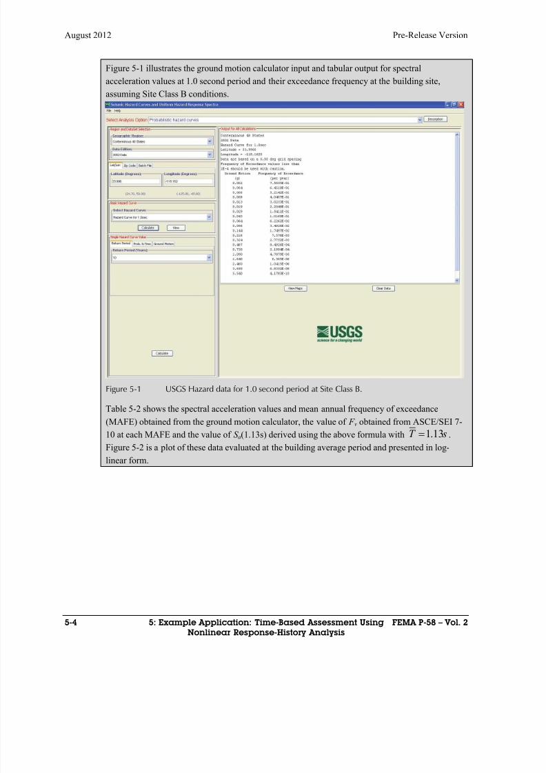
8/12/2019 Seismic Performance Assessment of Buildings
http://slidepdf.com/reader/full/seismic-performance-assessment-of-buildings 178/358
August 2012 Pre-Release Version
5-4 5: Example Application: Time-Based Assessment Using FEMA P-58 – Vol. 2
Nonlinear Response-History Analysis
Figure 5-1 illustrates the ground motion calculator input and tabular output for spectral
acceleration values at 1.0 second period and their exceedance frequency at the building site,
assuming Site Class B conditions.
Figure 5-1 USGS Hazard data for 1.0 second period at Site Class B.
Table 5-2 shows the spectral acceleration values and mean annual frequency of exceedance
(MAFE) obtained from the ground motion calculator, the value of F v obtained from ASCE/SEI 7-
10 at each MAFE and the value of S a(1.13s) derived using the above formula with sT 13.1 .
Figure 5-2 is a plot of these data evaluated at the building average period and presented in log-
linear form.
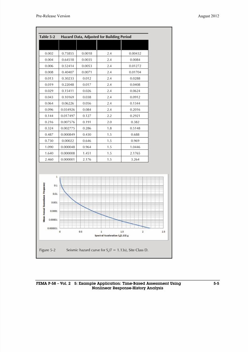
8/12/2019 Seismic Performance Assessment of Buildings
http://slidepdf.com/reader/full/seismic-performance-assessment-of-buildings 179/358
Pre-Release Version August 2012
FEMA P-58 – Vol. 2 5: Example Application: Time-Based Assessment Using 5-5
Nonlinear Response-History Analysis
Table 5-2 Hazard Data, Adjusted for Building Period
Sa(T =1.00s)Site Class B MAFE
Sa(T =1.13s)Site Class B F
v Sa(T = 1.13s)
0.002 0.75855 0.0018 2.4 0.00432
0.004 0.64518 0.0035 2.4 0.0084
0.006 0.52414 0.0053 2.4 0.01272
0.008 0.40407 0.0071 2.4 0.01704
0.013 0.30233 0.012 2.4 0.0288
0.019 0.22048 0.017 2.4 0.0408
0.029 0.15411 0.026 2.4 0.0624
0.043 0.10169 0.038 2.4 0.0912
0.064 0.06226 0.056 2.4 0.1344
0.096 0.034926 0.084 2.4 0.2016
0.144 0.017497 0.127 2.2 0.2921
0.216 0.007576 0.191 2.0 0.382
0.324 0.002775 0.286 1.8 0.5148
0.487 0.000849 0.430 1.5 0.688
0.730 0.00022 0.646 1.5 0.969
1.090 0.000048 0.964 1.5 1.0446
1.640 0.000008 1.451 1.5 2.1765
2.460 0.000001 2.176 1.5 3.264
Figure 5-2 Seismic hazard curve for Sa(T = 1.13s), Site Class D.
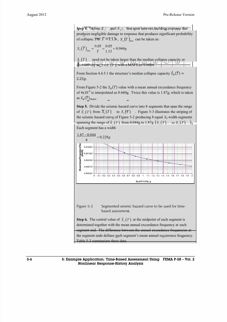
8/12/2019 Seismic Performance Assessment of Buildings
http://slidepdf.com/reader/full/seismic-performance-assessment-of-buildings 180/358
August 2012 Pre-Release Version
5-6 5: Example Application: Time-Based Assessment Using FEMA P-58 – Vol. 2
Nonlinear Response-History Analysis
Step 4. DefineminaS and
maxaS that span between building response that
produces negligible damage to response that produces significant probability
of collapse. For sT 13.1 , minT S a can be taken as:
min
0.05 0.050.044
1.13
aS T g
T
maxa
S T need not be taken larger than the median collapse capacity or
alternatively as 2a
S T with a MAFE of 0.0004.
From Section 4.4.5.1 the structure’s median collapse capacity
2.23.
From Figure 5-2 the value with a mean annual exceedance frequency
of 4x10⁻⁴ is interpolated as 0.660g. Twice this value is 1.87g, which is taken
as .
Step 5. Divide the seismic hazard curve into 8 segments that span the range
of aS T from
minaS T to maxaS T . Figure 5-3 illustrates the striping of
the seismic hazard curve of Figure 5-2 producing 8 equal S a-width segments
spanning the range of aS T from 0.044g to 1.87g min maxa a
S T to S T .
Each segment has a width
1.87 0.0440.228
8 g
Figure 5-3 Segmented seismic hazard curve to be used for time-
based assessment.
Step 6. The central value of aS T at the midpoint of each segment is
determined together with the mean annual exceedance frequency at each
segment end. The difference between the annual exceedance frequencies at
the segment ends defines each segment’s mean annual occurrence frequency.
Table 5-3 summarizes these data.

8/12/2019 Seismic Performance Assessment of Buildings
http://slidepdf.com/reader/full/seismic-performance-assessment-of-buildings 181/358
Pre-Release Version August 2012
FEMA P-58 – Vol. 2 5: Example Application: Time-Based Assessment Using 5-7
Nonlinear Response-History Analysis
Table 5-3 Intensity Segment Values
SpectralSegment ia
S ja
S aS
Δλ
(MAFE)
1 0.044 0.272 0.158 0.025
2 0.272 0.500 0.387 0.0047
3 0.500 0.729 0.615 0.0016
4 0.729 0.957 0.843 0.00064
5 0.957 1.186 1.071 0.00032
6 1.186 1.414 1.299 0.00017
7 1.414 1.640 1.528 0.00010
8 1.640 1.870 1.756 0.00005
Step 7. For each intensity segment, construct a response spectrum used for the
ground motion scaling of Step 8. For this example, uniform hazard spectra are used
for segments 1 and 2, which have mean annual return periods (inverse of MAFE) of
11.2 and 152.1 years respectively. For segments 3 through 8, conditional mean
spectra are used.
Construction of uniform hazard spectra for segments 1 and 2 is accomplished using
the same USGS ground motion calculator. This calculator can develop uniform
hazard spectra having probabilities of exceedance of 10% in 50 years of 2% in 50
years for Site Class B. Figure 5-4 illustrates such a spectrum generated for the site
coordinates of this example. Note that if the site corresponds to a Site Class other
than Site Class B, it will be necessary to convert this spectrum to the appropriate siteclass using the site adjustment factors F a and F v obtained from ASCE/SEI 7-10. The
adjusted spectral shape can be considered constant for MAFE’s ranging up to perhaps
0.001. For less frequent intensities, see ASCE/SEI 41-06 Section 1.6 for hazard
spectral adjustments.
To generate conditional mean spectra for the remaining segments, the dominant
contributor to T S a for each segment must be defined in terms of magnitude, M ,
site-to-source distance, R, and ε attributes. Deaggregation of the seismic hazard can
be done for each intensity interval for selected structural periods and annual
exceedance frequencies using an online seismic hazard deaggregation toolmaintained by the USGS. The tool can provide the dominant R, M , ε attributes at
periods of 0, 0.1, 0.2, 0.3, 0.5, 1.0, 2.0, 3.0, 4.0, and 5.0 seconds for selected
combinations of ground motion exceedance probability (1%, 2%, 5%, 10%, 20%, and
50%) and time periods (30, 50, 75, 100, and 200 years). To obtain mean annual
frequency of exceedance divide the exceedance probability (e.g., 20%) by the
number of years (e.g., 75). In this example the MAFE corresponding with a 20%
chance of exceedance in 75 years is:

8/12/2019 Seismic Performance Assessment of Buildings
http://slidepdf.com/reader/full/seismic-performance-assessment-of-buildings 182/358
August 2012 Pre-Release Version
5-8 5: Example Application: Time-Based Assessment Using FEMA P-58 – Vol. 2
Nonlinear Response-History Analysis
0.20.0027
75 MAFE
Figure 5-4 Uniform Hazard Spectrum.
Table 5-4 summarizes deaggregation results for segments 3 through 8. Figure
5-5 illustrates a sample deaggregation for segment 3. This tool can also be
used to directly generate conditional mean spectra from the deaggragation
information.
Table 5-5 Deaggregation Summary
Segment aS MAFE M R
3 0.615 0.0016 6.9 18 0.9
4 0.843 0.00064 6.9 18 1.5
5 1.071 0.00032 6.9 13 1.6
6 1.299 0.00017 6.8 10 1.7
7 1.528 0.00010 6.8 8 1.7
8 1.756 0.00005 6.8 7 1.8
These data can be used to construct a conditional mean spectrum for each
intensity segment. Figure 5-6 illustrates the conditional mean spectrum
generated for segment 3 by the USGS calculator.
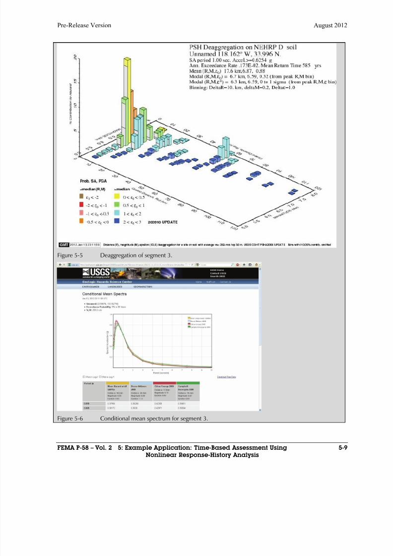
8/12/2019 Seismic Performance Assessment of Buildings
http://slidepdf.com/reader/full/seismic-performance-assessment-of-buildings 183/358
Pre-Release Version August 2012
FEMA P-58 – Vol. 2 5: Example Application: Time-Based Assessment Using 5-9
Nonlinear Response-History Analysis
Figure 5-5 Deaggregation of segment 3.
Figure 5-6 Conditional mean spectrum for segment 3.
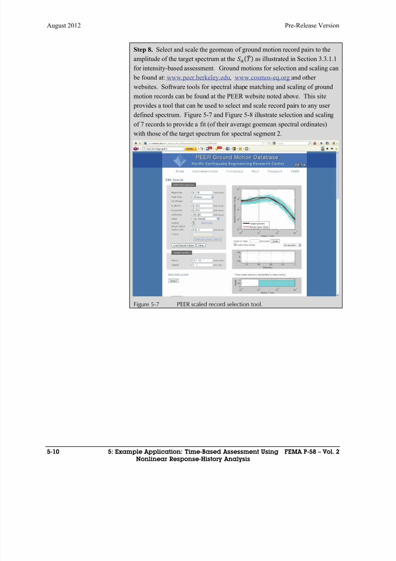
8/12/2019 Seismic Performance Assessment of Buildings
http://slidepdf.com/reader/full/seismic-performance-assessment-of-buildings 184/358
August 2012 Pre-Release Version
5-10 5: Example Application: Time-Based Assessment Using FEMA P-58 – Vol. 2
Nonlinear Response-History Analysis
Step 8. Select and scale the geomean of ground motion record pairs to the
amplitude of the target spectrum at the as illustrated in Section 3.3.1.1
for intensity-based assessment. Ground motions for selection and scaling can
be found at: www.peer.berkeley.edu, www.cosmos-eq.org and other
websites. Software tools for spectral shape matching and scaling of ground
motion records can be found at the PEER website noted above. This site
provides a tool that can be used to select and scale record pairs to any user
defined spectrum. Figure 5-7 and Figure 5-8 illustrate selection and scaling
of 7 records to provide a fit (of their average goemean spectral ordinates)
with those of the target spectrum for spectral segment 2.
Figure 5-7 PEER scaled record selection tool.
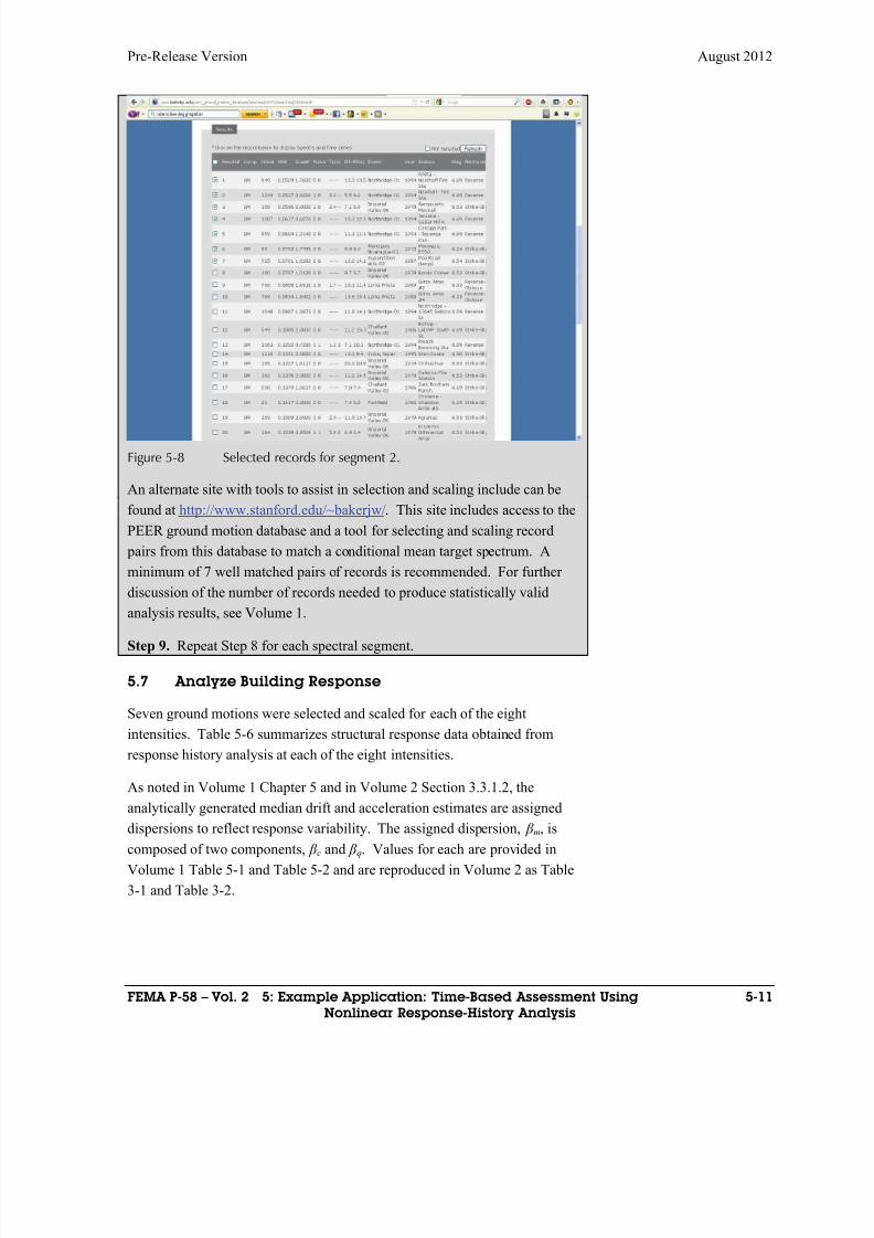
8/12/2019 Seismic Performance Assessment of Buildings
http://slidepdf.com/reader/full/seismic-performance-assessment-of-buildings 185/358
Pre-Release Version August 2012
FEMA P-58 – Vol. 2 5: Example Application: Time-Based Assessment Using 5-11
Nonlinear Response-History Analysis
Figure 5-8 Selected records for segment 2.
An alternate site with tools to assist in selection and scaling include can be
found at http://www.stanford.edu/~bakerjw/. This site includes access to the
PEER ground motion database and a tool for selecting and scaling record
pairs from this database to match a conditional mean target spectrum. A
minimum of 7 well matched pairs of records is recommended. For further
discussion of the number of records needed to produce statistically valid
analysis results, see Volume 1.
Step 9. Repeat Step 8 for each spectral segment.
5.7 Analyze Building Response
Seven ground motions were selected and scaled for each of the eight
intensities. Table 5-6 summarizes structural response data obtained from
response history analysis at each of the eight intensities.
As noted in Volume 1 Chapter 5 and in Volume 2 Section 3.3.1.2, the
analytically generated median drift and acceleration estimates are assigneddispersions to reflect response variability. The assigned dispersion, β m, is
composed of two components, β c and β q. Values for each are provided in
Volume 1 Table 5-1 and Table 5-2 and are reproduced in Volume 2 as Table
3-1 and Table 3-2.

8/12/2019 Seismic Performance Assessment of Buildings
http://slidepdf.com/reader/full/seismic-performance-assessment-of-buildings 186/358
August 2012 Pre-Release Version
5-12 5: Example Application: Time-Based Assessment Using FEMA P-58 – Vol. 2
Nonlinear Response-History Analysis
Table 5-6 Summary of Structural Analysis Results
Intensity 1 Sa( )=0.158 g Intensity 2 Sa( )=0.387 g
DemandParameter
Median Parameter Median
Δ4 0.002 Δ4 0.003
Δ3 0.004 Δ3 0.008
Δ2 0.005 Δ2 0.0134
Δ1 0.005 Δ1 0.010
a5 0.24 a5 0.34
a4 0.18 a4 0.30
a3 0.19 a3 0.30
a2 0.16 a2 0.30
a1 0.19 a1 0.22
Intensity 3 Sa( )=0.615 g Intensity 4 Sa( )=0.843 g
Demand
Parameter Median Parameter Median
Δ4 0.006 Δ4 0.008
Δ3 0.013 Δ3 0.019
Δ2 0.017 Δ2 0.024
Δ1 0.015 Δ1 0.022
a5 0.43 a5 0.48
a4 0.36 a4 0.41
a3 0.38 a3 0.48
a2 0.43 a2 0.53
a1 0.36 a1 0.48
Intensity 5 Sa( )=1.071 g Intensity 6 Sa( )=1.299 g
DemandParameter
Median Parameter Median
Δ4 0.012 Δ4 0.011
Δ3 0.024 Δ3 0.025
Δ2 0.030 Δ2 0.039
Δ1 0.029 Δ1 0.037
a5 0.49 a5 0.55
a4 0.44 a4 0.45
a3 0.48 a3 0.52
a2 0.59 a2 0.69
a1 0.52 a1 0.68
Δi: Maximum drift ratio at story i
ai: Peak floor acceleration at floor i
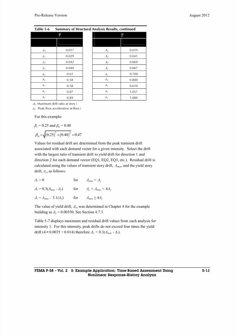
8/12/2019 Seismic Performance Assessment of Buildings
http://slidepdf.com/reader/full/seismic-performance-assessment-of-buildings 187/358
Pre-Release Version August 2012
FEMA P-58 – Vol. 2 5: Example Application: Time-Based Assessment Using 5-13
Nonlinear Response-History Analysis
Table 5-6 Summary of Structural Analysis Results, continued
Intensity 7 Sa( )=1.528 g Intensity 8 Sa( )=1.756 g
DemandParameter
MedianDemand
ParameterMedian
Δ4 0.017 Δ4 0.019
Δ3 0.029 Δ3 0.041
Δ2 0.042 Δ2 0.069
Δ1 0.040 Δ1 0.067
a5 0.61 a5 0.700
a4 0.58 a4 0.800
a3 0.58 a3 0.610
a2 0.87 a2 1.057
a1 0.89 a1 1.000
Δi: Maximum drift ratio at story i
ai: Peak floor acceleration at floor
i
For this example:
β c = 0.25 and β q = 0.40
2 2
0.25 0.40 0.47m
Values for residual drift are determined from the peak transient drift
associated with each demand vector for a given intensity. Select the drift
with the largest ratio of transient drift to yield drift for direction 1 and
direction 2 for each demand vector (EQ1, EQ2, EQ3, etc.). Residual drift is
calculated using the values of transient story drift, Δmax, and the yield storydrift, Δ y, as follows:
Δr = 0 for Δmax < Δ y
Δr = 0.3( Δmax - Δ y) for Δ y < Δmax < 4 Δ y
Δr = Δmax – 3.1( Δ y) for Δmax ≥ 4 Δ y
The value of yield drift, Δ y, was determined in Chapter 4 for the example
building as Δ y = 0.00350. See Section 4.7.3.
Table 5-7 displays maximum and residual drift values from each analysis forintensity 1. For this intensity, peak drifts do not exceed four times the yield
drift (4 0.0035 = 0.014) therefore Δr = 0.3( Δmax - Δr ).
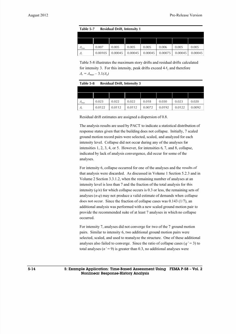
8/12/2019 Seismic Performance Assessment of Buildings
http://slidepdf.com/reader/full/seismic-performance-assessment-of-buildings 188/358
August 2012 Pre-Release Version
5-14 5: Example Application: Time-Based Assessment Using FEMA P-58 – Vol. 2
Nonlinear Response-History Analysis
Table 5-7 Residual Drift, Intensity 1
Intensity 1: Sa = 0.158g
1 2 3 4 5 6 7
Δmax 0.007 0.005 0.005 0.005 0.006 0.005 0.005
Δr
0.00105 0.00045 0.00045 0.00045 0.00075 0.00045 0.00045
Table 5-8 illustrates the maximum story drifts and residual drifts calculated
for intensity 3. For this intensity, peak drifts exceed 4 Δ y and therefore
Δr = Δmax – 3.1( Δ y )
Table 5-8 Residual Drift, Intensity 3
Intensity 3: Sa = 0.615g
1 2 3 4 5 6 7
Δmax 0.023 0.022 0.022 0.018 0.030 0.023 0.020
Δr 0.0122 0.0112 0.0112 0.0072 0.0192 0.0122 0.0092
Residual drift estimates are assigned a dispersion of 0.8.
The analysis results are used by PACT to indicate a statistical distribution of
response states given that the building does not collapse. Initially, 7 scaled
ground motion record pairs were selected, scaled, and analyzed for each
intensity level. Collapse did not occur during any of the analyses for
intensities 1, 2, 3, 4, or 5. However, for intensities 6, 7, and 8, collapse,
indicated by lack of analysis convergence, did occur for some of the
analyses.
For intensity 6, collapse occurred for one of the analyses and the results of
that analysis were discarded. As discussed in Volume 1 Section 5.2.3 and in
Volume 2 Section 3.3.1.2, when the remaining number of analyses at an
intensity level is less than 7 and the fraction of the total analysis for this
intensity (q/n) for which collapse occurs is 0.3 or less, the remaining sets of
analyses (n-q) may not produce a valid estimate of demands when collapse
does not occur. Since the fraction of collapse cases was 0.143 (1/7), an
additional analysis was performed with a new scaled ground motion pair to
provide the recommended suite of at least 7 analyses in which no collapse
occurred.
For intensity 7, analyses did not converge for two of the 7 ground motion
pairs. Similar to intensity 6, two additional ground motion pairs were
selected, scaled, and used to reanalyze the structure. One of these additional
analyses also failed to converge. Since the ratio of collapse cases (q’ = 3) to
total analyses (n’ = 9) is greater than 0.3, no additional analyses were

8/12/2019 Seismic Performance Assessment of Buildings
http://slidepdf.com/reader/full/seismic-performance-assessment-of-buildings 189/358
Pre-Release Version August 2012
FEMA P-58 – Vol. 2 5: Example Application: Time-Based Assessment Using 5-15
Nonlinear Response-History Analysis
performed and the 6 records that did not produce collapse were used to
establish the median demand values for this intensity segment.
For intensity 8, three of the 7 ground motion record pairs produced collapse.
Since the ratio of collapse cases (q = 3) to total number of analyses (n = 7)
exceeds 0.3, no additional analyses were performed and the 4 records that didnot produce collapse were entered into PACT.
5.8 Input Response Data and Calculate Performance
Structural analysis results for each of the 8 intensity levels are input to PACT
on the Structural Analysis Results tab. Figure 5-9 illustrates the drift input
values for intensity 3, direction 1 and direction 2. Input includes spectral
acceleration (S a = 0.615g), dispersion ( β m = 0.47) and includes input for all 7
demand vectors. Peak floor accelerations are input similarly.
Figure 5-9 PACT Structural Analysis Results tab with drift input for intensity 3.
Peak residual drift values are input via the Residual Drift tab. Figure 5-10
illustrates this input for intensity 3. The residual drift fragility information in
the upper portion of the screen remains the same as in the previousassessment model developed in Chapter 4 (median value of 0.0125 and a
dispersion of 0.3).
The MAFE values corresponding to each of the intensities is input via the
Hazard Curve tab. Figure 5-11 illustrates input of this information.
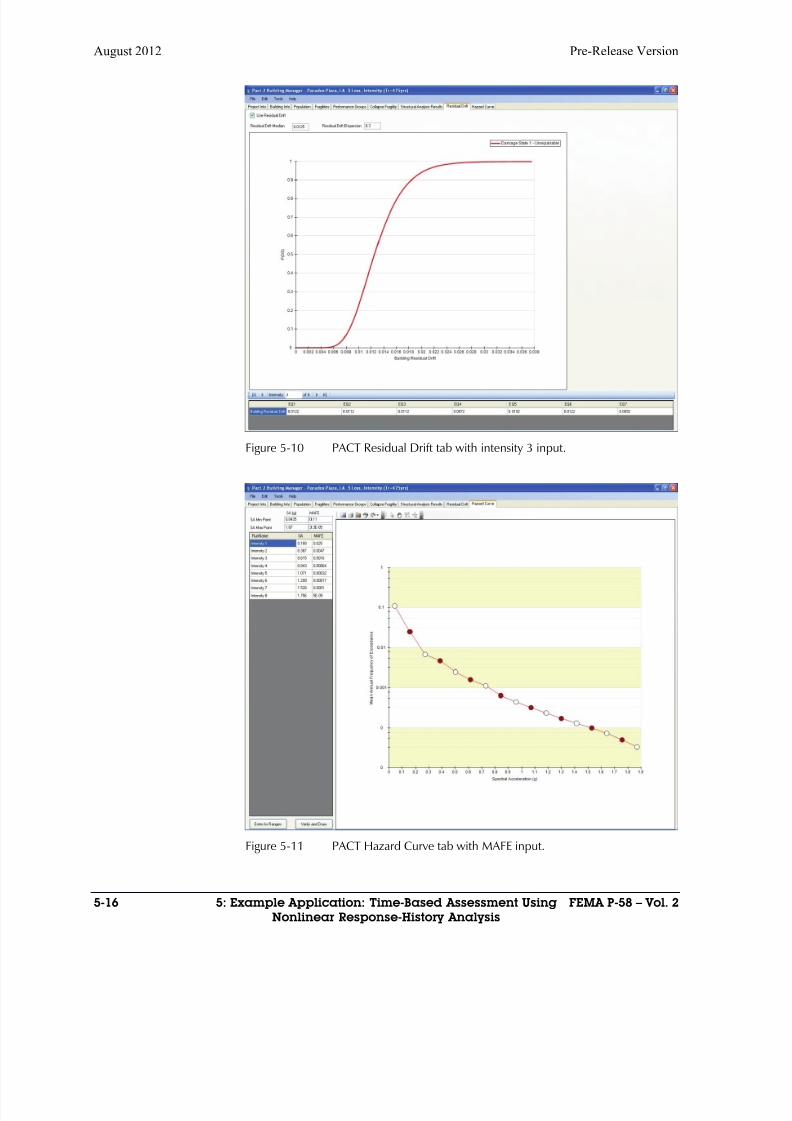
8/12/2019 Seismic Performance Assessment of Buildings
http://slidepdf.com/reader/full/seismic-performance-assessment-of-buildings 190/358
August 2012 Pre-Release Version
5-16 5: Example Application: Time-Based Assessment Using FEMA P-58 – Vol. 2
Nonlinear Response-History Analysis
Figure 5-10 PACT Residual Drift tab with intensity 3 input.
Figure 5-11 PACT Hazard Curve tab with MAFE input.
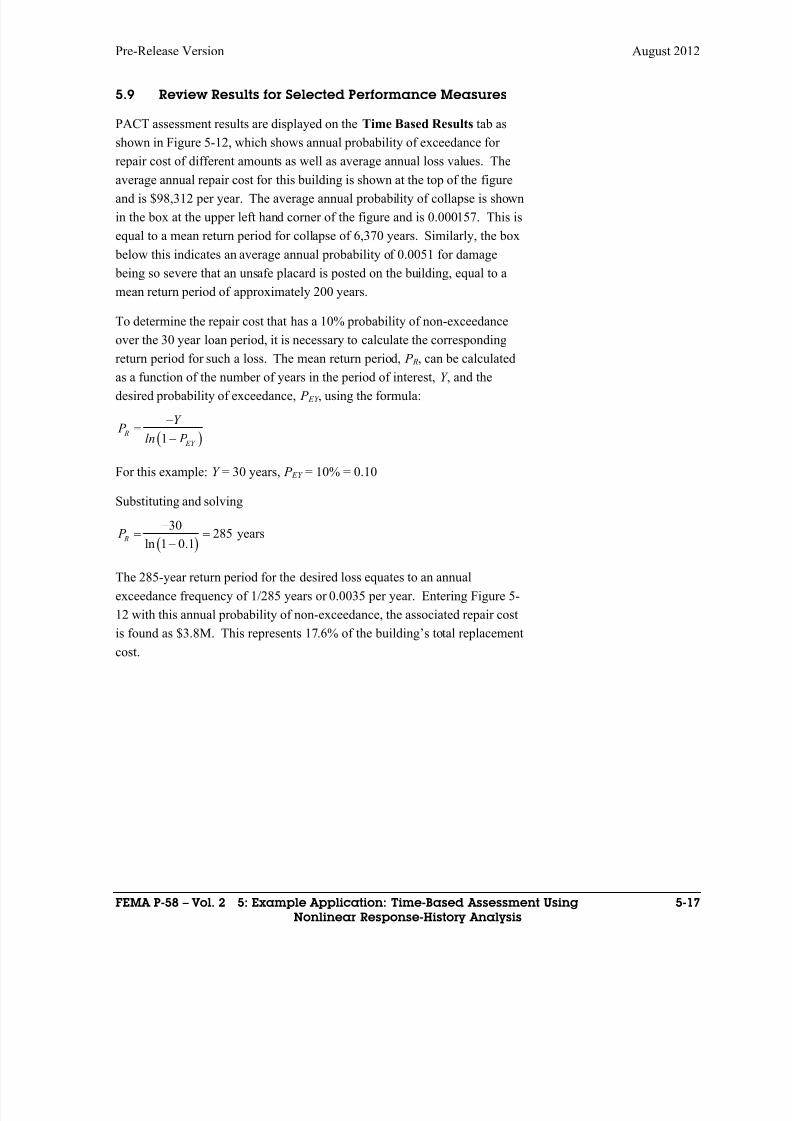
8/12/2019 Seismic Performance Assessment of Buildings
http://slidepdf.com/reader/full/seismic-performance-assessment-of-buildings 191/358
Pre-Release Version August 2012
FEMA P-58 – Vol. 2 5: Example Application: Time-Based Assessment Using 5-17
Nonlinear Response-History Analysis
5.9 Review Results for Selected Performance Measures
PACT assessment results are displayed on the Time Based Results tab as
shown in Figure 5-12, which shows annual probability of exceedance for
repair cost of different amounts as well as average annual loss values. The
average annual repair cost for this building is shown at the top of the figureand is $98,312 per year. The average annual probability of collapse is shown
in the box at the upper left hand corner of the figure and is 0.000157. This is
equal to a mean return period for collapse of 6,370 years. Similarly, the box
below this indicates an average annual probability of 0.0051 for damage
being so severe that an unsafe placard is posted on the building, equal to a
mean return period of approximately 200 years.
To determine the repair cost that has a 10% probability of non-exceedance
over the 30 year loan period, it is necessary to calculate the corresponding
return period for such a loss. The mean return period, P R, can be calculated
as a function of the number of years in the period of interest, Y , and the
desired probability of exceedance, P EY , using the formula:
1 R
EY
Y P
ln P
For this example: Y = 30 years, P EY = 10% = 0.10
Substituting and solving
30285 years
ln 1 0.1 R P
The 285-year return period for the desired loss equates to an annual
exceedance frequency of 1/285 years or 0.0035 per year. Entering Figure 5-
12 with this annual probability of non-exceedance, the associated repair cost
is found as $3.8M. This represents 17.6% of the building’s total replacement
cost.
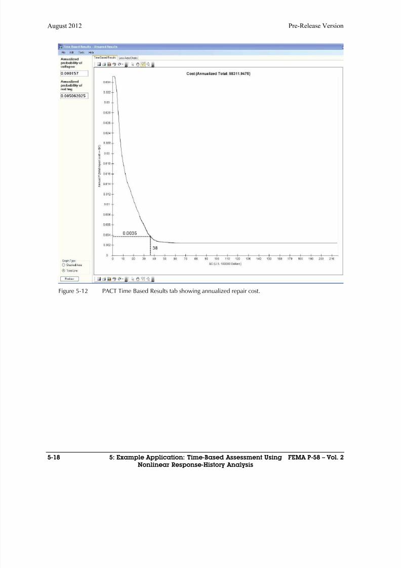
8/12/2019 Seismic Performance Assessment of Buildings
http://slidepdf.com/reader/full/seismic-performance-assessment-of-buildings 192/358
August 2012 Pre-Release Version
5-18 5: Example Application: Time-Based Assessment Using FEMA P-58 – Vol. 2
Nonlinear Response-History Analysis
Figure 5-12 PACT Time Based Results tab showing annualized repair cost.
8/12/2019 Seismic Performance Assessment of Buildings
http://slidepdf.com/reader/full/seismic-performance-assessment-of-buildings 193/358
Pre-Release Version August 2012
FEMA P-58 – Vol. 2 6: Structural Fragility Calculation 6-1
Chapter 6
Structural Fragility Calculation
6.1 Introduction
Volume 1, Section 3.8.4 and Appendix H present procedures for analytical
derivation of component fragility functions. This chapter illustrates those
procedures using a sample tilt-up concrete building comprised of a plywood
diaphragm, wood framed roofing and reinforced concrete walls. The
examples illustrate application of the procedures for ductility-limited damage
states and strength-limited damage states (ductile and brittle). The examples
provide insight into the process of selecting damage states and demand
parameters to characterize component performance. The following structural
components and systems are addressed:
Plywood diaphragms
Tilt-up concrete walls
Wall/roof attachment (in-plane)
Wall/roof attachments (out-of-plane)
By applying the procedures illustrated here, users can apply the methodology
to include structures that have components for which there are no providedfragility specifications. Chapter 7 provides guidance on the development of
nonstructural component fragility functions by calculation.
6.2 Building Description
The example structure defined below is used to illustrate the calculation of
various component fragility functions. The structure is of conventional tilt-
up concrete construction with a plywood roof diaphragm. Figure 6-1 is a
roof plan for the structure and Figure 6-2 a cross sectional elevation. Table
6-1 defines basic structural data.
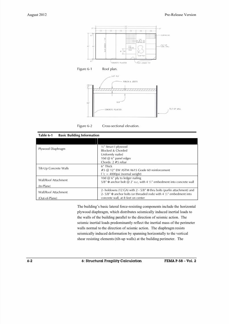
8/12/2019 Seismic Performance Assessment of Buildings
http://slidepdf.com/reader/full/seismic-performance-assessment-of-buildings 194/358
August 2012 Pre-Release Version
6-2 6: Structural Fragility Calculation FEMA P-58 – Vol. 2
Figure 6-1 Roof plan.
Figure 6-2 Cross-sectional elevation.
Table 6-1 Basic Building Information
Building Components Details of Construction
Plywood Diaphragm½” Struct I plywoodBlocked & ChordedUniformly nailed
10d @ 6” panel edgesChords: 2 #5 rebar
Tilt-Up Concrete Walls6” Thick#5 @ 12” EW ASTM A615 Grade 60 reinforcementf ’c = 4000psi (normal weight)
Wall/Roof Attachment
(In-Plane)
10d @ 6” ply to ledger nailing5/8” Φ anchor bolt @ 2’ o.c, with 4 ½” embedment into concrete wall
Wall/Roof Attachment
(Out-of-Plane)
2- holdowns (12 GA) with 2 - 5/8” Φ thru bolts (purlin attachment) and2- 5/8” Φ anchor bolts (or threaded rods) with 4 ½” embedment intoconcrete wall, at 8 feet on center
The building’s basic lateral force-resisting components include the horizontal
plywood diaphragm, which distributes seismically induced inertial loads tothe walls of the building parallel to the direction of seismic action. The
seismic inertial loads predominantly reflect the inertial mass of the perimeter
walls normal to the direction of seismic action. The diaphragm resists
seismically induced deformation by spanning horizontally to the vertical
shear resisting elements (tilt-up walls) at the building perimeter. The

8/12/2019 Seismic Performance Assessment of Buildings
http://slidepdf.com/reader/full/seismic-performance-assessment-of-buildings 195/358
Pre-Release Version August 2012
FEMA P-58 – Vol. 2 6: Structural Fragility Calculation 6-3
diaphragm exhibits fundamentally the same behavior modes in each direction
of seismic demand.
The six-inch thick reinforced concrete walls act as shear walls to provide
restraint to the diaphragm for seismic forces acting parallel to the walls. For
seismic forces acting perpendicular to the walls, the walls transmit inertialreactions to the roof diaphragm and to the foundation. The attachments of
the walls to the roof transfers the diaphragm end forces along the length of
the in-plane walls and transfer the out-of-plane inertial wall loads into the
horizontal diaphragm at discrete 8-foot intervals where tension ties (2
holdown devices) are located.
Damageable components of the building’s lateral force-resisting system
include:
Plywood Roof Diaphragm
o Transverse
o Longitudinal
Tilt-Up Concrete Walls
o In-plane
o Out-of-plane
Wall/Roof Attachments
o In-plane
o Out-of-plane
The walls and roof are attached to transfer in-plane and out-of-plane wall and
diaphragm demands. The in-plane attachment (Figure 6-3) consists of a
diaphragm ledger (3x8, DF#1, timber) and steel anchor bolts that are
embedded into the concrete wall (5/8 inch diameter at 2 feet on center). The
out-of-plane attachment consists of holdown hardware (see Figure 6-4 and
Figure 6-5) attached to diaphragm sub-framing and bolted to the concrete
wall in a fashion similar to that of the in-plane connection. The sub-framing
is attached to the plywood diaphragm via nailing that provides a mechanism
for engaging the diaphragm to resist inertial wall demands. The sub-framingincludes splice detailing to maintain transfer continuity over a distance
sufficient to engage an adequate number of nails between the sub-framing
and the plywood.
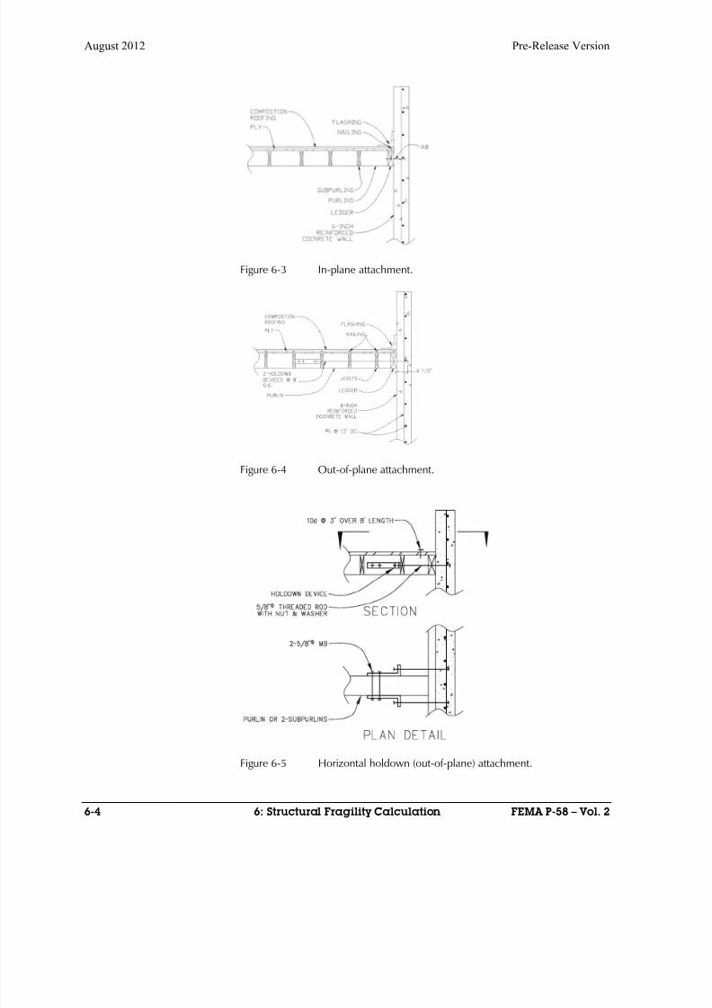
8/12/2019 Seismic Performance Assessment of Buildings
http://slidepdf.com/reader/full/seismic-performance-assessment-of-buildings 196/358
August 2012 Pre-Release Version
6-4 6: Structural Fragility Calculation FEMA P-58 – Vol. 2
Figure 6-3 In-plane attachment.
Figure 6-4 Out-of-plane attachment.
Figure 6-5 Horizontal holdown (out-of-plane) attachment.

8/12/2019 Seismic Performance Assessment of Buildings
http://slidepdf.com/reader/full/seismic-performance-assessment-of-buildings 197/358
Pre-Release Version August 2012
FEMA P-58 – Vol. 2 6: Structural Fragility Calculation 6-5
6.3 Development of Structural Component and System
Fragilities by Calculation
Volume 1, Section 3.8.4 presents procedures for calculating component
fragility functions based on characteristics of the anticipated component limit
state. Four limit state categories are identified: Strength-limited damage states
Ductility-limited damage states
Displacement-limited damage states
Code-based capacity damage states
Each limit state assumes a mathematical relationship between a demand
parameter and the occurrence of a damage state. For each category, an
estimate of the median value of the demand, θ, at which the damage state is
likely to occur is analytically estimated. It is assumed that the probability ofincurring damage at different values of demand is log-normally distributed
with dispersion, β . The value of the dispersion is selected to reflect the
variability in: component material strength, β M ; the predictive equations used
to derive the median demand estimate, β D; and the degree to which the actual
construction is likely to match the construction quality, β C , implicit in the
median demand calculation. These procedures are illustrated with the
generation of fragility functions for the components and systems of the
example building.
6.3.1 Plywood Roof Diaphragm
The plywood roof diaphragm is considered to include composition roofing
and flashing, plywood sheathing, nailing attachment to the sub-framing, and
chord and collector elements.
The diaphragm can sustain consequential damage in the following ways:
Nail pullout at plywood panel edges or buckling of plywood panels
Chord or collector buckling
Chord or collector splice failure in tension.
In this example, there are no collectors because the walls and diaphragm are
continuously attached. The chords consist of reinforcing steel embedded in
the concrete perimeter walls. These chords are unlikely to buckle or fail in a
consequential fashion for this building system given the relative vulnerability
of the wood framing components. Therefore, potential damage states
associated with the chords are not addressed in this example.

8/12/2019 Seismic Performance Assessment of Buildings
http://slidepdf.com/reader/full/seismic-performance-assessment-of-buildings 198/358
August 2012 Pre-Release Version
6-6 6: Structural Fragility Calculation FEMA P-58 – Vol. 2
Figure 6-6 Plywood diaphragm damage (Tissel, 1967).
Figure 6-7 Plywood diaphragm damage (Tissel, 1967).
A fragility function for plywood diaphragm damage states consisting of nail
pullout and panel buckling damage mechanisms is generated by calculation
using the methodology Volume 1.
Testing and observation of the performance of plywood diaphragm systems
(Tissel, 1967) suggests damage states of substance include nail pullout and
panel buckling (Figure 6-6 and Figure 6-7). Anticipated horizontal
diaphragm performance can be characterized using the generalized force-
deformation “backbone” relationship as defined in ASCE/SEI 41-06 (ASCE,
2007) and as shown in Figure 6-8 below:

8/12/2019 Seismic Performance Assessment of Buildings
http://slidepdf.com/reader/full/seismic-performance-assessment-of-buildings 199/358
Pre-Release Version August 2012
FEMA P-58 – Vol. 2 6: Structural Fragility Calculation 6-7
N o r m a l i z i e d F o r c e : Q / Q y
Normalized Displacement: Δ/Δy
Figure 6-8 Generalized component force-deformation relationship (ASCE/SEI 41-06).
ASCE/SEI 41-06 Table 8-4 lists response modeling parameters d, e and c as
4, 5, and 0.3, respectively since the subject diaphragm has a span-to-depth
ratio of approximately 3 to 1 and is blocked and chorded. ASCE 41-06 also
provides response values that are judged to reflect three levels of component
performance: Immediate Occupancy, Life Safety and Collapse Prevention.
ASCE/SEI 41-06 Table C1-4 provides a qualitative description of the
anticipated degree of damage associated with each of these response levels.
For Immediate Occupancy performance, no observable loosening or
withdrawal of fasteners is expected and no splitting of sheathing or framing
is anticipated. For Life Safety performance, observable withdrawal of thefasteners is expected as well as splitting of framing, sheathing and
connections. For Collapse Prevention performance, large permanent
distortion of the diaphragm is expected. accompanied by extensive splitting
of framing, connections. and sheathing in addition to partial nail withdrawal.
For the diaphragm system in this example, three damage states of
consequence are considered. In Damage State 1 (DS1), no damage to the
plywood, nailing or framing is anticipated, but damage to the roof flashing at
the wall/diaphragm interface is expected. This damage will require removal
and reinstallation of the flashing. Additionally, tearing of roofing materials
at this interface can be expected. This damage state reflects the
characterization of non-structural damage that might be found in PACT
under roof coverings, flat roof (B301), composition roofing, however, PACT
does not contain a provided fragility specification for this component.
In the backbone curve:
Δ = Total elastic and plastic deformation
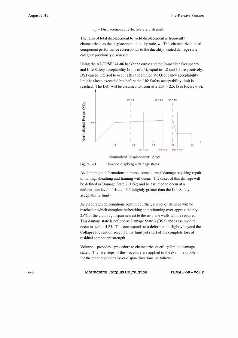
8/12/2019 Seismic Performance Assessment of Buildings
http://slidepdf.com/reader/full/seismic-performance-assessment-of-buildings 200/358
August 2012 Pre-Release Version
6-8 6: Structural Fragility Calculation FEMA P-58 – Vol. 2
Δ y = Displacement at effective yield strength
The ratio of total displacement to yield displacement is frequently
characterized as the displacement ductility ratio, μ. This characterization of
component performance corresponds to the ductility-limited damage state
category previously discussed.
Using the ASCE/SEI 41-06 backbone curve and the Immediate Occupancy
and Life Safety acceptability limits of Δ/ Δ y equal to 1.8 and 3.3, respectively,
DS1 can be inferred to occur after the Immediate Occupancy acceptability
limit has been exceeded but before the Life Safety acceptability limit is
reached. The DS1 will be assumed to occur at a Δ/ Δ y = 2.5. (See Figure 6-9).
Figure 6-9 Plywood diaphragm damage states.
As diaphragm deformations increase, consequential damage requiring repair
of nailing, sheathing and framing will occur. The onset of this damage will
be defined as Damage State 2 (DS2) and be assumed to occur at a
deformation level of Δ/ Δ y = 3.5 (slightly greater than the Life Safety
acceptability limit).
As diaphragm deformations continue further, a level of damage will be
reached at which complete resheathing and reframing over approximately
25% of the diaphragm span nearest to the in-plane walls will be required.
This damage state is defined as Damage State 3 (DS3) and is assumed tooccur at Δ/ Δ y = 4.25. This corresponds to a deformation slightly beyond the
Collapse Prevention acceptability limit yet short of the complete loss of
residual component strength.
Volume 1 provides a procedure to characterize ductility-limited damage
states. The five steps of the procedure are applied to the example problem
for the diaphragm’s transverse span directions, as follows:
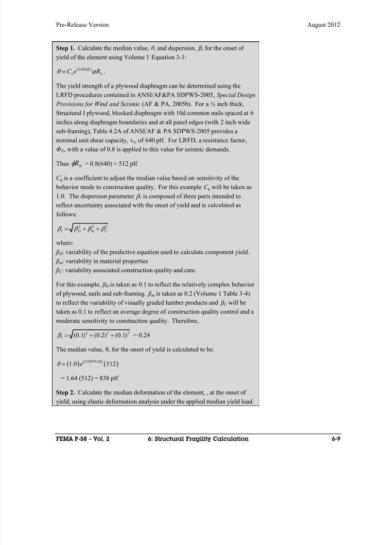
8/12/2019 Seismic Performance Assessment of Buildings
http://slidepdf.com/reader/full/seismic-performance-assessment-of-buildings 201/358
Pre-Release Version August 2012
FEMA P-58 – Vol. 2 6: Structural Fragility Calculation 6-9
Step 1. Calculate the median value, θ , and dispersion, , for the onset of
yield of the element using Volume 1 Equation 3-1:
1(2.054 )
q N C e R .
The yield strength of a plywood diaphragm can be determined using the
LRFD procedures contained in ANSI/AF&PA SDPWS-2005, Special Design
Provisions for Wind and Seismic (AF & PA, 2005b). For a ½ inch thick,
Structural I plywood, blocked diaphragm with 10d common nails spaced at 6
inches along diaphragm boundaries and at all panel edges (with 2 inch wide
sub-framing), Table 4.2A of ANSI/AF & PA SDPWS-2005 provides a
nominal unit shear capacity, v s, of 640 plf. For LRFD, a resistance factor,
Φ D, with a value of 0.8 is applied to this value for seismic demands.
Thus N R = 0.8(640) = 512 plf
C q is a coefficient to adjust the median value based on sensitivity of the behavior mode to construction quality. For this example C q will be taken as
1.0. The dispersion parameter 1 is composed of three parts intended to
reflect uncertainty associated with the onset of yield and is calculated as
follows:
2 2 2
1 D m C
where:
β D: variability of the predictive equation used to calculate component yield.
β m: variability in material properties
β C : variability associated construction quality and care.
For this example, β D is taken as 0.1 to reflect the relatively complex behavior
of plywood, nails and sub-framing. β m is taken as 0.2 (Volume 1 Table 3-4)
to reflect the variability of visually graded lumber products and β C will be
taken as 0.1 to reflect an average degree of construction quality control and a
moderate sensitivity to construction quality. Therefore,
2 2 2
1 (0.1) (0.2) (0.1) = 0.24
The median value, θ, for the onset of yield is calculated to be:
2.054*0.241.0 512e
= 1.64 (512) = 838 plf
Step 2. Calculate the median deformation of the element, , at the onset of
yield, using elastic deformation analysis under the applied median yield load.
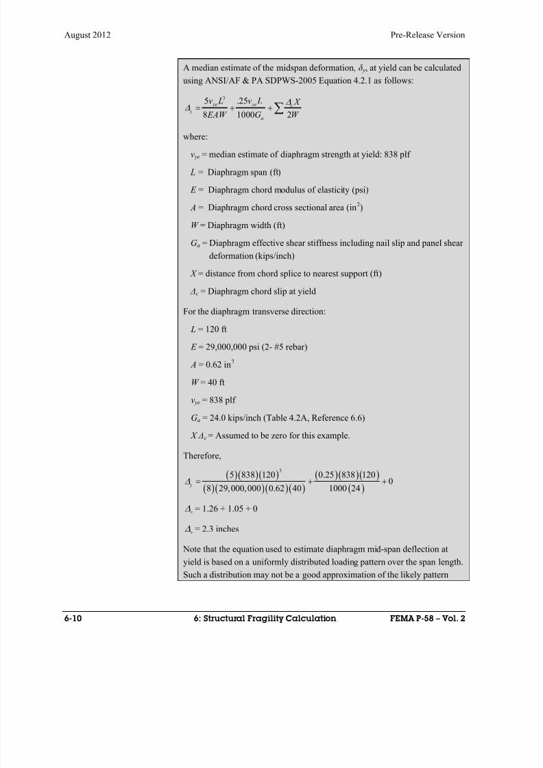
8/12/2019 Seismic Performance Assessment of Buildings
http://slidepdf.com/reader/full/seismic-performance-assessment-of-buildings 202/358
August 2012 Pre-Release Version
6-10 6: Structural Fragility Calculation FEMA P-58 – Vol. 2
A median estimate of the midspan deformation, δ y, at yield can be calculated
using ANSI/AF & PA SDPWS-2005 Equation 4.2.1 as follows:
35 .25
8 1000 2
ye ye c y
a
v L v L X
EAW G W
where:
v ye = median estimate of diaphragm strength at yield: 838 plf
L = Diaphragm span (ft)
E = Diaphragm chord modulus of elasticity (psi)
A = Diaphragm chord cross sectional area (in2)
W = Diaphragm width (ft)
Ga = Diaphragm effective shear stiffness including nail slip and panel shear
deformation (kips/inch)
X = distance from chord splice to nearest support (ft)
Δc = Diaphragm chord slip at yield
For the diaphragm transverse direction:
L = 120 ft
E = 29,000,000 psi (2- #5 rebar)
A = 0.62 in2
W = 40 ft
v ye = 838 plf
Ga = 24.0 kips/inch (Table 4.2A, Reference 6.6)
X Δc = Assumed to be zero for this example.
Therefore,
35 838 120 0.25 838 120
08 29,000,000 0.62 40 1000 24
y
y = 1.26 + 1.05 + 0
y = 2.3 inches
Note that the equation used to estimate diaphragm mid-span deflection at
yield is based on a uniformly distributed loading pattern over the span length.
Such a distribution may not be a good approximation of the likely pattern
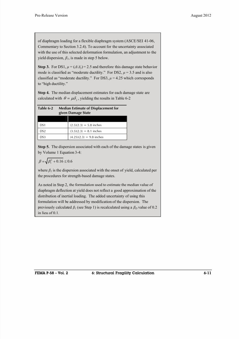
8/12/2019 Seismic Performance Assessment of Buildings
http://slidepdf.com/reader/full/seismic-performance-assessment-of-buildings 203/358
Pre-Release Version August 2012
FEMA P-58 – Vol. 2 6: Structural Fragility Calculation 6-11
of diaphragm loading for a flexible diaphragm system (ASCE/SEI 41-06,
Commentary to Section 3.2.4). To account for the uncertainty associated
with the use of this selected deformation formulation, an adjustment to the
yield dispersion, β 1, is made in step 5 below.
Step 3. For DS1, μ = ( Δ/ Δ y) = 2.5 and therefore this damage state behavior
mode is classified as “moderate ductility.” For DS2, μ = 3.5 and is also
classified as “moderate ductility.” For DS3, μ = 4.25 which corresponds
to “high ductility.”
Step 4. The median displacement estimates for each damage state are
calculated with y , yielding the results in Table 6-2
Table 6-2 Median Estimate of Displacement forgiven Damage State
Damage State Median estimate of displacement
DS1 (2.5)(2.3) = 5.8 inches
DS2 (3.5)(2.3) = 8.1 inches
DS3 (4.25)(2.3) = 9.8 inches
Step 5. The dispersion associated with each of the damage states is given
by Volume 1 Equation 3-4:
2
10.16 0.6
where β 1 is the dispersion associated with the onset of yield, calculated per
the procedures for strength-based damage states.
As noted in Step 2, the formulation used to estimate the median value of
diaphragm deflection at yield does not reflect a good approximation of the
distribution of inertial loading. The added uncertainty of using this
formulation will be addressed by modification of the dispersion. The
previously calculated β 1 (see Step 1) is recalculated using a β D value of 0.2
in lieu of 0.1.

8/12/2019 Seismic Performance Assessment of Buildings
http://slidepdf.com/reader/full/seismic-performance-assessment-of-buildings 204/358
August 2012 Pre-Release Version
6-12 6: Structural Fragility Calculation FEMA P-58 – Vol. 2
The resulting value of β 1 is
2 2 2
10.2 0.2 0.1 = 0.3
using the revised β1 value,
2
0.3 0.16 = 0.5
Table 6-3 summarizes the damage states and median mid-span displacement
estimates determined by calculation for the transverse span of the plywood
diaphragm governed by nail pullout and panel buckling behavior limiting
mechanisms. Figure 6-10 plots the resulting fragility functions for these
three damage states, assuming log-normal distributions.
Table 6-3 Damage States – Transverse
DamageState Damage Description Repair Description
DS1 Tearing of roofing materialsand flashing at wall supports.No damage to plywood andframing below.
Remove existing flashing along wall.Remove 4-foot width of roofing at wall.Install new roofing and flashing.
5.8 0.5
DS2 In addition to DS1 damage,nail pull through, framingsplitting and plywood tearingoccurs.
Extend DS1 repairs to an 8-foot width,remove damaged nails and install newnails where no splitting of framingoccurs (25% of nails over 8 foot widthof diaphragm along wall). Remove andreplace plywood and framing including
ledgers at split framing or damagedplywood (25% of 8 foot width ofdiaphragm along wall)
8.1 0.5
DS3 In addition to DS1 and DS2damage, plywood panelspull free of sub-framing andframing splits overapproximately 25% of thediaphragm span at eachdiaphragm support.
Remove and replace roofing, flashing,plywood, framing (Girder not replaced)over 25% of diaphragm span and fulldepth of wall at each diaphragmsupport.
9.8 0.5
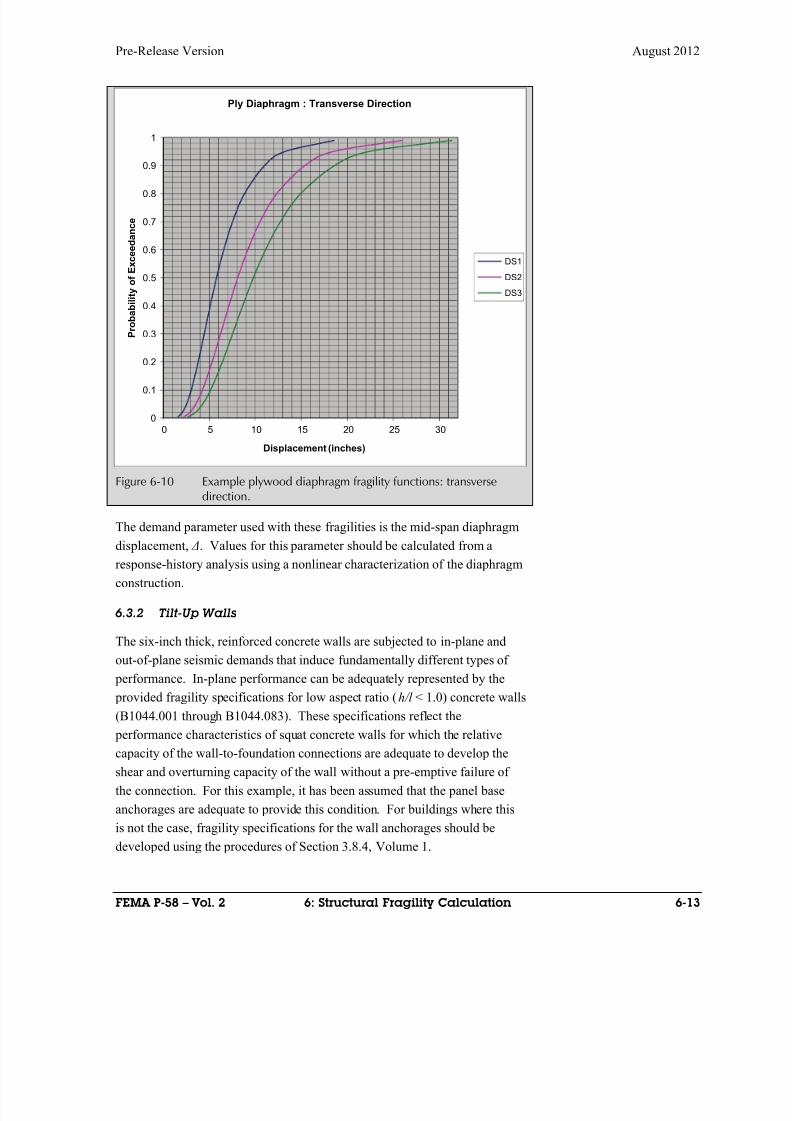
8/12/2019 Seismic Performance Assessment of Buildings
http://slidepdf.com/reader/full/seismic-performance-assessment-of-buildings 205/358
Pre-Release Version August 2012
FEMA P-58 – Vol. 2 6: Structural Fragility Calculation 6-13
Figure 6-10 Example plywood diaphragm fragility functions: transversedirection.
The demand parameter used with these fragilities is the mid-span diaphragm
displacement, Δ. Values for this parameter should be calculated from aresponse-history analysis using a nonlinear characterization of the diaphragm
construction.
6.3.2 Tilt-Up Walls
The six-inch thick, reinforced concrete walls are subjected to in-plane and
out-of-plane seismic demands that induce fundamentally different types of
performance. In-plane performance can be adequately represented by the
provided fragility specifications for low aspect ratio (h/l < 1.0) concrete walls
(B1044.001 through B1044.083). These specifications reflect the
performance characteristics of squat concrete walls for which the relativecapacity of the wall-to-foundation connections are adequate to develop the
shear and overturning capacity of the wall without a pre-emptive failure of
the connection. For this example, it has been assumed that the panel base
anchorages are adequate to provide this condition. For buildings where this
is not the case, fragility specifications for the wall anchorages should be
developed using the procedures of Section 3.8.4, Volume 1.
0
0.1
0.2
0.3
0.4
0.5
0.6
0.7
0.8
0.9
1
0 5 10 15 20 25 30
P r o b a b i l i t y o f E x c e e d a n c e
Displacement (inches)
Ply Diaphragm : Transverse Direction
DS1
DS2
DS3
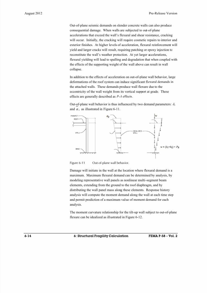
8/12/2019 Seismic Performance Assessment of Buildings
http://slidepdf.com/reader/full/seismic-performance-assessment-of-buildings 206/358
August 2012 Pre-Release Version
6-14 6: Structural Fragility Calculation FEMA P-58 – Vol. 2
Out-of-plane seismic demands on slender concrete walls can also produce
consequential damage. When walls are subjected to out-of-plane
accelerations that exceed the wall’s flexural and shear resistance, cracking
will occur. Initially, the cracking will require cosmetic repairs to interior and
exterior finishes. At higher levels of acceleration, flexural reinforcement will
yield and larger cracks will result, requiring patching or epoxy injection to
reconstitute the wall’s weather protection. At yet larger accelerations,
flexural yielding will lead to spalling and degradation that when coupled with
the effects of the supporting weight of the wall above can result in wall
collapse.
In addition to the effects of acceleration on out-of-plane wall behavior, large
deformations of the roof system can induce significant flexural demands in
the attached walls. These demands produce wall flexure due to the
eccentricity of the wall weight from its vertical support at grade. These
effects are generally described as P - Δ effects.
Out-of-plane wall behavior is thus influenced by two demand parameters: δr
and a r as illustrated in Figure 6-11.
Figure 6-11 Out-of-plane wall behavior.
Damage will initiate in the wall at the location where flexural demand is a
maximum. Maximum flexural demand can be determined by analysis, by
modeling representative wall panels as nonlinear multi-segment beam
elements, extending from the ground to the roof diaphragm, and by
distributing the wall panel mass along these elements. Response history
analysis will compute the moment demand along the wall at each time step
and permit prediction of a maximum value of moment demand for each
analysis.
The moment curvature relationship for the tilt-up wall subject to out-of-plane
flexure can be idealized as illustrated in Figure 6-12.

8/12/2019 Seismic Performance Assessment of Buildings
http://slidepdf.com/reader/full/seismic-performance-assessment-of-buildings 207/358
Pre-Release Version August 2012
FEMA P-58 – Vol. 2 6: Structural Fragility Calculation 6-15
M o m
e n t
Rotation
A
BC
D
Figure 6-12 Idealized moment-rotation relationship.
In order to construct fragility curves following the procedures of Section
3.8.4 of Volume 1, the median value of strength and dispersion have to be
calculated. The following example illustrates this calculation.
In order to fulfill Volume 1 Equation 3-1, the component design strength
needs to be calculated in accordance with an appropriate industry standard.
To accomplish this, the moment values associated with the control points of
the curve can be approximated as follows:
Step 1. Establish moment values associated with the control points A, B,
and C, in the moment-rotation relationship of Figure 6-12.
Point A: Cracking Moment
ACI 318-05 provides the following formula for cracking moment:
t
g r
cr y
I f M
where:
f r = modulus of rupture and for normal weight concrete can be taken as
'5.7 cr f f
I g = gross moment of inertia of section (neglecting reinforcing)
yt = distance from centroidal axis of section to tension face (neglectingreinforcing)
For the tilt-up wall section
3.47440005.7 r f psi
21612
)6(12 3
g I in4
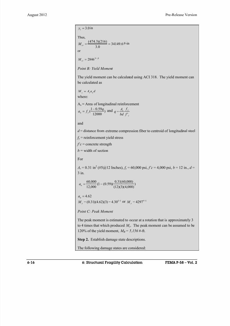
8/12/2019 Seismic Performance Assessment of Buildings
http://slidepdf.com/reader/full/seismic-performance-assessment-of-buildings 208/358
August 2012 Pre-Release Version
6-16 6: Structural Fragility Calculation FEMA P-58 – Vol. 2
0.3t y in
Thus,
6.341490.3
)216)(3.474(cr M #-in
or
ft
cr M #2846
Point B: Yield Moment
The yield moment can be calculated using ACI 318. The yield moment can
be calculated as
d a A M u s y
where:
As = Area of longitudinal reinforcement
)12000
59.01(
q f a yu
and
c
y s
f
f
bd
Aq
'
and
d = distance from extreme compression fiber to centroid of longitudinal steel
f y = reinforcement yield stress
f’c = concrete strength
b = width of section
For
A s = 0.31 in2 (#5@12 Inches), f y = 60,000 psi, f’c = 4,000 psi, b = 12 in., d =
3 in.
))000,4)(3)(12(
)000,60(31.0)(59.0(1(
000,12
000,60ua
62.4ua
130.4)3)(62.4)(31.0( k
y M or 1#4297 y M
Point C: Peak Moment
The peak moment is estimated to occur at a rotation that is approximately 3
to 4 times that which produced M y. The peak moment can be assumed to be
120% of the yield moment, M B = 5,156 #-ft.
Step 2. Establish damage state descriptions.
The following damage states are considered:
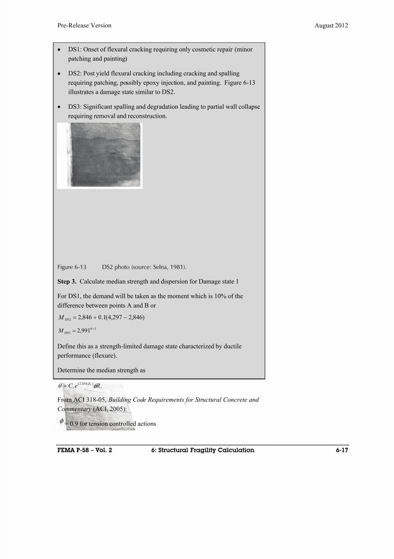
8/12/2019 Seismic Performance Assessment of Buildings
http://slidepdf.com/reader/full/seismic-performance-assessment-of-buildings 209/358
Pre-Release Version August 2012
FEMA P-58 – Vol. 2 6: Structural Fragility Calculation 6-17
DS1: Onset of flexural cracking requiring only cosmetic repair (minor
patching and painting)
DS2: Post yield flexural cracking including cracking and spalling
requiring patching, possibly epoxy injection, and painting. Figure 6-13
illustrates a damage state similar to DS2.
DS3: Significant spalling and degradation leading to partial wall collapse
requiring removal and reconstruction.
Figure 6-13 DS2 photo (source: Selna, 1981).
Step 3. Calculate median strength and dispersion for Damage state 1
For DS1, the demand will be taken as the moment which is 10% of the
difference between points A and B or
)846,2297,4(1.0846,21 DS M
1#
1991,2 DS M
Define this as a strength-limited damage state characterized by ductile
performance (flexure).
Determine the median strength as
nq ReC )054.2( 1
From ACI 318-05, Building Code Requirements for Structural Concrete and
Commentary (ACI, 2005):
= 0.9 for tension controlled actions

8/12/2019 Seismic Performance Assessment of Buildings
http://slidepdf.com/reader/full/seismic-performance-assessment-of-buildings 210/358

8/12/2019 Seismic Performance Assessment of Buildings
http://slidepdf.com/reader/full/seismic-performance-assessment-of-buildings 211/358
Pre-Release Version August 2012
FEMA P-58 – Vol. 2 6: Structural Fragility Calculation 6-19
The occurrence of DS 3 will be considered as a form of partial collapse and
will have a collapse fragility associated with it, based on incremental
dynamic analysis. This procedure is not illustrated here.
Table 6-4 summarizes the out-of-plane damage states and demand
parameters for the longitudinal tilt-up concrete walls. The walls are
subjected to out-of-plane acceleration and displacement effects that produce
a wall flexure behavior mechanism. Demands, in the form of peak bending
moment, are predicted by modeling individual wall panels as strings of
nonlinear beam elements with distributed mass, extending from the building
base to the roof diaphragm. Figure 6-14 presents a plot of the fragility
functions for damage states DS1 and DS2.
Table 6-4 Damage States – Tilt-Up walls Out-of-Plane Damage States
DamageState Damage Description Repair Description
BendingMoment
(#-ft)Dispersio
n
DS1 Onset of flexuralcracking requiringcosmetic repair
Over 4 foot distance at mid-height of wall groutpatch surface and repaint wall. Work occursover middle third of diaphragm span.
4,060 0.5
DS2 Post yield flexuralcracking with lightspalling, requiringpatching, possibleepoxy injection andpainting.
In addition to work done for DS1, over 6footdistance at mid-height of wall, patch spalls,epoxy inject 2 cracks (20 feet long each) andpaint wall. Work occurs over middle third ofdiaphragm span.
6,122 0.5
DS3 Significant spalling anddegradation leading topartial wall collapse.
Determined using incremental dynamic analysisand predicted by a building collapsefragility function.
- -

8/12/2019 Seismic Performance Assessment of Buildings
http://slidepdf.com/reader/full/seismic-performance-assessment-of-buildings 212/358
August 2012 Pre-Release Version
6-20 6: Structural Fragility Calculation FEMA P-58 – Vol. 2
Figure 6-14 Fragility functions for out-of-plane wall flexure.
6.3.3 Wall/Roof Attachments
As previously described, the wall and roof are attached to transfer in-plane
and out-of-plane wall and diaphragm demands. Separate attachments serve
to resist demands acting in the plane of the perimeter wall and out of the
plane of the perimeter wall. Consequential damage can occur to each type of
these attachments. Fragility functions which were derived analytically will
be developed for each of these attachments in the sections to follow.
6.3.3.1 In-Plane Attachment – Failure at Ledger Bolting
Figure 6-3 illustrates the in-plane wall attachment detail. Attachment
components include plywood nailing to the ledger and ledger bolting to the
concrete wall. Ledger nailing performance was previously addressed as part
of the fragility specification for the plywood diaphragm. The ledger bolting
system has four basic behavior modes that can result in damage. As
identified in National Design Specification (AF&PA, 2005) the four potential
limit states are:
0
0.1
0.2
0.3
0.4
0.5
0.6
0.7
0.8
0.9
1
0 10000 20000 30000
P r o b a b i l i t y o f D a m
a g e S t a t e O c c u r e n c e
Moment (#-ft)
DS
1
DS
2
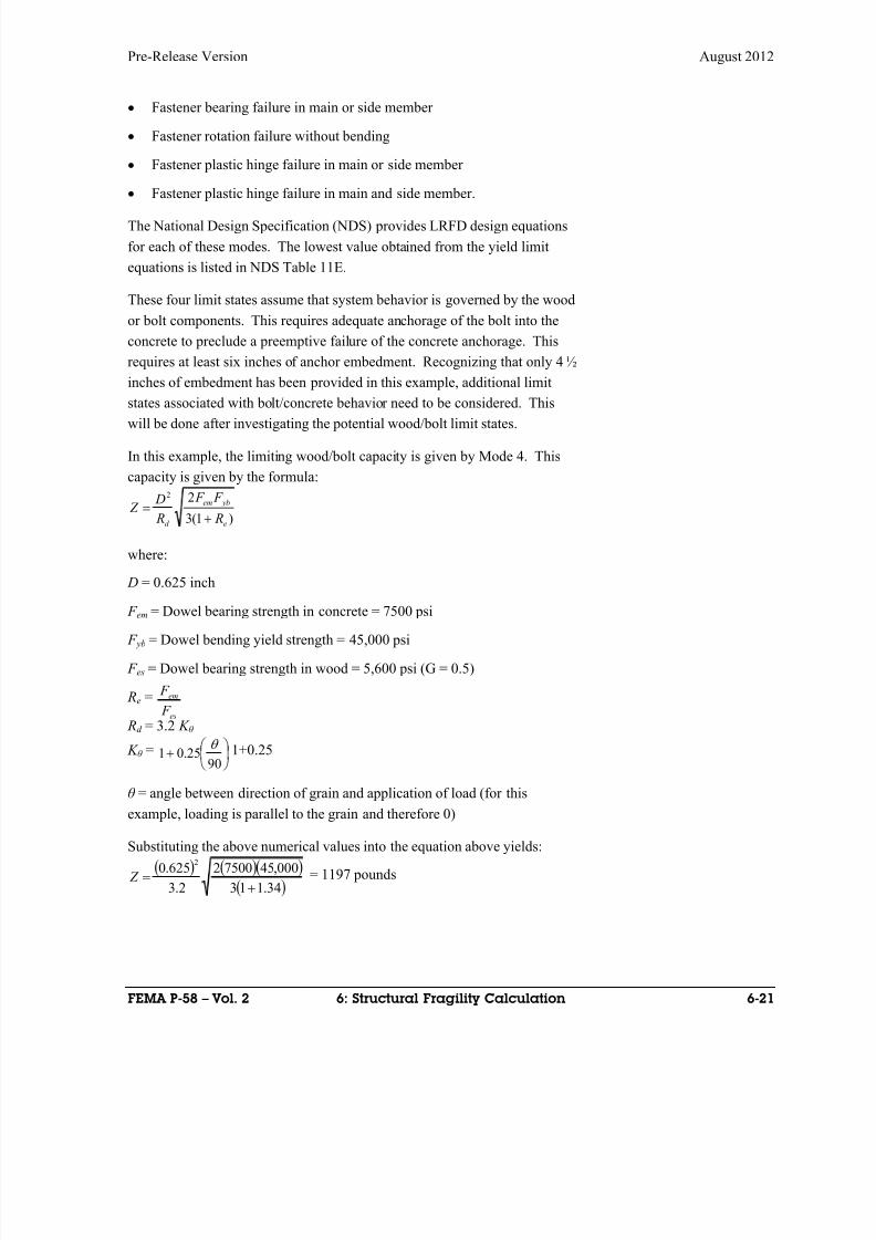
8/12/2019 Seismic Performance Assessment of Buildings
http://slidepdf.com/reader/full/seismic-performance-assessment-of-buildings 213/358
Pre-Release Version August 2012
FEMA P-58 – Vol. 2 6: Structural Fragility Calculation 6-21
Fastener bearing failure in main or side member
Fastener rotation failure without bending
Fastener plastic hinge failure in main or side member
Fastener plastic hinge failure in main and side member.
The National Design Specification (NDS) provides LRFD design equations
for each of these modes. The lowest value obtained from the yield limit
equations is listed in NDS Table 11E.
These four limit states assume that system behavior is governed by the wood
or bolt components. This requires adequate anchorage of the bolt into the
concrete to preclude a preemptive failure of the concrete anchorage. This
requires at least six inches of anchor embedment. Recognizing that only 4 ½
inches of embedment has been provided in this example, additional limit
states associated with bolt/concrete behavior need to be considered. Thiswill be done after investigating the potential wood/bolt limit states.
In this example, the limiting wood/bolt capacity is given by Mode 4. This
capacity is given by the formula:
)1(3
22
e
ybem
d R
F F
R
D Z
where:
D = 0.625 inch
F em = Dowel bearing strength in concrete = 7500 psi
F yb = Dowel bending yield strength = 45,000 psi
F es = Dowel bearing strength in wood = 5,600 psi (G = 0.5)
Re =
es
em
F
F
Rd = 3.2 K θ
K θ =
90
25.01 1+0.25
θ = angle between direction of grain and application of load (for this
example, loading is parallel to the grain and therefore 0)
Substituting the above numerical values into the equation above yields:
34.113
000,4575002
2.3
625.02
Z = 1197 pounds
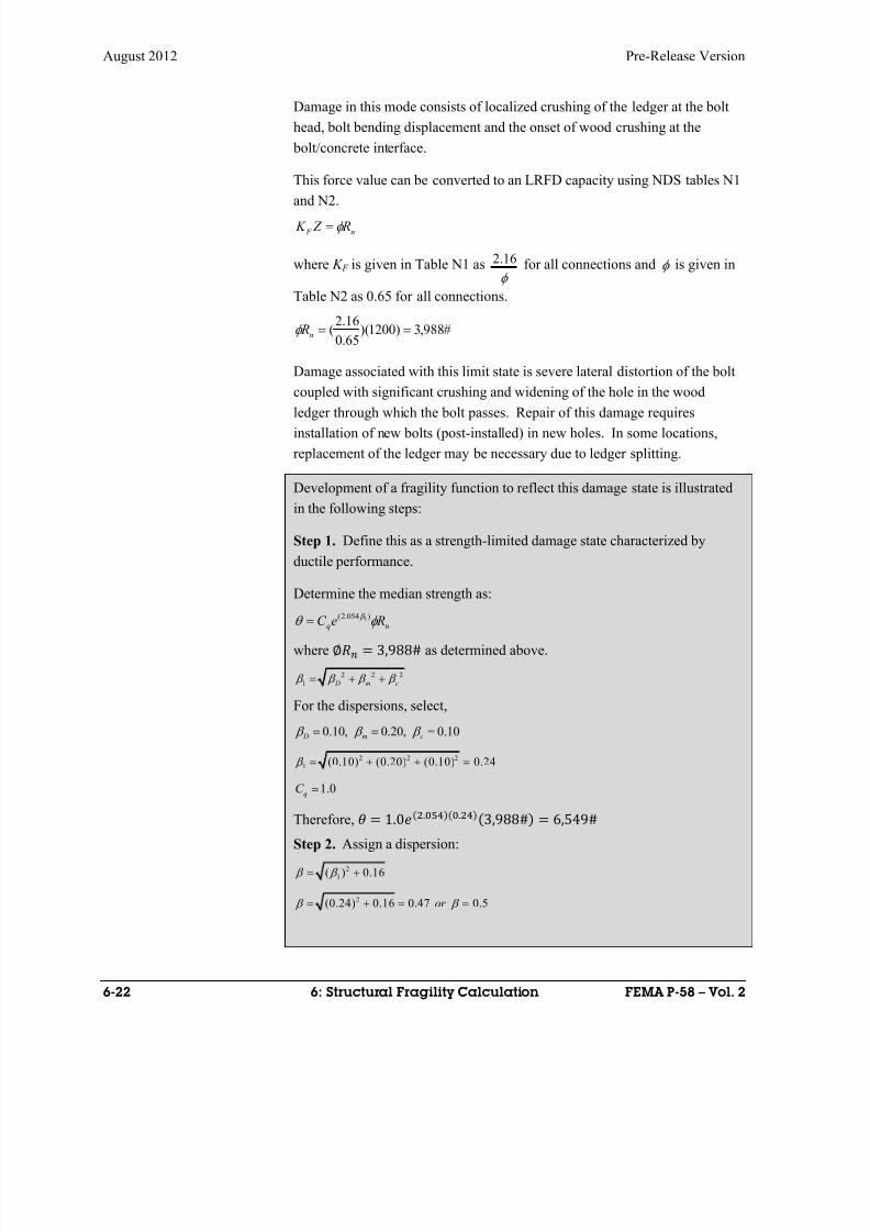
8/12/2019 Seismic Performance Assessment of Buildings
http://slidepdf.com/reader/full/seismic-performance-assessment-of-buildings 214/358
August 2012 Pre-Release Version
6-22 6: Structural Fragility Calculation FEMA P-58 – Vol. 2
Damage in this mode consists of localized crushing of the ledger at the bolt
head, bolt bending displacement and the onset of wood crushing at the
bolt/concrete interface.
This force value can be converted to an LRFD capacity using NDS tables N1
and N2.
n F R Z K
where K F is given in Table N1 as
16.2 for all connections and is given in
Table N2 as 0.65 for all connections.
#988,3)1200)(65.0
16.2( n R
Damage associated with this limit state is severe lateral distortion of the bolt
coupled with significant crushing and widening of the hole in the wood
ledger through which the bolt passes. Repair of this damage requires
installation of new bolts (post-installed) in new holes. In some locations,
replacement of the ledger may be necessary due to ledger splitting.
Development of a fragility function to reflect this damage state is illustrated
in the following steps:
Step 1. Define this as a strength-limited damage state characterized by
ductile performance.
Determine the median strength as:
nq ReC )054.2( 1
where ∅ 3,988# as determined above.
2 2 2
1 D m c
For the dispersions, select,
0.10, 0.20, 0.10 D m c
2 2 2
1 (0.10) (0.20) (0.10) 0.24
1.0qC
Therefore, 1.0..3,988# 6,549#
Step 2. Assign a dispersion:
2
1( ) 0.16
2(0.24) 0.16 0.47 0.5or
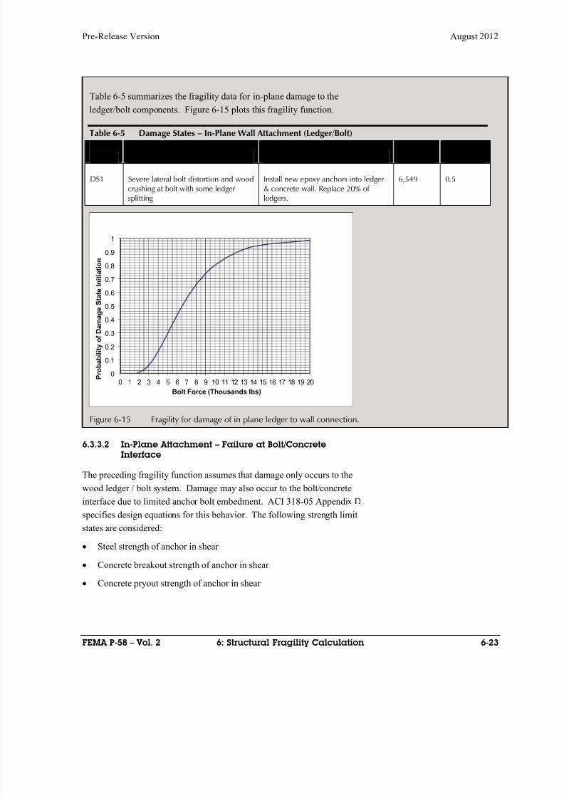
8/12/2019 Seismic Performance Assessment of Buildings
http://slidepdf.com/reader/full/seismic-performance-assessment-of-buildings 215/358
Pre-Release Version August 2012
FEMA P-58 – Vol. 2 6: Structural Fragility Calculation 6-23
6.3.3.2 In-Plane Attachment – Failure at Bolt/Concrete
Interface
The preceding fragility function assumes that damage only occurs to the
wood ledger / bolt system. Damage may also occur to the bolt/concrete
interface due to limited anchor bolt embedment. ACI 318-05 Appendix D
specifies design equations for this behavior. The following strength limit
states are considered:
Steel strength of anchor in shear
Concrete breakout strength of anchor in shear
Concrete pryout strength of anchor in shear
Table 6-5 summarizes the fragility data for in-plane damage to the
ledger/bolt components. Figure 6-15 plots this fragility function.
Table 6-5 Damage States – In-Plane Wall Attachment (Ledger/Bolt)
DamageState Damage Description Repair Description
Bolt Force(# lbs.) Dispersion
DS1 Severe lateral bolt distortion and woodcrushing at bolt with some ledgersplitting
Install new epoxy anchors into ledger& concrete wall. Replace 20% ofledgers.
6,549 0.5
Figure 6-15 Fragility for damage of in plane ledger to wall connection.
0
0.1
0.2
0.3
0.4
0.5
0.6
0.7
0.8
0.9
1
0 1 2 3 4 5 6 7 8 9 10 11 12 13 14 15 16 17 18 19 20 P r o b a b i l i t y o f D a m a g e S t a t e I n i t i a t i o n
Bolt Force (Thousands lbs)
8/12/2019 Seismic Performance Assessment of Buildings
http://slidepdf.com/reader/full/seismic-performance-assessment-of-buildings 216/358
August 2012 Pre-Release Version
6-24 6: Structural Fragility Calculation FEMA P-58 – Vol. 2
The median estimate of strength associated with each of these potential limit
states will be evaluated and the lowest value will be selected for fragility
function development.
Steel Strength of Anchor in Shear. For a cast-in-place headed stud anchor,
ACI 318-05 Appendix D provides the following capacity: uta se sa f nAV
Where n is the number of anchors in a group, n=1 for this example.
Ase is the effective cross section of the anchor and for a 5/8 inch diameter
stud anchor, Ase = 0.307 in2
f uta = tensile strength of anchor = 58 ksi.
lbsV sa 806,17)000,58)(307.0)(1(
Concrete Breakout Strength of Anchor in Shear. If it is assumed that
anchor bolts will be placed no closer than 12 inches from the edge of the tilt-
up panel, ACI 318-05 Appendix D provides the following capacity:
bvcved
vco
vccb V
A
AV )()(
where:
aaivc hC A ))(5.1)(2(
aiC edge distance = 12 inches
ah = wall thickness = 6 inches
vc A = (2)(1.5)(12)(6) = 216 in2
vco A = 4.5(C ai)2 = 4.5(12)2 = 648
ed = 1.0 for C a2 > 1.5 C a, C a2 = 24 + 5 = 29
cv = 1.4 for no cracking at service load levels
5.1'
0
2.0
0
))()(()(7 aicb C f d d
leV
where
le = heff = 4.5 -.31 = 4.2 inches
d0 = Anchor diameter = 0.625 inches
lbsV b 047,12)12)(000,4)(625.0()625.0
2.4(7
5.12.0
Therefore lbsV cb 622,5)047,12)(4.1)(0.1)(648
216(
Concrete Pryout Strength of Anchor in Shear. From ACI 318-05
Appendix D, the pryout capacity is:
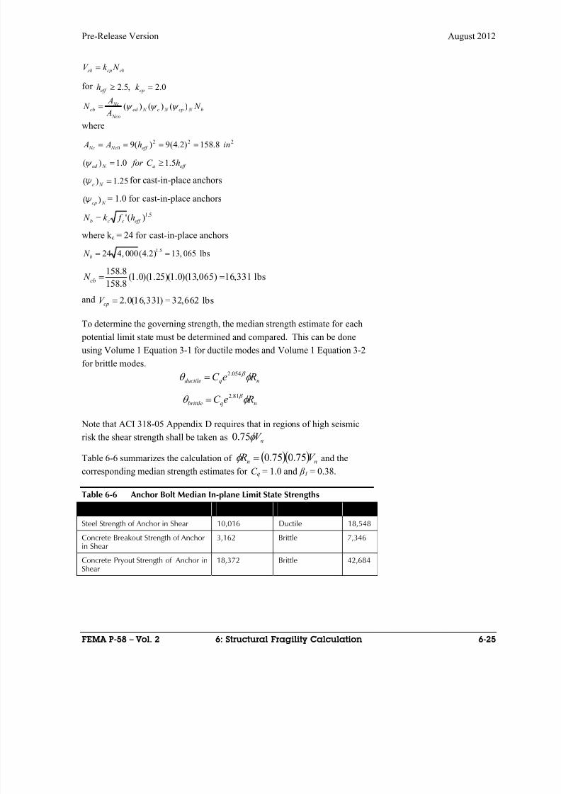
8/12/2019 Seismic Performance Assessment of Buildings
http://slidepdf.com/reader/full/seismic-performance-assessment-of-buildings 217/358
Pre-Release Version August 2012
FEMA P-58 – Vol. 2 6: Structural Fragility Calculation 6-25
cbcpcb N k V
for 0.2,5.2 cpeff k h
b N cp N c N ed
Nco
Nccb N
A
A N )()()(
where222
0 8.158)2.4(9)(9 inh A A eff Nc Nc
eff a N ed hC for 5.10.1)(
25.1)( N cfor cast-in-place anchors
N cp )( = 1.0 for cast-in-place anchors
5.1)(' eff ccb h f k N
where k c = 24 for cast-in-place anchors
1.524 4, 000(4.2) 13, 065 lbsb N
158.8(1.0)(1.25)(1.0)(13,065) 16,331 lbs
158.8cb N
and 2.0(16,331) 32,662 lbscpV
To determine the governing strength, the median strength estimate for each
potential limit state must be determined and compared. This can be done
using Volume 1 Equation 3-1 for ductile modes and Volume 1 Equation 3-2
for brittle modes.
nqductile ReC 054.2
nqbrittle ReC 81.2
Note that ACI 318-05 Appendix D requires that in regions of high seismic
risk the shear strength shall be taken as nV 75.0
Table 6-6 summarizes the calculation of nn V R 75.075.0 and the
corresponding median strength estimates for C q = 1.0 and β 1 = 0.38.
Table 6-6 Anchor Bolt Median In-plane Limit State Strengths
Limit State ΦR n (lbs) Failure Category θ (lbs)
Steel Strength of Anchor in Shear 10,016 Ductile 18,548
Concrete Breakout Strength of Anchorin Shear
3,162 Brittle 7,346
Concrete Pryout Strength of Anchor inShear
18,372 Brittle 42,684
8/12/2019 Seismic Performance Assessment of Buildings
http://slidepdf.com/reader/full/seismic-performance-assessment-of-buildings 218/358
8/12/2019 Seismic Performance Assessment of Buildings
http://slidepdf.com/reader/full/seismic-performance-assessment-of-buildings 219/358
Pre-Release Version August 2012
FEMA P-58 – Vol. 2 6: Structural Fragility Calculation 6-27
Bolt failure from concrete breakout
Using the example configuration, a capacity will be estimated for each of the
mechanisms outlined above. The mechanism that has the lowest median
capacity estimate will be used to develop a fragility function for the
assembly.
Diaphragm nailing. Diaphragm nailing consists of 10d nails at 3 inches
on center over an 8-foot length of purlin or subpurlins. The capacity can
be taken from AF&PA/ASCE 16, Table C4.2.2.D as 260 pounds per nail.
The total capacity is CDN = 260 #/nail x 4nails/foot x 8 feet = 8320
pounds = n R .
Device bolting at purlins or subpurlins. The bolting consists of 2 –
5/8” Фmachine bolts through the 4x12 purlin or 2 – 2x4 subpurlins, with
12 gage sideplates.
For the subpurlins (thickness – 3 inches), NDS Table 11G yields a Z 11
value of 2,270 lbs. For 2 bolts, the capacity is
lbslbsC DB 087,1565.0
16.2540,4 = n R
Device yield or fracture. The ASD capacity of the double holdown
device is given in the manufacturer’s catalog as 2 x 1,956 = 3,913 lbs.
Converting to an LRFD design strength yields:
lbslbsC Dd 002,1365.0
16.2913,3 = n R
Bolt yielding in tension. Using ACI 318, Appendix D, the bolt’s tensile
capacity can be estimated as:
lbsC DAB 747,14)2)(226)(.58()75.0( 2 = n R
Bolt failure from concrete breakout. Using ACI 318, Appendix D, the
design breakout strength can be estimated as follows:
bcp N c N ed N ec
NC
NC cb N
A
A N )()()()(
0
where 5.1)( ef ccb h f k N
and lbs N b 299,13)25.4(000,4245.1
24.302)5.20)(75.14( in A Nc
22
0 6.162)25.4(9 in A NC
0.1)( N ec (no eccentricity)
0.1)( N ed (Camin > 6.375)

8/12/2019 Seismic Performance Assessment of Buildings
http://slidepdf.com/reader/full/seismic-performance-assessment-of-buildings 220/358
August 2012 Pre-Release Version
6-28 6: Structural Fragility Calculation FEMA P-58 – Vol. 2
N c )( = 1.25 (cast-in-place)
cp = 1.0
therefore
lbs N cb
916,30)299,13)(0.1)(25.1)(0.1)(0.1(6.162
4.302
lbsC DBr 231,16)916,30)(75.0)(70.0( = n R
Table 6-7 summarizes the design strengths and estimated mediated strength
values for each of these limit states. For all failure modes, a C q value of 1.0
and β value of 0.24 has been used.
Table 6-7 Limit State Strengths Out-Of-Plane Attachment
Limit State ΦR n (lbs) Failure Category θ (lbs)
Diaphragm Nailing 8,320 lbs Ductile 13,621
Device Bolting Wood 15,087 lbs Ductile 24,700
Device Yielding 13,002 lbs Ductile 21,286
Anchor Bolt Yielding 14,747 lb Ductile 24,143
Anchor Bolt Concrete Breakout 16,231 lbs Brittle 31,859
The lowest median capacity estimate is associated with the diaphragm
nailing. This estimate is significantly lower then that for the other limit
states. This suggests that it is the most likely to occur. The damage that can
be anticipated from the occurrence of this damage state consists of splitting
of the purlin and subpurlin and tear through of the nails through the
diaphragm plywood. Replacement of the purlin, plywood and renailing is the
repair required to restore the original integrity.
Development of the fragility function for this limit state is as follows:
Step 1. Define this as a strength –limited damage state characterized by
ductile performance.
Determine the median strength as:
nq ReC )054.2( 1
where lbs Rn 320,8
222
1 )()()( cm D
For the dispersions, assign
10.0,20.0,10.0 cm D
24.0)10.0()20.0()10.0( 222
1
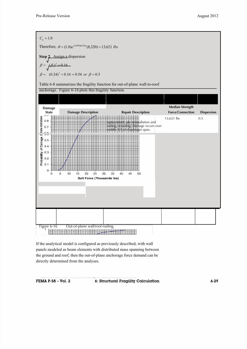
8/12/2019 Seismic Performance Assessment of Buildings
http://slidepdf.com/reader/full/seismic-performance-assessment-of-buildings 221/358
Pre-Release Version August 2012
FEMA P-58 – Vol. 2 6: Structural Fragility Calculation 6-29
If the analytical model is configured as previously described, with wall
panels modeled as beam elements with distributed mass spanning between
the ground and roof, then the out-of-plane anchorage force demand can be
directly determined from the analyses.
0.1qC
Therefore, lbse 621,13)320,8()0.1( )24.0)(054.2(
Step 2. Assign a dispersion
16.0)( 2
1
5.054.016.0)24.0( 2 or
Table 6-8 summarizes the fragility function for out-of-plane wall-to-roof
anchorage. Figure 6-16 plots this fragility function.
Table 6-8 Damage States – Out-of-Plane Wall Attachment (Purlin Nailing)
DamageState Damage Description Repair Description
Median Strength
Force/Connection Dispersion
DS1 Purlin/subpurlin splitting, nailtear out through ply, roofingtearing and distortion.
Shorings as needed, purlin, subpurlinreplacement, ply reinstallation andnailing, reroofing. Damage occurs overmiddle 1/3 of diaphragm span.
13,621 lbs 0.5
Figure 6-16 Out-of-plane wall/roof-nailing.
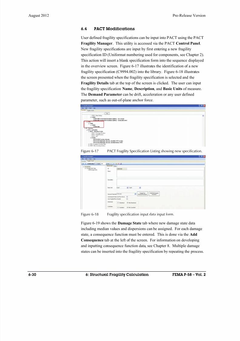
8/12/2019 Seismic Performance Assessment of Buildings
http://slidepdf.com/reader/full/seismic-performance-assessment-of-buildings 222/358
August 2012 Pre-Release Version
6-30 6: Structural Fragility Calculation FEMA P-58 – Vol. 2
6.4 PACT Modifications
User defined fragility specifications can be input into PACT using the PACT
Fragility Manager. This utility is accessed via the PACT Control Panel.
New fragility specifications are input by first entering a new fragility
specification ID (Uniformat numbering used for components, see Chapter 2).This action will insert a blank specification form into the sequence displayed
in the overview screen. Figure 6-17 illustrates the identification of a new
fragility specification (C9994.002) into the library. Figure 6-18 illustrates
the screen presented when the fragility specification is selected and the
Fragility Details tab at the top of the screen is clicked. The user can input
the fragility specification Name, Description, and Basic Units of measure.
The Demand Parameter can be drift, acceleration or any user defined
parameter, such as out-of-plane anchor force.
Figure 6-17 PACT Fragility Specification Listing showing new specification.
Figure 6-18 Fragility specification input data input form.
Figure 6-19 shows the Damage State tab where new damage state dataincluding median values and dispersions can be assigned. For each damage
state, a consequence function must be entered. This is done via the Add
Consequence tab at the left of the screen. For information on developing
and inputting consequence function data, see Chapter 8. Multiple damage
states can be inserted into the fragility specification by repeating the process.
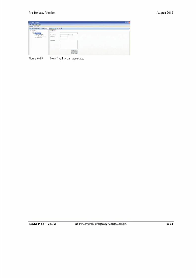
8/12/2019 Seismic Performance Assessment of Buildings
http://slidepdf.com/reader/full/seismic-performance-assessment-of-buildings 223/358
Pre-Release Version August 2012
FEMA P-58 – Vol. 2 6: Structural Fragility Calculation 6-31
Figure 6-19 New fragility damage state.

8/12/2019 Seismic Performance Assessment of Buildings
http://slidepdf.com/reader/full/seismic-performance-assessment-of-buildings 224/358
8/12/2019 Seismic Performance Assessment of Buildings
http://slidepdf.com/reader/full/seismic-performance-assessment-of-buildings 225/358
Pre-Release Version August 2012
FEMA P-58 – Vol. 2 7: Nonstructural Fragility Calculation 7-1
Chapter 7
Nonstructural FragilityCalculation
7.1 Introduction
Volume 1 Section 3.8.4 presents a general methodology for calculation of
fragility parameters for component damage states associated with limit states
that can be predicted by calculation. This chapter illustrates applications of
that methodology that can be used to estimate fragility parameters for
nonstructural components for damage states that can be predicted on the
basis of the following calculated structural limit states:
Strength-limited damage states when the occurrence of damage can be
predicted by a demand exceeding a calculable force capacity,
Ductility-limited damage states when the occurrence of damage can be
predicted by a demand exceeding a calculable amount of ductility,
Displacement-limited damage states when the occurrence of damage can
be predicted by a displacement demand exceeding a calculable value,
Code-based limit states when damage can be predicted as a function of a
code-specified demand parameter,
Overturning limit states when predicting overturning failure of
unanchored components, and
Sliding limit states when predicting sliding of unanchored components.
Note that this methodology is generally not applicable to damage states
associated with loss of electrical or mechanical function as these types of
failures cannot typically be predicted by structural calculation. Shake table
testing, or earthquake experience data are generally necessary to develop
fragility functions associated with loss of mechanical or electrical function,
unless the loss of functions can be directly tied to a structural limit state.
7.2 Unanchored Components
Unanchored components are vulnerable to damage associated with
overturning and sliding. Their vulnerability is dependent on the coefficient
of friction between the component and its resting surface (Table 7-1), the
amount of distance the component can slide before experiencing damage, and
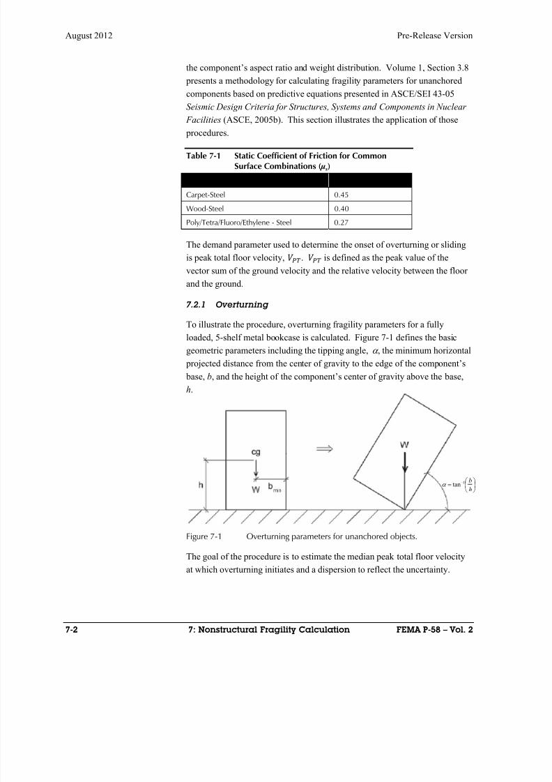
8/12/2019 Seismic Performance Assessment of Buildings
http://slidepdf.com/reader/full/seismic-performance-assessment-of-buildings 226/358
August 2012 Pre-Release Version
7-2 7: Nonstructural Fragility Calculation FEMA P-58 – Vol. 2
the component’s aspect ratio and weight distribution. Volume 1, Section 3.8
presents a methodology for calculating fragility parameters for unanchored
components based on predictive equations presented in ASCE/SEI 43-05
Seismic Design Criteria for Structures, Systems and Components in Nuclear
Facilities (ASCE, 2005b). This section illustrates the application of those
procedures.
Table 7-1 Static Coefficient of Friction for CommonSurface Combinations ( μ s)
Contact Surfaces μ s (mean estimate)
Carpet-Steel 0.45
Wood-Steel 0.40
Poly/Tetra/Fluoro/Ethylene - Steel 0.27
The demand parameter used to determine the onset of overturning or sliding
is peak total floor velocity, . is defined as the peak value of the
vector sum of the ground velocity and the relative velocity between the floor
and the ground.
7.2.1 Overturning
To illustrate the procedure, overturning fragility parameters for a fully
loaded, 5-shelf metal bookcase is calculated. Figure 7-1 defines the basic
geometric parameters including the tipping angle, , the minimum horizontal
projected distance from the center of gravity to the edge of the component’s
base, b, and the height of the component’s center of gravity above the base,
h.
Figure 7-1 Overturning parameters for unanchored objects.
The goal of the procedure is to estimate the median peak total floor velocity
at which overturning initiates and a dispersion to reflect the uncertainty.
h
b1tan
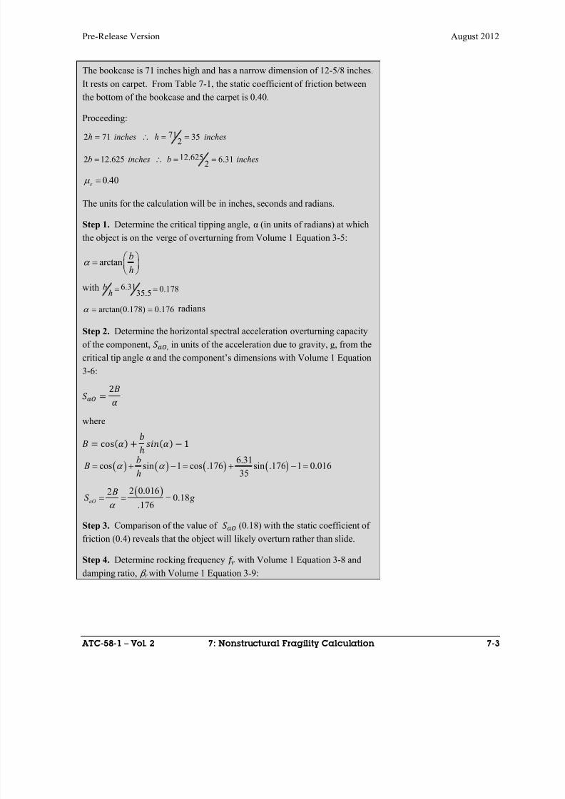
8/12/2019 Seismic Performance Assessment of Buildings
http://slidepdf.com/reader/full/seismic-performance-assessment-of-buildings 227/358
Pre-Release Version August 2012
ATC-58-1 – Vol. 2 7: Nonstructural Fragility Calculation 7-3
The bookcase is 71 inches high and has a narrow dimension of 12-5/8 inches.
It rests on carpet. From Table 7-1, the static coefficient of friction between
the bottom of the bookcase and the carpet is 0.40.
Proceeding:
incheshinchesh 352
71712
inchesbinchesb 31.62
625.12625.122
40.0 s
The units for the calculation will be in inches, seconds and radians.
Step 1. Determine the critical tipping angle, α (in units of radians) at which
the object is on the verge of overturning from Volume 1 Equation 3-5:
arctanb
h
with 6.31 0.17835.5
bh
176.0)178.0arctan( radians
Step 2. Determine the horizontal spectral acceleration overturning capacity
of the component, , in units of the acceleration due to gravity, g, from the
critical tip angle α and the component’s dimensions with Volume 1 Equation
3-6:
2
where
cos
1
6.31
cos sin 1 cos .176 sin .176 1 0.01635
b B
h
2 0.01620.18
.176aO
BS g
Step 3. Comparison of the value of (0.18) with the static coefficient of
friction (0.4) reveals that the object will likely overturn rather than slide.
Step 4. Determine rocking frequency with Volume 1 Equation 3-8 and
damping ratio, β r with Volume 1 Equation 3-9:
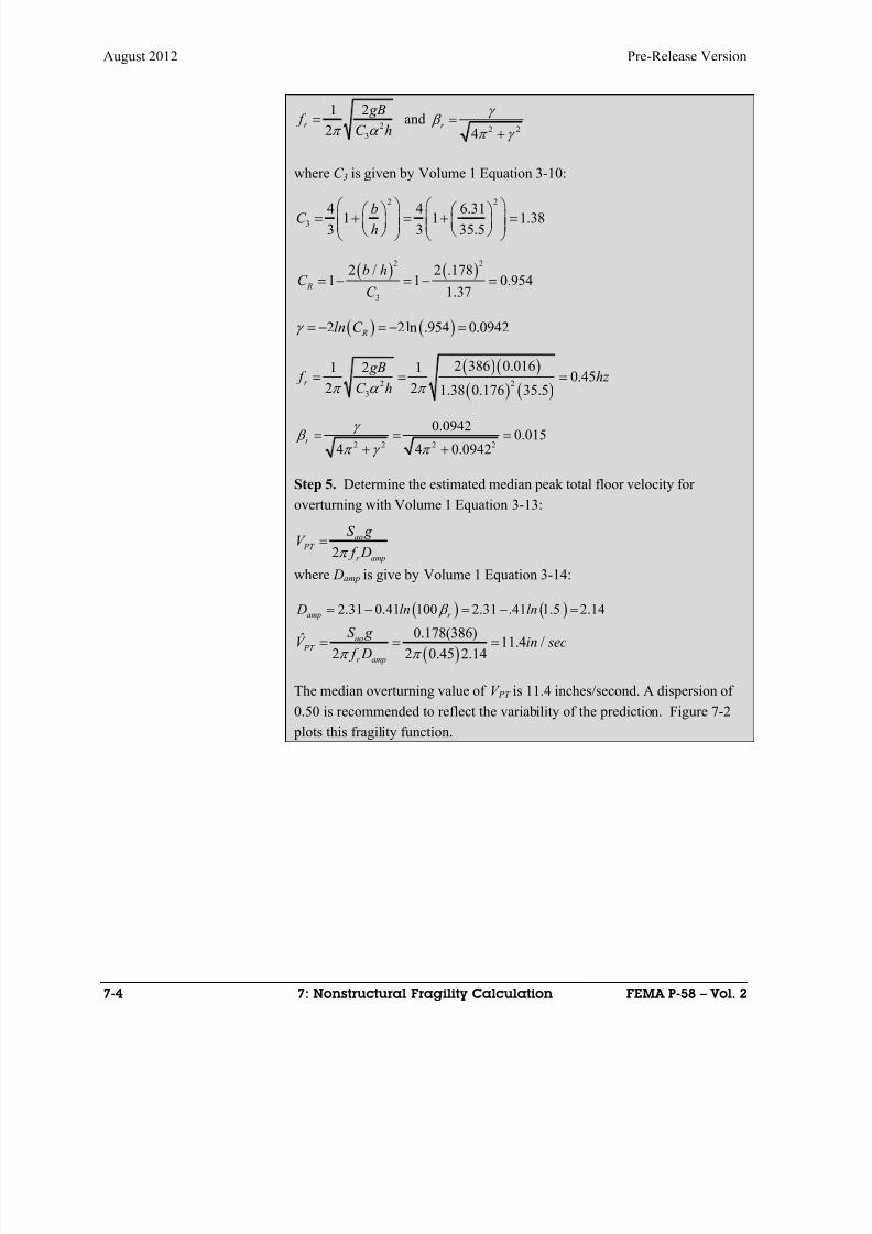
8/12/2019 Seismic Performance Assessment of Buildings
http://slidepdf.com/reader/full/seismic-performance-assessment-of-buildings 228/358
August 2012 Pre-Release Version
7-4 7: Nonstructural Fragility Calculation FEMA P-58 – Vol. 2
2
3
1 2
2r
gB f
C h and
2 24r
where C 3 is given by Volume 1 Equation 3-10:
2 2
3
4 4 6.311 1 1.38
3 3 35.5
bC
h
2 2
3
2 / 2 .178 1 1 0.954
1.37 R
b hC
C
2 2ln .954 0.0942 Rln C
22
3
2 386 0.0161 2 10.45
2 2 1.38 0.176 35.5r
gB f hz
C h
2 2 2 2
0.09420.015
4 4 0.0942r
Step 5. Determine the estimated median peak total floor velocity for
overturning with Volume 1 Equation 3-13:
2
ao PT
r amp
S g V
f D
where Damp is give by Volume 1 Equation 3-14:
2.31 0.41 100 2.31 .41 1.5 2.14amp r D ln ln
0.178(386)
11.4 /2 2 0.45 2.1
ˆ4
ao PT
r amp
S g V in sec
f D
The median overturning value of V PT is 11.4 inches/second. A dispersion of
0.50 is recommended to reflect the variability of the prediction. Figure 7-2
plots this fragility function.
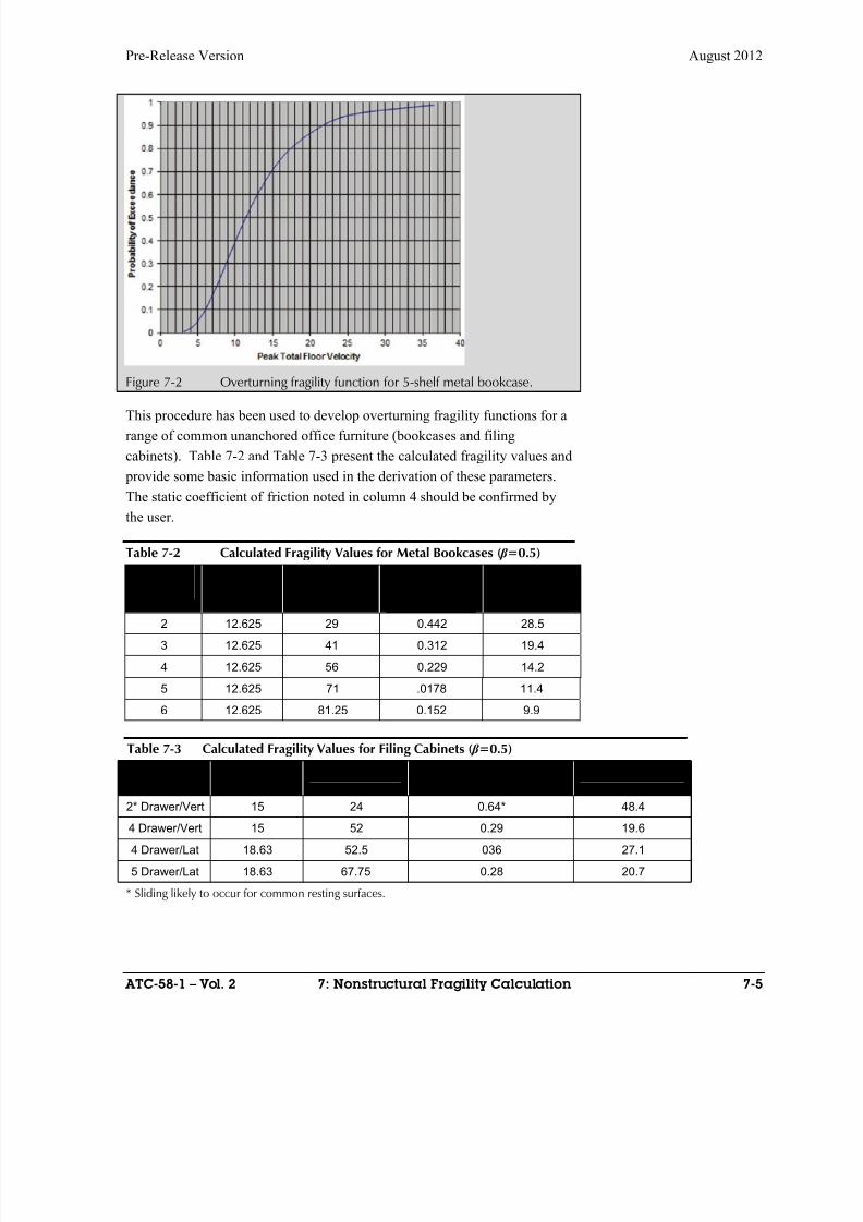
8/12/2019 Seismic Performance Assessment of Buildings
http://slidepdf.com/reader/full/seismic-performance-assessment-of-buildings 229/358
Pre-Release Version August 2012
ATC-58-1 – Vol. 2 7: Nonstructural Fragility Calculation 7-5
Figure 7-2 Overturning fragility function for 5-shelf metal bookcase.
This procedure has been used to develop overturning fragility functions for a
range of common unanchored office furniture (bookcases and filing
cabinets). Table 7-2 and Table 7-3 present the calculated fragility values and
provide some basic information used in the derivation of these parameters.
The static coefficient of friction noted in column 4 should be confirmed by
the user.
Table 7-2 Calculated Fragility Values for Metal Bookcases ( β =0.5)
Number ofShelves
DepthInchhes)
Height (Inches) μ s (minimumoverturning
before sliding)
(in/sec)
2 12.625 29 0.442 28.5
3 12.625 41 0.312 19.4
4 12.625 56 0.229 14.2
5 12.625 71 .0178 11.4
6 12.625 81.25 0.152 9.9
Table 7-3 Calculated Fragility Values for Filing Cabinets ( β =0.5)
Number ofDrawers/Type
Narrow PlanDim (Inches)
Height (Inches) μ s (minimum overturningbefore sliding)
(in/sec)
2* Drawer/Vert 15 24 0.64* 48.4
4 Drawer/Vert 15 52 0.29 19.6
4 Drawer/Lat 18.63 52.5 036 27.1
5 Drawer/Lat 18.63 67.75 0.28 20.7
* Sliding likely to occur for common resting surfaces.
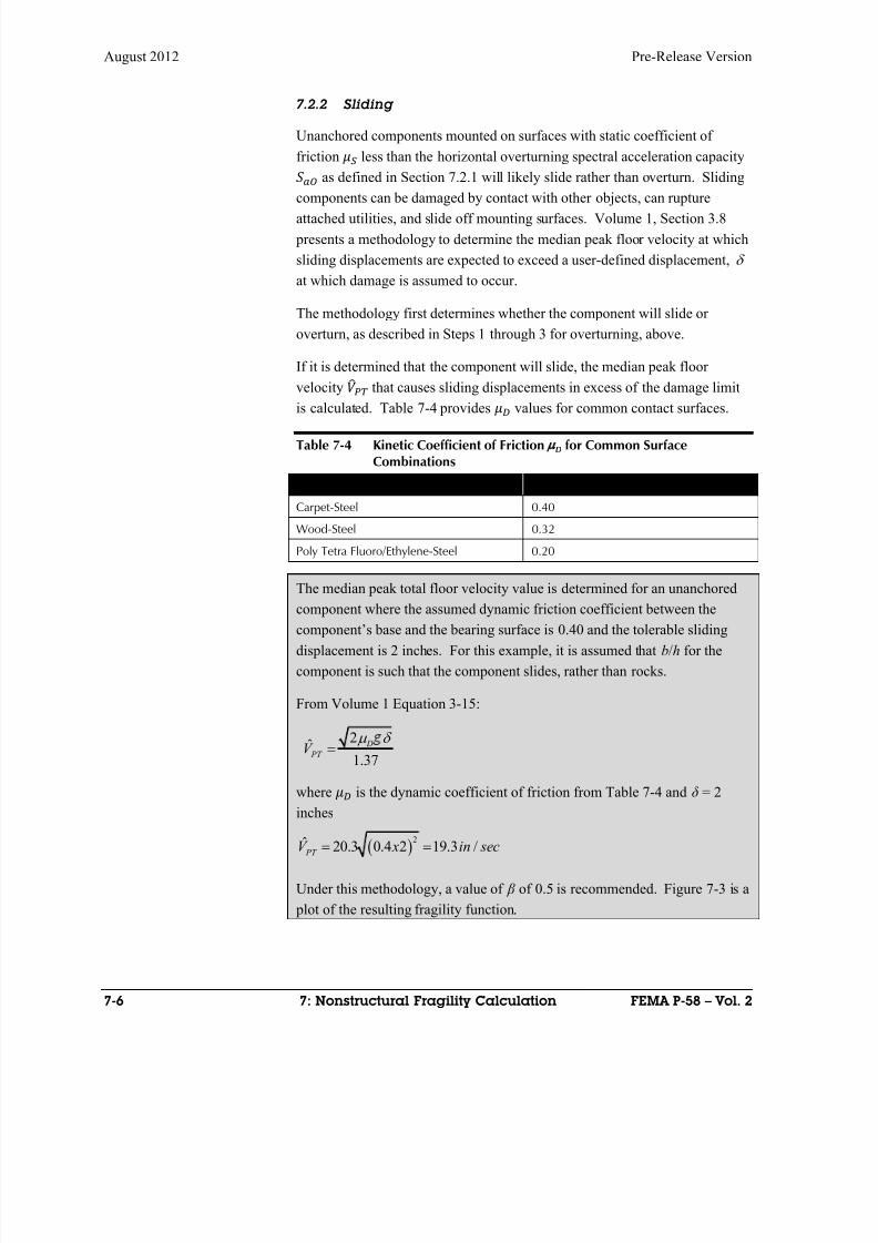
8/12/2019 Seismic Performance Assessment of Buildings
http://slidepdf.com/reader/full/seismic-performance-assessment-of-buildings 230/358
August 2012 Pre-Release Version
7-6 7: Nonstructural Fragility Calculation FEMA P-58 – Vol. 2
7.2.2 Sliding
Unanchored components mounted on surfaces with static coefficient of
friction less than the horizontal overturning spectral acceleration capacity
as defined in Section 7.2.1 will likely slide rather than overturn. Sliding
components can be damaged by contact with other objects, can ruptureattached utilities, and slide off mounting surfaces. Volume 1, Section 3.8
presents a methodology to determine the median peak floor velocity at which
sliding displacements are expected to exceed a user-defined displacement,
at which damage is assumed to occur.
The methodology first determines whether the component will slide or
overturn, as described in Steps 1 through 3 for overturning, above.
If it is determined that the component will slide, the median peak floor
velocity that causes sliding displacements in excess of the damage limit
is calculated. Table 7-4 provides values for common contact surfaces.
Table 7-4 Kinetic Coefficient of Friction D for Common SurfaceCombinations
Contact Surface D Mean Estimate
Carpet-Steel 0.40
Wood-Steel 0.32
Poly Tetra Fluoro/Ethylene-Steel 0.20
The median peak total floor velocity value is determined for an unanchored
component where the assumed dynamic friction coefficient between thecomponent’s base and the bearing surface is 0.40 and the tolerable sliding
displacement is 2 inches. For this example, it is assumed that b/h for the
component is such that the component slides, rather than rocks.
From Volume 1 Equation 3-15:
2
1.37ˆ D
PT V
where is the dynamic coefficient of friction from Table 7-4 and δ = 2
inches
2
20.3 0.4 2 19.3ˆ / PT
x iV n sec
Under this methodology, a value of β of 0.5 is recommended. Figure 7-3 is a
plot of the resulting fragility function.
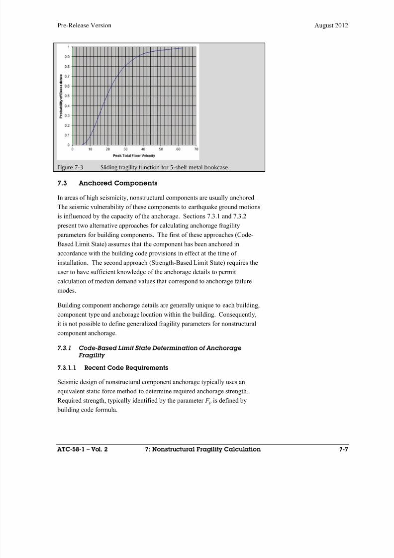
8/12/2019 Seismic Performance Assessment of Buildings
http://slidepdf.com/reader/full/seismic-performance-assessment-of-buildings 231/358
Pre-Release Version August 2012
ATC-58-1 – Vol. 2 7: Nonstructural Fragility Calculation 7-7
Figure 7-3 Sliding fragility function for 5-shelf metal bookcase.
7.3 Anchored Components
In areas of high seismicity, nonstructural components are usually anchored.
The seismic vulnerability of these components to earthquake ground motions
is influenced by the capacity of the anchorage. Sections 7.3.1 and 7.3.2
present two alternative approaches for calculating anchorage fragility
parameters for building components. The first of these approaches (Code-
Based Limit State) assumes that the component has been anchored in
accordance with the building code provisions in effect at the time of
installation. The second approach (Strength-Based Limit State) requires the
user to have sufficient knowledge of the anchorage details to permitcalculation of median demand values that correspond to anchorage failure
modes.
Building component anchorage details are generally unique to each building,
component type and anchorage location within the building. Consequently,
it is not possible to define generalized fragility parameters for nonstructural
component anchorage.
7.3.1 Code-Based Limit State Determination of Anchorage
Fragility
7.3.1.1 Recent Code Requirements
Seismic design of nonstructural component anchorage typically uses an
equivalent static force method to determine required anchorage strength.
Required strength, typically identified by the parameter F p is defined by
building code formula.
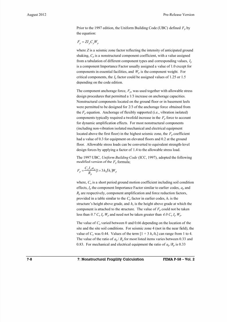
8/12/2019 Seismic Performance Assessment of Buildings
http://slidepdf.com/reader/full/seismic-performance-assessment-of-buildings 232/358
August 2012 Pre-Release Version
7-8 7: Nonstructural Fragility Calculation FEMA P-58 – Vol. 2
Prior to the 1997 edition, the Uniform Building Code (UBC) defined F p by
the equation:
p p p p F ZI C W
where Z is a seismic zone factor reflecting the intensity of anticipated ground
shaking, C p is a nonstructural component coefficient, with a value assigned
from a tabulation of different component types and corresponding values, I p
is a component Importance Factor usually assigned a value of 1.0 except for
components in essential facilities, and W p is the component weight. For
critical components, the I p factor could be assigned values of 1.25 or 1.5
depending on the code edition.
The component anchorage force, F p, was used together with allowable stress
design procedures that permitted a 1/3 increase on anchorage capacities.
Nonstructural components located on the ground floor or in basement leels
were permitted to be designed for 2/3 of the anchorage force obtained from
the F p equation. Anchorage of flexibly supported (i.e., vibration isolated)
components typically required a twofold increase in the F p force to account
for dynamic amplification effects. For most nonstructural components
(including non-vibration isolated mechanical and electrical equipment
located above the first floor) in the highest seismic zone, the F p coefficient
had a value of 0.3 for equipment on elevated floors and 0.2 at the ground
floor. Allowable stress loads can be converted to equivalent strength-level
design forces by applying a factor of 1.4 to the allowable stress load.
The 1997 UBC, Uniform Building Code (ICC, 1997), adopted the followingmodified version of the F p formula;
[1 3 ]a p p
p x r p p
C I a F h h W
R
where, C a is a short period ground motion coefficient including soil condition
effects, I p the component Importance Factor similar to earlier codes, a p and
R p are respectively, component amplification and force reduction factors,
provided in a table similar to the C p factor in earlier codes, hr is the
structure’s height above grade, and h x is the height above grade at which the
component is attached to the structure. The value of F p could not be taken
less than 0.7 C a I p W p and need not be taken greater than 4.0 C a I p W p.
The value of C a varied between 0 and 0.66 depending on the location of the
site and the site soil conditions. For seismic zone 4 (not in the near field), the
value of C a was 0.44. Values of the term [1 + 3 h x /hr ] can range from 1 to 4.
The value of the ratio of a p / R p for most listed items varies between 0.33 and
0.83. For mechanical and electrical equipment the ratio of a p / R p is 0.33

8/12/2019 Seismic Performance Assessment of Buildings
http://slidepdf.com/reader/full/seismic-performance-assessment-of-buildings 233/358
Pre-Release Version August 2012
ATC-58-1 – Vol. 2 7: Nonstructural Fragility Calculation 7-9
except for un-snubbed vibration isolated equipment for a p / R p had a value of
1.67. The potential range in anchorage design forces (in high seismic zones)
is quite large, varying from as low as 0.3g to as high as 1.76 g , depending on
component type and location within the structure.
For rigidly mounted mechanical and electrical equipment located on soil sitesin seismic zone 4, not in the near field and with I p = 1.0, the value of F p /W p
ranges from 0.308 at grade and lower floors to 0.58 at the roof level. Using
the same seismic zone and I p parameters, the value of F p/W p for vibration
isolated equipment ranges from 0.73 at grade to 1.76 at the roof. When
shallow anchors (anchors limited by concrete shear cone failure as opposed
to failure of the steel anchor) required anchor strengths were double these
values.
The 2000 through 2012 editions of the IBC, International Building Code
(ICC, 2000, 2009, 2012), as well as 2002 through 2010 editions ofASCE/SEI 7, Minimum Design Loads for Buildings and Other Structures
(ASCE, 2002, 2005a, 2010) specify the F p coefficient using the following
equation:
0.4[1 2 ]
p p DS p p
p
S I a F z h W
R
where S DS is a short period ground motion coefficient including site effects, z
is the height above grade at the point of component attachment to the
structure, h is height of the structure above grade, and other parameters are as
previously defined above. The value of F p cannot be taken less than0.3 S DS I p W p and need not be taken greater than 1.6 S DS I p W p. Forces
determined using this equation are considered to be strength-level.
The value of S DS varies between 0 and 2.5 depending on site location and
class. The value of the [1 + 2 z/h] term can vary from 1 to 3. The value of
the ratio of a p /R p for most listed items varies between 0.29 and 1.0. For most
rigidly mounted mechanical and electrical equipment, the a p / R p ratio ranges
between values of 0.4 and 1.25. For vibration isolation mounted equipment,
required anchor strength is increased by a factor of two, if the gap between
the lateral restraint and equipment exceeds ¼ inch. The potential range of
required anchorage strength (in high seismic zones) is quite large varying
from as low as 30% to as high as 176% of equipment weight.
Most nonstructural components can be treated as rigid boxes, and therefore
the equivalent static acceleration can be directly substituted for the peak floor
acceleration. This is the demand parameter specified in PACT for anchored
nonstructural components.

8/12/2019 Seismic Performance Assessment of Buildings
http://slidepdf.com/reader/full/seismic-performance-assessment-of-buildings 234/358
August 2012 Pre-Release Version
7-10 7: Nonstructural Fragility Calculation FEMA P-58 – Vol. 2
For vibration isolated equipment, peak floor acceleration can be amplified
significantly. In anchorage design, this effect is accounted for by the
specification of higher F p forces for use in design. To reflect this demand
amplification in the fragility calculation, it is recommended that the value of
θ be divided by 2.5 for isolated components to convert from spectral
acceleration to peak floor acceleration.
7.3.1.2 Procedure
Volume 1 Section 3.8.4 presents a code-based limit state procedure for the
case where there is insufficient information available to directly calculate the
anchorage capacity assuming that the original design met the requirements of
the applicable building code.
Peak floor acceleration is the demand parameter used to evaluate anchorage
failure. Where component anchorage was designed in accordance with a
building code that specifies strength-level, seismic forces (1997 UBC, or2000 or later edition of the International Building Code), the design
resistance, Rn, of an anchorage system, expressed as a peak floor
acceleration, can be taken as the ratio F p /W p, where F p and W p are as
described in the previous section. If anchorage was designed under codes
that specified design forces in an Allowable Stress Design format, the value
of Rn can be taken as 1.4 F p /W p.
Concrete anchorage is typically considered to have brittle failure modes
associated with breakout type failures. The median failure capacity of such
brittle nonstructural component anchorage designed to an equivalent staticacceleration coefficient F p /W p is given by Volume 1 Equation 3-2:
θ = C q e (2.81 β ) ( Rn)
where: C q = 0.5, and β = 0.5 and is the meadian peak floor acceleration for
anchorage failure.
Substituting, θ = 2.04 Rn
To obtain θ , the user must identify the building code under which component
installation was designed and determine the equivalent static acceleration
coefficient for the anchorage. This will require knowledge of the building
site ( Z, C a , S DS ), location within the building where the component is
supported (h x and hr ), and the appropriate I p, a p and R p coefficients.
The following examples illustrate application of this procedure, first for
rigidly mounted equipment, next for isolation-mounted equipment, and lastly
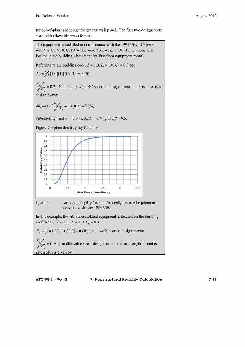
8/12/2019 Seismic Performance Assessment of Buildings
http://slidepdf.com/reader/full/seismic-performance-assessment-of-buildings 235/358
Pre-Release Version August 2012
ATC-58-1 – Vol. 2 7: Nonstructural Fragility Calculation 7-11
for out-of-plane anchorage for precast wall panel. The first two designs were
done with allowable stress forces.
The equipment is installed in conformance with the 1994 UBC, Uniform
Building Code (ICC, 1994), Seismic Zone 4, I p = 1.0. The equipment is
located in the building’s basement (or first floor equipment room)
Referring to the building code, Z = 1.0, I p = 1.0, C p = 0.3 and
2 1.0 1 0.3 0.23 p p p F W W
0.2 p
p
F
W . Since the 1994 UBC specified design forces in allowable stress
design format,
Rn 1.4 1.4 0.2 0.28 p
p
F g
W
Substituting, find θ = 2.04 x 0.28 = 0.49 g and β = 0.5.
Figure 7-4 plots this fragility function.
Figure 7-4 Anchorage fragility function for rigidly mounted equipmentdesigned under the 1994 UBC.
In this example, the vibration-isolated equipment is located on the building
roof. Again, Z = 1.0, I p = 1.0, C p = 0.3
2 1.0 1.0 0.3 0.6 p p F W in allowable stress design format.
0.60 p
p
F g
W in allowable stress design format and in strength format is
given Rn is given by:
8/12/2019 Seismic Performance Assessment of Buildings
http://slidepdf.com/reader/full/seismic-performance-assessment-of-buildings 236/358
August 2012 Pre-Release Version
7-12 7: Nonstructural Fragility Calculation FEMA P-58 – Vol. 2
Rn
1.4 1.4 0.60 0.84 p
p
F g g
W
Note however, that because this equipment is flexibly mounted, the value of
derived above should be divided by a factor of 2.5 to adjust for
amplification of peak floor acceleration. Thus:
0.842.04 0.682.5
g
Again, the dispersion is taken as β = 0.5. Figure 7-5 plots this fragility
function.
Figure 7-5 Anchorage fragility function for vibration isolated equipmentdesigned under the 1994 UBC.
Assume the precast wall panel was designed and installed in conformance
with ASCE/SEI 7-05. The wall panel is located between the roof and the
floor just below. From ASCE/SEI 7-05, find that S DS = 1.0, I p, a p = 1.0, R p =
1.25, z /h = 1.0
0.4 1.0 1.0 1.0 1 2 1.0
1.25
p
p
W F
0.96 p
p
F
W < max 1.6
p
p
F
W
Since ASCE/SEI 7-05 specifies design forces in a strength format, Rn isequal to W p /F p.
Rn
0.96 p
p
F
W
2.04 0.96 1.96 g with 5.0
8/12/2019 Seismic Performance Assessment of Buildings
http://slidepdf.com/reader/full/seismic-performance-assessment-of-buildings 237/358
Pre-Release Version August 2012
ATC-58-1 – Vol. 2 7: Nonstructural Fragility Calculation 7-13
7.3.2 Strength-Based Limit State Approach to Anchorage
Fragility Calculation
When details of a nonstructural component’s anchorage design are known,
the more detailed evaluation procedure of Volume 1, Section 3.8.4 can be
used to calculate the fragility parameters.
The strength capacity of an anchorage embedded in concrete is typically
determined using Appendix D of ACI 318-11, Building Code Requirements
for Structural Concrete and Commentary (ACI, 2011). This value can be
adjusted using the procedures of Section 3.8.4 to obtain the median capacity
associated with a failure mechanism (damage state). The median anchorage
capacity can be expressed in terms of a floor acceleration, which serves as
the fragility demand parameter.
This process requires the following steps:
Step 1. Determine the strength capacity of the anchorage detail for each
failure mode using the procedure of Section 3.8.4 and ACI 318-11, Appendix
D. Adjust the strength capacity to correspond to the median failure capacity.
Step 2. Determine the smallest median capacity of the anchorage using
Section 3.8.4.
Step 3. Determine the forces on each individual anchorage for a given
horizontal nonstructural component force F p using the connection geometry.
Step 4. Solve for F p that corresponds to the smallest anchorage median
failure capacity.
Step 5. Divide F p by the weight of the component, W p, to determine the
corresponding median floor acceleration. Assign a dispersion according to
Section 3.8.4.
The procedure is illustrated with an example below.
Assumptions:
A rigidly mounted equipment item is supported on a foundation pad at
the building’s first floor level. The equipment is tall and penetrates the first floor, where is it attached
for seismic and gravity forces.
The equipment’s center of gravity approximately aligns with the first
floor slab, such that the anchor bolts at the first floor are in shear only.
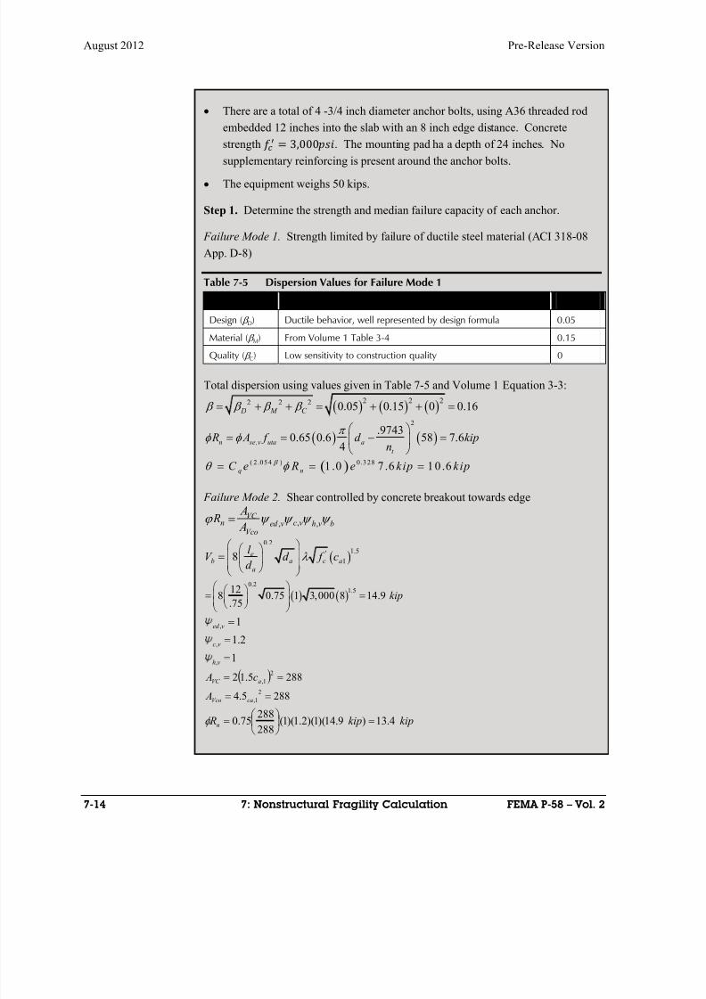
8/12/2019 Seismic Performance Assessment of Buildings
http://slidepdf.com/reader/full/seismic-performance-assessment-of-buildings 238/358
August 2012 Pre-Release Version
7-14 7: Nonstructural Fragility Calculation FEMA P-58 – Vol. 2
There are a total of 4 -3/4 inch diameter anchor bolts, using A36 threaded rod
embedded 12 inches into the slab with an 8 inch edge distance. Concrete
strength 3,000. The mounting pad ha a depth of 24 inches. No
supplementary reinforcing is present around the anchor bolts.
The equipment weighs 50 kips.
Step 1. Determine the strength and median failure capacity of each anchor.
Failure Mode 1. Strength limited by failure of ductile steel material (ACI 318-08
App. D-8)
Table 7-5 Dispersion Values for Failure Mode 1
Dispersion Discussion Value
Design ( D) Ductile behavior, well represented by design formula 0.05
Material ( M) From Volume 1 Table 3-4 0.15
Quality ( C) Low sensitivity to construction quality 0
Total dispersion using values given in Table 7-5 and Volume 1 Equation 3-3:
2 2 22 2 2 0.05 0.15 0 0.16 D M C
Failure Mode 2. Shear controlled by concrete breakout towards edge
,, ,VC
n c ved v h v bVco
A R
A
0.2
1.5'18 e
a c ab
a
l V d f c
d
0.2
1.5128 0.75 1 3,000 8 14.9
.75kip
1, ved
2.1, vc
1, vh
2885.122
1, aVC c A
2885.42
1, caVco A
kipkip Rn 4.13)9.14)(1)(2.1)(1(288
28875.0
2
,
.97430.65 0.6 58 7.6
4n se v uta a
t
R A f d kipn
( 2 .05 4 ) 0 .3 281 .0 7 .6 1 0 .6q nC e R e kip kip
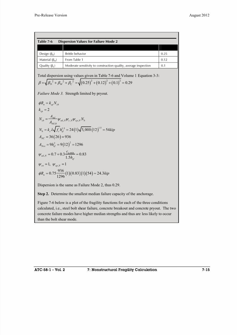
8/12/2019 Seismic Performance Assessment of Buildings
http://slidepdf.com/reader/full/seismic-performance-assessment-of-buildings 239/358
Pre-Release Version August 2012
ATC-58-1 – Vol. 2 7: Nonstructural Fragility Calculation 7-15
Table 7-6 Dispersion Values for Failure Mode 2
Dispersion Discussion Value
Design (D) Brittle behavior 0.25Material (M) From Table 1 0.12
Quality (C) Moderate sensitivity to construction quality, average inspection 0.1
Total dispersion using values given in Table 7-6 and Volume 1 Equation 3-3:
2 2 22 2 2 0.25 0.12 0.1 0.29 D M C
Failure Mode 3. Strength limited by pryout.
Dispersion is the same as Failure Mode 2, thus 0.29.
Step 2. Determine the smallest median failure capacity of the anchorage.
Figure 7-6 below is a plot of the fragility functions for each of the three conditions
calculated, i.e., steel bolt shear failure, concrete breakout and concrete pryout. The two
concrete failure modes have higher median strengths and thus are less likely to occur
than the bolt shear mode.
, , ,
1.5' 1.5
22
,min
,
,
2
24 1 3,000 12 54
36 26 936
9 9 12 1296
0.7 0.3 0.831.5
1, 1936
0.75 1 0.83 1 54 24.31296
n cp cb
cp
NC cb ed N c N cp N b
NCO
b c c ef
NC
Nco ef
a
ed N
ef
cn cp N
n
R k N
k
A N N
A
N k f h kip
A
A h
c
h
R kip

8/12/2019 Seismic Performance Assessment of Buildings
http://slidepdf.com/reader/full/seismic-performance-assessment-of-buildings 240/358
August 2012 Pre-Release Version
7-16 7: Nonstructural Fragility Calculation FEMA P-58 – Vol. 2
Figure 7-6 Fragility function for anchor bolt shear failure.
Based on the above, the governing median failure (shear) capacity of an individual
anchor is 10.6 kips.
Step 3. Determine the forces on an individual anchor. For the given component
configuration, the anchorage on an individual anchor is F p / 4.
Step 4. Solve for the F p that results in an anchorage force equal to the median
fragility anchorage failure force.
/ 4 10.6 , 42.4 p p F kip F kip
Step 5. Solve for the median failure acceleration
Median floor acceleration for anchorage failure:
/ 42.2 / 50 0.85 p p
F W g
Median peak floor acceleration for component anchorage = 0.85 g and β = 0.30.
7.4 Displacement-Based Limit State Approach to Define
Calculated Fragilities
Nonstructural components for which displacement based fragilities can bedeveloped include: exterior wall systems such as precast cladding designed
with slip joints of defined size and slide plate type seats for structural
members crossing expansion joints.
Exterior wall systems are generally constructed with a gap to accommodate
horizontal drift. Using geometric relationships, the size of the gap can be
expressed as a story drift ratio that the wall panel system can accommodate
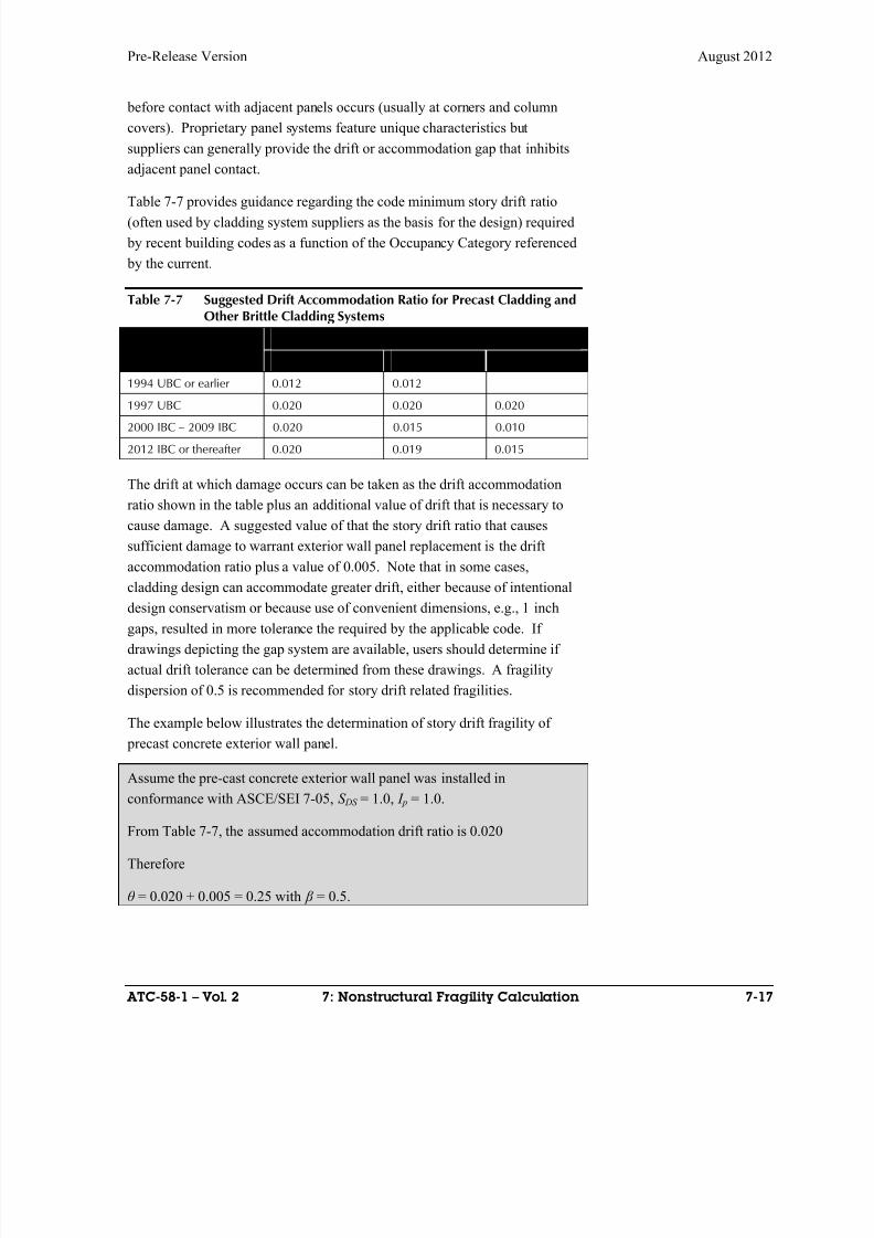
8/12/2019 Seismic Performance Assessment of Buildings
http://slidepdf.com/reader/full/seismic-performance-assessment-of-buildings 241/358
Pre-Release Version August 2012
ATC-58-1 – Vol. 2 7: Nonstructural Fragility Calculation 7-17
before contact with adjacent panels occurs (usually at corners and column
covers). Proprietary panel systems feature unique characteristics but
suppliers can generally provide the drift or accommodation gap that inhibits
adjacent panel contact.
Table 7-7 provides guidance regarding the code minimum story drift ratio(often used by cladding system suppliers as the basis for the design) required
by recent building codes as a function of the Occupancy Category referenced
by the current.
Table 7-7 Suggested Drift Accommodation Ratio for Precast Cladding andOther Brittle Cladding Systems
Building Code Building Occupancy Category according to ASCE/SEI 7)
II III IV
1994 UBC or earlier 0.012 0.012
1997 UBC 0.020 0.020 0.020
2000 IBC – 2009 IBC 0.020 0.015 0.010
2012 IBC or thereafter 0.020 0.019 0.015
The drift at which damage occurs can be taken as the drift accommodation
ratio shown in the table plus an additional value of drift that is necessary to
cause damage. A suggested value of that the story drift ratio that causes
sufficient damage to warrant exterior wall panel replacement is the drift
accommodation ratio plus a value of 0.005. Note that in some cases,
cladding design can accommodate greater drift, either because of intentional
design conservatism or because use of convenient dimensions, e.g., 1 inchgaps, resulted in more tolerance the required by the applicable code. If
drawings depicting the gap system are available, users should determine if
actual drift tolerance can be determined from these drawings. A fragility
dispersion of 0.5 is recommended for story drift related fragilities.
The example below illustrates the determination of story drift fragility of
precast concrete exterior wall panel.
Assume the pre-cast concrete exterior wall panel was installed in
conformance with ASCE/SEI 7-05, S DS = 1.0, I p = 1.0.
From Table 7-7, the assumed accommodation drift ratio is 0.020
Therefore
θ = 0.020 + 0.005 = 0.25 with β = 0.5.

8/12/2019 Seismic Performance Assessment of Buildings
http://slidepdf.com/reader/full/seismic-performance-assessment-of-buildings 242/358

8/12/2019 Seismic Performance Assessment of Buildings
http://slidepdf.com/reader/full/seismic-performance-assessment-of-buildings 243/358
Pre-Release Version August 2012
FEMA P-58 – Vol. 2 8: User-Defined Consequence Functions 8-1
Chapter 8
User-Defined ConsequenceFunctions
8.1 Introduction
Consequence functions are used to convert component and building damage
states into performance measures including: repair costs, repair times, unsafe
placarding probabilities, and casualties. As with each of the other
performance assessment steps, uncertainties arise in the translation of
damage states to consequences. Consequence functions reflect this
uncertainty in the form of probability distributions of consequences for each
damage state.
Each fragility specification includes a consequence function for each damage
state and each performance measure. Chapters 6 and 7 illustrate procedures
for development of fragility functions by calculation for those components
that do not have provided fragility specifications. Volume 1 describes other
procedures that can be used to develop component fragility functions using
laboratory test data, earthquake experience data, or expert judgment. This
chapter illustrates the consequence function development process. In
addition, it presents procedures that can be used to modify providedconsequence functions to reflect the unique circumstances users may
encounter in individual building assessments.
8.2 General Considerations
Repair cost and repair time consequence functions provided with PACT have
been developed by professional cost estimators using component damage
state repair descriptions. Repair descriptions were developed in
collaboration with engineering consultants familiar with component repair
techniques and cost estimators familiar with collateral cost and work. Repair
cost and repair time estimates were developed to include all collateral work,
such as finish removal and replacement, scaffolding, and debris removal,
associated with each component damage state repair. Consideration is given
to cost and time efficiencies that are gained by multiple component repairs
occurring in a given realization.

8/12/2019 Seismic Performance Assessment of Buildings
http://slidepdf.com/reader/full/seismic-performance-assessment-of-buildings 244/358
August 2012 Pre-Release Version
8-2 8: User-Defined Consequence Functions FEMA P-58 – Vol. 2
Values for the 10th 50th and 90th percentile levels were developed to capture
estimating uncertainty. To facilitate PACT programming, consequence
functions are structured to reflect either normal or lognormal probability
distributions. Median values and either the coefficient of variation or
dispersion were calculated from the cost data using a least squares fit
algorithm. The resulting consequence functions are included in the provided
fragility specifications.
When building collapse does not occur, some component damage states may
result in localized potential for casualties. For each damage state, a
determination is made as to whether deaths or serious injuries are possible as
a result of the damage. For damage states deemed to present a potential for
deaths or serious injuries, an “impacted area” is estimated. The impacted
area is that floor space adjacent to the damaged component in which there
would be risk of injury. For example, the impacted area for ceiling systems
is estimated as the floor area directly underneath the ceiling. For HVACducting, the area is estimated as 15 square feet per 5-foot duct length for
ducts with less than 6 square feet of cross-sectional area. The likelihood of
serious injuries or casualties in the impacted area is estimated based on the
component’s weight and location and judgment. For both ceiling systems
and HVAC ducting, the fatality rate is taken as zero. The serious injury rate
is taken as 10% for ceiling systems and 5% for HVAC ducting. A dispersion
of 0.5 is assigned for all fatality and serious injury estimates. The population
models are used to establish the number of persons likely to be present within
the impacted zone.
The likelihood of unsafe placard posting is determined using engineering
judgment. For most nonstructural components, an unsafe placard posting is
judged unlikely as a consequence of their damaged condition. A few notable
exceptions include sprinklers (since their failure affects the post-earthquake
fire life-safety of the building) and suspended ceiling systems (since their
failure can create the impression of significant damage that may cause a post-
earthquake inspector to post the building as unsafe). Most structural
components were judged to have the potential for an unsafe placard posting
since their damage can result in a reduction of the gravity or lateral-load
capacity of the building. For each component damage state, a ratio isestablished that reflects the number of damaged components out of the total
number of similar components at a given story or floor that would result in
an unsafe placard posting. For example, special concentrically-braced
frames with wide flange braces are assigned the following fractions by
damage state:
DS 1: Not applicable, unsafe placard posting not probable

8/12/2019 Seismic Performance Assessment of Buildings
http://slidepdf.com/reader/full/seismic-performance-assessment-of-buildings 245/358
Pre-Release Version August 2012
ATC-58-1 – Vol. 2 8: Development of User Defined Consequence Functions 8-3
DS 2: 60% of total quantity will result in unsafe placard posting
DS 3: 40% of total quantity will result in unsafe placard posting
DS 4: 20% of total quantity will result in unsafe placard posting
Generally, the fraction of the total quantity that will result in unsafe placarding reduces with the severity of the damage state given that it takes
fewer occurrences to cause post-earthquake inspector concern when such
damage is observed, and also reflecting that the effect on the building’s post-
earthquake resistance increases with the more severe damage states.
Consistent with casualty-related estimates, a dispersion of 0.5 is assigned for
all unsafe placard posting estimates.
Key considerations for developing consequence functions for the four
performance measures include:
Repair Cost and Repair Time. A detailed description of repair scope is
needed to enable estimation of repair labor and materials. The repair
description must include all work associated with repair of the actual damage
as well as collateral work associated with removal and replacement of
finishes, relocation of utilities, provision of scaffolding and similar actions.
Casualty and Unsafe Placard Posting. Judgment is required to assess if the
damage state is likely to result in fatalities, serious injuries or unsafe placard
posting. For casualties an impacted area and rate of severity must be defined
for casualty and serious injury. For unsafe placarding, consideration must be
given to the appearance of damage, and the effect it may have on post-
earthquake inspectors as well as the actual affect the damage will have on the
building’s post-earthquake safety. Predicted damage that significantly
increases the probability of building collapse in aftershocks should trigger
unsafe placarding, whether or not the damage is directly observable to post-
earthquake inspectors. Similarly, damage that could appear substantive to
post-earthquake inspectors should be assumed to be capable of triggering
unsafe placarding, even though the actual reduction in building safety may be
small.
8.3 Performance Measure Consequences
8.3.1 Repair Cost
The following steps outline the process for converting a component damage
state into a repair cost consequence.

8/12/2019 Seismic Performance Assessment of Buildings
http://slidepdf.com/reader/full/seismic-performance-assessment-of-buildings 246/358
August 2012 Pre-Release Version
8-4 8: User-Defined Consequence Functions FEMA P-58 – Vol. 2
8.3.1.1 Establish Required Repair Actions
Where multiple repair options exist, users must choose which strategy to use,
or alternatively, select multiple strategies and develop consequences for each.
In the latter case, the uncertainty of each method will be calculated by taking
a weighted-average value of the costs associated with each as the medianestimate of repair cost. Accordingly, in order to cover the range of potential
repair options and cost, disperions should be selected sufficiently large.
Typically, only one repair strategy will be selected, being the lowest-cost
acceptable solution.
8.3.1.2 Establish Repair Boundaries and Interfaces
A considerable amount of overlap and double-counting is possible in
estimating repair work on a component basis. For example, repair of a
structural element may require removal of architectural finishes and
mechanical/electrical system components that prevent access to the damagedstructure. However, the finishes and mechanical/electrical systems may be
directly damaged resulting in double-counting of the repair of these
components.
Generally, the repair scope should include all necessary access work,
including removal and replacement of finishes or mechanical/electrical work
and scaffolding or other staging. For more severe damage states, it may be
advisable to exclude removal and replacement of finishes or the
mechanical/electrical work associated with a structural repair, assuming that
as more severe damage occurs, these components will become damaged and
require repair by themselves. Users should consider the likelihood that these
systems will be directly damaged and if so, exclude them from the user
defined consequence function being developed.
Wall finishes other than paint should always be disregarded for User Defined
Consequence Functions since these components are identified separately in
the performance model.
8.3.1.3 Consider Associated Work Items
The following items should generally be included in damage repair
estimates:
Temporary relocation and protection of building contents
Removal and reinstallation of covering elements
Cutting in, patching and repairing of adjacent building elements
Clean-up

8/12/2019 Seismic Performance Assessment of Buildings
http://slidepdf.com/reader/full/seismic-performance-assessment-of-buildings 247/358
Pre-Release Version August 2012
ATC-58-1 – Vol. 2 8: Development of User Defined Consequence Functions 8-5
Staging and access
Costs should include subcontractor level mark-up, including overhead and
profit. General contractor mark-up should not be included since this is
separately addressed.
8.3.1.4 Estimate the Repair Cost
Using an appropriate estimating methodology, develop an estimate for the
repair cost. Since most repairs are not standard work found in cost
estimating guides, it is usually necessary to formulate an estimate using local
expertise and judgment regarding the labor hours and materials needed to
execute the specific work required. Allowances should be included for scope
not specifically identified.
8.3.1.5 Establish Cost Ranges
8.3.1.5.1 Establish Cost Distribution PACT is structured to use probabilistically defined cost ranges. Best
estimate, lower bound and upper bound costs should be identified and then a
lognormal or normal distribution should be fit to these bounds, based on the
User’s judgment.
8.3.1.5.2 Establish Quantity Ranges where Appropriate
The methodology is formulated to allow for cost adjustment based on
quantity of damage, recognizing that for many repairs there are economies of
scale. Users can enter lower and upper costs per unit of repair as well ascorresponding upper and lower bound quantities at which these costs apply.
Dispersions are assumed to be constant regardless of the quantity of repairs
that must be conducted.
As an example, consider that for a particular component and damage state, if
fewer than three of components are damaged in a realization, the unit repair
cost has a median value of $15,000 while if more than ten components
require repair in a realization, the unit median cost decreases to $8,000 per
item. The user can enter a lower bound of three, with an associated median
cost of $15,000, and an upper bound of 10, with an associated median cost of
$8,000. For quantities intermediate to the upper and lower bounds, PACT
applies linear interpolation.
8.3.2 Repair Time
The following steps outline the process for converting the occurrence of a
component damage state into a repair time consequence.
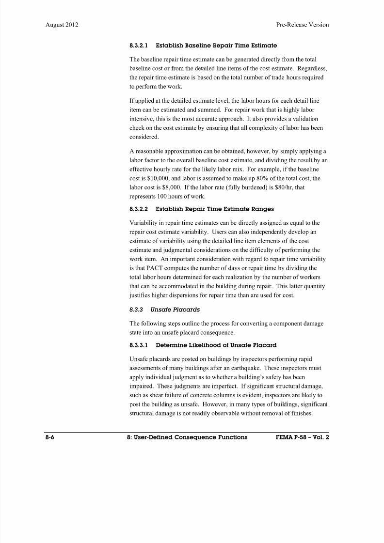
8/12/2019 Seismic Performance Assessment of Buildings
http://slidepdf.com/reader/full/seismic-performance-assessment-of-buildings 248/358
August 2012 Pre-Release Version
8-6 8: User-Defined Consequence Functions FEMA P-58 – Vol. 2
8.3.2.1 Establish Baseline Repair Time Estimate
The baseline repair time estimate can be generated directly from the total
baseline cost or from the detailed line items of the cost estimate. Regardless,
the repair time estimate is based on the total number of trade hours required
to perform the work.
If applied at the detailed estimate level, the labor hours for each detail line
item can be estimated and summed. For repair work that is highly labor
intensive, this is the most accurate approach. It also provides a validation
check on the cost estimate by ensuring that all complexity of labor has been
considered.
A reasonable approximation can be obtained, however, by simply applying a
labor factor to the overall baseline cost estimate, and dividing the result by an
effective hourly rate for the likely labor mix. For example, if the baseline
cost is $10,000, and labor is assumed to make up 80% of the total cost, thelabor cost is $8,000. If the labor rate (fully burdened) is $80/hr, that
represents 100 hours of work.
8.3.2.2 Establish Repair Time Estimate Ranges
Variability in repair time estimates can be directly assigned as equal to the
repair cost estimate variability. Users can also independently develop an
estimate of variability using the detailed line item elements of the cost
estimate and judgmental considerations on the difficulty of performing the
work item. An important consideration with regard to repair time variability
is that PACT computes the number of days or repair time by dividing thetotal labor hours determined for each realization by the number of workers
that can be accommodated in the building during repair. This latter quantity
justifies higher dispersions for repair time than are used for cost.
8.3.3 Unsafe Placards
The following steps outline the process for converting a component damage
state into an unsafe placard consequence.
8.3.3.1 Determine Likelihood of Unsafe Placard
Unsafe placards are posted on buildings by inspectors performing rapid
assessments of many buildings after an earthquake. These inspectors must
apply individual judgment as to whether a building’s safety has been
impaired. These judgments are imperfect. If significant structural damage,
such as shear failure of concrete columns is evident, inspectors are likely to
post the building as unsafe. However, in many types of buildings, significant
structural damage is not readily observable without removal of finishes.
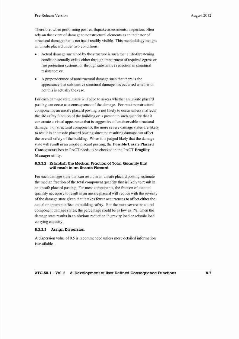
8/12/2019 Seismic Performance Assessment of Buildings
http://slidepdf.com/reader/full/seismic-performance-assessment-of-buildings 249/358
Pre-Release Version August 2012
ATC-58-1 – Vol. 2 8: Development of User Defined Consequence Functions 8-7
Therefore, when performing post-earthquake assessments, inspectors often
rely on the extent of damage to nonstructural elements as an indicator of
structural damage that is not itself readily visible. This methodology assigns
an unsafe placard under two conditions:
Actual damage sustained by the structure is such that a life-threateningcondition actually exists either through impairment of required egress or
fire protection systems, or through substantive reduction in structural
resistance; or,
A preponderance of nonstructural damage such that there is the
appearance that substantive structural damage has occurred whether or
not this is actually the case.
For each damage state, users will need to assess whether an unsafe placard
posting can occur as a consequence of the damage. For most nonstructural
components, an unsafe placard posting is not likely to occur unless it affectsthe life safety function of the building or is present in such quantity that it
can create a visual appearance that is suggestive of unobservable structural
damage. For structural components, the more severe damage states are likely
to result in an unsafe placard posting since the resulting damage can affect
the overall safety of the building. When it is judged likely that the damage
state will result in an unsafe placard posting, the Possible Unsafe Placard
Consequence box in PACT needs to be checked in the PACT Fragility
Manager utility.
8.3.3.2 Establish the Median Fraction of Total Quantity that
will result in an Unsafe Placard
For each damage state that can result in an unsafe placard posting, estimate
the median fraction of the total component quantity that is likely to result in
an unsafe placard posting. For most components, the fraction of the total
quantity necessary to result in an unsafe placard will reduce with the severity
of the damage state given that it takes fewer occurrences to affect either the
actual or apparent effect on building safety. For the most severe structural
component damage states, the percentage could be as low as 1%, when the
damage state results in an obvious reduction in gravity load or seismic load
carrying capacity.
8.3.3.3 Assign Dispersion
A dispersion value of 0.5 is recommended unless more detailed information
is available.
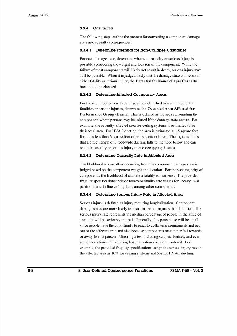
8/12/2019 Seismic Performance Assessment of Buildings
http://slidepdf.com/reader/full/seismic-performance-assessment-of-buildings 250/358
August 2012 Pre-Release Version
8-8 8: User-Defined Consequence Functions FEMA P-58 – Vol. 2
8.3.4 Casualties
The following steps outline the process for converting a component damage
state into casualty consequences.
8.3.4.1 Determine Potential for Non-Collapse Casualties
For each damage state, determine whether a casualty or serious injury is
possible considering the weight and location of the component. While the
failure of most components will likely not result in death, serious injury may
still be possible. When it is judged likely that the damage state will result in
either fatality or serious injury, the Potential for Non-Collapse Casualty
box should be checked.
8.3.4.2 Determine Affected Occupancy Areas
For those components with damage states identified to result in potential
fatalities or serious injuries, determine the Occupied Area Affected forPerformance Group element. This is defined as the area surrounding the
component, where persons may be injured if the damage state occurs. For
example, the casualty-affected area for ceiling systems is estimated to be
their total area. For HVAC ducting, the area is estimated as 15 square feet
for ducts less than 6 square foot of cross-sectional area. The logic assumes
that a 5 feet length of 3 foot-wide ducting falls to the floor below and can
result in casualty or serious injury to one occupying the area.
8.3.4.3 Determine Casualty Rate in Affected Area
The likelihood of casualties occurring from the component damage state is judged based on the component weight and location. For the vast majority of
components, the likelihood of causing a fatality is near zero. The provided
fragility specifications include non-zero fatality rate values for “heavy” wall
partitions and in-line ceiling fans, among other components.
8.3.4.4 Determine Serious Injury Rate in Affected Area
Serious injury is defined as injury requiring hospitalization. Component
damage states are more likely to result in serious injuries than fatalities. The
serious injury rate represents the median percentage of people in the affected
area that will be seriously injured. Generally, this percentage will be smallsince people have the opportunity to react to collapsing components and get
out of the affected area and also because components may either fall towards
or away from a person. Minor injuries, including scrapes, bruises, and even
some lacerations not requiring hospitalization are not considered. For
example, the provided fragility specifications assign the serious injury rate in
the affected area as 10% for ceiling systems and 5% for HVAC ducting.
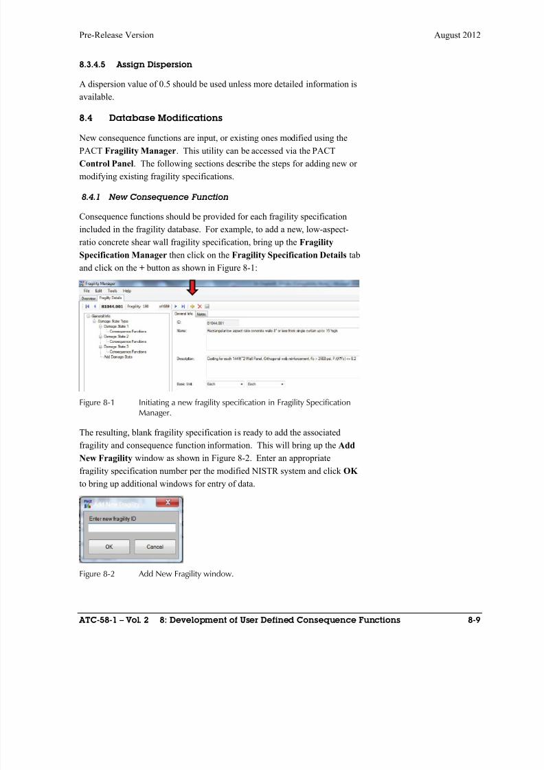
8/12/2019 Seismic Performance Assessment of Buildings
http://slidepdf.com/reader/full/seismic-performance-assessment-of-buildings 251/358
Pre-Release Version August 2012
ATC-58-1 – Vol. 2 8: Development of User Defined Consequence Functions 8-9
8.3.4.5 Assign Dispersion
A dispersion value of 0.5 should be used unless more detailed information is
available.
8.4 Database Modifications
New consequence functions are input, or existing ones modified using the
PACT Fragility Manager. This utility can be accessed via the PACT
Control Panel. The following sections describe the steps for adding new or
modifying existing fragility specifications.
8.4.1 New Consequence Function
Consequence functions should be provided for each fragility specification
included in the fragility database. For example, to add a new, low-aspect-
ratio concrete shear wall fragility specification, bring up the Fragility
Specification Manager then click on the Fragility Specification Details tab
and click on the + button as shown in Figure 8-1:
Figure 8-1 Initiating a new fragility specification in Fragility SpecificationManager.
The resulting, blank fragility specification is ready to add the associated
fragility and consequence function information. This will bring up the Add
New Fragility window as shown in Figure 8-2. Enter an appropriate
fragility specification number per the modified NISTR system and click OK
to bring up additional windows for entry of data.
Figure 8-2 Add New Fragility window.
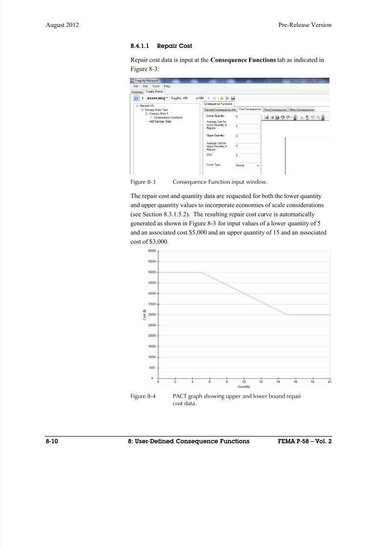
8/12/2019 Seismic Performance Assessment of Buildings
http://slidepdf.com/reader/full/seismic-performance-assessment-of-buildings 252/358
August 2012 Pre-Release Version
8-10 8: User-Defined Consequence Functions FEMA P-58 – Vol. 2
8.4.1.1 Repair Cost
Repair cost data is input at the Consequence Functions tab as indicated in
Figure 8-3:
Figure 8-3 Consequence Function input window.
The repair cost and quantity data are requested for both the lower quantity
and upper quantity values to incorporate economies of scale considerations
(see Section 8.3.1.5.2). The resulting repair cost curve is automatically
generated as shown in Figure 8-3 for input values of a lower quantity of 5
and an associated cost $5,000 and an upper quantity of 15 and an associated
cost of $3,000.
Figure 8-4 PACT graph showing upper and lower bound repaircost data.
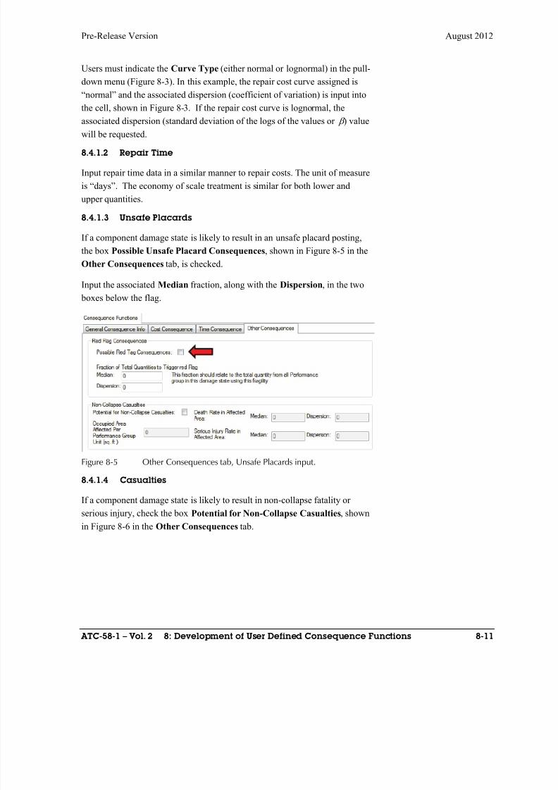
8/12/2019 Seismic Performance Assessment of Buildings
http://slidepdf.com/reader/full/seismic-performance-assessment-of-buildings 253/358
Pre-Release Version August 2012
ATC-58-1 – Vol. 2 8: Development of User Defined Consequence Functions 8-11
Users must indicate the Curve Type (either normal or lognormal) in the pull-
down menu (Figure 8-3). In this example, the repair cost curve assigned is
“normal” and the associated dispersion (coefficient of variation) is input into
the cell, shown in Figure 8-3. If the repair cost curve is lognormal, the
associated dispersion (standard deviation of the logs of the values or ) value
will be requested.
8.4.1.2 Repair Time
Input repair time data in a similar manner to repair costs. The unit of measure
is “days”. The economy of scale treatment is similar for both lower and
upper quantities.
8.4.1.3 Unsafe Placards
If a component damage state is likely to result in an unsafe placard posting,
the box Possible Unsafe Placard Consequences, shown in Figure 8-5 in the
Other Consequences tab, is checked.
Input the associated Median fraction, along with the Dispersion, in the two
boxes below the flag.
Figure 8-5 Other Consequences tab, Unsafe Placards input.
8.4.1.4 Casualties
If a component damage state is likely to result in non-collapse fatality or
serious injury, check the boxPotential for Non-Collapse Casualties
, shown
in Figure 8-6 in the Other Consequences tab.
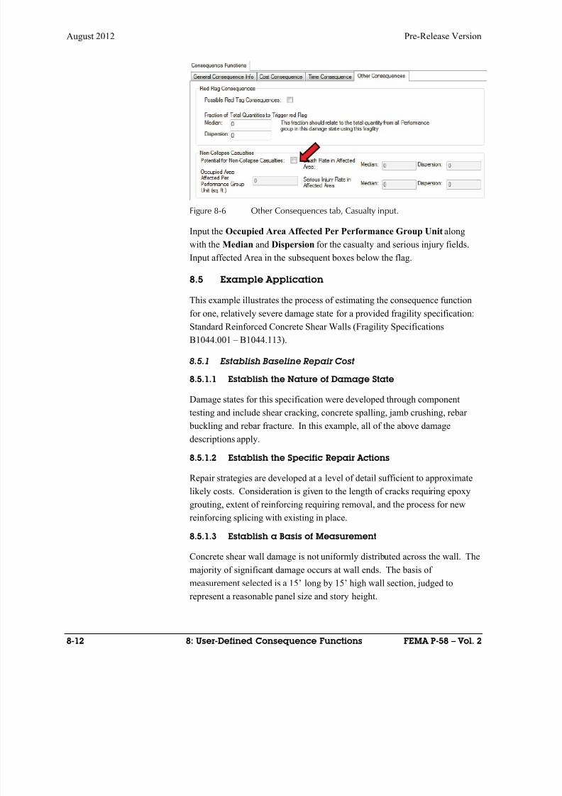
8/12/2019 Seismic Performance Assessment of Buildings
http://slidepdf.com/reader/full/seismic-performance-assessment-of-buildings 254/358
August 2012 Pre-Release Version
8-12 8: User-Defined Consequence Functions FEMA P-58 – Vol. 2
Figure 8-6 Other Consequences tab, Casualty input.
Input the Occupied Area Affected Per Performance Group Unit along
with the Median and Dispersion for the casualty and serious injury fields.
Input affected Area in the subsequent boxes below the flag.
8.5 Example Application
This example illustrates the process of estimating the consequence function
for one, relatively severe damage state for a provided fragility specification:
Standard Reinforced Concrete Shear Walls (Fragility Specifications
B1044.001 – B1044.113).
8.5.1 Establish Baseline Repair Cost
8.5.1.1 Establish the Nature of Damage State
Damage states for this specification were developed through component
testing and include shear cracking, concrete spalling, jamb crushing, rebar
buckling and rebar fracture. In this example, all of the above damage
descriptions apply.
8.5.1.2 Establish the Specific Repair Actions
Repair strategies are developed at a level of detail sufficient to approximate
likely costs. Consideration is given to the length of cracks requiring epoxy
grouting, extent of reinforcing requiring removal, and the process for new
reinforcing splicing with existing in place.8.5.1.3 Establish a Basis of Measurement
Concrete shear wall damage is not uniformly distributed across the wall. The
majority of significant damage occurs at wall ends. The basis of
measurement selected is a 15’ long by 15’ high wall section, judged to
represent a reasonable panel size and story height.
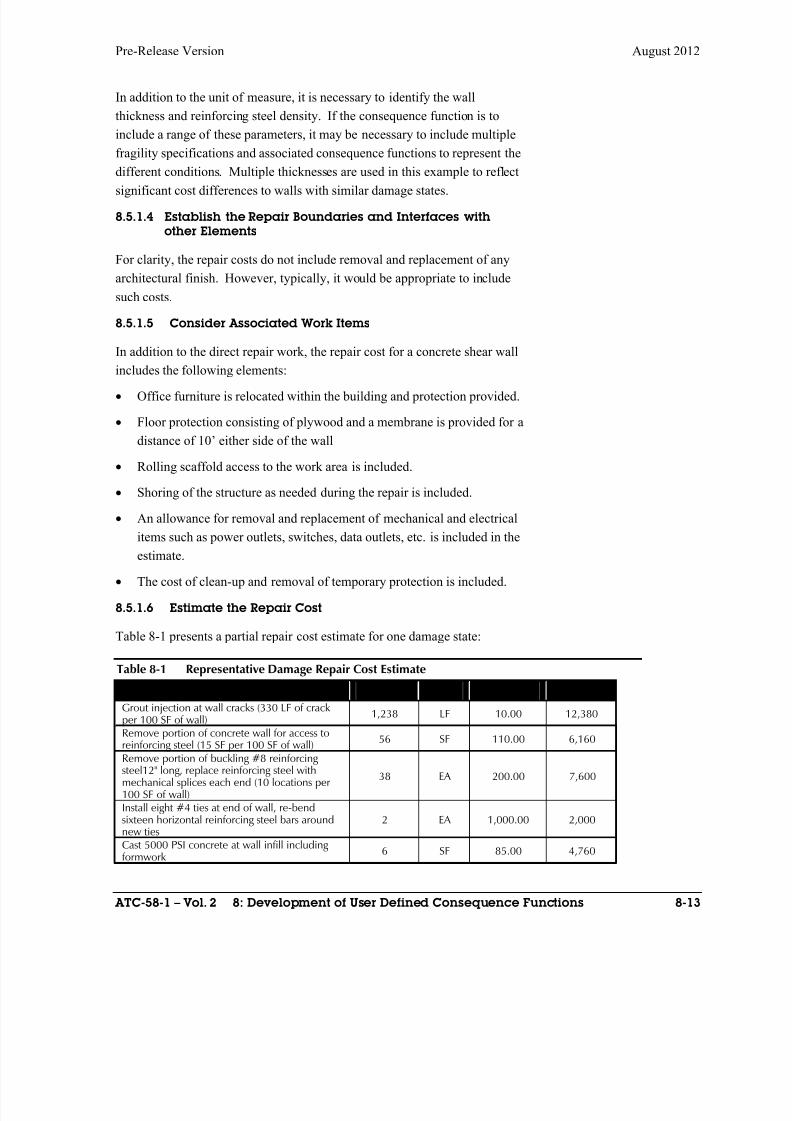
8/12/2019 Seismic Performance Assessment of Buildings
http://slidepdf.com/reader/full/seismic-performance-assessment-of-buildings 255/358
Pre-Release Version August 2012
ATC-58-1 – Vol. 2 8: Development of User Defined Consequence Functions 8-13
In addition to the unit of measure, it is necessary to identify the wall
thickness and reinforcing steel density. If the consequence function is to
include a range of these parameters, it may be necessary to include multiple
fragility specifications and associated consequence functions to represent the
different conditions. Multiple thicknesses are used in this example to reflect
significant cost differences to walls with similar damage states.
8.5.1.4 Establish the Repair Boundaries and Interfaces with
other Elements
For clarity, the repair costs do not include removal and replacement of any
architectural finish. However, typically, it would be appropriate to include
such costs.
8.5.1.5 Consider Associated Work Items
In addition to the direct repair work, the repair cost for a concrete shear wall
includes the following elements:
Office furniture is relocated within the building and protection provided.
Floor protection consisting of plywood and a membrane is provided for a
distance of 10’ either side of the wall
Rolling scaffold access to the work area is included.
Shoring of the structure as needed during the repair is included.
An allowance for removal and replacement of mechanical and electrical
items such as power outlets, switches, data outlets, etc. is included in the
estimate.
The cost of clean-up and removal of temporary protection is included.
8.5.1.6 Estimate the Repair Cost
Table 8-1 presents a partial repair cost estimate for one damage state:
Table 8-1 Representative Damage Repair Cost Estimate
Wall repairs Quantity Unit Rate Extension
Grout injection at wall cracks (330 LF of crackper 100 SF of wall)
1,238 LF 10.00 12,380
Remove portion of concrete wall for access toreinforcing steel (15 SF per 100 SF of wall) 56 SF 110.00 6,160
Remove portion of buckling #8 reinforcingsteel12" long, replace reinforcing steel withmechanical splices each end (10 locations per100 SF of wall)
38 EA 200.00 7,600
Install eight #4 ties at end of wall, re-bendsixteen horizontal reinforcing steel bars aroundnew ties
2 EA 1,000.00 2,000
Cast 5000 PSI concrete at wall infill includingformwork
6 SF 85.00 4,760
8/12/2019 Seismic Performance Assessment of Buildings
http://slidepdf.com/reader/full/seismic-performance-assessment-of-buildings 256/358
August 2012 Pre-Release Version
8-14 8: User-Defined Consequence Functions FEMA P-58 – Vol. 2
8.5.2 Establish Cost Ranges
8.5.2.1 Establish Cost Distribution
Cost ranges are established for each line item based on a three point
estimating approach, using high, low and best-estimate values. The range
can address both quantity and price uncertainty. For example, furniturerelocation is estimated at $1,000 for the best estimate value, with a range
from $500 to $3,000. Boundary reinforcing is estimated at $2,000 for the
median value, with a range of $0, representing no boundary damage to
$4,000, representing extensive boundary damage. The itemized range of
numbers are then summed to give an overall cost range. The line item high
and low values are set at 25th percentile and 75th percentile costs as opposed
to 10/90 or 0/100 percentiles to avoid setting the ranges too wide during
summing.
The dispersion, , value is set based on review of the resulting three pointestimate. For user-generated fragility specifications, it is possible to use an
overall estimate, without first calculating the three point estimate,
depending on user comfort with range estimates.
8.5.2.2 Establish Quantity Ranges where Appropriate
Baseline estimate pricing and efficiencies assumed four to ten walls being
repaired. Fewer than four walls would result in lower efficiency and
increased waste due to short orders. More than ten walls would lead to
increases in efficiency of operations. The costs for wall counts below four
increase by 20%, and the costs for walls counts above ten are decreased by20%. Adjustments are reviewed for each wall configuration considered. For
all shear wall components, the percentage increase in cost due to small
quantities ranges from 5% to 40%, and the percentage decrease for large
quantities ranges from 0% to 20%.
8.5.3 Establish Time Estimates
8.5.3.1 Establish Baseline Time Estimate
For the above example, labor hours are estimated by line item, resulting in a
median estimate of 94 hours for the repair.
8.6 Other Considerations
8.6.1 Time and Location Adjustments
User-defined consequence functions should reflect the time and location
under consideration for the PACT assessment. User-defined consequence
functions are not adjusted by time or location factors built into PACT. This
8/12/2019 Seismic Performance Assessment of Buildings
http://slidepdf.com/reader/full/seismic-performance-assessment-of-buildings 257/358
Pre-Release Version August 2012
ATC-58-1 – Vol. 2 8: Development of User Defined Consequence Functions 8-15
means that if the user-defined estimate is to be used in a later iteration or a
different location, it must be adjusted by the user to reflect these changes.
8.6.2 Double Counting
Careful consideration needs to be given to the potential for double counting
repair costs. For lower damage states, repair costs to nonstructural
components generally dominate total repair costs and damage to the
surrounding structural components are minimal. As the damage increases for
structural components, the associated repair costs may include the removal
and replacement of nonstructural components that are very likely to have
been directly damaged. The repair costs for structural components should
discount the cost of removal and replacement of adjacent nonstructural
components such as partitions, ceilings, etc. This discount acknowledges
that the repair and replacement costs of the nonstructural items will likely be
included in total repair costs through their own performance groupconsequence function.

8/12/2019 Seismic Performance Assessment of Buildings
http://slidepdf.com/reader/full/seismic-performance-assessment-of-buildings 258/358
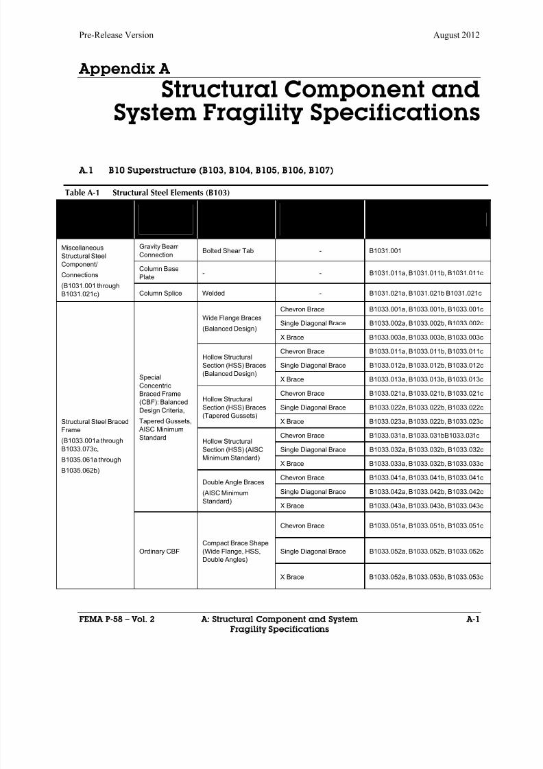
8/12/2019 Seismic Performance Assessment of Buildings
http://slidepdf.com/reader/full/seismic-performance-assessment-of-buildings 259/358
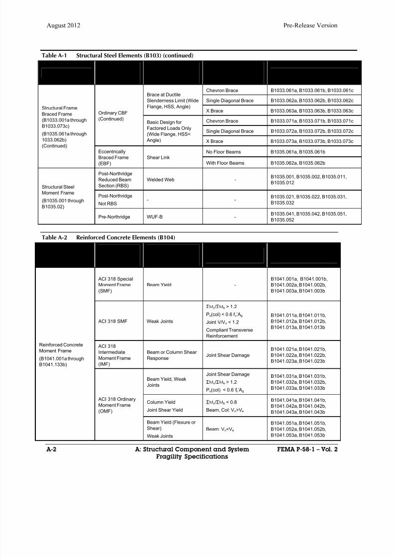
8/12/2019 Seismic Performance Assessment of Buildings
http://slidepdf.com/reader/full/seismic-performance-assessment-of-buildings 260/358
August 2012 Pre-Release Version
A-2 A: Structural Component and System FEMA P-58-1 – Vol. 2
Fragility Specifications
Table A-1 Structural Steel Elements (B103) (continued)
Material/System
Construction
Design
Characteristics
Damage Mode, Design
Configuration; Other
features
Other/
Comments/
Notes
Fragility Classification Number
Structural Frame
Braced Frame
(B1033.001a through
B1033.073c)
(B1035.061a through
1033.062b)
(Continued)
Ordinary CBF
(Continued)
Brace at Ductile
Slenderness Limit (Wide
Flange, HSS, Angle)
Chevron Brace B1033.061a, B1033.061b, B1033.061c
Single Diagonal Brace B1033.062a, B1033.062b, B1033.062c
X Brace B1033.063a, B1033.063b, B1033.063c
Basic Design for
Factored Loads Only
(Wide Flange, HSS<
Angle)
Chevron Brace B1033.071a, B1033.071b, B1033.071c
Single Diagonal Brace B1033.072a, B1033.072b, B1033.072c
X Brace B1033.073a, B1033.073b, B1033.073c
Eccentrically
Braced Frame
(EBF)
Shear LinkNo Floor Beams B1035.061a, B1035.061b
With Floor Beams B1035.062a, B1035.062b
Structural Steel
Moment Frame
(B1035.001 through
B1035.02)
Post-Northridge
Reduced Beam
Section (RBS)
Welded Web -B1035.001, B1035.002, B1035.011,
B1035.012
Post-Northridge
Not RBS- -
B1035.021, B1035.022, B1035.031,
B1035.032
Pre-Northridge WUF-B -B1035.041, B1035.042, B1035.051,
B1035.052
Table A-2 Reinforced Concrete Elements (B104)
Material/System
Construction
Design
Characteristics
Damage Mode, Design
Configuration; Other
features
Other/Comments/
Notes
Fragility Classification
Number
Reinforced Concrete
Moment Frame
(B1041.001a through
B1041.133b)
ACI 318 Special
Moment Frame
(SMF)
Beam Yield -
B1041.001a, B1041.001b,
B1041.002a, B1041.002b,
B1041.003a, B1041.003b
ACI 318 SMF Weak Joints
ΣMc/ΣMb > 1.2
Pu(col) < 0.6 f c’Ag
Joint V/Vn < 1.2
Compliant Transverse
Reinforcement
B1041.011a, B1041.011b,
B1041.012a, B1041.012b,
B1041.013a, B1041.013b
ACI 318
Intermediate
Moment Frame
(IMF)
Beam or Column Shear
ResponseJoint Shear Damage
B1041.021a, B1041.021b,
B1041.022a, B1041.022b,
B1041.023a, B1041.023b
ACI 318 Ordinary
Moment Frame
(OMF)
Beam Yield, Weak
Joints
Joint Shear Damage
ΣMc/ΣMb > 1.2
Pu(col) < 0.6 f c’Ag
B1041.031a, B1041.031b,
B1041.032a, B1041.032b,
B1041.033a, B1041.033b
Column Yield
Joint Shear Yield
ΣMc/ΣMb < 0.8
Beam, Col: Vn>Ve
B1041.041a, B1041.041b,
B1041.042a, B1041.042b,
B1041.043a, B1041.043b
Beam Yield (Flexure or
Shear)
Weak Joints
Beam: Vn<Ve
B1041.051a, B1041.051b,
B1041.052a, B1041.052b,
B1041.053a, B1041.053b

8/12/2019 Seismic Performance Assessment of Buildings
http://slidepdf.com/reader/full/seismic-performance-assessment-of-buildings 261/358
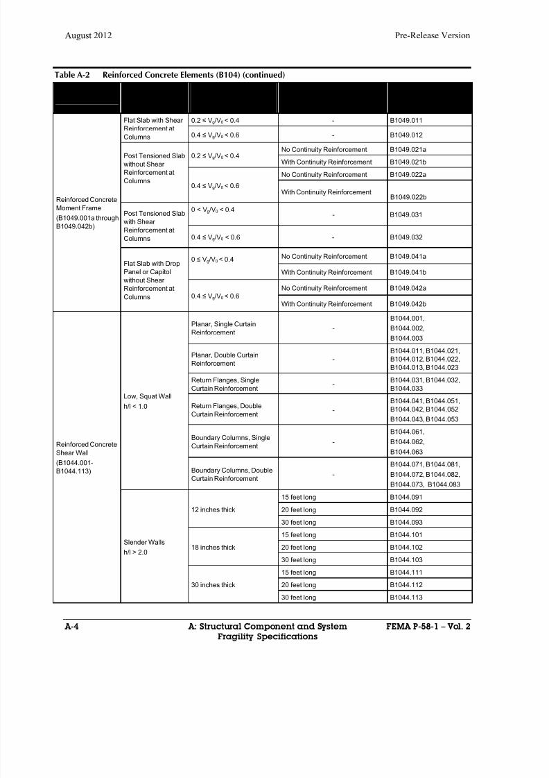
8/12/2019 Seismic Performance Assessment of Buildings
http://slidepdf.com/reader/full/seismic-performance-assessment-of-buildings 262/358
August 2012 Pre-Release Version
A-4 A: Structural Component and System FEMA P-58-1 – Vol. 2
Fragility Specifications
Table A-2 Reinforced Concrete Elements (B104) (continued)
Material/System
Construction
Design
Characteristics
Damage Mode, Design
Configuration; Other
features
Other/Comments/
Notes
Fragility Classification
Number
Reinforced Concrete
Moment Frame
(B1049.001a through
B1049.042b)
Flat Slab with Shear
Reinforcement atColumns
0.2 ≤ Vg/V0 < 0.4 - B1049.011
0.4 ≤ Vg/V0 < 0.6 - B1049.012
Post Tensioned Slab
without Shear
Reinforcement at
Columns
0.2 ≤ Vg/V0 < 0.4No Continuity Reinforcement B1049.021a
With Continuity Reinforcement B1049.021b
0.4 ≤ Vg/V0 < 0.6
No Continuity Reinforcement B1049.022a
With Continuity ReinforcementB1049.022b
Post Tensioned Slab
with Shear
Reinforcement at
Columns
0 < Vg/V0 < 0.4- B1049.031
0.4 ≤ Vg/V0 < 0.6 - B1049.032
Flat Slab with Drop
Panel or Capitol
without Shear
Reinforcement at
Columns
0 ≤ Vg/V0 < 0.4 No Continuity Reinforcement B1049.041a
With Continuity Reinforcement B1049.041b
0.4 ≤ Vg/V0 < 0.6
No Continuity Reinforcement B1049.042a
With Continuity Reinforcement B1049.042b
Reinforced Concrete
Shear Wall
(B1044.001-
B1044.113)
Low, Squat Wall
h/l < 1.0
Planar, Single Curtain
Reinforcement-
B1044.001,
B1044.002,
B1044.003
Planar, Double Curtain
Reinforcement-
B1044.011, B1044.021,
B1044.012, B1044.022,
B1044.013, B1044.023
Return Flanges, SingleCurtain Reinforcement - B1044.031, B1044.032,B1044.033
Return Flanges, Double
Curtain Reinforcement-
B1044.041, B1044.051,
B1044.042, B1044.052
B1044.043, B1044.053
Boundary Columns, Single
Curtain Reinforcement-
B1044.061,
B1044.062,
B1044.063
Boundary Columns, Double
Curtain Reinforcement-
B1044.071, B1044.081,
B1044.072, B1044.082,
B1044.073, B1044.083
Slender Walls
h/l > 2.0
12 inches thick
15 feet long B1044.091
20 feet long B1044.092
30 feet long B1044.093
18 inches thick
15 feet long B1044.101
20 feet long B1044.102
30 feet long B1044.103
30 inches thick
15 feet long B1044.111
20 feet long B1044.112
30 feet long B1044.113
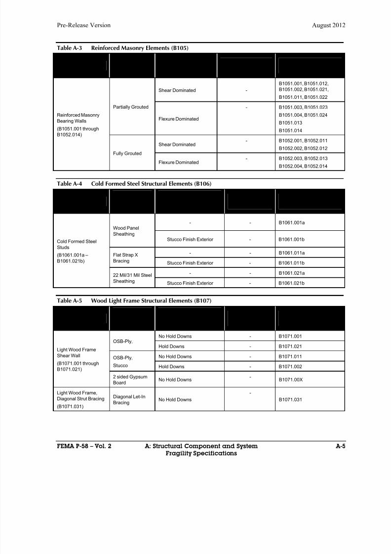
8/12/2019 Seismic Performance Assessment of Buildings
http://slidepdf.com/reader/full/seismic-performance-assessment-of-buildings 263/358
Pre-Release Version August 2012
FEMA P-58 – Vol. 2 A: Structural Component and System A-5
Fragility Specifications
Table A-3 Reinforced Masonry Elements (B105)
Material/System
Construction
Design
Characteristics
Damage Mode, Design
Configuration; Other
features
Other/Comments/Note
s
Fragility Classification
Number
Reinforced Masonry
Bearing Walls
(B1051.001 through
B1052.014)
Partially Grouted
Shear Dominated -
B1051.001, B1051.012,
B1051.002, B1051.021,B1051.011, B1051.022
Flexure Dominated
- B1051.003, B1051.023
B1051.004, B1051.024
B1051.013
B1051.014
Fully Grouted
Shear Dominated- B1052.001, B1052.011
B1052.002, B1052.012
Flexure Dominated- B1052.003, B1052.013
B1052.004, B1052.014
Table A-4 Cold Formed Steel Structural Elements (B106)
Material/System
Construction
Design
Characteristics
Damage Mode, Design
Configuration; Other
features
Other/Comments/N
otes
Fragility Classification
Number
Cold Formed Steel
Studs
(B1061.001a –
B1061.021b)
Wood Panel
Sheathing
- - B1061.001a
Stucco Finish Exterior - B1061.001b
Flat Strap X
Bracing
- - B1061.011a
Stucco Finish Exterior - B1061.011b
22 Mil/31 Mil Steel
Sheathing
- - B1061.021a
Stucco Finish Exterior - B1061.021b
Table A-5 Wood Light Frame Structural Elements (B107)
Material/System
Construction
Design
Characteristics
Damage Mode, Design
Configuration; Other
features
Other/Comments/N
otes
Fragility Classification
Number
Light Wood Frame
Shear Wall
(B1071.001 throughB1071.021)
OSB-Ply,No Hold Downs - B1071.001
Hold Downs - B1071.021
OSB-Ply,
Stucco
No Hold Downs - B1071.011
Hold Downs - B1071.002
2 sided Gypsum
BoardNo Hold Downs
-B1071.00X
Light Wood Frame,
Diagonal Strut Bracing
(B1071.031)
Diagonal Let-In
BracingNo Hold Downs
-
B1071.031

8/12/2019 Seismic Performance Assessment of Buildings
http://slidepdf.com/reader/full/seismic-performance-assessment-of-buildings 264/358
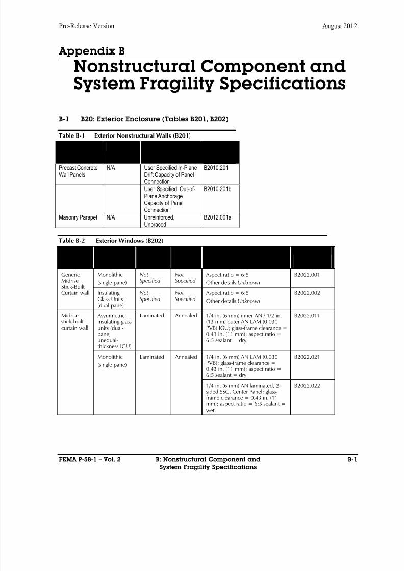
8/12/2019 Seismic Performance Assessment of Buildings
http://slidepdf.com/reader/full/seismic-performance-assessment-of-buildings 265/358
Pre-Release Version August 2012
FEMA P-58-1 – Vol. 2 B: Nonstructural Component and B-1
System Fragility Specifications
Appendix B
Nonstructural Component andSystem Fragility Specifications
B-1 B20: Exterior Enclosure (Tables B201, B202)
Table B-1 Exterior Nonstructural Walls (B201)
ItemDescription
Size Seismic installationcondition
FragilityClassificationNumber
Precast ConcreteWall Panels
N/A User Specified In-PlaneDrift Capacity of PanelConnection
B2010.201
User Specified Out-of-Plane AnchorageCapacity of PanelConnection
B2010.201b
Masonry Parapet N/A Unreinforced,Unbraced
B2012.001a
Table B-2 Exterior Windows (B202)
Basic type Configuration Laminated? Glasstype
Details FragilityClassificationNumber
Generic
MidriseStick-BuiltCurtain wall
Monolithic
(single pane)
Not
Specified
Not
Specified
Aspect ratio = 6:5
Other details Unknown
B2022.001
InsulatingGlass Units(dual pane)
NotSpecified
NotSpecified
Aspect ratio = 6:5
Other details Unknown
B2022.002
Midrisestick-builtcurtain wall
Asymmetricinsulating glassunits (dual-pane,unequal-thickness IGU)
Laminated Annealed 1/4 in. (6 mm) inner AN / 1/2 in.(13 mm) outer AN LAM (0.030PVB) IGU; glass-frame clearance =0.43 in. (11 mm); aspect ratio =6:5 sealant = dry
B2022.011
Monolithic
(single pane)
Laminated Annealed 1/4 in. (6 mm) AN LAM (0.030PVB); glass-frame clearance =0.43 in. (11 mm); aspect ratio =
6:5 sealant = dry
B2022.021
1/4 in. (6 mm) AN laminated, 2-sided SSG, Center Panel; glass-frame clearance = 0.43 in. (11mm); aspect ratio = 6:5 sealant =wet
B2022.022

8/12/2019 Seismic Performance Assessment of Buildings
http://slidepdf.com/reader/full/seismic-performance-assessment-of-buildings 266/358
August 2012 Pre-Release Version
B-2 B: Nonstructural Component and FEMA P-58-1 – Vol. 2
System Fragility Specifications
Table B-2 Exterior Windows (B202) (continued)
Basic type Configuration Laminated? Glasstype
Details FragilityClassificationNumber
1/4 in. (6 mm) AN laminated, 2-sided SSG, Outside Panel; glass-frame clearance = 0.43 in. (11mm); aspect ratio = 6:5 sealant =wet
B2022.023
Midrisestick-builtcurtain wall
Monolithic
(single pane)
Notlaminated
Annealed 1/4 in. (6 mm) AN monolithic;glass-frame clearance = 0.43 in.(11 mm); aspect ratio = 6:5sealant = dry
B2022.031
1/4 in. (6 mm) AN monolithic;glass-frame clearance = 0 in. (0mm); aspect ratio = 6:5 sealant =dry
B2022.032
1/4 in. (6 mm) AN monolithic;glass-frame clearance = 0.13 in. (3
mm); aspect ratio = 6:5 sealant =dry
B2022.033
1/4 in. (6 mm) AN monolithic;glass-frame clearance = 0.25 in. (6mm); aspect ratio = 6:5 sealant =dry
B2022.034
1/4 in. (6 mm) AN monolithic;glass-frame clearance = 0.43 in.(11 mm); aspect ratio = 2:1sealant = dry
B2022.035
1/4 in. (6 mm) AN monolithic;glass-frame clearance = 0.43 in.(11 mm); aspect ratio = 1:2
sealant = dry
B2022.036
1/4 in. (6 mm) AN monolithic, 2-sided SSG, Center Panel; glass-frame clearance = 0.43 in. (11mm); aspect ratio = 6:5 sealant =wet
B2022.037
1/4 in. (6 mm) AN monolithic, 2-sided SSG, Outside Panel; glass-frame clearance = 0.43 in. (11mm); aspect ratio = 6:5 sealant =wet
B2022.038
1/4 in. (6 mm) AN monolithic;glass-frame clearance = 0.43 in.
(11 mm); aspect ratio = 6:5sealant = dry
B2022.039
1/4 in. (6 mm) AN monolithic;glass-frame clearance = 0.43 in.(11 mm); aspect ratio = 2:1sealant = dry
B2022.040
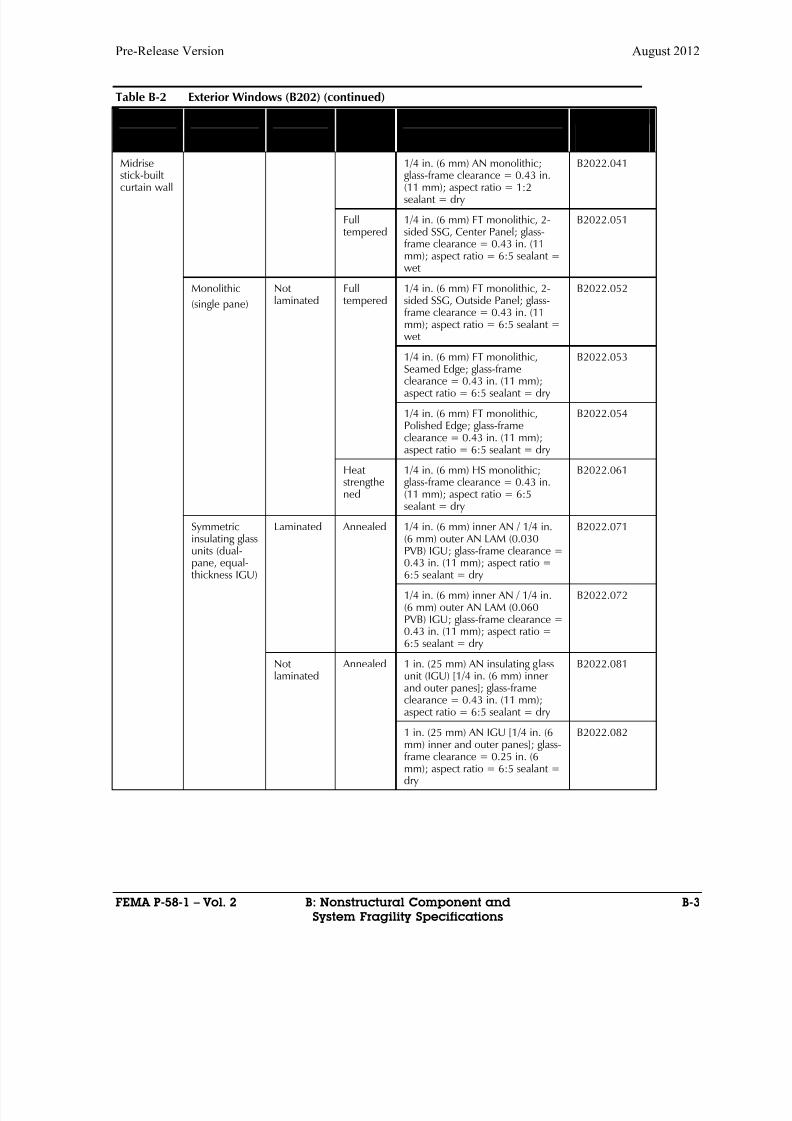
8/12/2019 Seismic Performance Assessment of Buildings
http://slidepdf.com/reader/full/seismic-performance-assessment-of-buildings 267/358
Pre-Release Version August 2012
FEMA P-58-1 – Vol. 2 B: Nonstructural Component and B-3
System Fragility Specifications
Table B-2 Exterior Windows (B202) (continued)
Basic type Configuration Laminated? Glasstype
Details FragilityClassificationNumber
Midrisestick-builtcurtain wall
1/4 in. (6 mm) AN monolithic;glass-frame clearance = 0.43 in.(11 mm); aspect ratio = 1:2sealant = dry
B2022.041
Fulltempered
1/4 in. (6 mm) FT monolithic, 2-sided SSG, Center Panel; glass-frame clearance = 0.43 in. (11mm); aspect ratio = 6:5 sealant =wet
B2022.051
Monolithic
(single pane)
Notlaminated
Fulltempered
1/4 in. (6 mm) FT monolithic, 2-sided SSG, Outside Panel; glass-frame clearance = 0.43 in. (11mm); aspect ratio = 6:5 sealant =wet
B2022.052
1/4 in. (6 mm) FT monolithic,
Seamed Edge; glass-frameclearance = 0.43 in. (11 mm);aspect ratio = 6:5 sealant = dry
B2022.053
1/4 in. (6 mm) FT monolithic,Polished Edge; glass-frameclearance = 0.43 in. (11 mm);aspect ratio = 6:5 sealant = dry
B2022.054
Heatstrengthened
1/4 in. (6 mm) HS monolithic;glass-frame clearance = 0.43 in.(11 mm); aspect ratio = 6:5sealant = dry
B2022.061
Symmetricinsulating glass
units (dual-pane, equal-thickness IGU)
Laminated Annealed 1/4 in. (6 mm) inner AN / 1/4 in.(6 mm) outer AN LAM (0.030
PVB) IGU; glass-frame clearance =0.43 in. (11 mm); aspect ratio =6:5 sealant = dry
B2022.071
1/4 in. (6 mm) inner AN / 1/4 in.(6 mm) outer AN LAM (0.060PVB) IGU; glass-frame clearance =0.43 in. (11 mm); aspect ratio =6:5 sealant = dry
B2022.072
Notlaminated
Annealed 1 in. (25 mm) AN insulating glassunit (IGU) [1/4 in. (6 mm) innerand outer panes]; glass-frameclearance = 0.43 in. (11 mm);aspect ratio = 6:5 sealant = dry
B2022.081
1 in. (25 mm) AN IGU [1/4 in. (6mm) inner and outer panes]; glass-frame clearance = 0.25 in. (6mm); aspect ratio = 6:5 sealant =dry
B2022.082
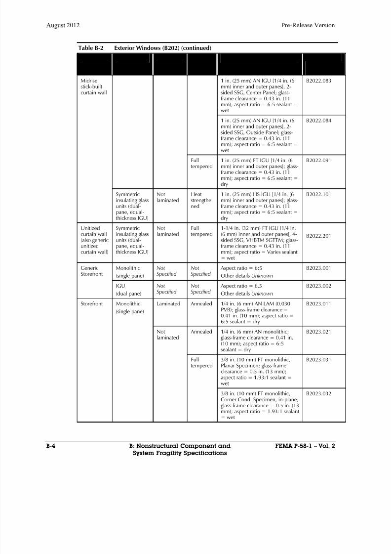
8/12/2019 Seismic Performance Assessment of Buildings
http://slidepdf.com/reader/full/seismic-performance-assessment-of-buildings 268/358
August 2012 Pre-Release Version
B-4 B: Nonstructural Component and FEMA P-58-1 – Vol. 2
System Fragility Specifications
Table B-2 Exterior Windows (B202) (continued)
Basic type Configuration Laminated? Glasstype
Details FragilityClassificationNumber
Midrisestick-builtcurtain wall
1 in. (25 mm) AN IGU [1/4 in. (6mm) inner and outer panes], 2-sided SSG, Center Panel; glass-frame clearance = 0.43 in. (11mm); aspect ratio = 6:5 sealant =wet
B2022.083
1 in. (25 mm) AN IGU [1/4 in. (6mm) inner and outer panes], 2-sided SSG, Outside Panel; glass-frame clearance = 0.43 in. (11mm); aspect ratio = 6:5 sealant =wet
B2022.084
Fulltempered
1 in. (25 mm) FT IGU [1/4 in. (6mm) inner and outer panes]; glass-frame clearance = 0.43 in. (11mm); aspect ratio = 6:5 sealant =dry
B2022.091
Symmetricinsulating glassunits (dual-pane, equal-thickness IGU)
Notlaminated
Heatstrengthened
1 in. (25 mm) HS IGU [1/4 in. (6mm) inner and outer panes]; glass-frame clearance = 0.43 in. (11mm); aspect ratio = 6:5 sealant =dry
B2022.101
Unitizedcurtain wall(also genericunitizedcurtain wall)
Symmetricinsulating glassunits (dual-pane, equal-thickness IGU)
Notlaminated
Fulltempered
1-1/4 in. (32 mm) FT IGU [1/4 in.(6 mm) inner and outer panes], 4-sided SSG, VHBTM SGTTM; glass-frame clearance = 0.43 in. (11mm); aspect ratio = Varies sealant= wet
B2022.201
GenericStorefront
Monolithic
(single pane)
NotSpecified
NotSpecified
Aspect ratio = 6:5
Other details Unknown
B2023.001
IGU
(dual pane)
NotSpecified
NotSpecified
Aspect ratio = 6.5
Other details Unknown
B2023.002
Storefront Monolithic
(single pane)
Laminated Annealed 1/4 in. (6 mm) AN LAM (0.030PVB); glass-frame clearance =0.41 in. (10 mm); aspect ratio =6:5 sealant = dry
B2023.011
Notlaminated
Annealed 1/4 in. (6 mm) AN monolithic;glass-frame clearance = 0.41 in.(10 mm); aspect ratio = 6:5sealant = dry
B2023.021
Fulltempered
3/8 in. (10 mm) FT monolithic,Planar Specimen; glass-frameclearance = 0.5 in. (13 mm);aspect ratio = 1.93:1 sealant =wet
B2023.031
3/8 in. (10 mm) FT monolithic,Corner Cond. Specimen, in-plane;glass-frame clearance = 0.5 in. (13mm); aspect ratio = 1.93:1 sealant= wet
B2023.032
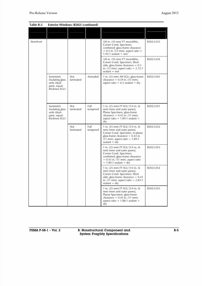
8/12/2019 Seismic Performance Assessment of Buildings
http://slidepdf.com/reader/full/seismic-performance-assessment-of-buildings 269/358
Pre-Release Version August 2012
FEMA P-58-1 – Vol. 2 B: Nonstructural Component and B-5
System Fragility Specifications
Table B-2 Exterior Windows (B202) (continued)
Basic type Configuration Laminated? Glasstype
Details FragilityClassificationNumber
Storefront 3/8 in. (10 mm) FT monolithic,Corner Cond. Specimen,combined; glass-frame clearance= 0.5 in. (13 mm); aspect ratio =1.93:1 sealant = wet
B2023.033
3/8 in. (10 mm) FT monolithic,Corner Cond. Specimen, Shortside; glass-frame clearance = 0.5in. (13 mm); aspect ratio = 2.72:1sealant = wet
B2023.034
Symmetricinsulating glassunits (dual-pane, equal-thickness IGU)
Notlaminated
Annealed 1 in. (25 mm) AN IGU; glass-frameclearance = 0.59 in. (15 mm);aspect ratio = 6:5 sealant = dry
B2023.041
Symmetricinsulating glassunits (dual-pane, equal-thickness IGU)
Notlaminated
Fulltempered
1 in. (25 mm) FT IGU [1/4 in. (6mm) inner and outer panes],Planar Specimen; glass-frameclearance = 0.43 in. (11 mm);aspect ratio = 1.89:1 sealant =dry
B2023.051
Notlaminated
Fulltempered
1 in. (25 mm) FT IGU [1/4 in. (6mm) inner and outer panes],Corner Cond. Specimen, in-plane;glass-frame clearance = 0.43 in.(11 mm); aspect ratio = 1.89:1sealant = dry
B2023.052
1 in. (25 mm) FT IGU [1/4 in. (6mm) inner and outer panes],Corner Cond. Specimen,combined; glass-frame clearance= 0.43 in. (11 mm); aspect ratio= 1.89:1 sealant = dry
B2023.053
1 in. (25 mm) FT IGU [1/4 in. (6mm) inner and outer panes],Corner Cond. Specimen, Shortside; glass-frame clearance = 0.43in. (11 mm); aspect ratio = 2.83:1sealant = dry
B2023.054
1 in. (25 mm) FT IGU [1/4 in. (6mm) inner and outer panes],Planar Specimen; glass-frameclearance = 0.43 in. (11 mm);aspect ratio = 1.88:1 sealant =dry
B2023.055
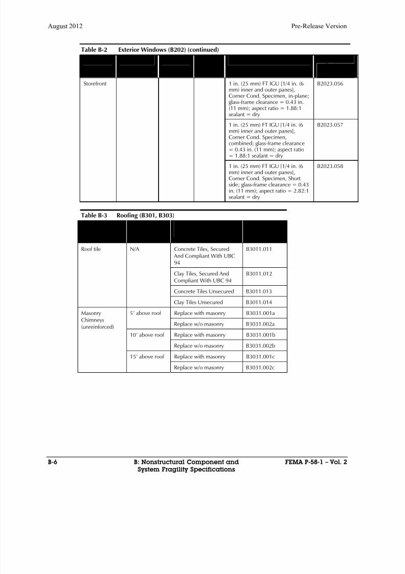
8/12/2019 Seismic Performance Assessment of Buildings
http://slidepdf.com/reader/full/seismic-performance-assessment-of-buildings 270/358
August 2012 Pre-Release Version
B-6 B: Nonstructural Component and FEMA P-58-1 – Vol. 2
System Fragility Specifications
Table B-2 Exterior Windows (B202) (continued)
Basic type Configuration Laminated? Glasstype
Details FragilityClassificationNumber
Storefront 1 in. (25 mm) FT IGU [1/4 in. (6mm) inner and outer panes],Corner Cond. Specimen, in-plane;glass-frame clearance = 0.43 in.(11 mm); aspect ratio = 1.88:1sealant = dry
B2023.056
1 in. (25 mm) FT IGU [1/4 in. (6mm) inner and outer panes],Corner Cond. Specimen,combined; glass-frame clearance= 0.43 in. (11 mm); aspect ratio= 1.88:1 sealant = dry
B2023.057
1 in. (25 mm) FT IGU [1/4 in. (6mm) inner and outer panes],Corner Cond. Specimen, Shortside; glass-frame clearance = 0.43in. (11 mm); aspect ratio = 2.82:1sealant = dry
B2023.058
Table B-3 Roofing (B301, B303)
Item Description Size Seismic installationcondition/repair approach
FragilityClassificationNumber
Roof tile N/A Concrete Tiles, Secured And Compliant With UBC94
B3011.011
Clay Tiles, Secured And
Compliant With UBC 94
B3011.012
Concrete Tiles Unsecured B3011.013
Clay Tiles Unsecured B3011.014
MasonryChimneys(unreinforced)
5’ above roof Replace with masonry B3031.001a
Replace w/o masonry B3031.002a
10’ above roof Replace with masonry B3031.001b
Replace w/o masonry B3031.002b
15’ above roof Replace with masonry B3031.001c
Replace w/o masonry B3031.002c
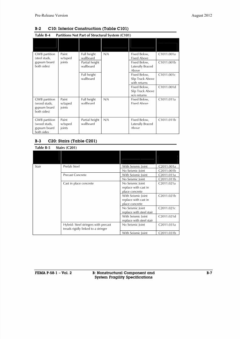
8/12/2019 Seismic Performance Assessment of Buildings
http://slidepdf.com/reader/full/seismic-performance-assessment-of-buildings 271/358
Pre-Release Version August 2012
FEMA P-58-1 – Vol. 2 B: Nonstructural Component and B-7
System Fragility Specifications
B-2 C10: Interior Construction (Table C101)
Table B-4 Partitions Not Part of Structural System (C101)
ItemDescription
Finish Full orpartialheight
Cornerconfiguration
Installationvariable
FragilityClassification Number
GWB partition(steel studs,gypsum boardboth sides)
Paintw/taped joints
Full heightwallboard N/A Fixed Below,Fixed Above C1011.001a
Partial heightwallboard
Fixed Below,Laterally Braced Above
C1011.001b
Full heightwallboard
Fixed Below,Slip Track Abovewith returns
C1011.001c
Fixed Below,Slip Track Abovew/o returns
C1011.001d
GWB partition(wood studs,gypsum board
both sides)
Paintw/taped joints
Full heightwallboard
N/A Fixed Below,Fixed Above
C1011.011a
GWB partition(wood studs,gypsum boardboth sides
Paintw/taped joints
Partial heightwallboard
N/A Fixed Below,Laterally Braced Above
C1011.011b
B-3 C20: Stairs (Table C201)
Table B-5 Stairs (C201)
ItemDescription
Type Seismic installationcondition/repairaction
FragilityClassificationNumber
Stair Prefab Steel With Seismic Joint C2011.001aNo Seismic Joint C2011.001b
Precast Concrete With Seismic Joint C2011.011a
No Seismic Joint C2011.011b
Cast in place concrete No Seismic Jointreplace with cast inplace concrete
C2011.021a
With Seismic Jointreplace with cast inplace concrete
C2011.021b
No Seismic Jointreplace with steel stair
C2011.021c
With Seismic Jointreplace with steel stair
C2011.021d
Hybrid: Steel stringers with precasttreads rigidly linked to a stringer
No Seismic Joint C2011.031a
With Seismic Joint C2011.031b
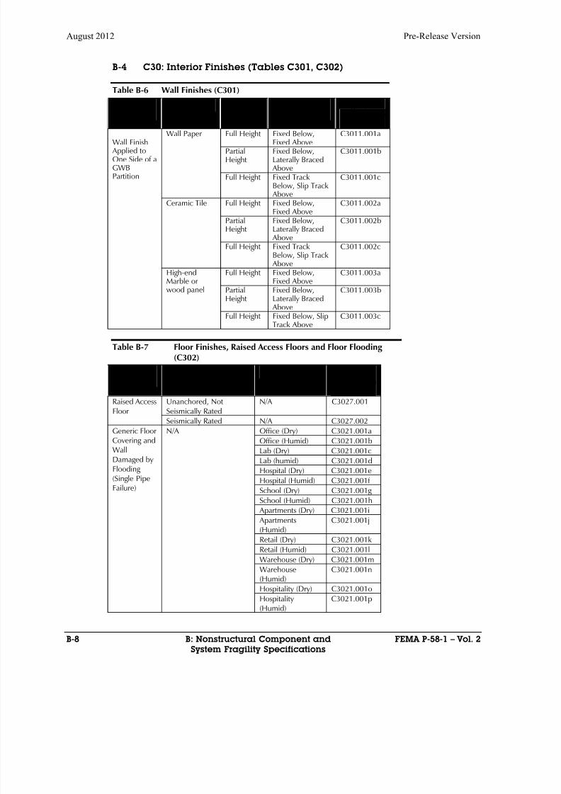
8/12/2019 Seismic Performance Assessment of Buildings
http://slidepdf.com/reader/full/seismic-performance-assessment-of-buildings 272/358
August 2012 Pre-Release Version
B-8 B: Nonstructural Component and FEMA P-58-1 – Vol. 2
System Fragility Specifications
B-4 C30: Interior Finishes (Tables C301, C302)
Table B-6 Wall Finishes (C301)
ItemDescription
Finish Full orPartialHeight
Installation Variable
FragilityClassificationNumber
Wall Finish Applied toOne Side of aGWBPartition
Wall Paper Full Height Fixed Below,Fixed Above
C3011.001a
PartialHeight
Fixed Below,Laterally Braced Above
C3011.001b
Full Height Fixed TrackBelow, Slip Track Above
C3011.001c
Ceramic Tile Full Height Fixed Below,Fixed Above
C3011.002a
PartialHeight
Fixed Below,Laterally Braced Above
C3011.002b
Full Height Fixed TrackBelow, Slip Track Above
C3011.002c
High-endMarble orwood panel
Full Height Fixed Below,Fixed Above
C3011.003a
PartialHeight
Fixed Below,Laterally Braced Above
C3011.003b
Full Height Fixed Below, SlipTrack Above
C3011.003c
Table B-7 Floor Finishes, Raised Access Floors and Floor Flooding(C302)
ItemDescription
Seismic InstallationCondition
Size/Other FragilityClassification
NumberRaised AccessFloor
Unanchored, NotSeismically Rated
N/A C3027.001
Seismically Rated N/A C3027.002
Generic FloorCovering andWallDamaged byFlooding(Single PipeFailure)
N/A Office (Dry) C3021.001a
Office (Humid) C3021.001b
Lab (Dry) C3021.001c
Lab (humid) C3021.001d
Hospital (Dry) C3021.001e
Hospital (Humid) C3021.001f
School (Dry) C3021.001g
School (Humid) C3021.001h
Apartments (Dry) C3021.001i
Apartments(Humid)
C3021.001j
Retail (Dry) C3021.001k
Retail (Humid) C3021.001l
Warehouse (Dry) C3021.001m
Warehouse(Humid)
C3021.001n
Hospitality (Dry) C3021.001o
Hospitality(Humid)
C3021.001p

8/12/2019 Seismic Performance Assessment of Buildings
http://slidepdf.com/reader/full/seismic-performance-assessment-of-buildings 273/358
Pre-Release Version August 2012
FEMA P-58-1 – Vol. 2 B: Nonstructural Component and B-9
System Fragility Specifications
Table B-8 Suspended Ceiling and Ceiling Lighting (C303)
Item Description Seismic InstallationCondition
Size/Area FragilityClassificationNumber
Suspended
Ceiling
SDC: A,B Vertical support
only
< 250 SF C3032.001a
250 – 1000 SF C3032.001b1000 – 2500SF
C3032.001c
>2500 SF C3032.001d
SDC C: Vertical supportand lateral support forlarger ceiling areas
< 250 SF C3032.002a
250 – 1000 SF C3032.002b
1000 – 2500SF
C3032.002c
>2500 SF C3032.002d
SDC D/E: (Ip=1.0) verticaland lateral support lateralsupport for larger ceilingareas plus wider perimeter
angle.
< 250 SF C3032.003a
250 – 1000 SF C3032.003b
1000 – 2500SF
C3032.003c
>2500 SF C3032.003dSDC: D,E,F (Ip=1.5)Same as D/E plus stringentdesign and installationQ/C
< 250 SF C3032.004a
250 – 1000 SF C3032.004b
1000 – 2500SF
C3032.004c
>2500 SF C3032.004d
Recessed Lightingin SuspendedCeiling
No independent supportwires
C3032.001a
Recessed Lightingin SuspendedCeiling
With IndependentSupport wires
C3032.002
IndependentPendant Lighting
Not seismically rated C3034.001
IndependentPendant Lighting
Seismically rated C3034.002
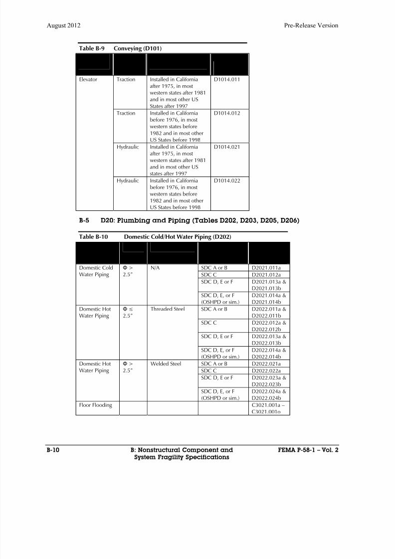
8/12/2019 Seismic Performance Assessment of Buildings
http://slidepdf.com/reader/full/seismic-performance-assessment-of-buildings 274/358
August 2012 Pre-Release Version
B-10 B: Nonstructural Component and FEMA P-58-1 – Vol. 2
System Fragility Specifications
Table B-9 Conveying (D101)
ItemDescription
Type Seismic installationcondition
FragilityClassificationNumber
Elevator Traction Installed in Californiaafter 1975, in most
western states after 1981and in most other USStates after 1997
D1014.011
Traction Installed in Californiabefore 1976, in mostwestern states before1982 and in most otherUS States before 1998
D1014.012
Hydraulic Installed in Californiaafter 1975, in mostwestern states after 1981and in most other USstates after 1997
D1014.021
Hydraulic Installed in Californiabefore 1976, in mostwestern states before1982 and in most otherUS States before 1998
D1014.022
B-5 D20: Plumbing and Piping (Tables D202, D203, D205, D206)
Table B-10 Domestic Cold/Hot Water Piping (D202)
System/ItemDescription
Size Material Type Installation Variable
FragilityClassificationNumber
Domestic Cold
Water Piping
Φ >
2.5”
N/A SDC A or B D2021.011a
SDC C D2021.012aSDC D, E or F D2021.013a &
D2021.013b
SDC D, E, or F(OSHPD or sim.)
D2021.014a &D2021.014b
Domestic HotWater Piping
Φ ≤ 2.5”
Threaded Steel SDC A or B D2022.011a &D2022.011b
SDC C D2022.012a &D2022.012b
SDC D, E or F D2022.013a &D2022.013b
SDC D, E, or F(OSHPD or sim.)
D2022.014a &D2022.014b
Domestic HotWater PipingΦ
>2.5” Welded Steel SDC A or B D2022.021aSDC C D2022.022a
SDC D, E or F D2022.023a &D2022.023b
SDC D, E, or F(OSHPD or sim.)
D2022.024a &D2022.024b
Floor Flooding C3021.001a –C3021.001o
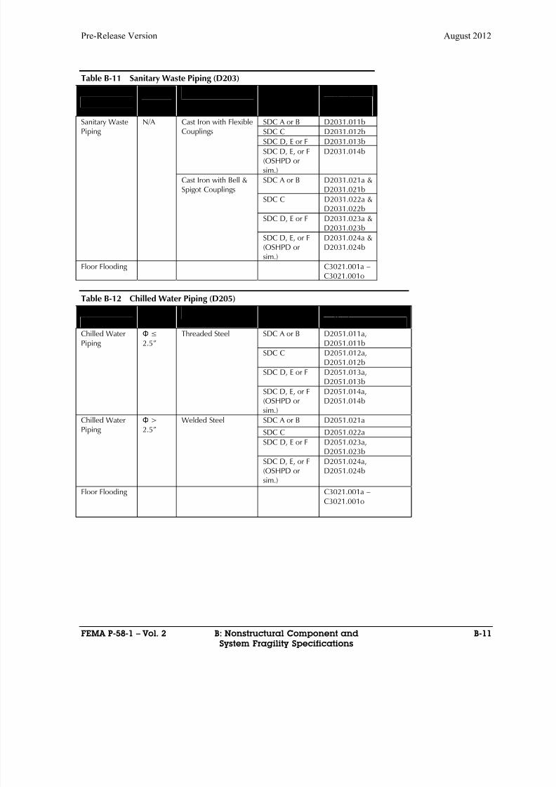
8/12/2019 Seismic Performance Assessment of Buildings
http://slidepdf.com/reader/full/seismic-performance-assessment-of-buildings 275/358
Pre-Release Version August 2012
FEMA P-58-1 – Vol. 2 B: Nonstructural Component and B-11
System Fragility Specifications
Table B-11 Sanitary Waste Piping (D203)
System/ItemDescription
Size Material Type Installation Variable
FragilityClassificationNumber
Sanitary Waste
Piping
N/A Cast Iron with Flexible
Couplings
SDC A or B D2031.011b
SDC C D2031.012bSDC D, E or F D2031.013b
SDC D, E, or F(OSHPD orsim.)
D2031.014b
Cast Iron with Bell &Spigot Couplings
SDC A or B D2031.021a &D2031.021b
SDC C D2031.022a &D2031.022b
SDC D, E or F D2031.023a &D2031.023b
SDC D, E, or F(OSHPD or
sim.)
D2031.024a &D2031.024b
Floor Flooding C3021.001a –C3021.001o
Table B-12 Chilled Water Piping (D205)
System/ItemDescription
Size Material Type Installation Variable
Fragility ClassificationNumber
Chilled WaterPiping
Φ ≤ 2.5”
Threaded Steel SDC A or B D2051.011a,D2051.011b
SDC C D2051.012a,D2051.012b
SDC D, E or F D2051.013a,D2051.013b
SDC D, E, or F(OSHPD orsim.)
D2051.014a,D2051.014b
Chilled WaterPiping
Φ >2.5”
Welded Steel SDC A or B D2051.021a
SDC C D2051.022a
SDC D, E or F D2051.023a,D2051.023b
SDC D, E, or F(OSHPD orsim.)
D2051.024a,D2051.024b
Floor Flooding C3021.001a –C3021.001o
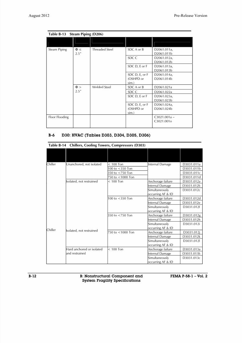
8/12/2019 Seismic Performance Assessment of Buildings
http://slidepdf.com/reader/full/seismic-performance-assessment-of-buildings 276/358
August 2012 Pre-Release Version
B-12 B: Nonstructural Component and FEMA P-58-1 – Vol. 2
System Fragility Specifications
Table B-13 Steam Piping (D206)
System/ItemDescription
Size Material Type Installation Variable
Fragility ClassificationNumber
Steam Piping Φ ≤ 2.5”
Threaded Steel SDC A or B D2061.011a,D2061.011b
SDC C D2061.012a,D2061.012b
SDC D, E or F D2061.013a,D2061.013b
SDC D, E, or F(OSHPD orsim.)
D2061.014a,D2061.014b
Φ >2.5”
Welded Steel SDC A or B D2061.021a
SDC C D2061.022a
SDC D, E or F D2061.023a,D2061.023b
SDC D, E, or F(OSHPD or
sim.)
D2061.024a,D2061.024b
Floor Flooding C3021.001a –C3021.001o
B-6 D30: HVAC (Tables D303, D304, D305, D306)
Table B-14 Chillers, Cooling Towers, Compressors (D303)
EquipmentDescription
Installation Variables Size or Rated Capacity Dominant DamageMode
FragilityClassification
Number
Chiller
Chiller
Unanchored, not isolated < 100 Ton Internal Damage D3031.011a
100 to <350 Ton D3031.011b350 to <750 Ton D3031.011c
750 to <1000 Ton D3031.011d
Isolated, not restrained
Isolated, not restrained
< 100 Ton Anchorage failure D3031.012a
Internal Damage D3031.012b
Simultaneouslyoccurring AF & ID
D3031.012c
100 to <350 Ton Anchorage failure D3031.012d
Internal Damage D3031.012e
Simultaneouslyoccurring AF & ID
D3031.012f
350 to <750 Ton Anchorage failure D3031.012g
Internal Damage D3031.012h
Simultaneouslyoccurring AF & ID D3031.012i
750 to <1000 Ton Anchorage failure D3031.012j
Internal Damage D3031.012k
Simultaneouslyoccurring AF & ID
D3031.012l
Hard anchored or isolatedand restrained
< 100 Ton Anchorage failure D3031.013a
Internal Damage D3031.013b
Simultaneouslyoccurring AF & ID
D3031.013c
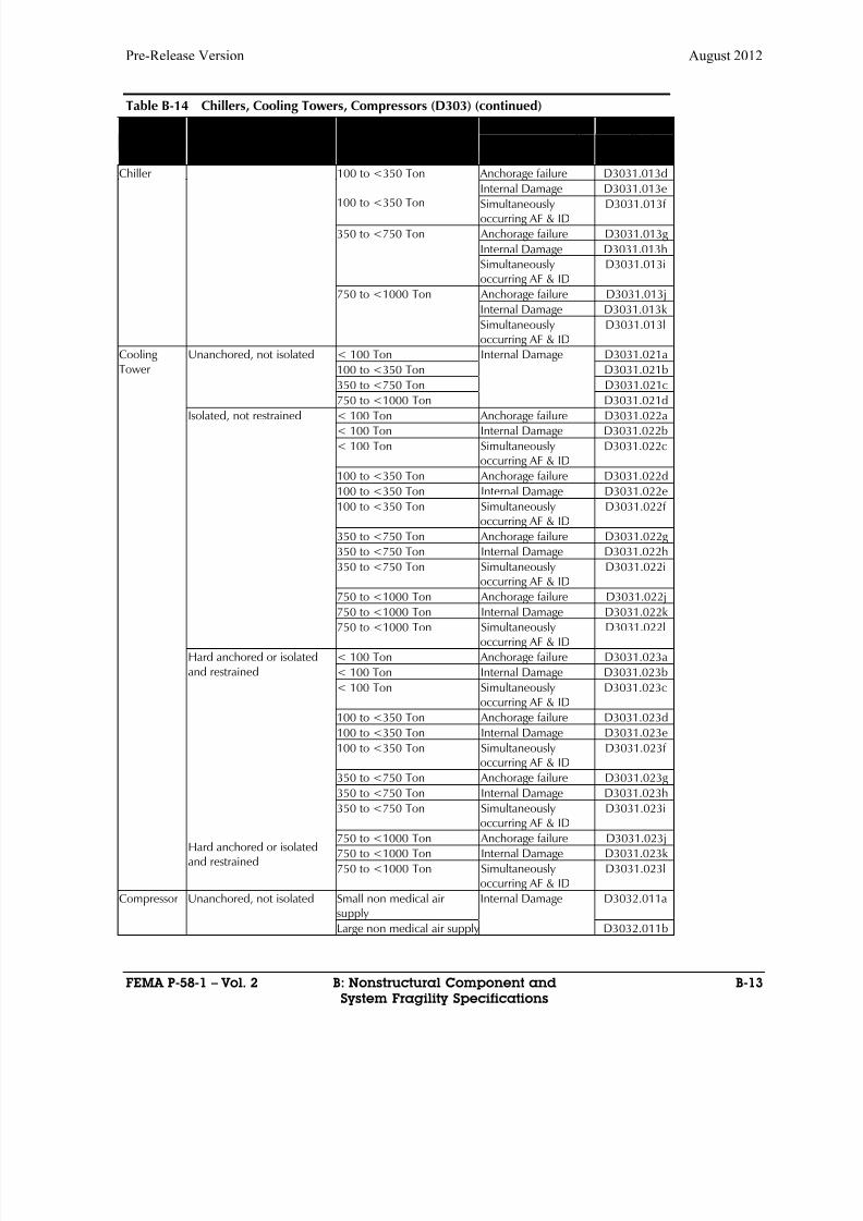
8/12/2019 Seismic Performance Assessment of Buildings
http://slidepdf.com/reader/full/seismic-performance-assessment-of-buildings 277/358
Pre-Release Version August 2012
FEMA P-58-1 – Vol. 2 B: Nonstructural Component and B-13
System Fragility Specifications
Table B-14 Chillers, Cooling Towers, Compressors (D303) (continued)
EquipmentDescription
Installation Variables Size or Rated Capacity Dominant DamageMode
FragilityClassification
Number
Chiller 100 to <350 Ton
100 to <350 Ton
Anchorage failure D3031.013d
Internal Damage D3031.013e
Simultaneouslyoccurring AF & ID
D3031.013f
350 to <750 Ton Anchorage failure D3031.013g
Internal Damage D3031.013h
Simultaneouslyoccurring AF & ID
D3031.013i
750 to <1000 Ton Anchorage failure D3031.013j
Internal Damage D3031.013k
Simultaneouslyoccurring AF & ID
D3031.013l
CoolingTower
Unanchored, not isolated < 100 Ton Internal Damage D3031.021a
100 to <350 Ton D3031.021b
350 to <750 Ton D3031.021c
750 to <1000 Ton D3031.021dIsolated, not restrained < 100 Ton Anchorage failure D3031.022a
< 100 Ton Internal Damage D3031.022b
< 100 Ton Simultaneouslyoccurring AF & ID
D3031.022c
100 to <350 Ton Anchorage failure D3031.022d
100 to <350 Ton Internal Damage D3031.022e
100 to <350 Ton Simultaneouslyoccurring AF & ID
D3031.022f
350 to <750 Ton Anchorage failure D3031.022g
350 to <750 Ton Internal Damage D3031.022h
350 to <750 Ton Simultaneouslyoccurring AF & ID
D3031.022i
750 to <1000 Ton Anchorage failure D3031.022j750 to <1000 Ton Internal Damage D3031.022k
750 to <1000 Ton Simultaneouslyoccurring AF & ID
D3031.022l
Hard anchored or isolatedand restrained
Hard anchored or isolatedand restrained
< 100 Ton Anchorage failure D3031.023a
< 100 Ton Internal Damage D3031.023b
< 100 Ton Simultaneouslyoccurring AF & ID
D3031.023c
100 to <350 Ton Anchorage failure D3031.023d
100 to <350 Ton Internal Damage D3031.023e
100 to <350 Ton Simultaneouslyoccurring AF & ID
D3031.023f
350 to <750 Ton Anchorage failure D3031.023g
350 to <750 Ton Internal Damage D3031.023h
350 to <750 Ton Simultaneouslyoccurring AF & ID
D3031.023i
750 to <1000 Ton Anchorage failure D3031.023j
750 to <1000 Ton Internal Damage D3031.023k
750 to <1000 Ton Simultaneouslyoccurring AF & ID
D3031.023l
Compressor Unanchored, not isolated Small non medical airsupply
Internal Damage D3032.011a
Large non medical air supply D3032.011b
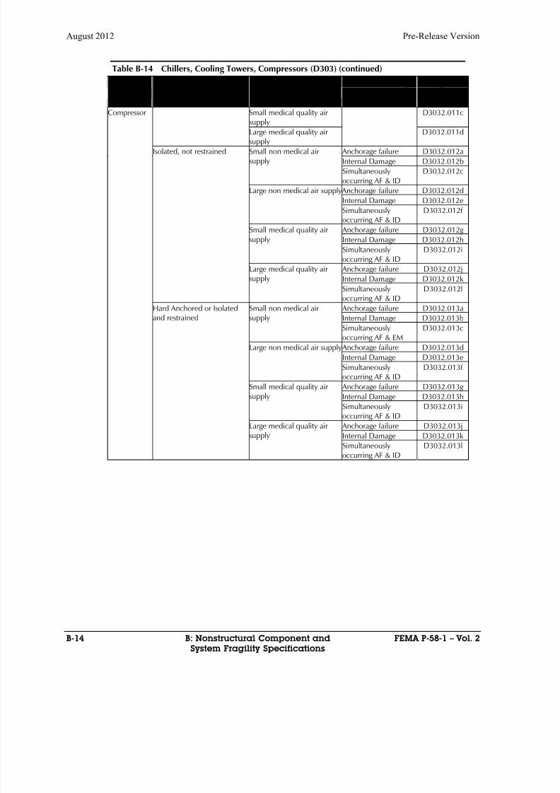
8/12/2019 Seismic Performance Assessment of Buildings
http://slidepdf.com/reader/full/seismic-performance-assessment-of-buildings 278/358
August 2012 Pre-Release Version
B-14 B: Nonstructural Component and FEMA P-58-1 – Vol. 2
System Fragility Specifications
Table B-14 Chillers, Cooling Towers, Compressors (D303) (continued)
EquipmentDescription
Installation Variables Size or Rated Capacity Dominant DamageMode
FragilityClassification
Number
Compressor Small medical quality airsupply
D3032.011c
Large medical quality airsupply
D3032.011d
Isolated, not restrained Small non medical airsupply
Anchorage failure D3032.012a
Internal Damage D3032.012b
Simultaneouslyoccurring AF & ID
D3032.012c
Large non medical air supplyAnchorage failure D3032.012d
Internal Damage D3032.012e
Simultaneouslyoccurring AF & ID
D3032.012f
Small medical quality airsupply
Anchorage failure D3032.012g
Internal Damage D3032.012h
Simultaneously
occurring AF & ID
D3032.012i
Large medical quality airsupply
Anchorage failure D3032.012j
Internal Damage D3032.012k
Simultaneouslyoccurring AF & ID
D3032.012l
Hard Anchored or Isolatedand restrained
Small non medical airsupply
Anchorage failure D3032.013a
Internal Damage D3032.013b
Simultaneouslyoccurring AF & EM
D3032.013c
Large non medical air supply
Anchorage failure D3032.013d
Internal Damage D3032.013e
Simultaneouslyoccurring AF & ID
D3032.013f
Small medical quality airsupply Anchorage failure D3032.013gInternal Damage D3032.013h
Simultaneouslyoccurring AF & ID
D3032.013i
Large medical quality airsupply
Anchorage failure D3032.013j
Internal Damage D3032.013k
Simultaneouslyoccurring AF & ID
D3032.013l
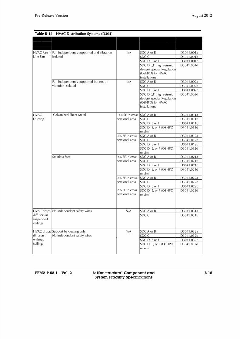
8/12/2019 Seismic Performance Assessment of Buildings
http://slidepdf.com/reader/full/seismic-performance-assessment-of-buildings 279/358
Pre-Release Version August 2012
FEMA P-58-1 – Vol. 2 B: Nonstructural Component and B-15
System Fragility Specifications
Table B-15 HVAC Distribution Systems (D304)
EquipmentDescription
Installation Variables Size, Material Seismic Rating,Dominant Damage
Mode
FragilityClassification
Number
HVAC Fan In
Line Fan
Fan independently supported and vibration
isolated
N/A SDC A or B D3041.001a
SDC C D3041.001bSDC D, E or F D3041.001c
SDC D,E,F (high seismicdesign) Special Regulation(OSHPD) for HVACinstallations
D3041.001d
Fan independently supported but not onvibration isolated
N/A SDC A or B D3041.002a
SDC C D3041.002b
SDC D, E or F D3041.002c
SDC D,E,F (high seismicdesign) Special Regulation(OSHPD) for HVACinstallations
D3041.002d
HVACDucting
Galvanized Sheet Metal <6 SF in crosssectional area
SDC A or B D3041.011a
SDC C D3041.011b
SDC D, E or F D3041.011c
SDC D, E, or F (OSHPDor sim.)
D3041.011d
≥6 SF in crosssectional area
SDC A or B D3041.012a
SDC C D3041.012b
SDC D, E or F D3041.012c
SDC D, E, or F (OSHPDor sim.)
D3041.012d
Stainless Steel <6 SF in crosssectional area
SDC A or B D3041.021a
SDC C D3041.021b
SDC D, E or F D3041.021cSDC D, E, or F (OSHPDor sim.)
D3041.021d
≥6 SF in crosssectional area
≥6 SF in crosssectional area
SDC A or B D3041.022a
SDC C D3041.022b
SDC D, E or F D3041.022c
SDC D, E, or F (OSHPDor sim.)
D3041.022d
HVAC drops/diffusers insuspended
ceilings
No independent safety wires N/A SDC A or B D3041.031a
SDC C D3041.031b
HVAC drops/diffuserswithoutceilings
Support by ducting only.No independent safety wires
N/A SDC A or B D3041.032a
SDC C D3041.032b
SDC D, E or F D3041.032c
SDC D, E, or F (OSHPDor sim.
D3041.032d

8/12/2019 Seismic Performance Assessment of Buildings
http://slidepdf.com/reader/full/seismic-performance-assessment-of-buildings 280/358
August 2012 Pre-Release Version
B-16 B: Nonstructural Component and FEMA P-58-1 – Vol. 2
System Fragility Specifications
Table B-15 HVAC Distribution Systems (D304) (continued)
EquipmentDescription
Installation Variables Size, Material Seismic Rating,Dominant Damage
Mode
FragilityClassification
Number
Variable AirVolume
(VAV) Boxwith in-linecoil
N/A N/A SDC A or B D3041.041a
SDC C D3041.041b
HVAC Fan Unanchored, not isolated N/A Internal Damage D3041.101a
Isolated, not restrained N/A Anchorage failure D3041.102a
Internal Damage D3041.102b
Simultaneously occurring AF & ID
D3041.102c
Hard anchored or isolated and restrained N/A Anchorage failure D3041.103a
Internal Damage D3041.103b
Simultaneously occurring
AF & ID
D3041.103c
Table B-16 Packaged Air Handling Unit (D305)
Equipmentdescription
Installation variables Size or rated capacity Dominant DamageMode
FragilityClassification
Number
Packaged AirHandling Unit
Unanchored, not isolated <5000 CFM Internal Damage D3052.011a
5000 to <10000 CFM D3052.011b
10000 to <25000 CFM D3052.011c
25000 to <40000 CFM D3052.011d
Hard anchored or isolatedand restrained
<5000 CFM Anchorage failure D3052.013a
Internal Damage D3052.013b
Simultaneouslyoccurring AF & ID D3052.013c
5000 to <10000 CFM Anchorage failure D3052.013d
Internal Damage D3052.013e
Simultaneouslyoccurring AF & ID
D3052.013f
10000 to <25000 CFM Anchorage failure D3052.013g
Internal Damage D3052.013h
Simultaneouslyoccurring AF & ID
D3052.013i
25000 to <40000 CFM Anchorage failure D3052.013j
Internal Damage D3052.013k
Simultaneously
occurring AF & ID
D3052.013l

8/12/2019 Seismic Performance Assessment of Buildings
http://slidepdf.com/reader/full/seismic-performance-assessment-of-buildings 281/358
Pre-Release Version August 2012
FEMA P-58-1 – Vol. 2 B: Nonstructural Component and B-17
System Fragility Specifications
Table B-17 Control Panel (D306)
Equipmentdescription
Installation variables Dominant DamageMode
FragilityClassification
Number
Control Panel Unanchored Internal Damage D3067.011a
Hard anchored Anchorage failure D3067.013a
Internal Damage D3067.013bSimultaneously occurring AF & ID
D3067.013c
Table B-18 Fire Protection (D401)
System/ItemDescription
Size Material type Installation variable FragilityClassification
Number
Fire Sprinkler WaterPiping – HorizontalMains and Branches
N/A Old StyleVictaulic, thin-wallsteel
SDC A or B D4011.021a,
SDC C D4011.022a,
SDC D, E or F D4011.023a,
SDC D, E, or F (OSHPD or
sim.)
D4011.024a,
Fire Sprinkler Drop 6 ft. longdrop max.StandardSteelThreaded
Soft lay-in tileceiling
Dropping into tile SOFTceiling, SDC A or B
D4011.031a
Dropping into lay-in tileSOFT ceiling, SDC C
D4011.032a
Dropping into lay-in tileSOFT ceiling, SDC D, E or F
D4011.033a
Dropping into lay-in tileSOFT ceiling, SDC D, E, or F(OSHPD or sim.)
D4011.034a
Hard lay-in TileCeiling
Dropping into lay-in tileHARD ceiling, SDC A or B
D4011.041a
Dropping into lay-in tileHARD ceiling, SDC C
D4011.042a
Dropping into lay-in tileHARD ceiling, SDC D, E, orF
D4011.063a
Dropping into lay-in tileHARD ceiling, SDC D, E, orF (OSHPD or sim.)
D4011.064a
No Ceiling No Ceiling, SDC A or B D4011.071a
No Ceiling, SDC C D4011.072a
No Ceiling, SDC D, E or F D4011.073a
No Ceiling, SDC D, E, or F(OSHPD or sim.)
D4011.074a
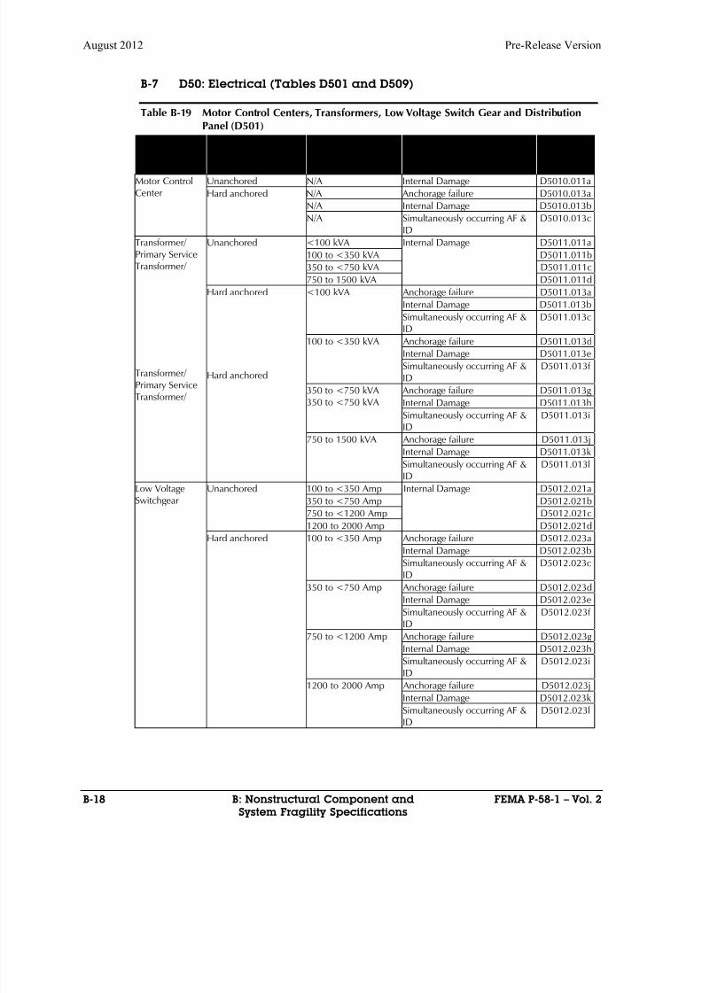
8/12/2019 Seismic Performance Assessment of Buildings
http://slidepdf.com/reader/full/seismic-performance-assessment-of-buildings 282/358
August 2012 Pre-Release Version
B-18 B: Nonstructural Component and FEMA P-58-1 – Vol. 2
System Fragility Specifications
B-7 D50: Electrical (Tables D501 and D509)
Table B-19 Motor Control Centers, Transformers, Low Voltage Switch Gear and DistributionPanel (D501)
Equipmentdescription
Installation variables Size or Rated Capacity Dominant Damage Mode FragilityClassification
Number
Motor ControlCenter
Unanchored N/A Internal Damage D5010.011a
Hard anchored N/A Anchorage failure D5010.013a
N/A Internal Damage D5010.013b
N/A Simultaneously occurring AF &ID
D5010.013c
Transformer/Primary ServiceTransformer/
Transformer/Primary ServiceTransformer/
Unanchored <100 kVA Internal Damage D5011.011a
100 to <350 kVA D5011.011b
350 to <750 kVA D5011.011c
750 to 1500 kVA D5011.011d
Hard anchored
Hard anchored
<100 kVA Anchorage failure D5011.013a
Internal Damage D5011.013b
Simultaneously occurring AF &
ID
D5011.013c
100 to <350 kVA Anchorage failure D5011.013d
Internal Damage D5011.013e
Simultaneously occurring AF &ID
D5011.013f
350 to <750 kVA350 to <750 kVA
Anchorage failure D5011.013g
Internal Damage D5011.013h
Simultaneously occurring AF &ID
D5011.013i
750 to 1500 kVA Anchorage failure D5011.013j
Internal Damage D5011.013k
Simultaneously occurring AF &ID
D5011.013l
Low VoltageSwitchgear
Unanchored 100 to <350 Amp Internal Damage D5012.021a350 to <750 Amp D5012.021b
750 to <1200 Amp D5012.021c
1200 to 2000 Amp D5012.021d
Hard anchored 100 to <350 Amp Anchorage failure D5012.023a
Internal Damage D5012.023b
Simultaneously occurring AF &ID
D5012.023c
350 to <750 Amp Anchorage failure D5012.023d
Internal Damage D5012.023e
Simultaneously occurring AF &ID
D5012.023f
750 to <1200 Amp Anchorage failure D5012.023g
Internal Damage D5012.023hSimultaneously occurring AF &ID
D5012.023i
1200 to 2000 Amp Anchorage failure D5012.023j
Internal Damage D5012.023k
Simultaneously occurring AF &ID
D5012.023l
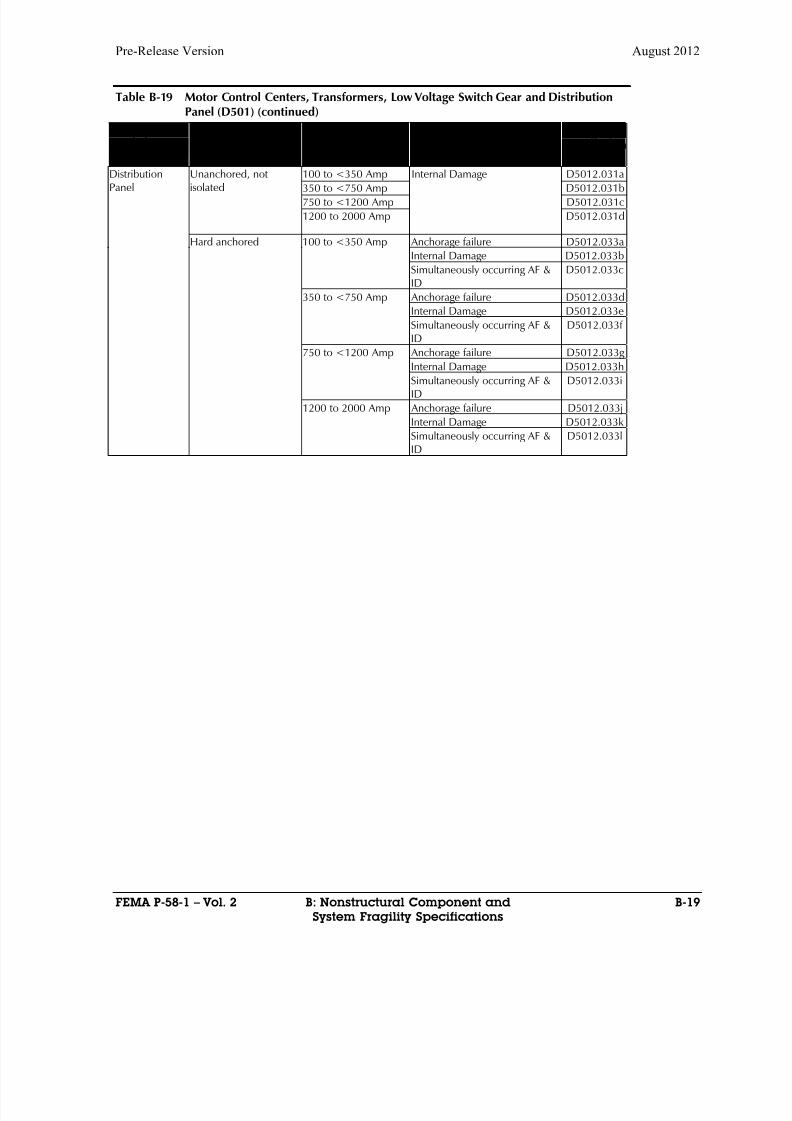
8/12/2019 Seismic Performance Assessment of Buildings
http://slidepdf.com/reader/full/seismic-performance-assessment-of-buildings 283/358
Pre-Release Version August 2012
FEMA P-58-1 – Vol. 2 B: Nonstructural Component and B-19
System Fragility Specifications
Table B-19 Motor Control Centers, Transformers, Low Voltage Switch Gear and DistributionPanel (D501) (continued)
Equipmentdescription
Installation variables Size or Rated Capacity Dominant Damage Mode FragilityClassification
Number
Distribution
Panel
Unanchored, not
isolated
100 to <350 Amp Internal Damage D5012.031a
350 to <750 Amp D5012.031b
750 to <1200 Amp D5012.031c
1200 to 2000 Amp D5012.031d
Hard anchored 100 to <350 Amp Anchorage failure D5012.033a
Internal Damage D5012.033b
Simultaneously occurring AF &ID
D5012.033c
350 to <750 Amp Anchorage failure D5012.033d
Internal Damage D5012.033e
Simultaneously occurring AF &ID
D5012.033f
750 to <1200 Amp Anchorage failure D5012.033g
Internal Damage D5012.033hSimultaneously occurring AF &ID
D5012.033i
1200 to 2000 Amp Anchorage failure D5012.033j
Internal Damage D5012.033k
Simultaneously occurring AF &ID
D5012.033l
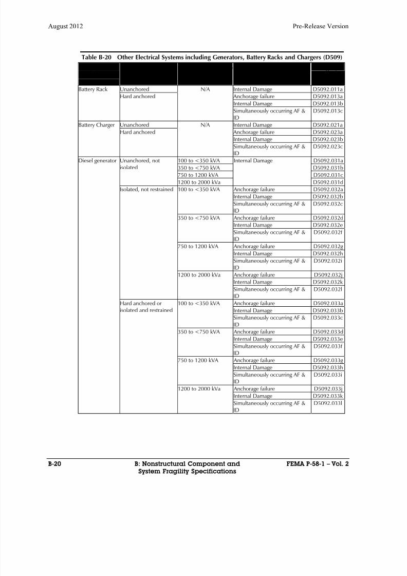
8/12/2019 Seismic Performance Assessment of Buildings
http://slidepdf.com/reader/full/seismic-performance-assessment-of-buildings 284/358
August 2012 Pre-Release Version
B-20 B: Nonstructural Component and FEMA P-58-1 – Vol. 2
System Fragility Specifications
Table B-20 Other Electrical Systems including Generators, Battery Racks and Chargers (D509)
Equipmentdescription
Installation variables Size or Rated Capacity Dominant Damage Mode FragilityClassification
Number
Battery Rack Unanchored N/A Internal Damage D5092.011a
Hard anchored Anchorage failure D5092.013aInternal Damage D5092.013b
Simultaneously occurring AF &ID
D5092.013c
Battery Charger Unanchored N/A Internal Damage D5092.021a
Hard anchored Anchorage failure D5092.023a
Internal Damage D5092.023b
Simultaneously occurring AF &ID
D5092.023c
Diesel generator Unanchored, notisolated
100 to <350 kVA Internal Damage D5092.031a
350 to <750 kVA D5092.031b
750 to 1200 kVA D5092.031c
1200 to 2000 kVa D5092.031d
Isolated, not restrained 100 to <350 kVA Anchorage failure D5092.032aInternal Damage D5092.032b
Simultaneously occurring AF &ID
D5092.032c
350 to <750 kVA Anchorage failure D5092.032d
Internal Damage D5092.032e
Simultaneously occurring AF &ID
D5092.032f
750 to 1200 kVA Anchorage failure D5092.032g
Internal Damage D5092.032h
Simultaneously occurring AF &ID
D5092.032i
1200 to 2000 kVa Anchorage failure D5092.032j
Internal Damage D5092.032kSimultaneously occurring AF &ID
D5092.032l
Hard anchored orisolated and restrained
100 to <350 kVA Anchorage failure D5092.033a
Internal Damage D5092.033b
Simultaneously occurring AF &ID
D5092.033c
350 to <750 kVA Anchorage failure D5092.033d
Internal Damage D5092.033e
Simultaneously occurring AF &ID
D5092.033f
750 to 1200 kVA Anchorage failure D5092.033g
Internal Damage D5092.033h
Simultaneously occurring AF &ID D5092.033i
1200 to 2000 kVa Anchorage failure D5092.033j
Internal Damage D5092.033k
Simultaneously occurring AF &ID
D5092.033l
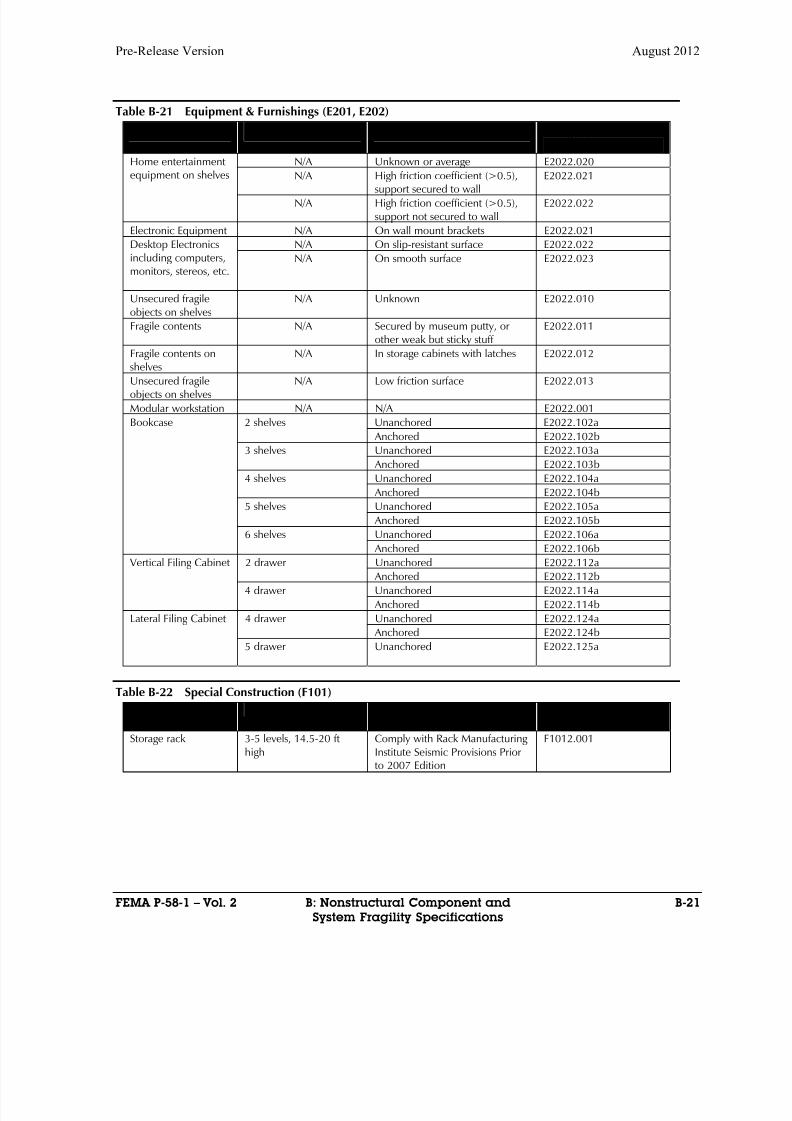
8/12/2019 Seismic Performance Assessment of Buildings
http://slidepdf.com/reader/full/seismic-performance-assessment-of-buildings 285/358
Pre-Release Version August 2012
FEMA P-58-1 – Vol. 2 B: Nonstructural Component and B-21
System Fragility Specifications
Table B-21 Equipment & Furnishings (E201, E202)
Item Description Size Seismic Installation Condition Fragility ClassificationNumber
Home entertainmentequipment on shelves
N/A Unknown or average E2022.020
N/A High friction coefficient (>0.5),support secured to wall
E2022.021
N/A High friction coefficient (>0.5),support not secured to wall
E2022.022
Electronic Equipment N/A On wall mount brackets E2022.021
Desktop Electronicsincluding computers,monitors, stereos, etc.
N/A On slip-resistant surface E2022.022
N/A On smooth surface E2022.023
Unsecured fragileobjects on shelves
N/A Unknown E2022.010
Fragile contents N/A Secured by museum putty, orother weak but sticky stuff
E2022.011
Fragile contents on
shelves
N/A In storage cabinets with latches E2022.012
Unsecured fragileobjects on shelves
N/A Low friction surface E2022.013
Modular workstation N/A N/A E2022.001
Bookcase 2 shelves Unanchored E2022.102a
Anchored E2022.102b
3 shelves Unanchored E2022.103a
Anchored E2022.103b
4 shelves Unanchored E2022.104a
Anchored E2022.104b
5 shelves Unanchored E2022.105a
Anchored E2022.105b
6 shelves Unanchored E2022.106a
Anchored E2022.106bVertical Filing Cabinet 2 drawer Unanchored E2022.112a
Anchored E2022.112b
4 drawer Unanchored E2022.114a
Anchored E2022.114b
Lateral Filing Cabinet 4 drawer Unanchored E2022.124a
Anchored E2022.124b
5 drawer Unanchored E2022.125a
Table B-22 Special Construction (F101)
Item Description Size Seismic Installation Condition Fragility ClassificationNumber
Storage rack 3-5 levels, 14.5-20 fthigh
Comply with Rack ManufacturingInstitute Seismic Provisions Priorto 2007 Edition
F1012.001

8/12/2019 Seismic Performance Assessment of Buildings
http://slidepdf.com/reader/full/seismic-performance-assessment-of-buildings 286/358
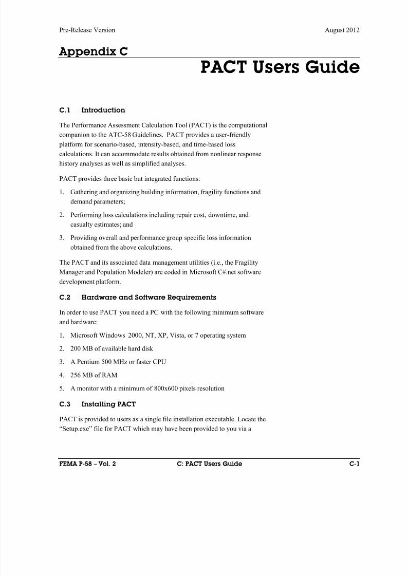
8/12/2019 Seismic Performance Assessment of Buildings
http://slidepdf.com/reader/full/seismic-performance-assessment-of-buildings 287/358
Pre-Release Version August 2012
FEMA P-58 – Vol. 2 C: PACT Users Guide C-1
Appendix C
PACT Users Guide
C.1 Introduction
The Performance Assessment Calculation Tool (PACT) is the computational
companion to the ATC-58 Guidelines. PACT provides a user-friendly
platform for scenario-based, intensity-based, and time-based loss
calculations. It can accommodate results obtained from nonlinear response
history analyses as well as simplified analyses.
PACT provides three basic but integrated functions:
1. Gathering and organizing building information, fragility functions and
demand parameters;
2. Performing loss calculations including repair cost, downtime, and
casualty estimates; and
3. Providing overall and performance group specific loss information
obtained from the above calculations.
The PACT and its associated data management utilities (i.e., the Fragility
Manager and Population Modeler) are coded in Microsoft C#.net software
development platform.
C.2 Hardware and Software Requirements
In order to use PACT you need a PC with the following minimum software
and hardware:
1. Microsoft Windows 2000, NT, XP, Vista, or 7 operating system
2. 200 MB of available hard disk
3. A Pentium 500 MHz or faster CPU
4.
256 MB of RAM
5. A monitor with a minimum of 800x600 pixels resolution
C.3 Installing PACT
PACT is provided to users as a single file installation executable. Locate the
“Setup.exe” file for PACT which may have been provided to you via a
8/12/2019 Seismic Performance Assessment of Buildings
http://slidepdf.com/reader/full/seismic-performance-assessment-of-buildings 288/358
August 2012 Pre-Release Version
C-2 C: PACT Users Guide FEMA P-58 – Vol. 2
website, an FTP download site or on a CD and double-click it. The Setup
program will guide you through the installation.
PACT requires the free Microsoft Net Framework 3.5 to be installed on your
PC. Most newer computers have this utility installed as a part of their
operating system. The PACT installer checks your computer for presence ofthe Microsoft Net Framework 3.5 and if necessary it will download and
install it for you from the Microsoft website. Therefore, it is prudent that you
establish Internet connectivity during the PACT installation process.
Once the installation is completed, a shortcut to PACT is placed on your
desktop that you can use to access the program.
Figure C-1 PACT shortcut.
C.4 What is new in PACT?
C.4.1 General
PACT provides the capability of modeling repair time (downtime) and
casualties (death and injuries), unsafe placard probabilities, residual drift,
and structural collapse probabilities and consequences. The previous
version of PACT was developed in Microsoft Visual Basic programming
language.
PACT is completely re-written using object oriented paradigms for easier
readability, maintenance, and upgradability in Microsoft Visual Studio
2010 in C#.net.
The code size is more than double that of previous version of PACT.
Only one commercial third party control is used (for creating graphs) and
PACT users do not need to license any software or utilities in order to
use PACT. Those who want to modify the code or further develop PACT
need to license only one third party control.
PACT code is split into logical units, allowing separation of the FragilityManager, Population Manager, Building Manager, Core Engine,
Reporting, and Result Viewer into standalone units.
PACT is unit independent and Imperial as well as S.I. units are
accommodated.
8/12/2019 Seismic Performance Assessment of Buildings
http://slidepdf.com/reader/full/seismic-performance-assessment-of-buildings 289/358
Pre-Release Version August 2012
FEMA P-58 – Vol. 2 C: PACT Users Guide C-3
C.4.2 Fragilities
Ability to customize and add new demand parameters
Implementation of fragility ratings
Ability to add additional notes, comments, and author information
Inclusion of sequential, mutually exclusive, and simultaneous damage
states
Implementation of sub-damage states, including almost any combination
of the above damage states in any order
Implementation of repair time (downtime) consequences
Ability to choose normal or lognormal distributions for cost and
downtime consequences
Implementation of unsafe placard consequences
Implementation of non-collapse death and injury consequences
Ability to identify and track items with long lead time consequences
C.4.3 Building Manager
Implementation of region and date cost adjustment multipliers
Implementation of height, hazmat, and occupancy multipliers on a floor-
by-floor basis
Building collapse specifications, including different modes, floor
percentages, and death and injury rate consequences
Implementation of user-defined (custom) demand parameters (EDP
types).
Replacement cost and total loss threshold cutoffs
Repair time (downtime) calculations using serial and parallel repair
strategies.
Maximum workers per unit of area measurement
Quantity uncertainty for performance groups
The ability to set damage correlation per performance group
Ability to assign multiple occupancies, population models, structural
systems and combination on each floor and throughout the building.
Implementation of unrepairable residual drift
8/12/2019 Seismic Performance Assessment of Buildings
http://slidepdf.com/reader/full/seismic-performance-assessment-of-buildings 290/358
August 2012 Pre-Release Version
C-4 C: PACT Users Guide FEMA P-58 – Vol. 2
C.4.4 Evaluate Performance
Completely reworked integration algorithms
Parallel processing on multi-core computers to reduce execution time
User can select a project-wide random seed value for consistent results
Implementation of a variety of runtime progress indicators
Command line version for automated runs
C.4.5 Viewing Results
New graphs to show the new types of data developed for PACT.
New ways of manipulating the already existing types of graphs
Brand new types of graphs, showing different ways of examining the
results
A wide variety of data export options
The ability to drill down on the data, from the entire building all the way
down to individual realizations, performance groups, and performance
group items.
The ability to save and load the result files.
Automatic generation of reports in Microsoft Word format
C.5 Using PACT
C.5.1 PACT Control Panel
Once you start PACT the Pact Control Panel appears. The PACT Control
Panel is the focal point of your activities when you use the program. You will
come back to this panel before and after completion of each major task.
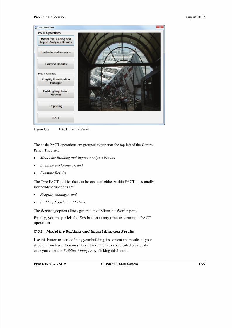
8/12/2019 Seismic Performance Assessment of Buildings
http://slidepdf.com/reader/full/seismic-performance-assessment-of-buildings 291/358
Pre-Release Version August 2012
FEMA P-58 – Vol. 2 C: PACT Users Guide C-5
Figure C-2 PACT Control Panel.
The basic PACT operations are grouped together at the top left of the Control
Panel. They are:
Model the Building and Import Analyses Results
Evaluate Performance, and
Examine Results
The Two PACT utilities that can be operated either within PACT or as totally
independent functions are:
Fragility Manager, and
Building Population Modeler
The Reporting option allows generation of Microsoft Word reports.
Finally, you may click the Exit button at any time to terminate PACToperation.
C.5.2 Model the Building and Import Analyses Results
Use this button to start defining your building, its content and results of your
structural analyses. You may also retrieve the files you created previously
once you enter the Building Manager by clicking this button.
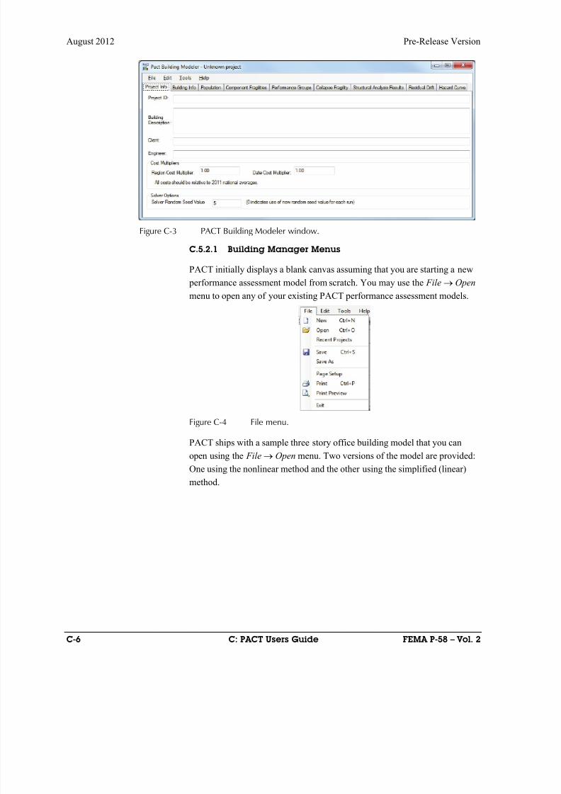
8/12/2019 Seismic Performance Assessment of Buildings
http://slidepdf.com/reader/full/seismic-performance-assessment-of-buildings 292/358
August 2012 Pre-Release Version
C-6 C: PACT Users Guide FEMA P-58 – Vol. 2
Figure C-3 PACT Building Modeler window.
C.5.2.1 Building Manager Menus
PACT initially displays a blank canvas assuming that you are starting a new
performance assessment model from scratch. You may use the File Open
menu to open any of your existing PACT performance assessment models.
Figure C-4 File menu.
PACT ships with a sample three story office building model that you can
open using the File Open menu. Two versions of the model are provided:
One using the nonlinear method and the other using the simplified (linear)
method.

8/12/2019 Seismic Performance Assessment of Buildings
http://slidepdf.com/reader/full/seismic-performance-assessment-of-buildings 293/358
Pre-Release Version August 2012
FEMA P-58 – Vol. 2 C: PACT Users Guide C-7
Figure C-5 Open File menu.
Once an existing PACT file is opened, the blank fields are overwritten by the
relevant information contained in the opened file.
Figure C-6 PACT Building Modeler with retrieved data from opened file.
Under the File Menu, besides Open you can use New to start a new project
from scratch, Recent Projects to see a list of projects you have worked on
recently, Save to save the project under its current name, Save As to save a
copy of the project under a new name. In addition, you can use Page Setup to
setup your printer and your print preferences, Print to print a copy of the
form displayed on your screen and Print Review to take a look at how such a
printout would look like. Finally, you can click Exit to leave the building
manager and return to the control panel.
Under the Edit Menu, you can use Cut , Copy, Paste, and Select All to cut and
past the contents of one or several cells. This becomes handy when you want
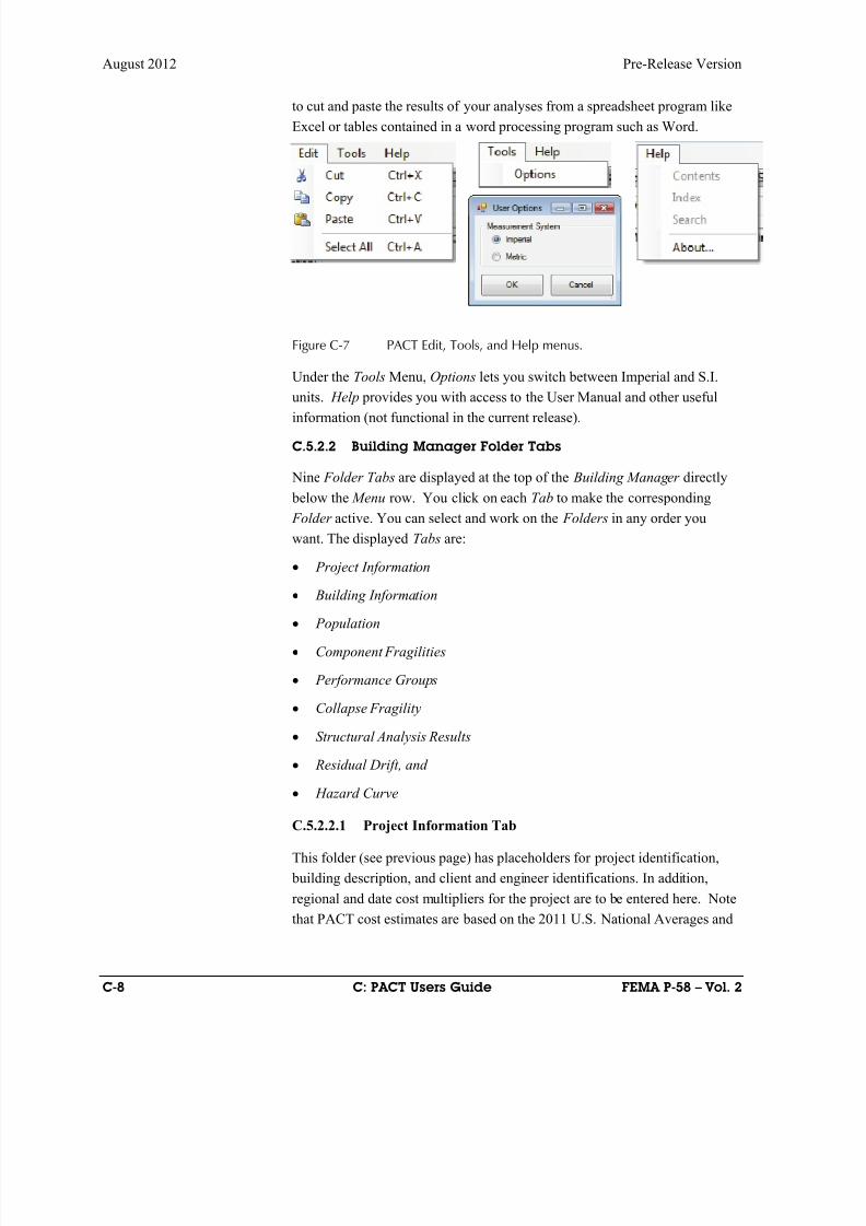
8/12/2019 Seismic Performance Assessment of Buildings
http://slidepdf.com/reader/full/seismic-performance-assessment-of-buildings 294/358
August 2012 Pre-Release Version
C-8 C: PACT Users Guide FEMA P-58 – Vol. 2
to cut and paste the results of your analyses from a spreadsheet program like
Excel or tables contained in a word processing program such as Word.
Figure C-7 PACT Edit, Tools, and Help menus.
Under the Tools Menu, Options lets you switch between Imperial and S.I.
units. Help provides you with access to the User Manual and other usefulinformation (not functional in the current release).
C.5.2.2 Building Manager Folder Tabs
Nine Folder Tabs are displayed at the top of the Building Manager directly
below the Menu row. You click on each Tab to make the corresponding
Folder active. You can select and work on the Folders in any order you
want. The displayed Tabs are:
Project Information
Building Information
Population
Component Fragilities
Performance Groups
Collapse Fragility
Structural Analysis Results
Residual Drift, and
Hazard Curve
C.5.2.2.1 Project Information Tab
This folder (see previous page) has placeholders for project identification,
building description, and client and engineer identifications. In addition,
regional and date cost multipliers for the project are to be entered here. Note
that PACT cost estimates are based on the 2011 U.S. National Averages and
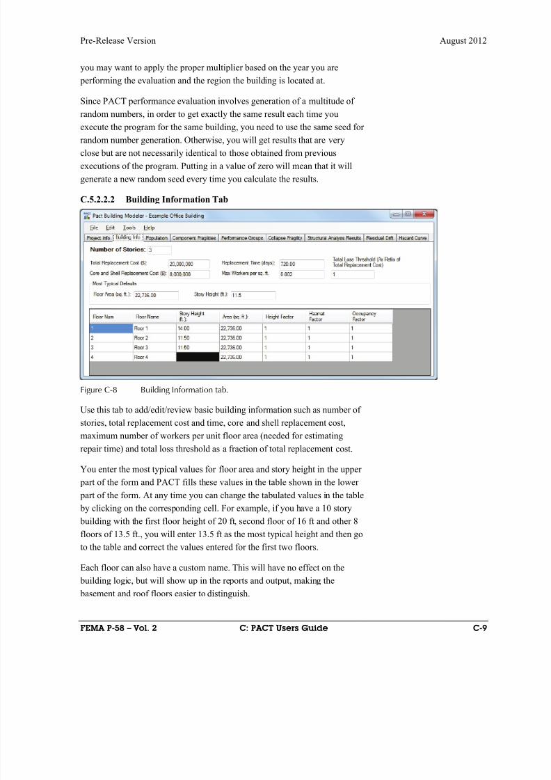
8/12/2019 Seismic Performance Assessment of Buildings
http://slidepdf.com/reader/full/seismic-performance-assessment-of-buildings 295/358
Pre-Release Version August 2012
FEMA P-58 – Vol. 2 C: PACT Users Guide C-9
you may want to apply the proper multiplier based on the year you are
performing the evaluation and the region the building is located at.
Since PACT performance evaluation involves generation of a multitude of
random numbers, in order to get exactly the same result each time you
execute the program for the same building, you need to use the same seed forrandom number generation. Otherwise, you will get results that are very
close but are not necessarily identical to those obtained from previous
executions of the program. Putting in a value of zero will mean that it will
generate a new random seed every time you calculate the results.
C.5.2.2.2 Building Information Tab
Figure C-8 Building Information tab.
Use this tab to add/edit/review basic building information such as number of
stories, total replacement cost and time, core and shell replacement cost,
maximum number of workers per unit floor area (needed for estimating
repair time) and total loss threshold as a fraction of total replacement cost.
You enter the most typical values for floor area and story height in the upper
part of the form and PACT fills these values in the table shown in the lower
part of the form. At any time you can change the tabulated values in the table
by clicking on the corresponding cell. For example, if you have a 10 story building with the first floor height of 20 ft, second floor of 16 ft and other 8
floors of 13.5 ft., you will enter 13.5 ft as the most typical height and then go
to the table and correct the values entered for the first two floors.
Each floor can also have a custom name. This will have no effect on the
building logic, but will show up in the reports and output, making the
basement and roof floors easier to distinguish.
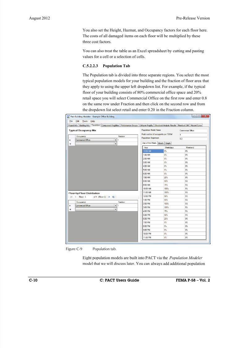
8/12/2019 Seismic Performance Assessment of Buildings
http://slidepdf.com/reader/full/seismic-performance-assessment-of-buildings 296/358
August 2012 Pre-Release Version
C-10 C: PACT Users Guide FEMA P-58 – Vol. 2
You also set the Height, Hazmat, and Occupancy factors for each floor here.
The costs of all damaged items on each floor will be multiplied by these
three cost factors.
You can also treat the table as an Excel spreadsheet by cutting and pasting
values for a cell or a selection of cells.
C.5.2.2.3 Population Tab
The Population tab is divided into three separate regions. You select the most
typical population models for your building and the fraction of floor area that
they apply to using the upper left dropdown list. For example, if the typical
floor of your building consists of 80% commercial office space and 20%
retail space you will select Commercial Office on the first row and enter 0.8
on the same row under Fraction and then click on the second row and from
the dropdown list select retail and enter 0.20 in the Fraction column.
Figure C-9 Population tab.
Eight population models are built into PACT via the Population Modeler
model that we will discuss later. You can always add additional population
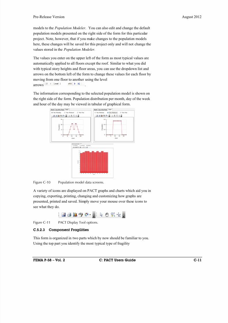
8/12/2019 Seismic Performance Assessment of Buildings
http://slidepdf.com/reader/full/seismic-performance-assessment-of-buildings 297/358
Pre-Release Version August 2012
FEMA P-58 – Vol. 2 C: PACT Users Guide C-11
models to the Population Modeler. You can also edit and change the default
population models presented on the right side of the form for this particular
project. Note, however, that if you make changes to the population models
here, these changes will be saved for this project only and will not change the
values stored in the Population Modeler.
The values you enter on the upper left of the form as most typical values are
automatically applied to all floors except the roof. Similar to what you did
with typical story heights and floor areas, you can use the dropdown list and
arrows on the bottom left of the form to change these values for each floor by
moving from one floor to another using the level
arrows .
The information corresponding to the selected population model is shown on
the right side of the form. Population distribution per month, day of the week
and hour of the day may be viewed in tabular of graphical form.
Figure C-10 Population model data screens.
A variety of icons are displayed on PACT graphs and charts which aid you in
copying, exporting, printing, changing and customizing how graphs are
presented, printed and saved. Simply move your mouse over these icons to
see what they do.
Figure C-11 PACT Display Tool options.
C.5.2.3 Component Fragilities
This form is organized in two parts which by now should be familiar to you.
Using the top part you identify the most typical type of fragility
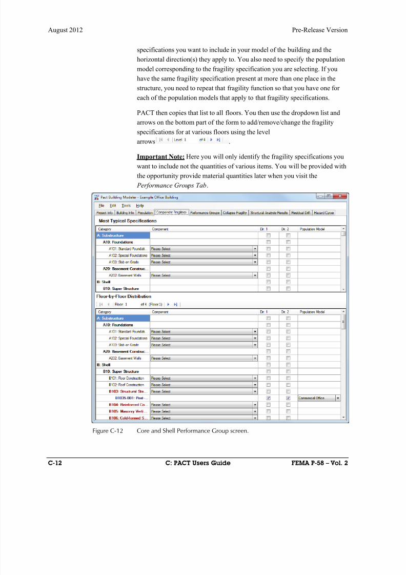
8/12/2019 Seismic Performance Assessment of Buildings
http://slidepdf.com/reader/full/seismic-performance-assessment-of-buildings 298/358
August 2012 Pre-Release Version
C-12 C: PACT Users Guide FEMA P-58 – Vol. 2
specifications you want to include in your model of the building and the
horizontal direction(s) they apply to. You also need to specify the population
model corresponding to the fragility specification you are selecting. If you
have the same fragility specification present at more than one place in the
structure, you need to repeat that fragility function so that you have one for
each of the population models that apply to that fragility specifications.
PACT then copies that list to all floors. You then use the dropdown list and
arrows on the bottom part of the form to add/remove/change the fragility
specifications for at various floors using the level
arrows .
Important Note: Here you will only identify the fragility specifications you
want to include not the quantities of various items. You will be provided with
the opportunity provide material quantities later when you visit the
Performance Groups Tab.
Figure C-12 Core and Shell Performance Group screen.

8/12/2019 Seismic Performance Assessment of Buildings
http://slidepdf.com/reader/full/seismic-performance-assessment-of-buildings 299/358
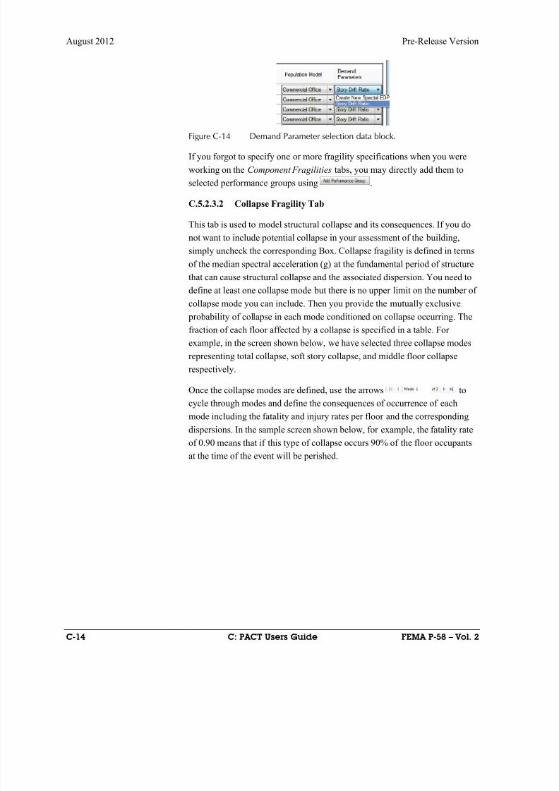
8/12/2019 Seismic Performance Assessment of Buildings
http://slidepdf.com/reader/full/seismic-performance-assessment-of-buildings 300/358
August 2012 Pre-Release Version
C-14 C: PACT Users Guide FEMA P-58 – Vol. 2
Figure C-14 Demand Parameter selection data block.
If you forgot to specify one or more fragility specifications when you were
working on the Component Fragilities tabs, you may directly add them to
selected performance groups using .
C.5.2.3.2 Collapse Fragility Tab
This tab is used to model structural collapse and its consequences. If you do
not want to include potential collapse in your assessment of the building,
simply uncheck the corresponding Box. Collapse fragility is defined in terms
of the median spectral acceleration (g) at the fundamental period of structure
that can cause structural collapse and the associated dispersion. You need to
define at least one collapse mode but there is no upper limit on the number of
collapse mode you can include. Then you provide the mutually exclusive
probability of collapse in each mode conditioned on collapse occurring. The
fraction of each floor affected by a collapse is specified in a table. For
example, in the screen shown below, we have selected three collapse modes
representing total collapse, soft story collapse, and middle floor collapse
respectively.
Once the collapse modes are defined, use the arrows tocycle through modes and define the consequences of occurrence of each
mode including the fatality and injury rates per floor and the corresponding
dispersions. In the sample screen shown below, for example, the fatality rate
of 0.90 means that if this type of collapse occurs 90% of the floor occupants
at the time of the event will be perished.
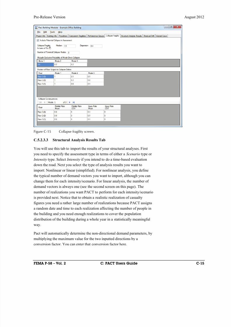
8/12/2019 Seismic Performance Assessment of Buildings
http://slidepdf.com/reader/full/seismic-performance-assessment-of-buildings 301/358
Pre-Release Version August 2012
FEMA P-58 – Vol. 2 C: PACT Users Guide C-15
Figure C-15 Collapse fragility screen.
C.5.2.3.3 Structural Analysis Results Tab
You will use this tab to import the results of your structural analyses. First
you need to specify the assessment type in terms of either a Scenario type or
Intensity type. Select Intensity if you intend to do a time-based evaluationdown the road. Next you select the type of analysis results you want to
import: Nonlinear or linear (simplified). For nonlinear analysis, you define
the typical number of demand vectors you want to import, although you can
change them for each intensity/scenario. For linear analysis, the number of
demand vectors is always one (see the second screen on this page). The
number of realizations you want PACT to perform for each intensity/scenario
is provided next. Notice that to obtain a realistic realization of casualty
figures you need a rather large number of realizations because PACT assigns
a random date and time to each realization affecting the number of people in
the building and you need enough realizations to cover the populationdistribution of the building during a whole year in a statistically meaningful
way.
Pact will automatically determine the non-directional demand parameters, by
multiplying the maximum value for the two inputted directions by a
conversion factor. You can enter that conversion factor here.
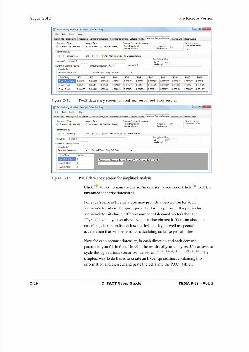
8/12/2019 Seismic Performance Assessment of Buildings
http://slidepdf.com/reader/full/seismic-performance-assessment-of-buildings 302/358
August 2012 Pre-Release Version
C-16 C: PACT Users Guide FEMA P-58 – Vol. 2
Figure C-16 PACT data entry screen for nonlinear response-history results.
Figure C-17 PACT data entry screen for simplified analysis.
Click to add as many scenarios/intensities as you need. Click to delete
unwanted scenarios/intensities.
For each Scenario/Intensity you may provide a description for each
scenario/intensity in the space provided for this purpose. If a particular
scenario/intensity has a different number of demand vectors than the
“Typical” value you set above, you can also change it. You can also set a
modeling dispersion for each scenario/intensity, as well as spectral
acceleration that will be used for calculating collapse probabilities.
Now for each scenario/intensity, in each direction and each demand
parameter you fill in the table with the results of your analyses. Use arrows to
cycle through various scenarios/intensities . The
simplest way to do this is to create an Excel spreadsheet containing this
information and then cut and paste the cells into the PACT tables.
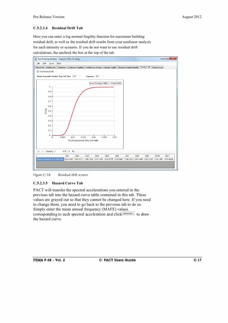
8/12/2019 Seismic Performance Assessment of Buildings
http://slidepdf.com/reader/full/seismic-performance-assessment-of-buildings 303/358
Pre-Release Version August 2012
FEMA P-58 – Vol. 2 C: PACT Users Guide C-17
C.5.2.3.4 Residual Drift Tab
Here you can enter a log-normal fragility function for maximum building
residual drift, as well as the residual drift results from your nonlinear analysis
for each intensity or scenario. If you do not want to use residual drift
calculations, the uncheck the box at the top of the tab.
Figure C-18 Residual drift screen.
C.5.2.3.5 Hazard Curve Tab
PACT will transfer the spectral accelerations you entered in the
previous tab into the hazard curve table contained in this tab. These
values are grayed out so that they cannot be changed here. If you need
to change them, you need to go back to the previous tab to do so.Simply enter the mean annual frequency (MAFE) values
corresponding to each spectral acceleration and click to drawthe hazard curve.
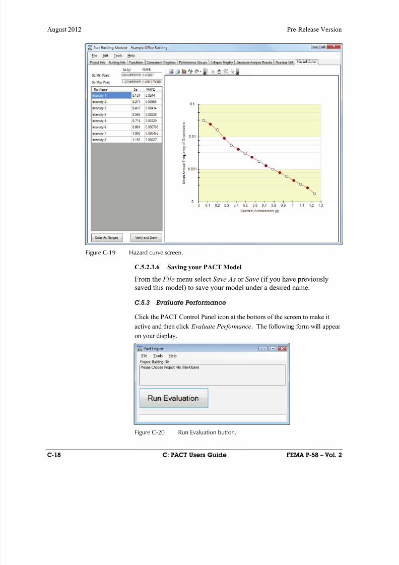
8/12/2019 Seismic Performance Assessment of Buildings
http://slidepdf.com/reader/full/seismic-performance-assessment-of-buildings 304/358
August 2012 Pre-Release Version
C-18 C: PACT Users Guide FEMA P-58 – Vol. 2
Figure C-19 Hazard curve screen.
C.5.2.3.6 Saving your PACT Model
From the File menu select Save As or Save (if you have previouslysaved this model) to save your model under a desired name.
C.5.3 Evaluate Performance
Click the PACT Control Panel icon at the bottom of the screen to make it
active and then click Evaluate Performance. The following form will appear
on your display.
Figure C-20 Run Evaluation button.
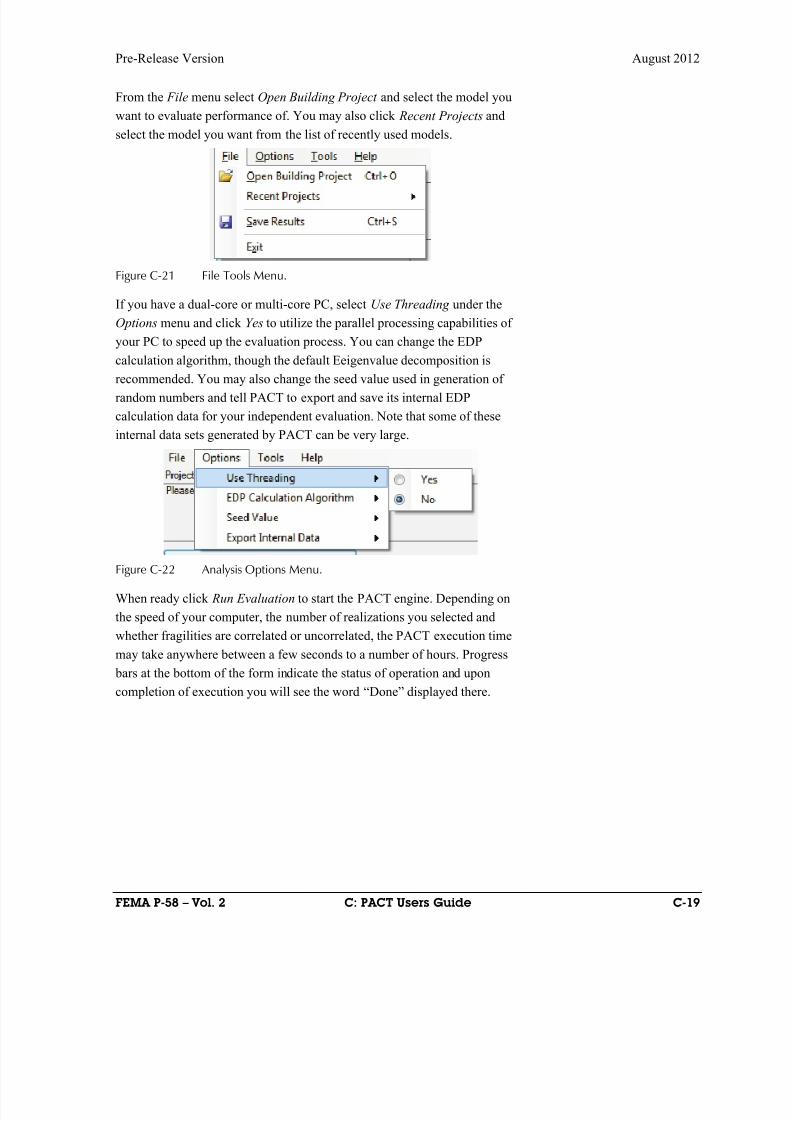
8/12/2019 Seismic Performance Assessment of Buildings
http://slidepdf.com/reader/full/seismic-performance-assessment-of-buildings 305/358
Pre-Release Version August 2012
FEMA P-58 – Vol. 2 C: PACT Users Guide C-19
From the File menu select Open Building Project and select the model you
want to evaluate performance of. You may also click Recent Projects and
select the model you want from the list of recently used models.
Figure C-21 File Tools Menu.
If you have a dual-core or multi-core PC, select Use Threading under the
Options menu and click Yes to utilize the parallel processing capabilities of
your PC to speed up the evaluation process. You can change the EDP
calculation algorithm, though the default Eeigenvalue decomposition is
recommended. You may also change the seed value used in generation of
random numbers and tell PACT to export and save its internal EDP
calculation data for your independent evaluation. Note that some of these
internal data sets generated by PACT can be very large.
Figure C-22 Analysis Options Menu.
When ready click Run Evaluation to start the PACT engine. Depending on
the speed of your computer, the number of realizations you selected and
whether fragilities are correlated or uncorrelated, the PACT execution time
may take anywhere between a few seconds to a number of hours. Progress
bars at the bottom of the form indicate the status of operation and upon
completion of execution you will see the word “Done” displayed there.
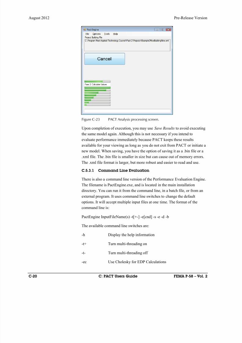
8/12/2019 Seismic Performance Assessment of Buildings
http://slidepdf.com/reader/full/seismic-performance-assessment-of-buildings 306/358
August 2012 Pre-Release Version
C-20 C: PACT Users Guide FEMA P-58 – Vol. 2
Figure C-23 PACT Analysis processing screen.
Upon completion of execution, you may use Save Results to avoid executing
the same model again. Although this is not necessary if you intend to
evaluate performance immediately because PACT keeps these results
available for your viewing as long as you do not exit from PACT or initiate a
new model. When saving, you have the option of saving it as a .bin file or a
.xml file. The .bin file is smaller in size but can cause out of memory errors.
The .xml file format is larger, but more robust and easier to read and use.
C.5.3.1 Command Line Evaluation
There is also a command line version of the Performance Evaluation Engine.
The filename is PactEngine.exe, and is located in the main installation
directory. You can run it from the command line, in a batch file, or from an
external program. It uses command line switches to change the default
options. It will accept multiple input files at one time. The format of the
command line is:
PactEngine InputFileName(s) -t[+-] -e[cnd] -s -e -d -b
The available command line switches are:
-h Display the help information
-t+ Turn multi-threading on
-t- Turn multi-threading off
-ec Use Cholesky for EDP Calculations

8/12/2019 Seismic Performance Assessment of Buildings
http://slidepdf.com/reader/full/seismic-performance-assessment-of-buildings 307/358
Pre-Release Version August 2012
FEMA P-58 – Vol. 2 C: PACT Users Guide C-21
-en Use a Normal Distribution for EDP Calculations
-ed Use Eigenvalue Decomposition for EDP Calculations
-s # Override the seed value
-e Export Internal Data
-d Add Date/Time stamp to output filename
-b Save results as a binary formatted file (default is XML
format)
The output file will be saved in the same directory as the input file, with the
default name of inputFileName_results.xml, unless the -d option is selected,
where it will add the date/time stamp of the analysis to the run, in which case
the format will be InputFileName_results_YYYY-MM-DDTHH.MM.SS.xml
(e.g. InputFileName_results_2011-12-31T14.30.00.xml is Dec 31, 2011, at2:30 in the afternoon).
If a particular command line switch is not used it will use the default option
last selected when using the GUI, unless otherwise specified above.
C.5.4 Examine Results
Click the PACT Control Panel icon at the bottom of the screen to make it
active and then click Examine Results.
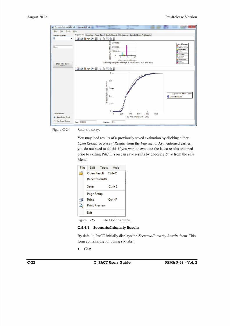
8/12/2019 Seismic Performance Assessment of Buildings
http://slidepdf.com/reader/full/seismic-performance-assessment-of-buildings 308/358
August 2012 Pre-Release Version
C-22 C: PACT Users Guide FEMA P-58 – Vol. 2
Figure C-24 Results display.
You may load results of a previously saved evaluation by clicking either
Open Results or Recent Results from the File menu. As mentioned earlier,
you do not need to do this if you want to evaluate the latest results obtained
prior to exiting PACT. You can save results by choosing Save from the File
Menu.
Figure C-25 File Options menu.
C.5.4.1 Scenario/Intensity Results
By default, PACT initially displays the Scenario/Intensity Results form. This
form contains the following six tabs:
Cost
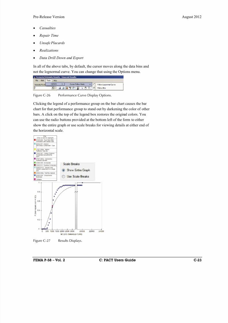
8/12/2019 Seismic Performance Assessment of Buildings
http://slidepdf.com/reader/full/seismic-performance-assessment-of-buildings 309/358
Pre-Release Version August 2012
FEMA P-58 – Vol. 2 C: PACT Users Guide C-23
Casualties
Repair Time
Unsafe Placards
Realizations
Data Drill Down and Export
In all of the above tabs, by default, the cursor moves along the data bins and
not the lognormal curve. You can change that using the Options menu.
Figure C-26 Performance Curve Display Options.
Clicking the legend of a performance group on the bar chart causes the bar
chart for that performance group to stand out by darkening the color of other
bars. A click on the top of the legend box restores the original colors. You
can use the radio buttons provided at the bottom left of the form to either
show the entire graph or use scale breaks for viewing details at either end of
the horizontal scale.
Figure C-27 Results Displays.
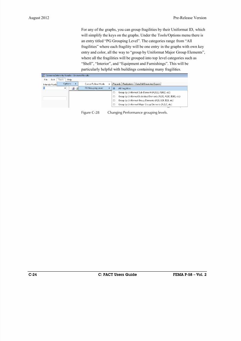
8/12/2019 Seismic Performance Assessment of Buildings
http://slidepdf.com/reader/full/seismic-performance-assessment-of-buildings 310/358
August 2012 Pre-Release Version
C-24 C: PACT Users Guide FEMA P-58 – Vol. 2
For any of the graphs, you can group fragilities by their Uniformat ID, which
will simplify the keys on the graphs. Under the Tools/Options menu there is
an entry titled “PG Grouping Level”. The categories range from “All
fragilities” where each fragility will be one entry in the graphs with own key
entry and color, all the way to “group by Uniformat Major Group Elements”,
where all the fragilities will be grouped into top level categories such as
“Shell”, “Interior”, and “Equipment and Furnishings”. This will be
particularly helpful with buildings containing many fragilities.
Figure C-28 Changing Performance grouping levels.
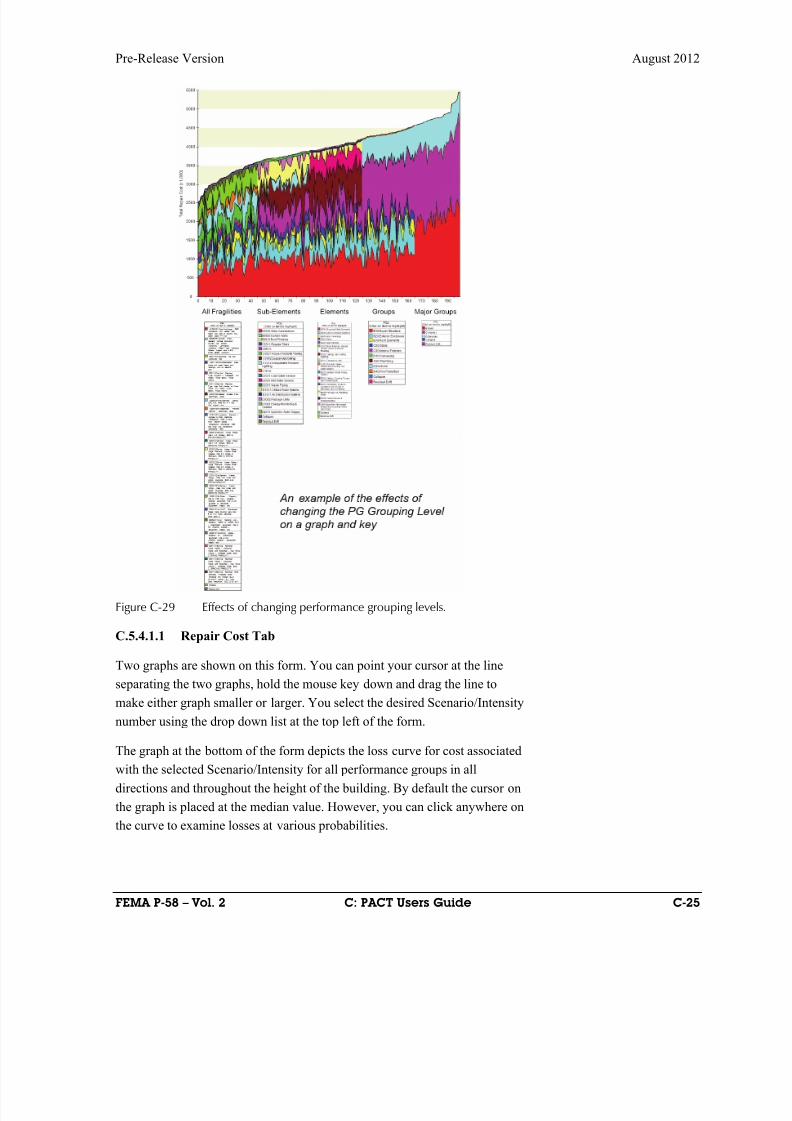
8/12/2019 Seismic Performance Assessment of Buildings
http://slidepdf.com/reader/full/seismic-performance-assessment-of-buildings 311/358
Pre-Release Version August 2012
FEMA P-58 – Vol. 2 C: PACT Users Guide C-25
Figure C-29 Effects of changing performance grouping levels.
C.5.4.1.1 Repair Cost Tab
Two graphs are shown on this form. You can point your cursor at the line
separating the two graphs, hold the mouse key down and drag the line to
make either graph smaller or larger. You select the desired Scenario/Intensity
number using the drop down list at the top left of the form.
The graph at the bottom of the form depicts the loss curve for cost associated
with the selected Scenario/Intensity for all performance groups in all
directions and throughout the height of the building. By default the cursor on
the graph is placed at the median value. However, you can click anywhere on
the curve to examine losses at various probabilities.
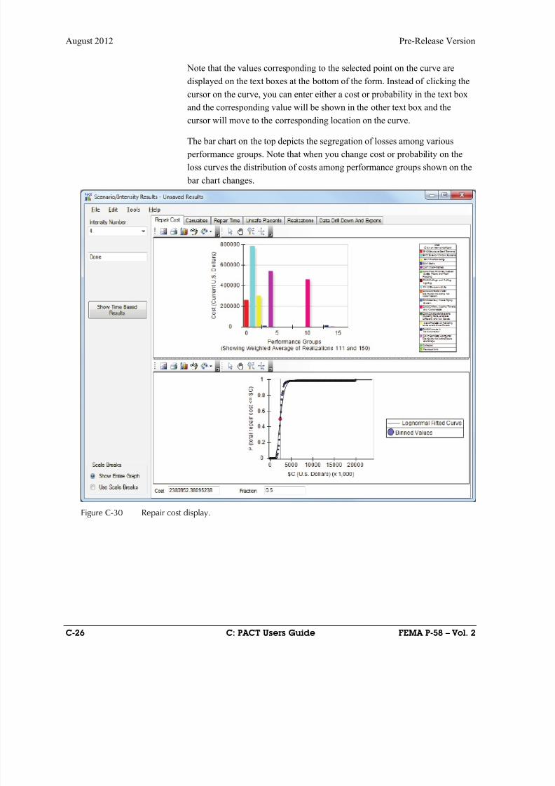
8/12/2019 Seismic Performance Assessment of Buildings
http://slidepdf.com/reader/full/seismic-performance-assessment-of-buildings 312/358
August 2012 Pre-Release Version
C-26 C: PACT Users Guide FEMA P-58 – Vol. 2
Note that the values corresponding to the selected point on the curve are
displayed on the text boxes at the bottom of the form. Instead of clicking the
cursor on the curve, you can enter either a cost or probability in the text box
and the corresponding value will be shown in the other text box and the
cursor will move to the corresponding location on the curve.
The bar chart on the top depicts the segregation of losses among various
performance groups. Note that when you change cost or probability on the
loss curves the distribution of costs among performance groups shown on the
bar chart changes.
Figure C-30 Repair cost display.

8/12/2019 Seismic Performance Assessment of Buildings
http://slidepdf.com/reader/full/seismic-performance-assessment-of-buildings 313/358
Pre-Release Version August 2012
FEMA P-58 – Vol. 2 C: PACT Users Guide C-27
C.5.4.1.2 Casualties Tab
Two sets of graphs are shown on this form. One set for fatalities (of the left)
and the other set for injuries. You can point your cursor at the lines
separating the graphs, hold the mouse key down and drag a line to resize the
graphs. You select the desired Scenario/Intensity number using the drop
down list at the top left of the form.
The graphs at the bottom of the form depict casualty probabilities associated
with the selected Scenario/Intensity. As before, by default the cursor on the
graphs is placed at the median value. However, you can click anywhere on a
curve to examine probabilities associated with various casualties.
Note that the values corresponding to the selected point on the curve are
displayed on the text boxes at the bottom of the form. Instead of clicking the
cursor on the curve, you can enter either a cost or probability in the text boxand the corresponding value will be shown in the other text box and the
cursor will move to the corresponding location on the curve.
The bar chart on the top depicts the segregation of casualties caused by
various performance groups and collapse (if occurring). Note that when you
change the curser position on the bottom curves the distribution of casualties
per performance groups shown on the corresponding bar chart changes.
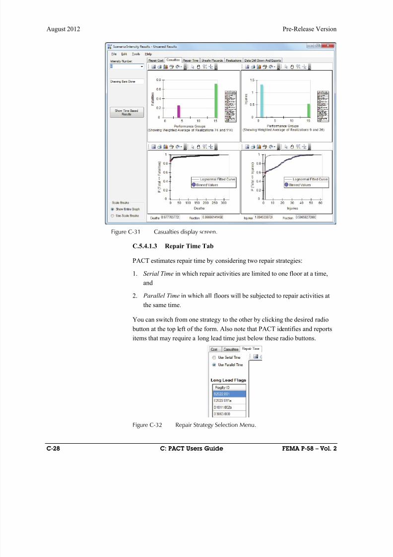
8/12/2019 Seismic Performance Assessment of Buildings
http://slidepdf.com/reader/full/seismic-performance-assessment-of-buildings 314/358
August 2012 Pre-Release Version
C-28 C: PACT Users Guide FEMA P-58 – Vol. 2
Figure C-31 Casualties display screen.
C.5.4.1.3 Repair Time Tab
PACT estimates repair time by considering two repair strategies:
1. Serial Time in which repair activities are limited to one floor at a time,and
2. Parallel Time in which all floors will be subjected to repair activities at
the same time.
You can switch from one strategy to the other by clicking the desired radio
button at the top left of the form. Also note that PACT identifies and reports
items that may require a long lead time just below these radio buttons.
Figure C-32 Repair Strategy Selection Menu.
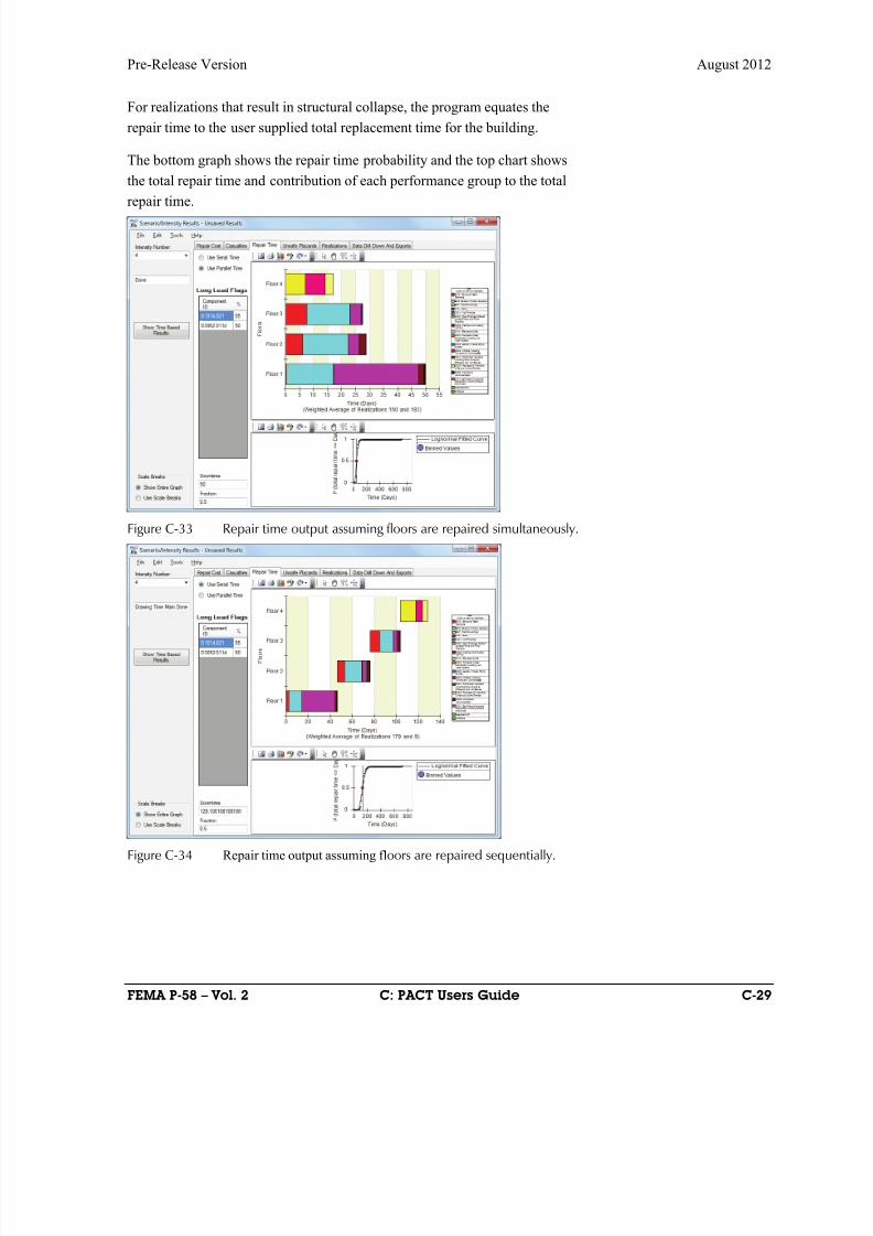
8/12/2019 Seismic Performance Assessment of Buildings
http://slidepdf.com/reader/full/seismic-performance-assessment-of-buildings 315/358
Pre-Release Version August 2012
FEMA P-58 – Vol. 2 C: PACT Users Guide C-29
For realizations that result in structural collapse, the program equates the
repair time to the user supplied total replacement time for the building.
The bottom graph shows the repair time probability and the top chart shows
the total repair time and contribution of each performance group to the total
repair time.
Figure C-33 Repair time output assuming floors are repaired simultaneously.
Figure C-34 Repair time output assuming floors are repaired sequentially.
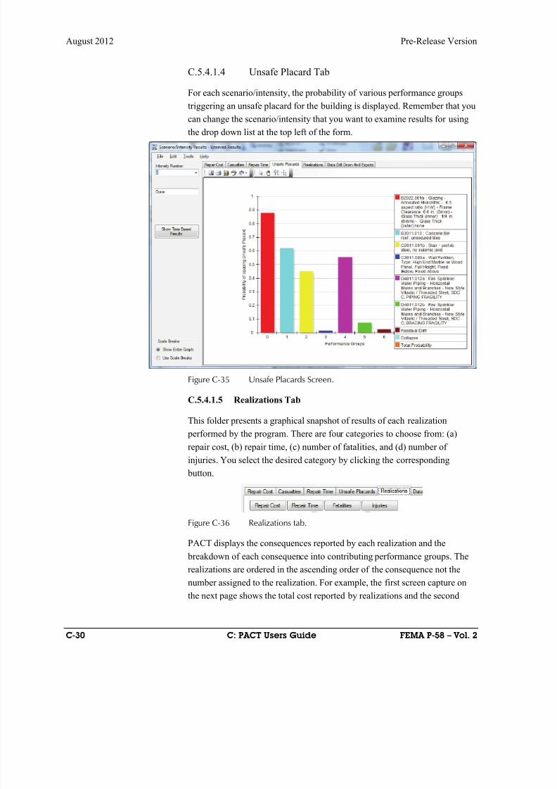
8/12/2019 Seismic Performance Assessment of Buildings
http://slidepdf.com/reader/full/seismic-performance-assessment-of-buildings 316/358
August 2012 Pre-Release Version
C-30 C: PACT Users Guide FEMA P-58 – Vol. 2
C.5.4.1.4 Unsafe Placard Tab
For each scenario/intensity, the probability of various performance groups
triggering an unsafe placard for the building is displayed. Remember that you
can change the scenario/intensity that you want to examine results for using
the drop down list at the top left of the form.
Figure C-35 Unsafe Placards Screen.
C.5.4.1.5 Realizations Tab
This folder presents a graphical snapshot of results of each realization
performed by the program. There are four categories to choose from: (a)
repair cost, (b) repair time, (c) number of fatalities, and (d) number of
injuries. You select the desired category by clicking the corresponding
button.
Figure C-36 Realizations tab.
PACT displays the consequences reported by each realization and the
breakdown of each consequence into contributing performance groups. The
realizations are ordered in the ascending order of the consequence not the
number assigned to the realization. For example, the first screen capture on
the next page shows the total cost reported by realizations and the second
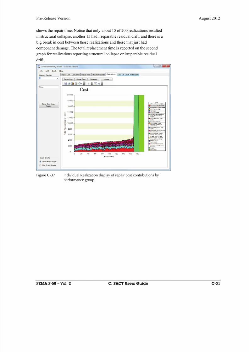
8/12/2019 Seismic Performance Assessment of Buildings
http://slidepdf.com/reader/full/seismic-performance-assessment-of-buildings 317/358
Pre-Release Version August 2012
FEMA P-58 – Vol. 2 C: PACT Users Guide C-31
shows the repair time. Notice that only about 15 of 200 realizations resulted
in structural collapse, another 15 had irreparable residual drift, and there is a
big break in cost between those realizations and those that just had
component damage. The total replacement time is reported on the second
graph for realizations reporting structural collapse or irreparable residual
drift.
Figure C-37 Individual Realization display of repair cost contributions byperformance group.
Cost
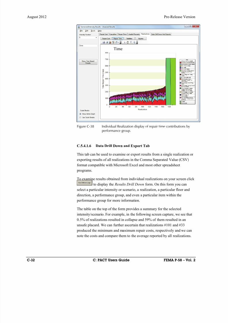
8/12/2019 Seismic Performance Assessment of Buildings
http://slidepdf.com/reader/full/seismic-performance-assessment-of-buildings 318/358
August 2012 Pre-Release Version
C-32 C: PACT Users Guide FEMA P-58 – Vol. 2
Figure C-38 Individual Realization display of repair time contributions byperformance group.
C.5.4.1.6 Data Drill Down and Export Tab
This tab can be used to examine or export results from a single realization or
exporting results of all realizations in the Comma Separated Value (CSV)
format compatible with Microsoft Excel and most other spreadsheet
programs.
To examine results obtained from individual realizations on your screen click
to display the Results Drill Down form. On this form you can
select a particular intensity or scenario, a realization, a particular floor and
direction, a performance group, and even a particular item within the
performance group for more information.
The table on the top of the form provides a summary for the selected
intensity/scenario. For example, in the following screen capture, we see that
0.5% of realizations resulted in collapse and 59% of them resulted in an
unsafe placard. We can further ascertain that realizations #101 and #33
produced the minimum and maximum repair costs, respectively and we can
note the costs and compare them to the average reported by all realizations.
Time
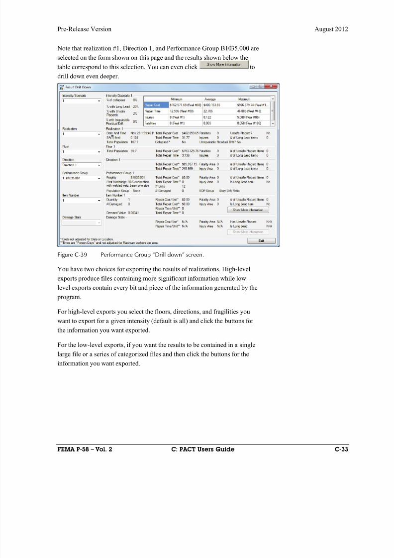
8/12/2019 Seismic Performance Assessment of Buildings
http://slidepdf.com/reader/full/seismic-performance-assessment-of-buildings 319/358
Pre-Release Version August 2012
FEMA P-58 – Vol. 2 C: PACT Users Guide C-33
Note that realization #1, Direction 1, and Performance Group B1035.000 are
selected on the form shown on this page and the results shown below the
table correspond to this selection. You can even click to
drill down even deeper.
Figure C-39 Performance Group “Drill down” screen.
You have two choices for exporting the results of realizations. High-level
exports produce files containing more significant information while low-
level exports contain every bit and piece of the information generated by the
program.
For high-level exports you select the floors, directions, and fragilities you
want to export for a given intensity (default is all) and click the buttons for
the information you want exported.
For the low-level exports, if you want the results to be contained in a single
large file or a series of categorized files and then click the buttons for the
information you want exported.
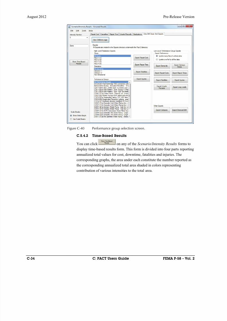
8/12/2019 Seismic Performance Assessment of Buildings
http://slidepdf.com/reader/full/seismic-performance-assessment-of-buildings 320/358
August 2012 Pre-Release Version
C-34 C: PACT Users Guide FEMA P-58 – Vol. 2
Figure C-40 Performance group selection screen.
C.5.4.2 Time-Based Results
You can click on any of the Scenario/Intensity Results forms to
display time-based results form. This form is divided into four parts reporting
annualized total values for cost, downtime, fatalities and injuries. The
corresponding graphs, the area under each constitute the number reported as
the corresponding annualized total area shaded in colors representing
contribution of various intensities to the total area.
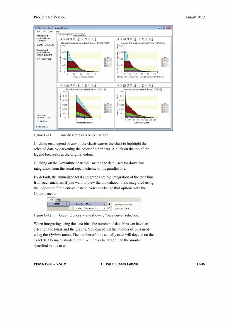
8/12/2019 Seismic Performance Assessment of Buildings
http://slidepdf.com/reader/full/seismic-performance-assessment-of-buildings 321/358
Pre-Release Version August 2012
FEMA P-58 – Vol. 2 C: PACT Users Guide C-35
Figure C-41 Time-based results output screen.
Clicking on a legend of any of the charts causes the chart to highlight the
selected data by darkening the color of other data. A click on the top of the
legend box restores the original colors.
Clicking on the Downtime chart will switch the data used for downtime
integration from the serial repair scheme to the parallel one.
By default, the annualized total and graphs are the integration of the data bins
from each analysis. If you want to view the annualized totals integrated using
the lognormal fitted curves instead, you can change that options with the
Options menu.
Figure C-42 Graph Options Menu showing “base curve” selection.
When integrating using the data bins, the number of data bins can have an
effect on the totals and the graphs. You can adjust the number of bins used
using the Options menu. The number of bins actually used will depend on the
exact data being evaluated, but it will never be larger than the number
specified by the user.
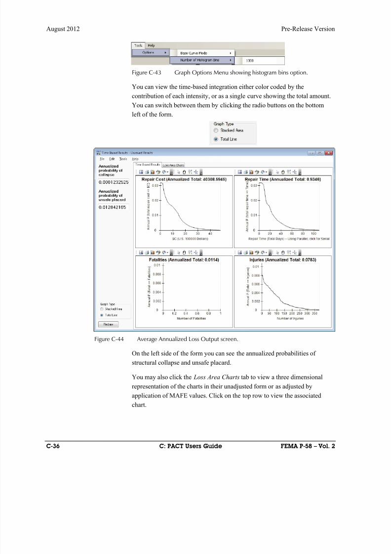
8/12/2019 Seismic Performance Assessment of Buildings
http://slidepdf.com/reader/full/seismic-performance-assessment-of-buildings 322/358
August 2012 Pre-Release Version
C-36 C: PACT Users Guide FEMA P-58 – Vol. 2
Figure C-43 Graph Options Menu showing histogram bins option.
You can view the time-based integration either color coded by the
contribution of each intensity, or as a single curve showing the total amount.
You can switch between them by clicking the radio buttons on the bottom
left of the form.
Figure C-44 Average Annualized Loss Output screen.
On the left side of the form you can see the annualized probabilities of
structural collapse and unsafe placard.
You may also click the Loss Area Charts tab to view a three dimensional
representation of the charts in their unadjusted form or as adjusted by
application of MAFE values. Click on the top row to view the associated
chart.
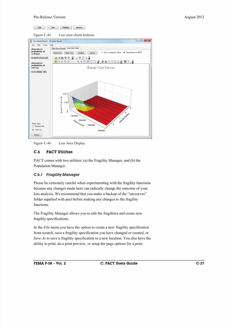
8/12/2019 Seismic Performance Assessment of Buildings
http://slidepdf.com/reader/full/seismic-performance-assessment-of-buildings 323/358
Pre-Release Version August 2012
FEMA P-58 – Vol. 2 C: PACT Users Guide C-37
Figure C-45 Loss area charts buttons.
Figure C-46 Loss Area Display.
C.6 PACT Utilities
PACT comes with two utilities: (a) the Fragility Manager, and (b) thePopulation Manager.
C.6.1 Fragility Manager
Please be extremely careful when experimenting with the fragility functions
because any changes made here can radically change the outcome of your
loss analysis. We recommend that you make a backup of the “\atccurves”
folder supplied with pact before making any changes to the fragility
functions.
The Fragility Manager allows you to edit the fragilities and create newfragility specifications.
In the File menu you have the option to create a new fragility specification
from scratch, save a fragility specification you have changed or created, or
Save As to save a fragility specification to a new location. You also have the
ability to print, do a print preview, or setup the page options for a print.
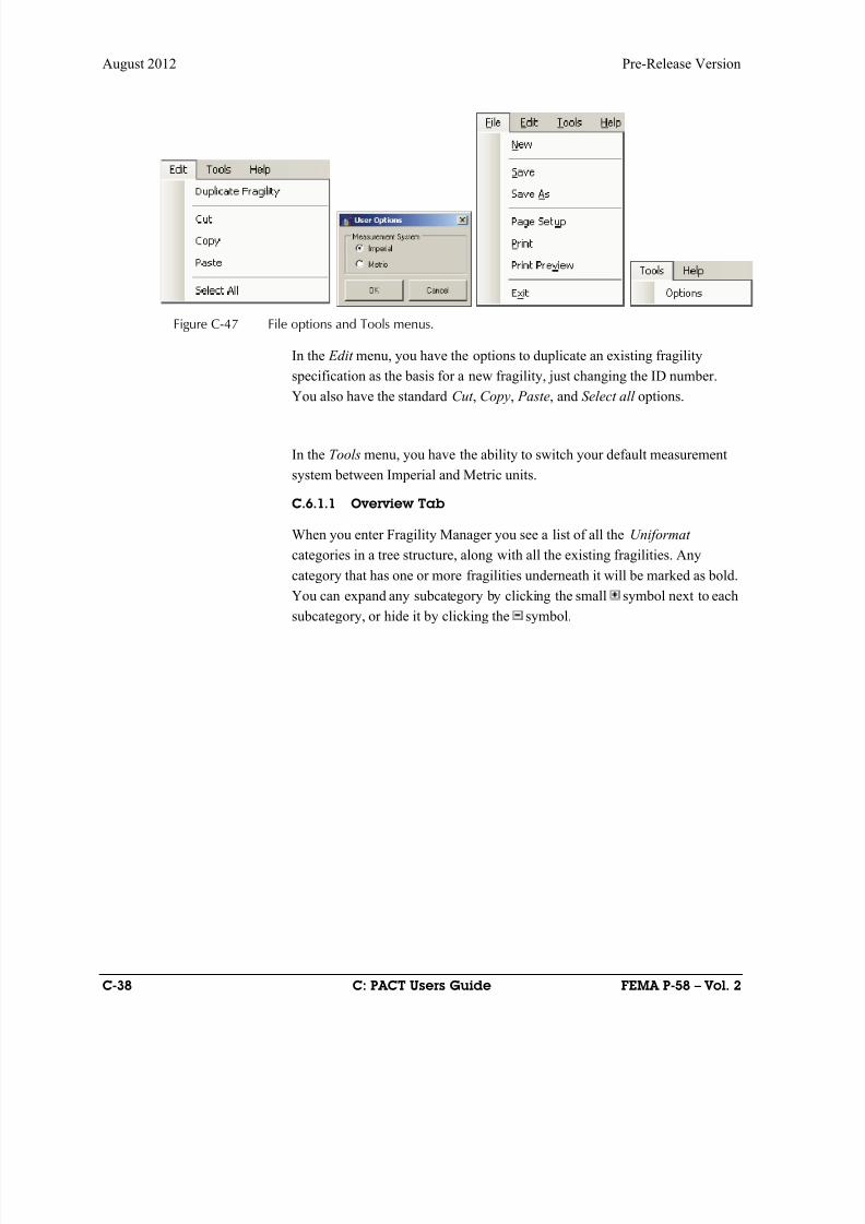
8/12/2019 Seismic Performance Assessment of Buildings
http://slidepdf.com/reader/full/seismic-performance-assessment-of-buildings 324/358
August 2012 Pre-Release Version
C-38 C: PACT Users Guide FEMA P-58 – Vol. 2
Figure C-47 File options and Tools menus.
In the Edit menu, you have the options to duplicate an existing fragility
specification as the basis for a new fragility, just changing the ID number.
You also have the standard Cut , Copy, Paste, and Select all options.
In the Tools menu, you have the ability to switch your default measurement
system between Imperial and Metric units.
C.6.1.1 Overview Tab
When you enter Fragility Manager you see a list of all the Uniformat
categories in a tree structure, along with all the existing fragilities. Any
category that has one or more fragilities underneath it will be marked as bold.
You can expand any subcategory by clicking the small symbol next to eachsubcategory, or hide it by clicking the symbol.
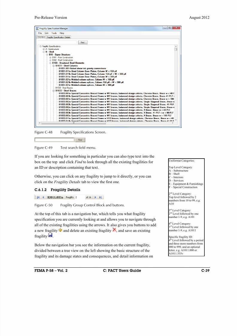
8/12/2019 Seismic Performance Assessment of Buildings
http://slidepdf.com/reader/full/seismic-performance-assessment-of-buildings 325/358
Pre-Release Version August 2012
FEMA P-58 – Vol. 2 C: PACT Users Guide C-39
Uniformat Categories:
Top Level Category:
A – SubstructureB – Shell
C – Interiors
D – Services
E – Equipment & FurnishingsF – Special Construction
2nd Level Category:
Top level followed by 2
numbers from 10 to 99, e.g.A10
3rd Level Category:
2nd Level followed by onenumber 1-9, e.g. A101
4th Level Category:
3rd Level followed by one
number 1-9, e.g. A1011
Specific fragility ID:
4th Level followed by a period
and three more numbers from
000 to 999, and an optionalletter, e.g. A1011.000 or
A1011.555v
Figure C-48 Fragility Specifications Screen.
Figure C-49 Text search field menu.
If you are looking for something in particular you can also type text into the
box on the top and click Find to look through all the existing fragilities for
an ID or description containing that text.
Otherwise, you can click on any fragility to jump to it directly, or you can
click on the Fragility Details tab to view the first one.
C.6.1.2 Fragility Details
Figure C-50 Fragility Group Control Block and buttons.
At the top of this tab is a navigation bar, which tells you what fragility
specification you are currently looking at and allows you to navigate throughall of the existing fragilities using the arrows. It also gives you buttons to add
a new fragility and delete an existing fragility , and save an existing
fragility .
Below the navigation bar you see the information on the current fragility,
divided between a tree view on the left showing the basic structure of the
fragility and its damage states and consequences, and detail information on

8/12/2019 Seismic Performance Assessment of Buildings
http://slidepdf.com/reader/full/seismic-performance-assessment-of-buildings 326/358
August 2012 Pre-Release Version
C-40 C: PACT Users Guide FEMA P-58 – Vol. 2
the right. You can shift the border between the tree view and the detail
information left or right by clicking and dragging on the border between
them.
Figure C-51 Fragility Manager Data Screen.
When you add a new fragility, or duplicate an existing one, the first thing the
Fragility Manager will ask you is for the Uniformat ID number that you
would like to use. It is recommended that you study the Uniformat categories
that are shown on the overview tab to try and find a category that fits the
item you are creating a fragility for. The format of the ID field that the
fragility manager expects is a single upper case letter between A-F followed
by two digits from 10 to 99, two more digits from 11 to 99, followed by a
period, then 3 more digits from 000 to 999, followed by an optional lower
case letter from a to z.
C.6.1.3 Fragility Structure Tree View
The fragility structure consists of general information for the fragility and
various damage state groups and sub-damage state groups, individual
damage states, and consequences.
The easiest structure is that of a sequential fragility. It consists of general
information, a single damage state group (designated with the title of
“damage State Type”), one or more individual damage states, and
consequences for each of those damage states.

8/12/2019 Seismic Performance Assessment of Buildings
http://slidepdf.com/reader/full/seismic-performance-assessment-of-buildings 327/358
Pre-Release Version August 2012
FEMA P-58 – Vol. 2 C: PACT Users Guide C-41
Here is an example of a simple sequentialragility with 3 damage states.
Here is an example of a simultaneousragility with general info, a single “master”
damage state group with a single damage state, and a simultaneous sub-damage state group under that with four damage states,each with its own consequence.
Some very complicated fragility structures consisting of multiple sub-damage state groups and sub-sub-damage state groupsof several different types.
Figure C-52 Fragility Manager Data Screen.
The structure of a mutually exclusive or simultaneous fragility is more
complicated. In either case, you have a “master” sequential damage state
group (designated with the title of “Damage State Type”) with only a single
damage state. This damage state is used to determine if the item in question
is damaged at all based on the EDP value of a particular realization. If it is
determined that there is some damage, you have a sub-damage state group,
marked as either simultaneous or mutually exclusive, with two or more
damage states to determine the exact kind of damage, with consequence
functions for each damage state.
PACT does not limit you to these options. You could have multiple
damage state groups of all different types nested underneath each
other, but the utility of these options is probably limited.
Figure C-53 Complex damage state logic tree.
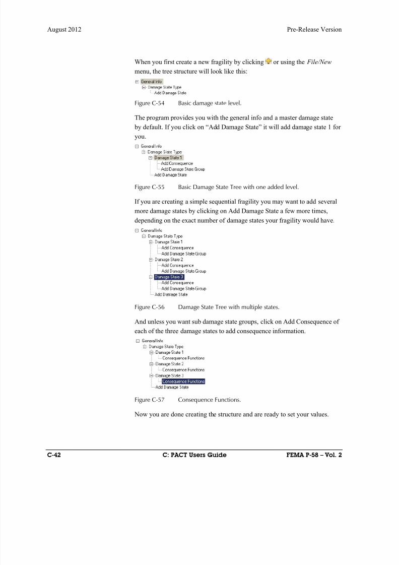
8/12/2019 Seismic Performance Assessment of Buildings
http://slidepdf.com/reader/full/seismic-performance-assessment-of-buildings 328/358
August 2012 Pre-Release Version
C-42 C: PACT Users Guide FEMA P-58 – Vol. 2
When you first create a new fragility by clicking or using the File/New
menu, the tree structure will look like this:
Figure C-54 Basic damage state level.
The program provides you with the general info and a master damage state
by default. If you click on “Add Damage State” it will add damage state 1 for
you.
Figure C-55 Basic Damage State Tree with one added level.
If you are creating a simple sequential fragility you may want to add several
more damage states by clicking on Add Damage State a few more times,
depending on the exact number of damage states your fragility would have.
Figure C-56 Damage State Tree with multiple states.
And unless you want sub damage state groups, click on Add Consequence of
each of the three damage states to add consequence information.
Figure C-57 Consequence Functions.
Now you are done creating the structure and are ready to set your values.
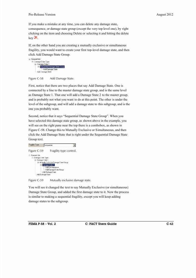
8/12/2019 Seismic Performance Assessment of Buildings
http://slidepdf.com/reader/full/seismic-performance-assessment-of-buildings 329/358
Pre-Release Version August 2012
FEMA P-58 – Vol. 2 C: PACT Users Guide C-43
If you make a mistake at any time, you can delete any damage state,
consequence, or damage state group (except the very top level one), by right
clicking on the item and choosing Delete or selecting it and hitting the delete
key .
If, on the other hand you are creating a mutually exclusive or simultaneousfragility, you would want to create your first top-level damage state, and then
click Add Damage State Group.
Figure C-58 Add Damage State.
First, notice that there are two places that say Add Damage State. One is
connected by a line to the master damage state group, and is the same levelas Damage State 1. That one will add a Damage State 2 to the master group,
and is probably not what you want to do at this point. The other is under the
level of the subgroup, and will add a damage state to this subgroup, and is the
one you probably want.
Second, notice that it says “Sequential Damage State Group”. When you
have selected this damage state group, as shown above in the example, you
will see on the right pane near the top there is a combobox, as shown in
Figure C-58. Change this to Mutually Exclusive or Simultaneous, and then
click the Add Damage State that is right under the Sequential Damage State
Group text.
Figure C-59 Fragility type control.
Figure C-59 Mutually exclusive damage state.
You will see it changed the text to say Mutually Exclusive (or simultaneous)
Damage State Group, and added the first damage state to it. Now the process
is similar to making a sequential fragility, except you will keep adding
damage states to the subgroup.
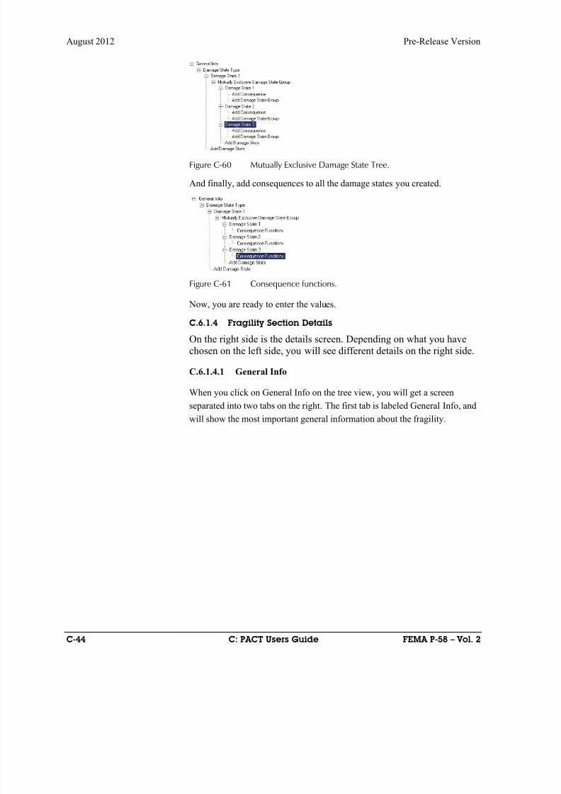
8/12/2019 Seismic Performance Assessment of Buildings
http://slidepdf.com/reader/full/seismic-performance-assessment-of-buildings 330/358
August 2012 Pre-Release Version
C-44 C: PACT Users Guide FEMA P-58 – Vol. 2
Figure C-60 Mutually Exclusive Damage State Tree.
And finally, add consequences to all the damage states you created.
Figure C-61 Consequence functions.
Now, you are ready to enter the values.
C.6.1.4 Fragility Section Details
On the right side is the details screen. Depending on what you havechosen on the left side, you will see different details on the right side.
C.6.1.4.1 General Info
When you click on General Info on the tree view, you will get a screen
separated into two tabs on the right. The first tab is labeled General Info, and
will show the most important general information about the fragility.
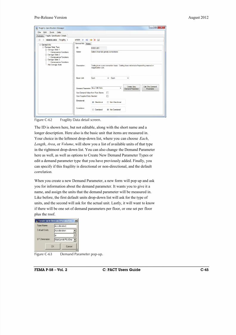
8/12/2019 Seismic Performance Assessment of Buildings
http://slidepdf.com/reader/full/seismic-performance-assessment-of-buildings 331/358
Pre-Release Version August 2012
FEMA P-58 – Vol. 2 C: PACT Users Guide C-45
Figure C-62 Fragility Data detail screen.
The ID is shown here, but not editable, along with the short name and a
longer description. Here also is the basic unit that items are measured in.
Your choice in the leftmost drop-down list, where you can choose Each,
Length, Area, or Volume, will show you a list of available units of that type
in the rightmost drop-down list. You can also change the Demand Parameter
here as well, as well as options to Create New Demand Parameter Types or
edit a demand parameter type that you have previously added. Finally, you
can specify if this fragility is directional or non-directional, and the default
correlation.
When you create a new Demand Parameter, a new form will pop up and ask
you for information about the demand parameter. It wants you to give it a
name, and assign the units that the demand parameter will be measured in.
Like before, the first default units drop-down list will ask for the type of
units, and the second will ask for the actual unit. Lastly, it will want to know
if there will be one set of demand parameters per floor, or one set per floor
plus the roof.
Figure C-63 Demand Parameter pop-up.
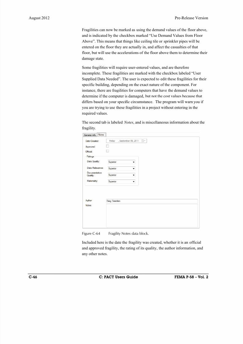
8/12/2019 Seismic Performance Assessment of Buildings
http://slidepdf.com/reader/full/seismic-performance-assessment-of-buildings 332/358
August 2012 Pre-Release Version
C-46 C: PACT Users Guide FEMA P-58 – Vol. 2
Fragilities can now be marked as using the demand values of the floor above,
and is indicated by the checkbox marked “Use Demand Values from Floor
Above”. This means that things like ceiling tile or sprinkler pipes will be
entered on the floor they are actually in, and affect the casualties of that
floor, but will use the accelerations of the floor above them to determine their
damage state.
Some fragilities will require user-entered values, and are therefore
incomplete. These fragilities are marked with the checkbox labeled “User
Supplied Data Needed”. The user is expected to edit these fragilities for their
specific building, depending on the exact nature of the component. For
instance, there are fragilities for computers that have the demand values to
determine if the computer is damaged, but not the cost values because that
differs based on your specific circumstance. The program will warn you if
you are trying to use these fragilities in a project without entering in the
required values.
The second tab is labeled Notes, and is miscellaneous information about the
fragility.
Figure C-64 Fragility Notes data block.
Included here is the date the fragility was created, whether it is an official
and approved fragility, the rating of its quality, the author information, and
any other notes.
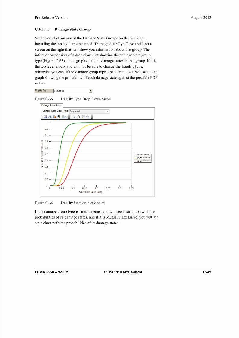
8/12/2019 Seismic Performance Assessment of Buildings
http://slidepdf.com/reader/full/seismic-performance-assessment-of-buildings 333/358
Pre-Release Version August 2012
FEMA P-58 – Vol. 2 C: PACT Users Guide C-47
C.6.1.4.2 Damage State Group
When you click on any of the Damage State Groups on the tree view,
including the top level group named “Damage State Type”, you will get a
screen on the right that will show you information about that group. The
information consists of a drop-down list showing the damage state grouptype (Figure C-65), and a graph of all the damage states in that group. If it is
the top level group, you will not be able to change the fragility type,
otherwise you can. If the damage group type is sequential, you will see a line
graph showing the probability of each damage state against the possible EDP
values.
Figure C-65 Fragility Type Drop Down Menu.
Figure C-66 Fragility function plot display.
If the damage group type is simultaneous, you will see a bar graph with the
probabilities of its damage states, and if it is Mutually Exclusive, you will see
a pie chart with the probabilities of its damage states.

8/12/2019 Seismic Performance Assessment of Buildings
http://slidepdf.com/reader/full/seismic-performance-assessment-of-buildings 334/358
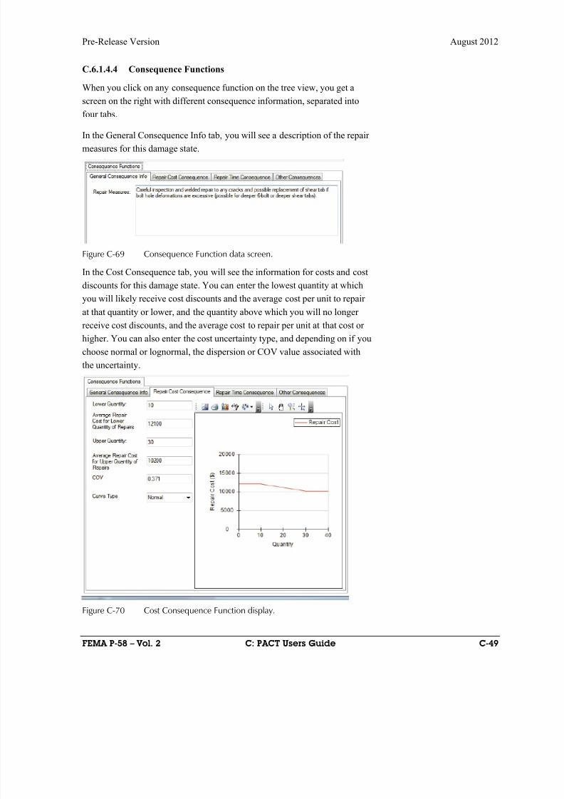
8/12/2019 Seismic Performance Assessment of Buildings
http://slidepdf.com/reader/full/seismic-performance-assessment-of-buildings 335/358
Pre-Release Version August 2012
FEMA P-58 – Vol. 2 C: PACT Users Guide C-49
C.6.1.4.4 Consequence Functions
When you click on any consequence function on the tree view, you get a
screen on the right with different consequence information, separated into
four tabs.
In the General Consequence Info tab, you will see a description of the repair
measures for this damage state.
Figure C-69 Consequence Function data screen.
In the Cost Consequence tab, you will see the information for costs and cost
discounts for this damage state. You can enter the lowest quantity at which
you will likely receive cost discounts and the average cost per unit to repair
at that quantity or lower, and the quantity above which you will no longer
receive cost discounts, and the average cost to repair per unit at that cost or
higher. You can also enter the cost uncertainty type, and depending on if you
choose normal or lognormal, the dispersion or COV value associated with
the uncertainty.
Figure C-70 Cost Consequence Function display.

8/12/2019 Seismic Performance Assessment of Buildings
http://slidepdf.com/reader/full/seismic-performance-assessment-of-buildings 336/358
August 2012 Pre-Release Version
C-50 C: PACT Users Guide FEMA P-58 – Vol. 2
In the Time Consequence tab, you will see the information for time and time
discounts for this damage state. The information is identical to that of the
Cost Consequence tab.
Figure C-71 Repair Time Consequence Function display.
Finally, in the Other Consequences tab, we have information on the Red Flag
consequences, Non-Collapse Casualty consequences, and Long Lead
consequences.
Figure C-72 Other Consequence data entry screen.

8/12/2019 Seismic Performance Assessment of Buildings
http://slidepdf.com/reader/full/seismic-performance-assessment-of-buildings 337/358
Pre-Release Version August 2012
FEMA P-58 – Vol. 2 C: PACT Users Guide C-51
Here you can specify if you would like to use Unsafe Placard consequences
or not, and if so, what is the fraction of the total quantities required to trigger
a red flag. The program will count all the items of this type in the building,
and count how many of those items are in this damage state. If the ratio is
higher than the median value here (adjusted by the dispersion) for a
particular realization, it will be marked as getting a red flag. It will not add
different damage states together, even different damage states for the same
fragility.
You can also specify Non-Collapse Casualties here. You first give the
information of how much floor is affected by an item in this damage state,
then what the death rate and serious injury rate is for anyone in that affected
area.
Finally, you can specify if an item in this damage state is considered a long
lead item.
C.6.2 Population Manager
Please be extremely careful when experimenting with the population
library because any changes made here can radically change the
outcome of your casulaty loss analysis. We recommend that you make
a backup of the population library supplied with pact before makingany changes to this library.
Figure C-73 Population Model entry.
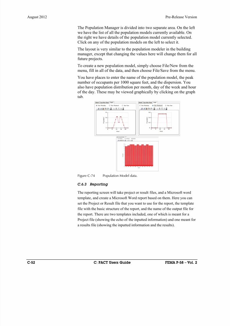
8/12/2019 Seismic Performance Assessment of Buildings
http://slidepdf.com/reader/full/seismic-performance-assessment-of-buildings 338/358
August 2012 Pre-Release Version
C-52 C: PACT Users Guide FEMA P-58 – Vol. 2
The Population Manager is divided into two separate area. On the left
we have the list of all the population models currently available. Onthe right we have details of the population model currently selected.
Click on any of the population models on the left to select it.
The layout is very similar to the population modeler in the building
manager, except that changing the values here will change them for allfuture projects.
To create a new population model, simply choose File/New from the
menu, fill in all of the data, and then choose File/Save from the menu.
You have places to enter the name of the population model, the peak
number of occupants per 1000 square feet, and the dispersion. Youalso have population distribution per month, day of the week and hour
of the day. These may be viewed graphically by clicking on the graph
tab.
Figure C-74 Population Model data. C.6.3 Reporting
The reporting screen will take project or result files, and a Microsoft word
template, and create a Microsoft Word report based on them. Here you can
set the Project or Result file that you want to use for the report, the template
file with the basic structure of the report, and the name of the output file for
the report. There are two templates included, one of which is meant for aProject file (showing the echo of the inputted information) and one meant for
a results file (showing the inputted information and the results).
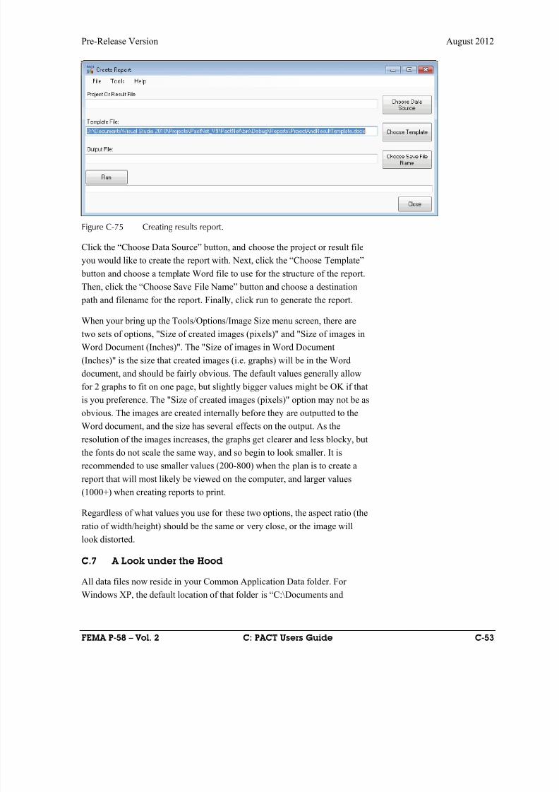
8/12/2019 Seismic Performance Assessment of Buildings
http://slidepdf.com/reader/full/seismic-performance-assessment-of-buildings 339/358
Pre-Release Version August 2012
FEMA P-58 – Vol. 2 C: PACT Users Guide C-53
Figure C-75 Creating results report.
Click the “Choose Data Source” button, and choose the project or result file
you would like to create the report with. Next, click the “Choose Template” button and choose a template Word file to use for the structure of the report.
Then, click the “Choose Save File Name” button and choose a destination
path and filename for the report. Finally, click run to generate the report.
When your bring up the Tools/Options/Image Size menu screen, there are
two sets of options, "Size of created images (pixels)" and "Size of images in
Word Document (Inches)". The "Size of images in Word Document
(Inches)" is the size that created images (i.e. graphs) will be in the Word
document, and should be fairly obvious. The default values generally allow
for 2 graphs to fit on one page, but slightly bigger values might be OK if thatis you preference. The "Size of created images (pixels)" option may not be as
obvious. The images are created internally before they are outputted to the
Word document, and the size has several effects on the output. As the
resolution of the images increases, the graphs get clearer and less blocky, but
the fonts do not scale the same way, and so begin to look smaller. It is
recommended to use smaller values (200-800) when the plan is to create a
report that will most likely be viewed on the computer, and larger values
(1000+) when creating reports to print.
Regardless of what values you use for these two options, the aspect ratio (the
ratio of width/height) should be the same or very close, or the image will
look distorted.
C.7 A Look under the Hood
All data files now reside in your Common Application Data folder. For
Windows XP, the default location of that folder is “C:\Documents and

8/12/2019 Seismic Performance Assessment of Buildings
http://slidepdf.com/reader/full/seismic-performance-assessment-of-buildings 340/358
August 2012 Pre-Release Version
C-54 C: PACT Users Guide FEMA P-58 – Vol. 2
Settings\All Users\Application Data\Pact”, and for Windows 7 it is
“C:\ProgramData\Pact”.
C.7.1 Project Files
All building and project information inputted for a particular project are
saved in a single XML file with the project name in the Projects sub-folder
under the folder that you installed PACT at. If you used the default path for
installing PACT, the project files may be found under your data folder in
“\PACT\Projects”. Although XML files are text files that can be viewed and
changed using any text or word processor you should be extremely careful if
you want to manipulate these files as even minor manual changes may render
a project file unusable. You can of course copy a project file for
transportation to another computer or for archival purposes with no adverse
effects.
C.7.2 Results Files
All result information if saved, is saved in a single file with the result name
in the Projects sub-folder under the folder that you installed PACT at. If you
used the default path for installing PACT, the project files may be found in
your data folder at “\PACT\Projects”. You can choose to save results files as
binary files, with the file extension .bin, or you can save them as XML files,
with the file extension XML. Binary files will be smaller, typically half the
size of XML files, and be much faster to load and save. Results files can be
quite large, so this is not a trivial concern. Binary files can only be read by
the PACT Result Viewer. Binary files have been reported to cause out ofmemory errors when being saved or loaded, so if you have issues using them,
try the XML files. XML files, while much larger, can be read by any text
editor, and can easily be parsed and manipulated by other programs. Either
file format contains the original project file, all the fragilities used by that
project, and all the result information, including every single analysis,
realization, performance group, damage state, and even every random
number used in any calculation.
C.7.3 Fragility Specification Files
Fragility specifications are directories and XML files that bear the same
identifier as the fragility specification they represent. For each fragility
specification, there is a folder with the same name as the fragility ID,
containing an XML file and any representative photos of the damage states
associated with the fragility function. These folders are stored in a subfolder
under the folder that you installed PACT at. If you used the default path for
installing PACT, these files may be found under the data directory in
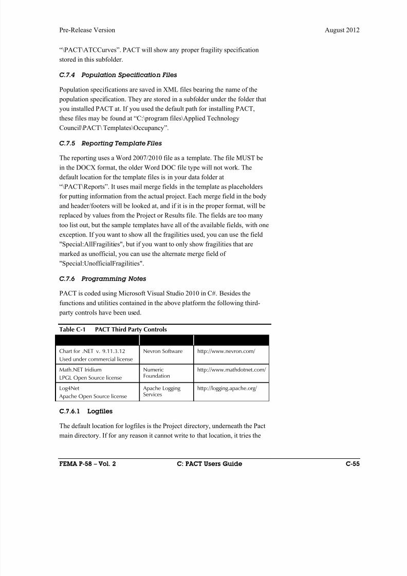
8/12/2019 Seismic Performance Assessment of Buildings
http://slidepdf.com/reader/full/seismic-performance-assessment-of-buildings 341/358
Pre-Release Version August 2012
FEMA P-58 – Vol. 2 C: PACT Users Guide C-55
“\PACT\ATCCurves”. PACT will show any proper fragility specification
stored in this subfolder.
C.7.4 Population Specification Files
Population specifications are saved in XML files bearing the name of the
population specification. They are stored in a subfolder under the folder that
you installed PACT at. If you used the default path for installing PACT,
these files may be found at “C:\program files\Applied Technology
Council\PACT\ Templates\Occupancy”.
C.7.5 Reporting Template Files
The reporting uses a Word 2007/2010 file as a template. The file MUST be
in the DOCX format, the older Word DOC file type will not work. The
default location for the template files is in your data folder at
“\PACT\Reports”. It uses mail merge fields in the template as placeholdersfor putting information from the actual project. Each merge field in the body
and header/footers will be looked at, and if it is in the proper format, will be
replaced by values from the Project or Results file. The fields are too many
too list out, but the sample templates have all of the available fields, with one
exception. If you want to show all the fragilities used, you can use the field
"Special:AllFragilities", but if you want to only show fragilities that are
marked as unofficial, you can use the alternate merge field of
"Special:UnofficialFragilities".
C.7.6 Programming Notes
PACT is coded using Microsoft Visual Studio 2010 in C#. Besides the
functions and utilities contained in the above platform the following third-
party controls have been used.
Table C-1 PACT Third Party Controls
Control Name Vendor Link
Chart for .NET v. 9.11.3.12
Used under commercial license
Nevron Software http://www.nevron.com/
Math.NET Iridium
LPGL Open Source license
Numeric
Foundation
http://www.mathdotnet.com/
Log4Net
Apache Open Source license
Apache LoggingServices
http://logging.apache.org/
C.7.6.1 Logfiles
The default location for logfiles is the Project directory, underneath the Pact
main directory. If for any reason it cannot write to that location, it tries the
8/12/2019 Seismic Performance Assessment of Buildings
http://slidepdf.com/reader/full/seismic-performance-assessment-of-buildings 342/358
August 2012 Pre-Release Version
C-56 C: PACT Users Guide FEMA P-58 – Vol. 2
Local Application Data path, which defaults to C:\Documents and
Settings\%username%\Local Settings\Application Data in Windows XP, or
C:\Users\%username%\AppData\Local in Windows 7, where %username%
is the your current username.
Please send the logfile when reporting bugs, it makes tracking down bugs alot easier.
8/12/2019 Seismic Performance Assessment of Buildings
http://slidepdf.com/reader/full/seismic-performance-assessment-of-buildings 343/358
Pre-Release Version August 2012
ATC-58-1 – Vol. 2 D: Normative Quantity Estimation Tool D-1
Appendix D
Normative Quantity EstimationTool
D.1 Introduction
The purpose of the Normative Quantity Estimation tool provided in
Volume 3 is to assist the user when establishing the quantities of various
building components for entry into the building performance model.
The tool assumes that the quantity of all building components can be
expressed as a ratio of the number of instances of that component typedivided into the floor gross area. The tool requires as input a listing of the
floors of the building and the gross area per floor. The tool produces a floor-
by-floor list of the component types and the quantities of those components
for input into PACT. To facilitate the building definition, the tool includes
predefined occupancy types which package quantity data for the components
commonly appearing in that occupancy. Eight predefined occupancies are
included with options to add additional occupancies. Up to three
occupancies may be assigned to a single floor.
D.2 Usage Notes Cells with color shading may be changed by the user. Cells with white
background are calculated or created as the tool executes. White background
cells should not be changed or moved. Columns or rows of data should not
be added or deleted except where specifically noted.
Pop up notes have been included to further explain options within the
spreadsheet. A red triangle at the upper right of a cell indicates a pop up
note. Hovering over the cell will display the note.
The tool uses Excel macros. The macros must be enabled in order for the
tool to run. The spreadsheet was created in Excel Office 2010 version
14.0.6106.5005 as a macro enabled Excel file (.xlsm).
D.3 Suggested Steps to Enter and Summarize a Building
The following provides the suggested steps to operate this tool.
8/12/2019 Seismic Performance Assessment of Buildings
http://slidepdf.com/reader/full/seismic-performance-assessment-of-buildings 344/358
August 2012 Pre-Release Version
D-2 D: Normative Quantity Estimation Tool ATC-58-1 – Vol. 2
Step 1. Enter the Building Floors and Occupancies to the Building Summary
Tab, Building Definition Table. Enter the uppermost floor first, working
down the building.
Step 2. If desired, edit the component quantity values on the Normative
Worksheet Tab, Building Occupancy Component Matrix. (This is notnecessary if the user wishes to use the assumed 50th percentile quantity
values provided with the tool.)
Step 3. On the Building Summary Tab, select the filtering and or summation
settings. These settings will eliminate incomplete or zero quantity
components, round discreet quantity components to the next larger integer
quantity, and provide summed quantity values for certain components.
Step 4. Confirm the component types selected on the Normative Worksheet
Tab are appropriate given the building size and seismic demands. More
specifically, component fragility files listed in the PACT Database are
seismic demand dependent and size dependent. The user should at very least
confirm the following:
That the components selected are appropriate for the seismic demand of
the building. (The component name provides the assumed seismic
demand.)
That an appropriate selection has been made for those components with
variable unit quantity when discreet quantity output will be provided.
For example, the PACT Database has three chillers defined that provide
between 350 and 1000 Tons of cooling. It would be a poor choice to
select the 1000 Ton chiller in a building that requires 350 Tons cooling
as this would result in an overestimation of consequence should PACT
predict damage to the chiller.
Step 5. Press the “Compile” button on the Building Summary tab. This will
execute the program and fill in the “Component Summary Matrix” output on
the Building Summary Tab.
Step 6. The Component Summary Matrix on the Building Summary tab lists
each components on each floor by occupancy for input to PACT. The
quantity of each component is determined from the occupancy component
unit quantity adjusted to reflect the floor areas assigned in STEP 1.
Step 7. Review the actual quantity data provided in the Component
Summary Matrix output to confirm the components selected are appropriate
given the building size and quantity of discreet units required. (The

8/12/2019 Seismic Performance Assessment of Buildings
http://slidepdf.com/reader/full/seismic-performance-assessment-of-buildings 345/358
Pre-Release Version August 2012
ATC-58-1 – Vol. 2 D: Normative Quantity Estimation Tool D-3
Component Summary Matrix contains a listing of the actual component
quantity as well as the assumed PACT Database unit quantity.)
D.4 Building Summary Tab – Building Definition Table
The Building Summary tab contains a Building Definition Table to be input
by the user. Within this table each floor is defined by its total floor area and
up to three occupancies. To define a building, the user first inputs the name
of each floor (starting at the roof) as well as the total floor area on each floor.
The user then selects the occupancy types present on each floor and assigns a
percentage of the total floor area to each occupancy. The user must also
provide a floor number for later reference in the output summary. The floor
name can be any alphanumeric entry; the floor number must be an integer
value starting at 1 at the first floor.
D.5 Building Summary Tab – Component Summary
Matrix
The Building Summary Tab also contains the program output: a floor-by-
floor list of component types for input into PACT referred to as the
Component Summary Matrix. This matrix is created by pressing the
“Compile” button on the Building Summary Tab. The matrix is ordered by
floor, then occupancy type.
For reference, the Component Summary Matrix also reports the actual
quantity of each component on a line by line basis. During the development
of the PACT fragility files, each component was assumed to have a certain
quantity when defining the cost and other consequences. The “Actual
Quantity” value reported recognizes this assumed PACT component quantity
and multiplies it by the user input building occupancy area and per
occupancy unit quantity defined in the Building Occupancy Component
Matrix. The “Actual Quantity” value can be used to identify erroneous or
inappropriate quantity data and or assumptions.
Several options are provided for filtering and summarizing the component
quantity data, the following section provides further discussion of these
additional features.
D.6 Building Summary Tab – Additional Features
The Building Summary tab contains four additional data processing features.
These features may be enabled using the ratio buttons next to the “Compile”
button. Each feature is described below.

8/12/2019 Seismic Performance Assessment of Buildings
http://slidepdf.com/reader/full/seismic-performance-assessment-of-buildings 346/358
August 2012 Pre-Release Version
D-4 D: Normative Quantity Estimation Tool ATC-58-1 – Vol. 2
D.6.1 Filtering of Incomplete Data
The tool allows incomplete data to be eliminated from the Component
Summary Matrix. This option may be selected using the buttons next to the
Compile button on the Building Summary tab. If the user has chosen to
“ignore incomplete data,” any component types with a unit mismatch will beconsidered incomplete and will not be listed when the tool is run.
D.6.2 Filtering of Zero Quantity Data
The tool can be set to check if the occupancy category produces a component
with zero quantity. If the user has chosen to “ignore zero data,” any
component types producing zero quantity will not be listed in the Component
Summary Matrix when the tool is run.
D.6.3 Discreet Quantity Rounding
Certain components such as stairs, elevators, and certain mechanical
equipment will be installed in discreet quantities. Within the PACT
Database column AA provides a user selected entry denoting those fragilities
with discreet quantities. Column AD of the Normative Worksheet also lists
this setting for reference. When quantity rounding is enabled the Normative
Quantity tool will round the calculated component quantity up to the next
integer value. For comparative or study purposes the user may elect to
manually disable quantity rounding using the “Do Not Round” setting on the
Building Summary tab. This setting supersedes the rounding setting noted in
the PACT Database.
The Component Summary Matrix output on the Building Summary Tab
contains the calculated actual quantity of each component on a line by line
basis. The per component unit quantity assumed within the PACT Fragility
Database is also provided, and in some cases multiple similar components
exist within the PACT database providing various per components quantities.
(For example, multiple chillers are defined with variable provided levels of
cooling between 350 tons and 1000 tons.)
Once the tool has been run, the user should review discreet quantity
components with a large discrepancy between the building required number
of units versus the PACT provided per unit quantity; an alternate component
may exist with better agreement between assumed quantities.
D.6.4 Summation of Components
When considering a building with multiple occupancies, certain components
such as generators, cooling towers, or elevators may be more appropriately

8/12/2019 Seismic Performance Assessment of Buildings
http://slidepdf.com/reader/full/seismic-performance-assessment-of-buildings 347/358
Pre-Release Version August 2012
ATC-58-1 – Vol. 2 D: Normative Quantity Estimation Tool D-5
addressed or input to PACT if the component is summed across a floor or
across the building and input to PACT as single component. For this reason,
the tool has the option of summing individual components on a floor-by-floor
or total building basis. On the Fragilities tab, PACT Database column AB
allows each component to be classified for summation according to the
following:
No Sum – The component will not be summed.
FLR Sum – The component will be summed on a floor by floor basis.
BLD Sum – The component will be summed across the entire building.
The Building Summary tab contains an option to sum the components
according to the following:
List All Components: All components are listed by the floor and
occupancy by which they were defined. The summary output is notsummed.
Sum Components by Floor: Components noted as per floor (FLR) or per
building (BLD) are summed on a per floor basis. Note that this option
overrides the per-building summation.
Sum Components by Building and Floor: Components noted as per floor
(FLR) or per building (BLD) are summed respectively on a per floor or
per building basis.
Depending upon the summation method chosen by the user, the Occupancy
Type and Floor Level of the Component will be listed within the Component
Summary Matrix as according to the following table.

8/12/2019 Seismic Performance Assessment of Buildings
http://slidepdf.com/reader/full/seismic-performance-assessment-of-buildings 348/358
August 2012 Pre-Release Version
D-6 D: Normative Quantity Estimation Tool ATC-58-1 – Vol. 2
Table D-1 Component Summary Matrix Report
Summation Type
Component Summary Matrix Report
Occupancy Type andNumber
Floor Number
List All Components Lists the occupancy thecomponent belongs to. Lists the level on which thecomponent exists.
Sum by Floor ALLLists the level on which thecomponent exists.
Sum by Building & Floor ALL ALL
“ALL” is reported when a component has been summed over multiple
occupancies or floors. When entering a summed component to PACT the
user should place the summed component in the most appropriate occupancy
and or floor given the component type. For example, summed floor by floor
mechanical units or distribution panels likely to be placed in a mechanical
room on each floor should be assigned to the floor in question and given anoccupancy appropriate to the room. Components summed on a total building
basis such as cooling towers or generators should be assigned within PACT
to the floor where this equipment will be installed and given an occupancy
appropriate to this space.
D.7 Normative Worksheet
The Normative Worksheet tab contains the component quantity matrix for
each occupancy type and performs the component quantity conversion. This
conversion is performed in two parts. First the quantity of each component
type is defined per the gross square feet of floor area. Second this quantity is
compared against the assumed costing quantity originally used to establish
the PACT consequence data.
To define a component type, the component is first entered by the user in a
new row at the left of the tab using the Group, Type, and Component. The
quantity of the component per gross square feet (GSF) is then input to the
“Building Occupancy Component Matrix.” The user must also enter their
assumed quantity unit to the “Component Unit” column of the tab. Note that
some components, partition walls for instance, are defined as the linear feet
of wall per floor gross square footage. The tool requires the “Component
Unit” to match the quantity unit assumed in the PACT Database. The tool
will produce a “Unit Mismatch” warning at the right of the Normative
Worksheet if the units do not match. For reference, column AC of the
Normative Worksheet tab lists the PACT Database unit.
8/12/2019 Seismic Performance Assessment of Buildings
http://slidepdf.com/reader/full/seismic-performance-assessment-of-buildings 349/358
Pre-Release Version August 2012
ATC-58-1 – Vol. 2 D: Normative Quantity Estimation Tool D-7
Once the component quantity and unit data has been input, the tool will
determine the appropriate number of quantity units for input to PACT. The
following provides an example quantity conversion performed by the tool:
Fragility Number: D3043.012bDescription: Domestic Steam Piping – Small DiameterComponent Unit by User: 1000 LF per 0.00001 GSF (Laboratory Occupancy)PACT Unit: 1000 LFFloor GSF by User: 10000 square feetQuantity input to PACT: (10000 sq ft)*( 1000 LF per 0.00001) / (PACT 1000 LF) = 0.1
The right side of the Normative Worksheet lists the resulting quantities for
input to PACT given the Occupancy in cell AD2 and Occupancy GSF in cell
AD3. When the tool is run, the values in cells AD2 and AD3 are varied per
the building definition on the Building Summary tab.
D.8 Alternate Component Matrix
Buildings of similar type and occupancy were reviewed during the
development of this tool and the quantity of each component per occupancy
was bracketed into 10th, 50th and 90th percentiles. The stock version of the
tool assumes 50th percentile quantities within the Building Occupancy
Component Matrix. The user may elect to insert project specific quantities or
may elect to insert the 10th or 90th percentile values presented on the
Alternate Component Matrix Tab.
D.9 Assumed Quantity Rounding and Summation
Settings
The following table lists components where quantity rounding or quantity
summation was enabled. These components were chosen because they
represent a singular mechanical or construction unit that cannot be
subdivided and or they represent a component likely to be concentrated,
irrespective of occupancy, in one area on either a floor-by-floor or global-
structure basis. Any components not listed in the table are considered on an
individual per occupancy basis and are not rounded to an integer quantity.
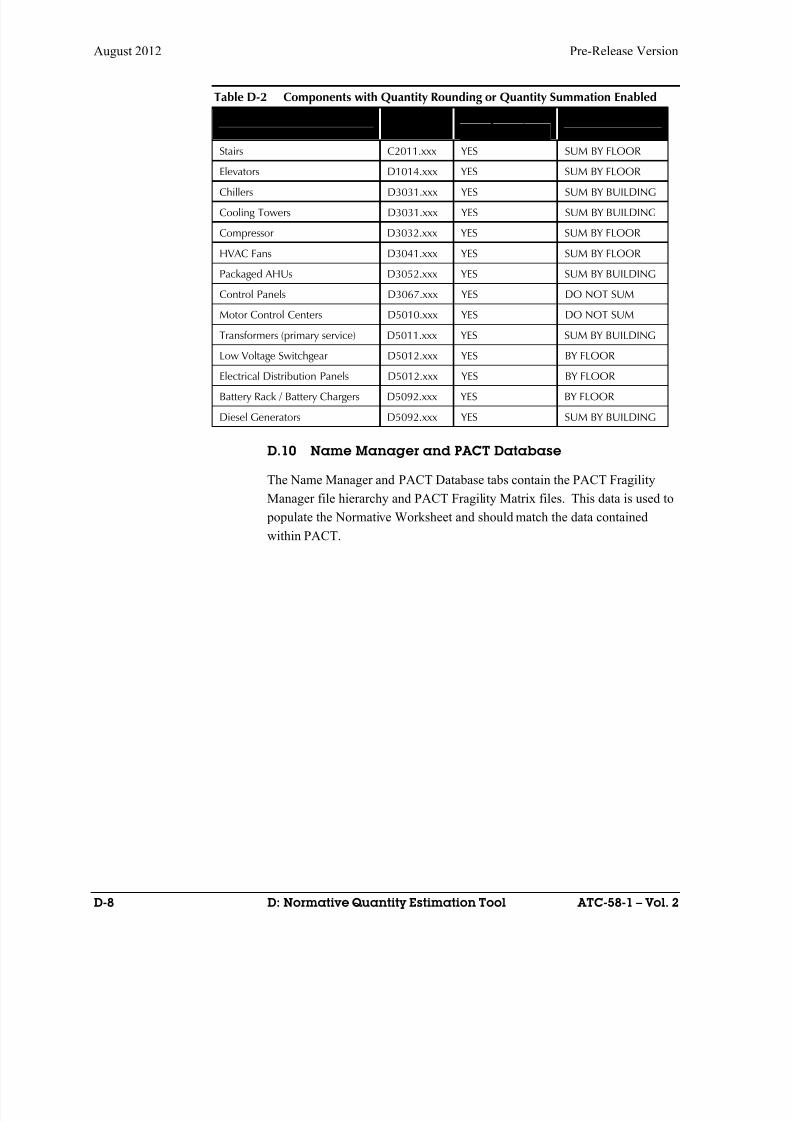
8/12/2019 Seismic Performance Assessment of Buildings
http://slidepdf.com/reader/full/seismic-performance-assessment-of-buildings 350/358
August 2012 Pre-Release Version
D-8 D: Normative Quantity Estimation Tool ATC-58-1 – Vol. 2
Table D-2 Components with Quantity Rounding or Quantity Summation Enabled
Component NISTIRNumber
QuantityRounding
Sum Component by
Stairs C2011.xxx YES SUM BY FLOOR
Elevators D1014.xxx YES SUM BY FLOOR
Chillers D3031.xxx YES SUM BY BUILDING
Cooling Towers D3031.xxx YES SUM BY BUILDING
Compressor D3032.xxx YES SUM BY FLOOR
HVAC Fans D3041.xxx YES SUM BY FLOOR
Packaged AHUs D3052.xxx YES SUM BY BUILDING
Control Panels D3067.xxx YES DO NOT SUM
Motor Control Centers D5010.xxx YES DO NOT SUM
Transformers (primary service) D5011.xxx YES SUM BY BUILDING
Low Voltage Switchgear D5012.xxx YES BY FLOOR
Electrical Distribution Panels D5012.xxx YES BY FLOOR
Battery Rack / Battery Chargers D5092.xxx YES BY FLOOR
Diesel Generators D5092.xxx YES SUM BY BUILDING
D.10 Name Manager and PACT Database
The Name Manager and PACT Database tabs contain the PACT Fragility
Manager file hierarchy and PACT Fragility Matrix files. This data is used to
populate the Normative Worksheet and should match the data contained
within PACT.
8/12/2019 Seismic Performance Assessment of Buildings
http://slidepdf.com/reader/full/seismic-performance-assessment-of-buildings 351/358
Pre-Release Version August 2012
FEMA P-58 – Vol. 2 References E-1
References
ACI, 2005, Building Code Requirements for Structural Concrete and
Commentary, ACI 318-05, American Concrete Institute, Farmington
Hills, Michigan.
ACI, 2008, Building Code Requirements for Masonry Structures and
Specifications for Masonry Structures, ACI-530-08/ ASCE 5-08/TMS
402-08, Masonry Standards Joint Committee of American Concrete
Institute, American Society of Civil Engineers, and The Masonry
Society, Farmington Hills, Michigan.
ACI, 2011, Building Code Requirements for Structural Concrete andCommentary, ACI 318-11, American Concrete Institute, Farmington
Hills, Michigan.
AF&PA, 2005a, National Design Specification for Wood Construction,
ANSI/AF&PA NDS-2005, American Forest & Paper Products
Association, Washington, D.C.
AF&PA, 2005b, Special Design Provisions for Wind and Seismic,
ANSI/AF&PA SDPWS-2005, American Forest & Paper Products
Association, Washington, D.C.
AISC, 2005, Seismic Provisions for Structural Steel Buildings, ANSI/AISC
341-05, American Institute of Steel Construction, Chicago, Illinois.
ASCE, 2002, Minimum Design Loads for Buildings and Other Structures,
ASCE/SEI 7-02, American Society of Civil Engineers, Reston, Virginia.
ASCE, 2005a, Minimum Design Loads for Buildings and Other Structures,
ASCE/SEI 7-05, American Society of Civil Engineers, Reston, Virginia.
ASCE, 2005b, Seismic Design Criteria for Structures, Systems, and
Components in Nuclear Facilities, ASCE/SEI 43-05, American Society
of Civil Engineers, Reston, Virginia.
ASCE, 2007, Seismic Rehabilitation of Existing Buildings, ASCE/SEI 41-06,
American Society of Civil Engineers, Reston, Virginia.
ASCE, 2010, Minimum Design Loads for Buildings and Other Structures,
ASCE/SEI 7-10, American Society of Civil Engineers, Reston, Virginia.

8/12/2019 Seismic Performance Assessment of Buildings
http://slidepdf.com/reader/full/seismic-performance-assessment-of-buildings 352/358
August 2012 Pre-Release Version
E-2 References ATC-58-1 – Vol. 2
ASME, 1981, Safety Code for Elevators and Escalators, ASME A17.1,
American Society of Mechanical Engineers, New York, New York.
FEMA, 2005, Improvement of Nonlinear Static Seismic Analysis Procedures,
FEMA 440, Prepared by Applied Technology Council for Federal
Emergency Management Agency, Washington, D.C.
ICC, 1994, 1997, Uniform Building Code 1994, International Code Council,
Washington, D.C.
ICC, 2000, 2009, 2012, International Building Code, International Code
Council, Washington, D.C.
Kafali, C., Fathali, S., Grigoriu, M., and Whittaker, A.S., 2007, Static and
Kinetic Coefficients of Friction for Rigid Blocks, Technical Report
MCEER-07-001, Multidisciplinary Center for Earthquake Engineering
Research, Buffalo, New York.
Lehman, D., Roeder, C.W., Herman, D., Johnson, S., and Kotulka, B., 2008,
“Improved seismic performance of gusset plate connections,” Journal of
Structural Engineering , Vol. 134, Issue 6, pp. 890-901.
Newmark, N.M., and Hall, W.J., 1982, Earthquake Design and Spectra,
Earthquake Engineering Research Institute, Oakland, California.
NFPA, 2007, Standard for Installation of Sprinkler Systems. NFPA 13,
National Fire Protection Association, Quincy, Massachusetts.
NIST, 1999, UNIFORMAT II Elemental Classification for Building
Specifications, Cost Estimating and Cost Analysis, NISTIR 6389 Report,
National Institute of Standards and Technology, Gaithersburg, Maryland.
Selna, L.G., 1981, “Slender wall tests instrumentation and results,”
Proceedings of the 50th SEAOC Convention, Coronado, California.
Tissel, J.R., 1967, 1966 Horizontal Plywood Diaphragm Tests, APA
Laboratory Report 106, American Plywood Association, Tacoma,
Washington.
Vamvatsikos, D., and Cornell, C.A., 2006, “Direct estimation of the seismic
demand and capacity of oscillators with multi-linear static pushovers
through IDA,” Earthquake Engineering and Structural Dynamics, Vol.
35, Issue 9, pp. 1097-1117.

8/12/2019 Seismic Performance Assessment of Buildings
http://slidepdf.com/reader/full/seismic-performance-assessment-of-buildings 353/358
Pre-Release Version August 2012
FEMA P-58 – Vol. 2 Project Participants F-1
Project Participants
ATC Management and Oversight
Christopher Rojahn (Project Executive Director)
Project Executive Director
Applied Technology Council
201 Redwood Shores Parkway, Suite 240
Redwood City, California 94065
Jon A. Heintz (Project Manager)
Applied Technology Council
201 Redwood Shores Parkway, Suite 240
Redwood City, California 94065
Ayse Hortacsu
Applied Technology Council
201 Redwood Shores Parkway, Suite 240
Redwood City, California 94065
FEMA Oversight
Mike Mahoney (Project Officer)
Federal Emergency Management Agency
500 C Street, SW, Room 416
Washington, DC 20472
Robert D. Hanson (Technical Monitor)
Federal Emergency Management Agency
2926 Saklan Indian Drive
Walnut Creek, California 94595
Project Management Committee
Ronald O. Hamburger
(Project Technical Director)
Simpson Gumpertz & Heger
The Landmark @ One Market, Suite 600San Francisco, California 94105
John Gillengerten
Office of Statewide Health
Planning and Development
1600 9th Street, Room 420
Sacramento, California 95814
William T. Holmes (ex-officio)
Rutherford & Chekene
55 Second Street, Suite 600
San Francisco, California 94105
Peter J. May
University of Washington
3630 Evergreen Point Road
Medina, Washington 98039
Jack P. Moehle
University of California, Berkeley
3444 Echo Springs Road
Lafayette, California 94549
Maryann T. Phipps (ATC Board Contact)
Estructure
8331 Kent Court, Suite 100
El Cerrito, California 94530

8/12/2019 Seismic Performance Assessment of Buildings
http://slidepdf.com/reader/full/seismic-performance-assessment-of-buildings 354/358
August 2012 Pre-Release Version
F-2 Project Participants FEMA P-58 – Vol. 2
Steering Committee
William T. Holmes (Chair)
Rutherford & Chekene
55 Second Street, Suite 600
San Francisco, California 94105
Roger D. Borcherdt
U.S. Geological Survey
345 Middlefield Road, MS977
Menlo Park, California 94025
Anne Bostrom
University of Washington
Parrington Hall, Room 327
Seattle, Washington 98195
Bruce Burr
Burr & Cole Consulting Engineers3485 Poplar Avenue, Suite 200
Memphis, Tennessee 38111
Kelly Cobeen
Wiss, Janney, Elstner Associates, Inc.
2200 Powell Street, Suite 925
Emeryville, California 94608
Anthony B. Court
A.B. Court & Associates
4340 Hawk Street
San Diego, California 92103
Terry Dooley
Morley Builders
2901 28th Street, Suite 100
Santa Monica, California 90405
Dan Gramer
Turner Construction Company
830 4th Avenue South, Suite 400
Seattle, Washington 98134
Michael Griffin
CCS Group, Inc.
1415 Elbridge Payne Road, Suite 265
Chesterfield, Missouri 63017
R. Jay Love
Degenkolb Engineers
300 Frank H Ogawa Plaza, Suite 450
Oakland, California 94612
David Mar
Tipping-Mar & Associates1906 Shattuck Avenue
Berkeley, California 94704
Steven McCabe
National Institute of Standards and Technology
100 Bureau Drive, MS 8630
Gaithersburg, Maryland 20899
Brian J. Meacham
Worcester Polytechnic Institute
Dept. of Fire Protection Engineering
100 Institute Road
Worcester, Massachusetts 01609
William J. Petak
University of Southern California
School of Policy Planning and Development
MC 0626
Los Angeles, California 90089
8/12/2019 Seismic Performance Assessment of Buildings
http://slidepdf.com/reader/full/seismic-performance-assessment-of-buildings 355/358
Pre-Release Version August 2012
FEMA P-58 – Vol. 2 Project Participants F-3
Risk Management Products Team John D. Hooper (Co-Team Leader)
Magnusson Klemencic Associates1301 Fifth Avenue, Suite 3200
Seattle, Washington 98101
Craig D. Comartin (Co-Team Leader)
Comartin Engineers7683 Andrea Avenue
Stockton, California 95207
Mary Comerio
University of California, Berkeley
Dept. of Architecture
232 Wurster Hall
Berkeley, California 94720
Allin Cornell (deceased)Stanford University
110 Coquito Way
Portola Valley, California 94028
Mahmoud Hachem
Degenkolb Engineers
1300 Clay Street
Oakland, California 94612
Gee Heckscher
Architectural Resources Group
1301 53rd StPort Townsend, Washington 98368
Judith Mitrani-Reiser
Johns Hopkins UniversityDept. of Civil Engineering
3400 N. Charles St., Latrobe 109
Baltimore, Maryland 21218
Peter MorrisDavis Langdon
1331 Garden Highway, Suite 310
Sacramento, California 95833
Farzad NaeimJohn A. Martin and Associates, Inc.950 S. Grand Ave., 4th FloorLos Angeles, California 90015
Keith PorterUniversity of Colorado
Dept. of Civil, Environmental, and Architectural
Engineering
Engineering Center Office Tower 428
1111 Engineering Drive
Boulder, Colorado 80309
Hope Seligson
MMI Engineering
2100 Main Street, Suite 150Huntington Beach, California 92648
Risk Management Products Consultants
Travis Chrupalo
2 Lanai Court
Chico, California 95973
D. Jared DeBock
University of Colorado
939 Cedwick Drive
Lafayette, Colorado 80026
Armen Der Kiureghian
ADK & Associates
1974 18th Avenue
San Francisco, California 94116
Scott Hagie
John A. Martin & Associates, Inc.
950 South Grand Avenue
Los Angeles, California 90015
Curt B. Haselton
California State University, Chico
Dept. of Civil Engineering
209F Langdon Hall
Chico, California 95929
Russell Larsen
Magnusson Klemencic Associates
1301 Fifth Avenue, Suite 3200
Seattle, Washington 98101

8/12/2019 Seismic Performance Assessment of Buildings
http://slidepdf.com/reader/full/seismic-performance-assessment-of-buildings 356/358
August 2012 Pre-Release Version
F-4 Project Participants FEMA P-58 – Vol. 2
Juan Murcia-Delso
University of California, San Diego
Dept. of Structural Engineering
409 University Center
9500 Gilman Drive – MC0085
La Jolla, California 92093
Scott Shell
Esherick Homsey Dodge & Davis Architects500 Treat Avenue, Suite 201
San Francisco, California 94110
P. Benson Shing
University of California, San Diego
Dept. of Structural Engineering
409 University Center
9500 Gilman Drive – MC0085
La Jolla, California 92093
Farzin Zareian
University of California, Irvine
Dept. of Civil and Environmental Engineering
Irvine, California 92697
Structural Performance Products Team Andrew S. Whittaker (Team Leader)
University at Buffalo
Dept. of Civil Engineering
230 Ketter Hall
Buffalo, New York 14260
Gregory Deierlein
Stanford University
Dept. of Civil & Environmental Engineering
240 Terman Engineering Center
Stanford, California 94305
John D. Hooper
Magnusson Klemencic Associates
1301 Fifth Avenue, Suite 3200
Seattle, Washington 98101
Yin-Nan Huang127 Paramount PkwyBuffalo, New York 14223
Laura LowesUniversity of Washington
Dept. of Civil and Environmental EngineeringBox 352700
Seattle, Washington 98195
Nicolas Luco
U. S. Geological SurveyBox 25046 – DFC – MS 966
Denver, Colorado 80225
Andrew T. Merovich
A. T. Merovich & Associates, Inc.
1950 Addison Street, Suite 205
Berkeley, California 94704
Structural Performance Products Consultants
Jack Baker
Stanford University
Dept. of Civil & Environmental Engineering
240 Terman Engineering Center
Stanford, California 94305
Dhiman Basu
University at BuffaloDept. of Civil Engineering
230 Ketter Hall
Buffalo, New York 14260
J. Daniel Dolan
Washington State University
Dept. of Civil and Environmental Engineering
405 Spokane Street, Sloan 101
P.O. Box 642910
Pullman, Washington 99164
Charles Ekiert12 Hillcrest Drive
Hamlin, New York 14464
8/12/2019 Seismic Performance Assessment of Buildings
http://slidepdf.com/reader/full/seismic-performance-assessment-of-buildings 357/358
Pre-Release Version August 2012
FEMA P-58 – Vol. 2 Project Participants F-5
Andre Filiatrault
Multidisciplinary Center for Earthquake
Engineering Research, University at Buffalo
105 Red Jacket Quadrangle
Buffalo, New York 14261
Aysegul GogusUniversity of California, Los Angeles
Dept. of Civil EngineeringLos Angeles, California 90095
Kerem Gulec
University at Buffalo
Dept. of Civil EngineeringBuffalo, New York 14260
Dawn Lehman
University of Washington
Dept. of Civil and Environmental Engineering214B More Hall
Seattle, Washington 98195
Jingjuan Li
4747 30th Avenue NE B118
Seattle, Washington 98105
Eric Lumpkin
6353 NE Radford Drive, Apt. #3917
Seattle, Washington 98115
Juan Murcia-DelsoUniversity of California, San Diego
Dept. of Structural Engineering
409 University Center
9500 Gilman Drive – MC0085
La Jolla, California 92093
Hussein Okail
University of California, San Diego
Dept. of Structural Engineering
409 University Center
9500 Gilman Drive – MC0085
La Jolla, California 92093
Charles Roeder
University of Washington
Dept. of Civil and Environmental Engineering
233B More Hall
Seattle, Washington 98195
P. Benson ShingUniversity of California, San DiegoDept. of Structural Engineering409 University Center9500 Gilman Drive – MC0085
La Jolla, California 92093
Christopher Smith
Stanford University
Dept. of Civil Engineering
MC:4020, Building 540
Stanford, California 94305
Victor Victorsson
1742 Sand Hill Road, Apt. 308
Palo Alto, California 94304
John WallaceUniversity of California, Los Angeles
Dept. of Civil Engineering
5731 Boelter Hall
Los Angeles, California 90095
Nonstructural Performance Products Team
Robert E. Bachman (Team Leader)
RE Bachman Consulting
25152 La Estrada Drive
Laguna Niguel, California 92677
Philip J. Caldwell
Schneider Electric
7 Sleepy Hollow Lane
Six Mile, South Carolina 29682
Andre Filiatrault
Multidisciplinary Center for Earthquake
Engineering Research, University at Buffalo
105 Red Jacket Quadrangle
Buffalo, New York 14261
Robert P. Kennedy
RPK Structural Mechanics Consulting, Inc.
28625 Mountain Meadow Road
Escondido, California 92026

8/12/2019 Seismic Performance Assessment of Buildings
http://slidepdf.com/reader/full/seismic-performance-assessment-of-buildings 358/358
August 2012 Pre-Release Version
Helmut Krawinkler (deceased)
Stanford University
Dept. of Civil & Environmental Engineering
240 Terman Engineering Center
Stanford, California 94305
Manos MaragakisUniversity of Nevada, Reno
Dept. of Civil EngineeringMail Stop 258
Reno, Nevada 89557
Eduardo Miranda
Stanford UniversityDept. of Civil & Environmental Engineering
Terman Room 293
Stanford, California 94305
Gilberto Mosqueda
University at Buffalo
Dept. of Civil, Structural, and Environmental
Engineering
Buffalo, New York 14260
Keith PorterUniversity of Colorado
Dept. of Civil, Environmental, and Architectural
Engineering
Engineering Center Office Tower 428
1111 Engineering Drive
Boulder, Colorado 80309
Nonstructural Performance Products Consultants
Richard Behr
Pennsylvania State University
Dept. of Architectural Engineering
104 Engineering Unit A
University Park, Pennsylvania 16802
John EidingerG&E Engineering SystemsPO Box 3592Olympic Valley, California 96146
Gregory S. HardySimpson Gumpertz & Heger
4000 MacArthur Blvd. Suite 710
Newport Beach, California 92660
Christopher Higgins
Oregon State University
220 Owen Hall
Corvallis, Oregon 97333
Gayle S. Johnson
Halcrow
500 12th Street, Suite 310Oakland, California 94607
Paul Kremer430 Canterbury Drive
State College, Pennsylvania 16802
David L. McCormick
Simpson Gumpertz & Heger
The Landmark @ One Market, Suite 600
San Francisco, California 94105
Ali M. Memari
Pennsylvania State University
104 Engineering Unit A
University Park, Pennsylvania 16802
William O'Brien The Pointe
501 Vairo Boulevard
State College, Pennsylvania 16803
John OsteraasExponent149 Commonwealth DriveMenlo Park, California 94025
Xin Xu7 Xibei Xincun, Room 403
Wuxi, Jiangsu 214062, P.R.China