seismic inversion and avo analysis applied to predictive ... inversion-avo.pdf · lain eia 936 the...

L a t i n A m e r i c a

936 The Leading Edge July 2014

SPECIAL SECTION: L at i n A m e r i c a

Seismic inversion and AVO analysis applied to predictive-modeling gas-condensate sands for exploration and early production in the Lower Magdalena Basin, Colombia

AbstractThe Plato Depression in the Lower Magdalena Basin is

a Miocene depocenter where a thick, shale-prone marine se-quence known as the Porquero Formation was laid down in basin-floor conditions. Seismic inversion carried out on new and existing 2D seismic data helped to focus early explora-tion on a shallow stratigraphic gas-sand play associated with what seemed to be isolated shale diapirs with shallow roots. A subsequent land 3D survey helped to locate the first explor-atory well, which resulted in the discovery of the Guama gas-condensate field. The main reservoir consists of laminar, low-permeability sands in a relatively thick shale-prone sequence of Early and Middle Miocene age. Sequential application of acoustic and elastic inversion and AVO analysis was used to build an evolving 3D predictive model of gas sands, extracted from an otherwise featureless seismic cube. Workflows were based on careful rock-physics analysis, simultaneous seismic inversion, and AVA analysis supported by custom well-log and seismic-gather conditioning. Work routines carried out in parallel became essential to applying quality control and fine-tuning the model, which supported three additional suc-cessful wells, early reservoir planning, and key volumetrics.

IntroductionThe Plato Depression is a deep Miocene depocenter in

the eastern Lower Magdalena Basin, in northwest Colombia. Previous exploration was aimed at deep turbiditic sands in the thick Porquero sequence of massive shales and muds in large fault blocks defined from conventional 2D seismic lines of various vintages. In 1975–1980, two wildcat wells flowed gas and condensate at rates that were consid-ered noncommercial for the depths involved (more than 10,000 ft).

In 2008, 256 km2 of 2D seismic was acquired to better define the play. A first acoustic inversion was carried in 2010 on five of the new 2D lines, where the Poisson’s ra-tio–based shaliness showed that the deep sands had limited extension. In 2010, a 3D survey was acquired over 100 km2. Interpretation of this survey improved the maps of the deeper targets and showed an addi-tional sand play at shallower depths (less than 7000 ft), making explora-tion more attractive. However, the

Mario Di Luca, Trino SaLinaS, Juan F. arMinio, and GabrieL aLvarez, Pacific Rubiales EnergyPeDro aLvarez, FranciSco boLivar, and WiLLiaM Marín, Rock Solid Images

new seismic image was still insufficient to define individual targets, dispersed as the sands are in more than 4000 ft of shales. Therefore, reservoir presence continued to be the main geologic uncertainty of the play.

AVA analysis indicated gas prospectivity for the shallow play. The first well was drilled in 2010 on the flank of one

Figure 1. Map of 3D seismic and well used in the study.

Figure 2. (a) Core photograph and (b) photomicrography of a core section, Well P-1. The photo-graphs show thin, shaley sand bands in otherwise massive, organic-rich shales. After Leyva et al., 2012, Figures 5 and 6. Used by permission.

July 2014 The Leading Edge 937

L a t i n A m e r i c a L a t i n A m e r i c a

unconformity levels. Both images highlight the main target section.

It must be emphasized here that gas charge is pervasive in the whole Porquero section, even at shallow depths.

of two shale diapirs interpreted from the new data. The well resulted in the first gas-condensate discovery in the shallow Porquero play. Cores showed that the reservoir was made of laminar, thin to medium lithic sands with fair porosity but low permeabilities.

Production tests in the different wells of the area have been done in intervals with a high percentage of laminated sandstone (1 to 4 cm). The aim of this work is to present a workflow to characterize the reservoir considering the high heterogeneity and wide range of petrophysical properties in the Porquero Formation. Seismic resolution is not enough to resolve these thin laminated sandstone intervals. However, the play can be defined by an important number of layers arranged in thick intervals interbedded in the massive shales of the Porquero Formation. The seismic data have enough resolution power to resolve the thick intervals.

The data set used in analysis of the study area consists of a 3D seismic cube and log data from five wells, as shown in Figure 1.

Geologic frameworkThe Miocene Porquero Formation in the Plato region ex-

ceeds 10,000 ft of total thickness of massive shales and silty shales with subordinated laminated shaley sands and silts. This massive shale-prone marine sequence represents slope and basin-floor settings (Arminio et al., 2011; Ghosh, 2013).

The sandstones show individual laminated bed thickness ranging from 1 to 4 cm, grouped in multiple cycles. For prac-tical purposes, the Porquero Formation has been subdivided into informal units defined between unconformities. The prospective sand cycles are contained mostly in the Porquero “C” and “D” units with a joint thickness of 2000 to 3000 ft.

The sands range in grain size from fine to medium and show complex mineralogy with abundant clay minerals (Ley-va et al., 2012). Low sand permeabilities were estimated from production tests and were measured in core samples, with values ranging from 1 mD to as low as a few nanodarcies. Figure 2 shows a well core and a thin section taken from Well P-1 at target level.

The dominant structural style is high-angle normal faults, some of which show moderate tectonic inversion. The presence of at least one shale diapir was first interpreted from 2D seismic by previous explor-ers (Arminio et al., 2011), and two of them were mapped on the 2010 3D cube. Initially considered as in-cipient features, they are now inter-preted as Miocene to Early Pliocene features, fossilized under the thin Quaternary alluvium, lacking ob-servable surface expression.

Figure 3 shows a well-log type at the study area and a section that illustrates the seismic expression of the mud diapirs and the different

Figure 3. (a) Section with seismic expression of mud diapirs and different unconformity levels. (b) Well-log type in the study area and its correlation with seismic information.

Figure 4. AVO effect in one of the target intervals at the P-1 well.



AVA and elastic inversionAs previously mentioned, the seismic resolution was not

enough to resolve individual sand beds, and the elastic-inver-sion workflow was designed to spot multisand intervals em-bedded in the massive shales.

Basic tools used in the exploration phases of this play were

• amplitude-variation-with-angle (AVA) analysis• seismic-inversion analysis supported by a rock-physics

framework

Given the presence of gas, the apparent decrease in acoustic impedance and density values at the target level afford an oppor-tunity to map sweet spots based on changes in seismic-attribute responses by an integrated rock-physics interpretation approach.

The fundamental interpretation strategy was the use of seismic attributes from AVA analysis to confirm the results of the simultaneous inversion. In case of discrepancies, detailed revisiting of well-log analysis was performed, along with a careful evaluation of seismic gathers to explain and reconcile the differences. Sometimes subtle editing of sonic logs based on rock-physics models enhanced the consistency of seismic attributes significantly.

In Figure 4, we can see the AVO effect of one of these target intervals and the graphical petrophysical evaluation of the P-1 well.

Data conditioningSeismic data. Two-dimensional and 3D seismic followed

a standard processing sequence up to prestack time migra-tion (PSTM) constrained by relative amplitude-preserving requirements. However, reservoir characterization based on quantitative seismic inter-pretation requires the data (seismic and well log) to fulfill quality-con-trol standards. Before any attempt to perform inversion, the PSTM seis-mic gathers went into an additional sequence of data-conditioning steps to enhance signal-to-noise ratio, re-cover offset-dependent frequency loss caused by NMO stretch, and align reflections with a static-based technique (Singleton, 2009).

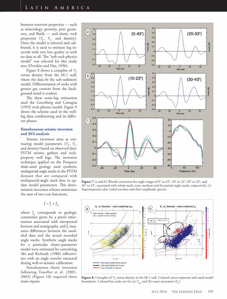
Figures 5 and 6 show some re-sults of seismic data conditioning at the gather and stack levels. This ap-proach results in more stable seismic wavelets and consistently lower lev-els of seismic-inversion residuals, as shown in Figure 7.

Well-log data. Along with seismic data, well logs were also conditioned. Normally, well-log analysis focuses on the target level of interest. Howev-er, for inversion purposes, the whole column needs to be conditioned to edit and reconstruct a complete and reliable set of well logs. Sonic logs in particular are used to generate syn-thetic seismograms in the seismic well-calibration process. This condi-tioning workflow includes volumet-ric estimation, rock-physics analysis, fluid substitution, multiwell analysis, prestack synthetic seismograms, and well-log AVO analysis.

Rock-physics analysis results in a theoretical model that best explains the behavior of the measured well-log data. This model is the link

Figure 6. Seismic data conditioning, carried out on partial-angle stacks for a range of 20° to 33°: (a) input stack; (b) stack after noise attenuation (NA); (c) stack after NA, alignment, and NMO stretch compensation.

Figure 5. Seismic gather conditioning: (a) input; (b) output; (c) residual.



between reservoir properties — such as mineralogy, porosity, pore geom-etry, and fluids — and elastic rock properties (VP, VS , and density). Once the model is selected and cali-brated, it is used to estimate log in-tervals with very low quality or with no data at all. The “soft rock-physics model” was selected for this study area (Dvorkin and Nur, 1996).

Figure 8 shows a crossplot of VP versus density from the M-1 well, where the data fit the soft-sediment model. Differentiation of rocks with greater gas content from the back-ground trend is evident.

The shear sonic-log estimation used the Greenberg and Castagna (1992) rock-physics model. Figure 9 shows the scheme used in the well-log data conditioning and its differ-ent phases.

Simultaneous seismic inversion and AVA analysis

Seismic inversion aims at esti-mating model parameters (VP , VS , and density) based on observed data: PSTM seismic gathers and rock-property well logs. The inversion technique applied on the Porquero shale-sand geology used synthetic multipartial-angle stacks in the PSTM domain that are compared with multi partial-angle stack data to up-date model parameters. This deter-ministic inversion scheme minimizes the sum of two cost functions,

J = Js + Jg,

where Jg corresponds to geologic constraints given by a priori infor-mation associated with interpreted horizon and stratigraphy, and Js mea-sures differences between the mod-eled data and the actual recorded angle stacks. Synthetic angle stacks for a particular elastic-parameter model were estimated by convolving Aki and Richards (1980) reflectivi-ties with an angle wavelet extracted during well-to-seismic calibration.

Simultaneous elastic inversion fol low ing Tonellot et al. (2001, 2002) (Figure 10) required three main inputs:

Figure 7. (a and b) Wavelet extraction for angle ranges of 0° to 43°, 10° to 23°, 20° to 33°, and 30° to 43°, associated with whole-stack, near, medium and far partial-angle stacks, respectively. (c) Superimposed color-coded wavelets and their amplitude spectra.

Figure 8. Crossplot of VP versus density in the M-1 well. Colored curves represent soft-sand-model boundaries. Colored bar scales are for (a) Vclay and (b) water saturation (Sw).



• elastic-property initial models (VP, VS, and density)

• partial incident-angle stacks• extracted seismic wavelets

The model parameters are based on well logs from five wells and on seismic markers interpreted at dif-ferent stratigraphic levels. The ini-tial model structure for the elastic parameters was low-pass-filtered to obtain a 3D regional trend for the much higher-frequency inversion outcome.

The ranges of the selected par-tial-angle stacks were 0° to 13°, 10° to 23°, and 20° to 33°, associated with near, medium, and far offsets, respectively. Figure 11 shows an in-put partial stack, a modeled stack, and an inversion residual section for an angle range of 10° to 23°.

Quantitative interpretation — Rock-physics analysis

Crossplots were generated from log-derived elastic properties. From them, elastic facies were interpreted in the wells. Figure 12 shows two of the crossplots obtained from this analysis, with a large overlap in the impedance axis. Because of the overlap, discrimi-nating lithology and fluid proved to be difficult. In the Poisson’s ratio axis, however, we found that over the tar-get section (higher IP), the cleanest rocks (lower Vclay values) show lower Poisson values.

Figure 12. Crossplot of Poisson’s ratio versus IP for the M-1 well. Sample points are color-coded for (a) Vclay and (b) Sw. In part (a), black and gray represent higher Vclay values, in contrast with brown and orange, which represent lower Vshale values. In part (b), blues represents higher Sw values and red lower Sw. Cleaner sands tend to show lower Poisson’s ratio values.

Figure 9. Well-log data-conditioning workflow: volumetric estima-tion, rock-physics analysis, fluid substitution, multiwell analysis, prestack synthetic seismogram, and well-log AVO analysis.

Figure 11. Seismic-inversion quality control: (a) observed partial-angle stack; (b) modeled partial-angle stack; (c) inversion residual section for angle range of 10° to 23°.

Figure 10. Simultaneous elastic-seismic workflow applied on the Porquero succession of massive shale and thin sand.



Similarly, Figure 13 shows a crossplot of VP versus VS for the M-1 well, in which we can see that higher values of VP and VS are associated with target intervals.

The next step was a fluid-sub-stitution model, using the Biot-Gassmann equations (Mavko et al., 1998). Because of limitations in log data in the older well, the analysis was done on only four wells.

The fluid-substitution study in-cor porated the in situ state and cases with water saturations of 40%, 60%, and 100%. All the scenarios used fluid parameters as measured on the wells: gas gravity 0.62, con-densate API gravity 50°, and water salinity 25,000 ppm.

Figure 14 shows a profile of den-sity, VP and VS logs, P-impedance, and Poisson’s ratio for the indicated values of fluid substitution in the K-1 well. Black curves represent the in situ base case. In Figure 15, analy-sis of the crossplot of Poisson’s ratio versus IP from the K-1 well shows a clear separation between samples from partially gas-saturated and 100% water-saturated rocks. There is, however, no significant separation between samples with water satura-tion of 40% and 60%.

Reservoir identification and lithologic maps

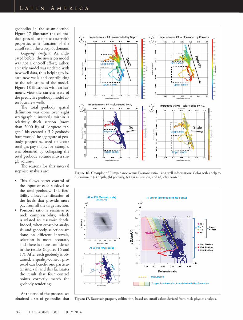
The crossplot of P-impedance (IP) versus Poisson’s was chosen as the parameter that best discrimi-nates gas-sand-prone sections. Fig-ure 16 shows four crossplots based on well-log data that illustrate values of IP and Poisson’s ratio that repre-sent good reservoir properties. The four crossplots were used to define prospective zones (indeed, 3D geo-body renderings, rather than indi-vidual reservoir layers that are im-possible to discriminate) and their associated porosity, gas saturation, and clay content.

By combining the crossplots with calibration of seismic inver-sion obtained from the 3D seismic cube, it was possible to define the most prospective sections in the 3D seismic area by defining distributed

Figure 13. Crossplot of VP versus VS of the M-1 well. Sample points are color-coded for (a) Vclay and (b) Sw. In part (a), black and gray represent higher Vclay values, in contrast with brown and orange, which represent lower Vshale values. In part (b), blues represents higher Sw values and red lower Sw. Rocks with lower Sw tend to have higher VS values in the target section.

Figure 14. Density, VP, and VS logs, IP, and Poisson’s ratio for different cases of fluid substitution in the K-1 well. Black curves correspond to the in situ case.

Figure 15. Crossplot of Poisson’s ratio versus IP for three cases of fluid substitution in the K-1 well.



geobodies in the seismic cube. Figure 17 illustrates the calibra-tion procedure of the reservoir’s properties as a function of the cutoff set in the crossplot domain.

Ongoing analysis. As indi-cated before, the inversion model was not a one-off effort; rather, an early model was updated with new well data, thus helping to lo-cate new wells and contributing to the robustness of the model. Figure 18 illustrates with an iso-metric view the current state of the predictive geobody model af-ter four new wells.

The total geobody spatial definition was done over eight stratigraphic intervals within a relatively thick section (more than 2000 ft) of Porquero tar-get. This created a 3D geobody framework. The aggregate of geo-body properties, used to create total gas-pay maps, for example, was obtained by collapsing the total geobody volume into a sin-gle volume.

The reasons for this interval stepwise analysis are:

• This allows better control of the input of each sublevel to the total geobody. This flex-ibility allows identification of the levels that provide more pay from all the target section.

• Poisson’s ratio is sensitive to rock compressibility, which is related to reservoir depth. Indeed, when crossplot analy-sis and geobody selection are done on different intervals, selection is more accurate, and there is more confidence in the results (Figures 16 and 17). After each geobody is ob-tained, a quality-control pro-tocol can benefit one particu-lar interval, and this facilitates the result that four control points correctly match the geobody rendering.

At the end of the process, we obtained a set of geobodies that

Figure 16. Crossplot of P impedance versus Poisson’s ratio using well information. Color scales help to discriminate (a) depth, (b) porosity, (c) gas saturation, and (d) clay content.

Figure 17. Reservoir-property calibration, based on cutoff values derived from rock-physics analysis.



represents the higher probability of gas-bearing sand. The geo-body from the crossplot selection is generated in time, and then a time-depth velocity model is used to obtain a geobody thickness of each interval. As an example, Figure 19 shows the aggregate of inversion-derived total gas pay for one of eight stratigraphic subdivisions of the Porquero prospective section.

ConclusionsThe case history presented here shows the simultaneous

application of AVA and elastic inversion to predict sand pres-ence and gas saturation in massive shales, in this case, a very thick Miocene section where 3D seismic images are insuffi-cient to discriminate individual reservoir horizons.

On finishing a first exploration in the area, several ele-ments can be deemed relevant to four successful wells:

• Definition of several stratigraphic work subunits helped to focus analysis of the otherwise thick and massive suc-cession.

• Acquisition of log suites for each well, including dipolar and borehole imaging, helped to build an early, robust rock-physics model that could be updated as new wells were finished and tested.

• Dedicated well and seismic data conditioning helped to improve signal-to-noise ratio and enhanced accuracy and stability of results.

ReferencesAki, K., and P. G. Richards, 1980, Quantitative seismology: Theory

and methods: W. H. Freeman and Co.Arminio, J. F., F. Yoris, E. García, L. Porras, and M. Di Luca, 2011,

Petroleum geology of Colombia: Lower Magdalena Basin, v. 10, F. Cediel, ed.: Agencia Nacional de Hidrocarburos, www.anh.org, accessed 21 February 2014.

Dvorkin, J. and A. Nur, A., 1996, Elasticity of high-porosity sand-stones: Theory for two North Sea data sets: Geophysics, 61, no. 5, 559–564, http://dx.doi.org/10.1190/1.1444059.

Ghosh, S. K., M. Di Luca, V. Azuaje, J. G. Betancourt, and D. Del Pilar, 2013, Valle Inferior de Magdalena — Area Guama: Marco Estratigrafico-Sedimentológico: Pacific Rubiales Energy, internal report.

Greenberg, M. L., and J. P. Castagna, 1992, Shear-wave velocity es-timation in porous rocks: Theoretical formulation, preliminary verification and applications: Geophysical Prospecting, 40, no. 2, 195–209, http://dx.doi.org/10.1111/j.1365-2478.1992.tb00371.x.

Leyva I., J. F. Arminio, R. Vega, J. Lugo, and A. Dasilva, and J. Tavel-la, 2012, Exploración de plays no convencionales para gas en la Formación Porquero de la Cuenca del Valle Inferior del Magda-lena: Memorias del XI Simposio Bolivariano ACGGP.

Mavko, G., Mukerji, T., and Dvorkin, J., 1998, The rock physics handbook: Tools for seismic analysis in porous media: Cambridge University Press.

Singleton, S., 2009, The effects of seismic data conditioning on prestack simultaneous impedance inversion: The Leading Edge, 28, no. 7, 772–781, http://dx.doi.org/10.1190/1.3167776.

Tonellot, T., D. Macé, and V. Richard, 2001, Joint stratigraphic in-version of angle-limited stacks: 71st Annual International Meet ing,

Figure 18. 3D view showing well paths used in the analysis, Poisson’s ratio over an arbitrary section, and representative geobodies derived from seismic-inversion analysis.

Figure 19. Thickness map (in feet) of gas sand of one of the levels analyzed, showing remarkable coherence with the interpreted depositional model of basin-floor aprons and distributaries.

SEG, Expanded Abstracts, 227–230, http://dx.doi.org/10. 1190 /1. 1816577.

Tonellot, T., D. Macé, and V. Richard, 2002, 3D quantitative AVA: Joint versus sequential stratigraphic inversion of angle-limited stacks: 72nd Annual International Meeting, SEG, Expanded Ab-stracts, 253–256, http://dx.doi.org/10.1190/1.1817223..

Acknowledgments: We thank Pacific Rubiales Energy and Rock Solid Images for their authorization to publish the information presented in this article.

Corresponding author: [email protected]

seismic inversion and avo analysis applied to predictive ... inversion-avo.pdf · lain eia 936 the...

Documents