Seismic Fragility Analysis of Highway Bridges

Sponsored by

Mid-America Earthquake Center

Technical Report

MAEC RR-4 Project

Prepared by

Howard Hwang, Jing Bo Liu, and Yi-Huei Chiu

Center for Earthquake Research and Information

The University of Memphis

July 2001

ii

ABSTRACT

Past earthquakes, such as the 1971 San Fernando earthquake, the 1994 Northridge earthquake,

the 1995 Great Hanshin earthquake in Japan, and the 1999 Chi-Chi earthquake in Taiwan, have

demonstrated that bridges are vulnerable to earthquakes. The seismic vulnerability of highway

bridges is usually expressed in the form of fragility curves, which display the conditional

probability that the structural demand (structural response) caused by various levels of ground

shaking exceeds the structural capacity defined by a damage state. Fragility curves of structures

can be generated empirically and analytically. Empirical fragility curves are usually developed

based on the damage reports from past earthquakes, while analytical fragility curves are

developed from seismic response analysis of structures and the resulting fragility curves are

verified with actual earthquake data, if available. Since earthquake damage data are very scarce

in the central and eastern United States, the analytical method is the only feasible approach to

develop fragility curves for structures in this region.

This report presents an analytical method for the development of fragility curves of highway

bridges. In this method, uncertainties in the parameters used in modeling ground motion, site

conditions, and bridges are identified and quantified to establish a set of earthquake-site-bridge

samples. A nonlinear time history response analysis is performed for each earthquake-site-

bridge sample to establish the probabilistic characteristics of structural demand as a function of a

ground shaking parameter, for example, spectral acceleration or peak ground acceleration.

Furthermore, bridge damage states are defined and the probabilistic characteristics of structural

capacity corresponding to each damage state are established. Then, the conditional probabilities

that structural demand exceeds structural capacity are computed and the results are displayed as

fragility curves. The advantage of this approach is that the assessment of uncertainties in the

modeling parameters can be easily verified and refined. To illustrate the proposed method, the

method is applied to a continuous concrete bridge commonly found in the highway systems

affected by the New Madrid seismic zone.

iii

ACKNOWLEDGMENTS

The work described in this report was conducted as part of the Mid-America Earthquake (MAE)

Center RR-4 Project. This work was supported primarily by the Earthquake Engineering

Research Centers Program of the National Science Foundation under Award Number EEC-

9701785. Any opinions, findings, and conclusions expressed in the report are those of the

writers and do not necessarily reflect the views of the MAE Center, or the NSF of the United

States.

iv

TABLE OF CONTENTS

SECTION TITLE PAGE

1 INTRODUCTION 1

2 DESCRIPTION AND MODELING OF BRIDGE 3

2.1 Description of Bridge 3

2.2 Finite Element Model of Bridge 4

2.3 Modeling of Bearings 4

2.4 Modeling of Nonlinear Column Elements 5

2.5 Modeling of Pile Footings 8

2.6 Modeling of Abutments 9

3 GENERATION OF EARTHQUAKE ACCELERATION

TIME HISTORIES 28

3.1 Generation of Ground Motion at the Outcrop of a Rock Site 28

3.2 Generation of Ground Motion at the Ground Surface of a Soil Site 32

3.3 Illustration of Generation of Acceleration Time Histories 33

4 SEISMIC DAMAGE ASSESSMENT OF BRIDGE 45

4.1 Nonlinear Seismic Response Analysis of Bridge 45

4.2 Seismic Damage Assessment of Bearings 46

4.3 Seismic Damage Assessment of Columns in Shear 47

4.4 Seismic Damage Assessment of Columns in Flexure 49

4.5 Alternative Approach for Seismic Damage Assessment of Bridge 50

v

SECTION TITLE PAGE

5 UNCERTAINTIES IN THE EARTHQUAKE-SITE-BRIDGE

SYSTEM 82

5.1 Uncertainty in Earthquake Modeling 82

5.2 Uncertainties in Soil Modeling 82

5.3 Uncertainty in Bridge Modeling 84

5.4 Generation of Earthquake-Site-Bridge Samples 85

6 PROBABILISTIC SEISMIC DEMAND 101

7 SEISMIC FRAGILITY ANALYSIS OF BRIDGE 108

8 DISCUSSIONS AND CONCLUSIONS 113

9 REFERENCES 115

vi

LIST OF TABLES

TABLE TITLE PAGE

3-1 Summary of Seismic Parameters 34

4-1 Maximum Displacements Resulting From Earthquake 55

4-2 Maximum Forces at the Bottom of Columns 56

4-3 Damage Assessment Criteria for Bearings 57

4-4 Damage Assessment of Bearings 58

4-5 Determination of tanα 59

4-6 Summary of Column Shear Strength 60

4-7 Seismic Damage Assessment Criteria for Columns with Splice

in Flexure 61

4-8 Seismic Damage Assessment Criteria for Columns without Splice

in Flexure 61

4-9 Characteristic Moments and Curvatures at the Top of Columns 62

4-10 Characteristic Moments and Curvatures at the Bottom of Columns 62

4-11 Determination of p2θ 63

4-12 Determination of p4θ 64

4-13 Maximum Displacements at the Top of Columns 65

4-14 Maximum Forces at the Top of Columns 65

4-15 Maximum Displacements at the Bottom of Columns 66

4-16 Maximum Forces at the Bottom of Columns 66

4-17 Determination of Damage Status at the Top of Columns 67

vii

TABLE TITLE PAGE

4-18 Determination of Damage Status at the Bottom of Columns 68

4-19 Bridge Damage States (HAZUS99) 69

4-20 Bridge Damage States Measured by Displacement Ductility Ratios 70

5-1 Uncertainties in Seismic Parameters 86

5-2 Ten Samples of Quality Factor Parameters 87

5-3 Summary of Seismic Parameters 88

5-4 Uncertainty in Soil Parameters 90

5-5 Material Values of Ten Bridge Samples 91

5-6 Stiffness of Pile Footings 92

5-7 Spring Stiffness of Abutments 93

5-8 Earthquake-Site-Bridge Samples 94

6-1 Summary of Structural Response to Earthquakes 103

7-1 Median Structural Capacities Corresponding to Various 110

Displacement Ductility Ratios

viii

LIST OF ILLUSTRATIONS

FIGURE TITLE PAGE

2-1 Plan and Elevation of a 602-11 Bridge 12

2-2 Transverse Section of a 602-11 Bridge 13

2-3 Connection of Girders and Cap Beams 14

2-4 Detail of Abutment 15

2-5 Cross Sections of Columns and Cap Beams 16

2-6 Joint Reinforcement of Column and Cap Beam 17

2-7 Detail of Column Splice at the Bottom of Column 18

2-8 Plan of Pile Footing 19

2-9 Three Dimensional View of the Bridge Finite Element Model 20

2-10 Transverse View of the Bridge Finite Element Model 21

2-11 Shear Force-Displacement Diagram of a Bridge Bearing 22

2-12 Column Interaction Diagram of a Bridge Column Section 23

2-13 Moment-Curvature Diagram (P = 249 kips) 24

2-14 Moment-Curvature Diagram (P = 338 kips) 25

2-15 Bilinear Model of SAP200 Nonlinear Element 26

2-16 Equivalent Stiffness of Pile Footing 27

3-1 Illustration of Generating Synthetic Ground Motion 35

3-2 Shear Modulus Reduction and Damping Ratio Curves

for Sandy Layers 36

3-3 Average Effect of Confining Pressure on Shear Modulus

Reduction Curves for Sands 37

3-4 Shear Modulus Reduction and Damping Ratio Curves for

Clays with PI = 15 38

3-5 Shear Modulus Reduction and Damping Ratio Curves for

Clays with PI = 50 39

3-6 A Profile of Rock Layers 40

ix

FIGURE TITLE PAGE

3-7 Acceleration Time History at the Rock Outcrop 41

3-8 A Profile of Soil Layers 42

3-9 Acceleration Time History at the Ground Surface 43

3-10 Acceleration Response Spectrums at the Ground Surface

and Rock Outcrop 44

4-1 Fundamental Mode of the Bridge in the Transverse Direction 71

4-2 Fundamental Mode of the Bridge in the Longitudinal Direction 72

4-3 Column Numbers and Bearing Numbers 73

4-4 Displacement Time History at the Top of Column 5 74

4-5 Displacement Time History at the Bottom of Column 5 75

4-6 Moment Time History at the Bottom of Column 5 76

4-7 Shear Force Time History at the Bottom of Column 5 77

4-8 Axial Force Time History at the Bottom of Column 5 78

4-9 Relationship Between Displacement Ductility Ratio and

Column Shear Strength 79

4-10 Damage Pattern of Bent 2 80

4-11 Damage Pattern of Bent 3 81

5-1 Shear Modulus Reduction and Damping Ratio Curves

for Sand 95

5-2 Shear Modulus Reduction and Damping Ratio Curves

for Clays with PI = 15 96

5-3 Shear Modulus Reduction and Damping Ratio Curves

for Clays with PI = 50 97

5-4 Ten Samples of Shear Modulus Reduction Ratio Curve

for Clay with PI = 15 98

x

FIGURE TITLE PAGE

5-5 Ten Samples of Damping Ratio Curve for Clay with PI = 15 99

5-6 Generation of Earthquake-Site-Bridge Samples 100

6-1 Regression Analysis of Displacement Ductility Ratio Versus

Spectral Acceleration 106

6-2 Regression Analysis of Displacement Ductility Ratio Versus

Peak Ground Acceleration 107

7-1 Fragility Curves of 602-11 Bridge as a Function of

Spectral Acceleration 111

7-2 Fragility Curves of 602-11 Bridge as a Function of

Peak Ground Acceleration 112

1

SECTION 1

INTRODUCTION

Past earthquakes, such as the 1971 San Fernando earthquake, the 1994 Northridge earthquake,

the 1995 Great Hanshin earthquake in Japan, and the 1999 Chi-Chi earthquake in Taiwan, have

demonstrated that bridges are vulnerable to earthquakes. Since bridges are one of the most

critical components of highway systems, it is necessary to evaluate the seismic vulnerability of

highway bridges in order to assess economic losses caused by damage to highway systems in the

event of an earthquake. The seismic vulnerability of highway bridges is usually expressed in the

form of fragility curves, which display the conditional probability that the structural demand

(structural response) caused by various levels of ground shaking exceeds the structural capacity

defined by a damage state.

Fragility curves of bridges can be developed empirically and analytically. Empirical fragility

curves are usually developed based on the damage reports from past earthquakes (Basoz and

Kiremidjian, 1998; Shinozuka, 2000). On the other hand, analytical fragility curves are

developed from seismic response analysis of bridges, and the resulting curves are verified with

actual earthquake data, if available (Hwang and Huo; 1998; Mander and Basoz, 1999). Since

earthquake damage data are very scarce in the central and eastern United States (CEUS), the

analytical method is the only feasible approach to develop fragility curves for bridges in this

region. This report presents an analytical method for the development of fragility curves of

highway bridges.

The procedure for the seismic fragility analysis of highway bridges is briefly described as

follows:

1. Establish an appropriate model of the bridge of interest in the study.

2. Generate a set of earthquake acceleration time histories, which cover various levels of

ground shaking intensity.

3. Quantify uncertainties in the modeling seismic source, path attenuation, local site

condition, and bridge to establish a set of earthquake-site-bridge samples.

2

4. Perform a nonlinear time history response analysis for each earthquake-site-bridge

sample to simulate a set of bridge response data.

5. Perform a regression analysis of simulated response data to establish the probabilistic

characteristics of structural demand as a function of a ground shaking parameter, for

example, spectral acceleration or peak ground acceleration.

6. Define bridge damage states and establish the probabilistic characteristics of

structural capacity corresponding to each damage state.

7. Compute the conditional probabilities that structural demand exceeds structural

capacity for various levels of ground shaking.

8. Plot the fragility curves as a function of the selected ground shaking parameter.

The highway bridges affected by the New Madrid seismic zone have been collected by the Mid-

America Earthquake Center (French and Bachman, 1999). To illustrate the proposed method,

the method is applied to a continuous concrete bridge commonly found in the highway systems

affected by the New Madrid seismic zone.

3

SECTION 2

DESCRIPTION AND MODELING OF BRIDGE

2.1 Description of Bridge

The bridge selected for this study is a bridge with a continuous concrete deck supported by

concrete column bents, denoted as a 602-11 bridge according to the bridge classification system

established by Hwang et al. (1999). As shown in Figure 2-1, the bridge is a four span structure

with two 42.5 ft end spans and two 75 ft interior spans, and thus, the total length of the bridge is

235 ft. The superstructure of the bridge consists of a 58-ft wide, 7-in. thick, continuous cast-in-

place concrete deck supported on 11 AASHTO Type III girders spaced at 5.25 ft (Figure 2-2).

The girders are supported on reinforced concrete four-column bents. The bearing between the

girder and the cap beam of concrete column bent consists of a 1-in. Neoprene pad and two 1-in.

diameter A307 Swedge dowel bars projecting 9 in. into the cap beam and 6 in. up into the bottom

of the girder (Figure 2-3). At the ends of the bridge, the girders are supported on the abutments

(Figure 2-4). As shown in Figures 2-1 and 2-4, the abutment is an integral, open end, spill

through abutment with U-shaped wing walls. The back wall is 6 ft 10 in. in height and 58 ft in

width. The wing wall is 6 ft 10 in. in height and 9 ft 6 in. in width. The abutment is supported

on ten 14 ft × 14 ft concrete piles.

The concrete column bent consists of a 3.25 ft by 4.0 ft cap beam and four 15 ft high, 3 ft

diameter columns. The cross sections of the column and the cap beam are shown in Figure 2-5.

The vertical reinforcing bars of the column consists of 17-#7, grade 40 vertical bars extending

approximately 36 in. straight into the cap beam (Figure 2-6). The vertical bars are spliced at the

top of the footing with 17-#7 dowel bars projecting 28 in. into the column (Figure 2-7). The

dowels have 90-degree turned out from the column centerlines. The column bents are supported

on pile footings. The pile cap is 9 ft × 9 ft × 3.5 ft. The pile cap has a bottom mat of

reinforcement consisting of 19-#6 each way located 12 in. up from the bottom of the pile cap.

The pile cap has no shear reinforcement. As shown in Figure 2-8, the pile cap is supported on

eight 14 in. × 14 in. precast concrete piles. The piles spaced at 2.75 ft are reinforced with 4-#7

4

vertical bars and #2 square spirals. It is noted that the piles are embedded 12 in. into the bottom

of the pile cap and are not tied to the pile caps with reinforcing bars.

2.2 Finite Element Model of Bridge

The bridge is modeled with finite elements as described in the computer program SAP2000

(1996). A three dimensional view of the model is shown in Figure 2-9, and a transverse view of

the model is shown in Figure 2-10. The bridge deck is modeled with 4-node plane shell

elements. The girders and cap beams are modeled with beam elements. The bearings between

girders and cap beams are modeled using Nllink elements. As shown in Figure 2-10, the

corresponding nodes between deck and girder, girder and bearing, bearing and cap beam, and

cap beam and top of the column are all connected with rigid elements.

The bridge bent consists of four columns. Each column is modeled with four beam elements and

two Nllink elements placed at the top and the bottom of the column. The Nllink element is used

to simulate the nonlinear behavior of the column. The pile foundation is modeled as springs.

The abutment is modeled using beam elements supported on springs. In the following sections,

the modeling of bearings, nonlinear column elements, pile foundations, and abutments are

described in detail.

2.3 Modeling of Bearings

The bearings between girders and cap beams are modeled using Nllink elements. A Nllink

element has six independent nonlinear springs, one for each of six deformational degrees of

freedom (SAP2000, 1996). In this study, a bearing is idealized as a shear element. That is, the

stiffness of the axial spring is taken as infinite; the stiffness of torsional spring and bending

spring is taken as zero, and the stiffness of two horizontal springs is determined below.

The shear force-displacement relationship for two horizontal springs is taken as bilinear (Figure

2-11). The elastic shear stiffness provided by two 1-in. diameter A307 Swedge bolts is

determined as follows:

5

hGAKbh /= (2-1)

where G is the shear modulus of a Swedge bolt, A is the gross area of two bolts, and h is the

thickness of the Neoprene pad. Substituting G, A and h into Equation (2-1), the shear stiffness of

the bearing is determined as ftkips210132kips/in17511 ==bhK . The post-yield shear

stiffness ratio is the ratio of the post-yield shear stiffness to the elastic shear stiffness. Mander et

al. (1996) carried out an experiment to determine the characteristics of the 1-in. diameter Swedge

bolt. From their experimental results, the post yield stiffness ratio is taken as 0.3. Also from the

test results by Mander et al. (1996), the tensile yield stress of the Swedge bolt is taken as yf =

380 Mpa = 55 ksi, and the ultimate tensile stress is suf = 545 Mpa = 79 ksi. Thus, the shear

yield stress of the Swedge bolt is ysf = 3/yf = 55 3/ = 32 ksi, and the shear yield strength

of a bearing (two Swedge bolts) is kips5057.132 =×== AfV ysby . Similarly, the ultimate

shear stress of the Swedge bolt is syf = suf 3/ = 79 3/ = 46 ksi, and the ultimate shear

strength of one bearing is kips721.5746 =×== AfV svbu .

2.4 Modeling of Nonlinear Column Elements

2.4.1 Effect of Lap Splices on Column Flexural Strength

As shown in Figure 2-7, the longitudinal reinforcing bars are spliced at the bottom of the

columns. The maximum tensile force bT that can be developed in a single reinforcing bar at the

splice is (Priestley et al., 1996)

stb plfT = (2-2)

Where sl is the lap length, tf is the tension strength of the concrete, p is the perimeter of the

crack surface around a bar. For a circular column, p is determined as follows:

6

���

��� +++= )(22),(2

2'min cdcd

nDp bb

π (2-3)

where n is the number of longitudinal bars. Given in8/7=bd , in32' =D , in2=c , and

17=n , p is determined as

{ } incdcdnDp bb 13.813.8,71.8min)(22),(2

2'min ==

���

��� +++= π

In this study, tf is taken as the direct tension strength of concrete and is determined as

'4 ct ff = . Given 'cf = 4500 psi, tf is equal to 0.268 ksi.

Substituting p = 8.13 in, tf = 0.268 ksi, and in28=sl into Equation (2-2), the maximum tensile

force bT is determined as

kipsTb 612813.8268.0 =××=

Given 2in6.0=bA and ksi8.48=yf , the yield strength of a reinforcing bar is

yb fA = kips298.486.0 =×

Since bT is larger than yb fA , the yield strength of a reinforcing bar can be developed. As a

result, the ideal flexural strength of a column section with lap splices can be developed.

7

2.4.2 Moment-Curvature Relationship for a Column Section

The nonlinear characteristics of a column section are affected by the axial force acting on the

column. In this study, the axial force from dead load is used. Given the geometry of a column

section and reinforcement, the moment-curvature interaction diagram of a column section is

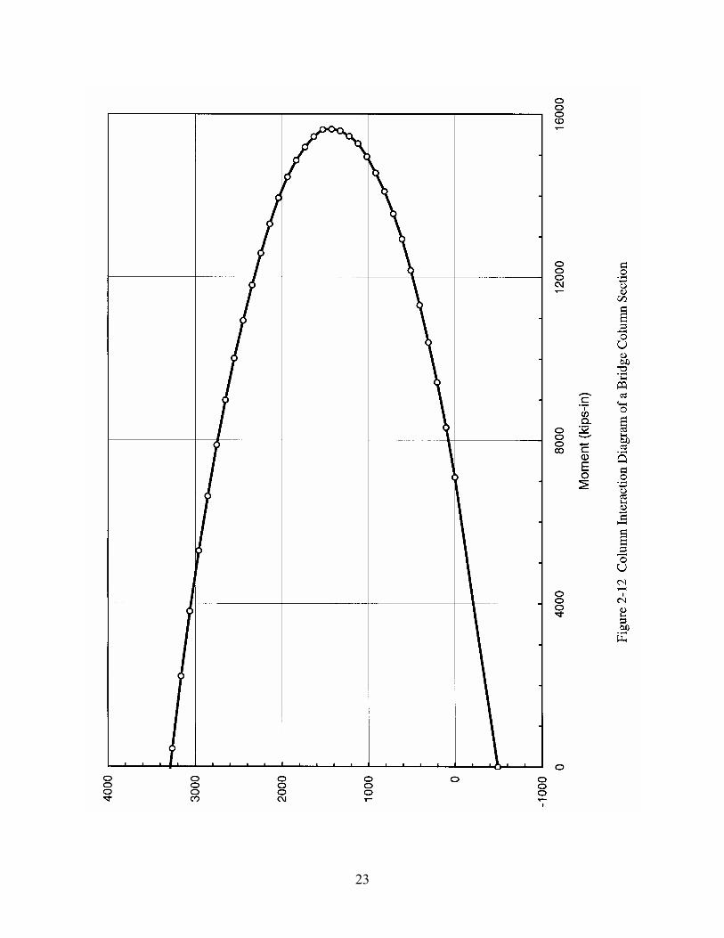
determined using the program BIAX (Wallace, 1992). Figure 2-12 shows the moment-curvature

interaction diagram for a column section with the concrete compression strain of the outer

concrete fiber cε equal to 0.004. Figures 2-13 and 2-14 show the moment-curvature relationship

for column sections with the axial force P = 249 kips and 338 kips, which correspond to the case

of the axial force being minimum and maximum. As shown in these figures, the moment-

curvature relation of a column section is idealized as elastoplastic. The idealized yield moment

yM is taken as 4M , which is the ultimate capacity of a column section with cε equal to 0.004.

The corresponding yield curvature yφ is computed as

11

φφMM y

y = (2-4)

where 1M and 1φ are the moment and curvature at the first yielding, that is, the vertical

reinforcing bars reach the steel yield strength at the first time.

2.4.3 Properties of Nonlinear Column Elements

The nonlinear behavior of a column is modeled using an Nllink element. The force-deformation

relations for axial deformation, shear deformation, and rotations are assumed to be linear. The

bending moment-deformation relationship is considered as bilinear as shown in Figure 2-15. In

this figure, K is the elastic spring constant, YIELD is the yield moment, and RATIO is the ratio of

post-yield stiffness to elastic stiffness. EXP is an exponent greater than or equal to unity, and a

larger value of EXP increases the sharpness of the curve at the yield point as shown in Figure 2-

15. The value of YIELD is equal to the yield flexural strength of a column section as described in

Section 2.4.2. The values of RATIO and EXP are taken as 0 and 10, respectively, in this study.

8

It is noted that the bilinear model is selected because of the limitation of the SAP2000 program.

In the future, other hysteretic models will be explored.

2.5 Modeling of Pile Footings

The soils surrounding the piles are taken as loose granular soils. According to ATC-32 (1996),

the lateral stiffness pk of one concrete pile in loose granular soils is kips/in20=pk and the

ultimate capacity pf of one pile is kips40=pf .

The pile foundation is modeled as springs as shown in Figure 2-16. The stiffness of springs in

the vertical direction and two rotational directions are taken as infinite. The contribution of pile

cap to the stiffness of the spring is not included, and following the suggestions by Priestly et al.

(1996), the group effect of pile foundation is also not included.

The horizontal stiffness and the ultimate capacity of the spring are derived from concrete piles as

follows:

pp knK ×= (2-5)

pp fnF ×= (2-6)

where pn is the number of piles in a pile footing. As shown in Figure 2-16, the pile footing has

8 piles, and the horizontal stiffness of the pile footing is

ftkipsinkipsK /1920/160208 ==×=

and the ultimate capacity of the pile footing is

kipsF 320408 =×=

9

The torsional stiffness tK and torsional capacity T of the pile footing can be obtained by using

following equation:

�==

pn

ipit krK

1 (2-7)

�==

pn

ipi frT

1 (2-8)

Where ir is the distance from the column axis to the pile axe. For the pile footing shown in

Figure 2-16,

� ×==

8

120

iit rK = (4 × 33 + 4 × )233 × 20 = 6374 kips/rad

and

�==

8

1ipi frT = 12747 kips-in = 1062 kips-ft.

2.6 Modeling of Abutments

The abutment is modeled using beam elements supported on 11 sub-springs. The beam elements

are used to model the back wall and wing walls of the abutment. The springs are used to model

the effect of passive soil pressure on the walls and piles. The stiffness of vertical springs is taken

as infinite, and the stiffness of horizontal springs is determined below.

The stiffness and ultimate capacity of the spring are determined according to ATC-32 (1996).

For loose granular soils, the ultimate passive soil pressure on the back wall bF is

Aft

HFb ���

����

�×=)(8

7.7 (2-9)

10

where H is the wall height and A is the projected wall area in the loading direction. The ultimate

passive pressure on the wing wall wF is taken as 8/9 of that determined from Equation (2-9) in

order to account for the differences in participation of two wing walls (Priestley et al., 1996).

The ultimate passive pressure on the back wall is

kipsFb 2607833.6588833.67.7 =×××=

The ultimate passive pressure on the wing wall is

kipsFw 38098833.65.9

8833.67.7 =�

�

���

� ×××=

The lateral ultimate capacity of piles is

pp nF ×= 40 (2-10)

where pn is the number of piles in an abutment. There are 10 piles in an abutment, and the

ultimate shear force of these piles is kips4001040 =×=pF .

The equivalent stiffness of the abutment in the longitudinal direction is taken as

δ/)( pbL FFK += (2-11)

where δ is the displacement of the abutment. According to ATC-32 (1996), the acceptable

displacement for concrete piles in loose granular soils is 2 inches; thus, δ = 2 inches.

11

The equivalent stiffness of the abutment in the transverse direction is taken as

δ/)( pwT FFK += (2-12)

The longitudinal and transverse stiffness of the abutment are obtained as

ftkipsinkipsFFK pbL 18042/5.15032/)4002607(/)( ==+=+= δ

ftkipsinkipsFFK pwT 4680/3902/)400380(/)( ==+=+= δ

The longitudinal and transverse capacity of abutment are pbL FFF += = 2607 + 400 = 3007

kips and pwT FFF += = 380 + 400 = 780 kips.

For one abutment, 11 sub-springs are used; thus, the stiffness of each sub-spring is

ftkips164011/ == LLM KK and ftkips42511/ == TTM KK .

12

13

14

15

16

17

18

19

20

21

22

Figure 2-11 Shear Force - Displacement Diagram of a Bridge Bearing

Displacement

Shea

r For

ce

1

1

Kbh

0.3 Kbh

Vby

Vbu

23

24

25

26

Figure 2-15 Bilinear Model of SAP2000 Nonlinear Element

27

28

SECTION 3

GENERATION OF EARTHQUAKE ACCELERATION TIME HISTORIES

In the central and eastern United States (CEUS), ground motion records are sparse; thus,

synthetic acceleration time histories are utilized in the seismic response analysis of bridges. To

generate synthetic ground motions, the characteristics of seismic source, path attenuation, and

local soil conditions must be taken into consideration. In this section, the method of generating

synthetic ground motions is presented. Uncertainties in modeling of seismic source, path

attenuation, and local soil conditions are discussed in Section 5.

The generation of synthetic ground motions is illustrated in Figure 3-1. First, a synthetic ground

motion at the outcrop of a rock site is generated using a seismological model (Hanks and

McGuire, 1981; Boore, 1983; Hwang and Huo, 1994). Then, an acceleration time history at the

ground surface is generated from a nonlinear site response analysis. In this study, the first step is

performed using the computer program SMSIM (Boore, 1996) and the second step is carried out

using the computer program SHAKE91 (Idriss and Sun, 1992).

3.1 Generation of Ground Motion at the Outcrop of a Rock Site

The Fourier acceleration amplitude spectrum at the outcrop of a rock site can be expressed as

follows:

A(f) = C·S(f)·G(r)·D(f)·AF(f)·P(f) (3-1)

where C is the scaling factor, S(f) is the source spectral function, G(r) is the geometric

attenuation function, D(f) is the diminution function, AF(f) is the amplification function of rock

layers above the bedrock, and P(f) is the high-cut filter.

29

The scaling factor C is expressed as (Boore, 1983)

3004 βπρ

θφ FVRC

><= (3-2)

where F is the factor for free surface effect (2 for free surface), V is the partition of a vector into

horizontal components ( )2/1 , 0ρ is the crustal density, 0β is the shear wave velocity of

continental crust at the seismic source region, and >< θφR is the radiation coefficient averaged

over a range of azimuths θ and take-off angles φ . For θ and φ averaged over the whole focal

sphere, >< θφR is taken as 0.55 (Boore and Boatwright, 1984).

The source spectral function S(f) used in this study is the source acceleration spectrum proposed

by Brune (1970, 1971)

( ) ( )( )2

02

/12

cffMffS

+= π (3-3)

where 0M is the seismic moment and cf is the corner frequency. For a given moment

magnitude M, the corresponding seismic moment can be determined (Hanks and Kanamori,

1979). The corner frequency cf is related to the seismic moment 0M , shear wave velocity at

the source region 0β and stress parameter ∆σ as follows

31

00

6109.4 ���

����

� ∆×=M

fcσβ (3-4)

The geometric attenuation function G(r) is expressed as follows (Atkinson and Mereu, 1992)

30

��

��

�

≥

≤<≤<

=

kmrr

kmrkmrr

rG

13070//130

1307070/1701/1

)( (3-5)

where r is the hypocentral distance.

The diminution function D(f) represents the anelastic attenuation of seismic waves passing

through the earth crust.

( ) ( ) ��

���

� −=0

expβ

πfQ

rffD (3-6)

where Q(f) is the frequency-dependent quality factor for the study region. The quality factor Q(f)

is expressed as

( ) ηfQfQ 0= (3-7)

The amplification function AF(f) represents the amplification of ground-motion amplitude when

seismic waves travel through the rock layers with decreasing shear wave velocity above the

bedrock. The amplification function AF(f) is expressed as (Boore and Joyner, 1991)

( ) eefAF βρβρ 00= (3-8)

where eρ and eβ are the frequency-dependent effective density and effective shear wave

velocity of the rock layers from the surface to the depth of a quarter wavelength.

The high-cut filter P(f) represents a sharp decrease of acceleration spectra above a cut-off

frequency mf and the effect of increasing damping of rock layers near the ground surface

(Boore and Joyner, 1991).

31

( )[ ] )exp(/1),(218 fffffP mm πκ−+=

− (3-9)

where mf is the high-cut frequency, and κ is the site dependent attenuation parameter, which

can be determined based on the thickness, quality factor, and shear wave velocity of the rock

layers.

To produce a synthetic ground motion, a time series of random band-limited white Gaussian

noise is first generated and then multiplied by an exponential window. The normalized Fourier

spectrum of the windowed time series is multiplied by Fourier acceleration amplitude spectrum

as expressed in Equation (3-1). The resulting spectrum is then transformed back to the time

domain to yield a sample of synthetic earthquake ground motion.

The normalized exponential window is expressed as follows (Boore, 1996):

)exp()( ctattw b −= (3-10)

where a, b, and c are the parameters for determining the shape of the window. The duration of

the window is equivalent to the duration of ground motion T and is taken as twice the strong

motion duration eT . In this study, the strong motion duration is determined as follows:

rfT ce 05.01 += (3-11)

where cf1 is the source duration, and r is the hypercentral distance. The time at the peak of the

exponential window pt is determined as

epp Tt ×=τ (3-12)

where pτ is a parameter to locate the peak in the exponential window.

32

3.2 Generation of Ground Motion at the Ground Surface of a Soil Site

The local soil conditions at a site have significant effects on the characteristics of earthquake

ground motion. Earthquake motions at the base of a soil profile can be drastically modified in

frequency content and amplitude as seismic waves transmit through the soil deposits.

Furthermore, soils exhibit significantly nonlinear behavior under strong ground shaking. In this

study, the nonlinear site response analysis is performed using SHAKE91 (Idriss and Sun, 1992).

In the SHAKE91 program, the soil profile consists of horizontal soil layers. For each soil layer,

the required soil parameters include the thickness, unit weight, and shear wave velocity or low-

strain shear modulus. In addition, a shear modulus reduction curve and a damping ratio curve

also need to be specified.

The low-strain shear modulus maxG of a soil layer can be estimated from empirical formulas.

For sands, the low-strain shear modulus is expressed as

[ ] σ)75(01.016100max −+= rDG (3-13)

where σ is the average effective confining pressure in psf and rD is the relative density in

percentage. For clays, the low-strain shear modulus is expressed as

uSG 2500max = (3-14)

where uS is the undrained shear strength of clay.

For sandy layers, the shear modulus reduction curve and the damping ratio curve used in this

study are shown in Figure 3-2. The shear modulus reduction curve is the one suggested by

Hwang and Lee (1991), and the damping ratio curve is the one suggested by Idriss (1990). It is

noted that the shear modulus reduction curve shown in this figure is expressed as a function of the

shear strain ratio 0γγ , where 0γ is the reference strain, which can be computed using an

empirical formula (Hwang and Lee, 1991). As shown in Figure 3-3, the shear modulus reduction

33

curves vary as a function of the average effective confining pressure σ of the sandy layer. The

curve gradually shifts to the right with increasing confining pressure. In general, the confining

pressure increases with the depth of the soil profile. Thus, the shear modulus reduction curves are

different for the sandy layers at various depths. For clayey layers, the shear modulus reduction

curves and damping ratio curves used in this study are those suggested by Vucetic and Dobry

(1991). These curves vary as a function of the plasticity index PI of a clay layer, but they are

independent of the depth of the layer. Figure 3-4 and Figure 3-5 show the shear modulus

reduction curves and damping ratio curves for clays with PI = 15 and PI = 50, respectively.

3.3 Illustration of Generation of Acceleration Time Histories

As an illustration, a sample of synthetic ground motion is generated. The profile of rock layers of

the study site is shown in Figure 3-6. This profile is established based on the study by Chiu et al.

(1992), but the shear wave velocity of the top layer is set as 1 km/sec. The selection of this shear

wave velocity, that is, 1 km/sec, is to ensure that there is no need to consider the nonlinear effect

of soils in the first step of generating of ground motions. The earthquake moment magnitude M is

set as 7.5 and the epicentral distance R is taken as 43 km. The seismic parameters used to

generate the synthetic ground motion are summarized in Table 3-1. Following the method

described in Section 3.1, an acceleration time history at the outcrop of a rock site is generated and

shown Figure 3-7.

The soil profile of the selected site is shown Figure 3-8. It is noted that the base of the soil profile

is a rock layer with the shear wave velocity of 1 km/sec, which is the same as the top layer of the

rock profile shown in Figure 3-6. The shear modulus and damping ratio for sand layers are given

in Figure 3-2. The shear modulus and damping ratio for clay layers are given in Figure 3-4 and 3-

5. Using the program SHAKE91 and generated ground motion at the rock outcrop as the input

motion, a nonlinear site response analysis is carried out, and the resulting acceleration time

history at the ground surface is shown in Figure 3-9. The response spectra at the rock outcrop and

at the ground surface are shown in Figure 3-10. As shown in the figure, the frequency contents of

the ground motions at the rock outcrop and at the ground surface have significant difference.

34

Table 3-1 Summary of Seismic Parameters

Description Value

Moment magnitude, M 7.5

Epicentral distance, R 43 km

Focal depth, H 10 km

Stress parameter, ∆σ 172 bars

Crustal density , 0ρ 2.7 g/cm3

Crustal shear wave velocity, 0β 3.5 km/sec

High-cut frequency, mf 50 Hz

Quality factor, Q(f) 600 37.0f

Site dependent attenuation parameter, κ 0.0095

Parameter for peak time, pτ 0.27

35

Figure 3-1 Illustration of Generating Synthetic Ground Motion

36

Figure 3-2 Shear Modulus Reduction and Damping Ratio Curves for Sandy Layer

0.0

0.2

0.4

0.6

0.8

1.0

0.0001 0.001 0.01 0.1 1 10 100Shear Strain Ratio

Shea

r Mod

ulus

Rat

io G

/Gm

ax

0

5

10

15

20

25

0.0001 0.001 0.01 0.1 1Shear Strain (%)

Dam

ping

Rat

io (%

)

0γγ

37

Figure 3-3 Average Effect of Confining Pressure on Shear Modulus Reduction Curves for Sands

0.0

0.2

0.4

0.6

0.8

1.0

0.0001 0.001 0.01 0.1 1 10Shear Strain (%)

Shea

r Mod

ulus

Rat

io G

/Gm

ax2mkN69.103=σ2mkN27.215=σ2mkN76.662=σ

2mkN09.1090=σ

38

Figure 3-4 Shear Modulus Reduction and Damping Ratio Curves for Clays with PI=15

0.0

0.2

0.4

0.6

0.8

1.0

0.0001 0.001 0.01 0.1 1Shear Strain (%)

Shea

r Mod

ulus

Rat

io G

/Gm

ax

PI = 15

0

5

10

15

20

25

0.0001 0.001 0.01 0.1 1Shear Strain (%)

Dam

ping

Rat

io (%

)

PI = 15

39

Figure 3-5 Shear Modulus Reduction and Damping Ratio Curves for Clay with PI=50

0.0

0.2

0.4

0.6

0.8

1.0

0.0001 0.001 0.01 0.1 1Shear Strain (%)

Shea

r Mod

ulus

Rat

io G

/Gm

ax

0

5

10

15

20

25

0.0001 0.001 0.01 0.1 1Shear Strain (%)

Dam

ping

Rat

io (%

)

PI = 50

40

Depth (m) Rock Outcrop 0

Rock ρ = 2.32 g/cm3 VS = 1.0 km/s

91.50

Rock ρ = 2.32 g/cm3 VS = 1.0 km/s

200

Rock ρ = 2.32 g/cm3 VS = 1.1 km/s

500

Rock ρ = 2.38 g/cm3 VS = 1.4 km/s

700

Rock ρ = 2.40 g/cm3 VS = 1.7 km/s

900

Rock ρ = 2.50 g/cm3 VS = 2.0 km/s

1000

Rock ρ = 2.70 g/cm3 VS = 3.5 m/s

2500

Rock ρ = 2.70 g/cm3 VS = 3.2 km/s

5000

Rock ρ = 2.70 g/cm3 VS =3.5 km/s

10000

Figure 3-6 A Profile of Rock Layers

41

Figure 3-7 Acceleration Time History at the Rock Outcrop

-1.0

-0.8

-0.6

-0.4

-0.2

0.0

0.2

0.4

0.6

0.8

1.0

0 5 10 15 20 25 30 35 40Time (sec)

Acce

lera

tion

(g)

M = 7.5, R = 43.0 km

42

Figure 3-8 A Profile of Soil Layers

43

Figure 3-9 Acceleration Time History at the Ground Surface

-1.0

-0.8

-0.6

-0.4

-0.2

0.0

0.2

0.4

0.6

0.8

1.0

0 5 10 15 20 25 30 35 40Time (sec)

Acce

lera

tion

(g)

M = 7.5, R = 43.0 km

44

Figure 3-10 Acceleration Response Spectrums at the Ground Surface and Rock Outcrop

0.0

0.2

0.4

0.6

0.8

1.0

1.2

1.4

0 0.5 1 1.5 2 2.5 3Period (sec)

Spec

tral A

ccel

erat

ion

(g)

Ground Surface

Rock Outcrop

45

SECTION 4

SEISMIC DAMAGE ASSESSMENT OF BRIDGE

4.1 Nonlinear Seismic Response Analysis of Bridge

A free vibration analysis of the bridge is performed to identify the significant modes of the

bridge. Figure 4-1 shows the fundamental mode of the bridge in the transverse direction, and the

corresponding fundamental period is 0.48 second. Similarly, Figure 4-2 shows the fundamental

mode of the bridge in the longitudinal direction, and the corresponding fundamental period is

0.35 second. The nonlinear seismic response analysis of the bridge is carried out using

SAP2000. First, a static analysis of the bridge under dead load is performed, and then a

nonlinear time history analysis of the bridge subject to earthquake loading in the transverse

direction is carried out. Thus, the response results include both the effects of dead load and

earthquake loading.

The acceleration time history as shown in Figure 3-9 is used as input motion in the transverse

direction. The peak ground acceleration PGA of the input motion is 0.33 g, and the spectral

acceleration SA at the fundamental period sT corresponding to fundamental mode in the

transverse direction is 0.72 g. The nonlinear seismic response analysis of the bridge is carried

out in the time domain, and the Ritz-vector analysis and an iterative scheme are employed in

each time step. The iteration is carried out until the solution converges. The maximum number

of iterations is 100 in each iteration. If the convergence cannot be achieved, the program divides

the time step into smaller sub-steps and tries again. In this study, the time step is 0.01 second;

the number of Ritz-vector modes used in the analysis is 100; and the modal damping is selected

as 0.05.

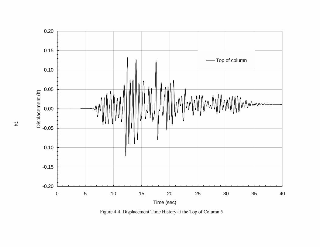
For the convenience of describing the seismic response results, the columns and bearings in bent

2 through bent 4 are re-numbered as shown in Figure 4-3. The displacement time history at the

top and bottom of column 5 in bent 3 is shown in Figures 4-4 and 4-5, respectively. The

moment, shear force, and axial force time histories at the bottom of column 5 are shown in

Figure 4-6 through Figure 4-8. Table 4-1 shows the maximum displacements at various parts of

46

the bridge. In the table, the displacements of the super structure and the cap beam are measured

at bent 3. Table 4-2 shows the maximum moment, shear force and axial force at the bottom of

the columns. From evaluations of this type of bridge, it is found that damage may occur in

bearings and columns; thus, only bearings and columns are considered in the seismic damage

assessment.

4.2 Seismic Damage Assessment of Bearings

As shown in Figure 2-3, the bridge bearing consists mainly of two one-inch diameter bolts. The

yield shear capacity byV and ultimate shear capacity buV of the bearing are determined in

Section 2.3. When the shear force acting on the bearing is less than the yield shear capacity of

the bearing, the bolts in the bearing are within the elastic limit, and the bearing sustains no

damage. When the shear force is greater than the yield shear capacity but less than the ultimate

shear capacity, the bolts are yielding. When the shear force is greater than the ultimate shear

capacity, the bolts are broken and bearing failure occurs. The criteria for the damage assessment

of the bearing are summarized in Table 4-3.

The shear forces of all the bearings resulting from the seismic response analysis of the bridge are

shown in Table 4-4. For bent 2, the shear force of bearing 6 is greater than the shear yield

strength of bearing byV (50 kips) but less than the ultimate shear strength buV (72 kips);

therefore, the bearing is in the yielding damage state. For bent 3, the shear forces of a few

bearings (bearings 15, 17-19) are greater than byV but less than buV , so these bearings are

yielding. The shear forces of all other bearings are less than the shear yield strength byV ; thus,

these bearings do not sustain any damage. The damage states of all the bearings are summarized

in Table 4-4.

47

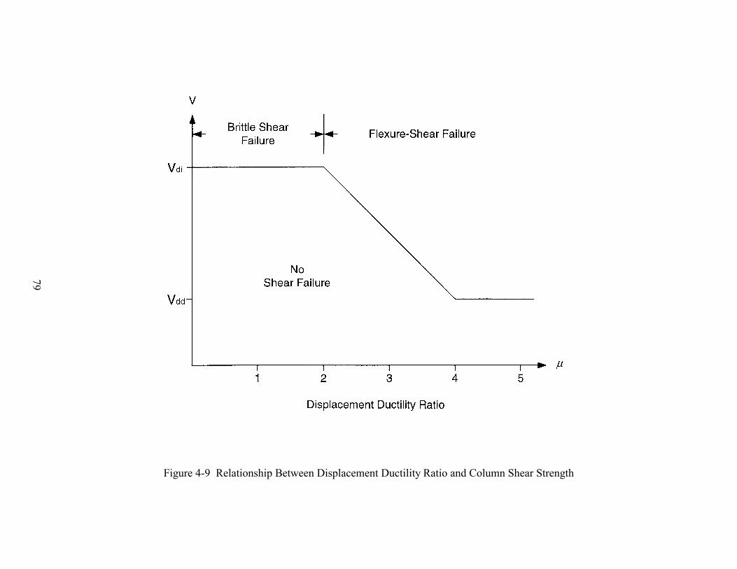
4.3 Seismic Damage Assessment of Columns in Shear

Following Seismic Retrofitting Manual for Highway Bridges (1995), the criteria for assessing

column shear failure are illustrated in Figure 4-9. In the figure, Vdi is the initial shear strength

and Vdd is the ductile shear strength.

The shear strength of columns can be expressed as (Priestley et al., 1996)

pscdddi VVV)(VV ++= (4-1)

where cV is the shear carried by concrete shear-resisting mechanism; sV is the shear carried by

transverse reinforcement shear resisting mechanisms, and pV is the shear carried by axial

compression.

The shear strength carried by concrete cV is determined as

'cgc fkA.V 80= (4-2)

where gA is the column gross cross section area and k is the concrete shear resistance factor (3.5

for initial shear strength and 1.2 for ductile shear strength).

For initial shear failure, the shear strength carried by concrete ciV is computed as

kips./kπ.Vci 19353551000450043680

2=×=×=

For ductile shear failure, the shear strength carried by concrete cdV is computed as

48

kips./kπ.Vcd 6621551000450043680

2=×=×=

The shear strength carried by transverse reinforcement is

θs

DfAπV'

yhsps cot

2= (4-3)

where D′ is the core dimension from center to center of peripheral hoop, s is the space of

peripheral hoop, Asp is the area of spiral reinforcement, and θ is the angle of cracking. In this

study, θ is taken as 30° as recommended by Priestley et al. (1996).

For the columns used in this study,

kips...πVs 134430cot12

328481102

=××××= �

The shear strength from axial compression is given by

αPVp tan= (4-4)

where α is the angle between the column axis and the line joining the centers of flexural

compression at the top and bottom of the column. The following approximation is used to

compute tanα .

c

btL

)C(C.Dα +−= 50tan (4-5)

where tC is the depth of compressive stress block at the top of column, bC is the depth of

compressive stress block at the bottom of column, P is the axial force in the column and cL is

49

the length of column. The determination of tanα for all the columns is given in Table 4-5. The

shear strength of all the columns is summarized in Table 4-6. As shown in Table 4-2, the

maximum shear force in the columns is 122 kips, which is less than the ductile shear strength

ddV of the column (147.10 kips to 155.85 kips) listed in Table 4-6; therefore, all of the columns

do not sustain any shear damage.

4.4 Seismic Damage Assessment of Columns in Flexure

From the results of the seismic response analysis, if the column moment is less than M1, the

reinforcement is in the elastic stage and the concrete may have minor cracking. Under this

condition, the column is considered as no damage. When the column moment is larger than 1M

and less than yM , the tensile reinforcement reaches yielding already and the concrete may have

visible minor cracking; thus, the column is considered in the stage of cracking. When the

column moment is larger than yM , the plastic hinge begins to form at the column. For the

column with lap splices at the bottom of the column, 2pθ is the plastic hinge rotation with cε

equal to 0.002. If the column plastic hinge rotation is larger than 2pθ , the column core starts to

disintegrate and the column is considered to fail in flexure. For the column without lap splices at

the bottom of the column, 4pθ is the plastic hinge rotation with cε equal to 0.004. If the

column plastic hinge rotation is larger than 4pθ , the column core starts to disintegrate and the

column is considered to fail in flexure. The criteria for seismic damage assessment of columns

with or without lap splices in flexure are shown in Tables 4-7 and 4-8.

As described in Section 2, the moment-curvature relation of a column section is determined

using the program BIAX. From the moment-curvature curve, the characteristic moments and

curvatures at the top and bottom of all the columns are determined and shown in Tables 4-9 and

4-10. According to Priestley et al. (1996), the plastic hinge length of column when the plastic

hinge forms against a supporting member, such as the footing, is given by

ksi)in(fdf.L.L yblyp 150080 += (4-6)

50

Where, L is the distance from the critical section of the plastic hinge to the point of

contraflexure, and bld is the diameter of the longitudinal reinforcement. In this study,

in90f5.7215 === t/L , in8750.dbl = , kips848.f y = . Therefore, the plastic hinge length is

ft.in.....Lp 11613875084815090080 ≈=××+×=

The plastic hinge rotation 2pθ is computed as follows (Seismic, 1995):

pyp )Lθ φφ −= 22 ( (4-7)

where 2pθ is the plastic hinge rotation at 002.0=cε , and 2φ is the curvature at 002.0=cε .

Table 4-11 displays the determination of 2pθ . Similarly, the determination of 4pθ is shown in

Table 4-12. From the seismic response analysis of the bridge, the maximum displacements and

maximum forces at the top and bottom of all the columns are obtained and shown in Tables 4-13

through 4-16. The damage to the top and bottom of all the columns are determined and shown in

Tables 4-17 and 4-18.

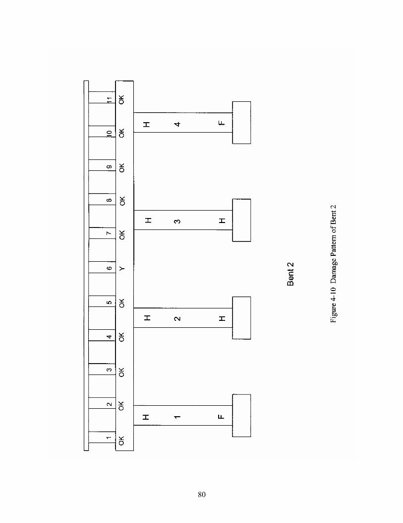
The damage patterns of bents 2 and 3 caused by the earthquake are displayed in Figures 4-10 and

4-11. It is noted that the damage pattern of bent 4 is the same as that of bent 2. As shown in the

figures, this earthquake causes damage to columns and bearings. At the bottom of the column,

all the outer columns fail in flexure, but the inner columns only form plastic hinges. At the top

of the columns, all the columns form plastic hinges without the failure in flexure. The bearings

also are yielding at several locations as shown in Figures 4-10 and 4-11. It is concluded that the

bridge sustains extensive damage by this earthquake.

4.5 Alternative Approach for Seismic Damage Assessment of Bridge

51

The component-by-component assessment of seismic damage to a bridge as described in

previous sections is appropriate when detailed seismic damage assessment is required, for

example, the assessment of a bridge for seismic retrofit. For other purposes, for example,

seismic fragility analysis, an alternative approach is desirable to assess the overall seismic

damage to a bridge. For the bridge selected for this study, the bridge columns with the lap

splices at the bottom of the columns are most vulnerable to earthquakes. When the bridge is

subject to ground motion in the transverse direction, the vibration of the bridge is dominant by

the fundamental mode in the transverse direction. As a result, the seismic responses of all

columns in all the bents are similar, and the response of column 5 of bent 3 is selected to

represent the responses of all the columns. In this study, damage to a column is determined

using the relative displacement ductility ratio of a column, which is defined as

1cy

dµ∆

∆= (4-8)

where ∆ is the relative displacement at the top of a column obtained from seismic response

analysis of the bridge, and 1cy∆ is the relative displacement of a column when the vertical

reinforcing bars at the bottom of the column reaches the first yield.

In this study, seismic damage to a bridge is classified into five damage states as defined in the

HAZUS99 (1999). These five damage states range from no damage to complete damage, and

are described in Table 4-19. Furthermore, the five damage states are quantified in terms of the

relative displacement ductility ratios as shown in Table 4-20. In the table, 1cyµ is the first yield

displacement ductility ratio, cyµ is the yield displacement ductility ratio, 2cµ is the

displacement ductility ratio with 002.0=ε c , and maxcµ is the maximum displacement ductility

ratio. It is noted that the displacement ductility ratio is defined in terms of the first yield

displacement; thus, 1cyµ is equal to 1.

Under seismic loading, column 5 is deformed in double curvature. At the first yielding, the

relative displacement at the top of the column 5 is computed as

52

1'

1 2 ∆×=∆cy (4-9)

and 1'∆ is determined as (Seismic, 1995)

3

21'

1Lφ=∆ (4-10)

Substituting 1φ = ft/110002.1 3−× (Table 4-9), and L = 7.5 ft into equation 4-10, 1'∆ is obtained

as

ftL 2232

1'1 1088.1

3)2/15(10002.1

3−

−×=××==∆ φ

and

ftcy 0376.02 1'

1 =∆×=∆

The yield displacement of the column is computed in a similar way:

ftLy

y2

232' 1025.2

3)2/15(102.1

3−

−×=××==∆

φ

and

ftycy 045.02 ' =∆×=∆

The yield displacement ductility ratio is

20.10376.0045.0

1==

∆∆

=cy

ycy

cµ

53

Given the plastic hinge length and the plastic hinge rotation of a column with 002.0=ε c , the

plastic hinge displacement 2p∆ is computed as

)2

(22p

ppL

Lθ −=∆ (4-11)

For column 5, the plastic hinge displacement 2p∆ is

ft

LLθ p

pp

2

3

22

10211.2

)21.115(1053.1

)2

(

−

−

×=

−×=

−=∆

The total displacement of the column is

22 pcyc ∆+∆=∆ (4-12)

ftpcyc 0661.0104987.2105.4 2222 =×+×=∆+∆=∆ −−

The displacement ductility ratio at 002.0=cε is

76.10376.00661.0

1

22 ==

∆

∆=

cyc

cµ

Following Seismic Retrofitting Manual for Highway Bridges (1995), the maximum displacement

ductility ratio is computed as 32max += cc µµ . The maximum ductility ratio of column 5 is

76432max .µµ cc =+=

54

From the SAP2000 analysis result, the displacements at the top and bottom of column 5 are as

follows:

fttop 1325.0=∆

ftbottom 06373.0=∆

The relative displacement between the top and bottom of the column is

ftbottomtop 06877.006373.01325.0 =−=∆−∆=∆

The displacement ductility ratio is

83.10376.0

06877.0µ1

==∆

∆=cy

d

The displacement ductility ratio of the column is

2max µµµ cdc >>

According to the criteria shown in Table 4-20, the bridge sustains extensive damage from the

earthquake.

The evaluation of bridge damage in terms of the column ductility ratio in Section 4.5 reaches the

same damage state as the bridge is evaluated using detailed component-by-component approach

as shown in the previous sections. Thus, the column ductility ratio can be used to express the

overall damage to the entire bridge.

55

Table 4-1 Maximum Displacements Resulting From Earthquake

Location Maximum displacement (ft)

Super structure 0.1345

Cap beam 0.1334

Top 0.1254 Column 1

Bottom 0.0609

Top 0.1325 Column 5

Bottom 0.0637

Abutment 0.1175

56

Table 4-2 Maximum Forces at the Bottom of Columns

Columns Axial force (kips)

Moment (kips-ft)

Shear force (kips)

1 392 -842 -115

2 302 857 117

3 302 -854 -115

4 395 843 116

5 445 -881 -120

6 358 900 122

7 357 -900 -122

8 449 883 122

57

Table 4-3 Damage Assessment Criteria for Bearings

Criteria Description of damage Bearing status

byVV < No damage to A307 Swedge bolts No Damage (OK)

buby VVV <≤ A307 Swedge bolts yielding Yielding (Y)

buVV ≥ A307 Swedge bolts broken Failure (F)

58

Table 4-4 Damage Assessment of Bearings

Bearings Shear force (kips) Bearing status

1 11.9 OK

2 13.5 OK

3 46.7 OK

4 49.7 OK

5 47.6 OK

6 51.3 Y

7 48.4 OK

8 49.0 OK

9 47.9 OK

10 13.7 OK

11 12.1 OK

12 14.1 OK

13 14.2 OK

14 48.9 OK

15 51.9 Y

16 49.9 OK

17 52.8 Y

18 50.6 Y

19 51.3 Y

20 49.5 OK

21 14.1 OK

22 14.2 OK

59

Table 4-5 Determination of tanα

Columns P (kips)

tC (in)

bC (in)

cL (in)

D (in)

αtan

1 263 10.6 10.8 180 36 0.141

2 282 10.8 11 180 36 0.139

3 282 10.8 11 180 36 0.139

4 263 10.6 10.8 180 36 0.141

5 313 11.1 11.4 180 36 0.138

6 338 11.6 11.7 180 36 0.135

7 338 11.6 11.7 180 36 0.135

8 313 11.1 11.4 180 36 0.138

60

Table 4-6 Summary of Column Shear Strength

Columns pV

(kips)

sV

(kips)

ciV (kips)

cdV (kips)

diV (kips)

ddV (kips)

1 36.97 44.13 193 66 274.10 147.10

2 39.32 44.13 193 66 276.45 149.45

3 39.32 44.13 193 66 276.45 149.45

4 36.97 44.13 193 66 274.10 147.10

5 43.04 44.13 193 66 280.17 153.17

6 45.72 44.13 193 66 282.85 155.85

7 45.72 44.13 193 66 282.85 155.85

8 43.04 44.13 193 66 280.17 153.17

61

Table 4-7 Seismic Damage Assessment Criteria for Columns with Splice in Flexure

Criteria Description of damage Column status

MM >1 No reinforcing steel yielding, minor cracking in concrete

No Damage (OK)

1MMM y ≥> Tensional reinforcement yielding and extensive cracking in concrete

Cracking (C)

2, pyMM θθ <≥ Hinging in column, but no failure of column

Hinging (H)

2, pyMM θθ >≥ Flexural failure of column Flexural failure (F)

Table 4-8 Seismic Damage Assessment Criteria for Columns without Splice in Flexure

Criteria Description of damage Column status

MM >1 No reinforcing steel yielding, minor cracking in concrete

No Damage (OK)

1MMM y ≥> Tensional reinforcement yielding and extensive cracking in concrete

Cracking (C)

4, pyMM θθ <≥ Hinging in column, but no failure of column

Hinging (H)

4, pyMM θθ >≥ Flexural failure of column Flexural failure (F)

62

Table 4-9 Characteristic Moments and Curvatures at the Top of Columns

Columns Position P (kips)

1φ (1/ft)

1M (kips-ft)

yφ (1/ft)

yM (kips-ft)

1 Top 249 1.07E-03 705 1.26E-03 830

2 Top 267 1.05E-03 714 1.24E-03 844

3 Top 267 1.05E-03 714 1.24E-03 844

4 Top 249 1.07E-03 705 1.26E-03 830

5 Top 298 1.02E-03 728 1.21E-03 869

6 Top 323 9.92E-04 738 1.20E-03 888

7 Top 323 9.92E-04 738 1.20E-03 888

8 Top 298 1.02E-03 728 1.21E-03 869

Table 4-10 Characteristic Moments and Curvatures at the Bottom of Columns

Columns Position P (kips)

1φ (1/ft)

1M (kips-ft)

yφ (1/ft)

yM (kips-ft)

1 Bottom 263 1.06E-03 712 1.25E-03 841

2 Bottom 282 1.03E-03 722 1.22E-03 856

3 Bottom 282 1.03E-03 722 1.22E-03 856

4 Bottom 263 1.06E-03 712 1.25E-03 841

5 Bottom 313 1.00E-03 734 1.20E-03 881

6 Bottom 338 9.77E-04 743 1.19E-03 899

7 Bottom 338 9.77E-04 743 1.19E-03 899

8 Bottom 313 1.00E-03 734 1.20E-03 881

63

Table 4-11 Determination of 2pθ

Columns Position 2φ

(1/ft) yφ

(1/ft) yφφ −2

(1/ft) pL

(ft) 2pθ

(rad)

1 Bottom 2.73E-03 1.25E-03 1.48E-03 1.1 1.63E-03

2 Bottom 2.67E-03 1.22E-03 1.45E-03 1.1 1.59E-03

3 Bottom 2.67E-03 1.22E-03 1.45E-03 1.1 1.59E-03

4 Bottom 2.73E-03 1.25E-03 1.48E-03 1.1 1.63E-03

5 Bottom 2.59E-03 1.20E-03 1.39E-03 1.1 1.53E-03

6 Bottom 2.52E-03 1.19E-03 1.33E-03 1.1 1.46E-03

7 Bottom 2.52E-03 1.19E-03 1.33E-03 1.1 1.46E-03

8 Bottom 2.59E-03 1.20E-03 1.39E-03 1.1 1.53E-03

64

Table 4-12 Determination of 4pθ

Columns Position 4φ

(1/ft) yφ

(1/ft) yφφ −4

(1/ft) pL

(ft) 4pθ

(rad)

1 Top 5.84E-03 1.26E-03 4.58E-03 1.1 5.04E-03

2 Top 5.72E-03 1.24E-03 4.49E-03 1.1 4.94E-03

3 Top 5.72E-03 1.24E-03 4.49E-03 1.1 4.94E-03

4 Top 5.84E-03 1.26E-03 4.58E-03 1.1 5.04E-03

5 Top 5.56E-03 1.21E-03 4.34E-03 1.1 4.78E-03

6 Top 5.45E-03 1.20E-03 4.25E-03 1.1 4.67E-03

7 Top 5.45E-03 1.20E-03 4.25E-03 1.1 4.67E-03

8 Top 5.56E-03 1.21E-03 4.34E-03 1.1 4.78E-03

65

Table 4-13 Maximum Displacements at the Top of Columns

Column Position Vertical displacement (ft)

Horizontal displacement (ft)

θ (rad)

1 Top -1.06E-04 -1.66E-05 1.62E-03

2 Top -7.01E-05 -1.70E-05 1.81E-03

3 Top -8.10E-05 -1.70E-05 1.80E-03

4 Top -3.45E-05 -1.66E-05 1.60E-03

5 Top -1.21E-04 -1.75E-05 1.82E-03

6 Top -8.58E-05 -1.79E-05 1.95E-03

7 Top -9.68E-05 -1.79E-05 1.94E-03

8 Top -4.78E-05 -1.75E-05 1.79E-03

Table 4-14 Maximum Forces at the Top of Columns

Column Position Axial force (kips)

Shear force (kips)

Moment (kip-ft)

1 Top -123.19 108.19 -828.50

2 Top -287.28 110.61 -842.83

3 Top -247.48 110.61 -842.83

4 Top -374.68 108.19 -828.50

5 Top -170.03 113.32 -867.33

6 Top -342.92 116.47 -889.06

7 Top -303.49 116.47 -889.06

8 Top -425.98 113.32 -867.32

66

Table 4-15 Maximum Displacements at the Bottom of Columns

Column Position Vertical displacement (ft)

Horizontal displacement (ft)

θ (rad)

1 Bottom -3.74E-05 1.80E-05 1.74E-03

2 Bottom -8.49E-05 1.85E-05 1.18E-03

3 Bottom -7.45E-05 1.85E-05 1.18E-03

4 Bottom -1.12E-04 1.80E-05 1.74E-03

5 Bottom -5.03E-05 1.88E-05 1.89E-03

6 Bottom -1.01E-04 1.95E-05 1.27E-03

7 Bottom -9.01E-05 1.95E-05 1.27E-03

8 Bottom -1.26E-04 1.88E-05 1.89E-03

Table 4-16 Maximum Forces at the Bottom of Columns

Column Position Axial force (kips)

Shear force (kips)

Moment (kip-ft)

1 Bottom -132.25 116.96 843.33

2 Bottom -300.59 120.31 859.01

3 Bottom -263.64 120.31 859.01

4 Bottom -395.10 116.97 843.33

5 Bottom -178.10 122.45 883.35

6 Bottom -357.15 126.76 902.64

7 Bottom -318.73 126.75 902.64

8 Bottom -447.38 122.45 883.35

67

Table 4-17 Determination of Damage Status at the Top of Columns

Demand Capacity Column Position

Moment (kip-ft) θ 1M yM 4pθ Column status

1 Top 828.50 1.62E-03 705 830 5.04E-03 H

2 Top 842.83 1.81E-03 714 844 4.94E-03 H

3 Top 842.83 1.80E-03 714 844 4.94E-03 H

4 Top 828.50 1.60E-03 705 830 5.04E-03 H

5 Top 867.33 1.82E-03 728 869 4.78E-03 H

6 Top 889.06 1.95E-03 738 888 4.67E-03 H

7 Top 889.06 1.94E-03 738 888 4.67E-03 H

8 Top 867.32 1.79E-03 728 869 4.78E-03 H

68

Table 4-18 Determination of Damage Status at the Bottom of Columns

Demand Capacity Column Position Moment

(kip-ft) θ 1M yM 2pθ

Column status

1 Bottom 843.33 1.74E-03 712 841 1.63E-03 F

2 Bottom 859.01 1.18E-03 722 856 1.59E-03 H

3 Bottom 859.01 1.18E-03 722 856 1.59E-03 H

4 Bottom 843.33 1.74E-03 712 841 1.63E-03 F

5 Bottom 883.35 1.89E-03 734 881 1.53E-03 F

6 Bottom 902.64 1.27E-03 743 899 1.46E-03 H

7 Bottom 902.64 1.27E-03 743 899 1.46E-03 H

8 Bottom 883.35 1.89E-03 734 881 1.53E-03 F

69

Table 4-19 Bridge Damage States (HAZUS99)

Damage states

Description

N No damage No damage to the structure.

S Sight/Minor damage

Minor cracking and spalling to the abutment, cracks in shear keys at abutments, minor spalling and cracks at hinges, minor spalling at the column (damage requires no more than cosmetic repair) or minor cracking to the deck.

M Moderate damage

Any column experiencing moderate (shear cracks) cracking and spalling (column structurally still sound), moderate movement of the abutment (<2�), extensive cracking and spalling of shear keys, any connection having cracked shear keys or bent bolts, keeper bar failure without unseating, rocker bearing failure or moderate settlement of the approach.

E Extensive damage

Any column degrading without collapse � shear failure � (column structurally unsafe), significant residual movement at connections, or major settlement approach, vertical offset of the abutment, differential settlement at connections, shear key failure at abutments.

C Complete damage

Any column collapsing and connection losing all bearing support, which may lead to imminent deck collapse, tilting of substructure due to foundation failure.

70

Table 4-20 Bridge Damage States Measured by Displacement Ductility Ratios

Damage states Criteria

N No damage dcy µµ >1

S Slight/Minor damage 1cydcy µµµ >>

M Moderate damage cydc µµµ >>2

E Extensive damage 2max cdc µµµ >>

C Complete damage maxcd µµ >

71

Figure 4-1 Fundamental Mode of the Bridge in the Transverse Direction

72

Figure 4-2 Fundamental Mode of the Bridge in the Longitudinal Direction

73

74

Figure 4-4 Displacement Time History at the Top of Column 5

-0.20

-0.15

-0.10

-0.05

0.00

0.05

0.10

0.15

0.20

0 5 10 15 20 25 30 35 40

Time (sec)

Dis

plac

emen

t (ft)

Top of column

75

Figure 4-5 Displacement Time History at the Bottom of Column 5

-0.20

-0.15

-0.10

-0.05

0.00

0.05

0.10

0.15

0.20

0 5 10 15 20 25 30 35 40

Time (sec)

Dis

plac

emen

t (ft)

Bottom of column

76

Figure 4-6 Moment Time History at the Bottom of Colume 5

-1000

-800

-600

-400

-200

0

200

400

600

800

1000

0 5 10 15 20 25 30 35 40

Time (sec)

Mom

ent (

kips

-ft)

77

Figure 4-7 Shear Force Time History at the Bottom of Colume 5

-200

-150

-100

-50

0

50

100

150

200

0 5 10 15 20 25 30 35 40

Time (sec)

Shea

r For

ce (k

ips)

78

Figure 4-8 Axial Force Time History at the Bottom of Colume 5

-600

-500

-400

-300

-200

-100

0

0 5 10 15 20 25 30 35 40

Time (sec)

Axia

l For

ce (k

ips)

79

Figure 4-9 Relationship Between Displacement Ductility Ratio and Column Shear Strength

80

81

82

SECTION 5

UNCERTAINTIES IN THE EARTHQUAKE-SITE-BRIDGE SYSTEM

The uncertainties in parameters used in modeling earthquake, site condition, and bridge are

considered in this section.

5.1 Uncertainty in Earthquake Modeling

In the generation of earthquake ground motion at the rock outcrop, uncertainties in earthquake

source, seismic wave propagation, and rock condition near the ground surface are considered.

The seismic parameters, such as the stress parameter ∆σ, quality factor Q, and the attenuation

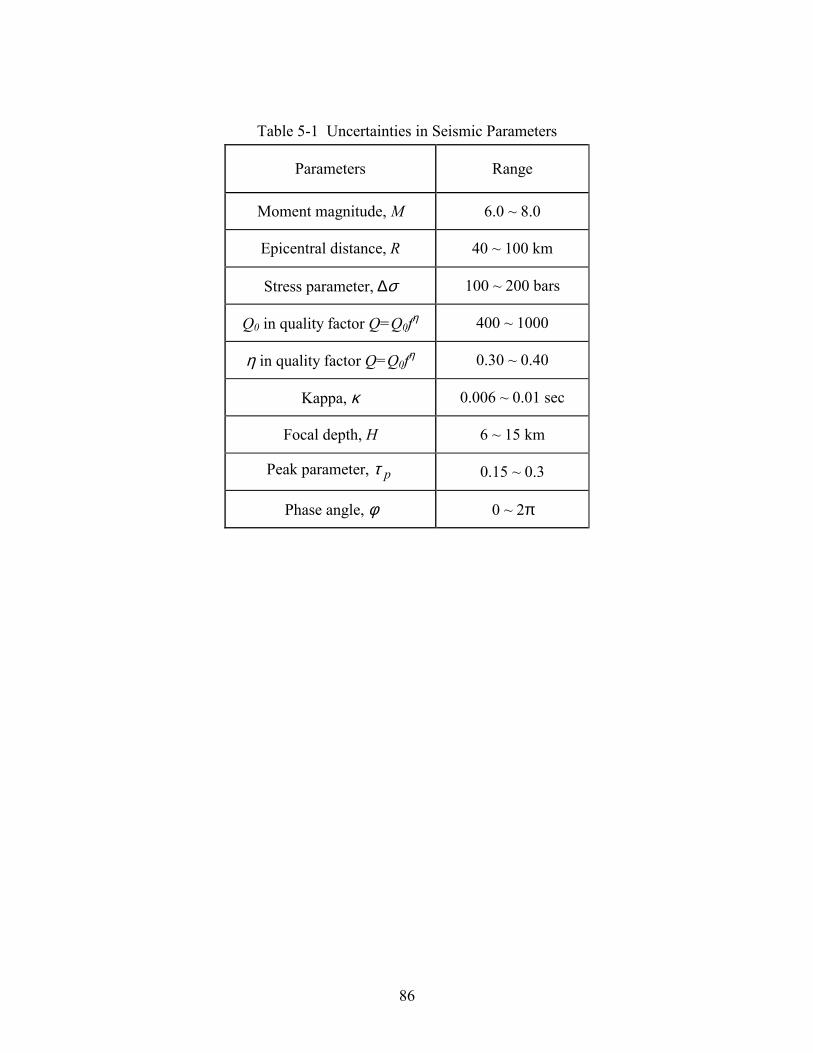
parameter κ have significant effects on the resulting ground motion. From a literature review

(Guidelines, 1993; Hwang and Huo, 1994), the random seismic parameters are identified and

shown in Table 5-1. These parameters are considered to follow a uniform distribution. In Table

5-1, the parameter φ is the random phase angle, which is used to generate a time series of random

band-limited white Gaussian noise. The time at which the peak of the acceleration occurs is also

considered as a random variable. It is noted that the strong motion duration eT is determined

from the stress parameter and other seismic parameters; thus, the duration of ground motion will

vary as different values are assigned to these seismic parameters.

For each random seismic parameter listed in Table 5-1, 100 samples are generated according to

its distribution function. The exceptions are the two parameters defining the quality factors. For

these two parameters, only 10 samples are established as shown in Table 5-2. These samples are

then combined using the Latin Hypercube sampling technique to establish 100 sets of seismic

parameters as shown in Table 5-3. For each set of seismic parameters, an acceleration time

history at the rock outcrop is generated using the method described in Section 3. Thus, a total of

100 acceleration time histories at the rock outcrop are generated for this study.

5.2 Uncertainties in Soil Modeling

In this study, the computer program SHAKE91 is used to perform the nonlinear site response

83

analysis. The input soil parameters include the low strain shear modulus, shear modulus

reduction curves and damping ratio curves. The uncertainties in these soil parameters

established by Hwang and Huo (1994) are utilized in this study.

The low strain shear modulus of soils is estimated using empirical formulas. For sandy soils, the

low strain shear modulus is a function of the relative density rD (Equation 3-13) and for clayey

soils, the low strain shear modulus is a function of the undrained shear strength uS (Equation 3-

14). The ranges of these two soil parameters are listed in Table 5-4, and these two soil

parameters are assumed to follow a uniform distribution.

Figure 5-1 shows the shear modulus reduction curves and damping ratio curves for sandy soils.

For clayey soils, the shear modulus reduction curves and damping ratio curves are a function of

the plasticity index PI. The shear modulus reduction curves and damping ratio curves for clays

with PI = 15 and 50 are shown in Figures 5-2 and 5-3, respectively. An upper bound curve and a

lower bound curve are also shown in Figures 5-1 through 5-3. The upper bound curve

corresponds to the mean value plus two standard deviations, while the lower bound curve

corresponds to the mean value minus two standard deviations (Hwang and Huo, 1994).

The random soil parameters are the relative density of sand rD , undrained shear strength of clay

uS , shear modulus reduction curves, and the corresponding damping ratio curves. For each soil

parameter, 10 samples are generated. For example, Figures 5-4 and 5-5 show 10 samples of

shear modulus reduction curves and corresponding damping ratio curves for clays with PI = 15.

These samples of soil parameters are used to construct 10 samples of the soil profile, which are

denoted as soil profile 1 to soil profile 10. Each sample of soil profile is matched with 10

samples of acceleration time history at the rock outcrop to establish 100 earthquake-site samples.

For each earthquake-site sample, an acceleration time history at the ground surface is generated

from a nonlinear site response analysis using SHAKE91.

84

5.3 Uncertainty in Bridge Modeling

The bridge model includes the bridge itself and supporting springs representing pile footings and

abutments. The uncertainty in modeling the bridge itself is mainly due to the uncertainties

associated with construction materials, namely, concrete and reinforcement. This uncertainty

affects the strength and stiffness of structural members and the nonlinear behavior of columns.

The uncertainties in supporting springs are mainly from surrounding soils. This uncertainty

affects the stiffness of supporting springs.

Following Hwang and Huo (1998), the concrete compressive strength with design value of 3.0

ksi is assumed to have a normal distribution with a mean strength of 4.5 ksi and a coefficient of

variation (COV) of 0.2. The yield strength of grade 40 reinforcement is described by a

lognormal distribution with a mean value of 48.8 ksi and a COV of 0.11. Ten samples of

concrete compressive strength and steel yield strength are generated with each sample in the one-

tenth of the probability distributions. These samples are combined using the Latin Hypercube

sampling technique to create 10 bridge samples, numbered from bridge sample 1 to bridge

sample 10 as shown in Table 5-5. For all bridge samples, the moment-curvature relations of

column sections are derived using BIAX. Based on these moment-curvature relationships, the

nonlinear characteristics of column sections are determined and used in the nonlinear seismic

response analyses of bridges. Thus, uncertainties in nonlinear behavior of columns are included

in the seismic response analysis and seismic damage assessment of bridges.

The uncertainty in modeling spring stiffness of pile footings and abutments is taken into account

in this study. Spring stiffness is considered to follow a uniform distribution. The mean values

are determined as described in Section 2. The coefficient of variation is taken as 30%, since the

uncertainties of random soil parameters listed in Table 5-4 are in the range of 20%~33%. Ten

samples of spring stiffness are generated according to the distribution and are listed in Tables 5-6

(pile footings) and 5-7 (abutments). Each sample of spring stiffness is assigned to a bridge

sample.

85

5.4 Generation of Earthquake-Site-Bridge Samples

In this study, each bridge sample is matched with a soil profile sample, and 10 earthquake

samples as illustrated in Figure 5-6. Therefore, a total of 100 earthquake-site-bridge samples as

listed in Table 5-8 are established for the seismic response analysis.

86

Table 5-1 Uncertainties in Seismic Parameters

Parameters Range

Moment magnitude, M 6.0 ~ 8.0

Epicentral distance, R 40 ~ 100 km

Stress parameter, ∆σ 100 ~ 200 bars

Q0 in quality factor Q=Q0fη 400 ~ 1000

η in quality factor Q=Q0fη 0.30 ~ 0.40

Kappa, κ 0.006 ~ 0.01 sec

Focal depth, H 6 ~ 15 km

Peak parameter, pτ 0.15 ~ 0.3

Phase angle, φ 0 ~ 2π

87

Table 5-2 Ten Samples of Quality Factor Parameters

Sample Q0 η

1 1000 0.30

2 930 0.31

3 870 0.32

4 800 0.33

5 730 0.34

6 680 0.36

7 600 0.37

8 530 0.38

9 470 0.39

10 400 0.4

88

Table 5-3 Summary of Seismic Parameters Earthquake

number M R (km)

∆σ (bars) Qo η H

(km) κ

(sec) τp

1 6.3 50 161 1000 0.30 6.6 0.0077 0.272 6.7 89 153 930 0.31 7.8 0.0088 0.173 7.7 84 124 870 0.32 6.6 0.0068 0.244 6.7 65 160 800 0.33 14.8 0.0068 0.175 7.3 55 103 730 0.34 14.8 0.0081 0.256 6.4 85 154 680 0.36 8.1 0.0061 0.287 6.2 45 103 600 0.37 12.2 0.0062 0.278 6.5 89 109 530 0.38 9.0 0.0087 0.199 6.7 81 116 470 0.39 13.7 0.0095 0.16

10 6.3 95 153 400 0.40 10.7 0.0099 0.2011 6.4 95 198 1000 0.30 9.3 0.0098 0.2412 7.3 75 145 930 0.31 6.1 0.0079 0.1913 6.5 100 113 870 0.32 9.6 0.0071 0.1714 6.1 91 144 800 0.33 11.0 0.0082 0.1815 6.0 56 116 730 0.34 8.6 0.0070 0.3016 7.8 99 169 680 0.36 13.2 0.0071 0.2417 7.5 43 172 600 0.37 10.1 0.0095 0.2718 6.1 48 163 530 0.38 11.4 0.0078 0.1519 7.3 63 147 470 0.39 12.4 0.0098 0.2820 6.5 66 130 400 0.40 12.6 0.0061 0.2921 6.7 65 106 1000 0.30 11.6 0.0067 0.2122 7.4 73 178 930 0.31 10.9 0.0069 0.2623 6.4 50 158 870 0.32 11.0 0.0067 0.2624 7.0 48 170 800 0.33 7.1 0.0088 0.2625 7.9 94 153 730 0.34 7.8 0.0099 0.2226 6.1 81 198 680 0.36 12.2 0.0091 0.1627 6.8 96 102 600 0.37 11.5 0.0061 0.2128 7.6 97 143 530 0.38 14.3 0.0076 0.2429 7.9 94 131 470 0.39 14.2 0.0070 0.2630 7.2 55 120 400 0.40 10.8 0.0092 0.3031 7.7 72 127 1000 0.30 13.2 0.0075 0.2032 7.3 54 165 930 0.31 8.6 0.0061 0.2533 8.0 99 143 870 0.32 13.1 0.0079 0.2334 6.9 94 197 800 0.33 8.7 0.0067 0.2735 6.6 90 183 730 0.34 13.1 0.0093 0.2936 6.7 78 141 680 0.36 6.4 0.0084 0.2837 7.0 90 180 600 0.37 13.7 0.0094 0.2238 6.5 42 183 530 0.38 13.1 0.0067 0.2539 7.6 98 199 470 0.39 8.6 0.0072 0.2540 7.5 89 122 400 0.40 12.7 0.0084 0.2141 7.2 70 136 1000 0.30 12.6 0.0097 0.1642 7.2 92 179 930 0.31 8.2 0.0091 0.2343 7.8 95 151 870 0.32 12.2 0.0089 0.1944 8.0 48 164 800 0.33 14.8 0.0089 0.2545 7.4 46 150 730 0.34 10.8 0.0093 0.2546 7.2 55 109 680 0.36 7.7 0.0074 0.2347 6.3 82 146 600 0.37 13.1 0.0076 0.2948 7.9 61 176 530 0.38 9.7 0.0093 0.2149 6.1 64 132 470 0.39 7.2 0.0074 0.1650 7.3 48 186 400 0.40 7.1 0.0074 0.28

89

Table 5-3 Summary of Seismic Parameters (Continued) Earthquake

number M R (km)

∆σ (bars) Qo η H

(km) κ

(sec) τp

51 6.3 79 170 1000 0.30 9.0 0.0081 0.2352 7.6 64 120 930 0.31 9.4 0.0066 0.2453 6.6 64 195 870 0.32 9.9 0.0093 0.1854 6.8 92 146 800 0.33 13.0 0.0078 0.1955 7.5 45 160 730 0.34 7.4 0.0091 0.1856 7.6 41 157 680 0.36 7.9 0.0079 0.1557 6.9 75 153 600 0.37 14.8 0.0080 0.2958 6.2 90 135 530 0.38 9.7 0.0090 0.2159 7.4 78 191 470 0.39 9.6 0.0090 0.2760 7.2 74 196 400 0.40 12.8 0.0066 0.2161 6.6 88 197 1000 0.30 9.5 0.0068 0.2862 6.6 54 153 930 0.31 12.8 0.0069 0.2763 7.8 79 134 870 0.32 11.4 0.0091 0.1764 7.4 72 107 800 0.33 8.0 0.0092 0.1865 6.4 66 125 730 0.34 13.6 0.0092 0.2066 6.7 49 174 680 0.36 7.3 0.0083 0.2967 6.4 41 129 600 0.37 8.3 0.0085 0.2868 6.3 85 131 530 0.38 7.1 0.0097 0.2569 6.2 45 167 470 0.39 14.0 0.0097 0.1870 7.8 75 142 400 0.40 8.2 0.0072 0.2571 7.3 83 197 1000 0.30 8.9 0.0095 0.1972 7.9 43 124 930 0.31 9.0 0.0083 0.2373 6.8 66 116 870 0.32 12.1 0.0095 0.2674 7.0 99 200 800 0.33 9.5 0.0070 0.1975 6.1 59 172 730 0.34 13.1 0.0084 0.2376 7.8 62 126 680 0.36 13.1 0.0090 0.2177 7.3 52 157 600 0.37 14.9 0.0063 0.3078 7.5 65 127 530 0.38 11.3 0.0076 0.2179 6.5 86 164 470 0.39 6.5 0.0061 0.2080 7.4 75 136 400 0.40 14.4 0.0093 0.1981 6.0 97 174 1000 0.30 12.6 0.0079 0.2982 6.0 89 178 930 0.31 7.8 0.0071 0.1583 7.2 86 108 870 0.32 7.1 0.0097 0.1984 6.9 41 112 800 0.33 12.7 0.0095 0.2685 6.3 66 191 730 0.34 6.1 0.0084 0.2086 6.4 79 164 680 0.36 6.7 0.0070 0.2187 7.6 52 120 600 0.37 10.9 0.0061 0.1888 7.0 65 163 530 0.38 10.8 0.0095 0.2189 7.6 82 188 470 0.39 13.2 0.0078 0.2090 6.9 55 113 400 0.40 12.9 0.0092 0.2091 6.0 65 106 1000 0.30 13.8 0.0089 0.2192 7.4 98 194 930 0.31 11.4 0.0061 0.2793 6.5 60 169 870 0.32 9.9 0.0061 0.2594 6.8 51 108 800 0.33 13.2 0.0071 0.1995 8.0 69 163 730 0.34 12.0 0.0095 0.3096 7.7 84 157 680 0.36 11.4 0.0084 0.2197 7.1 45 166 600 0.37 7.9 0.0064 0.2898 7.0 73 162 530 0.38 9.9 0.0095 0.2699 7.1 59 110 470 0.39 11.0 0.0096 0.26100 7.4 93 138 400 0.40 12.2 0.0090 0.22

90

Table 5-4 Uncertainty in Soil Parameters

Soil classification Random variable Range

Very loose 0.00~0.15

Loose 0.15~0.35

Medium dense 0.35~0.65

Dense 0.65~0.85

Sand

Very dense

rD

0.85~1.00

Very soft 0.00~11.98 (kN/m2)

Soft 11.98~23.95 (kN/m2)

Medium stiff 23.95~47.90 (kN/m2)

Stiff 47.90~95.80 (kN/m2)

Very stiff 95.80~191.60 (kN/m2)

Clay

Hard

uS

191.60~383.20 (kN/m2)

91

Table 5-5 Material Values of Ten Bridge Samples

Concrete strength and elastic module Reinforcing steel strength Bridge sample

cf ( ksi ) cf ( ksf ) E ( ksf ) yf ( ksi ) yf ( ksf )

1 3.89 560.6 512126 40.49 5830.6

2 3.57 513.7 490232 43.29 6234.2

3 4.39 631.7 543646 49.20 7084.3

4 3.02 434.8 451039 46.51 6697.1

5 4.85 697.9 571432 52.26 7525.2

6 5.11 735.4 586573 45.05 6487.4

7 4.61 664.3 557485 58.14 8372.8

8 5.43 782.3 604991 47.86 6891.1

9 5.98 861.2 634748 50.62 7289.6

10 4.15 598.1 528968 54.38 7830.8

92

Table 5-6 Stiffness of Pile Footings

Bridge sample Lateral stiffness ( kips/ft )

Torsion stiffness ( kips/rad )

1 1344 4462

2 1472 4887

3 1600 5312

4 1728 5737

5 1856 6162

6 1984 6586

7 2112 7011

8 2240 7436

9 2368 7861

10 2496 8286

93

Table 5-7 Spring Stiffness of Abutments

Longitudinal (kips/ft) Transverse (kips/ft)Bridge sample Total spring Sub-spring Total spring Sub-spring

1 12628 1148 3278 298

2 13827 1257 3586 326

3 15037 1367 3894 354

4 16236 1476 4213 383

5 17435 1585 4521 411

6 18645 1695 4829 439

7 19844 1804 5148 468

8 21043 1913 5456 496

9 22253 2023 5764 524

10 23452 2132 6083 553

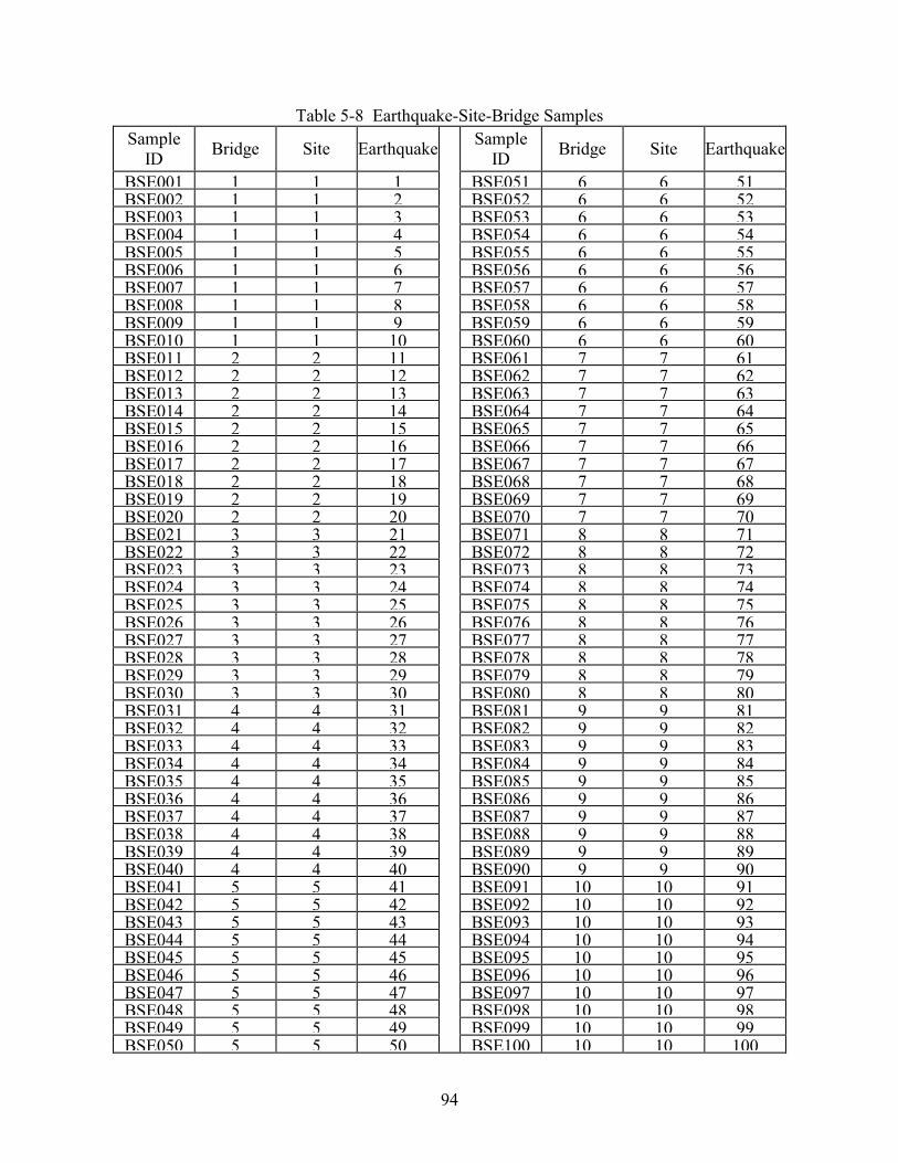
94

Table 5-8 Earthquake-Site-Bridge Samples Sample

ID Bridge Site Earthquake Sample ID Bridge Site Earthquake

BSE001 1 1 1 BSE051 6 6 51BSE002 1 1 2 BSE052 6 6 52BSE003 1 1 3 BSE053 6 6 53BSE004 1 1 4 BSE054 6 6 54BSE005 1 1 5 BSE055 6 6 55BSE006 1 1 6 BSE056 6 6 56BSE007 1 1 7 BSE057 6 6 57BSE008 1 1 8 BSE058 6 6 58BSE009 1 1 9 BSE059 6 6 59BSE010 1 1 10 BSE060 6 6 60BSE011 2 2 11 BSE061 7 7 61BSE012 2 2 12 BSE062 7 7 62BSE013 2 2 13 BSE063 7 7 63BSE014 2 2 14 BSE064 7 7 64BSE015 2 2 15 BSE065 7 7 65BSE016 2 2 16 BSE066 7 7 66BSE017 2 2 17 BSE067 7 7 67BSE018 2 2 18 BSE068 7 7 68BSE019 2 2 19 BSE069 7 7 69BSE020 2 2 20 BSE070 7 7 70BSE021 3 3 21 BSE071 8 8 71BSE022 3 3 22 BSE072 8 8 72BSE023 3 3 23 BSE073 8 8 73BSE024 3 3 24 BSE074 8 8 74BSE025 3 3 25 BSE075 8 8 75BSE026 3 3 26 BSE076 8 8 76BSE027 3 3 27 BSE077 8 8 77BSE028 3 3 28 BSE078 8 8 78BSE029 3 3 29 BSE079 8 8 79BSE030 3 3 30 BSE080 8 8 80BSE031 4 4 31 BSE081 9 9 81BSE032 4 4 32 BSE082 9 9 82BSE033 4 4 33 BSE083 9 9 83BSE034 4 4 34 BSE084 9 9 84BSE035 4 4 35 BSE085 9 9 85BSE036 4 4 36 BSE086 9 9 86BSE037 4 4 37 BSE087 9 9 87BSE038 4 4 38 BSE088 9 9 88BSE039 4 4 39 BSE089 9 9 89BSE040 4 4 40 BSE090 9 9 90BSE041 5 5 41 BSE091 10 10 91BSE042 5 5 42 BSE092 10 10 92BSE043 5 5 43 BSE093 10 10 93BSE044 5 5 44 BSE094 10 10 94BSE045 5 5 45 BSE095 10 10 95BSE046 5 5 46 BSE096 10 10 96BSE047 5 5 47 BSE097 10 10 97BSE048 5 5 48 BSE098 10 10 98BSE049 5 5 49 BSE099 10 10 99BSE050 5 5 50

BSE100 10 10 100

95

Figure 5-1 Shear Modulus Reduction and Damping Ratio Curves for Sand

0

0.2

0.4

0.6

0.8

1

0.001 0.01 0.1 1 10 100

Shear Strain Ratio

Shea

r Mod

ulus

Rat

io G

/Gm

ax

LowerUpperMean

0

5

10

15

20

25

0.0001 0.001 0.01 0.1 1

Shear Strain (%)

Dam

ping

Rat

io (%

)

Lower

Upper

Mean

96

Figure 5-2 Shear Modulus Reduction and Damping Ratio Curves for Clays with PI = 15

0

0.2

0.4

0.6

0.8

1

0.0001 0.001 0.01 0.1 1

Shear Strain (%)

Shea

r Mod

ulus

Rat

io G

/Gm

ax

LowerUpperMean

0

5

10

15

20

25

0.0001 0.001 0.01 0.1 1

Shear Strain (%)

Dam

ping

Rat

io (%

)

Lower

Upper

Mean

97

Figure 5-3 Shear Modulus Reduction and Damping Ratio Curves for Clays with PI = 50

0

0.2

0.4

0.6

0.8

1

0.0001 0.001 0.01 0.1 1

Shear Strain (%)

Shea

r Mod

ulus

Rat

io G

/Gm

ax

LowerUpperMean

0

5

10

15

20

25

0.0001 0.001 0.01 0.1 1

Shear Strain (%)

Dam

ping

Rat

io (%

)

Lower

Upper

Mean

98

99

100

101

SECTION 6

PROBABILISTIC SEISMIC DEMAND

For each earthquake-site-bridge sample list in Table 5-8, a nonlinear time history analysis is

carried out using the program SAP2000. The displacement ductility ratios of column 5 are

computed as shown in Table 6-1. It is noted that SA and PGA of each input ground motion are

also listed in the table.

The probabilistic characteristics of structural demand are described by a lognormal distribution.

dµ = Ln( )β,µ dd~ (6-1)

where dµ~ is the median value of the structural demand and βd is the logarithmic standard

deviation, which are determined from the regression analysis of the simulated response data.

The expression used in the regression analysis is

Ln(y) = a + b Ln(x) + ε (6-2)

where y is the displacement ductility ratio, x is SA or PGA, a and b are the unknown regression

coefficients, and ε is a normal random variable with a zero mean and the standard deviation σ

to represent the variation of the response data.

From the regression analysis of the response data with respect to SA, the median value of the

structural demand is determined as

Ln( dµ~ ) = 0.99 + 1.110 Ln(SA) (6-3)

The standard deviation σ is determined as 0.103. This indicates the regression line fits very

well with the response data as shown in Figure 6-1.

102

From the regression analysis of the response data versus PGA, the median value of the structural

demand is determined as

Ln( dµ~ ) = 2.115 + 1.326 Ln(PGA) (6-4)

The standard deviation σ is 0.309. This indicates that the displacement ductility ratios are

scattered when they are plotted versus PGA as shown in Figure 6-2.

103

Table 6-1 Summary of Structural Response to Earthquakes Displacements

(ft) Relative disp.

(ft) Sample ID

PGA (g)

SA (g)

sT (sec) Top Bottom Top-Bottom

Displacement ductility ratio

dµ BSE001 0.15 0.35 0.55 0.0884 0.0564 0.0320 0.85 BSE002 0.16 0.41 0.55 0.1031 0.0657 0.0374 1.00 BSE003 0.20 0.45 0.55 0.1146 0.0727 0.0419 1.12 BSE004 0.13 0.27 0.55 0.0680 0.0436 0.0244 0.65 BSE005 0.18 0.51 0.55 0.1303 0.0788 0.0515 1.37 BSE006 0.12 0.17 0.55 0.0441 0.0281 0.0160 0.43 BSE007 0.11 0.27 0.55 0.0680 0.0434 0.0246 0.65 BSE008 0.08 0.17 0.55 0.0428 0.0274 0.0154 0.41 BSE009 0.10 0.14 0.55 0.0351 0.0224 0.0127 0.34 BSE010 0.07 0.13 0.55 0.0330 0.0210 0.0120 0.32 BSE011 0.16 0.18 0.53 0.0432 0.0266 0.0166 0.44 BSE012 0.20 0.38 0.53 0.0886 0.0548 0.0338 0.90 BSE013 0.10 0.21 0.53 0.0487 0.0300 0.0187 0.50 BSE014 0.09 0.18 0.53 0.0429 0.0264 0.0165 0.44 BSE015 0.09 0.15 0.53 0.0363 0.0225 0.0138 0.37 BSE016 0.28 0.68 0.53 0.1710 0.0759 0.0951 2.53 BSE017 0.33 0.91 0.53 0.2046 0.0782 0.1264 3.36 BSE018 0.15 0.24 0.53 0.0579 0.0357 0.0222 0.59 BSE019 0.19 0.39 0.53 0.0915 0.0565 0.0350 0.93 BSE020 0.10 0.16 0.53 0.0378 0.0232 0.0146 0.39 BSE021 0.16 0.23 0.51 0.0517 0.0315 0.0202 0.54 BSE022 0.23 0.73 0.51 0.1463 0.0776 0.0687 1.83 BSE023 0.18 0.41 0.51 0.0893 0.0543 0.0350 0.93 BSE024 0.25 0.71 0.51 0.1599 0.0777 0.0822 2.19 BSE025 0.29 0.78 0.51 0.1554 0.0775 0.0779 2.07 BSE026 0.09 0.23 0.51 0.0509 0.0310 0.0199 0.53 BSE027 0.10 0.19 0.51 0.0409 0.0249 0.0160 0.43 BSE028 0.18 0.48 0.51 0.1053 0.0639 0.0414 1.10 BSE029 0.28 0.73 0.51 0.1631 0.0769 0.0862 2.29 BSE030 0.22 0.40 0.51 0.0875 0.0533 0.0342 0.91 BSE031 0.24 0.48 0.51 0.1034 0.0583 0.0451 1.20 BSE032 0.32 0.65 0.51 0.1311 0.0641 0.0670 1.78 BSE033 0.28 0.89 0.51 0.1605 0.0664 0.0941 2.50 BSE034 0.23 0.26 0.51 0.0558 0.0320 0.0238 0.63 BSE035 0.14 0.29 0.51 0.0617 0.0352 0.0265 0.71 BSE036 0.12 0.29 0.51 0.0621 0.0354 0.0267 0.71 BSE037 0.17 0.35 0.51 0.0747 0.0426 0.0321 0.85 BSE038 0.25 0.37 0.51 0.0782 0.0446 0.0336 0.89 BSE039 0.28 0.45 0.51 0.0946 0.0540 0.0406 1.08

104

Table 6-1 Summary of Structural Response to Earthquakes (Continued) Displacements

(ft) Relative disp.

(ft) Sample ID

PGA (g)

SA (g)

sT (sec) Top Bottom Top-Bottom

Displacement ductility ratio

dµ BSE040 0.17 0.35 0.51 0.0735 0.0421 0.0314 0.84 BSE041 0.25 0.36 0.49 0.0714 0.0411 0.0303 0.81 BSE042 0.21 0.45 0.49 0.0888 0.0511 0.0377 1.00 BSE043 0.28 0.83 0.49 0.1594 0.0707 0.0887 2.36 BSE044 0.45 1.05 0.49 0.1996 0.0726 0.1270 3.38 BSE045 0.33 0.88 0.49 0.1687 0.0714 0.0973 2.59 BSE046 0.21 0.39 0.49 0.0763 0.0439 0.0324 0.86 BSE047 0.09 0.23 0.49 0.0457 0.0262 0.0195 0.52 BSE048 0.33 0.73 0.49 0.1549 0.0694 0.0855 2.28 BSE049 0.10 0.13 0.49 0.0257 0.0147 0.0110 0.29 BSE050 0.34 0.78 0.49 0.1577 0.0706 0.0871 2.32 BSE051 0.12 0.18 0.48 0.0349 0.0192 0.0157 0.42 BSE052 0.30 0.52 0.48 0.0983 0.0540 0.0443 1.18 BSE053 0.22 0.35 0.48 0.0664 0.0366 0.0298 0.79 BSE054 0.17 0.44 0.48 0.0847 0.0468 0.0379 1.01 BSE055 0.45 1.16 0.48 0.2265 0.0652 0.1613 4.29 BSE056 0.41 0.99 0.48 0.1605 0.0623 0.0982 2.61 BSE057 0.17 0.46 0.48 0.0873 0.0482 0.0391 1.04 BSE058 0.08 0.14 0.48 0.0260 0.0144 0.0116 0.31 BSE059 0.28 0.65 0.48 0.1224 0.0601 0.0623 1.66 BSE060 0.28 0.94 0.48 0.1509 0.0623 0.0886 2.36 BSE061 0.18 0.19 0.46 0.0340 0.0185 0.0155 0.41 BSE062 0.20 0.44 0.46 0.0790 0.0428 0.0362 0.96 BSE063 0.34 0.62 0.46 0.1121 0.0600 0.0521 1.39 BSE064 0.23 0.51 0.46 0.0927 0.0503 0.0424 1.13 BSE065 0.13 0.17 0.46 0.0300 0.0162 0.0138 0.37 BSE066 0.28 0.54 0.46 0.0988 0.0536 0.0452 1.20 BSE067 0.20 0.33 0.46 0.0582 0.0315 0.0267 0.71 BSE068 0.11 0.19 0.46 0.0337 0.0182 0.0155 0.41 BSE069 0.19 0.40 0.46 0.0724 0.0394 0.0330 0.88 BSE070 0.29 0.65 0.46 0.1173 0.0619 0.0554 1.47 BSE071 0.28 0.57 0.46 0.0996 0.0513 0.0483 1.29 BSE072 0.51 1.75 0.46 0.2428 0.0609 0.1819 4.84 BSE073 0.21 0.26 0.46 0.0457 0.0239 0.0218 0.58 BSE074 0.25 0.62 0.46 0.1086 0.0540 0.0546 1.45 BSE075 0.13 0.37 0.46 0.0646 0.0337 0.0309 0.82 BSE076 0.38 0.94 0.46 0.1426 0.0577 0.0849 2.26 BSE077 0.35 0.73 0.46 0.1296 0.0560 0.0736 1.96 BSE078 0.24 0.54 0.46 0.0942 0.0490 0.0452 1.20

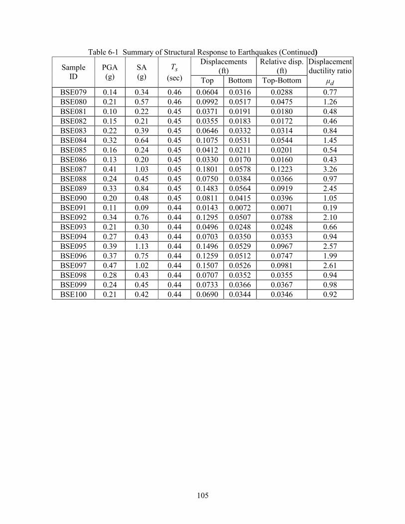
105

Table 6-1 Summary of Structural Response to Earthquakes (Continued) Displacements

(ft) Relative disp.

(ft) Sample ID

PGA (g)

SA (g)

sT (sec) Top Bottom Top-Bottom

Displacement ductility ratio

dµ BSE079 0.14 0.34 0.46 0.0604 0.0316 0.0288 0.77 BSE080 0.21 0.57 0.46 0.0992 0.0517 0.0475 1.26 BSE081 0.10 0.22 0.45 0.0371 0.0191 0.0180 0.48 BSE082 0.15 0.21 0.45 0.0355 0.0183 0.0172 0.46 BSE083 0.22 0.39 0.45 0.0646 0.0332 0.0314 0.84 BSE084 0.32 0.64 0.45 0.1075 0.0531 0.0544 1.45 BSE085 0.16 0.24 0.45 0.0412 0.0211 0.0201 0.54 BSE086 0.13 0.20 0.45 0.0330 0.0170 0.0160 0.43 BSE087 0.41 1.03 0.45 0.1801 0.0578 0.1223 3.26 BSE088 0.24 0.45 0.45 0.0750 0.0384 0.0366 0.97 BSE089 0.33 0.84 0.45 0.1483 0.0564 0.0919 2.45 BSE090 0.20 0.48 0.45 0.0811 0.0415 0.0396 1.05 BSE091 0.11 0.09 0.44 0.0143 0.0072 0.0071 0.19 BSE092 0.34 0.76 0.44 0.1295 0.0507 0.0788 2.10 BSE093 0.21 0.30 0.44 0.0496 0.0248 0.0248 0.66 BSE094 0.27 0.43 0.44 0.0703 0.0350 0.0353 0.94 BSE095 0.39 1.13 0.44 0.1496 0.0529 0.0967 2.57 BSE096 0.37 0.75 0.44 0.1259 0.0512 0.0747 1.99 BSE097 0.47 1.02 0.44 0.1507 0.0526 0.0981 2.61 BSE098 0.28 0.43 0.44 0.0707 0.0352 0.0355 0.94 BSE099 0.24 0.45 0.44 0.0733 0.0366 0.0367 0.98 BSE100 0.21 0.42 0.44 0.0690 0.0344 0.0346 0.92

106

107

108

SECTION 7

SEISMIC FRAGILITY ANALYSIS OF BRIDGE

The fragility curves of a bridge display the conditional probability that the structural demand

(structural response) caused by various levels of ground shaking exceeds the structural capacity

defined by a damage state. As shown in Table 4-19, the damage states used in this study are the

five damage states for bridges defined in the HAZUS99. In this study, the five damage states are

quantified in term of the relative displacement ductility ratios of bridge columns as shown in

Table 4-20.

In this study, the probabilistic characteristics of structural capacity are described by a lognormal

distribution.

cµ = Ln )~( β,µ cc (7-1)

where cµ is the median value of structural capacity and βc is the logarithmic standard

deviation. The median values corresponding to various displacement ductility ratios are taken as

those computed in Section 4 and are summarized in Table 7-1.

The probability that the structure demand dµ exceeds the structural capacity cµ can be

computed using the following formula.

fp' = Pr ≤d

cµµ( 1) (7-2)

Since both cµ and dµ follow the lognormal distribution, the probability of exceeding a specified

damage state fp' can be determined as follows:

109

fp' = ���

�

�

���

�

�

+

−

2122(

)~~

Ln(

)ββµ

µ

dc

dc

(7-3)

Following the recommendations in HAZUS99, )ββ( dc22 21

+ is taken as 0.4 when the fragility

curve is expressed in terms of SA. It is taken as 0.5 when the fragility curve is expressed in

terms of PGA. The fragility curves as a function of SA and PGA are shown in Figures 7-1 and

7-2, respectively.

110

Table 7-1 Median Structural Capacities Corresponding to Various Displacement Ductility Ratios

Displacement ductility ratio Median value

µcy1 1.00

µcy 1.20

µc2 1.76

µc max 4.76

111

112

113

SECTION 8

DISCUSSIONS AND CONCLUSIONS

This report presents an analytical method for developing seismic fragility curves of highway

bridges. In this method, appropriate models for seismic source, path attenuation, local site

condition, and bridge are established and used to simulate the response of bridge to earthquakes.

The uncertainties in the earthquake-site-bridge system are quantified by estimating uncertainties

in the pertinent parameters that are used to define the analytical models. The advantage of this

approach is that the assessment of uncertainties in these parameters can be easily verified and

refined. Several issues pertinent to the use of analytical methods for the development of seismic

fragility curves are discussed below.

Traditionally, the fragility curves of a structure are developed from random vibration analysis of

structures. The advantage of random vibration analysis is that the probabilistic characteristics of

structural response can be obtained analytically. However, random vibration analysis is most

useful for linear structures because the principle of superposition is utilized in the analysis. To

include nonlinear behavior of structures, the direct simulation is usually employed by performing

nonlinear seismic response analysis of structures. It is noted that the direct simulation has

become feasible in recent years because of the increase in computing power and storage

capacities of personal computers and microcomputers.

In direct simulation, the number of simulations is a critical consideration. For those structures

that can be represented by a model with a single degree of freedom or a few degrees of freedom,

the number of simulations is not a problem. However, for those structures that cannot be

represented by a simple structural model, for example, irregular buildings and curved bridges, a

realistic structural model like a finite element model needs to be employed and the number of

simulations is a critical consideration.

The choice of a parameter to represent the intensity of ground shaking is another consideration.

Traditionally, peak ground acceleration (PGA) is used as the ground shaking parameter for the

generation of fragility curves. The reason to use PGA as the ground shaking parameter is that it

114

is readily available from earthquake records. Thus, it is convenient to use PGA for the

development of fragility curves when the curves are derived empirically from earthquake

experience data. It is well known, however, that PGA is not a good measure of seismic demand

on a structure. In the simulation, when PGA is used as the ground shaking parameter, the

simulated structural response data are scattered and thus, the number of simulations needs to be

increased. Conversely, the simulated response data are less scattered when spectral acceleration

(SA) instead of PGA is used as the ground shaking parameter. However, it is difficult to apply

the fragility curves expressed in terms of SA to a large inventory of structures because the

determination of the fundamental periods of these structures is not trivial. Strictly speaking,

spectral acceleration is a structural parameter and is not really a ground shaking parameter.

Additional studies need to be conducted in order to find an appropriate pure ground shaking

parameter for the expression of structural responses and fragility curves.

In most seismic fragility analyses, the probabilistic structural demand is described by a

lognormal distribution. A lognormal distribution is defined by two parameters: the median value

and the logarithmic standard deviation. It is noted that the median value can be determined from

a few runs of simulation. On the other hand, a large number of simulation runs are required in

order to determine the logarithmic standard deviation. For the practical fragility analysis of a

complex structure, an overall logarithmic standard deviation may be used as recommended in

HAZUS99 to reduce the number of simulation runs.

The fragility curves of bridges can be used to estimate the chance that a bridge will be damaged

in a seismic event. In addition to fragility curves, the repair cost and the recovery time are also

required for evaluating the seismic performance of a highway system. In the central and eastern

United States, no data on the repair cost and recovery time are available because damaging

earthquakes are very scarce. One way to develop such a database is through the survey of expert

opinions. As an example, Hwang et al. (2000) have developed repair costs and recovery times

for various degrees of damage to a 602-11 bridge based on the survey of experts in the state

departments of transportation and consulting engineering companies.

115

SECTION 9

REFERENCES

Atkinson, G., and Mereu, R. (1992). �The Shape of Ground Motion Attenuation Curves in

Southern Canada.� Bulletin of the Seismological Society of America, 82, 2014-2031.

ATC 32: Improved Seismic Design Criteria for California Bridges: Provisional

Recommendations (1996). Applied Technology Council (ATC), Redwood City, CA.

Basoz, N., and Kiremidjian, A. (1998). Evaluation of Bridge Damage Data from the Loma Prieta

and Northridge, California Earthquakes. Technical Report MCEER-98-004,

Multidisciplinary Center for Earthquake Engineering Research, Buffalo, NY.

Boore, D.M. (1983). �Stochastic Simulation of High-frequency Ground Motions Based on

Seismological Models of the Radiation Spectra.� Bulletin of the Seismological Society of

America, 73, 1865-1894.

Boore, D.M., and Boatwright, J. (1984). �Average Body-Wave Radiation Coefficients.� Bulletin

of the Seismological Society of America, 74, 1615-1621.

Boore, D.M., and Joyner, W.B. (1991). �Estimation of Ground Motion at Deep-soil Sites in

Eastern North America.� Bulletin of the Seismological Society of America, 81, 2167-2185.

Boore, D.M. (1996). SMSIM � Fortran Programs for Simulating Ground Motions from

Earthquakes: Version 1.0. Open-File Report 96-80-A, U.S. Geological Survey, Menlo Park,

CA.

Brune, J.N. (1970). �Tectonic Stress and Spectra of Seismic Shear Waves from Earthquakes.�

Journal of Geophysical Research, 75, 4997-5009.

Brune, J.N. (1971). �Correction.� Journal of Geophysical Research, 76, 5002.

Chiu, J.M., Johnston, A., and Yang, Y.T. (1992). �Imaging the Active Faults of the Central New

Madrid Seismic Zone Using PANDA Array Data.� Seismological Research Letters, 63, 375-

394.

French, S.P., and Bachman, W.H. (1999). �Transportation facilities in Mid-America.�

Proceeding of the 5th U.S. Conference on Lifeline Earthquake Engineering, Seattle, WA,

August 12-14, 1999, 582-591.

Guidelines for Determining Design Basis Ground Motions (1993). EPRI TR-102293, Electric

Power Research Institute, Palo Alto, CA.

116

Hanks, T.C., and Kanamori, H. (1979). �A Moment Magnitude Scale.� Journal of Geophysics

Research, 84, 2348-2350.

Hanks, T.C., and McGuire, R.K. (1981). �The Character of High-Frequency Strong Ground

Motion.� Bulletin of the Seismological Society of America, 71, 2071-2095.

HAZUS99 User�s Manual (1999). Federal Emergency Management Agency, Washington, D.C.

Hwang, H., and Lee, C.S. (1991). �Parametric Study of Site Response Analysis.� Soil Dynamics

and Earthquake Engineering, 10(6), 382-290.

Hwang, H., and Huo, J.R.(1994). �Generation of Hazard-consistent Ground Motions.� Soil

Dynamics and Earthquake Engineering, 13(6), 377-386.

Hwang, H., and Huo, J.R. (1998). �Probabilistic Seismic Damage Assessment of

Highway Bridges.� Proceedings of the Sixth U.S. National Conference on Earthquake

Engineering, Seattle, WA, May 31-June 4, 1998, Earthquake Engineering Research Institute,

Oakland, CA (on CD-ROM).

Hwang, H., Jernigan, J.B., and Lin, Y.W. (1999). �Expected Seismic Damage to Memphis

Highway Systems.� Proceeding of the 5th U.S. Conference on Lifeline Earthquake

Engineering, Seattle, WA, August 12-14, 1999, 1-10.

Hwang, H., Jernigan, J.B., Billings, S., and Werner, S.D. (2000). �Expert Opinion Survey on

Bridge Repair Strategy and Traffic Impact.� Proceedings of the Post Earthquake Highway

Response and Recovery Seminar, St. Louis, MO, September 5-8, 2000. Federal Highway

Administration, Washington, D.C.

Idriss I.M. (1990). �Response of Soft Soil Sites During Earthquakes.� Proceedings of the H. B.

Seed Memorial Symposium, Berkeley, CA, 2, 273-289.

Idriss, I.M., and Sun, J.I. (1992). SHAKE91, a Computer Program for Conducting Equivalent

Linear Seismic Response Analyses of Horizontally Layered Soil Deposits, User�s Manual.

Center for Geotechnical Modeling, Department of Civil and Environmental Engineering,

University of California, Davis, CA.

117

Mander, J.B., Kim, D-K., Chen, S.S., and Premus, G.J. (1996). Response of Steel Bridge

Bearings to Reversed Cyclic Loading. Technical Report NCEER-96-0014, National Center

for Earthquake Engineering Research, State University of New York at Buffalo, NY.

Mander, J.B., and Basoz, N. (1999). �Seismic Fragility Curve Theory for Highway Bridges.�

Proceeding of the 5th U.S. Conference on Lifeline Earthquake Engineering, Seattle, WA,

August 12-14, 1999, 31-40.

Priestley, M.J.N., Seible, F., and Calvi, G.M. (1996). Seismic Design and Retrofit of Bridges.

John Wiley & Sons, Inc., New York, NY.

SAP2000, Integrated Finite Element Analysis and Design of Structures: Analysis Reference

(1996). Computers and Structures, Inc., Berkeley, CA.

Seismic Retrofitting Manual for Highway Bridges (1995). Publication No. FHWA-RD-94-052,

Office of Engineering and Highway Operations R&D, Federal Highway Administration,

McLean, VA.

Shinozuka, M. (2000). �Development of Bridge Fragility Curves Based on Damage Data.�

Proceedings of International Workshop on Annual Commemoration of Chi-Chi Earthquake,

September 18-20, 2000, Taipei, Taiwan, II, 14-25.

Vucetic, M., and Dobry, R. (1991). �Effect of Soil Plasticity on Cyclic Response.� Journal of

Geotechnical Engineering, 117 (GE1), 89-107.

Wallace, J.W. (1992). BIAX, A Computer Program for the Analysis of Reinforced Concrete and

Reinforced Masonry Sections. Report No. CU/CEE-92/4, Department of Civil Engineering,

Clarkson University, Potsdam, New York.