Segmentation of Textures Defined on Flat vs.

Layered Surfaces using Neural Networks:

Comparison of 2D vs. 3D Representations 1

Sejong Oh a,b Yoonsuck Choe a,∗

aDepartment of Computer Science, Texas A&M University,3112 TAMU, College Station, TX 77843-3112

bRepublic of Korea Airforce, Korea

Abstract

Texture boundary detection (or segmentation) is an important capability in humanvision. Usually, texture segmentation is viewed as a 2D problem, as the definitionof the problem itself assumes a 2D substrate. However, an interesting hypothesisemerges when we ask a question regarding the nature of textures: What are textures,and why did the ability to discriminate texture evolve or develop? A possible answerto this question is that textures naturally define physically distinct (i.e., occluded)surfaces. Hence, we can hypothesize that 2D texture segmentation may be an out-growth of the ability to discriminate surfaces in 3D. In this paper, we conductedcomputational experiments with artificial neural networks to investigate the rela-tive difficulty of learning to segment textures defined on flat 2D surfaces vs. those in3D configurations where the boundaries are defined by occluding surfaces and theirchange over time due to the observer’s motion. It turns out that learning is fasterand more accurate in 3D, very much in line with our expectation. Furthermore, ourresults showed that the neural network’s learned ability to segment texture in 3Dtransfers well into 2D texture segmentation, bolstering our initial hypothesis, andproviding insights on the possible developmental origin of 2D texture segmentationfunction in human vision.

Key words: Texture Segmentation, Neural Networks, 3D Surface Representation,Occlusion

∗ Corresponding author. Email: choe@tamu.edu.URL: http://faculty.cs.tamu.edu/choe.1 The authors wish to thank Ricardo Gutierrez-Osuna, Jay McClelland, PawanSinha, Takashi Yamauchi, and three anonymous reviewers for their valuable com-ments; and Jyh-Charn Liu for his support. Technical assistance by Yingwei Yu isalso greatly appreciated. This research was supported in part by the Texas Higher

1

1 Introduction

Detection of a tiger in the shrub is a perceptual task that carries a life ordeath consequence for preys trying to survive in the jungle [1]. Here, figure-ground separation becomes an important perceptual capability. Figure-groundseparation is based on many different cues such as luminance, color, texture,etc. In case of the tiger in the jungle, texture plays a critical role. What are thevisual processes that enable perceptual agents to separate figure from groundusing texture cues? This intriguing question led many researchers in vision toinvestigate the mechanisms of texture perception.

Beck [2][3] and Julesz [4] conducted psychological experiments investigatingthe features that enable humans to discriminate one texture from another.These studies suggested that texture segmentation occurs based on the dis-tribution of simple properties of “texture elements,” such as brightness, color,size, and the orientation of contours, or other elemental descriptors [5]. Juleszalso proposed the texton theory, in which textures are discriminated if theydiffer in the density of simple, local textural features, called textons [6]. Mostmodels based on these observations lead to a feature-based theory in whichsegmentation occurs when feature differences (such as difference in orienta-tion) exist. On the other hand, psychophysical and neurophysiological exper-iments have shown that texture processing may be based on the detection ofboundaries between textures using contextual influences via intra-cortical in-teractions in the visual cortex [7][8][9] (for computational models, see [10][11]).

In the current studies of texture segmentation and boundary detection, tex-ture is usually defined in 2D. However, an interesting hypothesis arises whenwe ask an important question regarding the nature of textures: What are tex-tures, and why did the ability to discriminate textures evolve or develop? Onepossible answer to the question is that texture is that which defines physicallydistinct (i.e., occluded or occluding) surfaces belonging to different objects,and that texture segmentation function may have evolved out of the neces-sity to distinguish between different surfaces. Human visual experience withtextures can be, therefore, in most cases to use them as cues for surface per-ception, depth perception, and 3D structure perception. In fact, psychologicalexperiments by Nakayama and He [12][13] showed that the visual system can-not ignore information regarding surface layout in texture discrimination andproposed that surface representation must actually precede perceptual func-tions such as texture perception (see the discussion section for more on thispoint).

From the discussion above, we can reasonably infer that texture processing

Education Coordinating Board grant ATP#000512-0217-2001 and the National In-stitute of Mental Health Human Brain Project grant #1R01-MH66991.

2

may be closely related to surface discrimination. Surface discrimination isfundamentally a 3D task, and 3D cues such as stereopsis and motion paral-lax may provide unambiguous information about the surface. Thus, we canhypothesize that 3D surface perception could have contributed in the forma-tion of early texture segmentation capabilities in human vision. In this paper,through computational experiments using artificial neural networks, we inves-tigated the relative difficulty of learning to discriminate texture boundariesin 2D vs. 3D arrangements of texture. In the 2D arrangement, textures areshown on a flat 2D surface, whereas in the 3D counterpart they are shownas patterns on two surfaces, one occluding the other which also appears toslide due to the motion of the observer. We will also evaluate whether thelearned ability to segment texture in 3D can transfer into 2D. In the follow-ing, we will first describe in detail the methods we used to prepare the 2D andthe 3D texture inputs (Section 2.1), and the procedure we followed to trainmultilayer perceptrons to discriminate texture boundaries (Section 2.2). Next,we will present our main results and interpretations (Section 3), followed bydiscussion (Section 4) and conclusion (Section 5).

2 Methods

To test our hypothesis proposed in the introduction, we need to conduct tex-ture discrimination experiments with 2D and 3D arrangements of texture.In this section, we will describe in detail how we prepared the two differentarrangements (Section 2.1), and explain how we trained two standard multi-layer perceptrons to discriminate these texture arrangements (Section 2.2).We trained two separate networks that are identical in architecture, one withinput prepared in a 2D arrangement (we will refer to this network as the2D-net), and the other with inputs in a 3D arrangement (the 3D-net).

2.1 Input preparation

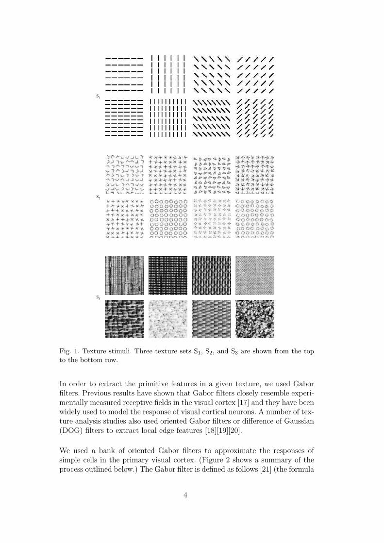
We used three sets of texture stimuli S1, S2, and S3 for our experiments (Fig-ure 1). Textures in S1 were simple artificial texture images (oriented bars oforientation 0, π

4, π

2, or 3π

4at two different spatial frequencies); those in S2 were

more complex texture images such as crosses and circles, adapted from Krose[14] and Julesz [15]; and those in S3 were real texture images from the widelyused Brodatz texture collection [16]. For the training of the 2D-net and the3D-net, the eight simple texture stimuli in S1 were used. For testing the per-formance of the 2D-net and the 3D-net, all sets of texture stimuli (S1, S2 andS3) were used.

3

S1

S2

S3

Fig. 1. Texture stimuli. Three texture sets S1, S2, and S3 are shown from the topto the bottom row.

In order to extract the primitive features in a given texture, we used Gaborfilters. Previous results have shown that Gabor filters closely resemble experi-mentally measured receptive fields in the visual cortex [17] and they have beenwidely used to model the response of visual cortical neurons. A number of tex-ture analysis studies also used oriented Gabor filters or difference of Gaussian(DOG) filters to extract local edge features [18][19][20].

We used a bank of oriented Gabor filters to approximate the responses ofsimple cells in the primary visual cortex. (Figure 2 shows a summary of theprocess outlined below.) The Gabor filter is defined as follows [21] (the formula

4

*

Rii=1..4, j=1..3max Riargmax

i=1..4, j=1..3

i

Riargmaxi=1..4, j=1..3

j

ij

I

convolution

full−wave rect.

Cij

R ij

Gabor Energy Orientation Spatial Frequency

Gi=

1..4

j=1..3

Fig. 2. Gabor filter bank. The process used to generate feature matrices is shown.The texture I is first convolved with the Gabor filters Gij (for i = 1..4, j = 1..3),and the resulting responses are passed through a full-wave rectifier resulting in Rij .Finally, we obtain the Gabor energy matrix Eij , orientation index matrix Oij , andfrequency index matrix Fij .

below closely follows [22]):

Gθ,φ,σ,ω(x, y) = exp−x′2+y′2

σ2 cos (2πωx′ + φ) , (1)

where θ is the orientation, φ the phase, σ the standard deviation (width) ofthe Gaussian envelope, ω the spatial frequency, (x, y) the pixel location, andx′ and y′ defined as:

x′ = x cos(θ) + y sin(θ), (2)

y′ =−x sin(θ) + y cos(θ). (3)

The size of the filter was 16 × 16 (n × n where n = 16). For simplicity,only four different orientations, 0, π

4, π

2, and 3π

4, were used for θ. (Below, we

will refer to Gθ,φ,σ,ω as simply G.) The phase of the cosine was φ = π2, and

the Gaussian envelope width was σ = n2. To adequately sample the spatial-

frequency features of the input stimuli, three frequencies, 1n, 2

n, and 3

n, were

used for ω. This resulted in 12 filters Gij, where the index over orientations was

i = 1..4(θ = (i−1)π

4

), and that over spatial frequencies j = 1..3

(ω = j

n

). To

5

get the Gabor response matrix Cij for orientation index i and spatial frequencyindex j, a gray-level intensity matrix I was obtained from the images randomlyselected from S1 and convolved with the filter bank Gij:

Cij = I ∗ Gij, (4)

where i = 1..4 and j = 1..3 denote the orientation and spatial frequencyindices of the filters in the filter bank, and ∗ represents the convolution op-erator. The Gabor filtering stage is linear, but models purely based on linearmechanisms are not able to reproduce experimental data [23]. Thus, half-waverectification is commonly used to provide a nonlinear response characteristicfollowing linear filtering. However, in our experiments, full-wave rectificationwas used as in [24], which is similar to half-wave rectification, but is simplerto implement. Full-wave rectification is equivalent to summing the outputs ofthe two corresponding half-wave rectification channels (see, e.g. Bergen andAdelson [25] [23]). The final full-wave rectified Gabor feature response matrixis calculated as

Rij = |Cij|, (5)

for i = 1..4 and j = 1..3, where | · | represents the element-wise absolute valueof the matrix.

For each sample texture pair, we acquired three response matrices: the Gaborenergy matrix E, the orientation index matrix O, and the frequency indexmatrix F . The E matrix simply indicates the “edgyness” at each point, whichis analogous to the orientation selectivity in primary visual cortical (V1) neu-rons [26]. On the other hand, O indicates which orientation is most prominentat each point, which again has an analog in neurophysiology: the orientationpreference in V1 neurons [26]. Finally, F represents how fine the spatial featureis at each point, for which its neural mechanism is also known [27]. Thus, theselection of these three features are consistent with known neurophysiology ofV1.

The Gabor energy response matrix E was defined as follows:

E(x, y) = maxi=1..4,j=1..3

Rij(x, y), (6)

where (x, y) is the location in each matrix, and i and j are the orientationand spatial frequency indices, and Rij the response matrix (Equation 5). Theorientation index matrix O and the frequency index matrix F were calculatedas

(O(x, y), F (x, y)) = arg maxi=1..4,j=1..3

Rij(x, y), (7)

6

(a) Texture with boundary (b) Response to (a)

0.5 0.75

1

E

E

0.25 0.5

0.75 1

O

O

0 0.25

0.5 0.75

1

0 5 10 15 20 25 30 35

F

Position

F

0.25 0.5

0.75 1

E

E

0.5

0.75

1

O

O

0 0.25

0.5 0.75

1

0 5 10 15 20 25 30 35

F

Position

F

(c) Response profile of (b) (d) Response profile (“no boundary”)

Fig. 3. Generating the 2D input set. The procedure used to generate the 2D trainingdata is shown. (a) Input with a texture boundary. (b) Orientation response calcu-lated from (a). Only the E matrix is shown. The 32-pixel wide line marked in whiteindicates where an input vector was sampled. (c) The response profile from the32-pixel wide area marked with a white rectangle in (b). The three curves representthe profiles in the E, O, and F matrices. (d) A similarly calculated response pro-file in a different input texture, for an area without a texture boundary (note theidentical periodic peaks, unlike in (c)).

where arg max(·) is a vector valued function which returns two indices i andj where Rij(x, y) is the maximum, one for orientation and one for spatial fre-quency, which are subsequently assigned to O(x, y) and F (x, y), respectively.Finally, each matrix was independently normalized by dividing with its max-imum value. Figure 2 shows the Gabor filter bank and the three matrices E,O, and F of the given texture pair.

To get the 2D training samples for the 2D-net, two randomly selected texturesfrom S1 were paired side-by-side and convolved with the Gabor filter bank(Figure 2). The E, O, and F matrices were then obtained using Equations 6and 7, and then normalized as explained above.

Each training input in the 2D training set consisted of three 32-element vectorstaken from a horizontal strip from the E, O, and F matrices (Figure 3b,showing E, marked white). Each horizontal strip had a width of 32, and wastaken from the center of the matrix where the two textures meet, with avarying y location randomly chosen where the E sum in that row exceededthe mean row sum of E for that particular texture (Figure 3b). The threevectors were pasted to form a 96-element vector ξ2D

k , where k represents thetraining sample index, and the superscript 2D denotes that this vector is in the2D set. Finally, the target ζ2D

k was set either to 0 (for “no border” condition)

7

or to 1 (for “border” condition), thus giving an input-target pair (ξ2Dk , ζ2D

k ) forthe 2D case. Examples of these three 32-element vectors are shown in Figure 3c(texture with boundary), and in Figure 3d (texture without boundary).

In order to generate samples for the 3D-net, occlusion cue generated from self-motion was used as shown in Figure 4. One texture from a pair of texturesoccluded the other where the texture above was allowed to slide over theother, which resulted in successive further occlusion of the texture below. Theoccluding texture above was moved by one pixel at a time 32 times and eachtime the resulting 2D image (I ′t, for t = t1...t32; Figure 5a) was convolved withthe oriented Gabor filter bank followed by full-wave rectification as in the2D case (Figure 5b). To generate a single training input-target pair (ξ3D

k , ζ3Dk )

for the 3D-net, at each time step the Gabor energy response value E(xc, yc),orientation response value O(xc, yc) and frequency response value F (xc, yc)were separately collected into three 32-element vectors, where xc was 16 pixelsaway to the right from the initial texture boundary in the middle, and yc wasselected randomly as in the 2D case (the white squares in Figure 5b). Finally,the three 32-element vectors were pasted to form a 96-element vector ξ3D

k .Figure 5c shows examples of ξ3D

k (note that the x-axis represents time, unlikein the 2D case where it is spatial position: see the discussion section for more onthis point) for a case containing a texture boundary, and Figure 5d for a casewithout a boundary. The target value ζ3D

k of the input-target pair (ξ3Dk , ζ3D

k )was set in a similar manner as in the 2D case, either to 0 (no boundary) orto 1 (boundary). When collecting the training samples for the 3D-net wherethere was a texture boundary, the above procedure was performed with twodifferent 3D configurations. In the first configuration, the texture on the leftside was on top of the texture on the right side with self-motion of observerfrom right to left. In the second configuration, the texture on the right wason top of the texture on the left side with self-motion of observer from left toright. For an unbiased training set, the same number of samples were collectedfor each 3D configuration. The “no boundary” condition was identical to the2D case without a boundary, since no texture boundary in 3D means oneuniform texture over a single surface.

For both the 2D and the 3D arrangements, texture patches were uniformlyrandomly sampled to form a texture pair, and 2,400 “boundary” and 2,400“no boundary” cases were generated for each arrangement. This resulted in4,800 input-target samples for each training set.

2.2 Training the texture segmentation networks

We used standard multilayered perceptrons (MLPs) to perform texture bound-ary detection. The networks (2D-net and 3D-net), which consisted of two layers

8

32 1t t

... ...

t32

t1

t2

(a) Texture in 3D (b) Resulting 2D view

Fig. 4. Generating the 3D input set. (a) A 3D configuration of textures and (b)the resulting 2D views before, during, and after the movement are shown. As theviewpoint is moved from the right to the left (t1 to t32) in 32 steps, the 2D textureboundaries in (b) (marked by black arrows) show a subtle variation.

including 96 input units, 16 hidden units and, 2 output units, were trainedfor 2,000 epochs each using standard backpropagation (see e.g., [28]) 2 . Thetarget outputs were set to (1, 0) for the “boundary” case, and (0, 1) for the“no boundary” case. The goal of this study was to compare the relative learn-ability of the 2D vs. the 3D texture arrangements, thus a backpropagationnetwork was good enough for our purpose. The hyperbolic tangent function(f(v) = tanh(v)) was used as the activation function of the hidden layer. Forthe activation function of the output layer, radial basis function (RBF) wasused (φ(v) = exp(−v2)). The use of the radial basis function in standard MLPis not common: It is usually used as an activation function of the hidden layerin radial basis function networks, which has additional data-independent in-put to the output layer. In the experiment, as shown in the previous section,an input vector to the MLP is symmetric about the center when there is noboundary. On the other hand, an input vector to the MLP is quite asymmetricwhen there is a boundary, but the mirror image of that vector should result inthe same class. This observation led us to use the radial basis function, whichhas a Gaussian profile. Several preliminary training trials showed that the useof the RBF as the activation function enabled both the 2D-net and the 3D-netto converge faster (data not shown here). For the training, the input vectorswere generated from the texture set S1. Backpropagation with momentum andadaptive learning rate was applied to train the weights.

To determine the best learning parameters, several preliminary training runswere done with combinations of learning rate parameters η ∈ {0.01, 0.1, 0.5}and momentum constants α ∈ {0.0, 0.5, 0.9}. MLPs with each combination

2 Matlab neural networks toolbox was used for the simulations.

9

1

32

2

t

t

t

Tim

e

... ... ...

(a) Input over time (b) Response to (a)

0.25 0.5

0.75 1

E

E

0.25 0.5

0.75 1

O

O

0 0.25

0.5 0.75

1

0 5 10 15 20 25 30 35

F

Time

F

0.5 0.75

1

E

E

0.75

1

O

O

0 0.25

0.5 0.75

1

0 5 10 15 20 25 30 35

F

Time

F

(c) Temporal profile of (b) (d) Temporal profile (no boundary)

Fig. 5. Generating 3D input set through motion. (a) Texture pair images resultingfrom simulated motion: I ′t for each t = t1..t32. (b) The response matrix of the texturepair: R3D

ij . The location sampled for the input vector construction is marked asa white square in each frame. (c) Response profile obtained over time near theboundary of two different texture images (marked by the small white squares in b).Take note of the flatness of the profile on the left half of the plots, which is quitedifferent from the 2D case. (d) A similarly measured response profile collected overtime, using a different input texture, near a location without a texture boundary(note the periodic peaks).

were trained with the same set of inputs so that the results of the experi-ment can be directly compared. Each training set consisted of 280 examples,drawn from S1 and processed by the input preparation procedure. The train-ing process continued for 1,000 epochs. The MLPs with other combination ofparameters failed to converge. Based on these preliminary training tests, wechose the learning parameters as follows: learning rate η = 0.01, and momen-tum constant α = 0.5.

We also applied standard heuristics to speed up and stabilize the convergenceof the networks. First, each input vector was further normalized so that its

10

vector mean, averaged over the entire training set, is zero. Secondly, adaptivelearning rate was applied. For each epoch, if the mean squared error (MSE)decreased toward the goal (10−4), then the learning rate (η) was increased bythe factor of ηinc:

ηn = ηn−1ηinc, (8)

where n is the epoch. If MSE increased by more than a factor of 1.04, thelearning rate was adjusted by the factor of ηdec:

ηn = ηn−1ηdec. (9)

The learning constants selected above (η = 0.01, α = 0.5) were used for thesecond test training to choose the optimal adaptive learning rate factors (ηinc

and ηdec). Combinations of the factors ηinc ∈ {1.01, 1.05, 1.09} and ηdec ∈{0.5, 0.7, 0.9} were used during the test training to observe their effects onconvergence. The combination of factors ηinc = 1.01 and ηdec = 0.5 werechosen based on these results.

After the training of the two networks, the speed of convergence and the clas-sification accuracy were compared. To test generalization and transfer poten-tials, test stimuli drawn from the texture sets S1, S2, and S3 were processedusing both 2D- and 3D input preparation methods to obtain six test inputsets (each with 4,800 inputs). These input samples were then presented to the2D-net and the 3D-net to compare the performances of the two networks onthese six test input sets. The results from these experiments will be presentedin the following section.

3 Experiments and Results

We compared the performance of the two trained networks (2D-net and 3D-net), and also compared the performance of the two networks over novel tex-ture images that were not used in training the networks.

3.1 Speed of convergence and accuracy on the training set

Figure 6 shows the learning curves of the networks during training. The learn-ing processes continued for 2,000 epochs. After 2,000 epochs, the average meansquared error (MSE) of the 2D-net was 0.0006 and that of the 3D-net was0.0003. The learning curve also shows that the 3D-net converges faster than

11

1e-04

0.001

0.01

0.1

1

0 500 1000 1500 2000

log

(MS

E)

Epoch

2D-net3D-net

Fig. 6. Learning curves of the networks. The learning curves of the 2D-net and the3D-net up to 2,000 epochs of training on texture set S1 are shown. The 3D-netis more accurate and converges faster than the 2D-net (the 3D-net reaches theasymptotic value of the 2D-net near 750 epochs), suggesting that the 3D-processedtraining set is easier to learn than the 2D set.

the 2D-net. The class response of the network was determined by finding whichoutput node (among the two) had the higher value. If the first output neu-ron had a greater response than the second, the classification was deemed tobe “boundary,” and otherwise “no boundary.” The misclassification rate wascomputed based on the comparison of this classification response against thetarget value (ζ). The misclassification rate for the 2D-net was 0.3%, and forthe 3D-net, 0.02%. In summary, the network learned texture arrangementsrepresented in 3D faster and more accurately than those in 2D.

3.2 Generalization and transfer (I)

The 2D-net and the 3D-net trained with the texture set S1 were tested ontexture pairs from S1, S2 and S3. (Note that for the texture set S1, inputsamples different from those in the training set were used.) The input setswere prepared in the same manner as the training samples (Section 2.1). All6 sample sets (= 3 texture sets × 2 representations) were presented to the2D-net and the 3D-net. Two methods to compare the performance of thenetworks were used. First, we compared the misclassification rate, which isthe percentage of misclassification. Misclassification rates were calculated forall 12 cases (= 6 sample sets × 2 networks): Figure 7 shows the result. The3D-net outperformed the 2D-net in all cases, except for the sample set fromS1 with 2D input processing, which was similar to those used for training the

12

0

10

20

30

40

50

60

70

S33DS32DS23DS22DS13DS12D

Misc

lass

ificat

ion

Rate

(%)

Test Set

2D-net3D-net

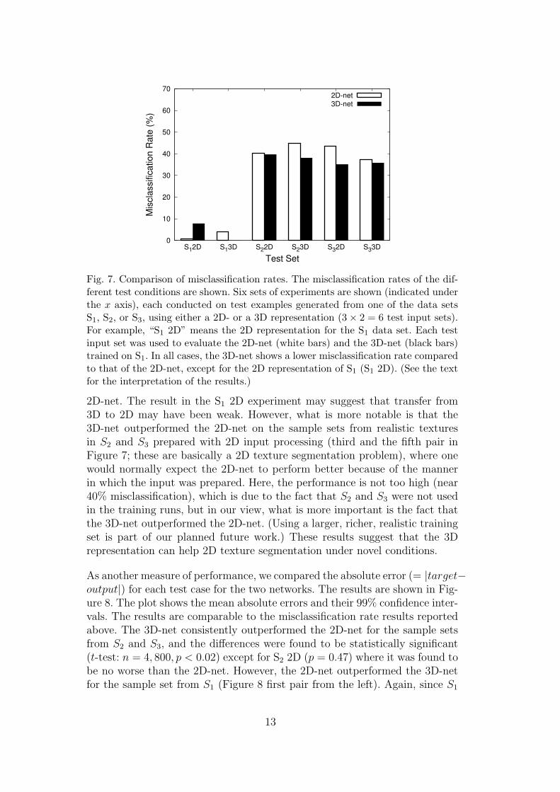
Fig. 7. Comparison of misclassification rates. The misclassification rates of the dif-ferent test conditions are shown. Six sets of experiments are shown (indicated underthe x axis), each conducted on test examples generated from one of the data setsS1, S2, or S3, using either a 2D- or a 3D representation (3 × 2 = 6 test input sets).For example, “S1 2D” means the 2D representation for the S1 data set. Each testinput set was used to evaluate the 2D-net (white bars) and the 3D-net (black bars)trained on S1. In all cases, the 3D-net shows a lower misclassification rate comparedto that of the 2D-net, except for the 2D representation of S1 (S1 2D). (See the textfor the interpretation of the results.)

2D-net. The result in the S1 2D experiment may suggest that transfer from3D to 2D may have been weak. However, what is more notable is that the3D-net outperformed the 2D-net on the sample sets from realistic texturesin S2 and S3 prepared with 2D input processing (third and the fifth pair inFigure 7; these are basically a 2D texture segmentation problem), where onewould normally expect the 2D-net to perform better because of the mannerin which the input was prepared. Here, the performance is not too high (near40% misclassification), which is due to the fact that S2 and S3 were not usedin the training runs, but in our view, what is more important is the fact thatthe 3D-net outperformed the 2D-net. (Using a larger, richer, realistic trainingset is part of our planned future work.) These results suggest that the 3Drepresentation can help 2D texture segmentation under novel conditions.

As another measure of performance, we compared the absolute error (= |target−output|) for each test case for the two networks. The results are shown in Fig-ure 8. The plot shows the mean absolute errors and their 99% confidence inter-vals. The results are comparable to the misclassification rate results reportedabove. The 3D-net consistently outperformed the 2D-net for the sample setsfrom S2 and S3, and the differences were found to be statistically significant(t-test: n = 4, 800, p < 0.02) except for S2 2D (p = 0.47) where it was found tobe no worse than the 2D-net. However, the 2D-net outperformed the 3D-netfor the sample set from S1 (Figure 8 first pair from the left). Again, since S1

13

0

0.1

0.2

0.3

0.4

0.5

0.6

S33DS32DS23DS22DS13DS12D

Mea

n|Er

ror|+

/-99%

Con

f. In

t.

Test Set

2D-net3D-net

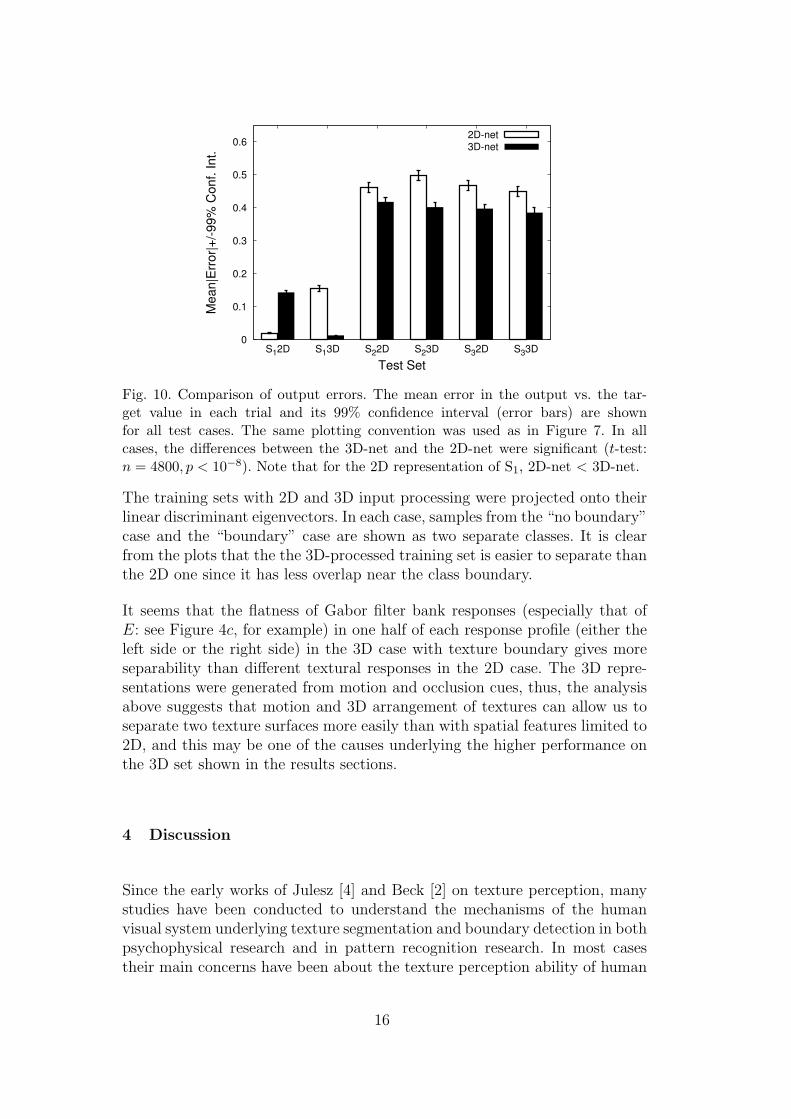
Fig. 8. Comparison of output errors. The mean error in the output vs. the targetvalue in each trial and its 99% confidence interval (error bar) are shown for all testcases (the plotting convention is the same as Figure 7). In all cases, the differencesbetween the 3D-net and the 2D-net were significant (t-test: n = 4, 800, p < 0.02),except for S2 2D (p = 0.47) where the performance was comparable. Note that forthe 2D representation of S1, 2D-net < 3D-net.

processed in 2D was used for training the 2D-net (although the samples weredifferent), this was expected from the beginning.

3.3 Generalization and transfer (II)

The main goal of our work was to understand the nature of textures, andfrom that emerged the importance of 3D cues in understanding the texturedetection mechanism in human visual processing. To emulate 3D depth, weemployed motion cues to provide depth. This imposes potential limitations onour work, which is that additional information in 3D input may have becomeavailable to the 3D-net; some form of temporal information that 2D inputsdoes not have. For example, in the 3D case, sliding of one texture over anotherproduces richer local textures near the boundary than in the 2D case, wherethe boundary has a fixed local texture. This can be seen as an unfair advantagefor the 3D-net. One way of addressing this issue may be to normalize (orequalize) the information content in the 2D vs. the 3D input preparation,which may allow us to more fairly assess the differences between the twomodes of texture processing. This can be done by generating 2D textures byaltering their overlap location rather than always putting them together inthe center.

We conducted an identical set of experiments described in the previous sectionswith the only difference being the difference in the 2D input set preparation.

14

0

10

20

30

40

50

60

70

S33DS32DS23DS22DS13DS12D

Misc

lass

ificat

ion

Rate

(%)

Test Set

2D-net3D-net

Fig. 9. Comparison of misclassification rates. The misclassification rates of the dif-ferent test conditions are shown (the plotting convention is the same as Figure 7).In all cases, the 3D-net shows a lower misclassification rate compared to that of the2D-net, except for the 2D representation of S1.

We used the same procedure prescribed in Section 2.1, except that the 2Dtexture boundary in the middle was made by allowing the texture boundaryto be defined not only by abutting the two input patches side-by-side, but alsoby slightly overlapping one over the other as in Figure 4b (but on the sameflat plane). The amount of overlap was randomly varied from 0 to 32 in thehorizontal direction.

The misclassification rate and MSE results are shown in Figures 9 and 10. Theresults are consistent with (or, even stronger than) the previous results. Aninteresting observation is that the performance of the 2D-net became worse,which is somewhat counter to our expectations given our rational for conduct-ing this experiment provided earlier in this section. Our observation is thatthe added variety of the possible combination of texture features near theboundary resulted in the increase in the number of representative patterns toclassify as “boundary,” thus the network had a harder time learning all thesedifferent characteristic patterns (i.e., there were too many equivalence classesto learn). In summary, the results presented here and in the previous sectionsupport our main hypothesis.

3.4 Separability of 2D vs. 3D representations

In order to better understand the reason why the 3D representation is supe-rior to its 2D counterpart, we analyzed the two representations using LinearDiscriminant Analysis (LDA; see e.g., [29]). Figure 11 shows the results onrepresentations drawn from input data set S1.

15

0

0.1

0.2

0.3

0.4

0.5

0.6

S33DS32DS23DS22DS13DS12D

Mea

n|Er

ror|+

/-99%

Con

f. In

t.

Test Set

2D-net3D-net

Fig. 10. Comparison of output errors. The mean error in the output vs. the tar-get value in each trial and its 99% confidence interval (error bars) are shownfor all test cases. The same plotting convention was used as in Figure 7. In allcases, the differences between the 3D-net and the 2D-net were significant (t-test:n = 4800, p < 10−8). Note that for the 2D representation of S1, 2D-net < 3D-net.

The training sets with 2D and 3D input processing were projected onto theirlinear discriminant eigenvectors. In each case, samples from the “no boundary”case and the “boundary” case are shown as two separate classes. It is clearfrom the plots that the the 3D-processed training set is easier to separate thanthe 2D one since it has less overlap near the class boundary.

It seems that the flatness of Gabor filter bank responses (especially that ofE: see Figure 4c, for example) in one half of each response profile (either theleft side or the right side) in the 3D case with texture boundary gives moreseparability than different textural responses in the 2D case. The 3D repre-sentations were generated from motion and occlusion cues, thus, the analysisabove suggests that motion and 3D arrangement of textures can allow us toseparate two texture surfaces more easily than with spatial features limited to2D, and this may be one of the causes underlying the higher performance onthe 3D set shown in the results sections.

4 Discussion

Since the early works of Julesz [4] and Beck [2] on texture perception, manystudies have been conducted to understand the mechanisms of the humanvisual system underlying texture segmentation and boundary detection in bothpsychophysical research and in pattern recognition research. In most casestheir main concerns have been about the texture perception ability of human

16

2

4

6

8

10

12

-0.6 -0.4 -0.2 0 0.2 0.4 0.6

Sam

ple

Inde

x (x

100)

LD

2

4

6

8

10

12

-0.6 -0.4 -0.2 0 0.2 0.4 0.6

Sam

ple

Inde

x (x

100)

LD

(a) LDA Projection of 2D Data (b) LDA Projection of 3D Data

0

1

2

3

4

5

6

7

8

-0.6 -0.4 -0.2 0 0.2 0.4 0.6

Pro

babi

lity

Den

sity

LD

BorderNo Border

0

1

2

3

4

5

6

7

8

-0.6 -0.4 -0.2 0 0.2 0.4 0.6

Pro

babi

lity

Den

sity

LD

BorderNo Border

(c) Prob. Density of 2D LDA Data (d) Prob. Density of 3D LDA Data

Fig. 11. Comparison of Linear Discriminant Analysis (LDA) Projection of 2D- and3D-processed Data. The LDA projections for the 2D- and the 3D-processed data areshown. (Only half the dataset, 1,200 in each class for each representation, is shownto avoid clutter.) (a) LDA projection of the 2D training set is shown. The x andthe y axes represent the linear discriminant axis and the input sample index. Eachinput sample is plotted either as “•” (for “border”) or “×” (for “no border”). Thetwo classes overlap over a large region in the middle. (b) The same, as in (a), for the3D training set is shown. The overlap region is much smaller than in (a). (c) Theprobability density along the linear discriminant eigenvector projection (projectiononto the x-axis in a) is shown for the 2D training set. The “border” case is plottedas a solid curve, and the “no border” case as a dotted curve. There is a large overlapnear 0. (d) The same, as in (c), for the 3D training set is shown. The overlappingarea in the middle is much smaller than in (c).

in 2D. The work presented in this paper suggests an alternative approach tothe problem of texture perception, with a focus on boundary detection. First,we demonstrated that texture boundary detection in 3D is easier than in 2D.We also showed that the learned ability to find texture boundary in 3D caneasily be transferred to texture boundary detection in 2D. Based on theseresults, our careful observation is that the outstanding ability of 2D textureboundary detection of the human visual system may have been derived froman analogous ability in 3D.

Our results allow us to challenge one common notion that many other textureboundary detection studies share. In that view, intermediate visual processingsuch as texture perception, visual search and motion process do not require ob-

17

FeaturesImage

PerceptionTexture

Visual Search

MotionPerception

(a) Traditional view

PerceptionTexture

Visual Search

MotionPerception

SurfaceRepresentationFeatures

Image

(b) An alternative view

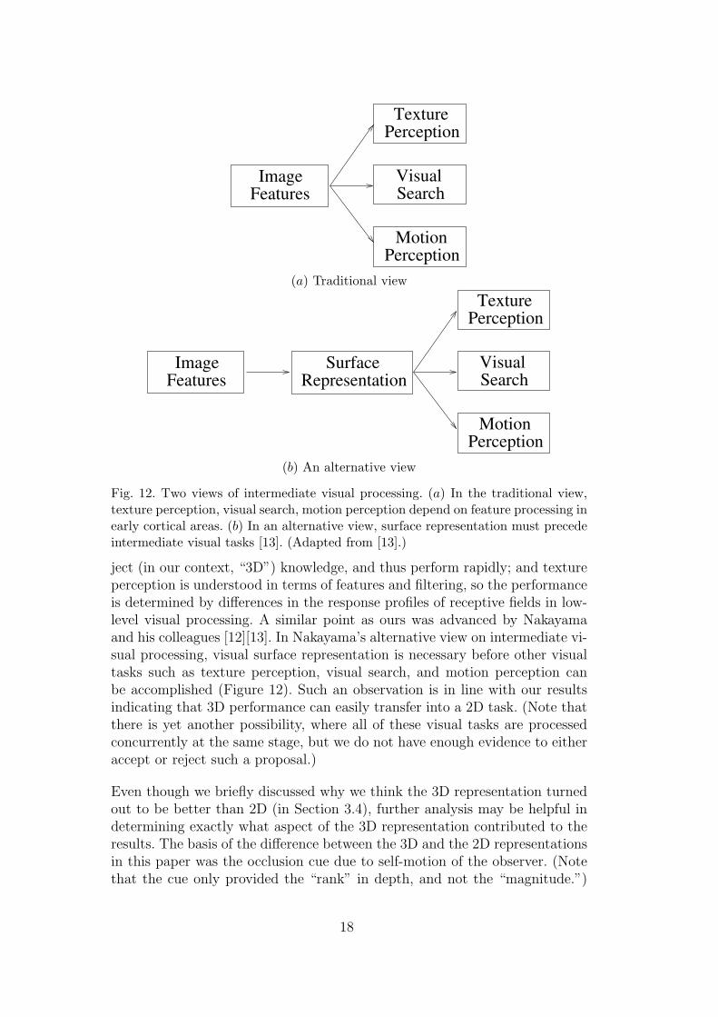
Fig. 12. Two views of intermediate visual processing. (a) In the traditional view,texture perception, visual search, motion perception depend on feature processing inearly cortical areas. (b) In an alternative view, surface representation must precedeintermediate visual tasks [13]. (Adapted from [13].)

ject (in our context, “3D”) knowledge, and thus perform rapidly; and textureperception is understood in terms of features and filtering, so the performanceis determined by differences in the response profiles of receptive fields in low-level visual processing. A similar point as ours was advanced by Nakayamaand his colleagues [12][13]. In Nakayama’s alternative view on intermediate vi-sual processing, visual surface representation is necessary before other visualtasks such as texture perception, visual search, and motion perception canbe accomplished (Figure 12). Such an observation is in line with our resultsindicating that 3D performance can easily transfer into a 2D task. (Note thatthere is yet another possibility, where all of these visual tasks are processedconcurrently at the same stage, but we do not have enough evidence to eitheraccept or reject such a proposal.)

Even though we briefly discussed why we think the 3D representation turnedout to be better than 2D (in Section 3.4), further analysis may be helpful indetermining exactly what aspect of the 3D representation contributed to theresults. The basis of the difference between the 3D and the 2D representationsin this paper was the occlusion cue due to self-motion of the observer. (Notethat the cue only provided the “rank” in depth, and not the “magnitude.”)

18

However, self-motion induces a more complex effect known as motion parallax,which not only gives occlusion cues but also relative difference in displacement(or relative speed) of the objects in the scene as a function of the distance ofthe observer from those objects [30]. We would like to clarify that our results,even though they are based on self-motion, do not account for (or utilize)the relative speed cue present in motion parallax. An important point hereis that there is a much richer set of information in 3D than the simplisticocclusion cue used in our model, and that the use of such extra information(also including stereo cues) may further assist in texture segmentation. These3D cues carry the most important piece of information, that “these two patchesof patterns are different,” thus providing the initial basis of discriminability(i.e., a supervisor signal) in texture segmentation.

Also, as pointed out in the text (Section 2.1), the 3D representations we gen-erated (the 96-element vectors) is defined over time, as opposed to the 2Dones defined over space. How is it possible that generalization can happenacross such seemingly incompatible representations? One clue can be found inspatiotemporal receptive fields in the visual pathway (e.g., in the lateral genic-ulate nucleus: [31]). These LGN neurons not only respond to spatial patternsbut also to patterns defined over time which have temporal profiles similarto the spatial profiles. It is tempting to speculate that these spatiotemporalreceptive fields may hold key to relating the transfer effect exhibited by ourneural network model to texture segmentation in humans. Also, this line ofreasoning suggests that it may be productive to investigate the role of motioncenters in the visual pathway (such as MT) in texture segmentation.

Finally, one potential criticism may be that we only used S1 for training. Woulda contradictory result emerge if S2 or S3 was used to train the networks? We arecurrently investigating this issue as well, but we are confident that our mainconclusion in this paper will hold even in such different training scenarios.

5 Conclusion

We began with the simple question regarding the nature of textures. Thetentative answer was that textures naturally define distinct physical surfaces,and thus the ability to segment texture in 2D may have grown out of theability to distinguish surfaces in 3D. To test our insight, we compared textureboundary detection performance of two neural networks trained on texturesarranged in 2D or in 3D. Our results revealed that texture boundary detectionin 3D is easier to learn than in 2D, and that the network trained in 3D solvedthe 2D problem better than the other way around. Based on these results,we carefully conclude that the human ability to segment texture in 2D mayhave originated from a module evolved to handle 3D tasks. One immediate

19

future direction is to extend our current approach to utilize stereo cues and fullmotion parallax cues as well as monocular occlusion cues used in this paper.

References

[1] M. Tuceryan, Texture analysis, in: The Handbook of Pattern Recognition andComputer Vision, 2nd Edition, World Scientific, Singapore, 1998, pp. 207–248.

[2] J. Beck, Effect of orientation and of shape similarity on grouping, Perceptionand Psychophysics 1 (1966) 300–302.

[3] J. Beck, Textural segmentation, second-order statistics and textural elements,Biological Cybernetics 48 (1983) 125–130.

[4] B. Julesz, Texture and visual perception, Scientific American 212 (1965) 38–48.

[5] M. S. Landy, N. Graham, Visual perception of texture, in: L. M. Chalupa, J. S.Werner (Eds.), The Visual Neurosciences, MIT Press, Cambridge, MA, 2004,pp. 1106–1118.

[6] B. Julesz, J. Bergen, Texton theory of preattentive vision and textureperception, Journal of the Optical Society of America 72 (1982) 1756.

[7] H. C. Nothdurft, Orientation sensitivity and texture segmentation in patternswith different line orientation, Vision Research 25 (1985) 551–560.

[8] H. C. Nothdurft, Feature analysis and the role of similarity in preattentivevision, Vision Research 52 (1992) 355–375.

[9] V. A. Lamme, V. Rodriguez-Rodriguez, H. Spekreijse, Separate processingdynamics for texture elements, boundaries and surfaces in primary visual cortexof the Macaque monkey, Cerebral Cortex 9 (1999) 406–413.

[10] A. Thielscher, H. Neumann, Neural mechanisms of cortico-cortical interactionin texture boundary detection: a modeling approach, Neuroscience. 122 (2003)921–939.

[11] Z. Li, Pre-attentive segmentation in the primary visual cortex, Spatial Vision13 (2000) 25–50.

[12] Z. J. He, K. Nakayama, Perceiving textures: Beyond filtering, Vision Research34 (1994) 151–62.

[13] K. Nakayama, Z. J. He, S. Shimojo, Visual surface representation: A critical linkbetween lower-level and higher-level vision, in: S. M. Kosslyn, D. N. Osherson(Eds.), An Invitation to Cognitive Science: Vol. 2 Visual Cognition, 2nd Edition,MIT Press, Cambridge, MA, 1995, pp. 1–70.

[14] B. J. Krose, A description of visual structure, Ph.D. thesis, Delft University ofTechnology, Delft, Netherlands (1986).

20

[15] B. Julesz, Textons, the elements of texture perception, and their interactions,Nature 290 (1981) 91–97.

[16] P. Brodatz, Textures: A Photographic Album for Artists and Designer, Dover,New York, 1966.

[17] J. P. Jones, L. A. Palmer, An evaluation of the two-dimensional gabor filtermodel of simple receptive fields in cat striate cortex, Journal of Neurophysiology58 (1987) 1223–1258.

[18] I. Fogel, D. Sagi, Gabor filters as texture discriminator, Biological Cybernetics61 (1989) 102–113.

[19] A. Bovik, M. Clark, W. Geisler, Multichannel texture analysis using localizedspatial filters, IEEE Transactions on Pattern Analysis and Machine Intelligence12 (1) (1990) 55–73.

[20] H.-C. Lee, Y. Choe, Detecting salient contours using orientation energydistribution, in: Proceedings of the International Joint Conference on NeuralNetworks, IEEE, Piscataway, NJ, 2003, pp. 206–211.

[21] J. Daugman, Two-dimensional spectral analysis of cortical receptive fieldprofiles, Vision Research 20 (1980) 847–856.

[22] N. Petkov, P. Kruizinga, Computational models of visual neurons specialised inthe detection of periodic and aperiodic oriented visual stimuli: Bar and gratingcells, Biological Cybernetics 76 (1997) 83–96.

[23] J. Malik, P. Perona, Preattentive texture discrimination with early visionmechanisms, Journal of Optical Society of America A (1990) 923–932.

[24] J. R. Bergen, E. H. Adelson, Early vision and texture perception, Nature 333(1988) 363–364.

[25] J. Bergen, M. Landy, Computational modeling of visual texture segregation, in:M. S. Landy, J. A. Movshon (Eds.), Computational Models of Visual Perception,MIT Press, Cambridge, MA, 1991, pp. 253–271.

[26] G. G. Blasdel, Orientation selectivity, preference, and continuity in monkeystriate cortex, Journal of Neuroscience 12 (1992) 3139–3161.

[27] N. P. Issa, C. Trepel, M. P. Stryker, Spatial frequency maps in cat visual cortex,Journal of Neuroscience 20 (2001) 8504–8514.

[28] D. E. Rumelhart, J. L. McClelland (Eds.), Parallel Distributed Processing:Explorations in the Microstructure of Cognition, Volume 1: Foundations, MITPress, Cambridge, MA, 1986.

[29] R. O. Duda, P. Hart, D. G. Stork, Pattern Classification, 2nd Edition, Wiley,New York, 2001.

[30] B. Rogers, M. Graham, Motion parallax as an independent cue for depthperception, Perception 8 (1979) 125–134.

21

[31] D. Cai, G. C. DeAngelis, R. D. Freeman, Spatiotemporal receptive fieldorganization in the lateral geniculate nucleus of cats and kittens, Journal ofNeurophysiology 78 (2) (1997) 1045–1061.

22