Segment: Computational game theory

Lecture 1b: ComplexityTuomas Sandholm

Computer Science DepartmentCarnegie Mellon University

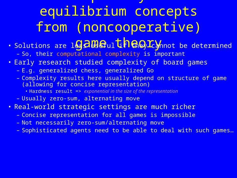
Complexity of equilibrium concepts from (noncooperative) game theory

• Solutions are less useful if they cannot be determined– So, their computational complexity is important

• Early research studied complexity of board games– E.g. generalized chess, generalized Go– Complexity results here usually depend on structure of game (allowing for concise

representation)• Hardness result => exponential in the size of the representation

– Usually zero-sum, alternating move

• Real-world strategic settings are much richer– Concise representation for all games is impossible– Not necessarily zero-sum/alternating move– Sophisticated agents need to be able to deal with such games…

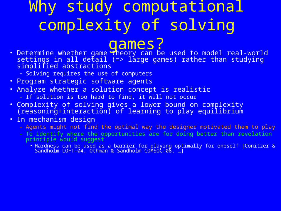
Why study computational complexity of solving games?

• Determine whether game theory can be used to model real-world settings in all detail (=> large games) rather than studying simplified abstractions– Solving requires the use of computers

• Program strategic software agents• Analyze whether a solution concept is realistic

– If solution is too hard to find, it will not occur• Complexity of solving gives a lower bound on complexity

(reasoning+interaction) of learning to play equilibrium• In mechanism design

– Agents might not find the optimal way the designer motivated them to play– To identify where the opportunities are for doing better than revelation principle would

suggest• Hardness can be used as a barrier for playing optimally for oneself [Conitzer & Sandholm LOFT-

04, Othman & Sandholm COMSOC-08, …]

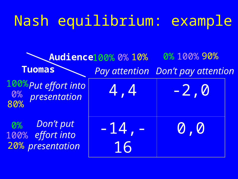
Nash equilibrium: example

4,4 -2,0

-14,-16 0,0

TuomasAudience

Pay attention Don’t pay attention

Put effort into presentation

Don’t put effort into

presentation

10%100%

0%100%

0%

0%0%

100%

100% 90%

80%

20%

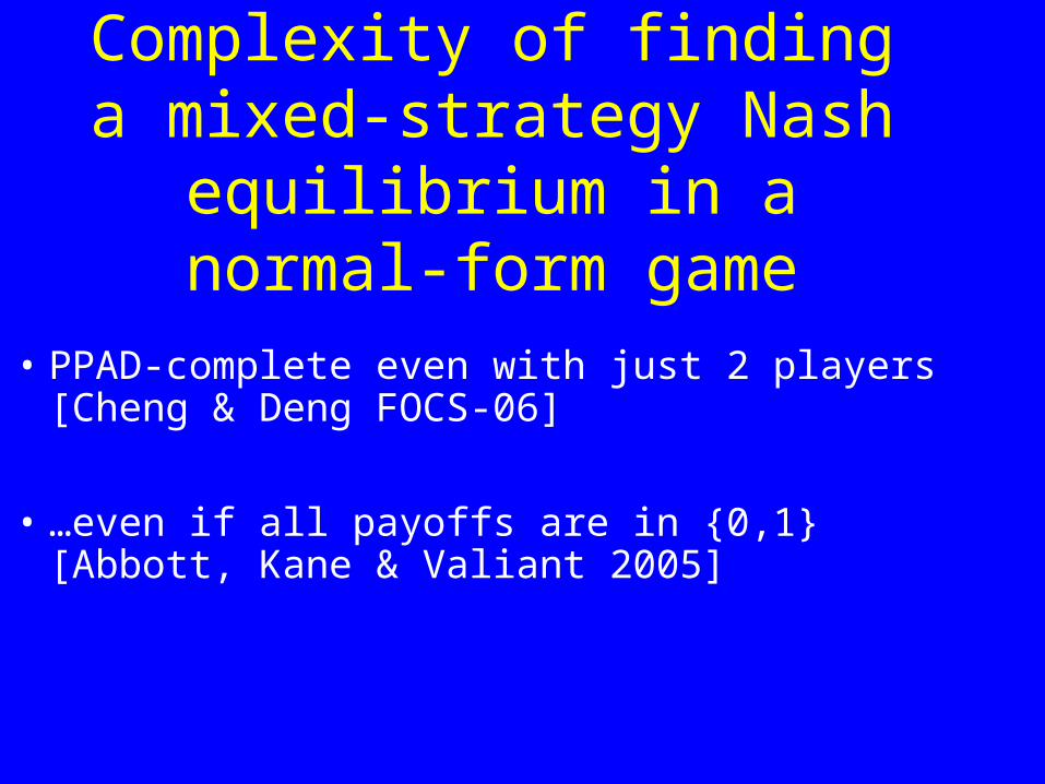
Complexity of finding a mixed-strategy Nash

equilibrium in a normal-form game

• PPAD-complete even with just 2 players [Cheng & Deng FOCS-06]

• …even if all payoffs are in {0,1} [Abbott, Kane & Valiant 2005]

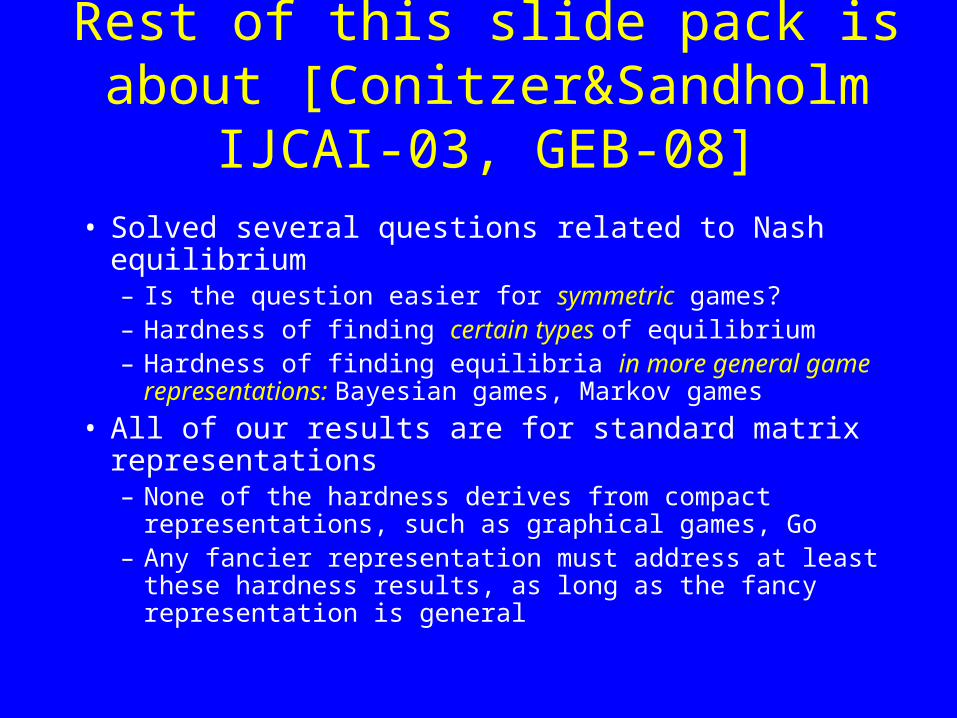
Rest of this slide pack is about [Conitzer&Sandholm IJCAI-03, GEB-08]

• Solved several questions related to Nash equilibrium– Is the question easier for symmetric games?– Hardness of finding certain types of equilibrium– Hardness of finding equilibria in more general game

representations: Bayesian games, Markov games

• All of our results are for standard matrix representations– None of the hardness derives from compact representations,

such as graphical games, Go– Any fancier representation must address at least these hardness

results, as long as the fancy representation is general

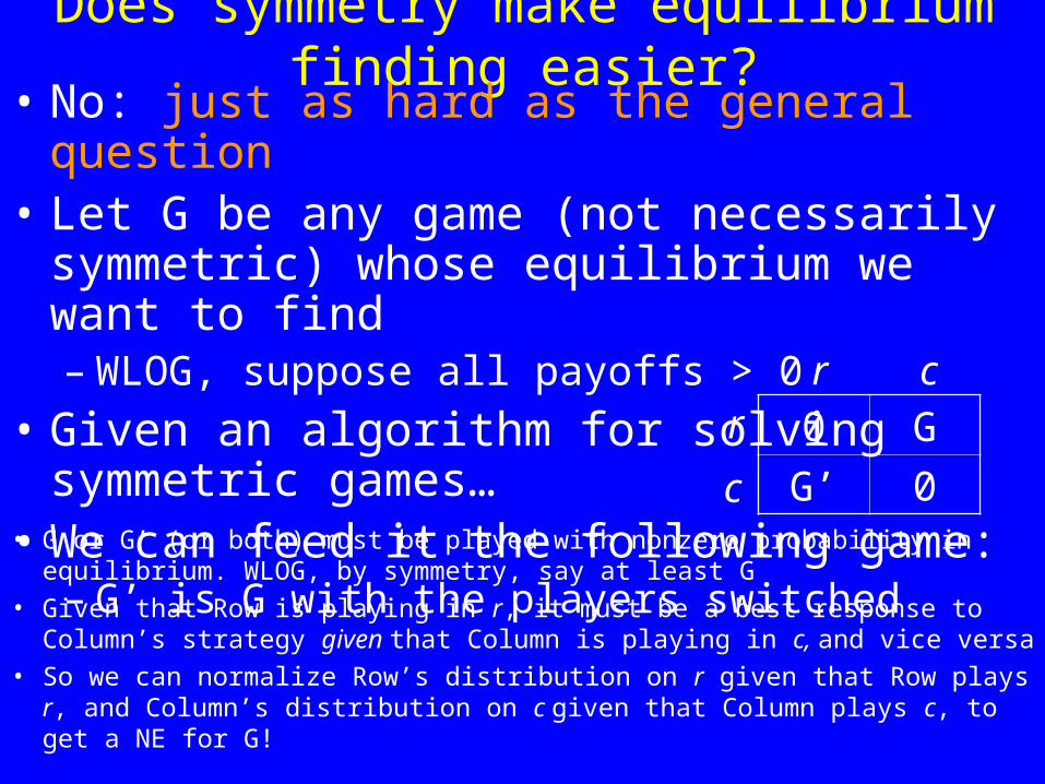
Does symmetry make equilibrium finding easier?

0 G

G’ 0• G or G’ (or both) must be played with nonzero probability in equilibrium.

WLOG, by symmetry, say at least G

• Given that Row is playing in r, it must be a best response to Column’s strategy given that Column is playing in c, and vice versa

• So we can normalize Row’s distribution on r given that Row plays r, and Column’s distribution on c given that Column plays c, to get a NE for G!

• No: just as hard as the general question• Let G be any game (not necessarily symmetric)

whose equilibrium we want to find– WLOG, suppose all payoffs > 0

• Given an algorithm for solving symmetric games…• We can feed it the following game:

– G’ is G with the players switched

crr

c

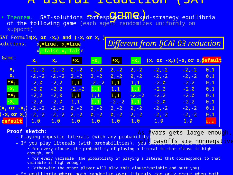
A useful reduction (SAT -> game)• Theorem. SAT-solutions correspond to mixed-strategy equilibria of

the following game (each agent randomizes uniformly on support)SAT Formula: (x1 or -x2) and (-x1 or x2 )Solutions: x1=true, x2=true

x1=false,x2=false

Game: x1 x2 +x1 -x1 +x2 -x2 (x1 or -x2) (-x1 or x2) default

x1 -2,-2 -2,-2 0,-2 0,-2 2,-2 2,-2 -2,-2 -2,-2 0,1x2 -2,-2 -2,-2 2,-2 2,-2 0,-2 0,-2 -2,-2 -2,-2 0,1

+x1 -2,0 -2,2 1,1 -2,-2 1,1 1,1 -2,0 -2,2 0,1-x1 -2,0 -2,2 -2,-2 1,1 1,1 1,1 -2,2 -2,0 0,1+x2 -2,2 -2,0 1,1 1,1 1,1 -2,-2 -2,2 -2,0 0,1-x2 -2,2 -2,0 1,1 1,1 -2,-2 1,1 -2,0 -2,2 0,1

(x1 or -x2) -2,-2 -2,-2 0,-2 2,-2 2,-2 0,-2 -2,-2 -2,-2 0,1(-x1 or x2) -2,-2 -2,-2 2,-2 0,-2 0,-2 2,-2 -2,-2 -2,-2 0,1default 1,0 1,0 1,0 1,0 1,0 1,0 1,0 1,0 ε,ε

Different from IJCAI-03 reduction

Proof sketch:– Playing opposite literals (with any probability) is unstable– If you play literals (with probabilities), you should make sure that

• for every clause, the probability of playing a literal in that clause is high enough, and • for every variable, the probability of playing a literal that corresponds to that variable is high enough• (otherwise the other player will play this clause/variable and hurt you)

– So equilibria where both randomize over literals can only occur when both randomize over same SAT solution– These are the only equilibria (in addition to the “bad” default equilibrium)

As #vars gets large enough,

all payoffs are nonnegative

Complexity of mixed-strategy Nash equilibria with certain properties

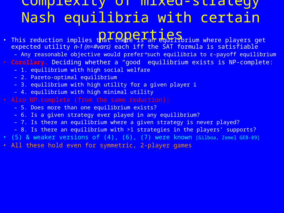
• This reduction implies that there is an equilibrium where players get expected utility n-1 (n=#vars) each iff the SAT formula is satisfiable

– Any reasonable objective would prefer such equilibria to ε-payoff equilibrium

• Corollary. Deciding whether a “good” equilibrium exists is NP-complete:– 1. equilibrium with high social welfare – 2. Pareto-optimal equilibrium– 3. equilibrium with high utility for a given player i– 4. equilibrium with high minimal utility

• Also NP-complete (from the same reduction):– 5. Does more than one equilibrium exists?– 6. Is a given strategy ever played in any equilibrium?– 7. Is there an equilibrium where a given strategy is never played?– 8. Is there an equilibrium with >1 strategies in the players’ supports?

• (5) & weaker versions of (4), (6), (7) were known [Gilboa, Zemel GEB-89]

• All these hold even for symmetric, 2-player games

More implications: coalitional deviations

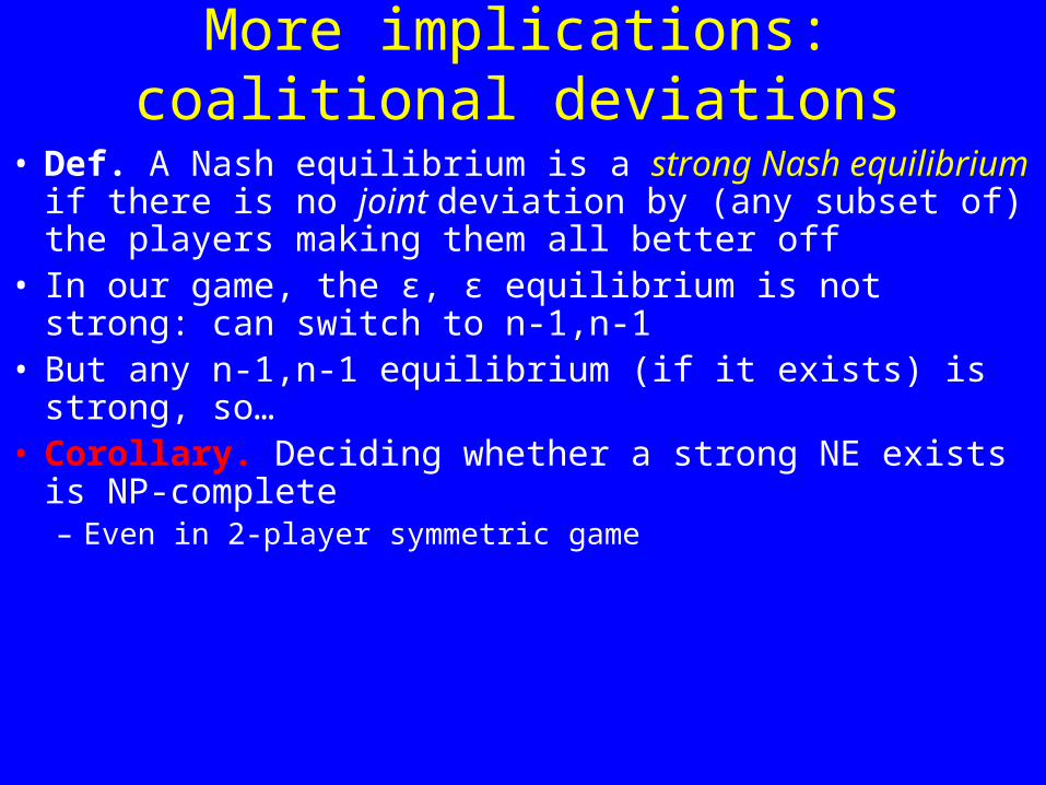
• Def. A Nash equilibrium is a strong Nash equilibrium if there is no joint deviation by (any subset of) the players making them all better off

• In our game, the ε, ε equilibrium is not strong: can switch to n-1,n-1

• But any n-1,n-1 equilibrium (if it exists) is strong, so…• Corollary. Deciding whether a strong NE exists is NP-

complete– Even in 2-player symmetric game

More implications: approximability

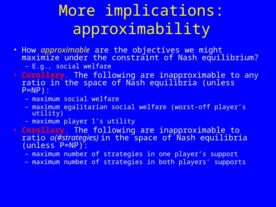
• How approximable are the objectives we might maximize under the constraint of Nash equilibrium?– E.g., social welfare

• Corollary. The following are inapproximable to any ratio in the space of Nash equilibria (unless P=NP):– maximum social welfare– maximum egalitarian social welfare (worst-off player’s utility)– maximum player 1’s utility

• Corollary. The following are inapproximable to ratio o(#strategies) in the space of Nash equilibria (unless P=NP):– maximum number of strategies in one player’s support– maximum number of strategies in both players’ supports

Counting the number of mixed-strategy Nash equilibria

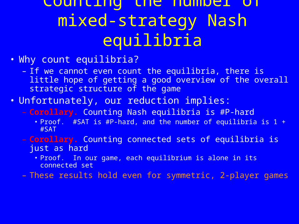
• Why count equilibria? – If we cannot even count the equilibria, there is little hope of

getting a good overview of the overall strategic structure of the game

• Unfortunately, our reduction implies:– Corollary. Counting Nash equilibria is #P-hard

• Proof. #SAT is #P-hard, and the number of equilibria is 1 + #SAT

– Corollary. Counting connected sets of equilibria is just as hard• Proof. In our game, each equilibrium is alone in its connected set

– These results hold even for symmetric, 2-player games

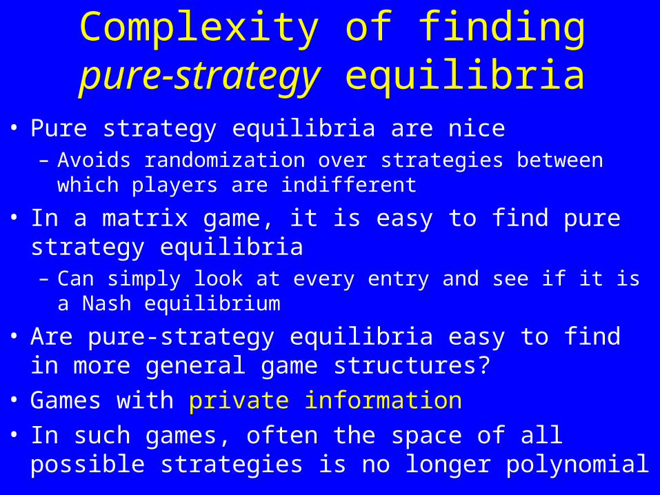
Complexity of findingpure-strategy equilibria

• Pure strategy equilibria are nice– Avoids randomization over strategies between which players are

indifferent

• In a matrix game, it is easy to find pure strategy equilibria– Can simply look at every entry and see if it is a Nash equilibrium

• Are pure-strategy equilibria easy to find in more general game structures?

• Games with private information• In such games, often the space of all possible strategies is

no longer polynomial

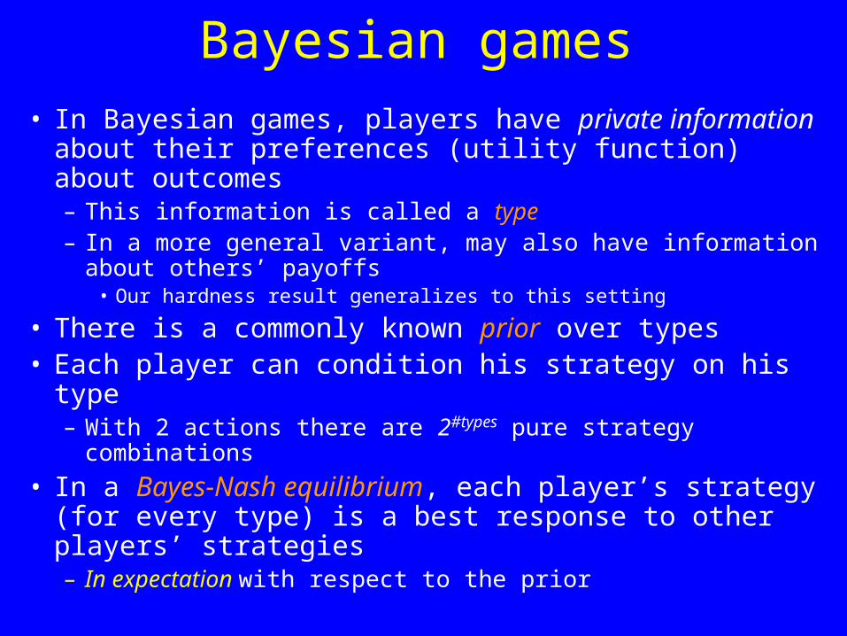
Bayesian games

• In Bayesian games, players have private information about their preferences (utility function) about outcomes– This information is called a type– In a more general variant, may also have information about

others’ payoffs• Our hardness result generalizes to this setting

• There is a commonly known prior over types• Each player can condition his strategy on his type

– With 2 actions there are 2#types pure strategy combinations

• In a Bayes-Nash equilibrium, each player’s strategy (for every type) is a best response to other players’ strategies– In expectation with respect to the prior

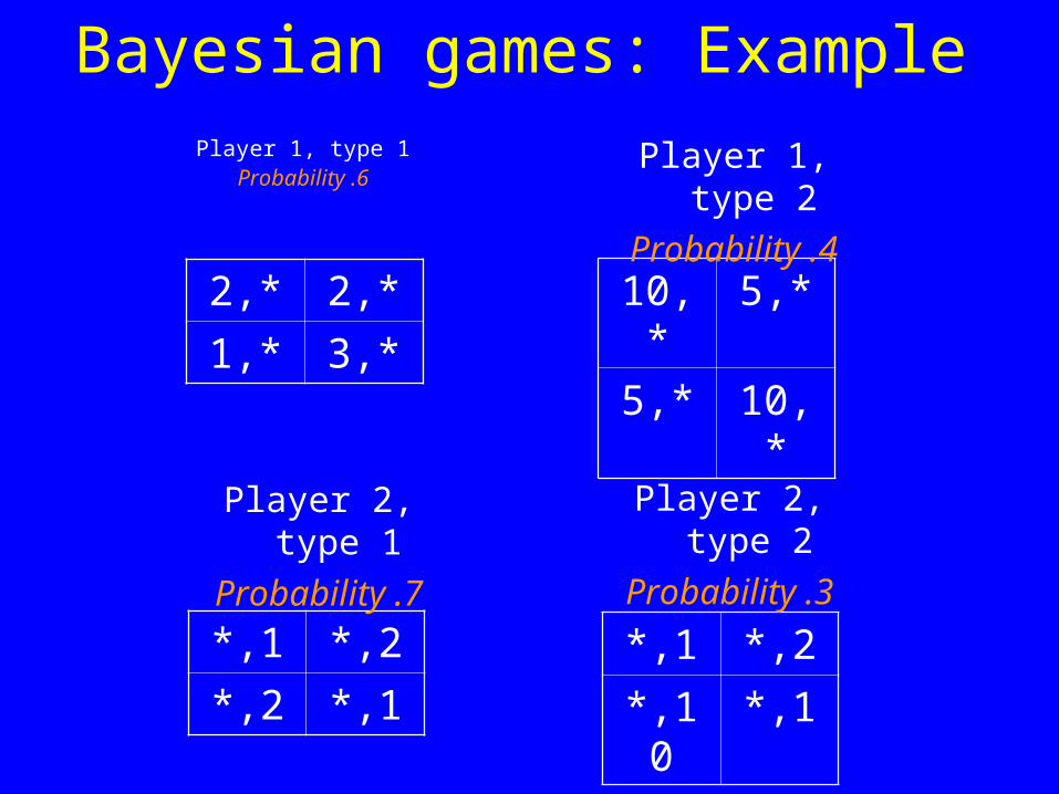
Bayesian games: Example

*,1 *,2

*,10 *,1

*,1 *,2

*,2 *,1

2,* 2,*

1,* 3,*

10,* 5,*

5,* 10,*

Player 1, type 1Probability .6

Player 1, type 2

Probability .4

Player 2, type 2

Probability .3

Player 2, type 1

Probability .7

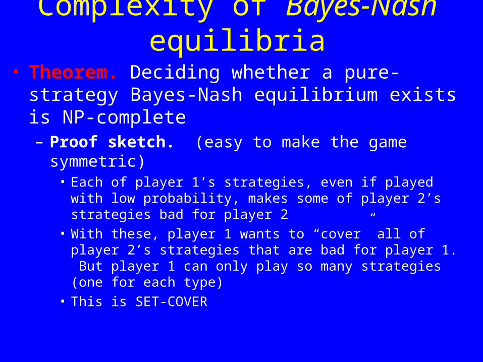
Complexity of Bayes-Nash equilibria

• Theorem. Deciding whether a pure-strategy Bayes-Nash equilibrium exists is NP-complete– Proof sketch. (easy to make the game symmetric)

• Each of player 1’s strategies, even if played with low probability, makes some of player 2’s strategies bad for player 2

• With these, player 1 wants to “cover” all of player 2’s strategies that are bad for player 1. But player 1 can only play so many strategies (one for each type)

• This is SET-COVER

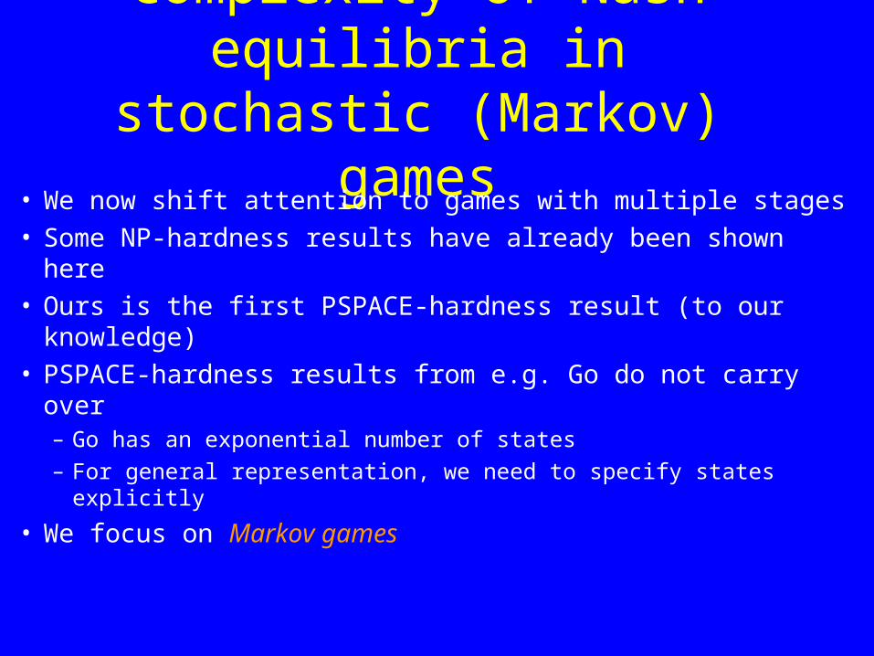
Complexity of Nash equilibria in stochastic (Markov) games

• We now shift attention to games with multiple stages• Some NP-hardness results have already been shown here• Ours is the first PSPACE-hardness result (to our

knowledge)• PSPACE-hardness results from e.g. Go do not carry over

– Go has an exponential number of states

– For general representation, we need to specify states explicitly

• We focus on Markov games

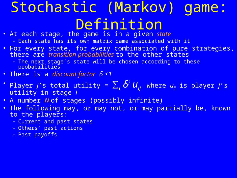
Stochastic (Markov) game: Definition• At each stage, the game is in a given state

– Each state has its own matrix game associated with it• For every state, for every combination of pure strategies, there are

transition probabilities to the other states– The next stage’s state will be chosen according to these probabilities

• There is a discount factor δ <1

• Player j’s total utility = ∑i δi uij where uij is player j’s utility in stage i• A number N of stages (possibly infinite)• The following may, or may not, or may partially be, known to the players:

– Current and past states– Others’ past actions– Past payoffs

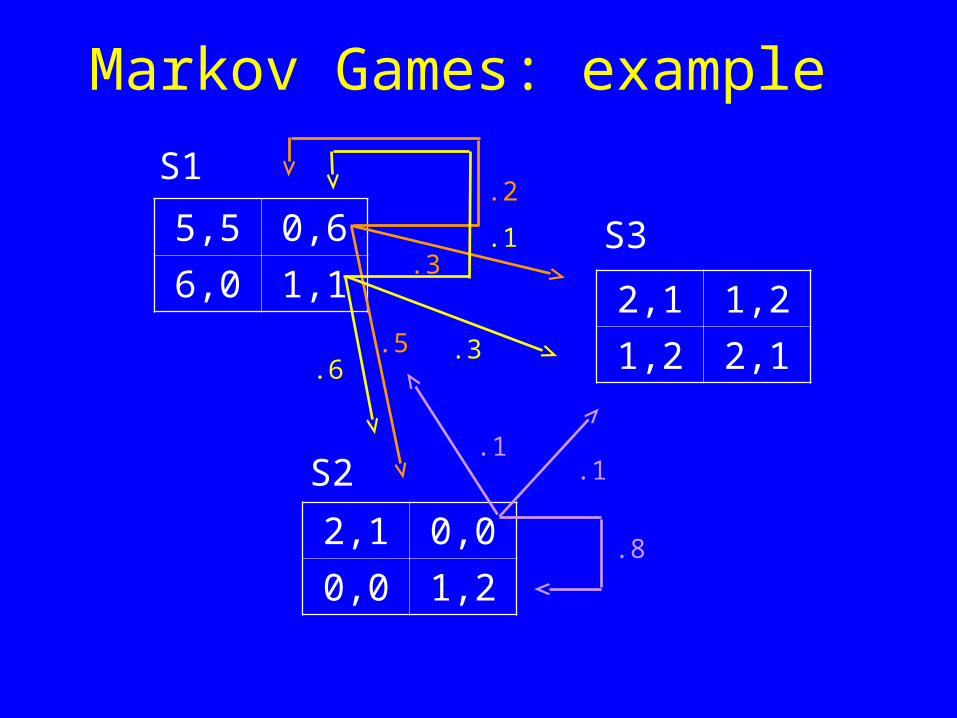
Markov Games: example

5,5 0,6

6,0 1,1

2,1 0,0

0,0 1,2

2,1 1,2

1,2 2,1

.8

.1.1

.1

.3.6

.5

.2

.3

S1

S2

S3

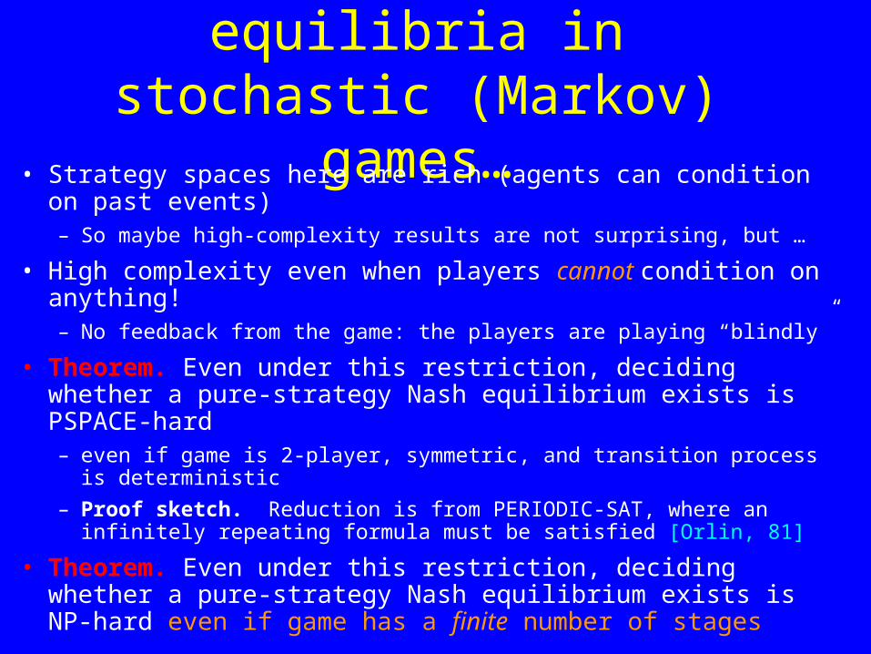
Complexity of Nash equilibria in stochastic (Markov)

games…• Strategy spaces here are rich (agents can condition on past events)

– So maybe high-complexity results are not surprising, but …

• High complexity even when players cannot condition on anything!– No feedback from the game: the players are playing “blindly”

• Theorem. Even under this restriction, deciding whether a pure-strategy Nash equilibrium exists is PSPACE-hard– even if game is 2-player, symmetric, and transition process is deterministic

– Proof sketch. Reduction is from PERIODIC-SAT, where an infinitely repeating formula must be satisfied [Orlin, 81]

• Theorem. Even under this restriction, deciding whether a pure-strategy Nash equilibrium exists is NP-hard even if game has a finite number of stages

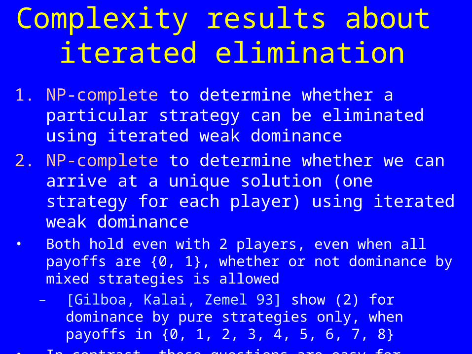
Complexity results about iterated elimination

1. NP-complete to determine whether a particular strategy can be eliminated using iterated weak dominance

2. NP-complete to determine whether we can arrive at a unique solution (one strategy for each player) using iterated weak dominance

• Both hold even with 2 players, even when all payoffs are {0, 1}, whether or not dominance by mixed strategies is allowed

– [Gilboa, Kalai, Zemel 93] show (2) for dominance by pure strategies only, when payoffs in {0, 1, 2, 3, 4, 5, 6, 7, 8}

• In contrast, these questions are easy for iterated strict dominance because of order independence (using LP to check for mixed dominance)

Thank you for your attention!