rmm

(0

OF

DECREASING NONCONFORMANCE OF PARTS

IN THE AIR FORCE SUPPLY SYSTEM

THESIS

Matthew A. StoneCaptain, USAF

AFIT/GOR/MA/88D-6

QTICSEFLECT-E

DEPARTMENT OF THE AIR FORCE

AIR UNIVERSITY C FAIR FORCE INSTITUTE OF TECHNOLOGY

Wright-Patterson Air Force Base, Ohio

jIk " -do-zcu ik" beenp

-- 'lb-f" b89 3 29 048

I°

*AFIT/GOR/KA/88D-6

DECREASING NONCONFORMANCE OF PARTS

IN THE AIR FORCE SUPPLY SYSTEM

THESIS

Matthew A. StoneCaptain, USAF

AFIT/GOR/MA/88D-6

Approved for public release; distribution unlimited

.. EIE

a

S AFIT/GOR/KA/88D-6

DECREASING NONCONFORMANCE OF PARTS

IN THE AIR FORCE SUPPLY SYSTEM

THESIS

Presented to the Faculty of the School of Engineering

of the Air Force Institute of Technology

Air University

In Partial Fulfillment of the

Requirements for the Degree of

Accession ForMaster of Science in Operations Research is .R&I---

DTIC TABUnanouwced E]Justification

Matthew A. Stone, B.S. ByDistribution/

Captain, USAF Availability Codes

'Avai' Sld-/orDiet Special

December 1988 /

Approved for public release; distribution unlimited

0 "

0z

Preface

I believe that the Air Force needs to find a logical way to lower

the nonconformance rate of its parts to an appropriate level. I use

the phase 'appropriate level' because I do not believe that the Air

Force should try to decrease nonconformity to zero; the cost to do this

would be unrealistically high. The Air Force needs a framework for

balancing the costs associated with nonconforming parts against the

costs associated with decreasing that nonconformance. I believe this

study has taken a step in the right direction to do just that.

In developing this model and writing this thesis, I have had help

from many people. My thesis advisor, Capt Joe Tatman, provided many

insights into the problem. His enthusiasm and optimism were much

needed and greatly appreciated. My appreciation is also extended to

Maj Joe Litko and Maj Ken Bauer for their advice. Their ideas helped

to make my work better. I also wish to thank my thesis sponsor, Bruce

McKalip, from the headquarters of the Air Force Logistics Command. His

assistance in helping me to better understand the problem was

invaluable. Finally, I wish to thank my wife, Santa, whose

* understanding, support, and good humor enabled me to give my best

effort on this thesis.

Matthew A. Stone

0 ii

I

8 Table of Contents

Page

Preface .......................................................... ii

List of Figures................................................... v

SAbstract........................................................ vi

I. Introduction ............................................... 1

Background ............................................ 1

Research Objective .................................... 2Benefits .............................................. 3Relationship to MIL-STD-105D .......................... 3Assumptions ........................................... 5Scope of this Study ................................... 5Decisions ............................................. 6Summary of Results .................................... 7

II. Methodology ................................................. 9

Introduction .......................................... 9Defining the Decision Maker ........................... 9Previous Analysis ..................................... 9The Problem ........................................... 11The Decision .......................................... 12

III. Model Structure ............................................. 14

A Simple Model ........................................ 15Merits of the Simple Model ............................ 20Limitations of the Simple Model ....................... 21An Expanded Model ..................................... 21Merits of the Expanded Model .......................... 23The Value Function of the Expanded Model .............. 25Assumptions of the Expanded Model ..................... 26

* Limitations of the Expanded Model ..................... 26

IV. Applying Response Surface Methodology to PerformSensitivity Analysis on a Decision Analysis Problem ......... 28

Inputs to the Model ................................... 29Outputs from the Model ................................ 30Design of the Experiments ............................. 31

First Design ..................................... 31Results from the First Design .................... 33Second Design .................................... 34Results from the Second Design ................... 35

* Conclusions from the Sensitivity Analysis ............. 41

iii

V. R s l s. ..........................4

V.apl Rsls................................................. 43

Exarple.........e....a.. ep..........................46Forcing GA to be 0 (accept) ....................... 46

'SVI. Conclusions................................................. 55

Lack of Real Data ..................................... 55Uses of the Model ................................... 5Procedure vs. Results ...... ........................... 57Necessary Improvements ................................ 58

Ap;endix A: Output from the Runs Used forSensitivity Analysis ................................. 60

Appendix B: Variable Settings and Output Values ................... 61

Bibliography...................................................... 62

Vita ............................................................. 63

iv

List of Figures

Figure Page

1. Influence Diagram of the Simple Model ........................ 16

2. Discretizing a Continuous Probability Distribution ........... 18

3. Influence Diagram of the More Complex Model .................. 24

4. Residual Plot for the Second Design .......................... 37

5. Response Surface Used for the Sensitivity Analysis ........... 39

6. Influence Diagram When the Government Action (GA)Decision Is Always Forced to 0 (Accept) ...................... 44

7. Influence Diagram When the Government Action (GA)Decision Is Always Forced to 1 (Reject) ...................... 45

8. Response Surface When GA Decision Is Forced to 0 ............. 48

9. Response Surface When GA Decision Is Forced to 1 ............. 50

10. Intersection of the Two Response Surfaces .................... 51

11. Line Where the Two Response Surfaces are Equal ............... 52

AFIT/GOR/MA/88D-6Abstract

The purpose of this study was to provide AFLC (Air Force Logistics

Command) with a prototype decision model which will help AFLC engineers

decide when post-production testing for a particular NSN (National

Stock Number) is beneficial to the Air Force, as well as what action

the Air Force should take as a result of that testing. The problem is

a two sided issue. On one hand, nonconformance costs the Air Force in

terms of damaged equipment and potential harm to personnel. On the

other hand, the Air Force cannot afford to test everything. The study

provides an initial step in developing a decision aid to help AFLC

allocate its scarce testing resources.

Sensitivity analysis was performed on this model by using the

techniques of Response Surface Methodology. For the data used in this

study, the random variable which has the greatest impact on the ex-

pected cost to the Air Force is the expected dollar value that a single

part can be expected to cause given that the part is in nonconformance

with its specifications. This result was confirmed using traditional

EVPI (expected value of perfect information) calculations.

The most significant contribution of this study is the development

of a graphic decision aid. With this aid, the decision maker can

graphically see how the present situation relates to a 'break-even

line', or indifference curve. In addition to showing the decision

maker which alternative is optimal, this method shows how much the

independent variables would have to change for the optimal alternative

to change.

vi

U

DECREASING NONCONFORMANCE OF PARTSIN THE AIR FORCE SUPPLY SYSTEM

I. Introduction

Background

The Air Force Logistics Command spends $13 billion a year

procuring products for its supply system (5). The total Air Forcc

budget for FY 88 excluding military pay and retirement is over $62

billion (2:C-4). Therefore, over twenty percent of the Air Force

budget is spent every year just to replenish its supply inventory. The

Air Force supply system is so large that even a small percentage of

nonconformity in the inventory can have a major impact on the Air Force

budget. When nonconformance in present, money that could have gone to

other Air Force missions must be used to replace parts that do not work

or last as long as they should have. In either case, when

nonconformance exists, the Air Force is not getting what it's paying

for.

The government goes to great lengths to ensure that the parts

procured for use in all military equipment are able to perform the

mission reliably. Military contract specifications are written,

government inspectors are stationed in contractor factories through the

DCAS (Defense Contract Admini.stration Service) system, and first

article testing is performed, Ili in an effort to try to prevent poor

quality parts and mP-erial fror antering the supply s,.Lem of the

1

0

military services. However, as one might expect, a certain proportion

of these parts and supplies do not meet the military specification for

their manufacture and performance. When a part fails to meet its

specification, the consequences are often minor, but sometimes, such a

failure results in a major weapons system failure. Being the manager

of the Air Force supply system, the Air Force Logistics Command (AFLC)

is understandably concerned about the problem of nonconforming parts

and material. A preliminary report of some nonconformance testing

performed at Warner Robins ALC in 1986 and 1987 indicates that a

significant number of parts in their inventory do not conform to

contract specifications. The report recommends that post-production

testing (the testing of items after they are already in the inventory)

be performed on all Federal Stock Classes (FSCs) which are important

and which have demonstrated high nonconformance in the part.

Obviously, AFLC does not have the resources to test all of its

Federal Supply Classes. Furthermore, it may not be economically sound

to try to do testing on all FSCs. The purpose of this thesis is to

provide a prototype tool which will assist AFLC in decidii, h I(w much

testing should be done on any given Federal Supply Class (FSC) or

National Stock Number (NSN).

Research Objective

The objective of this research is to provide a prototype decision

* tool to AFLC engineers to help them make the following decisions:

1. When is post-production testing of a particular NSN economically

wise?

2

2. Once AFLC engineers decide which NSNs to test, how many items in

each NSN should be tested?

3. Based on the results of the post production testing for a

particular weapon system, what actions should AFLC take to insure the

operational safety of the weapon system?

Benefits

The benefits to be gained from this sort of post production

testing are numerous. The first benefit is short-term in that we can

identify and eliminate nonconforming parts from the inventory today.

The second benefit is the creation of a database which would provide an

indication of how well products from different contractors conform to

specifications. The third benefit is more long-term. Just the

existence of a testing program in itself and a database of contractor

performance could raise the quality of parts that are received from the

private industry. The testing results could help to provide an

objective way for the Air Force to prevent poor quality manufacturers

from winning government contracts. These actions would alert the

defense manufacturing community of a new tougher stance by the Air

Force and should be expected to increase overall quality in the long

run.

Relationship to MIL-STD-105D

Military Standard 105D is a widely accepted tool which contains

many detailed tables and charts useful for acceptance testing. Tt is

used when the military is going to test an NSN and either accept or

reject a lot of that NSN based on the outcome of that testing. If one

3

knows the population size and the Acceptable Quality Level (AQL), one

can determine from Mil-Std-105D how many units should be tested from

that NSN and how many have to be good in order to accept the lot.

The drawback to using Military Standard 105D is that the numbers

it provides were derived in isolation from the specific problem at

hand. When Mil-Std-105D says that X units need to be sampled in order

to be 90 percent sure that we have achieved the minimum accepted

quality level, it does not consider the costs involved with testing,

the costs associated with rejecting the lot, or the cost of having

nonconforming parts in the inventory which may eventually cause

significant damage to a weapons system and/or crew. Or, it may be that

testing the number of units recommended by Mil-Std-105D may simply be

too expensive due to large set-up costs, limited testing resources, a

large manpower requirement to perform the testing, or any combination

of these factors.

A pure statistician may find these costs to be annoyances which

muddy the water. However, a good decision maker wi)l either

consciously or subconsciously take all of these costs into account.

Therefore, a good model of the decision problem must also try to model

all of these costs. The complication is that almost all of these costs

are very uncertain and therefore difficult to quantify. No real data

exists for these unknown costs, however, there may exist experts who

can provide their subjective inputs as to what these costs might be.

Decision analysis provides a methodology for quantifying the subjective

opinions of experts and including them in the analysis. This thesis

uses decision analysis methods to try to do just that.

4

This thesis is not trying to suggest a way to replace Mil-Std-

105D, -nly a way to supplement it. Whereas Mil-Std-105D sees the

accept or reject question from a purely statistical point of view, the

model presented in this thesis tries to account for the real world

subjectivity that truly affects the decision. The mathematics of Mil-

Std-105D are clean and precise yet too simplistic. The model in this

thesis may be called fuzzy because it contains much subjective data yet

therein lies its strength in that it attacks the decision from a

holistic point of view. In addition to Mil-Std-105D, the model in this

thesis can help the decision maker make a better decision of how many

items to test.

Assumptions

The assumption of this thesis is that AFLC has subjective

knowledge about which NSNs or FSCs have a problem with nonconformance.

There are several ways in which this subjective information could be

quantified. The number of Quality Deficiency Reports (QDRs) or

Material Deficiency Reports (MDRs) issued on an item could be a good

indication that a problem with nonconformity exists. Another

indication of a problem with nonconformance could also be provided by

the engineers at the ALC where the item is managed. Once subjective

information is gained that a problem with nonconformance exists, the

decision tool of this thesis should be applied to determine what

a(.ions should be taken.

Scope of this Study

This thesis effort is designed to provide a prototype model of the

5

decision process just described. Although the model correctly captures

the essence of the problem, the alternatives for the two decisions need

to be expanded and made more realistic. Currently the alternatives for

NTEST (the number of items to test) are limited to three items tested,

and the alternatives for GA (government action) are limited to accept

and reject.

To be truly beneficial to the end user, a user friendly "front

end" must be added to this model, as well as graphical outputs that are

meaningful to the user.

Decisions

There are two main decisions facing the decision maker. The first

decision is how many units to sample and test for conformance to

specifications. In the formulation of the problem that follows, this

first decision is referred to as NTEST. The second decision is what

action the government (specifically the Air Force) should take. This

second decision is made in light of the results of any testing that is

performed. This second decision is referred to as GA. The goal of

using this model is to provide the decision maker with the optimal

alternatives for both of these decisions which minimize the expected

* cost to the Air Force.

The alternatives for the second decision, GA, are 0 and 1. If GA

is set to 0, it implies no action taken by the Air Force. If GA is set

* to 1, it implies action taken by the Air Force. It may seem that

limiting the alternatives of GA to only two values is not a realistic

representation of all the alternatives that are truly available to the

* Air Force in this situation. However, this seeming lack of realism is

6

compensated for by using a variable to represent the cost of the Air

Force's action, COSTGA. The actual value of the cost of the Air

Force's action varies depending upon the probability distribution that

defines it. This probability distribution is provided by the user.

Therefore, instead of having only two alternatives for the Air Force's

action, this problem can represent a whole range of actions which are

identified by their cost. Each different value for the cost of the Air

Force's action (COSTGA) represents a different alternative for the Air

Force's action (GA).

Summary of Results

This study provides AFLC with a prototype decision model which can

be adapted to any particular NSN which is thought to have a

nonconformance problem. This prototype decision model is designed to

help AFLC decision makers decide when post-production testing is

beneficial to the Air Force, as well as what action the Air Force

should take as a result of that testing. The use of this tool will

give AFLC insight about how to spend its scarce testing resources. It

will also provide a logical way to start gathering an historical

database of contractor performance in the production of specific items.

A new type of sensitivity analysis is used on the model in this

thesis. The techniques of Response Surface Methodology (RSM) are used

to determine which random variable has the greatest impact on the

response variable, expected cost to the Air Force. For the data used

in the example, the response variable is most sensitive to changes in

the variable DAMGBP (Damage Given the Part is Bad). The results of the

7

sensitivity analysis are also confirmed by traditional EVPI (Expected

Value of Perfect Information) calculations.

The most significant contribution of this thesis is the

development of the methodology used in chapter V. Figure 11 is an

example of the kind of graphic decision aid which can be produced with

this methodology. A graph, such as the one in Figure 11, has two major

features which make it extremely useful to the decision maker.

The first feature is the fact that two of the independent

variables are varied over a wide range. This feature allows the

decision maker to use a wide range of values for some unknown random

variable instead of having to restrict the analysis to a more precise

estimate of the unknown random variable.

The second feature is that the decision maker can graphically see

how the present situation relates to the so-called 'break-even line'

Instead of just telling the decision maker which alternative is

optimal, this method shows the decision maker how much the independent

variables would have to change for the optimal alternative to change.

8

II. Methodoloay

Introduction

During the course of this study, much time and effort was spent

just trying to define the problem. There are many competing political

interests as well as many technical aspects to this problem. IL order

to better understand all the issues surrounding the problem, the author

spent much time learning about how the Air Force manages its material

inventory. This investigation focused on who is involved in managing

any particular item and who the actual end user of a decision support

tool would be. The author also examined the preliminary results of the

study being conducted by the Inspector General of the Department of the

Air Force (DoD/IG).

Defining the Decision Maker

Within AFLC, the activity of managing supply items is performed by

many specialized career fields. Item managers, equipment specialists,

engineers, primary contracting officers, and administrative contracting

officers are all involved at some point in the process. When an item

is believed to have problems with nonconformance to specifications

however, it is the engineers who are primarily responsible for

rectifying the problem. Therefore, the engineers were targeted as the

decision makers in this problem and the decision tool was tailored for

their use.

Previous Analysis

The next step was to learn more about the DoD/IG's investigation

9

of nonconforming parts in the Air Force. In 1986, the Inspector

General of the Department of Defense (DoD/IG) began a program to

determine the extent that products in the DoD were in nonconformance to

the specifications for their manufacture and performance. The first

stop in their audit was Warner-Robins Air Logistics Center (WR-ALC) in

Georgia. Because of a cutback in funding, the DoD/IG was forced to

scale back the number of items to be tested as well as the number of

Federal Supply Classes from which the items would be sampled. The

preliminary findings of DoD/IG's audit report indicates that a very

significant percentage of parts in the Warner-Robins AFB inventory are

in nonconformance of their specifications. As a result of the cutback

and subsequent small sample sizes, AFLC is concerned about the accuracy

of the DoD/IG's sampling techniques and the validity of the inferences

that will be drawn from the sampling.

If the DoD/IG made correct use of sampling during their audit,

they would be able to observe a small portion of some population and

draw inferences about the population as a whole. Of course, the

validity of their inferences depends greatly on how representative

their sample was of the entire population.

In order to learn more about how the DoD/IG collected their

sample, this author contacted the project officer of the DoD/IG audit

as well as the statistician who designed the sampling strategy used

during the audit. Neither one was able to provide any details about

the sampling strategy.

For lack of better knowledge, this author assumed that the audit

used some type of attributes sampling plan. An attributes sampling

10

0

plan is a sampling plan where a particular attribute of an item is

tested and the only information recorded is whether or not the item

tested conforms to some specification (3:63). A single attribute

sampling acceptance plan (SASAP) is designed to provide a consumer with

a desired level of protection against accepting a lot in which the

proportion of defectives associated with a certain attribute exceeds an

acceptable level. Military Standard 105D (Mil-Std-105D) contains

extensive tables useful for designing an attributes sampling plan.

The audit is also believed to have used quota sampling as opposed

to full probability sampling. Quota sampling is a type of sampling

where the number to be sampled from each stratum is decided in advance

and the experimenter continues to sample items until the necessary

quota is obtained in each stratum (1:105). Quota sampling is preferred

by some survey researchers because it is easier and more inexpensive to

implement than full probability sampling. Cochran describes quota

sampling as "stratified sampling with a more or less nonrandom

* selection of units within strata" (4:890). According to Benjamin King,

the most important shortcoming of quota sampling, and nonprobability

sampling in general, is the inability to calculate the mean square

estimation error (4:890). The mean square estimation error cannot be

determined due to the inherent selection bias of quota sampling.

Without knowing the mean square estimation error, there is no way of

knowing how accurate the estimate really is.

The Problem

In response to the preliminary findings of the DoD/IG's audit

11

report, the Air Force Logistics Command (AFLC) coild decide to

institute a post-production testing progan that will test all critical

parts to insure that they conform to their specifications. AFLC does

not have the testing resources to test every single part that it

manages, therefore, AFLC must decide which National Stock Numbers

(NSNs) should come under the testing plan if one is implemented. The

Air Force cannot afford to test its entire inventory, however, the Air

Force also cannot afford to have parts in its inventory that are in

significant nonconformance to specifications and could possibly cause

major malfunctions. Therefore, the challenge is to tind a logical way

to balance the risk associated with nonconforming parts against the

cost of testing them.

The Decision

The decision analysis methodology is used to structure the problem

and to aid AFLC decision makers in understanding the problem. There

are two decisions which are modeled. The first decision is how many

units to sample and test for conformance to the specifications. The

second decision is what action the Air Force should take in light of

the testing that is performed. The outcome of the model iL the

expected total cost to the Air Force. In decision analysis terms,

expected total cost to the Air Force is the value node, and the

objective is to minimize this cost. The expected total cost to the Air

Force is comprised of three costs considered in this model: the

testing costs; the costs associated with nonconforming parts; and, the

costs for the Air Force to take some type of action to correct the

problem.

12

The author assigned the ranges and the probability distributions

associated with each unknown cost. The emphasis was on developing a

model that is structurally correct. The true ranges and probability

distributions of each cost need to be obtained to reflect the true

knowledge from the decision makers who will actually use this model

when it is expanded from a pilot model into a full-scale model.

The initial model was analyzed using a decision analysis software

program called Performa. Deterministic sensitivity analysis was

performed. The model was then expanded and analyzed using another

decision analysis program called InDia. A different type of

sensitivity analysis using response surface methodology was then

conducted on the expanded model. The results of the sensitivity

analysis provide a measure of the importance of quantifying the unknown

probability distributions. More time and effort should be spent on

getting an accurate probability distribution on those variables to

which the response is most sensitive. Finally, regression techniques

are used to show how the optimal alternative for the GA decision

(whether or not the Air Force should take action) changes as the

unknown independent variables change. By doing so, it allows the

decision maker to graphically see how changes in the independent

variables can affect the decision of whether or not the Air Force

should take action.

13

III. Model Structure

The model of this decision process is represented with an

influence diagram. Influence diagrams provide a convenient way of

representing a decision analysis problem more compactly than using a

conventional decision tree. An influence diagram is a way of

representing a decision process with nodes and arcs. Different nodes

represent different types of variables which can be decisions, random

variables, deterministic functions or value nodes. The arcs between

the nodes represent dependencies of one node upon another. Once the

influence diagram is built, the influence diagram can be reduced and

solved to provide the optimal decision alternative and the expected

value of that optimal decision alternative. Several other analyses are

available to the decision analyst to gain a better understanding of the

problem.

The three main costs that are considered in both models are: the

testing costs; the costs associated with nonconforming parts; and the

cost for the Air Force to take some type of action to correct the

problem.

The testing costs are structured to account for fixed testing

costs and variable testing costs. Fixed testing costs include special

testing equipment and tools and any other start-up costs. Variable

testing costs include the manpower to perform the testing and the cost

of the actual unit that is sampled if the testing is destructive.

The costs of nonconformance are incurred when parts are in

* nonconformance to their specifications yet they remain in the inventory

14

and have the potential to cause damage. The costs due to

• nonconformance include the cost of the defective unit, the cost to buy

another unit to replace it, and the cost of higher assemblies that may

be damaged due to failure of the nonconforming part. The decision

* maker must base his decision on the relationship between all of these

costs. The decision maker must weigh the costs of an extensive testing

program against the risks and costs associated with high nonconformance

* of parts in the inventory.

The following constants are used throughout each run of the model.

The user of the model can change any constant before each run, however,

* its value will not vary during the run.

1. Fixed testin costs

2. Variable testing costs

* 3. The total number of units in the population

4. The maximum number of units that can be sampled from the population

A Simple Model

The first attempt at formulating a model of this decision process

focuses on what appears to be the main decision which is to determine

the number of units that should be sampled for a particular NSN that is

suspected to have a nonconformance problem. This decision is labeled

as NTEST in the influence diagram which is shown as Figure 1. The goal

of using this simple model is to provide the decision maker with the

optimal alternative for NTEST which minimizes the expected cost to the

Air Force. The alternatives for NTEST can theoretically be anything

from zero up to N, the total number of units in the NSN. If XTEST is

15

LA.

*N N

=CL

166

Sr

zero, it implies that no testing for conformance to specifications is

performed. If NTEST is N, it implies 100 per cent testing for

conformance to specifications. For the sake of simplicity, NTEST is

artificially limited to range from 0 to 3 in the simple example.

TPG (True Percent Good) is the true percentage of units in the

inventory of this type that meet the desired specification. For

example, if tne mean of the values for TPG is 0.8, then we can expect

that 8 out of 10 units conform to specifications. It is important to

note that in this model TPG is not just one number; it is a cintinuous

random variable. The same is true for all the single circle nodes

(also called chance nodes) in the influence diagram. Before the

problem can be solved, however, all of the continuous random variables

must be discretized. The author assumed that all of the random

variables were approximately normally distributed. See Figure 2 for an

example of how the variable TPG is discretized. Notice in Figure 2

that TPG is discretized to three possible values where 0.73625 is the

mean of the lower quartile, 0.80 is the mean of the two middle

quartiles, and 0.86375 is the mean of the upper quartile.

The nodes Xl, X2, X3 represent the first, second, and third units

that are sampled from the NSN. For this simple problem, a maximum of

three units can be tested. The outcome for Xl, X2, and X3 is one if

the item conforms to specification, and zero if the item does not

conform. The probability of whether Xl, X2, or X3 is a one is

dependent on the mean value used for TPG (true percentage of units in

the inventory that conform). For example, if a mean value of 0.8 is

used for TPG, then there is an 80 percent chance that Xl will be one.

17

0

.0

.0CL

6(00

c4-

ou-~ .0

6Z

C; Chco CN0

* L.

A1111Y900.

18,

NUMGOOD is a deterministic function that merely sums the results

of testing sample units Xl, X2, and X3. It could happen that no units

are sampled, and in that case, NUMGOOD would be zero.

In Figure 1, there is only one decision node present, NTEST.

NTEST is a decision node for how many units should be tested. The

input for NTEST is all the possible alternatives for the number of

units -o be tested. The optimal number of units to test is obtained by

solving the influence diagram. In this small example, the decision

alternatives for NTEST range from zero to three units that can be

tested.

FLAG is only used to signal to the value function whether at least

one unit has been tested.

The value node in this influence diagram is the cost to the Air

Force. The function which represents the Air Force's cost is:

FLAG*[-1000.0-240.0*NTEST-EXP(ABS((TPG*NTEST)-NUMGOOD))+I.O]

where FLAG is a binary variable indicating whether any testing was

done, NTEST is the number of units that are sampled, TPG is the true

percentage of units that conform, and, NUMGOOD is the number of units

that conform among those sampled.

In this function, FLAG is 1.0 if NTEST is greater than or equal to

one. The fixed testing costs include special testing equipment and any

other costs to start a new testing program of this sort. In this small

example, the fixed testing costs are set at $1000.00. The variable

testing costs include the manpower to perform the testing and the cost

of the unit itself if the testing is destructive. The variable testing

19

0

costs are set at $240.00 per unit tested. The remainder of the value

function is based on the idea that there is a cost associated with not

knowing the true value of TPG. In other words, a cost is incurred

which is proportional to the error in the estimate of TPG. The Air

Force places a high value on knowing the true value of TPG (the true

proportion of units that meet the specification). The value function

above incurs a smaller cost (greater value) when TPG*NTEST is closer to

NUMGOOD. Conversely, the Air Force has a lower value for when TPG and

NUMGOOD are farther apart. The reasoning behind this value function is

that the Air Force can make better decisions about the management of

this particular NSN if the Air Force knows the true percentage of units

that conform to the specifications. A better estimate of this true

percentage is obtained when more testing is done, therefore, in this

small example, the optimal alternative for the number of units to test

is always the highest number of units, three in this case. If the

alternatives for NTEST were allowed to be sufficiently larger, then

there may come a point when the additional testing costs do not warrant

the gain in information that results from that testing. At that point,

the optimal alternative for NTEST would not be the highest alternative.

Merits of the Simple Model

The advantage of the simple model in Figure 1 is that it is a

representation of the decision process which focuses on the main

decision which is the number to sample (NTEST). The advantage of this

representation is that it focuses on the decision maker's real

interest, the number of items that should be tested. The simpler model

0 is also easier to understand. However, by using this simpler model,

20

realism is sacrificed.

Limitations of the Simple Model

The disadvantage of the simple model in Figure 1 is that the value

function is extremely arbitrary. The value function assumes that the

Air Force always has more value when the estimate for the percentage

that conform (NUMGOOD/NTEST) is closer to the true percentage that

conform (TPG). This may in fact be the case, but it is doubtful that

the value of that difference is truly represented by an exponential

function. In any case, the model is vague about the value of having

TPG close to (NUMGOOD/NTEST).

Another disadvantage of the simple model in Figure 1 is its

nearsightedness. It does not consider what decisions will be made

later as a result of the testing that is done now. As a result, it is

impossible to calculate an accurate value of information on the random

variables because changes in the random variables do not impact

decisions that will be made in the future.

To develop a better value function, it's necessary to know what

decisions will be based on the results of the testing. To properly put

a value on that testing, it's imperative to know how the results of the

testing affect future decisions.

An Expanded Model

In addition to the decision of how many units to test (NTEST),

there are at least two more decisions that are relevant to this

nonconformance problem: an operational decision; and a financial

decision.

21

The operational decision focuses on what actions the Air Force

should take to improve the present quality of the spare parts that are

supporting the flying mission. The operational decision is mainly

dependent on the results of any testing that is done. The operational

decision encompasses the risks associated with using the parts against

the cost of taking actions to improve the situation. We can try to

estimate the risks associated with using the present inventory of parts

and find the point where the risk is balanced by the cost of taking

action to correct the problem. The point where these two costs are

balanced can be graphed for a differing number of sample sizes and the

resultant graph will be split into two regions. In one region, the

optimal decision would be to accept the parts and follow the status

quo. In the other region, the optimal decision would be to reject the

parts and take some type of action to correct the problem such as

procuring new parts (preferably from a higher quality source). By

presenting the problem in the appropriate way, the decision maker's

task is reduced to making a judgment about whether the true value of P

is greater than or less than some value. This should be an easier task

than trying to determine the prior probability distribution on P. In

any case, the additional information should be helpful' See chapter V

for a further explanation of this use of the model.

The financial decision focuses on what actions the Air Force

should take concerning the contract and the manufacturer. The

financial decision depends on many other outside factors in addition to

the testing results and the operational decision. When making the

financial decision, the Air Force must consider the past performance of

22

the manufacturer, the size of the contract, the seriousness of the

nonconformance, the willingness of the manufacturer to correct the

defect, and the probability that any legal action taken will be

favorable to the Air Force.

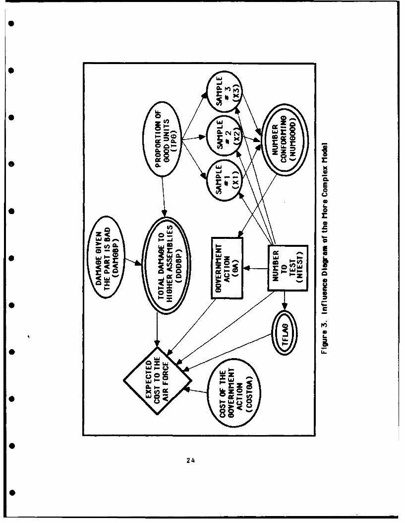
Merits of the Expanded Model

The expanded model in Figure 3 is only concerned with the

operational decision. It attempts to correct some of the deficiencies

of the simple model in Figure 1. The main difference between the two

models is the inclusion of a second decision node, Government Action

(GA), which represents the operational decision that must be made. By

adding the GA node, the model in Figure 3 is a better representation of

the decision process because it models how the results of the testing

affect the future decision, GA. The alternatives for the GA decision

node are 0 and 1 where 0 represents no action taken by the government

and 1 represents action by the government. This action taken by the

government is not specifically defined. The action could be freezing

the entire stock of the item until 100% inspection is made, purging the

stock and procuring new stock from a different manufacturer, or any

other action the government believes appropriate.

Another addition to the influence diagram in Figure 3 is the

addition of the chance node DAMGBP. DAMGBP (DAMage Given it's a Bad

Part) represents the expected dollar value of the damage that a single

nonconforming unit will cause.

The deterministic node DDDBP represents the expected dollar value

of the total damage that will result due to all the nonconforming parts

23

Sr

r~rx

126E

S

* a

r

z4c 4

u*4,.'Uzj w

r 01% 0 p

0- 0 u24 -P- -

in the inventory. Costs included in DDDBP are the cost of lost use of

the part and also the cost of damage done to higher assemblies. The

function for DDDBP is:

DAMGBP * (1 - TPG) * N

0

where DAMGBP is the expected dollar value of the damage that a single

nonconforming unit will cause, (1-TPG) is the percentage of parts that

do not conform to specifications, and N is the total number of units in

the NSN.

COSTGA (COST of the Government's Action) is a chance node that

contains the probability distribution on how much it will cost the

government to take some form of action.

The Value Function of the Expanded Model

0 The value node, Expected Cost to the Air Force, evaluates all of

the costs that are incurred for each possible alternative and outcome

in the influence diagram. The costs that are considered are the fixed

0 testing costs, the variable testing costs, the costs associated with a

part that is nonconforming yet remains in the inventory, and the cost

for the government to take some type of action to correct the problem.

0 The value function for the value node in Figure 3 is:

(FLAG * (-1000.0 - 240.0 * NTEST)] - [GA * COSTGA] - [(1 - GA) * DDDBP]

0 The first half of this value function adds in the fixed and variable

testing costs if any testing is done. The second half of the function

adds in the cost of government action if GA is 1, or it adds in the

0 costs due to nonconforming parts if GA is 0. The costs due to

25

nonconforming parts include the cost of the defective units, the cost

to buy other units to replace them, and the cost of higher assemblies

that may be damaged.

Assumptions of the Expanded Model

This model is not intended to be used on every NSN that the Air

Force manages Because of the time involved to input the required

information, it would be unrealistic to go through this procedure for

every NSN. This model should only be used for those NSNs which are

suspected to have a nonconformance problem.

Limitations of the Expanded Model

The model in Figure 3, while better than the model in Figure 1,

still makes some large generalizations. Specifically, many unknowns

are aggregated into one probability distribution. The chance nodes

DAMGBP and COSTGA make use of this aggregation to simplify the problem.

The two chance nodes DAMGBP and COSTGA each contain many parts.

The chance node DAMGBP (dollar value of the damage that a single

nonconforming part will cause) haz two main parts: the cost of the

part itself; and the cost of damage done to higher assemblies. The

cost of damage done to higher assemblies is also made up of several

sub-distributions which are based on where the part is used and when

the part fails. The actual damage depends on many possible scenarios

tiat could occur such as:

a. the part is used on a piece of ground support equipment and

its failure does not cause significant damage to higher assemblies.

26

0

b. the part is used on an aircraft but its failure does not

threaten the airworthiness of the aircraft.

c. the part is used on an aircraft and its failure does threaten

the airworthiness of the aircraft.

d. the part is used on an aircraft and is found and replaced

during inspection.

e. the part is nonconforming but its nonconformance does not

cause a failure.

The chance node COSTGA (the cost of the government action) also

contains many sub-distributions. Each of these sub-distributions

depends on the specific action that the government takes. When GA is

0, it represents the government not taking any action and then COSTGA

is nothing. When the decision node GA is 1, COSTGA is a distribution

of the cost to the government associated with taking any one of several

actions or combinations of actions such as:

a. tighter inspections of the part before it is accepted.

b. 100% inspections of the part before it is accepted.

c. freezing the entire stock until 100% inspection can be

performed on all parts.

d. negotiating with the manufacturer for reworking the items.

e. terminating the contract for the benefit of the Air Force and

seeking a new manufacturer.

In both cases, the chance nodes DAMGBP and COSTGA attempt to place

a probability distribution which approximates the combination of all

the sub-distributions. While this may make the problem more fuzzy, it

also scopes the problem to a manageable size.

27

IV. Applying Response Surface Methodologyto Perform Sensitivity Analysisto a Decision Analysis Problem

A new type of sensitivity analysis is used in this study.

Stochastic sensitivity anaiysis is performed on the model using

Response Surface Methodology (RSM). When used in its descriptive

sense, the purpose of RSM is to find a parsimonious polynomial

representation of a system. RSM can be used to find a polynomial which

approximates the response of the actual system under study. The ;Oal

of applying RSM is to find a simpler representation of a system which

will enable the user to obtain answers to 'what if' questions without

having to rerun a large model or computer simulation. RSM uses

factorial experimental designs and the method of least squares to find

an empirical response surface which is close enough to the real model's

response to satisfy the decision maker. Many times, a system of a

higher order can be approximated with a lower order polynomial if the

region of interest is small.

In common sensitivity analysis, all the variables are held at

their nominal values and the variable of interest is varied to see how

it affects the response. This is artificial because in the real world,

the variables are not likely to vary in this way. Common sensitivity

analysis provides a way to calculate the main effect that each input

variable has on the response variable. If the experimenter wishes to

know the interaction effects between the variables, the experimenter

must vary the inputs in an ad hoc way in order to observe what effect

this has on the response variable.

28

RSM provides for a better sensitivity analysis because RSM

explores the interaction effects between the variables in a more

structured, consistent, and reliable way. For instance, in a full

factorial design, all the possible combinations of the high, medium,

and low values of the input variables are considered. This is useful,

because in the real world, the variables are not going to change one at

a time, but rather, all the variables will be changing constantly.

That is why it is so important to know not only how varying one

variable affects the response, but also how varying two or more of the

variables affects the response. Using RSM for sensitivity analysis is

more realistic because it can provide the estimates for the interaction

effects between the variables.

This study uses Response Surface Methodology (RSM) to find which

input variables have the greatest impact on the response variable,

minimum expected cost to the Air Force. When used in this way, RSM is

a useful tool to perform sensitivity analysis on a decision analysis

model. It provides a way to rank order the importance of quantifying

all the unknown probability distributions. Those distributions which

have a greater regression coefficient also have a greater effect on the

response, and therefore more time and money should be spent to better

quantify them. The actual influence diagram used for this sensitivity

analysis is shown in Figure 3 and is described in chapter III.

Inputs to the Model

There are three inputs to this model: the true percentage of

items in the National Stock Number (NSN) that conform to the

29

0 mmm mmmnm mmm m n m m m u

specifications (TPG); the dollar value of the damage that is expected

to occur due to a part that does not conform to the specifications

(DAMGBP); and, the dollar value of the expected cost to the government

if the government takes action (COSTGA). These inputs are not single

numbers, but rather, they are continuous probability distributions.

Unfortunately, due to the limitations of the software package used to

solve this influence diagram, any continuous probability distribution

must first be discretized before the influence diagram can be solved.

For this project, each probability distribution is discretized by

finding the mean of the lower 0.25 fractile of the cumulative

distribution function (CDF), the mean of the upper 0.25 fractile, and

the mean of the middle 0.50 fractile.

Outputs from the Model

0 There are really three 'outputs' that are obtained by solving this

particular influence diagram: the optimal alternative for the decision

of how many items in the NSN should be tested, the optimal alternative

for the decision of what action the Air Force should take in light of

the testing that was done, and the minimum expected value which results

from following the first two optimal alternatives. For the purposes of

this sensitivity analysis, the only output of concern is the minimum

expected cost to the Air Force. Therefore, the response variable we

are trying to describe is the minimum expected cost to the Air Force.

Our goal is to model the response variable the best we can by varying

the three input distributions mentioned above.

30

03

Desn of the Experiments

First Design. For the first experimental design attempt, a three-3

level, 3 full factorial design is used. Since there are three

factors, this requires 27 runs.

Only one run is made at each design point. The influence diagram

is a deterministic system. As such, multiple replications were not

made at the same design point because they would yield the same output

value.

The three factors used in this design are defined as the

respective means of the probability distributiuns on TPG, DAMGBP, and

COSTGA. The high and low settings for each of the means of the three

distributions are:

HIGH (+1) MEDIUM (0) LOW (-1)

* TPG 0.90 0.85 0.80DAMGBP $ 150,000 $100,000 $ 50,000COSTGA $1,000,000 $900,000 $800,000

The standard deviations of each distribution are held constant

throughout the analysis.

Standard Deviation

TPG 0.05* DA.MGBP $25,000

COSTGA $45,000

The structure of the design appears on the next page:

31

I X1 X2 X3 XIX2 X1X3 X2X3 X1X2X3 X1X1 X2X2 X3X3

1 -1 -1 -1 1 1 1 -1 1 1 11 0 -1 -1 0 0 1 0 0 1 11 1 -1 -1 -1 -1 1 1 1 1 11 -1 0 -1 0 1 0 0 1 0 11 0 0 -1 0 0 0 0 0 0 11 1 0 -1 0 -1 0 0 1 0 11 -1 1 -1 -1 1 -1 1 1 1 11 0 1 -1 0 0 -1 0 0 1 11 1 1 -1 1 -1 -1 -1 1 1 11 -1 -1 0 1 0 0 0 1 1 01 0 -1 0 0 0 0 0 0 1 01 1 -1 0 -1 0 0 0 1 1 01 -1 0 0 0 0 0 0 1 0 01 0 0 0 0 0 0 0 0 0 01 1 0 0 0 0 0 0 1 0 01 -1 1 0 -1 0 0 0 1 1 01 0 1 0 0 0 0 0 0 1 01 1 1 0 1 0 0 0 1 1 01 -1 -1 1 1 -1 -1 1 1 1 11 0 -1 1 0 0 -1 0 0 1 11 1 -1 1 -1 1 -1 -1 1 1 11 -1 0 1 0 -1 0 0 1 0 11 0 0 1 0 0 0 0 0 0 11 1 0 1 0 1 0 0 1 0 11 -1 1 1 -1 -1 1 -1 1 1 11 0 1 1 0 0 1 0 0 1 11 1 1 1 1 1 1 1 1 1 1

where Xl represents TPG, X2 represents DAMGBP, and X3 represents

COSTGA. The fifth through the eleventh columns of the above matrix are

obtained by multiplying the appropriate combination of columns two

through four. For example, the ith element of the X1X2 column is

obtained by multiplying the ith element of the XI column by the ith

element of the X2 column.

To get the actual output value for each design point, the three

input probability distributions must be changed to correspond to the

high, medium, and low settings given above. Once the mean of each

distribution is changed, each distribution is then discretized as

described earlier.

32

Results from the First Design. Trying to fit a full second order

model against the new vector of outputs resulted in a perfect fit.

Whereas a perfect fit sounds good, it is not good in this case because

there is no way of getting estimates for the standard error of the

coefficients. In this context, the standard error of the coefficients

is used as a surrogate for the explained sum of squares. Therefore,

without estimates for the standard error of the coefficients, there is

no way of knowing how well the regression equation fits the data. In

addition, the plot of the residuals is also not indicative of a good

fit.

These problems were not expected because there are 27 runs and the

regression is trying to estimate 11 parameters. There should have been

16 degrees of freedom left over for error. The reason for a perfect

fit is due to having reduced the range covered by the COSTGA factor.

It's range was reduced so much that it had no effect on the response

variable. Therefore, instead of having 27 runs, there are really only

9 unique runs which are repeated 3 times. As a result, the regression

is estimating 11 parameters with only 9 unique runs and a perfect fit

will always happen when the number of runs is less than the number of

0 parameters being estimated.

To overcome these problems, two more changes were made. First,

the actual output values are transformed by the natural logarithm

* transformation. Second, instead of trying to estimate 11 parameters,

we will only try to estimate those parameters that appeared to be

significant on the first regression attempt.

33

The equation for the model after all these changes is:

2 2* Y = 11.918 - 0.347 TPG + 0.549 DAMGBP - 0.059 TPG - 0.144 DAMGBP

The ANOVA table for this regression equation is:

* 2Source DF Sum of Squares Mean Square Partial R

DAMGBP 1 5.43127032 5.43127032 0.702TPG 1 2.16203856 2.16203856 0.279DAMGBP*DAMGBP 1 0.12414146 0.12414146 0.016TPG*TPG 1 0.02080927 0.02080927 0.003TOTAL 26 7.73825961

2 2R = 1.0000 Adjusted R = 1.0000

2The column labeled 'Partial R ' is the sum of squares of each term

2divided by the total sums of squares. Partial R is a good indicator

of the contribution that each term is making toward describing the

* response variable.

Second Desian. The regression equation resulting from the first

design shows that the response variable, minimum expected cost to the

Air Force, is insensitive to changes in COSTGA. The reason for this is

due to the small range over which COSTGA was allowed to vary. In the

second design attempt, the range covered by COSTGA is increased

greatly. The new high, middle, and low settings of the variables used

in the second design are listed below:

* HIGH (+1) MEDIUM J0 LOW (-1)

TPG 0.90 0.85 0.80DAMGBP $150,000 $100,000 $50,000COSTGA $500,000 $290,000 $80,000

34

Again, the standard deviations of the distributions are held

constant at their previous values.

Standard Deviation

TPG 0.05DAMGBP $25,000COSTGA $45,000

See appendix A for the variable settings and the output values for each

of the runs.

Results from the Second Design. The regression equation resulting

from the second experimental design is:

Y = -151,667 + 34,444 TPG - 51,389 DAMGBP - 36.944 COSTGA

+ 13,333 TPG*DAMGBP + 22,500 TPG*COSTGA - 34,583 DAMGBP*COSTGA

+ 16,250 TPG*DAMGBP*COSTGA + 35,833 COSTGA*COSTGA (1)

The regression equation just given is for the coded parameters.

The decoded regression equation is:

Y = -151,667 + 34,444((TPG-0.85)/0.05)

- 51,389((DAMGBP-100,000)/50,000)

- 36,944((COSTGA-290,O00)/210,000)

+ 13,333((TPG-0.85)/0.05)*((DAMGBP-100,000)/50,000)

+ 22,500((TPG-0.85)/0.05)*((COSTGA-290,000)/210,000)

- 34,583((DAMGBP-100,000)/50,000)*((COSTGA-290,000)/210,000)

+ 16,250((TPG-0.85)/0.05)*((DAMGBP-100,000)/50,000)*((COSTGA

- 290,000)/210,000)

+ 35,833((COSTGA-290,000)/210,000)*((COSTGA-290,000)/210,000) (2)

35

The ANOVA table for this regression equation is:

2Source DF Sum of Squares Mean Square Partial R

DAMGBP 1 4.7534E10 4.7534E10 0.358COSTGA 1 2.4568E10 2.4568E10 0.185TPG 1 2.1355E10 2.1355E10 0.161DAMGBP*COSTGA 1 1.4352E10 1.4352E10 0.108COSTGA*COSTGA 1 7.7042E9 7.7042E9 0.058TPG*COSTGA 1 6.0750E9 6.0750E9 0.046TPG*DAMGBP 1 2.1333E9 2.1333E9 0.016TPG*DAMGBP*COSTGA 1 2.1125E9 2.1125E9 0.016UNEXPLAINED SS 18 6.8146E9 3.7859E8 0.051TOTAL 26 1.3265EII

2 2R = 0.9486 Adjusted R = 0.9172

The regression equation appears to be a good fit of the 27 data2

points. The R value shows that almost 95 per cent of the variability

of the 27 data points is accounted for by the regression equation. The

other sign of a good fit is the plot of the residuals which is shown in

Figure 4. The residuals appear to be randomly scattered with no

obvious trends.

These two measures of goodness of fit show that the regression

equation (2) is a good model of what is taking place inside the

influence diagram. In turn, the influence diagram is a model of what

is taking place inside the head of the decision maker who is deciding

whether or not an NSN should be tested and if so, how many units should

be tested. Indirectly then, equation (2) approximates the real world

decision being modeled in this study. Therefore, by examining equation

(2), some insights into the real decision problem can be made.

The ANOVA table above also provides information about the model.

The ANOVA table shows how much each term in equation (2) contributes

36

0 m mm n m m m mlmm m u m m m

00

0-

0

0 0 c00

0* ~0 4

CP 7

00

0 <00 -0>

0 1-

0 U.

* 0V

00

0 400

0 o0

o0 0 0*00 Q 0l

0

37

toward modeling the response. The variable DAMGBP has the most impact

on the response followed by COSTGA, TPG, the interaction between DAMGBP

and COSTGA, and so on down the ANOVA table. This rank ordering of

significance is directly related to the sensitivity analysis of the

influence diagram. The response, minimum expected cost to the Air

Force, is more sensitive to changes in those variables at the top of

the ANOVA table. For the ranges of the variables used in this

sensitivity analysis, the response is most sensitive to DAMGBP.

The degree of sensitivity of the response to changes in the

variables can also be seen from plots of the regression equation.

0 Figure 5 is just one of several ways to plot equation (2). Since there

are four variables (3 input and 1 output), one of the variables must be

fixed in order to obtain a three-dimensional visual representation. In

• Figure 5, the mean of the probability distribution on the variable

COSTGA is held constant at its lowest value, $80,000. DAMGBP and TPG

are on each horizontal axis, while minimum expected cost to the Air

Force is on the vertical axis. Notice that the surface is plotted only

over the ranges of DAMGBP and TPG which were actually used in the

experimental design. This is because the regression equation is valid

0 only for that area of applicability. The area of applicability is that

area where TPG is between 0.80 and 0.90; DAMGBP is between $50,000 and

$150,000; and, COSTGA is between $80,000 and $500,000. Similarly,

* these results may also depend on some values that were fixed throughout

the experiment like the population size, the fixed and variable testing

costs, and the maximum number of units that can be tested (three in

* this small example).

38

0. ? 0O0 0000

0 0

43

* C

.0 0

39-

By examining the plot in Figure 5, it is apparent that the slope

cf th: :urface 4 much greater along thE DAGB0 axis thaan it is along

the TPG axis. The differences in the slope of the surface is due to

the differences in the regression coefficients of each variable. By

actually plotting the equation, the decision maker can visually see how

changes in one variable will have a larger impact on the response than

changes in another variable.

In terms of the decision that AFLC must make regarding whether or

not to take action, we can see that uncertainty about the true value of

DAMGBP is more significant than the uncertainty about the true value of

TPG.

To confirm these results of the sensitivity analysis, expected

value of perfect information (EVPI) calculations were performed on the

model. The EVPI results are shown below.

EVPIDAMGBP $10,937.50COSTGA $ 9.143.75TPG $ 3,000.00

The results for EVPI on these three random variables represent the

very most that the decision maker would be willing to pay to remove all

uncertainty about the value of these random variables. Any testing or

data collecting that could be done to gain information o. these random

variables is not going to be 100 per cent accurate, therefore, these

EVPI results represent an upper bound that should be paid to gain

information on the variables.

40

The results of the EVPI calculations support the results of the

RSM sensitivity analysis. The response variable is most sensitive to

changes in the DAMGBP variable, less sensitive to changes in the COSTGA

variable, and least sensitive to changes in the TPG variable. In terms

of the decision, the most that AFLC should pay to know with complete

acouracy the damage that a single nonconforming part causes given that

the part is in nonconformance is $10,937.50.

Conclusions from the Sensitivity Analysis

The most important conclusion made as a result of applying RSM to

this particular influence diagram, for the data used in this example,

is that the input distribution on DAMGBP has the largest impact on the

response variable, minimum expected cost to the Air Force. This can be

seen by the large regression coefficient for DAMGBP. This can also be

seen from the graph of the response surface in Figure 5. The slope

along the DAMGBP axis is by far greater than the slope along the TPG

axis. This implies that the response is much more sensitive to changes

in DAMGBP than for changes in TPG. For the analyst of this problem, it

means that great care should be taken to obtain an accurate and

thorough probability distribution on DAMGBP. A sloppy distribution on

any of the variables could bias the results, however, special care

should be taken when quantifying DAMGBP because the response is

especially sensitive to changes in DAMGBP.

Response surface methodology is a useful tool to perform

sensitivity analysis on an influence diagram. It provides a way to

rank order the importance of quantifying the input probability

distributions. Those distributions which have a greater regression

41

coefficient (and hence greater slope) are going to have a greater

P ffct con th- resp:ne, an theref:re mce time and money should be

spent to better quantify them.

Moreover, all the ranges over which all the factors are varied

needs to be reexamined to insure that they are realistic. It may be

that the ranges do not need to be increased, but that a whole other

study needs to be done over another range of applicability. The larger

the range of applicability, the sloppier the fit of the response

surface w.ll be. That's why it's important to narrow the required

range of applicability. It may be that several studies over smaller

regions of applicability is more appropriate than one study over a

region of applicability that is too large.

42

V. Results

In chapter IV, regression was used in a descriptive sense to show

the sensitivity of the response to the different independent variables.

In this chapter, similar regression techniques are used to graphically

show how the optimal alternative changes as the independent variables

change. Specifically, this chapter shows how the optimal choice for

the GA (government action) decision changes as the TPG (true percentage

of parts that conform) and DAMGBP (damage that a single nonconforming

part will cause) variables change.

* To perfort this analysis, the form of the influence diagram must

be changed so that the GA node is removed. In the first step, the

influence diagram is changed so that the government is always forced to

S accept whatever degree of nonconformance is present and the costs

associated with doing so. This is equivalent to always forcing GA to

be 0 (accept). See Figure 6 for the influence diagram when GA is

forced to 0.

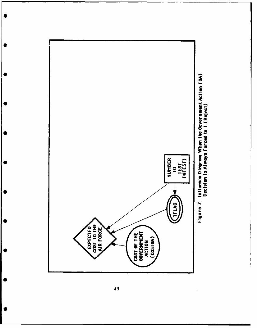
In the second step, the influence diagram is changed so that the

government is always forced to reject whatever degree of nonconformance

* is present and pay the costs of corrective action (whatever that may

be). This is equivalent to always forcing GA to be 1 (reject). See

Figure 7 for the influence diagram when GA is forced to 1.2

Next, a three level, 3 full factorial experiment is performed on

both of the modified models. The probability distribution on the cost

of corrective action (COSTGA) is not changed so that it maintains a

* mean of $80,000 throughout both experiments. A regression is performed

43

z

00

V) 00

• , _

4c 61

44

*-

C

*6

uj0

* c

- z

0j

45

on the data from the experiments of both z'f the modified models.

Now each of the regression equations from each of these modified

models defines a surface in three dimensions. The variables TPG and

DAMGBP make up the two horizontal axes and the response, expected cost

to the Air Force, is the vertical axis. If the surfaces defined by

these two regression equations intersect, their line of intersection

can be found and projected onto the plane defined by the TPG and DAMGBP

axes. The usefulness of such a plot is best illustrated by an example.

Example

Forcing GA to be 0 (accept). Figure 6 shows the influence diagram

in which the government action (GA) decision is forced to be 0

(accept). A full factorial experiment was performed using this

influence diagram. The probability distribution for the COSTGA

variable was not changed to a high or medium setting, but rather, the

COSTGA distribution kept it's mean constant at $80,000 throughout the

experiment. Therefore, there are two independent variables and it2

takes 9 runs to do a three level 3 full factorial experiment. The

high, medium, and low settings for each of the means of the TPG and

DAMGBP distributions are:

HIGH (+1) MEDIUM (0) LOW (-1)

TPG 0.90 0.85 0.80DAMGBP $150,000 $100,000 $50,000

The standard deviations of each distribution are held constant

throughout the experiment.

46

Standard Deviation

TPG 0.05

DAMGBP $25,000

See appendix B for the variable settings and the output values for

each of the nine runs. A regression is performed against the data from

appendix B and the following regression equation gives a perfect fit

against the data.

Y = -lO,000 + 50,000*TPG - 75,000*DAMGBP + 25,000*TPG*DAMGBP (3)

Note that the above equation is for the coded values of TPG and DAMGBP.

The uncoded equation is:

Y = -150,000 + 50,000*((TPG - 0.85) / 0.05)

- 75,000 * ((DAMGBP - 100,000) / 50,000)

* + 25,000 * ((TPG - 0.85) / 0.05)

* ((DAMGBP - 100,000) / 50,000) (4)

The surface defined by equation (4) is shown as Figure 8. Notice

that the ranges of the two horizontal axes, TPG and DAMGBP, do not

extend past the high and low settings used in the experiment.

Forcing GA to be 1 (reject). Figure 7 shows the influence diagram

in which the government action (GA) decision is forced to be 1

(reject). It is unnecessary to perform a full factorial experiment

using this influence diagram because when GA is forced to 1 (reject),

the expected cost to the Air Force will always be the mean of the

COSTGA distribution. In this case, the mean of the distribution of the

• cost to the government variable (COSTGA) is $80,000. Therefore, the

47

000

00

4~4410.

00

0

-4

48

equation which defines the output for this influence diagram is:

Y = -80,000 (5)

The surface defined by equation (5) is shown as Figure 9.

For this particular example, the surfaces defined by equations (4)

and (5) intersect; see Figure 10. In this instance, one alternative

does not dominate the other. However, in some instances, one

alternative will completely dominate the other alternative in the area

of applicability. In that case, there would be no line of

intersection.

The equation of the line where the two surfaces intersect can be

found by simultaneously solving equations (4) and (5). Solving for

DAMGBP gives:

DAMGBP=[50,000*(70,000-50,000((TPG-0.85)/0.05))] + 100,000(-75,000+25,000((TPG-0.85)/0.05)) (6)

The line defined by equation (6) is plotted as Figure 11. In Figure

11, the line where the two surfaces intersect is projected down onto

the TPG-DAMGBP axis.

The plot has a single line which divides the space into two

regions. In one region, the 'accept' alternative is optimal, and in

the other region, the 'reject' alternative is optimal. The line can be

thought of as a sort of 'break-even line'. On this line, the expected

value of the 'accept' alternative is the same as the expected value of

the 'reject' alternative.

49

0'

6 Ogoo

* ~oooo,

0 0'

c',

00

~o

ol

50

00C

-00010

0O000 0

too

0, 4- 0

0 0 0

00

51

* 0 E-i I

L.M

V))

0 co d

00* hLA.

LWJ

u u

* z

o% co P10 00

* d99M.lY

52

When a plot such as the one in Figure 11 is constructed, it should

help the decision maker determine which decision (accept or reject) is

best. Such a plot can help the decision maker visualize where present

circumstances put him in relation to the 'break-even line'. B

entering the plot for a certain value of TPG and DAMGBP, the decision

maker can see in which region he falls and how close he is to the

'break-even line'. Hopefully, the decision maker will have some

* preconceived notion as to what the true values of TPG and DAMGBP are.

If so, the decision maker can tell if he is close to the line or not.

If his preconceived notions of TPG and DAMGBP put him close to the

line, then more time should bA spent in getting better estimates for

TPG and DAMGBP if it has not already been done.

For example, if the decision maker believes that about 85% of his

parts conform to specifications (TPG), and that, on average, a single

nonconforming part will cause about $55,000 worth of damage (DAMGBP),

then he knows that he is very close to the 'break-even line'. He

should then do one of two things. One, he could get better estimates

for TPG and DAMGBP if he is unsure about them because any error in

their estimates could change the optimal alternative for GA. Or, two,

now that he knows that he is close to the 'break-even line', he knows

that the expected value of his decision will be nearly the same no

matter which alternative he chooses for GA. In light of this, the

decision maker may want to base his decision on the other intangible

political aspects of the problem which are not included in this model

of the technical problem.

53

On the other hand, if the decision maker believes that

significantly less than 85% of his parts conform to specifications, and

that, on average, a single nonconforming part will cause significantly

more damage than $55,000, then he knows he is not close to the 'break-

even line'. The decision maker can then use Figure 11 to see that

according to this technical model of the problem, his optimal

alternative is to reject the batch of parts. Choosing the other

'nonoptimal' alternative is likely to greatly increase the expected

cost to the Air Force.

54

VI. Conclusions

This study developed a prototype model of the nonconforming parts

decision problem which faces AFLC. The model is in the form of an

influence diagram which contains two decisions: the number of items

from the NSN that should be sampled and tested for conformance to

specifications; and, the action that AFLC should take to minimize the

cost to the Air Force.

Lack of Real Data

The model takes a very broad view of the problem. The costs that

are used as variables in the model are aggregates of many other costs

and unknowns. If real data exists that could be used to quantify any

of these unknown variables, then using the real data would be the best

method to continue the analysis. However, it is most likely that true

data does not exist on any of the variables that are used in this

model, and in that case, the only logical way to quantify these

unknowns is to use the subjective opinions of experts. The lack of

real data on a variable does not justify excluding that variable from

the model if it has an important impact on the decision problem. The

variable must still be quantified the best way possible, and that is

through the use of subjective probability assessments from the decision

maker and/or the person who knows the most about the unknown variable.

Uses of the Model

The model developed in this study is only a prototype. However,

the type of results obtainable from using a full blown version of this

55

model could be of great use to certain decision makers within AFLC.

The model explained in chapter III is helpful because it accounts for

those variables which are hard to quantify yet are so important to the

decision that needs to be made. The plot such as the one in Figure 11

* is very useful to the decision maker who is contemplating action and

needs to make a good decision in a short amount of time. Instead of

relying on the accuracy of subjective probability assessments on the

key unknown variables, Figure 11 shows the unknown variables over their

whole range and how they affect the optimal decision. Instead of

having to make extra runs of the model in order to answer 'what if'

questions, the decision maker can look at Figure 11 and see what effect

changing a variable would have.

It is important to note that the results obtained in chapter V not

only give information about the value of the expected cost to the Air

Force based on the values of the inputs, but it also shows how the

optimal decision alternative changes as the unknown variables change.

* If the decision maker has some prior knowledge about the unknown

variables, even if it is purely subjective, he can graphically see

where present circumstances place him with respect to the 'break-even

* line'.

The results of the sensitivity analysis were also very

enlightening. Uncertainty about the true value of DAMGBP has a much

* larger impact on the cost to the Air Force than uncertainty about TPG.

The implication is that it is more important to accurately quantify

DAMGBP than TPG. However, it takes manpower and resources to

* accurately quantify an unknown and subjective variable. Therefore, if

56

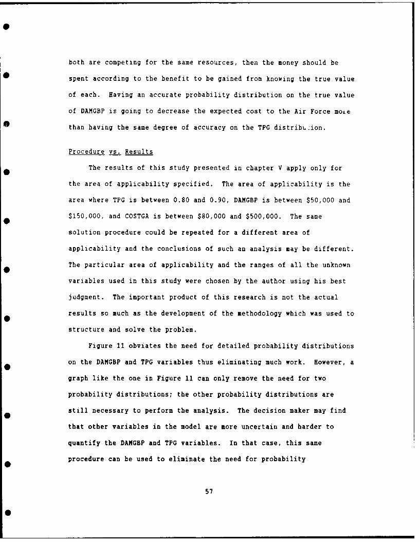
0

both are competing for the same resources, then the money should be

spent according to the benefit to be gained from knowing the true value

of each. Having an accurate probability distribution on the true value

of DAMGBP is going to decrease the expected cost to the Air Force moLe

than having the same degree of accuracy on the TPG distribuLion.

Procedure vs. Results

The results of this study presented in chapter V apply only for

the area of applicability specified. The area of applicability is the

area where TPG is between 0.80 and 0.90, DAMGBP is between $50,000 and

$150,000, and COSTGA is between $80,000 and $500,000. The same

solution procedure could be repeated for a different area of

applicability and the conclusions of such an analysis may be different.

The particular area of applicability and the ranges of all the unknown

variables used in this study were chosen by the author using his best

judgment. The important product of this research is not the actual

results so much as the development of the methodology which was used to

structure and solve the problem.

Figure 11 obviates the need for detailed probability distributions

on the DAMGBP and TPG variables thus eliminating much work. However, a

graph like the one in Figure 11 can only remove the need for two

probability distributions; the other probability distributions are

still necessary to perform the analysis. The decision maker may find

that other variables in the model are more uncertain and harder to

quantify the DAMGBP and TPG variables. In that case, this same

procedure can be used to eliminate the need for probability

57

distributions on the two most uncertain and hardest to quantify

variables.

Necessary Improvements

This model relies heavily on the subjective inputs from experts,

that is why it is so important to spend the effort to perform thorough

probability assessments. It is very important not only to perform

accurate probability assessments, but also to interview as many of the

'experts' as possible so that their differences can be compared and

resolved. The science of combining expert opinions would be extremely

applicable for this task.

The model needs to be made more user friendly so that an expert

can provide the information that the model requires. The model

requires information about two types of random variables. Two of the

random variables which are input to the model can be identified by the

user as more uncertain and more important than the other random

variables. Call these the 'A' variables. Probability distributions

must be built for the rest of random variables which are input to the

model. Call these the 'B' variables.

For the 'A' variables, the user should be able to designate the

ranges over which these random variables are to vary. Instead of being

limited to a probability distribution about these 'A' variables, the

user only has to give a high and a low value for each 'A' variable. In

0 the example in this thesis, DAMGBP and TPG are the 'A' variables. The

decision tool should then take the high, medium, and low values of the

ranges given for the 'A' variables and, using the RSM techniques

* described in this thesis, generate the required runs from the model,

58

0|

and build the appropriate response surface.

Probability distributions will have to be built for the other 'B'

random variables. Most people have a hard time transforming their true

knowledge about an unknown event to numbers which describe a

probability distribution. This author believes the most efficient and

promising method of getting the opinions of experts would be through

the use of a computerized graphical display. It should be similar to

probability wheels which are used when a decision analyst conducts a

personal interview with an expert. Such a graphical display should be

used to enable the decision maker or his designated expert to provide

their knowledge about a subjective event in such a way that the expert

does not require any knowledge about probability or statistics.

Artificial Intelligence should be used in order for the machine to

learn and build the appropriate probability distribution based on the

inputs it receives from the expert or the decision maker.

Finally, the model needs to be expanded to include realistic

alternatives for the government action (GA) decision and for the number

to test decision (NTEST).

59

Appendix A: Data Used in Chapter IV- Output from the Runs Used for Sensitivity Analysis

RUN NUMBER TPG DAMGBP COSTGA OUTPUT VALUE

0 1 -1 -1 -1 $ -80,0002 0 -1 -1 $ -75,0003 1 -1 -1 $ -50,0004 -1 0 -1 $ -80,0005 0 0 -1 $ -80,0006 1 0 -1 $ -80,0007 -1 1 -1 $ -80,0008 0 1 -1 $ -80,0009 1 1 -1 $ -80,000

10 -1 -1 0 $-100,00011 0 -1 0 S -75,O 012 1 -1 0 $ -50,000

0 13 -1 0 0 $-200,00014 0 0 0 $-150,00015 1 0 0 $-100,00016 -1 1 0 $-290,00017 0 1 0 $-225,00018 1 1 0 $-150,00019 -1 -1 1 $-100,00020 0 -1 1 $ -75,00021 1 -1 1 $ -50,00022 -1 0 1 $-200,00023 0 0 1 $-150,00024 1 0 1 $-100,000

" 25 -1 1 1 $-300,00026 0 1 1 $-225,00027 1 1 1 $-150,000

60

Appendix B: Data Used in Chapter VVariable Settings and Output Values

RUN NUMBER TPG DAMGBP COSTGA OUTPUT VALUE

1 -1 -1 -1 $-100,0000 -1 -1 $ -75,000

3 1 -1 -1 $ -50,0004 -1 0 -1 $-200,0005 0 0 -1 $-150,0006 1 0 -1 $-10010007 -1 1 -1 $-300,0008 0 1 -1 $-225,0009 1 1 -1 $-150,000

61

Bibliography

1. Cochran, William G. Sampling Techniques. New York: John Wiley &Sons, Inc., 1953.

2. Department of the Air Force. United States Air Force Budget BookFY 1988/1989 (Amended). Washington: HQ USAF, April 1988.

3. Fertig, Kenneth W. and Nancy R. Mann. "Pample Sizes for VariablesSampling Plans Based on a Decision Theoretic Approach," Journal ofQuality Technology, 15: 63-67 (April 1983).

4. King, Benjamin F. "Surveys Combining Probability and Quota Methodsof Sampling," Journal of the American Statistical Association, 80:890-896 (December 1985).

5. McKalip, Bruce G, Logistics Management Specialist. Personalinterviews. HQ Air Force Logistics Command/MMTQR, Wright-PattersonAFB OH, May through November 1988.

62

VITA

Captain Matthew A. Stone

He graduated from the United States Air Force

Academy in May 1984 with the degree of Bachelor of Science in

Operations Research, and a commission in the USAF. Upon graduation, he

served as an Airborne Warning and Control System Operations Research

Analyst in the Directorate of Operations and Requirements, 28th Air

Division, Tinker AFB, Oklahoma, until entering the School of

Engineering, Air Force Institute of Technology, in May 1987.

63

UN 'LASSIFIEDSEUR:, AS;IICATIOtN O THIS "AGE

SForm A.pproved

REPORT DOCUMENTATION PAGE 0M8 o, 0704-0188

Ia. REPORT SECURITY CLASSIFICATION It. RESTRILTIVE MARKINGS

UNCLASSIl'IED2a. SECURITY (LASSIFICATION AUTHORITY 3. DISTRIBUTIONIAVAILABILIIY OF REPORT

Approved for public release;2b. DECLASSIFICATION/DOWNGRADING SCHEDULE distribution unl imited.

4 PERFORM,'.I ORGANIZATIO :-EPORT NUMBER(S) 5 MONITORING OPGANIZATION REPO;,% NUMbERS)

AFIT/GOR/A/SD-6

6a. NAME OF PERFORMING C G;NIZATI0N 6b. OFFICE SYMBOL 7a. NAME OF MONITORING ORGANIZATION(If applicable)

School of Engineering AFIT/ENC6-. ADDRESS (City, State, and ZIP Code) 70. ADDRESS (City, State, and ZIP Code)

Air Force Institute of Technology (AU)Eright-Patterson AFB OH 45433-6583

8a. NAM- 0: FUNDNG /SPONSORING 1Bb. OFFICE S .:ABOL 9. PROCUREMENT INSTRUMENT IDENTIFICATION .UMBERORGANIZATION (If applicable)HQ AFLC AFLC/M[-ITQR

Ec. ADDRESS (City, State, and ZIP Code) 10. S JURCE OF FUNDING NUMBERS

Air Force Logistics Command PPO%.'RAM I PROJECT ITASK jWORK L:.;TWright-Patterson AFB OH 45433-6583 ELE. ENT NO. NO. NO. ACCESSION NO.

11. TITLE (Include Security Classification)

DECREASING NONCONFORMANCE OF PARTS IN THE AIR FORCE SUPPLY SYSTEM (UNCLASS)

12 PERSONAL AUT.HOR(S)

Matthew A- Stone, B.S., Caot,.USAF13a. TYPE OF REPORT 13b. TIME COVERED 14. DATE OF REPORT (YearMonthOay) 15. PAGE COUNT

MS Thesis IFROM TO___7 1988 Decemb'er 72f16. SUPPLEMENTARY NOTATION

17. COSATI CODES 18. SUBJECT TERMS (Continue on reverse if necessary and identify by block number)

FIELD GROUP SUB-GROUP DECISION MAKING, DECISION THEORY, RESPONSE,i 05 01 LOGISTICS, DECISION ANALYSIS

19. ABSTRACT (Continue on reverse if necessary and identify by block number)

Thesis Advi3or: Joseph A. Tatman, Captain, USAFAssistant Professor, Dept of Mathematics and

Computer Science

20. D!S7RiBUTIONIAVAILA5:LITY OF ABSTRACT 21. ABSTRACT SECUR:TY CLASSIFICATIONEl UCLASSIFIEDPjNLIMtTED C- SAME AS R=T. 0] DTIC USERS UNCLASSIFIED

22a..N.ME OF RESPONSIBLE INDIVIDUAL 22o. TELEPNONE (Include Area Code) 22c. OFFICEt SYMBOLJcseoh A. Tatman, Cantain, USAF L 13)255-3098 AFIT/NC

.. . .. al 25 T lie I T .. .

DD Form 1473, JUN 86 Plevious editions are obsolete. SECURITY CLASSIFICATION OF TI$ PAG-

UNCLASSIFIED

UNCLASSIFIED

Abstract

The purpose of this study was to provide AFLC (Air Force Logistics

Command) with a prototype decision model which will help AFLC engineers

decide when post-production testing for a particular NSN (National

Stock Number) is beneficial to the Air Force, as well as what action

the Air Force should take as a result of that testing. The problem is

a two sided issue. On one hand, nonconformance costs the Air Force in

terms of damaged equipment and potential harm to personnel. On the

other hand, the Air Force cannot afford to test everything. The study

provides an initial step in developing a decision aid to help AFLC

allocate its scarce testing resources.

Sensitivity analysis was performed on this model by using the

techniques of Response Surface Methodology. For the data used in this

study, the random variable which has the greatest impact on the ex-

pected cost to the Air Force is the expected dollar value that a single

part can be expected to cause given that the part is in nonconformance

with its specifications. This result was confirmed using traditional

EVPI (expected value of perfect information) calculations.

The most significant contribution of this study is the development

of a'graphic decision aid. With this aid, the decision maker can

graphically see how the present situation relates to a 'break-even

line', or indifference curve. In addition to showing the decision

maker which alternative is optimal, this method shows how much the

independent variables would have to change for the optimal alternative

to change.UNCLASSIFIED