SEDIMENT IN ARROYO PASAJERO

AND SAN LUIS CANAL

PREPARED FOR: US BUREAU OF RECLAMATION

DENVER, COLORADO

CALIFORNIA DEPARTMENT OF WATER RESOURCES SACRAMENTO, CALIFORNIA

PREPARED BY: PIERRE Y. JULIEN

AUDREY MENDELSBERG COLORADO STATE UNIVERSITY

ENGINEERING RESEARCH CENTER DEPARTMENT OF CIVIL ENGINEERING

FORT COLLINS, COLORADO 80523

July 2003

ii

EXECUTIVE SUMMARY In March of 1995, snowmelt originating in the Diablo Mountain Range flowed along Arroyo Pasajero, before ending up at the San Luis Canal. The floodwaters submerged neighboring farmland and a nearby military base. The flooding wiped out a tomato crop as floodwaters breached the San Luis Canal levee and filled the sediment basins with a mixture of water, sediment, and asbestos. The flooding in 1995 prompted the California Department of Water Resources to consider mitigation design alternatives. The United States Bureau of Reclamation’s Denver office developed a one-dimensional unsteady flow model to simulate the routing of floodwaters through the system. As part of the design alternatives, the sediment basins would be enlarged. This study focuses on sedimentation in the West Side Detention Basins adjacent to the San Luis Canal and on sediment concentrations and transport within the San Luis Canal.

The Arroyo Pasajero carries large quantities of clay. Flocculation tests show that sediment in the area flocculates and most sediment settles at fall velocities exceeding 0.2 mm/s in Arroyo Pasajero and 0.48 mm/s in the San Luis Canal. Two large sediment basins located west of the San Luis Canal pond water and trap sediment carried downstream by the Arroyo Pasajero. The trap efficiency of the detention basins is about 100% for sand and gravel and at least 90% for silt, clay and asbestos. Floodwaters will deposit large amounts of sediment, thus causing the sediment basins to fill over time. Floodwaters may enter the San Luis Canal through inlet gates located near Gale Avenue. The amount of sediment entering the San Luis Canal through inlet gates should not be of any concern and should remain small compared to sediment inflows from Salt Creek and Cantua Creek located upstream on the San Luis Canal.

In the San Luis Canal, dimensionless concentration profiles were calculated for

different size fractions under different flow conditions. The concentration profiles for high flow are fairly uniform with near-surface concentrations at least 60% of the near-bed concentrations. At low flow, the San Luis Canal between Highway 198 and Jayne Avenue traps about 85% of the incoming sediment. At high flows, however, only about only about 30% of the sediment will be trapped, and except for sands, all size fractions are fairly well mixed over the vertical. Daily bedload and total load calculations show that the canal has the ability to transport about 10 cubic yards of sediment at low flow. At a high flow, the daily sediment load will be about 100 cubic yards for bedload and 10,000 cubic yards of total load.

Two main conclusions pertaining to the project can be made. First, the West Side Detention Basins are adequately designed. Second, at high flows in the San Luis Canal, all fractions but sand will be well mixed over the vertical. This allows for a direct diversion of water and sediment to Westlake Farms during flodds. The possibility of using near-surface sluices near Check 21 is considered feasibile and bottom sluices are not necessary when operating the canal at high discharges. At low flow, such sediment diversions would not be possible because the canal would act as a sediment trap.

iii

TABLE OF CONTENTS

LIST OF FIGURES ............................................................................................................ v

LIST OF TABLES.............................................................................................................. 1

1.0 INTRODUCTION ....................................................................................................... 2

2.0 THE AREA OF STUDY ............................................................................................. 3

2.1 The San Luis Canal/ California Aqueduct ............................................................... 3 2.2 Arroyo Pasajero ....................................................................................................... 4

3.0 BACKGROUND ......................................................................................................... 9

3.1 Monitoring Programs............................................................................................... 9 3.2 Asbestos ................................................................................................................. 10 3.3 Alluvial Fan ........................................................................................................... 11 3.4 Flooding ................................................................................................................. 12 3.5 Response of the State to Flooding ......................................................................... 13 3.6 Results of Sediment Testing .................................................................................. 14

4.0 SEDIMENTATION................................................................................................... 15

4.1 Hydraulics .............................................................................................................. 15 4.2 Concentration Profiles ........................................................................................... 16 4.3 Sedimentation ........................................................................................................ 19

5.0 MODEL INPUTS ...................................................................................................... 21

5.1 Arroyo Pasajero ..................................................................................................... 21 5.2 California Aqueduct............................................................................................... 22

6.0 RESULTS .................................................................................................................. 23

6.1 Arroyo Pasajero ..................................................................................................... 23 6.2 California Aqueduct............................................................................................... 25

7.0 CONCLUSION.......................................................................................................... 28

REFERENCES ................................................................................................................. 29

LIST OF PARAMETERS ................................................................................................ 30

Appendix A – Flocculation Testing.................................................................................. 31

iv

Appendix B –Sediment Concentration Profiles................................................................ 37

v

LIST OF FIGURES

Figure 1: California State Water Project Map .................................................................... 3

Figure 2: Map of the Area Showing Tributaries of Arroyo Pasajero ................................. 4

Figure 3: El Dorado Avenue Looking Downstream and Upstream.................................... 5

Figure 4: Lassen Avenue Looking Upstream at Low Flow and High Flow Channels ....... 5

Figure 5: Lassen Avenue Looking Downstream ................................................................ 6

Figure 6: Radial Gates Located South of the Railroad Tracks along San Luis Canal ........ 6

Figure 7: Sediment Basins at Railroad Looking Upstream and Downstream .................... 7

Figure 8: Evacuation Culvert Located in Sediment Basin near Railroad ........................... 7

Figure 9: Front View of Inlet Gates Located at Gale Avenue ............................................ 8

Figure 10: Monitoring Stations in Arroyo Pasajero (Faria, 1992)...................................... 9

Figure 11: Location of Alluvial Fan ................................................................................. 11

Figure 12: 1995 Flooding.................................................................................................. 13

Figure 13: Sediment Testing Locations ............................................................................ 14

Figure 14: Picture of Upper, Middle and Lower Sediment Basins................................... 21

Figure 15: Sediment Distribution from Bedload Sample taken Downstream of Lassen Ave............................................................................................................................ 23

1

LIST OF TABLES

Table 1: Percent Composition and Classification............................................................. 14

Table 2: Classes of Sediment............................................................................................ 16

Table 3: Current Upper, Middle and Lower Sediment Basin Characteristics .................. 21

Table 4: Proposed Upper, Middle and Lower Sediment Basin Characteristics.. 22 Table 5: Grain Sizes Used in Calculations.............................................................................. 22

Table 6: Key Variables in San Luis Canal at Range of Flows.......................................... 22

Table 7: Key Properties in Trap Efficiency Calculations ................................................. 23

Table 8: Maximum Velocity Trap Efficiency Calculations for the Current Conditions .. 24

Table 9: Maximum Depth Trap Efficiency Calculations for the Current Conditions ...... 24

Table 10: Maximum Velocity Trap Efficiency Calculations for the Proposed Conditions................................................................................................................................... 25

Table 11: Maximum Depth Trap Efficiency Calculations for the Proposed Conditions.. 25

Table 12: Rouse Numbers at Range of Flows ................................................................. 25

Table 13: Trap Efficiency at Low Flow............................................................................ 26

Table 14: Trap Efficiency at Intermediate Flow............................................................... 26

Table 15: Trap Efficiency at High Flow........................................................................... 26

Table 16: Bedload Concentration and Flow Rate for Range of Flows ............................. 27

Table 17: Total Load Concentration and Flow Rate for Sand Particles ........................... 27

2

1.0 INTRODUCTION

The State of California is made up of a system of streams, lakes, rivers and Aqueducts. The stream of interest in this study is Arroyo Pasajero. The participants in this study include Colorado State University (CSU), the Bureau of Reclamation (Reclamation) and the California Department of Water Resources (DWR).

Arroyo Pasajero is a small arroyo originating in the Diablo Mountain Range.

Floodwaters travel east towards the San Luis Canal where they reach a series of sediment basins. The sediment basins have filled with sediment over the years, depleting the amount of storage available for floodwaters. In 1995, a large flood passed along Arroyo Pasajero, breaching the San Luis Canal Levee and entering the San Luis Canal. Flood inflows carry large amounts of asbestos causing concerns for engineers.

As a result of the 1995 flooding, DWR and Reclamation have began looking at

design alternatives. DWR has determined a new design for the sediment basins to increase the amount of storage. Reclamation has developed a one-dimensional unsteady flow model to route the floodwaters and minimize flooding in neighboring properties. Colorado State University was brought into the project as a sedimentation consultant to aid Reclamation.

The analysis specifically looks at sediment concentration profiles and trap

efficiency of both sediment and asbestos within the San Luis Canal. In addition, trap efficiency within the sediment basins will be determined. Finally, an estimate of both bedload and total load will be carried out to give aqueduct designers an idea of the amount of sediment passing through the system.

This report describes the sedimentation analysis carried out at Colorado State

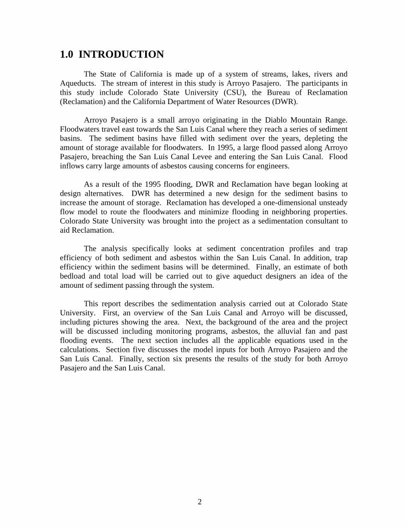
University. First, an overview of the San Luis Canal and Arroyo will be discussed, including pictures showing the area. Next, the background of the area and the project will be discussed including monitoring programs, asbestos, the alluvial fan and past flooding events. The next section includes all the applicable equations used in the calculations. Section five discusses the model inputs for both Arroyo Pasajero and the San Luis Canal. Finally, section six presents the results of the study for both Arroyo Pasajero and the San Luis Canal.

3

2.0 THE AREA OF STUDY

2.1 The San Luis Canal/ California Aqueduct The San Luis Canal, a joint use facility for California and the Federal

Government, is a 102-mile long segment of the California Aqueduct and an important element of the overall State Water Project (SWP). As can be seen from Figure 1, the SWP covers most of the state. The SWP is a series of reservoirs, aqueducts, powerplants, and pumping plants whose purpose to distribute water to 29 urban and agricultural water contractors and 17 other agencies. Of the water supply, 30 percent is for agricultural use and 70 percent is for urban use. The project helps control flood levels, enhance fish and wildlife, increase recreational opportunities and improve water quality in the Sacramento-San Joaquin Delta. This large-scale project services two-thirds of California’s population. The system is maintained and operated by the California Department of Water Resources (DWR). The system was originally designed to manage the water system as the population within many of the cities grew.

DWR currently monitors 32 reservoirs, lakes and storage facilities; 17 pumping

plants; 3 pump-generating plants; 5 hydroelectric power plants; and about 660 miles of pipelines and open canals (http://www.water.ca.gov/swp/history.html).

Figure 1: California State Water Project Map

(http://www.water.ca.gov/swp/facilities/water)

Figure 1 shows the complexity of the water system. The SWP starts in Northern California on the Upper Feather River. The water flows into the Oroville-Thermalito

4

area. In this area is a large dam which can store about 3.5 million acre-feet (MAF) called the Oroville Dam. The majority of this available storage is used for the water supply; however, about 800,000 AF is used to help alleviate downstream flooding. The flow is divided as it reaches the Sacramento-San Joaquin Delta area. Part of the water is pumped along the North Bay Aqueduct to the local counties. The other part of the divided water travels through a pumping plant and then down the California Aqueduct. The 444-mile long California Aqueduct travels approximately 63 miles to the San Luis Reservoir. This reservoir, jointly operated by the Department and the Central Valley Project (USBR), has a total storage of 2.04 MAF of which 971,000 AF is reserved for federal water.

Flow continues to the southern San Joaquin Valley where along the way water is diverted for San Luis Obispo and Santa Barbara. As the water enters the Tehachapi Mountains, another power plant raises the water 1,926 feet to a sequence of tunnels and siphons that traverse the range. On the other side of the mountains, the water divides into two branches. The West Branch Aqueduct stores water in two reservoirs to serve Los Angeles and the other coastal cities. The East Branch Aqueduct reaches Silverwood Lake first and then travels to its final destination in the Lake Perris reservoir (http://www.water.ca.gov/swp/facilities/water).

2.2 Arroyo Pasajero The Arroyo Pasajero is a naturally flowing stream located in central California.

The flow originates from spring storms in the Diablo Mountain Range and passes a few cities including Coalinga and Huron. Downstream of Huron, the incised channel terminates as the Arroyo Pasajero fans out and enters a set of detention basins and then the San Luis Canal. There are four main tributaries of Arroyo Pasajero: Los Gatos Creek, Warthan Creek, Jacalitos Creek, and Zapato Chino Creek. Figure 2 shows the tributaries and the area of study.

Figure 2: Map of the Area Showing Tributaries of Arroyo Pasajero

As Arroyo Pasajero flows towards the San Luis Canal it flows across a few streets. One of the first roads that it crosses is El Dorado Avenue. In this area, the channel has become incised. The top layer of sediment is composed of silts and clays. During times of high flow, this top layer is transported downstream causing scour holes

5

that may become a few feet deep. These scour holes have undermined the bridge piers at El Dorado Avenue. Figure 3 shows Arroyo Pasajero looking both upstream and downstream.

Figure 3: El Dorado Avenue Looking Downstream and Upstream

Traveling downstream, the next road that Arroyo Pasajero will meet is Lassen Avenue. Lassen Avenue has two different channels for low and high flows. The low flow channel has five small culverts used to transport water underneath Lassen Avenue. During times of high flow, the water will travel through a much larger open area with levees to help control the water. The low flow and high flow channels looking upstream can be seen in Figure 4.

Figure 4: Lassen Avenue Looking Upstream at Low Flow and High Flow Channels

Once the water flows under (during low flow conditions) or over (during high flow conditions) Lassen Avenue it continues through an open area. The majority of the water will travel through a smaller channel located on the right hand side of Figure 5. This channel will help align the flow with the sediment basins located along the San Luis Canal. Estimates suggest that this area has subsided by about 30 feet between the 1920’s and 2002.

6

Figure 5: Lassen Avenue Looking Downstream

The water travels along a training dike located just South of Highway 198. The dike helps keep the water from flooding farmland located to its north. Figure 6 shows a set of three radial gates along the San Luis Canal located north of the San Joaquin Valley Railroad.

Figure 6: Radial Gates Located South of the Railroad Tracks along San Luis Canal

The raised railroad tracks running parallel to the San Luis Canal have been redone many times due to the flooding. The floodwaters that pass under the railroad tracks have deposited a large amount of sediment causing a reduction in passage. The department of water resources has to excavate the sediment from underneath the bridge. The sediment basins on the upstream and downstream side of the railroad can be seen in Figure 7. The area farthest east (closest to the aqueduct) is all sediment without any vegetation. As you travel west, more shrubbery and small trees are present. The town of Huron, California can be seen in the distance on the upstream picture.

7

Figure 7: Sediment Basins at Railroad Looking Upstream and Downstream

Located in the sediment basins to the north of the railroad tracks is an evacuation culvert. The culvert will transport water from the sediment basins to the fields on the other side of the San Luis Canal. When this occurs not only is the farmland flooded, but an air force base also may become flooded. The evacuation culvert can be seen in Figure 8.

Figure 8: Evacuation Culvert Located in Sediment Basin near Railroad

Gale Avenue is the levee for the sediment basins at the downstream end. At this location, there are a set of inlet gates to move water out of the sediment basins and into the San Luis Canal. There are 12 inlet gates into the San Luis Canal. There are four locations where water can enter the canal with three gates at each of these locations. Figure 9 shows a front view (looking east) of these inlets.

8

Figure 9: Front View of Inlet Gates Located at Gale Avenue

9

3.0 BACKGROUND

The San Luis Canal obstructs the sediment and water flow of Arroyo Pasajero. Several facilities were built to disperse and pond Arroyo Pasajero during San Luis Canal construction and to handle future flooding. One facility was a basin on the Aqueduct’s west side and east of State Highway 198, between a training dike from the north and Gale Avenue from the south. The original design capacity of the basin is 18,500 acre-feet. Another facility is an evacuation culvert that can drain water from the basin and disperse it on the Aqueducts east side. The final facility is twelve inlet gates that can release the ponded water from the basin into the Aqueduct during emergencies to prevent the Aqueduct west embankment from being overtopped. In the last 10 to 20 years, it has become obvious that the floodflows associated with the Arroyo Pasajero pose a threat to the Aqueduct and the surrounding area. The Arroyo Pasajero flows contain more sediment than designers expected causing depletion in basin storage. The flows originating in the upper reaches of the Arroyo Pasajero watershed have a high concentration of asbestos. During the spring months and other high precipitation events, the flows can overtop the Aqueduct’s west embankment, flood surrounding farmlands and impact downstream residents.

3.1 Monitoring Programs An extensive monitoring program, developed in 1991, gathers information necessary to define the flow and sediment transport characteristics of Arroyo Pasajero. A number of stations were set up throughout the entire watershed to collect precipitation, streamflow and sediment data. Figure 10 shows the locations of these stations within the watershed. (Faria, 1992)

Figure 10: Monitoring Stations in Arroyo Pasajero (Faria, 1992)

10

3.2 Asbestos As mentioned previously, there are some areas of the Arroyo Pasajero where large

concentrations of asbestos are prevalent. Asbestos is a naturally occurring mineral found in the Diablo Mountain Range. Through drainage of the watershed, the asbestos fibers are conveyed into streams, lakes, rivers and reservoirs. Concerns about asbestos levels in water are heightened from cases of lung cancer because of airborne asbestos. These concerns caused the Environmental Protection Agency (EPA) to impose maximum contaminant level (MCL) standards for drinking water. The MCL put in place by the EPA in 1985 was seven million fibers per liter (MFL) that are longer than 10 microns for filtered drinking water. The EPA does not have a regulation in place for raw water.

Asbestos monitoring within the Arroyo Pasajero watershed originated in the early 1980’s. This was a result of high levels of asbestos in the California Aqueduct deliveries. The levels of asbestos in the headwaters of the Aqueduct were significantly lower than those downstream of the San Luis Canal. The elevated levels were a result of the Arroyo Pasajero flood flows entering the Canal at the Gale Avenue inlet gates and Cantua and Salt Creeks. Cantua and Salt Creek are north of Arroyo Pasajero, their flows enter the Aqueduct at the Mt. Whitney flume and Salt Creek drain inlet, respectively. Cantua Creek is an ungated inlet allowing all water, sediment and asbestos to flow into the aqueduct. Salt Creek has a small gate with a limited capacity of storage. As a result of the discovery of the asbestos in the flows, the Gale Avenue inlet gates are not used for flood control unless necessary. Programs to monitor asbestos levels in the Arroyo Pasajero waters were put in place in 1981; however, a continuous sampling program was not put in place until 1991. The asbestos in the Aqueduct, called chrysotile, was carried there by sediment. Dredging, using a pneumatic pump, was implemented to remove the sediment in the area. Results of the dredging showed a 70 percent reduction in asbestos concentrations. The asbestos sources in the Arroyo Pasajero were further traced to asbestos mines and serpentine outcrops in the Los Gatos Creek watershed. The mines and their tailings were found to intrude on the tributaries of Los Gatos Creek. Mining in the area is believed to have begun in the 1920’s. In the late 1950’s, geologists “rediscovered” the asbestos formations which resulted in a large influx of mining. Two large-scale mining operations were created in the Los Gatos Creek Area. The Atlas mine on the Upper White Creek was in operation until 1974 and the Johns-Manville mine in Pine Creek Canyon was in operation until 1979. Both mines were forced to discontinue operation due to increasing costs related to federal regulations and decreasing sales. (Arroyo Pasajero Feasibility Study Appendix: Water Quality Report)

The serpentine outcrops in the area are part of the New Idria serpentine body. This body contains sheared and crushed materials made up of soft, crumbly aggregates and sheets of asbestos. The serpentinite has little surface strength, and the rounded hills that develop on it are easily eroded. The unstable serpentinite has caused landslides over the area. Electron microscope studies of the asbestos show that the fibers range in length from one to 20 microns with an average of about five microns. (Coleman, 1995) The serpentinite formation covers a 48 square mile area along the Diablo Range with seven square miles of that in the Los Gatos Creek Watershed.

11

Effects of asbestos in drinking water have yet to be determined. The short

chrysotile fibers have a small diameter and a surface that is three to four times greater than larger fiber chrysotile. A study was conducted of about 450 mineworkers in 1963 to determine the affect of the asbestos. As of 1997, physicians have not detected asbestos related medical problems. (Arroyo Pasajero Feasibility Study Appendix: Water Quality Report)

3.3 Alluvial Fan Historically and pre-aqueduct construction, a large alluvial fan has developed on the downstream end of the Arroyo Pasajero and parts of it, currently, is on the east side of the California Aqueduct. The fan has an area of about 450 square miles and is bisected by a seismically active anticline. Figure 11 shows the location of the alluvial fan. The fan, west of the Aqueduct has experienced an extensive amount of channel incision in recent years. The lower fan has experienced as much as 18 feet of land subsidence since the 1920’s. Conversely, the upper fan has remained relatively stable over the years.

Figure 11: Location of Alluvial Fan

The channels within the fan have incised from 10 to 41 feet deep with the majority of the incision in the lower fan and through the anticline gap. The Arroyo Pasajero thalweg elevation has changed little, indicating that subsidence is not an issue in this area. The majority of the channel incision has occurred since 1933 as a direct result of two different phenomena. One of these phenomena is tectonic uplift centered along the anticline. Tectonic uplift is due to earthquakes, which suggests that the incision in the channel evolved gradually and episodically. The second reason for the channel incision is land subsidence in the lower fan. The main source of land subsidence is groundwater

12

withdrawals for irrigation. Base level studies suggest that Arroyo Pasajero will eventually reach a new stable base level sometime in the future (Leclerc, 1997).

3.4 Flooding Flooding along Arroyo Pasajero is a problem for the state of California. The largest storm on record occurred in March of 1969. A volume of about 55,000 acre-feet passed through Arroyo Pasajero. Another storm in 1975 passed about 35,000 acre-feet through Arroyo Pasajero. Storms similar to this occurred in 1975 and again in 1993.

The year 1995 proved to be a problematic year for the state of California. Total floodwater inflows within a portion of the San Luis Canal were 25,932 acre-feet, the second highest on record. The month of March produced over 77 percent of the 1995 inflows (20,054 acre-feet). The Gale Avenue inlet contributed about 4,144 acre-feet.

On March 10, high winds and heavy Aqueduct inflows crested the California Aqueduct levee. At least 20 canal lining panels were destroyed and further flooding was expected in the area. Upstream, on the Arroyo Pasajero, an estimated peak flood flow of 33,000 cfs (a 40-year flood event) occurred around 8:30 am at the Interstate-5 Bridge. The flooding caused deep erosion that undermined the bridge foundation and caused its collapse. Seven people traveling along I-5 died in the collapse.

On March 11, in the Arroyo Pasajero area, record floods greater than 25,000 cfs filled the detention basins to the West of the Aqueduct. This forced the release of 3,000 cfs through the Gale Avenue drain inlets into the Aqueduct. A power outage in the area hampered the release of water through an additional excavation culvert located under the Aqueduct. Once power was restored to the system, the culvert released water at a rate of 1,000 cfs. The release did not occur before overtopping occurred north of the Gale Avenue drain inlet through a large break (resulting from a piping failure) in the west Aqueduct levee. (http://wwwswpao.water.ca.gov/publications/bulletin/96/text/cha6.html) An uncontrolled flow of 300 cfs, corresponding to a volume of about 2,635 acre-feet, entered the Aqueduct through the 50’ by 11’ breach. The breach was not repaired until March 14. (Water Quality Assessment of the State Water Project, 1994-1995) A picture taken right after the 1995 flood can be seen in Figure 12.

The Arroyo Pasajero flooding problems contributed to the shutdown of a water treatment plant located downstream of the drain inlets. High silt loads carried by the inflows, along with a water main break, overwhelmed the filtering capacity of the treatment plant. Adding to the problems, a Chevron oil pipe ruptured in the Arroyo Pasajero watershed on March 10. The rupture produced about 4,400 barrels (180,000 gallons) of crude oil that entered the detention basins. In response to the rupture, Chevron set up oil booms in the basins and at the site of the rupture. The Gale Avenue drain inlet gates were closed as the oil-laden flows approached the Aqueduct. It was determined that organic hydrocarbons were below drinking water MCLs with the exception of benzene. The rates returned to normal in about four days.

13

Figure 12: 1995 Flooding

A large amount of sediment entered the San Luis Canal as a result of the storms. The sediment could be transported downstream as a suspended solid or settled on the Aqueduct invert. The total amount of sediment that passed through the area was estimated to be between 600,000 and 1,400,000 cubic yards. The suspended sediment is detrimental because it causes wear on pump impellers and shafts. The sediment can also be a threat to public health by interfering with water treatment processes. The high turbidity associated with the sediment is also a concern for agricultural drip irrigation operations and groundwater recharge. It is estimated that about 55,000 cubic yards of sediment were removed from the system. There are sand traps located in the Aqueduct to help settle out sediment; however, the system was overwhelmed due to the large amount of sediment present. To aid in the collection of sediment, some dredging took place in 1996. The dredging activity had little or no influence on downstream water quality. (http://wwwswpao.water.ca.gov/publications/bulletin/96/text/cha6.html)

Through time, Arroyo Pasajero has become an incised channel. As a result of the bed material, in times of high flow large scour holes will form. These holes cause problems for bridges and other structures along the way. Over the years, undermining of the bridge footings has caused collapse. The sedimentation basins on the west side of the San Luis Canal have collected all the sediment transported through Arroyo Pasajero. As of 2003, storage has decreased from 16,500 acre-feet with freeboard to about 6,000 acre-feet and no freeboard. The current conditions allow a storm with less than a 5-year flooding event to pass through the area.

3.5 Response of the State to Flooding In response to the flood, a short-term operational procedure was created in case a flood of this magnitude was to occur again. The preferred alternative follows the designated path of floodwaters at the existing retention basins on the west side of the Aqueduct. The path follows the three steps listed below:

1. Impound floodwaters west of the Aqueduct,

14

2. If the water level continues to rise, allow flows to the east of the Aqueduct by using the evacuation culvert, and 3. As a last resort, allow floodwaters to enter the Aqueduct through the drain inlet gates at Gale Avenue. (http://wwwswpao.water.ca.gov/publications/bulletin/95/view/text/cha12.htm)

As a result of the flooding in Arroyo Pasajero, the California Water Commission requested that the Department create an Arroyo Pasajero Multi-Agency Forum. The forum includes public officials, agency representatives and members of the public. The forum will provide early access to study findings and an opportunity for members to participate in the formulation of alternatives for the project. (http://wwwswpao.water.ca.gov/publications/bulletin/96/text/cha12.html)

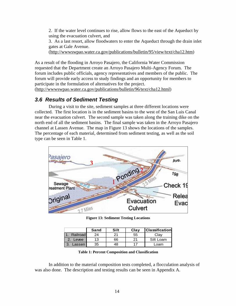
3.6 Results of Sediment Testing During a visit to the site, sediment samples at three different locations were collected. The first location is in the sediment basins to the west of the San Luis Canal near the evacuation culvert. The second sample was taken along the training dike on the north end of all the sediment basins. The final sample was taken in the Arroyo Pasajero channel at Lassen Avenue. The map in Figure 13 shows the locations of the samples. The percentage of each material, determined from sediment testing, as well as the soil type can be seen in Table 1.

Figure 13: Sediment Testing Locations

Sand Silt Clay Classification

1. Railroad 24 21 55 Clay2. Levee 13 66 21 Silt Loam

3. Lassen 35 48 17 Loam Table 1: Percent Composition and Classification

In addition to the material composition tests completed, a flocculation analysis of was also done. The description and testing results can be seen in Appendix A.

15

4.0 SEDIMENTATION The sedimentation calculations can be broken into three different areas of study: Hydraulics, Concentration Profiles, and Sediment. This is also the order in which the calculations occurred.

4.1 Hydraulics First, the velocity in the channel must be calculated using equation (1).

AQV = (1)

Where: V = velocity in m/s Q = flow rate in m3/s A = area in m2 The friction slope is calculated using equations (2) and (3). Equation (2) calculates the Froude number, which is an indicator of the ratio of flow velocity V to surface wave celerity in open channels.

ghVFr = (2)

2

8FrfS f = (3)

Where: Fr = Froude number V = velocity in m/s Sf = friction slope f = Darcy Weisbach friction factor g = gravitational acceleration in m/s2 h = water depth in m

Next, the shear velocity can be calculated using equation (4).

fhSgRu =* (4)

Where: u* = shear velocity in m/s Rh = hydraulic radius in m g = gravitational acceleration in m/s2 Sf = friction slope

16

Equation (4) holds for high flows; however, at low flow conditions, a smooth boundary will form and equation (5) should be used instead.

25.3log75.5 *

*

+⎟⎟⎠

⎞⎜⎜⎝

⎛=

m

huuV

ν (5)

Where: u*= shear velocity in m/s V = velocity in m/s h = water depth in m νm = kinematic viscosity in m2/s

4.2 Concentration Profiles The sediment concentration profiles are another important factor in the

calculations of sediment transport. It is important to determine how much of the sediment will be caught in suspension and where along the depth it occurs. To calculate the suspended sediment, there are a number of equations that must be solved; however, appropriate grain sizes must first be determined. Table 2 shows the classes of sediment along with their diameter, angle of repose, critical shear stress and velocity, and settling velocity.

Table 2: Classes of Sediment

(Julien, 1998)

17

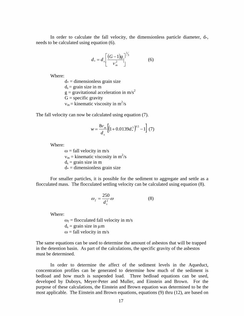
In order to calculate the fall velocity, the dimensionless particle diameter, d*,

needs to be calculated using equation (6).

( ) 31

2*1

⎥⎦

⎤⎢⎣

⎡ −=

ms

gGddν

(6)

Where: d* = dimensionless grain size ds = grain size in m g = gravitational acceleration in m/s2 G = specific gravity νm = kinematic viscosity in m2/s The fall velocity can now be calculated using equation (7).

( )[ ]10139.018 5.03* −+= d

dw

s

mν (7)

Where: ω = fall velocity in m/s νm = kinematic viscosity in m2/s ds = grain size in m d* = dimensionless grain size

For smaller particles, it is possible for the sediment to aggregate and settle as a flocculated mass. The flocculated settling velocity can be calculated using equation (8).

ωω 2

250

sf d

= (8)

Where: ωf = flocculated fall velocity in m/s ds = grain size in µm ω = fall velocity in m/s The same equations can be used to determine the amount of asbestos that will be trapped in the detention basin. As part of the calculations, the specific gravity of the asbestos must be determined. In order to determine the affect of the sediment levels in the Aqueduct, concentration profiles can be generated to determine how much of the sediment is bedload and how much is suspended load. Three bedload equations can be used, developed by Duboys, Meyer-Peter and Muller, and Einstein and Brown. For the purpose of these calculations, the Einstein and Brown equation was determined to be the most applicable. The Einstein and Brown equations, equations (9) thru (12), are based on

18

the concept that bedload transport is controlled by the turbulent flow fluctuations and that grains move in steps proportional to their size. It should be noted that the bedload equations are applicable for a range of flows.

( ) ( ) ( )

1

3

2

3

23

* 136

136

321

−

⎟⎟⎟

⎠

⎞

⎜⎜⎜

⎝

⎛

⎪⎩

⎪⎨⎧

⎪⎭

⎪⎬⎫

−−

−+−=

s

m

s

msbvbv gdGgdG

gdGqq νν (9)

18.0 when15.2 *

/391.0*

* <= − ττeqbv (10) 18.052.0 when40 *

3** >>= ττbvq (11)

0.52 when15 *5.1

** >= ττbvq (12) Where: qbv= bed material in motion per unit width in ft2/s ds= grain size in mm τ*= shields parameter g = gravitational acceleration in m/s2

G = specific gravity νm = kinematic viscosity in m2/s

For purposes or this study, a total load equation was also evaluated. The Engelund and Hansen equation (equation (13)) can calculate the total amount of sand within the system. The amount of silt and clay present in the system was not calculated. If these values were to be calculated, the numbers would be large (order of millions) giving unreasonable and unusable results.

( )[ ] ( )2

1

21 11105.0 ⎥

⎦

⎤⎢⎣

⎡−−

⎟⎠⎞

⎜⎝⎛

−=

s

fh

s

fw dG

SRgdG

VSG

GC (13)

Where: Cw = concentration by weight of sediment G = specific gravity V = velocity in m/s Sf = friction slope g = gravitational acceleration in m/s2

ds = grain size in m Rh = hydraulic radius in m

The Rouse number, equation (14), is the ratio of the fall velocity to the shear velocity.

*0 u

Rβκ

ω= (14)

Where: Ro = Rouse number

19

β = ratio of turbulent mixing coefficient to momentum exchange coefficient

κ = von Karman constant ω = fall velocity in m/s

The final calculation for the concentration profile is equation (15). As part of the calculation, the concentration at a known depth must be calculated. The bedload concentration could be used at a depth of two times the size of the particle. (Julien, 1998)

oR

aha

zzh

CaC

⎟⎠⎞

⎜⎝⎛

−−

= (15)

Where: C = sediment concentration Ca = concentration at a given depth, a h = water depth in m a = depth from channel bed in m z = depth at a given location relative to the channel bed in m

4.3 Sedimentation As a result of continuity of sediment, part of the sediment will deposit on the bed

of the channel as the transport capacity decreases. For the purpose of these calculations, it is assumed that there is a steady supply of sediment and that the diffusive and mixing fluxes are small compared with the advective fluxes in the detention basins. The main advective flux in this case is the fall velocity of the sediment. For gradually varied flow and constant fall velocity, equation (16) could be used.

0=+hC

dxdCvx

ω (16)

Where: vx = velocity in the x-direction in m/s C = sediment concentration x = distance along the channel in m ω = fall velocity in m/s h = water depth in m The trap efficiency, TE, that can be seen in equation (17) is defined as the percentage of a given sediment fraction that settles within a given distance X.

hVX

E eTω−

−= 1 (17) Where: TE = trap efficiency X = distance downstream where a given particle will settle in m

20

ω = fall velocity in m/s h = water depth in m

V = velocity in m/s

21

5.0 MODEL INPUTS

5.1 Arroyo Pasajero In order to determine the percentage of each material that will be trapped in the detention basins (see Figure 14), there were a number of parameters that had to be defined. The peak flow at the I-5 Bridge was used to determine the flow rates present in the three basins. The upper sediment basin had a flow that was 80 percent of the peak flow and the middle and lower sediment basins had flows that were 50 and 20 percent of the peak flow, respectively. The peak flow was 33,000 cfs so the upper, middle and lower sediment basins had flows of 26,400 cfs, 16,500 cfs and 6,600 cfs. The trap efficiency for both the current and the proposed conditions were calculated. The length along the sediment basin was determined from Figure 2. The velocity and depth were determined from the FLO2D model for the sediment basins. The current conditions are summarized in Table 3 and the revised conditions are summarized in Table 4. It should be noted that at this time the SWP only owns the upper and middle sediment basins, referred to as the Westside Detention Basins. The SWP does not own the lower sediment basin at this time although it was flooded during the 1995 flood.

Figure 14: Picture of Upper, Middle and Lower Sediment Basins

Flow Rate Length Width Max

Depth Velocity Max Velocity Depth

Basin Location cfs miles ft ft ft/s ft/s ftNorth Basin 26400 2.5 6000 4.16 0.75 1.5 3.62North of RR 26400 2.5 6000 8.99 0.71 2.46 8.33South of RR 16500 2.7 5500 8.56 0.3 3.75 6.46Gale Ave DI 16500 2.7 5500 9.91 0.37 3.01 9.58

Lower South of Gale Ave 6600 3 5000 14.52 0.03 3.38 5.38

Upper

Middle

Table 3: Current Upper, Middle and Lower Sediment Basin Characteristics

22

Flow Rate Length Width Max

Depth Velocity Max Velocity Depth

Basin Location cfs miles ft ft ft/s ft/s ftUpper North Basin 26400 2.5 6000 4.8 0.56 1.5 4.1

North of RR 26400 2.5 6000 9.31 0.34 2.64 8.28Middle South of RR 16500 2.7 5500 9.79 0.38 4 6

Gale Ave DI 16500 2.7 5500 10.58 0.29 2.22 2.53Lower South of Gale Ave 6600 3 5000 14.2 0.01 1.57 0.91

Table 4: Proposed Upper, Middle and Lower Sediment Basin Characteristics

The grain sizes used in the calculations were determined from Table 3. The “medium” grain size was selected for these calculations. The grain sizes are summarized in Table 5.

Grain SizeClass mmGravel 8Sand 0.25Silt 0.016

Clay 0.001 Table 5: Grain Sizes Used in Calculations

An asbestos length of 10 micrometers, the EPA’s MCL for drinking water, was used in the calculations. The specific gravity, G, of the asbestos in Arroyo Pasajero was determined to be about 2.45. This specific gravity is less than what would be expected for sediment (G = 2.65), but higher than what would be expected for pure water (G = 1) (http://www.smico.com/pdf/mat_density_grav_angle.pdf).

5.2 California Aqueduct The Aqueduct has a slope of 0.00004 along the stretch of concern. The Aqueduct is a trapezoidal channel with a base width of 50 feet (for Pool 20 and 21 only). The channel also has a side slope of 2 to 1 along a distance of 63.8 feet (Railroad crossing drawing). The design flow for the Aqueduct is 8,350 cfs corresponding to a depth of 24.00 feet. A flow of 2000 cfs, referred to herein as the intermediate flow, corresponds to a depth of about 23.20 feet. At low flows of about 500 cfs, the corresponding depth is 23.00 feet. Table 6 summarizes the variables of interest for the range of flows.

Flow Depth Base Width

Top Width Velocity Slope U*

cfs ft ft ft ft/s ft/sLow Flow 500 23.00 50 126 0.27 0.00004 0.0097

Intermediate Flow 2000 23.20 50 162 0.74 0.00004 0.0090High Flow 8350 24.00 50 166.00 2.95 0.00004 0.04

Table 6: Key Variables in San Luis Canal at Range of Flows

In order to calculate the sediment profile for the Aqueduct, a monitoring location within the detention basin was selected. The sediment sample from AP-14-BED-1 (about 2000 feet downstream of Lassen Avenue) has a d15 of 0.105 mm, the d50 was 0.208 mm, the d85 was 0.411 and the d90 was 0.503 mm. Figure 15 shows the sediment distribution for the San Luis Canal (Northwest Hydraulic Consultants).

23

Figure 15: Sediment Distribution from Bedload Sample taken Downstream of Lassen Ave

6.0 RESULTS

6.1 Arroyo Pasajero Before the calculations of trap efficiency were completed, it was necessary to determine the settling velocity of the sediment and asbestos. These values were the same in each of the basins because they are only dependent on the grain size, specific gravity and the kinematic viscosity, properties that were the same in each sediment basin. The results of the calculation are summarized in Table 7.

Grain Size ωClass mm G d* m/sGravel 8 2.65 202.368 3.38E-01

d85 0.411 2.65 10.397 5.99E-02Sand 0.25 2.65 6.324 3.60E-02d50 0.208 2.65 5.262 2.84E-02d15 0.105 2.65 2.656 9.35E-03Silt 0.016 2.65 0.405 2.30E-04

Clay 0.001 2.65 0.025 9.00E-07Field 0.001 2.65 0.025 1.96E-04

Asbestos 0.01 2.45 0.242 7.91E-05 Table 7: Key Properties in Trap Efficiency Calculations

24

The trap efficiencies for the current conditions of the Upper, Middle and Lower Sediment basins are found in Table 8 and 9. Table 8 has the trap efficiency values for the maximum velocity and Table 9 has the trap efficiency values for the maximum depth. Similarly, Tables 10 and 11 have trap efficiency results for the proposed conditions at the maximum velocity and depth, respectively. The basins will trap all of the gravel and sand, as well as a large portion of the silt and clay particles. The majority of asbestos particles will be collected in the Upper Basin, with the Middle and Lower basins trapping all of the asbestos. The trap efficiency values calculated simulate a worse case scenario due to ponding in the sediment basins, asbestos’ attraction to clay particles and the assumption of a one-dimensional velocity.

Grain Size

Lower Subbasin

mm North Basin

North of RR

South of RR

Gale Ave DI

South of Gale Ave

Gravel 8 1.0000 1.0000 1.0000 1.0000 1.0000d85 0.411 1.0000 1.0000 1.0000 1.0000 1.0000

Sand 0.25 1.0000 1.0000 1.0000 1.0000 1.0000d50 0.208 1.0000 1.0000 1.0000 1.0000 1.0000d15 0.105 1.0000 1.0000 1.0000 1.0000 1.0000Silt 0.016 0.8407 0.3854 0.3590 0.3118 0.4823

Clay 0.001 0.0072 0.0019 0.0017 0.0015 0.0026Field 0.001 0.7907 0.3393 0.3152 0.2724 0.4290

Asbestos 0.01 0.4678 0.1539 0.1416 0.1204 0.2023

Upper Subbasin Middle Subbasin

Table 8: Maximum Velocity Trap Efficiency Calculations for the Current Conditions

Grain Size

Lower Subbasin

mm North Basin

North of RR

South of RR

Gale Ave DI

South of Gale Ave

Gravel 8 1.0000 1.0000 1.0000 1.0000 1.0000d85 0.411 1.0000 1.0000 1.0000 1.0000 1.0000

Sand 0.25 1.0000 1.0000 1.0000 1.0000 1.0000d50 0.208 1.0000 1.0000 1.0000 1.0000 1.0000d15 0.105 1.0000 1.0000 1.0000 1.0000 1.0000Silt 0.016 0.9591 0.7905 0.9849 0.9470 1.0000

Clay 0.001 0.0124 0.0061 0.0163 0.0114 0.1018Field 0.001 0.9342 0.7356 0.9719 0.9180 1.0000

Asbestos 0.01 0.6664 0.4153 0.7632 0.6353 0.9999

Upper Subbasin Middle Subbasin

Table 9: Maximum Depth Trap Efficiency Calculations for the Current Conditions

25

Grain Size

Lower Subbasin

mm North Basin

North of RR

South of RR Gale Ave DI South of

Gale AveGravel 8 1.0000 1.0000 1.0000 1.0000 1.0000

d85 0.411 1.0000 1.0000 1.0000 1.0000 1.0000Sand 0.25 1.0000 1.0000 1.0000 1.0000 1.0000d50 0.208 1.0000 1.0000 1.0000 1.0000 1.0000d15 0.105 1.0000 1.0000 1.0000 1.0000 1.0000Silt 0.016 0.8025 0.3664 0.3617 0.8531 0.9998

Clay 0.001 0.0063 0.0018 0.0018 0.0075 0.0322Field 0.001 0.7486 0.3219 0.3176 0.8046 0.9992

Asbestos 0.01 0.4270 0.1450 0.1428 0.4824 0.9437

Upper Subbasin Middle Subbasin

Table 10: Maximum Velocity Trap Efficiency Calculations for the Proposed Conditions

Grain Size

Lower Subbasin

mm North Basin North of RR South of

RRGale Ave

DISouth of Gale Ave

Gravel 8 1.0000 1.0000 1.0000 1.0000 1.0000d85 0.411 1.0000 1.0000 1.0000 1.0000 1.0000

Sand 0.25 1.0000 1.0000 1.0000 1.0000 1.0000d50 0.208 1.0000 1.0000 1.0000 1.0000 1.0000d15 0.105 1.0000 1.0000 1.0000 1.0000 1.0000Silt 0.016 0.9755 0.9572 0.9448 0.9701 1.0000

Clay 0.001 0.0144 0.0122 0.0113 0.0136 0.2806Field 0.001 0.9575 0.9316 0.9150 0.9497 1.0000

Asbestos 0.01 0.7203 0.6611 0.6300 0.7005 1.0000

Middle SubbasinUpper Subbasin

Table 11: Maximum Depth Trap Efficiency Calculations for the Proposed Conditions

6.2 California Aqueduct The Rouse number at low flows was very similar for the silt, clay and asbestos; however, the Rouse number for the sand was two orders of magnitude larger. As a result of this value being so high, the concentrations within the Aqueduct were very small. For the high flow condition, there was again a range of values. The main difference is that the magnitude of the high flow values was much lower than the low flow. Table 12 shows the rouse numbers for each type of sediment at the range of flows.

Low Flow Intermediate Flow High Flow

Sand 30.38 10.04 2.55Silt 0.19 0.06 0.02

Clay 0.0008 0.0003 0.0001Asbestos 0.07 0.02 0.006

Table 12: Rouse Numbers at Range of Flows

From the Rouse numbers, dimensionless concentration profiles can be created. First, examining the low flow concentrations, the sand concentration is very small. In fact, it was so small that the values were not even plotted. The dimensionless silt, clay and asbestos profiles were plotted. A copy of the graph can be seen in Appendix B.

26

Similar to the low flow concentration profile, the intermediate and high flow concentration profiles generated much smaller concentration ratios for sand than the other grain sizes. The results obtained for the resulting grain sizes for the remaining flows can be seen in Appendices C and D. Also of concern in the San Luis Canal are the trap efficiency and the sediment flow rate. The trap efficiency was calculated in a similar manner to that for Arroyo Pasajero. For the low flow, all of the gravel and sand will be trapped as well as the majority of the silt and flocculated clay. Only about 45 percent of the asbestos will be trapped in the canal. At high flows, all of the gravel and sand will be trapped but only about 10 to 30 percent of the silt and flocculated clay will be trapped. About 5 percent of the asbestos will be trapped in the canal. The results can be seen in Tables 13, 14 and 15. The upper, middle and lower areas span the same length as the sediment basins however; the areas are in the San Luis Canal instead of the basins.

Median ds Upper Area Middle Area Lower Areamm TE TE TE

Gravel 8 1.0000 1.0000 1.0000Sand 0.25 1.0000 1.0000 1.0000Silt 0.016 0.7961 0.8204 0.8516

Clay 0.001 0.0062 0.0067 0.0074Field 0.001 0.9626 0.9712 0.9806

Asbestos 0.01 0.4207 0.4454 0.4806 Table 13: Trap Efficiency at Low Flow

Median ds Upper Area Middle Area Lower Area

mm TE TE TE

Gravel 8 1.0000 1.0000 1.0000Sand 0.25 1.0000 1.0000 1.0000Silt 0.016 0.4390 0.4644 0.5003

Clay 0.001 0.0023 0.0024 0.0027Field 0.001 0.6972 0.7248 0.7615

Asbestos 0.01 0.1800 0.1929 0.2119 Table 14: Trap Efficiency at Intermediate Flow

Median ds Upper Area Middle Area Lower Areamm TE TE TE

Gravel 8 1.0000 1.0000 1.0000Sand 0.25 1.0000 1.0000 1.0000Silt 0.016 0.1315 0.1412 0.1557

Clay 0.001 0.0006 0.0006 0.0007Field 0.001 0.2528 0.2700 0.2951

Asbestos 0.01 0.0473 0.0509 0.0564

Table 15: Trap Efficiency at High Flow

27

As mentioned previously, the Einstein and Brown equation can be used to calculate the bedload sediment within the aqueduct. The values calculated represent the bedload for sand sized particles. These results can be seen in Table 16.

C (ppm) Qs (mton/day) Qs (yd3/day)500 cfs 7.67 9.37 12.29

2000 cfs 14.49 70.81 92.908350 cfs 3.53 72.03 94.50

Table 16: Bedload Concentration and Flow Rate for Range of Flows

The total load sediment concentration and flow rate were calculated using the Engelund and Hansen equation. The equation was used to determine the amount of sand present within the system at the low, intermediate and high flows. The results can be seen in Table 17. It should be noted that with the current conditions, the total load would not be transported downstream. This is the amount of sediment that may be transported downstream to another location if desired by designers.

Friction Slope C (ppm) Qs (yd3/day)500 cfs 2.67E-07 0.001 0.08

2000 cfs 9.12E-07 0.027 68350 cfs 1.62E-05 8.03 7600

Table 17: Total Load Concentration and Flow Rate for Sand Particles

28

7.0 CONCLUSION In March of 1995, snowmelt originating in the Diablo Mountain Range flowed along Arroyo Pasajero, before ending up at the San Luis Canal. The floodwaters submerged neighboring farmland and a nearby military base. The flooding wiped out a tomato crop as floodwaters breached the San Luis Canal levee and filled the sediment basins with a mixture of water, sediment, and asbestos. The flooding in 1995 prompted the California Department of Water Resources to consider mitigation design alternatives. The United States Bureau of Reclamation’s Denver office developed a one-dimensional unsteady flow model to simulate the routing of floodwaters through the system. As part of the design alternatives, the sediment basins would be enlarged. This study focuses on sedimentation in the West Side Detention Basins adjacent to the San Luis Canal and on sediment concentrations and transport within the San Luis Canal.

The Arroyo Pasajero carries large quantities of clay. Flocculation tests show that sediment in the area flocculates and most sediment settles at fall velocities exceeding 0.2 mm/s in Arroyo Pasajero and 0.48 mm/s in the San Luis Canal. Two large sediment basins located west of the San Luis Canal pond water and trap sediment carried downstream by the Arroyo Pasajero. The trap efficiency of the detention basins is about 100% for sand and gravel and at least 90% for silt, clay and asbestos. Floodwaters will deposit large amounts of sediment, thus causing the sediment basins to fill over time. Floodwaters may enter the San Luis Canal through inlet gates located near Gale Avenue. The amount of sediment entering the San Luis Canal through inlet gates should not be of any concern and should remain small compared to sediment inflows from Salt Creek and Cantua Creek located upstream on the San Luis Canal.

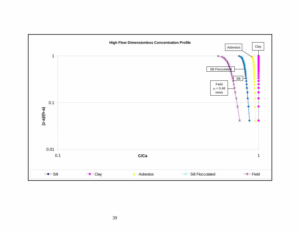
In the San Luis Canal, dimensionless concentration profiles were calculated for

different size fractions under different flow conditions. The concentration profiles for high flow are fairly uniform with near-surface concentrations at least 60% of the near-bed concentrations. At low flow, the San Luis Canal between Highway 198 and Jayne Avenue traps about 85% of the incoming sediment. At high flows, however, only about only about 30% of the sediment will be trapped, and except for sands, all size fractions are fairly well mixed over the vertical. Daily bedload and total load calculations show that the canal has the ability to transport about 10 cubic yards of sediment at low flow. At a high flow, the daily sediment load will be about 100 cubic yards for bedload and 10,000 cubic yards of total load.

Two main conclusions pertaining to the project can be made. First, the West Side Detention Basins are adequately designed. Second, at high flows in the San Luis Canal, all fractions but sand will be well mixed over the vertical. This allows for a direct diversion of water and sediment to Westlake Farms during flodds. The possibility of using near-surface sluices near Check 21 is considered feasibile and bottom sluices are not necessary when operating the canal at high discharges. At low flow, such sediment diversions would not be possible because the canal would act as a sediment trap.

29

REFERENCES Arroyo Pasajero Feasibility Study Appendix: Water Quality Report. Fifth Draft. June 2,

1997. Coleman, R.G. New Idria serpentinite a land management dilemma. Stanford University.

September 1995. Faria, Jose I. Sediment Transport Characteristics, Arroyo Pasajero and Tributaries

February and March 1991. State of California Department of Water Resources, August 1992.

http://wwwswpao.water.ca.gov/publications/bulletin/95/view/text/cha12.htm http://wwwswpao.water.ca.gov/publications/bulletin/96/text/cha6.html http://wwwswpao.water.ca.gov/publications/bulletin/96/text/cha12.html http://www.omwq.water.ca.gov http://www.smico.com/pdf/mat_density_grav_angle.pdf http://www.water.ca.gov/swp/facilities/water http://www.water.ca.gov/swp/history.html Julien, Pierre Y. Erosion and Sedimentation. Cambridge University Press, 1998. Leclerc, Rene F, Robert C. MacArthur, and Victor J. Galay. Arroyo Incision Due to

Tectonism and Land Subsidence, Arroyo Pasajero, California, 1997. Northwest Hydraulic Consultants. Geology of the Arroyo Pasajero Watershed. Water Quality Assessment of the State Water Project, 1994-1995. California Department

of Water Resources, Division of Operations and Maintenance, Water Quality Section. June 1997.

30

LIST OF PARAMETERS A = area of the channel a = depth from channel bed C = sediment concentration Ca = concentration at a given depth, a Cw = concentration by weight of sediment d* = dimensionless grain size ds = grain size f = Darcy Weisbach friction factor Fr = Froude number g = gravitational acceleration G = specific gravity h = water depth Q = flow rate of the channel qbv = bed material in motion per unit width Rh = hydraulic radius Ro = Rouse number Sf = friction slope TE = trap efficiency u* = shear velocity V = velocity vx = velocity in the x-direction x = distance along the channel X = distance downstream where a given particle will settle z = depth at a given location relative to the channel bed β = ratio of turbulent mixing coefficient to momentum exchange coefficient κ = von Karman constant νm = kinematic viscosity τ* = shields parameter ω = fall velocity ωf = flocculated fall velocity

31

Appendix A – Flocculation Testing

32

Water samples were collected while visiting the San Luis Canal and Arroyo Pasajero on June 13, 2003. San Luis Canal water was withdrawn directly from the canal. Arroyo Pasajero water was a little more difficult because of the season in which the site visit took place. There is a natural, flowing spring located on Los Gatos Creek that was used to collect a water sample for Arroyo Pasajero. There is some water quality information available for the San Luis Canal water; however, nothing was available for Arroyo Pasajero. The water quality information can be seen in the table below.

Temperature 21.4 ºCElectrical Conductivity 306 µS/cm

Turbidity 14.7 NTU With the collected water samples, a flocculation test was completed for the San Luis Canal water. There were three bottles all with about the same amount of sediment. About 35 g/l of table salt was added to the first bottle, the second bottle was left alone, and the third had a combination of 35.7 g/l of sodium hexametaphosphate and 7.9 g/l of sodium carbonate (deflocculant). All three bottles were mixed and placed next to each other. By looking at the three bottles side by side, it was possible to determine whether the sediment was flocculated. If the sediment were flocculated, then you would expect the sediment in both the bottle with salt and the bottle with no chemicals to settle before the sediment with the sodium hexametaphosphate and sodium carbonate. After experimentation, the plain bottle settled first, followed by the bottle with salt, and finally the bottle with the deflocculant, proving that the sediment flocculates. It took about seven minutes for the sediment to settle 20 centimeters, giving a fall velocity of 0.476 mm/s. There is one important conclusion that can be drawn from these results. During dry years where there is no natural mixing in the delta it is expected that there will be a greater amount of salt present in the water. This salt, as the experiment proves, will cause more sediment to be in suspension then on years where there is natural mixing in the delta. Pictures demonstrating this for both Arroyo Pasajero and the San Luis Canal can be seen below.

Arroyo Pasajero

AP

SaltDeflocculant

33

San Luis Canal

For the water samples collected in a tributary of Arroyo Pasajero, the full flocculation test was not completed. It was assumed that the sediment would again behave as a flocculated mass. A fall velocity was calculated in a manner similar to the San Luis Canal. It took 17 minutes for the sediment to fall 20 centimeters, giving a fall velocity of 0.196 mm/s. Both the San Luis Canal and the Arroyo Pasajero fall velocities were used in the calculations to represent flocculated clay. Using the same water samples, with only sediment and no chemicals placed in it, another test was conducted. The bottles were filled with about 40 percent sediment and 60 percent water. Once all the sediment had settled in each bottle, a line was drawn on the bottle representing the location of 100 percent settling. Lines between 0 and 100 were drawn on each bottle. At the same time, both bottles were mixed and then allowed to start settling. Once the sediment had settled to each line on the bottle, the time was recorded. Upon completion of the test, the results were plotted on a graph. The graph, referred to as Oden Curves, for both the San Luis Canal and Arroyo Pasajero follow.

SLC SaltDeflocculant

34

Oden Curve0

102030405060708090

1001E-02 1E+00 1E+02 1E+04 1E+06

Time (min)

Perc

ent i

n Su

spen

sion

by

Wei

ght

0102030405060708090100

Perc

ent S

ettle

d by

W

eigh

t

San Luis Canal Arroyo Pasajero

The values corresponding to both of these graphs can be seen in the tables below.

San Luis Canal Arroyo PasajeroTime (min) % Settled % Suspended Time (min) % Settled % Suspended

0 0 100 0 0 1000.03 10 90 0.17 10 900.17 20 80 0.5 20 800.33 30 70 1 30 70

1 40 60 1.6 40 602 50 50 3 50 505 60 40 5.5 60 409 70 30 10 70 30

30 80 20 40 80 20210 90 10 240 90 10

108000 100 0 129600 100 0 Throughout the experiment, there were a number of pictures taken. The pictures, shown below, show the experiment initially and 2 hours. Also, shown below is a graph showing the sediment distribution corresponding to these settling velocities.

35

Sediment Gradation

0

0.1

0.2

0.3

0.4

0.5

0.6

0.7

0.8

0.9

1

0.010.1

Grain Size,ds

Perc

ent F

iner

SLC AP

Initially

SLC AP

36

After 2 hours

SLC AP

37

Appendix B –Sediment Concentration Profiles

37

Low Flow Dimensionless Concentration Profile

0.01

0.1

1

0.001 0.01 0.1 1

(z-a

)/(h-

a)

C/Ca

Silt Clay Asbestos Silt Flocculated Field

Fieldω = 0.48

mm/s

ClayAsbestos

Silt Flocculated

Silt

38

Intermediate Flow Dimensionless Concentration Profile

0.01

0.1

1

0.1 1

(z-a

)/(h-

a)

C/Ca

Silt Clay Asbestos Silt Flocculated Field

Fieldω = 0.48

mm/s

ClayAsbestos

Silt Flocculated

Silt

39

High Flow Dimensionless Concentration Profile

0.01

0.1

1

0.1 1

(z-a

)/(h-

a)

C/Ca

Silt Clay Asbestos Silt Flocculated Field

Fieldω = 0.48

mm/s

ClayAsbestos

Silt Flocculated

Silt