SEDIMENT ASSESSMENT OF HOTSPOT AREAS IN THE

DULUTH/SUPERIOR HARBOR

Submitted to

Callie Bolattino, Project OfficerGreat Lakes National Program OfficeU.S. Environmental Protection Agency

77 West Jackson BoulevardChicago, Illinois 60604-3590

by

Judy L. Crane and Mary Schubauer-BeriganMinnesota Pollution Control Agency

Water Quality Division520 Lafayette Road North

St. Paul, Minnesota 55155-4194

and

Kurt SchmudeUniversity of Wisconsin

Lake Superior Research Institute1800 Grand Avenue

Superior, Wisconsin 54880

ii

DISCLAIMER

The information in this document has been funded by the U.S. Environmental Protection Agency’s(EPA) Great Lakes National Program Office. It has been subject to the Agency’s peer andadministrative review, and it has been approved for publication as an EPA document. Mention oftrade names or commercial products does not constitute endorsement or recommendation for use bythe U.S. Environmental Protection Agency.

iii

TABLE OF CONTENTS

Disclaimer ....................................................................................................................................... iiList of Figures ................................................................................................................................ viList of Tables.................................................................................................................................viiAcknowledgments .......................................................................................................................... ixList of Acronyms and Abbreviations .............................................................................................. x

1.0 Introduction ............................................................................................................................... 11.1 Background ................................................................................................................... 11.2 Project Description........................................................................................................ 21.3 Project Objectives ......................................................................................................... 31.4 Project Tasks ................................................................................................................. 4

2.0 Methods..................................................................................................................................... 52.1 Field Methods................................................................................................................ 5

2.1.1 Reconnaissance Survey and Site Selection ....................................................... 52.1.2 Sediment Collection .......................................................................................... 5

2.1.2.1 Sampling with a small MPCA boat....................................................... 52.1.2.2 Sampling with the R/V Mudpuppy ....................................................... 6

2.2 Sample Tracking ........................................................................................................... 82.3 Laboratory Methods ...................................................................................................... 9

2.3.1 Chemical Analyses ............................................................................................ 92.3.2 Sediment Toxicity Tests.................................................................................... 92.3.3 Benthological Community Structure................................................................. 9

2.3.3.1 Sample processing................................................................................. 92.3.3.2 Enumeration of benthic invertebrates.................................................. 102.3.3.3 Quality control..................................................................................... 112.3.3.4 Calculations......................................................................................... 11

3.0 Results ........... ......................................................................................................................... 123.1 Site Information........................................................................................................... 12

3.1.1 Sample Locations ............................................................................................ 123.1.2 Site and Sediment Descriptions....................................................................... 12

3.1.2.1 Bay south of the DM&IR taconite storage facility.............................. 123.1.2.2 Bay east of Erie Pier ............................................................................ 123.1.2.3 Howard’s Bay...................................................................................... 12

iv

TABLE OF CONTENTS (continued)

3.1.2.4 Kimball’s Bay...................................................................................... 133.1.2.5 Bays north and south of the M.L. Hibbard/DSD No. 2 plant .............. 133.1.2.6 Minnesota Slip .................................................................................... 143.1.2.7 City of Superior WWTP...................................................................... 143.1.2.8 Slip C................................................................................................... 153.1.2.9 WLSSD and Miller and Coffee Creek Embayment ............................ 15

3.2 Chemical Analyses ...................................................................................................... 163.2.1 Particle Size..................................................................................................... 173.2.2 Total Organic Carbon...................................................................................... 183.2.3 Ammonia......................................................................................................... 183.2.4 Total Arsenic and Lead ................................................................................... 183.2.5 AVS and SEM................................................................................................. 193.2.6 Mercury ........................................................................................................... 193.2.7 Dioxins/Furans ................................................................................................ 203.2.8 PAHs ............................................................................................................... 20

3.2.8.1 PAH fluorescence screen..................................................................... 203.2.8.2 PAHs by GC/MS................................................................................. 21

3.2.9 PCBs................................................................................................................ 223.2.9.1 Total PCBs .......................................................................................... 223.2.9.2 Congener PCBs ................................................................................... 22

3.3 Toxicity Tests .............................................................................................................. 233.3.1 Acute Toxicity to Hyalella azteca................................................................... 233.3.2 Acute Toxicity to Chironomus tentans ........................................................... 243.3.3 Chronic Toxicity to Chironomus tentans ........................................................ 24

3.4 Benthological Assessments ......................................................................................... 243.4.1 Sampling Design ............................................................................................. 243.4.2 Ecology and Feeding Habits of Abundant Benthic Organisms....................... 25

3.4.2.1 Oligochaetes: Naididae and Tubificidae ............................................ 253.4.2.2 Polychaetes: Manayunkia speciosa .................................................... 253.4.2.3 Phantom midges: Chaoborus.............................................................. 263.4.2.4 True midges: Chironomus.................................................................. 26

3.4.3 Site Assessments ............................................................................................. 263.4.3.1 DMIR sites .......................................................................................... 263.4.3.2 ERP sites ............................................................................................. 273.4.3.3 HOB sites ............................................................................................ 273.4.3.4 KMB sites............................................................................................ 27

v

TABLE OF CONTENTS (continued)

3.4.3.5 MLH sites ............................................................................................ 283.4.3.6 MNS sites ............................................................................................ 283.4.3.7 STP sites.............................................................................................. 283.4.3.8 SUS sites ............................................................................................. 283.4.3.9 WLS sites ............................................................................................ 29

3.4.4 Chironomid Deformities ................................................................................. 293.4.5 Quality Assurance/Quality Control ................................................................. 29

4.0 Sediment Quality Triad Approach .......................................................................................... 304.1 Background ................................................................................................................. 304.2 Application of the Triad Approach to the Duluth/Superior Harbor ............................ 314.3 Other Applications of the 1994 Data Set .................................................................... 324.4 Development of Hotspot Management Plans.............................................................. 34

5.0 Recommendations ................................................................................................................... 35

References ........... ......................................................................................................................... 38

Appendix A Sediment Chemistry DataAppendix B Sediment Toxicity Test Reports for Hyalella azteca and Chironomus tentansAppendix C Benthological Community Data

vi

LIST OF FIGURES

Figure 1-1. Total relative contamination factors (RCFs) for surficial sediments(i.e., 0-30 cm) collected during the 1993 sediment survey of theDuluth/Superior Harbor................................................................................... 41

Figure 2-1. Location of study sites..................................................................................... 42Figure 3-1. Map of DMIR sample sites ............................................................................. 43Figure 3-2. Map of ERP sample sites ................................................................................ 44Figure 3-3. Map of HOB sample sites ............................................................................... 45Figure 3-4. Map of KMB sample sites............................................................................... 46Figure 3-5. Map of MLH sample sites ............................................................................... 47Figure 3-6. Map of MNS sample sites ............................................................................... 48Figure 3-7. Map of STP sample sites................................................................................. 49Figure 3-8. Map of SUS sample sites ................................................................................ 50Figure 3-9. Map of WLS sample sites ............................................................................... 51Figure 3-10. Total lead depth profiles for Howard’s Bay.................................................... 52Figure 3-11. SEM/AVS depth profiles for three Howard’s Bay sites.................................. 53Figure 3-12. Mercury depth profiles for three WLSSD sites ............................................... 54Figure 3-13. Depth profile of mercury at Slip C.................................................................. 55Figure 3-14. Depth profile of screening PAHs at Slip C ..................................................... 56Figure 3-15. Depth profile of total PAHs (by GC/MS) at Slip C ........................................ 57Figure 3-16. Depth profile of normalized PAHs (by GC/MS) at Minnesota Slip ............... 58Figure 3-17. Depth profile of normalized PCB concentrations (ng/g oc) at the

Slip C sites....................................................................................................... 59Figure 3-18. Diagrams of: a) Tubificidae, b) Manayunkia speciosa, c) Chaoborus, and

d) Chironomus................................................................................................. 60

vii

LIST OF TABLES

Table 2-1. Sectioning Scheme for Chemical Analyses Performed at each Site ..................... 62Table 2-2. Summary of Sediment Analytical Methods .......................................................... 64Table 3-1. Site Coordinates for the 1994 Sediment Survey ................................................... 65Table 3-2. Description of Field Results for DM&IR, Erie Pier, and Kimball’s Bay

Areas (DMIR 1-4, ERP 1-5, and KMB 1-5) ......................................................... 67Table 3-3. Description of Field Results for Howard’s Bay (HOB 1-15)................................ 68Table 3-4. Description of Field Results for M.L. Hibbard/DSD No. 2 Plant and

Grassy Point Embayment (MLH 1-10) ................................................................. 70Table 3-5. Description of Field Results for Minnesota Slip (MNS 1-5) ................................ 71Table 3-6. Description of Field Results for City of Superior WWTP Embayment

(STP 1-8, STP 10, STP 12) ................................................................................... 72Table 3-7. Description of Field Results for Slip C (SUS 1-8)................................................ 74Table 3-8. Description of Field Results for WLSSD and Miller/Coffee Creek Embayment

(WLS 1-20) ........................................................................................................... 76Table 3-9. Particle Size Distribution of all Sample Sites and Depth Profiles ........................ 80Table 3-10. TOC Results for all Sample Sites and Depth Profiles........................................... 86Table 3-11. Ammonia Results for Selected Sites and Depth Profiles ...................................... 93Table 3-12. Total Arsenic and Lead Results for Howard’s Bay Samples ................................ 95Table 3-13. AVS Results for Selected Sites ............................................................................. 96Table 3-14. SEM Results for Selected Sites............................................................................. 99Table 3-15. SEM/AVS Ratios for Selected Sites ................................................................... 101Table 3-16. Comparison of SEM Lead and Total Lead Concentrations in Howard’s Bay .... 104Table 3-17. Mercury Results for Selected Sites and Depth Profiles....................................... 105Table 3-18. TCDD and TCDF Results for WLS and KMB Samples..................................... 109Table 3-19. Screening PAH Results for Selected Sites .......................................................... 111Table 3-20. PAH Results (by GC/MS) for Selected Sites ...................................................... 114Table 3-21. TOC-Normalized PAH Results for Selected Sites.............................................. 120Table 3-22. Total PCB Results for Selected Sites .................................................................. 125Table 3-23. Subset of Seven PCB Congeners ........................................................................ 130Table 3-24. Results for Seven PCB Congeners at Selected Sites........................................... 131Table 3-25. Mean Survival (%) of H. azteca and C. tentans Exposed to Test Sediments ..... 136Table 3-26. Normalized Survival (%) of H. azteca and C. tentans Exposed to

Test Sediments .................................................................................................... 137Table 3-27. Mean Total Abundance (individuals/m2) and Taxa Richness Values for the

Benthological Community Survey ...................................................................... 138

viii

LIST OF TABLES (continued)

Table 3-28. Mean Densities (number/m2), with Sample Standard Deviations inParentheses, and Percent Composition of each Macroinvertebrate Groupfor the DMIR Sites (n=3) .................................................................................... 142

Table 3-29. Mean Densities (number/m2), with Sample Standard Deviations inParentheses, and Percent Composition of each Macroinvertebrate Groupfor the ERP Sites (n=3) ....................................................................................... 143

Table 3-30. Mean Densities (number/m2), with Sample Standard Deviations inParentheses, and Percent Composition of each Macroinvertebrate Groupfor the HOB Sites (n=3) ...................................................................................... 144

Table 3-31. Mean Densities (number/m2), with Sample Standard Deviations inParentheses, and Percent Composition of each Macroinvertebrate Groupfor the KMB Sites (n=3)...................................................................................... 146

Table 3-32. Mean Densities (number/m2), with Sample Standard Deviations inParentheses, and Percent Composition of each Macroinvertebrate Groupfor the MLH Sites (n=3)...................................................................................... 147

Table 3-33. Mean Densities (number/m2), with Sample Standard Deviations inParentheses, and Percent Composition of each Macroinvertebrate Groupfor the MNS Sites (n=3) ...................................................................................... 148

Table 3-34. Mean Densities (number/m2), with Sample Standard Deviations inParentheses, and Percent Composition of each Macroinvertebrate Groupfor the STP Sites (n=3)........................................................................................ 149

Table 3-35. Mean Densities (number/m2), with Sample Standard Deviations inParentheses, and Percent Composition of each Macroinvertebrate Groupfor the SUS Sites (n=3 for SUS 1-7; n=1 for SUS 8).......................................... 150

Table 3-36. Mean Densities (number/m2), with Sample Standard Deviations inParentheses, and Percent Composition of each Macroinvertebrate Groupfor the WLS Sites (n=3) ...................................................................................... 151

Table 3-37. Number of Chironomid Larvae with Menta Deformities.................................... 153Table 4-1. Triad Analysis Endpoints for Sediment Quality in the Duluth/Superior

Harbor.................................................................................................................. 154Table 4-2. Number of Surficial Sites Sampled for each Component of the Sediment

Quality Triad ....................................................................................................... 155

ix

ACKNOWLEDGMENTS

This report was prepared by Judy Crane, Minnesota Pollution Control Agency (MPCA), withassistance from Mary Schubauer-Berigan, formerly of the MPCA, and Kurt Schmude, University ofWisconsin (UW)--Lake Superior Research Institute.

The study design and quality assurance project plan were developed by Mary Schubauer-Berigan.Field sampling was coordinated by Mary Schubauer-Berigan with assistance from MPCA,Wisconsin Department of Natural Resources (DNR), and Great Lakes National Program Office(GLNPO) personnel. Kurt Schmude, and other personnel from the UW-Lake Superior ResearchInstitute, collected and processed sediment samples for enumeration of the benthologicalcommunity. GLNPO’s research vessel (R/V), the Mudpuppy, and vibracorer device were used forthe collection of sediment samples.

Sediment toxicity tests were conducted by the MPCA Toxics Unit which included Carol Hubbard,Harold Wiegner, Patti King, Jerry Flom, and Scot Beebe. Chemical analyses were performed by thefollowing analytical laboratories: mercury - Wisconsin State Laboratory of Hygiene; PAHs (byGC/MS) - Huntingdon Engineering and Environmental, Inc.; dioxins, furans, PCBs, and particlesize - Trace Organic Analytical Laboratory, Natural Resources Research Institute (NRRI); and PAHscreen, AVS, SEM, ammonia, TOC, total lead, and arsenic - Central Analytical Laboratory, NRRI.

Excel spreadsheet support was provided by Scot Beebe, James Beaumaster, Jeff Canfield, and JanetRosen. Graphical support was provided by James Beaumaster. Word processing support wasprovided by Jennifer Holstad, Janet Eckart, and Janet Rosen.

This project was funded by the U.S. Environmental Protection Agency (EPA) GLNPO through grantnumber GL995636. Rick Fox and Callie Bolattino provided valuable input as the successiveGLNPO Project Officers of this investigation.

x

LIST OF ACRONYMS AND ABBREVIATIONS

AAS Atomic Absorption SpectroscopyAgNO3 Silver NitrateAOC Area of ConcernAR Analytical ReplicateAs ArsenicASTM American Society of Testing and MaterialsAVS Acid Volatile SulfideCd Cadmiumcm CentimeterCMD Classical Multi-dimensional ScalingCo CompanyCu CopperCV Coefficient of VariationDM&IR Duluth, Masabe, and Iron RangeDMIR DM&IR StockpileDSD Duluth Steam DistrictEPA Environmental Protection AgencyER Extraction ReplicateERP Erie PierFe Ironft FeetGC/ECD Gas Chromatography/Electron Capture DetectionGC/MS Gas Chromatography/Mass SpectrometryGIS Geographic Information SystemGLNPO Great Lakes National Program OfficeGPS Global Positioning SystemHg MercuryHOB Howard’s BayIJC International Joint CommissionKCl Potassium Chloridekg KilogramKMB Kimball’s BayLEL Lowest Effect LevelLOD Limit of DetectionLOQ Limit of QuantitationLSRI Lake Superior Research Institutem Metermg MilligramMLH M.L. Hibbard/DSD No. 2 and Grassy Point areamm MillimeterMN Minnesota

xi

LIST OF ACRONYMS AND ABBREVIATIONS (continued)

MNS Minnesota SlipMPCA Minnesota Pollution Control AgencyN NorthN/A Not ApplicableND Not DetectedNEL No Effect LevelNH3 AmmoniaNi NickelNRRI Natural Resources Research InstituteNOAA National Oceanographic and Atmospheric AdministrationNQ Not QuantifiableOC Organic CarbonOMOEE Ontario Ministry of Environment and EnergyPAH Polycyclic Aromatic HydrocarbonPb LeadPCB Polychlorinated BiphenylPDOP Position Dilution of PrecisionPPDC Post Process Differential CorrectionQA/QC Quality Assurance/Quality ControlQAPP Quality Assurance Project PlanQC Quality ControlRAP Remedial Action PlanRCF Relative Contamination FactorR-EMAP Regional Environmental Monitoring and Assessment ProgramRI/FS Remedial Investigation/Feasibility StudyRPD Relative Percent DifferenceRSD Relative Standard DeviationRTR Ratio-to-Reference ValueR/V Research VesselSA Selective AvailabilitySD Standard DeviationSEL Severe Effect LevelSEM Simultaneously Extractable MetalsSOP Standard Operating ProcedureSQG Sediment Quality GuidelineSTP Sewage Treatment PlantSUS Slip CTCDD Tetrachlorodibenzo-p-dioxin (as in 2,3,7,8-TCDD)TCDF Tetrachlorodibenzofuran (as in 2,3,7,8-TCDF)TOC Total Organic Carbon

xii

LIST OF ACRONYMS AND ABBREVIATIONS (continued)

µg MicrogramUMD University of Minnesota-DuluthUWS University of Wisconsin-SuperiorVC VibrocorerW WestWDNR Wisconsin Department of Natural ResourcesWI WisconsinWLS WLSSD/Coffee and Miller Creek BayWLSSD Western Lake Superior Sanitary Districtwt. WeightWWTP Wastewater Treatment PlantZn Zinc

1

CHAPTER 1

INTRODUCTION

1.1 BACKGROUND

The St. Louis River and the Duluth/Superior Harbor consist of a variety of habitat types, rangingin character from relatively pristine streams and wetlands to an industrialized harbor containingtwo Superfund sites. Many current and former dischargers have contributed to the contaminationof sediments within this Area of Concern (AOC). Currently, there are only a few permitted pointsource discharges to the waters of the AOC. These include (in Minnesota): the Western LakeSuperior Sanitary District (WLSSD), which collects and treats both municipal and industrialwastes for the entire region of the AOC from Cloquet to Duluth. In Wisconsin, current majorNPDES dischargers to the waters of the AOC include the Superior Municipal WastewaterTreatment Plant (WWTP), Murphy Oil-Superior Refinery, and Superior Fiber Products (whosewastewater is transported to WLSSD for treatment).

The geological setting, anthropological history, and recent environmental knowledge about theAOC are documented in the Stage I Remedial Action Plan (RAP) document [MinnesotaPollution Control Agency (MPCA)/Wisconsin Department of Natural Resources (WDNR),1992]. During the past five years, the MPCA and its collaborators have been actively involved indelineating the extent of sediment contamination in the St. Louis River AOC. These studiesinclude:

• Preliminary assessment of contaminated sediments and fish in the Thomson, Forbay, andFond du Lac Reservoirs (Schubauer-Berigan and Crane, 1996)

• Survey of sediment quality in the Duluth/Superior Harbor: 1993 sampling results

(Schubauer-Berigan and Crane, 1997) • Sediment assessment of hotspot areas in the Duluth/Superior Harbor (this report) • Regional Environmental Monitoring and Assessment Program (R-EMAP) surveying,

sampling, and testing: 1995 and 1996 sampling results [draft report in process of beingprepared by the MPCA, Natural Resources Research Institute (NRRI), and U.S.Environmental Protection Agency (EPA)]

• Sediment remediation scoping project at Slip C in the Duluth Harbor (report to be prepared

by the MPCA during the spring of 1998)

2

• Development of sediment quality guidelines for the St. Louis River AOC (new project begunOctober 1, 1997)

• Bioaccumulation of contaminants in the Duluth/Superior Harbor (new project begun October 1, 1997).

The above investigations have been, or are being, conducted with the cooperation and financialsupport of the U.S. EPA. These studies will support the assessment and hotspot managementplan goals of the Phase I sediment strategy for the RAP. The chemistry data from most of theseinvestigations are being entered into two similar, but separate, geographic information system(GIS)-based databases for the Duluth/Superior Harbor. The databases are maintained by the U.S.Army Corps of Engineers and EPA’s Great Lakes National Program Office (GLNPO).

In this report, the results of the 1994 sediment assessment of hotspot areas in the Duluth/SuperiorHarbor will be presented. Due to the large number of figures and tables in this report, all of themhave been moved to the end of this report.

1.2 PROJECT DESCRIPTION

A general assessment of sediment contamination in the Duluth/Superior Harbor was conductedduring 1993. The results of this MPCA investigation indicated that polycyclic aromatichydrocarbon (PAH) contamination was widespread throughout the harbor (Schubauer-Beriganand Crane, 1997). Heavy metal, mercury, selected pesticide, and polychlorinated biphenyl (PCB)contamination was also of concern at several sites. The Duluth portion of the harbor wasgenerally more contaminated than the Superior portion of the harbor (Figure 1-1).

The USX Superfund site was the most contaminated site evaluated in the 1993 sediment survey(Schubauer-Berigan and Crane, 1997). This site, along with the Interlake/Duluth Tar Superfundsite, have been undergoing additional investigations as part of the potentially responsible partieslegal obligations. Other sites that were rated highly for further study included: Hog Island Inletand Newton Creek, the bay surrounding WLSSD and Coffee/Miller Creek outfalls, FraserShipyards, Minnesota Slip, area between the M.L. Hibbard Plant/Duluth Steam District (DSD)No. 2 and Grassy Point, and in the old 21st Ave. West Channel. Other areas, such as Slip C andoff the city of Superior wastewater treatment plant (WWTP) outfall, were listed as mediumpriority. It is important to note that this 1993 study was limited in scope and was not meant tocharacterize large areas as to the extent of contamination.

The results of the 1993 sediment survey were used to shape the scope of this project. TheMPCA, in cooperation with GLNPO and WDNR, conducted a sediment survey of the followinghotspot areas during the fall of 1994:

• Bay south of the DM&IR taconite storage facility

3

• Bay east of Erie Pier• Howard’s Bay (including Fraser Shipyards)• Area north of Grassy Point and in the vicinity of M.L. Hibbard/DSD No. 2• Minnesota Slip• City of Superior WWTP• Slip C• WLSSD, Miller Creek, and Coffee Creek Embayment• Kimball’s Bay (reference site).

The two Superfund sites and the Hog Island Inlet/Newton Creek sites were not included in thisstudy due to other in-depth investigations that were already underway at these sites. Two sitesthat were ranked low priority for further study in the 1993 sediment investigation were includedin this survey. Erie Pier was included because of acute sediment toxicity that was observed at the1993 sample site. DM&IR was included to confirm the 1993 observation that this site was notvery contaminated.

A sediment quality triad approach (Long and Chapman, 1985) was used in this study tocharacterize sediment quality at each site. Synoptic measures of sediment chemistry, sedimenttoxicity, and benthological community structure were made at selected sites. A short-list ofcontaminants was measured in various core sections based on the results of the 1993 sedimentsurvey. Ten-day sediment toxicity tests, using Hyalella azteca (H. azteca) and Chironomustentans (C. tentans), were used to assess biological effects under controlled conditions. Thebenthological community structure was used to assess in situ biological effects. Sediments thatdemonstrated a high degree of concordance among all three measures were considered to havedegraded sediment quality and pose a risk to the environment. Sediments that showedconcordance between two of the three measures may or may not be degraded and warrant furtherinvestigation.

1.3 PROJECT OBJECTIVES

The primary objectives of this investigation were to:

• Perform site-specific assessments of sediment contamination, toxicity, and benthiccommunity structure at areas identified during the 1993 sediment survey as having elevatedcontamination. A similar Triad assessment was performed at a reference site (i.e., Kimball’sBay).

• Develop a sediment management plan for study sites where the presence of contaminants are

associated with toxicity and/or impaired benthic communities.

4

1.4 PROJECT TASKS

Specific project tasks included the following:

• Measure concentrations of selected contaminants at eight contaminated sites, and onereference site, in the Duluth/Superior Harbor. Contaminants of concern included: PCBs,PAHs, PAH screen, TCDD and TCDF, mercury, lead, arsenic, simultaneously extractablemetals (SEM) (i.e., cadmium, copper, nickel, lead, and zinc), and ammonia. In addition, totalorganic carbon (TOC), acid volatile sulfide (AVS), and particle size were measured.

• Perform sediment toxicity tests with H. azteca (10-day survival) and C. tentans (10-day

survival and growth) at half of the locations within each site (selected on a worst-case basis)using EPA-developed methodologies.

• Conduct a benthic community assessment at each site by sampling macrobenthos at all of the

locations within each site, identifying organisms to the lowest possible classification, andusing community evaluation metrics to determine the ecological status of the benthiccommunity.

• Use the sediment quality triad approach to integrate chemistry, toxicity, and benthiccommunity assessment data.

• Develop sediment management plans for areas with contaminated sediments in theDuluth/Superior Harbor.

5

CHAPTER 2

METHODS

2.1 FIELD METHODS

2.1.1 Reconnaissance Survey and Site Selection

The sites examined in this study were located in the St. Louis River and Duluth/Superior Harbor,downstream of the Kimball's Bay area (Figure 2-1). General site selection resulted from analysisof the data from the 1993 Duluth/Superior Harbor sediment survey (Schubauer-Berigan and Crane,1997). Contaminated sites were also selected in consultation with WDNR and GLNPO sedimentpersonnel. The area of Kimball's Bay was selected as a “clean” reference site for the eight hotspotareas in the Duluth/Superior Harbor.

A stratified random sampling approach was used for final site selection within each of the nineareas. Sampling locations were obtained by placing a grid (of a size appropriate to generate thedesired number of samples at each site) over the site map. The grid size was determined by thesize of the area to be sampled, as well as the complexity of contaminant sources or hydrodynamicsof the site. For example, at the WLSSD and Miller and Coffee Creek embayment site, a grid sizeof 150 m was used to more finely distinguish the three contaminant sources. A larger grid size of400 m was used at the M.L. Hibbard/DSD No. 2 and Grassy Point area to bracket contaminationover a wider area.

During July and August of 1994, several locations to be sampled intensively duringSeptember 1994 were scoped out during reconnaissance surveys. Specifically, locations in theWLSSD and Miller/Coffee Creek embayment, the area in Howard's Bay near Fraser Shipyards,and the bay near Barker’s Island and the City of Superior WWTP were surveyed with theassistance of the WDNR survey team. In these reconnaissance surveys, the pre-selected gridpoints were evaluated for the suitability of the substrate for surficial sediment sampling. Thegeographical coordinates were surveyed by the WDNR team, and the global positioning system(GPS) coordinates were recorded by MPCA staff. All sample coordinates were recorded with aTrimble Pathfinder Basic Plus GPS. These GPS coordinates were used to revisit the sites duringthe actual sampling in September 1994; however, the final (official) sampling coordinates arethose recorded in the field during sampling.

2.1.2 Sediment Collection

2.1.2.1 Sampling with a small MPCA boat

The bays north and south of the M.L. Hibbard/DSD No. 2 plant (MLH sites), as well as the baysouth of the DM&IR taconite storage facility (DMIR sites), were sampled prior to Kimball’s Bayand the other sites in the Duluth/Superior Harbor. A small MPCA vessel was used for the field

6

sampling. This was necessitated by the shallow water depths at these sites (i.e., 1-3 m) and/ordifficulty of access (caused by anchored wood debris) experienced by the R/V Mudpuppy duringthe 1993 survey. The ten sites in the M.L. Hibbard Plant/DSD No. 2 and Grassy Point bays, andfive sites in the DM&IR bay, were sampled during August 22-24, 1994. At each of the tenlocations in the Hibbard Plant/Grassy Point bays, geographical coordinates were ascertained usinga GPS unit. At each site location, a minimum of 100 data points were collected with the GPS unitwhile tracking at least four satellites (3D mode) with a position dilution of precision (PDOP) valueof less than six. Recorded data were downloaded on a personal computer daily, and the errorcaused by selective availability (SA) was eliminated utilizing post process differential correction(PPDC). This process was carried out using Pfinder software version 2.54 and base files from theMinnesota Power Base Station in Duluth. These final coordinates were accurate to within 2-5 mand were used to construct site maps.

After positioning and anchoring the boat, two types of sediment core samples were collected at theMLH sites: several gravity cores, which collected the top 13.5-22 cm of sediment, and a single,long manually-driven core (collected with a Livingston corer), which collected sediment to thebottom of the soft penetrable layer (0.4-0.95 m). The shorter surficial (gravity) cores werecombined to provide sufficient material for analysis of selected contaminants (Table 2-1) andwhere indicated, toxicity tests. In addition, three individual gravity cores collected from eachlocation were sieved through a standard 40-mesh screen, and the residue was preserved in aformalin solution within 24 hours of collection for enumeration of the benthos. The water and softsediment depths were measured at each site using a sediment poling device similar to thatdeveloped by the WDNR sediment team.

The gravity core samples for chemistry and toxicity were decanted of their overlying water. Next,the samples were either placed directly into a precleaned sample jar (in the case of the chemistrysamples), or combined and homogenized in a large acid- and solvent-cleaned glass bowl wherethey were split into two, 1-L jars for toxicity testing. Each deep Livingston core was extruded onsite and visually described from the surface to maximum depth. The bottom 15-27 cm section ofthe core was then removed from the core and placed into a 1-L glass jar for later homogenizationand subsequent splitting for chemical analysis.

At the DM&IR taconite storage facility site, a Ponar sampler was used because of the presence oflarge amounts of taconite pellets. The pellets made the sediment too heavy to be collected with agravity corer. Only surficial samples were collected for toxicity, benthos, and contaminantanalysis. After collection with the Ponar sampler, the samples were treated similar to those fromthe MLH sites.

2.1.2.2 Sampling with the R/V Mudpuppy

The other sites were sampled during September 21 to October 3, 1994 using GLNPO’s researchvessel (R/V), the Mudpuppy. The R/V Mudpuppy is a monohull aluminum barge with an overalllength of 9.2 m, a 2.4 m beam, and a draft of 0.5 m (Smith and Rood, 1994). It is designed forcollecting deep cores, using a vibrocorer, in shallow areas. The sites were sampled in thefollowing order during the fall of 1994.

7

• WLSSD/Miller and Coffee Creek embayment (WLS 1-20): September 21, 23, 26-27• Slip C (SUS 1-8): September 22 and October 3• Howard's Bay (HOB 1-15): September 27-29• City of Superior WWTP (STP 1-12): September 29-30 and October 3• Minnesota Slip (MNS 1-5): September 30• Erie Pier embayment (ERP 1-5): October 4• Kimball's Bay (KMB 1-5): October 4.

The sampling protocols for core collection were the same for all sites within all locations, and aresummarized as follows. The predetermined geographical coordinates were used to guide the R/VMudpuppy to the sampling position. The GPS unit, rather than the boats Loran unit, was thedevice of record for locating the desired position. In all cases, positioning was confirmed bysighting the boats position with reference to visual landmarks. The R/V Mudpuppy was thentriple-anchored on-site, water depth measured, sampling start time noted, and the final positionrecorded on the GPS unit.

The R/V Mudpuppy was accompanied by a small boat operated by researchers from the Universityof Wisconsin-Superior (UWS); they processed the benthos samples. Small (i.e., 5 cm diameter)gravity cores were used for sampling benthos, toxicity, and surficial chemistry samples because oftheir non-disruptive nature and ability to obtain a relatively undisturbed sediment-water interface.The vibrocorer was used to sample sediments deeper than 15 cm where desired. Benthos sampleswere collected prior to the vibrocores at each site by deploying the gravity corer one to three timesper replicate (depending on the depth sampled at each general location). Three benthos samplereplicates were collected at each site. The benthos core replicates were sieved in the field using awash bucket (Wildco, Saginaw, MI) with a U.S. no. 40 mesh (425 m opening). The debrismaterial was placed in a glass sample jar, preserved with 10% formalin solution containing rosebengal stain, and labeled. Samples were brought to the Lake Superior Research Institute (LSRI)for storage and processing on a daily basis. The number of cores per replicate and sampled depthwere recorded in the study field notebook, along with a description of the sediment substrate.

After the collection of the benthos samples, several short gravity cores were obtained at each sitefor the surficial chemistry and toxicity samples. The number of cores collected varied by site;generally, cores were collected until sufficient volume was obtained to perform chemistry and/ortoxicity analyses (i.e., about 2.5 L). The number, depth, and physical description of cores thuscollected were recorded in the field notebook. The cores were decanted of overlying water andplaced directly into a precleaned 1-L jar (chemistry samples). The toxicity samples werecombined and homogenized in an acid- and solvent-cleaned glass mixing bowl and split into two1-L glass jars. All samples were immediately placed on ice. At the end of each day, the sampleswere transferred to a storage refrigerator at the MPCA’s Duluth Regional office.

Deeper core sections for chemical analyses were obtained using the vibrocorer on board the R/VMudpuppy. As in the 1993 sediment assessment project, a 3-m long core tube, lined with a 4-mmwall thickness butyrate core tube liner, was attached to the vibrocorer head. Cores were collectedaccording to the standard operating procedures (SOPs) detailed in the Quality Assurance Project

8

Plan (QAPP) (Schubauer-Berigan, 1994) and in Smith and Rood (1994). Cores were, in general,driven to the point of refusal at each site. Core displacement and measured length were recorded.A single vibrocore sample was collected at each site.

The vibrocore was processed on board the R/V Mudpuppy immediately after collection. Beforelifting anchor, the sample processing crew extruded the core on the boat deck. The core wassectioned by sawing off the top 15 cm of the core to provide the first (surficial) section. Thissection was discarded, because surficial sediment was analyzed using samples collected by thegravity corer. The core was then sectioned at succeeding 15 cm intervals. The sections retainedfor chemical analysis depended on the sampling goals, which varied from site-to-site. Table 2-1gives the sectioning scheme for cores collected at each of the nine areas. A 15-cm section lengthprovided sufficient sample volume (approximately 1.5 L) to perform all the analyses required foreach section.

The visual characteristics of the core sections were described in the field notebook. The coresection was then decontaminated by scraping away and discarding the outer 2-3 mm, using asolvent- and acid-cleaned Teflon® spatula. Individual core sections were placed into a 4-L acid-and solvent-rinsed glass container and homogenized by stirring. Homogenized core sections wereplaced into precleaned 1-L glass jars and left on ice while on board the R/V Mudpuppy. At theend of each day, the samples were delivered on ice to a storage refrigerator at the MPCA’s DuluthRegional Office.

2.2 SAMPLE TRACKING

The benthos samples were transported to LSRI on a daily basis during field sampling. After fieldsampling was completed, the toxicity test samples were brought directly to the MPCA ToxicologyLaboratory in St. Paul, MN where the tests were conducted. The samples were stored at 4° C in arefrigerator in a controlled access room. Within one month of field collection, most of therefrigerated core sections for chemical analysis were apportioned into precleaned jars by a MPCAtechnician and were delivered to the contract laboratory. The Wisconsin State Laboratory ofHygiene could not store all of the mercury samples. Thus, they requested batches of samples to besent to them over a period of several months. All samples for chemical analyses wereaccompanied by sample tracking forms, which tracked the sample conditions and handling byMPCA and contract personnel.

Formal chain-of-custody procedures were not followed since the sample data were not intended tobe used for enforcement purposes.

9

2.3 LABORATORY METHODS

Standard operating procedures (SOPs) for the chemical analyses, toxicity testing, and benthossampling are appended to the Quality Assurance Project Plan (QAPP) for this project (Schubauer-Berigan, 1994). The methods are cited in the following sections for reference purposes.

2.3.1 Chemical Analyses

A summary of the analytical procedures used in this investigation are given in the QAPP(Schubauer-Berigan, 1994) and in Table 2-2. A PAH fluorometric screening method was used toprovide a low-cost procedure for locating PAH-contaminated sediments. This method wascalibrated using PAH results determined by EPA Method 8270.

2.3.2 Sediment Toxicity Tests

Sediment toxicity tests were conducted to assess acute (survival) and chronic (growth) toxicity tobenthic invertebrates. Acute effects were measured in separate 10-day toxicity tests to Hyalellaazteca (H. azteca) and Chironomus tentans (C. tentans). Growth was measured at the end of theC. tentans test to assess chronic effects. Survival and growth endpoints were compared toorganisms similarly exposed to a reference control sediment collected from West Bearskin Lake(Cook County, MN).

The toxicity tests were conducted using the procedures described in U.S. EPA (1994a). The testorganisms (H. azteca and C. tentans) were exposed to sediment samples in a portable, mini-flowsystem described in Benoit et al. (1993) and U.S. EPA (1994a). The test apparatus consists of 300mL, glass-beaker test chambers held in a glass box supplied with water from an acrylic plasticheadbox. The beakers have two, 1.5 cm holes covered with stainless steel mesh, to allow for waterexchange, while containing the test organisms. The headbox has a pipette tip drain calibrated todeliver water at an average rate of 32.5 mL/min. The glass box is fitted with a self-starting siphonto provide exchange of overlying water. Overlying water for the tests was nonchlorinated wellwater. The overlying water was monitored daily for pH, dissolved oxygen, and temperature.

The Hyalella azteca and Chironomus tentans tests were required to meet quality assurance (QA)requirements such as acceptable control sediment survival (i.e., mean survival of 80% for H.azteca and 70% for C. tentans), and acceptable performance on reference toxicant tests (i.e., testresults within two standard deviations of the running mean). Reference toxicant tests were notperformed with C. tentans, because they do not survive well in water-only tests.

2.3.3 Benthological Community Structure

2.3.3.1 Sample processing

Sample tracking work sheets were created for all samples, and the date and initials of the personperforming the activity was entered for each step in the processing procedure. Samples wereinitially decanted to remove the formalin, and the debris was rinsed on a U.S. no. 40 mesh sieve

10

(i.e., 425 m opening). The debris was either picked immediately to remove all organisms, or itwas represerved with 70% ethanol for later processing. All organisms were systematically pickedfrom the debris by placing a spoonful of debris in a large gridded petri dish, placing the dish on alight table, and viewing it under low power (i.e., 7X magnification) through a dissectingmicroscope with additional overhead light. The entire sample was picked in this way. Theorganisms were placed in 1-dram vials and preserved in 70% ethanol for later identification andlong-term curation. The sample debris was placed into a properly labeled storage jar (i.e., 50 to120 mL) for later quality control checks and long-term storage.

2.3.3.2 Enumeration of benthic invertebrates

Organisms were separated into three groups: Chironomidae/Chaoboridae/Ceratopogonidae(midges), Oligochaeta (worms), and all other invertebrates. All of the "other invertebrates" wereidentified by the Senior Taxonomist, Dr. Kurt L. Schmude (UWS LSRI). Empty mollusc shellswere disregarded. Pieces of invertebrates were picked and counted if the piece was determined tohave come from a live organism at the time of collection and it did not belong to an existingspecimen. However, only pieces of oligochaetes with the anterior portion, showing the mouthopening, were mounted and identified; other pieces of oligochaetes were not counted.Invertebrates were identified to the following taxonomic levels:

• Bivalvia - genus• Gastropoda - family or species• Nematoda - nematodes• mites - mites• Oligochaeta - genus or species• Polychaeta - species• Turbellaria - turbellaria• Hirudinoidea - species• Diptera - genus, species group, or species• Trichoptera - genus• Ephemeroptera - genus or species.

Immature tubificid oligochaetes do not have well developed sexual structures, which are necessaryfor definitive identification of several species. Consequently, these individuals were separated intothree groups: 1) immature tubificids without dorsal hair chaetae; 2) immature tubificids withdorsal hair chaetae; and 3) very immature tubificids lacking all chaetae. Although specimens inthese three groups likely represent species with individuals already identified from the samereplicate, these groups were treated as separate taxa and were included in taxa richness counts.

All midges and worms were mounted on slides using Hoyer's mounting medium. One midge wasmounted per cover slip, and up to three cover slips were mounted per slide. Up to ten worms weremounted per cover slip, with one to two cover slips per slide. About 1,500 slides were prepared.An undergraduate biology student was trained by the Senior Taxonomist to assist in theidentification of midges and worms. However, all identifications were made or verified by the

11

Senior Taxonomist. Data for each sample were recorded on separate data sheets and arranged in athree-ringed binder according to site and station.

2.3.3.3 Quality control

The sample tracking work sheets were used to record the steps through which each sample went inthe sample processing and identification procedures. Quality control (QC) checks were performedon the picking procedure. One randomly chosen sample out of every ten samples was immediatelyrepicked for accuracy; a total of 25 samples were repicked by the Senior Taxonomist

2.3.3.4 Calculations

The core sampler had an inner diameter of 1.62 inches (or 4.13 cm). Thus, the total surface area ofbottom substrate collected per core was calculated as 13.4 cm2. The data were converted tonumbers of organisms per square meter by using the following conversion factors:

1 core per replicate = 747.42 cores per replicate = 373.73 cores per replicate = 249.1

The Ponar grab sampler was 6x6 inches, which was equivalent to 232.2 cm2 of surface area ofbottom substrate collected per grab. A conversion factor of 43.06 was used for Ponar samples.

12

CHAPTER 3

RESULTS

3.1 SITE INFORMATION

3.1.1 Sample Locations

Figure 2-1 shows the overall locations of the hotspot areas sampled in the Duluth/Superior Harbor.The Kimball’s Bay area was included as a reference site. The precise location of the coringstations within the nine general areas sampled are shown in Figures 3-1 through 3-9. Thegeographical coordinates of these stations are provided in Table 3-1.

3.1.2 Site and Sediment Descriptions

3.1.2.1 Bay south of the DM&IR taconite storage facility

Five sites were sampled in the bay south of the DM&IR taconite storage facility (DMIR 1-5;Figure 3-1). A small MPCA vessel was used to sample the sites on August 23, 1994. Because allthe sediments at these locations were a dark brown silty clay with a high concentration of taconitepellets, the gravity corer could not be used. Instead, a Ponar grab sampler was used to obtain thesurface sediments. A single Ponar was used per benthos replicate (Table 3-2).

3.1.2.2 Bay east of Erie Pier

The small bay east of Erie Pier and southwest of the International Welding and Machinists site wassampled for benthos enumeration, toxicity testing, and surficial chemistry analysis (Table 3-2).Five sites, ERP 1-5, were visited in this area (Figure 3-2) on October 4, 1994. Three cores perreplicate were used for benthos enumeration. Toxicity tests were conducted using surficialsediment from sites ERP 1, 2, and 3. The gravity corer obtained very short cores at this site (5-8cm in depth). The physical descriptions of the sediments obtained from these sites are provided inTable 3-2. The sediments were quite variable in this bay.

3.1.2.3 Howard's Bay

Fifteen sites were sampled within Howard's Bay (HOB 1-15) (Figure 3-3). Eight of these siteswere sampled for toxicity testing using a "worst-case" approach. Benthos and chemistry sampleswere taken for surficial sediments at all sites (Table 3-3). Two additional sediment sections, fromthe vibrocore, were submitted for chemical analyses (as described in Table 2-1).

The visual description of the Howard's Bay sediments is given in Table 3-3. Samples HOB 1, 2, 3,5, 7, and 11 were located in the shipping lane within Howard's Bay, with site HOB 1 being closestto the mouth of the bay and site HOB 15 closest to the end of the bay (Figure 3-3). Sites HOB 4,

13

6, and 10 were located north of the Howard's Bay shipping channel, and south of the Main St.(Superior) peninsula.

Sites HOB 8 and 9 were just outside the entrance to active Dry Dock No. 2. These sites seemedvery well-scoured. The substrate was extremely hard red clay (with a bit of grit overlying the clayat site HOB 9). Because this hardpan was nearly impossible to sample with the vibrocorer, deepcores were not taken at these two sites. The gravity corers were able to obtain only very shortcores at these two sites (5 cm deep). Due to the great water depth at this location (7.0 m), it wasnot possible to manually push the core deeper into the sediment as was done at the MLH sites.

Sites HOB 12 and 13 were located just outside the entrance to Dry Dock No. 1 (also active). Thegravity corers were able to penetrate a bit deeper into these sediments (10 cm); however, thesesites were also well-scoured, with the hardpan located very close to the surface. Therefore,vibrocore samples were not collected at these two sites.

Sites HOB 14 and 15 were located at the terminus of the bay, past the boundary of the dredgedchannel. Site 15 was sampled as far to the end of the bay as the Mudpuppy could venture. Thetwo sites were very different from one another. The surface sediment from HOB 14 was verysimilar to those sediments north of the shipping channel, consisting of a loose, flocculent sand/claymixture atop clay. The deep core was very stiff red and brown clay to the bottom (0.45 m). Thesurface sediment from site HOB 15 was very similar: dark brown loose clay with gritty sand. Incontrast, deep sediment from this site contained very heavy black oil, for the entire depth, from0.15-1.2 m. An oil slick was apparent on the water surface while sampling.

3.1.2.4 Kimball's Bay

An area of Kimball's Bay, just west of Billings Park, was used as a reference site based on theresults of the 1993 survey. Only surficial samples were obtained from these sites. Five sites weresampled (KMB 1-5) on October 4, 1994 (Figure 3-4). Sites KMB 1, 2, and 3 were located in thelarge, open area of Kimball's Bay, whereas sites KMB 4 and 5 were located in two smaller arms ofthe bay. Toxicity tests were conducted with sediment from sites KMB 4 and 5. Three gravitycores were collected per replicate for the benthos enumeration (Table 3-2).

Sediment descriptions of the sites are given in Table 3-2. Sediments from these sites weredescribed, in general, as soft brown clay with or without the presence of an oxidized iron layernear the top of the gravity core.

3.1.2.5 Bays north and south of the M.L. Hibbard/DSD No. 2 plant

Ten sites were sampled from the bays. Samples for toxicity tests were collected at sites MLH 1-6as a "worst-case" evaluation (Table 3-4). Sites MLH 1-4 were on the north side of the M. L.Hibbard/DSD No. 2 plant, and sites MLH 5-10 were in the bay south of the plant (Figure 3-5). Agravity corer was used to collect surficial sediments at most of the locations. However, at sitesMLH 2, 3, and 6 (which had less penetrable gritty fly ash), the corer was modified by duct-tapingit to a grappling hook in order to sample the appropriate layer (i.e., 0-15 cm). The sub-surfacesediments were sampled with a Livingston corer to obtain the deepest layer possible. Chemical

14

analyses were performed on two sections from each site: 0-15 cm and the deepest layer obtainable(Table 3-4).

3.1.2.6 Minnesota Slip

Five cores (MNS 1-5) were collected in Minnesota Slip, the northeastern-most slip in theDuluth/Superior Harbor, just inside the Duluth entry (Figure 3-6). Four core sections werecollected and analyzed for sediment chemistry at each site. Three gravity cores per replicate wereused for the benthos enumeration (Table 3-5).

Descriptions of the sediments obtained from Minnesota Slip are given in Table 3-5. Of all theareas sampled in this sediment assessment, the Minnesota Slip core sections showed the highestdegree of oil contamination.

3.1.2.7 City of Superior WWTP

The outfall of Superior's WWTP is on a small peninsula, adjacent to the dredged Superior FrontChannel. Two sites were sampled on the northwest side of the outfall, and eight in the bay to thesoutheast of the outfall and near Barker's Island (Figure 3-7). Toxicity test samples were collectedat sites closest to the outfall location: STP 1, 3, 4, 6, and 7. The sampling protocol called for threesediment sections to be analyzed from these sites: 0-15 cm (collected with the gravity corer), aswell as 15-30 cm and 30-45 cm (collected with the vibrocorer). A total of three vibrocorer nosecones were lost at sites STP 3 and STP 5; therefore, extreme care had to be taken not to penetratethe clay too deeply on subsequent sampling attempts.

Descriptions of the sediments sampled in this area are given in Table 3-6. Because of thedifficulty involved with coring some of the sediments, it was decided to drop site STP 11, alongthe Superior Front Channel. In addition, site STP 10, which was in the deeper portion of the bay,was very sandy in the surficial sediment layer. Attempts to find softer sediment in this area wereunsuccessful; therefore, it was decided not to vibrocore these sediments in order to prevent thepotential loss of another nose cone. Site STP 9 could not be sampled due to the shallow waterdepth. Sites STP 6-8 were located in the center of the bay. Again, because of concerns aboutlosing nose cones, the vibrocoring was limited to approximately the top 0.4 m to avoid the hardsand layer below.

From site STP 8, the water depth was not suitable for sampling until the area near site STP 10. Thefinal site in this bay, STP 12, was quite different from the other sites. The surficial sediment wassoft, loose brown clay, with a slight oil sheen. A deeper core was obtainable here: approximately0.9 m. Each section in this core was contaminated with heavy, black oil which was mixed witheither sand or clay. Because this was such an unusual site, 3 vibracore sections were taken fromthis core at 15-30 cm, 30-46 cm, and 76-91 cm. All of these samples from STP 12 were submittedfor PAH analysis. The source of the oil was unknown. However, it is of note that this site was

15

about 30 m from the outfall of a city creek. This area was not known to be contaminated (ScottRedman, WDNR, personal communication).

3.1.2.8 Slip C

Eight sites were sampled in Slip C on September 22, 1994 and October 3, 1994 (SUS 1-8). Thecores were sampled sequentially from the furthest inward site (SUS 1) to near the mouth of the slip(SUS 8, Figure 3-8). Four sites (SUS 1, 3, 5 and 7) were sampled for toxicity testing, and all siteswere sampled for surficial benthos enumeration and surficial chemical analysis. Because of thecomplex nature of the contamination found in this area in the 1993 survey, four sediment layerswere sent for chemical analysis from each site (Table 2-1).

Visual descriptions of the sediments obtained from this slip are provided in Table 3-7. At siteSUS 8, the closest to the mouth of the slip, only a single 10-cm surface sediment core wasobtained after many attempts. It consisted of coarse sand. No vibrocoring was attempted at thissite due to the hard sand substrate. A large amount of fibrous, woody material was found in thesediments south of the Georgia-Pacific Corp. Plant.

3.1.2.9 WLSSD and Miller and Coffee Creek Embayment

The bays southwest of WLSSD and south of the outfalls of Miller and Coffee Creeks weresampled during September 21-27, 1994. Twenty-three sites were visited within this embayment.However, core samples could be obtained at only 19 of the 23 planned sites (Figure 3-9). Due toheavy rip-rapping of logs, shallowly buried in sediments near the western edge of the embayment,samples from sites WLS 20-23 could not be collected.

Three sites (WLS 6, 9, and 11) were located in the formerly dredged 21st Avenue West shippingchannel. The rest of the sites were located in the shallow portions of the bay; all sites were northof the main shipping channel, bounded by Rice's Point, the WLSSD facility, and the DM&IRtaconite storage facility.

Surficial sediments were obtained for benthos enumeration and contaminant analysis at all 19sites. Vibrocores were collected at each site for analysis of contaminants in the buried sediments.Table 2-1 indicates the analytes measured in each core section. Samples for toxicity testing werecollected at 10 of the sites (Table 3-8): WLS 1, 2, 3, 4, 6, 8, 12, 13, 14, and 16. A "worst-case"approach was used in deciding which samples should be tested for toxicity. That is, locationsexpected to have the most highly-contaminated sediments in a given area (based on the 1993survey and knowledge of potential contaminant sources) were tested for toxicity.

Descriptions of the sediment samples collected are provided in Table 3-8. In general, there wasgreat uniformity within each site in terms of the sediment appearance of the surficial sedimentsamples collected with different coring devices for the benthos enumeration, toxicity tests, andchemical analysis. As detailed in Table 3-8, oil was present in many core sections, whereas coalchunks were present in a few core sections. Many sections also contained fibrous material andoccasional wood chips.

16

3.2 CHEMICAL ANALYSES

Chemical results are presented in graphical and/or tabular format in the following sections. Theanalytical data is provided in electronic format in Appendix A. All chemical concentrations givenin this section are reported on a dry weight basis. The potential sources of contaminants to theDuluth/Superior Harbor were described in the 1993 sediment survey report (Schubauer-Beriganand Crane, 1997) and will not be repeated here.

In order to interpret the chemical data, it is useful to compare the data to some kind of benchmarksuch as a criteria or guideline value. The U.S. EPA has developed draft sediment quality criteriafor five nonionic organic compounds: acenaphthene, dieldrin, endrin, fluoranthene, andphenanthrene (U.S. EPA, 1994b). Additional sediment quality criteria will be developed by theEPA for nonionic organic compounds and for metals once the methodology has been approved.The Great Lakes States and EPA Regions will use the EPA’s sediment criteria to assist in theranking of contaminated sediment sites needing further assessment, to target hotspots within anarea for remediation, and to serve as a partial basis for the development of State sediment qualitystandards. These criteria will also be used to assist in selecting methods for contaminatedsediment remediation and for determining whether a contaminated site should be added orremoved from its list of designated Areas of Concern (U.S. EPA, 1994b).

The State of Minnesota has not developed sediment quality criteria, or guidelines, forcontaminants. The MPCA has secured a grant from GLNPO (for FY98-99) to develop site-specific sediment quality guidelines for the St. Louis River AOC. These biologically-basedguidelines will utilize matching sediment chemistry and toxicity data. Where data gaps exist,regional and national data will be used to develop guideline values.

In the meantime, other jurisdictions from Canada, the Netherlands, and the United States (e.g.,New York) have developed sediment quality values (Crane et al., 1993) which may be useful tocompare to the results of this investigation. The Ontario Ministry of Environment and Energy(OMOEE) guidelines may be the most useful to compare to the results of this survey, because theirguidelines are based on freshwater toxicity data. Many other jurisdictions incorporate marine datainto their derivation of guidelines or criteria. The OMOEE currently uses a three-tiered approachin applying sediment quality guidelines (Persaud et al., 1993):

• No Effect Level (NEL): the level at which contaminants in sediments do not present a threatto water quality, biota, wildlife, and human health. This is the level at which nobiomagnification through the food chain is expected.

• Lowest Effect Level (LEL): the level of sediment contamination that can be tolerated by themajority of benthic organisms, and at which actual ecotoxic effects become apparent.

• Severe Effect Level (SEL): the level at which pronounced disturbance of the sedimentdwelling community can be expected. This is the concentration of a compound that would bedetrimental to the majority of the benthic species in the sediment.

17

In some cases, background levels of contaminants may exceed the LEL value. In this case, thebackground level should be used in place of the LEL value. For northeastern Minnesota, there isinsufficient data for most contaminants to determine background concentrations. The OMOEEguidelines are only used in this report as general benchmark values since they have no regulatoryimpact in Minnesota.

3.2.1 Particle Size

All of the samples were analyzed for particle size distribution. A detailed analysis of the followingsize ranges was performed:

• fine clay: <0.08 µm• medium clay: 0.08-0.2 µm• coarse clay: 0.2-2 µm• fine silt: 2-5 µm• medium silt: 5-20 µm• coarse silt: 20-53 µm• sand and gravel: >53 µm.

None of the samples contained any sediment in the fine clay and medium clay fractions. The sizedistributions were further simplified into the following ranges (Table 3-9):

• clay: 0-2 µm• silt: 2-53 µm• sand and gravel: >53 µm.

The sand and gravel (>53 µm) and silt (2-53 µm) fractions were the most dominant fractions. Redclay (0-2 µm) exceeded 45% at some of the Howard’s Bay sites (especially HOB 11). Thesurficial sediments from KMB 4 and KMB 5 were over 25% clay. Most of the depth profiles atthe other sites had a clay content less than 20%.

Some of the sandiest sediments were found at Erie Pier (especially ERP 2-5) and Slip C(especially SUS 5-7 and the deepest core sections of SUS 1, SUS 2, and SUS 4). Some of the“high” sand and gravel values for the inner SUS sites may actually be due to wood chunks andwood fibers in the sediments resulting from operations at the nearby Georgia-Pacific plant. Thisplant produces compressed wood products. High sand and gravel concentrations exceeding 90%were also found in selected core sections of the following sites: HOB 6, MLH 6, MLH 8, MNS 4,MNS 5, and WLS 4.

The highest silt content (i.e., 66.7%) was measured in the 189-204 cm core segment of WLS 1.This site was located closest to the Miller and Coffee Creek outfalls. The next highest siltmeasurement (i.e., 66.3%) was found in the 30-45 cm segment of STP 4. This site was locatedeast of the city of Superior WWTP outfall. The highest surficial silt content of 64.3% was

18

measured in the 0-20 cm core segment of WLS 9. This site was located in the 21st Avenue WestChannel which is no longer dredged.

The WLS and STP sites generally had the highest silt concentrations. This appears to bepredominately due to the deposition of silt particles from stormwater and effluent discharges. TheKMB and DMIR areas also had several surficial sites exceeding 45% silt; most of these sites arenot dredged.

3.2.2 Total Organic Carbon

All of the samples were analyzed for TOC (Table 3-10). The lowest TOC value of 0.18% wasmeasured in the 60-76 cm segment of MLH 8; this sample was composed of coarse brown sand.The highest TOC value of 27% was noted at two WLS sites: WLS 5 (30-45 cm), which containedoil and coal chunks, and WLS 8 (90-105 cm) which contained wood fiber. Other high TOC valueswere recorded in sediments containing either oil, fly ash, coal, or wood detritus. Most of thesurficial samples were below 5% TOC.

3.2.3 Ammonia

Surficial ammonia was measured at five of the hotspot areas, as well as Kimball’s Bay(Table 3-11). In addition, ammonia was measured in the bottom core segment of the WLS sites(Table 3-11). The lowest ammonia concentration of 3.3 mg/kg was measured in the upper 5 cm ofERP 5. The highest ammonia concentration of 219 mg/kg was measured in the 0-21 cm segmentof WLS 11; this site was located in the old 21st Ave. West Channel. The ammonia concentrationswere compared to the Ontario Open Water Disposal guidelines of 100 mg/kg ammonia. Two sitesin Kimball’s Bay, two sites in Minnesota Slip, six surficial sites in the WLSSD/Coffee and MillerCreek embayment, and seven deep sites of this embayment exceeded the Ontario guidelines.

3.2.4 Total Arsenic and Lead

Total arsenic and lead were measured at all of the depth profiles for the Howard’s Bay sites (Table3-12). All but five samples exceeded the OMOEE LEL value of 6 mg/kg for arsenic. The 15-30cm segment of HOB 14 exceeded the OMOEE SEL value of 33 mg/kg arsenic. All but foursamples exceeded the OMOEE LEL value of 31 mg/kg lead. Three sites exceeded the OMOEESEL value of 250 mg/kg lead. These sites included the: 5-20 cm segment of HOB 1 (1,500mg/kg), 30-45 cm segment of HOB 4 (1,350 mg/kg), and 0-10 cm segment of HOB 13 (269mg/kg). HOB 1 was located in the navigation channel west of the Highway 53 bridge, HOB 4 waslocated northeast of the shipping channel, and HOB 13 was located at the entrance of Dry DockNo. 1 (Figure 3-3). Figure 3-10 shows the depth profile of lead at each of the HOB sites; in somecases, only a surficial sample could be collected due to the hard sand substrate.

19

3.2.5 AVS and SEM

AVS and SEM were measured at Kimball’s Bay and four of the hotspot areas (i.e., DMIR, ERP,HOB, and MLH sites). AVS results are given in Table 3-13, whereas the SEM results forcadmium, copper, nickel, lead, and zinc are given in Table 3-14. The individual SEM values werenormalized for AVS and summed together in Table 3-15.

SEM/AVS ratios greater than 1.0 indicate bioavailability of the divalent metal, and hence a greaterchance of toxicity to benthic biota (Ankley et al., 1994). The SEM/AVS depth profiles for threeHoward’s Bay sites are shown in Figure 3-11. The SEM/AVS ratios were much greater in thedeeper sections of the HOB sites than in the surficial sections. The highest SEM/AVS ratio of 46was recorded in the 30-45 cm section of HOB 7. Unless this section was re-exposed to thesurface, it presents a low risk to biota since they would not be exposed to the deeper sediments.For the surficial SEM/AVS ratios, the highest value of 17 was recorded for the 0-5 cm section ofHOB 8; copper and zinc contributed the most to this exceedance. HOB 8 was located at theentrance of Dry Dock No. 2.

Thirty-eight percent of the surficial sites exceeded a SEM/AVS ratio of 1.0, including all fourDMIR sites. Erie Pier and Kimball’s Bay had the lowest SEM/AVS ratios, except for one site ateach location which exceeded 1.0.

The SEM lead and total lead values for Howard’s Bay are compared to each other in Table 3-16.For the two sites grossly contaminated with total lead [i.e., HOB 1 (5-20 cm) and HOB 4 (30-45cm)], the corresponding SEM results were much lower. This indicated that much of the lead atthese core sections was not bioavailable.

3.2.6 Mercury

Mercury was measured at most of the sample sites, except for the ERP and DMIR sites. Most ofthe samples exceeded the OMOEE LEL of 0.2 mg/kg (Table 3-17). Mercury concentrationsranged from nondetectable at a few HOB sites to 3.9 mg/kg in the 30-45 cm section of WLS 12(Figure 3-12). This later value exceeded the OMOEE SEL value of 2.0 mg/kg mercury. The 15-30 cm section of WLS 13 was also high in mercury with a concentration of 2.9 mg/kg (Figure3-12).

The depth profile of mercury at Slip C is shown in Figure 3-13. For the most inland samples,mercury peaked in the 30-45 cm section. This section was characterized by a lot of woody,fibrous material with oil interspersed in it. Although the inland sites were located near theGeorgia-Pacific plant, other potential historical sources of contamination would need to beevaluated before determining the source of this contamination.

The Howard’s Bay mercury samples were not analyzed in a timely manner. The samples werestored in whirlpak bags for approximately two years before analysis. As a result of this long

20

storage period, some of the environmental replicates had unacceptable QC for precision (Table3-17).

The deepest core sections of the SUS and WLS sites were generally low in mercury (i.e., <0.2mg/kg mercury). Thus, anthropogenic inputs from point and nonpoint sources have contributed tothe mercury load in the more recently deposited Duluth/Superior Harbor sediments.

3.2.7 Dioxins/Furans

The upper two core sections of the WLS samples, in addition to the surficial KMB samples, wereanalyzed for 2,3,7,8-TCDD (dioxin) and 2,3,7,8-TCDF (furan). The analysis of the WLS samplesproved difficult due to an abnormal sediment matrix. Some WLS samples contained cresosote-like chunks that interfered with the sample extraction.

As shown in Table 3-18, some samples had 0% surrogate recovery. Since there was not enoughsediment left over for the 0-15 cm sections of WLS 1, 2, 6, and 8 to be rerun, no results wereavailable for these samples. Acceptable TCDD results were obtained for 10 WLS samples,whereas 17 WLS samples had acceptable TCDF results. For the WLS samples, TCDD rangedfrom 3.4-22 pg/g and TCDF ranged from 0.7-37 pg/g. Neither TCDD or TCDF were detected atany of the KMB sites.

3.2.8 PAHs

3.2.8.1 PAH fluorescence screen

The PAH fluorescence screen was used as an inexpensive, semi-quantitative technique to evaluatea large number of samples for PAH contamination. Samples from the KMB, MLH, MNS, SUS,and WLS sites were measured using this technique (Table 3-19). Qualitatively, the screeningmethod did not appear to correlate well with the corresponding quantitative PAH results (Table 3-20). In most cases, the screening method grossly over-estimated the total PAH concentrations asmeasured by GC/MS by one to two orders of magnitude. This difference may be partly due todifferences in the number of PAH compounds measured by each technique. Sixteen PAHcompounds were measured by the GC/MS method, whereas compounds containing aromatic rings,such as PAHs, were measured in the fluorescence screen. Thus, other compounds besides PAHsmay have been measured in the PAH screen.

Some PAH fluorescence results underestimated the GC/MS results by one to two orders ofmagnitude at the MNS, SUS, and WLS sites. No comparisons could be made for the STP samplesas quantitative results were only obtained on one core; the screening method was not run on theSTP samples.

Figure 3-14 contains the depth profile of screening PAHs measured in Slip C. In comparison,GC/MS-determined PAHs for selected core sections of this boat slip are shown in Figure 3-15.

21

Due to the variability in the screening PAH results, it was not possible to estimate the GC/MSPAHs, with a high degree of confidence, for the missing core sections.

For this study, the screening PAH data were of limited usefulness for designating sites thatwarranted quantitative PAH analysis. Physical observations about the sediment core sectionsprovided a good (and less expensive) indicator of PAH contamination. That is, samples thatappeared oily or contained fly ash, coal tar, coal, or wood product appeared to have the greatestPAH contamination in this study. Thus, for the Duluth/Superior Harbor, physical observationsabout the samples may provide a quick way of pre-selecting samples for quantitative PAH analysisduring field collection.

3.2.8.2 PAHs by GC/MS

Sixteen PAH compounds were quantified, by GC/MS, on selected samples from the KMB, MLH,MNS, STP, SUS, and WLS sites (Table 3-20). The PAH results were normalized for TOC inTable 3-21.

The data in Table 3-20 were compared to the OMOEE LEL values for available PAH compoundsand total PAHs. For values less than the detection limit, one-half the detection limit was used tocalculate total PAHs. Some of the results presented in Tables 3-20 and 3-21 were merged fromtwo separate sample runs. This was done because some PAH compounds exceeded the uppercalibration limit when the samples were run on the GC/MS. In this case, the sample was dilutedand rerun to bring the values within the calibration limit. The combined data results, then,represent all the acceptable values from the first run plus the second run dilution values forcompounds that exceeded the calibration limits in the first run. Some results were only presentedby the analytical laboratory at a secondary dilution factor; these results are flagged in Tables 3-20and 3-21.

Most of the surficial sediments had total PAH concentrations that exceeded the OMOEE LELvalue of 4,000 µg/kg, except at Kimball’s Bay (mean = 2,000 g/kg) and a few other sites. TheOMOEE SEL site-specific organic carbon normalized total PAH value was only exceeded in the15-30 cm segment of MNS 4. As indicated in the 1993 sediment survey of the harbor, PAHcontamination appears to be widespread in the harbor (Schubauer-Berigan and Crane, 1997). Thehighest surficial PAH contamination occurred at Minnesota Slip (Figure 3-16). The PAHconcentrations at various depth intervals were also high at this site. Slip C (SUS sites) also hadwidespread PAH contamination.

PAHs were measured in the bottom core segment of the 19 WLS sites. Only one of these samples,WLS 9, exceeded the OMOEE LEL value. This site was located in the 21st Ave. West Channelwhich was used as a disposal site for dredged material shortly before the Erie Pier confineddisposal facility was built (Al Klein, Army Corps of Engineers, personal communication,September 11, 1997). Thus, the sediment profile for WLS 9 was not representative of the rest ofthe WLS sites.

22

The proportion of PAH compounds present at each site was not examined. This procedure, inaddition to the use of multivariate statistics, could be used to determine sources of PAHs. Thereare likely to be several historical and current sources of PAHs to the harbor resulting from theincomplete combustion of coal and wood, as well as from coal tar sources, coking operations, coalgasification plants, nonpoint runoff, and atmospheric transport and deposition of PAH compounds.

3.2.9 PCBs

3.2.9.1 Total PCBs

Congener-specific PCBs were measured at Kimball’s Bay and four hotspot areas (MNS, STP,SUS, and WLS sites). The congeners were summed to yield total PCB concentrations(Table 3-22). Nearly all of the core depths sampled exceeded the OMOEE No Effect Level (NEL)of 10 ng/g PCBs. The OMOEE LEL value of 70 ng/g PCBs was exceeded at most of the sites,except Kimball’s Bay and some of the deeper core sections of the hotspot sites. The OMOEE SELvalue of 530 µg/g organic carbon was not exceeded at any of the sites.

The highest PCB concentrations were located in the 30-45 cm core segment of WLS 12 (1,270ng/g) and WLS 1 (1,220 ng/g). WLS 12 was located south of the WLSSD outfall, whereas WLS 1was the closest site to the Miller and Coffee Creek outlets. PCBs were also high in the 15-30 cmsegment of SUS 5 (1,140 ng/g). The depth profile of PCBs for the SUS sites are given in Figure 3-17. The highest peak of normalized PCBs occurred in the 15-30 cm section of SUS 5. Thissediment section was very oily when it was collected.

3.2.9.2 Congener PCBs

A subset of seven PCB congeners (Table 3-23) were selected for presentation in Table 3-24. Thefull distribution of PCB congeners are available from the MPCA upon request. Congener numbers101, 128, and 180 were selected due to their high priority for potential environmental importancebased on potential for toxicity, frequency of occurrence in environmental samples, and relativeabundance in animal tissues (McFarland and Clarke, 1989). Congener numbers 18, 52, and 201were included on McFarland and Clarke’s (1989) secondary list of important congeners. Congenernumber 6 was selected to provide a representative dichlorobiphenyl measured in the samples.

The distribution of congeners may provide an indication of different sources of PCBs to thewatershed. However, it was beyond the scope of this project to evaluate the data in that way.Congener numbers 52 and 101 generally had the highest concentrations relative to the rest of thecongener subgroup. PCB congeners were detected even in the deepest core sections of the WLSsites down to 250 cm (i.e., at site WLS 6). Site WLS 6 was located in the 21st. Ave. WestChannel; this channel received dredged material for a few years during the 1970s. Thus, a deeplayer of sediments has been deposited at this site since PCBs came into production this century.

23

3.3 TOXICITY TESTS

The 10-day toxicity tests were conducted on six batches of samples, all of which were run withintwo months of sample collection. The two month holding time was acceptable for this study.Detailed information on the sample collection and handling, methods, water quality and survivalresults, data analysis, and H. azteca reference toxicant test results are provided in MPCAlaboratory reports given in Appendix B. In general, the pH ranges of all the toxicity tests wereacceptable. However, dissolved oxygen concentrations occasionally fell below 40% saturation inthe C. tentans tests. Temperature was slightly less than the recommended range of 23 ± 1°C (U.S.EPA, 1994a) for most tests (i.e., down to 19.5°C).

In order for the test to pass, the mean control survival for H. azteca had to be greater or equal to80%. For C. tentans, a mean control survival of 70% or greater was required for the test to pass.Survival data from acceptable tests were analyzed statistically using TOXSTAT (Gulley andWEST, Inc., 1994), a statistical software package obtained from the University of Wyoming. Allsurvival data were expressed as a proportion and were transformed using an arc sine-square roottransformation prior to analysis. The Shapiro-Wilk’s test for normality and Bartlett’s test forhomogeneity of variance were run on the transformed data. Next, an Analysis of Variance(ANOVA) was conducted. Next, the data were analyzed statistically using either a one-tailedDunnett’s test (p = 0.05) or nonparametric statistical analysis, as needed. A sample wasconsidered toxic when mean percent survival was significantly lower than mean control survival.

3.3.1 Acute Toxicity to Hyalella azteca

Table 3-25 shows the mean percent survival of H. azteca resulting from the 44 toxicity tests. Onebatch of six tests, shaded in Table 3-25, failed due to barely unacceptable control survival (i.e.,78%). For this batch of tests, two of the samples had 80% survival, and the correspondingreference toxicant controls had acceptable survival (i.e., 93%). Therefore, the H. azteca cultureappeared to be healthy. Although the results were not analyzed statistically, due to control failure,the mean percent survival in SUS 7 (i.e., 45%) and STP 6 (i.e., 50%) appeared to be highlydepressed relative to the control.

Of the tests that had acceptable control survival, five samples had significantly less survival thanthe corresponding controls: DMIR 1, ERP 2, HOB 12, HOB 13, and MLH 4. Of these sites, onlyDMIR 1 had significant mortality in the C. tentans test as well. The specific cause of toxicitycould not be determined.

In Table 3-26, the test survival was divided by the corresponding control survival to yield anormalized survival value. This procedure allowed non-contaminant effects to be separated fromcontaminant effects. Because sample survival was examined relative to the control survival, it ispossible to have percent survival numbers greater than 100%. The U.S. EPA’s EnvironmentalMonitoring and Assessment Program (EMAP) considers sediments with survival less than 80% tobe toxic, and less than 60% to be very toxic (Strobel et al., 1995). Of the statistically significantsamples designated in Table 3-26, all five samples had normalized survival values less than 80%;

24

one sample, HOB 13, was very toxic with a normalized survival of 59%. Five other samples,including two samples that barely failed the toxicity test (e.g., STP 6 and SUS 7), also hadnormalized survival less than 80%. Samples ERP 1 (73%), HOB 11 (77%), and WLS 3 (78%)appeared to have toxicity due to contamination. Qualitatively, STP 6 (64%) and SUS 7 (58%)appeared to be toxic and very toxic, respectively.

3.3.2 Acute Toxicity to Chironomus tentans

The survival of C. tentans in the 10-day sediment toxicity tests is given in Table 3-25. Twobatches of tests failed due to unacceptable control survival (i.e., <70%). The test batch includingERP 3, KMB 4, KMB 5, STP 6, STP 7, and SUS 7 barely failed with a corresponding controlsurvival of 68%. The test batch including HOB 7, HOB 8, MNS 1, MNS 3, STP 1, STP 4, SUS 5,WLS 12, WLS 13, WLS 14, and WLS 16 had a larger control failure of 52% mean controlsurvival. Qualitatively, some interpretation can be provided for the previous batch. The laterbatch had too much control mortality to qualitatively interpret the test results.

Of the samples that had acceptable control survival, three samples (DMIR 1, SUS 3, and WLS 1)had significantly less survival than the corresponding controls. The specific cause of toxicitycould not be determined. All three of these samples had normalized survival less than 80%; SUS3 was very toxic with a normalized survival less than 60% (Table 3-26).

Of the other samples that had acceptable control survival, STP 3 and SUS 1 appeared to have sometoxicity due to contamination. Of the samples which barely failed the toxicity test, KMB 4appeared to be toxic and SUS 7 was extremely toxic. SUS 7 was the only sample that had 0%mean survival.

3.3.3 Chronic Toxicity to Chironomus tentans

Growth (weight) was measured at the end of the C. tentans test to assess chronic effects. Althoughthe dried C. tentans were weighed, the balance on which they were weighed was not calibratedwith standard weights. Therefore, the data are suspect since the internal calibration of the balancemay have drifted with time. Due to this quality assurance problem, the growth data could not beanalyzed statistically.

3.4 BENTHOLOGICAL ASSESSMENTS

3.4.1 Sampling Design

A total of 241 samples were collected from nine areas within the Duluth/Superior Harbor duringAugust to October 1994. At each site, four to twenty stations were designated, and three replicatesamples were collected with a gravity core sampler. Exceptions to this sampling design were asfollows:

25

• the DMIR sites were sampled with a Ponar grab sampler (6 x 6 inches)

• site WLS 20 was not sampled

• sites STP 9 and STP 11 were not sampled

• ERP 4 was sampled, but the samples were misplaced. These samples were discovered toolate to have them enumerated.

• only one replicate was taken at site SUS 8.

3.4.2 Ecology and Feeding Habits of Abundant Benthic Organisms

Although the macroinvertebrate fauna varied throughout the harbor, some organisms werecommonly found at most of the sites. Section 3.4.3 discusses the mean total abundance and taxarichness values for each hotspot area and Kimball’s Bay. This section provides a brief summary ofthe most abundant organisms found, including their ecology and feeding requirements [asdescribed in Pennak (1978)]. The most abundant organisms in the harbor have adapted to living ina slow moving water environment and have developed strategies to tolerate low dissolved oxygenconditions. Some of these organisms are also pollutant tolerant, thus giving them a competitiveadvantage for living in contaminated sediments.

3.4.2.1 Oligochaetes: Naididae and Tubificidae

The Naididae and Tubificidae are oligochaetes (i.e., aquatic earthworms). They are commonlyfound in the mud and debris substrate of streams and lakes, especially in stagnant areas. They aresometimes abundant in masses of filamentous algae. These organisms ingest substrate down to 2-3 cm below the surface, digesting the organic component as it passes through their alimentarycanal. Food may consist of filamentous algae, diatoms, or miscellaneous plant and animal detritus.

Tubificids, especially Tubifex tubifex, are concentrated in areas contaminated with sewage. Thisspecies is usually considered an indicator of organic pollution, especially where the water is 10-60% saturated with oxygen. Most tubificids build tubes and project the posterior end of their bodyin the water to circulate it and make more oxygen available to the body surface (Figure 3-16). Thismovement allows them to thrive in low concentrations of dissolved oxygen. Many species areable to withstand the complete absence of oxygen for extended periods of time. Tubificidoligochaetes were abundant at all of the areas sampled in this survey.

3.4.2.2 Polychaetes: Manayunkia speciosa

Manayunkia speciosa has some of the same habitat and food preferences as the oligochaetes(Figure 3-16). M. speciosa is widely distributed in the Great Lakes region. It is 3-5 mm long andinhabits a tube built of either mud or sand and mucus. This species was abundant at certain

26

stations of Kimball’s Bay, Minnesota Slip, WLSSD embayment, and the M.L. Hibbard/DSD No. 2and Grassy Point areas.

3.4.2.3 Phantom midges: Chaoborus

Chaoborus are in the order Diptera. The larvae are abundant everywhere in large ponds and lakes.Chaoborus migrate daily, being confined to the bottom waters and mud during the day andmigrating to the surface waters at night. Chaoborus are predatory and catch small Crustacea andinsect larvae. They are able to extract oxygen from the water at low concentrations through theuse of a pair of pigmented air sacs in the thorax and another pair in the posterior end of theabdomen (Figure 3-16). Chaoborus were abundant at some stations of Howard’s Bay andKimball’s Bay.

3.4.2.4 True midges: Chironomus

Chironomid larvae (e.g., blood worms) occur everywhere in aquatic vegetation and on the bottomsof all types of sluggish, fresh water bodies (Figure 3-16). They are mostly herbivorous and feed onalgae, higher aquatic plants, and organic detritus. They build flimsy tubes of organic detritus,algae, and/or small sand grains and silt. Most of their food comes from plankton derived from theoutside water and caught on temporary nets extending across the diameter of the tube.

Chironomid larvae are an important food item for young and adult fishes. Chironomids werecommonly found in Kimball’s Bay, the DM&IR site, Erie Pier, Howard’s Bay, and Slip C. Theywere noticeably absent from Minnesota Slip.

3.4.3 Site Assessments

The following subsections provide mean total abundance and taxa richness values for each of thesites included in this study. The reference site at Kimball’s Bay was intended to be used as anunimpacted site by which the other site data could be compared to. However, Kimball’s Bay wasnot an appropriate reference site due to the low abundance and richness of organisms. Thus, therewas no benchmark by which to classify the benthic community as being healthy or impacted tosome degree. In general, most of the sites had low species richness and included taxa that weretolerant of moderate perturbations. Oligochaetes and chironomids were the dominant organisms.Similarly, a benthic study of three other Great Lakes AOCs (Buffalo River, NY; Indiana Harbor,IN; Saginaw River, MI) showed that oligochaetes and chironomids comprised over 90% of thebenthic invertebrate numbers collected from depositional areas (Canfield et al., 1996).

3.4.3.1 DMIR sites

Except for DMIR 4, this area was characterized by very low mean total abundance (215-1,120organisms/m2) and taxa richness values (3 to 7) (Table 3-27). Tubificids dominated the fauna atthese sites, comprising 73-82% of the fauna (Table 3-28). DMIR 4 was exceptional by having amean total abundance of 2,985 organisms/m2 and a richness value of 17; one replicate had a

27

richness value of 23, which was the highest recorded richness value for the entire study. Eighttaxa of chironomids, 6 taxa of other insects, 9 taxa of tubificids, and 4 other taxa were presentamongst all of the sites (Appendix C).

3.4.3.2 ERP sites

Total mean abundance values were 4,900 to 14,283 organisms/m2 and taxa richness values were 7to 17 (Table 3-27). Site ERP 3 had the greatest values for each metric, whereas site ERP 5 had thelowest values. Chironomids, tubificids, and naidid oligochaetes dominated the fauna at these sites(Table 3-29). Chironomids were especially diverse, with 8 to 11 taxa collected at sites ERP 1-3;only 4 taxa were collected at ERP 5 (Appendix C). The greatest values of chironomid abundanceand richness for all areas sampled during this study were found at ERP 3, with mean values of3,654 larvae/m2 and 11 taxa. Oligochaetes were also diverse at ERP 2, with 7 taxa present; naididoligochaetes were absent at ERP 1 and very few were present at ERP 5. ERP 4 was not sampled.

3.4.3.3 HOB sites

Mean total abundance values for HOB 1-7 and HOB 10-15 ranged from 2,740 to 15,114organisms/m2 with mean taxa richness values of 6 to 15 (Table 3-27). Tubificids and chironomidscomprised the majority of the fauna (35-73%), with Pisidium ranging from 2-27% and Chaoborus0-24% (Table 3-30). HOB 8 and 9 appeared to be severely impacted, with a mean total abundancevalue of 249 organisms/m2 and a mean taxa richness value of 1 for both stations. These sites werelocated outside the entrance to active Dry Dock No. 2, and they appeared to be well-scoured. Thesubstrate was extremely hard red clay which was difficult to sample. Thus, physical factors mayhave had a limiting effect on the biota at HOB 8 and 9. The types of taxa observed at the HOBsites are given in Appendix C.

3.4.3.4 KMB sites

Kimball’s Bay was chosen as the reference site. However, mean values of total abundance andtaxa richness were low, with total organisms averaging 1,578 to 4,734 organisms/m2 and richnessvalues averaging between 3 to 8 at the five sites (Table 3-27). KMB 3 had the greatest abundance,with chironomid midges, tubificid oligochaetes, and the polychaete Manayunkia speciosa eachcomprising 25-32% of the faunal composition (Table 3-31). However, the chironomids andtubificids had low diversity of only 3 to 4 species at this site (Appendix C). The most abundanttaxon was the phantom midge Chaoborus spp. at sites KMB 4 and 5, ranging from 498 to 3,986larvae/m2 and comprising 66-73% of the fauna (Table 3-31). Since, Chaoborus migrate verticallyon a diurnal basis, the abundance of this organism varies daily.

It appears that Kimball’s Bay was not suitable as a reference site. The macroinvertebrate fauna inthe bay was low in abundance and diversity. This may be caused by unsuitable bottom substrates,or possibly low dissolved oxygen (DO) levels. The bay does not appear to have a substantial inletfeeder stream and it may be sheltered from the main flow of the St. Louis River. Thus, the DO

28

levels may be a limiting factor. The most abundant benthic organisms in Kimball’s Bay weretolerant of low DO levels.

3.4.3.5 MLH sites

Mean total abundance values for the 10 MLH sites ranged from 2,491 to 10,214 organisms/m2;mean taxa richness values were low, ranging from 2 to 8 (Table 3-27). Tubificids were thedominant group at sites MLH 1-3 and MLH 10, comprising 42-69% of the fauna (Table 3-32).Manayunkia speciosa accounted for 33-79% of the fauna at sites MLH 4-9 (Table 3-32). Thetypes of taxa observed at the MLH sites are given in Appendix C.

3.4.3.6 MNS sites

Minnesota Slip was dominated by oligochaetes. Tubificids had very high mean abundance valuesof 9,218 to 50,656 individuals/m2, which comprised 59-89% of the fauna (Table 3-33). Naididoligochaetes were also relatively abundant. Mean abundance values for total oligochaetes were10,131 to 53,231 individuals/m2 (Appendix C), which was the highest mean abundance valuerecorded for oligochaetes for the entire study. These two groups comprised 64-93% of the faunaand had taxa richness values ranging from 5 to 12 in the replicates. The clam Pisidium wasrelatively abundant at all stations with mean abundance values ranging from 1,163 to 2,907clams/m2. Nematodes were abundant at sites MNS 3 and 4, and Manayunkia speciosa was foundat site MNS 4 in large numbers. The insects, especially chironomids, were nearly absent. MNS 2had the highest mean value for total abundance recorded for this study, with 57,051 organisms/m2

(Table 3-27). Overall, all stations recorded high mean total abundance values.

3.4.3.7 STP sites

Mean total abundance values ranged from 623 to 15,695 organisms/m2, and mean taxa richnessvalues ranged from 2 to 13 (Table 3-27). Site STP 8 had low total abundance and richness values.The fauna at all the STP sites was dominated by tubificids (21-61%); naidids were abundant at siteSTP 3 (41%) (Table 3-34). The types of taxa observed at the STP sites are given in Appendix C.

3.4.3.8 SUS sites

Oligochaetes were the dominant group at sites SUS 1-6, comprising 70-90% of the fauna, withtubificids making up 62-85% (Table 3-35). Chironomids accounted for 53% of the fauna at site 7.Mean total abundance values were relatively high at sites SUS 1-5 and SUS 7, with a range of5,605-45,839 organisms/m2 (Table 3-27). Mean taxa richness values ranged from 7 to 13 (Table3-27). Site SUS 6 had lower mean values of 2,118 organisms/m2 and a richness of 3; tubificidswere absent at this site. Replicates B and C were not taken at site SUS 8 due to the sandysediments. The types of taxa observed at the SUS sites are given in Appendix C.

29

3.4.3.9 WLS sites

Mean total abundance values ranged from 1,121 to 38,116 organisms/m2, and mean taxa richnessvalues ranged from 2 to 15 at the nineteen WLS sites that were sampled (Table 3-27). Tubificidoligochaetes were the dominant group, comprising 28-78% of the fauna. When tubificids wereless than 50% of the fauna, Manayunkia speciosa accounted for 17-57% of the fauna (Table 3-36).Pisidium was relatively common, making up 9-26% of the fauna at sites WLS 1-11. The types oftaxa observed at the WLS sites are given in Appendix C.

3.4.4 Chironomid Deformities

Deformities in the menta of chironomid larvae were recorded. Chironomus and Procladius werethe only taxa that showed larval deformities (Table 3-37). Since the sample size was small, theresults should be viewed as preliminary information. Chironomid larval deformities have beenstudied more intensely in a similarly contaminated AOC, the Buffalo River, NY. The genusChironomus frequently displayed mentum abnormalities in the Buffalo River, whereas the genusProcladius appeared to either be more tolerant of industrial pollution, or else responded to adifferent suite of contaminants than did Chironomus (Diggins and Stewart, 1993). Chironomusgenerally display 0-3% abnormal menta at non-industrial sites (Diggins and Stewart, 1993).

3.4.5 Quality Assurance/Quality Control

The overall average picking efficiency was 92.4% (i.e. 7.6% of all organisms were missed duringthe first pick). Eleven of the 25 QC samples failed the 10% picking error level. However, ten ofthese samples were represented by very low numbers of total organisms (approximately 26);missing only a few specimens can artificially increase the picking error percentage, but havenegligible impact on data interpretation. The remaining sample had a picking error of 16% with atotal organism count of 275. The person who picked this sample failed to recognize 38polychaetes that were hidden inside of their debris tunnels. This problem was immediatelycorrected and no further problems occurred. A picking efficiency of 96.9% (i.e., 3.1% pickingerror) is the result of the QA checks if the eleven samples just mentioned were disregarded. Insummary, the QC checks for the picking efficiency procedure passed LSRI's internal error levels.

30

CHAPTER 4

SEDIMENT QUALITY TRIAD APPROACH

4.1 BACKGROUND

The Sediment Quality Triad (Triad) is an effects-based approach that can be used to describesediment quality. With this approach, data from synoptic chemical and physical analyses, whole-sediment toxicity tests, and benthic community surveys are integrated to yield information on therange of clean to degraded sites in an area. Thus, a weight-of-evidence approach is used todevelop an overall characterization of sediment quality. The Triad approach has been usedsuccessfully at other sites to:

• prioritize areas for remedial actions• determine size of contaminated areas• verify quality of reference areas• determine contaminant concentrations always associated with effects• describe ecological relationships between sediment properties and biota at risk (Chapman,

1992).

The three components of the Triad approach provide complementary data. However, no singlecomponent of the Triad can be used to predict the measurements of the other components(Chapman, 1992). The following assumptions apply to this approach:

• The Triad approach allows for: 1) interactions between contaminants in complex sedimentmixtures (e.g., additivity, antagonism, synergism); 2) actions of unidentified toxic chemicals;and 3) effects of environmental factors that influence biological responses (including toxicantconcentrations).

• Selected chemical contaminant concentrations are appropriate indicators of overall chemicalcontamination.

• Bioassay results and values of selected benthic community structure variables are appropriateindicators of biological effects (Chapman, 1992).

Triad data can be evaluated using several procedures, including ratio-to-reference (RTR) valuesand non-RTR methods (e.g., ranking and multidimensional scaling). With the RTR approach, allsite data is normalized to reference site values by converting them to RTR values (Chapman,1990). Thus, the values of specific variables (e.g., normalized concentrations of a particularcontaminant, percent mortality in a particular bioassay, number of taxa) are divided by thecorresponding reference values. The reference site may be a single station or an area containingseveral stations for which data are averaged. Mean indices of contamination, toxicity, andbenthic community structure can be developed and plotted on triaxial plots (Chapman, 1992).The RTR approach has the following shortcomings:

31

• substantial loss of information during the conversion of multivariate data into singleproportional indices

• loss of any spatial relational information• inability to statistically assess significance of spatial impacts• requirement of an appropriate reference station.

Ranking and multi-dimensional scaling methods reduce some of the problems associated with theRTR approach. Kreis (1988 as cited in Canfield et al., 1994) has developed procedures to ranktoxicity, benthos, and chemistry data. Simple ranking can also be done by ranking the sitesrelative to each other for each endpoint (Table 4-1). The average of these rankings acrossendpoints orders the sites from impacted to clean sites, relative to each other. Either equalweightings can be given to each endpoint or a weighting system may be applied. Sites with verylow and very high average rankings have the greatest degree of concordance among endpoints.Sites with intermediate average rankings could either have intermediate performance for allendpoints, or high performance for some endpoints and low for others, averaging out tointermediate.

Simple ranking can be used to combine information across endpoints with different scales.However, it loses the magnitude of the differences between sites by ranking the data. Forexample, sediment toxicity results of 0%, 40%, and 45% survival would be ranked as 1, 2, and 3.Thus, no indication would be given that there was a greater difference between the 0% and 40%survival results than the 40% and 45% results. Classical multi-dimensional scaling (CMD) canbe used to represent multi-dimensional distances in fewer dimensions for easier display andinterpretation (Frank Dillon, EVS Consultants, personal communication, 1997). Two-dimensional plots can be made using CMD to show how the sites differ in their performance ofthe endpoints. The CMD plot confirms the characteristics of the sites already identified byranking. In addition, the plots can provide an indication of how far these sites fall outside thenormal range.

4.2 APPLICATION OF THE TRIAD APPROACH TO THE DULUTH/SUPERIOR HARBOR

For this study, the number of surficial sites sampled for each component of the Triad (Table 4-2)was as follows:

• sediment chemistry: 80 sites• sediment toxicity: 44 sites• benthological community survey: 80 sites (including SUS 8, which was not sampled for

chemistry/toxicity, and excluding ERP 4 which was sampled for chemistry only).

Sediment toxicity tests could not be performed at all of the sites due to budget constraints.Therefore, the Triad approach could be applied to a maximum of 44 sites that had all threecomponents. Of this subset of sites, six sites barely failed the toxicity tests for both H. aztecaand C. tentans; these results would need to be interpreted qualitatively rather than quantitatively.Eleven additional sites failed the toxicity test for C. tentans at too great of a level to even

32

evaluate the data qualitatively (i.e., 52% control survival was observed rather than the minimumrequirement of 70%). Therefore, a weighting factor would need to be applied to compensate forthe paired toxicity tests that had excessive control mortality in the batch of eleven C. tentanssamples.

Kimball’s Bay was not an appropriate reference site for the benthic community survey due to lowmean values of total abundance and taxa richness. Both sediment toxicity tests for KMB 4 andKMB 5 barely failed the control survival requirements for H. azteca and C. tentans.Qualitatively, when the sample survival results were normalized for control survival, the C.tentans results for KMB 4 appeared to be toxic. The cause of this toxicity could not bedetermined.

Because Kimball’s Bay was not an appropriate reference site, the Triad data could not beevaluated using the RTR approach. Another approach, the simple ranking system, could not beused consistently for the sediment chemistry results. This was because the suite of contaminantsmeasured at each hotspot area varied depending on the major contaminants of concerndetermined in the 1993 sediment survey. The MNS, SUS, and WLS sediment chemistry wascomparable since all sites had quantitative PAHs, PCBs, mercury, and ammonia data collected inaddition to TOC and particle size. As discussed in the following sections of this report, each ofthe above sites had other contaminants of concern (e.g., heavy metals) which represented a datagap in the 1994 results. Although ranking could be done for the subset of MNS, SUS, and WLSsites, the uncertainty of excluding other contaminants of concern would need to be addressed.

Some of the other hotspot areas (e.g., Howard’s Bay) had SEM/AVS measurements, but did nothave any PAH or PCB measurements done even though these were designated contaminants ofconcern at the 1993 sample sites. In order to conduct this study at the number of hotspot sitesdesired, it was necessary to reduce the number of expensive organic analyses that wereconducted. For Howard’s Bay, PAHs should be included in any future surveys due to potentialsources of PAHs from historical coal piles and coal-burning ship traffic.

Classical multi-dimensional scaling was not considered for interpreting the triad data. This wasbecause the MPCA lacks the in-house statistical expertise and statistical software necessary tocarry out this data evaluation. The data interpretation would also be hindered by not having anappropriate reference site.

4.3 OTHER APPLICATIONS OF THE 1994 DATA SET

In this study, the sediment chemistry data were compared to OMOEE sediment quality guidelinevalues for available contaminants. The MPCA, with assistance from a consultant, will bedeveloping sediment quality guidelines for the St. Louis River Area of Concern during federalfiscal years 1998 - 1999. These biologically-based guideline values will be based on site-specificchemistry/toxicity data and will be augmented with regional and national data, where necessary.The matching sediment chemistry and toxicity data from this study will be pooled with othersynoptic data to evaluate correlations between contaminant concentrations and sediment toxicity.In addition, Smith et al. (1996) have developed biologically-based sediment quality assessment

33

values for freshwater systems; their values may provide another valuable benchmark that St.Louis River AOC sediments can be compared to. For future development of hotspotmanagement plans in the St. Louis River AOC, the MPCA plans on comparing sediment qualityto our own guideline values. Other jurisdictional guideline (or assessment) values would be usedto fill in data gaps for chemicals the MPCA is unable to develop guideline values for.

Of the 44 sites tested for acute toxicity in this survey, ten sites appeared to be toxic to H. azteca(Table 3-26); this included two sites that barely failed the control survival requirement of 80%.Seven sites appeared to be acutely toxic to C. tentans (Table 3-26); this included two sites thatbarely failed the control survival requirement of 70%. The cause of this toxicity could not bedetermined. Detailed sediment Toxicity Identification Evaluation tests would need to beconducted to pinpoint the causative agent(s) responsible for toxicity. Although these types oftests have been successfully used for water column and effluent samples, they are still underdevelopment for application to sediment samples.

The Duluth/Superior Harbor is contaminated with bioaccumulative contaminants such asmercury, PCBs, and PAHs. The MPCA will be collecting moderately contaminated sedimentsfrom the harbor during the summer of 1998. These sediments will be sent to a toxicologylaboratory where 28-day bioaccumulation tests with Lumbriculus variegatus will be conductedfor mercury, PCBs, and PAHs. This small scope project will help to address the question of howmuch do these contaminants bioaccumulate in benthic invertebrates.

The mean total abundance for the benthological community ranged from 215 organisms/m2 atDMIR 1 to 57,051 organisms/m2 at MNS 2. Differences in abundance between stations may bedue to a number of factors, including: 1) differing contaminant levels; 2) variation in substrate,which would preclude colonization by the invertebrates; 3) depth of the station, which mayprohibit invertebrates because of wave action or ship/boat traffic; and/or 4) other unmeasuredvariables (Canfield et al., 1994).

The benthos data collected during this survey will serve as a valuable baseline to compare statusand trends of benthological surveys conducted at similar time periods in the future. As part ofthe R-EMAP project, which is being carried out in the St. Louis River AOC, the benthologicalcommunity structure of 140 sites (most randomly selected) is being statistically compared tophysical (e.g., particle size, TOC), chemical (i.e., screening PAHs, mercury, AVS/SEM), andsediment toxicity test results (i.e., Microtox and 10-day toxicity tests with H. azteca and C.tentans). Based on preliminary results, some of the variance in the R-EMAP benthological dataappears to be due to physical factors which affect the type of habitat available to them. Atseveral sites in this survey, the benthological community was dominated by pollution-tolerantorganisms that were able to withstand the stresses of a low oxygen environment. Althoughdissolved oxygen was not measured in this survey, several of the major organisms found in thissurvey had physiological/behavioral adaptations to increase their ability to absorb oxygen fromthe overlying water. The high species richness that occurred at some of the sites (e.g., MinnesotaSlip) was due to the high number of pollutant-tolerant taxa rather than a diverse assemblage oforganisms.

34

4.4 DEVELOPMENT OF HOTSPOT MANAGEMENT PLANS

One goal of this study was to use the Triad approach to assist the MPCA in developing sedimentmanagement plans for hotspot areas in the Duluth/Superior Harbor. The Triad data interpretationwould have been one component of this process. Phase II of the RAP Sediment Strategy for theSt. Louis River AOC lists the following components for the development of hotspot managementplans:

• determine potentially responsible parties• determine community goals for the site• determine clean-up goals• map site to determine extent of problem and volume of contaminants• develop remediation scenarios with costs• conduct a feasibility study• explore potential sources of funds.

The above factors will need to be developed through remediation scoping projects at designatedhotspot sites. This process is currently taking place at the Slip C site. Additional sediment coresampling for quantitative PAHs, PCBs, mercury, lead, TOC, and particle size was conductedduring June 1997. These data will be pooled with previously collected data to develop three-dimensional maps of sediment contamination, at depth, in Slip C. From these maps, volumes ofcontaminants will be estimated. Other sites recommended for remediation scoping projects arelisted in the next chapter of this report.

35

CHAPTER 5

RECOMMENDATIONS

This study provided key information on contaminant distributions, benthological communitystructure, and potential sediment toxicity at hotspot areas in the Duluth/Superior Harbor. Assuch, this study accomplished the assessment goals of the RAP sediment strategy. The databasearising from this study will provide a valuable link with other sediment data generated for theDuluth/Superior Harbor. This data compilation will allow Minnesota and Wisconsin stateagencies to move forward to Phase II of the RAP strategy: development of hotspot managementplans. The MPCA is already conducting a sediment remediation scoping project at Slip C whichwill result in a hotspot management plan. For the USX and Interlake/Duluth Tar Superfundsites, the MPCA Site Response section is working towards Phase III of the RAP strategy (i.e.,implementation of a remediation action). Similarly, sediment remediation is being planned forthe Newton Creek and Hog Island Inlet contaminated area in Superior.

In the 1993 sediment survey report, several general recommendations were made for themanagement of contaminated sediments in the harbor (Schubauer-Berigan and Crane, 1997).For this study, recommendations are listed below which pertain to the results of this survey.

• Conduct sediment remediation scoping projects at the following hotspot sites [recommendusing a risk-based approach which utilizes local or regional sediment quality guidelines (to bedeveloped in FY98-99 by the MPCA) to screen contaminants of concern]:

• Minnesota Slip: contaminants of concern for this slip should include PAHs, PCBs,

and mercury. In addition, the following contaminants, which exceeded the OMOEELEL guideline values at the 1993 sample sites, should be considered: cadmium,chromium, copper, lead, nickel, zinc, and p,p’-DDD + o,p’-DDT. Toxaphene has alsobeen detected in this slip. TOC and particle size would be important ancillarymeasurements. Sampling should be prioritized in the middle part of the slip.

• WLSSD/Coffee and Miller Creek Embayment: contaminants of concern for this area

should include PAHs, PCBs, mercury, and ammonia. In addition, the followingcontaminants, which exceeded the OMOEE LEL guideline values at the 1993 samplesites, should be considered: arsenic, cadmium, chromium, copper, lead, nickel, zinc,dieldrin, p,p’-DDE, and p,p’-DDD + o,p’-DDT. Other contaminants (i.e., dioxins,furans, toxaphene) detected in the 1993 survey should be considered as well. TOCand particle size would be important ancillary measurements. A sedimentremediation scoping project for this site could be tied into a proposed 21st Ave. WestChannel habitat enhancement project.

• Howard’s Bay: contaminants of concern for this area should include arsenic, lead,

copper, nickel, zinc, and mercury. In addition, the following contaminants, whichexceeded the OMOEE LEL guideline values at the 1993 sample sites, should be

36

considered: PAHs, PCBs, aldrin, dieldrin, and p,p’-DDE. TOC and particle sizewould be important ancillary measurements. The area around Howard’s Bay used tohave many historical coal pile storage areas, as well as the historical production ofcoal-powered ships. Thus, PAHs are an important contaminant to include in anyfuture surveys of this area. The 1993 sediment site near Fraser Shipyards also had thehighest aldrin and dieldrin levels observed in that survey (Schubauer-Berigan andCrane, 1997) and should be evaluated further.

• Embayment surrounding the M.L. Hibbard plant/DSD No. 2 and Grassy Point:

contaminants of concern for this area should include PAHs, mercury, and zinc. Inaddition, the following contaminants, which exceeded the OMOEE LEL guidelinevalues at the 1993 sample sites, should be considered: arsenic, chromium, PCBs, andp,p’-DDD + o,p’-DDT. TOC and particle size would be important ancillarymeasurements.

• Superior WWTP: contaminants of concern for this area should include PCBs and

mercury. PAHs were measured at only one core in the 1994 survey and were found tobe elevated; thus, additional information needs to be collected on the distribution ofPAHs at this site. In addition, the following contaminants, which exceeded theOMOEE LEL guideline values at the 1993 sample sites, should be considered:arsenic, cadmium, chromium, copper, lead, nickel, and zinc. TOC and particle sizewould be important ancillary measurements.

• Promote the funding and implementation of a habitat enhancement project at the 21st Avenue

West Channel, located east of WLSSD. The general concept of this project has wide rangingsupport from the Harbor Technical Advisory Committee, including the Army Corps ofEngineers Detroit District. If funding is secured, this project would allow for the disposal ofclean dredged material from Erie Pier into the 21st Avenue West Channel. Clean dredgedmaterial could also be used to cap the contaminated sediments in the WLSSD/Coffee andMiller Creek Embayment; a wetland would be created as a result of this action. This projectwould need to determine contaminant loadings from Coffee and Miller Creeks to ensure thearea does not get recontaminated.

• Determine more appropriate reference sites, than Kimball’s Bay, for benthological

community surveys. The statistically random sampling design of the R-EMAP project mayreveal more appropriate reference sites in the St. Louis River AOC.

• Conduct hydrodynamic and sediment transport modeling in the Duluth/Superior Harbor.

Hydrodynamic modeling will determine the long-term movement of water masses andassociated contaminants in the harbor. Since contaminants are strongly associated with thefine sediment fraction, sediment transport modeling can focus on the dynamics of suspendedsediments in the harbor. In particular, the hydrodynamics and sediment transport ofMinnesota Slip needs to be studied to determine if contaminants focus in this slip from otherharbor sources. This modeling effort will also serve as the basis for any future environmentalfate modeling that may be conducted for selected contaminants. In addition, hydrodynamic

37

and sediment transport modeling is needed to address how potential changes to the waterfront(i.e., resulting from remediation) may affect the circulation patterns and sediment transport inthe harbor.

• Conduct a contaminant loading study for the Duluth/Superior Harbor (or on a smaller scale

for well-defined hotspot areas). Preferably, annual and seasonal loadings would be calculatedfor WLSSD and the Superior WWTP, as well as for combined sewer overflows, stormwaterrunoff, and river and creek discharges. This information will be especially important for sitesdesignated to be remediated.

• Discontinue the use of the PAH fluorescence screening technique on sediments from this

AOC. Instead, physical observations of the sediment core sections can provide an effectivevisual screen for samples which should be analyzed for quantitative PAHs. Thus, sampleswhich appear oily or contain fly ash, coal tar, coal particles, and/or wood products should beprioritized for quantitative analysis.

38

REFERENCES

Ankley, G.T., N.A. Thomas, D.M. Di Toro, D.J. Hansen, J.D. Mahony, W.J. Berry, R.C. Swartz,and R.A. Hoke. 1994. Assessing potential bioavailability of metals in sediments: Aproposed approach. Environ. Manage. 18:331-337.

Benoit, D.A., G. Phipps, and G.T. Ankley. 1993. A sediment testing intermittent renewal systemfor the automated renewal of overlying water in toxicity tests with contaminated sediments.Water Research 27:1403-1412.

Canfield, T.J., N.E. Kemble, W.G. Brumbaugh, F.J. Dwyer, C.G. Ingersoll, and J.F. Fairchild.1994. Use of benthic invertebrate community structure and the sediment quality triad toevaluate metal-contaminated sediment in the Upper Clark Fork River, Montana. Environ.Toxicol. Chem. 13:1999-2012.

Canfield, T.J., F.J. Dwyer, J.F. Fairchild, P.S. Haverland, C.G. Ingersoll, N.E. Kemble, D.R.Mount, T.W. La Point, G.A. Burton, and M.C. Swift. 1996. Assessing contamination inGreat Lakes sediments using benthic invertebrate communities and the sediment quality triadapproach. J. Great Lakes Res. 22:565-583.

Chapman, P.M. 1990. The sediment quality triad approach to determining pollution-induceddegradation. Sci. Total Environ. 8:815-825.

Chapman, P.M. 1992. Sediment quality triad approach. pp. 10-1 through 10-18 in SedimentClassification Methods Compendium. U.S. Environmental Protection Agency, Office ofWater, Washington, DC. EPA 823-R-92-006.

Crane, J.L., A.M. Crampton, and J.P. Stecko. 1993. Development of interim sediment qualitycriteria for contaminated sites in British Columbia. Prepared for Industrial Waste andHazardous Contaminants Branch, Environmental Protection Division, Ministry ofEnvironment, Lands and Parks, BC. EVS Consultants, North Vancouver, BC. 45 pp. +appendices.

Diggins, T.P. and K.M. Stewart. 1993. Deformities of aquatic larval midges (Chironomidae:Diptera) in the sediments of the Buffalo River, New York. J. Great Lakes Res. 19:648-659.

Gulley, D.D. and WEST, Inc. 1994. TOXSTAT 3.4. WEST, Inc., Cheyenne, WY.

Long, E.R. and P.M. Chapman. 1985. A sediment quality triad: Measures of sedimentcontamination, toxicity, and infaunal community composition in Puget Sound. Mar. Pollut.Bull. 16:405-415.

McFarland, V.A. and J.U. Clarke. 1989. Environmental occurrence, abundance, and potentialtoxicity of polychlorinated biphenyl congeners: Considerations for a congener-specificanalysis. Environ. Health Perspect. 81:225-239.

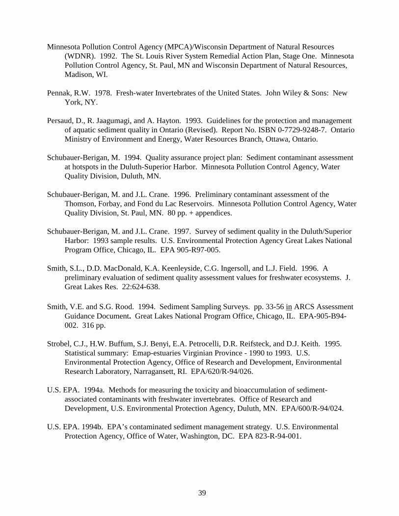
39

Minnesota Pollution Control Agency (MPCA)/Wisconsin Department of Natural Resources(WDNR). 1992. The St. Louis River System Remedial Action Plan, Stage One. MinnesotaPollution Control Agency, St. Paul, MN and Wisconsin Department of Natural Resources,Madison, WI.

Pennak, R.W. 1978. Fresh-water Invertebrates of the United States. John Wiley & Sons: NewYork, NY.

Persaud, D., R. Jaagumagi, and A. Hayton. 1993. Guidelines for the protection and managementof aquatic sediment quality in Ontario (Revised). Report No. ISBN 0-7729-9248-7. OntarioMinistry of Environment and Energy, Water Resources Branch, Ottawa, Ontario.

Schubauer-Berigan, M. 1994. Quality assurance project plan: Sediment contaminant assessmentat hotspots in the Duluth-Superior Harbor. Minnesota Pollution Control Agency, WaterQuality Division, Duluth, MN.

Schubauer-Berigan, M. and J.L. Crane. 1996. Preliminary contaminant assessment of theThomson, Forbay, and Fond du Lac Reservoirs. Minnesota Pollution Control Agency, WaterQuality Division, St. Paul, MN. 80 pp. + appendices.

Schubauer-Berigan, M. and J.L. Crane. 1997. Survey of sediment quality in the Duluth/SuperiorHarbor: 1993 sample results. U.S. Environmental Protection Agency Great Lakes NationalProgram Office, Chicago, IL. EPA 905-R97-005.

Smith, S.L., D.D. MacDonald, K.A. Keenleyside, C.G. Ingersoll, and L.J. Field. 1996. Apreliminary evaluation of sediment quality assessment values for freshwater ecosystems. J.Great Lakes Res. 22:624-638.

Smith, V.E. and S.G. Rood. 1994. Sediment Sampling Surveys. pp. 33-56 in ARCS AssessmentGuidance Document. Great Lakes National Program Office, Chicago, IL. EPA-905-B94-002. 316 pp.

Strobel, C.J., H.W. Buffum, S.J. Benyi, E.A. Petrocelli, D.R. Reifsteck, and D.J. Keith. 1995.Statistical summary: Emap-estuaries Virginian Province - 1990 to 1993. U.S.Environmental Protection Agency, Office of Research and Development, EnvironmentalResearch Laboratory, Narragansett, RI. EPA/620/R-94/026.

U.S. EPA. 1994a. Methods for measuring the toxicity and bioaccumulation of sediment-associated contaminants with freshwater invertebrates. Office of Research andDevelopment, U.S. Environmental Protection Agency, Duluth, MN. EPA/600/R-94/024.

U.S. EPA. 1994b. EPA’s contaminated sediment management strategy. U.S. EnvironmentalProtection Agency, Office of Water, Washington, DC. EPA 823-R-94-001.

40

FIGURES

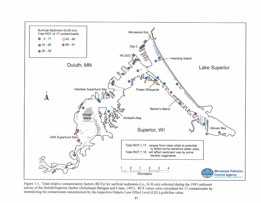
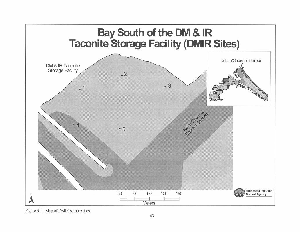
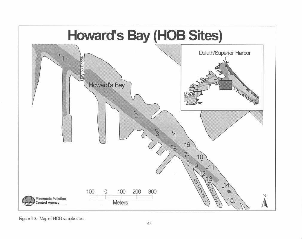
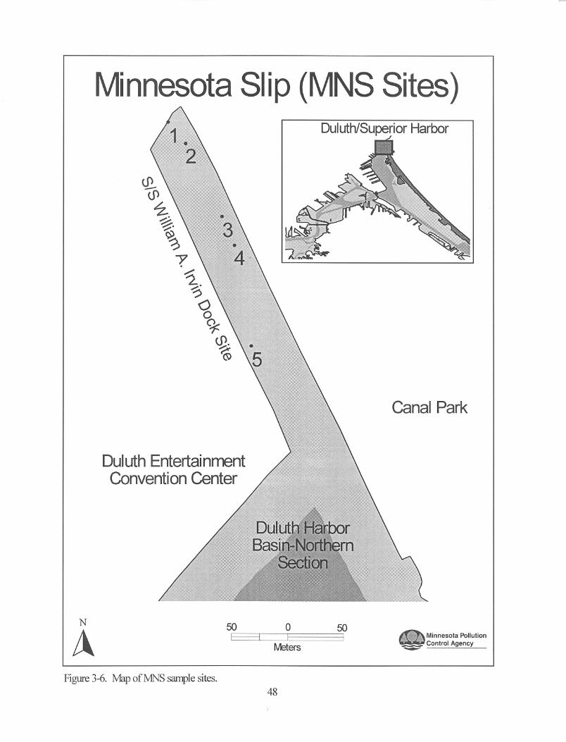
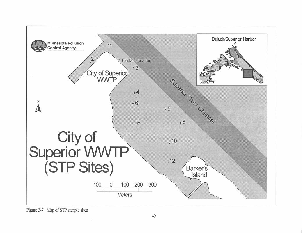
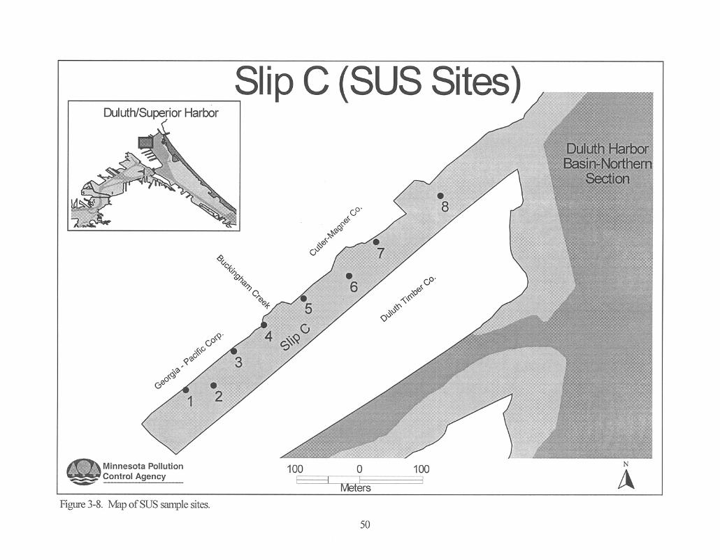
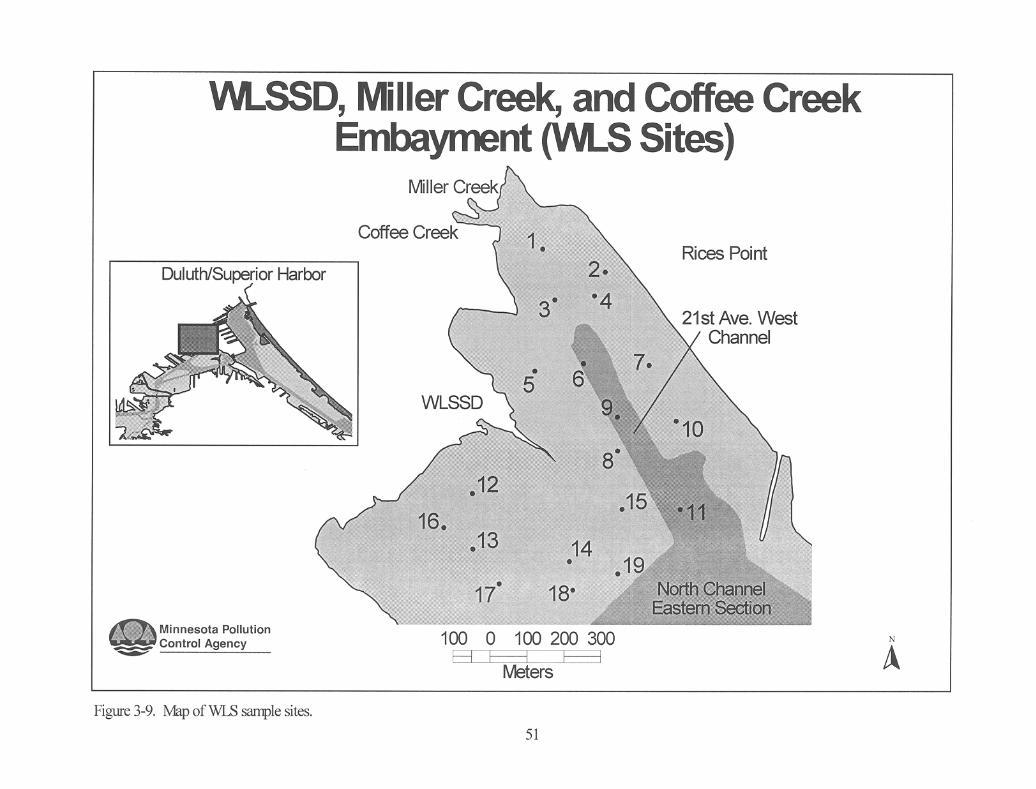
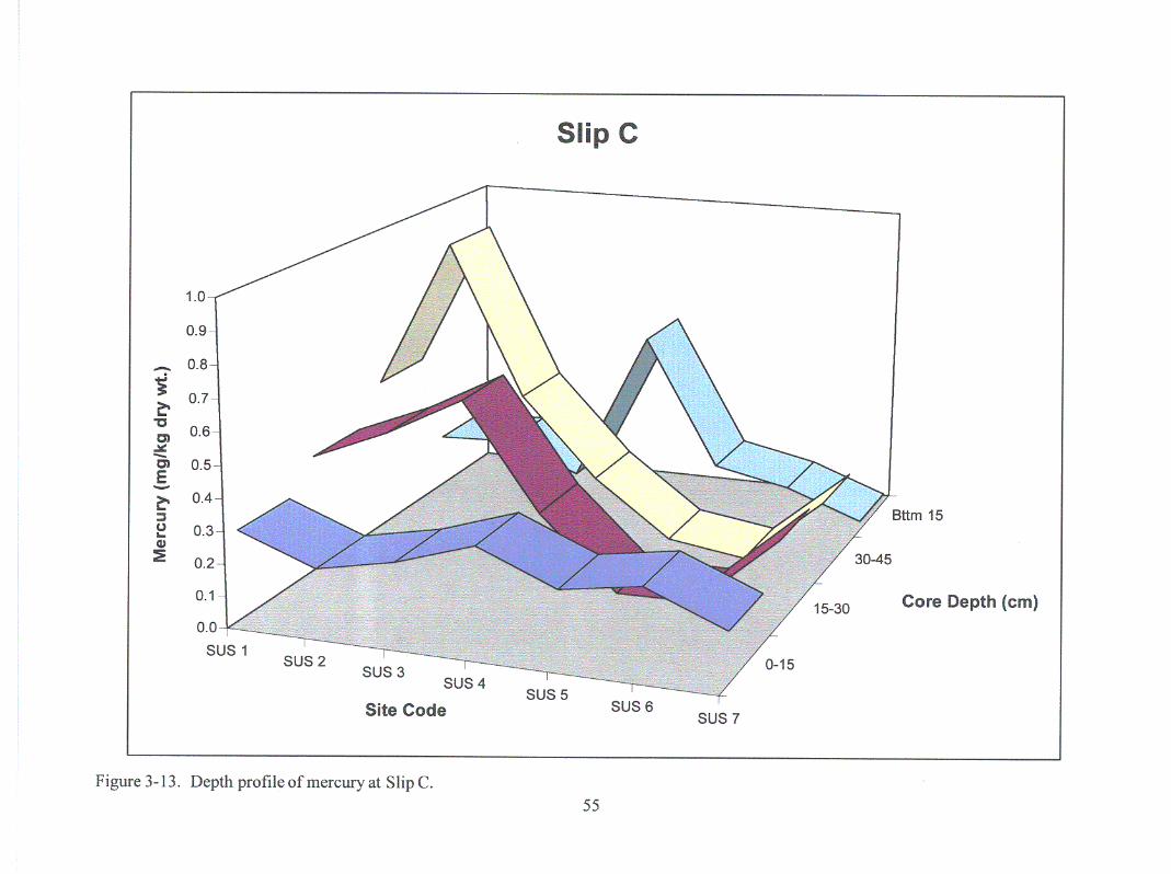
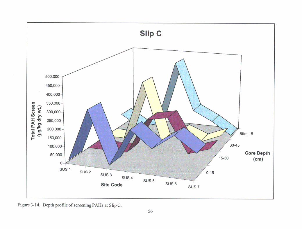
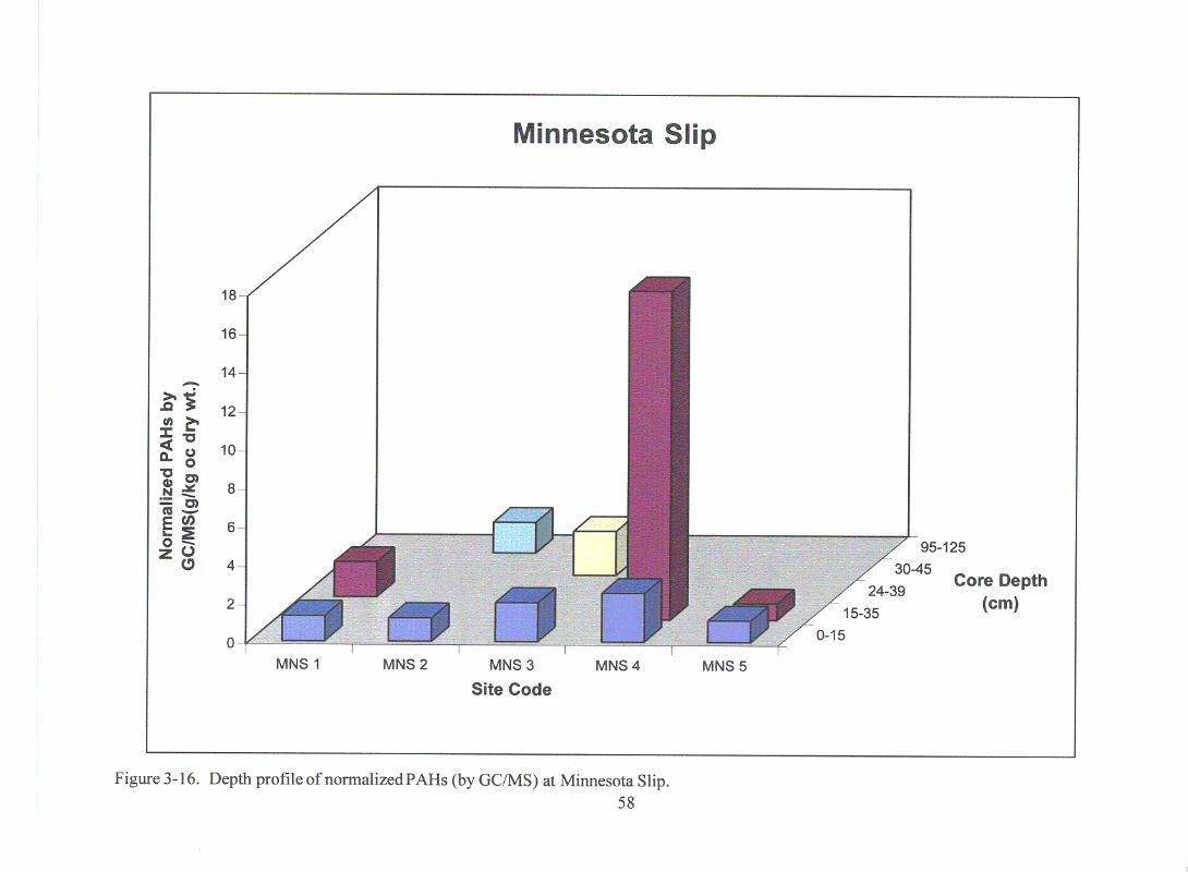
61

TABLES

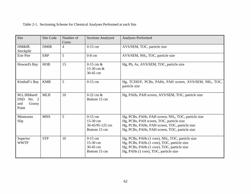
62

Table 2-1. Sectioning Scheme for Chemical Analyses Performed at each Site

Site Site Code Number ofCores

Sections Analyzed Analyses Performed

DM&IRStockpile

DMIR 4 0-15 cm AVS/SEM, TOC, particle size

Erie Pier ERP 5 0-8 cm AVS/SEM, NH3, TOC, particle size

Howard's Bay HOB 15 0-15 cm &15-30 cm &30-45 cm

Hg, Pb, As, AVS/SEM, TOC, particle size

Kimball’s Bay KMB 5 0-15 cm Hg, TCDD/F, PCBs, PAHs, PAH screen, AVS/SEM, NH3, TOC,particle size

M.L.Hibbard/DSD No. 2and GrassyPoint

MLH 10 0-22 cm &Bottom 15 cm

Hg, PAHs, PAH screen, AVS/SEM, TOC, particle size

MinnesotaSlip

MNS 5 0-15 cm15-30 cm30-45/95-125 cmBottom 15 cm

Hg, PCBs, PAHs, PAH screen, NH3, TOC, particle sizeHg, PCBs, PAH screen, TOC, particle sizeHg, PCBs, PAHs, PAH screen, TOC, particle sizeHg, PCBs, PAHs, PAH screen, TOC, particle size

SuperiorWWTP

STP 10 0-15 cm15-30 cm30-45 cmBottom 15 cm

Hg, PCBs, PAHs (1 core), NH3, TOC, particle sizeHg, PCBs, PAHs (1 core), TOC, particle sizeHg, PCBs, PAHs (1 core), TOC, particle sizeHg, PAHs (1 core), TOC, particle size

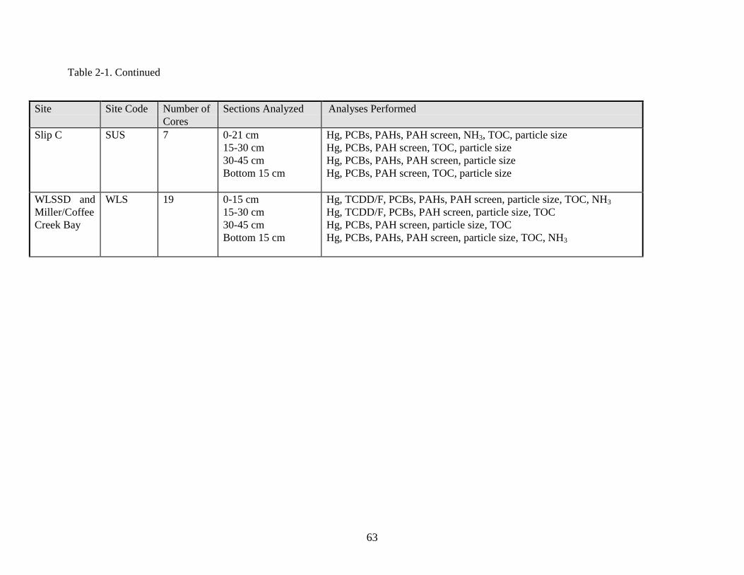
63

Table 2-1. Continued

Site Site Code Number ofCores

Sections Analyzed Analyses Performed

Slip C SUS 7 0-21 cm15-30 cm30-45 cmBottom 15 cm

Hg, PCBs, PAHs, PAH screen, NH3, TOC, particle sizeHg, PCBs, PAH screen, TOC, particle sizeHg, PCBs, PAHs, PAH screen, particle sizeHg, PCBs, PAH screen, TOC, particle size

WLSSD andMiller/CoffeeCreek Bay

WLS 19 0-15 cm15-30 cm30-45 cmBottom 15 cm

Hg, TCDD/F, PCBs, PAHs, PAH screen, particle size, TOC, NH3Hg, TCDD/F, PCBs, PAH screen, particle size, TOCHg, PCBs, PAH screen, particle size, TOCHg, PCBs, PAHs, PAH screen, particle size, TOC, NH3

64

Table 2-2. Summary of Sediment Analytical Methods

Analyte Method(description)

Sample cleanup

2,3,7,8-TCDD &2,3,7,8-TCDF

SW846(GC/MS)

acid/base, AgNO3/silica gel,Cu, alumina, carbon

PCBs EPA SW846--8081(capillary column GC)

Florisil

PAHs Method 8270(capillary column GC)

GPC

Hg EPA 245.5(cold vapor AAS)

N/A

As EPA 206.5(hydride generation)

N/A

Pb Nitric acid/hydrogenperoxide digestion.Flame/furnace AAS

N/A

AVS Allen et al. (1991)(photometer)

N/A

SEM Allen et al. (1991)(atomic absorption)

N/A

Ammonia KC1 extraction (Soilsmethod 33.3:exchangeable ammonia)

N/A

TOC Total organic carbon*Sample ignition method 1

N/A

PAH fluorometricanalysis

N/A None

*Technical Report EPA/COE - 81-1.

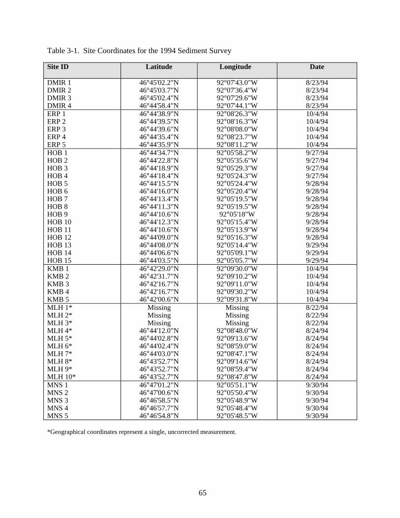
65

Table 3-1. Site Coordinates for the 1994 Sediment Survey

Site ID Latitude Longitude Date

DMIR 1 46°45'02.2"N 92°07'43.0"W 8/23/94DMIR 2 46°45'03.7"N 92°07'36.4"W 8/23/94DMIR 3 46°45'02.4"N 92°07'29.6"W 8/23/94DMIR 4 46°44'58.4"N 92°07'44.1"W 8/23/94ERP 1 46°44'38.9"N 92°08'26.3"W 10/4/94ERP 2 46°44'39.5"N 92°08'16.3"W 10/4/94ERP 3 46°44'39.6"N 92°08'08.0"W 10/4/94ERP 4 46°44'35.4"N 92°08'23.7"W 10/4/94ERP 5 46°44'35.9"N 92°08'11.2"W 10/4/94HOB 1 46°44'34.7"N 92°05'58.2"W 9/27/94HOB 2 46°44'22.8"N 92°05'35.6"W 9/27/94HOB 3 46°44'18.9"N 92°05'29.3"W 9/27/94HOB 4 46°44'18.4"N 92°05'24.3"W 9/27/94HOB 5 46°44'15.5"N 92°05'24.4"W 9/28/94HOB 6 46°44'16.0"N 92°05'20.4"W 9/28/94HOB 7 46°44'13.4"N 92°05'19.5"W 9/28/94HOB 8 46°44'11.3"N 92°05'19.5"W 9/28/94HOB 9 46°44'10.6"N 92°05'18"W 9/28/94HOB 10 46°44'12.3"N 92°05'15.4"W 9/28/94HOB 11 46°44'10.6"N 92°05'13.9"W 9/28/94HOB 12 46°44'09.0"N 92°05'16.3"W 9/28/94HOB 13 46°44'08.0"N 92°05'14.4"W 9/29/94HOB 14 46°44'06.6"N 92°05'09.1"W 9/29/94HOB 15 46°44'03.5"N 92°05'05.7"W 9/29/94KMB 1 46°42'29.0"N 92°09'30.0"W 10/4/94KMB 2 46°42'31.7"N 92°09'10.2"W 10/4/94KMB 3 46°42'16.7"N 92°09'11.0"W 10/4/94KMB 4 46°42'16.7"N 92°09'30.2"W 10/4/94KMB 5 46°42'00.6"N 92°09'31.8"W 10/4/94MLH 1* Missing Missing 8/22/94MLH 2* Missing Missing 8/22/94MLH 3* Missing Missing 8/22/94MLH 4* 46°44'12.0"N 92°08'48.0"W 8/24/94MLH 5* 46°44'02.8"N 92°09'13.6"W 8/24/94MLH 6* 46°44'02.4"N 92°08'59.0"W 8/24/94MLH 7* 46°44'03.0"N 92°08'47.1"W 8/24/94MLH 8* 46°43'52.7"N 92°09'14.6"W 8/24/94MLH 9* 46°43'52.7"N 92°08'59.4"W 8/24/94MLH 10* 46°43'52.7"N 92°08'47.8"W 8/24/94MNS 1 46°47'01.2"N 92°05'51.1"W 9/30/94MNS 2 46°47'00.6"N 92°05'50.4"W 9/30/94MNS 3 46°46'58.5"N 92°05'48.9"W 9/30/94MNS 4 46°46'57.7"N 92°05'48.4"W 9/30/94MNS 5 46°46'54.8"N 92°05'48.5"W 9/30/94

*Geographical coordinates represent a single, uncorrected measurement.

66

Table 3-1. Continued

Site ID Latitude Longitude Date

STP 1 46°43'50.9"N 92°04'14.4"W 9/29/94STP 2 46°43'46.7"N 92°04'21.3"W 9/29/94STP 3 46°43'45.4"N 92°04'06.7"W 9/29/94STP 4 46°43'39.5"N 92°04'06.3"W 9/29/94STP 5 46°43'35.5"N 92°03'55.9"W 9/30/94STP 6 46°43'37.0"N 92°04'06.9"W 10/3/94STP 7 46°43'32.5"N 92°04'04.9"W 10/3/94STP 8 46°43'32.3"N 92°03'50.8"W 10/3/94STP 10 46°43'27.5"N 92°03'54.5"W 10/3/94STP 12 46°43'23.1"N 92°03'55.2"W 10/3/94SUS 1 46°46'16.4"N 92°06'39.2"W 9/22/94SUS 2 46°46'16.6"N 92°06'37.2"W 9/22/94SUS 3 46°46'18.3"N 92°06'35.7"W 9/22/94SUS 4 46°46'19.6"N 92°06'33.5"W 9/22/94SUS 5 46°46'20.9"N 92°06'30.6"W 9/22/94SUS 6 46°46'22"N 92°06'27.3"W 9/22/94SUS 7 46°46'23.7"N 92°06'25.3"W 10/3/94SUS 8 46°46'26"N 92°06'20.6"W 10/3/94WLS 1 46°45'46.6"N 92°07'11.5"W 9/21/94WLS 2 46°45'44.5"N 92°07'03.5"W 9/21/94WLS 3 46°45'42.1"N 92°07'10.0"W 9/21/94WLS 4 46°45'42.4"N 92°07'04.9"W 9/23/94WLS 5 46°45'35.9"N 92°07'12.6"W 9/23/94WLS 6 46°45'36.5"N 92°07'06.4"W 9/23/94WLS 7 46°45'36.3"N 92°06'58.0"W 9/23/94WLS 8 46°45'28.8"N 92°07'02.1"W 9/23/94WLS 9 46°45'31.8"N 92°07'02.1"W 9/23/94WLS 10 46°45'31.4"N 92°06'54.6"W 9/23/94WLS 11 46°45'23.6"N 92°06'54.2"W 9/23/94WLS 12 46°45'25.2"N 92°07'20.7"W 9/26/94WLS 13 46°45'20.3"N 92°07'20.7"W 9/26/94WLS 14 46°45'19.1"N 92°07'08.4"W 9/26/94WLS 15 46°45'23.7"N 92°07'01.6"W 9/26/94WLS 16* 46°45'22.2"N 92°07'24.4"W 9/26/94WLS 17* 46°45'17.2"N 92°07'17.4"W 9/26/94WLS 18* 46°45'16.6"N 92°07'08.0"W 9/27/94WLS 19* 46°45'18.0"N 92°06'01.0"W 9/27/94

* Geographical coordinates result from a single, uncorrected measurement at starred sites

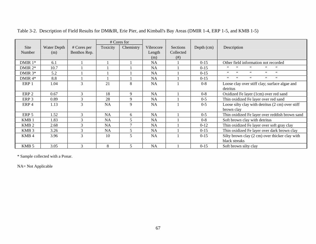
67

Table 3-2. Description of Field Results for DM&IR, Erie Pier, and Kimball's Bay Areas (DMIR 1-4, ERP 1-5, and KMB 1-5)

# Cores forSite

NumberWater Depth

(m)# Cores per

Benthos Rep.Toxicity Chemistry Vibrocore

Length(m)

SectionsCollected

(#)

Depth (cm) Description

DMIR 1* 6.1 1 1 1 NA 1 0-15 Other field information not recordedDMIR 2* 10.7 1 1 1 NA 1 0-15 “ “ “ “ “DMIR 3* 5.2 1 1 1 NA 1 0-15 “ “ “ “ “DMIR 4* 8.8 1 1 1 NA 1 0-15 “ “ “ “ “

ERP 1 1.04 3 21 8 NA 1 0-8 Loose clay over stiff clay; surface algae anddetritus

ERP 2 0.67 3 18 9 NA 1 0-8 Oxidized Fe layer (1cm) over red sandERP 3 0.89 3 28 9 NA 1 0-5 Thin oxidized Fe layer over red sandERP 4 1.13 3 NA 9 NA 1 0-5 Loose silty clay with detritus (2 cm) over stiff

brown clayERP 5 1.52 3 NA 6 NA 1 0-5 Thin oxidized Fe layer over reddish brown sandKMB 1 1.83 3 NA 5 NA 1 0-8 Soft brown clay with detritusKMB 2 2.68 3 NA 7 NA 1 0-12 Thin oxidized Fe layer over soft gray clayKMB 3 3.26 3 NA 5 NA 1 0-15 Thin oxidized Fe layer over dark brown clayKMB 4 3.96 3 10 5 NA 1 0-15 Silty brown clay (2 cm) over thicker clay with

black streaksKMB 5 3.05 3 8 5 NA 1 0-15 Soft brown silty clay

* Sample collected with a Ponar.

NA= Not Applicable

68

Table 3-3. Description of Field Results for Howard's Bay (HOB 1-15)

# Cores forSite

NumberWater Depth

(m)# Cores per

Benthos Rep.Toxicity Chemistry Vibrocore

Length(m)

SectionsCollected

(#)

Depth (cm) Description

HOB 1 9.75 3 NA 4 0.20 123

0-50-5 (VC)

5-20 (VC)

Brown sandy clay (slight oil sheen)Brown sandy clay (slight oil sheen)Brown sandy clay (slight oil sheen)

HOB 2 8.23 3 NA 3 1.38 1

23

0-15

15-3030-45

Sandy orange clay, some detritus (slight oilsheen)Loose sandy clay (slight oil sheen)Loose sandy clay with wood and detritus(slight oil sheen)

HOB 3 8.75 2 NA 3 0.45 1

2

3

0-15

15-30

30-45

Sand with shiny particles (5 cm) over pinkand brown claySoft brown clay with plant fibers (slight oilsheen)Stiff, brick-colored clay

HOB 4 4.33 2 NA 3 1.00 123

0-1515-3030-45

Sand/grit (3 cm) over pink and brown claySoft pink and brown claySoft pink and brown clay with wood detritus

HOB 5 8.90 2 NA 4 0.45 1

23

0-15

15-3030-45

Loose, flocculant, oxidized Fe (3 cm) oversoft brown clayDark brown clay (10 cm) over red clayRed clay (5 cm) over dark brown clay withsome oil smears

HOB 6 1.28 3 NA 3 0.45 1

23

0-15

15-3030-45

Dark gritty sand (2 mm) over red clay (5 cm)over black clay with oily coal chunks (5 cm)over red sandClay with sand and coal chunks, no oilCoarse red sand, few pebbles

HOB 7 8.20 2 10 3 0.82 1

23

0-15

15-3030-45

Fluffy silt/clay with black grit (5 cm) overbrown claySandy brown clay, some oil and detritusUniform sandy brown clay with somedetritus, less oil

NA= Not ApplicableVC= Vibrocorer

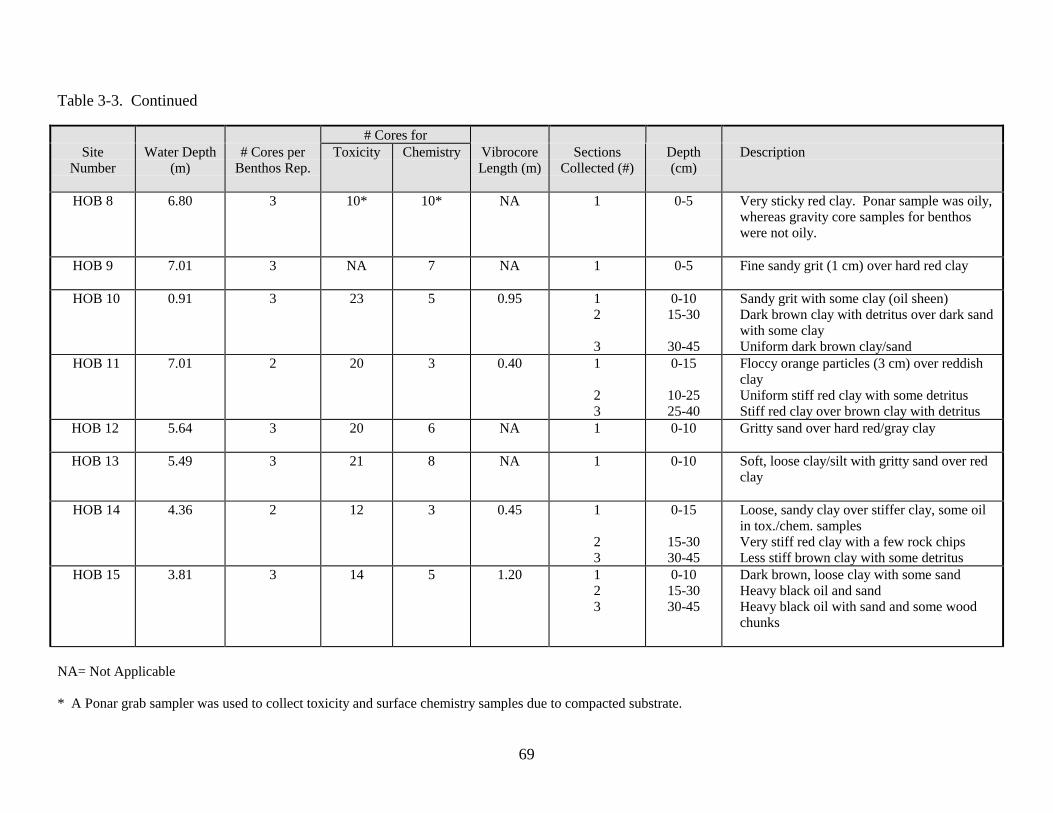
69

Table 3-3. Continued

# Cores forSite

NumberWater Depth

(m)# Cores per

Benthos Rep.Toxicity Chemistry Vibrocore

Length (m)Sections

Collected (#)Depth(cm)

Description

HOB 8 6.80 3 10* 10* NA 1 0-5 Very sticky red clay. Ponar sample was oily,whereas gravity core samples for benthoswere not oily.

HOB 9 7.01 3 NA 7 NA 1 0-5 Fine sandy grit (1 cm) over hard red clay

HOB 10 0.91 3 23 5 0.95 12

3

0-1015-30

30-45

Sandy grit with some clay (oil sheen)Dark brown clay with detritus over dark sandwith some clayUniform dark brown clay/sand

HOB 11 7.01 2 20 3 0.40 1

23

0-15

10-2525-40

Floccy orange particles (3 cm) over reddishclayUniform stiff red clay with some detritusStiff red clay over brown clay with detritus

HOB 12 5.64 3 20 6 NA 1 0-10 Gritty sand over hard red/gray clay

HOB 13 5.49 3 21 8 NA 1 0-10 Soft, loose clay/silt with gritty sand over redclay

HOB 14 4.36 2 12 3 0.45 1

23

0-15

15-3030-45

Loose, sandy clay over stiffer clay, some oilin tox./chem. samplesVery stiff red clay with a few rock chipsLess stiff brown clay with some detritus

HOB 15 3.81 3 14 5 1.20 123

0-1015-3030-45

Dark brown, loose clay with some sandHeavy black oil and sandHeavy black oil with sand and some woodchunks

NA= Not Applicable

* A Ponar grab sampler was used to collect toxicity and surface chemistry samples due to compacted substrate.

70

Table 3-4. Description of Field Results for M.L. Hibbard/DSD No. 2 Plant and Grassy Point Embayment (MLH 1-10)

# Cores forSite

NumberWater Depth

(m)# Cores per

Benthos Rep.Toxicity Chemistry Vibrocore

Length(m)

SectionsCollected

(#)

Depth (cm) Description

MLH 1 1.52 1 10 2 0.4 1Bottom

0-13.525-40

Gritty, uniform black/brown sedimentSame as upper section

MLH 2 1.04 1 6 2 0.95 1

Bottom

0-22

80-95

Silt with ash throughout, strong sulfide odor,slight oil sheenUniform, dark granular fly ash

MLH 3 1.52 1 5 2 0.52 1Bottom

0-2037-52

Ash with some silt, strong sulfide odorFine clay/ash over wood chips and detritus

MLH 4 2.13 1 7 2 0.50 1Bottom

0-20.530-50

Very fine brown clay/silt, some ash, oil sheenSoft brown clay over coarse brown sand withwood chips and detritus

MLH 5 2.26 1 6 2 0.47 1

Bottom

0-17.5

32-47

Soft brown clay/silt with oxidized Fe layer onsurfaceThick brown clay over black ash/wood chips(5 cm)

MLH 6 1.92 1 6 2 0.40 1

Bottom

0-21

25-40

Reddish brown sand with black wood chips,grit, and detritusUniform sand with fly ash

MLH 7 2.32 1 NA 2 0.87 1

Bottom

0-17

72-87

Soft, light brown sandy clay with some fineblack granular materialBrown sand with some clay

MLH 8 2.44 1 NA 2 0.76 1Bottom

0-15.560-76

Soft brown clay/silt with some wood fibersCoarse brown sand

MLH 9 2.53 1 NA 2 0.79 1

Bottom

0-22

52-79

Soft brown silty clay with some wood chipsand black striationsGray clay and wood fibers (12 cm) overdensely packed wood fibers

MLH 10 3.20 1 NA 2 0.95 1Bottom

0-2175-95

Soft brown silty clayBrown clay with black bands ofundecomposed organic fibers

NA= Not Applicable

71

Table 3-5. Description of Field Results for Minnesota Slip (MNS 1-5)

# Cores forSite

NumberWater

Depth (m)# Cores per

Benthos Rep.Toxicity Chemistry Vibrocore

Length (m)Sections

Collected (#)Depth (cm) Description

MNS 1 5.03 3 17 6 0.54 1234

0-109-24

24-3939-54

Soft, oily silt/clayBlack, oily sand/silt/clay with some detritusBlack, very oily sand/clayVery oily, stiffer black sand/clay

MNS 2 5.00 3 NA 6 1.60 1234

0-1215-30

95-125145-160

Loose, dark brown silt/clayBlack, oily, sandy clay with some detritusBlack, oily, sandy clayUniform, black oily sand (with white bits andred fibers)

MNS 3 5.06 3 13 3 0.60 123

4

0-1515-3030-45

45-60

Gritty silty/clay over silt and some oil/detritusSoft, oily silt/clay with some detritusSoft, brown clay (3 cm) over oily detritus (5cm) over non-oily reddish sandOily reddish sand, little detritus

MNS 4 4.88 3 NA 4 0.60 1234

0-150-15 (VC)

15-3030-45

Loose, oily clay (5 cm) over stiff clayLoose clay (3 cm) over oily sand with detritusVery coarse sand, slightly oily, large rocksFine sand, no oil, some detritus

MNS 5 4.27 3 NA 5 0.65 1

234

0-10

5-2020-3535-50

Silt with detritus over soft clay (slight oilsheen)Coarse red sand over detritus over sand, no oilVery coarse, rocky sandRocks and detritus with oil smell (slight oilsheen) over coarse sand

NA= Not ApplicableVC= Vibrocorer

72

Table 3-6. Description of Field Results for City of Superior WWTP Embayment (STP 1-8, STP 10, STP 12)

# Cores forSite

NumberWater Depth

(m)# Cores per

Benthos Rep.Toxicity Chemistry Vibrocore

Length (m)SectionsCollected

(#)

Depth (cm) Description

STP 1 7.01 2 22 4 0.82 1

23

0-15

15-3030-45

Floccy orange mat (3 cm) atop loose sandyclay; tox./chem samples had slight oil sheenLoose dark brown clay with detritusDark brown clay/sand, slight oil sheen

STP 2 4.02 2 NA 7 0.25 1

2

0-15

10-25

Dark brown clay/sand (10 cm) over moregray/black clay/sandSand with a bit of clay, strong sulfide odorand oil

STP 3 3.60 2 (A)3 (B&C)

15 6 0.60 1

23

0-10

15-3030-45

Sandy grit atop clay/sand with some detritus,slight oil sheenFine brown sand with some detritusFine brown sand (5 cm) over coarse red sand

STP 4 2.44 2 13 6 0.96 1

23

0-15

15-3030-45

Oxidized granular layer (5 cm) over soft,gray-brown clayey sandSoft, uniform brown clay, little detritusStiffer, uniform brown clay

STP 5 3.17 2 NA 4 NA 1 0-15 Oxidized Fe layer (1 cm) over soft brownclay/silt

STP 6 2.13 2 13 3 0.38 1

23

0-15

7-2323-38

Oxidized Fe layer atop soft silt/clay withdetritusLarge wood chunks over soft silt/clayStiffer brown clay

STP 7 2.31 2 12 4 0.23 1

2

0-15

5-23

Thin oxidized Fe layer over red clay (7 cm)over brown clay, slight oil sheenLoose brown clay with wood chunks and oilsheen over sand

STP 8 3.20 2 NA 4 0.30 1

23

0-15

0-15(VC)15-30

Thin oxidized Fe layer over silt/clay overbrown clayLoose brown clay with oil sheenBrown soft clay with oil sheen, red sand atbottom 2 cm

NA= Not Applicable

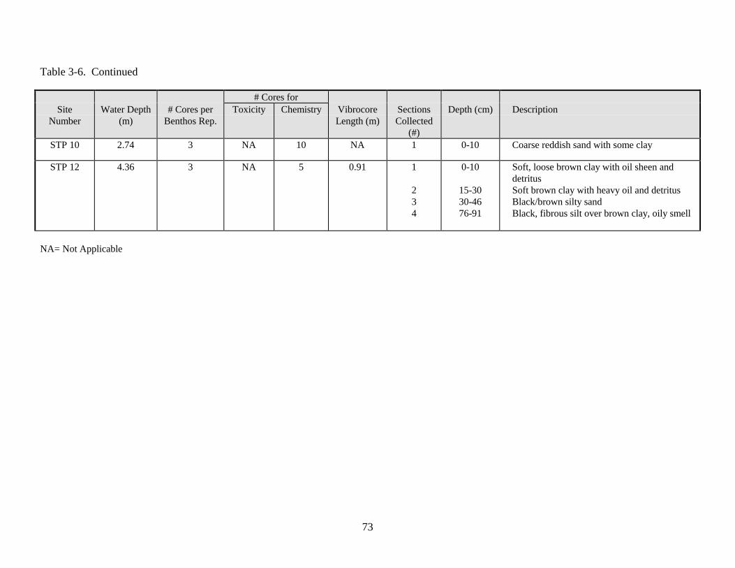
73

Table 3-6. Continued

# Cores forSite

NumberWater Depth

(m)# Cores per

Benthos Rep.Toxicity Chemistry Vibrocore

Length (m)SectionsCollected

(#)

Depth (cm) Description

STP 10 2.74 3 NA 10 NA 1 0-10 Coarse reddish sand with some clay

STP 12 4.36 3 NA 5 0.91 1

234

0-10

15-3030-4676-91

Soft, loose brown clay with oil sheen anddetritusSoft brown clay with heavy oil and detritusBlack/brown silty sandBlack, fibrous silt over brown clay, oily smell

NA= Not Applicable

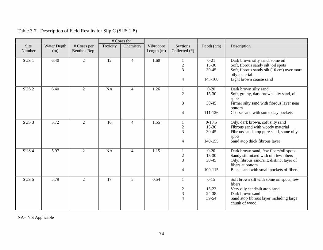
74

Table 3-7. Description of Field Results for Slip C (SUS 1-8)

# Cores forSite

NumberWater Depth

(m)# Cores per

Benthos Rep.Toxicity Chemistry Vibrocore

Length (m)Sections

Collected (#)Depth (cm) Description

SUS 1 6.40 2 12 4 1.60 123

4

0-2115-3030-45

145-160

Dark brown silty sand, some oilSoft, fibrous sandy silt, oil spotsSoft, fibrous sandy silt (10 cm) over moreoily materialLight brown coarse sand

SUS 2 6.40 2 NA 4 1.26 12

3

4

0-2015-30

30-45

111-126

Dark brown silty sandSoft, grainy, dark brown silty sand, oilspotsFirmer silty sand with fibrous layer nearbottomCoarse sand with some clay pockets

SUS 3 5.72 2 10 4 1.55 123

4

0-18.515-3030-45

140-155

Oily, dark brown, soft silty sandFibrous sand with woody materialFibrous sand atop pure sand, some oilyspotsSand atop thick fibrous layer

SUS 4 5.97 2 NA 4 1.15 123

4

0-2015-3030-45

100-115

Dark brown sand, few fibers/oil spotsSandy silt mixed with oil, few fibersOily, fibrous sand/silt; distinct layer offibers at bottomBlack sand with small pockets of fibers

SUS 5 5.79 2 17 5 0.54 1

234

0-15

15-2324-3839-54

Soft brown silt with some oil spots, fewfibersVery oily sand/silt atop sandDark brown sandSand atop fibrous layer including largechunk of wood

NA= Not Applicable

75

Table 3-7. Continued

# Cores forSite

NumberWater Depth

(m)# Cores per

Benthos Rep.Toxicity Chemistry Vibrocore

Length (m)SectionsCollected

(#)

Depth (cm) Description

SUS 6 6.76 2 NA 4 1.30 12

34

0-18.515-30

30-45115-130

Oily, black-gray sandRust-brown sand with white specks, somesticksSand with a few fibersSand with a few fibers

SUS 7 7.62 3 17 9 0.78 12

34

0-515-30

30-4563-78

Wood and plant detritus atop red sandOily soft brown clay with detritus over redsandReddish sand and wood detritus, oil smellRed sand, no oil

SUS 8 7.32 1 NA NA NA None 0-10 Coarse sand; could only collect 1 replicate forbenthos

NA= Not Applicable

76

Table 3-8. Description of Field Results for WLSSD and Miller/Coffee Creek Embayment (WLS 1-20)

# Cores forSite

NumberWater Depth

(m)# Cores per

BenthosRep.

Toxicity Chemistry VibrocoreLength (m)

SectionsCollected

(#)

Depth (cm) Description

WLS 1 2.29 1 10 4 2.04 123

4

0-1515-3030-45

189-204

Soft brown silt, slight oil odorSoft, fibrous silt with heavy oilBlack oil and fibers (5 cm) over softbrown siltUniform brownish-gray clay

WLS 2 2.49 2 11 5 1.82 1

234

0-15

15-3030-45

167-182

Soft brown silt, some oil and fibrousmaterialUniform gray-brown clay, slightly oilyStiff, gray-brown clayUniform dark brown clay

WLS 3 2.08 2 9 3 1.88 1

234

0-18.5

15-3030-45

173-188

Gray-brown silt/clay mixture withfibersSandy with very fine silt, few fibersSilty clay with some wood chunksDark brown clay with plant detritus

WLS 4 2.34 2 8 4 1.21 1

2

34

0-20

15-30

30-45105-120

Loose, brown silty clay, slight oil, littledetritusSand with little detritus, no oil, somestonesSimilar to 15-30 cm sectionGrayish-brown clay with a few stones

WLS 5 1.92 2 NA 3 1.50 12

3

4

0-1815-30

30-45

135-150

Soft brown silty clay, some oilBrown silty clay, some oil; coal chunksand fibers at bottom of sectionCoal/sand/clay with abundant oilbloomsVery fibrous, organic brown stratumwith some larger wood chips

NA= Not Applicable

77

Table 3-8. Continued

# Cores forSite

NumberWater Depth

(m)# Cores per

Benthos Rep.Toxicity Chemistry Vibrocore

Length (m)SectionsCollected

(#)

Depth (cm) Description

WLS 6 6.80 2 6 4 2.50 1234

0-1915-3030-45

235-250

Loose silty clay with black oil streaksSoft brown silt with oil sheenSame as 15-30 cm sectionSoft, gray clay with fibers

WLS 7 5.33 2 NA 4 0.5 1234

0-205-20

20-3535-50

Soft brown silt/clay with oil spotsSoft silt with a lot of oilLoose silt/clay (5 cm) over oily sandSand with oily coal chunks and small redclay pieces

WLS 8 3.28 2 5 4 1.05 1234

0-2015-3030-45

90-105

Very oily silty clay with fibersGrayish-brown, stiff fibrous clayStiff gray-brown clay with fewer fibersPeaty organic cattail-like detritus

WLS 9 7.92 2 NA 3 1.60 12

34

0-2015-30

30-45145-160

Soft brown silt/clay with oil at bottom 5 cmHeavy oil (5 cm) over fibrous clay with oilstreaksUniform, soft gray fibrous clayUniform, stiff fibrous clay

WLS 10 1.98 2 NA 5 1.50 1234

0-1515-3030-45

135-150

Brown soft silt over very oily layer (3 cm)Uniform clay/sand, no visible oilUniform sandy clay, no visible oilDry brownish sand, no fibers present

NA= Not Applicable

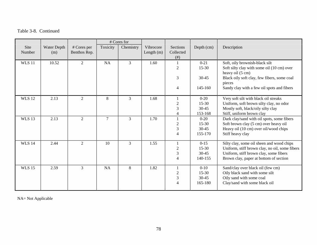
78

Table 3-8. Continued

# Cores forSite

NumberWater Depth

(m)# Cores per

Benthos Rep.Toxicity Chemistry Vibrocore

Length (m)SectionsCollected

(#)

Depth (cm) Description

WLS 11 10.52 2 NA 3 1.60 12

3

4

0-2115-30

30-45

145-160

Soft, oily brownish-black siltSoft silty clay with some oil (10 cm) overheavy oil (5 cm)Black oily soft clay, few fibers, some coalpiecesSandy clay with a few oil spots and fibers

WLS 12 2.13 2 8 3 1.68 1234

0-2015-3030-45

153-168

Very soft silt with black oil streaksUniform, soft brown silty clay, no odorMostly soft, black/oily silty clayStiff, uniform brown clay

WLS 13 2.13 2 7 3 1.70 1234

0-2015-3030-45

155-170

Dark clay/sand with oil spots, some fibersSoft brown clay (5 cm) over heavy oilHeavy oil (10 cm) over oil/wood chipsStiff heavy clay

WLS 14 2.44 2 10 3 1.55 1234

0-1515-3030-45

140-155

Silty clay, some oil sheen and wood chipsUniform, stiff brown clay, no oil, some fibersUniform, stiff brown clay, some fibersBrown clay, paper at bottom of section

WLS 15 2.59 3 NA 8 1.82 1234

0-1015-3030-45

165-180

Sand/clay over black oil (few cm)Oily black sand with some siltOily sand with some coalClay/sand with some black oil

NA= Not Applicable

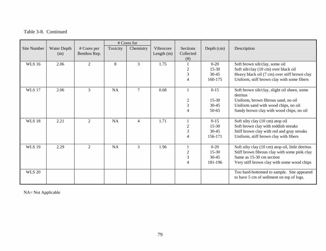
79

Table 3-8. Continued

# Cores forSite Number Water Depth

(m)# Cores per

Benthos Rep.Toxicity Chemistry Vibrocore

Length (m)SectionsCollected

(#)

Depth (cm) Description

WLS 16 2.06 2 8 3 1.75 1234

0-2015-3030-45

160-175

Soft brown silt/clay, some oilSoft silt/clay (10 cm) over black oilHeavy black oil (7 cm) over stiff brown clayUniform, stiff brown clay with some fibers

WLS 17 2.06 3 NA 7 0.68 1

234

0-15

15-3030-4550-65

Soft brown silt/clay, slight oil sheen, somedetritusUniform, brown fibrous sand, no oilUniform sand with wood chips, no oilSandy brown clay with wood chips, no oil

WLS 18 2.21 2 NA 4 1.71 1234

0-1515-3030-45

156-171

Soft silty clay (10 cm) atop oilSoft brown clay with reddish streaksStiff brown clay with red and gray streaksUniform, stiff brown clay with fibers

WLS 19 2.29 2 NA 3 1.96 1234

0-2015-3030-45

181-196

Soft silty clay (10 cm) atop oil, little detritusStiff brown fibrous clay with some pink claySame as 15-30 cm sectionVery stiff brown clay with some wood chips

WLS 20 Too hard-bottomed to sample. Site appearedto have 5 cm of sediment on top of logs.

NA= Not Applicable

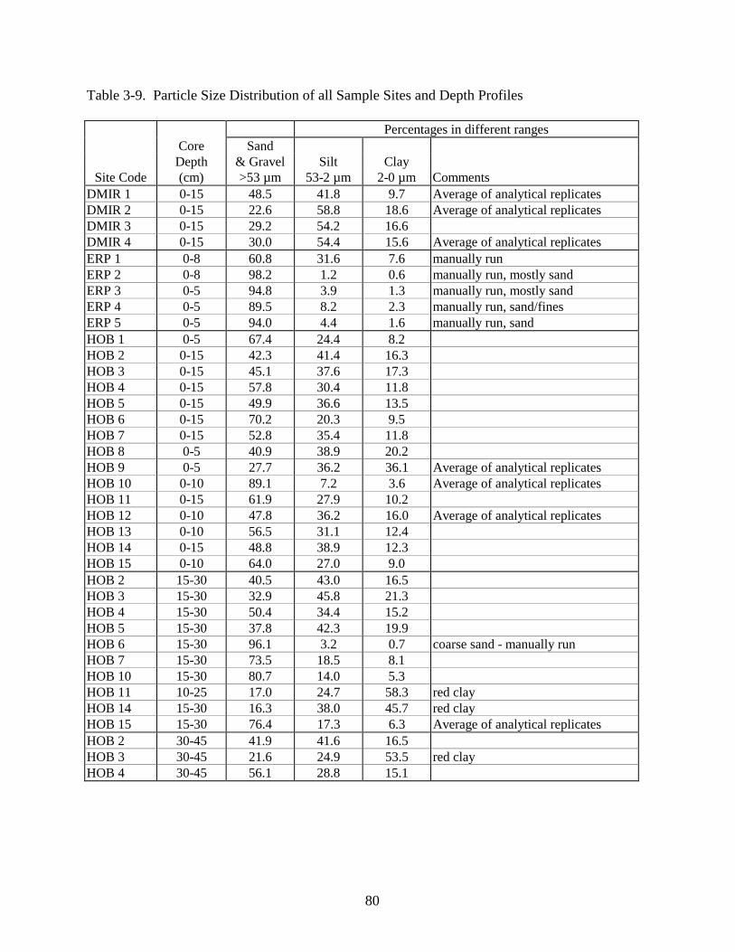
Table 3-9. Particle Size Distribution of all Sample Sites and Depth Profiles

80

Percentages in different rangesCore Sand

Depth & Gravel Silt ClaySite Code (cm) >53 µm 53-2 µm 2-0 µm Comments

DMIR 1 0-15 48.5 41.8 9.7 Average of analytical replicatesDMIR 2 0-15 22.6 58.8 18.6 Average of analytical replicatesDMIR 3 0-15 29.2 54.2 16.6DMIR 4 0-15 30.0 54.4 15.6 Average of analytical replicatesERP 1 0-8 60.8 31.6 7.6 manually runERP 2 0-8 98.2 1.2 0.6 manually run, mostly sandERP 3 0-5 94.8 3.9 1.3 manually run, mostly sandERP 4 0-5 89.5 8.2 2.3 manually run, sand/finesERP 5 0-5 94.0 4.4 1.6 manually run, sandHOB 1 0-5 67.4 24.4 8.2HOB 2 0-15 42.3 41.4 16.3HOB 3 0-15 45.1 37.6 17.3HOB 4 0-15 57.8 30.4 11.8HOB 5 0-15 49.9 36.6 13.5HOB 6 0-15 70.2 20.3 9.5HOB 7 0-15 52.8 35.4 11.8HOB 8 0-5 40.9 38.9 20.2HOB 9 0-5 27.7 36.2 36.1 Average of analytical replicatesHOB 10 0-10 89.1 7.2 3.6 Average of analytical replicatesHOB 11 0-15 61.9 27.9 10.2HOB 12 0-10 47.8 36.2 16.0 Average of analytical replicatesHOB 13 0-10 56.5 31.1 12.4HOB 14 0-15 48.8 38.9 12.3HOB 15 0-10 64.0 27.0 9.0HOB 2 15-30 40.5 43.0 16.5HOB 3 15-30 32.9 45.8 21.3HOB 4 15-30 50.4 34.4 15.2HOB 5 15-30 37.8 42.3 19.9HOB 6 15-30 96.1 3.2 0.7 coarse sand - manually runHOB 7 15-30 73.5 18.5 8.1HOB 10 15-30 80.7 14.0 5.3HOB 11 10-25 17.0 24.7 58.3 red clayHOB 14 15-30 16.3 38.0 45.7 red clayHOB 15 15-30 76.4 17.3 6.3 Average of analytical replicatesHOB 2 30-45 41.9 41.6 16.5HOB 3 30-45 21.6 24.9 53.5 red clayHOB 4 30-45 56.1 28.8 15.1

Table 3-9. Continued

81

Percentages in different rangesCore Sand

Depth & Gravel Silt ClaySite Code (cm) >53 µm 53-2 µm 2-0 µm Comments

HOB 5 30-45 51.6 34.9 13.5HOB 6 30-45 94.8 3.4 1.8 manually run, coarse sandHOB 7 30-45 61.6 27.0 11.4HOB 10 30-45 71.7 20.5 7.9HOB 11 25-40 22.3 27.4 50.3 red clayHOB 14 30-45 32.4 52.0 15.5 lots of woodHOB 15 30-45 78.9 14.8 6.2 Average of analytical replicatesKMB 1 0-8 67.5 27.0 5.4KMB 2 0-12 44.3 46.6 9.1KMB 3 0-15 38.5 46.2 15.3 wood fiberKMB 4 0-15 28.5 44.6 26.9 Average of analytical replicatesKMB 5 0-15 9.7 54.1 36.2 Average of analytical replicatesMLH 1 0-12 47.8 41.4 10.9 Average of analytical replicatesMLH 2 0-20 87.7 9.9 2.4 Average of analytical replicatesMLH 3 0-15 62.7 30.2 7.1MLH 4 0-20 34.5 47.8 17.7MLH 5 0-17 50.6 36.2 13.3MLH 6 0-21 92.2 5.8 2.0MLH 7 0-17 52.8 34.8 12.4 Average of analytical replicatesMLH 8 0-15.5 60.7 29.1 10.2MLH 9 0-20 45.2 40.6 14.3MLH 10 0-20 40.5 45.7 13.8MLH 1 25-40 48.1 42.2 9.6MLH 2 80-95 57.4 38.6 4.0 %T (transmittance) highMLH 3 37-52 - - - Insufficiant sample for analysisMLH 4 30-50 86.1 10.7 3.2MLH 5 32-47 60.6 32.0 7.5MLH 6 25-40 95.7 3.3 1.0 manually runMLH 7 72-87 89.8 8.4 1.8MLH 8 60-76 97.6 1.8 0.6 manually runMLH 9 52-79 69.6 26.5 3.9MLH 10 75-95 41.3 44.3 14.4 Average of analytical replicatesMNS 1 0-10 48.2 40.0 11.8MNS 2 0-12 59.4 33.3 7.3 Average of analytical replicatesMNS 3 0-15 54.1 35.8 10.1MNS 4 0-15 61.4 28.7 9.8 Average of analytical replicates

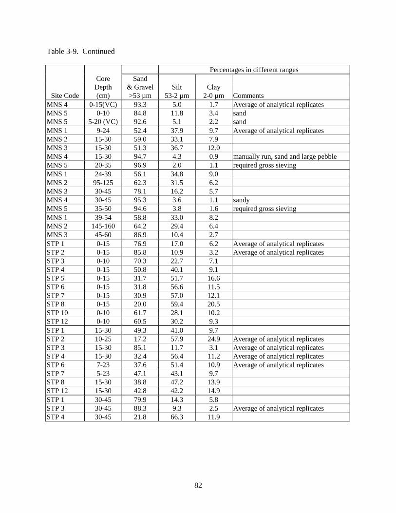
Table 3-9. Continued

82

Percentages in different rangesCore Sand

Depth & Gravel Silt ClaySite Code (cm) >53 µm 53-2 µm 2-0 µm Comments

MNS 4 0-15(VC) 93.3 5.0 1.7 Average of analytical replicatesMNS 5 0-10 84.8 11.8 3.4 sandMNS 5 5-20 (VC) 92.6 5.1 2.2 sandMNS 1 9-24 52.4 37.9 9.7 Average of analytical replicatesMNS 2 15-30 59.0 33.1 7.9MNS 3 15-30 51.3 36.7 12.0MNS 4 15-30 94.7 4.3 0.9 manually run, sand and large pebbleMNS 5 20-35 96.9 2.0 1.1 required gross sievingMNS 1 24-39 56.1 34.8 9.0MNS 2 95-125 62.3 31.5 6.2MNS 3 30-45 78.1 16.2 5.7MNS 4 30-45 95.3 3.6 1.1 sandyMNS 5 35-50 94.6 3.8 1.6 required gross sievingMNS 1 39-54 58.8 33.0 8.2MNS 2 145-160 64.2 29.4 6.4MNS 3 45-60 86.9 10.4 2.7STP 1 0-15 76.9 17.0 6.2 Average of analytical replicatesSTP 2 0-15 85.8 10.9 3.2 Average of analytical replicatesSTP 3 0-10 70.3 22.7 7.1STP 4 0-15 50.8 40.1 9.1STP 5 0-15 31.7 51.7 16.6STP 6 0-15 31.8 56.6 11.5STP 7 0-15 30.9 57.0 12.1STP 8 0-15 20.0 59.4 20.5STP 10 0-10 61.7 28.1 10.2STP 12 0-10 60.5 30.2 9.3STP 1 15-30 49.3 41.0 9.7STP 2 10-25 17.2 57.9 24.9 Average of analytical replicatesSTP 3 15-30 85.1 11.7 3.1 Average of analytical replicatesSTP 4 15-30 32.4 56.4 11.2 Average of analytical replicatesSTP 6 7-23 37.6 51.4 10.9 Average of analytical replicatesSTP 7 5-23 47.1 43.1 9.7STP 8 15-30 38.8 47.2 13.9STP 12 15-30 42.8 42.2 14.9STP 1 30-45 79.9 14.3 5.8STP 3 30-45 88.3 9.3 2.5 Average of analytical replicatesSTP 4 30-45 21.8 66.3 11.9

Table 3-9. Continued

83

Percentages in different rangesCore Sand

Depth & Gravel Silt ClaySite Code (cm) >53 µm 53-2 µm 2-0 µm Comments

STP 6 23-38 29.3 55.6 15.2STP 12 30-46 39.7 43.8 16.6 Average of analytical replicatesSTP 12 76-91 54.6 35.2 10.1 Average of analytical replicatesSUS 1 0-15 71.8 22.3 5.9SUS 2 0-15 70.6 22.6 6.8SUS 3 0-15 72.8 21.2 5.9SUS 4 0-15 67.5 26.1 6.4SUS 5 0-15 80.9 14.7 4.4SUS 6 0-15 - - - Insufficiant sample for analysisSUS 7 0-5 85.9 10.9 3.2 Average of analytical replicatesSUS 1 15-30 45.9 44.8 9.2 Average of analytical replicatesSUS 2 15-30 67.4 28.8 3.8SUS 3 15-30 83.4 13.5 3.1SUS 4 15-30 84.4 12.6 3.0SUS 5 15-23 98.2 1.4 0.4SUS 6 15-30 98.1 1.5 0.4 manually runSUS 7 15-30 91.4 7.2 1.4 manually runSUS 1 30-45 69.6 25.5 4.8SUS 2 30-45 71.6 23.6 4.8SUS 3 30-45 87.8 9.8 2.3SUS 4 30-45 77.9 18.6 3.5SUS 5 24-38 96.3 2.8 0.9 manually run, slag chunk and sandSUS 6 30-45 98.1 1.5 0.4 manually runSUS 7 30-45 99.0 0.8 0.2 manually runSUS 1 145-160 97.7 1.8 0.5 manually runSUS 2 111-126 90.9 7.4 1.8 Average of analytical replicatesSUS 3 140-155 79.8 16.9 3.3SUS 4 100-115 92.5 6.4 1.2 Average of analytical replicatesSUS 5 39-54 93.7 5.2 1.1 slag chunk in subsampleSUS 6 115-130 97.6 2.0 0.4SUS 7 63-78 99.6 0.3 0.1 manually runWLS 1 0-15 28.2 58.9 12.9 Average of analytical replicatesWLS 2 0-15 46.9 41.5 11.6 Average of analytical replicatesWLS 3 0-17 49.7 38.8 11.5WLS 4 0-20 32.9 51.5 15.6WLS 5 0-18 29.3 53.4 17.4 Average of analytical replicatesWLS 6 0-15 15.7 62.5 21.8

Table 3-9. Continued

84

Percentages in different rangesCore Sand

Depth & Gravel Silt ClaySite Code (cm) >53 µm 53-2 µm 2-0 µm Comments

WLS 7 0-15 19.1 60.1 20.8WLS 8 0-15 25.5 55.8 18.7WLS 9 0-20 16.6 64.3 19.0WLS 10 0-15 40.9 46.2 12.9WLS 11 0-20 18.2 61.4 20.4WLS 12 0-19 32.4 51.6 16.1WLS 13 0-18 37.3 45.9 16.7WLS 14 0-15 30.0 48.8 21.1WLS 15 0-5 71.0 22.1 6.9WLS 16 0-18 36.9 48.5 14.6WLS 17 0-5 82.3 14.2 3.5 Average of analytical replicatesWLS 18 0-15 50.4 38.6 11.1 Average of analytical replicatesWLS 19 0-20 31.8 49.9 18.3WLS 1 15-30 35.4 51.2 13.5WLS 2 15-30 26.6 56.2 17.2 Average of analytical replicatesWLS 3 15-30 62.2 30.9 7.0WLS 4 15-30 96.1 2.8 1.1WLS 5 15-30 38.5 45.5 16.0 sand, manually runWLS 6 15-30 46.1 40.9 13.0WLS 7 5-20 28.0 56.0 16.0WLS 8 15-30 24.7 60.4 14.9WLS 9 15-30 38.4 47.3 14.3 wood fiberWLS 10 15-30 69.6 20.2 10.3WLS 11 15-30 20.4 62.2 17.3 sandy clayWLS 12 15-30 15.6 61.6 22.9WLS 13 15-30 26.7 57.7 15.6WLS 14 15-30 55.8 36.1 8.1WLS 15 15-30 80.6 15.2 4.2WLS 16 15-30 12.8 65.7 21.5WLS 17 15-30 67.7 28.1 4.2WLS 18 15-30 43.0 43.3 13.7 Average of analytical replicatesWLS 19 15-30 31.4 50.3 18.3WLS 1 30-45 34.0 50.4 15.6WLS 2 30-45 20.5 61.0 18.5WLS 3 30-45 16.1 63.6 20.3WLS 4 30-45 97.7 1.6 0.7 manually runWLS 5 30-45 78.9 16.4 4.8 Average of analytical replicates

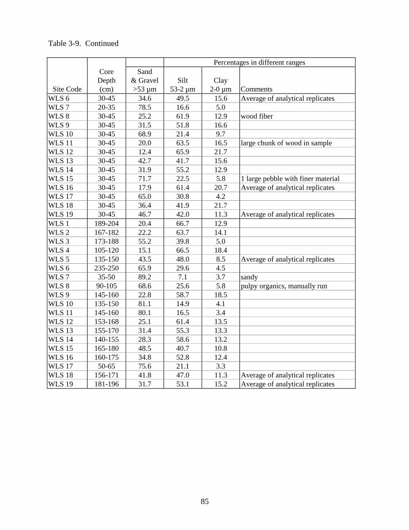
Table 3-9. Continued

85

Percentages in different rangesCore Sand

Depth & Gravel Silt ClaySite Code (cm) >53 µm 53-2 µm 2-0 µm Comments

WLS 6 30-45 34.6 49.5 15.6 Average of analytical replicatesWLS 7 20-35 78.5 16.6 5.0WLS 8 30-45 25.2 61.9 12.9 wood fiberWLS 9 30-45 31.5 51.8 16.6WLS 10 30-45 68.9 21.4 9.7WLS 11 30-45 20.0 63.5 16.5 large chunk of wood in sampleWLS 12 30-45 12.4 65.9 21.7WLS 13 30-45 42.7 41.7 15.6WLS 14 30-45 31.9 55.2 12.9WLS 15 30-45 71.7 22.5 5.8 1 large pebble with finer materialWLS 16 30-45 17.9 61.4 20.7 Average of analytical replicatesWLS 17 30-45 65.0 30.8 4.2WLS 18 30-45 36.4 41.9 21.7WLS 19 30-45 46.7 42.0 11.3 Average of analytical replicatesWLS 1 189-204 20.4 66.7 12.9WLS 2 167-182 22.2 63.7 14.1WLS 3 173-188 55.2 39.8 5.0WLS 4 105-120 15.1 66.5 18.4WLS 5 135-150 43.5 48.0 8.5 Average of analytical replicatesWLS 6 235-250 65.9 29.6 4.5WLS 7 35-50 89.2 7.1 3.7 sandyWLS 8 90-105 68.6 25.6 5.8 pulpy organics, manually runWLS 9 145-160 22.8 58.7 18.5WLS 10 135-150 81.1 14.9 4.1WLS 11 145-160 80.1 16.5 3.4WLS 12 153-168 25.1 61.4 13.5WLS 13 155-170 31.4 55.3 13.3WLS 14 140-155 28.3 58.6 13.2WLS 15 165-180 48.5 40.7 10.8WLS 16 160-175 34.8 52.8 12.4WLS 17 50-65 75.6 21.1 3.3WLS 18 156-171 41.8 47.0 11.3 Average of analytical replicatesWLS 19 181-196 31.7 53.1 15.2 Average of analytical replicates

Table 3-10. TOC Results for all Sample Sites and Depth Profiles

86

CoreDepth % Organic Replicate

Site Code (cm) Carbon % Std Dev % RSD TypeDMIR 1 0-15 2.5DMIR 2 0-15 2.3 0.02 0.93 ARDMIR 3 0-15 2.9DMIR 4 0-15 2.6ERP 1 0-8 2.9ERP 2 0-8 0.28ERP 3 0-5 2.9ERP 4 0-5 1.6 0.06 3.6 AR/ERERP 5 0-5 0.46HOB 1 0-5 1.3HOB 2 0-15 3.8HOB 3 0-15 3.5HOB 4 0-15 2.5 0.21 8.1 ERHOB 5 0-15 3.2HOB 6 0-15 2.4 0.18 7.7 ARHOB 7 0-15 3.0HOB 8 0-5 2.8HOB 9 0-5 0.90HOB 10 0-10 1.8HOB 11 0-15 3.0HOB 12 0-10 2.2HOB 13 0-10 3.2HOB 14 0-15 3.9 0.19 4.8 AR/ERHOB 15 0-10 5.2 0.49 9.5 ARHOB 2 15-30 3.7HOB 3 15-30 3.0HOB 4 15-30 3.3HOB 5 15-30 2.6HOB 6 15-30 0.66HOB 7 15-30 2.7HOB 10 15-30 3.2HOB 11 10-25 0.32HOB 14 15-30 0.92 0.02 2.3 ERHOB 15 15-30 3.7 0.01 0.19 AR

AR = Analytical replicateER = Extraction replicate

Table 3-10. Continued

87

CoreDepth % Organic Replicate

Site Code (cm) Carbon % Std Dev % RSD TypeHOB 2 30-45 4.3HOB 3 30-45 0.67HOB 4 30-45 4.1HOB 5 30-45 2.2HOB 6 30-45 0.32HOB 7 30-45 2.9HOB 10 30-45 1.9HOB 11 25-40 0.34HOB 14 30-45 4.7 0.06 1.4 ERHOB 15 30-45 4.4 0.83 19 ARKMB 1 0-8 2.2KMB 2 0-12 1.7KMB 3 0-15 3.1KMB 4 0-15 2.2 0.07 3.2 ARKMB 5 0-15 2.8MLH 1 0-12 5.0 0.01 0.14 ARMLH 2 0-20 7.1MLH 3 0-15 12MLH 4 0-20 6.6MLH 5 0-17 6.5 0.10 1.5 ARMLH 6 0-21 0.89MLH 7 0-17 3.8MLH 8 0-15.5 4.8MLH 9 0-20 6.3MLH 10 0-20 3.4 0.09 2.7 AR/ERMLH 1 25-40 2.0MLH 2 80-95 19 0.40 2.1 ARMLH 3 37-52 15 1.9 13 ARMLH 4 30-50 2.4MLH 5 32-47 2.1MLH 6 25-40 2.4MLH 7 72-87 1.3 0.19 15 ERMLH 8 60-76 0.18MLH 9 52-79 15 0.69 4.6 ARMLH 10 75-95 4.1

AR = Analytical replicateER = Extraction replicate

Table 3-10. Continued

88

CoreDepth % Organic Replicate

Site Code (cm) Carbon % Std Dev % RSD TypeMNS 1 0-10 4.0 0.01 0.35 ERMNS 2 0-12 4.8MNS 3 0-15 3.2MNS 4 0-15 3.5MNS 4 0-15(VC) 2.6MNS 5 0-10 2.4 0.01 0.58 ARMNS 5 5-20 (VC) 1.6MNS 1 9-24 3.4MNS 2 15-30 3.8MNS 3 15-30 4.6MNS 4 15-30 1.9MNS 5 20-35 0.67 0.09 14 ARMNS 1 24-39 4.2 0.02 0.50 ERMNS 2 95-125 6.7MNS 3 30-45 4.0 0.28 6.9 ARMNS 4 30-45 2.2 0.16 7.3 ERMNS 5 35-50 2.9MNS 1 39-54 4.0MNS 2 145-160 4.6MNS 3 45-60 4.1 0.59 14 ARSTP 1 0-15 3.0STP 2 0-15 3.4STP 3 0-10 3.4STP 4 0-15 3.6STP 5 0-15 4.1STP 6 0-15 3.4STP 7 0-15 3.2STP 8 0-15 5.0STP 10 0-10 3.4 0.16 4.8 ERSTP 12 0-10 4.1STP 1 15-30 4.0 0.25 6.3 ARSTP 2 10-25 4.5STP 3 15-30 3.9STP 4 15-30 3.4STP 6 7-23 3.2

AR = Analytical replicateER = Extraction replicate

Table 3-10. Continued

89

CoreDepth % Organic Replicate

Site Code (cm) Carbon % Std Dev % RSD TypeSTP 7 5-23 3.2STP 8 15-30 5.0STP 12 15-30 4.7STP 1 30-45 2.3 0.13 5.9 AR/ERSTP 3 30-45 2.0STP 3 30-45 1.8 0.03 1.6 ARSTP 4 30-45 4.6STP 6 23-38 3.6STP 12 30-46 3.7STP 12 76-91 6.4SUS 1 0-15 4.7 0.05 1.1 ARSUS 2 0-15 3.5SUS 3 0-15 4.9SUS 4 0-15 4.3SUS 5 0-15 2.3SUS 6 0-15 1.9SUS 7 0-5 2.7 0.11 4.0 ERSUS 1 15-30 19 0.91 4.9 ARSUS 2 15-30 19 0.74 3.9 ARSUS 3 15-30 4.8SUS 4 15-30 2.8SUS 5 15-23 0.83SUS 6 15-30 0.33SUS 7 15-30 3.0SUS 1 30-45 15 0.08 0.58 ARSUS 2 30-45 11SUS 3 30-45 3.6 0.01 0.40 ERSUS 4 30-45 4.3SUS 5 24-38 0.80SUS 6 30-45 0.28SUS 7 30-45 1.4

AR = Analytical replicateER = Extraction replicate

Table 3-10. Continued

90

CoreDepth % Organic Replicate

Site Code (cm) Carbon % Std Dev % RSD TypeSUS 1 145-160 1.4SUS 2 111-126 2.7SUS 3 140-155 3.1SUS 4 100-115 3.2 0.60 19 ARSUS 5 39-54 2.4SUS 6 115-130 1.1 0.07 6.7 ERSUS 7 63-78 0.29WLS 1 0-15 2.9WLS 2 0-15 2.3WLS 3 0-17 3.1WLS 4 0-20 3.0WLS 5 0-18 4.9 0.80 16 AR/ERWLS 6 0-15 3.7WLS 7 0-15 3.5WLS 8 0-15 4.5WLS 9 0-20 3.8WLS 10 0-15 1.7WLS 11 0-20 3.6WLS 12 0-19 4.9 0.05 1.0 ARWLS 13 0-18 4.7WLS 14 0-15 5.6WLS 15 0-5 2.6 0.83 32 AR/ERWLS 16 0-18 4.7WLS 17 0-5 2.8 0.11 4.1 ARWLS 18 0-15 2.7WLS 19 0-20 4.4WLS 1 15-30 3.3WLS 2 15-30 1.0WLS 3 15-30 3.5WLS 4 15-30 1.1WLS 5 15-30 8.7 0.93 11 ARWLS 6 15-30 2.8WLS 7 5-20 3.7 0.09 2.5 AR/ERWLS 8 15-30 3.9

AR = Analytical replicateER = Extraction replicate

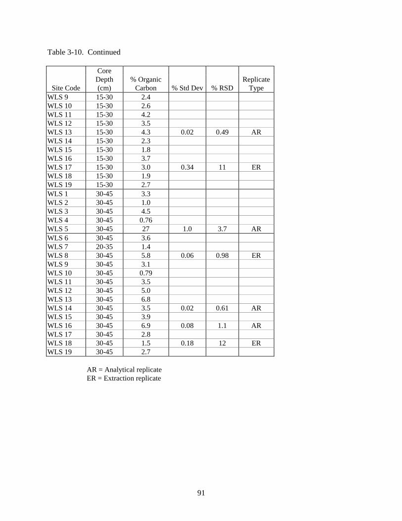
Table 3-10. Continued

91

CoreDepth % Organic Replicate

Site Code (cm) Carbon % Std Dev % RSD TypeWLS 9 15-30 2.4WLS 10 15-30 2.6WLS 11 15-30 4.2WLS 12 15-30 3.5WLS 13 15-30 4.3 0.02 0.49 ARWLS 14 15-30 2.3WLS 15 15-30 1.8WLS 16 15-30 3.7WLS 17 15-30 3.0 0.34 11 ERWLS 18 15-30 1.9WLS 19 15-30 2.7WLS 1 30-45 3.3WLS 2 30-45 1.0WLS 3 30-45 4.5WLS 4 30-45 0.76WLS 5 30-45 27 1.0 3.7 ARWLS 6 30-45 3.6WLS 7 20-35 1.4WLS 8 30-45 5.8 0.06 0.98 ERWLS 9 30-45 3.1WLS 10 30-45 0.79WLS 11 30-45 3.5WLS 12 30-45 5.0WLS 13 30-45 6.8WLS 14 30-45 3.5 0.02 0.61 ARWLS 15 30-45 3.9WLS 16 30-45 6.9 0.08 1.1 ARWLS 17 30-45 2.8WLS 18 30-45 1.5 0.18 12 ERWLS 19 30-45 2.7

AR = Analytical replicateER = Extraction replicate

Table 3-10. Continued

92

CoreDepth % Organic Replicate

Site Code (cm) Carbon % Std Dev % RSD TypeWLS 1 189-204 3.7WLS 2 167-182 5.2WLS 3 173-188 6.1WLS 4 105-120 4.3WLS 5 135-150 17 0.24 1.4 ARWLS 6 235-250 2.2 0.22 9.9 ERWLS 7 35-50 1.6WLS 8 90-105 27 0.06 0.24 ARWLS 9 145-160 3.1WLS 10 135-150 0.38WLS 11 145-160 1.7WLS 12 153-168 4.4WLS 13 155-170 3.4WLS 14 140-155 2.4WLS 15 165-180 2.6WLS 16 160-175 4.6 0.06 1.4 ERWLS 17 50-65 3.3WLS 18 156-171 1.7WLS 19 181-196 1.8

AR = Analytical replicateER = Extraction replicate

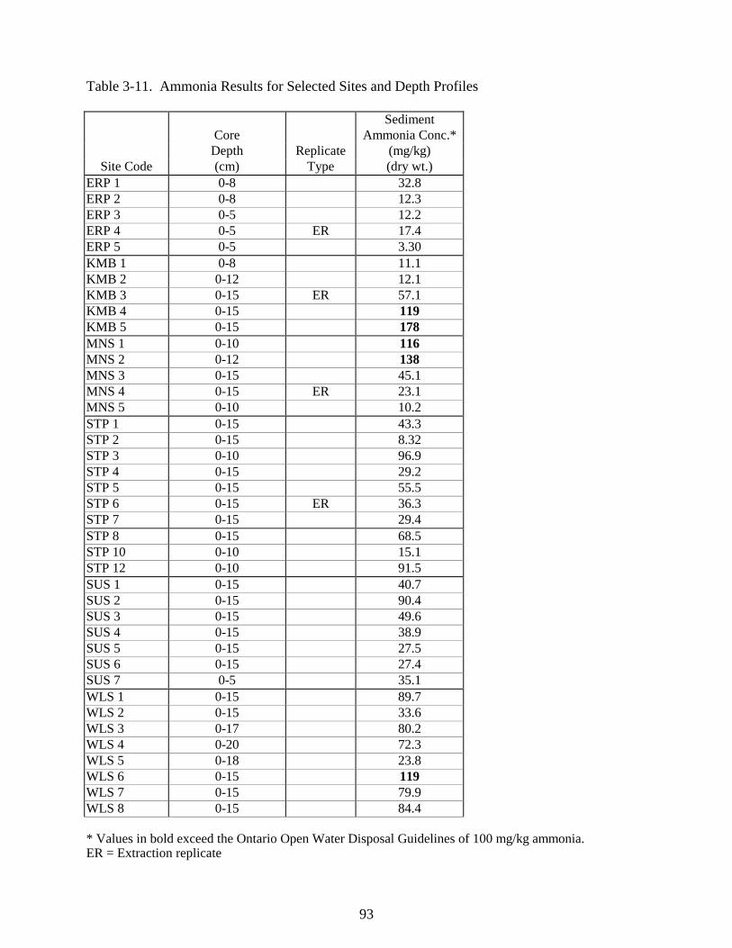
Table 3-11. Ammonia Results for Selected Sites and Depth Profiles

93

SedimentCore Ammonia Conc.*

Depth Replicate (mg/kg)Site Code (cm) Type (dry wt.)

ERP 1 0-8 32.8ERP 2 0-8 12.3ERP 3 0-5 12.2ERP 4 0-5 ER 17.4ERP 5 0-5 3.30KMB 1 0-8 11.1KMB 2 0-12 12.1KMB 3 0-15 ER 57.1KMB 4 0-15 119KMB 5 0-15 178MNS 1 0-10 116MNS 2 0-12 138MNS 3 0-15 45.1MNS 4 0-15 ER 23.1MNS 5 0-10 10.2STP 1 0-15 43.3STP 2 0-15 8.32STP 3 0-10 96.9STP 4 0-15 29.2STP 5 0-15 55.5STP 6 0-15 ER 36.3STP 7 0-15 29.4STP 8 0-15 68.5STP 10 0-10 15.1STP 12 0-10 91.5SUS 1 0-15 40.7SUS 2 0-15 90.4SUS 3 0-15 49.6SUS 4 0-15 38.9SUS 5 0-15 27.5SUS 6 0-15 27.4SUS 7 0-5 35.1WLS 1 0-15 89.7WLS 2 0-15 33.6WLS 3 0-17 80.2WLS 4 0-20 72.3WLS 5 0-18 23.8WLS 6 0-15 119WLS 7 0-15 79.9WLS 8 0-15 84.4

* Values in bold exceed the Ontario Open Water Disposal Guidelines of 100 mg/kg ammonia.ER = Extraction replicate

Table 3-11. Continued

94

SedimentCore Ammonia Conc.*

Depth Replicate (mg/kg)Site Code (cm) Type (dry wt.)

WLS 9 0-20 ER 123WLS 10 0-15 15.5WLS 11 0-20 219WLS 12 0-19 150WLS 13 0-18 101WLS 14 0-15 63.2WLS 15 0-5 24.9WLS 16 0-18 101WLS 17 0-5 ER 19.5WLS 18 0-15 21.9WLS 19 0-20 65.8WLS 1 189-204 70.4WLS 2 167-182 176WLS 3 173-188 25.9WLS 4 105-120 125WLS 5 135-150 30.5WLS 6 235-250 6.69WLS 7 35-50 NDWLS 8 90-105 183WLS 9 145-160 164WLS 10 135-150 32.3WLS 11 145-160 30.6WLS 12 153-168 104WLS 13 155-170 41.9WLS 14 140-155 97.1WLS 15 165-180 101WLS 16 160-175 ER 68.3WLS 17 50-65 52.1WLS 18 156-171 81.3WLS 19 181-196 102

*Values in bold exceed the Ontario Open Water Disposal Guidelines of 100 mg/kg ammonia.ER = Extraction replicate

Table 3-12. Total Arsenic and Lead Results for Howard’s Bay Samples

95

Total As Total PbCore Conc. Conc.Depth Replicate (mg/kg) (mg/kg)

Site Code (cm) Type (dry wt.) (dry wt.)HOB 1 0-5 ER 12.0 20.1HOB 1 0-5 (Vibr) 7.82 9.08HOB 2 0-15 23.7 111HOB 3 0-15 27.3 92.5HOB 4 0-15 16.7 78.5HOB 5 0-15 9.59 89.3HOB 6 0-15 12.9 28.1HOB 7 0-15 20.5 163HOB 8 0-5 24.3 113HOB 9 0-5 26.6 34.1HOB 10 0-10 8.21 94.5HOB 11 0-15 ER 17.7 215HOB 12 0-10 27.5 132HOB 13 0-10 19.3 269HOB 14 0-15 23.1 104HOB 15 0-10 14.2 194HOB 1 5-20 11.6 1500HOB 2 15-30 22.6 99.5HOB 3 15-30 13.0 73.1HOB 4 15-30 22.3 125HOB 5 15-30 27.0 67.3HOB 6 15-30 ER 1.40 8.17HOB 7 15-30 12.9 123HOB 10 15-30 10.3 76.2HOB 11 10-25 22.1 37.0HOB 14 15-30 35.2 67.7HOB 15 15-30 5.35 132HOB 2 30-45 13.6 182HOB 3 30-45 18.8 42.0HOB 4 30-45 10.6 1350HOB 5 30-45 ER 7.62 79.6HOB 6 30-45 0.00 10.9HOB 7 30-45 7.19 140HOB 10 30-45 3.34 61.2HOB 11 25-40 17.4 48.5HOB 14 30-45 17.7 215HOB 15 30-45 5.11 120

Vibr = Sample collected with a vibrocorerER = Extraction replicateBold values exceed the OMOEE LEL values.Bold grey cell values exceed the OMOEE SEL values.

Table 3-13. AVS Results for Selected Sites

96

Core Sulfide Conc. MeanReplicate Depth (umol/g) Sulfide Conc. Standard

Site Code Type (cm) (dry wt.) (umol/g) Deviation %RSDDMIR 1 0-15 1.02DMIR 2 0-15 7.49DMIR 2 ER 0-15 7.24 7.36 0.17 2.3DMIR 3 0-15 3.33DMIR 4 0-15 2.62ERP 1 0-8 3.23ERP 2 0-8 0.32ERP 3 0-5 0.86ERP 4 0-5 1.11ERP 5 0-5 0.13HOB 1 0-5 1.82HOB 1 0-5 (Vibr) 0.29HOB 2 0-15 3.52HOB 3 0-15 3.33HOB 4 0-15 7.96HOB 5 0-15 6.15HOB 6 0-15 1.26HOB 7 0-15 2.49HOB 8 0-5 0.36HOB 9 0-5 0.10HOB 10 0-10 3.80HOB 10 ER 0-10 3.55 3.67 0.17 4.7HOB 11 0-15 3.12HOB 12 0-10 3.92HOB 13 0-10 3.85HOB 14 0-15 3.01HOB 14 ER 0-15 3.05 3.03 0.03 0.80HOB 15 0-10 21.7HOB 1 5-20 <LODHOB 2 15-30 5.26HOB 3 15-30 0.37HOB 4 15-30 0.13HOB 5 15-30 0.18HOB 6 15-30 <LODHOB 7 15-30 0.27HOB 7 ER 15-30 0.12

Vibr = Sample collected with the vibrocorer<LOD = Sulfide level below Limit of DetectionBold Values: Sulfide level below Limit of QuantificationER = Extraction Replicate

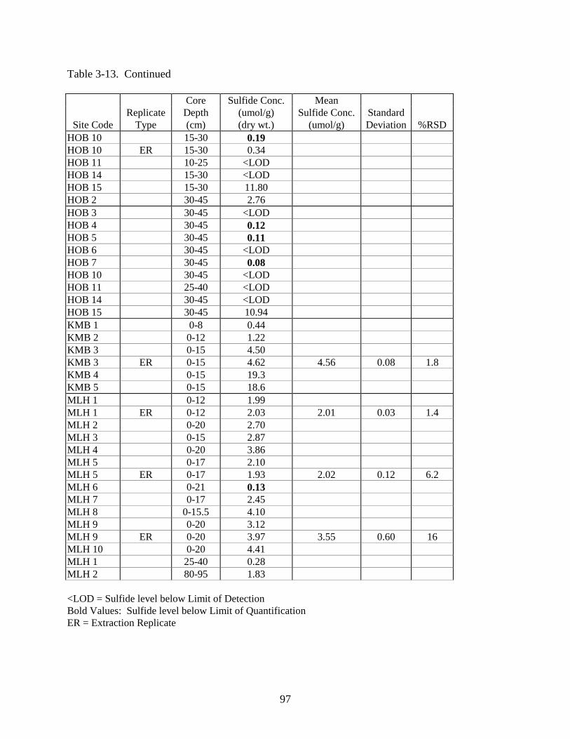
Table 3-13. Continued

97

Core Sulfide Conc. MeanReplicate Depth (umol/g) Sulfide Conc. Standard

Site Code Type (cm) (dry wt.) (umol/g) Deviation %RSDHOB 10 15-30 0.19HOB 10 ER 15-30 0.34HOB 11 10-25 <LODHOB 14 15-30 <LODHOB 15 15-30 11.80HOB 2 30-45 2.76HOB 3 30-45 <LODHOB 4 30-45 0.12HOB 5 30-45 0.11HOB 6 30-45 <LODHOB 7 30-45 0.08HOB 10 30-45 <LODHOB 11 25-40 <LODHOB 14 30-45 <LODHOB 15 30-45 10.94KMB 1 0-8 0.44KMB 2 0-12 1.22KMB 3 0-15 4.50KMB 3 ER 0-15 4.62 4.56 0.08 1.8KMB 4 0-15 19.3KMB 5 0-15 18.6MLH 1 0-12 1.99MLH 1 ER 0-12 2.03 2.01 0.03 1.4MLH 2 0-20 2.70MLH 3 0-15 2.87MLH 4 0-20 3.86MLH 5 0-17 2.10MLH 5 ER 0-17 1.93 2.02 0.12 6.2MLH 6 0-21 0.13MLH 7 0-17 2.45MLH 8 0-15.5 4.10MLH 9 0-20 3.12MLH 9 ER 0-20 3.97 3.55 0.60 16MLH 10 0-20 4.41MLH 1 25-40 0.28MLH 2 80-95 1.83

<LOD = Sulfide level below Limit of DetectionBold Values: Sulfide level below Limit of QuantificationER = Extraction Replicate

Table 3-13. Continued

98

Core Sulfide Conc. MeanReplicate Depth (umol/g) Sulfide Conc. Standard

Site Code Type (cm) (dry wt.) (umol/g) Deviation %RSDMLH 3 37-52 <LODMLH 4 30-50 0.08MLH 5 32-47 <LODMLH 6 25-40 <LODMLH 7 72-87 <LODMLH 7 ER 72-87 <LODMLH 8 60-76 <LODMLH 9 52-79 <LODMLH 10 75-95 0.18

<LOD = Sulfide level below Limit of DetectionBold Values: Sulfide level below Limit of QuantificationER = Extraction Replicate

Table 3-14. SEM Results for Selected Sites

99

Cadmium Copper Nickel Lead ZincCore Conc. Conc. Conc. Conc. Conc.

Depth Replicate (mg/kg) (mg/kg) (mg/kg) (mg/kg) (mg/kg)Site Code (cm) Type (dry wt.) (dry wt.) (dry wt.) (dry wt.) (dry wt.)

DMIR 1 0-15 0.845 13.0 7.25 20.2 64.6DMIR 2 0-15 ER 0.822 8.67 4.56 19.7 71.5DMIR 3 0-15 0.890 15.3 8.23 19.0 77.5DMIR 4 0-15 0.794 15.0 6.35 14.0 62.4ERP 1 0-8 0.741 10.8 7.00 15.8 73.3ERP 2 0-8 0.113 1.50 1.52 2.29 11.2ERP 3 0-5 0.194 2.77 4.13 4.65 20.9ERP 4 0-5 0.310 2.74 5.14 4.93 22.9ERP 5 0-5 0.144 2.31 1.88 6.14 18.3HOB 1 0-5 0.819 14.8 7.29 20.7 50.8HOB 1 0-5 (VC) 0.711 21.2 4.51 8.22 20.6HOB 2 0-15 1.23 29.9 12.8 111 145HOB 3 0-15 1.24 28.2 11.4 83.2 127HOB 4 0-15 1.05 28.6 11.8 177 119HOB 5 0-15 1.32 34.6 11.9 139 155HOB 6 0-15 0.462 11.4 6.42 47.5 33.5HOB 7 0-15 1.21 39.3 13.5 142 145HOB 8 0-5 1.17 194 14.1 97.9 151HOB 9 0-5 0.838 27.4 9.92 21.0 37.3HOB 10 0-10 ER 0.528 13.3 6.19 50.7 55.1HOB 11 0-15 1.08 40.1 12.2 277 151HOB 12 0-10 1.32 29.1 13.8 161 165HOB 13 0-10 1.51 65.3 16.6 253 177HOB 14 0-15 ER 1.01 26.7 12.3 108 112HOB 15 0-10 1.34 29.4 10.0 172 184HOB 1 5-20 0.933 3.10 2.24 <LOD 4.65HOB 2 15-30 1.54 36.9 17.7 105 169HOB 3 15-30 1.55 42.6 14.2 100 172HOB 4 15-30 1.54 44.5 14.2 139 190HOB 5 15-30 1.46 43.5 12.1 84.3 145HOB 6 15-30 0.201 1.51 2.18 0.75 6.03HOB 7 15-30 ER 0.688 18.9 4.14 111 82.5HOB 10 15-30 ER 0.606 18.8 7.19 69.4 97.1HOB 11 10-25 0.825 22.6 6.32 14.3 21.9HOB 14 15-30 1.08 23.9 7.21 92.4 75.7HOB 15 15-30 0.963 23.5 8.12 154 163

<LOD = Value obtained is lower then detection limitER = Values reported are the mean of extraction replicates

Table 3-14. Continued

100

Cadmium Copper Nickel Lead ZincCore Conc. Conc. Conc. Conc. Conc.

Depth Replicate (mg/kg) (mg/kg) (mg/kg) (mg/kg) (mg/kg)Site Code (cm) Type (dry wt.) (dry wt.) (dry wt.) (dry wt.) (dry wt.)

HOB 2 30-45 1.35 38.4 13.0 116 175HOB 3 30-45 0.962 27.0 9.84 19.1 44.5HOB 4 30-45 1.18 35.7 9.32 129 159HOB 5 30-45 1.13 27.8 8.82 63.1 108HOB 6 30-45 <LOD 1.61 1.55 4.71 4.36HOB 7 30-45 1.03 36.1 12.1 171 142HOB 10 30-45 0.676 21.7 7.18 59.3 78.0HOB 11 25-40 0.802 24.3 11.3 17.7 30.1HOB 14 30-45 0.822 29.5 11.7 234 132HOB 15 30-45 0.894 21.5 8.22 132 142KMB 1 0-8 0.419 6.92 6.81 5.47 34.0KMB 2 0-12 0.39 3.98 4.09 6.80 33.6KMB 3 0-15 ER 1.03 14.3 8.96 31.7 119KMB 4 0-15 0.973 17.6 10.6 29.6 102KMB 5 0-15 1.11 21.3 14.3 36.9 139MLH 1 0-12 1.39 15.4 8.52 30.0 78.4MLH 2 0-20 0.696 8.49 4.15 6.58 28.5MLH 3 0-15 0.975 13.7 4.73 26.4 82.0MLH 4 0-20 1.46 20.9 9.02 51.1 178MLH 5 0-17 ER 1.29 19.0 8.04 49.3 161MLH 6 0-21 0.155 3.93 2.60 3.87 14.8MLH 7 0-17 1.05 14.6 7.34 38.0 125MLH 8 0-15.5 0.949 15.9 9.08 30.3 115MLH 9 0-20 1.38 17.2 7.43 46.4 167MLH 10 0-20 0.812 9.07 6.99 17.5 81.6MLH 1 25-40 0.548 8.71 5.69 3.26 23.6MLH 2 80-95 0.545 9.91 3.43 9.69 34.7MLH 3 37-52 1.14 33.3 7.76 22.8 60.4MLH 4 30-50 0.246 5.42 4.95 1.87 18.2MLH 5 32-47 0.351 6.50 5.24 1.52 19.9MLH 6 25-40 0.175 3.51 3.52 1.40 10.8MLH 7 72-87 ER 0.250 5.18 4.01 1.51 12.7MLH 8 60-76 <LOD 4.38 3.51 0.580 8.23MLH 9 52-79 0.434 11.3 8.71 <LOD 32.5MLH 10 75-95 0.883 17.1 7.97 58.1 84.4

<LOD = Value obtained is lower then detection limitER = Values reported are the mean of extraction replicates

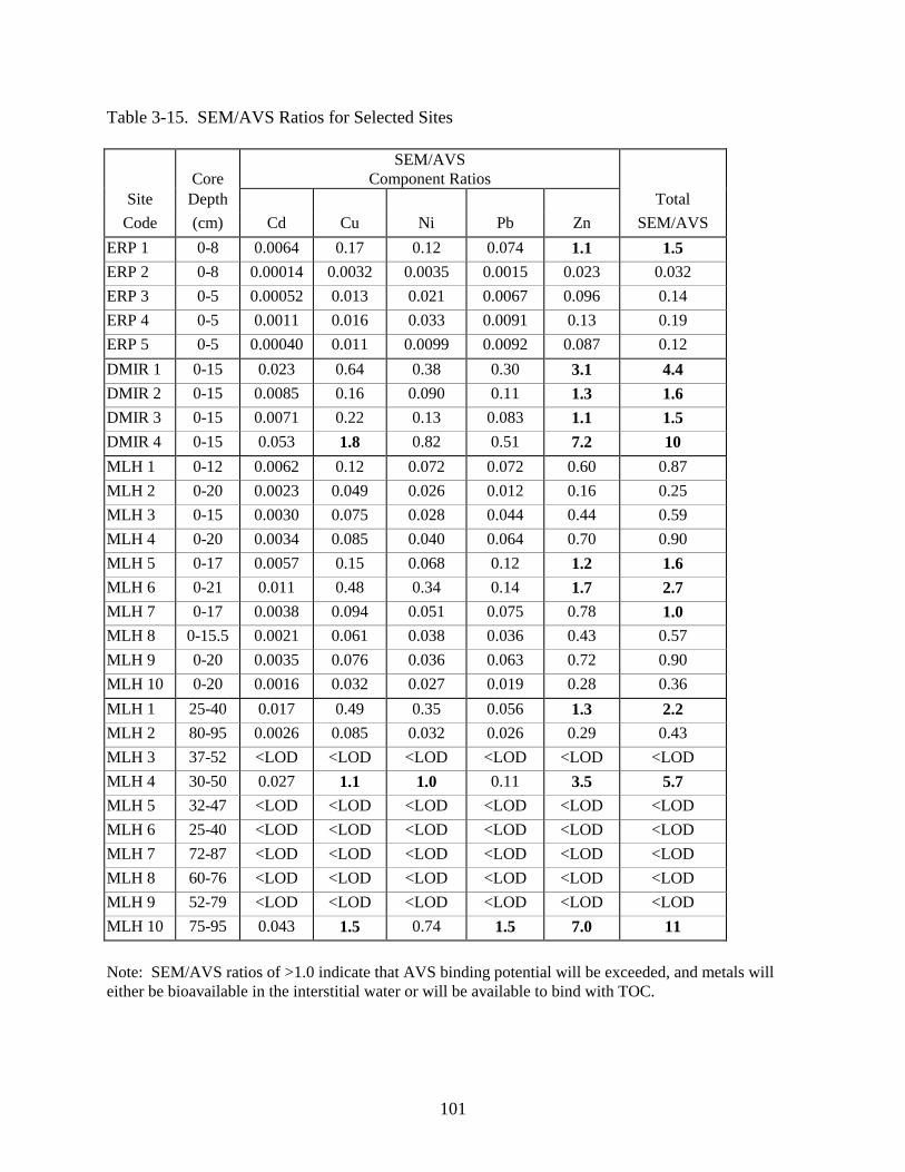
Table 3-15. SEM/AVS Ratios for Selected Sites

101

CoreSEM/AVS

Component RatiosSite Depth Total

Code (cm) Cd Cu Ni Pb Zn SEM/AVSERP 1 0-8 0.0064 0.17 0.12 0.074 1.1 1.5ERP 2 0-8 0.00014 0.0032 0.0035 0.0015 0.023 0.032ERP 3 0-5 0.00052 0.013 0.021 0.0067 0.096 0.14ERP 4 0-5 0.0011 0.016 0.033 0.0091 0.13 0.19ERP 5 0-5 0.00040 0.011 0.0099 0.0092 0.087 0.12DMIR 1 0-15 0.023 0.64 0.38 0.30 3.1 4.4DMIR 2 0-15 0.0085 0.16 0.090 0.11 1.3 1.6DMIR 3 0-15 0.0071 0.22 0.13 0.083 1.1 1.5DMIR 4 0-15 0.053 1.8 0.82 0.51 7.2 10MLH 1 0-12 0.0062 0.12 0.072 0.072 0.60 0.87MLH 2 0-20 0.0023 0.049 0.026 0.012 0.16 0.25MLH 3 0-15 0.0030 0.075 0.028 0.044 0.44 0.59MLH 4 0-20 0.0034 0.085 0.040 0.064 0.70 0.90MLH 5 0-17 0.0057 0.15 0.068 0.12 1.2 1.6MLH 6 0-21 0.011 0.48 0.34 0.14 1.7 2.7MLH 7 0-17 0.0038 0.094 0.051 0.075 0.78 1.0MLH 8 0-15.5 0.0021 0.061 0.038 0.036 0.43 0.57MLH 9 0-20 0.0035 0.076 0.036 0.063 0.72 0.90MLH 10 0-20 0.0016 0.032 0.027 0.019 0.28 0.36MLH 1 25-40 0.017 0.49 0.35 0.056 1.3 2.2MLH 2 80-95 0.0026 0.085 0.032 0.026 0.29 0.43MLH 3 37-52 <LOD <LOD <LOD <LOD <LOD <LODMLH 4 30-50 0.027 1.1 1.0 0.11 3.5 5.7MLH 5 32-47 <LOD <LOD <LOD <LOD <LOD <LODMLH 6 25-40 <LOD <LOD <LOD <LOD <LOD <LODMLH 7 72-87 <LOD <LOD <LOD <LOD <LOD <LODMLH 8 60-76 <LOD <LOD <LOD <LOD <LOD <LODMLH 9 52-79 <LOD <LOD <LOD <LOD <LOD <LODMLH 10 75-95 0.043 1.5 0.74 1.5 7.0 11

Note: SEM/AVS ratios of >1.0 indicate that AVS binding potential will be exceeded, and metals willeither be bioavailable in the interstitial water or will be available to bind with TOC.

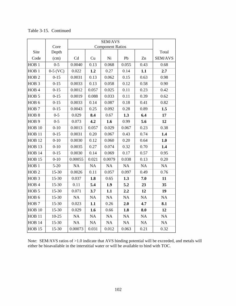
Table 3-15. Continued

102

CoreSEM/AVS

Component RatiosSite Depth Total

Code (cm) Cd Cu Ni Pb Zn SEM/AVSHOB 1 0-5 0.0040 0.13 0.068 0.055 0.43 0.68HOB 1 0-5 (VC) 0.022 1.2 0.27 0.14 1.1 2.7HOB 2 0-15 0.0031 0.13 0.062 0.15 0.63 0.98HOB 3 0-15 0.0033 0.13 0.058 0.12 0.58 0.90HOB 4 0-15 0.0012 0.057 0.025 0.11 0.23 0.42HOB 5 0-15 0.0019 0.088 0.033 0.11 0.39 0.62HOB 6 0-15 0.0033 0.14 0.087 0.18 0.41 0.82HOB 7 0-15 0.0043 0.25 0.092 0.28 0.89 1.5HOB 8 0-5 0.029 8.4 0.67 1.3 6.4 17HOB 9 0-5 0.073 4.2 1.6 0.99 5.6 12HOB 10 0-10 0.0013 0.057 0.029 0.067 0.23 0.38HOB 11 0-15 0.0031 0.20 0.067 0.43 0.74 1.4HOB 12 0-10 0.0030 0.12 0.060 0.20 0.64 1.0HOB 13 0-10 0.0035 0.27 0.074 0.32 0.70 1.4HOB 14 0-15 0.0030 0.14 0.069 0.17 0.57 0.95HOB 15 0-10 0.00055 0.021 0.0079 0.038 0.13 0.20HOB 1 5-20 NA NA NA NA NA NAHOB 2 15-30 0.0026 0.11 0.057 0.097 0.49 0.76HOB 3 15-30 0.037 1.8 0.65 1.3 7.0 11HOB 4 15-30 0.11 5.4 1.9 5.2 23 35HOB 5 15-30 0.071 3.7 1.1 2.2 12 19HOB 6 15-30 NA NA NA NA NA NAHOB 7 15-30 0.023 1.1 0.26 2.0 4.7 8.1HOB 10 15-30 0.029 1.6 0.66 1.8 8.0 12HOB 11 10-25 NA NA NA NA NA NAHOB 14 15-30 NA NA NA NA NA NAHOB 15 15-30 0.00073 0.031 0.012 0.063 0.21 0.32

Note: SEM/AVS ratios of >1.0 indicate that AVS binding potential will be exceeded, and metals willeither be bioavailable in the interstitial water or will be available to bind with TOC.

Table 3-15. Continued

103

CoreSEM/AVS

Component RatiosSite Depth Total

Code (cm) Cd Cu Ni Pb Zn SEM/AVSHOB 2 30-45 0.0044 0.22 0.08 0.20 0.97 1.5HOB 3 30-45 NA NA NA NA NA NAHOB 4 30-45 0.084 4.5 1.3 5.0 20 30HOB 5 30-45 0.089 3.9 1.3 2.7 15 23HOB 6 30-45 NA NA NA NA NA NAHOB 7 30-45 0.11 6.8 2.5 9.9 26 46HOB 10 30-45 NA NA NA NA NA NAHOB 11 25-40 NA NA NA NA NA NAHOB 14 30-45 NA NA NA NA NA NAHOB 15 30-45 0.00073 0.031 0.013 0.058 0.20 0.30KMB 1 0-8 0.0084 0.25 0.26 0.060 1.2 1.7KMB 2 0-12 0.0028 0.051 0.057 0.027 0.42 0.56KMB 3 0-15 0.0020 0.050 0.033 0.034 0.40 0.52KMB 4 0-15 0.00045 0.014 0.0093 0.0074 0.081 0.11KMB 5 0-15 0.00053 0.018 0.013 0.0096 0.11 0.16

Note: SEM/AVS ratios of >1.0 indicate that AVS binding potential will be exceeded, and metals willeither be bioavailable in the interstitial water or will be available to bind with TOC.

Table 3-16. Comparison of SEM Lead and Total Lead Concentrations in Howard’s Bay

104

SEM Pb Total Pb SEM Pb Total PbCore Conc. Conc. Core Conc. Conc.Depth (mg/kg) (mg/kg) Depth (mg/kg) (mg/kg)

Site Code (cm) (dry wt.) (dry wt.) Site Code (cm) (dry wt.) (dry wt.)HOB 1 0-5 20.7 20.1 HOB 1 5-20 <LOD 1500HOB 1 0-5 (Vibr) 8.2 9.1 HOB 2 15-30 105 99.5HOB 2 0-15 111 111 HOB 3 15-30 100 73.1HOB 3 0-15 83.2 92.5 HOB 4 15-30 139 125HOB 4 0-15 177 78.5 HOB 5 15-30 84.3 67.3HOB 5 0-15 139 89.3 HOB 6 15-30 0.75 8.17HOB 6 0-15 47.5 28.1 HOB 7 15-30 111 123HOB 7 0-15 142 163 HOB 10 15-30 69.4 76.2HOB 8 0-5 97.9 113 HOB 11 10-25 14.3 37.0HOB 9 0-5 21.0 34.1 HOB 14 15-30 92.4 67.7HOB 10 0-10 50.7 94.5 HOB 15 15-30 154 132HOB 11 0-15 277 215 mean 79.1 210HOB 12 0-10 161 132 standard deviation 53.1 430HOB 13 0-10 253 269 median 84.3 73.1HOB 14 0-15 108 104 range: low <LOD 8.17HOB 15 0-10 172 194 high 154 1500

mean 117 109standard deviation 79.6 72.8

median 108 94.5range: low 8.2 9.1

high 277 269 SEM Pb Total PbCore Conc. Conc.

Depth (mg/kg) (mg/kg)Site Code (cm) (dry wt.) (dry wt.)HOB 2 30-45 116 182HOB 3 30-45 19.1 42.0HOB 4 30-45 129 1350HOB 5 30-45 63.1 79.6HOB 6 30-45 4.7 10.9HOB 7 30-45 171 140HOB 10 30-45 59.3 61.2HOB 11 25-40 17.7 48.5HOB 14 30-45 234 215HOB 15 30-45 132 120

mean 94.6 225standard deviation 74.7 400

median 63.1 79.6range: low 4.7 10.9

high 234 1350

* LOD = Limit of Detection

Table 3-17. Mercury Results for Selected Sites and Depth Profiles

105

Mercury Mean Mercury MeanCore Conc. Mercury Core Conc. Mercury

Replicate Depth (mg/kg) (mg/kg) Replicate Depth (mg/kg) (mg/kg)Site Code Type (cm) (dry wt.) (dry wt.) Site Code Type (cm) (dry wt.) (dry wt.)HOB 1 0-5 0.088 HOB 10 15-30 0.350HOB 1 0-5 (VC) ND HOB 11 10-25 0.030HOB 2 0-15 0.490 HOB 14 15-30 NDHOB 3 ER 0-15 0.486 HOB 15 15-30 2.600HOB 3 ER 0-15 0.382 0.434** HOB 2 30-45 0.560HOB 4 0-15 0.320 HOB 3 30-45 0.061HOB 5 0-15 0.460 HOB 4 ER 30-45 0.678HOB 6 ER 0-15 0.052 HOB 4 ER 30-45 0.666 0.672**HOB 6 ER 0-15 0.552 0.302** HOB 5 30-45 0.550HOB 7 0-15 0.500 HOB 6 30-45 NDHOB 8 0-5(ponar) 0.980 HOB 7 30-45 0.500HOB 9 0-5 0.190 HOB 10 30-45 0.100HOB 10 0-10 0.210 HOB 11 25-40 0.160HOB 11 0-15 0.540 HOB 14 30-45 0.230HOB 12 0-10 0.310 HOB 15 ER 30-45 0.640HOB 13 ER 0-10 0.717 HOB 15 ER 30-45 0.654 0.647**HOB 13 ER 0-10 0.417 0.720**HOB 14 0-15 0.350HOB 15 ER 0-10 0.516HOB 15 ER 0-10 0.633HOB 15 ER 0-10 0.485HOB 15 ER 0-10 0.659 0.573**HOB 1 5-20 NDHOB 2 ER 15-30 0.506HOB 2 ER 15-30 0.440 0.473**HOB 3 ER 15-30 0.911HOB 3 ER 15-30 0.668 0.790**HOB 4 ER 15-30 0.603HOB 4 ER 15-30 0.600 0.602**HOB 5 15-30 0.760HOB 6 15-30 NDHOB 7 ER 15-30 0.242HOB 7 ER 15-30 0.207 0.224**

** = QC was exceededER = Environmental replicateBold values exceed the OMOEE LEL value of 0.2 mg/kg mercury.Bold and shaded values exceed the OMOEE SEL value of 2 mg/kg mercury.

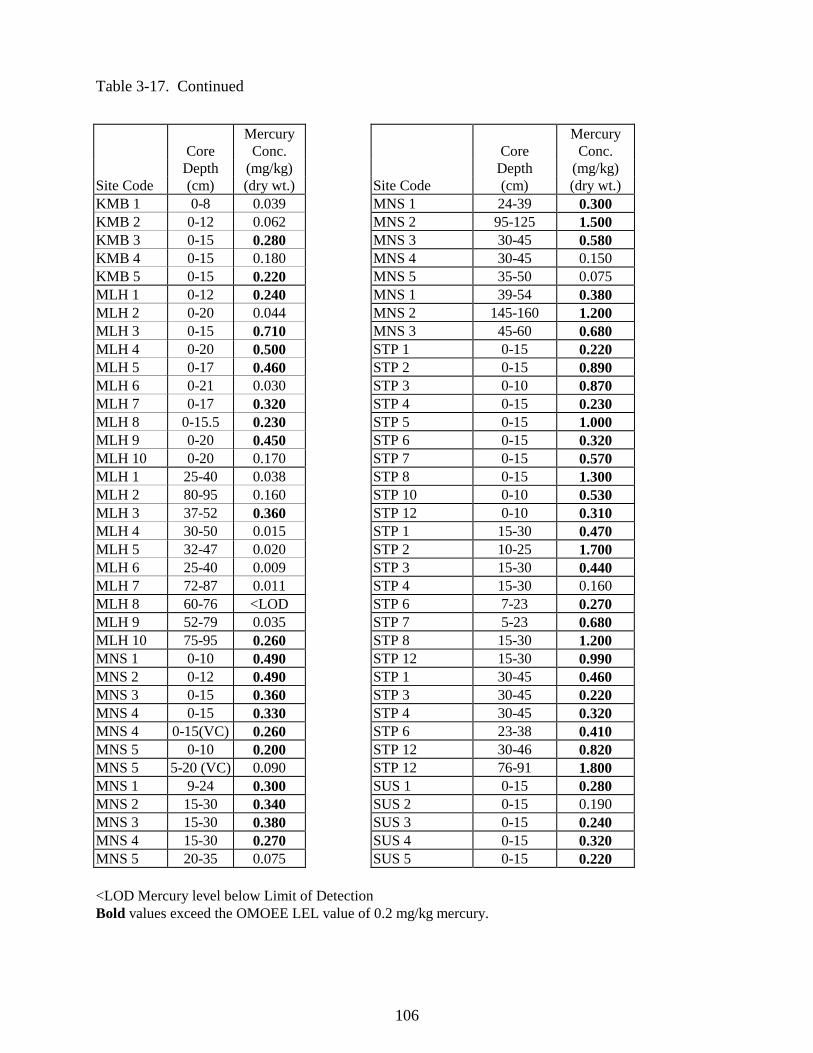
Table 3-17. Continued

106

Mercury MercuryCore Conc. Core Conc.Depth (mg/kg) Depth (mg/kg)

Site Code (cm) (dry wt.) Site Code (cm) (dry wt.)KMB 1 0-8 0.039 MNS 1 24-39 0.300KMB 2 0-12 0.062 MNS 2 95-125 1.500KMB 3 0-15 0.280 MNS 3 30-45 0.580KMB 4 0-15 0.180 MNS 4 30-45 0.150KMB 5 0-15 0.220 MNS 5 35-50 0.075MLH 1 0-12 0.240 MNS 1 39-54 0.380MLH 2 0-20 0.044 MNS 2 145-160 1.200MLH 3 0-15 0.710 MNS 3 45-60 0.680MLH 4 0-20 0.500 STP 1 0-15 0.220MLH 5 0-17 0.460 STP 2 0-15 0.890MLH 6 0-21 0.030 STP 3 0-10 0.870MLH 7 0-17 0.320 STP 4 0-15 0.230MLH 8 0-15.5 0.230 STP 5 0-15 1.000MLH 9 0-20 0.450 STP 6 0-15 0.320MLH 10 0-20 0.170 STP 7 0-15 0.570MLH 1 25-40 0.038 STP 8 0-15 1.300MLH 2 80-95 0.160 STP 10 0-10 0.530MLH 3 37-52 0.360 STP 12 0-10 0.310MLH 4 30-50 0.015 STP 1 15-30 0.470MLH 5 32-47 0.020 STP 2 10-25 1.700MLH 6 25-40 0.009 STP 3 15-30 0.440MLH 7 72-87 0.011 STP 4 15-30 0.160MLH 8 60-76 <LOD STP 6 7-23 0.270MLH 9 52-79 0.035 STP 7 5-23 0.680MLH 10 75-95 0.260 STP 8 15-30 1.200MNS 1 0-10 0.490 STP 12 15-30 0.990MNS 2 0-12 0.490 STP 1 30-45 0.460MNS 3 0-15 0.360 STP 3 30-45 0.220MNS 4 0-15 0.330 STP 4 30-45 0.320MNS 4 0-15(VC) 0.260 STP 6 23-38 0.410MNS 5 0-10 0.200 STP 12 30-46 0.820MNS 5 5-20 (VC) 0.090 STP 12 76-91 1.800MNS 1 9-24 0.300 SUS 1 0-15 0.280MNS 2 15-30 0.340 SUS 2 0-15 0.190MNS 3 15-30 0.380 SUS 3 0-15 0.240MNS 4 15-30 0.270 SUS 4 0-15 0.320MNS 5 20-35 0.075 SUS 5 0-15 0.220

<LOD Mercury level below Limit of DetectionBold values exceed the OMOEE LEL value of 0.2 mg/kg mercury.

Table 3-17. Continued

107

Mercury MercuryCore Conc. Core Conc.

Depth (mg/kg) Depth (mg/kg)Site Code (cm) (dry wt.) Site Code (cm) (dry wt.)SUS 6 0-15 0.260 WLS 16 0-18 0.920SUS 7 0-5 0.160 WLS 17 0-5 0.230SUS 1 15-30 0.370 WLS 18 0-15 0.170SUS 2 15-30 0.470 WLS 19 0-20 0.810SUS 3 15-30 0.600 WLS 1 15-30 0.320SUS 4 15-30 0.270 WLS 2 15-30 0.029SUS 5 15-23 0.043 WLS 3 15-30 0.290SUS 6 15-30 0.047 WLS 4 15-30 0.030SUS 7 15-30 0.270 WLS 5 15-30 1.700SUS 1 30-45 0.490 WLS 6 15-30 0.480SUS 2 30-45 0.970 WLS 7 5-20 0.900SUS 3 30-45 0.490 WLS 8 15-30 0.072SUS 4 30-45 0.240 WLS 9 15-30 0.400SUS 5 24-38 0.064 WLS 10 15-30 0.049SUS 6 30-45 0.028 WLS 11 15-30 1.300SUS 7 30-45 0.240 WLS 12 15-30 0.260SUS 1 145-160 0.170 WLS 13 15-30 2.900SUS 2 111-126 0.180 WLS 14 15-30 0.040SUS 3 140-155 0.089 WLS 15 15-30 0.046SUS 4 100-115 0.590 WLS 16 15-30 0.980SUS 5 39-54 0.170 WLS 17 15-30 0.140SUS 6 115-130 0.120 WLS 18 15-30 0.280SUS 7 63-78 0.031 WLS 19 15-30 0.400WLS 1 0-15 0.260 WLS 1 30-45 0.410WLS 2 0-15 0.260 WLS 2 30-45 0.018WLS 3 0-17 0.360 WLS 3 30-45 1.000WLS 4 0-20 0.540 WLS 4 30-45 0.040WLS 5 0-18 0.760 WLS 5 30-45 0.100WLS 6 0-15 0.520 WLS 6 30-45 0.520WLS 7 0-15 0.600 WLS 7 20-35 0.310WLS 8 0-15 1.500 WLS 8 30-45 0.082WLS 9 0-20 0.720 WLS 9 30-45 0.660WLS 10 0-15 0.260 WLS 10 30-45 0.047WLS 11 0-20 0.550 WLS 11 30-45 0.760WLS 12 0-19 0.750 WLS 12 30-45 3.900WLS 13 0-18 0.790 WLS 13 30-45 0.760WLS 14 0-15 0.720 WLS 14 30-45 0.057WLS 15 0-5 0.470 WLS 15 30-45 0.042

Bold values exceed the OMOEE LEL value of 0.2 mg/kg mercury.Bold and shaded values exceed the OMOEE SEL value of 2 mg/kg mercury.

Table 3-17. Continued

108

MercuryCore Conc.

Depth (mg/kg)Site Code (cm) (dry wt.)WLS 16 30-45 3.400WLS 17 30-45 0.140WLS 18 30-45 0.037WLS 19 30-45 0.056WLS 1 189-204 0.210WLS 2 167-182 0.140WLS 3 173-188 0.038WLS 4 105-120 0.047WLS 5 135-150 0.088WLS 6 235-250 0.160WLS 7 35-50 0.210WLS 8 90-105 0.042WLS 9 145-160 0.870WLS 10 135-150 0.029WLS 11 145-160 0.190WLS 12 153-168 0.046WLS 13 155-170 0.030WLS 14 140-155 0.035WLS 15 165-180 0.280WLS 16 160-175 0.050WLS 17 50-65 0.088WLS 18 156-171 0.024WLS 19 181-196 0.027

Bold values exceed the OMOEE LEL value of 0.2 mg/kg mercury.Bold and shaded values exceed the OMOEE SEL value of 2 mg/kg mercury.

Table 3-18. TCDD and TCDF Results for WLS and KMB Samples

109

Core TCDD TCDFSite Depth Replicate TCDD Detection TCDF Detection

Code (cm) Type (pg/g) Limit(pg/g)

(pg/g) Limit(pg/g)

WLS 1* 0-15 No Result - No Result -WLS 2* 0-15 No Result - No Result -WLS 3 0-17 7.1 - NQ 20WLS 4** 0-20 6.4 - 16 -WLS 5 0-18 ND 14 22 -WLS 6* 0-15 No Result - No Result -WLS 7** 0-15 4.4 - 28 -WLS 8* 0-15 No Result - No Result -WLS 9** 0-20 ND 1.8 40 -WLS 10 0-15 ND 4.1 NQ 13WLS 11 0-20 7.7 - 8.4 -WLS 12 0-19 3.4 - 6.4 -WLS 13 0-18 ND 3.3 5.7 -WLS 14 0-15 ND 6.8 NQ 7.0WLS 15 0-5 ND 2.9 5.8 -WLS 16 0-18 ND 6.5 9.5 -WLS 17 0-5 ND 7.2 NQ 7.0WLS 18 0-15 ND 2.9 7.5 -WLS 18 0-15 AR ND 4.0 5.5 -WLS 19 0-20 ND 1.5 12 -WLS 1 15-30 3.4 - 5.3 -WLS 2 15-30 ND 1.5 ND 0.2WLS 3 15-30 NQ 3.3 0.9 -WLS 4 15-30 ND 3.7 ND 0.4WLS 5 15-30 5.3 - 9.3 -WLS 6 15-30 22 - 34 -WLS 7 5-20 5.4 - 21 -WLS 8 15-30 ND 2.4 ND 2.2WLS 8 15-30 AR ND 4.2 ND 0.3WLS 10 15-30 ND 3.0 0.7 -WLS 11 15-30 12 - 37 -

AR = Analytical Replicate; ND = Not Detected; NQ = Not Quantifiable* No result due to 0% surrogate recovery** Surrogate recoveries outside of acceptable QA limits

Table 3-18. Continued

110

Core TCDD TCDFSite Depth Replicate TCDD Detection TCDF Detection

Code (cm) Type (pg/g) Limit (pg/g) (pg/g) Limit (pg/g)WLS 12 15-30 ND 6.9 ND 1.1WLS 13 15-30 6.8 - 12.3 -WLS 14 15-30 ND 9.6 ND 0.5WLS 15 15-30 ND 1.7 ND 0.2WLS 16 15-30 3.7 - NQ 8.1WLS 17 15-30 ND 3.0 NQ 1.7WLS 17 15-30 AR ND 2.9 NQ 3.5WLS 18 15-30 ND 4.7 ND 0.6WLS 19 15-30 ND 3.0 ND 0.5KMB 1 0-8 ND 5.3 NQ 1.6KMB 2 0-12 ND 1.5 NQ 2.7KMB 3 0-15 ND 4.6 NQ 13KMB 4 0-15 ND 2.1 NQ 5.1KMB 5 0-15 ND 1.6 NQ 9.1KMB 5 0-15 AR ND 2.8 NQ 8.8

AR = Analytical Replicate; ND = Not Detected; NQ = Not Quantifiable

Table 3-19. Screening PAH Results for Selected Sites

111

Screening ScreeningCore PAH Conc. Core PAH Conc.Depth (µg/kg) Depth (µg/kg)

Site Code (cm) (dry wt.) Site Code (cm) (dry wt.)KMB 1 0-8 2,400 MNS 1 9-24 1,200KMB 2 0-12 15,300 MNS 2 15-30 4,700KMB 3 0-15 37,400 MNS 3 15-30 1,600KMB 4 0-15 8,900 MNS 4 15-30 223,000KMB 5 0-15 4,300 MNS 5 20-35 41,000MLH 1 0-12 53,400 MNS 1 24-39 1,000MLH 2 0-20 7,000 MNS 2 95-125 3,700MLH 3 0-15 18,200 MNS 3 30-45 1,800MLH 4 0-20 52,700 MNS 4 30-45 404,000MLH 5 0-17 47,100 MNS 5 35-50 6,000MLH 6 0-21 9,200 MNS 1 39-54 2,400MLH 7 0-17 107,000 MNS 2 145-160 2,300MLH 8 0-15.5 32,400 MNS 3 45-60 6,600MLH 9 0-20 142,000 SUS 1 0-15 5,800MLH 10 0-20 33,900 SUS 2 0-15 317,000MLH 1 25-40 900 SUS 3 0-15 7,100MLH 2 80-95 2,900 SUS 4 0-15 228,000MLH 3 37-52 24,200 SUS 5 0-15 135,000MLH 4 30-50 1,800 SUS 6 0-15 223,000MLH 5 32-47 1,200 SUS 7 0-5 140,000MLH 6 25-40 1,600 SUS 1 15-30 900MLH 7 72-87 1,100 SUS 2 15-30 1,600MLH 8 60-76 < 700 SUS 3 15-30 2,900MLH 9 52-79 7,100 SUS 4 15-30 216,000MLH 10 75-95 56,000 SUS 5 15-23 240,900MNS 1 0-10 2,800 SUS 6 15-30 39,500MNS 2 0-12 2,800 SUS 7 15-30 84,500MNS 3 0-15 2,900 SUS 1 30-45 1,000MNS 4 0-15 6,900 SUS 2 30-45 900MNS 4 0-15(VC) 7,000 SUS 3 30-45 375,000MNS 5 0-10 337,000 SUS 4 30-45 6,200MNS 5 5-20 (VC) 3,800 SUS 5 24-38 83,600

Limit of Quantitation (LOQ) = 2,000 µg/Kg.Values entered in bold are greater than the limit of detection (LOD), but less than the LOQ.

Table 3-19. Continued

112

Screening ScreeningCore PAH Conc. Core PAH Conc.Depth (µg/kg) Depth (µg/kg)

Site Code (cm) (dry wt.) Site Code (cm) (dry wt.)SUS 6 30-45 34,900 WLS 9 15-30 49,500SUS 7 30-45 88,200 WLS 10 15-30 1,400SUS 1 145-160 78,000 WLS 11 15-30 145,000SUS 2 111-126 5,800 WLS 12 15-30 30,600SUS 3 140-155 37,100 WLS 13 15-30 191,000SUS 4 100-115 457,000 WLS 14 15-30 900SUS 5 39-54 155,000 WLS 15 15-30 4,100SUS 6 115-130 93,900 WLS 16 15-30 96,600SUS 7 63-78 14,800 WLS 17 15-30 21,400WLS 1 0-15 48,600 WLS 18 15-30 900WLS 2 0-15 16,900 WLS 19 15-30 10,700WLS 3 0-17 222,000 WLS 1 30-45 574,000WLS 4 0-20 3,500 WLS 2 30-45 900WLS 5 0-18 83,000 WLS 3 30-45 134,000WLS 6 0-15 23,400 WLS 4 30-45 8,300WLS 7 0-15 74,300 WLS 5 30-45 9,000WLS 8 0-15 411,000 WLS 6 30-45 150,000WLS 9 0-20 37,200 WLS 7 20-35 122,000WLS 10 0-15 18,200 WLS 8 30-45 1,200WLS 11 0-20 40,000 WLS 9 30-45 146,000WLS 12 0-19 23,100 WLS 10 30-45 3,300WLS 13 0-18 52,400 WLS 11 30-45 141,000WLS 14 0-15 34,700 WLS 12 30-45 172,000WLS 15 0-5 32,400 WLS 13 30-45 135,000WLS 16 0-18 133,000 WLS 14 30-45 900WLS 17 0-5 44,200 WLS 15 30-45 4,800WLS 18 0-15 224,000 WLS 16 30-45 370,000WLS 19 0-20 48,100 WLS 17 30-45 146,000WLS 1 15-30 14,600 WLS 18 30-45 700WLS 2 15-30 4,200 WLS 19 30-45 28,900WLS 3 15-30 55,900 WLS 1 189-204 19,000WLS 4 15-30 17,500 WLS 2 167-182 15,600WLS 5 15-30 65,300 WLS 3 173-188 1,300WLS 6 15-30 87,100 WLS 4 105-120 1,900WLS 7 5-20 188,000 WLS 5 135-150 27,900WLS 8 15-30 800 WLS 6 235-250 21,000

Limit of Quantitation (LOQ) = 2,000 µg/Kg.Values entered in bold are greater than the limit of detection (LOD), but less than the LOQ.

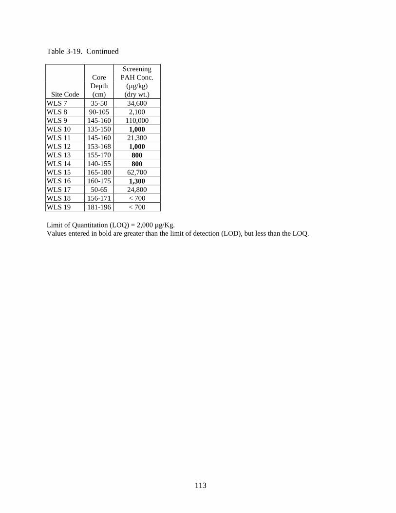
Table 3-19. Continued

113

ScreeningCore PAH Conc.Depth (µg/kg)

Site Code (cm) (dry wt.)WLS 7 35-50 34,600WLS 8 90-105 2,100WLS 9 145-160 110,000WLS 10 135-150 1,000WLS 11 145-160 21,300WLS 12 153-168 1,000WLS 13 155-170 800WLS 14 140-155 800WLS 15 165-180 62,700WLS 16 160-175 1,300WLS 17 50-65 24,800WLS 18 156-171 < 700WLS 19 181-196 < 700

Limit of Quantitation (LOQ) = 2,000 µg/Kg.Values entered in bold are greater than the limit of detection (LOD), but less than the LOQ.

Table 3-20. PAH Results (by GC/MS) for Selected Sites

114

SiteCoreDepth

PAHs (µg/kg dry wt.)

Code (cm) Acene Aceny Anth Bena Benap Benb Beng Benk Chry Diben Fluo Flut Indp Naph Phen Pyrn TotalKMB

1-C 0-8 1 3 9 41 46 75 27 21 40 8 4 52 27 12 17 46 4302-C 0-12 3 8 16 98 100 160 19 33 97 13 7 130 42 28 32 120 9003-D 0-15 < 31 < 31 60 320 290 360 85 140 320 54 41 440 160 150 130 370 3,0004-D 0-15 < 30 < 30 31 200 210 240 160 110 210 37 < 30 280 120 80 90 230 2,0005-D 0-15 < 39 < 39 57 360 390 420 480 180 380 66 41 480 210 91 150 380 3,700

MLH1-D 0-12 <26 38 100 260 210 350 120 110 340 28 43 670 94 130 330 580 3,4002-C 0-20 10 26 14 28 20 35 11 12 33 <11 22 98 <11 130 70 71 5903-D 0-15 25 70 100 270 230 330 100 98 330 33 59 640 110 430 300 480 3,6004-D 0-20 <67 220 310 1,000 940 1,300 420 420 1,100 130 160 1,900 400 1,300 650 1,500 12,0005-D 0-17 <69 170 220 780 750 1,000 430 400 830 110 130 1,400 330 850 550 1,200 9,2006-C 0-21 3 17 26 84 71 110 41 28 93 12 11 160 31 63 55 130 9407-C 0-17 26 160 290 1,100 1,300 1,600 710 600 1,100 170 100 1,800 680 660 460 1,500 12,0008-D 0-15.5 27 80 140 450 440 610 280 230 570 61 59 1,100 220 240 420 870 5,8009-D 0-20 <68 200 350 1,200 1,100 1,400 510 480 1,300 150 150 2,200 400 900 690 1,700 13,000

10-D 0-20 63 49 170 420 460 600 310 250 520 69 91 860 260 350 390 690 5,600Lowest Effect Level NA NA 220 320 370 NA 170 240 340 60 190 750 200 NA 560 490 4,000

Bold values exceed OMOEE LEL values.NA = Not applicable.C = Results merged from two separate sample runs.D = Analysis at a secondary dilution factor.Full name of PAH codes at end of Table.

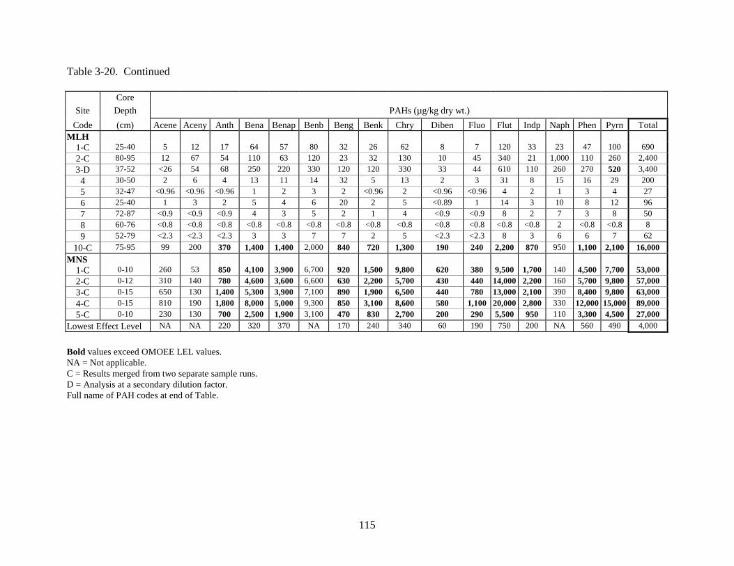
Table 3-20. Continued

115

CoreSite Depth PAHs (µg/kg dry wt.)

Code (cm) Acene Aceny Anth Bena Benap Benb Beng Benk Chry Diben Fluo Flut Indp Naph Phen Pyrn TotalMLH

1-C 25-40 5 12 17 64 57 80 32 26 62 8 7 120 33 23 47 100 6902-C 80-95 12 67 54 110 63 120 23 32 130 10 45 340 21 1,000 110 260 2,4003-D 37-52 <26 54 68 250 220 330 120 120 330 33 44 610 110 260 270 520 3,400

4 30-50 2 6 4 13 11 14 32 5 13 2 3 31 8 15 16 29 2005 32-47 <0.96 <0.96 <0.96 1 2 3 2 <0.96 2 <0.96 <0.96 4 2 1 3 4 276 25-40 1 3 2 5 4 6 20 2 5 <0.89 1 14 3 10 8 12 967 72-87 <0.9 <0.9 <0.9 4 3 5 2 1 4 <0.9 <0.9 8 2 7 3 8 508 60-76 <0.8 <0.8 <0.8 <0.8 <0.8 <0.8 <0.8 <0.8 <0.8 <0.8 <0.8 <0.8 <0.8 2 <0.8 <0.8 89 52-79 <2.3 <2.3 <2.3 3 3 7 7 2 5 <2.3 <2.3 8 3 6 6 7 62

10-C 75-95 99 200 370 1,400 1,400 2,000 840 720 1,300 190 240 2,200 870 950 1,100 2,100 16,000MNS

1-C 0-10 260 53 850 4,100 3,900 6,700 920 1,500 9,800 620 380 9,500 1,700 140 4,500 7,700 53,0002-C 0-12 310 140 780 4,600 3,600 6,600 630 2,200 5,700 430 440 14,000 2,200 160 5,700 9,800 57,0003-C 0-15 650 130 1,400 5,300 3,900 7,100 890 1,900 6,500 440 780 13,000 2,100 390 8,400 9,800 63,0004-C 0-15 810 190 1,800 8,000 5,000 9,300 850 3,100 8,600 580 1,100 20,000 2,800 330 12,000 15,000 89,0005-C 0-10 230 130 700 2,500 1,900 3,100 470 830 2,700 200 290 5,500 950 110 3,300 4,500 27,000

Lowest Effect Level NA NA 220 320 370 NA 170 240 340 60 190 750 200 NA 560 490 4,000

Bold values exceed OMOEE LEL values.NA = Not applicable.C = Results merged from two separate sample runs.D = Analysis at a secondary dilution factor.Full name of PAH codes at end of Table.

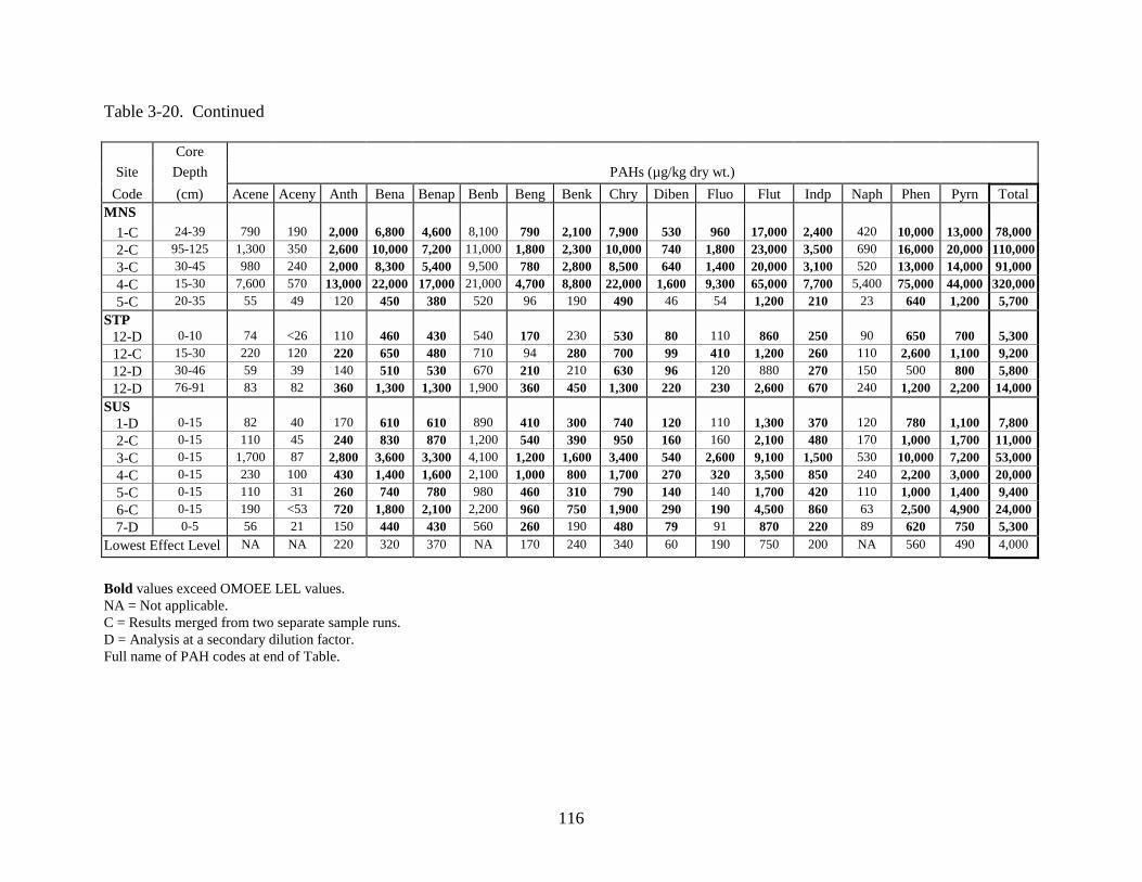
Table 3-20. Continued

116

CoreSite Depth PAHs (µg/kg dry wt.)

Code (cm) Acene Aceny Anth Bena Benap Benb Beng Benk Chry Diben Fluo Flut Indp Naph Phen Pyrn TotalMNS

1-C 24-39 790 190 2,000 6,800 4,600 8,100 790 2,100 7,900 530 960 17,000 2,400 420 10,000 13,000 78,0002-C 95-125 1,300 350 2,600 10,000 7,200 11,000 1,800 2,300 10,000 740 1,800 23,000 3,500 690 16,000 20,000 110,0003-C 30-45 980 240 2,000 8,300 5,400 9,500 780 2,800 8,500 640 1,400 20,000 3,100 520 13,000 14,000 91,0004-C 15-30 7,600 570 13,000 22,000 17,000 21,000 4,700 8,800 22,000 1,600 9,300 65,000 7,700 5,400 75,000 44,000 320,0005-C 20-35 55 49 120 450 380 520 96 190 490 46 54 1,200 210 23 640 1,200 5,700

STP12-D 0-10 74 <26 110 460 430 540 170 230 530 80 110 860 250 90 650 700 5,30012-C 15-30 220 120 220 650 480 710 94 280 700 99 410 1,200 260 110 2,600 1,100 9,20012-D 30-46 59 39 140 510 530 670 210 210 630 96 120 880 270 150 500 800 5,80012-D 76-91 83 82 360 1,300 1,300 1,900 360 450 1,300 220 230 2,600 670 240 1,200 2,200 14,000

SUS1-D 0-15 82 40 170 610 610 890 410 300 740 120 110 1,300 370 120 780 1,100 7,8002-C 0-15 110 45 240 830 870 1,200 540 390 950 160 160 2,100 480 170 1,000 1,700 11,0003-C 0-15 1,700 87 2,800 3,600 3,300 4,100 1,200 1,600 3,400 540 2,600 9,100 1,500 530 10,000 7,200 53,0004-C 0-15 230 100 430 1,400 1,600 2,100 1,000 800 1,700 270 320 3,500 850 240 2,200 3,000 20,0005-C 0-15 110 31 260 740 780 980 460 310 790 140 140 1,700 420 110 1,000 1,400 9,4006-C 0-15 190 <53 720 1,800 2,100 2,200 960 750 1,900 290 190 4,500 860 63 2,500 4,900 24,0007-D 0-5 56 21 150 440 430 560 260 190 480 79 91 870 220 89 620 750 5,300

Lowest Effect Level NA NA 220 320 370 NA 170 240 340 60 190 750 200 NA 560 490 4,000

Bold values exceed OMOEE LEL values.NA = Not applicable.C = Results merged from two separate sample runs.D = Analysis at a secondary dilution factor.Full name of PAH codes at end of Table.

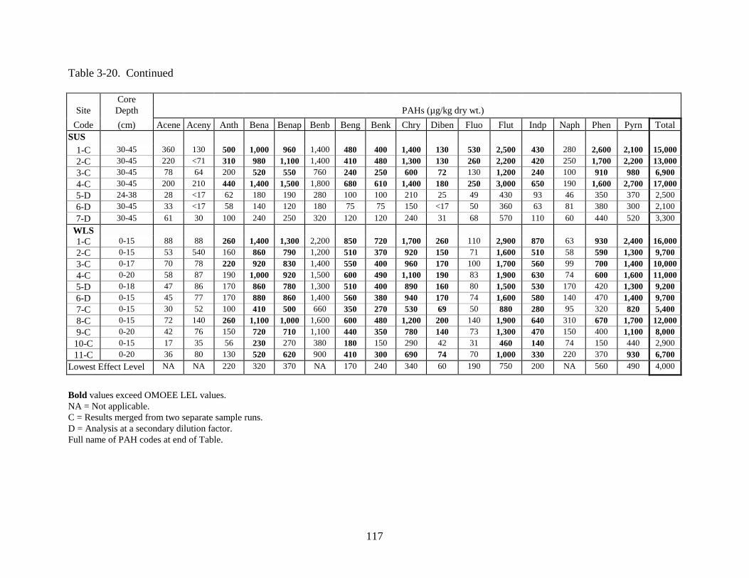
Table 3-20. Continued

117

CoreSite Depth PAHs (µg/kg dry wt.)

Code (cm) Acene Aceny Anth Bena Benap Benb Beng Benk Chry Diben Fluo Flut Indp Naph Phen Pyrn TotalSUS

1-C 30-45 360 130 500 1,000 960 1,400 480 400 1,400 130 530 2,500 430 280 2,600 2,100 15,0002-C 30-45 220 <71 310 980 1,100 1,400 410 480 1,300 130 260 2,200 420 250 1,700 2,200 13,0003-C 30-45 78 64 200 520 550 760 240 250 600 72 130 1,200 240 100 910 980 6,9004-C 30-45 200 210 440 1,400 1,500 1,800 680 610 1,400 180 250 3,000 650 190 1,600 2,700 17,0005-D 24-38 28 <17 62 180 190 280 100 100 210 25 49 430 93 46 350 370 2,5006-D 30-45 33 <17 58 140 120 180 75 75 150 <17 50 360 63 81 380 300 2,1007-D 30-45 61 30 100 240 250 320 120 120 240 31 68 570 110 60 440 520 3,300

WLS1-C 0-15 88 88 260 1,400 1,300 2,200 850 720 1,700 260 110 2,900 870 63 930 2,400 16,0002-C 0-15 53 540 160 860 790 1,200 510 370 920 150 71 1,600 510 58 590 1,300 9,7003-C 0-17 70 78 220 920 830 1,400 550 400 960 170 100 1,700 560 99 700 1,400 10,0004-C 0-20 58 87 190 1,000 920 1,500 600 490 1,100 190 83 1,900 630 74 600 1,600 11,0005-D 0-18 47 86 170 860 780 1,300 510 400 890 160 80 1,500 530 170 420 1,300 9,2006-D 0-15 45 77 170 880 860 1,400 560 380 940 170 74 1,600 580 140 470 1,400 9,7007-C 0-15 30 52 100 410 500 660 350 270 530 69 50 880 280 95 320 820 5,4008-C 0-15 72 140 260 1,100 1,000 1,600 600 480 1,200 200 140 1,900 640 310 670 1,700 12,0009-C 0-20 42 76 150 720 710 1,100 440 350 780 140 73 1,300 470 150 400 1,100 8,000

10-C 0-15 17 35 56 230 270 380 180 150 290 42 31 460 140 74 150 440 2,90011-C 0-20 36 80 130 520 620 900 410 300 690 74 70 1,000 330 220 370 930 6,700

Lowest Effect Level NA NA 220 320 370 NA 170 240 340 60 190 750 200 NA 560 490 4,000

Bold values exceed OMOEE LEL values.NA = Not applicable.C = Results merged from two separate sample runs.D = Analysis at a secondary dilution factor.Full name of PAH codes at end of Table.

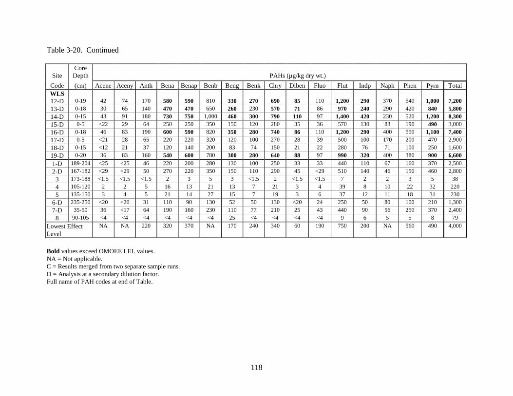
Table 3-20. Continued

118

CoreSite Depth PAHs (µg/kg dry wt.)

Code (cm) Acene Aceny Anth Bena Benap Benb Beng Benk Chry Diben Fluo Flut Indp Naph Phen Pyrn TotalWLS12-D 0-19 42 74 170 580 590 810 330 270 690 85 110 1,200 290 370 540 1,000 7,20013-D 0-18 30 65 140 470 470 650 260 230 570 71 86 970 240 290 420 840 5,80014-D 0-15 43 91 180 730 750 1,000 460 300 790 110 97 1,400 420 230 520 1,200 8,30015-D 0-5 <22 29 64 250 250 350 150 120 280 35 36 570 130 83 190 490 3,00016-D 0-18 46 83 190 600 590 820 350 280 740 86 110 1,200 290 400 550 1,100 7,40017-D 0-5 <21 28 65 220 220 320 120 100 270 28 39 500 100 170 200 470 2,90018-D 0-15 <12 21 37 120 140 200 83 74 150 21 22 280 76 71 100 250 1,60019-D 0-20 36 83 160 540 600 780 300 280 640 88 97 990 320 400 380 900 6,6001-D 189-204 <25 <25 46 220 200 280 130 100 250 33 33 440 110 67 160 370 2,5002-D 167-182 <29 <29 50 270 220 350 150 110 290 45 <29 510 140 46 150 460 2,800

3 173-188 <1.5 <1.5 <1.5 2 3 5 3 <1.5 2 <1.5 <1.5 7 2 2 3 5 384 105-120 2 2 5 16 13 21 13 7 21 3 4 39 8 10 22 32 2205 135-150 3 4 5 21 14 27 15 7 19 3 6 37 12 11 18 31 230

6-D 235-250 <20 <20 31 110 90 130 52 50 130 <20 24 250 50 80 100 210 1,3007-D 35-50 36 <17 64 190 160 230 110 77 210 25 43 440 90 56 250 370 2,400

8 90-105 <4 <4 <4 <4 <4 <4 25 <4 <4 <4 <4 9 6 5 5 8 79Lowest EffectLevel

NA NA 220 320 370 NA 170 240 340 60 190 750 200 NA 560 490 4,000

Bold values exceed OMOEE LEL values.NA = Not applicable.C = Results merged from two separate sample runs.D = Analysis at a secondary dilution factor.Full name of PAH codes at end of Table.

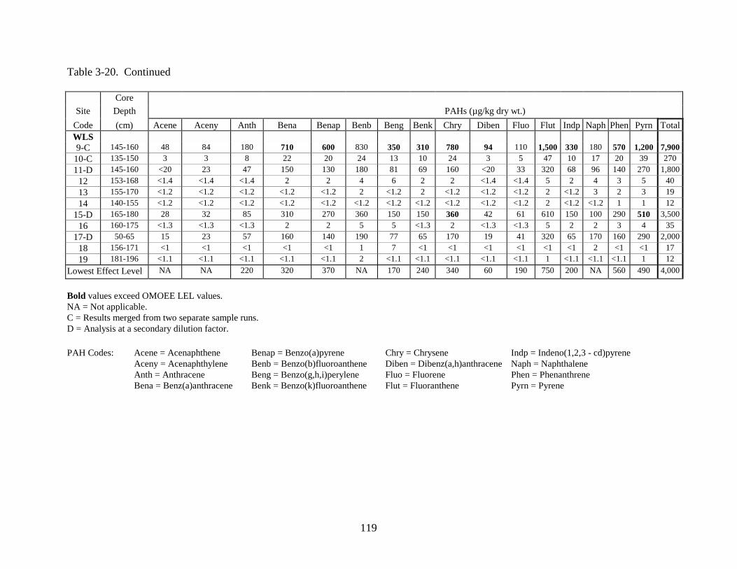
Table 3-20. Continued

119

CoreSite Depth PAHs (µg/kg dry wt.)

Code (cm) Acene Aceny Anth Bena Benap Benb Beng Benk Chry Diben Fluo Flut Indp Naph Phen Pyrn TotalWLS9-C 145-160 48 84 180 710 600 830 350 310 780 94 110 1,500 330 180 570 1,200 7,900

10-C 135-150 3 3 8 22 20 24 13 10 24 3 5 47 10 17 20 39 27011-D 145-160 <20 23 47 150 130 180 81 69 160 <20 33 320 68 96 140 270 1,800

12 153-168 <1.4 <1.4 <1.4 2 2 4 6 2 2 <1.4 <1.4 5 2 4 3 5 4013 155-170 <1.2 <1.2 <1.2 <1.2 <1.2 2 <1.2 2 <1.2 <1.2 <1.2 2 <1.2 3 2 3 1914 140-155 <1.2 <1.2 <1.2 <1.2 <1.2 <1.2 <1.2 <1.2 <1.2 <1.2 <1.2 2 <1.2 <1.2 1 1 12

15-D 165-180 28 32 85 310 270 360 150 150 360 42 61 610 150 100 290 510 3,50016 160-175 <1.3 <1.3 <1.3 2 2 5 5 <1.3 2 <1.3 <1.3 5 2 2 3 4 35

17-D 50-65 15 23 57 160 140 190 77 65 170 19 41 320 65 170 160 290 2,00018 156-171 <1 <1 <1 <1 <1 1 7 <1 <1 <1 <1 <1 <1 2 <1 <1 1719 181-196 <1.1 <1.1 <1.1 <1.1 <1.1 2 <1.1 <1.1 <1.1 <1.1 <1.1 1 <1.1 <1.1 <1.1 1 12

Lowest Effect Level NA NA 220 320 370 NA 170 240 340 60 190 750 200 NA 560 490 4,000

Bold values exceed OMOEE LEL values.NA = Not applicable.C = Results merged from two separate sample runs.D = Analysis at a secondary dilution factor.

PAH Codes: Acene = Acenaphthene Benap = Benzo(a)pyrene Chry = Chrysene Indp = Indeno(1,2,3 - cd)pyreneAceny = Acenaphthylene Benb = Benzo(b)fluoroanthene Diben = Dibenz(a,h)anthracene Naph = NaphthaleneAnth = Anthracene Beng = Benzo(g,h,i)perylene Fluo = Fluorene Phen = PhenanthreneBena = Benz(a)anthracene Benk = Benzo(k)fluoroanthene Flut = Fluoranthene Pyrn = Pyrene

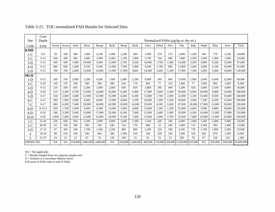
Table 3-21. TOC-normalized PAH Results for Selected Sites

120

CoreSite Depth Normalized PAHs (µg/kg oc dry wt.)

Code (cm) Acene Aceny Anth Bena Benap Benb Beng Benk Chry Diben Fluo Flut Indp Naph Phen Pyrn Total

KMB1-C 0-8 59 160 400 1,900 2,100 3,400 1,200 960 1,800 370 170 2,400 1,200 540 770 2,100 20,000

2-C 0-12 160 440 940 5,800 5,900 9,400 1,100 1,900 5,700 760 400 7,600 2,500 1,600 1,900 7,000 53,000

3-D 0-15 500 500 1,900 10,000 9,400 12,000 2,700 4,500 10,000 1,700 1,300 14,000 5,200 4,800 4,200 12,000 97,000

4-D 0-15 680 680 1,400 9,100 9,500 11,000 7,300 5,000 9,500 1,700 680 13,000 5,400 3,600 4,100 10,000 91,000

5-D 0-15 700 700 2,000 13,000 14,000 15,000 17,000 6400 14,000 2,400 1,500 17,000 7,500 3,200 5,400 14,000 130,000

MLH1-D 0-12 260 760 2,000 5,200 4,200 7,000 2,400 2,200 6,800 560 860 13,000 1,900 2,600 6,600 12,000 68,000

2-C 0-20 140 370 200 390 280 490 160 170 460 77 310 1,400 77 1,800 990 1,000 8,300

3-D 0-15 210 580 830 2,200 1,900 2,800 830 820 2,800 280 490 5,300 920 3,600 2,500 4,000 30,000

4-D 0-20 510 3,300 4,700 15,000 14,000 20,000 6,400 6,400 17,000 2,000 2,400 29,000 6,000 20,000 9,800 23,000 180,000

5-D 0-17 530 2,600 3,400 12,000 12,000 15,000 6,600 6,200 13,000 1,700 2,000 22,000 5,100 13,000 8,500 18,000 140,000

6-C 0-21 380 1,900 2,900 9,400 8,000 12,000 4,600 3,100 10,000 1,300 1,200 18,000 3,500 7,100 6,200 15,000 100,000

7-C 0-17 680 4,200 7,600 29,000 34,000 42,000 19,000 16,000 29,000 4,500 2,600 47,000 18,000 17,000 12,000 39,000 320,000

8-D 0-15.5 560 1,700 2,900 9,400 9,200 13,000 5,800 4,800 12,000 1,300 1,200 23,000 4,600 5,000 8,800 18,000 120,000

9-D 0-20 540 3,200 5,600 19,000 17,000 22,000 8,100 7,600 21,000 2,400 2,400 35,000 6,300 14,000 11,000 27,000 210,000

10-D 0-20 1,800 1,400 5,000 12,000 14,000 18,000 9,100 7,400 15,000 2,000 2,700 25,000 7,600 10,000 11,000 20,000 160,000

1-C 25-40 230 600 850 3,200 2,800 4,000 1,600 1,300 3,100 420 340 6,000 1,600 1,200 2,400 5,000 34,000

2-C 80-95 63 350 280 580 330 630 120 170 680 53 240 1,800 110 5,300 580 1,400 13,000

3-D 37-52 87 360 450 1,700 1,500 2,200 800 800 2,200 220 290 4,100 730 1,700 1,800 3,500 23,000

4 30-50 88 250 160 540 460 580 1,300 210 540 100 130 1,300 320 620 670 1,200 8,300

5 32-47 23 23 23 67 76 130 100 23 81 23 23 200 76 67 130 210 1,300OMOEE SEL NA NA 370,000 1,480,000 1,440,000 NA 320,000 1,340,000 460,000 130,000 160,000 1,020,000 320,000 NA 950,000 850,000 10,000,000

NA = Not applicableC = Results merged from two separate sample runs.D = Analysis at a secondary dilution factor.Full name of PAH codes at end of Table.

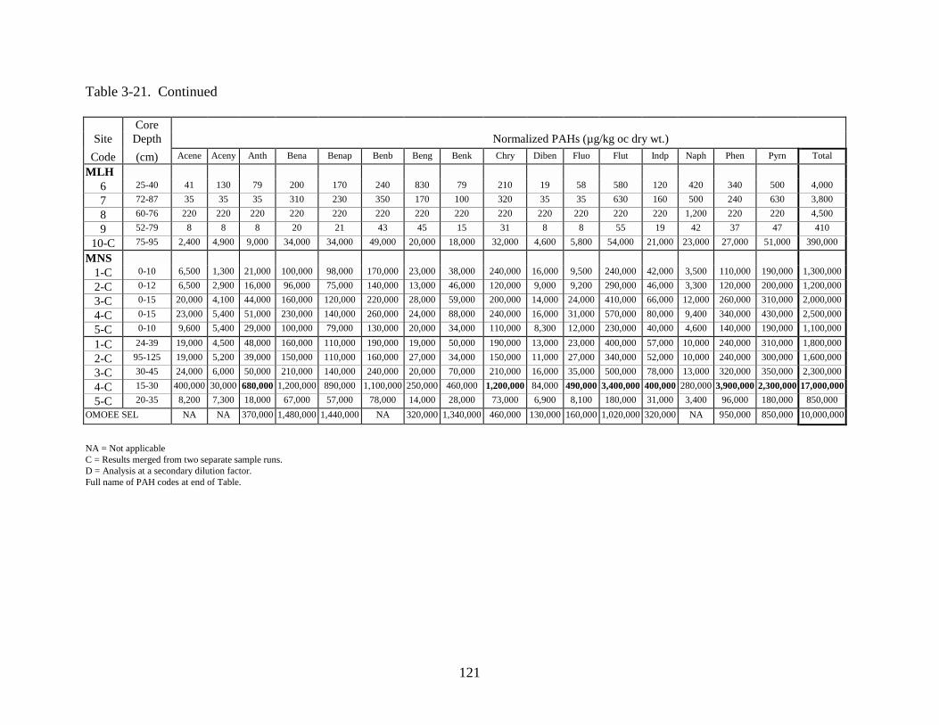
Table 3-21. Continued

121

CoreSite Depth Normalized PAHs (µg/kg oc dry wt.)

Code (cm) Acene Aceny Anth Bena Benap Benb Beng Benk Chry Diben Fluo Flut Indp Naph Phen Pyrn Total

MLH6 25-40 41 130 79 200 170 240 830 79 210 19 58 580 120 420 340 500 4,000

7 72-87 35 35 35 310 230 350 170 100 320 35 35 630 160 500 240 630 3,800

8 60-76 220 220 220 220 220 220 220 220 220 220 220 220 220 1,200 220 220 4,500

9 52-79 8 8 8 20 21 43 45 15 31 8 8 55 19 42 37 47 410

10-C 75-95 2,400 4,900 9,000 34,000 34,000 49,000 20,000 18,000 32,000 4,600 5,800 54,000 21,000 23,000 27,000 51,000 390,000

MNS1-C 0-10 6,500 1,300 21,000 100,000 98,000 170,000 23,000 38,000 240,000 16,000 9,500 240,000 42,000 3,500 110,000 190,000 1,300,000

2-C 0-12 6,500 2,900 16,000 96,000 75,000 140,000 13,000 46,000 120,000 9,000 9,200 290,000 46,000 3,300 120,000 200,000 1,200,000

3-C 0-15 20,000 4,100 44,000 160,000 120,000 220,000 28,000 59,000 200,000 14,000 24,000 410,000 66,000 12,000 260,000 310,000 2,000,000

4-C 0-15 23,000 5,400 51,000 230,000 140,000 260,000 24,000 88,000 240,000 16,000 31,000 570,000 80,000 9,400 340,000 430,000 2,500,000

5-C 0-10 9,600 5,400 29,000 100,000 79,000 130,000 20,000 34,000 110,000 8,300 12,000 230,000 40,000 4,600 140,000 190,000 1,100,000

1-C 24-39 19,000 4,500 48,000 160,000 110,000 190,000 19,000 50,000 190,000 13,000 23,000 400,000 57,000 10,000 240,000 310,000 1,800,000

2-C 95-125 19,000 5,200 39,000 150,000 110,000 160,000 27,000 34,000 150,000 11,000 27,000 340,000 52,000 10,000 240,000 300,000 1,600,000

3-C 30-45 24,000 6,000 50,000 210,000 140,000 240,000 20,000 70,000 210,000 16,000 35,000 500,000 78,000 13,000 320,000 350,000 2,300,000

4-C 15-30 400,000 30,000 680,000 1,200,000 890,000 1,100,000 250,000 460,000 1,200,000 84,000 490,000 3,400,000 400,000 280,000 3,900,000 2,300,000 17,000,000

5-C 20-35 8,200 7,300 18,000 67,000 57,000 78,000 14,000 28,000 73,000 6,900 8,100 180,000 31,000 3,400 96,000 180,000 850,000OMOEE SEL NA NA 370,000 1,480,000 1,440,000 NA 320,000 1,340,000 460,000 130,000 160,000 1,020,000 320,000 NA 950,000 850,000 10,000,000

NA = Not applicableC = Results merged from two separate sample runs.D = Analysis at a secondary dilution factor.Full name of PAH codes at end of Table.

Table 3-21. Continued

122

CoreSite Depth Normalized PAHs (µg/kg oc dry wt.)

Code (cm) Acene Aceny Anth Bena Benap Benb Beng Benk Chry Diben Fluo Flut Indp Naph Phen Pyrn Total

STP12-D 0-15 1,800 320 2,700 11,000 10,000 13,000 4,100 5,600 13,000 2,000 2,700 21,000 6,100 2,200 16,000 17,000 130,000

12-C 15-30 4,700 2,600 4,700 14,000 10,000 15,000 2,000 6,000 15,000 2,100 8,700 26,000 5,500 2,300 55,000 23,000 200,000

12-D 30-46 1,600 1,000 3,800 14,000 14,000 18,000 5,700 5,700 17,000 2,600 3,200 24,000 7,300 4,000 14,000 22,000 160,000

12-D 76-91 1,300 1,300 5,600 20,000 20,000 30,000 5,600 7,000 20,000 3,400 3,600 41,000 10,000 3,800 19,000 34,000 220,000

SUS1-D 0-15 1,700 850 3,600 13,000 13,000 19,000 8,700 6,400 16,000 2,600 2,300 28,000 7,900 2,600 16,000 23,000 160,000

2-C 0-15 3,100 1,300 6,800 24,000 25,000 34,000 15,000 11,000 27,000 4,600 4,600 60,000 14,000 4,800 28,000 48,000 310,000

3-C 0-15 35,000 1,800 57,000 73,000 67,000 84,000 24,000 33,000 69,000 11,000 53,000 180,000 31,000 11,000 200,000 150,000 1,100,000

4-C 0-15 5,300 2,300 10,000 32,000 37,000 49,000 23,000 19,000 40,000 6,300 7,400 81,000 20,000 5,600 51,000 70,000 460,000

5-C 0-15 4,800 1,300 11,000 32,000 34,000 43,000 20,000 13,000 34,000 6,100 6,100 74,000 18,000 4,800 43,000 61,000 410,000

6-C 0-15 10,000 1,400 38,000 95,000 110,000 120,000 50,000 39,000 100,000 15,000 10,000 240,000 45,000 3,300 130,000 260,000 1,300,000

7-D 0-5 2,100 780 5,600 16,000 16,000 21,000 9,600 7,000 18,000 2,900 3,400 32,000 8,100 3,300 23,000 28,000 200,000

1-C 30-45 2,400 870 3,300 6,700 6,400 9,300 3,200 2,700 9,300 870 3,500 17,000 2,900 1,900 17,000 14,000 100,000

2-C 30-45 2,000 320 2,800 8,900 10,000 13,000 3,700 4,400 12,000 1,200 2,400 20,000 3,800 2,300 15,000 20,000 120,000

3-C 30-45 2,200 1,800 5,600 14,000 15,000 21,000 6,700 6,900 17,000 2,000 3,600 33,000 6,700 2,800 25,000 27,000 190,000

4-C 30-45 4,600 4,900 10,000 32,000 35,000 42,000 16,000 14,000 32,000 4,200 5,800 70,000 15,000 4,400 37,000 63,000 400,000

5-D 24-38 3,500 1,100 7,800 22,000 24,000 35,000 12,000 12,000 26,000 3,100 6,100 54,000 12,000 5,800 44,000 46,000 310,000

6-D 30-45 12,000 3,000 21,000 50,000 43,000 64,000 27,000 27,000 54,000 3,000 18,000 130,000 22,000 29,000 140,000 110,000 750,000

7-D 30-45 4,400 2,100 7,100 17,000 18,000 23,000 8,600 8,600 17,000 2,200 4,900 41,000 7,900 4,300 31,000 37,000 240,000OMOEE SEL NA NA 370,000 1,480,000 1,440,000 NA 320,000 1,340,000 460,000 130,000 160,000 1,020,000 320,000 NA 950,000 850,000 10,000,000

NA = Not applicableC = Results merged from two separate sample runs.D = Analysis at a secondary dilution factor.Full name of PAH codes at end of Table.

Table 3-21. Continued

123

CoreSite Depth Normalized PAHs (µg/kg oc dry wt.)

Code (cm) Acene Aceny Anth Bena Benap Benb Beng Benk Chry Diben Fluo Flut Indp Naph Phen Pyrn Total

WLS1-C 0-15 3,000 3,000 9,000 48,000 45,000 76,000 29,000 25,000 59,000 9,000 3,800 100,000 30,000 2,200 32,000 83,000 550,000

2-C 0-15 2,300 23,000 7,000 37,000 34,000 52,000 22,000 16,000 40,000 6,500 3,100 70,000 22,000 2,500 26,000 56,000 420,000

3-C 0-17 2,200 2,500 7,100 30,000 27,000 45,000 18,000 13,000 31,000 5,500 3,200 55,000 18,000 3,200 22,000 45,000 320,000

4-C 0-20 1,900 2,900 6,300 33,000 31,000 50,000 20,000 16,000 37,000 6,300 2,800 63,000 21,000 2,500 20,000 53,000 370,000

5-D 0-18 960 1,800 3,500 18,000 16,000 26,000 10,000 8,200 18,000 3,300 1,600 31,000 11,000 3,500 8,600 26,000 190,000

6-D 0-15 1,200 2,100 4,600 24,000 23,000 38,000 15,000 10,000 25,000 4,600 2,000 43,000 16,000 3,800 13,000 38,000 260,000

7-C 0-15 860 1,500 2,800 12,000 14,000 19,000 10,000 7,700 15,000 2,000 1,400 25,000 8,000 2,700 9,100 23,000 150,000

8-C 0-15 1,600 3,100 5,800 24,000 22,000 36,000 13,000 11,000 27,000 4,400 3,100 42,000 14,000 6,900 15,000 38,000 270,000

9-C 0-20 1,100 2,000 3,900 19,000 19,000 29,000 12,000 9,200 20,000 3,700 1,900 34,000 12,000 3,900 10,000 29,000 210,000

10-C 0-15 1,000 2,000 3,300 14,000 16,000 22,000 10,000 8,800 17,000 2,500 1,800 27,000 8,200 4,400 8,800 26,000 170,000

11-C 0-20 1,000 2,200 3,600 14,000 17,000 25,000 11,000 8,300 19,000 2,000 1,900 28,000 9,200 6,100 10,000 26,000 190,000

12-D 0-19 860 1,500 3,500 12,000 12,000 16,000 6,700 5,500 14,000 1,700 2,200 24,000 5,900 7,600 11,000 20,000 150,000

13-D 0-18 640 1,400 3,000 10,000 10,000 14,000 5,500 4,900 12,000 1,500 1,800 21,000 5,100 6,200 8,900 18,000 120,000

14-D 0-15 770 1,600 3,200 13,000 13,000 18,000 8,200 5,400 14,000 2,000 1,700 25,000 7,500 4,100 9,300 21,000 150,000

15-D 0-5 420 1,100 2,500 9,600 9,600 13,000 5,800 4,600 11,000 1,300 1,400 22,000 5,000 3,200 7,300 19,000 120,000

16-D 0-18 980 1,800 4,000 13,000 12,000 17,000 7,400 6,000 16,000 1,800 2,300 26,000 6,200 8,500 12,000 23,000 160,000

17-D 0-5 380 1,000 2,300 7,800 7,800 11,000 4,300 3,600 9,600 1,000 1,400 18,000 3,600 6,100 7,100 17,000 100,000

18-D 0-15 220 780 1,400 4,400 5,200 7,400 3,100 2,700 5,600 780 820 10,000 2,800 2,600 3,700 9,200 59,000

19-D 0-20 820 1,900 3,600 12,000 14,000 18,000 6,800 6,400 14,000 2,000 2,200 22,000 7,300 9,100 8,600 20,000 150,000

OMOEE SEL NA NA 370,000 1,480,000 1,440,000 NA 320,000 1,340,000 460,000 130,000 160,000 1,020,000 320,000 NA 950,000 850,000 10,000,000

NA = Not applicableC = Results merged from two separate sample runs.D = Analysis at a secondary dilution factor.Full name of PAH codes at end of Table.

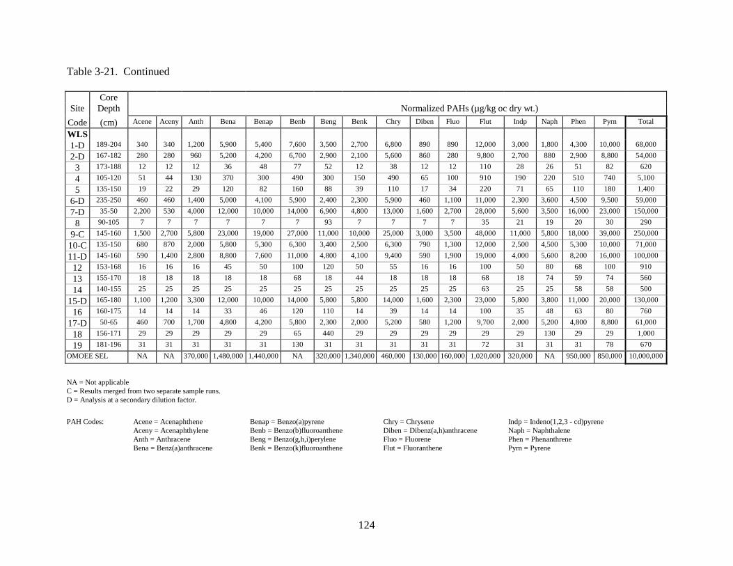
Table 3-21. Continued

124

CoreSite Depth Normalized PAHs (µg/kg oc dry wt.)

Code (cm) Acene Aceny Anth Bena Benap Benb Beng Benk Chry Diben Fluo Flut Indp Naph Phen Pyrn Total

WLS1-D 189-204 340 340 1,200 5,900 5,400 7,600 3,500 2,700 6,800 890 890 12,000 3,000 1,800 4,300 10,000 68,000

2-D 167-182 280 280 960 5,200 4,200 6,700 2,900 2,100 5,600 860 280 9,800 2,700 880 2,900 8,800 54,000

3 173-188 12 12 12 36 48 77 52 12 38 12 12 110 28 26 51 82 620

4 105-120 51 44 130 370 300 490 300 150 490 65 100 910 190 220 510 740 5,100

5 135-150 19 22 29 120 82 160 88 39 110 17 34 220 71 65 110 180 1,400

6-D 235-250 460 460 1,400 5,000 4,100 5,900 2,400 2,300 5,900 460 1,100 11,000 2,300 3,600 4,500 9,500 59,000

7-D 35-50 2,200 530 4,000 12,000 10,000 14,000 6,900 4,800 13,000 1,600 2,700 28,000 5,600 3,500 16,000 23,000 150,000

8 90-105 7 7 7 7 7 7 93 7 7 7 7 35 21 19 20 30 290

9-C 145-160 1,500 2,700 5,800 23,000 19,000 27,000 11,000 10,000 25,000 3,000 3,500 48,000 11,000 5,800 18,000 39,000 250,000

10-C 135-150 680 870 2,000 5,800 5,300 6,300 3,400 2,500 6,300 790 1,300 12,000 2,500 4,500 5,300 10,000 71,000

11-D 145-160 590 1,400 2,800 8,800 7,600 11,000 4,800 4,100 9,400 590 1,900 19,000 4,000 5,600 8,200 16,000 100,000

12 153-168 16 16 16 45 50 100 120 50 55 16 16 100 50 80 68 100 910

13 155-170 18 18 18 18 18 68 18 44 18 18 18 68 18 74 59 74 560

14 140-155 25 25 25 25 25 25 25 25 25 25 25 63 25 25 58 58 500

15-D 165-180 1,100 1,200 3,300 12,000 10,000 14,000 5,800 5,800 14,000 1,600 2,300 23,000 5,800 3,800 11,000 20,000 130,000

16 160-175 14 14 14 33 46 120 110 14 39 14 14 100 35 48 63 80 760

17-D 50-65 460 700 1,700 4,800 4,200 5,800 2,300 2,000 5,200 580 1,200 9,700 2,000 5,200 4,800 8,800 61,000

18 156-171 29 29 29 29 29 65 440 29 29 29 29 29 29 130 29 29 1,000

19 181-196 31 31 31 31 31 130 31 31 31 31 31 72 31 31 31 78 670OMOEE SEL NA NA 370,000 1,480,000 1,440,000 NA 320,000 1,340,000 460,000 130,000 160,000 1,020,000 320,000 NA 950,000 850,000 10,000,000

NA = Not applicableC = Results merged from two separate sample runs.D = Analysis at a secondary dilution factor.

PAH Codes: Acene = Acenaphthene Benap = Benzo(a)pyrene Chry = Chrysene Indp = Indeno(1,2,3 - cd)pyreneAceny = Acenaphthylene Benb = Benzo(b)fluoroanthene Diben = Dibenz(a,h)anthracene Naph = NaphthaleneAnth = Anthracene Beng = Benzo(g,h,i)perylene Fluo = Fluorene Phen = PhenanthreneBena = Benz(a)anthracene Benk = Benzo(k)fluoroanthene Flut = Fluoranthene Pyrn = Pyrene

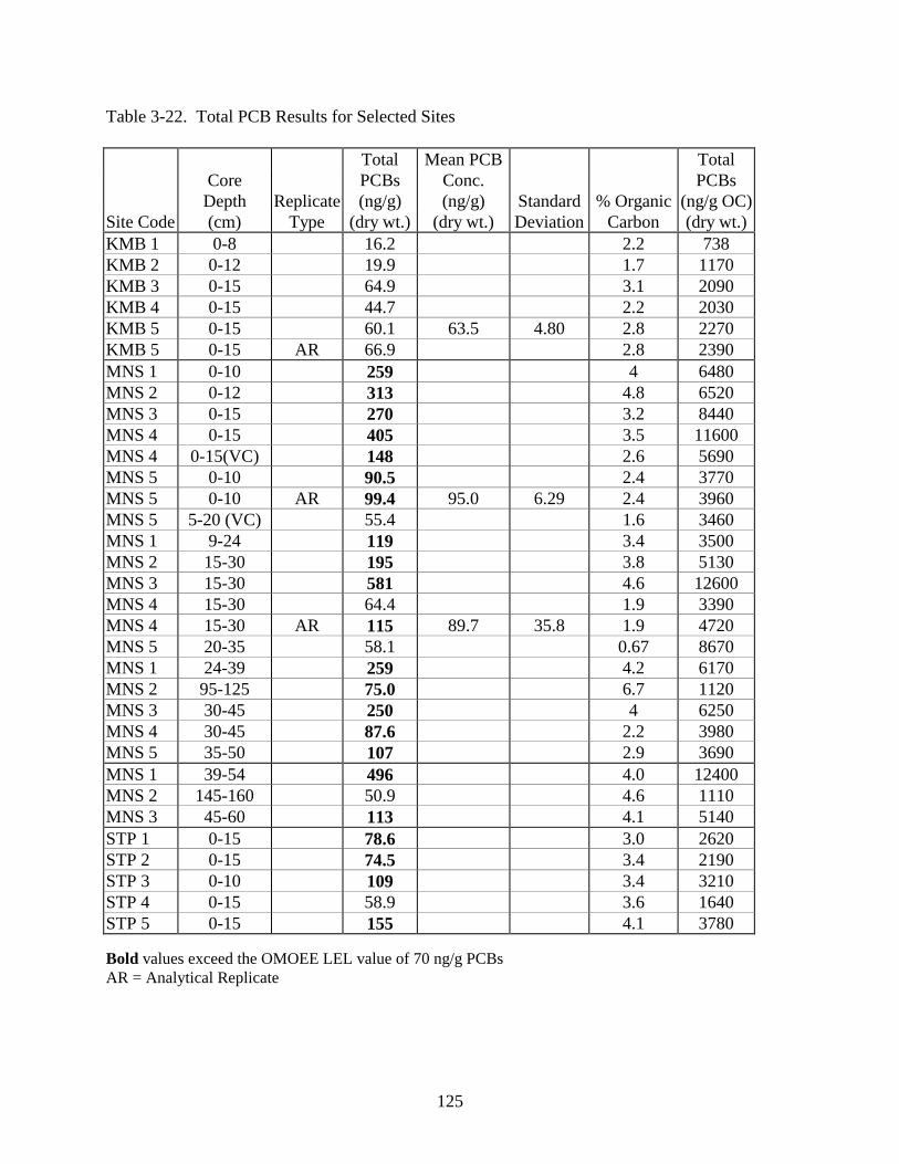
Table 3-22. Total PCB Results for Selected Sites

125

Total Mean PCB TotalCore PCBs Conc. PCBsDepth Replicate (ng/g) (ng/g) Standard % Organic (ng/g OC)

Site Code (cm) Type (dry wt.) (dry wt.) Deviation Carbon (dry wt.)KMB 1 0-8 16.2 2.2 738KMB 2 0-12 19.9 1.7 1170KMB 3 0-15 64.9 3.1 2090KMB 4 0-15 44.7 2.2 2030KMB 5 0-15 60.1 63.5 4.80 2.8 2270KMB 5 0-15 AR 66.9 2.8 2390MNS 1 0-10 259 4 6480MNS 2 0-12 313 4.8 6520MNS 3 0-15 270 3.2 8440MNS 4 0-15 405 3.5 11600MNS 4 0-15(VC) 148 2.6 5690MNS 5 0-10 90.5 2.4 3770MNS 5 0-10 AR 99.4 95.0 6.29 2.4 3960MNS 5 5-20 (VC) 55.4 1.6 3460MNS 1 9-24 119 3.4 3500MNS 2 15-30 195 3.8 5130MNS 3 15-30 581 4.6 12600MNS 4 15-30 64.4 1.9 3390MNS 4 15-30 AR 115 89.7 35.8 1.9 4720MNS 5 20-35 58.1 0.67 8670MNS 1 24-39 259 4.2 6170MNS 2 95-125 75.0 6.7 1120MNS 3 30-45 250 4 6250MNS 4 30-45 87.6 2.2 3980MNS 5 35-50 107 2.9 3690MNS 1 39-54 496 4.0 12400MNS 2 145-160 50.9 4.6 1110MNS 3 45-60 113 4.1 5140STP 1 0-15 78.6 3.0 2620STP 2 0-15 74.5 3.4 2190STP 3 0-10 109 3.4 3210STP 4 0-15 58.9 3.6 1640STP 5 0-15 155 4.1 3780

Bold values exceed the OMOEE LEL value of 70 ng/g PCBsAR = Analytical Replicate

Table 3-22. Continued

126

Total Mean PCB TotalCore PCBs Conc. PCBsDepth Replicate (ng/g) (ng/g) Standard % Organic (ng/g OC)

Site Code (cm) Type (dry wt.) (dry wt.) Deviation Carbon (dry wt.)STP 6 0-15 69.6 3.4 2050STP 6 0-15 AR 64.7 67.2 3.46 3.4 1980STP 7 0-15 109 3.2 3410STP 8 0-15 140 5 2800STP 10 0-10 121 3.4 3560STP 12 0-10 116 4.1 2830STP 1 15-30 139 4 3480STP 2 10-25 213 4.5 4730STP 3 15-30 35.6 3.9 913STP 4 15-30 48.1 3.4 1420STP 6 7-23 62.6 3.2 1960STP 7 5-23 99.7 3.2 3120STP 7 5-23 AR 101 100.4 0.919 3.2 3140STP 8 15-30 88.1 5 1760STP 8 15-30 AR 86.3 87.2 1.27 5 1740STP 12 15-30 549 4.7 11700STP 1 30-45 145 2.3 6300STP 3 30-45 21.1 1.8 1170STP 4 30-45 69.2 4.6 1500STP 6 23-38 81.5 3.6 2260STP 12 30-46 353 3.7 9540STP 12 76-91 30.4 6.4 475SUS 1 0-15 220 4.7 4681SUS 1 0-15 AR 190 205 21.2 4.7 4040SUS 2 0-15 121 3.5 3460SUS 3 0-15 326 4.9 6650SUS 4 0-15 132 4.3 3070SUS 5 0-15 134 2.3 5830SUS 6 0-15 95.0 1.9 5000SUS 7 0-5 102 2.7 3780

Bold values exceed the OMOEE LEL value of 70 ng/g PCBsAR = Analytical Replicate

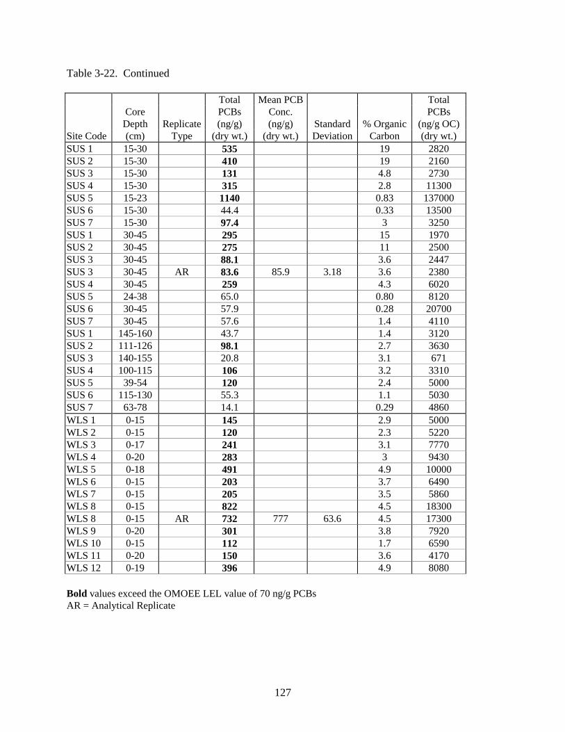
Table 3-22. Continued

127

Total Mean PCB TotalCore PCBs Conc. PCBsDepth Replicate (ng/g) (ng/g) Standard % Organic (ng/g OC)

Site Code (cm) Type (dry wt.) (dry wt.) Deviation Carbon (dry wt.)SUS 1 15-30 535 19 2820SUS 2 15-30 410 19 2160SUS 3 15-30 131 4.8 2730SUS 4 15-30 315 2.8 11300SUS 5 15-23 1140 0.83 137000SUS 6 15-30 44.4 0.33 13500SUS 7 15-30 97.4 3 3250SUS 1 30-45 295 15 1970SUS 2 30-45 275 11 2500SUS 3 30-45 88.1 3.6 2447SUS 3 30-45 AR 83.6 85.9 3.18 3.6 2380SUS 4 30-45 259 4.3 6020SUS 5 24-38 65.0 0.80 8120SUS 6 30-45 57.9 0.28 20700SUS 7 30-45 57.6 1.4 4110SUS 1 145-160 43.7 1.4 3120SUS 2 111-126 98.1 2.7 3630SUS 3 140-155 20.8 3.1 671SUS 4 100-115 106 3.2 3310SUS 5 39-54 120 2.4 5000SUS 6 115-130 55.3 1.1 5030SUS 7 63-78 14.1 0.29 4860WLS 1 0-15 145 2.9 5000WLS 2 0-15 120 2.3 5220WLS 3 0-17 241 3.1 7770WLS 4 0-20 283 3 9430WLS 5 0-18 491 4.9 10000WLS 6 0-15 203 3.7 6490WLS 7 0-15 205 3.5 5860WLS 8 0-15 822 4.5 18300WLS 8 0-15 AR 732 777 63.6 4.5 17300WLS 9 0-20 301 3.8 7920WLS 10 0-15 112 1.7 6590WLS 11 0-20 150 3.6 4170WLS 12 0-19 396 4.9 8080

Bold values exceed the OMOEE LEL value of 70 ng/g PCBsAR = Analytical Replicate

Table 3-22. Continued

128

Total Mean PCB TotalCore PCBs Conc. PCBsDepth Replicate (ng/g) (ng/g) Standard % Organic (ng/g OC)

Site Code (cm) Type (dry wt.) (dry wt.) Deviation Carbon (dry wt.)WLS 13 0-18 491 4.7 10400WLS 14 0-15 346 5.6 6180WLS 15 0-5 366 2.6 14100WLS 16 0-18 424 4.7 9020WLS 17 0-5 215 2.8 7680WLS 18 0-15 94.3 2.7 3490WLS 18 0-15 AR 93.6 94.0 0.495 2.7 3480WLS 19 0-20 271 4.4 6160WLS 1 15-30 590 3.3 1790WLS 2 15-30 13.8 1 1380WLS 3 15-30 117 3.5 3340WLS 4 15-30 40.5 1.1 3680WLS 5 15-30 422 8.7 4850WLS 5 15-30 AR 460 441 26.9 8.7 5070WLS 6 15-30 571 2.8 20400WLS 7 5-20 679 3.7 18400WLS 8 15-30 4.40 3.9 113WLS 9 15-30 No Data AvailableWLS 10 15-30 21.3 2.6 819WLS 11 15-30 535 4.2 12700WLS 12 15-30 77.2 3.5 2210WLS 13 15-30 876 4.3 20400WLS 14 15-30 14.6 2.3 635WLS 15 15-30 10.8 1.8 600WLS 16 15-30 463 3.7 12500WLS 17 15-30 44.0 3 1470WLS 17 15-30 AR 42.9 43.5 0.778 3 1450WLS 18 15-30 14.1 1.9 742WLS 19 15-30 18.2 2.7 674WLS 1 30-45 1220 3.3 37000WLS 2 30-45 15.3 1 1530WLS 2 30-45 AR 23.8 19.6 6.01 1 1960WLS 3 30-45 435 4.5 9670WLS 4 30-45 39.0 0.76 5130

Bold values exceed the OMOEE LEL value of 70 ng/g PCBsAR = Analytical Replicate

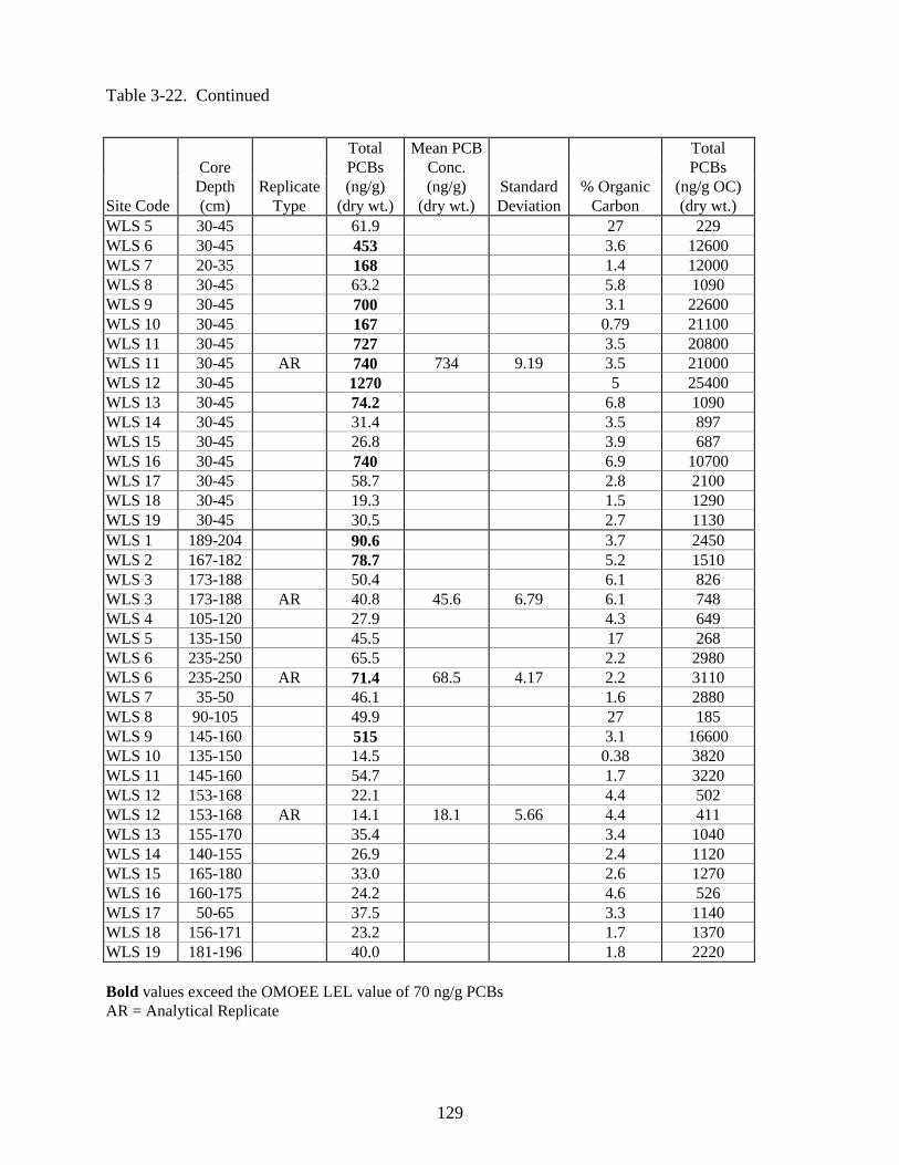
Table 3-22. Continued

129

Total Mean PCB TotalCore PCBs Conc. PCBsDepth Replicate (ng/g) (ng/g) Standard % Organic (ng/g OC)

Site Code (cm) Type (dry wt.) (dry wt.) Deviation Carbon (dry wt.)WLS 5 30-45 61.9 27 229WLS 6 30-45 453 3.6 12600WLS 7 20-35 168 1.4 12000WLS 8 30-45 63.2 5.8 1090WLS 9 30-45 700 3.1 22600WLS 10 30-45 167 0.79 21100WLS 11 30-45 727 3.5 20800WLS 11 30-45 AR 740 734 9.19 3.5 21000WLS 12 30-45 1270 5 25400WLS 13 30-45 74.2 6.8 1090WLS 14 30-45 31.4 3.5 897WLS 15 30-45 26.8 3.9 687WLS 16 30-45 740 6.9 10700WLS 17 30-45 58.7 2.8 2100WLS 18 30-45 19.3 1.5 1290WLS 19 30-45 30.5 2.7 1130WLS 1 189-204 90.6 3.7 2450WLS 2 167-182 78.7 5.2 1510WLS 3 173-188 50.4 6.1 826WLS 3 173-188 AR 40.8 45.6 6.79 6.1 748WLS 4 105-120 27.9 4.3 649WLS 5 135-150 45.5 17 268WLS 6 235-250 65.5 2.2 2980WLS 6 235-250 AR 71.4 68.5 4.17 2.2 3110WLS 7 35-50 46.1 1.6 2880WLS 8 90-105 49.9 27 185WLS 9 145-160 515 3.1 16600WLS 10 135-150 14.5 0.38 3820WLS 11 145-160 54.7 1.7 3220WLS 12 153-168 22.1 4.4 502WLS 12 153-168 AR 14.1 18.1 5.66 4.4 411WLS 13 155-170 35.4 3.4 1040WLS 14 140-155 26.9 2.4 1120WLS 15 165-180 33.0 2.6 1270WLS 16 160-175 24.2 4.6 526WLS 17 50-65 37.5 3.3 1140WLS 18 156-171 23.2 1.7 1370WLS 19 181-196 40.0 1.8 2220

Bold values exceed the OMOEE LEL value of 70 ng/g PCBsAR = Analytical Replicate

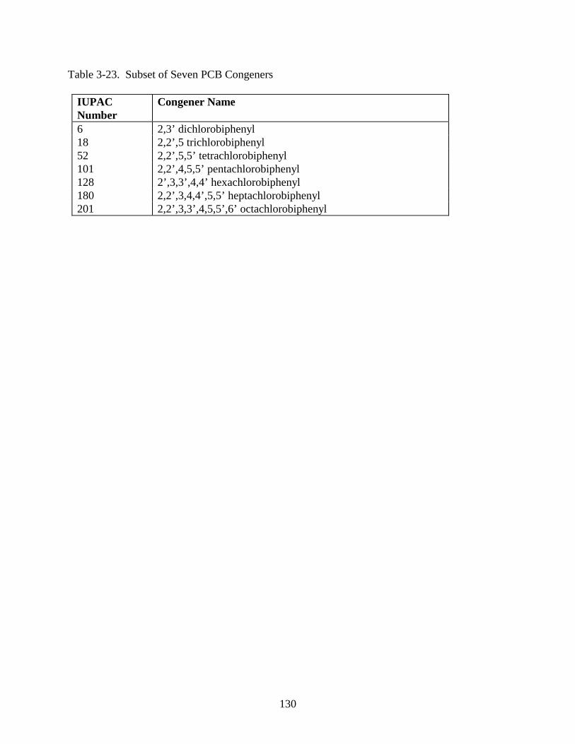
Table 3-23. Subset of Seven PCB Congeners

130

IUPACNumber

Congener Name

6 2,3’ dichlorobiphenyl18 2,2’,5 trichlorobiphenyl52 2,2’,5,5’ tetrachlorobiphenyl101 2,2’,4,5,5’ pentachlorobiphenyl128 2’,3,3’,4,4’ hexachlorobiphenyl180 2,2’,3,4,4’,5,5’ heptachlorobiphenyl201 2,2’,3,3’,4,5,5’,6’ octachlorobiphenyl

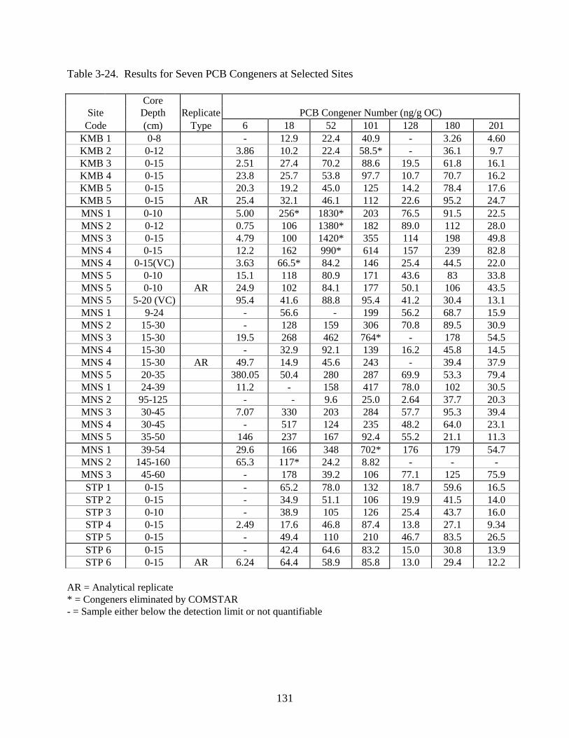
Table 3-24. Results for Seven PCB Congeners at Selected Sites

131

CoreSite Depth Replicate PCB Congener Number (ng/g OC)

Code (cm) Type 6 18 52 101 128 180 201KMB 1 0-8 - 12.9 22.4 40.9 - 3.26 4.60KMB 2 0-12 3.86 10.2 22.4 58.5* - 36.1 9.7KMB 3 0-15 2.51 27.4 70.2 88.6 19.5 61.8 16.1KMB 4 0-15 23.8 25.7 53.8 97.7 10.7 70.7 16.2KMB 5 0-15 20.3 19.2 45.0 125 14.2 78.4 17.6KMB 5 0-15 AR 25.4 32.1 46.1 112 22.6 95.2 24.7MNS 1 0-10 5.00 256* 1830* 203 76.5 91.5 22.5MNS 2 0-12 0.75 106 1380* 182 89.0 112 28.0MNS 3 0-15 4.79 100 1420* 355 114 198 49.8MNS 4 0-15 12.2 162 990* 614 157 239 82.8MNS 4 0-15(VC) 3.63 66.5* 84.2 146 25.4 44.5 22.0MNS 5 0-10 15.1 118 80.9 171 43.6 83 33.8MNS 5 0-10 AR 24.9 102 84.1 177 50.1 106 43.5MNS 5 5-20 (VC) 95.4 41.6 88.8 95.4 41.2 30.4 13.1MNS 1 9-24 - 56.6 - 199 56.2 68.7 15.9MNS 2 15-30 - 128 159 306 70.8 89.5 30.9MNS 3 15-30 19.5 268 462 764* - 178 54.5MNS 4 15-30 - 32.9 92.1 139 16.2 45.8 14.5MNS 4 15-30 AR 49.7 14.9 45.6 243 - 39.4 37.9MNS 5 20-35 380.05 50.4 280 287 69.9 53.3 79.4MNS 1 24-39 11.2 - 158 417 78.0 102 30.5MNS 2 95-125 - - 9.6 25.0 2.64 37.7 20.3MNS 3 30-45 7.07 330 203 284 57.7 95.3 39.4MNS 4 30-45 - 517 124 235 48.2 64.0 23.1MNS 5 35-50 146 237 167 92.4 55.2 21.1 11.3MNS 1 39-54 29.6 166 348 702* 176 179 54.7MNS 2 145-160 65.3 117* 24.2 8.82 - - -MNS 3 45-60 - 178 39.2 106 77.1 125 75.9STP 1 0-15 - 65.2 78.0 132 18.7 59.6 16.5STP 2 0-15 - 34.9 51.1 106 19.9 41.5 14.0STP 3 0-10 - 38.9 105 126 25.4 43.7 16.0STP 4 0-15 2.49 17.6 46.8 87.4 13.8 27.1 9.34STP 5 0-15 - 49.4 110 210 46.7 83.5 26.5STP 6 0-15 - 42.4 64.6 83.2 15.0 30.8 13.9STP 6 0-15 AR 6.24 64.4 58.9 85.8 13.0 29.4 12.2

AR = Analytical replicate* = Congeners eliminated by COMSTAR- = Sample either below the detection limit or not quantifiable

Table 3-24. Continued

132

CoreSite Depth Replicate PCB Congener Number (ng/g OC)

Code (cm) Type 6 18 52 101 128 180 201STP 7 0-15 - 65.1 93.6 169 30.0 57.9 19.6STP 8 0-15 - 40.7 97.4 120 36.1 57.3 24.2STP 10 0-10 - 128 111 170 39.1 73.4 24.6STP 12 0-10 - 36.6 85.7 165 40.7 65.3 19.1STP 1 15-30 - 64.7 129 187 37.1 70.5 20.3STP 2 10-25 - 51.9 167 254 60.3 97.4 32.8STP 3 15-30 18.8 80.4 33.7 8.94 3.35 5.68 7.60STP 4 15-30 8.50 51.4 54.4 64.1 14.7 19.2 8.12STP 6 7-23 - 56.3 79.1 88.4 20.5 30.4 16.1STP 7 5-23 - 59.8 91.2 149 36.9 55.4 27.1STP 7 5-23 AR - 76.1 90.9 151 37.5 54.2 24.3STP 8 15-30 - 35.1 66.7 59.5 16.1 26.1 15.2STP 8 15-30 AR - 45.3 67.0 57.6 16.5 25.6 15.6STP 12 15-30 29.3 221 401 680 118 250 62.4STP 1 30-45 8.83 105 231 375 76.7 106 34.5STP 3 30-45 7.97 140 62.0 25.3 5.42 2.67 7.68STP 4 30-45 - 46.6 43.8 65.8 12.8 22.2 11.3STP 6 23-38 - 62.3 67.0 109 20.9 37.5 15.4STP 12 30-46 9.63 138 299 519 99.4 161 111STP 12 76-91 1.96 51.9 * 7.6 10.4 2.88 3.08 3.06SUS 1 0-15 - 346 * 153 222 50.3 108 29.2SUS 1 0-15 AR - 229 * 140 179 35.1 110 28.6SUS 2 0-15 - 177 113 175 46.6 106 27.2SUS 3 0-15 - 61.4 295 299 75.6 135 5.10SUS 4 0-15 5.61 80.5 118 154 45.5 42.8 22.0SUS 5 0-15 2.85 184 201 306 60.2 104 32.2SUS 6 0-15 4.71 168 184 255 42.0 97.3 33.0SUS 7 0-5 0.74 135 156 177 19.5 65.9 22.7SUS 1 15-30 0.39 40.0 85.2 131 * 32.6 61.6 11.8SUS 2 15-30 1.00 26.4 60.7 92.4 28.0 42.8 9.88SUS 3 15-30 - 73.7 - 93.2 48.8 56.0 15.3SUS 4 15-30 5.75 110 378 501 129 179 40.4SUS 5 15-23 5.86 88.9 6250 9378 2680 1510 148SUS 6 15-30 - 96.2 690 802 79.0 150 47.4SUS 7 15-30 - 54.7 76.3 121 30.9 60.1 20.0SUS 1 30-45 - 46.3 45.3 97.7 25.4 53.1 14.1SUS 2 30-45 - 95.1 * 87.9 134 43.8 60.9 0.273SUS 3 30-45 - 64.2 * 2.7 4.93 2.42 5.56 1.59

AR = Analytical replicate* = Congeners eliminated by COMSTAR- = Sample either below the detection limit or not quantifiable

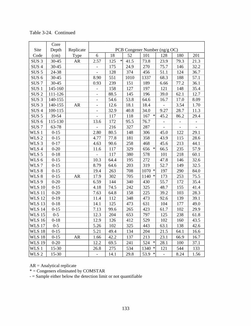
Table 3-24. Continued

133

CoreSite Depth Replicate PCB Congener Number (ng/g OC)

Code (cm) Type 6 18 52 101 128 180 201SUS 3 30-45 AR 2.57 125 * 41.5 73.8 23.9 79.3 21.3SUS 4 30-45 - 175 24.9 270 75.7 146 32.2SUS 5 24-38 - 128 374 456 51.1 124 36.7SUS 6 30-45 8.90 551 1010 1337 68.3 188 57.1SUS 7 30-45 0.93 239 151 189 6.66 77.2 36.1SUS 1 145-160 - 158 127 197 121 148 35.4SUS 2 111-126 - 88.5 145 196 39.0 62.1 12.7SUS 3 140-155 - 54.6 53.8 64.6 16.7 17.0 8.09SUS 3 140-155 AR - 12.6 18.1 18.4 - 3.54 1.70SUS 4 100-115 - 32.9 40.8 34.0 9.27 28.7 11.3SUS 5 39-54 - 117 118 167 * 45.2 86.2 29.4SUS 6 115-130 13.6 172 95.5 76.7 - - -SUS 7 63-78 - 216 327 287 - - -

WLS 1 0-15 2.80 80.5 148 306 45.0 122 29.1WLS 2 0-15 4.77 77.8 181 358 43.9 115 28.6WLS 3 0-17 4.63 90.6 258 468 45.6 213 44.1WLS 4 0-20 11.6 117 329 656 * 66.5 235 57.9WLS 5 0-18 - 117 380 578 101 218 60.1WLS 6 0-15 10.3 64.4 195 272 47.8 146 32.6WLS 7 0-15 8.79 64.6 203 319 52.7 149 32.5WLS 8 0-15 19.4 263 708 1070 * 197 290 84.0WLS 8 0-15 AR 17.9 302 705 1140 * 173 253 75.5WLS 9 0-20 6.59 144 340 430 55.7 172 35.4WLS 10 0-15 4.18 74.5 242 325 48.7 155 41.4WLS 11 0-20 7.63 64.8 158 225 39.2 103 28.3WLS 12 0-19 11.4 112 348 473 92.6 139 39.1WLS 13 0-18 14.1 125 473 631 104 177 49.0WLS 14 0-15 7.13 99.6 265 423 61.7 102 29.9WLS 15 0-5 12.3 204 653 797 125 238 61.8WLS 16 0-18 12.9 126 412 529 102 160 43.5WLS 17 0-5 5.26 102 325 443 63.1 138 42.6WLS 18 0-15 5.21 49.4 134 204 21.5 64.1 16.6WLS 18 0-15 AR 1.66 42.2 137 213 23.1 66.9 16.7WLS 19 0-20 12.2 69.5 241 524 * 28.1 100 37.1WLS 1 15-30 26.8 275 534 1340 * 121 544 133WLS 2 15-30 - 14.1 29.8 53.9 * - 8.24 1.56

AR = Analytical replicate* = Congeners eliminated by COMSTAR- = Sample either below the detection limit or not quantifiable

Table 3-24. Continued

134

CoreSite Depth Replicate PCB Congener Number (ng/g OC)

Code (cm) Type 6 18 52 101 128 180 201WLS 3 15-30 10.6 33.2 77.5 * 237 * 9.52 82.7 24.7WLS 4 15-30 - 14.6 200 244 - 86.0 21.2WLS 5 15-30 9.85 20.6 132 351 37.5 92.8 32.8WLS 5 15-30 AR 6.86 94.8 156 231 85.4 96.8 37.6WLS 6 15-30 56.1 292 860 1470 * 135 435 111WLS 7 5-20 39.4 283 764 1200 55.3 416 110WLS 8 15-30 - 2.80 4.6 7.36 * - - -WLS 8 15-30 AR - 3.89 6.5 * 6.40 * - - -WLS 9 15-30 No Data AvailableWLS 10 15-30 3.23 7.10 22.4 * 55.9 * 4.36 14.3 3.64WLS 11 15-30 18.2 207 503 630 106 322 82.7WLS 12 15-30 - 37.2 80.6 125 * 6.55 43.1 13.2WLS 13 15-30 113 158 816 1390 239 339 132WLS 14 15-30 3.06 22.0 27.8 42.2 * - - -WLS 15 15-30 3.16 25.5 24.9 40.2 * - 0.73 0.57WLS 16 15-30 31.1 150 571 909 146 229 76.9WLS 17 15-30 - 26.8 33.7 85.9 * - 28.8 7.08WLS 17 15-30 AR - 23.8 34.4 83.8 * - 27.8 6.75WLS 18 15-30 2.14 27.2 26.5 53.5 * - 3.69 -WLS 19 15-30 2.85 4.40 23.4 39.1 * - 5.34 3.32WLS 1 30-45 78.5 748 886 1720 * 283 1280 288WLS 2 30-45 5.00 124 74.0 85.0 - - 2.00WLS 2 30-45 AR 7.00 529 63.0 79.0 - 6.00 4.00WLS 3 30-45 8.40 458 396 592 97.9 182 75.2WLS 4 30-45 - 141 205 286 18.2 73.4 30.7WLS 5 30-45 2.09 78.59 * 4.9 3.35 0.63 1.30 0.54WLS 6 30-45 22.7 291 509 601 65.3 282 81.8WLS 7 20-35 29.3 317 443 693 * 70.9 270 84.2WLS 8 30-45 11.2 468 * 25.8 19.3 6.84 - 0.386WLS 9 30-45 15.2 493 1000.0 1230 139 400 107WLS 10 30-45 - 5840 184.8 211 43.9 53.6 11.2WLS 11 30-45 26.2 769 1110 733 67.9 240 73.1

AR = Analytical replicate* = Congeners eliminated by COMSTAR- = Sample either below the detection limit or not quantifiable

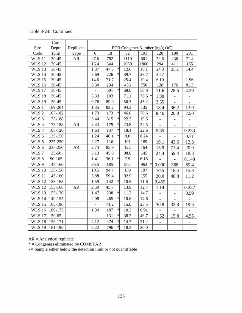
Table 3-24. Continued

135

CoreSite Depth Replicate PCB Congener Number (ng/g OC)

Code (cm) Type 6 18 52 101 128 180 201WLS 11 30-45 AR 27.6 782 1110 801 72.6 236 71.4WLS 12 30-45 16.4 344 1050 1860 294 411 155WLS 13 30-45 1.37 47.5 * 12.6 16.1 24.3 25.2 14.4WLS 14 30-45 5.69 226 * 39.7 28.7 3.47 - -WLS 15 30-45 14.6 71.7 25.4 19.4 6.10 - 1.96WLS 16 30-45 3.30 234 453 750 128 176 81.3WLS 17 30-45 - 501 * 68.8 50.8 11.6 28.5 4.29WLS 18 30-45 5.33 103 71.1 76.5 * 1.39 - -WLS 19 30-45 0.76 89.9 50.3 45.2 2.55 - -WLS 1 189-204 1.35 82.2 94.3 135 18.4 36.2 13.0WLS 2 167-182 1.73 173 * 46.0 70.6 8.46 20.0 7.50WLS 3 173-188 3.44 315 * 22.3 19.5 - - -WLS 3 173-188 AR 4.43 179 * 23.8 22.5 - - -WLS 4 105-120 1.63 137 * 18.4 22.6 5.35 - 0.233WLS 5 135-150 1.24 40.1 * 8.0 8.24 - - 0.71WLS 6 235-250 2.27 116 101 169 19.1 43.6 12.3WLS 6 235-250 AR 2.73 85.9 122 164 15.9 71.4 20.0WLS 7 35-50 3.13 45.0 98.8 145 24.4 59.4 18.8WLS 8 90-105 1.41 36.1 * 7.9 6.15 - - 0.148WLS 9 145-160 35.5 185 502 962 * 0.000 368 69.4WLS 10 135-150 10.5 94.7 139 197 10.5 18.4 15.8WLS 11 145-160 5.88 59.4 92.9 155 20.0 48.8 11.2WLS 12 153-168 1.59 142 * 10.5 11.6 0.455 - -WLS 12 153-168 AR 2.50 45.7 13.9 12.7 1.14 - 0.227WLS 13 155-170 1.47 238 * 11.2 14.7 - - 0.59WLS 14 140-155 2.08 465 * 10.8 14.6 - - -WLS 15 165-180 - 71.2 15.0 23.5 30.8 33.8 19.6WLS 16 160-175 1.30 187 * 10.2 8.91 - - -WLS 17 50-65 - 131 * 38.2 46.7 1.52 15.8 4.55WLS 18 156-171 4.12 474 * 14.7 21.2 - - -WLS 19 181-196 2.22 796 * 18.3 20.0 - - -

AR = Analytical replicate* = Congeners eliminated by COMSTAR- = Sample either below the detection limit or not quantifiable

Table 3-25. Mean Survival (%) of H. azteca and C. tentans Exposed to Test Sediments

136

Mean Survival (%) Mean Survival (%)Sample # H. azteca C. tentans Sample # H. azteca C. tentansDMIR 01 70* 72* WLS 03 72 80DMIR 02 95 88 WLS 04 98 78DMIR 03 82 72 WLS 06 90 80DMIR 04 98 75 WLS 08 90 80ERP 01 67 78 WLS 12 96 58ERP 02 58* 90 WLS 13 96 45ERP 03 80 60 WLS 14 96 50HOB 07 96 60 WLS 16 93 42HOB 08 100 28HOB 10 95 80HOB 11 68 70HOB 12 55* 70HOB 13 52* 72HOB 14 85 80HOB 15 78 80KMB 04 78 48KMB 05 80 65MLH 01 75 75MLH 02 80 70MLH 03 90 70MLH 04 65* 72MLH 05 82 82MLH 06 92 92MNS 01 89 28MNS 03 100 30STP 01 79 58STP 03 80 62STP 04 96 65STP 06 50 68STP 07 68 68SUS 01 85 72SUS 03 92 55*SUS 05 96 40SUS 07 45 0WLS 01 85 68*WLS 02 90 90

*Mean survival significantly less than control survival at p = 0.05.Shaded values indicate unacceptable contol survival.

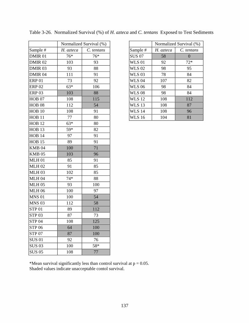
Table 3-26. Normalized Survival (%) of H. azteca and C. tentans Exposed to Test Sediments

137

Normalized Survival (%) Normalized Survival (%)Sample # H. azteca C. tentans Sample # H. azteca C. tentansDMIR 01 76* 76* SUS 07 58 0DMIR 02 103 93 WLS 01 92 72*DMIR 03 93 88 WLS 02 98 95DMIR 04 111 91 WLS 03 78 84ERP 01 73 92 WLS 04 107 82ERP 02 63* 106 WLS 06 98 84ERP 03 103 88 WLS 08 98 84HOB 07 108 115 WLS 12 108 112HOB 08 112 54 WLS 13 108 87HOB 10 108 91 WLS 14 108 96HOB 11 77 80 WLS 16 104 81HOB 12 63* 80HOB 13 59* 82HOB 14 97 91HOB 15 89 91KMB 04 100 71KMB 05 103 96MLH 01 85 91MLH 02 91 85MLH 03 102 85MLH 04 74* 88MLH 05 93 100MLH 06 100 97MNS 01 100 54MNS 03 112 58STP 01 89 112STP 03 87 73STP 04 108 125STP 06 64 100STP 07 87 100SUS 01 92 76SUS 03 100 58*SUS 05 108 77

*Mean survival significantly less than control survival at p = 0.05.Shaded values indicate unacceptable contol survival.

138

Table 3-27. Mean Total Abundance (individuals/m2) and Taxa Richness Values for theBenthological Community Survey

Site# ofReplicates

MeanTotalAbundance SD*

MeanTaxaRichness SD*

DMIR 1 1 215 149 3 2

DMIR 2 1 1,120 637 6 2

DMIR 3 1 804 813 7 6

DMIR 4 1 2,986 1,318 18 5

ERP 1 3 7,640 1,998 11 2

ERP 2 3 6,311 2,233 13 3

ERP 3 3 14,283 5,887 17 5

ERP 5 3 4,900 1,007 7 3

HOB 1 3 3,238 1,556 6 2

HOB 2 3 7,308 4,245 11 4

HOB 3 3 11,751 12,697 10 6

HOB 4 3 7,100 4,758 9 2

HOB 5 3 9,135 3,102 10 2

HOB 6 3 3,737 1,318 8 3

HOB 7 3 15,114 3,462 15 1

HOB 8 2 249 249 1 1

HOB 9 2 249 249 1 1

HOB 10 3 2,740 1,556 6 3

HOB 11 3 2,865 778 6 1

HOB 12 3 3,073 1,416 7 3

HOB 13 3 6,975 2,215 10 0

HOB 14 3 8,221 4,244 9 4

HOB 15 3 4,484 1,515 10 3

KMB 1 3 2,325 1,767 4 1

KMB 2 3 1,578 943 4 2

*SD = standard deviation

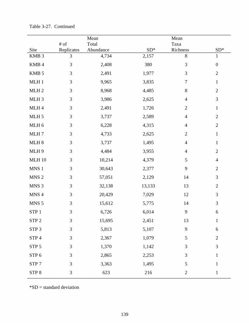
139

Table 3-27. Continued

Site# ofReplicates

MeanTotalAbundance SD*

MeanTaxaRichness SD*

KMB 3 3 4,734 2,157 8 1

KMB 4 3 2,408 380 3 0

KMB 5 3 2,491 1,977 3 2

MLH 1 3 9,965 3,835 7 1

MLH 2 3 8,968 4,485 8 2

MLH 3 3 3,986 2,625 4 3

MLH 4 3 2,491 1,726 2 1

MLH 5 3 3,737 2,589 4 2

MLH 6 3 6,228 4,315 4 2

MLH 7 3 4,733 2,625 2 1

MLH 8 3 3,737 1,495 4 1

MLH 9 3 4,484 3,955 4 2

MLH 10 3 10,214 4,379 5 4

MNS 1 3 30,643 2,377 9 2

MNS 2 3 57,051 2,129 14 3

MNS 3 3 32,138 13,133 13 2

MNS 4 3 20,429 7,029 12 3

MNS 5 3 15,612 5,775 14 3

STP 1 3 6,726 6,014 9 6

STP 2 3 15,695 2,451 13 1

STP 3 3 5,813 5,107 9 6

STP 4 3 2,367 1,079 5 2

STP 5 3 1,370 1,142 3 3

STP 6 3 2,865 2,253 3 1

STP 7 3 3,363 1,495 5 1

STP 8 3 623 216 2 1

*SD = standard deviation

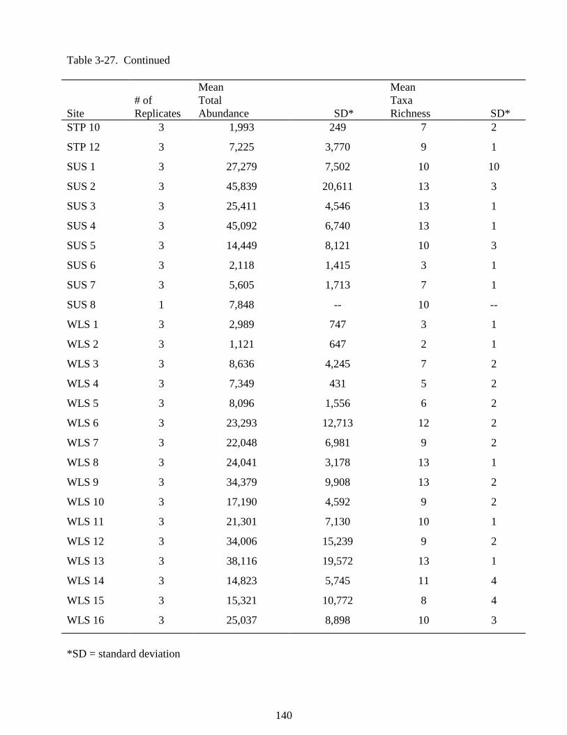
140

Table 3-27. Continued

Site# ofReplicates

MeanTotalAbundance SD*

MeanTaxaRichness SD*

STP 10 3 1,993 249 7 2

STP 12 3 7,225 3,770 9 1

SUS 1 3 27,279 7,502 10 10

SUS 2 3 45,839 20,611 13 3

SUS 3 3 25,411 4,546 13 1

SUS 4 3 45,092 6,740 13 1

SUS 5 3 14,449 8,121 10 3

SUS 6 3 2,118 1,415 3 1

SUS 7 3 5,605 1,713 7 1

SUS 8 1 7,848 -- 10 --

WLS 1 3 2,989 747 3 1

WLS 2 3 1,121 647 2 1

WLS 3 3 8,636 4,245 7 2

WLS 4 3 7,349 431 5 2

WLS 5 3 8,096 1,556 6 2

WLS 6 3 23,293 12,713 12 2

WLS 7 3 22,048 6,981 9 2

WLS 8 3 24,041 3,178 13 1

WLS 9 3 34,379 9,908 13 2

WLS 10 3 17,190 4,592 9 2

WLS 11 3 21,301 7,130 10 1

WLS 12 3 34,006 15,239 9 2

WLS 13 3 38,116 19,572 13 1

WLS 14 3 14,823 5,745 11 4

WLS 15 3 15,321 10,772 8 4

WLS 16 3 25,037 8,898 10 3

*SD = standard deviation

141

Table 3-27. Continued

Site# ofReplicates

MeanTotalAbundance SD*

MeanTaxaRichness SD*

WLS 17 3 36,041 18,657 15 2

WLS 18 3 11,460 2,403 6 2

WLS 19 3 14,699 4,427 9 1

*SD = standard deviation

142

Table 3-28. Mean Densities (number/m2), with Sample Standard Deviations in Parentheses, andPercent Composition of each Macroinvertebrate Group for the DMIR Sites (n=3)

Taxon DMIR 1 DMIR 2 DMIR 3 DMIR 4

Tubificidae 158 (90) 919 (585) 632 (151) 1765 (807)73% 82% 79% 59%

Naididae - - - Less 1%

Polychaeta - - 14 (25) 100 (25)2% 3%

Nematoda 14 (25) - - 2%7%

Turbellaria - 3% - -

Bivalvia 14 (25) 158 (90) 100 (25) 273 (108)7% 14% 12% 9%

Gastropoda - - - -

Hydrachnida - - - -

Chironomidae 14 (25) 14 (25) 43 (75) 646 (258)7% 1% 5% 22%

Chaoboridae 14 (25) - - 76 (66)7% 2%

Ephemeroptera - - 2% -

Trichoptera - - - 1%

miscellaneous - - - 1%

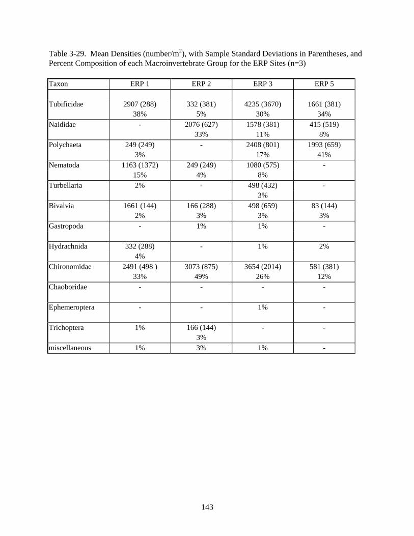
143

Table 3-29. Mean Densities (number/m2), with Sample Standard Deviations in Parentheses, andPercent Composition of each Macroinvertebrate Group for the ERP Sites (n=3)

Taxon ERP 1 ERP 2 ERP 3 ERP 5

Tubificidae 2907 (288) 332 (381) 4235 (3670) 1661 (381)38% 5% 30% 34%

Naididae - 2076 (627) 1578 (381) 415 (519)33% 11% 8%

Polychaeta 249 (249) - 2408 (801) 1993 (659)3% 17% 41%

Nematoda 1163 (1372) 249 (249) 1080 (575) -15% 4% 8%

Turbellaria 2% - 498 (432) -3%

Bivalvia 1661 (144) 166 (288) 498 (659) 83 (144)2% 3% 3% 3%

Gastropoda - 1% 1% -

Hydrachnida 332 (288) - 1% 2%4%

Chironomidae 2491 (498 ) 3073 (875) 3654 (2014) 581 (381)33% 49% 26% 12%

Chaoboridae - - - -

Ephemeroptera - - 1% -

Trichoptera 1% 166 (144) - -3%

miscellaneous 1% 3% 1% -

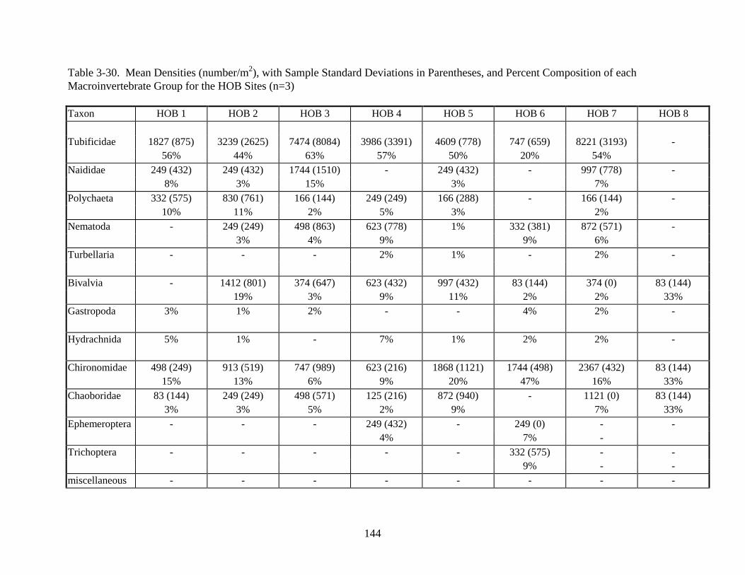
144

Table 3-30. Mean Densities (number/m2), with Sample Standard Deviations in Parentheses, and Percent Composition of eachMacroinvertebrate Group for the HOB Sites (n=3)

Taxon HOB 1 HOB 2 HOB 3 HOB 4 HOB 5 HOB 6 HOB 7 HOB 8

Tubificidae 1827 (875) 3239 (2625) 7474 (8084) 3986 (3391) 4609 (778) 747 (659) 8221 (3193) -56% 44% 63% 57% 50% 20% 54%

Naididae 249 (432) 249 (432) 1744 (1510) - 249 (432) - 997 (778) -8% 3% 15% 3% 7%

Polychaeta 332 (575) 830 (761) 166 (144) 249 (249) 166 (288) - 166 (144) -10% 11% 2% 5% 3% 2%

Nematoda - 249 (249) 498 (863) 623 (778) 1% 332 (381) 872 (571) -3% 4% 9% 9% 6%

Turbellaria - - - 2% 1% - 2% -

Bivalvia - 1412 (801) 374 (647) 623 (432) 997 (432) 83 (144) 374 (0) 83 (144)19% 3% 9% 11% 2% 2% 33%

Gastropoda 3% 1% 2% - - 4% 2% -

Hydrachnida 5% 1% - 7% 1% 2% 2% -

Chironomidae 498 (249) 913 (519) 747 (989) 623 (216) 1868 (1121) 1744 (498) 2367 (432) 83 (144)15% 13% 6% 9% 20% 47% 16% 33%

Chaoboridae 83 (144) 249 (249) 498 (571) 125 (216) 872 (940) - 1121 (0) 83 (144)3% 3% 5% 2% 9% 7% 33%

Ephemeroptera - - - 249 (432) - 249 (0) - -4% 7% -

Trichoptera - - - - - 332 (575) - -9% - -

miscellaneous - - - - - - - -

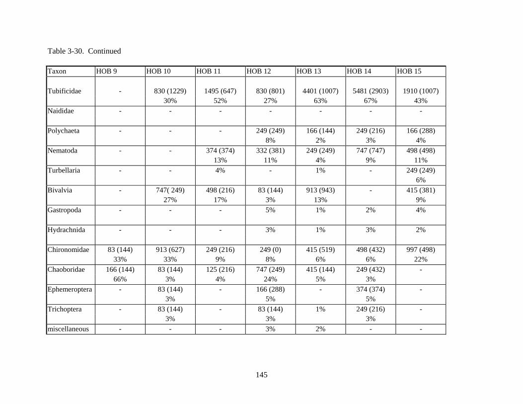
145

Table 3-30. Continued

Taxon HOB 9 HOB 10 HOB 11 HOB 12 HOB 13 HOB 14 HOB 15

Tubificidae - 830 (1229) 1495 (647) 830 (801) 4401 (1007) 5481 (2903) 1910 (1007)30% 52% 27% 63% 67% 43%

Naididae - - - - - - -

Polychaeta - - - 249 (249) 166 (144) 249 (216) 166 (288)8% 2% 3% 4%

Nematoda - - 374 (374) 332 (381) 249 (249) 747 (747) 498 (498)13% 11% 4% 9% 11%

Turbellaria - - 4% - 1% - 249 (249)6%

Bivalvia - 747( 249) 498 (216) 83 (144) 913 (943) - 415 (381)27% 17% 3% 13% 9%

Gastropoda - - - 5% 1% 2% 4%

Hydrachnida - - - 3% 1% 3% 2%

Chironomidae 83 (144) 913 (627) 249 (216) 249 (0) 415 (519) 498 (432) 997 (498)33% 33% 9% 8% 6% 6% 22%

Chaoboridae 166 (144) 83 (144) 125 (216) 747 (249) 415 (144) 249 (432) -66% 3% 4% 24% 5% 3%

Ephemeroptera - 83 (144) - 166 (288) - 374 (374) -3% 5% 5%

Trichoptera - 83 (144) - 83 (144) 1% 249 (216) -3% 3% 3%

miscellaneous - - - 3% 2% - -

146

Table 3-31. Mean Densities (number/m2), with Sample Standard Deviations in Parentheses, andPercent Composition of each Macroinvertebrate Group for the KMB Sites (n=3)

Taxon KMB 1 KMB 2 KMB 3 KMB 4 KMB 5

Tubificidae 498 (432) 166 (288 ) 1495 (898) 664 (381) 581 (144)21% 11% 32% 28% 23%

Naididae 581 (1007) - - - -25%

Polychaeta 581 (381) 166 (288) 1246 (863) - -25% 11% 26%

Nematoda 166 (288) 249 (249) - - -7% 16%

Turbellaria - - - - -

Bivalvia - 415 (381) 249 (249) 83 (144) -26% 5% 3%

Gastropoda 3% - 2% - -

Hydrachnida - - 249 (249) - -5%

Chironomidae 249 (432) 332 (144) 1163 (144) 83 (144) -11% 21% 25% 3%

Chaoboridae - 249 (249) 249 (249) 1578 (627) 1827 (1696)16% 5% 66% 73%

Ephemeroptera 83 (144) - - - -4%

Trichoptera 83 (144) - - - -4%

miscellaneous - - - - 3%

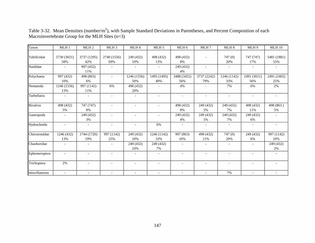
147

Table 3-32. Mean Densities (number/m2), with Sample Standard Deviations in Parentheses, and Percent Composition of eachMacroinvertebrate Group for the MLH Sites (n=3)

Taxon MLH 1 MLH 2 MLH 3 MLH 4 MLH 5 MLH 6 MLH 7 MLH 8 MLH 9 MLH 10

Tubificidae 5730 (3021) 3737 (1295) 2740 (1556) 249 (432) 498 (432) 498 (432) - 747 (0) 747 (747) 5481 (1881)58% 42% 69% 10% 13% 8% 20% 17% 55%

Naididae - 997 (432) - - - 249 (432) - - - -11% 4%

Polychaeta 997 (432) 498 (863) - 1246 (1556) 1495 (1495) 3488 (3452) 3737 (2242) 1246 (1142) 2491 (3021) 2491 (2402)10% 6% 50% 40% 56% 79% 33% 56% 25%

Nematoda 1246 (1556) 997 (1142) 6% 498 (432) - 4% - 7% 6% 2%13% 11% 20%

Turbellaria - - - - - - - - - -

Bivalvia 498 (432) 747 (747) - - - 498 (432) 249 (432) 249 (432) 498 (432) 498 (863 )5% 8% 8% 5% 7% 11% 5%

Gastropoda - 249 (432) - - - 249 (432) 249 (432) 249 (432) 249 (432) -3% 4% 5% 7% 6%

Hydrachnida - - - - 6% - - - - -

Chironomidae 1246 (432) 1744 (1726) 997 (1142) 249 (432) 1246 (1142) 997 (863) 498 (432) 747 (0) 249 (432) 997 (1142)13% 19% 25% 10% 33% 16% 11% 20% 6% 10%

Chaoboridae - - - 249 (432) 249 (432) - - - - 249 (432)10% 7% 2%

Ephemeroptera - - - - - - - - - -

Trichoptera 2% - - - - - - - - -

miscellaneous - - - - - - - 7% - -

148

Table 3-33. Mean Densities (number/m2), with Sample Standard Deviations in Parentheses, andPercent Composition of each Macroinvertebrate Group for the MNS Sites (n=3)

Taxon MNS 1 MNS 2 MNS 3 MNS 4 MNS 5

Tubificidae 27072 (2355) 50656 (2920) 25245 (10240) 13287 (6602) 9218 (3915)88% 89% 79% 65% 59%

Naididae 664 (288) 2491 (659) 3322 (2972) 830 (144) 830 (575 )2% 4% 10% 4% 5%

Polychaeta - Less 1% 1% 1993 (249) 249 (432)10% 2%

Nematoda Less 1% Less 1% 1744 (249) 1661 (144) 581 (144)5% 8% 4%

Turbellaria 913 (144) 1% 1% 1% 498 (659)3% 3%

Bivalvia 1744 (498 ) 2907 (761) 1163 (381) 1910 (575) 2823 (943)6% 5% 4% 9% 18%

Gastropoda 1% Less 1% Less 1% - 2%

Hydrachnida - - - 1% 2%

Chironomidae - 83 (144) 83 (144) 83 (144) 166 (288)Less 1% Less 1% Less 1% 1%

Chaoboridae - - - - -

Ephemeroptera - - - - -

Trichoptera - - - 1% 415 (144)3%

miscellaneous - - - Less 1% 2%

149

Table 3-34. Mean Densities (number/m2), with Sample Standard Deviations in Parentheses, and Percent Composition of eachMacroinvertebrate Group for the STP Sites (n=3)

Taxon STP 1 STP 2 STP 3 STP 4 STP 5 STP 6 STP 7 STP 8 STP 10 STP 12

Tubificidae 3737 (2616) 8470 (2755) 1204 (730) 1370 (718) 498 (432) 1744 (1312) 1495 (989) 374 (0) 830 (144) 3571 (1935)56% 54% 21% 58% 36% 61% 44% 60% 41% 49%

Naididae 997 (1415) 1121 (374) 2408 (2800) 125 (216) - - - - 83 (144) 332 (381)15% 7% 41% 5% 4% 5%

Polychaeta 374 (374) 1993 (216) - 125 (216) - 374 (374) 374 (374) - - 249 (0)6% 13% 5% 13% 11% 3%

Nematoda 4% 2% - - 125 (216) - - - - -9%

Turbellaria 4% - 1080 (1123) - 125 (216) - - - 4% -19% 9%

Bivalvia 374 (647) 498 (571) 332 (381) 374 (0) 125 (216) - 249 (216) - 166 (144) 2076 (1254)6% 3% 6% 16% 9% 7% 8% 28%

Gastropoda - 1% 1% 125 (216) 125 (216) - - - 4% -5% 9%

Hydrachnida 2% - 1% 125 (216) - 4% 4% - 4% -5%

Chironomidae 498 (432) 3114 (940) 540 (190) 125 (216) 249 (432) 623 (778) 1121 (374 ) 249 (216) 581 (144) 997 (898)7% 20% 9% 5% 18% 22% 33% 40% 29% 14%

Chaoboridae 2% - - - - - - - 4% -

Ephemeroptera - 1% - - 125 (216) - - - - -9%

Trichoptera - - - - - - - - - -

miscellaneous - - 1% - - - - - - -

150

Table 3-35. Mean Densities (number/m2), with Sample Standard Deviations in Parentheses, and Percent Composition of eachMacroinvertebrate Group for the SUS Sites (n=3 for SUS 1-7; n=1 for SUS 8)

Taxon SUS 1 SUS 2 SUS 3 SUS 4 SUS 5 SUS 6 SUS 7 SUS 8

Tubificidae 21549 (4819) 30892 (13161) 15820 (3668) 38490 (5505) 10463 (6921) - 623 (778) 74779% 67% 62% 85% 72% 11% 10%

Naididae 3114 (2830) 8595 (5389) 2118 (1201) 1370 (432) 747 (374) 1246 (1201) 1495 (1295) 373711% 19% 8% 3% 5% 59% 27% 48%

Polychaeta - - 1% - 2% - 2% -

Nematoda Less 1% 1% 1121 (374) 2% 374 (374) - - -4% 3%

Turbellaria 1% 1% 1% 1619 (1201) 747 (647) - - -4% 5%

Bivalvia 1495 (747) 3737 (1629) 3986 (1142) 1619 (778) 1% - 125 (216) 3745% 8% 16% 4% 2% 5%

Gastropoda - Less 1% 1% 1% - 6% - -

Hydrachnida Less 1% 1% - - 1% - - 5%

Chironomidae 498 (571) 1495 (747) 1619 (1312) 872 (778) 1370 (532) 623 (432) 2990 (747) 26162% 3% 6% 2% 9% 29% 53% 33%

Other Diptera - - - - - - 249 (216) -4%

Trichoptera - - - Less 1% 249 (432) 125 (216) - -2% 6%

151

Table 3-36. Mean Densities (number/m2) with Sample Standard Deviations in Parentheses, and Percent Composition of eachMacroinvertebrate Group for the WLS Sites (n=3)

Taxon WLS 1 WLS 2 WLS 3 WLS 4 WLS 5 WLS 6 WLS 7 WLS 8 WLS 9 WLS 10

Tubificidae 1246 (863) 872 (571) 3107 (2488) 4360 (1881) 5232 (374) 16442 (12028) 12083 (5046) 11584 (989) 24290 (12028) 6477 (571)42% 78% 59% 59% 65% 71% 55% 48% 71% 38%

Naididae 249 (432) - 374 (374) 125 (216) - 125 (216) - 1246 (571) 374 (647) 249 (432)8% 4% 2% 1% 5% 1% 1%

Polychaeta 498 (432) - 1246 (1556) 774 (774) 872 (216) 997 (571) 2865 (2625) 5854 (2544) 623 (216) 7847 (2966)17% 14% 10% 11% 4% 13% 24% 2% 46%

Nematoda - - 3% 2% 2% - 1% 3% Less 1% -

Turbellaria - - - - - 1% - - - -

Bivalvia 747 (747) 125 (216) 1370 (778) 1495 (374) 1370 (778) 3363 (1121) 5730 (571 ) 3488 (2058 ) 6602 (1415) 1619 (432)25% 11% 16% 20% 17% 14% 26% 15% 19% 9%

Gastropoda - - - - - - 1% - - -

Hydrachnida - - - - 3% - - - - -

Chironomidae - 125 (216) 291 (259) 498 (571) 125 (216) 1246 (1079) 623 (571) 997 (216) 1619 (216) 872 (432)11% 3% 7% 2% 5% 3% 4% 5% 5%

Chaoboridae - - - - - 997 (778) 374 (374) 1% 2% 1%4% 2%

Ephemeroptera - - - - - - - - - -

Trichoptera 249 (432) - - - 125 (216) - - 1% - -8% 2%

miscellaneous - - - - - - - - - -

152

Table 3-36. Continued

Taxon WLS 11 WLS 12 WLS 13 WLS 14 WLS 15 WLS 16 WLS 17 WLS 18 WLS 19

Tubificidae 14325 (7770) 23667 (8703 ) 29522 (17777) 5730 (3668) 4484 (2616) 17813 (4520) 14699 (4850) 3239 (1312) 5730 (1201)67% 70% 77% 39% 29% 71% 41% 28% 39%

Naididae 747 (0) 9218 (6646) 5605 (0) 872 (571) 125 (216) 4609 (3925) 1744 (1515) - -4% 27% 15% 6% 1% 18% 5%

Polychaeta - 249 (432) 1121 (1347) 6104 (1726) 8719 (7788) 997 (1079) 17522 (13831) 6104 (2158) 4609 (2830)1% 3% 41% 57% 4% 49% 53% 31%

Nematoda 1% - - 2% 2% Less 1% Less 1% 1121 (747) 1121 (747)10% 8%

Turbellaria - - - 1% - - - - -

Bivalvia 3861 (2544) - 747 (747) 747 (374) 747 (989) 498 (863) 581 (519) 623 (571) 2242 (0)18% 2% 5% 5% 2% 2% 5% 15%

Gastropoda - - - 1% 2% - Less 1% 2% -

Hydrachnida - - - - - - - - -

Chironomidae 374 (374) 872 (432) 1121 (374) 747 (747) 747 (374) 997 (940) 913 (381) 125 (216) 872 (571)1% 3% 3% 5% 5% 4% 3% 1% 6%

Chaoboridae 1868 (374) - - 1% - - - - -9%

Ephemeroptera - - - - - - Less 1% - -

Trichoptera - - - - - - Less 1% - -

miscellaneous - - - - - - - - -

153

Table 3-37. Number of Chironomid Larvae with Menta Deformities

Site Genus # Larvae with Deformities

DMIR 4 Procladius 1 of 21 larvae (4.8%)SUS 2 Procladius 1 of 12 larvae (8.3%)WLS 4 Procladius 1 of 4 larvae (25%)WLS 7 Chironomus 1 of 2 larvae (50%)WLS 13 Procladius 1 of 6 larvae (16.7%)WLS 19 Procladius 1 of 6 larvae (16.7%)

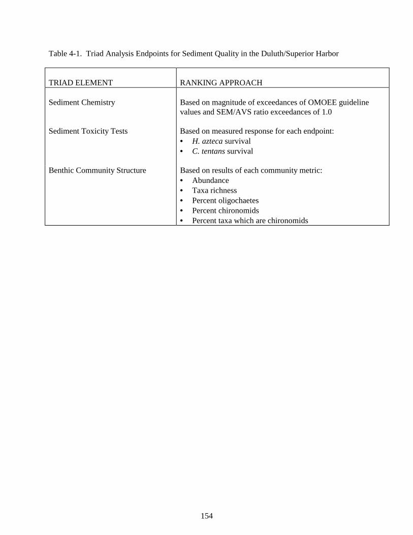
154

Table 4-1. Triad Analysis Endpoints for Sediment Quality in the Duluth/Superior Harbor

TRIAD ELEMENT RANKING APPROACH

Sediment Chemistry Based on magnitude of exceedances of OMOEE guidelinevalues and SEM/AVS ratio exceedances of 1.0

Sediment Toxicity Tests Based on measured response for each endpoint:• H. azteca survival• C. tentans survival

Benthic Community Structure Based on results of each community metric:• Abundance• Taxa richness• Percent oligochaetes• Percent chironomids• Percent taxa which are chironomids

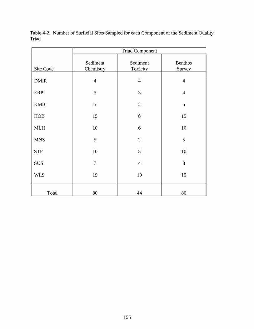
155

Table 4-2. Number of Surficial Sites Sampled for each Component of the Sediment QualityTriad

Triad Component

Site CodeSedimentChemistry

SedimentToxicity

BenthosSurvey

DMIR

ERP

KMB

HOB

MLH

MNS

STP

SUS

WLS

4

5

5

15

10

5

10

7

19

4

3

2

8

6

2

5

4

10

4

4

5

15

10

5

10

8

19

Total 80 44 80

APPENDIX A

SEDIMENT CHEMISTRY DATA

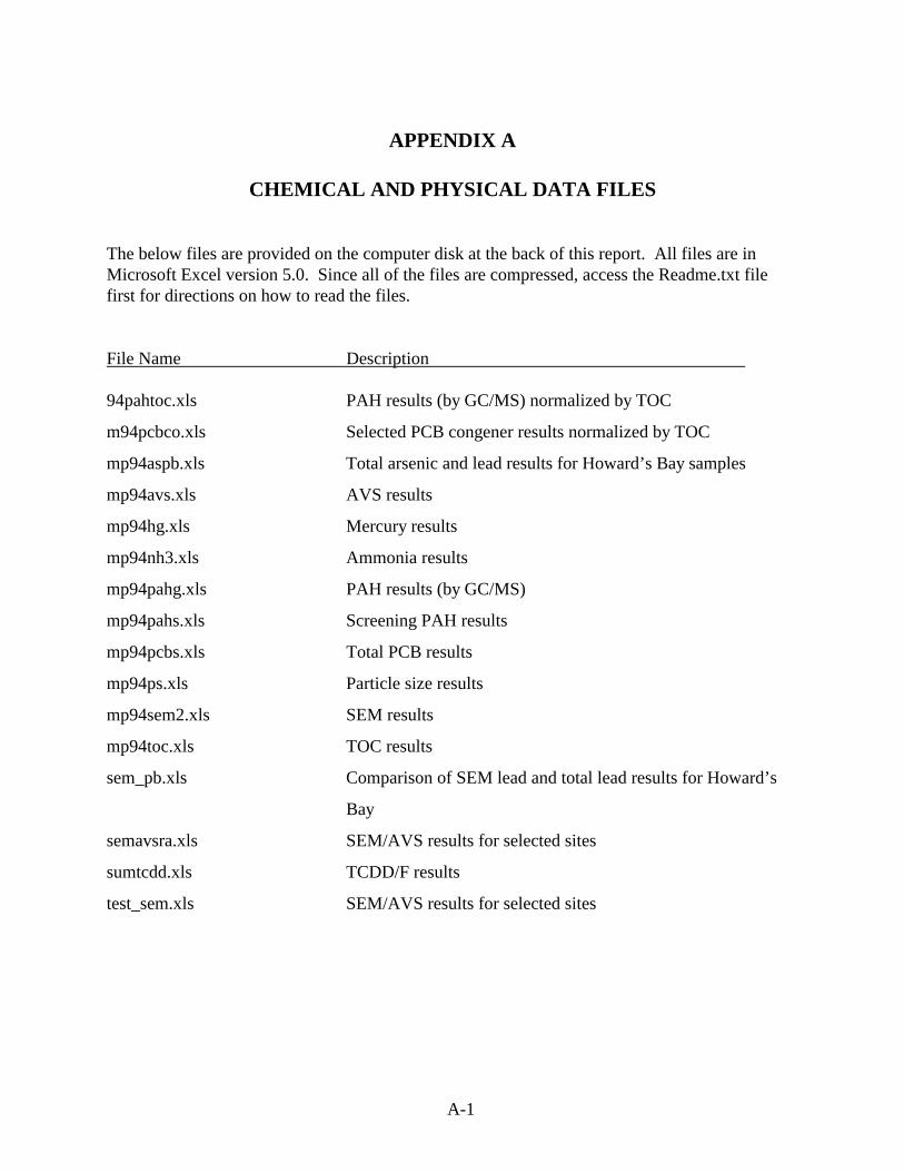
A-1

APPENDIX A

CHEMICAL AND PHYSICAL DATA FILES

The below files are provided on the computer disk at the back of this report. All files are inMicrosoft Excel version 5.0. Since all of the files are compressed, access the Readme.txt filefirst for directions on how to read the files.

File Name Description

94pahtoc.xls PAH results (by GC/MS) normalized by TOC

m94pcbco.xls Selected PCB congener results normalized by TOC

mp94aspb.xls Total arsenic and lead results for Howard’s Bay samples

mp94avs.xls AVS results

mp94hg.xls Mercury results

mp94nh3.xls Ammonia results

mp94pahg.xls PAH results (by GC/MS)

mp94pahs.xls Screening PAH results

mp94pcbs.xls Total PCB results

mp94ps.xls Particle size results

mp94sem2.xls SEM results

mp94toc.xls TOC results

sem_pb.xls Comparison of SEM lead and total lead results for Howard’s

Bay

semavsra.xls SEM/AVS results for selected sites

sumtcdd.xls TCDD/F results

test_sem.xls SEM/AVS results for selected sites

APPENDIX B

SEDIMENT TOXICITY TEST REPORTS

FOR HYALELLA AZTECA AND CHIRONOMUS TENTANS

ACUTE TOXICITY TESTSWITH

HYALELLA AZTECA AND CHIRONOMUS TENTANSON SEDIMENTS FROM THE DULUTH/SUPERIOR HARBOR:

1994 Sampling Results - Batch # 1

Conducted by

Minnesota Pollution Control AgencyMonitoring and Assessment Section

520 Lafayette RoadSt. Paul, Minnesota 55155-4194

April 1997

ii

TABLE OF CONTENTS

INTRODUCTION . . . . . . . . . . . . . . . . . . . . . . . . . . . . . . . . . . . . . . . . . . . . . . . . . . . . . . . . . . . . 1

SAMPLE COLLECTION AND HANDLING . . . . . . . . . . . . . . . . . . . . . . . . . . . . . . . . . . . . . . 1

METHODS .. . . . . . . . . . . . . . . . . . . . . . . . . . . . . . . . . . . . . . . . . . . . . . . . . . . . . . . . . . . . . . . . 1

RESULTS . . . . . . . . . . . . . . . . . . . . . . . . . . . . . . . . . . . . . . . . . . . . . . . . . . . . . . . . . . . . . . . . . . 2

SUMMARY. . . . . . . . . . . . . . . . . . . . . . . . . . . . . . . . . . . . . . . . . . . . . . . . . . . . . . . . . . . . . . . . . .4

REFERENCES . . . . . . . . . . . . . . . . . . . . . . . . . . . . . . . . . . . . . . . . . . . . . . . . . . . . . . . . . . . . . . . 4

APPENDIX A - Statistical Analyses

iii

LIST OF TABLES

TABLE 1. Daily Overlying Water pH Measurements ..................................................................5

TABLE 2. Daily Overlying Water Dissolved Oxygen Concentrations (mg/L)............................. 6

TABLE 3. Daily Overlying Water Temperatures (Degrees Celsius)............................................ 7

TABLE 4. Mean Percent Survival of Hyalella azteca and Chironomus tentans .......................... 8

1

INTRODUCTION

As part of a sediment assessment of hotspot areas in the Duluth/Superior Harbor, sedimenttoxicity tests were conducted to assess acute (survival) and chronic (growth) toxicity to benthicinvertebrates. Acute effects were measured in separate 10-day toxicity tests to Hyalella azteca(H. azteca) and Chironomus tentans (C. tentans). Growth was measured at the end of theC. tentans test to assess chronic effects. Survival and growth endpoints were compared toorganisms similarly exposed to a reference control sediment collected from West Bearskin Lake(Cook County, MN).

A total of 44 sediment samples were collected for toxicity testing. This report presents theresults of seven of these sediment samples.

SAMPLE COLLECTION AND HANDLING

During August 22-24, 1994, Minnesota Pollution Control Agency (MPCA) staff collected theseven sediments referred to in this report. The composited samples were collected from theharbor using a gravity corer. The samples were stored at 4°C at the Duluth MPCA office untilthey were transported to the MPCA Toxicology Laboratory in St. Paul, MN.

METHODS

Seven sediment samples and a control sediment were subjected to 10-day sediment toxicity testsusing the procedures described in U.S. EPA (1994). The test organisms (H. azteca and C.tentans) were exposed to sediment samples in a portable, mini-flow system described in Benoitet al. (1993) and U.S. EPA (1994). The test apparatus consists of 300 mL, glass-beaker testchambers held in a glass box supplied with water from an acrylic plastic headbox. The beakershave two, 1.5 cm holes covered with stainless steel mesh, to allow for water exchange whilecontaining the test organisms. The headbox has a pipette tip drain calibrated to deliver water atan average rate of 32.5 mL/min. The glass box is fitted with a self-starting siphon to provideexchange of overlying water.

The H. azteca used for this test were 1 to 3 mm long, and the C. tentans were approximately 14days old. These organisms were supplied by Environmental Consulting and Testing in Superior,WI. On the test set up day, MPCA personnel picked up the organisms from the supplier andtransported them to the MPCA Toxicology Laboratory.

On September 13, 1994, seven samples (DMIR 03, DMIR 04, MLH 01, MLH 02, MLH 03,MLH 04, and MLH 05) and the control sediment were separately homogenized by hand, and 100mL of each sediment was placed in a test beaker (Batch #1). Each sediment test was set up withfour replicates of H. azteca and four replicates of C. tentans. Approximately 100 mL of aerated,artesian well water was added to the beakers, and the sediments were allowed to settle forapproximately two hours before the organisms were added. For each sediment, ten organismswere placed in each of eight beakers in a random fashion.

2

The organisms were exposed to 16 hours of light and eight hours of darkness for the duration ofthe ten-day test. Each day, two liters of aerated water from the artesian well at Stroh Brewery inSt. Paul, MN were exchanged in each test chamber. On weekdays, 1-L was exchanged in themorning and 1-L in the afternoon. On weekends, the two liters were passed through thechambers all at once. Water quality measurements (i.e., pH, temperature, and dissolved oxygen)of the overlying water were taken in one beaker of each of the quadruplicate sets of each of thesediments. The results, along with daily observations involving the physical appearance of thesediments and organisms, were recorded in a laboratory notebook. This notebook is retained onfile at the MPCA.

The test was terminated on September 23, 1994. The sediments were sieved through 40 meshscreens, and the sieved material was sorted for organisms. The organisms found were counted,and the number of alive and dead organisms were recorded. Organisms not found were recordedas missing and presumed dead. The C. tentans that survived were placed in aluminum weighingdishes, dried at approximately 110°C for at least four hours, desiccated to room temperature, andweighed.

Growth (weight) of the C. tentans and survival of both organisms were used as the endpoints forthese tests. The resulting survival data were analyzed using TOXSTAT (Gulley and WEST, Inc.,1994), a statistical software package obtained from the University of Wyoming. However, due toa quality assurance problem, the growth data were not analyzed.

A 96-hour, reference toxicant test with H. azteca in sodium chloride (NaCl) was run inconjunction with these toxicity tests to determine the acceptability of the H. azteca used. Fourconcentrations of NaCl solution (i.e., 10, 5, 2.5, and 1.25 g/L) and a control (aerated, artesianwell water) were used in this test. Due to a shortage of test organisms, only two replicates of fiveorganisms each were set up per concentration instead of three replicates.

RESULTS

Water Quality

Measurements of pH, dissolved oxygen concentration, and temperature in the overlying water ofthe test beakers were made daily. These measurements are summarized below and in Tables 1, 2,and 3, respectively.

The range of pH values in the beakers containing H. azteca was 7.8 to 9.0 (Table 1). The waterin the C. tentans beakers had a pH range of 7.6 to 8.4 (Table 1). The pH fluctuations duringthese tests were acceptable since they did not vary more than 50% within each treatment (U.S.EPA, 1994).

The dissolved oxygen concentration ranged from 4.5 to 6.5 mg/L in the H. azteca beakers andfrom 2.4 to 6.5 mg/L in the C. tentans beakers (Table 2). All dissolved oxygen concentrationswere within acceptable limits (i.e., greater than 40% saturated).

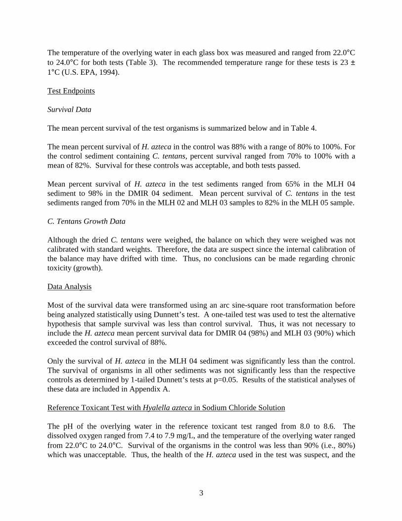
3

The temperature of the overlying water in each glass box was measured and ranged from 22.0°Cto 24.0°C for both tests (Table 3). The recommended temperature range for these tests is 23 ±1°C (U.S. EPA, 1994).

Test Endpoints

Survival Data

The mean percent survival of the test organisms is summarized below and in Table 4.

The mean percent survival of H. azteca in the control was 88% with a range of 80% to 100%. Forthe control sediment containing C. tentans, percent survival ranged from 70% to 100% with amean of 82%. Survival for these controls was acceptable, and both tests passed.

Mean percent survival of H. azteca in the test sediments ranged from 65% in the MLH 04sediment to 98% in the DMIR 04 sediment. Mean percent survival of C. tentans in the testsediments ranged from 70% in the MLH 02 and MLH 03 samples to 82% in the MLH 05 sample.

C. Tentans Growth Data

Although the dried C. tentans were weighed, the balance on which they were weighed was notcalibrated with standard weights. Therefore, the data are suspect since the internal calibration ofthe balance may have drifted with time. Thus, no conclusions can be made regarding chronictoxicity (growth).

Data Analysis

Most of the survival data were transformed using an arc sine-square root transformation beforebeing analyzed statistically using Dunnett’s test. A one-tailed test was used to test the alternativehypothesis that sample survival was less than control survival. Thus, it was not necessary toinclude the H. azteca mean percent survival data for DMIR 04 (98%) and MLH 03 (90%) whichexceeded the control survival of 88%.

Only the survival of H. azteca in the MLH 04 sediment was significantly less than the control.The survival of organisms in all other sediments was not significantly less than the respectivecontrols as determined by 1-tailed Dunnett’s tests at p=0.05. Results of the statistical analyses ofthese data are included in Appendix A.

Reference Toxicant Test with Hyalella azteca in Sodium Chloride Solution

The pH of the overlying water in the reference toxicant test ranged from 8.0 to 8.6. Thedissolved oxygen ranged from 7.4 to 7.9 mg/L, and the temperature of the overlying water rangedfrom 22.0°C to 24.0°C. Survival of the organisms in the control was less than 90% (i.e., 80%)which was unacceptable. Thus, the health of the H. azteca used in the test was suspect, and the

4

test failed. The test was also suspect due to an inadequate number of replicates (i.e., tworeplicates instead of three) used in the test.

SUMMARY

Survival of H. azteca in the control sediments was acceptable (i.e., greater than 80%), andsample MLH 04 caused significant toxicity to H. azteca (p=0.05). Although the referencetoxicant test failed, the health of the culture appeared to be acceptable for use in the toxicity test.

Control survival was acceptable in the C. tentans test (i.e., greater than 70%), and none of the testsediments resulted in significantly lower survival of C. tentans when compared to the controlsurvival (p = 0.05).

REFERENCES

Benoit, D.A., G. Phipps, and G.T. Ankley. 1993. A sediment testing intermittent renewal system for the automated renewal of overlying water in toxicity tests with contaminated sediments. Water Research 27:1403-1412.

Gulley, D.D. and WEST, Inc. 1994. TOXSTAT 3.4. WEST, Inc., Cheyenne, WY.

U.S. EPA. 1994. Methods for measuring the toxicity and bioaccumulation of sediment-associated contaminants with freshwater invertebrates. Office of Research and Development, U.S. Environmental Protection Agency, Duluth, MN. EPA/600/R-94/024.

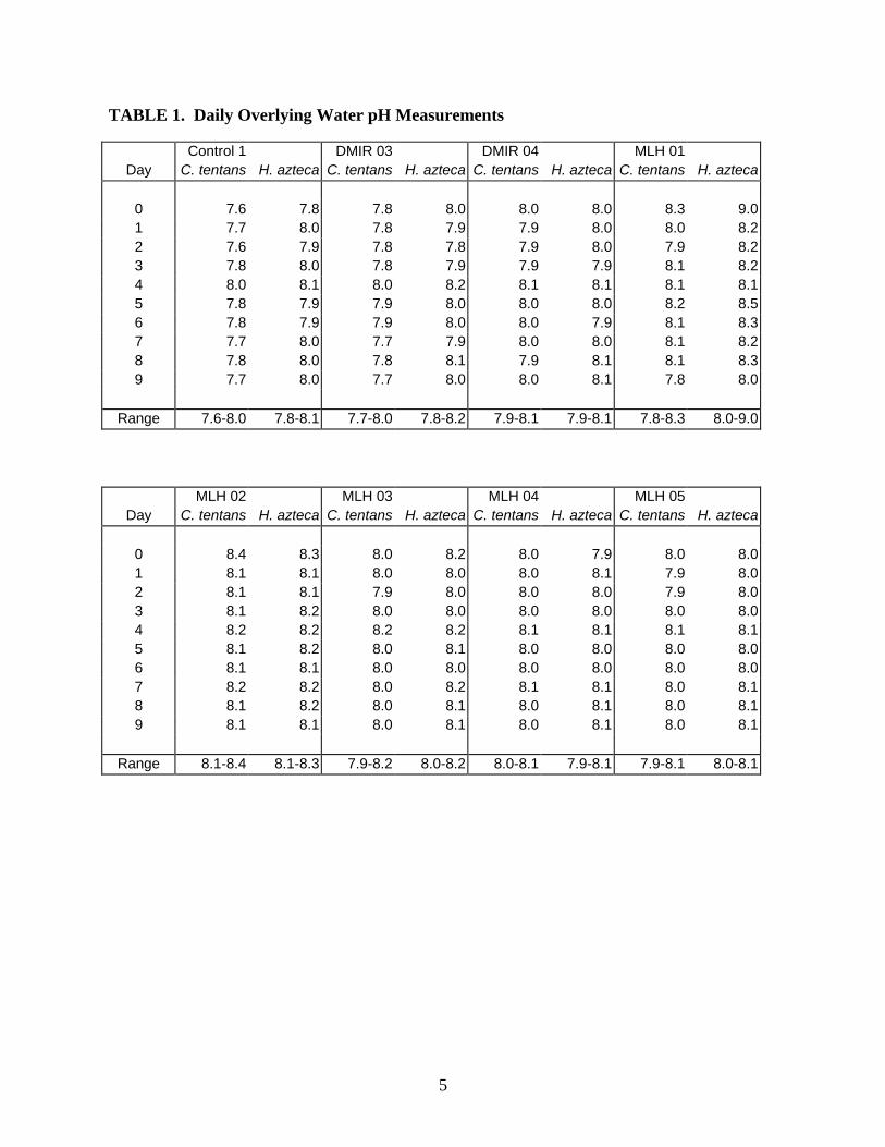
5

TABLE 1. Daily Overlying Water pH Measurements

Control 1 DMIR 03 DMIR 04 MLH 01Day C. tentans H. azteca C. tentans H. azteca C. tentans H. azteca C. tentans H. azteca

0 7.6 7.8 7.8 8.0 8.0 8.0 8.3 9.01 7.7 8.0 7.8 7.9 7.9 8.0 8.0 8.22 7.6 7.9 7.8 7.8 7.9 8.0 7.9 8.23 7.8 8.0 7.8 7.9 7.9 7.9 8.1 8.24 8.0 8.1 8.0 8.2 8.1 8.1 8.1 8.15 7.8 7.9 7.9 8.0 8.0 8.0 8.2 8.56 7.8 7.9 7.9 8.0 8.0 7.9 8.1 8.37 7.7 8.0 7.7 7.9 8.0 8.0 8.1 8.28 7.8 8.0 7.8 8.1 7.9 8.1 8.1 8.39 7.7 8.0 7.7 8.0 8.0 8.1 7.8 8.0

Range 7.6-8.0 7.8-8.1 7.7-8.0 7.8-8.2 7.9-8.1 7.9-8.1 7.8-8.3 8.0-9.0

MLH 02 MLH 03 MLH 04 MLH 05Day C. tentans H. azteca C. tentans H. azteca C. tentans H. azteca C. tentans H. azteca

0 8.4 8.3 8.0 8.2 8.0 7.9 8.0 8.01 8.1 8.1 8.0 8.0 8.0 8.1 7.9 8.02 8.1 8.1 7.9 8.0 8.0 8.0 7.9 8.03 8.1 8.2 8.0 8.0 8.0 8.0 8.0 8.04 8.2 8.2 8.2 8.2 8.1 8.1 8.1 8.15 8.1 8.2 8.0 8.1 8.0 8.0 8.0 8.06 8.1 8.1 8.0 8.0 8.0 8.0 8.0 8.07 8.2 8.2 8.0 8.2 8.1 8.1 8.0 8.18 8.1 8.2 8.0 8.1 8.0 8.1 8.0 8.19 8.1 8.1 8.0 8.1 8.0 8.1 8.0 8.1

Range 8.1-8.4 8.1-8.3 7.9-8.2 8.0-8.2 8.0-8.1 7.9-8.1 7.9-8.1 8.0-8.1

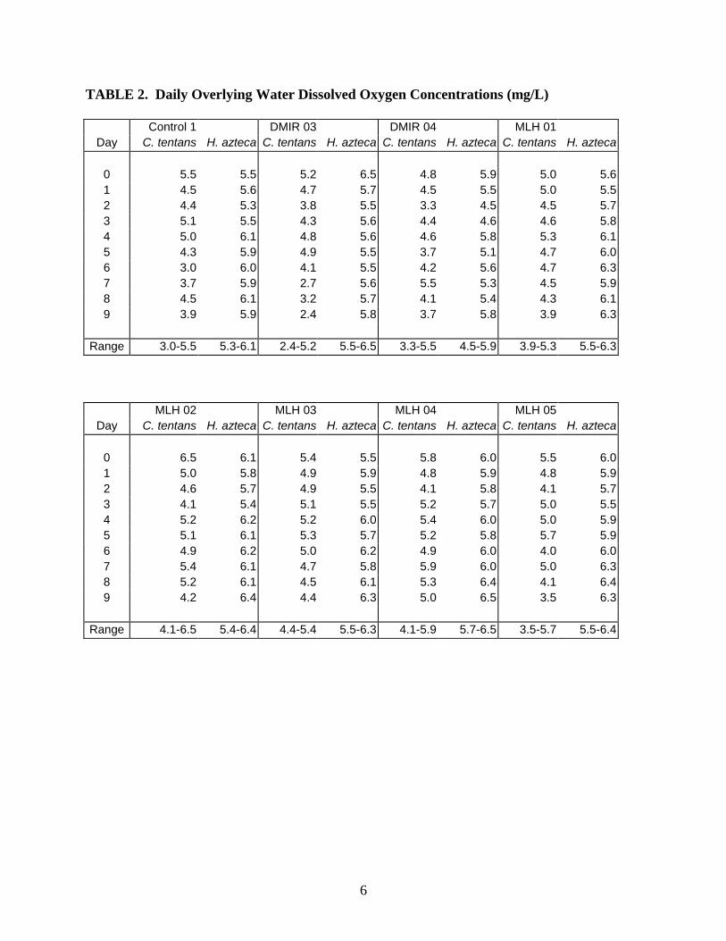
6

TABLE 2. Daily Overlying Water Dissolved Oxygen Concentrations (mg/L)

Control 1 DMIR 03 DMIR 04 MLH 01Day C. tentans H. azteca C. tentans H. azteca C. tentans H. azteca C. tentans H. azteca

0 5.5 5.5 5.2 6.5 4.8 5.9 5.0 5.61 4.5 5.6 4.7 5.7 4.5 5.5 5.0 5.52 4.4 5.3 3.8 5.5 3.3 4.5 4.5 5.73 5.1 5.5 4.3 5.6 4.4 4.6 4.6 5.84 5.0 6.1 4.8 5.6 4.6 5.8 5.3 6.15 4.3 5.9 4.9 5.5 3.7 5.1 4.7 6.06 3.0 6.0 4.1 5.5 4.2 5.6 4.7 6.37 3.7 5.9 2.7 5.6 5.5 5.3 4.5 5.98 4.5 6.1 3.2 5.7 4.1 5.4 4.3 6.19 3.9 5.9 2.4 5.8 3.7 5.8 3.9 6.3

Range 3.0-5.5 5.3-6.1 2.4-5.2 5.5-6.5 3.3-5.5 4.5-5.9 3.9-5.3 5.5-6.3

MLH 02 MLH 03 MLH 04 MLH 05Day C. tentans H. azteca C. tentans H. azteca C. tentans H. azteca C. tentans H. azteca

0 6.5 6.1 5.4 5.5 5.8 6.0 5.5 6.01 5.0 5.8 4.9 5.9 4.8 5.9 4.8 5.92 4.6 5.7 4.9 5.5 4.1 5.8 4.1 5.73 4.1 5.4 5.1 5.5 5.2 5.7 5.0 5.54 5.2 6.2 5.2 6.0 5.4 6.0 5.0 5.95 5.1 6.1 5.3 5.7 5.2 5.8 5.7 5.96 4.9 6.2 5.0 6.2 4.9 6.0 4.0 6.07 5.4 6.1 4.7 5.8 5.9 6.0 5.0 6.38 5.2 6.1 4.5 6.1 5.3 6.4 4.1 6.49 4.2 6.4 4.4 6.3 5.0 6.5 3.5 6.3

Range 4.1-6.5 5.4-6.4 4.4-5.4 5.5-6.3 4.1-5.9 5.7-6.5 3.5-5.7 5.5-6.4

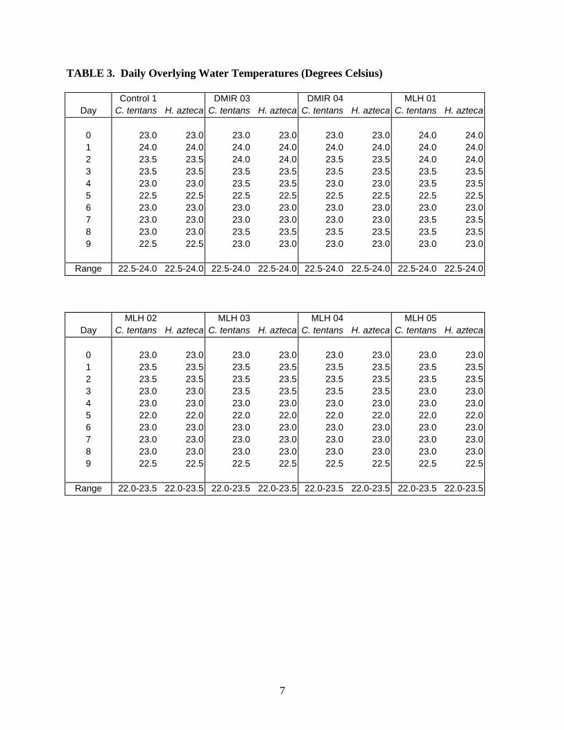
7

TABLE 3. Daily Overlying Water Temperatures (Degrees Celsius)

Control 1 DMIR 03 DMIR 04 MLH 01Day C. tentans H. azteca C. tentans H. azteca C. tentans H. azteca C. tentans H. azteca

0 23.0 23.0 23.0 23.0 23.0 23.0 24.0 24.01 24.0 24.0 24.0 24.0 24.0 24.0 24.0 24.02 23.5 23.5 24.0 24.0 23.5 23.5 24.0 24.03 23.5 23.5 23.5 23.5 23.5 23.5 23.5 23.54 23.0 23.0 23.5 23.5 23.0 23.0 23.5 23.55 22.5 22.5 22.5 22.5 22.5 22.5 22.5 22.56 23.0 23.0 23.0 23.0 23.0 23.0 23.0 23.07 23.0 23.0 23.0 23.0 23.0 23.0 23.5 23.58 23.0 23.0 23.5 23.5 23.5 23.5 23.5 23.59 22.5 22.5 23.0 23.0 23.0 23.0 23.0 23.0

Range 22.5-24.0 22.5-24.0 22.5-24.0 22.5-24.0 22.5-24.0 22.5-24.0 22.5-24.0 22.5-24.0

MLH 02 MLH 03 MLH 04 MLH 05Day C. tentans H. azteca C. tentans H. azteca C. tentans H. azteca C. tentans H. azteca

0 23.0 23.0 23.0 23.0 23.0 23.0 23.0 23.01 23.5 23.5 23.5 23.5 23.5 23.5 23.5 23.52 23.5 23.5 23.5 23.5 23.5 23.5 23.5 23.53 23.0 23.0 23.5 23.5 23.5 23.5 23.0 23.04 23.0 23.0 23.0 23.0 23.0 23.0 23.0 23.05 22.0 22.0 22.0 22.0 22.0 22.0 22.0 22.06 23.0 23.0 23.0 23.0 23.0 23.0 23.0 23.07 23.0 23.0 23.0 23.0 23.0 23.0 23.0 23.08 23.0 23.0 23.0 23.0 23.0 23.0 23.0 23.09 22.5 22.5 22.5 22.5 22.5 22.5 22.5 22.5

Range 22.0-23.5 22.0-23.5 22.0-23.5 22.0-23.5 22.0-23.5 22.0-23.5 22.0-23.5 22.0-23.5

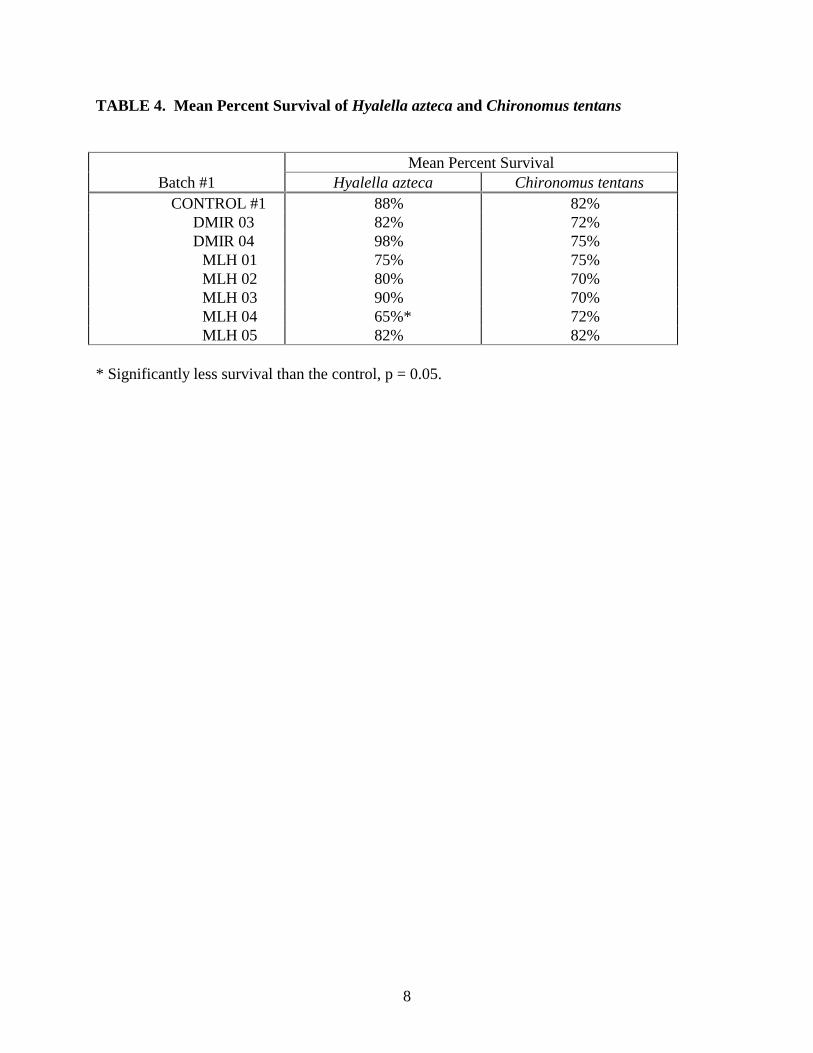
8

TABLE 4. Mean Percent Survival of Hyalella azteca and Chironomus tentans

Mean Percent SurvivalBatch #1 Hyalella azteca Chironomus tentans

CONTROL #1 88% 82%DMIR 03 82% 72%DMIR 04 98% 75%

MLH 01 75% 75%MLH 02 80% 70%MLH 03 90% 70%MLH 04 65%* 72%MLH 05 82% 82%

* Significantly less survival than the control, p = 0.05.

APPENDIX A

Statistical Analyses

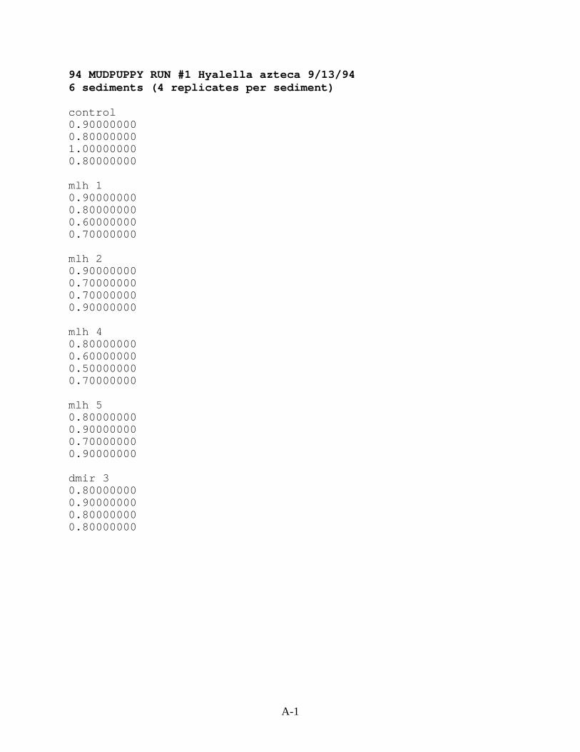
A-1

94 MUDPUPPY RUN #1 Hyalella azteca 9/13/946 sediments (4 replicates per sediment)

control0.900000000.800000001.000000000.80000000

mlh 10.900000000.800000000.600000000.70000000

mlh 20.900000000.700000000.700000000.90000000

mlh 40.800000000.600000000.500000000.70000000

mlh 50.800000000.900000000.700000000.90000000

dmir 30.800000000.900000000.800000000.80000000

A-2

TITLE: 94 MUDPUPPY RUN #1 Hyalella azteca 9/13/94FILE: 94MUD1.DATTRANSFORM: ARC SINE(SQUARE ROOT(Y)) NUMBER OFGROUPS: 6----------------------------------------------------------------------

GRP IDENTIFICATION REP VALUE TRANS VALUE--- ---------------- ---- ------------- -------------1 control 1 0.9000 1.24901 control 2 0.8000 1.10711 control 3 1.0000 1.41201 control 4 0.8000 1.10712 mlh 1 1 0.9000 1.24902 mlh 1 2 0.8000 1.10712 mlh 1 3 0.6000 0.88612 mlh 1 4 0.7000 0.99123 mlh 2 1 0.9000 1.24903 mlh 2 2 0.7000 0.99123 mlh 2 3 0.7000 0.99123 mlh 2 4 0.9000 1.24904 mlh 4 1 0.8000 1.10714 mlh 4 2 0.6000 0.88614 mlh 4 3 0.5000 0.78544 mlh 4 4 0.7000 0.99125 mlh 5 1 0.8000 1.10715 mlh 5 2 0.9000 1.24905 mlh 5 3 0.7000 0.99125 mlh 5 4 0.9000 1.24906 dmir 3 1 0.8000 1.10716 dmir 3 2 0.9000 1.24906 dmir 3 3 0.8000 1.10716 dmir 3 4 0.8000 1.1071----------------------------------------------------------------------

A-3

94 MUDPUPPY RUN #1 Hyalella azteca 9/13/94File: 94MUD1.DAT Transform: ARC SINE(SQUARE ROOT(Y))

SUMMARY STATISTICS ON TRANSFORMED DATA TABLE 1 of 2------------------------------------------------------------------------

GRP IDENTIFICATION N MIN MAX MEAN--- ---------------- ---- ---------- ---------- ----------1 control 4 1.107 1.412 1.2192 mlh 1 4 0.886 1.249 1.0583 mlh 2 4 0.991 1.249 1.1204 mlh 4 4 0.785 1.107 0.9425 mlh 5 4 0.991 1.249 1.1496 dmir 3 4 1.107 1.249 1.143------------------------------------------------------------------------

94 MUDPUPPY RUN #1 Hyalella azteca 9/13/94File: 94MUD1.DAT Transform: ARC SINE(SQUARE ROOT(Y))

SUMMARY STATISTICS ON TRANSFORMED DATA TABLE 2 of 2------------------------------------------------------------------------

GRP IDENTIFICATION VARIANCE SD SEM C.V. %--- ---------------- -------------- ---------- ---------- ----------1 control 0.021 0.145 0.073 11.912 mlh 1 0.024 0.156 0.078 14.733 mlh 2 0.022 0.149 0.074 13.294 mlh 4 0.019 0.138 0.069 14.675 mlh 5 0.016 0.125 0.062 10.866 dmir 3 0.005 0.071 0.035 6.21------------------------------------------------------------------------

A-4

94 MUDPUPPY RUN #1 Hyalella azteca 9/13/94File: 94MUD1.DAT Transform: ARC SINE(SQUARE ROOT(Y))

Shapiro - Wilk's test for normality----------------------------------------------------------------------

D = 0.322

W = 0.931

Critical W (P = 0.05) (n = 24) = 0.916Critical W (P = 0.01) (n = 24) = 0.884----------------------------------------------------------------------

Data PASS normality test at P=0.01 level. Continue analysis.

94 MUDPUPPY RUN #1 Hyalella azteca 9/13/94File: 94MUD1.DAT Transform: ARC SINE(SQUARE ROOT(Y))

----------------------------------------------------------------------Bartlett's test for homogeneity of varianceCalculated B1 statistic = 1.73

----------------------------------------------------------------------Table Chi-square value = 15.09 (alpha = 0.01, df = 5)Table Chi-square value = 11.07 (alpha = 0.05, df = 5)

Data PASS B1 homogeneity test at 0.01 level. Continue analysis.

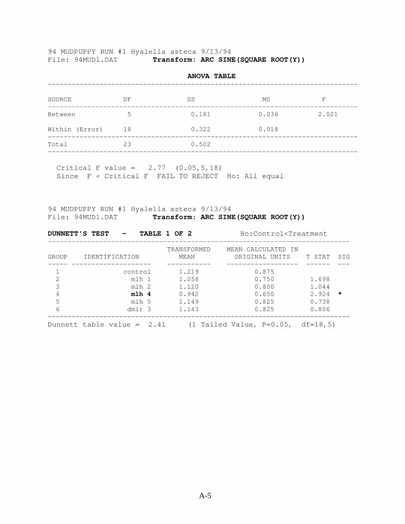
A-5

94 MUDPUPPY RUN #1 Hyalella azteca 9/13/94File: 94MUD1.DAT Transform: ARC SINE(SQUARE ROOT(Y))

ANOVA TABLE------------------------------------------------------------------------------

SOURCE DF SS MS F------------------------------------------------------------------------------Between 5 0.181 0.036 2.021

Within (Error) 18 0.322 0.018------------------------------------------------------------------------------Total 23 0.502------------------------------------------------------------------------------

Critical F value = 2.77 (0.05,5,18)Since F < Critical F FAIL TO REJECT Ho: All equal

94 MUDPUPPY RUN #1 Hyalella azteca 9/13/94File: 94MUD1.DAT Transform: ARC SINE(SQUARE ROOT(Y))

DUNNETT'S TEST - TABLE 1 OF 2 Ho:Control<Treatment----------------------------------------------------------------------------

TRANSFORMED MEAN CALCULATED INGROUP IDENTIFICATION MEAN ORIGINAL UNITS T STAT SIG----- -------------------- ----------- ------------------ ------ ---

1 control 1.219 0.8752 mlh 1 1.058 0.750 1.6983 mlh 2 1.120 0.800 1.0444 mlh 4 0.942 0.650 2.924 *5 mlh 5 1.149 0.825 0.7386 dmir 3 1.143 0.825 0.806

----------------------------------------------------------------------------Dunnett table value = 2.41 (1 Tailed Value, P=0.05, df=18,5)

A-6

94 MUDPUPPY RUN #1 Hyalella azteca 9/13/94File: 94MUD1.DAT Transform: ARC SINE(SQUARE ROOT(Y))

DUNNETT'S TEST - TABLE 2 OF 2 Ho:Control<Treatment----------------------------------------------------------------------------

NUM OF Minimum Sig Diff % of DIFFERENCEGROUP IDENTIFICATION REPS (IN ORIG. UNITS) CONTROL FROM CONTROL----- -------------------- ------- ---------------- ------- ------------

1 control 42 mlh 1 4 0.181 20.7 0.1253 mlh 2 4 0.181 20.7 0.0754 mlh 4 4 0.181 20.7 0.2255 mlh 5 4 0.181 20.7 0.0506 dmir 3 4 0.181 20.7 0.050

------------------------------------------------------------------------------

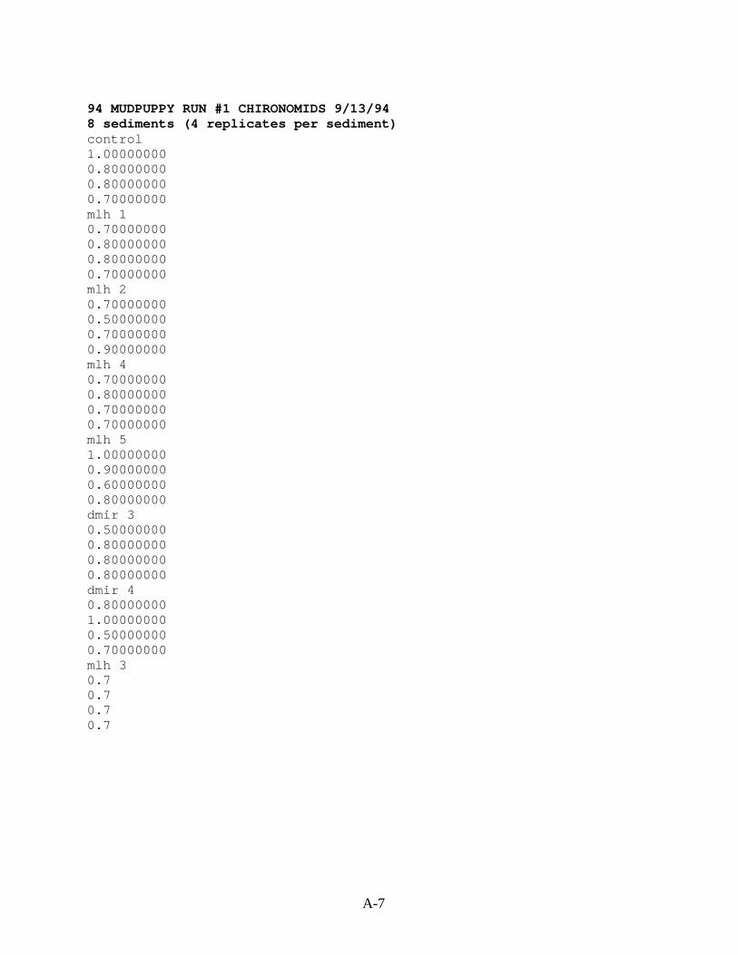
A-7

94 MUDPUPPY RUN #1 CHIRONOMIDS 9/13/948 sediments (4 replicates per sediment)control1.000000000.800000000.800000000.70000000mlh 10.700000000.800000000.800000000.70000000mlh 20.700000000.500000000.700000000.90000000mlh 40.700000000.800000000.700000000.70000000mlh 51.000000000.900000000.600000000.80000000dmir 30.500000000.800000000.800000000.80000000dmir 40.800000001.000000000.500000000.70000000mlh 30.70.70.70.7

A-8

TITLE: 94 MUDPUPPY RUN #1 CHIRONOMIDS 9/13/94FILE: 94MUD1ch.DATTRANSFORM: ARC SINE(SQUARE ROOT(Y)) NUMBER OF GROUPS: 8----------------------------------------------------------------------

GRP IDENTIFICATION REP VALUE TRANS VALUE--- ---------------- ---- ------------- -------------1 control 1 1.0000 1.41201 control 2 0.8000 1.10711 control 3 0.8000 1.10711 control 4 0.7000 0.99122 mlh 1 1 0.7000 0.99122 mlh 1 2 0.8000 1.10712 mlh 1 3 0.8000 1.10712 mlh 1 4 0.7000 0.99123 mlh 2 1 0.7000 0.99123 mlh 2 2 0.5000 0.78543 mlh 2 3 0.7000 0.99123 mlh 2 4 0.9000 1.24904 mlh 4 1 0.7000 0.99124 mlh 4 2 0.8000 1.10714 mlh 4 3 0.7000 0.99124 mlh 4 4 0.7000 0.99125 mlh 5 1 1.0000 1.41205 mlh 5 2 0.9000 1.24905 mlh 5 3 0.6000 0.88615 mlh 5 4 0.8000 1.10716 dmir 3 1 0.5000 0.78546 dmir 3 2 0.8000 1.10716 dmir 3 3 0.8000 1.10716 dmir 3 4 0.8000 1.10717 dmir 4 1 0.8000 1.10717 dmir 4 2 1.0000 1.41207 dmir 4 3 0.5000 0.78547 dmir 4 4 0.7000 0.99128 mlh 3 1 0.7000 0.99128 mlh 3 2 0.7000 0.99128 mlh 3 3 0.7000 0.99128 mlh 3 4 0.7000 0.9912----------------------------------------------------------------------

A-9

94 MUDPUPPY RUN #1 CHIRONOMIDS 9/13/94File: 94MUD1ch.DAT Transform: ARC SINE(SQUARE ROOT(Y))

SUMMARY STATISTICS ON TRANSFORMED DATA TABLE 1 of 2----------------------------------------------------------------------

GRP IDENTIFICATION N MIN MAX MEAN--- ---------------- ---- ---------- ---------- ----------1 control 4 0.991 1.412 1.1542 mlh 1 4 0.991 1.107 1.0493 mlh 2 4 0.785 1.249 1.0044 mlh 4 4 0.991 1.107 1.0205 mlh 5 4 0.886 1.412 1.1646 dmir 3 4 0.785 1.107 1.0277 dmir 4 4 0.785 1.412 1.0748 mlh 3 4 0.991 0.991 0.991----------------------------------------------------------------------

94 MUDPUPPY RUN #1 CHIRONOMIDS 9/13/94File: 94MUD1ch.DAT Transform: ARC SINE(SQUARE ROOT(Y))

SUMMARY STATISTICS ON TRANSFORMED DATA TABLE 2 of 2------------------------------------------------------------------------

GRP IDENTIFICATION VARIANCE SD SEM C.V. %--- ---------------- -------------- ---------- ---------- ----------1 control 0.032 0.180 0.090 15.622 mlh 1 0.004 0.067 0.033 6.383 mlh 2 0.036 0.190 0.095 18.914 mlh 4 0.003 0.058 0.029 5.695 mlh 5 0.050 0.223 0.112 19.176 dmir 3 0.026 0.161 0.080 15.677 dmir 4 0.069 0.262 0.131 24.378 mlh 3 0.000 0.000 0.000 0.00------------------------------------------------------------------------

A-10

94 MUDPUPPY RUN #1 CHIRONOMIDS 9/13/94File: 94MUD1ch.DAT Transform: ARC SINE(SQUARE ROOT(Y))

Shapiro - Wilk's test for normality----------------------------------------------------------------------

D = 0.662

W = 0.942

Critical W (P = 0.05) (n = 32) = 0.930Critical W (P = 0.01) (n = 32) = 0.904----------------------------------------------------------------------

Data PASS normality test at P=0.01 level. Continue analysis.

94 MUDPUPPY RUN #1 CHIRONOMIDS 9/13/94File: 94MUD1ch.DAT Transform: ARC SINE(SQUARE ROOT(Y))

Hartley's test for homogeneity of varianceBartlett's test for homogeneity of variance----------------------------------------------------------------------

These two tests can not be performed because at least one group haszero variance.

Data FAIL to meet homogeneity of variance assumption.Additional transformations are useless.

----------------------------------------------------------------------

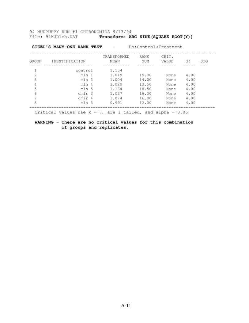
A-11

94 MUDPUPPY RUN #1 CHIRONOMIDS 9/13/94File: 94MUD1ch.DAT Transform: ARC SINE(SQUARE ROOT(Y))

STEEL'S MANY-ONE RANK TEST - Ho:Control<Treatment----------------------------------------------------------------------------

TRANSFORMED RANK CRIT.GROUP IDENTIFICATION MEAN SUM VALUE df SIG----- -------------------- ----------- ------- ------ ----- ---

1 control 1.1542 mlh 1 1.049 15.00 None 4.003 mlh 2 1.004 14.00 None 4.004 mlh 4 1.020 13.50 None 4.005 mlh 5 1.164 18.50 None 4.006 dmir 3 1.027 16.00 None 4.007 dmir 4 1.074 16.00 None 4.008 mlh 3 0.991 12.00 None 4.00

----------------------------------------------------------------------------Critical values use k = 7, are 1 tailed, and alpha = 0.05

WARNING - There are no critical values for this combinationof groups and replicates.

ACUTE TOXICITY TESTSWITH

HYALELLA AZTECA AND CHIRONOMUS TENTANSON SEDIMENTS FROM THE DULUTH/SUPERIOR HARBOR:

1994 Sampling Results - Batch # 2

Conducted by

Minnesota Pollution Control AgencyMonitoring and Assessment Section

520 Lafayette RoadSt. Paul, Minnesota 55155-4194

April 1997

ii

TABLE OF CONTENTS

INTRODUCTION . . . . . . . . . . . . . . . . . . . . . . . . . . . . . . . . . . . . . . . . . . . . . . . . . . . . . . . . . . . . 1

SAMPLE COLLECTION AND HANDLING . . . . . . . . . . . . . . . . . . . . . . . . . . . . . . . . . . . . . . 1

METHODS .. . . . . . . . . . . . . . . . . . . . . . . . . . . . . . . . . . . . . . . . . . . . . . . . . . . . . . . . . . . . . . . . 1

RESULTS . . . . . . . . . . . . . . . . . . . . . . . . . . . . . . . . . . . . . . . . . . . . . . . . . . . . . . . . . . . . . . . . . . 2

SUMMARY . . . . . . . . . . . . . . . . . . . . . . . . . . . . . . . . . . . . . . . . . . . . . . . . . . . . . . . . . . . . . . . . 4

REFERENCES . . . . . . . . . . . . . . . . . . . . . . . . . . . . . . . . . . . . . . . . . . . . . . . . . . . . . . . . . . . . . . . 4

APPENDIX A - Statistical Analyses

iii

LIST OF TABLES

TABLE 1. Daily Overlying Water pH Measurements ..................................................................5

TABLE 2. Daily Overlying Water Dissolved Oxygen Concentrations (mg/L) ............................ 6

TABLE 3. Daily Overlying Water Temperatures (Degrees Celsius)............................................ 7

TABLE 4. Mean Percent Survival of Hyalella azteca and Chironomus tentans .......................... 8

1

INTRODUCTION

As part of a sediment assessment of hotspot areas in the Duluth/Superior Harbor, sedimenttoxicity tests were conducted to assess acute (survival) and chronic (growth) toxicity to benthicinvertebrates. Acute effects were measured in separate 10-day toxicity tests to Hyalella azteca(H. azteca) and Chironomus tentans (C. tentans). Growth was measured at the end of theC. tentans test to assess chronic effects. Survival and growth endpoints were compared toorganisms similarly exposed to a reference control sediment collected from West Bearskin Lake(Cook County, MN).

A total of 44 sediment samples were collected for toxicity testing. This report presents theresults of eleven of these sediment samples.

SAMPLE COLLECTION AND HANDLING

During August 23-24, 1994 and September 21-23, 1994, Minnesota Pollution Control Agency(MPCA) staff collected the eleven sediments referred to in this report. The samples werecollected from the harbor using a gravity corer. The samples were stored at 4°C until they weretransported to the MPCA Toxicology Laboratory in St. Paul, MN.

METHODS

Eleven sediment samples and a control sediment were subjected to the 10-day sediment toxicitytest using standard methods for this analysis (U.S. EPA, 1994). The test organisms (H. aztecaand C. tentans) were exposed to sediment samples in a mini-flow system (Benoit et al., 1993;U.S. EPA, 1994). The test apparatus consists of 300 mL, glass-beaker test chambers held in aglass box supplied with water from an acrylic plastic headbox. The beakers have two, 1.5 cmholes covered with stainless steel mesh, to allow for water exchange while containing the testorganisms. The headbox has a pipette tip drain calibrated to deliver water at an average rate of32.5 mL/min. The glass box is fitted with a self-starting siphon to provide exchange of overlyingwater.

The H. azteca used for this test were 1 to 3 mm long, and the C. tentans were approximately 14days old. These organisms were supplied by Environmental Consulting and Testing, Superior,WI prior to the test set up.

On October 4, 1994, eleven samples (DMIR 01, DMIR 02, MLH 06, SUS 01, SUS 03, WLS 01,WLS 02, WLS 03, WLS 04, WLS 06, and WLS 08) and the control sediment were separatelyhomogenized by hand, and 100 mL of each sediment were placed in a test beaker. Each sedimenttest was set up with four replicates of H. azteca and four replicates of C. tentans. Approximately100 mL of aerated artesian well water was added to the beakers, and the sediments were allowedto settle for approximately two hours before the organisms were added. For each sediment, tenorganisms were placed in each of eight beakers in a random fashion.

2

The organisms were exposed to 16 hours of light and eight hours of darkness for the duration ofthe ten-day test. Each day, two liters of aerated water from the artesian well at Stroh Brewery inSt. Paul, MN were exchanged in each test chamber. On weekdays, 1-L was exchanged in themorning and 1-L in the afternoon. On weekends, the two liters were passed through thechambers all at once. Water quality measurements (i.e., pH, temperature, and dissolved oxygen)of the overlying water were taken in one beaker of each of the quadruplicate sets of each of thesediments. The results, along with daily observations involving the physical appearance of thesediments and organisms, were recorded in a laboratory notebook. This notebook is retained onfile at the MPCA.

The test was terminated on October 14, 1994. The sediments were sieved through 40 meshscreens, and the sieved material was sorted for organisms. The organisms found were counted,and the number of alive and dead organisms were recorded. Organisms not found were recordedas missing and presumed dead. The C. tentans that survived were placed in aluminum weighingdishes, dried at approximately 100°C for at least four hours, desiccated to room temperature, andweighed.

Growth (weight) of the C. tentans and survival of both organisms were used as the endpoints forthese tests. The survival data were analyzed using TOXSTAT (Gulley and WEST, Inc., 1994), astatistical software package obtained from the University of Wyoming. However, due to aquality assurance problem, the growth data were not analyzed.

A 96-hour, reference toxicant test with H. azteca in sodium chloride (NaCl) was run inconjunction with these toxicity tests to determine the acceptability of the H. azteca used. Fourconcentrations of NaCl solution (i.e., 10, 5, 2.5, and 1.25 g/L) and a control (aerated, artesianwell water) were used in this test. Three replicates of five organisms each were set up perconcentration.

RESULTS

Water Quality

Measurements of pH, dissolved oxygen, and temperature in the overlying water of the testbeakers were made daily. These measurements are summarized below and in Tables 1, 2, and 3,respectively.

The range of pH values in the beakers containing H. azteca was 7.1 to 8.1 (Table 1). The waterin the C. tentans beakers had a pH range of 6.9 to 8.0 (Table 1). The pH fluctuations duringthese tests were acceptable since they did not vary more than 50% within each treatment (U.S.EPA, 1994).

The dissolved oxygen concentration ranged from 3.7 to 6.4 mg/L in the H. azteca beakers andfrom 1.7 to 6.1 mg/L in the C. tentans beakers (Table 2). All dissolved oxygen concentrationswere within acceptable limits (i.e., greater than 40% saturated).

3

The temperature of the overlying water in each glass box was measured and ranged from 21.5°Cto 23.0°C for both tests (Table 3). The recommended temperature range for these tests is 23 ±1°C (U.S. EPA, 1994).

Test Endpoints

Survival Data

The mean percent survival of the test organisms is summarized below and in Table 4.

The mean percent survival of H. azteca in the control was 92% with a range of 90% to 100%.For the control sediment containing C. tentans, percent survival ranged from 80% to 100% witha mean of 95%. Survival for these controls was acceptable, and both tests passed.

Mean percent survival of H. azteca in the test sediments ranged from 70% in the DMIR 01sediment to 98% in the WLS 04 sediment. Mean percent survival of C. tentans in the testsediments ranged from 55% in the SUS 03 sample to 92% in the MLH 06 sample.

C. Tentans Growth Data

Although the dried C. tentans were weighed, the balance on which they were weighed was notcalibrated with standard weights. Therefore, the data are suspect since the internal calibration ofthe balance may have drifted with time. Thus, no conclusions can be made regarding chronictoxicity (growth).

Data Analysis

Most of the survival data were transformed using an arc sine-square root transformation beforebeing subjected to statistical analysis. A one-tailed test was used to test the alternativehypothesis that sample survival was less than control survival. Thus, it was not necessary toinclude the H. azteca mean percent survival data for DMIR 02 (95%) and WLS 04 (98%) whichexceeded the control survival of 92%. When TOXSTAT was run on the rest of the H. aztecasamples, the data were non-normal due to the survival of the WLS 03 replicates (i.e., 90%, 20%,90%, and 90%). This resulted in Steel’s Many-one Rank test being run on the data set. None ofthe sample survivals were significantly less than the control survival (∝ = 0.05). However,because the replicate survival for WLS 03 was consistently high (i.e., 90%) except for onereplicate (i.e., 20%), this sample was removed from the data set so that a stronger, parametricstatistical analysis could be conducted. When Dunnett’s test was used, DMIR 01 hadsignificantly less H. azteca survival than the corresponding control (p = 0.05).

For C. tentans, Dunnett’s test was used to determine that DMIR 01, SUS 03, and WLS 01 hadsignificantly lower survival than the control (p = 0.05). Results of the statistical analyses ofthese data are included in Appendix A.

4

Reference Toxicant Test with Hyalella azteca in Sodium Chloride Solution

The pH of the overlying water in the reference toxicant test ranged from 7.8 to 8.5. Thedissolved oxygen ranged from 6.4 to 8.3 mg/L, and the temperature of the overlying waterranged from 21.0°C to 22.5°C. Survival of the organisms in the control was less than 90% (i.e.,53%) which was unacceptable. Although two of the control replicates had 100% survival at theend of the test, the third replicate experienced complete mortality of the Hyalella. The reason forthis complete mortality could not be determined. Thus, the test failed.

SUMMARY

Although the survival of H. azteca in the control sediment was acceptable (i.e., greater than80%), the corresponding reference toxicant test failed due to poor control survival in one of thereplicates. The reason for this reference toxicant failure could not be determined. From theH. azteca data that were analyzed statistically, only DMIR 01 had significantly less survival thanthe corresponding control survival (p = 0.05).

Control survival was acceptable in the C. tentans test (i.e., greater than 70%), and only thesurvival of organisms in the DMIR 01, SUS 03, and WLS 01 sediments was significantly lessthan that of the control as determined by a 1-tailed Dunnett’s test (p=0.05).

REFERENCES

Benoit, D.A., G. Phipps, and G.T. Ankley. 1993. A sediment testing intermittent renewal system for the automated renewal of overlying water in toxicity tests with contaminated sediments. Water Research 27:1403-1412.

Gulley, D.D. and WEST, Inc. 1994. TOXSTAT 3.4. WEST, Inc., Cheyenne, WY.

U.S. EPA. 1994. Methods for measuring the toxicity and bioaccumulation of sediment-associated contaminants with freshwater invertebrates. Office of Research and Development, U.S. Environmental Protection Agency, Duluth, MN. EPA/600/R-94/024.

5

TABLE 1. Daily Overlying Water pH Measurements

Control #2 DMIR 01 DMIR 02 MLH 06 SUS 01 SUS 03Day C. tentans H. azteca C. tentans H. azteca C. tentans H. azteca C. tentans H. azteca C. tentans H. azteca C. tentans H. azteca

0 7.9 7.8 7.8 8.0 8.0 7.8 7.9 8.0 7.8 7.6 6.9 7.11 7.7 7.7 8.0 8.1 7.9 7.8 7.9 8.0 7.5 7.5 7.8 7.72 7.7 7.7 7.8 7.9 7.8 7.7 7.8 7.9 7.7 7.7 7.9 7.83 7.7 7.7 7.8 7.9 7.9 7.9 7.8 7.9 7.8 7.8 7.8 7.84 7.8 7.8 7.9 8.0 7.9 7.9 7.9 8.0 7.8 7.8 8.0 7.9

5 *6 7.8 7.8 7.9 8.0 8.0 7.9 7.9 8.0 7.9 7.8 7.9 7.97 7.7 7.7 8.0 8.0 8.0 7.9 8.0 8.0 8.0 7.8 8.0 7.98 7.8 7.8 7.9 7.9 7.9 7.9 7.9 7.9 7.5 7.6 7.8 7.89 7.7 7.7 7.9 7.9 7.8 7.9 7.9 7.9 7.9 7.8 7.8 7.8

Range 7.7-7.9 7.7-7.8 7.8-8.0 7.9-8.1 7.8-8.0 7.7-7.9 7.8-8.0 7.9-8.0 7.5-8.0 7.5-7.8 6.9-8.0 7.1-7.9

* No measurements taken on this day.

WLS 01 WLS 02 WLS 03 WLS 04 WLS 06 WLS 08Day C. tentans H. azteca C. tentans H. azteca C. tentans H. azteca C. tentans H. azteca C. tentans H. azteca C. tentans H. azteca

0 7.7 7.7 7.8 7.8 7.6 7.6 7.3 7.4 7.6 7.7 7.7 7.61 7.7 7.6 8.0 7.9 7.6 7.7 7.7 7.7 7.8 7.7 7.7 7.62 7.7 7.7 7.7 7.7 7.7 7.7 7.7 7.7 7.7 7.7 7.8 7.73 7.2 7.7 7.8 7.8 8.0 8.0 7.8 7.8 7.9 7.8 7.8 7.84 7.8 7.8 7.8 7.8 7.8 7.9 7.8 7.8 7.9 7.8 7.8 7.8

5 *6 7.9 7.8 7.9 7.9 7.9 7.9 8.0 7.8 7.9 7.9 8.0 7.97 7.8 7.8 7.9 7.9 7.9 7.7 7.8 7.8 7.9 7.8 7.9 7.88 7.8 7.7 7.9 7.8 7.8 7.7 7.8 7.7 7.6 7.7 7.8 7.79 7.7 7.8 7.7 7.8 7.9 7.9 7.9 7.8 7.9 7.9 7.8 7.8

Range 7.2-7.9 7.6-7.8 7.7-8.0 7.7-7.9 7.6-8.0 7.6-8.0 7.3-8.0 7.4-7.8 7.6-7.9 7.7-7.9 7.7-8.0 7.6-7.9

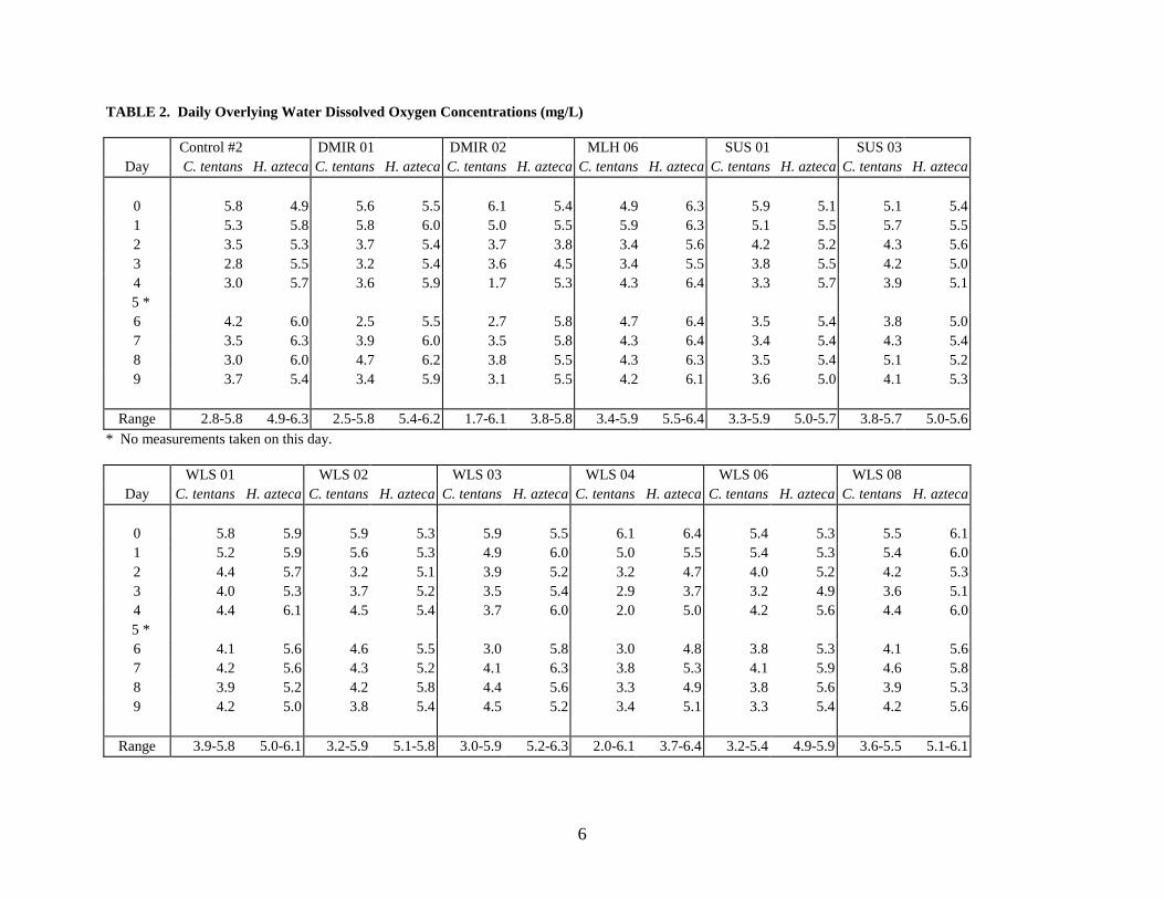
6

TABLE 2. Daily Overlying Water Dissolved Oxygen Concentrations (mg/L)

Control #2 DMIR 01 DMIR 02 MLH 06 SUS 01 SUS 03Day C. tentans H. azteca C. tentans H. azteca C. tentans H. azteca C. tentans H. azteca C. tentans H. azteca C. tentans H. azteca

0 5.8 4.9 5.6 5.5 6.1 5.4 4.9 6.3 5.9 5.1 5.1 5.41 5.3 5.8 5.8 6.0 5.0 5.5 5.9 6.3 5.1 5.5 5.7 5.52 3.5 5.3 3.7 5.4 3.7 3.8 3.4 5.6 4.2 5.2 4.3 5.63 2.8 5.5 3.2 5.4 3.6 4.5 3.4 5.5 3.8 5.5 4.2 5.04 3.0 5.7 3.6 5.9 1.7 5.3 4.3 6.4 3.3 5.7 3.9 5.1

5 *6 4.2 6.0 2.5 5.5 2.7 5.8 4.7 6.4 3.5 5.4 3.8 5.07 3.5 6.3 3.9 6.0 3.5 5.8 4.3 6.4 3.4 5.4 4.3 5.48 3.0 6.0 4.7 6.2 3.8 5.5 4.3 6.3 3.5 5.4 5.1 5.29 3.7 5.4 3.4 5.9 3.1 5.5 4.2 6.1 3.6 5.0 4.1 5.3

Range 2.8-5.8 4.9-6.3 2.5-5.8 5.4-6.2 1.7-6.1 3.8-5.8 3.4-5.9 5.5-6.4 3.3-5.9 5.0-5.7 3.8-5.7 5.0-5.6* No measurements taken on this day.

WLS 01 WLS 02 WLS 03 WLS 04 WLS 06 WLS 08Day C. tentans H. azteca C. tentans H. azteca C. tentans H. azteca C. tentans H. azteca C. tentans H. azteca C. tentans H. azteca

0 5.8 5.9 5.9 5.3 5.9 5.5 6.1 6.4 5.4 5.3 5.5 6.11 5.2 5.9 5.6 5.3 4.9 6.0 5.0 5.5 5.4 5.3 5.4 6.02 4.4 5.7 3.2 5.1 3.9 5.2 3.2 4.7 4.0 5.2 4.2 5.33 4.0 5.3 3.7 5.2 3.5 5.4 2.9 3.7 3.2 4.9 3.6 5.14 4.4 6.1 4.5 5.4 3.7 6.0 2.0 5.0 4.2 5.6 4.4 6.0

5 *6 4.1 5.6 4.6 5.5 3.0 5.8 3.0 4.8 3.8 5.3 4.1 5.67 4.2 5.6 4.3 5.2 4.1 6.3 3.8 5.3 4.1 5.9 4.6 5.88 3.9 5.2 4.2 5.8 4.4 5.6 3.3 4.9 3.8 5.6 3.9 5.39 4.2 5.0 3.8 5.4 4.5 5.2 3.4 5.1 3.3 5.4 4.2 5.6

Range 3.9-5.8 5.0-6.1 3.2-5.9 5.1-5.8 3.0-5.9 5.2-6.3 2.0-6.1 3.7-6.4 3.2-5.4 4.9-5.9 3.6-5.5 5.1-6.1

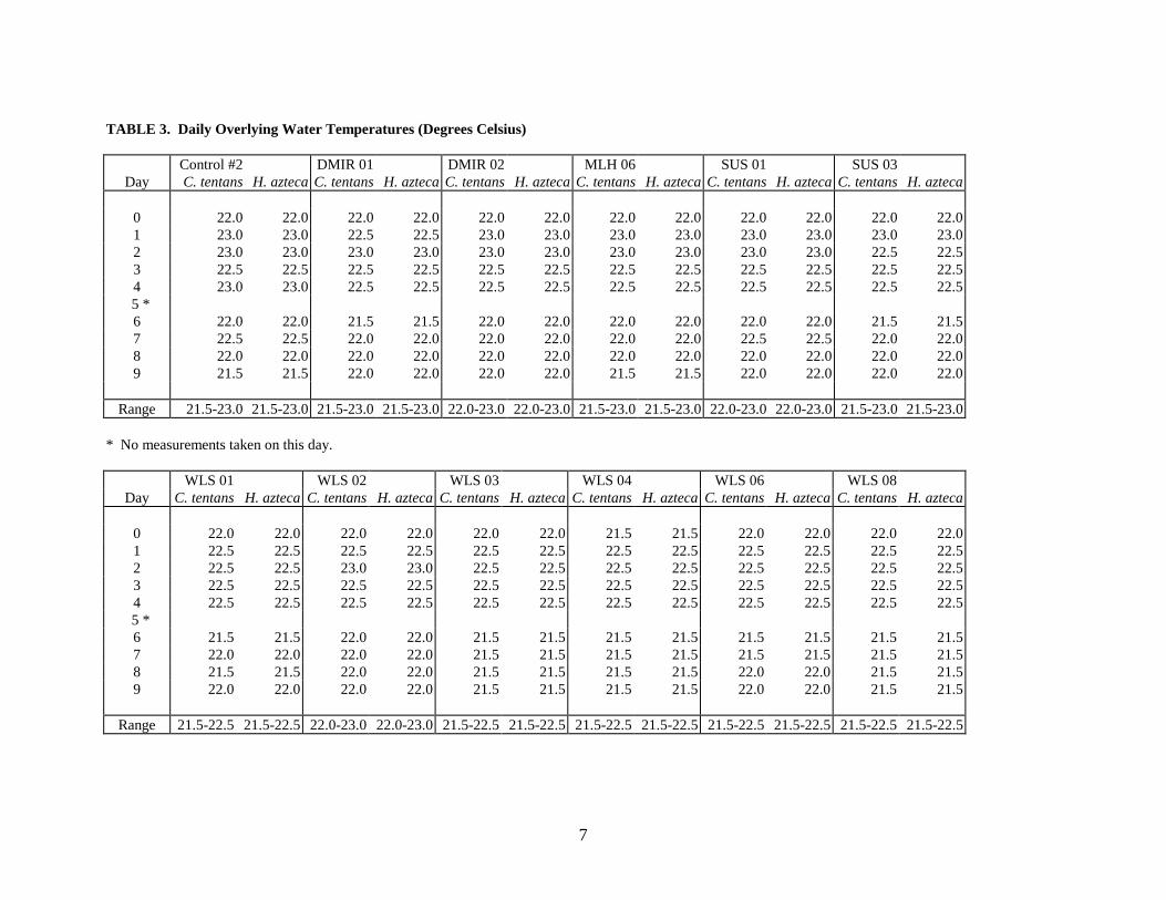
7

TABLE 3. Daily Overlying Water Temperatures (Degrees Celsius)

Control #2 DMIR 01 DMIR 02 MLH 06 SUS 01 SUS 03Day C. tentans H. azteca C. tentans H. azteca C. tentans H. azteca C. tentans H. azteca C. tentans H. azteca C. tentans H. azteca

0 22.0 22.0 22.0 22.0 22.0 22.0 22.0 22.0 22.0 22.0 22.0 22.01 23.0 23.0 22.5 22.5 23.0 23.0 23.0 23.0 23.0 23.0 23.0 23.02 23.0 23.0 23.0 23.0 23.0 23.0 23.0 23.0 23.0 23.0 22.5 22.53 22.5 22.5 22.5 22.5 22.5 22.5 22.5 22.5 22.5 22.5 22.5 22.54 23.0 23.0 22.5 22.5 22.5 22.5 22.5 22.5 22.5 22.5 22.5 22.5

5 *6 22.0 22.0 21.5 21.5 22.0 22.0 22.0 22.0 22.0 22.0 21.5 21.57 22.5 22.5 22.0 22.0 22.0 22.0 22.0 22.0 22.5 22.5 22.0 22.08 22.0 22.0 22.0 22.0 22.0 22.0 22.0 22.0 22.0 22.0 22.0 22.09 21.5 21.5 22.0 22.0 22.0 22.0 21.5 21.5 22.0 22.0 22.0 22.0

Range 21.5-23.0 21.5-23.0 21.5-23.0 21.5-23.0 22.0-23.0 22.0-23.0 21.5-23.0 21.5-23.0 22.0-23.0 22.0-23.0 21.5-23.0 21.5-23.0

* No measurements taken on this day.

WLS 01 WLS 02 WLS 03 WLS 04 WLS 06 WLS 08Day C. tentans H. azteca C. tentans H. azteca C. tentans H. azteca C. tentans H. azteca C. tentans H. azteca C. tentans H. azteca

0 22.0 22.0 22.0 22.0 22.0 22.0 21.5 21.5 22.0 22.0 22.0 22.01 22.5 22.5 22.5 22.5 22.5 22.5 22.5 22.5 22.5 22.5 22.5 22.52 22.5 22.5 23.0 23.0 22.5 22.5 22.5 22.5 22.5 22.5 22.5 22.53 22.5 22.5 22.5 22.5 22.5 22.5 22.5 22.5 22.5 22.5 22.5 22.54 22.5 22.5 22.5 22.5 22.5 22.5 22.5 22.5 22.5 22.5 22.5 22.5

5 *6 21.5 21.5 22.0 22.0 21.5 21.5 21.5 21.5 21.5 21.5 21.5 21.57 22.0 22.0 22.0 22.0 21.5 21.5 21.5 21.5 21.5 21.5 21.5 21.58 21.5 21.5 22.0 22.0 21.5 21.5 21.5 21.5 22.0 22.0 21.5 21.59 22.0 22.0 22.0 22.0 21.5 21.5 21.5 21.5 22.0 22.0 21.5 21.5

Range 21.5-22.5 21.5-22.5 22.0-23.0 22.0-23.0 21.5-22.5 21.5-22.5 21.5-22.5 21.5-22.5 21.5-22.5 21.5-22.5 21.5-22.5 21.5-22.5

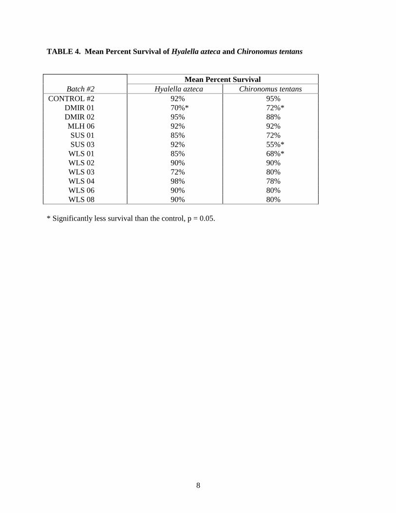
8

TABLE 4. Mean Percent Survival of Hyalella azteca and Chironomus tentans

Mean Percent SurvivalBatch #2 Hyalella azteca Chironomus tentans

CONTROL #2 92% 95%DMIR 01 70%* 72%*DMIR 02 95% 88%MLH 06 92% 92%SUS 01 85% 72%SUS 03 92% 55%*

WLS 01 85% 68%*WLS 02 90% 90%WLS 03 72% 80%WLS 04 98% 78%WLS 06 90% 80%WLS 08 90% 80%

* Significantly less survival than the control, p = 0.05.

APPENDIX A

Statistical Analyses

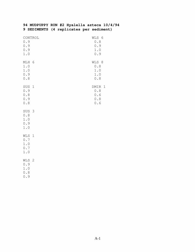
A-1

94 MUDPUPPY RUN #2 Hyalella azteca 10/4/949 SEDIMENTS (4 replicates per sediment)

CONTROL WLS 60.9 0.80.9 0.90.9 1.01.0 0.9

MLH 6 WLS 81.0 0.81.0 1.00.9 1.00.8 0.8

SUS 1 DMIR 10.9 0.80.8 0.60.9 0.80.8 0.6

SUS 30.81.00.91.0

WLS 10.71.00.71.0

WLS 20.91.00.80.9

A-2

TITLE: 94 MUDPUPPY RUN #2 Hyalella azteca 10/4/94FILE: 94MUD2X.DATTRANSFORM: ARC SINE(SQUARE ROOT(Y)) NUMBER OF GROUPS: 9-------------------------------------------------------------------

GRP IDENTIFICATION REP VALUE TRANS VALUE--- ---------------- ---- ------------- -------------1 CONTROL 1 0.9000 1.24901 CONTROL 2 0.9000 1.24901 CONTROL 3 0.9000 1.24901 CONTROL 4 1.0000 1.41202 MLH 6 1 1.0000 1.41202 MLH 6 2 1.0000 1.41202 MLH 6 3 0.9000 1.24902 MLH 6 4 0.8000 1.10713 SUS 1 1 0.9000 1.24903 SUS 1 2 0.8000 1.10713 SUS 1 3 0.9000 1.24903 SUS 1 4 0.8000 1.10714 SUS 3 1 0.8000 1.10714 SUS 3 2 1.0000 1.41204 SUS 3 3 0.9000 1.24904 SUS 3 4 1.0000 1.41205 WLS 1 1 0.7000 0.99125 WLS 1 2 1.0000 1.41205 WLS 1 3 0.7000 0.99125 WLS 1 4 1.0000 1.41206 WLS 2 1 0.9000 1.24906 WLS 2 2 1.0000 1.41206 WLS 2 3 0.8000 1.10716 WLS 2 4 0.9000 1.24907 WLS 6 1 0.8000 1.10717 WLS 6 2 0.9000 1.24907 WLS 6 3 1.0000 1.41207 WLS 6 4 0.9000 1.24908 WLS 8 1 0.8000 1.10718 WLS 8 2 1.0000 1.41208 WLS 8 3 1.0000 1.41208 WLS 8 4 0.8000 1.10719 DMIR 1 1 0.8000 1.10719 DMIR 1 2 0.6000 0.88619 DMIR 1 3 0.8000 1.10719 DMIR 1 4 0.6000 0.8861-------------------------------------------------------------------

A-3

94 MUDPUPPY RUN #2C Hyalella azteca 10/4/94File: 94MUD2X.DAT Transform: ARC SINE(SQUARE ROOT(Y))

SUMMARY STATISTICS ON TRANSFORMED DATA TABLE 1 of 2-----------------------------------------------------------------------

GRP IDENTIFICATION N MIN MAX MEAN--- ---------------- ---- ---------- ---------- ----------1 CONTROL 4 1.249 1.412 1.2902 MLH 6 4 1.107 1.412 1.2953 SUS 1 4 1.107 1.249 1.1784 SUS 3 4 1.107 1.412 1.2955 WLS 1 4 0.991 1.412 1.2026 WLS 2 4 1.107 1.412 1.2547 WLS 6 4 1.107 1.412 1.2548 WLS 8 4 1.107 1.412 1.2609 DMIR 1 4 0.886 1.107 0.997------------------------------------------------------------------------

94 MUDPUPPY RUN #2C Hyalella azteca 10/4/94File: 94MUD2X.DAT Transform: ARC SINE(SQUARE ROOT(Y))

SUMMARY STATISTICS ON TRANSFORMED DATA TABLE 2 of 2-----------------------------------------------------------------------

GRP IDENTIFICATION VARIANCE SD SEM C.V. %--- ---------------- -------------- ---------- ---------- ----------1 CONTROL 0.007 0.081 0.041 6.322 MLH 6 0.022 0.147 0.073 11.353 SUS 1 0.007 0.082 0.041 6.954 SUS 3 0.022 0.147 0.073 11.355 WLS 1 0.059 0.243 0.121 20.226 WLS 2 0.016 0.125 0.062 9.937 WLS 6 0.016 0.125 0.062 9.938 WLS 8 0.031 0.176 0.088 13.979 DMIR 1 0.016 0.128 0.064 12.81------------------------------------------------------------------------

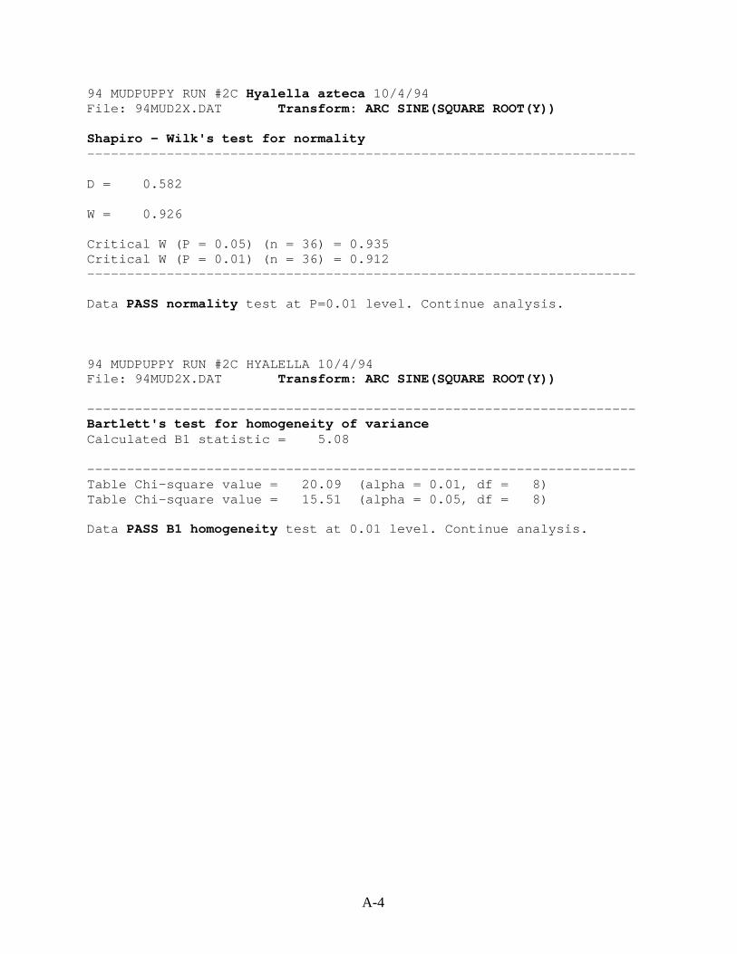
A-4

94 MUDPUPPY RUN #2C Hyalella azteca 10/4/94File: 94MUD2X.DAT Transform: ARC SINE(SQUARE ROOT(Y))

Shapiro - Wilk's test for normality---------------------------------------------------------------------

D = 0.582

W = 0.926

Critical W (P = 0.05) (n = 36) = 0.935Critical W (P = 0.01) (n = 36) = 0.912---------------------------------------------------------------------

Data PASS normality test at P=0.01 level. Continue analysis.

94 MUDPUPPY RUN #2C HYALELLA 10/4/94File: 94MUD2X.DAT Transform: ARC SINE(SQUARE ROOT(Y))

---------------------------------------------------------------------Bartlett's test for homogeneity of varianceCalculated B1 statistic = 5.08

---------------------------------------------------------------------Table Chi-square value = 20.09 (alpha = 0.01, df = 8)Table Chi-square value = 15.51 (alpha = 0.05, df = 8)

Data PASS B1 homogeneity test at 0.01 level. Continue analysis.

A-5

94 MUDPUPPY RUN #2C Hyalella azteca 10/4/94File: 94MUD2X.DAT Transform: ARC SINE(SQUARE ROOT(Y))

ANOVA TABLE------------------------------------------------------------------------------

SOURCE DF SS MS F------------------------------------------------------------------------------Between 8 0.287 0.036 1.667

Within (Error) 27 0.582 0.022------------------------------------------------------------------------------Total 35 0.869------------------------------------------------------------------------------

Critical F value = 2.31 (0.05,8,27)Since F < Critical F FAIL TO REJECT Ho: All equal

94 MUDPUPPY RUN #2 Hyalella azteca 10/4/94File: 94MUD2X.DAT Transform: ARC SINE(SQUARE ROOT(Y))

DUNNETT'S TEST - TABLE 1 OF 2 Ho:Control<Treatment----------------------------------------------------------------------------

TRANSFORMED MEAN CALCULATED INGROUP IDENTIFICATION MEAN ORIGINAL UNITS T STAT SIG----- -------------------- ----------- ------------------ ------ ---

1 CONTROL 1.290 0.9252 MLH 6 1.295 0.925 -0.0513 SUS 1 1.178 0.850 1.0764 SUS 3 1.295 0.925 -0.0515 WLS 1 1.202 0.850 0.8506 WLS 2 1.254 0.900 0.3427 WLS 6 1.254 0.900 0.3428 WLS 8 1.260 0.900 0.2919 DMIR 1 0.997 0.700 2.825 *

----------------------------------------------------------------------------Dunnett table value = 2.53 (1 Tailed Value, P=0.05, df=24,8)

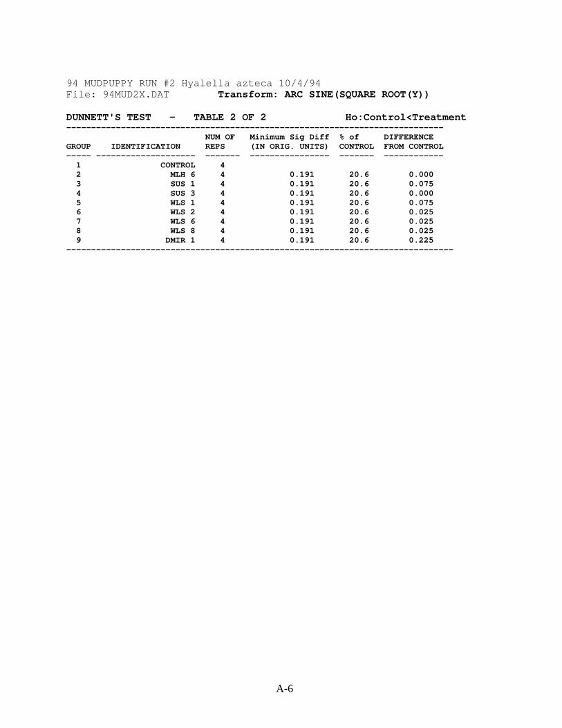
A-6

94 MUDPUPPY RUN #2 Hyalella azteca 10/4/94File: 94MUD2X.DAT Transform: ARC SINE(SQUARE ROOT(Y))

DUNNETT'S TEST - TABLE 2 OF 2 Ho:Control<Treatment----------------------------------------------------------------------------

NUM OF Minimum Sig Diff % of DIFFERENCEGROUP IDENTIFICATION REPS (IN ORIG. UNITS) CONTROL FROM CONTROL----- -------------------- ------- ---------------- ------- ------------

1 CONTROL 42 MLH 6 4 0.191 20.6 0.0003 SUS 1 4 0.191 20.6 0.0754 SUS 3 4 0.191 20.6 0.0005 WLS 1 4 0.191 20.6 0.0756 WLS 2 4 0.191 20.6 0.0257 WLS 6 4 0.191 20.6 0.0258 WLS 8 4 0.191 20.6 0.0259 DMIR 1 4 0.191 20.6 0.225

------------------------------------------------------------------------------

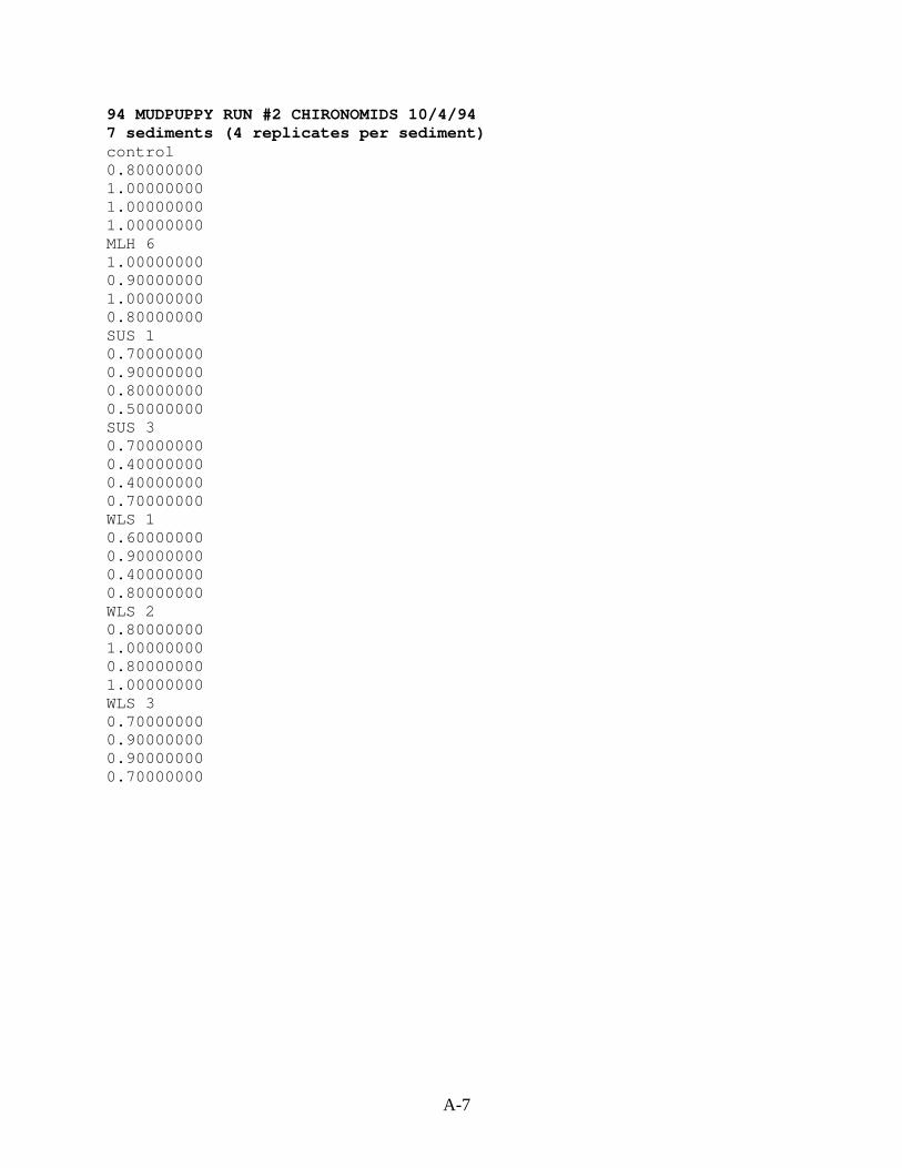
A-7

94 MUDPUPPY RUN #2 CHIRONOMIDS 10/4/947 sediments (4 replicates per sediment)control0.800000001.000000001.000000001.00000000MLH 61.000000000.900000001.000000000.80000000SUS 10.700000000.900000000.800000000.50000000SUS 30.700000000.400000000.400000000.70000000WLS 10.600000000.900000000.400000000.80000000WLS 20.800000001.000000000.800000001.00000000WLS 30.700000000.900000000.900000000.70000000

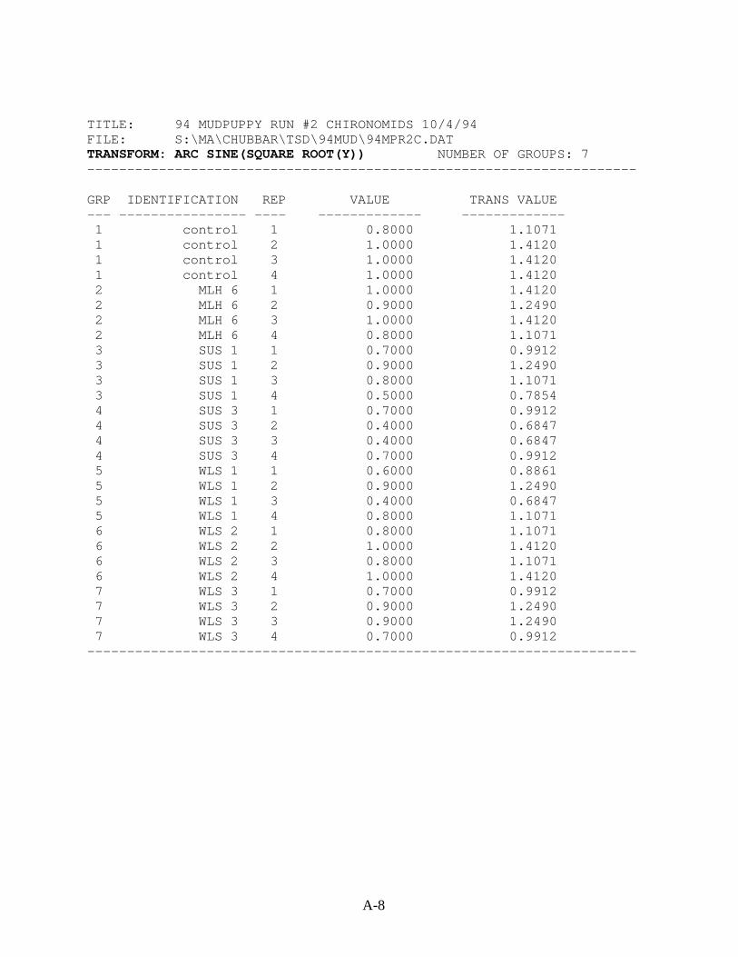
A-8

TITLE: 94 MUDPUPPY RUN #2 CHIRONOMIDS 10/4/94FILE: S:\MA\CHUBBAR\TSD\94MUD\94MPR2C.DATTRANSFORM: ARC SINE(SQUARE ROOT(Y)) NUMBER OF GROUPS: 7---------------------------------------------------------------------

GRP IDENTIFICATION REP VALUE TRANS VALUE--- ---------------- ---- ------------- -------------1 control 1 0.8000 1.10711 control 2 1.0000 1.41201 control 3 1.0000 1.41201 control 4 1.0000 1.41202 MLH 6 1 1.0000 1.41202 MLH 6 2 0.9000 1.24902 MLH 6 3 1.0000 1.41202 MLH 6 4 0.8000 1.10713 SUS 1 1 0.7000 0.99123 SUS 1 2 0.9000 1.24903 SUS 1 3 0.8000 1.10713 SUS 1 4 0.5000 0.78544 SUS 3 1 0.7000 0.99124 SUS 3 2 0.4000 0.68474 SUS 3 3 0.4000 0.68474 SUS 3 4 0.7000 0.99125 WLS 1 1 0.6000 0.88615 WLS 1 2 0.9000 1.24905 WLS 1 3 0.4000 0.68475 WLS 1 4 0.8000 1.10716 WLS 2 1 0.8000 1.10716 WLS 2 2 1.0000 1.41206 WLS 2 3 0.8000 1.10716 WLS 2 4 1.0000 1.41207 WLS 3 1 0.7000 0.99127 WLS 3 2 0.9000 1.24907 WLS 3 3 0.9000 1.24907 WLS 3 4 0.7000 0.9912---------------------------------------------------------------------

A-9

94 MUDPUPPY RUN #2 CHIRONOMIDS 10/4/94File: S:\MA\CHUBBAR\TSD\94MUD\94MPR2C.DAT Transform: ARCSINE(SQUARE ROOT(Y))

SUMMARY STATISTICS ON TRANSFORMED DATA TABLE 1 of 2-----------------------------------------------------------------------

GRP IDENTIFICATION N MIN MAX MEAN--- ---------------- ---- ---------- ---------- ----------1 control 4 1.107 1.412 1.3362 MLH 6 4 1.107 1.412 1.2953 SUS 1 4 0.785 1.249 1.0334 SUS 3 4 0.685 0.991 0.8385 WLS 1 4 0.685 1.249 0.9826 WLS 2 4 1.107 1.412 1.2607 WLS 3 4 0.991 1.249 1.120-----------------------------------------------------------------------

94 MUDPUPPY RUN#2 CHIRONOMIDS 10/4/94File: S:\MA\CHUBBAR\TSD\94MUD\94MPR2C.DATTransform: ARC SINE(SQUARE ROOT(Y))

SUMMARY STATISTICS ON TRANSFORMED DATA TABLE 2 of 2------------------------------------------------------------------------

GRP IDENTIFICATION VARIANCE SD SEM C.V. %--- ---------------- -------------- ---------- ---------- ----------1 control 0.023 0.152 0.076 11.412 MLH 6 0.022 0.147 0.073 11.353 SUS 1 0.038 0.196 0.098 18.974 SUS 3 0.031 0.177 0.088 21.115 WLS 1 0.062 0.248 0.124 25.266 WLS 2 0.031 0.176 0.088 13.977 WLS 3 0.022 0.149 0.074 13.29------------------------------------------------------------------------

A-10

94 MUDPUPPY RUN #2 CHIRONOMIDS 10/4/94File: S:\MA\CHUBBAR\TSD\94MUD\94MPR2C.DATTransform: ARC SINE(SQUARE ROOT(Y))

Shapiro - Wilk's test for normality---------------------------------------------------------------------

D = 0.688

W = 0.916

Critical W (P = 0.05) (n = 28) = 0.924Critical W (P = 0.01) (n = 28) = 0.896---------------------------------------------------------------------

Data PASS normality test at P=0.01 level. Continue analysis.

94 MUDPUPPY RUN #2 CHIRONOMIDS 10/4/94File: S:\MA\CHUBBAR\TSD\94MUD\94MPR2C.DATTransform: ARC SINE(SQUARE ROOT(Y))

---------------------------------------------------------------------Bartlett's test for homogeneity of varianceCalculated B1 statistic = 1.22

---------------------------------------------------------------------Table Chi-square value = 16.81 (alpha = 0.01, df = 6)Table Chi-square value = 12.59 (alpha = 0.05, df = 6)

Data PASS B1 homogeneity test at 0.01 level. Continue analysis.

A-11

94 MUDPUPPY RUN#2 CHIRONOMIDS 10/4/94File: S:\MA\CHUBBAR\TSD\94MUD\94MPR2C.DATTransform: ARC SINE(SQUARE ROOT(Y))

ANOVA TABLE------------------------------------------------------------------------------

SOURCE DF SS MS F------------------------------------------------------------------------------Between 6 0.811 0.135 4.130

Within (Error) 21 0.688 0.033------------------------------------------------------------------------------Total 27 1.499------------------------------------------------------------------------------

Critical F value = 2.57 (0.05,6,21)Since F > Critical F REJECT Ho: All equal

94 MUDPUPPY RUN #2 CHIRONOMIDS 10/4/94File: S:\MA\CHUBBAR\TSD\94MUD\94MPR2C.DATTransform: ARC SINE(SQUARE ROOT(Y))

DUNNETT'S TEST - TABLE 1 OF 2 Ho:Control<Treatment----------------------------------------------------------------------------

TRANSFORMED MEAN CALCULATED INGROUP IDENTIFICATION MEAN ORIGINAL UNITS T STAT SIG----- -------------------- ----------- ------------------ ------ ---

1 control 1.336 0.9502 MLH 6 1.295 0.925 0.3183 SUS 1 1.033 0.725 2.3654 SUS 3 0.838 0.550 3.891 *5 WLS 1 0.982 0.675 2.767 *6 WLS 2 1.260 0.900 0.5967 WLS 3 1.120 0.800 1.686

----------------------------------------------------------------------------Dunnett table value = 2.46 (1 Tailed Value, P=0.05, df=20,6)

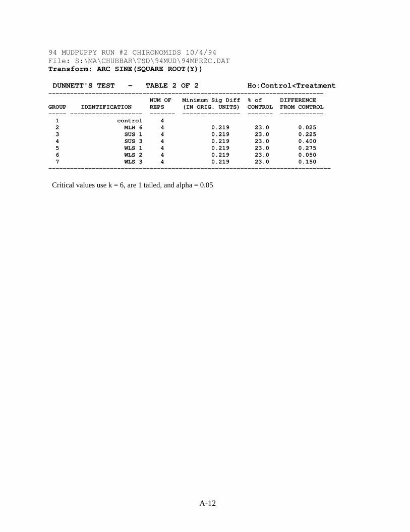
A-12

94 MUDPUPPY RUN #2 CHIRONOMIDS 10/4/94File: S:\MA\CHUBBAR\TSD\94MUD\94MPR2C.DATTransform: ARC SINE(SQUARE ROOT(Y))

DUNNETT'S TEST - TABLE 2 OF 2 Ho:Control<Treatment----------------------------------------------------------------------------

NUM OF Minimum Sig Diff % of DIFFERENCEGROUP IDENTIFICATION REPS (IN ORIG. UNITS) CONTROL FROM CONTROL----- -------------------- ------- ---------------- ------- ------------

1 control 42 MLH 6 4 0.219 23.0 0.0253 SUS 1 4 0.219 23.0 0.2254 SUS 3 4 0.219 23.0 0.4005 WLS 1 4 0.219 23.0 0.2756 WLS 2 4 0.219 23.0 0.0507 WLS 3 4 0.219 23.0 0.150

------------------------------------------------------------------------------

Critical values use k = 6, are 1 tailed, and alpha = 0.05

A-13

94 MUDPUPPY RUN #2 ADD'L C.tentans6 sediments (4 replicates per sediments)444444CONTROL0.81.01.01.0

WLS 40.80.80.90.6

WLS 61.00.80.60.8

WLS 80.90.80.90.6

DMIR 10.70.70.80.7

DMIR 20.90.90.80.9

A-14

TITLE: 94 MUDPUPPY RUN#2 ADD'L C.TENTANSFILE: 94MPR2CD.DATTRANSFORM: ARC SINE(SQUARE ROOT(Y)) NUMBER OF GROUPS: 6---------------------------------------------------------------------

GRP IDENTIFICATION REP VALUE TRANS VALUE--- ---------------- ---- ------------- -------------1 CONTROL 1 0.8000 1.10711 CONTROL 2 1.0000 1.41201 CONTROL 3 1.0000 1.41201 CONTROL 4 1.0000 1.41202 WLS 4 1 0.8000 1.10712 WLS 4 2 0.8000 1.10712 WLS 4 3 0.9000 1.24902 WLS 4 4 0.6000 0.88613 WLS 6 1 1.0000 1.41203 WLS 6 2 0.8000 1.10713 WLS 6 3 0.6000 0.88613 WLS 6 4 0.8000 1.10714 WLS 8 1 0.9000 1.24904 WLS 8 2 0.8000 1.10714 WLS 8 3 0.9000 1.24904 WLS 8 4 0.6000 0.88615 DMIR 1 1 0.7000 0.99125 DMIR 1 2 0.7000 0.99125 DMIR 1 3 0.8000 1.10715 DMIR 1 4 0.7000 0.99126 DMIR 2 1 0.9000 1.24906 DMIR 2 2 0.9000 1.24906 DMIR 2 3 0.8000 1.10716 DMIR 2 4 0.9000 1.2490---------------------------------------------------------------------

A-15

94 MUDPUPPY RUN#2 ADD'L C.TENTANSFile: 94MPR2CD.DAT Transform: ARC SINE(SQUARE ROOT(Y))

SUMMARY STATISTICS ON TRANSFORMED DATA TABLE 1 of 2----------------------------------------------------------------------

GRP IDENTIFICATION N MIN MAX MEAN--- ---------------- ---- ---------- ---------- ----------1 CONTROL 4 1.107 1.412 1.3362 WLS 4 4 0.886 1.249 1.0873 WLS 6 4 0.886 1.412 1.1284 WLS 8 4 0.886 1.249 1.1235 DMIR 1 4 0.991 1.107 1.0206 DMIR 2 4 1.107 1.249 1.214----------------------------------------------------------------------

94 MUDPUPPY RUN#2 ADD'L C.TENTANSFile: 94MPR2CD.DAT Transform: ARC SINE(SQUARE ROOT(Y))

SUMMARY STATISTICS ON TRANSFORMED DATA TABLE 2 of 2------------------------------------------------------------------------

GRP IDENTIFICATION VARIANCE SD SEM C.V. %--- ---------------- -------------- ---------- ---------- ----------1 CONTROL 0.023 0.152 0.076 11.412 WLS 4 0.022 0.150 0.075 13.793 WLS 6 0.047 0.216 0.108 19.154 WLS 8 0.029 0.171 0.086 15.275 DMIR 1 0.003 0.058 0.029 5.696 DMIR 2 0.005 0.071 0.035 5.85------------------------------------------------------------------------

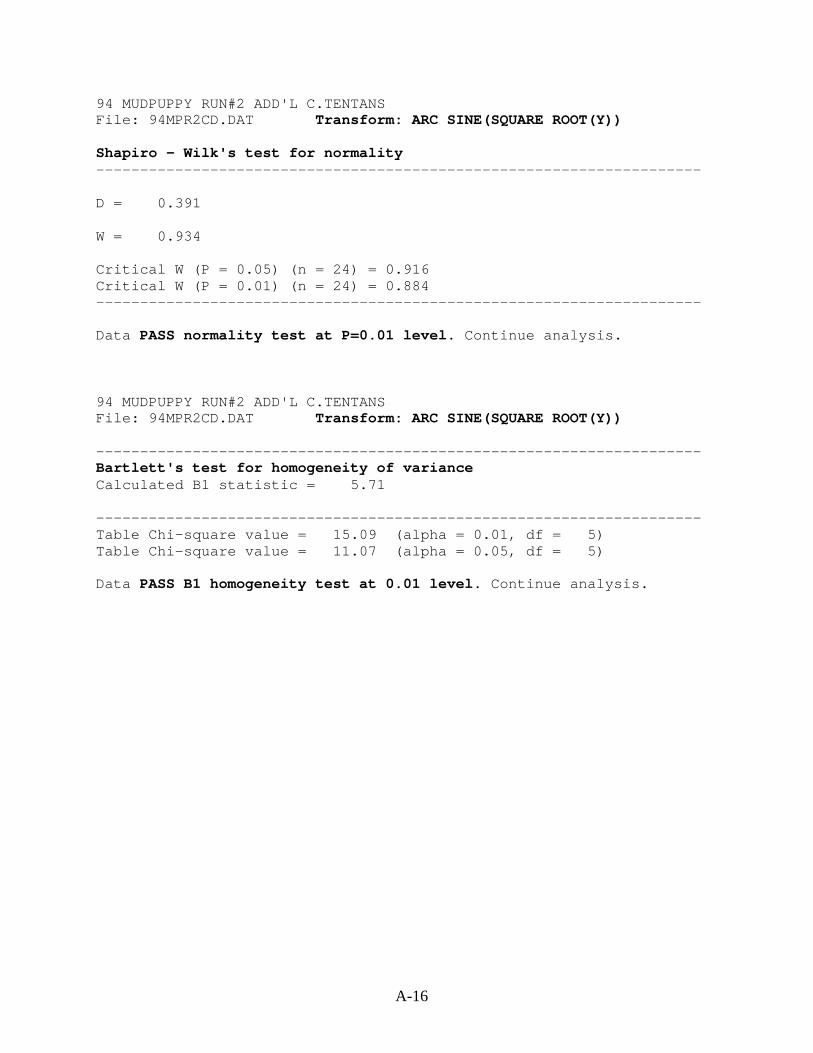
A-16

94 MUDPUPPY RUN#2 ADD'L C.TENTANSFile: 94MPR2CD.DAT Transform: ARC SINE(SQUARE ROOT(Y))

Shapiro - Wilk's test for normality---------------------------------------------------------------------

D = 0.391

W = 0.934

Critical W (P = 0.05) (n = 24) = 0.916Critical W (P = 0.01) (n = 24) = 0.884---------------------------------------------------------------------

Data PASS normality test at P=0.01 level. Continue analysis.

94 MUDPUPPY RUN#2 ADD'L C.TENTANSFile: 94MPR2CD.DAT Transform: ARC SINE(SQUARE ROOT(Y))

---------------------------------------------------------------------Bartlett's test for homogeneity of varianceCalculated B1 statistic = 5.71

---------------------------------------------------------------------Table Chi-square value = 15.09 (alpha = 0.01, df = 5)Table Chi-square value = 11.07 (alpha = 0.05, df = 5)

Data PASS B1 homogeneity test at 0.01 level. Continue analysis.

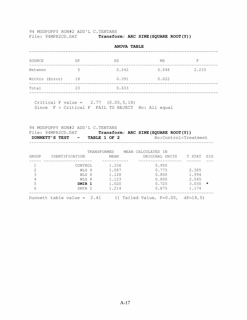
A-17

94 MUDPUPPY RUN#2 ADD'L C.TENTANSFile: 94MPR2CD.DAT Transform: ARC SINE(SQUARE ROOT(Y))

ANOVA TABLE------------------------------------------------------------------------------

SOURCE DF SS MS F------------------------------------------------------------------------------Between 5 0.242 0.048 2.233

Within (Error) 18 0.391 0.022------------------------------------------------------------------------------Total 23 0.633------------------------------------------------------------------------------

Critical F value = 2.77 (0.05,5,18)Since F < Critical F FAIL TO REJECT Ho: All equal

94 MUDPUPPY RUN#2 ADD'L C.TENTANSFile: 94MPR2CD.DAT Transform: ARC SINE(SQUARE ROOT(Y))DUNNETT'S TEST - TABLE 1 OF 2 Ho:Control<Treatment

----------------------------------------------------------------------------

TRANSFORMED MEAN CALCULATED INGROUP IDENTIFICATION MEAN ORIGINAL UNITS T STAT SIG----- -------------------- ----------- ------------------ ------ ---

1 CONTROL 1.336 0.9502 WLS 4 1.087 0.775 2.3853 WLS 6 1.128 0.800 1.9944 WLS 8 1.123 0.800 2.0455 DMIR 1 1.020 0.725 3.030 *6 DMIR 2 1.214 0.875 1.174

----------------------------------------------------------------------------Dunnett table value = 2.41 (1 Tailed Value, P=0.05, df=18,5)

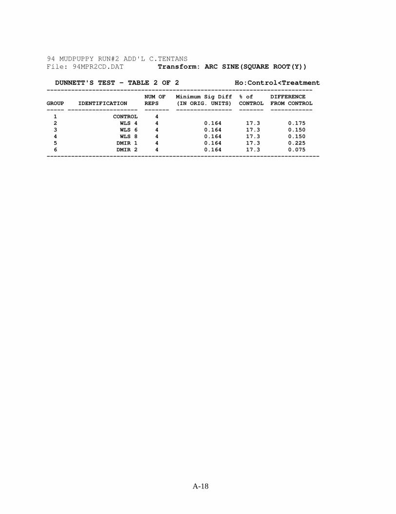
A-18

94 MUDPUPPY RUN#2 ADD'L C.TENTANSFile: 94MPR2CD.DAT Transform: ARC SINE(SQUARE ROOT(Y))

DUNNETT'S TEST - TABLE 2 OF 2 Ho:Control<Treatment----------------------------------------------------------------------------

NUM OF Minimum Sig Diff % of DIFFERENCEGROUP IDENTIFICATION REPS (IN ORIG. UNITS) CONTROL FROM CONTROL----- -------------------- ------- ---------------- ------- ------------

1 CONTROL 42 WLS 4 4 0.164 17.3 0.1753 WLS 6 4 0.164 17.3 0.1504 WLS 8 4 0.164 17.3 0.1505 DMIR 1 4 0.164 17.3 0.2256 DMIR 2 4 0.164 17.3 0.075

------------------------------------------------------------------------------

ACUTE TOXICITY TESTSWITH

HYALELLA AZTECA AND CHIRONOMUS TENTANSON SEDIMENTS FROM THE DULUTH/SUPERIOR HARBOR:

1994 Sampling Results - Batch # 3

Conducted by

Minnesota Pollution Control AgencyMonitoring and Assessment Section

520 Lafayette RoadSt. Paul, Minnesota 55155-4194

April 1997

ii

TABLE OF CONTENTS

INTRODUCTION . . . . . . . . . . . . . . . . . . . . . . . . . . . . . . . . . . . . . . . . . . . . . . . . . . . . . . . . . . . . 1

SAMPLE COLLECTION AND HANDLING . . . . . . . . . . . . . . . . . . . . . . . . . . . . . . . . . . . . . . 1

METHODS .. . . . . . . . . . . . . . . . . . . . . . . . . . . . . . . . . . . . . . . . . . . . . . . . . . . . . . . . . . . . . . . . 1

RESULTS . . . . . . . . . . . . . . . . . . . . . . . . . . . . . . . . . . . . . . . . . . . . . . . . . . . . . . . . . . . . . . . . . . 3

SUMMARY . . . . . . . . . . . . . . . . . . . . . . . . . . . . . . . . . . . . . . . . . . . . . . . . . . . . . . . . . . . . . . . . 4

REFERENCES . . . . . . . . . . . . . . . . . . . . . . . . . . . . . . . . . . . . . . . . . . . . . . . . . . . . . . . . . . . . . . . 5

APPENDIX A - Statistical Analyses

iii

LIST OF TABLES

TABLE 1. Daily Overlying Water pH Measurements ..................................................................6

TABLE 2. Daily Overlying Water Dissolved Oxygen Concentrations (mg/L).............................7

TABLE 3. Daily Overlying Water Temperatures (Degrees Celsius)........................................... 8

TABLE 4. Mean Percent Survival of Hyalella azteca and Chironomus tentans .......................... 9

1

INTRODUCTION

As part of a sediment assessment of hotspot areas in the Duluth/Superior Harbor, sedimenttoxicity tests were conducted to assess acute (survival) and chronic (growth) toxicity to benthicinvertebrates. Acute effects were measured in separate 10-day toxicity tests to Hyalella azteca(H. azteca) and Chironomus tentans (C. tentans). Growth was measured at the end of theC. tentans test to assess chronic effects. Survival and growth endpoints were compared toorganisms similarly exposed to a reference control sediment collected from West Bearskin Lake(Cook County, MN).

A total of 44 sediment samples were collected for toxicity testing. This report presents theresults of eleven of these sediment samples.

SAMPLE COLLECTION AND HANDLING

During September 22-30, 1994, Minnesota Pollution Control Agency (MPCA) staff collected theeleven sediments referred to in this report. The composited samples were collected from theharbor using a gravity corer. The samples were stored at 4°C at the Duluth MPCA office untilthey were transported to the MPCA Toxicology Laboratory in St. Paul, MN.

METHODS

Eleven sediment samples and a control sediment were subjected to the 10-day sediment toxicitytest using the procedures described in U.S. EPA (1994). The test organisms (H. azteca andC. tentans) were exposed to sediment samples in a portable, mini-flow system described inBenoit et al. (1993) and U.S. EPA (1994). The test apparatus consists of 300 mL, glass-beakertest chambers held in a glass box supplied with water from an acrylic plastic headbox. Thebeakers have two, 1.5 cm holes covered with stainless steel mesh, to allow for water exchangewhile containing the test organisms. The headbox has a pipette tip drain calibrated to deliverwater at an average rate of 32.5 mL/min. The glass box is fitted with a self-starting siphon toprovide exchange of overlying water.

The H. azteca used for this test were 1 to 3 mm long, and the C. tentans were approximately 14days old. These organisms were supplied by Environmental Consulting and Testing in Superior,WI. On the test set up day, MPCA personnel picked up the organisms from the supplier andtransported them to the MPCA Toxicology Laboratory.

2

On October 18, 1994, eleven samples (HOB 07, HOB 08, MNS 01, MNS 03, STP 01, STP 04,SUS 05, WLS 12, WLS 13, WLS 14, and WLS 16) and the control sediment were separatelyhomogenized by hand, and 100 mL of each sediment was placed in a test beaker (Batch #3).Each sediment test was set up with four replicates of H. azteca and four replicates of C. tentans.Approximately 100 mL of aerated, artesian well water was added to the beakers, and thesediments were allowed to settle for approximately two hours before the organisms were added.For the C. tentans test, ten organisms were placed in each of four beakers in a random fashion.Due to an insufficient number of H. azteca from the supplier, the four beakers for each sedimentsample were seeded as follows: seven organisms (Control #3, HOB 07, HOB 08, MNS 01,MNS 03, STP 04, replicates A and D of WLS 12, WLS 13, WLS 14, WLS 16), six organisms(STP 01, SUS 05, replicate B of WLS 12), and five organisms for replicate C of WLS 12.

The organisms were exposed to 16 hours of light and eight hours of darkness for the duration ofthe ten-day test. Each day, two liters of aerated water from the artesian well at Stroh Brewery inSt. Paul, MN were exchanged in each test chamber. On weekdays, 1-L was exchanged in themorning and 1-L in the afternoon. On weekends, the two liters were passed through thechambers all at once. Water quality measurements (i.e., pH, temperature, and dissolved oxygen)of the overlying water were taken in one beaker of each of the quadruplicate sets of each of thesediments. The results, along with daily observations involving the physical appearance of thesediments and organisms, were recorded in a laboratory notebook. This notebook is retained onfile at the MPCA.

The test was terminated on October 28, 1994. The sediments were sieved through 40 meshscreens, and the sieved material was sorted for organisms. The organisms found were counted,and the number of alive and dead organisms were recorded. Organisms not found were recordedas missing and presumed dead. The C. tentans that survived were placed in aluminum weighingdishes, dried at approximately 100°C for at least four hours, desiccated to room temperature, andweighed.

Growth (weight) of the C. tentans and survival of both organisms were used as the endpoints forthese tests. The survival data were analyzed using TOXSTAT (Gulley and WEST, Inc., 1994), astatistical software package obtained from the University of Wyoming. However, due to aquality assurance problem, the growth data were not analyzed.

A 96-hour, reference toxicant test with H. azteca in sodium chloride (NaCl) was run inconjunction with these toxicity tests to determine the acceptability of the H. azteca used. Fourconcentrations of NaCl solution (i.e., 10, 5, 2.5, and 1.25 g/L) and a control (aerated, artesianwell water) were used in this test. Due to a shortage of test organisms, only two replicates ofthree organisms each were set up per concentration.

3

RESULTS

Water Quality

Measurements of pH, dissolved oxygen, and temperature in the overlying water of the testbeakers were made daily. These measurements are summarized below and in Tables 1, 2, and 3,respectively.

The range of pH values in the beakers containing H. azteca was 7.6 to 8.3 (Table 1). The waterin the C. tentans beakers had a pH range of 7.7 to 8.4 (Table 1). The pH fluctuations duringthese tests were acceptable since they did not vary more than 50% within each treatment (U.S.EPA, 1994).

The dissolved oxygen concentration ranged from 2.5 to 6.6 mg/L in the H. azteca beakers andfrom 2.0 to 6.9 mg/L in the C. tentans beakers (Table 2). On days five, six, seven, eight, andnine, the dissolved oxygen concentrations in the MNS 03 sediment beakers containing bothC. tentans and H. azteca were less than 40% saturated. On days six, seven, and nine, thedissolved oxygen concentration in the MNS 01 beakers containing C. tentans were less than 40%saturated. The acceptable test range for dissolved oxygen is greater than 40% saturation (U.S.EPA, 1994). The organisms continued to be fed throughout the test.

The range of temperature values in the beakers containing H. azteca and C. tentans were both20.5° to 23.0°C (Table 3). The recommended temperature range for these tests is 23 ± 1°C(U.S. EPA, 1994).

Test Endpoints

Survival Data

The mean percent survival of the test organisms is summarized below and in Table 4.

The mean percent survival of H. azteca in the control was 89% with a range of 86% to 100%.The survival of this control was greater than 80%, and the test passed. For the control sedimentcontaining C. tentans, percent survival ranged from 30% to 80% with a mean of 52%. Survivalfor this control was less than 70% and, therefore, unacceptable. The C. tentans test failed for thebatch of sediments included in this test.

Mean percent survival of H. azteca in the test sediments ranged from 79% in the STP 01sediment to 100% in the HOB 08 and MNS 03 sediments. Two H. azteca sediment testsappeared to be mis-seeded. For WLS 16, it appears that replicate C was not seeded and replicateB was double seeded with 14 organisms. A weighted average was used to determine the meanpercent survival of the three replicates which had been seeded (i.e., 93%). For WLS 12, an extraorganism was found in two of the replicates; it was assumed that an error had been made inrecording the initial number of organisms. A mean percent survival of 96% was calculated forWLS 12.

4

Mean percent survival of C. tentans in the test sediments ranged from 28% in the HOB 08 andMNS 01 samples to 65% in the STP 04 sample.

C. Tentans Growth Data

Although the dried C. tentans were weighed, the balance on which they were weighed was notcalibrated with standard weights. Therefore, the data are suspect since the internal calibration ofthe balance may have drifted with time. Thus, no conclusions can be made regarding chronictoxicity (growth).

Data Analysis

A one-tailed Steel’s Many-one Rank test was used to test the alternative hypothesis that samplesurvival of H. azteca was less than control survival. Thus, it was not necessary to include theH. azteca mean percent survival data for samples which exceeded the control survival of 89%.The survival data for the control, MNS 01, and STP 01 were transformed using an arc sine-square root transformation prior to statistical analysis. Neither MNS 01 or STP 01 were toxic toH. azteca when compared to the control sediment (∝ = 0.05).

Reference Toxicant Test with Hyalella azteca in Sodium Chloride Solution

The pH of the overlying water in the reference toxicant test ranged from 8.0 to 8.4. Thedissolved oxygen ranged from 7.5 to 7.9 mg/L, and the temperature of the overlying water rangedfrom 21.0°C to 23.0°C.

There were not enough H. azteca to run the standard reference toxicant test; therefore, a test withtwo replicates per concentration containing three organisms each was run. The test met qualityassurance requirements for control survival (i.e., ≥ 90%) indicating that the H. azteca used in thistest were healthy. The LC50 value for this test was 2.29 g/L NaCl as determined by the TrimmedSpearman-Karber method. A control chart will be developed for this test once five data pointsare obtained. The LC50 value determined from this test will be flagged since an insufficientnumber of organisms and replicates were run for this test.

SUMMARY

Survival of H. azteca in the control sediments was acceptable (i.e., greater than 80%) and none ofthe test sediments resulted in significantly lower survival of H. azteca when compared to thecontrol survival (∝ = 0.05).

Control survival in the C. tentans test was unacceptable; therefore, the test failed. As a result, noconclusions may be drawn as to the toxicity of these sediments to C. tentans.

5

REFERENCES

Benoit, D.A., G. Phipps, and G.T. Ankley. 1993. A sediment testing intermittent renewal system for the automated renewal of overlying water in toxicity tests with contaminated sediments. Water Research 27:1403-1412.

Gulley, D.D. and WEST, Inc. 1994. TOXSTAT 3.4. WEST, Inc., Cheyenne, WY.

U.S. EPA. 1994. Methods for measuring the toxicity and bioaccumulation of sediment-associated contaminants with freshwater invertebrates. Office of Research and Development, U.S. Environmental Protection Agency, Duluth, MN. EPA/600/R-94/024.

6

TABLE 1. Daily Overlying Water pH Measurements

Control #3 HOB 07 HOB 08 MNS 01 MNS 03 STP 01Day C. tentans H. azteca C. tentans H. azteca C. tentans H. azteca C. tentans H. azteca C. tentans H. azteca C. tentans H. azteca

0 7.9 7.8 7.9 * 7.9 * 7.7 * 7.8 7.8 8.1 8.01 7.9 7.8 7.8 7.8 8.1 8.0 7.8 7.7 8.0 7.9 8.1 8.02 8.0 7.9 7.9 7.8 8.1 8.0 7.7 7.7 8.1 8.0 8.1 8.13 8.0 7.9 7.8 7.8 7.9 7.9 7.8 7.8 8.0 7.9 8.2 8.04 8.0 8.0 8.0 8.0 8.0 8.0 7.8 7.8 8.0 8.0 8.1 8.15 7.8 7.9 7.8 7.8 7.8 7.9 7.8 7.8 7.8 7.8 8.0 7.96 7.8 7.8 7.8 7.7 8.0 7.9 7.7 7.7 8.0 7.8 8.1 8.07 7.9 7.8 7.9 7.8 8.0 8.0 7.9 7.8 8.0 7.8 8.2 8.28 8.0 7.9 7.8 7.8 8.1 8.0 8.1 8.0 8.0 8.0 8.3 8.29 7.8 7.8 7.8 7.8 8.0 8.0 7.8 7.8 8.0 7.9 8.2 8.1

Range 7.8-8.0 7.8-8.0 7.8-8.0 7.7-8.0 7.8-8.1 7.9-8.0 7.7-8.1 7.7-8.0 7.8-8.1 7.8-8.0 8.0-8.3 7.9-8.2

STP 04 SUS 05 WLS 12 WLS 13 WLS 14 WLS 16Day C. tentans H. azteca C. tentans H. azteca C. tentans H. azteca C. tentans H. azteca C. tentans H. azteca C. tentans H. azteca

0 7.7 * 8.2 8.2 * 7.9 7.8 * 7.7 * 7.7 *1 7.8 7.8 8.4 8.3 7.8 7.8 7.9 7.8 7.7 7.6 7.8 7.72 7.8 7.8 8.3 8.3 7.8 7.8 7.9 7.9 7.8 7.8 7.8 7.73 7.8 7.8 8.1 8.2 7.8 7.8 7.9 7.8 7.8 7.7 7.8 7.74 7.8 7.8 8.1 8.1 7.9 7.8 8.0 7.9 7.9 7.8 7.9 7.85 7.8 7.9 7.8 8.0 7.8 7.8 7.8 7.9 7.8 7.8 7.8 7.86 7.8 7.8 8.0 8.1 7.8 7.8 8.0 7.9 7.9 7.8 7.9 7.87 8.0 7.9 8.3 8.2 7.9 7.8 8.0 8.0 8.0 7.9 7.9 7.88 8.1 8.0 8.2 8.3 7.9 7.9 8.0 8.0 8.1 8.0 8.1 8.09 7.9 7.9 8.2 8.2 7.8 7.8 7.9 8.0 7.9 7.9 7.9 7.9

Range 7.7-8.1 7.8-8.0 7.8-8.4 8.0-8.3 7.8-7.9 7.8-7.9 7.8-8.0 7.8-8.0 7.7-8.1 7.6-8.0 7.7-8.1 7.7-8.0

* No measurement was taken because, given the short amount of time that had passed since the organisms were placed in the beakers, it was assumed that the difference in water quality between this and the other beaker for this sediment was negligible.

7

TABLE 2. Daily Overlying Water Dissolved Oxygen Concentrations (mg/L)

Control #3 HOB 07 HOB 08 MNS 01 MNS 03 STP 01Day C. tentans H. azteca C. tentans H. azteca C. tentans H. azteca C. tentans H. azteca C. tentans H. azteca C. tentans H. azteca

0 6.2 * * 6.5 * 6.5 6.4 * 6.8 6.6 6.7 6.61 5.4 5.7 5.5 5.5 5.8 5.3 5.2 5.2 5.1 5.4 5.4 5.72 5.5 5.8 5.5 5.9 4.9 5.7 4.6 5.2 4.2 5.1 5.1 5.63 5.3 5.2 4.2 4.9 4.5 4.6 4.3 5.2 4.0 3.9 4.7 5.14 5.0 5.6 5.1 5.5 4.5 5.2 4.3 5.1 4.0 4.8 4.8 5.55 5.5 6.2 4.7 6.0 4.6 5.5 4.3 5.1 2.4 2.9 4.8 5.76 4.9 5.6 4.0 5.1 4.4 5.4 3.6 5.4 3.0 2.5 4.4 5.27 4.6 5.7 3.9 4.8 4.0 5.4 3.3 5.4 2.1 3.1 4.9 6.28 5.3 5.8 4.6 5.0 4.5 6.0 4.1 5.7 2.4 3.0 5.8 6.59 4.2 5.0 3.5 4.5 4.0 5.0 3.0 4.9 2.0 3.4 4.7 5.7

Range 4.2-6.2 5.2-6.2 3.5-5.5 4.5-6.5 4.0-5.8 4.6-6.5 3.0-6.4 4.9-5.7 2.0-6.8 2.5-6.6 4.4-6.7 5.1-6.6

STP 04 SUS 05 WLS 12 WLS 13 WLS 14 WLS 16Day C. tentans H. azteca C. tentans H. azteca C. tentans H. azteca C. tentans H. azteca C. tentans H. azteca C. tentans H. azteca

0 6.2 * 6.8 6.6 6.9 * * 6.4 * 6.0 * 6.41 5.5 5.8 6.1 6.3 5.7 5.7 5.4 5.8 4.9 4.9 5.5 5.22 5.6 5.8 5.1 5.9 5.2 5.8 5.3 5.7 5.1 5.1 5.6 5.93 4.9 4.8 5.5 5.6 4.1 5.4 4.2 4.8 4.2 4.4 4.7 4.74 5.3 5.7 5.0 5.4 5.2 5.8 5.0 5.8 4.7 5.3 5.2 5.55 5.1 5.7 4.5 5.8 5.2 5.7 4.7 5.2 5.0 5.5 4.9 5.46 4.5 5.4 4.2 5.0 3.5 5.1 4.5 5.4 4.4 5.2 4.5 5.37 4.2 5.6 5.0 5.4 4.4 5.4 4.5 5.5 4.7 5.3 4.5 5.08 5.5 6.0 4.6 5.6 4.6 5.9 4.6 5.6 5.5 5.5 5.0 5.59 3.9 4.8 4.7 5.2 4.3 5.1 4.1 5.3 4.5 5.3 4.4 5.1

Range 3.9-6.2 4.8-6.0 4.2-6.8 5.0-6.6 3.5-6.9 5.1-5.9 4.1-5.4 4.8-6.4 4.2-5.5 4.4-6.0 4.4-5.6 4.7-6.4

* No measurement was taken because, given the short amount of time that had passed since the organisms were placed in the beakers, it was assumed that the difference in water quality between this and the other beaker for this sediment was negligible.

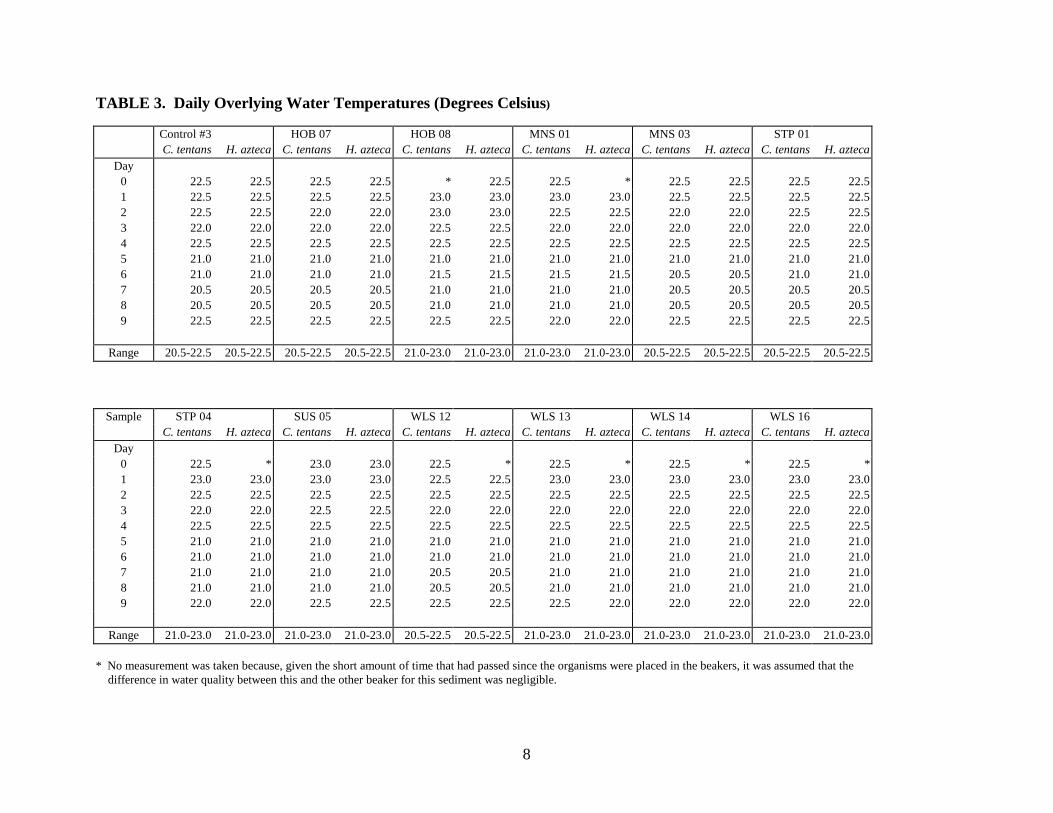
8

TABLE 3. Daily Overlying Water Temperatures (Degrees Celsius)

Control #3 HOB 07 HOB 08 MNS 01 MNS 03 STP 01C. tentans H. azteca C. tentans H. azteca C. tentans H. azteca C. tentans H. azteca C. tentans H. azteca C. tentans H. azteca

Day0 22.5 22.5 22.5 22.5 * 22.5 22.5 * 22.5 22.5 22.5 22.51 22.5 22.5 22.5 22.5 23.0 23.0 23.0 23.0 22.5 22.5 22.5 22.52 22.5 22.5 22.0 22.0 23.0 23.0 22.5 22.5 22.0 22.0 22.5 22.53 22.0 22.0 22.0 22.0 22.5 22.5 22.0 22.0 22.0 22.0 22.0 22.04 22.5 22.5 22.5 22.5 22.5 22.5 22.5 22.5 22.5 22.5 22.5 22.55 21.0 21.0 21.0 21.0 21.0 21.0 21.0 21.0 21.0 21.0 21.0 21.06 21.0 21.0 21.0 21.0 21.5 21.5 21.5 21.5 20.5 20.5 21.0 21.07 20.5 20.5 20.5 20.5 21.0 21.0 21.0 21.0 20.5 20.5 20.5 20.58 20.5 20.5 20.5 20.5 21.0 21.0 21.0 21.0 20.5 20.5 20.5 20.59 22.5 22.5 22.5 22.5 22.5 22.5 22.0 22.0 22.5 22.5 22.5 22.5

Range 20.5-22.5 20.5-22.5 20.5-22.5 20.5-22.5 21.0-23.0 21.0-23.0 21.0-23.0 21.0-23.0 20.5-22.5 20.5-22.5 20.5-22.5 20.5-22.5

Sample STP 04 SUS 05 WLS 12 WLS 13 WLS 14 WLS 16C. tentans H. azteca C. tentans H. azteca C. tentans H. azteca C. tentans H. azteca C. tentans H. azteca C. tentans H. azteca

Day0 22.5 * 23.0 23.0 22.5 * 22.5 * 22.5 * 22.5 *1 23.0 23.0 23.0 23.0 22.5 22.5 23.0 23.0 23.0 23.0 23.0 23.02 22.5 22.5 22.5 22.5 22.5 22.5 22.5 22.5 22.5 22.5 22.5 22.53 22.0 22.0 22.5 22.5 22.0 22.0 22.0 22.0 22.0 22.0 22.0 22.04 22.5 22.5 22.5 22.5 22.5 22.5 22.5 22.5 22.5 22.5 22.5 22.55 21.0 21.0 21.0 21.0 21.0 21.0 21.0 21.0 21.0 21.0 21.0 21.06 21.0 21.0 21.0 21.0 21.0 21.0 21.0 21.0 21.0 21.0 21.0 21.07 21.0 21.0 21.0 21.0 20.5 20.5 21.0 21.0 21.0 21.0 21.0 21.08 21.0 21.0 21.0 21.0 20.5 20.5 21.0 21.0 21.0 21.0 21.0 21.09 22.0 22.0 22.5 22.5 22.5 22.5 22.5 22.0 22.0 22.0 22.0 22.0

Range 21.0-23.0 21.0-23.0 21.0-23.0 21.0-23.0 20.5-22.5 20.5-22.5 21.0-23.0 21.0-23.0 21.0-23.0 21.0-23.0 21.0-23.0 21.0-23.0

* No measurement was taken because, given the short amount of time that had passed since the organisms were placed in the beakers, it was assumed that the difference in water quality between this and the other beaker for this sediment was negligible.

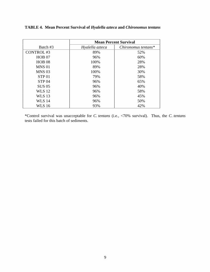
9

TABLE 4. Mean Percent Survival of Hyalella azteca and Chironomus tentans

Mean Percent SurvivalBatch #3 Hyalella azteca Chironomus tentans*

CONTROL #3 89% 52%HOB 07 96% 60%HOB 08 100% 28%MNS 01 89% 28%MNS 03 100% 30%STP 01 79% 58%STP 04 96% 65%SUS 05 96% 40%

WLS 12 96% 58%WLS 13 96% 45%WLS 14 96% 50%WLS 16 93% 42%

*Control survival was unacceptable for C. tentans (i.e., <70% survival). Thus, the C. tentanstests failed for this batch of sediments.

APPENDIX A

Statistical Analyses

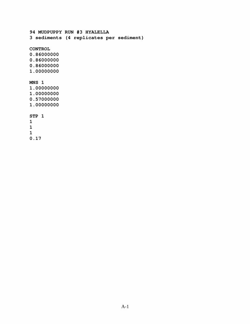
A-1

94 MUDPUPPY RUN #3 HYALELLA3 sediments (4 replicates per sediment)

CONTROL0.860000000.860000000.860000001.00000000

MNS 11.000000001.000000000.570000001.00000000

STP 11110.17

A-2

TITLE: 94 MUDPUPPY RUN #3 HYALELLAFILE: 94MUD3.DATTRANSFORM: ARC SINE(SQUARE ROOT(Y)) NUMBER OF GROUPS: 3----------------------------------------------------------------

GRP IDENTIFICATION REP VALUE TRANS VALUE--- ---------------- ---- ------------- -------------1 CONTROL 1 0.8600 1.18731 CONTROL 2 0.8600 1.18731 CONTROL 3 0.8600 1.18731 CONTROL 4 1.0000 1.41202 MNS 1 1 1.0000 1.41202 MNS 1 2 1.0000 1.41202 MNS 1 3 0.5700 0.85562 MNS 1 4 1.0000 1.41203 STP 1 1 1.0000 1.41203 STP 1 2 1.0000 1.41203 STP 1 3 1.0000 1.41203 STP 1 4 0.1700 0.4250----------------------------------------------------------------

94 MUDPUPPY RUN #3 HYALELLAFile: 94MUD3.DAT Transform: ARC SINE(SQUARE ROOT(Y))

SUMMARY STATISTICS ON TRANSFORMED DATA TABLE 1 of 2-----------------------------------------------------------------

GRP IDENTIFICATION N MIN MAX MEAN--- ---------------- ---- ---------- ---------- ----------1 CONTROL 4 1.187 1.412 1.2432 MNS 1 4 0.856 1.412 1.2733 STP 1 4 0.425 1.412 1.165-----------------------------------------------------------------

A-3

94 MUDPUPPY RUN #3 HYALELLAFile: 94MUD3.DAT Transform: ARC SINE(SQUARE ROOT(Y))

SUMMARY STATISTICS ON TRANSFORMED DATA TABLE 2 of 2----------------------------------------------------------------------

GRP IDENTIFICATION VARIANCE SD SEM C.V. %--- ---------------- -------------- ---------- ---------- ----------1 CONTROL 0.013 0.112 0.056 9.042 MNS 1 0.077 0.278 0.139 21.853 STP 1 0.244 0.494 0.247 42.35----------------------------------------------------------------------

94 MUDPUPPY RUN #3 HYALELLAFile: 94MUD3.DAT Transform: ARC SINE(SQUARE ROOT(Y))

Shapiro - Wilk's test for normality----------------------------------------------------------------------

D = 1.001

W = 0.784

Critical W (P = 0.05) (n = 12) = 0.859Critical W (P = 0.01) (n = 12) = 0.805----------------------------------------------------------------------

Data FAIL normality test. Try another transformation.

Warning: The first three homogeneity tests are sensitive to non-normaldata and should not be performed.

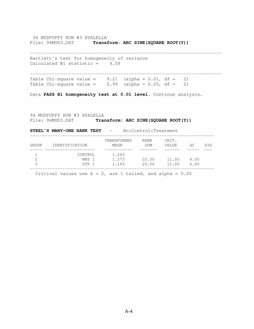
A-4

94 MUDPUPPY RUN #3 HYALELLAFile: 94MUD3.DAT Transform: ARC SINE(SQUARE ROOT(Y))

----------------------------------------------------------------------Bartlett's test for homogeneity of varianceCalculated B1 statistic = 4.58

----------------------------------------------------------------------Table Chi-square value = 9.21 (alpha = 0.01, df = 2)Table Chi-square value = 5.99 (alpha = 0.05, df = 2)

Data PASS B1 homogeneity test at 0.01 level. Continue analysis.

94 MUDPUPPY RUN #3 HYALELLAFile: 94MUD3.DAT Transform: ARC SINE(SQUARE ROOT(Y))

STEEL'S MANY-ONE RANK TEST - Ho:Control<Treatment--------------------------------------------------------------------------

TRANSFORMED RANK CRIT.GROUP IDENTIFICATION MEAN SUM VALUE df SIG----- -------------------- ----------- ------- ------ ----- ---

1 CONTROL 1.2432 MNS 1 1.273 20.50 11.00 4.003 STP 1 1.165 20.50 11.00 4.00

--------------------------------------------------------------------------Critical values use k = 2, are 1 tailed, and alpha = 0.05

ACUTE TOXICITY TESTSWITH

HYALELLA AZTECA AND CHIRONOMUS TENTANSON SEDIMENTS FROM THE DULUTH/SUPERIOR HARBOR:

1994 Sampling Results - Batch # 4

Conducted by

Minnesota Pollution Control AgencyMonitoring and Assessment Section

520 Lafayette RoadSt. Paul, Minnesota 55155-4194

April 1997

ii

TABLE OF CONTENTS

INTRODUCTION . . . . . . . . . . . . . . . . . . . . . . . . . . . . . . . . . . . . . . . . . . . . . . . . . . . . . . . . . . . . 1

SAMPLE COLLECTION AND HANDLING . . . . . . . . . . . . . . . . . . . . . . . . . . . . . . . . . . . . . . 1

METHODS . . . . . . . . . . . . . . . . . . . . . . . . . . . . . . . . . . . . . . . . . . . . . . . . . . . . . . . . . . . . . . . . . 1

RESULTS . . . . . . . . . . . . . . . . . . . . . . . . . . . . . . . . . . . . . . . . . . . . . . . . . . . . . . . . . . . . . . . . . . 2

SUMMARY . . . . . . . . . . . . . . . . . . . . . . . . . . . . . . . . . . . . . . . . . . . . . . . . . . . . . . . . . . . . . . . . 4

REFERENCES . . . . . . . . . . . . . . . . . . . . . . . . . . . . . . . . . . . . . . . . . . . . . . . . . . . . . . . . . . . . . . . 4

APPENDIX A - Statistical Analyses

iii

LIST OF TABLES

TABLE 1. Daily Overlying Water pH Measurements ..................................................................5

TABLE 2. Daily Overlying Water Dissolved Oxygen Concentrations (mg/L)............................. 6

TABLE 3. Daily Overlying Water Temperatures (Degrees Celsius)............................................ 7

TABLE 4. Mean Percent Survival of Hyalella azteca and Chironomus tentans .......................... 8

1

INTRODUCTION

As part of a sediment assessment of hotspot areas in the Duluth/Superior Harbor, sedimenttoxicity tests were conducted to assess acute (survival) and chronic (growth) toxicity to benthicinvertebrates. Acute effects were measured in separate 10-day toxicity tests to Hyalella azteca(H. azteca) and Chironomus tentans (C. tentans). Growth was measured at the end of theC. tentans test to assess chronic effects. Survival and growth endpoints were compared toorganisms similarly exposed to a reference control sediment collected from West Bearskin Lake(Cook County, MN).

A total of 44 sediment samples were collected for toxicity testing. This report presents theresults of six of these sediment samples.

SAMPLE COLLECTION AND HANDLING

During September 28-29, 1994, Minnesota Pollution Control Agency (MPCA) staff collected thesix sediments referred to in this report. The composited samples were collected from the harborusing a gravity corer. The samples were stored at 4°C at the Duluth MPCA office until they weretransported to the MPCA Toxicology Laboratory in St. Paul, MN.

METHODS

Six sediment samples and a control sediment were subjected to the 10-day sediment toxicity testusing the procedures described in U.S. EPA (1994). The test organisms (H. azteca andC. tentans) were exposed to sediment samples in a portable, mini-flow system described inBenoit et al. (1993) and U.S. EPA (1994). The test apparatus consists of 300 mL, glass-beakertest chambers held in a glass box supplied with water from an acrylic plastic headbox. Thebeakers have two, 1.5 cm holes covered with stainless steel mesh, to allow for water exchangewhile containing the test organisms. The headbox has a pipette tip drain calibrated to deliverwater at an average rate of 32.5 mL/min. The glass box is fitted with a self-starting siphon toprovide exchange of overlying water.

The H. azteca used for this test were 1 to 3 mm long, and the C. tentans were approximately14 days old. These organisms were supplied by Environmental Consulting and Testing(Superior, WI) prior to the test set up.

On November 1, 1994, six samples (HOB 10, HOB 11, HOB 12, HOB 13, HOB 14, andHOB 15) and the control sediment were separately homogenized by hand, and 100 mL of eachsediment was placed in a test beaker (Batch #4). Each sediment test was set up with fourreplicates of H. azteca and four replicates of C. tentans. Approximately 100 mL of aerated,artesian well water was added to the beakers, and the sediments were allowed to settle forapproximately two hours before the organisms were added. For each sediment, ten organismswere placed in each of eight beakers in a random fashion.

2

The organisms were exposed to 16 hours of light and eight hours of darkness for the duration ofthe ten-day test. Each day, two liters of aerated water from the artesian well at Stroh Brewery inSt. Paul, MN were exchanged in each test chamber. On weekdays, 1-L was exchanged in themorning and 1-L in the afternoon. On weekends, the two liters were passed through thechambers all at once. Water quality measurements (i.e., pH, temperature, and dissolved oxygen)of the overlying water were taken in one beaker of each of the quadruplicate sets of each of thesediments. The results, along with daily observations involving the physical appearance of thesediments and organisms, were recorded in a laboratory notebook. This notebook is retained onfile at the MPCA.

The test was terminated on November 11, 1994. The sediments were sieved through 40 meshscreens, and the sieved material was sorted for organisms. The organisms found were counted,and the number of alive and dead organisms were recorded. Organisms not found were recordedas missing and presumed dead. The C. tentans that survived were placed in aluminum weighingdishes, dried at approximately 100°C for at least four hours, desiccated to room temperature, andweighed.

Growth (weight) of the C. tentans and survival of both organisms were used as the endpoints forthese tests. The survival data were analyzed using TOXSTAT (Gulley and WEST, Inc., 1994), astatistical software package obtained from the University of Wyoming. However, due to aquality assurance problem, the growth data were not analyzed.

A 96-hour, reference toxicant test with H. azteca in sodium chloride (NaCl) was run inconjunction with these toxicity tests to determine the acceptability of the H. azteca used. Fourconcentrations of NaCl solution (i.e., 10, 5, 2.5, and 1.25 g/L) and a control (aerated, artesianwell water) were used in this test. Three replicates of five organisms each were set up perconcentration.

RESULTS

Water Quality

Measurements of pH, dissolved oxygen, and temperature in the overlying water of the testbeakers were made daily. These measurements are summarized below and in Tables 1, 2, and 3,respectively.

The range of pH values in the beakers containing H. azteca was 7.4 to 8.2 (Table 1). The waterin the C. tentans beakers had a pH range of 7.5 to 8.1 (Table 1). The pH fluctuations duringthese tests were acceptable since they did not vary more than 50% within each treatment(U.S. EPA, 1994).

The dissolved oxygen concentration ranged from 3.8 to 6.7 mg/L in the H. azteca beakers andfrom 2.2 to 6.4 mg/L in the C. tentans beakers (Table 2). It should be noted that on Days 3, 5, 8and 9, the dissolved oxygen concentration of the C. tentans beakers containing samples HOB 13,HOB 14, and HOB 15 was unacceptable (i.e., less than 40% saturated). Also, on Day 6, the

3

dissolved oxygen concentration of the water in the C. tentans beaker of HOB 14 wasunacceptable, as it was on Day 7 in the C. tentans beakers of HOB 13 and HOB 15. Theorganisms continued to be fed throughout the test.

The temperature of the overlying water in each glass box was measured and ranged from 20.5°Cto 23.0°C in both tests (Table 3). The recommended temperature for these tests is 23 ± 1°C(U.S. EPA, 1994).

Test Endpoints

Survival Data

The mean percent survival of the test organisms is summarized below and in Table 4.

The mean percent survival of H. azteca in the control was 88% with a range of 80% to 100%.For the control sediment containing C. tentans, percent survival ranged from 80% to 90% with amean of 88%. Survival for these controls was acceptable, and both tests passed.

Mean percent survival of H. azteca in the test sediments ranged from 52% in the HOB 13sediment to 95% in the HOB 10 sediment. Mean percent survival of C. tentans in the testsediments ranged from 70% in the HOB 11 and HOB 12 samples to 80% in the HOB 10, HOB14, and HOB 15 samples.

C. Tentans Growth Data

Although the dried C. tentans were weighed, the balance on which they were weighed was notcalibrated with standard weights. Therefore, the data are suspect since the internal calibration ofthe balance may have drifted with time. Thus, no conclusions can be made regarding chronictoxicity (growth).

Data Analysis

All data were transformed using an arc sine-square root transformation before being subjected tostatistical analysis. A one-tailed statistical test was used to test the alternative hypothesis thatsample survival was less than control survival. For H. azteca, Dunnett’s test was used todetermine that HOB 12 and HOB 13 had significantly lower survival than the control (p = 0.05).For C. tentans, a nonparametric statistical test (i.e., Steel’s Many-one Rank test) had to be useddue to 0% variance in the HOB 14 replicates. None of the C. tentans test sediments were toxiccompared to the control sediment (α = 0.05). The statistical analysis of these data is included inAppendix A.

4

Reference Toxicant Test with Hyalella azteca in Sodium Chloride Solution

Measurements of pH, dissolved oxygen, and temperature in the overlying water of the testvessels for this test were made daily for the tests 96-hour duration. A daily count of survivingorganisms in each vessel was also made.

The pH of the overlying water in the reference toxicant test ranged from 8.1 to 8.5. Thedissolved oxygen ranged from 7.6 to 8.3 mg/L, and the temperature of the overlying waterranged from 20.0°C to 21.8°C. The mean percent survival of the organisms in the control wasgreater than 90% (i.e., 100%) which was acceptable.

The LC50 for this reference toxicant test was 3.80 g/L NaCl as determined by the TrimmedSpearman-Karber method. A control chart will be developed for this test once five data pointsare obtained.

SUMMARY

Control survival of H. azteca in both the reference toxicant test and the sediment test wasacceptable (i.e., greater than 90% and 80%, respectively). Survival of H. azteca in the testsediments was statistically less than the control (p = 0.05) in only two samples: HOB 12 andHOB 13.

Control survival in the C. tentans test was acceptable (i.e., greater than 70%). Survival ofC. tentans in all of the test sediments was not significantly less than that of the control (α = 0.05).

REFERENCES

Benoit, D.A., G. Phipps, and G.T. Ankley. 1993. A sediment testing intermittent renewal system for the automated renewal of overlying water in toxicity tests with contaminated sediments. Water Research 27:1403-1412.

Gulley, D.D. and WEST, Inc. 1994. TOXSTAT 3.4. WEST, Inc., Cheyenne, WY.

U.S. EPA. 1994. Methods for measuring the toxicity and bioaccumulation of sediment-associated contaminants with freshwater invertebrates. Office of Research and Development, U.S. Environmental Protection Agency, Duluth, MN. EPA/600/R-94/024.

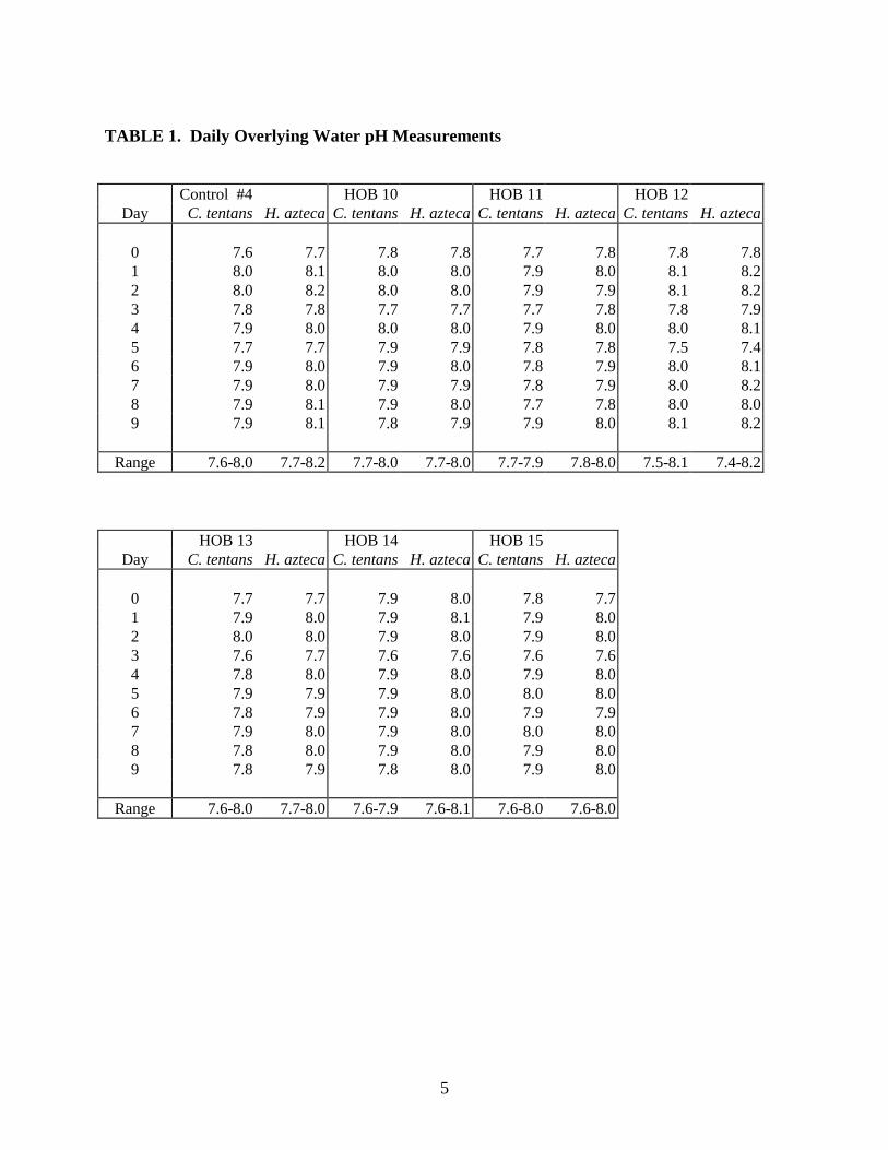
5

TABLE 1. Daily Overlying Water pH Measurements

Control #4 HOB 10 HOB 11 HOB 12Day C. tentans H. azteca C. tentans H. azteca C. tentans H. azteca C. tentans H. azteca

0 7.6 7.7 7.8 7.8 7.7 7.8 7.8 7.81 8.0 8.1 8.0 8.0 7.9 8.0 8.1 8.22 8.0 8.2 8.0 8.0 7.9 7.9 8.1 8.23 7.8 7.8 7.7 7.7 7.7 7.8 7.8 7.94 7.9 8.0 8.0 8.0 7.9 8.0 8.0 8.15 7.7 7.7 7.9 7.9 7.8 7.8 7.5 7.46 7.9 8.0 7.9 8.0 7.8 7.9 8.0 8.17 7.9 8.0 7.9 7.9 7.8 7.9 8.0 8.28 7.9 8.1 7.9 8.0 7.7 7.8 8.0 8.09 7.9 8.1 7.8 7.9 7.9 8.0 8.1 8.2

Range 7.6-8.0 7.7-8.2 7.7-8.0 7.7-8.0 7.7-7.9 7.8-8.0 7.5-8.1 7.4-8.2

HOB 13 HOB 14 HOB 15Day C. tentans H. azteca C. tentans H. azteca C. tentans H. azteca

0 7.7 7.7 7.9 8.0 7.8 7.71 7.9 8.0 7.9 8.1 7.9 8.02 8.0 8.0 7.9 8.0 7.9 8.03 7.6 7.7 7.6 7.6 7.6 7.64 7.8 8.0 7.9 8.0 7.9 8.05 7.9 7.9 7.9 8.0 8.0 8.06 7.8 7.9 7.9 8.0 7.9 7.97 7.9 8.0 7.9 8.0 8.0 8.08 7.8 8.0 7.9 8.0 7.9 8.09 7.8 7.9 7.8 8.0 7.9 8.0

Range 7.6-8.0 7.7-8.0 7.6-7.9 7.6-8.1 7.6-8.0 7.6-8.0

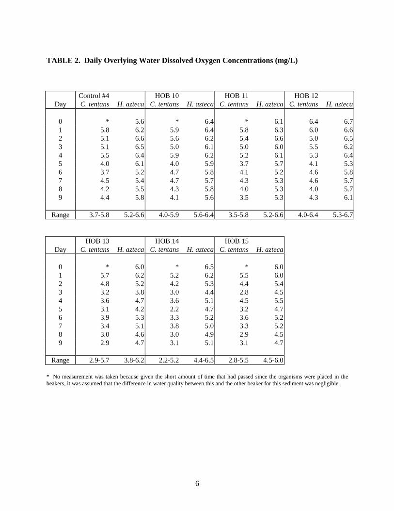
6

TABLE 2. Daily Overlying Water Dissolved Oxygen Concentrations (mg/L)

Control #4 HOB 10 HOB 11 HOB 12Day C. tentans H. azteca C. tentans H. azteca C. tentans H. azteca C. tentans H. azteca

0 * 5.6 * 6.4 * 6.1 6.4 6.71 5.8 6.2 5.9 6.4 5.8 6.3 6.0 6.62 5.1 6.6 5.6 6.2 5.4 6.6 5.0 6.53 5.1 6.5 5.0 6.1 5.0 6.0 5.5 6.24 5.5 6.4 5.9 6.2 5.2 6.1 5.3 6.45 4.0 6.1 4.0 5.9 3.7 5.7 4.1 5.36 3.7 5.2 4.7 5.8 4.1 5.2 4.6 5.87 4.5 5.4 4.7 5.7 4.3 5.3 4.6 5.78 4.2 5.5 4.3 5.8 4.0 5.3 4.0 5.79 4.4 5.8 4.1 5.6 3.5 5.3 4.3 6.1

Range 3.7-5.8 5.2-6.6 4.0-5.9 5.6-6.4 3.5-5.8 5.2-6.6 4.0-6.4 5.3-6.7

HOB 13 HOB 14 HOB 15Day C. tentans H. azteca C. tentans H. azteca C. tentans H. azteca

0 * 6.0 * 6.5 * 6.01 5.7 6.2 5.2 6.2 5.5 6.02 4.8 5.2 4.2 5.3 4.4 5.43 3.2 3.8 3.0 4.4 2.8 4.54 3.6 4.7 3.6 5.1 4.5 5.55 3.1 4.2 2.2 4.7 3.2 4.76 3.9 5.3 3.3 5.2 3.6 5.27 3.4 5.1 3.8 5.0 3.3 5.28 3.0 4.6 3.0 4.9 2.9 4.59 2.9 4.7 3.1 5.1 3.1 4.7

Range 2.9-5.7 3.8-6.2 2.2-5.2 4.4-6.5 2.8-5.5 4.5-6.0

* No measurement was taken because given the short amount of time that had passed since the organisms were placed in thebeakers, it was assumed that the difference in water quality between this and the other beaker for this sediment was negligible.

7

TABLE 3. Daily Overlying Water Temperatures (Degrees Celsius)

Control #4 HOB 10 HOB 11 HOB 12Day C. tentans H. azteca C. tentans H. azteca C. tentans H. azteca C. tentans H. azteca

0 21.0 21.0 21.5 21.5 21.0 21.0 21.5 21.51 21.5 21.5 21.5 21.5 21.5 21.5 22.0 22.02 21.5 21.5 21.0 21.0 21.0 21.0 21.5 21.53 21.0 21.0 21.0 21.0 21.0 21.0 21.0 21.04 22.5 22.5 22.0 22.0 22.0 22.0 23.0 23.05 23.0 23.0 22.0 22.0 23.0 23.0 23.0 23.06 21.5 21.5 21.5 21.5 21.5 21.5 22.0 22.07 21.0 21.0 21.0 21.0 21.0 21.0 21.5 21.58 21.0 21.0 20.5 20.5 21.0 21.0 21.0 21.09 20.7 20.7 20.8 20.8 20.8 20.8 21.0 21.0

Range 20.7-23.0 20.7-23.0 20.5-22.0 20.5-22.0 20.8-23.0 20.8-23.0 21.0-23.0 21.0-23.0

HOB 13 HOB 14 HOB 15Day C. tentans H. azteca C. tentans H. azteca C. tentans H. azteca

0 21.5 21.5 21.5 21.5 21.5 21.51 21.5 21.5 22.5 22.5 21.5 21.52 21.0 21.0 22.0 22.0 21.0 21.03 21.0 21.0 21.0 21.0 21.0 21.04 22.0 22.0 23.0 23.0 22.5 22.55 22.0 22.0 23.0 23.0 23.0 23.06 21.5 21.5 22.0 22.0 21.5 21.57 21.0 21.0 22.0 22.0 21.0 21.08 20.5 20.5 21.5 21.5 20.5 20.59 20.6 20.6 21.5 21.5 20.8 20.8

Range 20.5-22.0 20.5-22.0 21.0-23.0 21.0-23.0 20.5-23.0 20.5-23.0

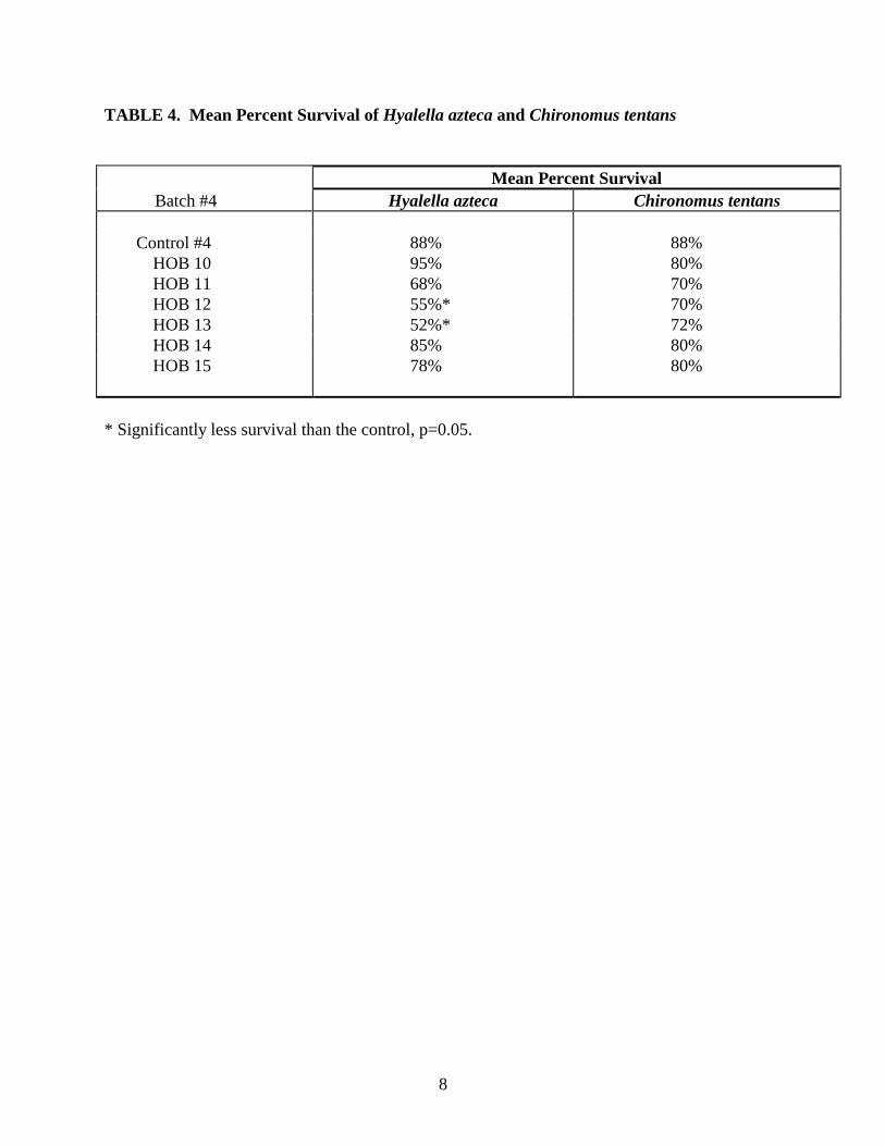
8

TABLE 4. Mean Percent Survival of Hyalella azteca and Chironomus tentans

Mean Percent SurvivalB Batch #4 Hyalella azteca Chironomus tentans

Control #4 88% 88%HOB 10 95% 80%HOB 11 68% 70%HOB 12 55%* 70%HOB 13 52%* 72%HOB 14 85% 80%HOB 15 78% 80%

* Significantly less survival than the control, p=0.05.

APPENDIX A

Statistical Analyses

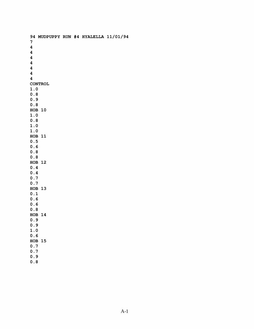
A-1

94 MUDPUPPY RUN #4 HYALELLA 11/01/9474444444CONTROL1.00.80.90.8HOB 101.00.81.01.0HOB 110.50.60.80.8HOB 120.40.40.70.7HOB 130.10.60.60.8HOB 140.90.91.00.6HOB 150.70.70.90.8

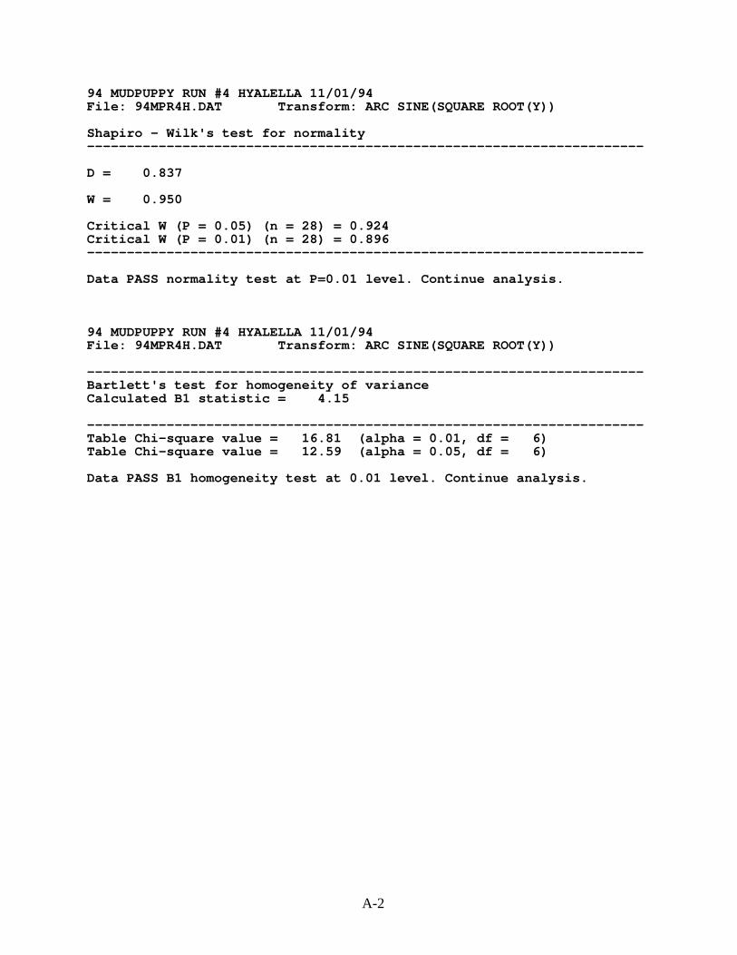
A-2

94 MUDPUPPY RUN #4 HYALELLA 11/01/94File: 94MPR4H.DAT Transform: ARC SINE(SQUARE ROOT(Y))

Shapiro - Wilk's test for normality----------------------------------------------------------------------

D = 0.837

W = 0.950

Critical W (P = 0.05) (n = 28) = 0.924Critical W (P = 0.01) (n = 28) = 0.896----------------------------------------------------------------------

Data PASS normality test at P=0.01 level. Continue analysis.

94 MUDPUPPY RUN #4 HYALELLA 11/01/94File: 94MPR4H.DAT Transform: ARC SINE(SQUARE ROOT(Y))

----------------------------------------------------------------------Bartlett's test for homogeneity of varianceCalculated B1 statistic = 4.15

----------------------------------------------------------------------Table Chi-square value = 16.81 (alpha = 0.01, df = 6)Table Chi-square value = 12.59 (alpha = 0.05, df = 6)

Data PASS B1 homogeneity test at 0.01 level. Continue analysis.

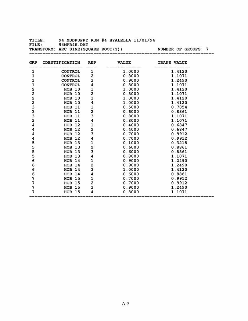
A-3

TITLE: 94 MUDPUPPY RUN #4 HYALELLA 11/01/94FILE: 94MPR4H.DATTRANSFORM: ARC SINE(SQUARE ROOT(Y)) NUMBER OF GROUPS: 7---------------------------------------------------------------------

GRP IDENTIFICATION REP VALUE TRANS VALUE--- ---------------- ---- ------------- -------------1 CONTROL 1 1.0000 1.41201 CONTROL 2 0.8000 1.10711 CONTROL 3 0.9000 1.24901 CONTROL 4 0.8000 1.10712 HOB 10 1 1.0000 1.41202 HOB 10 2 0.8000 1.10712 HOB 10 3 1.0000 1.41202 HOB 10 4 1.0000 1.41203 HOB 11 1 0.5000 0.78543 HOB 11 2 0.6000 0.88613 HOB 11 3 0.8000 1.10713 HOB 11 4 0.8000 1.10714 HOB 12 1 0.4000 0.68474 HOB 12 2 0.4000 0.68474 HOB 12 3 0.7000 0.99124 HOB 12 4 0.7000 0.99125 HOB 13 1 0.1000 0.32185 HOB 13 2 0.6000 0.88615 HOB 13 3 0.6000 0.88615 HOB 13 4 0.8000 1.10716 HOB 14 1 0.9000 1.24906 HOB 14 2 0.9000 1.24906 HOB 14 3 1.0000 1.41206 HOB 14 4 0.6000 0.88617 HOB 15 1 0.7000 0.99127 HOB 15 2 0.7000 0.99127 HOB 15 3 0.9000 1.24907 HOB 15 4 0.8000 1.1071

---------------------------------------------------------------------

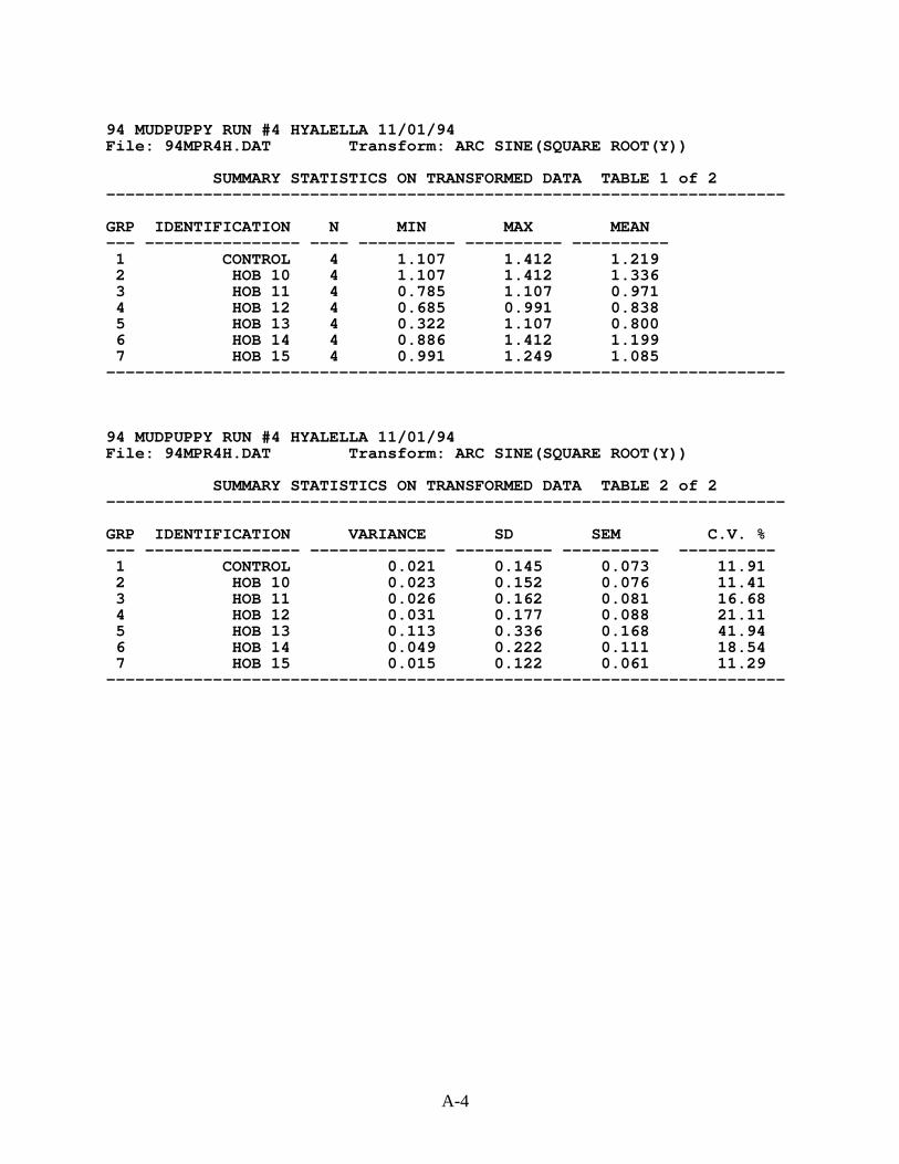
A-4

94 MUDPUPPY RUN #4 HYALELLA 11/01/94File: 94MPR4H.DAT Transform: ARC SINE(SQUARE ROOT(Y))

SUMMARY STATISTICS ON TRANSFORMED DATA TABLE 1 of 2----------------------------------------------------------------------

GRP IDENTIFICATION N MIN MAX MEAN--- ---------------- ---- ---------- ---------- ----------1 CONTROL 4 1.107 1.412 1.2192 HOB 10 4 1.107 1.412 1.3363 HOB 11 4 0.785 1.107 0.9714 HOB 12 4 0.685 0.991 0.8385 HOB 13 4 0.322 1.107 0.8006 HOB 14 4 0.886 1.412 1.1997 HOB 15 4 0.991 1.249 1.085

----------------------------------------------------------------------

94 MUDPUPPY RUN #4 HYALELLA 11/01/94File: 94MPR4H.DAT Transform: ARC SINE(SQUARE ROOT(Y))

SUMMARY STATISTICS ON TRANSFORMED DATA TABLE 2 of 2----------------------------------------------------------------------

GRP IDENTIFICATION VARIANCE SD SEM C.V. %--- ---------------- -------------- ---------- ---------- ----------1 CONTROL 0.021 0.145 0.073 11.912 HOB 10 0.023 0.152 0.076 11.413 HOB 11 0.026 0.162 0.081 16.684 HOB 12 0.031 0.177 0.088 21.115 HOB 13 0.113 0.336 0.168 41.946 HOB 14 0.049 0.222 0.111 18.547 HOB 15 0.015 0.122 0.061 11.29

----------------------------------------------------------------------

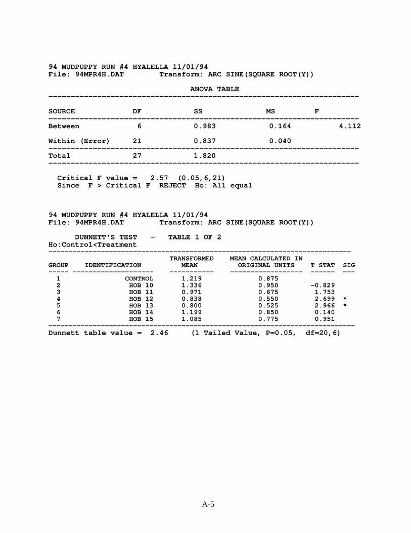
A-5

94 MUDPUPPY RUN #4 HYALELLA 11/01/94File: 94MPR4H.DAT Transform: ARC SINE(SQUARE ROOT(Y))

ANOVA TABLE----------------------------------------------------------------------

SOURCE DF SS MS F----------------------------------------------------------------------Between 6 0.983 0.164 4.112

Within (Error) 21 0.837 0.040----------------------------------------------------------------------Total 27 1.820----------------------------------------------------------------------

Critical F value = 2.57 (0.05,6,21)Since F > Critical F REJECT Ho: All equal

94 MUDPUPPY RUN #4 HYALELLA 11/01/94File: 94MPR4H.DAT Transform: ARC SINE(SQUARE ROOT(Y))

DUNNETT'S TEST - TABLE 1 OF 2Ho:Control<Treatment---------------------------------------------------------------------------

TRANSFORMED MEAN CALCULATED INGROUP IDENTIFICATION MEAN ORIGINAL UNITS T STAT SIG----- -------------------- ----------- ------------------ ------ ---1 CONTROL 1.219 0.8752 HOB 10 1.336 0.950 -0.8293 HOB 11 0.971 0.675 1.7534 HOB 12 0.838 0.550 2.699 *5 HOB 13 0.800 0.525 2.966 *6 HOB 14 1.199 0.850 0.1407 HOB 15 1.085 0.775 0.951

----------------------------------------------------------------------------Dunnett table value = 2.46 (1 Tailed Value, P=0.05, df=20,6)

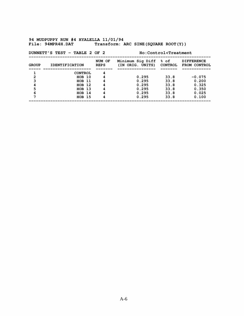
A-6

94 MUDPUPPY RUN #4 HYALELLA 11/01/94File: 94MPR4H.DAT Transform: ARC SINE(SQUARE ROOT(Y))

DUNNETT'S TEST - TABLE 2 OF 2 Ho:Control<Treatment----------------------------------------------------------------------------

NUM OF Minimum Sig Diff % of DIFFERENCEGROUP IDENTIFICATION REPS (IN ORIG. UNITS) CONTROL FROM CONTROL----- -------------------- ------- ---------------- ------- ------------1 CONTROL 42 HOB 10 4 0.295 33.8 -0.0753 HOB 11 4 0.295 33.8 0.2004 HOB 12 4 0.295 33.8 0.3255 HOB 13 4 0.295 33.8 0.3506 HOB 14 4 0.295 33.8 0.0257 HOB 15 4 0.295 33.8 0.100

----------------------------------------------------------------------------

A-7

94 MUDPUPPY RUN #4 CHIRONOMIDS 11/01/9474444444CONTROL0.800000000.900000000.900000000.90000000HOB 101.000000000.400000000.900000000.90000000HOB 110.500000000.600000000.900000000.80000000HOB 120.800000000.700000000.800000000.50000000HOB 130.800000000.800000000.400000000.90000000HOB 140.80.800000000.80.80000000HOB 150.70.80.90.8

A-8

File: S:\MA\CHUBBAR\TSD\94MUD\94MPR4C.DATTransform: ARC SINE(SQUARE ROOT(Y))

Shapiro - Wilk's test for normality----------------------------------------------------------------------

D = 0.734

W = 0.917

Critical W (P = 0.05) (n = 28) = 0.924Critical W (P = 0.01) (n = 28) = 0.896----------------------------------------------------------------------

Data PASS normality test at P=0.01 level. Continue analysis.

94 MUDPUPPY RUN #4 CHIRONOMIDS 11/01/94File: S:\MA\CHUBBAR\TSD\94MUD\94MPR4C.DATTransform: ARC SINE(SQUARE ROOT(Y))

Hartley's test for homogeneity of varianceBartlett's test for homogeneity of variance----------------------------------------------------------------------

These two tests can not be performed because at least one group haszero variance.

Data FAIL to meet homogeneity of variance assumption.Additional transformations are useless.

----------------------------------------------------------------------

A-9

TITLE: 94 MUDPUPPY RUN #4 CHIRONOMIDS 11/01/94FILE: S:\MA\CHUBBAR\TSD\94MUD\94MPR4C.DATTRANSFORM: ARC SINE(SQUARE ROOT(Y)) NUMBER OF GROUPS: 7----------------------------------------------------------------------

GRP IDENTIFICATION REP VALUE TRANS VALUE--- ---------------- ---- ------------- -------------1 CONTROL 1 0.8000 1.10711 CONTROL 2 0.9000 1.24901 CONTROL 3 0.9000 1.24901 CONTROL 4 0.9000 1.24902 HOB 10 1 1.0000 1.41202 HOB 10 2 0.4000 0.68472 HOB 10 3 0.9000 1.24902 HOB 10 4 0.9000 1.24903 HOB 11 1 0.5000 0.78543 HOB 11 2 0.6000 0.88613 HOB 11 3 0.9000 1.24903 HOB 11 4 0.8000 1.10714 HOB 12 1 0.8000 1.10714 HOB 12 2 0.7000 0.99124 HOB 12 3 0.8000 1.10714 HOB 12 4 0.5000 0.78545 HOB 13 1 0.8000 1.10715 HOB 13 2 0.8000 1.10715 HOB 13 3 0.4000 0.68475 HOB 13 4 0.9000 1.24906 HOB 14 1 0.8000 1.10716 HOB 14 2 0.8000 1.10716 HOB 14 3 0.8000 1.10716 HOB 14 4 0.8000 1.10717 HOB 15 1 0.7000 0.99127 HOB 15 2 0.8000 1.10717 HOB 15 3 0.9000 1.24907 HOB 15 4 0.8000 1.1071

----------------------------------------------------------------------

A-10

94 MUDPUPPY RUN #4 CHIRONOMIDS 11/01/94File: S:\MA\CHUBBAR\TSD\94MUD\94MPR4C.DATTransform: ARC SINE(SQUARE ROOT(Y))

SUMMARY STATISTICS ON TRANSFORMED DATA TABLE 1 of 2----------------------------------------------------------------------

GRP IDENTIFICATION N MIN MAX MEAN--- ---------------- ---- ---------- ---------- ----------1 CONTROL 4 1.107 1.249 1.2142 HOB 10 4 0.685 1.412 1.1493 HOB 11 4 0.785 1.249 1.0074 HOB 12 4 0.785 1.107 0.9985 HOB 13 4 0.685 1.249 1.0376 HOB 14 4 1.107 1.107 1.1077 HOB 15 4 0.991 1.249 1.114

----------------------------------------------------------------------

94 MUDPUPPY RUN #4 CHIRONOMIDS 11/01/94File: S:\MA\CHUBBAR\TSD\94MUD\94MPR4C.DATTransform: ARC SINE(SQUARE ROOT(Y))

SUMMARY STATISTICS ON TRANSFORMED DATA TABLE 2 of 2----------------------------------------------------------------------

GRP IDENTIFICATION VARIANCE SD SEM C.V. %--- ---------------- -------------- ---------- ---------- ----------1 CONTROL 0.005 0.071 0.035 5.852 HOB 10 0.102 0.319 0.159 27.753 HOB 11 0.044 0.210 0.105 20.864 HOB 12 0.023 0.152 0.076 15.215 HOB 13 0.060 0.244 0.122 23.556 HOB 14 0.000 0.000 0.000 0.007 HOB 15 0.011 0.106 0.053 9.48

----------------------------------------------------------------------

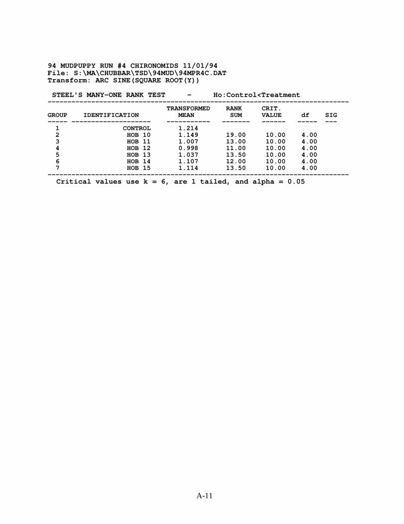
A-11

94 MUDPUPPY RUN #4 CHIRONOMIDS 11/01/94File: S:\MA\CHUBBAR\TSD\94MUD\94MPR4C.DATTransform: ARC SINE(SQUARE ROOT(Y))

STEEL'S MANY-ONE RANK TEST - Ho:Control<Treatment----------------------------------------------------------------------------

TRANSFORMED RANK CRIT.GROUP IDENTIFICATION MEAN SUM VALUE df SIG----- -------------------- ----------- ------- ------ ----- ---1 CONTROL 1.2142 HOB 10 1.149 19.00 10.00 4.003 HOB 11 1.007 13.00 10.00 4.004 HOB 12 0.998 11.00 10.00 4.005 HOB 13 1.037 13.50 10.00 4.006 HOB 14 1.107 12.00 10.00 4.007 HOB 15 1.114 13.50 10.00 4.00

----------------------------------------------------------------------------Critical values use k = 6, are 1 tailed, and alpha = 0.05

ACUTE TOXICITY TESTSWITH

HYALELLA AZTECA AND CHIRONOMUS TENTANSON SEDIMENTS FROM THE DULUTH/SUPERIOR HARBOR:

1994 Sampling Results - Batch # 5

Conducted by

Minnesota Pollution Control AgencyMonitoring and Assessment Section

520 Lafayette RoadSt. Paul, Minnesota 55155-4194

April 1997

ii

TABLE OF CONTENTS

INTRODUCTION . . . . . . . . . . . . . . . . . . . . . . . . . . . . . . . . . . . . . . . . . . . . . . . . . . . . . . . . . . . . 1

SAMPLE COLLECTION AND HANDLING . . . . . . . . . . . . . . . . . . . . . . . . . . . . . . . . . . . . . . 1

METHODS . . . . . . . . . . . . . . . . . . . . . . . . . . . . . . . . . . . . . . . . . . . . . . . . . . . . . . . . . . . . . . . . . 1

RESULTS . . . . . . . . . . . . . . . . . . . . . . . . . . . . . . . . . . . . . . . . . . . . . . . . . . . . . . . . . . . . . . . . . . 2

SUMMARY . . . . . . . . . . . . . . . . . . . . . . . . . . . . . . . . . . . . . . . . . . . . . . . . . . . . . . . . . . . . . . . . 4

REFERENCES . . . . . . . . . . . . . . . . . . . . . . . . . . . . . . . . . . . . . . . . . . . . . . . . . . . . . . . . . . . . . . . 4

iii

LIST OF TABLES

TABLE 1. Daily Overlying Water pH Measurements ..................................................................5

TABLE 2. Daily Overlying Water Dissolved Oxygen Concentrations (mg/L)............................. 6

TABLE 3. Daily Overlying Water Temperatures (Degrees Celsius) ........................................... 7

TABLE 4. Mean Percent Survival of Hyalella azteca and Chironomus tentans .......................... 8

1

INTRODUCTION

As part of a sediment assessment of hotspot areas in the Duluth/Superior Harbor, sedimenttoxicity tests were conducted to assess acute (survival) and chronic (growth) toxicity to benthicinvertebrates. Acute effects were measured in separate 10-day toxicity tests to Hyalella azteca(H. azteca) and Chironomus tentans (C. tentans). Growth was measured at the end of theC. tentans test to assess chronic effects. Survival and growth endpoints were compared toorganisms similarly exposed to a reference control sediment collected from West Bearskin Lake(Cook County, MN).

A total of 44 sediment samples were collected for toxicity testing. This report presents theresults of six of these sediment samples.

SAMPLE COLLECTION AND HANDLING

During October 3-4, 1994, Minnesota Pollution Control Agency (MPCA) staff collected the sixsediments referred to in this report. The samples were collected from the harbor using a gravitycorer. The samples were stored at 4°C at the Duluth MPCA office until they were transported tothe MPCA Toxicology Laboratory in St. Paul, MN.

METHODS

Six sediment samples and a control sediment were subjected to the 10-day sediment toxicity testusing the procedures described in U.S. EPA (1994). The test organisms (H. azteca andC. tentans) were exposed to sediment samples in a portable, mini-flow system described inBenoit et al. (1993) and U.S. EPA (1994). The test apparatus consists of 300 mL, glass-beakertest chambers held in a glass box supplied with water from an acrylic plastic headbox. Thebeakers have two, 1.5 cm holes covered with stainless steel mesh, to allow for water exchangewhile containing the test organisms. The headbox has a pipette tip drain calibrated to deliverwater at an average rate of 32.5 mL/min. The glass box is fitted with a self-starting siphon toprovide exchange of overlying water.

The H. azteca used for this test were 1 to 3 mm long, and the C. tentans were approximately 14days old. These organisms were supplied by Environmental Consulting and Testing (Superior,WI) prior to the test set up.

On November 11, 1994, six samples (ERP 03, KMB 04, KMB 05, STP 06, STP 07, and SUS 07)and the control sediment were separately homogenized by hand, and 100 mL of each sedimentwas placed in a test beaker (Batch #5). Approximately 100 mL of aerated, artesian well waterwas added to each beaker, and the sediments were allowed to settle for approximately two hoursbefore the organisms were added. Each sediment was set up with four replicates of H. azteca andfour replicates of C. Tentans. For each sediment, ten organisms were placed in each beaker in arandom fashion.

2

The organisms were exposed to 16 hours of light and eight hours of darkness for the duration ofthe ten-day test. Each day, two liters of aerated water from the artesian well at Stroh Brewery inSt. Paul, MN were exchanged in each test chamber. On weekdays, 1-L was exchanged in themorning and 1-L in the afternoon. On weekends, the two liters were passed through thechambers all at once. Water quality measurements (i.e., pH, temperature, and dissolved oxygen)of the overlying water were taken in one beaker of each of the quadruplicate sets of each of thesediments. The results, along with daily observations involving the physical appearance of thesediments and organisms, were recorded in a laboratory notebook. This notebook is retained onfile at the MPCA.

The test was terminated on November 21, 1994. The sediments were sieved through 40 meshscreens, and the sieved material was sorted for organisms. The organisms found were counted,and the number of alive and dead organisms were recorded. Organisms not found were recordedas missing and presumed dead. The C. tentans that survived were placed in aluminum weighingdishes, dried at approximately 100°C for at least four hours, desiccated to room temperature, andweighed.

Growth (weight) of the C. tentans and survival of both organisms were used as the endpoints forthese tests. Usually, the resulting data are analyzed using TOXSTAT (Gulley and WEST, Inc.,1994), a statistical software package obtained from the University of Wyoming. However, thecontrols failed for both of these tests which invalidated the survival data. Due to a qualityassurance problem, the growth data were not analyzed.

A 96-hour, reference toxicant test with H. azteca in sodium chloride (NaCl) was run inconjunction with these toxicity tests to determine the acceptability of the H. azteca used. Fourconcentrations of NaCl solution (i.e., 10, 5, 2.5, and 1.25 g/L) and a control (aerated, artesianwell water) were used in this test. Three replicates of five organisms each were set up perconcentration.

RESULTS

Water Quality

Measurements of pH, dissolved oxygen, and temperature in the overlying water of the testbeakers were made daily. These measurements are summarized below and in Tables 1, 2, and 3,respectively.

The range of pH values in the beakers containing H. azteca was 7.2 to 8.5 (Table 1). The waterin the C. tentans beakers had a pH range of 7.4 to 8.4 (Table 1). The pH fluctuations duringthese tests were acceptable since they did not vary more than 50% within each treatment(U.S. EPA, 1994).

The dissolved oxygen concentration ranged from 2.8 to 6.9 mg/L in the H. azteca beakers andfrom 1.8 to 6.7 mg/L in the C. tentans beakers (Table 2). It should be noted that on Days 4, 7, 8,and 9, the dissolved oxygen concentration in the STP 06 sediment beaker containing C. tentans

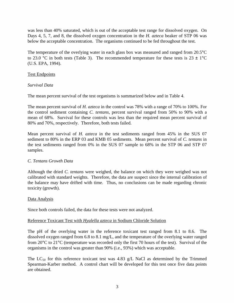
3

was less than 40% saturated, which is out of the acceptable test range for dissolved oxygen. OnDays 4, 5, 7, and 8, the dissolved oxygen concentration in the H. azteca beaker of STP 06 wasbelow the acceptable concentration. The organisms continued to be fed throughout the test.

The temperature of the overlying water in each glass box was measured and ranged from 20.5°Cto 23.0 °C in both tests (Table 3). The recommended temperature for these tests is 23 ± 1°C(U.S. EPA, 1994).

Test Endpoints

Survival Data

The mean percent survival of the test organisms is summarized below and in Table 4.

The mean percent survival of H. azteca in the control was 78% with a range of 70% to 100%. Forthe control sediment containing C. tentans, percent survival ranged from 50% to 90% with amean of 68%. Survival for these controls was less than the required mean percent survival of80% and 70%, respectively. Therefore, both tests failed.

Mean percent survival of H. azteca in the test sediments ranged from 45% in the SUS 07sediment to 80% in the ERP 03 and KMB 05 sediments. Mean percent survival of C. tentans inthe test sediments ranged from 0% in the SUS 07 sample to 68% in the STP 06 and STP 07samples.

C. Tentans Growth Data

Although the dried C. tentans were weighed, the balance on which they were weighed was notcalibrated with standard weights. Therefore, the data are suspect since the internal calibration ofthe balance may have drifted with time. Thus, no conclusions can be made regarding chronictoxicity (growth).

Data Analysis

Since both controls failed, the data for these tests were not analyzed.

Reference Toxicant Test with Hyalella azteca in Sodium Chloride Solution

The pH of the overlying water in the reference toxicant test ranged from 8.1 to 8.6. Thedissolved oxygen ranged from 6.8 to 8.1 mg/L, and the temperature of the overlying water rangedfrom 20°C to 21°C (temperature was recorded only the first 70 hours of the test). Survival of theorganisms in the control was greater than 90% (i.e., 93%) which was acceptable.

The LC50 for this reference toxicant test was 4.83 g/L NaCl as determined by the TrimmedSpearman-Karber method. A control chart will be developed for this test once five data pointsare obtained.

4

SUMMARY

Survival of the H. azteca in the reference toxicant test was acceptable (i.e., greater than 90%),indicating that the H. azteca organisms used in the toxicity test were healthy. However, survivalof H. azteca in the control sediments was unacceptable (i.e., less than 80%). Therefore, thetoxicity test failed.

Control survival was unacceptable in the C. tentans test (i.e., less than 70%), resulting in thefailure of this test.

REFERENCES

Benoit, D.A., G. Phipps, and G.T. Ankley. 1993. A sediment testing intermittent renewal system for the automated renewal of overlying water in toxicity tests with contaminated sediments. Water Research 27:1403-1412.

Gulley, D.D. and WEST, Inc. 1994. TOXSTAT 3.4. WEST, Inc., Cheyenne, WY.

U.S. EPA. 1994. Methods for measuring the toxicity and bioaccumulation of sediment-associated contaminants with freshwater invertebrates. Office of Research and Development, U.S. Environmental Protection Agency, Duluth, MN. EPA/600/R-94/024.

5

TABLE 1. Daily Overlying Water pH Measurements

Control #5 ERP 03 KMB 04 KMB 05Day C. tentans H. azteca C. tentans H. azteca C. tentans H. azteca C. tentans H. azteca

0 8.0 8.0 7.9 8.0 7.7 7.8 7.9 8.01 7.8 7.8 7.8 7.8 7.9 7.9 7.8 7.82 7.9 7.9 7.8 7.8 7.9 7.9 7.8 7.83 8.1 8.2 8.1 8.1 8.4 8.5 7.8 8.04 8.0 8.1 8.1 8.2 8.0 8.1 8.0 7.95 8.1 8.0 8.0 8.1 8.0 8.1 7.9 8.06 7.9 8.0 8.0 8.0 8.0 8.3 7.8 7.97 7.9 7.9 7.9 7.8 7.9 8.0 7.8 7.98 7.6 7.7 7.7 7.7 7.5 7.4 7.5 7.69 7.8 8.0 * * 7.7 7.9 * *

Range 7.6-8.1 7.7-8.2 7.7-8.1 7.7-8.2 7.5-8.4 7.4-8.5 7.5-7.9 7.6-8.0

STP 06 STP 07 SUS 07Day C. tentans H. azteca C. tentans H. azteca C. tentans H. azteca

0 7.8 7.9 7.9 8.0 7.4 7.21 7.9 7.9 7.8 7.8 8.2 8.12 7.9 7.9 7.8 7.8 8.0 8.13 8.2 8.3 8.1 8.2 8.4 8.44 7.9 8.0 8.0 8.0 8.2 7.85 7.8 8.0 8.0 8.2 8.2 8.26 8.0 8.0 8.0 8.0 8.2 8.17 7.9 7.9 7.8 7.7 8.1 8.28 7.7 7.6 7.6 7.6 7.7 7.49 7.8 7.9 * 8.0 7.9 7.7

Range 7.7-8.2 7.6-8.3 7.6-8.1 7.6-8.2 7.4-8.4 7.2-8.4

* pH meter was dropped and reading was questionable.

6

TABLE 2. Daily Overlying Water Dissolved Oxygen Concentrations (mg/L)

Control #5 ERP 03 KMB 04 KMB 05Day C. tentans H. azteca C. tentans H. azteca C. tentans H. azteca C. tentans H. azteca

0 6.7 6.7 6.4 6.4 6.2 6.1 6.7 6.91 5.8 6.2 5.8 6.2 6.3 6.0 4.6 5.02 5.5 5.8 5.9 6.2 6.0 6.2 6.0 6.13 5.9 6.0 6.1 5.8 5.8 5.9 6.0 6.04 5.5 6.0 6.3 5.6 6.1 6.1 6.2 5.75 5.9 5.5 6.4 5.6 6.2 5.2 6.1 5.76 5.7 5.4 5.9 6.3 5.9 5.1 6.1 5.77 5.1 5.0 5.6 5.6 5.3 4.6 5.0 5.08 4.4 4.4 3.8 4.4 4.4 4.0 4.3 4.99 3.8 4.3 5.2 5.1 4.1 4.3 4.3 4.4

Range 3.8-6.7 4.3-6.7 3.8-6.4 4.4-6.4 4.1-6.3 4.0-6.2 4.3-6.7 4.4-6.9

STP 06 STP 07 SUS 07Day C. tentans H. azteca C. tentans H. azteca C. tentans H. azteca

0 6.6 6.7 6.5 6.8 4.2 3.81 5.3 5.6 5.4 5.5 4.2 5.32 5.7 6.0 6.0 6.2 5.0 5.53 4.1 4.0 6.0 6.1 5.2 4.34 3.0 2.8 6.3 5.9 5.3 5.65 4.6 3.2 5.9 5.6 4.7 5.26 4.0 3.9 5.9 5.4 5.6 5.57 2.9 3.2 5.3 5.1 5.3 5.48 2.6 3.2 4.2 4.7 4.4 5.29 1.8 4.3 4.2 5.0 5.0 4.9

Range 1.8-6.6 2.8-6.7 4.2-6.5 4.7-6.8 4.2-5.6 3.8-5.6

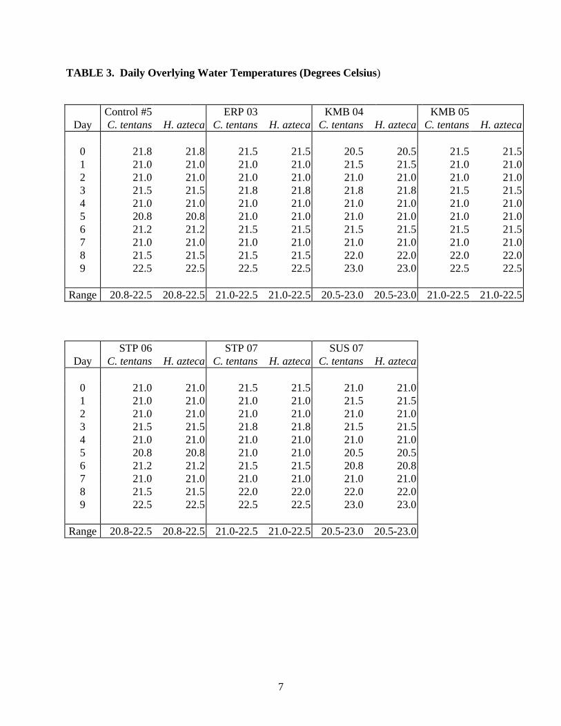
7

TABLE 3. Daily Overlying Water Temperatures (Degrees Celsius)

Control #5 ERP 03 KMB 04 KMB 05Day C. tentans H. azteca C. tentans H. azteca C. tentans H. azteca C. tentans H. azteca

0 21.8 21.8 21.5 21.5 20.5 20.5 21.5 21.51 21.0 21.0 21.0 21.0 21.5 21.5 21.0 21.02 21.0 21.0 21.0 21.0 21.0 21.0 21.0 21.03 21.5 21.5 21.8 21.8 21.8 21.8 21.5 21.54 21.0 21.0 21.0 21.0 21.0 21.0 21.0 21.05 20.8 20.8 21.0 21.0 21.0 21.0 21.0 21.06 21.2 21.2 21.5 21.5 21.5 21.5 21.5 21.57 21.0 21.0 21.0 21.0 21.0 21.0 21.0 21.08 21.5 21.5 21.5 21.5 22.0 22.0 22.0 22.09 22.5 22.5 22.5 22.5 23.0 23.0 22.5 22.5

Range 20.8-22.5 20.8-22.5 21.0-22.5 21.0-22.5 20.5-23.0 20.5-23.0 21.0-22.5 21.0-22.5

STP 06 STP 07 SUS 07Day C. tentans H. azteca C. tentans H. azteca C. tentans H. azteca

0 21.0 21.0 21.5 21.5 21.0 21.01 21.0 21.0 21.0 21.0 21.5 21.52 21.0 21.0 21.0 21.0 21.0 21.03 21.5 21.5 21.8 21.8 21.5 21.54 21.0 21.0 21.0 21.0 21.0 21.05 20.8 20.8 21.0 21.0 20.5 20.56 21.2 21.2 21.5 21.5 20.8 20.87 21.0 21.0 21.0 21.0 21.0 21.08 21.5 21.5 22.0 22.0 22.0 22.09 22.5 22.5 22.5 22.5 23.0 23.0

Range 20.8-22.5 20.8-22.5 21.0-22.5 21.0-22.5 20.5-23.0 20.5-23.0

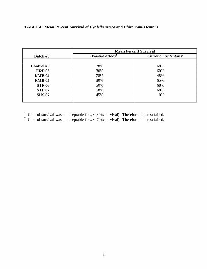
8

TABLE 4. Mean Percent Survival of Hyalella azteca and Chironomus tentans

Mean Percent SurvivalBatch #5 Hyalella azteca1 Chironomus tentans2

Control #5 78% 68%ERP 03 80% 60%

KMB 04 78% 48%KMB 05 80% 65%

STP 06 50% 68%STP 07 68% 68%SUS 07 45% 0%

1 Control survival was unacceptable (i.e., < 80% survival). Therefore, this test failed.2 Control survival was unacceptable (i.e., < 70% survival). Therefore, this test failed.

ACUTE TOXICITY TESTSWITH

HYALELLA AZTECA AND CHIRONOMUS TENTANSON SEDIMENTS FROM THE DULUTH/SUPERIOR HARBOR:

1994 Sampling Results - Batch # 6

Conducted by

Minnesota Pollution Control AgencyMonitoring and Assessment Section

520 Lafayette RoadSt. Paul, Minnesota 55155-4194

April 1997

ii

TABLE OF CONTENTS

INTRODUCTION . . . . . . . . . . . . . . . . . . . . . . . . . . . . . . . . . . . . . . . . . . . . . . . . . . . . . . . . . . . . 1

SAMPLE COLLECTION AND HANDLING . . . . . . . . . . . . . . . . . . . . . . . . . . . . . . . . . . . . . . 1

METHODS . . . . . . . . . . . . . . . . . . . . . . . . . . . . . . . . . . . . . . . . . . . . . . . . . . . . . . . . . . . . . . . . . 1

RESULTS . . . . . . . . . . . . . . . . . . . . . . . . . . . . . . . . . . . . . . . . . . . . . . . . . . . . . . . . . . . . . . . . . . 2

SUMMARY . . . . . . . . . . . . . . . . . . . . . . . . . . . . . . . . . . . . . . . . . . . . . . . . . . . . . . . . . . . . . . . . 4

REFERENCES . . . . . . . . . . . . . . . . . . . . . . . . . . . . . . . . . . . . . . . . . . . . . . . . . . . . . . . . . . . . . . . 4

APPENDIX A - TOXSTAT Analysis

APPENDIX B - Reference Toxicant Control Chart for Hyalella azteca

iii

LIST OF TABLES

TABLE 1. Daily Overlying Water pH Measurements ..................................................................5

TABLE 2. Daily Overlying Water Dissolved Oxygen Concentrations (mg/L)............................. 6

TABLE 3. Daily Overlying Water Temperatures (Degrees Celsius) ........................................... 7

TABLE 4. Mean Percent Survival of Hyalella azteca and Chironomus tentans .......................... 8

1

INTRODUCTION

As part of a sediment assessment of hotspot areas in the Duluth/Superior Harbor, sedimenttoxicity tests were conducted to assess acute (survival) and chronic (growth) toxicity to benthicinvertebrates. Acute effects were measured in separate 10-day toxicity tests to Hyalella azteca(H. azteca) and Chironomus tentans (C. tentans). Growth was measured at the end of theC. tentans test to assess chronic effects. Survival and growth endpoints were compared toorganisms similarly exposed to a reference control sediment collected from West Bearskin Lake(Cook County, MN).

A total of 44 sediment samples were collected for toxicity testing. This report presents theresults of three of these sediment samples.

SAMPLE COLLECTION AND HANDLING

On September 29, 1994 and October 4, 1994, Minnesota Pollution Control Agency (MPCA) staffcollected the three sediments referred to in this report. The samples were collected from theharbor using a gravity corer. The samples were stored at 4°C at the Duluth MPCA office untilthey were transported to the MPCA Toxicology Laboratory in St. Paul, MN.

METHODS

Three sediment samples and a control sediment were subjected to the 10-day sediment toxicitytest using the procedures described in U.S. EPA (1994). The test organisms (H. azteca andC. tentans) were exposed to sediment samples in a portable mini-flow system described in Benoitet al. (1993) and U.S. EPA (1994). The test apparatus consists of 300 mL, glass-beaker testchambers held in a glass box supplied with water from an acrylic plastic headbox. The beakershave two, 1.5 cm holes covered with stainless steel mesh, to allow for water exchange whilecontaining the test organisms. The headbox has a pipette tip drain calibrated to deliver water atan average rate of 32.5 mL/min. The glass box is fitted with a self-starting siphon to provideexchange of overlying water.

The H. azteca used for this test were 1 to 3 mm long, and the C. tentans were approximately 14days old. These organisms were supplied by Environmental Consulting and Testing (Superior,WI) prior to the test set up.

On December 6, 1994, three samples (ERP 01, ERP 02, and STP 03) and the control sedimentwere separately homogenized by hand, and 100 mL of each sediment was placed in a test beaker(Batch #6). Approximately 100 mL of aerated, artesian well water was added to each beaker, andthe sediments were allowed to settle for approximately two hours before the organisms wereadded. For each sediment, nine H. azteca were placed in each of four beakers in a randomfashion, and ten C. tentans were placed randomly in another four beakers. An insufficientnumber of H. azteca organisms were received from the supplier to seed each beaker with tenorganisms.

2

The organisms were exposed to 16 hours of light and eight hours of darkness for the duration ofthe ten-day test. Each day, two liters of aerated water from the artesian well at Stroh Brewery inSt. Paul, MN were exchanged in each test chamber. On weekdays, 1-L was exchanged in themorning and 1-L in the afternoon. On weekends, the two liters were passed through thechambers all at once. Water quality measurements (i.e., pH, temperature, and dissolved oxygen)of the overlying water were taken in one beaker of each of the quadruplicate sets of each of thesediments. The results, along with daily observations involving the physical appearance of thesediments and organisms, were recorded in a laboratory notebook. This notebook is retained onfile at the MPCA.

The test was terminated on December 16, 1994. The sediments were sieved through 40 meshscreens, and the sieved material was sorted for organisms. The organisms found were counted,and the number of alive and dead organisms were recorded. Organisms not found were recordedas missing and presumed dead. The C. tentans that survived were placed in aluminum weighingdishes, dried at approximately 100°C for at least four hours, desiccated to room temperature, andweighed.

Growth (weight) of the C. tentans and survival of both organisms were used as the endpoints forthese tests. The survival data were analyzed using TOXSTAT (Gulley and WEST, Inc., 1994), astatistical software package obtained from the University of Wyoming. However, due to aquality assurance problem, the growth data were not analyzed.

A 96-hour, reference toxicant test with H. azteca in sodium chloride (NaCl) was run inconjunction with these toxicity tests to determine the acceptability of the H. azteca used. Fourconcentrations of NaCl solution (i.e., 10, 5, 2.5, and 1.25 g/L) and a control (aerated, artesianwell water) were used in this test. Three replicates of five organisms each were set up perconcentration.

RESULTS

Water Quality

Measurements of pH, dissolved oxygen, and temperature in the overlying water of the testbeakers were made daily. These measurements are summarized below and in Tables 1, 2, and 3,respectively.

The range of pH values in the beakers containing H. azteca was 7.6 to 8.1 (Table 1). The waterin the C. tentans beakers had a pH range of 7.5 to 7.9 (Table 1). The pH fluctuations duringthese tests were acceptable since they did not vary more than 50% within each treatment(U.S. EPA, 1994).

The dissolved oxygen concentration ranged from 3.6 to 7.4 mg/L in the H. azteca beakers andfrom 3.0 to 7.0 mg/L in the C. tentans beakers (Table 2). It should be noted that on Days 8 and9, the dissolved oxygen concentration in the STP 3 sediment beaker containing C. tentans was

3

less than 40% saturated, which is out of the acceptable test range for dissolved oxygen. Theorganisms continued to be fed throughout the test.

The temperature of the overlying water in each glass box was measured and ranged from 19.5°Cto 21.5°C in the H. azteca beakers and from 19.5°C to 21.0°C in the C. tentans beakers (Table 3).The recommended temperature for these tests is 23 ± 1°C (U.S. EPA, 1994).

Test Endpoints

Survival Data

The mean percent survival of the test organisms is summarized below and in Table 4.

The mean percent survival of H. azteca in the control was 92% with a range of 89% to 100%. Forthe control sediment containing C. tentans, percent survival ranged from 70% to 90% with amean of 85%. Survival for these controls was acceptable, and both tests passed.

Mean percent survival of H. azteca in the test sediments ranged from 58% in the ERP 02sediment to 80% in the STP 03 sediment. Mean percent survival of C. tentans in the testsediments ranged from 62% in the STP 03 sample to 90% in the ERP 02 sample.

C. Tentans Growth Data

Although the dried C. tentans were weighed, the balance on which they were weighed was notcalibrated with standard weights. Therefore, the data are suspect since the internal calibration ofthe balance may have drifted with time. Thus, no conclusions can be made regarding chronictoxicity (growth).

Data Analysis

All survival data were transformed using an arc sine-square root transformation. A one-tailedstatistical test was used to test the alternative hypothesis that sample survival was less thancontrol survival. For H. azteca, a nonparametric statistical test (i.e., Steel’s Many-one Rank test)had to be used due to non-normal data. Only the survival of H. azteca in the ERP 02 sedimentwas significantly less than the control (α = 0.05). For C. tentans, Dunnett’s test was used todetermine that none of the test sediments were toxic compared to the control sediment (p = 0.05).Results of the statistical analyses of these data are included in Appendix A.

Reference Toxicant Test with Hyalella azteca in Sodium Chloride Solution

The pH of the overlying water in the reference toxicant test ranged from 8.1 to 8.7. Thedissolved oxygen ranged from 7.5 to 8.3 mg/L, and the temperature of the overlying water rangedfrom 20.0°C to 22.0°C. Survival of the organisms in the control was greater than 90% (i.e.,100%) which was acceptable.

4

The LC50 for this reference toxicant test was 4.45 g/L NaCl as determined by the TrimmedSpearman-Karber method and was within plus or minus two standard deviations of the runningmean (Appendix B). The running mean for this test, which was 3.82 ± 1.14 g/L with a CV of30%, was based on the previous five acceptable reference toxicant tests performed by thislaboratory.

SUMMARY

Survival of H. azteca in the control sediment was acceptable (i.e., greater than 80%). Survival ofthe H. azteca in the reference toxicant test was also acceptable (i.e., greater than 90%). Survivalof the H. azteca in the ERP 02 sediment was significantly less than the corresponding controlsurvival (α = 0.05).

Control survival was acceptable in the C. tentans test (i.e., greater than 70%), and there was nostatistically significant difference between survival of the C. tentans in any of the test sedimentswith the control sediment.

REFERENCES

Benoit, D.A., G. Phipps, and G.T. Ankley. 1993. A sediment testing intermittent renewal system for the automated renewal of overlying water in toxicity tests with contaminated sediments. Water Research 27:1403-1412.

Gulley, D.D. and WEST, Inc. 1994. TOXSTAT 3.4. WEST, Inc., Cheyenne, WY.

U.S. EPA. 1994. Methods for measuring the toxicity and bioaccumulation of sediment-associated contaminants with freshwater invertebrates. Office of Research and Development, U.S. Environmental Protection Agency, Duluth, MN. EPA/600/R-94/024.

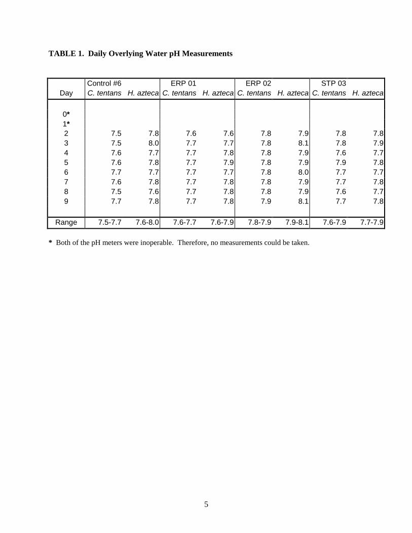
5

TABLE 1. Daily Overlying Water pH Measurements

Control #6 ERP 01 ERP 02 STP 03Day C. tentans H. azteca C. tentans H. azteca C. tentans H. azteca C. tentans H. azteca

0*1*2 7.5 7.8 7.6 7.6 7.8 7.9 7.8 7.83 7.5 8.0 7.7 7.7 7.8 8.1 7.8 7.94 7.6 7.7 7.7 7.8 7.8 7.9 7.6 7.75 7.6 7.8 7.7 7.9 7.8 7.9 7.9 7.86 7.7 7.7 7.7 7.7 7.8 8.0 7.7 7.77 7.6 7.8 7.7 7.8 7.8 7.9 7.7 7.88 7.5 7.6 7.7 7.8 7.8 7.9 7.6 7.79 7.7 7.8 7.7 7.8 7.9 8.1 7.7 7.8

Range 7.5-7.7 7.6-8.0 7.6-7.7 7.6-7.9 7.8-7.9 7.9-8.1 7.6-7.9 7.7-7.9

* Both of the pH meters were inoperable. Therefore, no measurements could be taken.

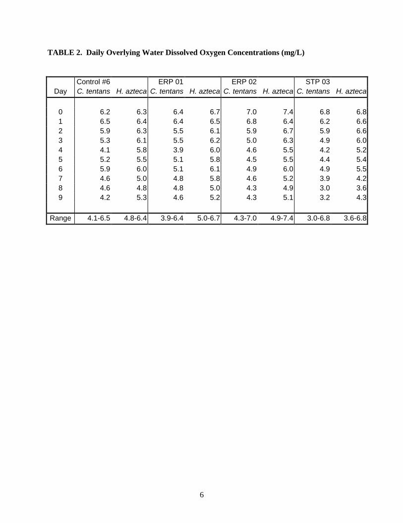
6

TABLE 2. Daily Overlying Water Dissolved Oxygen Concentrations (mg/L)

Control #6 ERP 01 ERP 02 STP 03Day C. tentans H. azteca C. tentans H. azteca C. tentans H. azteca C. tentans H. azteca

0 6.2 6.3 6.4 6.7 7.0 7.4 6.8 6.81 6.5 6.4 6.4 6.5 6.8 6.4 6.2 6.62 5.9 6.3 5.5 6.1 5.9 6.7 5.9 6.63 5.3 6.1 5.5 6.2 5.0 6.3 4.9 6.04 4.1 5.8 3.9 6.0 4.6 5.5 4.2 5.25 5.2 5.5 5.1 5.8 4.5 5.5 4.4 5.46 5.9 6.0 5.1 6.1 4.9 6.0 4.9 5.57 4.6 5.0 4.8 5.8 4.6 5.2 3.9 4.28 4.6 4.8 4.8 5.0 4.3 4.9 3.0 3.69 4.2 5.3 4.6 5.2 4.3 5.1 3.2 4.3

Range 4.1-6.5 4.8-6.4 3.9-6.4 5.0-6.7 4.3-7.0 4.9-7.4 3.0-6.8 3.6-6.8

7

TABLE 3. Daily Overlying Water Temperatures (Degrees Celsius)

Control #6 ERP 01 ERP 02 STP 03Day C. tentans H. azteca C. tentans H. azteca C. tentans H. azteca C. tentans H. azteca

0 19.5 19.5 19.5 19.5 19.5 19.5 19.5 19.51 20.4 20.4 20.6 20.6 20.4 20.4 21.0 21.02 20.0 20.0 20.5 20.5 20.2 20.2 21.0 21.03 20.0 20.0 20.5 20.5 20.0 20.0 19.5 19.54 20.5 20.5 20.5 20.5 20.5 20.5 21.0 21.55 20.5 20.5 20.5 20.5 20.5 20.5 20.5 20.56 20.2 20.2 20.5 20.5 20.5 20.5 21.0 21.07 20.2 20.2 20.5 20.5 20.2 20.2 21.0 21.08 20.0 20.0 20.5 20.5 20.0 20.0 21.0 21.09 20.2 20.2 20.8 20.8 20.4 20.4 21.0 21.0

Range 19.5-20.5 19.5-20.5 19.5-20.8 19.5-20.8 19.5-20.5 19.5-20.5 19.5-21.0 19.5-21.5

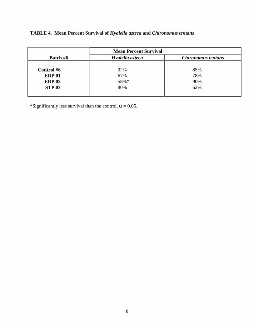
8

TABLE 4. Mean Percent Survival of Hyalella azteca and Chironomus tentans

Mean Percent SurvivalBatch #6 Hyalella azteca Chironomus tentans

Control #6 92% 85%ERP 01 67% 78%ERP 02 58%* 90%STP 03 80% 62%

*Significantly less survival than the control, α = 0.05.

APPENDIX A

TOXSTAT Analysis

A-1

94MUDPUPPY RUN #6 HYALELLA 12/6/9444444

CONTROL0.891.000.890.89

ERP 10.110.890.890.78

ERP 20.560.440.670.67

STP 30.780.890.670.89

A-2

TITLE: 94MUDPUPPY RUN #6 HYALELLA 12/6/94FILE: S:\MA\CHUBBAR\TSD\94MUD\94MPR6H.DATTRANSFORM: ARC SINE(SQUARE ROOT(Y)) NUMBER OF GROUPS: 4--------------------------------------------------------------------

GRP IDENTIFICATION REP VALUE TRANS VALUE--- ---------------- ---- ------------- -------------1 CONTROL 1 0.8900 1.23271 CONTROL 2 1.0000 1.40341 CONTROL 3 0.8900 1.23271 CONTROL 4 0.8900 1.23272 ERP 1 1 0.1100 0.33812 ERP 1 2 0.8900 1.23272 ERP 1 3 0.8900 1.23272 ERP 1 4 0.7800 1.08263 ERP 2 1 0.5600 0.84553 ERP 2 2 0.4400 0.72533 ERP 2 3 0.6700 0.95893 ERP 2 4 0.6700 0.95894 STP 3 1 0.7800 1.08264 STP 3 2 0.8900 1.23274 STP 3 3 0.6700 0.95894 STP 3 4 0.8900 1.2327--------------------------------------------------------------------

A-3

94MUDPUPPY RUN #6 HYALELLA 12/6/94File: S:\MA\CHUBBAR\TSD\94MUD\94MPR6H.DATTransform: ARC SINE(SQUARE ROOT(Y))

Shapiro - Wilk's test for normality----------------------------------------------------------------------

D = 0.662

W = 0.826

Critical W (P = 0.05) (n = 16) = 0.887Critical W (P = 0.01) (n = 16) = 0.844----------------------------------------------------------------------

Data FAIL normality test. Try another transformation.

Warning - The first three homogeneity tests are sensitive to non-normal

data and should not be performed.

94MUDPUPPY RUN #6 HYALELLA 12/6/94File: S:\MA\CHUBBAR\TSD\94MUD\94MPR6H.DATTransform: ARC SINE(SQUARE ROOT(Y))

----------------------------------------------------------------------Bartlett's test for homogeneity of varianceCalculated B1 statistic = 9.11

----------------------------------------------------------------------Table Chi-square value = 11.34 (alpha = 0.01, df = 3)Table Chi-square value = 7.81 (alpha = 0.05, df = 3)

Data PASS B1 homogeneity test at 0.01 level. Continue analysis.

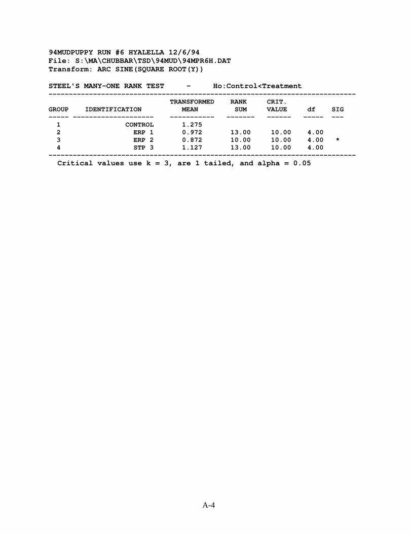
A-4

94MUDPUPPY RUN #6 HYALELLA 12/6/94File: S:\MA\CHUBBAR\TSD\94MUD\94MPR6H.DATTransform: ARC SINE(SQUARE ROOT(Y))

STEEL'S MANY-ONE RANK TEST - Ho:Control<Treatment----------------------------------------------------------------------------

TRANSFORMED RANK CRIT.GROUP IDENTIFICATION MEAN SUM VALUE df SIG----- -------------------- ----------- ------- ------ ----- ---

1 CONTROL 1.2752 ERP 1 0.972 13.00 10.00 4.003 ERP 2 0.872 10.00 10.00 4.00 *4 STP 3 1.127 13.00 10.00 4.00

----------------------------------------------------------------------------Critical values use k = 3, are 1 tailed, and alpha = 0.05

A-5

94 MUDPUPPY RUN #6 CHIRONOMIDS 12/6/9444444

CONTROL0.90.90.70.9

ERP 11.00.80.70.6

ERP 21.00.80.90.9

STP 30.80.50.70.5

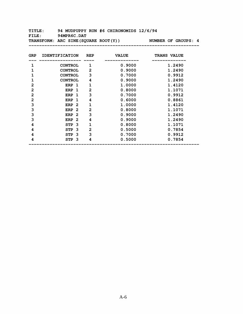
A-6

TITLE: 94 MUDPUPPY RUN #6 CHIRONOMIDS 12/6/94FILE: 94MPR6C.DATTRANSFORM: ARC SINE(SQUARE ROOT(Y)) NUMBER OF GROUPS: 4-----------------------------------------------------------------

GRP IDENTIFICATION REP VALUE TRANS VALUE--- ---------------- ---- ------------- -------------1 CONTROL 1 0.9000 1.24901 CONTROL 2 0.9000 1.24901 CONTROL 3 0.7000 0.99121 CONTROL 4 0.9000 1.24902 ERP 1 1 1.0000 1.41202 ERP 1 2 0.8000 1.10712 ERP 1 3 0.7000 0.99122 ERP 1 4 0.6000 0.88613 ERP 2 1 1.0000 1.41203 ERP 2 2 0.8000 1.10713 ERP 2 3 0.9000 1.24903 ERP 2 4 0.9000 1.24904 STP 3 1 0.8000 1.10714 STP 3 2 0.5000 0.78544 STP 3 3 0.7000 0.99124 STP 3 4 0.5000 0.7854-----------------------------------------------------------------

A-7

94 MUDPUPPY RUN #6 CHIRONOMIDS 12/6/94File: 94MPR6C.DAT Transform: ARC SINE(SQUARE ROOT(Y))

Shapiro - Wilk's test for normality----------------------------------------------------------------------

D = 0.328

W = 0.953

Critical W (P = 0.05) (n = 16) = 0.887Critical W (P = 0.01) (n = 16) = 0.844----------------------------------------------------------------------

Data PASS normality test at P=0.01 level. Continue analysis.

94 MUDPUPPY RUN #6 CHIRONOMIDS 12/6/94File: 94MPR6C.DAT Transform: ARC SINE(SQUARE ROOT(Y))

----------------------------------------------------------------------Bartlett's test for homogeneity of varianceCalculated B1 statistic = 1.30

----------------------------------------------------------------------Table Chi-square value = 11.34 (alpha = 0.01, df = 3)Table Chi-square value = 7.81 (alpha = 0.05, df = 3)

Data PASS B1 homogeneity test at 0.01 level. Continue analysis.

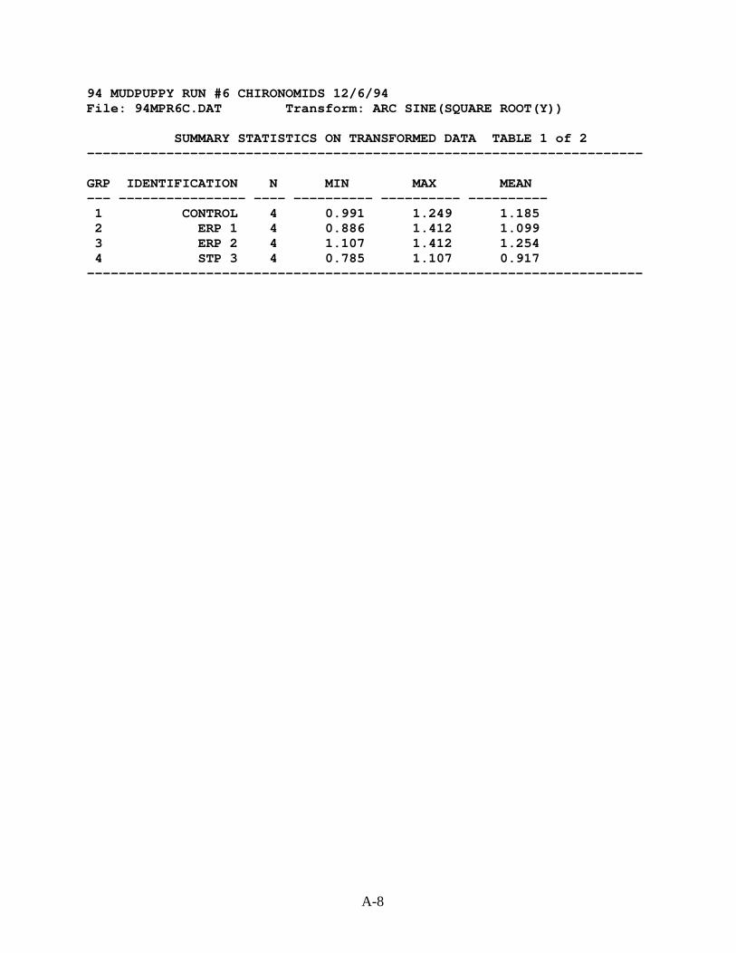
A-8

94 MUDPUPPY RUN #6 CHIRONOMIDS 12/6/94File: 94MPR6C.DAT Transform: ARC SINE(SQUARE ROOT(Y))

SUMMARY STATISTICS ON TRANSFORMED DATA TABLE 1 of 2----------------------------------------------------------------------

GRP IDENTIFICATION N MIN MAX MEAN--- ---------------- ---- ---------- ---------- ----------1 CONTROL 4 0.991 1.249 1.1852 ERP 1 4 0.886 1.412 1.0993 ERP 2 4 1.107 1.412 1.2544 STP 3 4 0.785 1.107 0.917----------------------------------------------------------------------

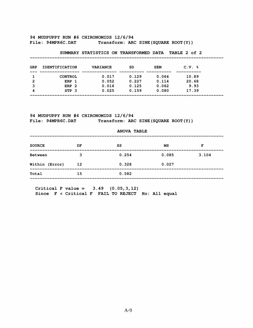
A-9

94 MUDPUPPY RUN #6 CHIRONOMIDS 12/6/94File: 94MPR6C.DAT Transform: ARC SINE(SQUARE ROOT(Y))

SUMMARY STATISTICS ON TRANSFORMED DATA TABLE 2 of 2------------------------------------------------------------------------------

GRP IDENTIFICATION VARIANCE SD SEM C.V. %--- ---------------- -------------- ---------- ---------- ----------1 CONTROL 0.017 0.129 0.064 10.892 ERP 1 0.052 0.227 0.114 20.683 ERP 2 0.016 0.125 0.062 9.934 STP 3 0.025 0.159 0.080 17.39

------------------------------------------------------------------------------

94 MUDPUPPY RUN #6 CHIRONOMIDS 12/6/94File: 94MPR6C.DAT Transform: ARC SINE(SQUARE ROOT(Y))

ANOVA TABLE------------------------------------------------------------------------------

SOURCE DF SS MS F------------------------------------------------------------------------------Between 3 0.254 0.085 3.104

Within (Error) 12 0.328 0.027------------------------------------------------------------------------------Total 15 0.582------------------------------------------------------------------------------

Critical F value = 3.49 (0.05,3,12)Since F < Critical F FAIL TO REJECT Ho: All equal

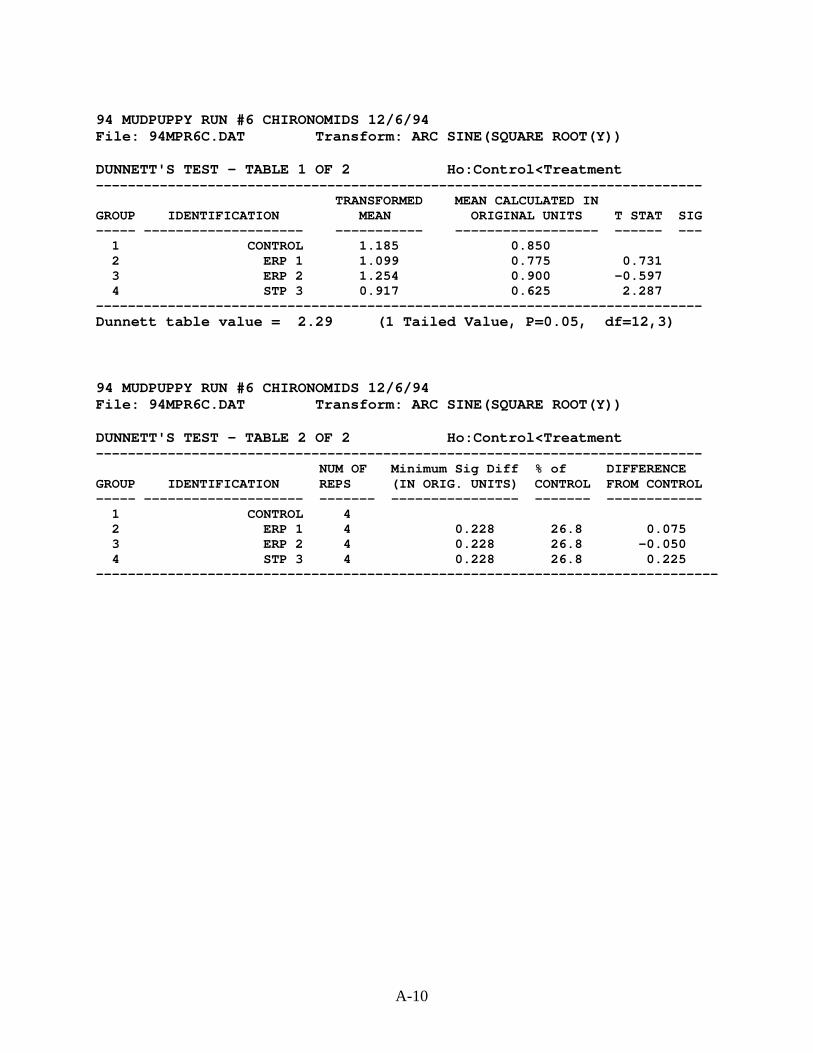
A-10

94 MUDPUPPY RUN #6 CHIRONOMIDS 12/6/94File: 94MPR6C.DAT Transform: ARC SINE(SQUARE ROOT(Y))

DUNNETT'S TEST - TABLE 1 OF 2 Ho:Control<Treatment----------------------------------------------------------------------------

TRANSFORMED MEAN CALCULATED INGROUP IDENTIFICATION MEAN ORIGINAL UNITS T STAT SIG----- -------------------- ----------- ------------------ ------ ---

1 CONTROL 1.185 0.8502 ERP 1 1.099 0.775 0.7313 ERP 2 1.254 0.900 -0.5974 STP 3 0.917 0.625 2.287

----------------------------------------------------------------------------Dunnett table value = 2.29 (1 Tailed Value, P=0.05, df=12,3)

94 MUDPUPPY RUN #6 CHIRONOMIDS 12/6/94File: 94MPR6C.DAT Transform: ARC SINE(SQUARE ROOT(Y))

DUNNETT'S TEST - TABLE 2 OF 2 Ho:Control<Treatment----------------------------------------------------------------------------

NUM OF Minimum Sig Diff % of DIFFERENCEGROUP IDENTIFICATION REPS (IN ORIG. UNITS) CONTROL FROM CONTROL----- -------------------- ------- ---------------- ------- ------------

1 CONTROL 42 ERP 1 4 0.228 26.8 0.0753 ERP 2 4 0.228 26.8 -0.0504 STP 3 4 0.228 26.8 0.225

------------------------------------------------------------------------------

APPENDIX B

Reference Toxicant Control Chartfor Hyalella azteca

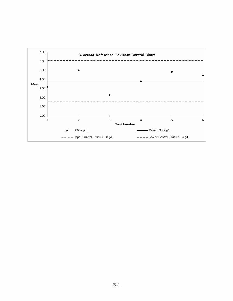
B-1

H. azteca Reference Toxicant Control Chart

0.00

1.00

2.00

3.00

4.00

5.00

6.00

7.00

1 2 3 4 5 6Test Number

LC50

LC50 (g/L) Mean = 3.82 g/L

Upper Control Limit = 6.10 g/L Low er Control Limit = 1.54 g/L

APPENDIX C

BENTHOLOGICAL COMMUNITY DATA

C-1

APPENDIX C

BENTHIC MACROINVERTEBRATE DATA FILES

The below data files contain the benthological abundance and taxa richness data. Due to thelarge size of these files, each site file is split into an oligochaete and insect data file. All files arein Lotus 1-2-3, version 2.3, and are provided on the computer disk at the back of this report.Since all of the files are compressed, access the Readme.txt file first for directions on how toread the files.

DMIR Sites SUS Sitesdmirinse.wk1 susinsec.wk1

susoligo.wk1dmirolig.wk1

WLS SitesERP Sites wlsinse1.wk1

erpinsec.wk1 wlsinse2.wk1erpoligo.wk1 wlsolig1.wk1

wlsolig2.wk1HOB Sites

hobinse1.wk1hobinse2.wk1hobolig1.wk1hobolig2.wk1

KMB Siteskmbinsec.wk1kmboligo.wk1

MLH Sitesmlhinsec.wk1mlholigo.wk1

MNS Sitesmnsinsec.wk1mnsoligo.wk1

STP Sitesstpinsec.wk1stpoligo.wk1