sector news sentiment indices - …€¦ · the gics classification covers 11 sectors, 24 industry...

REU

TER

S/Br

ian

Snyd

er

Sector News Sentiment IndicesDr. Svetlana Borovkova, Associate Professor, Vrije Universiteit Amsterdam, and Head of Quantitative Modelling, Probability and Partners; Philip Lammers, Researcher, Vrije Universiteit Amsterdam, and Investment Analyst, Quantrust Asset Management

Sector News Sentiment Indices 2

We present the sector-based news sentiment indices, which track, for a given industry or sector, the current media sentiment about this sector. The sentiment index for a particular sector has a natural relationship to the basket of stocks of publicly traded companies operating in this sector or the corresponding sector’s ETF. We empirically investigate this relationship for 11 sectors and show that this relationship is particularly signicant at times of market downturns. We demonstrate the added value of such sentiment indices in sector-rotation investment strategies.

Introduction

Academics and finance professionals have been long fascinated by the relationships between news and asset prices. At first, studies on this subject predominantly covered scheduled company announcements. Nowadays, with the emergence of natural language processing algorithms, the focus shifted towards investigating the influence of the sentiment in unscheduled news and social media (such as Twitter messages) on stock and commodity returns.

Most such studies focus on individual stocks and investigate how news about a specific company influences a company’s stock price. However, in many cases, a number of companies from the same industry or even an entire industry is mentioned in a news article. This generates the sentiment in the financial marketplace about an industry or a sector as a whole, rather than related to one specific stock. In this paper, we capture exactly this kind of sentiment.

Our previous paper (Borovkova et al. (2016)) investigated the role of news sentiment in the domain of systemic risk, i.e., the risk associated with the entire financial system. The news sentiment for systemically important financial institutions was used there to measure financial distress. That paper revealed the impressive power of using news sentiment to monitor and even forecast stress in the global financial system. It was found that the news-based systemic risk measure SenSR signals an increase in the financial distress up to 12 weeks before other risk measures do so. Here, we extend SenSR methodology to sectors other than financials and develop similar sentiment measures for other sectors.

In this paper, the news sentiment is tracked on the sector level, which so far has been largely ignored by the literature. We are particularly interested in investigating the relationships between sector news sentiment and aggregated stock prices in that sector, and using these relationships to devise trading and investment strategies (commonly referred to as sector rotation strategies), that are superior to those that do not use sentiment.


Methodology

To define the sectors that we consider and the stock universe corresponding to each sector, we use the constituents of sector-specific Exchange Traded Funds (ETF). We present our analysis for the U.S. stock market; for other regions, the methodology is the same and only the stock universe is different. Sectors are defined on the basis of the Global Industry Classification Standard (GICS), which is a ”pyramid” representing different business sectors. At the top level of the pyramid are the “Sectors,” the second level defines the ”Industry Groups,” the third the ”Industries” and the fourth the ”Sub Industries.” The GICS classification covers 11 sectors, 24 industry groups, 68 industries and 157 sub-industries. In this paper, we only use sectors; however, more detailed and specific news indicators (e.g., corresponding to industries) can be defined in the same way.

Table 1: Summary of sectors, stocks and number of news items from 2003 to 2017

Sector Number of Companies

Number of Items Avg News per Company Ratio

Gini-Coecient Skewness

Financials 44 421.026 9569 0.51 2.01

Consumer Discretionary

42 258.265 6149 0.49 4.31

Energy 42 255.203 6076 0.39 2.62

Consumer Staples 28 141.469 5052 0.45 2.72

Industrials 74 337.867 4566 0.53 3.87

Telecom 21 90.887 4328 0.71 2.3

Materials 33 136.079 4124 0.41 1.32

Information Technology

136 440.695 3240 0.54 4.34

Health Care 118 357.975 3034 0.52 3.03

Utilities 52 151.435 2912 0.41 1.11

Real Estate 121 193.823 1602 0.34 0.96

Σ 711 2.784.724 3917 - -

Table 1 summarizes the data that we use: In total, we include 711 stocks, for which a total of 2,784,724 news items were available in the period 2003-2017. The largest sector (in terms of both the number of stocks and news) is information technology and the smallest sector is telecom. In relative terms (the ratio between news items and companies per sector), financials is the best covered sector, with an average of 9,569 news items per company, which is three times more than the average – this undoubtedly has something to do with the financial crisis and media attention it attracted. In terms of dispersion, we see that the news flow is heavily tilted (probably towards larger companies), as we find positive skewness in the news distribution and high Gini coefficients (recall that Gini coefficient measures the degree of dispersion, or ”inequality”: In our case, the coefficient of 1 would indicate that all news is about just one company and a value of 0 would indicate that news items are perfectly equally spread over all companies). This could be a result of big corporates receiving more attention by analysts and media in general.

The source of the sentiment data is the Thomson Reuters News Analytics engine (TRNA). This engine, based on complex natural language processing algorithms, ”reads” and interprets (in real time) all news that reaches the Thomson Reuters newswire. Each news item is tagged in relation to a company or a commodity – currently 37,000 companies worldwide are incorporated into the engine, as well as 40 commodity classes. The alg rithms return, for each news item, a wealth of quantitative characteristics, the most important being the sentiment score. The relevance score is provided too, indicating how relevant a particular news item is for that asset. Furthermore, a variety of novelty indicators are given, such as a number of similar news items that have been identified before and after that particular news item.

The outputs of the TRNA engine, which we directly use in this paper, are summarized below:

• Relevance: A score between 0 and 1, which indicates the likelihood of a news item being relevant for a specific company or commodity.

• Sentiment Score: Expresses the likelihood that a particular news item conveys positive, negative or neutral outlook with regard to the relevant asset.

• Novelty: A number which counts how many news items with similar content were published in the past. The database covers different time spans: 12 hours, 24 hours, 3 days, 5 days and 1 week.


The raw news sentiment scores for a particular stock are volatile and the news flow is irregular (more frequent for larger stocks, less frequent for smaller stocks). So to put the sentiment in a broader context, it is necessary to clean the news sentiment data, as well as to ”de-noise” it in some way, without removing relevant information. The methodology for this is based on the one developed by us for the sentiment-based systemic risk indicator SenSR, whose description can be found in Borovkova et al. (2016). For completeness, we briefly summarize this methodology here.

For each stock, the sentiment indicator is generated first, by completing the following steps.

First, as in Borovkova and Mahakena (2015) and Borovkova et al. (2016), all less relevant news items are removed: A news item is considered to be irrelevant if the relevance score is smaller than 30% or the absolute difference between positive and negative sentiment is smaller than 5%.

In the next step, the stock-specific sentiment scores are aggregated into weekly sentiment scores, accounting for the relevance and novelty of each news item. This aggregation already removes some noise; however, weekly sentiment scores remain rather volatile. In this paper, the time scale is set to be weekly, but a higher or lower frequency of measuring the sentiment (such as daily or monthly) is possible too, depending on the goal and the application of the sentiment indices. Each news item’s sentiment is weighted according to its relevance and more novel news items get higher weight when sentiments are aggregated.

The next step is filtering of the unobserved sentiment from the observed noisy sentiment scores. This step follows the SenSR methodology closely, utilizing the Kalman filter. The Kalman filter is an econometric method which aims to filter the unobserved ”state” of a system from observed noisy data. Thus, we assume that there is some underlying level of sentiment, which we observe with noise and which we estimate using this method.

Following Borovkova and Mahakena (2015) and Borovkova et al. (2016), it is assumed that we have an unobserved sentiment – the state variable µt, and the observed signal yt. The Local News Sentiment Level (LNSL) model is defined as

The equations (1) and (2) are used to extract the unobserved sentiment from the weekly sentiment scores by means of the Kalman filter.

To illustrate the difference between the unfiltered and filtered sentiments, Figures 1a and 1b present the positive, neutral and negative news sentiment for eBay, before and after the filtering, based on the weekly data. From these figures we can see how filtering removes the noise and clear sentiment trends emerge.

Figure 1: Comparison between weekly unfiltered and weekly filtered sentiment

(a) Weekly raw sentiment data for eBay. Green represents positive, red negative and black neutral sentiment

(b) Weekly Kalman-filtered sentiment data for eBay. Green represents positive, red negative and black neutral sentiment


The final step in generating sector-specific news sentiment indicators is aggregation of filtered sentiments among stocks in a specific sector. The approach here is different to Borovkova et al. (2016), as we do not weigh companies by their debt or leverage (which is appropriate for financial institutions, but not for other companies), but use either market cap or equal weights. We use the weekly scaled net positive sentiment, defined as

where pk,t is the sentiment score for the k-th company at time t. The sentiment index for a particular sector i (which we call SINS, for Sector and INdustry Sentiment) is then defined as

where Ni is the number of companies we include to represent the sector i. Here wk,t is the weight assigned to company k at time t (either market cap-based weights or equal weights 1/Ni) and M M is the moving median calculated over a period of the last five years.

Note that the sector sentiment index SINS is scaled with respect to its moving median. This scaling allows us to make judgment about the current sentiment relative to its past values, as a sentiment score above 100 indicates a higher sentiment than in 50% of the past five years and a score below 100 indicates worse sentiment than in 50% of the past time period. The time period for calculating the moving median is set to five years; however, other choices are possible, as the results are quite robust to the choice of the moving window.


Empirical analysis of the sector sentiment indices

Here we present the results for a number of the 11 investigated sectors; most of the common observations or patterns found across sectors are discussed below. The graphical illustrations for the remaining sectors can be found in the Appendix.

We start with showing the historical sentiment indices, from 2005 until 2017. These are shown in Figure 2.

Figure 2: Sentiment indices for eight sectors

Now we show some of the sentiment indices together with the price development of the corresponding basket of stocks (figures for sectors not shown are in the Appendix). For the U.S. energy sector, this is shown in Figure 3. It can be seen how the energy sector sentiment collapsed following the decline in oil price observed from June 2014 (which was caused by the increase in the U.S. domestic shale oil production). During this time period, the net sentiment became negative, which is a unique feature across all sectors. Generally, the energy sector sentiment is very volatile, compared to other sectors. It is also interesting to see that lower oil prices seen in recent years impact this sector’s sentiment more than the financial crisis of 2008. This indicates that the information captured by the sector sentiment is mostly sector-specific. There are certainly some co-movements between the sentiment and price indices (in fact, it can be shown that the two series are co-integrated), but it appears that the sentiment also captures other information than that reflected in the price development.

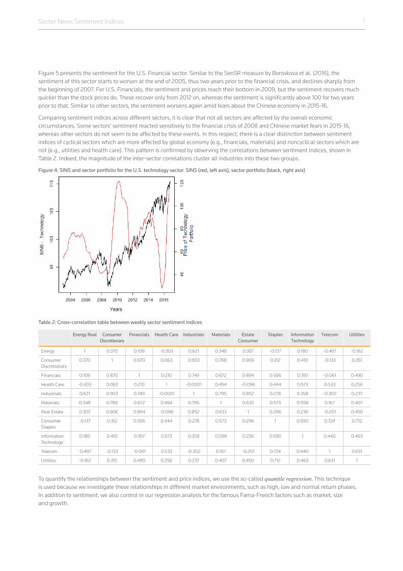
The sentiment index for the technology sector is shown in Figure 4. Tech sector sentiment is much less volatile (see the left axis) and always positive. It is notable that there is no significant impact of the financial crisis of 2008. In the post-crisis period, sentiment increases very fast and reaches its peak in the beginning of 2010. The stock prices for tech stocks do not share this pattern, as prices continue to rise while the sentiment is declining. At the end of 2015, the sentiment index reaches its minimum. The reason for that is likely the fear of a possible collapse of the Chinese economy, prevalent at that time. After that, the tech sentiment shows a sharp increase in 2016, which also coincides with the 13 % return seen in that year.

Figure 3: SINS (sector sentiment) and sector stock portfolio for the U.S. Energy Sector. SINS (red, left axis), sector portfolio (black, right axis)


Figure 5 presents the sentiment for the U.S. Financial sector. Similar to the SenSR measure by Borovkova et al. (2016), the sentiment of this sector starts to worsen at the end of 2005, thus two years prior to the financial crisis, and declines sharply from the beginning of 2007. For U.S. Financials, the sentiment and prices reach their bottom in 2009, but the sentiment recovers much quicker than the stock prices do. These recover only from 2012 on, whereas the sentiment is significantly above 100 for two years prior to that. Similar to other sectors, the sentiment worsens again amid fears about the Chinese economy in 2015-16.

Comparing sentiment indices across different sectors, it is clear that not all sectors are affected by the overall economic circumstances. Some sectors’ sentiment reacted sensitively to the financial crisis of 2008 and Chinese market fears in 2015-16, whereas other sectors do not seem to be affected by these events. In this respect, there is a clear distinction between sentiment indices of cyclical sectors which are more affected by global economy (e.g., financials, materials) and noncyclical sectors which are not (e.g., utilities and health care). This pattern is confirmed by observing the correlations between sentiment indices, shown in Table 2. Indeed, the magnitude of the inter-sector correlations cluster all industries into these two groups.

Figure 4: SINS and sector portfolio for the U.S. technology sector. SINS (red, left axis), sector portfolio (black, right axis)

Table 2: Cross-correlation table between weekly sector sentiment indices

Energy Real Consumer Discretionary

Financials Health Care Industrials Materials Estate Consumer

Staples Information Technology

Telecom Utilities

Energy 1 0:370 0:109 -0:303 0:621 0:348 0:307 -0:137 0:180 -0:497 -0:162

Consumer Discretionary

0:370 1 0:870 0:063 0:903 0:788 0:906 0:312 0:410 -0:133 0:351

Financials 0:109 0:870 1 0:210 0:749 0:672 0:894 0:306 0:397 -0:061 0:490

Health Care -0:303 0:063 0:210 1 -0:0001 0:494 -0:096 0:444 0:573 0:533 0:256

Industrials 0:621 0:903 0:749 -0:0001 1 0:795 0:852 0:278 0:358 -0:302 0:237

Materials 0:348 0:788 0:672 0:494 0:795 1 0:633 0:573 0:598 0:167 0:407

Real Estate 0:307 0:906 0:894 -0:096 0:852 0:633 1 0:296 0:236 -0:201 0:450

Consumer Staples

-0:137 0:312 0:306 0:444 0:278 0:573 0:296 1 0:590 0:724 0:712

Information Technology

0:180 0:410 0:397 0:573 0:358 0:598 0:236 0:590 1 0:440 0:463

Telecom -0:497 -0:133 -0:061 0:533 -0:302 0:167 -0:201 0:724 0:440 1 0:631

Utilities -0:162 0:351 0:490 0:256 0:237 0:407 0:450 0:712 0:463 0:631 1

To quantify the relationships between the sentiment and price indices, we use the so-called quantile regression. This technique is used because we investigate these relationships in different market environments, such as high, low and normal return phases. In addition to sentiment, we also control in our regression analysis for the famous Fama-French factors such as market, size and growth.


Figure 5: Development of SINS and sector portfolio for the U.S. financial sector. SINS (red, left axis), sector-portfolio (black, right axis)

Our quantile regression model has the form

where i is the index corresponding to the ith sector and t is time (in weeks). Here r it (τ) is the sector i portfolio return in week t,

which falls into the quantile τ.

The fitted quantile regression models show that the sentiment influence varies significantly between low and high return quantiles, for almost all sectors. Figures 6 and 7 illustrate this for the tech a nd financial sectors. These figures show the coefficients β i

5(τ ) (which measure the influence of the sentiment on the returns), as functions of return’s quantile τ (the solid red line everywhere indicates the overall OLS coefficient estimate).

Figure 6: β5(τ) coefficient of quantile regression for tech sector

Figure 7: β5(τ) coefficients of quantile regression for financials sector


From these figures we can see that, for lower quantiles (low returns), the influence of net sentiment is positive and significant, whereas for higher quantiles (high returns), the situation is reversed: The effect of sentiment is negative (and also significant). For the in-between quantiles, the effects are ambiguous and not significant. This means, first of all, that the impact of news sentiment can be seen only for high (in absolute value) positive or negative returns, but not at ”normal” times. The second observation is that at times of low returns, the effect of sentiment is positive: A rising sentiment is accompanied by higher returns, which is what we would expect. Surprisingly, the opposite pattern is observed in a high returns regime: Declining sentiment is accompanied by higher returns and vice versa.

The explanation of these findings lies in the well-known behavioral biases of investors. For example, the famous confirmation and optimism biases manifest themselves here by a weak or even inverse relationship between sentiment and returns at the times when markets are rising. When returns are negative, the sentiment has strong effect and that is related to the confirmation and self-serving biases.

In general, nearly all sectors show this pattern, even though the magnitude of the effects across sectors is varied. The only exception is the utilities sector, which shows nonsignificant effects of news sentiment for all quantiles. In contrast, the financials sector shows the most significant sentiment effects over the complete range of quantiles.


Using sentiment indices for sector rotation: an illustration

One of our findings is the positive and significant relationship between the sector sentiment and ETF returns in a bullish (i.e., downward) market environment. So we will use this in devising a simple sector rotation strategy which uses, among other things, the sector sentiment as a trading signal. More specifically, we will use the declining sector sentiment as the additional signal to get out of a position in a certain sector, exploring the strong relationship between the declining sentiment and returns. In other words, the sentiment will be used here for identifying ”sell” signals only, thus when to sell a position or when to short the market (if short selling is allowed). We would like to stress that we do not suggest any sophisticated trading strategies here; the strategies we discuss here are very simple and are intended as an illustration of the power of sentiment signals.

We look at two types of investment style: one of an active investment manager and another of a more passive investor. These two types of investors are distinguished by their ability to trade (and hence, their frequency of portfolio rebalancing). We assume that an active manager is able to rebalance his or her portfolio weekly, while a more passive investor rebalances monthly.

We limit the sources of trading signals to two variables: price and sentiment. We generate a trading signal by means of a logit model, estimated on the basis of a rolling window. With this model, the probability of the ETF price going down in the next period (a week or a month) is estimated on the basis of changes in sentiment as well as other possibly relevant variables, such as trading volume and yield spread. If the predicted probability of the price decline is greater than some predetermined threshold (e.g., 0.5), the sell signal is triggered.

In addition to a sell signal obtained from the above logit model, we use the traditional moving average crossover strategy to generate a buy, hold or sell signal in each week. However, we buy or hold on the basis of the moving average-based signal only and we sell on the basis of both the moving average crossover and the sentiment (so the two signals must confirm each other for a sell signal to be triggered). The long moving average is eight weeks, the short one is one week and the difference between the two must be more than 4% to generate a trading signal (so if ETF’s volatility is 17% p/a, this threshold would correspond to approximately two standard deviations of a weekly return).

Table 3: Portfolio summary statistics. Weekly rebalancing, long-short

Strategy Annual Return (%) Annual Volatility (%) Max Draw Down (USD)

Sharpe Ratio Total Return (%)

Sentiment 6.19 7.93 2285.69 0.51 84.62

Price only -2.28 11.95 5505.01 -0.38 -20.95

ETF (buy & hold) 4.27 18.50 7382.91 0.11 53.22

We present four different investment scenarios, two long-short strategies and two long-only strategies for two different rebalancing periods (1 week and one month). We assume that investors can trade simultaneously in all 11 sector ETFs and they have an initial endowment of 11,000 USD, thus 1,000 USD per sector. For simplicity, we restrict the investor to have separate sector accounts; hence, he or she is not able to shift money between these accounts. Also, for simplicity we assume that the investor may choose – based on the signal – to either invest to a sector’s ETF or to hold the cash, where the cash does not generate interest.

We compare the strategy involving sector sentiment indicators with two benchmarks: a dynamic moving average-based strategy (i.e., the one that only uses the moving average crossover signal without the sentiment (the ”price-only”-strategy)) and the buy-and-hold strategy, where the initial endowment is fully invested into the ETF portfolios in equal proportions at the beginning of the period and no subsequent portfolio adjustments are performed.

Figure 8 shows the development of the sentiment portfolio and the two benchmarks for the first strategy (weekly rebalancing with short sales). The respective portfolio statistics are summarized in Table 3.

It can be seen that the sentiment-based strategy outperforms the other benchmark strategies. The performance of the sentiment-based sector rotation strategy over the entire historical period (2006-16) is 84.62%, the buy-and-hold strategy is 53.22% and the worst performing strategy is the MA crossover strategy with total return of -20.95%. But the real power of this sentiment-based strategy lies in its lower downside risk: It has much lower volatility than the other two strategies (and hence, significantly higher Sharpe ratio) and lower maximum drawdown. Moreover, the MA-based strategy has higher turnover than the sentiment-based strategy. This can be seen by comparing Figures 9 and 10, which shows the proportions of the entire portfolio invested in each sector through time, for the


sentiment-based and MA-based strategies. The first figure clearly shows long holding periods for many industries, while the second graph is virtually impossible to read, precisely because the portfolio rebalancing happens very often and hence the turnover is very high.

Figure 8: Development of portfolios: sentiment strategy in black, MA strategy in blue and buy-and-hold strategy in red. Weekly rebalancing, long-short

Table 4: Portfolio summary statistics. Weekly rebalancing, long only



Sentiment 6.24 12.00 4300.64 0.34 85.46

Price only 1.24 8.17 2264.51 -0.11 13.46

ETF (buy & hold) 4.27 18.50 7382.90 0.11 53.22

For the case when short sales are not allowed, Figure 11 and Table 4 show the strategy’s performance. Obviously, long only sentiment-based strategy has higher volatility, but its performance is still superior to other strategies, but now in terms of return (and again, Sharpe ratio). As before, the momentum-based strategy has higher turnover than the sentiment-based strategy. This shows that the timing, i.e., the signaling power of the purely price-based (i.e., momentum) strategy is quite poor, especially in times of downturns.

Figure 9: Amount invested in sectors as a share of the total portfolio value. Sentiment-based strategy


Next, we look at a more passive strategy, where rebalancing is allowed only once per month. This can be seen as a new ”smart beta” strategy, which is optimized with respect to the sector sentiment. Again, we consider both long-short and long only portfolios. Table 5 and Figure 12 illustrate the portfolio performance for the long-short case and Table 6 and Figure 13 – for long only case. As for weekly rebalancing, the long-short sentiment strategy shows the lowest volatility and the lowest maximum drawdown, and in the long only case, the sentiment strategy outperforms in terms of return. However, in both cases, the sentiment-based strategy shows the highest Sharpe ratio compared to the benchmarks. Also, the sentiment-based strategy invests more consistently, which can be seen in its lower turnover than the momentum strategy.

Table 5: Portfolio summary statistics. Monthly rebalancing, long-short



Sentiment 5.27 8.59 1963.45 0.39 69.01

Price only -0.79 11.46 2322.89 -0.26 -7.76

ETF (buy & hold) 4.28 18.50 7382.91 0.11 53.22

Figure 10: Amount invested in sectors as a share of the total portfolio value. MA-based strategy

Table 6: Portfolio summary statistics. Monthly rebalancing, long only



Sentiment 5.61 8.83 1998.82 0.37 74.64

Price only 2.03 7.20 1166.74 -0.02 22.83

ETF (buy & hold) 4.28 18.50 7382.91 0.11 53.22


Concluding remarks

Using Thomson Reuters News Analytics engine, we developed the sector-based news sentiment indicators. We showed how these indicators relate to the prices of stock portfolios for companies in that sector (or the sector ETFs). In particular, we demonstrated that the relation between the sentiment and ETF return is highly significant at times of declining prices. We used this finding for devising a simple sector rotation strategy, where the sell signal is based on the decline in the sector-based sentiment. This strategy outperforms, in terms of Sharpe ratio, several benchmarks (such as moving average crossover strategy or buy-and-hold), regardless of whether short sales are allowed or not and for different rebalancing periods.

Figure 11: Development of portfolios: sentiment strategy in black, MA strategy in blue and buy-and-hold strategy in red. Weekly rebalancing, long only

ReferencesBorovkova, S., E. Garmaev, P. Lammers, and J. Rustige (2016). Sensr: A sentiment-based systemic risk indicator.

Borovkova, S. and D. Mahakena (2015). News, volatility and jumps: the case of natural gas futures, quantitative nance. Quantitative Finance, 1217-42.


Appendices

Figure 12: Development of portfolios: sentiment strategy in black, MA strategy in blue and buy-and-hold strategy in red. Monthly rebalancing, long-short

Figure 13: Development of portfolios: sentiment strategy in black, MA strategy in blue and buy-and-hold strategy in red. Monthly rebalancing, long only

Figure 14: SINS and sector portfolio for the U.S. health care sector. SINS red (lhs), sector portfolio black (rhs)

Figure 15: SINS and sector portfolio for the U.S. industrials sector. SINS red (lhs), sector portfolio black (rhs)

Figure 16: SINS and sector portfolio for the U.S. Materials sector. SINS red (lhs), sector portfolio black (rhs)

Figure 17: SINS and sector portfolio for the U.S. real estate sector. SINS red (lhs), sector portfolio black (rhs)


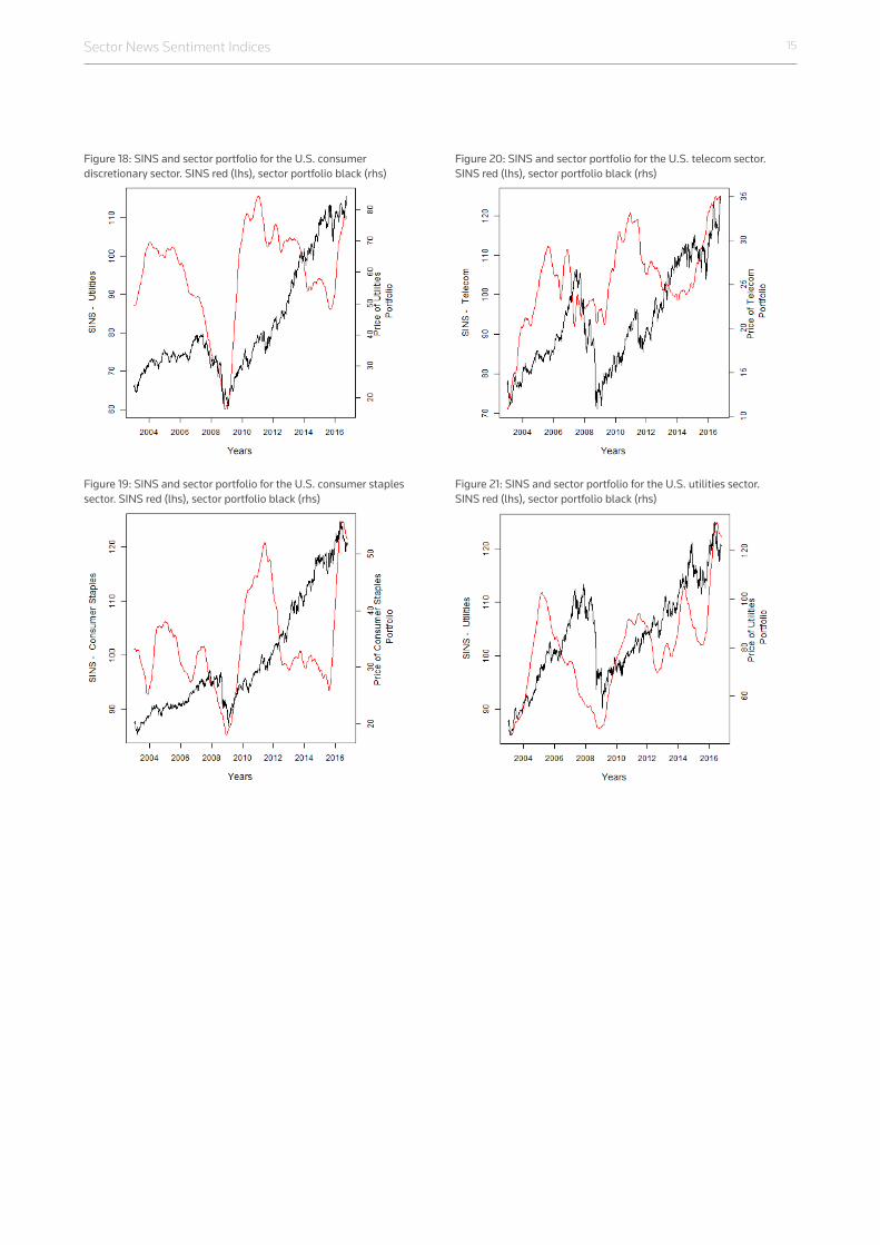
Figure 18: SINS and sector portfolio for the U.S. consumer discretionary sector. SINS red (lhs), sector portfolio black (rhs)

Figure 19: SINS and sector portfolio for the U.S. consumer staples sector. SINS red (lhs), sector portfolio black (rhs)

Figure 20: SINS and sector portfolio for the U.S. telecom sector. SINS red (lhs), sector portfolio black (rhs)

Figure 21: SINS and sector portfolio for the U.S. utilities sector. SINS red (lhs), sector portfolio black (rhs)


Figure 22: Plots of coefficients from quantile regression for energy sector; red solid line indicates OLS estimate

Figure 23: Plots of coefficients from quantile regression for health care sector; red solid line indicates OLS estimate

Figure 24: Plots of coefficients from quantile regression for industrial sector; red solid line indicates OLS estimate

Figure 25: Plots of coefficients from quantile regression for materials sector; red solid line indicates OLS estimate

Figure 26: Plots of coefficients from quantile regression for real estate sector; red solid line indicates OLS estimate

Figure 27: Plots of coefficients from quantile regression for consumer staples sector; red solid line indicates OLS estimate

Figure 28: Plots of coefficients from quantile regression for telecom sector; red solid line indicates OLS estimate

Figure 29: Plots of coefficients from quantile regression for utilities sector; red solid line indicates OLS estimate

Visit financial.tr.com

S055198/1-18

sector news sentiment indices - …€¦ · the gics classification covers 11 sectors, 24 industry...

Documents