sector based linear regression, a new robust method for

Acta Cybernetica 23 (2018) 1017–1038.

Sector Based Linear Regression, a New Robust

Method for the Multiple Linear Regression

Gabor Nagya

Abstract

This paper describes a new robust multiple linear regression method,which based on the segmentation of the N dimensional space to N+1 sec-tor. An N dimensional regression plane is located so that the half (or other)part of the points are under this plane in each sector. This article also presentsa simple algorithm to calculate the parameters of this regression plane. Thisalgorithm is scalable well by the dimension and the count of the points, andcapable to calculation with other (not 0.5) quantiles. This paper also con-tains some studies about the described method, which analyze the result withdifferent datasets and compares to the linear least squares regression.

Sector Based Linear Regression (SBLR) is the multidimensional general-ization of the mathematical background of a point cloud processing algorithmcalled Fitting Disc method, which has been already used in practice to pro-cess LiDAR data. A robust regression method can be used also in many otherfields.

Keywords: linear regression, robust regression, quantile regression

1 Introduction

The linear regression is an important component in a lot of calculation in the scienceand the engineering practice. This tool makes a relationship between one or moreindependent and one dependent variables by a linear function according to a givendataset.

The most popular method of the linear regression uses the least squares ap-proach for fitting a line (or a plane in higher dimensions) to the given dataset.The outlier points makes remarkable impact in the result of the least squares basedregression method.

There are some robust method of the linear regression [18, 21, 17, 22], forexample, the Random Sample Consensus (RANSAC) method [6, 4, 7] and theTheil-Sen estimator [19, 23].The complexity of the RANSAC method is increased

aObuda University, Alba Regia Technical Faculty, Institute of Geoinformatics, E-mail:[email protected]

DOI: 10.14232/actacyb.23.4.2018.3

1018 Gabor Nagy

Figure 1: The sectors in case of N = 1. (The N = 1 is the number of theindependent values, the total dimension of the space is N + 1 = 2, because thedependent value increases the dimension.) The area is divided to two parts (by thedashed line). The centres of this sectors are displayed by dotted lines.

highly with the dimension in the multiple linear regression, because(NM

)different

planes can be fitted to M given points in an N dimensional space. Both of thesemethods are not suitable for using with different quantiles.

This article describes the Sector Based Linear Regression (SBLR), a new robustmethod for the multiple linear regression. The SBLR method runs O

(MN3

)time,

where M the number of the points of the dataset, and N is the number of theindependent variables. The dimension of the space will be N + 1 with the onedependent variable. The SBLR can be used with different quantiles, for examplea regression line over the 10 percent (q = 0.1) of the points, as other quantileregression methods [12, 23, 1].

2 Principles of the method

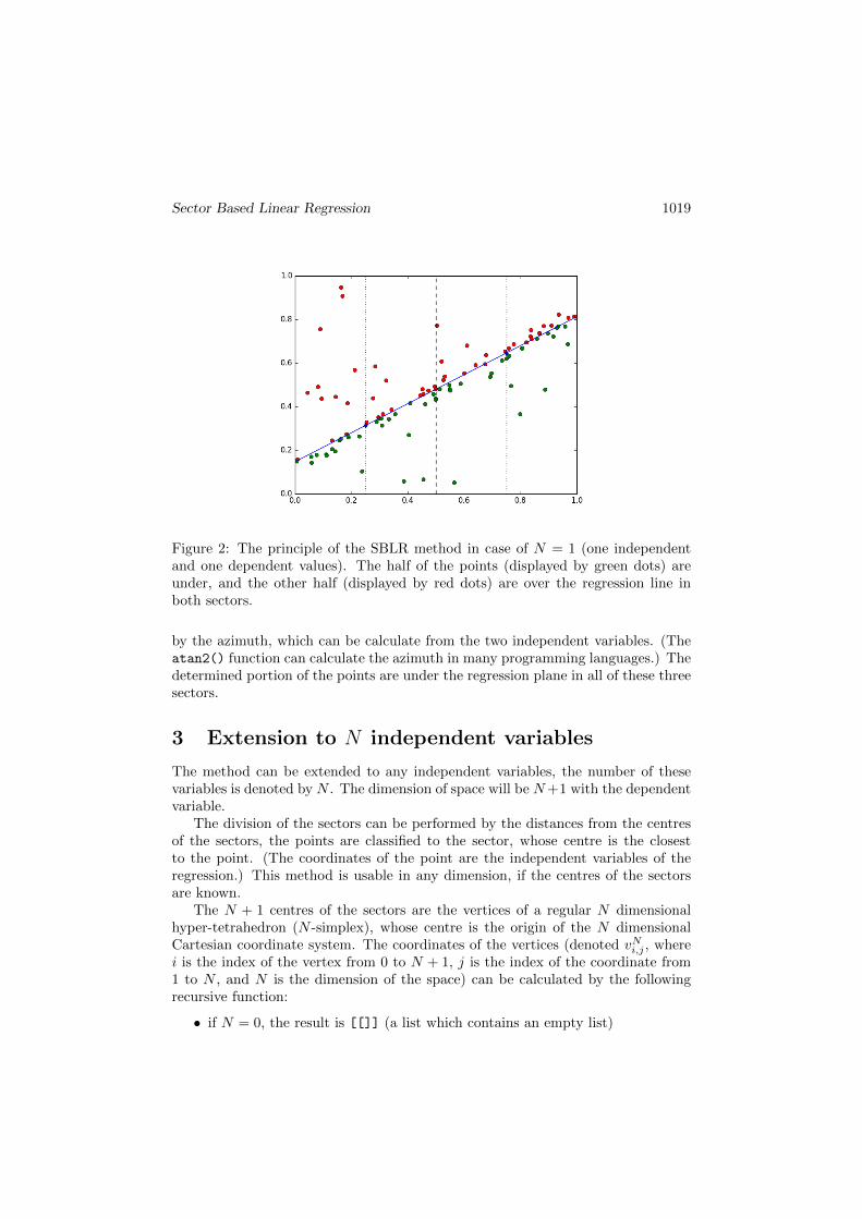
In the simple linear regression (one independent variable and one dependent vari-able, N = 1), the regression line has two parameters, for example the a and the b inthe y = ax+ b equation. The plane can be divided into two parts (in the following:sectors) by a line parallel to the y axis (Figure 1.). A regression line are searchedwhere the half (q = 0.5) or the other portion of the points are under the line inboth sectors (Figure 2.).

In case of the regression planes (two independent variables and one dependentvariable, N = 2), the plane of the two independent variable can be divided tothree 120 degrees angles as sectors (see Figure 3.). The division can be performed

Sector Based Linear Regression 1019

Figure 2: The principle of the SBLR method in case of N = 1 (one independentand one dependent values). The half of the points (displayed by green dots) areunder, and the other half (displayed by red dots) are over the regression line inboth sectors.

by the azimuth, which can be calculate from the two independent variables. (Theatan2() function can calculate the azimuth in many programming languages.) Thedetermined portion of the points are under the regression plane in all of these threesectors.

3 Extension to N independent variables

The method can be extended to any independent variables, the number of thesevariables is denoted by N . The dimension of space will be N+1 with the dependentvariable.

The division of the sectors can be performed by the distances from the centresof the sectors, the points are classified to the sector, whose centre is the closestto the point. (The coordinates of the point are the independent variables of theregression.) This method is usable in any dimension, if the centres of the sectorsare known.

The N + 1 centres of the sectors are the vertices of a regular N dimensionalhyper-tetrahedron (N -simplex), whose centre is the origin of the N dimensionalCartesian coordinate system. The coordinates of the vertices (denoted vNi,j , wherei is the index of the vertex from 0 to N + 1, j is the index of the coordinate from1 to N , and N is the dimension of the space) can be calculated by the followingrecursive function:

• if N = 0, the result is [[]] (a list which contains an empty list)

1020 Gabor Nagy

Figure 3: The sectors in case of N = 2. This figure represents the plane of the twoindependent variables, the coordinate of the dependent variable is perpendiculat tothis plane. The half (or other quantile) of the points are under the regression planein all sectors. (The points of the different sectors are displayed by different colors)This case is used in the LiDAR data processing where the points are the points ofthe LiDAR point cloud, the independent values are the horizontal coordinates ofthe points and the dependent coordinate is the vertical coordinate.


Figure 4: Calculate the coordinates of the vertices of an N -dimensional hyper-tetrahedron. (where 1 ≤ N ≤ 3)

• if N > 0, the coordinates of the vertices are calculated by this expression:

vNi,j =

vN−1i,j

√1− 1

N if i < N + 1 and j < N

− 1N if i < N + 1 and j = N

0 if i = N + 1 and j < N

1 if i = N + 1 and j = N

(1)

If N = 1 then v11,1 = −1 and v12,1 = 1. If N = 2 then v21,1 = −√22 , v21,2 = − 1

2 ,

v21,1 =√22 , v21,2 = − 1

2 , v21,1 = 0 and v21,2 = 1. (Figure 4.)

These vertices are at 1 unit distance from the origin of the coordinate system.The sectors centres are N

N+1 units from the origin, because this point is the nearestto the centres of the sector. The sectors are indexed from 0 to N . The coordinatesof the sector centres are:

sNi,j =N

N + 1vNi+1,j (2)

The N + 1 dimensional regression hyperplane can be specified by N + 1 valuein two ways. One of them is a linear expression:

h = l0 + l1x1 + l2x2 + · · ·+ ljxj + · · ·+ lNxN (3)

1022 Gabor Nagy

where xj is the coordinates of the position (the independent values, j indexedfrom 1 to N), and lj is the N + 1 coefficients of the N dimensional hyperplane (jindexed from 0 to N) in a N + 1 dimensional space.

The other way to define the independent values (the elevations of the plane) inthe N + 1 centres of the sectors (the vertices of the N dimensional regular hyper-tetrahedron), which are denoted ci, where i is the index of the vertex from 0 to N .The vector of ci values (denoted c) can be calculated simply from the vector of ljvalues (denoted l):

c = Q · l (4)

And the l can be calculated from the c, if both sides of (4) are multipled left-hand side by Q−1:

l = Q−1 · c (5)

The 4 and the 5 link between heights of sector’s centres and coefficients of thelinear equation of the hyperplane.

The Q is an N + 1×N + 1 size matrix:

Q =

1 sN0,1 · · · sN0,j · · · sN0,N−1 sN0,N1 sN1,1 · · · sN1,j · · · sN1,N−1 sN1,N...

.... . .

.... . .

......

1 sNi,1 · · · sNi,j · · · sNi,N−1 sNi,N...

.... . .

.... . .

......

1 sNN−1,1 · · · sNN−1,j · · · sNN−1,N−1 sNN−1,N1 sNN,1 · · · sNN,j · · · sNN,N−1 sNN,N

The Q−1 is the inverse of Q, and can be calculated in O

(N3)

time. Because the

Q contains only constant values (the coordinates of the sector centres, and 1 values),

the program has to calculate the matrix inversion only once. The multiplications(in (4) and (5)) need O

(N2)

time.

4 The calculation method

There is a given dataset, which contains M points. Each point contains N inde-pendent values (the coordinates in an N dimensional space) and one dependentvalue (which is an extra dimension). In the following, pk,j notation is used for theindependent variables of the points, where k is the index of the point from 0 toM − 1, and the j is the index of the coordinates from 1 to N . The pk,0 values arethe dependent variables.


4.1 Normalization

The first step is the normalization of the coordinates to the [−1,+1] interval by thexj = ajX+bj expression. If one regression will be calculated for all points, calculatethe normalized coordinates with aj = 2

max(xj)−min(xj)and bj = −1−min (xj) aj .

In another case, the regression will be calculated a selected part of the dataset.The points, which are nearest to a specified position (specified an r vector, whose

elements are rj) than a defined R radius (R2 ≤∑Nj=1 (xj − rj)

2). In this case, the

aj = 1R and the bj = −rj .

In the following steps, the program uses these normalized coordinates.

4.2 Separating into sectors

In the next step, the points will be separated into the sectors, and calculate theinitial value of the sector centres (ci). Each points put the sector whose centre isthe closest to the point. I use pi,k,j notation in the separated dataset, where i isthe index of the sector (from 0 to N) and k is the number of the point in the sectorfrom 1 to mi.

All of the sectors have to contain at least one point (∀ i mi > 0). If any sectordoes not contain any point (∃ i mi = 0), the method can not work. This can happen,when the number or the dispersion of the points is not suitable. The probability ofthe any empty sector, when the dispersion is random (the P (point in the sector) =

1N+1 in all of the sectors) is P (any empty sector) = 1−

(1−

(NN+1

)M)N+1

.

The initial values of the sector’s centres (ci) are the defined quantile (q) of thedependent variables of the sector’s points:

ci = quantile ([pi,1,0, pi,2,0, . . . , pi,mi,0] , q) (6)

These values determines the initial regression plane. (See the Figure 5. in caseof N = 1.)

4.3 The iteration steps

The key element of the method is an iteration step. The program goes from sectorto sector and calculates the new values of the sector’s centre.

Many N + 1 dimensional hyperplanes can be calculated, which are fitted tothe centres of the other sectors and each points of the sector. The row of thesector’s centre in the Q matrix has to be changed to the coordinates of the point

([pi,k,1, pi,k,2, . . . , pi,k,N ]), and the ci value has to be changed to the pi,k,0 (k isthe index of the point in the sector) in the c vector, and use this modified (5) tocalculate the parameters of the hyperplane. After calculating of the hyperplaneparameters (lj), calculate and store the the elevation of this plane in the sectorcentre by the (3):

1024 Gabor Nagy

Figure 5: The initial step in case of N = 1. The median values are calculatedfor both sectors. (upper figure) These values (displayed by diamonds) will be theheight of the initial regression line in the center of the sectors (dotted line). Thepoints are displayed by red dots over and green dots under the lines (the height ofthe median, and the initial regression line). The initial regression line is fitted tothe centre points. (lower figure)


hk = l0 + l1pi,k,1 + l2pi,k,2 + · · ·+ ljpi,k,j + · · ·+ lNpi,k,N (7)

The new value of the sector’s centre is the defined quantile (q) of these values:

cnewi = quantile ([h1, h2, . . . , hmi ] , q)

The program continues this process in the sector number (i + 1) mod N + 1, and check the difference between the new and the old ci values. If the differenceless than a specified value (

∣∣coldi − cnewi

∣∣ < ε), a counter is increased one, otherwisethe counter set to zero. The iteration loop is repeated while this counter is lessthan N + 1. (The first two step in case of N = 1 is presented in Figure 6.)

The changes of the heights of the sector’s centres typically will be less in theiterations. This ensures convergence.

4.4 Completion

Finally, the parameters of the regression plane are calculated by the (5) from thecentres of the sectors. The received parameters are in a normalized coordinatesystem. (See 4.1)

If only the elevation of the plane is needed in the origin of the normalizedcoordinate system, the l0 is this. If the plane equation is needed in the originalcoordinate system, the liai expression can be used.

5 Studying the SBLR algorithm

Some simple Python [20, 16, 14] programs were made to test the SBLR algorithm.The sblr.py module is a simple implementation of the SBLR method. The testprograms use this module.

The test programs use random datasets, which are created by the random

Python module. This module can generate random numbers with several distri-bution. In the following studies the test programs use the y = 3x − 5 linear basefunction. The independent values (x) are generated by a uniform random valuebetween 0 and 10 (random.uniform(0,10)). The dependent values are calculatedby the y = 3x − 5 + error equation. The error is various random number with1 standard deviation and 0 median. A specific part of the points are outlier; thedependent variable of this points is a uniform random value between −7 and 27.

The test programs use different random numbers for the error value based onthe random Python module. The uniform distribution error is a random number be-tween −

√3 and

√3 by the random.uniform(-1,1)*1.7320508075688772 expres-

sion. The normal distribution uses random.normalvariate(1,0), the lognormaldistribution uses random.lognormalvariate(1,0)-1 and the exponential distribu-tion uses random.expovariate(1)-0.6931471805599453. The minus 1 and minus0.6931471805599453 ' ln (2) need for the 0 median.

1026 Gabor Nagy

Figure 6: The iteration steps in case of N = 1. The new values of the sector’scentres are determined so that the half (or other quantile) of the sector’s pointswill be under the line, which is fitted the new centre of this sector and the othersector’s centre. The new line is continuous, the line of the last iteration is dotted.The iteration is repeated until the change of the values are less than a limit (denotedε) in both sectors.


Figure 7: The result of the SBLR method (dashed line) and the least squares linearregression (dotted line) in a dataset with many outlier points.

5.1 Comparsion to the least squares linear regression

The least squares method is the most common regression tool, but the any outliermeasurements can indicate significant difference in the result. (Figure 7.) A re-gression line can be calculated by the least squares method, the sum of squares ofthe differences between the points and the regression line will be the smallest withthis regression line.

A test program generated random datasets with different portion of outlierpoints (from 0 to 75 percent). The test program generated 5000 datasets in all out-lier portion (0%, 1%, 2%, ... 75%) and calculated regression lines in each dataset bythe SBLR and the least squares methods. The two regression lines were comparedto the original line, and calculate the averages of the distance from this line in the[0, 10] interval. This number was the metrics of the fitting in these studies.

In each outlier portion, the test program stored 5000 fitting value; and anotherprogram calculated the averages of these values in both methods in each outlierportion. The Figure 8. shows the result of these studies with different number ofpoints.

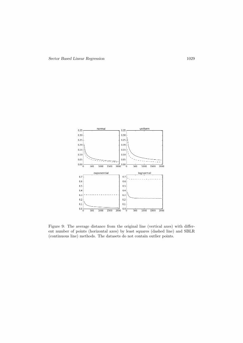
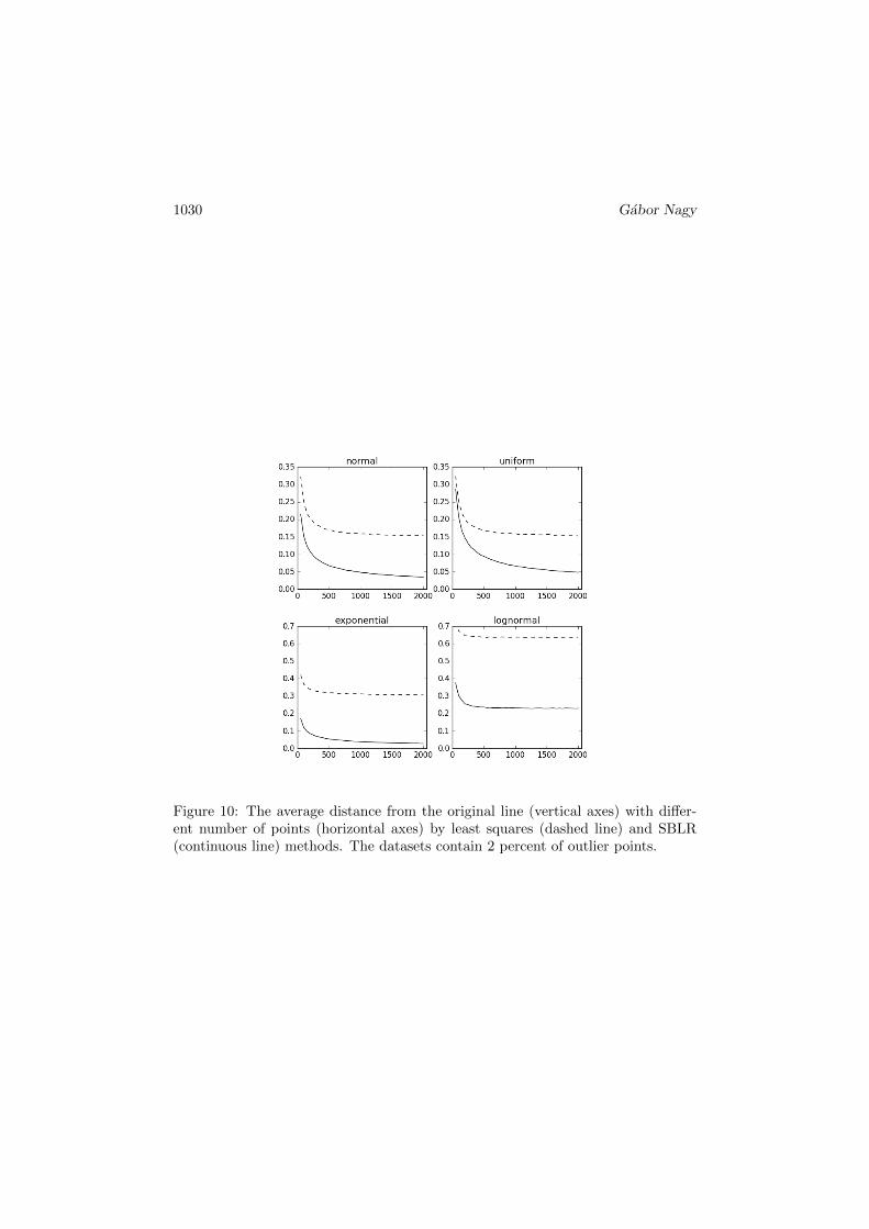
Another studies compare the average distance with different count of the pointsand different distribution of errors. The point numbers were the elements from anarithmetic sequence from 50 to 2000 with step of 50. The studies made with differ-ent errors (normal, uniform, lognormal and exponential) and different percentageof outliers (0 and 2). The program generates 5000 random datasets in each case.The result of these studies are seen in the Figure 9. and Figure 10.

1028 Gabor Nagy

Figure 8: The average distance from the original line and the percentage of outlierswith different number of points (100, 200 and 500) by least squares (dashed line)and SBLR method (dotted line). The range between 0 and 10 percent is zoom inon the lower figure.


Figure 9: The average distance from the original line (vertical axes) with differ-ent number of points (horizontal axes) by least squares (dashed line) and SBLR(continuous line) methods. The datasets do not contain outlier points.

1030 Gabor Nagy

Figure 10: The average distance from the original line (vertical axes) with differ-ent number of points (horizontal axes) by least squares (dashed line) and SBLR(continuous line) methods. The datasets contain 2 percent of outlier points.


In the asymmetric error distributions (exponential and lognormal), the SBLRcreated better result than the least squares method without outlier points. If thedataset has 2 percent of outlier points, the SBLR made better result in all of theexamined error distributions.

5.2 Examining the iteration steps

The computation time of the SBLR method grows linearly with the count of thepoints (denoted M in this article). This computation time may be increased if theiteration steps of the method grows with M .

Some test programs were created to study the correlation between the numberof the points and the iteration steps. The M was different values according to ageometric sequence. The initial value of this sequence is 100 and the common ratiois 4√

2 ' 1.1892 (the result was rounded). The largest datasets had 102400 points.

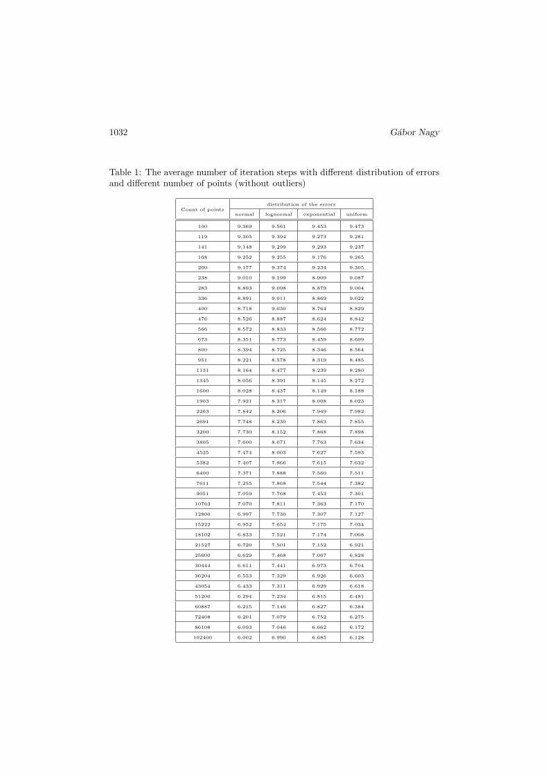
The test programs created 1000 different random datasets with each M and eachdistributions, calculated the regression lines and store the number of the iterationsteps with ε = 10−5. Another program analyzed the stored data and calculate themeans of the iteration steps. (Table 1.)

The number of the iteration step does not grow, moreover a little decrease,when the M increased. The computation time of the SBLR method is O

(MN3

).

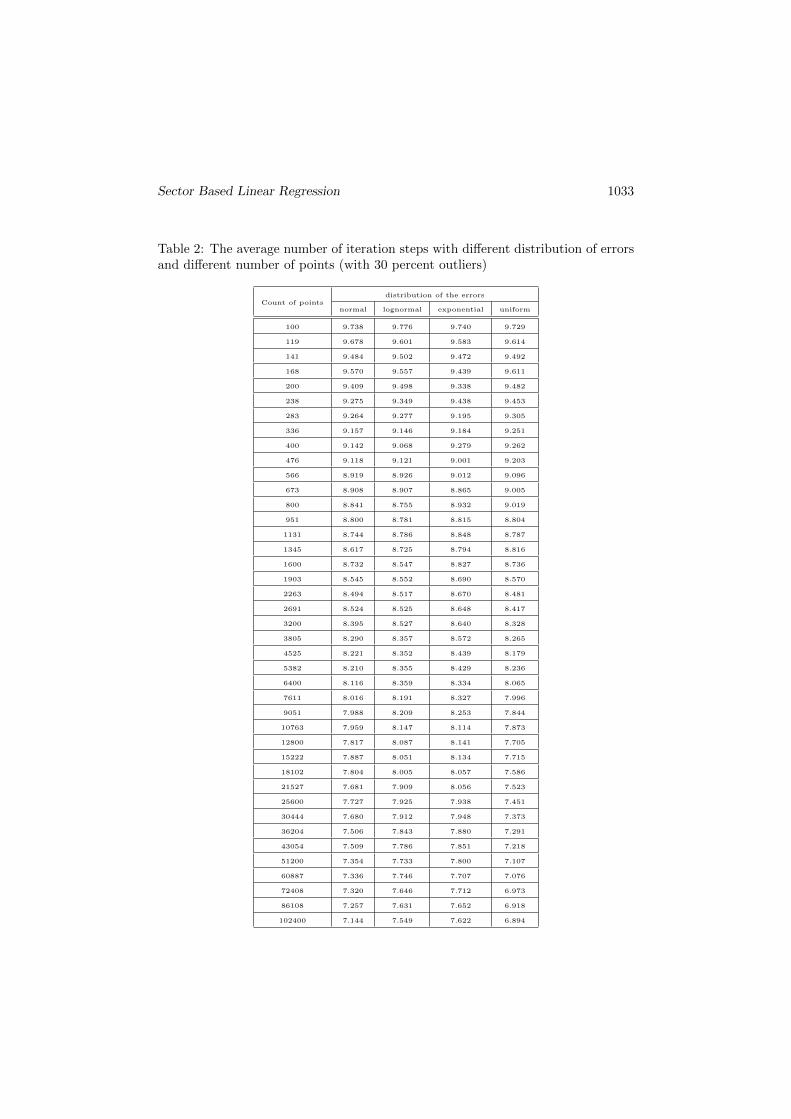
The result is same when the 30 percent of the points are outlier. Other parameterswere not changed. (Table 2.)

5.3 The limits and possible errors of the SBLR method

The SBLR method can calculate only linear regression, and only one regressionin a dataset. The Ref. [10] presents a method, which can be found more linearregression from one dataset.

The method can work if all sectors have at least one point. The good resultneeds more points in all sectors to eliminate the impact of the outliers.

An outlier point may result wrong sector layout. The normalization step (see in4.1) create a wrong result, where the outlier point is in a sector, and all the rest inthe other sector. This problem can be avoided, if the sector centre is determined asthe median of the values. In the practical applications (in the author’s practice),this mistake has not occurred, because the points are selected from a bigger dataset(see in 6.1), therefore it did not have far points in the independent coordinates.

6 Application possibilities

The SBLR has a lot of application possibilities. This method may be used inprojects, where need a robust linear regression. The SBLR may be useful, whenquantile regression are needed in any dimension spaces.

1032 Gabor Nagy

Table 1: The average number of iteration steps with different distribution of errorsand different number of points (without outliers)

Count of pointsdistribution of the errors

normal lognormal exponential uniform

100 9.369 9.561 9.453 9.473

119 9.305 9.394 9.273 9.281

141 9.148 9.299 9.293 9.237

168 9.252 9.255 9.176 9.265

200 9.177 9.374 9.234 9.305

238 9.010 9.199 8.909 9.087

283 8.893 9.098 8.879 9.004

336 8.891 9.011 8.869 9.022

400 8.718 9.030 8.764 8.829

476 8.526 8.887 8.624 8.842

566 8.572 8.833 8.566 8.772

673 8.351 8.773 8.459 8.609

800 8.394 8.725 8.346 8.564

951 8.221 8.578 8.319 8.485

1131 8.164 8.477 8.239 8.280

1345 8.056 8.391 8.145 8.272

1600 8.028 8.437 8.149 8.188

1903 7.921 8.317 8.008 8.023

2263 7.842 8.206 7.949 7.982

2691 7.748 8.230 7.863 7.855

3200 7.730 8.152 7.868 7.898

3805 7.600 8.071 7.763 7.634

4525 7.474 8.003 7.627 7.593

5382 7.407 7.966 7.615 7.632

6400 7.371 7.888 7.560 7.511

7611 7.255 7.868 7.544 7.382

9051 7.059 7.768 7.453 7.301

10763 7.070 7.811 7.363 7.170

12800 6.997 7.730 7.307 7.127

15222 6.952 7.654 7.175 7.034

18102 6.833 7.521 7.174 7.008

21527 6.720 7.501 7.152 6.921

25600 6.629 7.468 7.067 6.828

30444 6.611 7.441 6.973 6.704

36204 6.553 7.329 6.926 6.603

43054 6.433 7.311 6.929 6.618

51200 6.294 7.234 6.815 6.481

60887 6.215 7.146 6.827 6.384

72408 6.201 7.079 6.752 6.275

86108 6.093 7.046 6.662 6.172

102400 6.002 6.990 6.685 6.128


Table 2: The average number of iteration steps with different distribution of errorsand different number of points (with 30 percent outliers)

Count of pointsdistribution of the errors

normal lognormal exponential uniform

100 9.738 9.776 9.740 9.729

119 9.678 9.601 9.583 9.614

141 9.484 9.502 9.472 9.492

168 9.570 9.557 9.439 9.611

200 9.409 9.498 9.338 9.482

238 9.275 9.349 9.438 9.453

283 9.264 9.277 9.195 9.305

336 9.157 9.146 9.184 9.251

400 9.142 9.068 9.279 9.262

476 9.118 9.121 9.001 9.203

566 8.919 8.926 9.012 9.096

673 8.908 8.907 8.865 9.005

800 8.841 8.755 8.932 9.019

951 8.800 8.781 8.815 8.804

1131 8.744 8.786 8.848 8.787

1345 8.617 8.725 8.794 8.816

1600 8.732 8.547 8.827 8.736

1903 8.545 8.552 8.690 8.570

2263 8.494 8.517 8.670 8.481

2691 8.524 8.525 8.648 8.417

3200 8.395 8.527 8.640 8.328

3805 8.290 8.357 8.572 8.265

4525 8.221 8.352 8.439 8.179

5382 8.210 8.355 8.429 8.236

6400 8.116 8.359 8.334 8.065

7611 8.016 8.191 8.327 7.996

9051 7.988 8.209 8.253 7.844

10763 7.959 8.147 8.114 7.873

12800 7.817 8.087 8.141 7.705

15222 7.887 8.051 8.134 7.715

18102 7.804 8.005 8.057 7.586

21527 7.681 7.909 8.056 7.523

25600 7.727 7.925 7.938 7.451

30444 7.680 7.912 7.948 7.373

36204 7.506 7.843 7.880 7.291

43054 7.509 7.786 7.851 7.218

51200 7.354 7.733 7.800 7.107

60887 7.336 7.746 7.707 7.076

72408 7.320 7.646 7.712 6.973

86108 7.257 7.631 7.652 6.918

102400 7.144 7.549 7.622 6.894

1034 Gabor Nagy

Figure 11: The application of the SBLR method in LiDAR data processing withdifferent R and q values.

6.1 LiDAR data processing

SBLR can be used in any application, where a robust linear regression method isrequired. If the distribution of the measurement error is skewed, the method canuse a different q value than 0.5.

This method has been used for processing the LiDAR point clouds. In this case(N = 2), the two independent value are the horizontal coordinates, the dependentvariable is the elevation, and the measurements are the points of the LiDAR pointcloud. (See the Figure 3.) The classical X, Y , and Z coordinates of the points aredenoted x1, x2 and h in this case in the equation of a fitting plane, and pk,1, pk,2and pk,0 in the point of the cloud.

The regression plane is fitted to a part of the total LiDAR cloud, which is cutby a circle shape with R radius. The regression plane fits to this part of the cloud,because this method is called “Fitting Disc” method. [15] This principle may beused in other cases, where the connection is not linear between the independent andthe dependent values: select the points, which are nearest than a radius (R) froman examined position, and fit a linear, N dimensional plane to this part, which isapproximately linear. (See in the Figure 12., in a two-dimensional illustration.) TheFitting Disc method is a local application of the Sector Based Linear Regression.

Digital Elevation Models can be created, if the SBLR based Fitting Disc methodis applied in each point of the DEM grid. The result depends from R and q values,for example the Figure 11. In the forest areas the appropriate result needs very low


Figure 12: The LiDAR data processing with SBLR in a two-dimensional illustra-tion. The ground surface is evaluated by q = 0.1 parameter, because the majorityof the points are in the trees and bushes, over the ground surface.

q values; and the very low q values need long R radius, because some points mustbe under the plane. If the intention is at least on average n points under the plane

in each sectors, the radius is R =√

3nqdπ , where d is the density of the LiDAR point

cloud in points/m2.The SBLR based Fitting Disc method can be applied to recognize planes in a

point cloud, for example the roofs of the buildings. In these cases the plane of thedetected object (for example a roof) can be calculated by SBLR from a segment ofthe point cloud.

6.2 Other possibilities

A linear regression plane can be fitted to the data of the pixels of a picture neara position (like the LiDAR data processing) and calculated a filtered color by thisregression plane. This filtering method is same as the Two-Dimensional MedianFiltering Algorithm [8].

The SBLR can be used for any data processing task, where a linear regressionis needed in an N -dimensional space. This method can be used well with a lot ofoutlier data or a random error with asymmetric distribution.

The SBLR is a linear case of the quantile regression [13, 12, 11]. The quantileregression is used in different disciplines, for example ecology [3] or economy [2, 5].

A robust linear regression method can provide a robust method to determine theparameters an affine transformation by control points. This calculation needs twoindependent linear regression for the two coordinates (in case of the two-dimensionalaffine transformation), because each equations of the affine transformation are a lin-

1036 Gabor Nagy

ear regression, where the independent variables are the coordinates of the referencesystem one, and the dependent variable is a coordinate of the reference system two.

7 Conclusions and future work

The Sector Based Linear Regression is a robust method for fitting an N dimensionalhyperplane to a dataset which has N independent and 1 dependent variables. Thestudies of this article focused to the simple N = 1 case, and the practical application(LiDAR data processing) uses the N = 2 case, but the method can be applied inany dimension. This method provides quantile regression, it is useful in some cases(for example the LiDAR data processing, when the majority of the points are overthe ground surface).

The processing time of the SBLR method is increased only linear with the sizeof the input data (the number of the points, denoted by M in this article). Thisadvantage makes it ideal for big data processing applications.

This article presents the principle of the method, an algorithm for the SBLR,and some studies and application possibilities of the method. A simple implementa-tion of the SBLR method has been made. The source code of this Python 3 moduleis attached to this article. In the future, i would like to implement the method inother programming languages, and improve the efficiency of the program.

The principle of the Sector Based Linear Regression can be adapted to non-linear regressions. The area must be divided more sectors in these cases, becausethe non-linear curves need more parameters.

8 Acknowledgement

This research was supported by the project number TAMOP-4.2.2.B-15/1/KONV-2015-0010, titled “Tudomanyos kepzes muhelyeinek fejlesztese az Alba Regia Mu-szaki Karon” (in English: Developing workshops of the scientific education in theAlba Regia Technical Faculty).

The Figure 1., Figure 2., Figure 5., Figure 6, Figure 7., Figure 8., Figure 9.,Figure 10. and Figure 11. were created by Matplotlib [9].

9 Additional files

This article contains two animated GIF files. The sblr.gif shows the SBLRmethod during operation in case of N = 1. The fitdisc.gif presents the testarea of the Figure 11. in many other cases of R and q parameters of the FittingDisc method.

The implemented SBLR algorithm is already attached sblr.py Python 3 mod-ule. This module provides the SBLR calculations in any Python 3 program.


References

[1] Bertsimas, Dimitris and Mazumder, Rahul. Least quantile regression via mod-ern optimization. The Annals of Statistics, pages 2494–2525, 2014.

[2] Buchinsky, Moshe. Changes in the us wage structure 1963-1987: Application ofquantile regression. Econometrica: Journal of the Econometric Society, pages405–458, 1994.

[3] Cade, Brian S and Noon, Barry R. A gentle introduction to quantile regressionfor ecologists. Frontiers in Ecology and the Environment, 1(8):412–420, 2003.

[4] Choi, Sunglok, Kim, Taemin, and Yu, Wonpil. Performance evaluation ofransac family. Journal of Computer Vision, 24(3):271–300, 1997.

[5] Coad, Alex and Rao, Rekha. Innovation and firm growth in high-tech sectors:A quantile regression approach. Research policy, 37(4):633–648, 2008.

[6] Fischler, Martin A and Bolles, Robert C. Random sample consensus: aparadigm for model fitting with applications to image analysis and automatedcartography. Communications of the ACM, 24(6):381–395, 1981.

[7] Hast, Anders, Nysjo, Johan, and Marchetti, Andrea. Optimal ransac-towardsa repeatable algorithm for finding the optimal set. 2013.

[8] Huang, T, Yang, G, and Tang, G. A fast two-dimensional median filteringalgorithm. IEEE Transactions on Acoustics, Speech, and Signal Processing,27(1):13–18, 1979.

[9] Hunter, J. D. Matplotlib: A 2d graphics environment. Computing In Science& Engineering, 9(3):90–95, 2007.

[10] Isack, Hossam and Boykov, Yuri. Energy-based geometric multi-model fitting.International journal of computer vision, 97(2):123–147, 2012.

[11] Jureckova, Jana. Robust quantile regression. Encyclopedia of Environmetrics,2006.

[12] Koenker, Roger. Quantile regression. Number 38. Cambridge university press,2005.

[13] Koenker, Roger and Bassett Jr, Gilbert. Regression quantiles. Econometrica:journal of the Econometric Society, pages 33–50, 1978.

[14] Millman, K Jarrod and Aivazis, Michael. Python for scientists and engineers.Computing in Science & Engineering, 13(2):9–12, 2011.

[15] Nagy, Gabor, Tamas, Jancso, and Chen, Chongcheng. The fitting disc method,a new robust algorithm of the point cloud processing. ACTA POLYTECH-NICA HUNGARICA, 14(6):59–73, 2017.

1038 Gabor Nagy

[16] Oliphant, Travis E. Python for scientific computing. Computing in Science &Engineering, 9(3), 2007.

[17] Rousseeuw, Peter J and Hubert, Mia. Regression depth. Journal of the Amer-ican Statistical Association, 94(446):388–402, 1999.

[18] Rousseeuw, Peter J and Leroy, Annick M. Robust regression and outlier de-tection, volume 589. John Wiley & Sons, 2005.

[19] Theil, Henri. A rank-invariant method of linear and polynomial regressionanalysis. In Henri Theils Contributions to Economics and Econometrics, pages345–381. Springer, 1992.

[20] Van Rossum, Guido et al. Python Programming Language. In USENIX AnnualTechnical Conference, volume 41, 2007.

[21] Wilcox, Rand R. Introduction to robust estimation and hypothesis testing.Academic press, 2011.

[22] Wilcox, Rand R and Keselman, HJ. Modern regression methods that cansubstantially increase power and provide a more accurate understanding ofassociations. European journal of personality, 26(3):165–174, 2012.

[23] Zhou, Weihua and Serfling, Robert. Multivariate spatial u-quantiles: Abahadur–kiefer representation, a theil–sen estimator for multiple regression,and a robust dispersion estimator. Journal of Statistical Planning and Infer-ence, 138(6):1660–1678, 2008.

Received 11th November 2017

sector based linear regression, a new robust method for

Documents