section i.2 lagrange’s equations - linearized eom’slagrange’s equations - linearized eom’s...

Chapter I: Linearized Lagrange’s Equations

I.2-1 ME 564 - Spring 20

Section I.2 Lagrange’s Equations - Linearized EOM’s

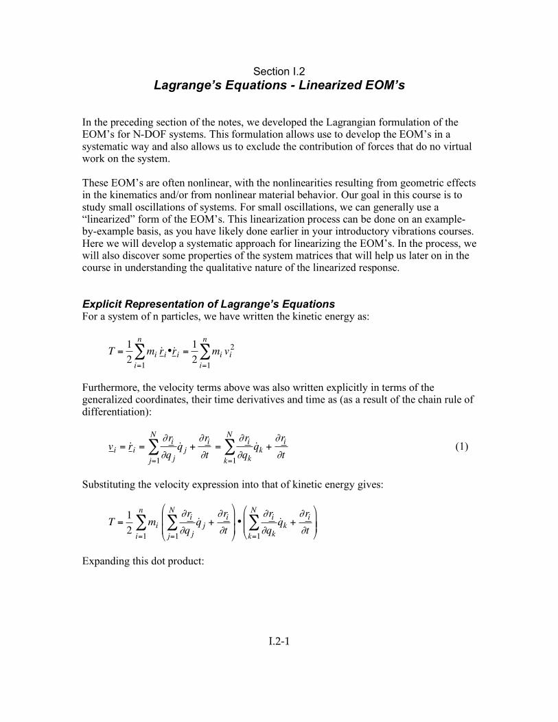
In the preceding section of the notes, we developed the Lagrangian formulation of the EOM’s for N-DOF systems. This formulation allows use to develop the EOM’s in a systematic way and also allows us to exclude the contribution of forces that do no virtual work on the system. These EOM’s are often nonlinear, with the nonlinearities resulting from geometric effects in the kinematics and/or from nonlinear material behavior. Our goal in this course is to study small oscillations of systems. For small oscillations, we can generally use a “linearized” form of the EOM’s. This linearization process can be done on an example-by-example basis, as you have likely done earlier in your introductory vibrations courses. Here we will develop a systematic approach for linearizing the EOM’s. In the process, we will also discover some properties of the system matrices that will help us later on in the course in understanding the qualitative nature of the linearized response. Explicit Representation of Lagrange’s Equations For a system of n particles, we have written the kinetic energy as:

!

T =1

2mi

˙ r i•˙ r i

i=1

n

" =1

2mi vi

2

i=1

n

"

Furthermore, the velocity terms above was also written explicitly in terms of the generalized coordinates, their time derivatives and time as (as a result of the chain rule of differentiation):

!

vi = ˙ r i ="ri

"q j

˙ q jj=1

N

# +"ri

"t=

"ri

"qk

˙ q kk=1

N

# +"ri

"t (1)

Substituting the velocity expression into that of kinetic energy gives:

!

T =1

2mi

"ri

"q j

˙ q jj=1

N

# +"ri

"t

$

%

& &

'

(

) )

•"ri

"qk

˙ q kk=1

N

# +"ri

"t

$

% & &

'

( ) )

i=1

n

#

Expanding this dot product:


I.2-2 ME 564 - Spring 20

!

T =1

2mi

"ri

"t•"ri

"t+"ri

"t•

"ri

"qk

˙ q kk=1

N

#$

% & &

'

( ) ) +

"ri

"q j

˙ q jj=1

N

#$

%

& &

'

(

) ) •"ri

"t+

"ri

"q j

˙ q jj=1

N

#$

%

& &

'

(

) ) •

"ri

"qk

˙ q kk=1

N

#$

% & &

'

( ) )

*

+ ,

- ,

.

/ ,

0 , i=1

n

#

=1

2mi

"ri

"t•"ri

"t+ 2

"ri

"t•

"ri

"qk

˙ q kk=1

N

#$

% & &

'

( ) ) +

"ri

"q j

˙ q jj=1

N

#$

%

& &

'

(

) ) •

"ri

"qk

˙ q kk=1

N

#$

% & &

'

( ) )

*

+ ,

- ,

.

/ ,

0 , i=1

n

#

=1

2mi

"ri

"t•"ri

"ti=1

n

# + mi

"ri

"t•

"ri

"qk

˙ q kk=1

N

#$

% & &

'

( ) )

i=1

n

# +1

2mi

"ri

"q j

˙ q jj=1

N

#$

%

& &

'

(

) ) •

"ri

"qk

˙ q kk=1

N

#$

% & &

'

( ) )

i=1

n

#

=1

2mi

"ri

"t•"ri

"ti=1

n

# + mi

"ri

"t•"ri

"qki=1

n

#$

% & &

'

( ) ) ˙ q k

k=1

N

# +1

2mi

"ri

"q j

•"ri

"qki=1

n

#$

% & &

'

( ) ) ˙ q j ˙ q k

k=1

N

#j=1

N

#

=1

2mi

"ri

"t•"ri

"ti=1

n

# + hk ˙ q kk=1

N

# +1

2m jk ˙ q j ˙ q k

k=1

N

#j=1

N

#

or

!

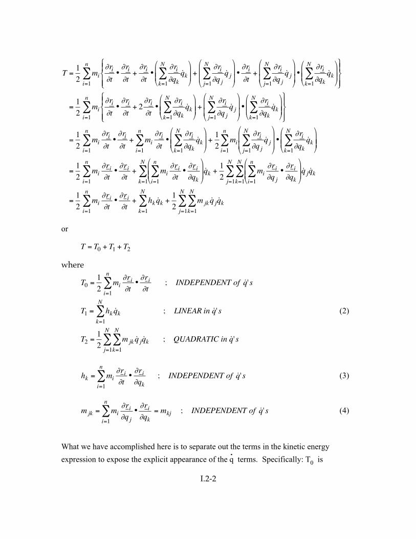
T = T0 + T1 + T2 where

!

T0 =1

2mi

"ri

"t•"ri

"ti=1

n

# ; INDEPENDENT of ˙ q 's

T1 = hk ˙ q kk=1

N

# ; LINEAR in ˙ q 's

T2 =1

2m jk ˙ q j ˙ q k

k=1

N

#j=1

N

# ; QUADRATIC in ˙ q 's

(2)

!

hk = mi

"ri

"t•"ri

"qki=1

n

# ; INDEPENDENT of ˙ q 's (3)

!

m jk = mi

"ri

"q j

•"ri

"qki=1

n

# = mkj ; INDEPENDENT of ˙ q 's (4)

What we have accomplished here is to separate out the terms in the kinetic energy expression to expose the explicit appearance of the q terms. Specifically: T0 is


I.2-3 ME 564 - Spring 20

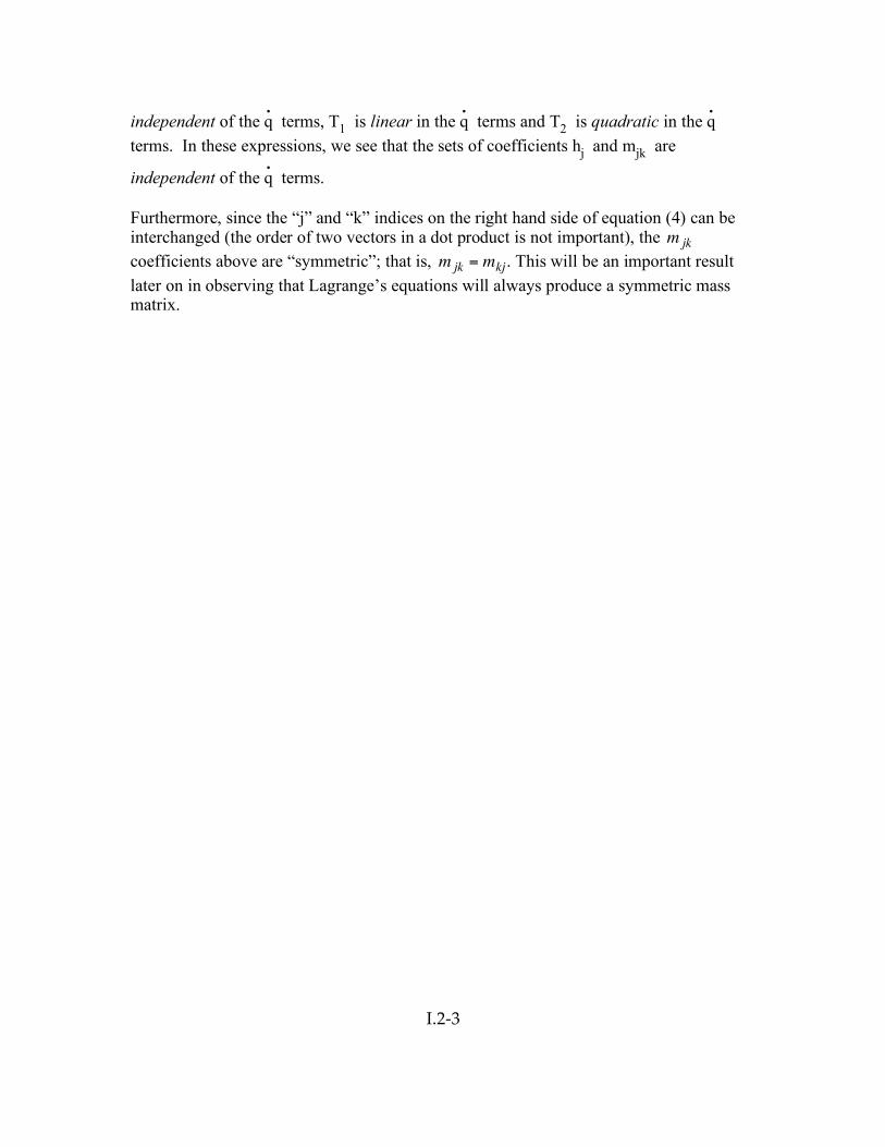
independent of the q terms, T1 is linear in the q terms and T2 is quadratic in the q terms. In these expressions, we see that the sets of coefficients hj and mjk are

independent of the q terms. Furthermore, since the “j” and “k” indices on the right hand side of equation (4) can be interchanged (the order of two vectors in a dot product is not important), the

!

m jk coefficients above are “symmetric”; that is,

!

m jk = mkj . This will be an important result later on in observing that Lagrange’s equations will always produce a symmetric mass matrix.


I.2-4 ME 564 - Spring 20

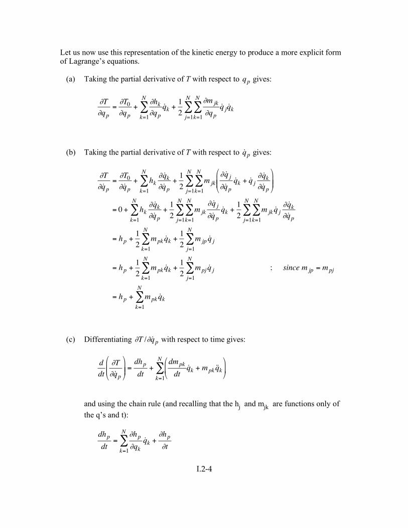
Let us now use this representation of the kinetic energy to produce a more explicit form of Lagrange’s equations.

(a) Taking the partial derivative of T with respect to

!

qp gives:

!

"T

"qp

="T0

"qp

+"hk

"qp

˙ q kk=1

N

# +1

2

"m jk

"qp

˙ q j ˙ q kk=1

N

#j=1

N

#

(b) Taking the partial derivative of T with respect to

!

˙ q p gives:

!

"T

" ˙ q p="T0

" ˙ q p+ hk

" ˙ q k

" ˙ q pk=1

N

# +1

2m jk

" ˙ q j

" ˙ q p˙ q k + ˙ q j

" ˙ q k

" ˙ q p

$

% & &

'

( ) )

k=1

N

#j=1

N

#

= 0 + hk

" ˙ q k

" ˙ q pk=1

N

# +1

2m jk

" ˙ q j

" ˙ q p˙ q k

k=1

N

#j=1

N

# +1

2m jk ˙ q j

" ˙ q k

" ˙ q pk=1

N

#j=1

N

#

= hp +1

2m pk ˙ q k

k=1

N

# +1

2m jp ˙ q j

j=1

N

#

= hp +1

2m pk ˙ q k

k=1

N

# +1

2m pj ˙ q j

j=1

N

# ; since m jp = m pj

= hp + m pk ˙ q kk=1

N

#

(c) Differentiating

!

"T /" ˙ q p with respect to time gives:

!

d

dt

"T

" ˙ q p

#

$ % %

&

' ( ( =

dhp

dt+

dm pk

dt˙ q k + m pk ˙ q k

#

$ %

&

' (

k=1

N

)

and using the chain rule (and recalling that the hj and mjk are functions only of

the q’s and t):

!

dhp

dt=

"hp

"qk

˙ q kk=1

N

# +"hp

"t


I.2-5 ME 564 - Spring 20

!

dm pk

dt=

"mpk

"q j

˙ q jj=1

N

# +"mpk

"t

gives:

!

d

dt

"T

" ˙ q p

#

$ % %

&

' ( ( =

"hp

"qk

˙ q kk=1

N

) +"hp

"t+

"mpk

"q j

˙ q jj=1

N

) +"mpk

"t

#

$

% %

&

'

( (

˙ q k + m pk ˙ q k

#

$

% %

&

'

( (

k=1

N

)

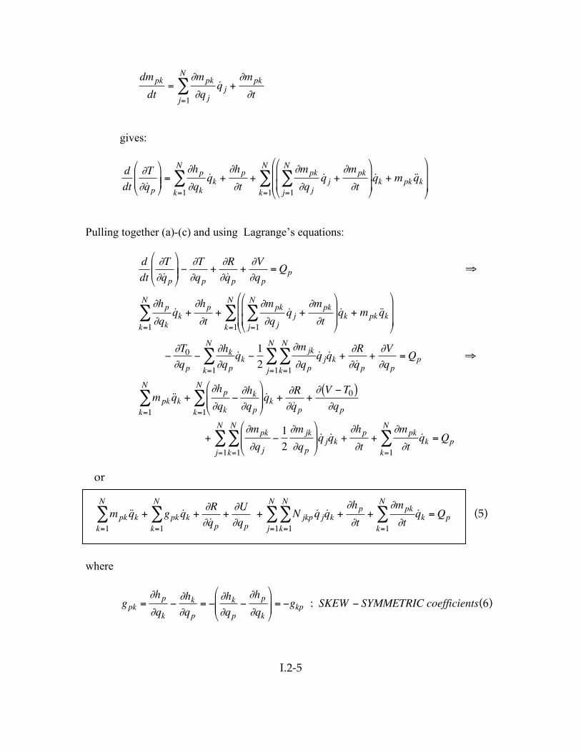
Pulling together (a)-(c) and using Lagrange’s equations:

!

d

dt

"T

" ˙ q p

#

$ % %

&

' ( ( )

"T

"qp

+"R

" ˙ q p+"V

"qp

= Qp *

"hp

"qk

˙ q kk=1

N

+ +"hp

"t+

"mpk

"q j

˙ q jj=1

N

+ +"mpk

"t

#

$

% %

&

'

( ( ˙ q k + m pk ˙ q k

#

$

% %

&

'

( (

k=1

N

+

)"T0

"qp

)"hk

"qp

˙ q kk=1

N

+ )1

2

"m jk

"qp

˙ q j ˙ q kk=1

N

+j=1

N

+ +"R

" ˙ q p+"V

"qp

= Qp *

m pk ˙ q kk=1

N

+ +"hp

"qk

)"hk

"qp

#

$ % %

&

' ( (

k=1

N

+ ˙ q k +"R

" ˙ q p+" V )T0( )"qp

+"mpk

"q j

)1

2

"m jk

"qp

#

$ % %

&

' ( ( ˙ q j ˙ q k

k=1

N

+j=1

N

+ +"hp

"t+

"mpk

"t˙ q k

k=1

N

+ = Qp

or

!

m pk ˙ q kk=1

N

" + gpk

k=1

N

" ˙ q k +#R

# ˙ q p+#U

#qp

+ N jkp ˙ q j ˙ q kk=1

N

"j=1

N

" +#hp

#t+

#mpk

#t˙ q k

k=1

N

" = Qp (5)

where

!

gpk ="hp"qk

#"hk"qp

= #"hk"qp

#"hp"qk

$

% & &

'

( ) ) = #gkp ; SKEW # SYMMETRIC coefficients(6)


I.2-6 ME 564 - Spring 20

!

N jkp ="mpk

"q j#1

2

"m jk

"qp (7)

!

U =V "T0 = "dynamic potential" (8)

Remarks a) Equation (5) represents the most general form of Lagrange’s equations for a system

of particles (we will later extend these to planar motion of rigid bodies). This form of the equations shows the explicit form of the resulting EOM’s.

b) For all systems of interest to us in the course, we will be able to separate the generalized forces

!

Qp in terms of components that are independent and dependent on time. That is we can write:

!

Qp = Pp + f p t( ) where

!

Pp are not explicitly functions of time.

c) A “rheonomic” system is one on which time-dependent position constraints exist are imposed. Otherwise, the system is known as “scleronomic”. We will deal with both rheonomic and scleronomic systems in this course.

d) For many rheonomic systems, the coefficients

!

mpk and

!

gpk will NOT be explicit functions of time. This will be the case for all systems of interest to us in this course. As a result, our EOM’s will be of the form:

!

m pk ˙ q kk=1

N

" + gpk

k=1

N

" ˙ q k +#R

# ˙ q p+#U

#qp


N

"j=1

N

" = Pp + f p t( ) (5a)

e) Note that for a scleronomic system, the position vectors are NOT explicit functions

of time. As a result, equation (1) reduces to:

!

˙ r i ="ri

"q j

˙ q jj=1

N

#

since

!

"ri /"t for a scleronomic system. As a result,

!

T0 = T1 = 0 (see equations (2) and (3)). Consequently, the general form of EOM’s for scleronomic systems reduces to:

!

m pk ˙ q kk=1

N

" +#R

# ˙ q p+#U

#qp


N

"j=1

N

" = Pp + f p t( ) (5b)


I.2-7 ME 564 - Spring 20

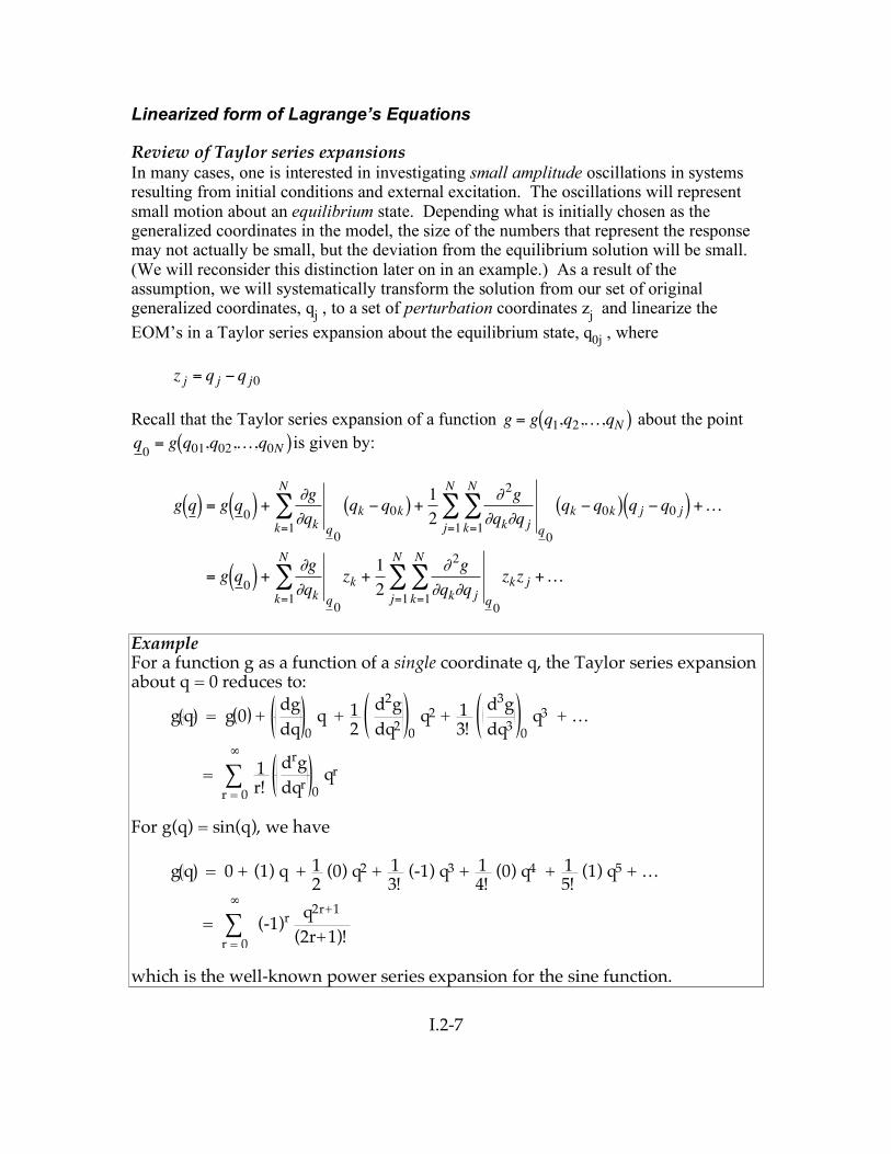
Linearized form of Lagrange’s Equations Review of Taylor series expansions In many cases, one is interested in investigating small amplitude oscillations in systems resulting from initial conditions and external excitation. The oscillations will represent small motion about an equilibrium state. Depending what is initially chosen as the generalized coordinates in the model, the size of the numbers that represent the response may not actually be small, but the deviation from the equilibrium solution will be small. (We will reconsider this distinction later on in an example.) As a result of the assumption, we will systematically transform the solution from our set of original generalized coordinates, qj , to a set of perturbation coordinates zj and linearize the EOM’s in a Taylor series expansion about the equilibrium state, q0j , where

!

z j = q j " q j0 Recall that the Taylor series expansion of a function

!

g = g q1,q2,K,qN( ) about the point

!

q0

= g q01,q02,K,q0N( )is given by:

!

g q( ) = g q0

( ) +"g

"qkk=1

N

#q0

qk $ q0k( ) +1

2

"2g

"qk"q jk=1

N

#q0

qk $ q0k( ) q j $ q0 j( )j=1

N

# +K

= g q0( ) +

"g

"qkk=1

N

#q0

zk +1

2

"2g

"qk"q jk=1

N

#q0

zkz jj=1

N

# +K

Example For a function g as a function of a single coordinate q, the Taylor series expansion about q = 0 reduces to:

g q = g 0 + dg

dq 0 q + 1

2

d2g

dq20 q2 + 1

3!

d3g

dq30 q3 + …

= 1r!

drg

dqr0 qr!

r = 0

!

For g(q) = sin(q), we have g q = 0 + (1) q + 1

2 (0) q2 + 1

3! (-1) q3 + 1

4! (0) q4 + 1

5! (1) q5 + …

= (-1)r q2r+1

(2r+1)!!r = 0

!

which is the well-known power series expansion for the sine function.


I.2-8 ME 564 - Spring 20

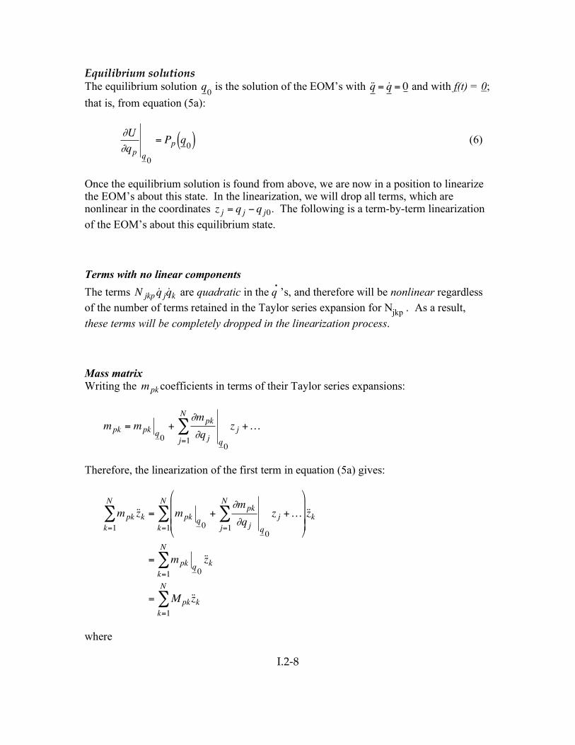
Equilibrium solutions The equilibrium solution

!

q0 is the solution of the EOM’s with

!

˙ q = ˙ q = 0 and with f(t) = 0; that is, from equation (5a):

!

"U

"qpq0

= Pp q0( ) (6)

Once the equilibrium solution is found from above, we are now in a position to linearize the EOM’s about this state. In the linearization, we will drop all terms, which are nonlinear in the coordinates

!

z j = q j " q j0. The following is a term-by-term linearization of the EOM’s about this equilibrium state. Terms with no linear components The terms

!

N jkp ˙ q j ˙ q k are quadratic in the q ’s, and therefore will be nonlinear regardless of the number of terms retained in the Taylor series expansion for Njkp . As a result, these terms will be completely dropped in the linearization process. Mass matrix Writing the

!

mpkcoefficients in terms of their Taylor series expansions:

!

mpk = mpk q0

+"mpk

"q j q0

z jj=1

N

# +K

Therefore, the linearization of the first term in equation (5a) gives:

!

m pk ˙ z kk=1

N

" = m pkq

0

+#mpk

#q jq

0

z j

j=1

N

" +K

$

%

& & &

'

(

) ) ) ˙ z k

k=1

N

"

= m pk q0

˙ z kk=1

N

"

= M pk˙ z kk=1

N

"

where


I.2-9 ME 564 - Spring 20

!

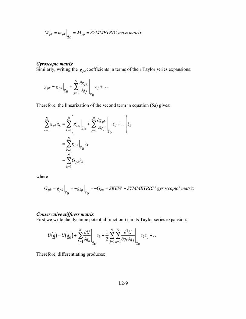
Mpk = mpk q0

= Mkp = SYMMETRIC mass matrix

Gyroscopic matrix Similarly, writing the

!

gpkcoefficients in terms of their Taylor series expansions:

!

gpk = gpk q0

+"gpk

"q j q0

z jj=1

N

# +K

Therefore, the linearization of the second term in equation (5a) gives:

!

gpk ˙ z kk=1

N

" = gpkq

0

+#gpk

#q jq

0

z j

j=1

N

" +K

$

%

& & &

'

(

) ) ) ˙ z k

k=1

N

"

= gpk q0

˙ z kk=1

N

"

= Gpk ˙ z kk=1

N

"

where

!

Gpk = gpk q0

= "gkp q0

= "Gkp = SKEW " SYMMETRIC "gyroscopic" matrix

Conservative stiffness matrix First we write the dynamic potential function U in its Taylor series expansion:

!

U q( ) =U q0( ) +

"U

"qkk=1

N

#q0

zk +1

2

"2U

"qk"q jk=1

N

#q0

zkz jj=1

N

# +K

Therefore, differentiating produces:


I.2-10 ME 564 - Spring 20

!

"U

"qp= 0 +

"U

"qkk=1

N

#q0

"zk"qp

+1

2

"2U

"qk"q jk=1

N

#q0

"zk"qp

z j + zk"z j"qp

$

% & &

'

( ) )

j=1

N

# +K

="U

"qp q0

+1

2

"2U

"qp"q j q0

z jj=1

N

# +1

2

"2U

"qk"qp q0

zkk=1

N

# +K

="U

"qpq0

+1

2Kpj z j

j=1

N

# +1

2Kkp zk

k=1

N

# +K

where

!

Kpj ="2U

"qp"q jq0

= K jp = SYMMETRIC "stiffness matrix"

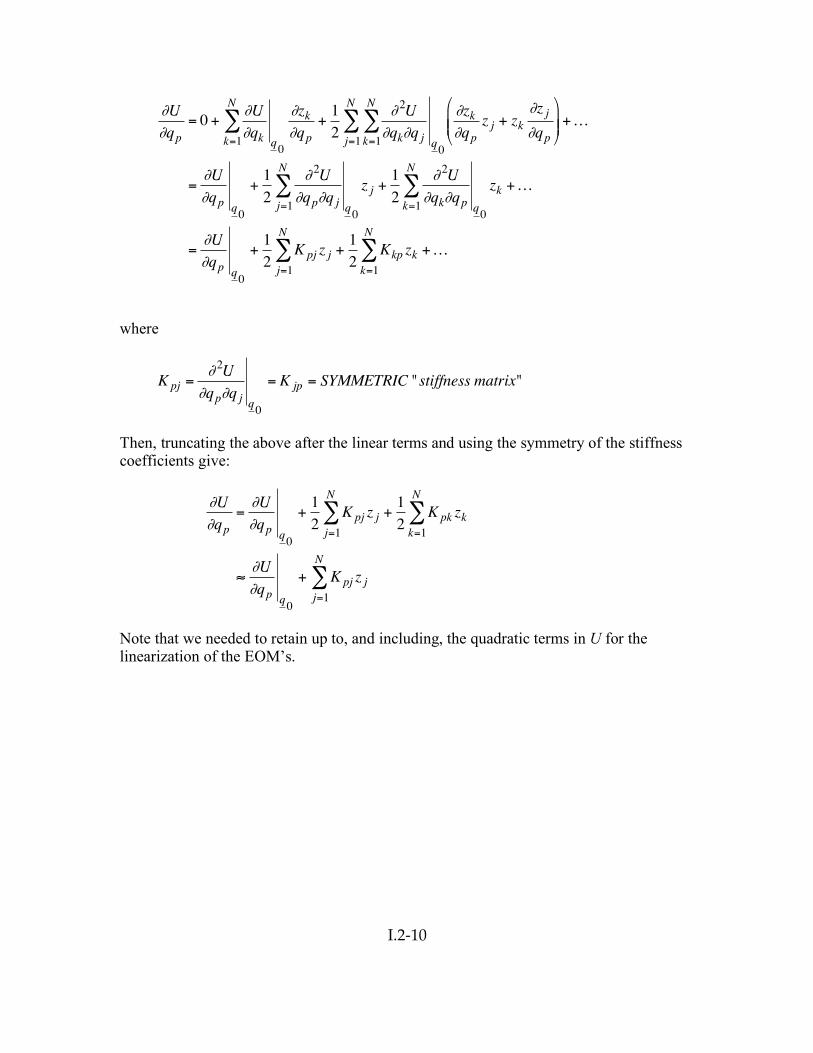
Then, truncating the above after the linear terms and using the symmetry of the stiffness coefficients give:

!

"U

"qp="U

"qpq0

+1

2Kpj z j

j=1

N

# +1

2Kpk zk

k=1

N

#

$"U

"qp q0

+ Kpj z jj=1

N

#

Note that we needed to retain up to, and including, the quadratic terms in U for the linearization of the EOM’s.


I.2-11 ME 564 - Spring 20

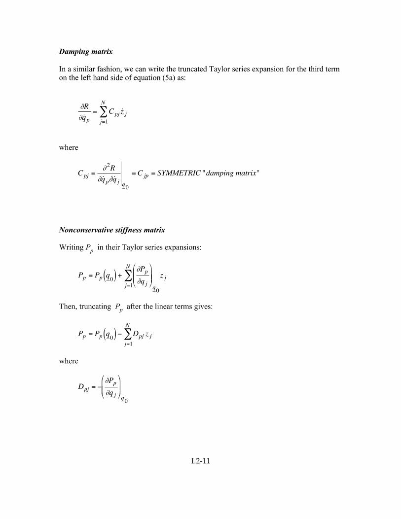
Damping matrix In a similar fashion, we can write the truncated Taylor series expansion for the third term on the left hand side of equation (5a) as:

!

"R

" ˙ q p= Cpj ˙ z j

j=1

N

#

where

!

Cpj ="2

R

" ˙ q p" ˙ q j q0

= C jp = SYMMETRIC "damping matrix"

Nonconservative stiffness matrix Writing Pp in their Taylor series expansions:

!

Pp = Pp q0( ) +"Pp"q j

#

$ % %

&

' ( (

j=1

N

)q0

z j

Then, truncating Pp after the linear terms gives:

!

Pp = Pp q0( ) " Dpj z jj=1

N

#

where

!

Dpj = "#Pp#q j

$

% & &

'

( ) ) q0


I.2-12 ME 564 - Spring 20

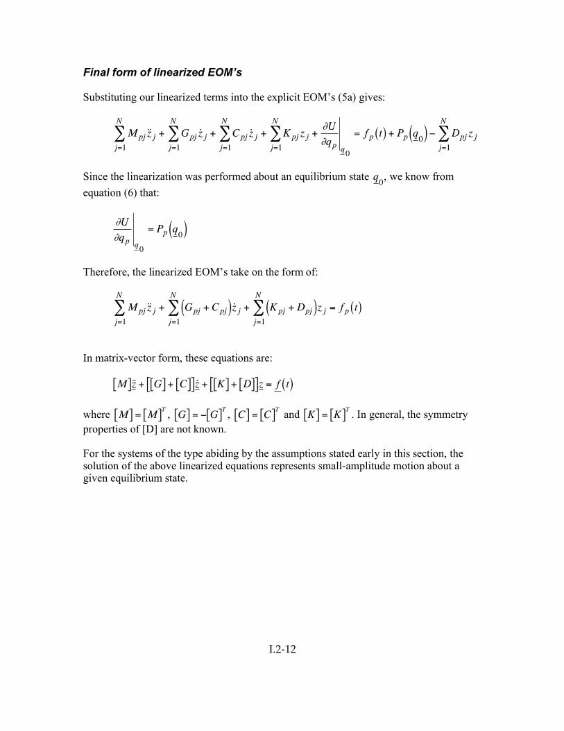
Final form of linearized EOM’s Substituting our linearized terms into the explicit EOM’s (5a) gives:

!

M pj ˙ z jj=1

N

" + Gpj ˙ z jj=1

N

" + Cpj ˙ z jj=1

N

" + K pj z j

j=1

N

" +#U

#qpq

0

= f p t( ) + Pp q0( ) $ Dpj z j

j=1

N

"

Since the linearization was performed about an equilibrium state

!

q0, we know from

equation (6) that:

!

"U

"qpq0

= Pp q0( )

Therefore, the linearized EOM’s take on the form of:

!

M pj ˙ z jj=1

N

" + Gpj + Cpj( ) ˙ z jj=1

N

" + K pj + Dpj( )z j

j=1

N

" = f p t( )

In matrix-vector form, these equations are:

!

M[ ]˙ z + G[ ] + C[ ][ ] ˙ z + K[ ] + D[ ][ ]z = f t( )

where

!

M[ ] = M[ ]T ,

!

G[ ] = " G[ ]T ,

!

C[ ] = C[ ]T and

!

K[ ] = K[ ]T . In general, the symmetry

properties of [D] are not known. For the systems of the type abiding by the assumptions stated early in this section, the solution of the above linearized equations represents small-amplitude motion about a given equilibrium state.


I.2-13 ME 564 - Spring 20

Remarks

(a) The “mass matrix” [M] is always symmetric ( [M] = [M]T ) regardless of the system.

(b) The “gyroscopic matrix” [G] will not appear in the EOM’s for scleronomic systems. To see this, note that the [G] coefficients arise from the hj terms in the T1 portion of the kinetic energy expression. Recall that the appearance of T1 requires the position vectors to be explicit functions of time (that is, for rheonomic systems). However, the [G] matrix may be absent from many rheonomic systems. When it does appear, [G] will be skew-symmetric ( [G] = - [G]T ) . Since [G] is skew-symmetric, there is no power in the term [G] z ; that is, no energy is lost or gained in this term.

(c) The “damping matrix” [C] originates from the non-conservative generalized forces. When the damping forces [C] z are derivable from a Rayleigh dissipation function (as above), the damping matrix will be symmetric and positive semi-definite. With [C] being positive semi-definite, the damping terms [C] z are generally dissipative; that is, energy is lost from the system through these terms.

(d) The matrix [K] is the contribution to the “stiffness matrix” from the dynamic potential function, U = V - T0 and will always be symmetric.

(e) The matrix [D] is the contribution to the stiffness matrix from the non-conservative generalized forces. The symmetry properties of [D] are not known in general. We will therefore assume that [D] will be non-symmetric unless known to be otherwise.

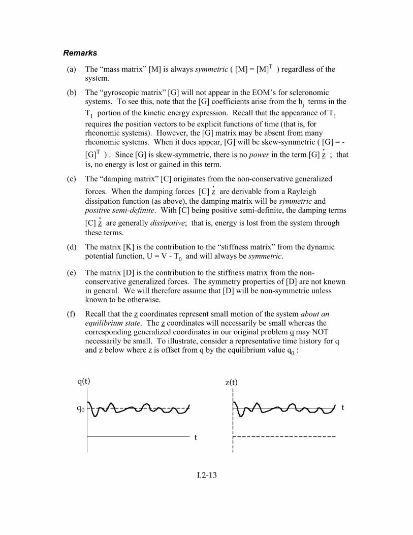
(f) Recall that the z coordinates represent small motion of the system about an equilibrium state. The z coordinates will necessarily be small whereas the corresponding generalized coordinates in our original problem q may NOT necessarily be small. To illustrate, consider a representative time history for q and z below where z is offset from q by the equilibrium value q0 :

q(t)

q0

t

z(t)

t


I.2-14 ME 564 - Spring 20

(g) A set of EOM’s derived for a system via Newton-Euler will be completely equivalent to the above Lagrangian EOM’s, although they may appear to be different in form. In particular, the symmetry/skew-symmetry properties observed above may not be present in the Newton-Euler equations.


I.2-15 ME 564 - Spring 20

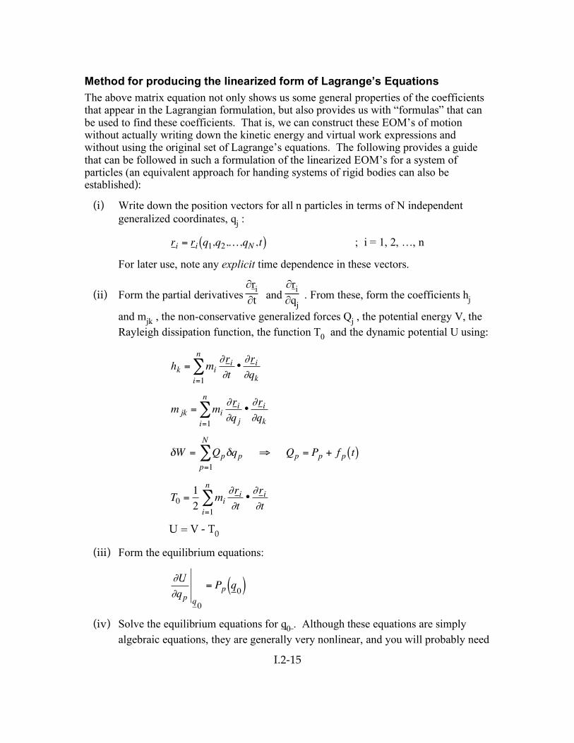
Method for producing the linearized form of Lagrange’s Equations The above matrix equation not only shows us some general properties of the coefficients that appear in the Lagrangian formulation, but also provides us with “formulas” that can be used to find these coefficients. That is, we can construct these EOM’s of motion without actually writing down the kinetic energy and virtual work expressions and without using the original set of Lagrange’s equations. The following provides a guide that can be followed in such a formulation of the linearized EOM’s for a system of particles (an equivalent approach for handing systems of rigid bodies can also be established):

(i) Write down the position vectors for all n particles in terms of N independent generalized coordinates, qj :

!

ri = ri q1,q2,K,qN ,t( ) ; i = 1, 2, …, n

For later use, note any explicit time dependence in these vectors.

(ii) Form the partial derivatives ∂ri∂t and

∂ri∂qj

. From these, form the coefficients hj

and mjk , the non-conservative generalized forces Qj , the potential energy V, the Rayleigh dissipation function, the function T0 and the dynamic potential U using:

!

hk = mi"ri"t

•"ri"qki=1

n

#

!

m jk = mi"ri"q j

•"ri"qki=1

n

#

!

"W = Qp"qp #

p=1

N

$ Qp = Pp + f p t( )

!

T0 =1

2mi

"ri

"t•"r

i

"ti=1

n

#

U = V - T0

(iii) Form the equilibrium equations:

!

"U

"qpq0

= Pp q0( )

(iv) Solve the equilibrium equations for q0 . Although these equations are simply algebraic equations, they are generally very nonlinear, and you will probably need


I.2-16 ME 564 - Spring 20

to solve them numerically. Furthermore, it is likely that more than one equilibrium state may exist and therefore multiple solutions of the equilibrium equations may exist.

(v) Form the mass, gyroscopic, damping and the stiffness matrices:

!

Mpk ="mpk

"q j q0

= Mkp

!

Gpk = gpk q0

= "Gkp

!

Cpk ="2

R

" ˙ q p " ˙ q k

#

$ % %

&

' ( (

q0

= Cpk

!

Kpk ="2U

"qp"qk q0

= Kkp

!

Dpk = "#Pp#qk

$

% &

'

( ) q0

=??

Dkp


I.2-17 ME 564 - Spring 20

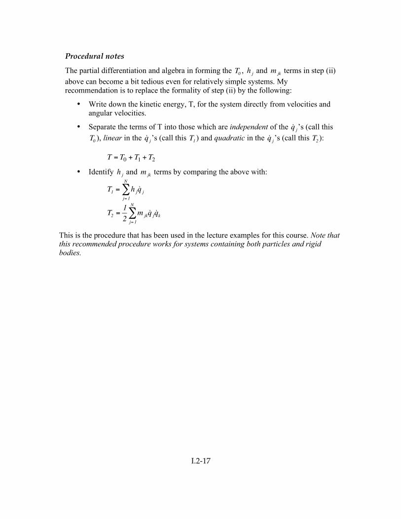
Procedural notes

The partial differentiation and algebra in forming the

!

T0,

!

h j and

!

m jk terms in step (ii) above can become a bit tedious even for relatively simple systems. My recommendation is to replace the formality of step (ii) by the following:

• Write down the kinetic energy, T, for the system directly from velocities and angular velocities.

• Separate the terms of T into those which are independent of the

!

˙ q j’s (call this

!

T0), linear in the

!


!

T1) and quadratic in the

!


!

T2):

!

T = T0 + T1 + T2

• Identify

!

h j and

!

m jk terms by comparing the above with:

!

T1 = h j˙ q j

j= 1

N

"

!

T2 =1

2m jk

˙ q j ˙ q kj= 1

N

"

This is the procedure that has been used in the lecture examples for this course. Note that this recommended procedure works for systems containing both particles and rigid bodies.


I.2-18 ME 564 - Spring 20

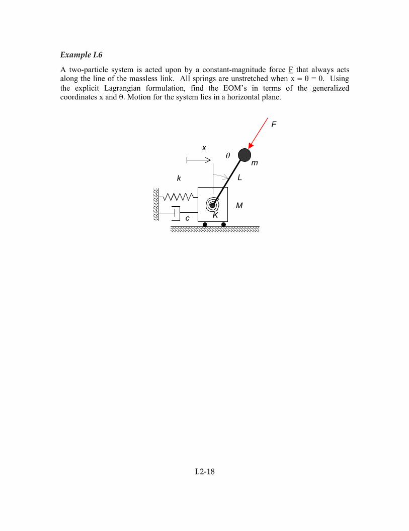
Example I.6

A two-particle system is acted upon by a constant-magnitude force F that always acts along the line of the massless link. All springs are unstretched when x = θ = 0. Using the explicit Lagrangian formulation, find the EOM’s in terms of the generalized coordinates x and θ. Motion for the system lies in a horizontal plane.

c

k

x

M

F

m θ

K

L


I.2-19 ME 564 - Spring 20

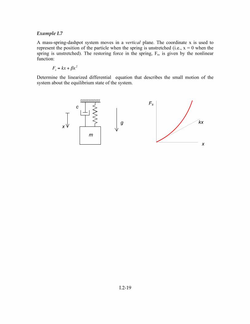
Example I.7

A mass-spring-dashpot system moves in a vertical plane. The coordinate x is used to represent the position of the particle when the spring is unstretched (i.e., x = 0 when the spring is unstretched). The restoring force in the spring, Fs, is given by the nonlinear function:

!

Fs= kx + "x2

Determine the linearized differential equation that describes the small motion of the system about the equilibrium state of the system.

c

g x

m

x

Fs

kx


I.2-20 ME 564 - Spring 20

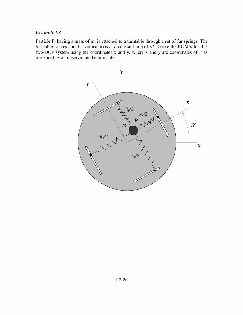
Example I.8

Particle P, having a mass of m, is attached to a turntable through a set of fur springs. The turntable rotates about a vertical axis at a constant rate of Ω. Derive the EOM’s for this two-DOF system using the coordinates x and y, where x and y are coordinates of P as measured by an observer on the turntable.

m

P

ky/2 x

y

X

Y

Ωt

kx/2

ky/2

kx/2


I.2-21 ME 564 - Spring 20

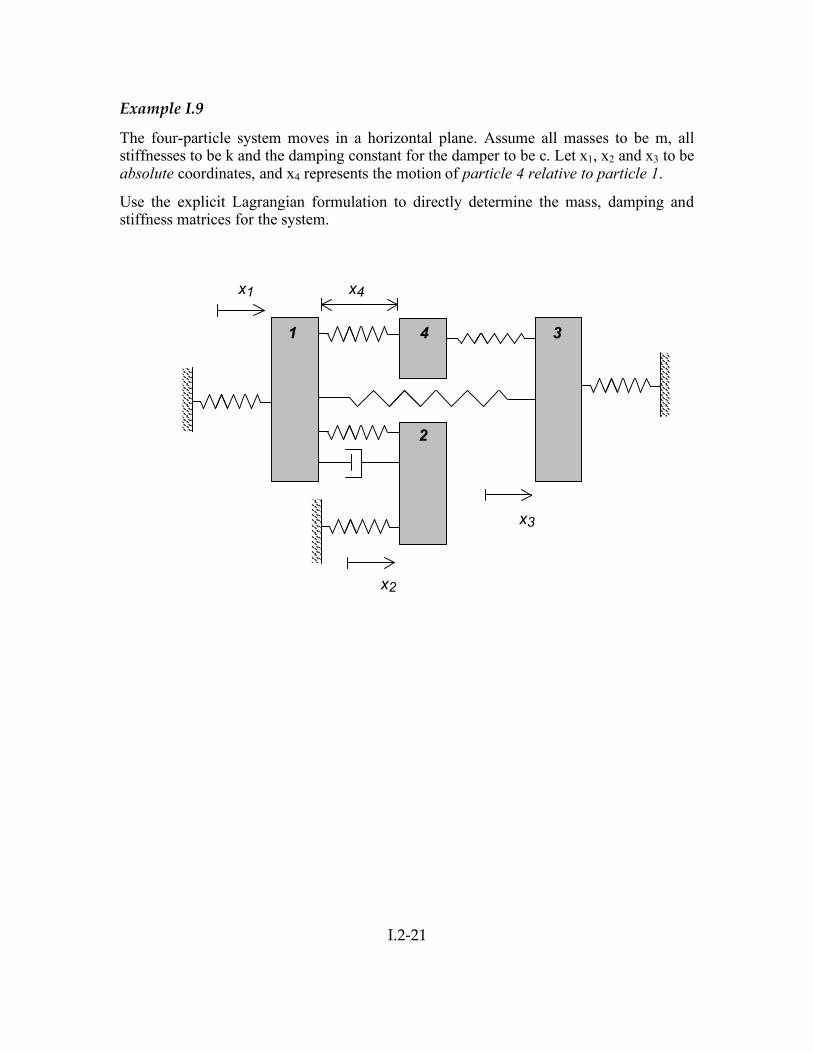
Example I.9

The four-particle system moves in a horizontal plane. Assume all masses to be m, all stiffnesses to be k and the damping constant for the damper to be c. Let x1, x2 and x3 to be absolute coordinates, and x4 represents the motion of particle 4 relative to particle 1.

Use the explicit Lagrangian formulation to directly determine the mass, damping and stiffness matrices for the system.

x1

x2

x3

x4

1 4 3

2

section i.2 lagrange’s equations - linearized eom’slagrange’s equations - linearized eom’s...

Documents