section 9.4 graphical solutions of autonomous equations 553

Section 9.4 Graphical Solutions of Autonomous Equations 553

9. 1 2P has a stable equilibrium at P . 2 2 1 2PdP d P dPdt dt dtœ � œ œ � œ � �"

#

2

2 a b

10. P 1 2P has an unstable equilibrium at P 0 and a stable equilibrium at P .dPdt œ � œ œa b "

#

1 4P P 1 4P 1 2Pd P dPdt dt

2

2 œ � œ � �a b a ba b

11. 2P P 3 has a stable equilibrium at P 0 and an unstable equilibrium at P 3.dPdt œ � œ œa b

2 2P 3 4P 2P 3 P 3d P dPdt dt

2

2 œ � œ � �a b a ba b

Copyright © 2010 Pearson Education, Inc. Publishing as Addison-Wesley.

554 Chapter 9 First-Order Differential Equations

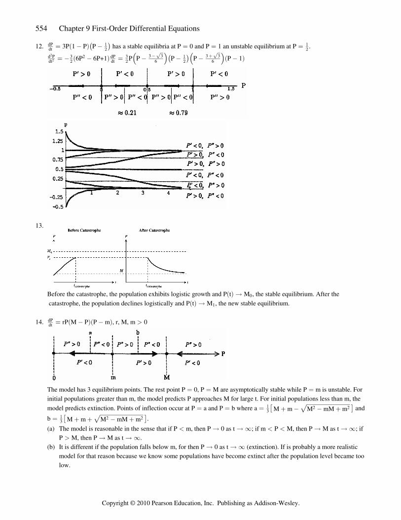
12. 3P 1 P P has a stable equilibria at P 0 and P 1 an unstable equilibrium at P .dPdt œ � � œ œ œa bˆ ‰" "

# #

6P 6P+1 P P P P P 1d P 3 dP 3dt dt 6 6

2 3 3 3 32

2 œ � � œ � � � �# # #� �"a b a bŠ ‹ Š ‹ˆ ‰È È

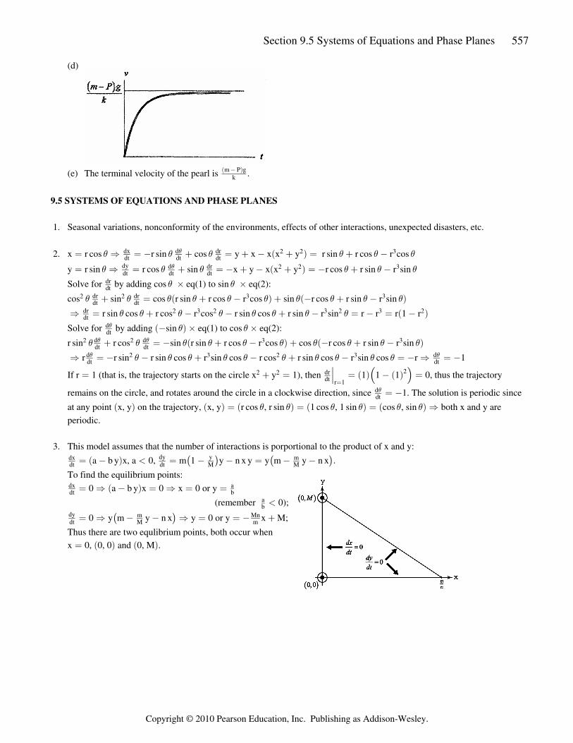
13.

Before the catastrophe, the population exhibits logistic growth and P t M , the stable equilibrium. After thea b Ä 0

catastrophe, the population declines logistically and P t M , the new stable equilibrium.a b Ä 1

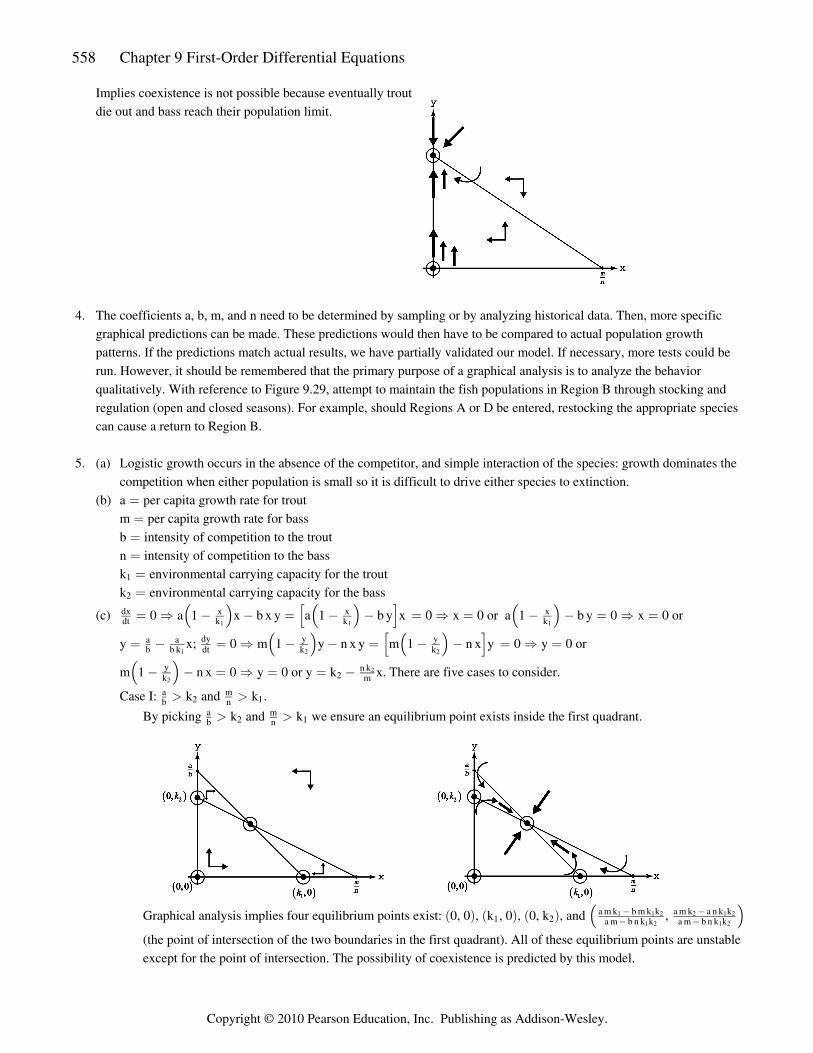
14. rP M P P m , r, M, m 0dPdt œ � � �a ba b

The model has 3 equilibrium points. The rest point P 0, P M are asymptotically stable while P m is unstable. Forœ œ œ

initial populations greater than m, the model predicts P approaches M for large t. For initial populations less than m, the

model predicts extinction. Points of inflection occur at P a and P b where a andM m M mM mœ œ œ � � � �"3

2 2� ‘È b .M m M mM mœ � � � �

"3

2 2� ‘È (a) The model is reasonable in the sense that if P m, then P 0 as t ; if m P M, then P M as t ; if� Ä Ä _ � � Ä Ä _

P M, then P M as t .� Ä Ä _

(b) It is different if the population falls below m, for then P 0 as t (extinction). If is probably a more realisticÄ Ä _

model for that reason because we know some populations have become extinct after the population level became too low.


Section 9.4 Graphical Solutions of Autonomous Equations 555

(c) For P M we see that rP M P P m is negative. Thus the curve is everywhere decreasing. Moreover,� œ � �dPdt a ba b

P M is a solution to the differential equation. Since the equation satisfies the existence and uniqueness conditions,´

solution trajectories cannot cross. Thus, P M as t .Ä Ä _

(d) See the initial discussion above. (e) See the initial discussion above.

15. g v , g, k, m 0 and v t 0dv kdt m

2œ � � a b Equilibrium: g v 0 vdv k

dt m k2 mgœ � œ Ê œ É

Concavity: 2 v 2 v g vd v k dv k kdt m dt m m

22

2 œ � œ � �ˆ ‰ ˆ ‰ˆ ‰ (a)

(b)

(c) v 178.9 122 mphterminal160 ft

0.005 sœ œ œÉ

16. F F Fœ �p r

ma mg k vœ � È g v, v 0 vdv k

dt m 0œ � œÈ a b Thus, 0 implies v , the terminal velocity. If v , the object will fall faster and faster, approaching thedv

dt k kmg mg2 2

0œ œ �ˆ ‰ ˆ ‰ terminal velocity; if v , the object will slow down to the terminal velocity.0

mgk

2� ˆ ‰

17. F F Fœ �p r

ma 50 5 vœ � k k 50 5 vdv 1

dt mœ �a bk k The maximum velocity occurs when 0 or v 10 .dv ft

dt secœ œ

18. (a) The model seems reasonable because the rate of spread of a piece of information, an innovation, or a cultural fad is proportional to the product of the number of individuals who have it (X) and those who do not (N X). When X is�

small, there are only a few individuals to spread the item so the rate of spread is slow. On the other hand, when (N X) is small the rate of spread will be slow because there are only a few indiciduals who can receive it during the�

interval of time. The rate of spread will be fastest when both X and (N X) are large because then there are a lot of�

individuals to spread the item and a lot of individuals to receive it. (b) There is a stable equilibrium at X N and an unstable equilibrium at X 0.œ œ

k N X kX k X N X N 2X inflection points at X 0, X , and X N.d X dX dX Ndt dt dt 2

22

2 œ � � œ � � Ê œ œ œa b a ba b



(c)

(d) The spread rate is most rapid when x . Eventually all of the people will receive the item.œ N2

19. L Ri V i i , V, L, R 0di di V R R Vdt dt L L L R� œ Ê œ � œ � �ˆ ‰

Equilibrium: i 0 idi R V Vdt L R Rœ � œ Ê œˆ ‰

Concavity: id i R di R Vdt L dt L R

22

2 œ � œ � �ˆ ‰ ˆ ‰ ˆ ‰ Phase Line:

If the switch is closed at t 0, then i 0 0, and the graph of the solution looks like this:œ œa b

As t , it i . (In the steady state condition, the self-inductance acts like a simple wire connector and, asÄ _ Ä œsteady stateVR

a result, the current throught the resistor can be calculated using the familiar version of Ohm's Law.)

20. (a) Free body diagram of the pearl:

(b) Use Newton's Second Law, summing forces in the direction of the acceleration:

mg Pg kv ma g v.� � œ Ê œ �dv m P kdt m m

ˆ ‰�

(c) Equilibrium: v 0dv kdt m k

m P gœ � œŠ ‹a b�

vÊ œterminalm P g

ka b�

Concavity: vd v k dv kdt m dt m k

2 m P g2

2 œ � œ � �ˆ ‰ Š ‹a b�


Section 9.5 Systems of Equations and Phase Planes 557

(d)

(e) The terminal velocity of the pearl is .a bm P gk�

9.5 SYSTEMS OF EQUATIONS AND PHASE PLANES

1. Seasonal variations, nonconformity of the environments, effects of other interactions, unexpected disasters, etc.

2. x r cos r sin cos y x x x y r sin r cos r cosœ Ê œ � � œ � � � œ � �) ) ) ) ) )dx d drdt dt dt

2 2 3) a b y r sin r cos sin x y x x y r cos r sin r sinœ Ê œ � œ � � � � œ � � �) ) ) ) ) )

dydt dt dt

d dr 2 2 3) a b Solve for by adding cos eq(1) to sin eq(2):dr

dt ) )‚ ‚

cos sin cos r sin r cos r cos sin r cos r sin r sin2 2 3 3dr drdt dt) ) ) ) ) ) ) ) ) )� œ � � � � � �a b a b

r sin cos r cos r cos r sin cos r sin r sin r r r 1 rÊ œ � � � � � œ � œ �drdt

2 3 2 3 2 3 2) ) ) ) ) ) ) ) a b

Solve for by adding sin eq(1) to cos eq(2):ddt) a b� ‚ ‚) )

r sin r cos sin r sin r cos r cos cos r cos r sin r sin2 2 3 3d ddt dt) ) ) ) ) ) ) ) ) )) )� œ � � � � � � �a b a b

r r sin r sin cos r sin cos r cos r sin cos r sin cos r 1Ê œ � � � � � � œ � Ê œ �d ddt dt

2 3 2 3) )) ) ) ) ) ) ) ) ) )

If r 1 (that is, the trajectory starts on the circle x y 1), then 1 1 1 0, thus the trajectoryœ � œ œ � œ2 2 drdt r 1

2¹ a b a bŠ ‹œ

remains on the circle, and rotates around the circle in a clockwise direction, since 1. The solution is periodic sinceddt) œ �

at any point x, y on the trajectory, x, y r cos , r sin 1 cos , 1 sin cos , sin both x and y area b a b a b a b a bœ œ œ Ê) ) ) ) ) )

periodic.

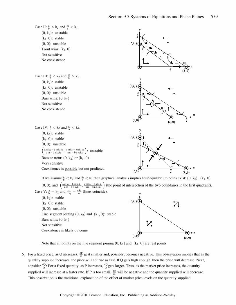
3. This model assumes that the number of interactions is porportional to the product of x and y:

a b y x, a 0, m 1 y n x y y m y n xdx mdt dt M M

dy yœ � � œ � � œ � � Þa b ˆ ‰ ˆ ‰ To find the equilibrium points:

0 a b y x 0 x 0 or ydx adt bœ Ê � œ Ê œ œa b

(remember 0);ab �

0 y m y n x y 0 or y x M;dydt M m

m Mnœ Ê � � Ê œ œ � �ˆ ‰ Thus there are two equlibrium points, both occur when x 0, 0, 0 and 0, M .œ a b a b



Implies coexistence is not possible because eventually trout die out and bass reach their population limit.

4. The coefficients a, b, m, and n need to be determined by sampling or by analyzing historical data. Then, more specific graphical predictions can be made. These predictions would then have to be compared to actual population growth patterns. If the predictions match actual results, we have partially validated our model. If necessary, more tests could be run. However, it should be remembered that the primary purpose of a graphical analysis is to analyze the behavior qualitatively. With reference to Figure 9.29, attempt to maintain the fish populations in Region B through stocking and regulation (open and closed seasons). For example, should Regions A or D be entered, restocking the appropriate species can cause a return to Region B.

5. (a) Logistic growth occurs in the absence of the competitor, and simple interaction of the species: growth dominates the competition when either population is small so it is difficult to drive either species to extinction. (b) a per capita growth rate for troutœ

m per capita growth rate for bassœ

b intensity of competition to the troutœ

n intensity of competition to the bassœ

k environmental carrying capacity for the trout1 œ

k environmental carrying capacity for the bass2 œ

(c) 0 a 1 x b x y a 1 b y x 0 x 0 or a 1 b y 0 x 0 ordx x x xdt k k kœ Ê � � œ � � œ Ê œ � � œ Ê œŠ ‹ Š ‹ Š ‹’ “

1 1 1

y x; 0 m 1 y n x y m 1 n x y 0 y 0 orœ � œ Ê � � œ � � œ Ê œa ab b k dt k k

dy y y1 2 2

Š ‹ Š ‹’ “ m 1 n x 0 y 0 or y k x. There are five cases to consider.Š ‹� � œ Ê œ œ �y

k m2n k

2

2

Case I: k and k .a mb n2 1� �

By picking k and k we ensure an equilibrium point exists inside the first quadrant.a mb n2 1� �

Graphical analysis implies four equilibrium points exist: 0, 0 , k , 0 , 0, k , and , a b a b a b Š ‹1 2a m k b m k k a m k a n k

a m b n k k1 1 2 2

1 2

� ��

1 2

1 2

ka m b n k k�

(the point of intersection of the two boundaries in the first quadrant). All of these equilibrium points are unstable except for the point of intersection. The possibility of coexistence is predicted by this model.



Case II: k and k .a mb n2 1� �

0, k : unstablea b2

k , 0 : stablea b1

0, 0 : unstablea b Trout wins: k , 0a b1

Not sensitive No coexistence

Case III: k and k .a mb n2 1� �

0, k : stablea b2

k , 0 : unstablea b1

0, 0 : unstablea b Bass wins: 0, ka b2

Not sensitive No coexistence

Case IV: k and k .a mb n2 1� �

0, k : stablea b2

k , 0 : stablea b1

0, 0 : unstablea b , : unstableŠ ‹a m k b m k k a m k a n k k

a m b n k k a m b n k k1 1 2 2 1 2

1 2 1 2

� ��

Bass or trout: 0, k or k , 0a b a b2 1

Very sensitive Coexistence is but not predictedpossible

If we assume k and k then graphical analysis implies four equilibrium poins exist: 0, k , k , 0 ,a mb n2 1 2 1� � a b a b

0, 0 , and , (the point of intersection of the two boundaries in the first a b Š ‹a m k b m k k a m k a n k ka m b n k k a m b n k k

1 1 2 2 1 2

1 2 1 2

� �� quadrant).

Case V: k and (lines coincide).a ab b k m2

n kœ œ1

2

0, k : stablea b2

k , 0 : stablea b1

0, 0 : unstablea b Line segment joining 0, k and k , 0 : stablea b a b2 1

Bass wins: 0, ka b2

Not sensitive Coexistence is likely outcome

Note that all points on the line segment joining 0, k and k , 0 are rest points.a b a b2 1

6. For a fixed price, as Q increases, gest smaller and, possibly, becomes negative. This observation implies that as thedPdt

quantity supplied increases, the price will not rise as fast. If Q gets high enough, then the price will decrease. Next,

consider : For a fixed quantity, as P increases, gets larger. Thus, as the market price increases, the quantitydQ dQdt dt

supplied will increase at a faster rate. If P is too small, will be negative and the quantity supplied will decrease.dQdt

This observation is the traditional explanation of the effect of market price levels on the quantity supplied.



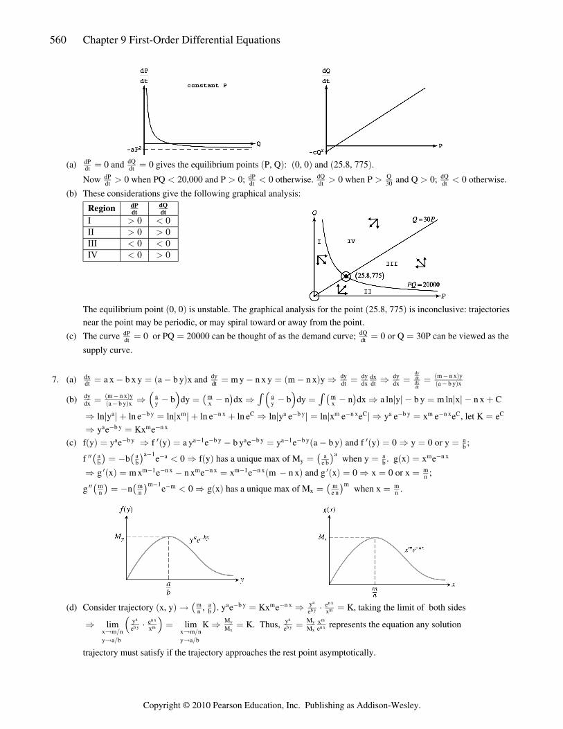
(a) 0 and 0 gives the equilibrium points P, Q : 0, 0 and 25.8, 775 .dPdt dt

dQœ œ a b a b a b Now 0 when PQ 20,000 and P 0; 0 otherwise. 0 when P and Q 0; 0 otherwise.dP dP

dt dt dt 30 dtdQ Q dQ� � � � � � � �

(b) These considerations give the following graphical analysis:

I 0 0II 0 0III 0 0IV 0 0

Region dPdt dt

dQ

� ��

The equilibrium point 0, 0 is unstable. The graphical analysis for the point 25.8, 775 is inconclusive: trajectoriesa b a b near the point may be periodic, or may spiral toward or away from the point.

(c) The curve 0 or PQ 20000 can be thought of as the demand curve; 0 or Q 30P can be viewed as thedPdt dt

dQœ œ œ œ

supply curve.

7. (a) a x b x y a b y x and m y n x y m n x ydx dxdt dt dt dx dt dx a b y x

dy dy dy dy m n x yœ � œ � œ � œ � Ê œ Ê œ œa b a b dydtdxdt

a ba b

��

(b) b dy n dx b dy n dx a ln y b y m ln x n x Cdydx a b y x y x y x

m n x y a m a mœ Ê � œ � Ê � œ � Ê l l � œ l l � �a ba b

�� Š ‹ Š ‹ˆ ‰ ˆ ‰' '

ln y ln e ln x ln e ln e ln y e ln x e e y e x e e , let K eÊ l l � œ l l � � Ê l l œ l l Ê œ œa b y m n x C a b y m n x C a b y m n x C C� � � � � �

y e Kx eÊ œa b y m n x� �

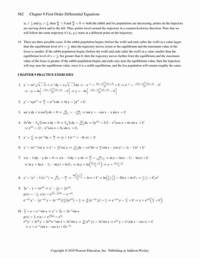
(c) f y y e f y a y e b y e y e a b y and f y 0 y 0 or y ;a b a b a b a bœ Ê œ � œ � œ Ê œ œa b y a 1 b y a b y a 1 b y ab

� w � � � � � w

f b e 0 f y has a unique max of M when y . g x x eww � ��ˆ ‰ ˆ ‰ ˆ ‰a b a ba a a ab b e b b

a 1 aa m n xyœ � � Ê œ œ œ

g x m x e n x e x e m n x and g x 0 x 0 or x ;Ê œ � œ � œ Ê œ œw � � � � � wa b a b a bm 1 n x m n x m 1 n x mn

g n e 0 g x has a unique max of M when x .ww ��ˆ ‰ ˆ ‰ ˆ ‰a bm m m mn n e n n

m 1 mmxœ � � Ê œ œ

(d) Consider trajectory x, y , . y e Kx e K, taking the limit of both sidesa b ˆ ‰Ä œ Ê † œm a en b x

a b y m n x ye

� �a

b y

n x

m

K K. Thus, represents the equation any solutionÊ † œ Ê œ œlim limx m n x m ny a b y a b

y ye e

e xx M M e

M M

Ä Î Ä Î

Ä Î Ä Î

Š ‹a a

b y b y

n x m

m n xy y

x x

trajectory must satisfy if the trajectory approaches the rest point asymptotically.



(e) Pick initial condition y . Then, from the figure at0ab�

right, f y M implies M and thusa b0 y yMM e

x ye

� œ �y

x

m

n x0a

b y0

M . From the figure for g x , there exists axe x

m

n x � a b unique x satisfying M . That is, for each0 x

m xn e� �

m

n x

y there is a unique x satisfying . Thus,� œa xb M e

ye

Ma

b yy

x

m

n x

there can exist only one trajectory solution approaching

, . (You can think of the point x , y as the initialˆ ‰ a bm an b 0 0

condition for that trajectory.)

(f) Likewise there exists a unique trajectory when y . Again, f y M implies M and thus0 0 y ya xb M e

M ye

� � œ �a b y

x

m

n x0a

b y0

M . From the figure for g x , there exists a unique x satisfying M . That is, for each y there isx m x ae n e bx 0 x

m m

n x n x� � � �a b a unique x satisfying . Thus, there can exist only one trajectory solution approaching , .y

eMM e n b

x m aa

b yy

x

m

n xœ ˆ ‰

8. Let z y z y , then given the differential equation y F x, y, y , we can write it as the followingœ œ Ê œ œ œw w ww ww wdydx dx

dz a b system of first order differential equations: zdy

dx œ

F x, y, zdzdx œ a b

In general, for the n order differential equation given by y F x, y, y , y , . . ., y , let z yth n n 11

dydx

a b a bœ œ œˆ ‰w ww � w

z y , let z z y , z y , . . ., let z z y z y . This gives us theÊ œ œ œ œ Ê œ œ œ œ Ê œdz dzdx dx1 1 2 n 2 n 12 n 1

n 1 n1 2w ww w ww w www w � w� � �

a b a b

following system of first order differential equations: zdydx 1œ

z dzdx 2

1 œ

z dzdx 3

2 œ

ã

z dzdx n 1n 2� œ �

F x, y, z , z , . . ., z dzdx 1 2n 1� œ a bn 1�

9. In the absence of foxes b 0 a x and the population of rabbits grows at a rate proportional to the number ofÊ œ Ê œdxdt

rabbits.

10. In the absence of rabbits d 0 c y and the population of foxes decays (since the foxes have no food source)Ê œ Ê œ �dydt

at a rate proportional to the number of foxes.

11. a b y x 0 y or x 0; c d x y 0 x or y 0 equilibrium points at 0, 0 ordx a cdt b dt d

dyœ � œ Ê œ œ œ � � œ Ê œ œ Êa b a b a b , . For the point 0, 0 , there are no rabbits and no foxes. It is an unstable equilibrium point, if there are no foxes, ˆ ‰ a bc a

d b but

a few rabbits are introduced, then a the rabbit population will grow exponentially away from 0, 0dxdt œ Ê a b

12. Let x t and y t both be positive and suppose that they satisfy the differential equations a b y x anda b a b a bdxdt œ �

c d x y. Let C t a ln y t b y t d x t c ln x t C t a b y t d x t cdydt y t x t

y t x tœ � � œ � � � Ê œ � � �a b a b a b a b a b a b a b a b a bw w ww wa b a ba b a b

b y t d x t b c d x t x t d a b y t y t 0œ � � � œ � � � � � � œŠ ‹ Š ‹ Š ‹ Š ‹a b a b a b a b a b a ba b a ba c a cy t x t y t x ta b a b a b a b

w w

Since C t 0 C t constant.wa b a bœ Ê œ

13. Consider a particular trajectory and suppose that x , y is such that x and y , then 0 and 0 thea b0 0 0 0c a dxd b dt dt

dy� � � � Ê

rabbit population is increasing while the fox population is decreasing, points on the trajectory are moving down and to the

right; if x and y , then 0 and 0 both the rabbit and fox populations are increasing, points on the0 0c a dxd b dt dt

dy� � � � Ê

trajectory are moving up and to the right; if x and y , then 0 and 0 the rabbit population is0 0c a dxd b dt dt

dy� � � � Ê

decreasing while the fox population is increasing, points on the trajectory are moving up and to the left; and finally if



x and y , then 0 and 0 both the rabbit and fox populations are decreasing, points on the trajectory0 0c a dxd b dt dt

dy� � � � Ê

are moving down and to the left. Thus, points travel around the trajectory in a counterclockwise direction. Note that we will follow the same trajectory if x , y starts at a different point on the trajectory.a b0 0

14. There are three possible cases: If the rabbit population begins (before the wolf) and ends (after the wolf) at a value larger than the equilibrium level of x , then the trajectory moves closer to the equilibrium and the maximum value of theœ c

d

foxes is smaller. If the rabbit population begins (before the wolf) and ends (after the wolf) at a value smaller than the equilibrium level of x , but greater than 0, then the trajectory moves further from the equilibrium and the maximumœ c

d

value of the foxes is greater. If the rabbit population begins and ends very near the equilibrium value, then the trajectory will stay near the equilibrium value, since it is a stable equilibrium, and the fox population will remain roughly the same.

CHAPTER 9 PRACTICE EXERCISES

1. y xe x 2 e dy x x 2 dx e C e Cw � � �� œ � Ê œ � Ê � œ � Ê œ �y y y y2 x 2 3x 4 2 x 2 3x 415 15

È È a b a b a b a b3/2 3/2

y ln C y ln CÊ � œ � Ê œ � �’ “ ’ “� � � � � �2 x 2 3x 4 2 x 2 3x 415 15

a b a b a b a b3/2 3/2

2. y xye e x dx ln y e Cw "#œ Ê œ Ê œ �x x xdy

y2 2 2

3. sec x dy x cos y dx 0 tan y cos x x sin x C� œ Ê œ � Ê œ � � �2 dycos y sec x

x dx2

4. 2x dx 3 y csc x dy 0 3 y dy dx 2y 2 2 x cos x 4x sin x C2 3/2 22xcsc x� œ Ê œ Ê œ � � �È È a b2

y 2 x cos x 2x sin x CÊ œ � � �3/2 21a b

5. y ye dy y 1 e ln x Cw � �œ Ê œ Ê � œ � �e dxxy x

y yy a b k k

6. y xe csc y y csc y dy x e dx sin y cos y x 1 e Cw � wœ Ê œ Ê œ Ê � œ � �x y x xx e e ee csc y 2

x y y

y a b a b

7. x x 1 dy y dx 0 x x 1 dy y dx ln y ln x 1 ln x Ca b a b a b a b� � œ Ê � œ Ê œ Ê œ � � �dyy x x 1

dxa b�

ln y ln x 1 ln x ln C ln y ln yÊ œ � � � Ê œ Ê œa b a b Š ‹1C x 1 C x 1

x x1 1a b a b� �

8. y y 1 x ln x C ln 2ln x ln C C xw ��

� �œ � Ê œ Ê œ � Ê œ � Ê œa ba b Š ‹2 1 2dy y 1 y 1y 1 x 2 y 1 y 1

dx1 12

lnŠ ‹y 1y 1�

�

9. 2y y xe y y e .w w "#� œ Ê � œx/2 x/2x

2

p x , v x e e .a b a bœ � œ œ"#

�' ˆ ‰�

"

#dx x/2

e y e y e e e y e y C y e C� w � � � �"#

x/2 x/2 x/2 x/2 x/2 x/2 x/2x x d x x x2 2 dx 2 4 4� œ œ Ê œ Ê œ � Ê œ �ˆ ‰ˆ ‰ˆ ‰ ˆ ‰ Š ‹2 2

10. y e sin x y 2y 2e sin x.y2

x xw

� œ Ê � œ� w �

p x 2, v x e e .a b a bœ œ œ' 2dx 2x

e y 2e y 2e e sin x 2e sin x e y 2e sin x e y e sin x cos x C2x 2x 2x x x 2x x 2x xddx

w �� œ œ Ê œ Ê œ � �a b a b y e sin x cos x CeÊ œ � �� x 2xa b


Chapter 9 Practice Exercises 563

11. xy 2y 1 x y y .w � w� œ � Ê � œ �1 2 1 1x x x

ˆ ‰ 2

v x e e e x .a b œ œ œ œ2 2ln x ln x 2' dxx

2

x y 2xy x 1 x y x 1 x y x C y2 2 2d x 1 Cdx 2 x x

w "#� œ � Ê œ � Ê œ � � Ê œ � �a b 2

2

12. xy y 2x ln x y y 2 ln x.w w� œ Ê � œˆ ‰1x

v x e e . y y ln xa b ˆ ‰ ˆ ‰œ œ œ � œ Ê� � w' dxx ln x 1 1 1 2

x x x x2

y ln x y C y x Cxln x ln xd 1 2 1dx x x x

2 2ˆ ‰ c d c d† œ Ê † œ � Ê œ �

13. 1 e dy ye e dx 0 1 e y e y e y y .a b a b a b� � � œ Ê � � œ � Ê œ œx x x x x x e e1 e 1 e

� w � w� �

�x x

x x

�

a b

v x e e e 1.a b œ œ œ �' e dxx

1 ex xa b� ln e 1 xa b�

e 1 y e 1 y e 1 e e 1 y e Ce 1 ya b a b a b c d a bˆ ‰ a bx x x x x xe e d1 e 1 e dx

x� � � œ � Ê œ � Ê � œ ��w � ��

�x x

x x

�

a b

yÊ œ œe C e Ce 1 1 e

� �x x

x x� ��

14. e dy e y 4x dx 0 y 4x e p x 1, v x e e e y e 4x e� �x x x dx x x x 2xdy dydx dx� � œ Ê � œ Ê œ œ œ Ê � œa b a b a b ' 1

y e 4x e y e 4x e dx y e 2x e e C y 2x e e C eÊ œ Ê œ Ê œ � � Ê œ � �ddx

x 2x x 2x x 2x 2x x x xa b ' �

15. x 3y dy y dx 0 x dy y dx 3y dy xy 3y dy xy y Ca b a b� � œ Ê � œ � Ê œ � Ê œ � �2 2 2 3ddx

16. x dy 3y x cos x dx 0 y y x cos x. Let v y e e e x .� � œ Ê � œ œ œ œ œa b a bˆ ‰� w �2 3 3ln x ln x 33x

' 3dxx

3

Then x y 3x y cos x and x y cos x dx sin x C. So y x sin x C3 2 3 3w �� œ œ œ � œ �' a b

17. x 1 2y x y y . Let v x e e e x 1 .a b a b a bˆ ‰� � œ Ê � œ œ œ œ œ �dydx x 1 x 1

2 x dx 2ln x 1 ln x 1 2w � ��

' 2x 1

2�

a b a b

So y x 1 x 1 y x 1 x x 1 y x 1 x x 1 dxy x 1w� �a b a b a b a b a b a b� ‘a b� � � œ � Ê œ � Ê � œ ��

2 2 2 22 x dx 1 x 1 dx

2a b a b

' y x 1 C y x 1 C . We have y 0 1 1 C. SoÊ � œ � � Ê œ � � � œ Ê œa b a b a bŠ ‹2 2x x x x

3 2 3 2

3 2 3 2�

y x 1 1œ � � �a b Š ‹�2 x x3 2

3 2

18. x 2y x 1 y y x . Let v x e e x . So x y 2xy x xdydx x x

2 ln x 2 2 32 1 dx� œ � Ê � œ � œ œ œ � œ �w wˆ ‰ a b ' ˆ ‰2x

2

x y x x x y C y . We have y 1 1 1 C C .Ê œ � Ê œ � � Ê œ � � œ Ê œ � � Ê œd x x x C 1 1dx 4 2 4 x 4 4

2 3 2a b a b4 2 2

2" "# #

So y œ � � œx 1 x 2x 14 4x 4x

2 4 2

2 2" � �#

19. 3x y x . Let v x e e . So e y 3x e y x e e y x e e y e C.dydx dx 3

2 2 3x dx x x 2 x 2 x x 2 x x xd 1� œ œ œ � œ Ê œ Ê œ �a b Š ‹' 2 3 3 3 3 3 3 3 3w

We have y 0 1 e 1 e C 1 C C and e y e y ea b a bœ � Ê � œ � Ê � œ � Ê œ � œ � Ê œ �0 0 x x x1 1 4 1 4 1 43 3 3 3 3 3 3

3 3 3 3 3�

20. xdy y cos x dx 0 xy y cos x 0 y y . Let v x e e x.� � œ Ê � � œ Ê � œ œ œ œa b a bˆ ‰w w 1 cos xx x

dx ln x' 1x

So xy x y cos x xy cos x xy cos x dx xy sin x C. We have y 0 0 1 Cw � œ Ê œ Ê œ Ê œ � œ Ê œ �ˆ ‰ ˆ ‰ ˆ ‰a b1 dx dx 2 2

' 1 1

C 1. So xy 1 sin x yÊ œ � œ � � Ê œ � �1 sin xx

21. xy x 2 y 3x e y y 3x e . Let v x e e . Sow � w � �� œ Ê � œ œ œ œa b a bˆ ‰3 x 2 x dx x 2ln xx 2 ex x

' ˆ ‰x 2x

x

2

�

y y 3 y 3 y 3x C. We have y 1 0 0 3 1 C C 3e e x 2 d e ex x x dx x x

x x x x

2 2 2 2w �� œ Ê † œ Ê † œ � œ Ê œ � Ê œ �ˆ ‰ ˆ ‰ a b a b

y 3x 3 y x e 3x 3Ê † œ � Ê œ �ex

2 xx

2� a b



22. y dx 3x xy 2 dy 0 0 x 1 x .� � � œ Ê � œ Ê � � œ � Ê � � œ �a b Š ‹dx dx 3x 2 dx 3 2dy y dy y y dy y y

3x xy 2� �

P y 1 P y dy 3ln y y v y e y ea b a b a bœ � Ê œ � Ê œ œ3y

3ln y y 3 y' � �

y e x y e 1 x 2y e y e x 2y e dy 2e y 2y 2 C3 y 3 y 2 y 3 y 2 y y 23y

� w � � � � �� œ � Ê œ � œ � � �Š ‹ a b' y . We have y 2 1 1 C 4e andÊ œ œ � Ê � œ Ê œ �3 2 y 2y 2 Ce

x 22 1 2 2 Ceˆ ‰ a b2 y 1� � � � � �a b �

yÊ œ3 2 y 2y 2 4ex

ˆ ‰2 y 1� � � �

23. To find the approximate values let y y y cos x 0.1 with x 0, y 0, and 20 steps. Use an n 1 n 1 n 1 0 0œ � � œ œ� � �a ba b spreadsheet, graphing calculator, or CAS to obtain the values in the following table.

x y 0 00.1 0.10000.2 0.20950.3 0.32850.4 0.45680.5 0.59460.6 0.74180.7 0.89860.8 1.06490.9 1.24111.0 1.4273

x y 1.1 1.62411.2 1.83191.3 2.05131.4 2.28321.5 2.52851.6 2.78841.7 3.06431.8 3.35791.9 3.67092.0 4.0057

24. To find the approximate values let y y 2 y 2x 3 0.1 with x 3, y 1, and 20 steps. Use an n 1 n 1 n 1 0 0œ � � � œ � œ� � �a ba ba b spreadsheet, graphing calculator, or CAS to obtain the values in the following table.

x y 3.0 1.00002.9 0.70002.8 0.33602.7 0.09662.6 0.59982.5 1.17182.4 1.80622.3 2.49132.2 3.

�� 2099

2.1 3.93932.0 4.6520

x y 1.9 5.31721.8 5.90261.7 6.37681.6 6.71191.5 6.88611.4 6.88611.3 6.7084

� ��

� ��

1.2 6.36011.1 5.85851.0 5.2298

25. To estimate y 3 , let y y 0.05 with initial values x 0, y 1, and 60 steps. Use a spreadsheet,a b a bŠ ‹œ � œ œn 1 0 0x 2y

x 1��

n 1 n 1

n 1

� �

�

graphing calculator, or CAS to obtain y 3 0.8981.a b ¸

26. To estimate y 4 , let z y 0.05 with initial values x 1, y 1, and 60 steps. Use aa b a bŠ ‹n n 1 0 0x 2y 1

xœ � œ œ�� 2

n 1 n 1

n 1

�

�

�

spreadsheet, graphing calculator, or CAS to obtain y 4 4.4974.a b ¸27. Let y y dx with starting values x 0 and y 2, and steps of 0.1 and 0.1. Use a spreadsheet,n n 1 0 0

1eœ � œ œ �� ˆ ‰a bx y 2n 1 n 1� �

� �

programmable calculator, or CAS to generate the following graphs. (a)


Chapter 9 Practice Exercises 565

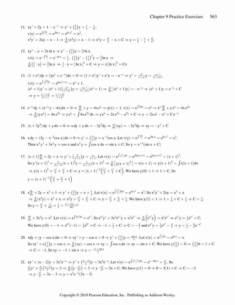
(b) Note that we choose a small interval of x-values because the y-values decrease very rapidly and our calculator cannot handle the calculations for x 1. (This occurs because the analytic solution is y 2 ln 2 e , which has anŸ � œ � � �a b�x

asymptote at x ln 2 0.69. Obviously, the Euler approximations are misleading for x 0.7.)œ � ¸ Ÿ �

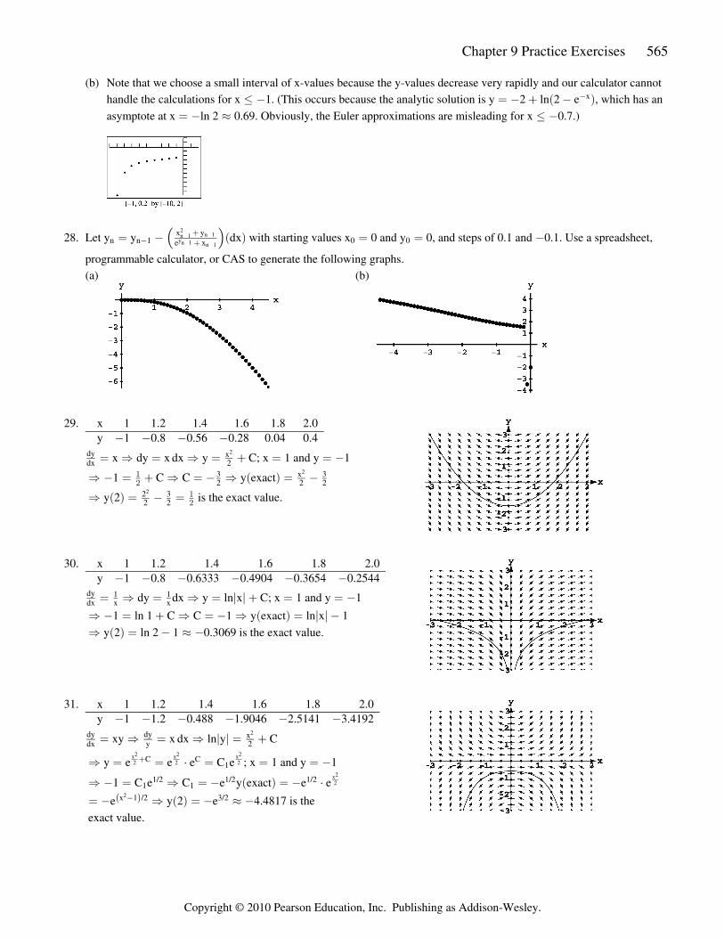
28. Let y y dx with starting values x 0 and y 0, and steps of 0.1 and 0.1. Use a spreadsheet,n n 1 0 0x ye xœ � œ œ ��

��Š ‹a b2

n 1 n 1yn 1 n 1

� �

��

programmable calculator, or CAS to generate the following graphs. (a) (b)

29. x 1 1.2 1.4 1.6 1.8 2.0y 1 0.8 0.56 0.28 0.04 0.4� � � �

x dy x dx y C; x 1 and y 1dydx 2

xœ Ê œ Ê œ � œ œ �2

1 C C y exactÊ � œ � Ê œ � Ê œ �"#

3 x 32 2 2a b 2

y 2 is the exact value.Ê œ � œa b 2 32 2

2 "#

30. x 1 1.2 1.4 1.6 1.8 2.0y 1 0.8 0.6333 0.4904 0.3654 0.2544� � � � � �

dy dx y ln x C; x 1 and y 1dydx x x

1 1œ Ê œ Ê œ � œ œ �k k 1 ln 1 C C 1 y exact ln x 1Ê � œ � Ê œ � Ê œ �a b k k y 2 ln 2 1 0.3069 is the exact value.Ê œ � ¸ �a b

31. x 1 1.2 1.4 1.6 1.8 2.0y 1 1.2 0.488 1.9046 2.5141 3.4192� � � � � �

xy x dx ln y Cdy dydx y 2

xœ Ê œ Ê œ �k k 2

y e e e C e ; x 1 and y 1Ê œ œ † œ œ œ �x x x2 2 2

2 2 2�C C1

1 C e C e y exact e eÊ � œ Ê œ � œ � †1 11/2 1/2 1/2a b x2

2

e y 2 e 4.4817 is theœ � Ê œ � ¸ �ˆ ‰x 1 /2 3/22� a b exact value.



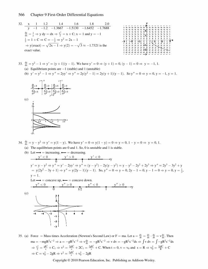
32. x 1 1.2 1.4 1.6 1.8 2.0y 1 1.2 1.3667 1.5130 1.6452 1.7688� � � � � �

y dy dx x C; x 1 and y 1dy ydx y 2

1œ Ê œ Ê œ � œ œ �2

1 C C y 2x 1" "# #œ � Ê œ � Ê œ �2

y exact 2x 1 y 2 3 1.7321 is theÊ œ � Ê œ � ¸ �a b a bÈ È exact value.

33. y 1 y y 1 y 1 . We have y 0 y 1 0, y 1 0 y 1, 1.dydx

2œ � Ê œ � � œ Ê � œ � œ Ê œ �w wa ba b a b a b (a) Equilibrium points are 1 (stable) and 1 (unstable)�

(b) y y 1 y 2yy y 2y y 1 2y y 1 y 1 . So y 0 y 0, y 1, y 1.w ww w ww wwœ � Ê œ Ê œ � œ � � œ Ê œ œ � œ2 2a b a ba b

(c)

34. y y y y 1 y . We have y 0 y 1 y 0 y 0, 1 y 0 y 0, 1.dydx

2œ � Ê œ � œ Ê � œ Ê œ � œ Ê œw wa b a b (a) The equilibrium points are 0 and 1. So, 0 is unstable and 1 is stable. (b) Let increasing, decreasing.ïî œ íï œ

yy y y

0 1qqíïïïïïqqñqqïïïïïîqqñqqíïïïïïqqp

� ! � ! � ! w w w

y y y y y 2yy y y y 2y y y y y 2y 2y y 2y 3y yw ww w w ww wwœ � Ê œ � Ê œ � � � œ � � � Ê œ � �2 2 2 2 2 3 3 2a b a b y 2y 3y 1 y y 2y 1 y 1 . So, y 0 y 0, 2y 1 0, y 1 0 y 0, y ,œ � � Ê œ � � œ Ê œ � œ � œ Ê œ œa b a ba b2 ww ww "

#

y 1.œ

Let concave up, concave down.ïî œ íï œ

yy y y y

0 11/2qíïïïïïqqñqqïïïïïîqqñqqíïïïïïqqñqqïïïïïîqp

� ! � ! � ! � !ww ww ww ww

(c)

35. (a) Force Mass times Acceleration (Newton's Second Law) or F ma. Let a v . Thenœ œ œ œ † œdv dv ds dvdt ds dt ds

ma mgR s a gR s v gR s v dv gR s ds v dv gR s dsœ � Ê œ � Ê œ � Ê œ � Ê œ �2 2 2 2 2 2 2 2 2 2dvds

� � � � �' ' C v 2C C. When t 0, v v and s R v CÊ œ � Ê œ � œ � œ œ œ Ê œ �v

2 s s s RgR 2gR 2gR 2gR

1 1 02 2

02 2 2 2 2

C v 2gR v v 2gRÊ œ � Ê œ � �2 2 20 0

2gRs

2


Chapter 9 Additional and Advanced Exercises 567

(b) If v 2gR, then v v , since v 0 if v 2gR. Then s ds 2gR dt0 02 2gR 2gR

s s dtds 2gR

s2œ œ Ê œ œ Ê œÈ ÈÉ È È2 2 2È

È

s ds 2gR dt s 2gR t C s 2gR t C; t 0 and s RÊ œ Ê œ � Ê œ � œ œ' '1/2 3/2 3/22 2 22 33 21È È Èˆ ‰

R 2gR 0 C C R s 2gR t R R 2g t RÊ œ � Ê œ Ê œ � œ �3/2 3/2 3/2 3/2 3/23 3 32 2 2

2 2ˆ ‰ ˆ ‰ ˆ ‰È Èa b È R R t 1 R s RR 2g t 1 t 1 1 tœ œ � œ Ê œ� � �3/2 3/2 3/23

21/2 3 2gR

2R3v 3v2R 2R

2/3� ‘ � ‘ � ‘ˆ ‰È ’ “Š ‹ ˆ ‰ ˆ ‰� È0 0

36. coasting distance 0.97 k 27.343. s t 1 e s t 0.97 1 ev m v mk k k

0.86 30.84 k/m t 27.343/30.84 t0 0œ Ê œ Ê ¸ œ � Ê œ �a ba b a b a ba b a bˆ ‰ ˆ ‰� �

s t 0.97 1 e . A graph of the model is shown superimposed on a graph of the data.Ê œ �a b a b�0.8866t

CHAPTER 9 ADDITIONAL AND ADVANCED EXERCISES

1. (a) k c y dy k y c dt k dt k dt ln y c k t Cdy dy dydt V V y c V y c V V

A A A A A1œ � Ê œ � � Ê œ � Ê œ � Ê � œ � �a b a b k k� �

' ' y c e e . Apply the initial condition, y 0 y y c C C y cÊ � œ „ œ Ê œ � Ê œ �C k t

0 0 01

AV� a b

y c y c e .Ê œ � �a b0k t� A

V

(b) Steady state solution: y y t c y c 0 cc y c e_Ä_ Ä_

�œ œ œ � � œ� �lim limt t 0

k t0a b a ba b� ‘a b A

V

2. F v u F v u F m v v u F m u .d mv d mvdt dt dt dt dt dt dt dt dt dt

dm dm dv dm dm dm dv dma b a bœ � � Ê œ � � Ê œ � � � Ê œ �a b a b b m b t C. At t 0, m m , so C m and m m b t.dm

dt 0 0 0œ � Ê œ � � œ œ œ œ �k k k k Thus, F m b t u b m b t g g v gt u ln Cœ � � œ � � Ê œ � � Ê œ � � �a b k k a bk kk k k k Š ‹0 0 1

dv dvdt dt m b t m

u b m b tk k k kk k0 0

0

��

v 0 at t 0 C 0. So v gt u ln y dt and u c, y 0 atgt u lnœ œ Ê œ œ � � œ Ê œ œ œ� �1m b t

m dtdy m b t

mŠ ‹ Š ‹0

0

0

0

� �k k k k' ’ “ t 0 y gt c t lnœ Ê œ � � �"

#

� �2 m b t m b tb m’ “Š ‹ Š ‹0 0

0

k k k kk k

3. (a) Let y be any function such that v x y v x Q x dx C, v x e . Thena b a b a b a bœ � œ' ' P x dxa b

v x y v x y y v x v x Q x . We have v x e v x e P x v x P x .ddx

P x dx P x dxa b a b a b a b a b a b a b a b a b a ba b † œ † � † œ œ Ê œ œ œw w w' 'a b a b

Thus v x y y v x P x v x Q x y y P x Q x the given y is a solution.a b a b a b a b a b a b a b† � † œ Ê � œ Êw w

(b) If v and Q are continuous on and x a, b , then v t Q t dt v x Q xa, bc d a b a b a b a b a b’ “− œddx x

x'0

v t Q t dt v x Q x dx. So C y v x v x Q x dx. From part (a), v x y v x Q x dx C.Ê œ œ � œ �'x

x0 0

0

a b a b a b a b a b a b a b a b a b a b' ' ' Substituting for C: v x y v x Q x dx y v x v x Q x dx v x y y v x when x x .a b a b a b a b a b a b a b a bœ � � Ê œ œ' '0 0 0 0 0

4. (a) y P x y 0, y x 0. Use v x e as an integrating factor. Then v x y 0 v x y Cw � œ œ œ œ Ê œa b a b a b a b a ba b0P x dx d

dx' a b

y Ce and y C e , y C e , y x y x 0, y y C C eÊ œ œ œ œ œ � œ �� #

' ' ' 'P x dx P x dx P x dx P x dx1 1 2 1 0 2 0 1 2 1 2

a b a b a b a ba b a b a b C e and y y 0 0 0. So y y is a solution to y P x y 0 with y x 0.œ � œ � œ � � œ œ3 1 2 1 2 0

P x dx� w' a b a b a b (b) v x e C C C .y x y x e C Cd d d d

dx dx dx dx1 2P x dx P x dx

1 2 1 2 3a b a b a ba bc da b a b Š ‹� ‘a b� œ œ � œ œ !�' 'a b a b�

v x dx v x dx Cy x y x y x y x' 'ddx 1 2 1 2a b a ba bc d a bc da b a b a b a b� �œ œ ! œ



(c) y C e , y C e , y y y . So y x 0 C e C e1 1 2 1 2 0 1P x dx P x dx P x dx P x dxœ œ œ � œ Ê � œ !� � � �

# #' ' ' 'a b a b a b a ba b

C C 0 C C y x y x for a x b.Ê � œ Ê œ Ê œ � �1 2 1 2 1 2a b a b

5. x y dx x y dy 0 F F v v 0a b a bˆ ‰2 2 dy y y ydx x y y x y x x x v x v F v

x y x 1 1 dx dv� � œ Ê œ œ � � œ � � œ Ê œ � � Ê � œ� �

Î �

ˆ ‰a b

2 2

0 C ln x ln 2v 1 C 4ln x ln 2 1 CÊ � œ Ê � œ Ê l l � l � l œ Ê l l � l � l œdx dv dx v dv 1x x 2v 1 4 xv v

2 y 2

� � � �ˆ ‰1 2v

' ' ˆ ‰ ln x ln C ln x 2y x C x 2y x e x 2y x CÊ l l � œ Ê � œ Ê � œ Ê � œ4 2 2 2 2 2 2 C 2 2 22y x

xº º ¹ ¹a b a b a b2 2

2�

6. x dy y x y dx 0 F F v v v 02 2 2dy dy y y ydx x dx x x x x v v v

y x y 2 dx dv� � œ Ê œ Ê œ � � œ Ê œ � � Ê � œa b a bˆ ‰ ˆ ‰� �

� � �

ˆ ‰a b

2

2 2

C ln x C ln x C ln x CÊ � œ Ê l l � œ Ê l l � œ Ê l l � œ' 'dx dv 1 1 xx v v y x y2 Î

7. x e y dx x dy 0 e F F v e v 0ˆ ‰ ˆ ‰ a by x y x vdy x e y y ydx x x x x v e v

dx dvÎ Î�� œ Ê œ œ � œ Ê œ � Ê � œ

y x

v

Î

a b

C ln x e C ln x e CÊ � œ Ê l l � œ Ê l l � œ' 'dx dvx e

v y xv

� � Î

8. x y dy x y dx 0 F F v 0a b a b a bˆ ‰� � � œ Ê œ œ œ Ê œ Ê � œdy ydx x y x 1 v x

x y 11

v 1 dx dvv

� ��

�

��

�

a bˆ ‰

yx

yx

v 11 v�

�

0 0 ln x tan v ln v 1 CÊ � œ Ê � � œ Ê l l � � l � l œ' ' ' ' 'dx dx dv v dv 1x v 1 x v 1 v 1 2

1 v dv 1 2a b��

�2 2 2

2 ln x 2 tan v ln 1 C ln x 2 tan ln C 2 tan ln y x CÊ l l � � � œ Ê l l � � œ Ê � � œ� � ��1 2 1 1 2 2y y y x yx x x x

2¹ ¹ ¹ ¹ˆ ‰ ˆ ‰ ˆ ‰º º2 2

2

9. y cos cos 1 F F v v cos v 1 0w �� œ � œ � � œ Ê œ � � Ê � œy y x y y y

x x x x x x v v cos v 1dx dvˆ ‰ ˆ ‰ ˆ ‰ a b a b a ba b

sec v 1 dv 0 ln x ln sec v 1 tan v 1 C ln x ln sec 1 tan 1 CÊ � � œ Ê l l � l � � � l œ Ê l l � � � � œ' 'dxx x x

y ya b a b a b ¹ ¹ˆ ‰ ˆ ‰

10. x sin y cos dx x cos dy 0 tan F F v v tan vˆ ‰ ˆ ‰ a by y y dy y y yx x x dx x x x

x sin y cosx cos� � œ Ê œ œ � œ Ê œ �

� �ˆ ‰y yx x

yx

0 cot v dv 0 ln x ln sin v C ln x ln sin CÊ � œ Ê � œ Ê l l � l l œ Ê l l � œdx dv dxx v v tan v x x

y� �a b

' ' ¹ ¹


section 9.4 graphical solutions of autonomous equations 553

Documents