Section 3

VOC Controls

EPA/452/B-02-001

Section 3.1

VOC Recapture Controls

EPA/452/B-02-001

1-1

Chapter 1

Carbon Adsorbers

William M. Vatavuk

Innovative Strategies and Economics Group, OAQPS

U.S. Environmental Protection Agency

Research Triangle Park, NC 27711

William L. Klotz

Chas. T. Main, Inc.

Charlotte, NC 28224

Robert L. Stallings

Ozone Policy and Strategies Group, OZQPS

U.S. Environmental Protection Agency

Research Triangle Park, NC 27711

September 1999

EPA/452/B-02-001

1-2

Contents

1.0 Introduction ............................................................................................................................... 1-3

1.1 Types of Adsorbers ................................................................................................................... 1-3

1.1.1 Fixed-bed Units ................................................................................................................ 1-3

1.1.2 Cannister Units ................................................................................................................. 1-5

1.1.3 Adsorption Theory .......................................................................................................... 1-6

1.2 Design Procedure ...................................................................................................................... 1-12

1.2.1 Sizing Parameters ............................................................................................................. 1-12

1.2.2 Determining Adsorption and Desorption Times .............................................................. 1-13

1.2.3 Estimating Carbon Requirement ....................................................................................... 1-15

1.2.3.1 Overview of Carbon Estimation Procedures ....................................................... 1-15

1.2.3.2 Carbon Estimation Procedure Used in Manual ................................................... 1-15

1.3 Estimating Total Capital Investment .......................................................................................... 1-17

1.3.1 Fixed-Bed Systems ........................................................................................................... 1-17

1.3.1.1 Carbon Cost ........................................................................................................ 1-17

1.3.1.2 Vessel Cost ......................................................................................................... 1-18

1.3.1.3 Total Purchased Cost .......................................................................................... 1-21

1.3.1.4 Total Capital Investment ..................................................................................... 1-23

1.3.2 Cannister Systems ............................................................................................................ 1-23

1.4 Estimating Total Annual Cost ................................................................................................... 1-24

1.4.1 Direct Annual Costs ......................................................................................................... 1-24

1.4.1.1 Steam1-281-25

1.4.1.2 Cooling Water ..................................................................................................... 1-25

1.4.1.3 Electricity ........................................................................................................... 1-26

1.4.1.4 Carbon Replacement ........................................................................................... 1-29

1.4.1.5 Solid Waste Disposal .......................................................................................... 1-29

1.4.1.6 Operating and Supervisory Labor ...................................................................... 1-30

1.4.1.7 Maintenance Labor and Materials ...................................................................... 1-30

1.4.2 Indirect Annual Costs ...................................................................................................... 1-30

1.4.3 Recovery Credits .............................................................................................................. 1-31

1.4.4 Total Annual Cost ............................................................................................................ 1-32

1.4.5 Example Problem............................................................................................................... 1-32

1-3

1.0 Introduction

In air pollution control, adsorption is employed to remove volatile organic compounds

(VOCs) from low to medium concentration gas streams, when a stringent outlet concentration

must be met and/or recovery of the VOC is desired. Adsorption itself is a phenomenon where gas

molecules passing through a bed of solid particles are selectively held there by attractive forces

which are weaker and less specific than those of chemical bonds. During adsorption, a gas molecule

migrates from the gas stream to the surface of the solid where it is held by physical attraction

releasing energy—the “heat of adsorption”, which typically equals or exceeds the heat of

condensation. Adsorptive capacity of the solid for the gas tends to increase with the gas phase

concentration, molecular weight, diffusivity, polarity, and boiling point. Gases form actual chemical

bonds with the adsorbent surface groups. This phenomenon is termed “chemisorption”.

Most gases (“adsorbates”) can be removed (“desorbed”) from the adsorbent by heating

to a sufficiently high temperature, usually via steam or (increasingly) hot combustion gases, or by

reducing the pressure to a sufficiently low value (vacuum desorption). The physically adsorbed

species in the smallest pores of the solid and the chemisorbed species may require rather high

temperatures to be removed, and for all practical purposes cannot be desorbed during regeneration.

For example, approximately 3 to 5 percent of organics adsorbed on virgin activated carbon is

either chemisorbed or very strongly physically adsorbed and is difficult to desorb during

regeneration.[1]

Adsorbents in large scale use include activated carbon, silica gel, activated alumina, synthetic

zeolites, fuller’s earth, and other clays. This section is oriented toward the use of activated carbon,

a commonly used adsorbent for VOCs.

1.1 Types of Adsorbers

Five types of adsorption equipment are used in collecting gases: (1) fixed regenerable

beds; (2) disposable/rechargeable cannisters; (3) traveling bed adsorbers; (4) fluid bed adsorbers;

and (5) chromatographic baghouses.[2] Of these, the most commonly used in air pollution control

are fixed-bed systems and cannister types. This section addresses only fixed-bed and cannister

units.

1.1.1 Fixed-bed Units

Fixed-bed units can be sized for controlling continuous, VOC-containing streams over a

wide range of flow rates, ranging from several hundred to several hundred thousand cubic feet per

minute (cfm). The VOC concentration of streams that can be treated by fixed-bed adsorbers can

be as low as several parts per billion by volume (ppbv) in the case of some toxic chemicals or as

1-4

high as 25% of the VOCs’ lower explosive limit (LEL). (For most VOCs, the LEL ranges from

2500 to 10,000 ppmv.[3])

Fixed-bed adsorbers may be operated in either intermittent or continuous modes. In

intermittent operation, the adsorber removes VOC for a specified time (the “adsorption time”),

which corresponds to the time during which the controlled source is emitting VOC. After the

adsorber and the source are shut down (e.g., overnight), the unit begins the desorption cycle

during which the captured VOC is removed from the carbon. This cycle, in turn, consists of three

steps: (1) regeneration of the carbon by heating, generally by blowing steam through the bed in the

direction opposite to the gas flow;1(2) drying of the bed, with compressed air or a fan; and (3)

cooling the bed to its operating temperature via a fan. (In most designs, the same fan can be used

both for bed drying and cooling.) At the end of the desorption cycle (which usually lasts 1 to 1½

hours), the unit sits idle until the source starts up again.

In continuous operation a regenerated carbon bed is always available for adsorption, so

that the controlled source can operate continuously without shut down. For example, two carbon

beds can be provided: while one is adsorbing, the second is desorbing/idled. As each bed must be

large enough to handle the entire gas flow while adsorbing, twice as much carbon must be provided

than an intermittent system handling the same flow. If the desorption cycle is significantly shorter

than the adsorption cycle, it may be more economical to have three, four, or even more beds

operating in the system. This can reduce the amount of extra carbon capacity needed or provide

some additional benefits, relative to maintaining a low VOC content in the effluent. (See Section

1.2 for a more thorough discussion of this.)

A typical two-bed, continuously operated adsorber system is shown in Figure 3.1. One

of the two beds is adsorbing at all times, while the other is desorbing/idled. As shown here, the

VOC-laden gas enters vessel #1 through valve A, passes through the carbon bed (shown by the

shading) and exits through valve B, from whence it passes to the stack. Meanwhile, vessel #2 is in

the desorption cycle. Steam enters through valve C, flows through the bed and exits through D.

The steam-VOC vapor mixture passes to a condenser, where cooling water condenses the entire

mixture. If part of the VOC is immiscible in water, the condensate next passes to a decanter,

where the VOC and water layers are separated. The VOC layer is conveyed to storage. If

impure, it may receive additional purification by distillation. Depending on its quality (i.e., quantity

of dissolved organics), the water layer is usually discharged to a wastewater treatment facility.

1

Although steam is the most commonly used regenerant, there are situations where it should not be used

An example would be a degreasing operation that emits halogenated VOCs. Steaming might cause the

VOCs to decompose.

1-5

1.1.2 Cannister Units

Cannister-type adsorbers originally refered to relatively small returnable containers, such

as 55-gallon drums. Cannisters differ from fixed-bed units, in that they are normally limited to

controlling lower-volume and intermittent gas streams, such as those emitted by storage tank

vents, where process economics dictate that off-site regeneration is appropriate. The carbon

cannisters are not intended for desorption on-site. However, the carbon may be regenerated at a

central facility. The term cannister is becoming something of a misnomer as much of the growth in

the industry is in larger vessels without regeneration capabilities. Calgon provided information on

standard systems as large as 8,000 cfm and carbon capacitites of 2,000 pounds; TIGG Corporation

reported systems as large as 30,000 cfm. [4][5]

Figure 1.1: Typical-Two-Bed, Continuously Operated Fixed

Bed Carbon Adsorber System

Decanter,distillation

column

Duct

Purified airexhaust

Vapor-airmixture

Blower

Adsorber

Particulatefilter

Condenser

Recoveredsolvent

Steamgenerator

Hoods or direct connections to point-emission sources

Bed 1

Carbon Bed

on-stream

Bed 2

Carbon Bed

regenerating

1-6

Once the carbon reaches a certain VOC content, the unit is shut down and either the

carbon or the cannister is replaced. The carbon or cannister is then returned to a reclaimation

facility or regenerated at the central facility. Each cannister unit consists of a vessel, activated

carbon, inlet connection and distributer leading to the carbon bed, and an outlet connection for the

purified gas stream. In one design (Calgon’s Ventsorb® ), 180 lbs of carbon are installed on an 8-

inch gravel bed, in a 55-gallon drum with an internal collector. The type of carbon used depends

on the nature of the VOC to be treated [6]. Non-regenrable vessles can be placed in a series, this

protects agianst breakthrough because in the event that the first cannister or vessel becomes saturated

with VOC, the second then becomes the primary carbon adsorber. One option would be to

periodically remove the most saturated cannister or carbon bed and add a fresh cannister or

carbon bed to the clean end. Periodic sampling for breakthrough between the carbon beds would

assure that replacement occured frequently enough to avoid breakthrough to the atmosphere. This

approach also improves cost effectiveness of carbon replacement because the carbon is at or near

its saturation point when it is replaced.

In theory, a cannister unit would remain in service longer than a regenerable unit would

stay in its adsorption cycle due to a higher theoretical capacity for fresh carbon compared to

carbon regenrated on-site. The service life is based on a service factor determined by the ratio of

the theoretical capacity to the working capacity. Determining service factors help to insure the

allowable outlet concentration from being exceeded. In reality, however, poor operating practice

may result in the cannister remaining connected until the carbon is near or at saturation. This is

because: (1) the carbon (and often the vessel) will probably be disposed of, so there is the temptation

to operate it until the carbon is saturated; and (2) unlike fixed-bed units, whose outlet VOC

concentrations are usually not monitored continuously (via flame ionization detectors, typically),

canisters are usually not monitored. Adequate recordeeping and periodic monitoring for

breakthrough can be supported by bed life modeling provided by vendors to ensure that cannister

replacement occurs with sufficient frequency and that breakthrough does not occur.

1.1.3 Adsorption Theory

At equilibrium, the quantity of gas that is adsorbed on activated carbon is a function of the

adsorption temperature and pressure, the chemical species being adsorbed, and the carbon

characteristics, such as carbon particle size and pore structure. For a given adsorbent-VOC

combination at a given temperature, an adsorption isotherm can be constructed which relates the

mass of adsorbate per unit weight of adsorbent (“equilibrium adsorptivity”) to the partial pressure

of the VOC in the gas stream. The adsorptivity increases with increasing VOC partial pressure

and decreases with increasing temperature.

A family of adsorption isotherms having the shape typical of adsorption on activated carbon

is plotted in Figure 3.2. This and other isotherms whose shapes are convex upward throughout,

1-7

are designated “Type I” isotherms. The Freundlich isotherm, which can be fit to a portion of a

Type I curve, is commonly used in industrial design.[2]

W = k Pe m

(1.1)

where

we

= equilibrium adsorptivity (lb adsorbate/lb adsorbent)

P = partial pressure of VOC in gas stream (psia)

k,m = empirical parameters

The treatment of adsorption from gas mixtures is complex and beyond the scope of this chapter.

Except where the VOC in these mixtures have nearly identical adsorption isotherms, one VOC in

a mixture will tend to displace another on the carbon surface. Generally, VOCs with lower vapor

pressures will displace those with higher vapor pressure, resulting in the former displacing the latter

previously adsorbed. Thus, during the course of the adsorption cycle the carbon’s capacity for a

higher vapor pressure constituent decreases. This phenomenon should be considered when sizing

the adsorber. To be conservative, one would normally base the adsorption cycle requirements on

the least adsorbable component in a mixture and the desorption cycle on the most adsorbable

component.[1]

The equilibrium adsorptivity is the maximum amount of adsorbate the carbon can hold at a

given temperature and VOC partial pressure. In actual control systems where there are not two

beds operating in series, however, the entire carbon bed is never allowed to reach equilibrium.

Instead, once the outlet concentration reaches a preset limit (the “breakthrough concentration”),

the adsorber is shut down for desorption or (in the case of cannister units) replacement and disposal.

At the point where the vessel is shut down, the average bed VOC concentration may only be 50%

or less of the equilibrium concentration. That is, the carbon bed may be at equilibrium (“saturated”)

at the gas inlet, but contain only a small quantity of VOC near the outlet.

As Equation 3.1 indicates, the Freundlich isotherm is a power function that plots as a

straight line on log-log paper. Conveniently, for the concentrations/partial pressures normally

encountered in carbon adsorber operation, most VOC-activated carbon adsorption conforms to

Equation 3.1. At very low concentrations, typical of breakthrough concentrations, a linear

approximation (on arithmetic coordinates) to the Freundlich isotherm is adequate. However, the

Freundlich isotherm does not accurately represent the isotherm at high gas concentrations and thus

should be used with care as such concentrations are approached.

Adsorptivity data for selected VOCs were obtained from Calgon Corporation, a vendor

of activated carbon.[6] The vendor presents adsorptivity data in two forms: a set of graphs displaying

equilibrium isotherms [6] and as a modification of the Dubinin-Radushkevich (D-R) equation, a

semi-empirical equation that predicts the adsorptivity of a compound based on its adsorption

1-8

potential and polarizability.[8] In this Manual, the modified D-R equation is referred to as the

Calgon fifth-order polynomial. The data displayed in the Calgon graphs [6] has been fit to the

Freundlich equation. The resulting Freundlich parameters are shown in Table 1.1 for a limited

number of chemicals. The adsorbates listed include aromatics (e.g., benzene, toluene), chlorinated

aliphatics (dichloroethane), and one ketone (acetone). However, the list is far from all-inclusive.

Notice that a range of partial pressures is listed with each set of parameters, k and m.

(Note: In one case (m-xylene) the isotherm was so curvilinear that it had to be split into two parts,

each with a different set of parameters.) This is the range to which the parameters apply.

Extrapolation beyond this range—especially at the high end—can introduce inaccuracy to the

calculated adsorptivity.

But high-end extrapolation may not be necessary, as the following will show. In most air

pollution control applications, the system pressure is approximately one atmosphere (14.696 psia).

The upper end of the partial pressure ranges in Table 1.1 goes from 0.04 to 0.05 psia. According

to Dalton’s Law, at a total system pressure of one atmosphere this corresponds to an adsorbate

concentration in the waste gas of 2,720 to 3,400 ppmv. Now, as discussed in Section 1.1.2, the

adsorbate concentration is usually kept at 25% of the lower explosive limit (LEL).2 For many

VOCs, the LEL ranges from 1 to 1.5 volume %, so that 25% of the LEL would be 0.25 to

2

Although, Factory Mutual Insurance will reportedly permit operation at up to 50% of the LEL, if proper

VOC monitoring is used.

Adsorbate Partial Pressure (psia)

(Note: T1<T2<T3<T4)

T4

T3

T2

T1

Equ

ilibr

ium

Ads

orpt

ivity

(lb

ads

orba

te/lb

ads

orbe

nt)

( F)

Figure 1.2: Type I Adsorption Isotherms for Hypothetical Adsorbate

1-9

0.375% or 2,500 to 3,750 ppmv, which approximates the high end of the partial pressure ranges

in Table 1.1.

Finally, each set of parameters applies to a fixed adsorption temperature, ranging from 77o

to 104o F. These temperatures reflect typical operting conditions, although adsorption can take

Table 1.1: Parameters for Selected Adsorption Isotherms [6]a

Adsorbate Adsorption Isotherm Range of Isothermb

Temp (oF) Parameters (psia) k m

Benzene 77 0.597 0.176 0.0001-0.05

Chlorobenzene 77 1.05 0.188 0.0001-0.01

Cyclohexane 100 0.505 0.210 0.0001-0.05

Dichloroethane 77 0.976 0.281 0.0001-0.04

Phenol 104 0.855 0.153 0.0001-0.03

Trichloroethane 77 1.06 0.161 0.0001-0.04

Vinyl Chloride 100 0.200 0.477 0.0001-0.05

m-Xylene 77 0.708 0.113 0.0001-0.001

77 0.527 0.0703 0.001-0.05

Acrylonitrile 100 0.935 0.424 0.0001-0.015

Acetone 100 0.412 0.389 0.0001-0.05

Toluene 77 0.551 0.110 0.001-0.05

a Each isotherm is of the for We=kPp. (See text for definition of terms.) Data are for adsorption of Calgon type “BPL”

carbon.b Equation should not be extrapolated outside these ranges.

The Calgon fifth-order polynomial is somewhat more accurate than the Freundilich parameters

from Table 1.1. The polynomial contains a temperature parameter, and it allows one to estimate

adsorption isotherms for compounds not shown in Table 1.1 if pure component data are available.

The pure component data required are the saturation pressure, liquid molar volume, and the refractive

index. It is, however, somewhat more complex to use than the Freundlich equation. The Calgon

fifth-oder polynomial is as follows:

The mass loading, we, is calculated from

w . G

VMW

e

m

ads=

0 01

(1.2)

1-10

3

This, of course, is equal to lb absorbate per lb carbon.

place as low as 32oF and even higher than 104oF. As the adsorption temperature increases to

much higher levels, however, the equilibrium adsorptivity decreases to such an extent that VOC

recovery by carbon adsorption may become economically impractical.

where

we

= mass loading, i.e., equilibrium adsorptivity (g adsorbate per g carbon)3

G = carbon loading at equilibrium (cm3 liquid adsorbate per 100 g carbon)

Vm

= liquid molar volume of adsorbate (cm3 per g-mole).

MWads

= molecular weight of Adsorbute

Note that the terms in Equation 1.2 are given in metric units, not English. This has been

done because the carbon loading, G, is calculated from a regression equation in which all the terms

are expressed in metric units. This equation for G is the Calgon fifth-order polynomial:

log (G) A A Y A Y A Y A Y A Y10 0 1 2

2

3

3

4

4

5

5 = + + + + + (1.3)

where

A0

= 1.71

Al

= -1.46 × 10-2

A2

= -1.65 × 10-3

A3

= -4.11 × 10-4

A4

= +3.14 x 10-5

A5

= -6.75 x 10-7

and Y is calculated from several equations which follow.

The first step in calculating Y is to calculate P. This can be done by calculating the adsorption

potential, ε :

ε = RT lnP

P

s

i

(1.4)

where

R = 1.987 (calories per g-mole- K

T = absolute temperature ( K)

Ps

= vapor pressure of adsorbate at the temperature T (kPa)

Pi

= partial pressure of adsorbate (kPa).

1-11

The χ is calculated from:

( )χε

= 2 303. R V

m

(1.5)

By substituting for , in the above equation, P can alternatively be calculated from4:

χ =

T

Vlog

P

Pm

s

i

10 (1.6)

The next step in calculating Y is to calculate the relative polarizability, '.

ΓΘΘ

= i

o

(1.7)

where

1i

= polarizability of component i per unit volume, where component i is the

adsorbate

1o

= polarizability of component o per unit volume, where component o is

the reference component, n-heptane.

For the adsorbate or the reference compound, using the appropriate refractive index of adsorbate,

n, the polarizability is calculated from:

Θ = n -

n +

2

2

1

2(1.8)

Once P and ' are known, Y can be calculated from:

Y = χΓ

(1.9)

Calgon also has a proprietary, seventh-order form in which two additional coefficients are

added to the Calgon fifth-order polynomial, but the degree of fit reportedly is improved only

modestly.[8] Additional sources of isotherm data include the activated carbon vendors, handbooks

(such as Perry’s Chemical Engineer’s Handbook), and the literature.

4 Alternatively, if the available values for T, Pi, P

s, and Vm are in English units, they may be substitued into this equation without

conversion. However, to make the result dimensionally consistent with Equation 1.3, it would have to be multiplied by a

conversion factor, 34.7.

1-12

1.2 Design Procedure

1.2.1 Sizing Parameters

Data received from adsorber vendors indicate that the size and purchase cost of a fixed-

bed or cannister carbon adsorber system primarily depend on five parameters:

1. The volumetric flow of the VOC laden gas passing through the carbon bed(s);

2. The inlet and outlet VOC mass loadings of the gas stream;

3. The adsorption time (i.e,. the time a carbon bed remains on-line to adsorb VOC

before being taken off-line for desorption of the bed);

4. The working capacity of the activated carbon in regenerative systems or the equilibrium

cpacity in the case of non-regenerative systems,

5. The humidity of the gas stream, especially in the effect of humidy on capacity in relation to

halogens.

In addition, the cost could also be affected by other stream conditions, such as the presence/

absence of excessive amounts of particulate, moisture, or other substances which would require

the use of extensive pretreatment and/or corrosive-resistant construction materials.

The purchased cost depends to a large extent on the volumetric flow (usually measured in

actual ft3/min). The flow, in turn, determines the size of the vessels housing the carbon, the capacities

of the fan and motor needed to convey the waste gas through the system, and the diameter of the

ducting.

Also important are the VOC inlet and outlet gas stream loadings, the adsorption time, and

the working or equilibium capacity of the carbon. These variables determine the amount and cost

of carbon charged to the system initially and, in turn, the cost of replacing that carbon after it is

exhausted (typically, five years after startup). Moreover, the amount of the carbon charge affects

the size and cost of the auxiliary equipment (condenser, decanter, bed drying/cooling fan), because

the sizes of these items are tied to the amount of VOC removed by the bed. The amount of carbon

also has a bearing on the size and cost of the vessels.

A carbon adsorber vendor [9] supplied data that illustrate the dependency of the equipment

cost on the amount of the carbon charge. Costs were obtained for fixed-bed adsorbers sized to

handle three gas flow rates ranging from 4,000 to 100,000 scfm and to treat inlet VOC (toluene)

concentrations of 500 and 5,000 ppm. Each adsorber was assumed to have an eight-hour

1-13

adsorption time. As one might expect, the equipment costs for units handling higher gas flow rates

were higher than those handling lower gas flow rates. Likewise, at each of the gas flow rates, the

units sized to treat the 5,000 ppm VOC streams had higher equipment costs than those sized to

treat the 500 ppm concentration. These cost differences ranged from 23 to 29% and averaged

27%. These higher costs were partly needed to pay for the additional carbon required to treat the

higher concentration streams. But some of these higher costs were also needed for enlarging the

adsorber vessels to accommodate the additional carbon and for the added structural steel to

support the larger vessels. Also, larger condensers, decanters, cooling water pumps, etc., were

necessary to treat the more concentrated streams. (See Section 1.3.)

The VOC inlet loading is set by the source parameters, while the outlet loading is set by

the VOC emission limit. (For example, in many states, the average VOC outlet concentration from

adsorbers may not exceed 25 ppm.)

1.2.2 Determining Adsorption and Desorption Times

The relative times for adsorption and desorption and the adsorber bed configuration (i.e.,

whether single or multiple and series or parallel adsorption beds are used) establish the adsorption/

desorption cycle profile. The circle profile is important in determining carbon and vessel requirements

and in establishing desorption auxiliary equipment and utility requirements. An example will illustrate.

In the simplest case, an adsorber would be controlling a process which emits a relatively small

amount of VOC intermittently—say, during one 8-hour shift per day. During the remaining 16

hours the system would either be desorbing or on standby. Properly sized, such a system would

only require a single bed, which would contain enough carbon to treat eight hours worth of gas

flow at the specified inlet concentration, temperature, and pressure. Multiple beds, operating in

parallel, would be needed to treat large gas flows (>100,000 actual ft3/min, generally)[9], as there

are practical limits to the sizes to which adsorber vessels can be built. But, regardless of whether

a single bed or multiple beds were used, the system would only be on-line for part of the day.

However, if the process were operating continuously (24 hours), an extra carbon bed

would have to be installed to provide adsorptive capacity during the time the first bed is being

regenerated. The amount of this extra capacity must depend on the number of carbon beds that

would be adsorbing at any one time, the length of the adsorption period relative to the desorption

period, and whether the beds were operating in parallel or in series. If one bed were adsorbing, a

second would be needed to come on-line when the first was shut down for desorption. In this

case, 100% extra capacity would be needed. Similarly, if five beds in parallel were operating in a

staggered adsorption cycle, only one extra bed would be needed and the extra capacity would be

20% (i.e., 1/5)—provided, of course, that the adsorption time were at least five times as long as

the desorption time. The relationship between adsorption time, desorption time, and the required

extra capacity can be generalized.

1-14

M = M fc c

I(1.10)

where

Mc,MccI

= amounts of carbon required for continuous or intermittent control of a

given source, respectively (lbs)

f = extra capacity factor (dimensionless)

This equation shows the relationship between Mc and M

CI. Section 1.2.3 shows how to calculate

these quantities.

The factor, f, is related to the number of beds adsorbing (NA) and desorbing (N

D) in a

continuous system as follows:

f N

N

D

A

= + 1 (1.11)

(Note: NA is also the number of beds in an intermittent system that would be adsorbing at any

given time. The total number of beds in the system would be NA + N

D.)

It can be shown that the number of desorbing beds required in a continuous system (ND)

is related to the desorption time ( θD), adsorption time ( θ

A), and the number of adsorbing beds,

as follows:

θ θD A

D

A

N

N ≤

(1.12)

(Note: 2D is the total time needed for bed regeneration, drying, and cooling.)

For instance, for an eight-hour adsorption time, in a continuously operated system of seven beds

(six adsorbing, one desorbing) 2Dwould have to be 1-1/3 hours or less (8 hours/6 beds). Otherwise,

additional beds would have to be added to provide sufficient extra capacity during desorption.

1-15

1.2.3 Estimating Carbon Requirement

1.2.3.1 Overview of Carbon Estimation Procedures

Obtaining the carbon requirement (Mc or M

cI) is not as straightforward as determining the

other adsorber design parameters. When estimating the carbon charge, the sophistication of the

approach used depends on the data and calculational tools available.

One approach for obtaining the carbon requirement is a rigorous one which considers the

unsteady-state energy and mass transfer phenomena occurring in the adsorbent bed. Such a

procedure necessarily involves a number of assumptions in formulating and solving the problem.

Such a procedure is beyond the scope of this Manual at the present time, although ongoing work

in the Agency is addressing this approach.

In preparing this section of the Manual, we have adopted a rule-of-thumb procedure for

estimating the carbon requirement. This procedure, while approximate in nature, appears to have

the acceptance of vendors and field personnel. It is sometimes employed by adsorber vendors to

make rough estimates of carbon requirement and is relatively simple and easy to use. It normally

yields results incorporating a safety margin, the size of which depends on the bed depth (short

beds would have less of a safety margin than deep beds), the effectiveness of regeneration, the

particular adsorbate and the presence or absence of impurities in the stream being treated.

1.2.3.2 Carbon Estimation Procedure Used in Manual

The rule-of-thumb carbon estimation procedure is based on the “working capacity” (We,

lb VOC/lb carbon). This is the difference per unit mass of carbon between the amount of VOC on

the carbon at the end of the adsorption cycle and the amount remaining on the carbon at the end of

the desorption cycle. It should not be confused with the “equilibrium capacity” (We,) defined

above in Section 1.1.3. Recall that the equilibrium capacity measures the capacity of virgin activated

carbon when the VOC has been in contact with it (at a constant temperature and partial pressure)

long enough to reach equilibrium. In adsorber design, it would not be feasible to allow the bed to

reach equilibrium. If it were, the outlet concentration would rapidly increase beyond the allowable

outlet (or “breakthrough”) concentration until the outlet concentration reached the inlet concentration.

During this period the adsorber would be violating the emission limit. With non-regenerable

(cannister) type systems, placing multiple vessles in a series can substantially decrease concerns of

breakthrough.

The working capacity is some fraction of the equilibrium capacity. Like the equilibrium

adsorptivity, the working capacity depends upon the temperature, the VOC partial pressure, and

the VOC composition. The working capacity also depends on the flow rate and the carbon bed

parameters.

1-16

The working capacity, along with the adsorption time and VOC inlet loading, is used to

compute the carbon requirement for a cannister adsorber or for an intermittently operated fixed-

bed adsorber as follows:

M = m

w

c

voc

e

AI

θ (1.13)

where

mvoc

= VOC inlet loading (lb/h)

Combining this with Equations 1.10 and 1.11 yields the general equation for estimating the system

total carbon charge for a continuously operated system:

M = m

w

N

Nc

voc

c

A

D

A

θ 1 +

(1.14)

Values for wc may be obtained from knowledge of operating units. If no value for w

c is available

for the VOC (or VOC mixture) in question, the working capacity may be estimated at 50% of the

equilibrium capacity, as follows:

w wc e(max)≈ 05. (1.15)

where

we(max)

= the equilibrium capacity (lb VOC/lb carbon) taken at the adsorber inlet (i.e., the

point of maximum VOC concentration).

(Note: To be conservative, this 50% figure should be lowered if short desorption cycles, very high

vapor pressure constituents, high moisture contents significant amounts of impurities, or difficult-

to-desorb VOCs are involved. Furthermore, the presence of strongly adsorbed impurities in the

inlet VOC stream may significantly shorten carbon life.)

As Equation 1.14 shows, the carbon requirement is directly proportional to the adsorption

time. This would tend to indicate that a system could be designed with a shorter adsorption time

to minimize the carbon requirement (and equipment cost). There is a trade-off here not readily

apparent from Equation 1.14, however. Certainly, a shorter adsorption time would require less

carbon. But, it would also mean that a carbon bed would have to be desorbed more frequently.

This would mean that the regeneration steam would have to be supplied to the bed(s) more frequently

to remove (in the long run) the same amount of VOC. Further, each time the bed is regenerated

1-17

the steam supplied must heat the vessel and carbon, as well as drive off the adsorbed VOC. And

the bed must be dried and cooled after each desorption, regardless of the amount of VOC removed.

Thus, if the bed is regenerated too frequently, the bed drying/cooling fan must operate more often,

increasing its power consumption. Also, more frequent regeneration tends to shorten the carbon

life. As a rule-of-thumb, the optimum regeneration frequency for fixed-bed adsorbers treating

streams with moderate to high VOC inlet loadings is once every 8 to 12 hours.[1]

1.3 Estimating Total Capital Investment

Entirely different procedures should be used to estimate the purchased costs of fixed-bed

and cannister-type adsorbers. Therefore, they will be discussed separately.

1.3.1 Fixed-Bed Systems

As indicated in the previous section, the purchased cost is a function of the volumetric flow

rate, VOC inlet and outlet loadings, the adsorption time, and the working capacity of the activated

carbon. As Figure 3.1 shows, the adsorber system is made up of several different items. Of these,

the adsorber vessels and the carbon comprise from one-half to nearly 90% of the total equipment

cost. (See Section 1.3.1.3.) There is also auxiliary equipment, such as fans, pumps, condensers,

decanters, and internal piping. But because these usually comprise a small part of the total purchased

cost, they may be “factored” from the costs of the carbon and vessels without introducing significant

error. The costs of these major items will be considered separately.

1.3.1.1 Carbon Cost

Cabon Cost, Cc, in dollars ($) is simply the product of the initial carbon requirement (M

c)

and the current price of carbon. As adsorber vendors buy carbon in very large quantities (million-

pound lots or larger), their cost is somewhat lower than the list price. For larger systems (other

than cannister) Calgon reports typical carbons costs to be $0.75 to $1.25 for virgin carbon and

$0.50 to $0.75 for reactiviated carbon (mid-1999 dollars). A typical of $1.00/lb is used in the

calculation below.[5][10] Thus:

C Mc c

= 100. (1.16)

1.3.1.2 Vessel Cost

The cost of an adsorber vessel is primarily determined by its dimensions which, in turn,

depend upon the amount of carbon it must hold and the superficial gas velocity through the bed

that must be maintained for optimum adsorption. The desired superficial velocity is used to calculate

the cross-sectional area of the bed perpendicular to the gas flow. An acceptable superficial velocity

is established empirically, considering desired removal efficiency, the carbon particle size and bed

1-18

porosity, and other factors. For example, one adsorber vendor recommends a superficial bedvelocity of 85 ft/min[9], while an activated carbon manufacturer cautions against exceeding 60 ft/min in systems operating at one atmosphere.[7] Another vendor uses a 65 ft/min superficial facevelocity in sizing its adsorber vessels.[10] Lastly, there are practical limits to vessel dimensionswhich also influence their sizing. That is, due to shipping restrictions, vessel diameters rarelyexceed 12 feet, while their length is generally limited to 50 feet.[10]

The cost of a vessel is usually correlated with its weight. However, as the weight is oftendifficult to obtain or calculate, the cost may be estimated from the external surface area. This istrue because the vessel material cost—and the cost of fabricating that material—-is directlyproportional to its surface area. The surface area (S, ft2) of a vessel is a function of its length (L, ft)and diameter (D, ft), which in turn, depend upon the superficial bed face velocity, the L/D ratio,and other factors.

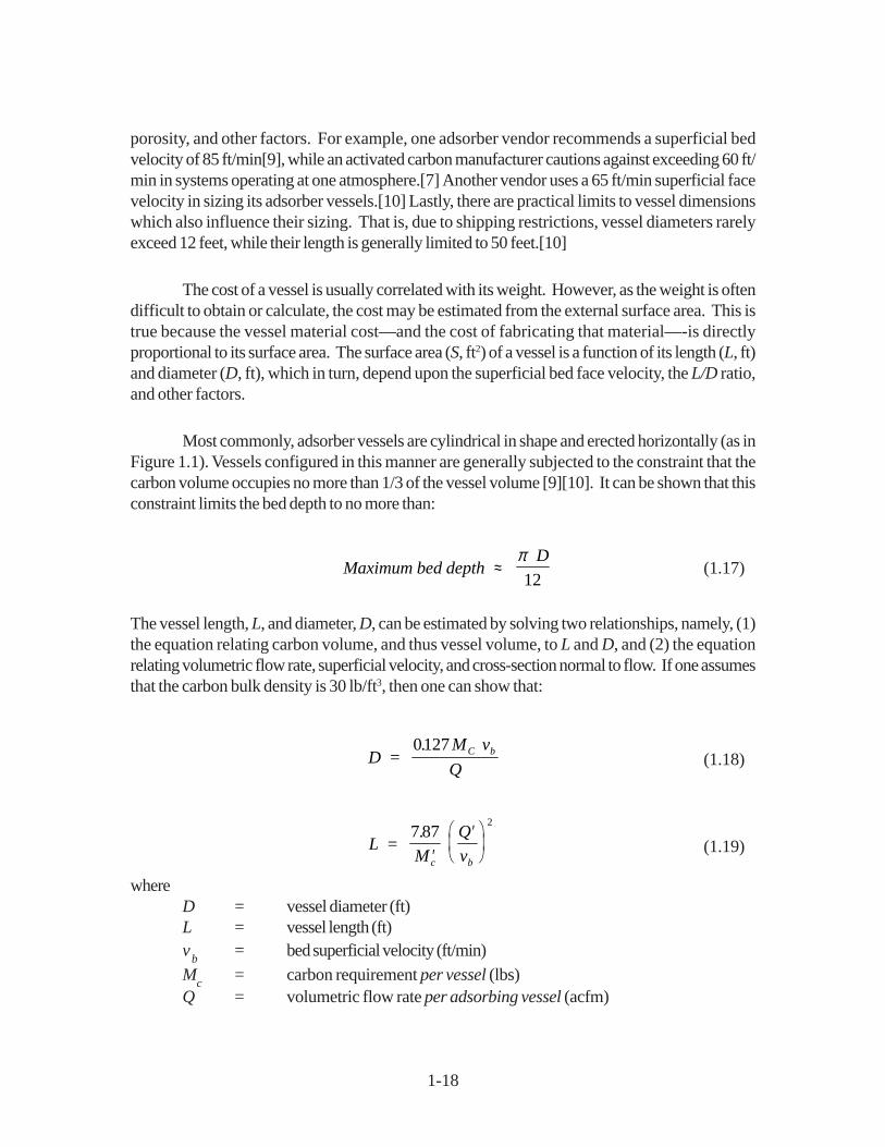
Most commonly, adsorber vessels are cylindrical in shape and erected horizontally (as inFigure 1.1). Vessels configured in this manner are generally subjected to the constraint that thecarbon volume occupies no more than 1/3 of the vessel volume [9][10]. It can be shown that thisconstraint limits the bed depth to no more than:

Maximum bed depthD

≈π12

(1.17)

The vessel length, L, and diameter, D, can be estimated by solving two relationships, namely, (1)the equation relating carbon volume, and thus vessel volume, to L and D, and (2) the equationrelating volumetric flow rate, superficial velocity, and cross-section normal to flow. If one assumesthat the carbon bulk density is 30 lb/ft3, then one can show that:

D M vQ

C b= 0127.

(1.18)

L M

Qvc b

= 7 87

2.

′′

(1.19)

whereD = vessel diameter (ft)L = vessel length (ft)vb = bed superficial velocity (ft/min)Mc = carbon requirement per vessel (lbs)Q = volumetric flow rate per adsorbing vessel (acfm)

1-19

Because the constants in Equations 1.18 and 1.19 are not dimensionless, one must be careful touse the units specified in these equations.

Although other design considerations can result in different values of L and D, theseequations result in L and D which are acceptable from the standpoint of “study” cost estimation forhorizontal, cylindrical vessels which are larger than 2-3 feet in diameter.

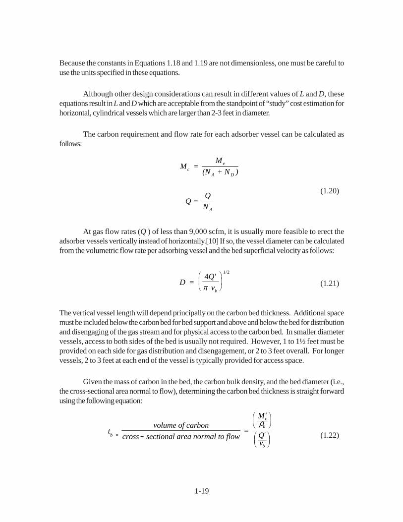
The carbon requirement and flow rate for each adsorber vessel can be calculated asfollows:

M = M

(N + N )

Q = QN

c e

A D

A

(1.20)

At gas flow rates (Q ) of less than 9,000 scfm, it is usually more feasible to erect theadsorber vessels vertically instead of horizontally.[10] If so, the vessel diameter can be calculatedfrom the volumetric flow rate per adsorbing vessel and the bed superficial velocity as follows:

D Qvb

1

= 4

2′

π

/

(1.21)

The vertical vessel length will depend principally on the carbon bed thickness. Additional spacemust be included below the carbon bed for bed support and above and below the bed for distributionand disengaging of the gas stream and for physical access to the carbon bed. In smaller diametervessels, access to both sides of the bed is usually not required. However, 1 to 1½ feet must beprovided on each side for gas distribution and disengagement, or 2 to 3 feet overall. For longervessels, 2 to 3 feet at each end of the vessel is typically provided for access space.

Given the mass of carbon in the bed, the carbon bulk density, and the bed diameter (i.e.,the cross-sectional area normal to flow), determining the carbon bed thickness is straight forwardusing the following equation:

tvolume of carbon

cross sectional area normal to flow =

M

Qv

b =

c

b

b

−

′

′

ρ(1.22)

1-20

where

Db

= carbon bulk density (lb/ft3, assume 30 lb/ft3)

The vessel length is, therefore,

L = t tb a,g+ (1.23)

where

ta,g

= access / gas distribution allowance

= 2 to 6 feet (depending on vertical vessel diameter)

Finally, use the following equation to calculate the surface area of either a horizontal or

vertical vessel:

(1.24)

C Sv

= 2710 778. (1.25)

where

Cv

= vessel cost (fall 1999 $), F.O.B. vender5

and

97 21102≤ ≤S ft (1.25a)

These units would be made of 304 stainless steel, which is the most common material

used in fabricating adsorber vessels. [9][10] However, to obtain the cost of a vessel fabricated

of another material, multiply Cv by and adjustment factor (F

m). A few of these factors are listed

in Table 1.2.

1.3.1.3 Total Purchased Cost

As stated earlier, the costs of such items as the fans, pumps, condenser, decanter,

instrumentation, and internal piping can be factored from the sum of the costs for the carbon and

vessels. Based on four data points derived from costs supplied by an equipment vendor [10],

we found that, depending on the total gas flow rate (Q), the ratio (Rc) of the total adsorber

equipment cost to the cost of the vessels and carbon ranged from 1.14 to 2.24. These data

points spanned a gas flow rate range of approximately 4,000 to 500,000 acfm. The following

regression formula fit these four points:

(1.26)R Q

c = 582

0 133.

.−

5 Two vendors provided information for the 1999 updates, neither felt that modifications to the capital costs of adsorber

system between 1989 and 1999 were appropriate. The major change for 1999 was a decreases in the price of carbon.[4][5]

1-21

where

Q is in the range of 4, 000 to 500,000 acfm

Correlation coefficient (r) = 0.872

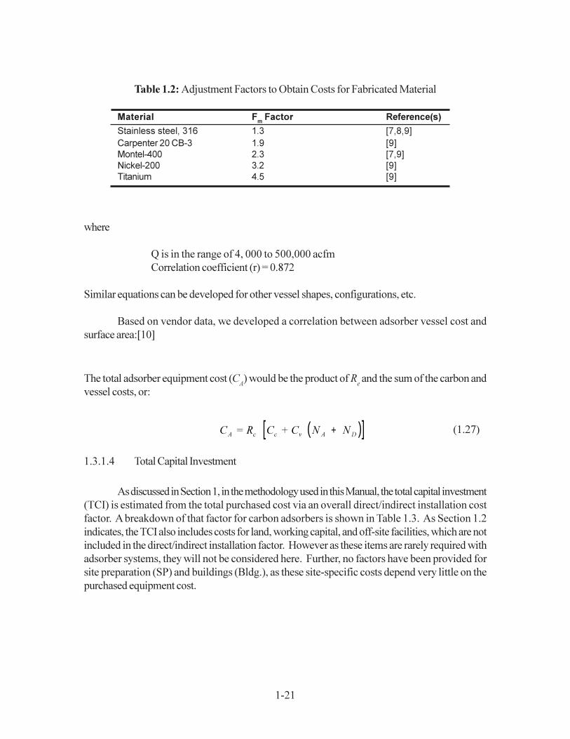
Similar equations can be developed for other vessel shapes, configurations, etc.

Based on vendor data, we developed a correlation between adsorber vessel cost and

surface area:[10]

The total adsorber equipment cost (CA) would be the product of R

e and the sum of the carbon and

vessel costs, or:

( )[ ]C = R C + C N NA c c v A D

+ (1.27)

1.3.1.4 Total Capital Investment

As discussed in Section 1, in the methodology used in this Manual, the total capital investment

(TCI) is estimated from the total purchased cost via an overall direct/indirect installation cost

factor. A breakdown of that factor for carbon adsorbers is shown in Table 1.3. As Section 1.2

indicates, the TCI also includes costs for land, working capital, and off-site facilities, which are not

included in the direct/indirect installation factor. However as these items are rarely required with

adsorber systems, they will not be considered here. Further, no factors have been provided for

site preparation (SP) and buildings (Bldg.), as these site-specific costs depend very little on the

purchased equipment cost.

Table 1.2: Adjustment Factors to Obtain Costs for Fabricated Material

Material Fm Factor Reference(s)

Stainless steel, 316 1.3 [7,8,9]

Carpenter 20 CB-3 1.9 [9]

Montel-400 2.3 [7,9]

Nickel-200 3.2 [9]

Titanium 4.5 [9]

1-22

Direct CostsPurchased equipment costs

Adsorber + auxiliary equipmenta As estimated, A

Instrumentationb 0.10 A

Sales taxes 0.03 A

Freight 0.05 A

Purchased equipment cost, PEC B = 1.18 A

Direct installation costs

Foundations & supports 0.08 B

Handling & erection 0.14 B

Electrical 0.04 B

Piping 0.02 B

Insulation 0.01 B

Painting 0.01 B

Direct installation costs 0.30 B

Site preparation As required, SP

Buildings As required, Bldg.

Total Direct Costs, DC 1.30 B + SP + Bldg.

Indirect Costs (installation)

Engineering 0.10 B

Construction and field expenses 0.05 B

Contractor fees 0.10 B

Start-up 0.02 B

Performance test 0.01 B

Contingencies 0.03 B

Total Indirect Costs, IC 0.31 BTotal Capital Investment = DC + IC 1.61 B + SP + Bldg.

Note that the installation factor is applied to the total purchased equipment cost, which

includes the cost of such auxiliary equipment as the stack and external ductwork and such costs as

freight and sales taxes (if applicable). (“External ductwork” is that ducting needed to convey the

exhaust gas from the source to the adsorber system, and then from the adsorber to the stack.

Costs for ductwork and stacks are shown elsewhere in this Manual) Normally, the adjustment

would also cover the instrumentation cost, but this cost is usually included with the adsorber

equipment cost. Finally, note that these factors reflect “average” installation conditions and could

vary considerably, depending upon the installation circumstances.

Table 1.3: Capital Cost Factors for Carbon Adsorbers [11]

a Ductwork and any other equipment normally not included with unit furnished by adsorber vendor.b Instrumentation and controls often furnished with the adsorber, and thus included in the EC.

1-23

1.3.2 Cannister Systems

Once the carbon requirement is estimated using the above procedure, the number of

cannisters is determined. This is done simply by dividing the total carbon requirement (Me) by the

amount of carbon contained by each cannister (typically, 150 lbs.). This quotient, rounded to the

next highest digit, yields the required number of cannisters to control the vent in question.

Costs for a typical cannister (Calgon’s Ventsorb®) are listed in Table 1.4. These costs

include the vessel, carbon, and connections, but do not include taxes, freight, or installation charges.

Note that the cost per unit decreases as the quantity purchased increases. Each cannister contains

Calgon’s “BPL” carbon (4 x 10 mesh), which is commonly used in industrial adsorption. However,

to treat certain VOCs, more expensive specialty carbons (e.g., “FCA 4 x 10”) are needed. These

carbons can increase the equipment cost by 60% or more.[6] As is indicated in the caption of

Table 1.4, these prices are in mid-1999 dollars.

The price of 180 pound carbon cannisters is approximately $700 in small quantities and

approximately $600 (mid -1999 dollars) in larger quantities. [5] Current trends are toward the

use of larger cannisters. Calgon supplies large cannisters of 1,000 to 2,000 pound capacity where

the carbon is typically exchanged in the field. Calgon reports costs per pound of carbon ranging

from $0.50 to $2.00 depending on mesh, activity and type with a conservative median price of

$1.50 per pound. Calgon also reports the widespread use of larger non-regenerable fixed beds

either 12 feet in diameter (113 square feet capable of of handling 6,000 cfm) and 8x20 foot beds

(160 square feet capable of handling 8,000 cfm). These non-regenerable fixed bed absorbers are

usually atmospheric designs made of thin steel with an internal coating to inhibit corrosion. For

1,000 pound cannisters, Calgon reports typical installation costs of $3,200 and equipment costs

of $5,600 and for 2,000 pound cannisters these costs are $4,600 and $7,800 respectively. For

Table 1.4: Equipment Costs (Mid 1999$) for a

Typical Canister Adsorber [5]

Quantity Equipment Costs forEach Piecea in Dollars ($)

1-3 679

4-9 640

10-29 600

30 585

a These costs are F.O.B., Pittsburgh, PA. They do not include taxes and freight charges.

1-24

onsite carbon replacement services, Calgon estimates carbon costs to be $2.00 to $2.50 per

pound for virgin carbon and $1.50 to $1.80 for reactivated carbon. Annual maintenance costs are

reported to range from 3% to 10% of the installed capital costs.

As fewer installation materials and labor are required to install a cannister unit than a fixed-

bed system, the composite installation factor is consequently lower. The only costs required are

those needed to place the cannisters at, and connect them to, the source. This involves a small

amount of piping only; little or no electrical work, painting, foundations, or the like would be

needed. Twenty percent of the sum of the cannister(s) cost, freight charges, and applicable sales

taxes would cover this installation cost.

1.4 Estimating Total Annual Cost

As Section of this Manual explains, the total annual cost is comprised of three components:

direct costs, indirect costs, and recovery credits. These will be considered separately.

1.4.1 Direct Annual Costs

These include the following expenditures: steam, cooling water, electricity, carbon

replacement, operating and supervisor labor, and maintenance labor and materials. Of these, only

electricity and solid waste disposal or carbon replacement/regeneration would apply to the

cannister-type adsorbers.

1.4.1.1 Steam

As explained in Section 1.1, steam is used during the desorption cycle. The quantity of

steam required will depend on the amount of carbon in the vessel, the vessel dimensions, the type

and amount of VOC adsorbed, and other variables. Experience has shown that the steam

requirement ranges from approximately 3 to 4 lbs of steam/lb of adsorbed VOC.[9][10] Using the

midpoint of this range, we can develop the following expression for the annual steam cost:

C m ps voc s

= s

350 103

. × − θ (1.28)

where

Cs = steam cost ($/yr)

s

= system operating hours (h/yr)

mvoc

= VOC inlet loading (lbs/h)

ps

= steam price ($/thous. lbs)

1-25

If steam price data are unavailable, one can estimate its cost at 120% of the fuel cost. For

example, if the local price of natural gas were $5.00/million BTU, the estimated steam price would

be $6.00/million BTU which is approximately $6.00/thousand lbs. (The 20% factor covers the

capital and annual costs of producing the steam.)

1.4.1.2 Cooling Water

Cooling water is consumed by the condenser in which the steam-VOC mixture leaving the

desorbed carbon bed is totally condensed. Most of the condenser duty is comprised of the latent

heat of vaporization ()Hv) of the steam and VOC. As the VOC )H

v are usually small compared

to the steam )Hv, (about 1000 BTU/lb), the VOC )H

v may be ignored. So may the sensible heat

of cooling the water-VOC condensate from the condenser inlet temperature (about 212oF) to the

outlet temperature. Therefore, the cooling water requirement is essentially a function of the steam

usage and the allowable temperature rise in the coolant, which is typically 30o to 40oF.[9] Using

the average temperature rise (35oF), we can write:

C C

p p

cw

s

s

cw= 343. (1.29)

where

Ccw

= cooling water cost ($/yr)

pcw

= cooling water price ($/thous. gal.)

If the cooling water price is unavailable, use $0.15 to $0.30/thousand gallons.

1.4.1.3 Electricity

In fixed-bed adsorbers, electricity is consumed by the system fan, bed drying/cooling fan,

cooling water pump, and solvent pump(s). Both the system and bed fans must be sized to overcome

the pressure drop through the carbon beds. But, while the system fan must continuously convey

the total gas flow through the system, the bed cooling fan is only used during a part of the desorption

cycle (one-half hour or less).

For both fans, the horsepower needed depends both on the gas flow and the pressure

drop through the carbon bed. The pressure drop through the bed ()Pb) depends on several

variables, such as the adsorption temperature, bed velocity, bed characteristics (e.g., void fraction),

and thickness. But, for a given temperature and carbon, the pressure drop per unit thickness

depends solely on the gas velocity. For instance, for Calgon’s “PCB” carbon (4 x 10 mesh), the

following relationship holds:[8]

∆ P

tv v

b

b

b b = + 0 03679 1107 10

4 2. . × −

(1.30)

1-26

where

)Pb/tb

= pressure drop through bed (inches of water/foot of carbon)

vb

= superficial bed velocity (ft/min)

As Equation 1.22 shows, the bed thickness (tb, ft) is the quotient of the bed volume (V

b)

and the bed cross-sectional area (Ab). For a 30 lb/ft3 carbon bed density, this becomes:

t = V

A

M

Ab

b

b

c

b

= 0 0333. ′

(1.31)

(For vertically erected vessels, Ab = Q /v

b, while for horizontally erected cylindrical vessels, A=

LD.) Once )Pb is known, the system fan horsepower requirement (hp

sf) can be calculated:

hp Q Psf s = 2 50 104

. × − ∆ (1.32)

where

Q = gas volumetric flow through system (acfm)

)Ps

= total system pressure drop = )Pb + 1

(The extra inch accounts for miscellaneous pressure losses through the external ductwork and

other parts of the system.[9]6 However, if extra long duct runs and/or preconditioning equipment

are needed, the miscellaneous losses could be much higher.)

This equation incorporates a fan efficiency of 70% and a motor efficiency of 90%, or 63%

overall.

The horsepower requirement for the bed drying/cooling fan (hpcf) is computed similarly.

While the bed fan pressure drop would still be )Pb, the gas flow and operating times would be

different. For typical adsorber operating conditions, the drying/cooling air requirement would be

50 to 150 ft3/lb carbon, depending on the bed moisture content, required temperature drop, and

other factors. The operating time (2cf) would be the product of the drying/cooling time per desorption

cycle and the number of cycles per year. It can be shown that:

θ θθ

θcf D

A s

A

N = 0 4.

(1.33)

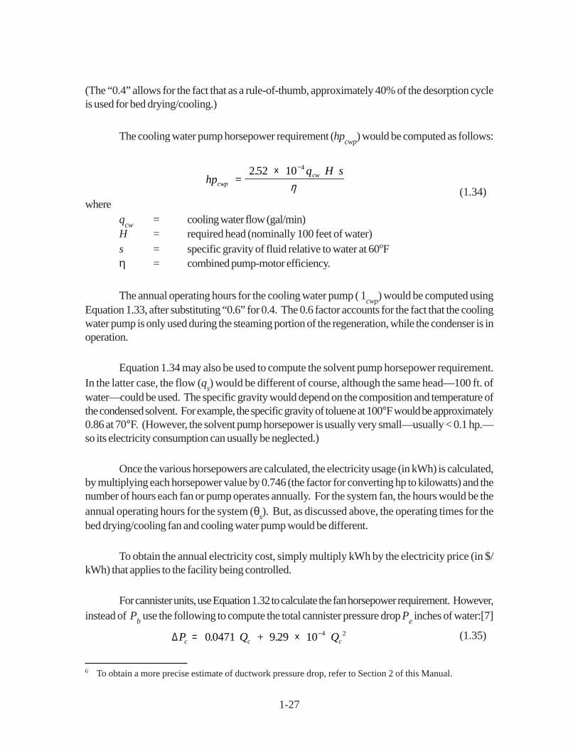
1-27

(The “0.4” allows for the fact that as a rule-of-thumb, approximately 40% of the desorption cycleis used for bed drying/cooling.)

The cooling water pump horsepower requirement (hpcwp) would be computed as follows:

hpq H s

cwpcw =

2 52 10 4. × −

η (1.34)where

qcw = cooling water flow (gal/min)H = required head (nominally 100 feet of water)s = specific gravity of fluid relative to water at 60oFη = combined pump-motor efficiency.

The annual operating hours for the cooling water pump ( 1cwp) would be computed usingEquation 1.33, after substituting “0.6” for 0.4. The 0.6 factor accounts for the fact that the coolingwater pump is only used during the steaming portion of the regeneration, while the condenser is inoperation.

Equation 1.34 may also be used to compute the solvent pump horsepower requirement.In the latter case, the flow (qs) would be different of course, although the same head—100 ft. ofwater—could be used. The specific gravity would depend on the composition and temperature ofthe condensed solvent. For example, the specific gravity of toluene at 100°F would be approximately0.86 at 70°F. (However, the solvent pump horsepower is usually very small—usually < 0.1 hp.—so its electricity consumption can usually be neglected.)

Once the various horsepowers are calculated, the electricity usage (in kWh) is calculated,by multiplying each horsepower value by 0.746 (the factor for converting hp to kilowatts) and thenumber of hours each fan or pump operates annually. For the system fan, the hours would be theannual operating hours for the system (θs). But, as discussed above, the operating times for thebed drying/cooling fan and cooling water pump would be different.

To obtain the annual electricity cost, simply multiply kWh by the electricity price (in $/kWh) that applies to the facility being controlled.

For cannister units, use Equation 1.32 to calculate the fan horsepower requirement. However,instead of Pb use the following to compute the total cannister pressure drop Pe inches of water:[7]

∆ P Q Qc c c= × − + 0 0471 9 29 10 4 2. . (1.35)

6 To obtain a more precise estimate of ductwork pressure drop, refer to Section 2 of this Manual.

1-28

where

Qc = flow through the cannister (acfm).

1.4.1.4 Carbon Replacement

As discussed above, the carbon has a different economic life than the rest of the adsorbersystem. Therefore, its replacement cost must be calculated separately. Employing the proceduredetailed in Section 1, we have:

( )CRC = CRF C Cc c c cl108. + (1.36)

where

CRFc = capital recovery factor for the carbon1.08 = taxes and freight factorCc, Ccl = initial cost of carbon (F.O.B. vendor) and carbon replacement labor

cost, respectively ($)

The replacement labor cost covers the labor cost for removing spent carbon from vesselsand replacing it with virgin or regenerated carbon. The cost would vary with the amount of carbonbeing replaced, the labor rates, and other factors. For example, to remove and replace a 50,000pound carbon charge would require about 16 person-days, which, at typical wage rates, is equivalentto approximately $0.05/lb replaced.[13]

A typical life for the carbon is five years. However, if the inlet contains VOCs that are verydifficult to desorb, tend to polymerize, or react with other constituents, a shorter carbon lifetime—perhaps as low as two years—would be likely.[1] For a five-year life and 7% interest rate, CRFc= 0.2439.

1.4.1.5 Solid Waste Disposal

Disposal costs are rarely incurred with fixed-bed adsorbers, because the carbon is almost alwaysregenerated in place, not discarded. The carbon in cannister units should also be regenerated inmost cases. For larger vessels, common practice is for a carbon vendor to pick up the spentcarbon and replace it with fresh carbon. The spent carbon is then returned to a central facility forregeneration. EPA encourages both solvent recovery and reuse of spent carbon as pollutionprevention and waste minimzation techniques.

1-29

In some cases, the nature of the solvents, including their extremely hazardous nature or the difficulty

in desorbong them from the carbon may make disposal the preferred option. In these cases, an

entire cannister—carbon, drum, connections, etc.— may be shipped to a secure landfill. The cost

of landfill disposal could vary considerably, depending on the number of cannisters disposed of,

the location of the landfill, etc. Based on data obtained from two large landfills, for instance, the

disposal cost would range from approximately $35 to $65 per cannister excluding transportation

costs.[14][15]

1.4.1.6 Operating and Supervisory Labor

The operating labor for adsorbers is relatively low, as most systems are automated and

require little attention. One-half operator hour per shift is typical.[12] The annual labor cost would

then be the product of this labor requirement and the operating labor wage rate ($/h) which,

naturally, would vary according to the facility location, type of industry, etc. Add to this 15% to

cover supervisory labor, as Section 1.2 suggests.

1.4.1.7 Maintenance Labor and Materials

Use 0.5 hours/shift for maintenance labor [12] and the applicable maintenance wage rate.

If the latter data are unavailable, estimate the maintenance wage rate at 110% of the operating

labor rate, as Section 1 suggests. Finally, for maintenance materials, add an amount equal

to the maintenance labor, also per Section 1.

1.4.2 Indirect Annual Costs

These include such costs as capital recovery, property, taxes, insurance, overhead, and

administrative costs (“G&A”). The capital recovery cost is based on the equipment lifetime and

the annual interest rate employed. (See Section 1.2 for a thorough discussion of the capital recovery

cost and the variables that determine it.) For adsorbers, the system lifetime is typically ten years,

except for the carbon, which, as stated above, typically needs to be replaced after five years.

Therefore, when figuring the system capital recovery cost, one should base it on the installed

capital cost less the cost of replacing the carbon (i.e., the carbon cost plus the cost of labor

necessary to replace it). Substituting the initial carbon and replacement labor costs from Equation

1.36, we obtain:

( )[ ]CRC TCI C + C CRFs c cl s

= - 108. (1.37)

1-30

where

CRCs

= capital recovery cost for adsorber system ($/yr)

TCI = total capital investment ($)

1.08 = taxes and freight factor

Cc,Ccl

= initial carbon cost (F.O.B. vendor) and carbon replacement cost,

respectively ($)

CRFs

= capital recovery factor for adsorber system (defined in Section 1. 2).

For a ten-year life and a 7% annual interest rate, the CRFs would be 0.1424.

As Section 1.2 indicates, the suggested factor to use for property taxes, insurance, and

administrative charges is 4% of the TCI. Finally, the overhead is calculated as 60% of the sum of

operating, supervisory, and maintenance labor, and maintenance materials.

The above procedure applies to cannister units as well, except in those case where the

entire unit and not just the carbon is replaced. The piping and ducting cost can usually be considered

a capital investment with a useful life of ten years. However, whether the cannister itself would be

treated as a capital or an operating expense would depend on the particular application and would

need to be evaluated on a case-by-case basis.

1.4.3 Recovery Credits

These apply to the VOC which is adsorbed, then desorbed, condensed, and separated

from the steam condensate. If the recovered VOC is sufficiently pure, it can be sold. However, if

the VOC layer contains impurities or is a mixture of compounds, it would require further treatment,

such as distillation. Purification and separation costs are beyond the scope of this chapter. Needless

to say, the costs of these operations would offset the revenues generated by the sale of the VOC.

Finally, as an alternative to reselling it, the VOC could be burned as fuel and valued accordingly. In

any case, the following equation can be used to calculate these credits:

RC = m P Evoc s voc

θ (1.38)

where

RC = recovery credit ($/yr)

mvoc

= VOC inlet loading (lbs/h)

2s

= system operating hours (h/yr)

pvoc

= resale value of the recovered VOC ($/lb)

E = adsorber VOC control efficiency

1-31

By definition, the efficiency (E) is the difference between the inlet and outlet VOC mass

loading, divided by the inlet loading. However, during an adsorption cycle the outlet VOC loading

will increase from essentially zero at the start of the cycle to the breakthrough concentration at the

end of the cycle. Because the efficiency is a function of time, it should be calculated via integration

over the length of the adsorption cycle. To do this would require knowledge of the temporal

variation of the outlet loading during the adsorption cycle. If this knowledge is not available to the

Manual user, a conservative approximation of the efficiency may be made by setting the outlet

loading equal to the breakthrough concentration.

1.4.4 Total Annual Cost

Finally, as explained in Section 1, the total annual cost (TAC) is the sum of the direct and

indirect annual costs, less any recovery credits, or:

TAC = DC + IC - RC (1.39)

1.4.5 Example Problem

A source at a printing plant emitting 100 lb/h of toluene is to be controlled by a carbon

adsorber. The plant proposes to operate the adsorber in a continuous mode for 8,640 h/yr (360

days). While operating, two carbon beds will be adsorbing, while a third will be desorbing/on

stand by. For its convenience, the plant has selected adsorption and desorption times of 12 and 5

hours, respectively. The total waste gas flow is 10,000 acfm at the adsorber inlet conditions (one

atmosphere and 77oF). The waste gas contains negligible quantities of particulate matter and

moisture. Further, the applicable VOC regulation requires the adsorber to achieve a mean removal

efficiency of 98% during the entire adsorption cycle. Finally, assume that the recovered toluene is

recycled at the source. Estimate the total capital investment and total annual cost for the adsorber

system.

Carbon Working Capacity: At the stated flow and pollutant loading, the toluene inlet concentration

is 710 ppm. This corresponds to a partial pressure of 0.0104 psia. Substituting this partial

pressure and the toluene isotherm parameters (from Table 1) into Equation 1, we obtain an equilibrium

capacity of 0.333 lb/lb. By applying the rule-of-thumb discussed above (page 4-19), we obtain a

working capacity of 0.167 lb/lb (i.e., 0.333/2).

Carbon Requirement: As stated above, this adsorber would have two beds on-line and a third

off-line. Equation 3.12 can answer this question. Substitution of the adsorption time and numbers

of adsorbing and desorbing beds yields:

Desorption timeN

Nh h

D A

D

A

= θ θ≤

= × =12 05 6.

1-32

Because the stated desorption time (5 hours) is less than 6 hours, the proposed bed configuration

is feasible. Next, calculate the carbon requirement (Mc) from Equation 3.14:

( ) ( )M

m

w

N

N

lb h h

lb lblbs

c

voc

c

A

D

A

= +

=

× × +=θ 1

100 12 1 05

016710800

.

.,

From Equation 3.16, the carbon cost is:

C Mc c

= =100 800. $10,

Adsorber Vessel Dimensions: Assume that the vessels will be erected horizontally and select a

superficial bed velocity (vb) of 75 ft/min. Next, calculate the vessel diameter (D), length (L), and

surface area (S) from Equations 3.18, 3.19, and 3.24, respectively. [Note: In these equations, Mc

= Mc (N

A + N

D) = 3,600 lb and Q = Q/N

A = 5,000 acfm.]

( ) ( )D

M v

Qft

e b=′

= =0127 0127 3 600 75

5 000686

. . ,

,.

LM

Q

vft

c b

=′

′

=

=

787 787

3 600

5 000

759 72

2 2

. .

,

,.

S D LD

ft= +

=π

2283

Because S falls between 97 and 2,110 ft2, Equation 1.25 can be used to calculate the cost per

vessel, Cv (assuming 304 stainless steel construction). Thus:

C Sv

= =271 9000 778.

$21,

Adsorber Equipment Cost: Recall that the adsorber equipment cost is comprised of the adsorber

vessels, carbon, and the condenser, decanter, fan, pumps and other equipment usually included in

the adsorber price. The cost of the latter items are “factored” from the combined cost of the

vessels and carbon. Combining Equations 1.26 and 1.27, we have:

( )[ ]C Q C N N CA c A D v

= + +−582

0133.

.

1-33

Substitution of the above values yields:

CA' $130,800

Cost of Auxiliary Equipment: Assume that costs for the following auxiliary equipment have

been estimated from data in other parts of the Manual:

Ductwork $16,500

Dampers 7,200

Stack 8,500

Total $32,000

Total Capital Investment: The total capital investment is factored from the sum of the adsorber

unit and auxiliary equipment cost, as displayed in Table 1.5. Note that no line item cost has been

shown for instrumentation, for this cost is typically included in the adsorber price.

Therefore:

Purchased Equipment Cost = “B” = 1.08 x “A”= 1.08 x ($130,800 + $32,200) = $176,040

And:

Total Capital Investment (rounded) = 1.61 x “B” = $283,400

Annual Costs: Table 1.5 gives the direct and indirect annual costs for the carbon adsorber

system, as calculated from the factors in Section 1.1.4. Except for electricity, the calculations in

the table show how these costs were derived. The following discussion will deal with the electricity

cost.

First, recall that the electricity includes the power for the system fan, bed drying/cooling

fan, and the cooling water pump. (The solvent pump motor is normally so small that its power

consumption may be neglected.) These consumptions are calculated as follows:

System fan is calculated from Equation 1.32:

kWh kW hp Q Psf s s= × × −0746 250 10

4. ∆ θ

1-34

Table 1.5: Capital Cost Factors for Carbon Adsorber System Example Problem

Cost Item Factor

Direct Costs

Purchased equipment costs

Adsorber vessels and carbon $130,800

Auxiliary equipment 32,200

Sum = A $163,000

Instrumentation, 0.1 A

Sales taxes, 0.03 A 4,890

Freight, 0.05 A 8,150

Purchased equipment cost, PEC $176,040

Direct installation costs

Foundations & supports, 0.08 B 14,083

Handling & erection, 0.14 B 24,646

Electrical, 0.04 B 7,042

Piping, 0.02 B 3,521

Insulation for ductwork, 0.01 B 1,760

Painting, 0.02 B 1,760

Direct installation costs $52,812

Site preparation

Buildings

Total Direct Costs, DC $228,852

Indirect Costs (installation)

Engineering, 0.10 B 17,604

Construction and field expenses, 0.05 B 8,802

Contractor fees, 0.10 B 17,604

Start-up, 0.02 B 3,521

Performance test, 0.01 B 1,760

Contingencies, 0.03 B 5,281

Total Indirect Costs, IC $54,572

Total Capital Investment (rounded) $283,400 a

The cost for this is included in the adsorber equipment cost.

1-35

But:

( ) ( )∆ ∆P inches water P t v vs s b b b

= + = + × +−1 003679 1107 10 1

4 2. .

(The latter expression was derived from Equation 1.30, assuming that the carbon used in this

example system is Calgon’s “PCB”, 4 x 10 mesh size.)

By assuming a carbon bed density, of 30 lb/ft3, Equation 1.31 can be used to calculate the bed

thickness (tb):

Bed thickness tM

A

M

LDft

b

c

b

c= =′

=′

=00333 00333

180. .

.

Thus:

( )∆P inchess

= + × + × × =−1 180 003679 75 1107 10 75 7 09

4 2. . . .

and finally:

kWh in acfm h yr

kWh yr

sf = × × × × ×

=

−0746 25 10 7 09 10 000 8 640

114 200

4. . . . , ,

,

Bed drying/cooling fan: During the drying/cooling cycle, the pressure drop through the bed also

equals Pb. However, as Section 1.4.1.3 indicates, the flow and operating time are different. For

the air flow, take the midpoint of the range (100 ft3 air/lb carbon) and divide by 2 hours (the bed

drying/cooling time), yielding: 100 ft3/lb x 3,600 lbs x 1/120 min = 3,000 acfm. Substituting this

into Equation 1.32 results in:

250 10 7 09 3 000 5324

. . , .× × × =− inches acfm hp

From Equation 1.33, we get:

Θ cf hh

hh= × × × =04 5 2

8 640

1212.

,

1-36

Thus:

kWh kW hp hp h kWh yrcf = × × =0746 532 2 880 11400. . , ,

Cooling water pump: The cooling water pump horsepower is calculated from Equation 1.34.

Here, let = 63% and H = 100 ft. The cooling water flow (qcw

) is the quotient of the annual cooling

water requirement and the annual pump operating time. From the data in Table 1.6, we obtain the

cooling water requirement: 10,400,000 gal/yr. The pump annual operating time is obtained from

Equation 1.33 (substituting 0.6 for 0.4), or cwp = (0.6)(5 h)(2)(8,640)/12 = 4,320 h/yr.

Thus:

( ) ( )hp

ft gal yr

h yr min yrhp

cwp=

××

×=

−252 10 100

063

10 400 000

4 320 60160

4.

.

, ,

,.

Thus:

( ) ( )hp

ft gal yr

h yr min yrhp

cwp=

××

×=

−252 10 100

063

10 400 000

4 320 60160

4.

.

, ,

,.

And:

kWh kW h hp h yr kWh yrcwp

= × × =0746 160 4 320 5160. . , ,

Summing the individual power consumptions, we get the value shown in Table 1.5:

131,000kWh/yr

Recovery Credit: As Table 3.6 indicates, a credit for the recovered toluene has been taken.

However, to account for miscellaneous losses and contamination, the toluene is arbitrarily valued

at one-half the November 1989 market price of $0.0533/lb(= $111/ton).[16]

Total Annual Cost: The sum of the direct and indirect annual costs, less the toluene recovery

credit, yields a net total annual cost of $76,100. Clearly, this “bottom line” is very sensitive to the

recovery credit and, in turn, the value given the recovered toluene. For instance, if it had been

valued at the full market price ($221/ton), the credit would have doubled and the total annual cost

would have been $29,200. Thus when incorporating recovery credits, it is imperative to select the

value of the recovered product carefully.

1-37

Cost Item Calculations Cost

Direct Annual Costs, DC Operating Labor Operator 0.5h/shift x 3 shifts/day x 360 days/yr x $12/hr $6,480 Supervisor 15% of operator = 0.15 x 6,480 970 Operating materials Maintenance Labor 0.5h/shift x 3 shifts/day x 360 days/yr x $13.20/hr 7,130 Material 100% of maintenance labor 7,130 Replacement Parts, Carbon (5-year life) Replacement Labor 0.2439 ($0.05/lb x 10,800 lb) 130 Carbon Cost

a 0.2439 ($21,600 x 1.08) 5,690

Utilities Electricity $0.06 kWh x 131,000 kWh/yr 7,860 Steam 3.5 lb/lb VOC x $6/103 x 100 lb VOC/hr x 8,640

hr/yr 18,140

Cooling Water 3.43 gal/lb steam x [(3.5 x 100 x 8,640) lb steam x $0.20/103 gal.] / yr

2,070

Total DC $55,600 Indirect Annual Costs, IC Overhead 60% of sum of operating labor, maintenance

labor, & maintenance materials = 0.6 (6,480 + 970 + 7,130 + 7,130)

13,030

Administrative charges 2% of Total Capital Investment = 0.02 ($316,000) 6,320 Property tax 1% of Total Capital Investment = 0.01 ($316,000) 3,160 Insurance 1% of Total Capital Investment = 0.01 ($316,000) 3,160 Capital recovery

b 0.1424 [316,000 - 0.05 (10,800) - 1.08 (21,600)] 41,600

Total IC $67,270 Recovery Credit (toluene) (46,820)

Total Annual Cost (rounded) $76,100 a The 1.08 factor is for freight and sales taxes.

b The capital recovery cost factor, CRF, is a function of the adsorber or equipment life and the

opportunity cost of the capital (i.e., interest rate). For example, for a 10 year equipment life and a 7% interest rate, CRF = 0.1424.

Table 1.6: Annual Costs for Carbon Adsorber Systems, Example Problem

1-38

References

[1 Correspondence: Robert L. Stallings and William Klotz (Research Triangle Institute,

Research Triangle Park, NC) to William M. Vatavuk (U.S. EPA, OAQPS, Research

Triangle Park, NC), June 24, 1986.

[2] Calvert, Seymour and Englund, Harold M. (eds.), Handbook of Air Pollution Control

Technology, John Wiley & Sons, New York, 1984, pp. 135-192.

[3] Handbook of Chemistry and Physics, 54th Edition, The Chemical Rubber Company,

Cleveland, 1973-74, pp. D85-D92.

[4] Correspondence: Wayne G. Schulinger and Georgiana Riley (TIGG Corporation,

Pittsburgh, PA) to Janet Groeber (SAIC, Cincinnati, OH), October11,1 999.

[5] Correspondence: Mark H. Stenzel (Calgon Carbon Corporation, Pittsburgh, PA) to

Janet Groeber (SAIC, Cincinnati, OH), August 24,1 999.

[6] “Calgon Ventsorb® for Industrial Air Purification” (Bulletin 23-56a), Calgon Corporation,

Pittsburgh, 1986.

[7] Adsorption Handbook, Calgon Corporation, Pittsburgh, 1980.

[8] Rogers, Tony, “Comparison of BED SIZE and Calgon Adsorption Isotherms”, Research

Triangle Institute (Research Triangle Park, NC), January 20, 1988.

[9] Correspondence: Richard Selznick (Baron Blakeslee, Inc., Westfield. NJ) to William

M. Vatavuk (U.S. EPA, OAQPS, Research Triangle Park, NC), April 23, 1986.

[10] Correspondence: Denny Clodfelter(M&W Industries, Inc., Rural Hall, NC) to William

M. Vatavuk (U.S. EPA, OAQPS, Research Triangle Park, NC), September 25, 1989.

[11] Matley, Jay (ed.), Modern Cost Engineering, McGraw-Hill Publications Co., New

York, 1984, p. 142.

[12] Vatavuk, William M. and Neveril, Robert, “Estimating Costs of Air Pollution Control

Systems, Part II: Factors for Estimating Capital and Operating Costs,” Chemical

Engineering, November 3, 1980, pp. 157-162.

1-39

[13] Telephone conversation: Robert L. Stallings (Research Triangle Institute, Research Triangle

Park, NC) with William M. Vatavuk (U.S. EPA, OAQPS, Research Triangle Park, NC),

September 11, 1986.

[14] Correspondence: William Kitto (Chemwaste, Sulphur, LA) to William M. Vatavuk (U.S.

EPA, OAQPS, Research Triangle Park, NC), July 25, 1986.

[15] Correspondence: Jerry Locklear (GSX, Pinewood, SC) to William M. Vatavuk (U.S.

EPA, OAQPS, Research Triangle Park, NC), July 25, 1986.

[16] Chemical Marketing Reporter, December 2, 1989.

TECHNICAL REPORT DATA

(Please read Instructions on reverse before completing)

1. REPORT NO.

452/B-02-0012. 3. RECIPIENT'S ACCESSION NO.

4. TITLE AND SUBTITLE

The EPA Air Pollution Control Cost Manual

5. REPORT DATE

January, 2002

6. PERFORMING ORGANIZATION CODE

7. AUTHOR(S)

Daniel Charles Mussatti

8. PERFORMING ORGANIZATION REPORT NO.

9. PERFORMING ORGANIZATION NAME AND ADDRESS

U.S. Environmental Protection Agency Office of Air Quality Planning and Standards Air Quality Standards and Strategies Division Innovative Strategies and Economics Group Research Triangle Park, NC 27711

10. PROGRAM ELEMENT NO.

11. CONTRACT/GRANT NO.

12. SPONSORING AGENCY NAME AND ADDRESS

Director Office of Air Quality Planning and Standards Office of Air and Radiation U.S. Environmental Protection Agency Research Triangle Park, NC 27711

13. TYPE OF REPORT AND PERIOD COVERED

Final

14. SPONSORING AGENCY CODE

EPA/200/04

15. SUPPLEMENTARY NOTES

Updates and revises EPA 453/b-96-001, OAQPS Control Cost Manual, fifth edition (in English only)

16. ABSTRACT

In Spanish, this document provides a detailed methodology for the proper sizing and costing of numerous airpollution control devices for planning and permitting purposes. Includes costing for volatile organiccompounds (VOCs); particulate matter (PM); oxides of nitrogen (NOx); SO2, SO3, and other acid gasses;and hazardous air pollutants (HAPs).

17. KEY WORDS AND DOCUMENT ANALYSIS

a. DESCRIPTORS b. IDENTIFIERS/OPEN ENDED TERMS c. COSATI Field/Group

EconomicsCostEngineering costSizingEstimationDesign

Air Pollution controlIncineratorsAbsorbersAdsorbersFiltersCondensersElectrostatic PrecipitatorsScrubbers

18. DISTRIBUTION STATEMENT

Release Unlimited

19. SECURITY CLASS (Report)

Unclassified21. NO. OF PAGES

1,400

20. SECURITY CLASS (Page)

Unclassified22. PRICE

EPA Form 2220-1 (Rev. 4-77)EPA Form 2220-1 (Rev. 4-77) PREVIOUS EDITION IS OBSOLETE