secondarycirculationingranularflowthrough...

SECONDARY CIRCULATION IN GRANULAR FLOW THROUGHNONAXISYMMETRIC HOPPERS∗

PIERRE A. GREMAUD† , JOHN V. MATTHEWS‡ , AND DAVID G. SCHAEFFER§

SIAM J. APPL. MATH. c© 2003 Society for Industrial and Applied MathematicsVol. 64, No. 2, pp. 583–600

Abstract. Jenike’s radial solution, widely used in the design of materials-handling equipment,is a similarity solution of steady-state continuum equations for the flow under gravity of granularmaterial through an infinite, right-circular cone. In this paper we study how the geometry of thehopper influences this solution. Using perturbation theory, we compute a first-order correction tothe (steady-state) velocity resulting from a small change in hopper geometry, either distortion of thecross section or tilting away from vertical. Unlike for the Jenike solution, all three components ofthe correction velocity are nonzero; i.e., there is secondary circulation in the perturbed flow.

Key words. granular, similarity solution, perturbation theory

AMS subject classifications. 65L80, 35J65, 76T25

DOI. 10.1137/S0036139903415124

1. Introduction. In manufacturing industries, raw materials are stored in gran-ular form in a silo, and when needed, they are expected to flow out of the silo undergravity through a hopper. Problems in the discharge process are frequent and expen-sive; see, e.g., [8]. As demonstrated by a Rand Corporation study [9], these problemsare symptomatic of our poor understanding of the behavior of granular materials.1

Jenike’s radial solution is a central component of silo design. Despite its impor-tance, this solution is subject to many severe restrictions:

1. Granular material is modeled as a continuum, with an ad hoc constitutive law.2. The flow is assumed to be steady.3. The flow domain, a mathematical idealization, is an infinite cone, given in

spherical polar coordinates by the formula

(r, θ, φ) : 0 < r < ∞, 0 ≤ θ < θw (θw = constant).

4. Only similarity solutions are considered.

∗Received by the editors July 7, 2003; accepted for publication (in revised form) July 22, 2003;published electronically December 31, 2003.

http://www.siam.org/journals/siap/64-2/41512.html†Department of Mathematics and Center for Research in Scientific Computation, North Carolina

State University, Raleigh, NC 27695-8205 ([email protected]). The research of this authorwas partially supported by the Army Research Office through grant DAAD19-99-1-0188 and by theNational Science Foundation through grant DMS-9818900.

‡Department of Mathematics, Duke University, Durham, NC 27708-0320 ([email protected]). The research of this author was partially supported by the National Science Foundationthrough grant DMS-9983320.

§Department of Mathematics and Center for Nonlinear and Complex Systems, Duke University,Durham, NC 27708-0320 ([email protected]). The research of this author was partially supportedby the National Science Foundation through grant DMS-9803305.

1The study compared the design output and the actual output of a total of 60 manufacturingplants in various industries, 22 that were based primarily on liquids-processing technology and 38 onsolids-processing technology. On average, the liquids-processing plants produced at 84% of designcapacity while the solids-processing plants produced at only 63% of design capacity. To quote Merrow[9], “In economic terms, the difference between 63% of design and 84% is very large. It implies acapital cost per unit of output about one-third higher for the solids-processing plants, on the basis ofpoor performance alone. In addition, poor performance is inevitably associated with higher operatingand maintenance costs per unit of product.” Moreover, the standard deviation of the solids-processingdata set was much greater, indicative of our difficulties in predicting the behavior of granular solids.

583

584 PIERRE A. GREMAUD, JOHN V. MATTHEWS, DAVID G. SCHAEFFER

In this paper we relax restrictions 3 and 4 partly. Specifically, we generalize thedomain to an infinite pyramidal hopper described by the inequality

0 ≤ θ < θw + ε cosmφ,(1.1)

where ε is a small parameter and m is a positive integer. Assuming a perturbationseries

v(0) + εv(1) + · · ·for the flow velocity in the domain (1.1), where v(0) is Jenike’s solution, we derivea linear PDE for the first-order correction v(1). The r-dependence of v(1) still hassimilarity form, and the φ-dependence may be handled by separation of variables. Inthis way we reduce solving the PDE for v(1) to solving a two-point boundary problemon the interval 0 < θ < θw.

In Jenike’s solution, only the radial component v(0)r of the velocity is nonzero. By

contrast, all three components of the correction velocity v(1) are nonzero. In otherwords, distortion of the conical domain leads to secondary circulation. For example,in Figure 5.1 below, the flow in the θ, φ-directions is shown for a circular hopper thatis tilted slightly to the right, and in Figure 5.2, for a slightly distorted vertical hopper.

Circulation was previously observed by Williams and Rege in discrete elementsimulations of granular systems [11], [13]. While a connection between such time-dependent, discrete simulations and the steady-state continuum theory below is un-clear, the similarities are uncanny. Both find a secondary circulation in essentiallytwo-dimensional granular systems undergoing a uniform compression.

The outline of the paper is as follows. In section 2, the governing equations arerecalled together with Jenike’s construction of similarity solutions in conical domains.For nonaxisymmetric domains of the type (1.1), the problem is then linearized aboutJenike’s solution in section 3. The resulting system is discretized in section 4. Nu-merical results and discussion are offered in section 5.

2. The model.

2.1. Governing equations and boundary conditions. The unknowns arethe 3-component velocity vector v, the 3× 3 symmetric stress tensor T , and a scalarplasticity coefficient λ. (The density ρ is a constant.) In total, there are 3 + 6 + 1 =10 unknown functions. In writing the equations for these variables, we need thestrain rate tensor V = −1/2(∇v +∇vT ) and the deviatoric part of the stress tensordev T = T − 1

3 (trT ) I. Note the sign convention: V measures the compression rate ofthe material; analogously, positive eigenvalues of T correspond to compressive stresses.This sign convention reflects the fact that granular materials disintegrate under tensilestresses.

Following [12], we require that these variables satisfy

∇ · T = ρ g,(2.1)

V = λ dev T,(2.2)

|dev T |2 = 2s2(trT /3)2,(2.3)

where g is the (vector) acceleration of gravity, | · | denotes the Frobenius norm

|T |2 =

3∑i,j=1

T 2ij = trT 2

NONAXISYMMETRIC GRANULAR FLOW 585

(the latter equality only for symmetric tensors), and s = sin δ, with δ being the an-gle of internal friction of the material under consideration (see [10]). Equation (2.1)expresses force balance; i.e., Newton’s second law with inertia neglected because theflow is assumed slow; it is equivalent to three scalar equations. Equations (2.2) and(2.3) are constitutive laws, the alignment condition and the von Mises yield condi-tion, respectively; they are equivalent to six and to one scalar equations, respectively.Thus (2.1)–(2.3) is a determined system, ten equations for ten unknowns. Since (2.3)contains no derivatives, this system has a differential-algebraic character. Taking thetrace of (2.2), we see that div v = −trV = 0; thus, incompressibility is part of theconstitutive assumptions. Incidentally, for a solution to be physical, the function λin (2.2) must satisfy λ ≥ 0 everywhere; otherwise, friction would be adding energyto the system rather than dissipating it. In fact, we want λ to be strictly positivesince one of the assumptions underlying the derivation of (2.1)–(2.3) is that materialis actually deforming.

We seek solutions of (2.1)–(2.3) in a pyramidal domain, expressed in sphericalpolar coordinates as

Ω = (r, θ, φ) : 0 ≤ θ < C(φ),(2.4)

where C is a given smooth 2π-periodic function. Such a domain represents a mathe-matical idealization of a converging hopper, in general, a nonaxisymmetric one.

On the boundary ∂Ω = (r, C(φ), φ), wall impenetrability imposes one boundarycondition on the velocity; i.e.,

vN = 0,(2.5)

where vN is the normal velocity. Two additional boundary conditions come fromCoulomb’s law of sliding friction. The surface traction τ—i.e., the force exerted bythe wall on the material—is given by

τi =

3∑j=1

TijNj ,

where N is the unit interior normal to ∂Ω. If the vector τ has normal component τNand tangential component τT = τ − τNN , then we require that

τT = −µw τN (v/|v|),(2.6)

where µw is the coefficient of friction between the wall and the material. Note thefollowing: (i) If T is positive definite (i.e., if all stresses are compressive), then τN > 0.(ii) While τN is a scalar, τT is effectively a two-component vector; thus, (2.6) isequivalent to two scalar equations. (iii) Because of (2.5), the velocity v is tangentialto ∂Ω; we are assuming that v = 0 at the boundary.

2.2. Jenike’s similarity solution. Suppose that the domain (2.4) is axisym-metric; i.e., suppose

Ω = (r, θ, φ) : 0 ≤ θ < θw,(2.7)

where θw is a constant. In this case Jenike [7] found that (2.1)–(2.3) have solutionsthat are independent of φ and have a similarity dependence on r,

v(0)(r, θ) = r−2 v(0)(θ), T (0)(r, θ) = r T (0)(θ).(2.8)


(Here and below, a hat above a variable indicates a function that depends on θ alone.)

Moreover, only the radial component of velocity is nonzero; i.e., v(0)θ = v

(0)φ = 0.

Similarly, T(0)rφ = T

(0)θφ = 0. Indeed, all components of T can be expressed in terms of

two scalar variables, the so-called Sokolovskii variables [10]: the mean stress p(0) =trT (0) /3 and an angle ψ; specifically,

dev T (0) = s p(0)

− 2√3cos 2ψ − sin 2ψ 0

− sin 2ψ 1√3cos 2ψ 0

0 0 1√3cos 2ψ

,(2.9)

where p(0) = rp(0) and the function ψ, like p(0), depends only on θ.The boundary conditions (2.5), (2.6) may be written more explicitly when Ω is

axisymmetric. Equation (2.5) reduces to

vθ = 0.(2.10)

Let us decompose the vector equation (2.6) into a direction and a magnitude. Re-garding the direction, the vectors τT and v are parallel if

Trθvφ − Tθφvr = 0.(2.11)

Jenike’s solution satisfies both (2.10) and (2.11) trivially. The two sides of (2.6) haveequal magnitude if

Trθ + µwTθθ = 0.(2.12)

We briefly summarize the construction of Jenike’s solution, referring to [12] formore details. The ansatz (2.9) arranges that (2.3) holds automatically. On substi-tution into (2.1), we obtain a first-order 2 × 2 system of ODEs for p(0) and ψ. Thissystem has a regular singular point at θ = 0, and one boundary condition comes fromrequiring that the solution be regular there; the other boundary condition comes from(2.12). Thus the stresses are determined as the solution of a two-point boundary-valueproblem. (In axial symmetry, the stress equations decouple from the velocity.) Once

the stresses are known, (2.2) reduces to a linear first-order ODE for v(0)r . The veloc-

ity is determined only up to a multiplicative constant, but the normalization of thevelocity will scale out of the calculations below.

Incidentally, for Jenike’s solution the plasticity coefficient λ in (2.2), which cancels

out in the derivation of the equation for v(0)r , has the form

λ(0)(r, θ) = r−4λ(0)(θ).

Using (2.2), the function λ(0) may be determined from v(0)r .

3. Linearized analysis for a nearly axisymmetric domain.

3.1. Derivation of linearized differential equations. Equations (2.1)–(2.3),a 10× 10 nonlinear DAE system that is elliptic in the sense of Agmon, Douglis, andNirenberg [1], present formidable mathematical and numerical challenges. In thispaper, we consider a simplified problem that prepares the way for computations withthe full problem on a general domain.


Suppose the function C specifying the boundary of Ω in (2.4) has the expansion

C(φ) = θw + ε cos(mφ) +O(ε2),(3.1)

where m is a positive integer. For example, a slightly tilted (circular) cone admitssuch a representation with m = 1, where ε measures the angle of tilt; likewise for a(vertical) pyramidal hopper having a slightly elliptical cross section, with m = 2.

An expansion of the solution

v = v(0) + εv(1) +O(ε2), T = T (0) + εT (1) +O(ε2)(3.2)

is sought, where v(0), T (0) are equal to Jenike’s radial solution; see (2.8). Substituting(3.2) into (2.1)–(2.3), we derive the equations for the first-order perturbation

∇ · T (1) = 0,(3.3)

V (1) = λ(1) devT (0) + λ(0)devT (1),(3.4)

tr(devT (0) devT (1)) = 2 s2 p(0)p(1),(3.5)

where p(i) = trT (i)/3, i = 0, 1, are the mean stresses.The correction velocity v(1) has the same r-dependence as the Jenike solution

(although all three components of v(1) may be nonzero), and its φ-dependence canbe obtained through separation of variables. Indeed, suppose each component of v(1)

has the form

v(1)j = r−2 v

(1)j (θ) trigmφ,(3.6)

where trigmφ denotes either cosmφ or sinmφ. In order to satisfy the appropriately

modified version of the boundary condition (2.10) on the perturbed domain, v(1)θ will

have to be in phase with (3.1); i.e., we need

v(1)θ = r−2 v

(1)θ (θ) cosmφ.

It is readily seen that if

v(1)r = r−2 v(1)

r (θ) cosmφ and v(1)φ = r−2 v

(1)φ (θ) sinmφ,

then all terms in

∇ · v(1) = ∂rv(1)r + 2r−1v(1)

r + r−1∂θv(1)θ + r−1 cot θv

(1)θ + r−1 csc θ∂φv

(1)φ(3.7)

are proportional to r−3 cosmφ; i.e., variables separate in the equation ∇ · v = 0.Tables 3.1–3.3 help systematize the elimination of φ-dependence in (3.3)–(3.5)

with separation of variables. The appropriate r- and φ-dependencies for the scalarp(1), for the vector v(1), and for the tensor T (1) are indicated in Table 3.1. (Notethat symmetric 3× 3 tensors are represented as vectors in R6, the components beingenumerated in the order shown.) In Table 3.2 we record, for the reader’s convenience,the expressions in spherical coordinates for four differential operators that occur inthese equations.

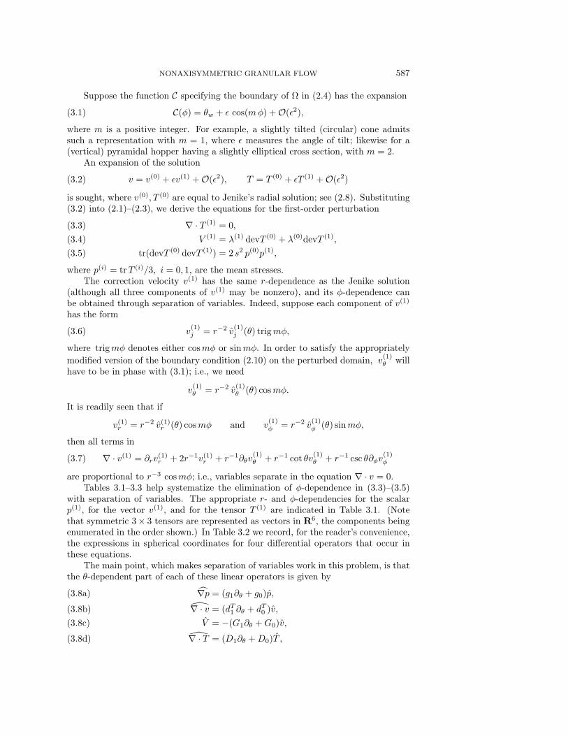
The main point, which makes separation of variables work in this problem, is thatthe θ-dependent part of each of these linear operators is given by

∇p = (g1∂θ + g0)p,(3.8a)

∇ · v = (dT1 ∂θ + dT0 )v,(3.8b)

V = −(G1∂θ +G0)v,(3.8c)

∇ · T = (D1∂θ +D0)T ,(3.8d)


Table 3.1The r- and φ-dependence of scalars, vectors, and tensors in separation of variables.

Scalars : p = r p(θ) cosmφ

Vectors : v = 1r2

[vr(θ) cosmφvθ(θ) cosmφvφ(θ) sinmφ

]Tensors : T = r

Trr(θ) cosmφ

Trθ(θ) cosmφ

Tθθ(θ) cosmφ

Trφ(θ) sinmφ

Tθφ(θ) sinmφ

Tφφ(θ) cosmφ

Table 3.2Differential operators in spherical coordinates.

∇p = [ ∂rp, r−1∂θp, r−1 csc θ∂φp ]T

∇ · v = ∂rvr + 2r−1vr + r−1∂θvθ + r−1 cot θvθ + r−1 csc θ∂φvφ

V =

Vrr

Vrθ

Vθθ

Vrφ

Vθφ

Vφφ

= −

∂rvr

12

(r−1∂θvr − r−1vθ + ∂rvθ

)r−1 (vr + ∂θvθ)

12

(r−1 csc θ ∂φvr − r−1vφ + ∂rvφ

)12r−1(∂θvφ − cot θ vφ + csc θ∂φvθ

)r−1(vr + cot θ vθ + csc θ ∂φvφ

)

∇ · T =

[∂rTrr + r−1 csc θ ∂φTrφ + r−1∂θTrθ + r−1(2Trr − Tφφ − Tθθ + Trθ cot θ)

∂rTrθ + r−1 csc θ ∂φTθφ + r−1∂θTθθ + r−1(3Trθ + (Tθθ − Tφφ) cot θ

)∂rTrφ + r−1 csc θ ∂φTφφ + r−1∂θTθφ + r−1(3Trφ + 2Tθφ cot θ)

]

where g1, g0, . . . , D0 are the matrices given in Table 3.3.The calculation needed to verify (3.8b) was described above; the other equations

may be verified similarly. Incidentally, (3.8a) may be derived by substituting T = pIin (3.8d), and (3.8b) may be derived by taking the trace of (3.8c).

With this notation, (3.3)–(3.5) reduces to a system of ODEs in θ,

(D1∂θ +D0)T(1) = 0,(3.9)

−(G1∂θ +G0)v(1) = λ(1) devT (0) + λ(0)devT (1),(3.10)

tr(devT (0) devT (1)) = 2 s2 p(0)p(1).(3.11)

Recalling the representation of symmetric tensors as 6-component vectors, we observethat the left-hand side of (3.11) may be rewritten as an inner product

tr(devT (0) devT (1)

)= devT (0)TM devT (1),

where M is the 6× 6 matrix

M = diag(1, 2, 1, 2, 2, 1);

thus we may rewrite (3.11) as

devT (0)TMdevT (1) = 2 s2 p(0)p(1).(3.12)


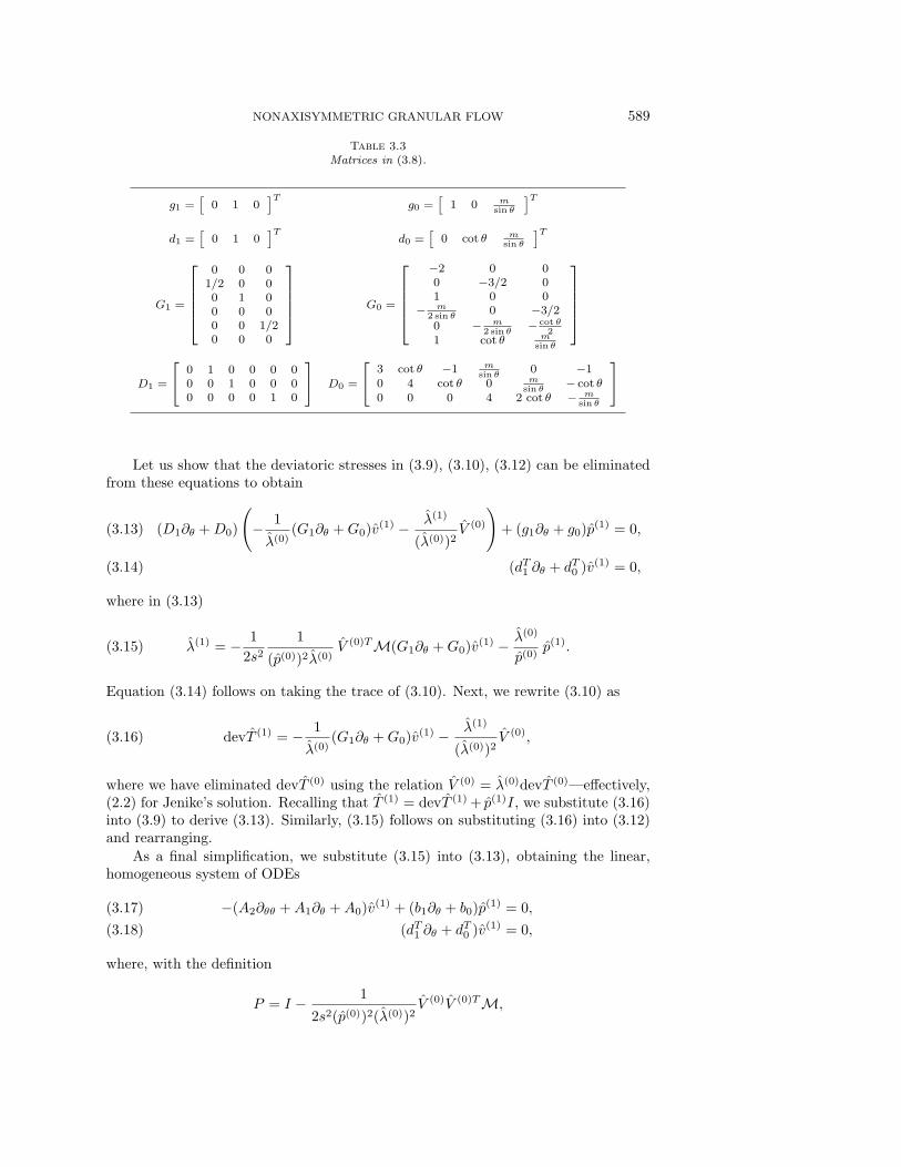
Table 3.3Matrices in (3.8).

g1 =[

0 1 0]T

g0 =[

1 0 msin θ

]Td1 =

[0 1 0

]Td0 =

[0 cot θ m

sin θ

]T

G1 =

0 0 0

1/2 0 00 1 00 0 00 0 1/20 0 0

G0 =

−2 0 00 −3/2 01 0 0

− m2 sin θ

0 −3/2

0 − m2 sin θ

− cot θ2

1 cot θ msin θ

D1 =

[0 1 0 0 0 00 0 1 0 0 00 0 0 0 1 0

]D0 =

[3 cot θ −1 m

sin θ0 −1

0 4 cot θ 0 msin θ

− cot θ0 0 0 4 2 cot θ − m

sin θ

]

Let us show that the deviatoric stresses in (3.9), (3.10), (3.12) can be eliminatedfrom these equations to obtain

(D1∂θ +D0)

(− 1

λ(0)(G1∂θ +G0)v

(1) − λ(1)

(λ(0))2V (0)

)+ (g1∂θ + g0)p

(1) = 0,(3.13)

(dT1 ∂θ + dT0 )v(1) = 0,(3.14)

where in (3.13)

λ(1) = − 1

2s2

1

(p(0))2λ(0)V (0)TM(G1∂θ +G0)v

(1) − λ(0)

p(0)p(1).(3.15)

Equation (3.14) follows on taking the trace of (3.10). Next, we rewrite (3.10) as

devT (1) = − 1

λ(0)(G1∂θ +G0)v

(1) − λ(1)

(λ(0))2V (0),(3.16)

where we have eliminated devT (0) using the relation V (0) = λ(0)devT (0)—effectively,(2.2) for Jenike’s solution. Recalling that T (1) = devT (1) + p(1)I, we substitute (3.16)into (3.9) to derive (3.13). Similarly, (3.15) follows on substituting (3.16) into (3.12)and rearranging.

As a final simplification, we substitute (3.15) into (3.13), obtaining the linear,homogeneous system of ODEs

−(A2∂θθ +A1∂θ +A0)v(1) + (b1∂θ + b0)p

(1) = 0,(3.17)

(dT1 ∂θ + dT0 )v(1) = 0,(3.18)

where, with the definition

P = I − 1

2s2(p(0))2(λ(0))2V (0)V (0)TM,


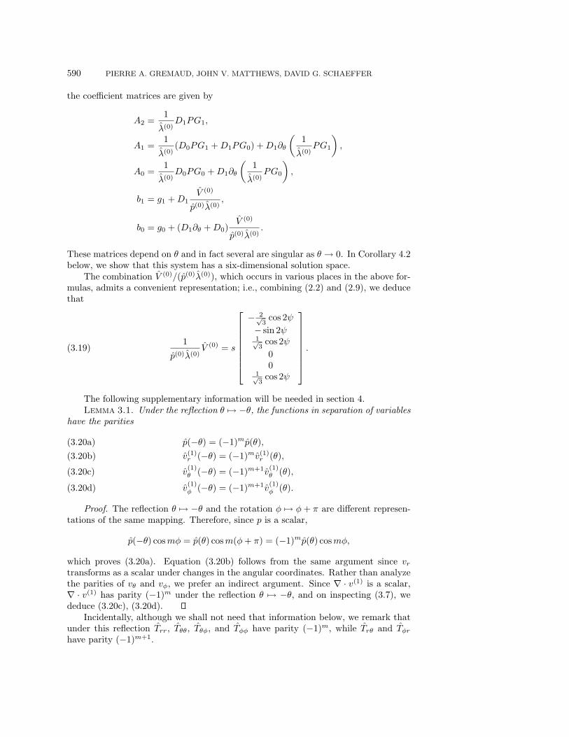
the coefficient matrices are given by

A2 =1

λ(0)D1PG1,

A1 =1

λ(0)(D0PG1 +D1PG0) +D1∂θ

(1

λ(0)PG1

),

A0 =1

λ(0)D0PG0 +D1∂θ

(1

λ(0)PG0

),

b1 = g1 +D1V (0)

p(0)λ(0),

b0 = g0 + (D1∂θ +D0)V (0)

p(0)λ(0).

These matrices depend on θ and in fact several are singular as θ → 0. In Corollary 4.2below, we show that this system has a six-dimensional solution space.

The combination V (0)/(p(0)λ(0)), which occurs in various places in the above for-mulas, admits a convenient representation; i.e., combining (2.2) and (2.9), we deducethat

1

p(0)λ(0)V (0) = s

− 2√3cos 2ψ

− sin 2ψ1√3cos 2ψ

00

1√3cos 2ψ

.(3.19)

The following supplementary information will be needed in section 4.Lemma 3.1. Under the reflection θ → −θ, the functions in separation of variables

have the parities

p(−θ) = (−1)mp(θ),(3.20a)

v(1)r (−θ) = (−1)mv(1)

r (θ),(3.20b)

v(1)θ (−θ) = (−1)m+1v

(1)θ (θ),(3.20c)

v(1)φ (−θ) = (−1)m+1v

(1)φ (θ).(3.20d)

Proof. The reflection θ → −θ and the rotation φ → φ+ π are different represen-tations of the same mapping. Therefore, since p is a scalar,

p(−θ) cosmφ = p(θ) cosm(φ+ π) = (−1)mp(θ) cosmφ,

which proves (3.20a). Equation (3.20b) follows from the same argument since vrtransforms as a scalar under changes in the angular coordinates. Rather than analyzethe parities of vθ and vφ, we prefer an indirect argument. Since ∇ · v(1) is a scalar,∇ · v(1) has parity (−1)m under the reflection θ → −θ, and on inspecting (3.7), wededuce (3.20c), (3.20d).

Incidentally, although we shall not need that information below, we remark thatunder this reflection Trr, Tθθ, Tθφ, and Tφφ have parity (−1)m, while Trθ and Tφr

have parity (−1)m+1.


Table 3.4Leading orders in the expansions at θ = 0 of the coefficient matrices of (3.17)–(3.18).

A2(θ) =

[12

0 0

0 56

0

0 0 12

]+O(θ)

A1(θ) = θ−1

[12

0 0

0 56

m3

0 −m3

12

]+O(1)

A0(θ) = θ−2

−m2

20 0

0 −m2

2− 5

6− 4m

3

0 − 4m3

− 5m2

6− 1

2

+O(θ−1)

b1(θ) = (1 + s/√3)[

0 1 0]T

+O(θ)

b0(θ) = θ−1(1 + s/√3)[

0 0 −m]T

+O(1)

d1(θ) =[

0 1 0]T

(exactly)

d0(θ) = θ−1[

0 1 m]T

+O(1)

3.2. Boundary conditions at the centerline. Equations (3.17), (3.18) havea regular singular point at θ = 0. The leading orders of the coefficient matrices inthese equations are given in Table 3.4. This information may be determined withoutknowing the Jenike solution explicitly since, using the fact that ψ(0) = 0, we deducefrom (3.19) that

V (0)

p(0)λ(0)(0) =

s√3

[ −2 0 1 0 0 1]T

.

According to the method of Frobenius [3], equations (3.17), (3.18) admit solutionsof the form

v(1)(θ) = θνF (θ), p(1)(θ) = θν−1f(θ),(3.21)

where F (θ) and f(θ) are analytic near θ = 0. Suppose the exponent ν is real; if 1 ≤ ν,such a solution is continuous; if ν < 0, it is singular; and if 0 ≤ ν < 1, it is continuous,provided f(0) = 0.

Proposition 3.2. There are exactly three linearly independent solutions of(3.17), (3.18) of the form (3.21) that are continuous at θ = 0.

Proof. Substitution of (3.21) into (3.17), (3.18) gives an indicial equation withroots

ν = ±(m+ 1),±m,±(m− 1).(3.22)

If m ≥ 2, three of the roots of (3.22) are negative and three are positive. The threesolutions associated with the positive indices are linearly independent and continuous.(We remark that since the positive roots differ by integers, in principle these solutions


might contain log terms. This would not affect their continuity. Moreover, usingMaple we have verified that no such log terms arise. See section 5.2 for more detailsabout the Maple code.)

If m = 1, there are four nonnegative roots of (3.22), including zero which is adouble root. Because of a log term, the double root zero contributes at most onecontinuous solution. Again using Maple we have eliminated the various alternativepossibilities to show that zero and the two positive roots (3.22) contribute exactlythree linearly independent continuous solutions and these do not contain any logterms.

Incidentally, since the roots of the indicial equation are integers and since no logterms arise, the continuous solutions of the lemma are actually analytic near θ = 0.

Note that there are six roots (3.22) of the indicial equation. Therefore (3.17),(3.18) has a six-dimensional solution space. (We also prove this by a different ar-gument in Corollary 4.2.) Thus, according to the proposition, the condition thatsolutions be regular at θ = 0 is equivalent to three boundary conditions. Therefore,regularity at θ = 0 plus the three boundary conditions (2.5), (2.6) will provide acomplete set of boundary conditions.

3.3. Boundary conditions at the hopper wall. We derive the perturbedversion of (2.5) in some detail; similar issues arise for (2.6), and we treat the latterequation more succinctly. The calculations are greatly simplified by the fact that wemay neglect any quantity that is O(ε2). To exploit this simplification efficiently, wetemporarily use the notation F ∼ G to mean that F = G+O(ε2).

Including a prefactor of r2 to remove all r-dependence from the equation, we mayrewrite (2.5) as

r2v(r, θw + ε cosmφ, φ) ·N = 0.(3.23)

Because of the perturbation, (3.23) differs from (2.10) in three respects:– the velocity v contains an additional term, v ∼ v(0) + εv(1);– the velocity is evaluated at a location shifted by ε cosmφ;– the direction of the normal N is changed.

Regarding the first two points, we observe that

r2v(r, θw + ε cosmφ, φ) ∼ v(0)(θw) + ε cosmφ∂θv(0)(θw) + ε trigmφ v(1)(θw),

where trigmφ equals cosmφ or sinmφ, depending on the component of v(1). Regard-ing the third point, ∂Ω is the zero set of the function θ − θw − ε cosmφ. Taking thegradient of this function, we conclude that the (inward) normal is

N ∼[0 −1 −ε sinmφ

sin θw

]T.

Modulo an O(ε2)-error, N has unit length. Substituting the previous two equationsinto (3.23), we deduce that

−r2v(r, θw + ε cosmφ, φ) ·N ∼ v(0)θ (θw) + ε cosmφ

(∂θv

(0)θ (θw) + v

(1)θ (θw)

)+ ε

sinmφ

sin θwv(0)φ (θw).

However, since v(0)θ and v

(0)φ vanish identically for Jenike’s solution, the velocity bound-

ary condition for the perturbed problem reduces to

v(1)θ (θw) = 0.(3.24)


We turn to the stress boundary condition (2.6). As regards the scalar τN in (2.6),

we observe that, since T(0)rφ and T

(0)θφ vanish for Jenike’s solution,

τN =

3∑i,j=1

TijNiNj ∼ T(0)θθ + εT

(1)θθ .(3.25)

The vectors τT and vT in (2.6) lie in a two-dimensional subspace tangent to ∂Ω. Notethat the unperturbed tangent space is spanned by the r and φ coordinate directions.Even allowing for the perturbation, the two sides of (2.6) will be equal iff their r- andφ-components are equal; in symbols, iff[

τTr

τTφ

]= −µwτN

|v|[

vrvφ

].

This equality will hold iff (i) the two sides of the equation are parallel vectors and(ii) the first components of the two sides are equal; again, in symbols, iff

τTrvφ − τTφvr = 0 and(3.26)

τTr + µwτN (vr/|v|) = 0.(3.27)

Regarding v, it is clear that[vrvφ

]∼[

v(0)r

0

]+ ε

[v(1)r

v(1)φ

].(3.28)

Regarding τT = τ − τNN , we claim that[τTr

τTφ

]∼ −

[T

(0)rθ

0

]− ε

[T

(1)rθ

T(1)θφ

].(3.29)

Verifying this claim is straightforward except that, in analyzing the second component,

one must invoke the fact that Jenike’s solution satisfies T(0)θθ = T

(0)φφ . On substituting

(3.28) and (3.29) into (3.26), we obtain the equation

ε(T

(0)rθ v

(1)φ − v(0)

r T(1)θφ

)= 0 at θ = θw + ε cosmφ.

The difference between evaluating this expression at θ = θw and at the perturbed lo-cation is O(ε2). Removing the r-dependence (proportional to r) and the φ-dependence(proportional to sinmφ) from this equation, we obtain the first stress boundary con-dition for the perturbed problem:(

T(0)rθ v

(1)φ − v(0)

r T(1)θφ

)= 0 at θ = θw.(3.30)

Regarding (3.27), we claim that

|v| =√

v2r + v2

θ + v2φ ∼ |vr|.

Indeed, it is clear from (3.28) that the contribution of vφ to |v| is O(ε2), and by (3.24)the contribution of vθ to |v| is O(ε4). Thus, vr/|v| ∼ −1. Substituting (3.25) and(3.29) into (3.27), we obtain the condition

(T(0)rθ + εT

(1)rθ ) + µw(T

(0)θθ + εT

(1)θθ ) ∼ 0 at θ = θw + ε cosmφ.


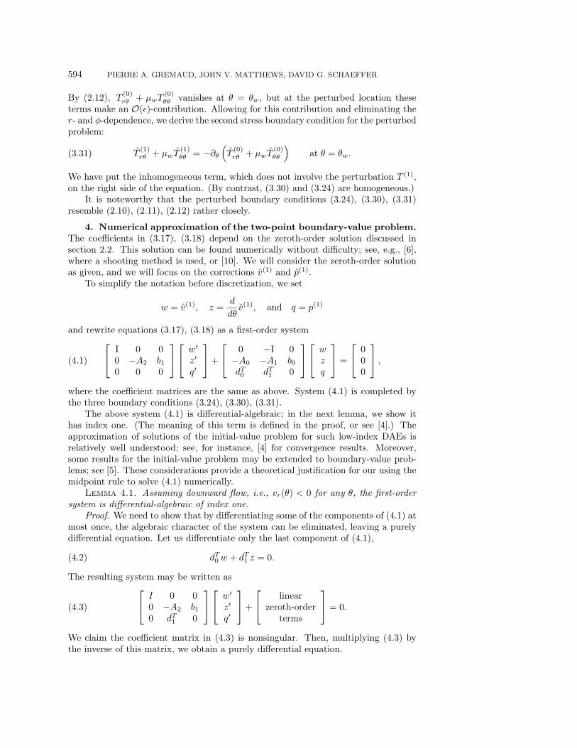
By (2.12), T(0)rθ + µwT

(0)θθ vanishes at θ = θw, but at the perturbed location these

terms make an O(ε)-contribution. Allowing for this contribution and eliminating ther- and φ-dependence, we derive the second stress boundary condition for the perturbedproblem:

T(1)rθ + µwT

(1)θθ = −∂θ

(T

(0)rθ + µwT

(0)θθ

)at θ = θw.(3.31)

We have put the inhomogeneous term, which does not involve the perturbation T (1),on the right side of the equation. (By contrast, (3.30) and (3.24) are homogeneous.)

It is noteworthy that the perturbed boundary conditions (3.24), (3.30), (3.31)resemble (2.10), (2.11), (2.12) rather closely.

4. Numerical approximation of the two-point boundary-value problem.The coefficients in (3.17), (3.18) depend on the zeroth-order solution discussed insection 2.2. This solution can be found numerically without difficulty; see, e.g., [6],where a shooting method is used, or [10]. We will consider the zeroth-order solutionas given, and we will focus on the corrections v(1) and p(1).

To simplify the notation before discretization, we set

w = v(1), z =d

dθv(1), and q = p(1)

and rewrite equations (3.17), (3.18) as a first-order system I 0 00 −A2 b10 0 0

w′

z′

q′

+

0 −I 0−A0 −A1 b0dT0 dT1 0

wzq

=

000

,(4.1)

where the coefficient matrices are the same as above. System (4.1) is completed bythe three boundary conditions (3.24), (3.30), (3.31).

The above system (4.1) is differential-algebraic; in the next lemma, we show ithas index one. (The meaning of this term is defined in the proof, or see [4].) Theapproximation of solutions of the initial-value problem for such low-index DAEs isrelatively well understood; see, for instance, [4] for convergence results. Moreover,some results for the initial-value problem may be extended to boundary-value prob-lems; see [5]. These considerations provide a theoretical justification for our using themidpoint rule to solve (4.1) numerically.

Lemma 4.1. Assuming downward flow, i.e., vr(θ) < 0 for any θ, the first-ordersystem is differential-algebraic of index one.

Proof. We need to show that by differentiating some of the components of (4.1) atmost once, the algebraic character of the system can be eliminated, leaving a purelydifferential equation. Let us differentiate only the last component of (4.1),

dT0 w + dT1 z = 0.(4.2)

The resulting system may be written as I 0 00 −A2 b10 dT1 0

w′

z′

q′

+

linearzeroth-order

terms

= 0.(4.3)

We claim the coefficient matrix in (4.3) is nonsingular. Then, multiplying (4.3) bythe inverse of this matrix, we obtain a purely differential equation.


To prove the claim, it suffices to show that

B =

[+λ(0)A2 b1

dT1 0

](4.4)

is nonsingular, where, without changing invertibility, we have inserted a factor of−λ(0)

in the upper left, which simplifies the calculation. Let us introduce the notation Wfor the column vector on the right-hand side of (3.19), so that V (0)/(p(0)λ(0)) = sW .Then from the definitions following (3.17), (3.18), we have b1 = g1+sD1W. Similarly,

regarding A2, since MG1 = DT1 , we have λ(0)A2 = D1G1 − 1

2 (D1W )(D1W )T . But

D1W =[− sin 2ψ 1√

3cos 2ψ 0

]T.

Hence matrix (4.4) equals

B =

12 − 1

2 sin2 2ψ ∗ ∗ −s sin 2ψ

12√

3cos 2ψ sin 2ψ ∗ ∗ 1 + s√

3cos 2ψ

0 0 12 0

0 1 0 0

,

where ∗ indicates elements that do not affect the invertibility of B. It is readilycalculated that

detB = −1

4

(cos2 2ψ +

s√3cos 2ψ

).

As shown on p. 43 of [12], the assumption that v(0)r < 0 implies that |ψ(θ)| < π/4,

and the claim follows.

Corollary 4.2. The solution space of (4.1) has dimension six.

Proof. The solution space of (4.3), which is seven-dimensional, may be param-

eterized by initial values[

w(θ0) z(θ0) q(θ0)]T

. Since (4.3) was obtained from(4.1) by differentiating (4.2), we conclude that for a solution of (4.3),

dT0 w(θ) + dT1 z(θ) ≡ 0 iff dT0 w(θ0) + dT1 z(θ0) = 0.

Thus the solution space of (4.1) may be identified with the set of solutions of (4.3)whose initial conditions satisfy the scalar equation (4.2).

The boundary-value problem (4.1), (3.24), (3.30), (3.31) is discretized using asymmetric implicit Runge–Kutta method [2], [4]. Since the solutions are expectedto behave smoothly with respect to θ, the simplest of those methods, namely themidpoint rule, is chosen. In spite of being only second-order accurate, this choice isshown to be adequate below. The interval (0, θw) is divided into N subintervals ofsize ∆θ = θw/N , defining a uniform mesh with nodes θi = i∆θ, i = 0, 1, . . . , N . Ateach grid point θi there are seven unknowns,

U i = [wi1 wi

2 wi3 zi1 zi2 zi3 qi]T .

Since there are N+1 grid points, there are 7(N+1) unknowns in total. The midpoint


Table 4.1Numerical boundary conditions at θ = 0.

m = 1 w01 = 0 w0

2 + w03 = 0 z03 = 0 q0 = 0

m ≥ 2 w01 = 0 w0

2 = 0 w03 = 0 q0 = 0

rule for the ODE (4.1) is applied on each interval [θi−1, θi], i = 1, . . . , N , leading to7N equations for the 7(N + 1) unknowns.

Seven additional equations are needed to close the system, and these are providedby the boundary conditions. At θ = θw, the three conditions (3.24), (3.30), (3.31) areimposed, and at θ = 0, the four numerical boundary conditions listed in Table 4.1 areimposed. The latter boundary conditions may be justified as follows. According to(3.21), (3.22), as θ → 0,

w ∼ θν , q ∼ θν−1,

where ν ≥ m− 1. Thus w(0) = 0 if m ≥ 2, and q(0) = 0 if m ≥ 3. In fact, if m = 2,direct calculation of the Frobenius solution (3.21) shows that q(0) = 0 remains truein this case, too. If m = 1, we refer to Lemma 3.1: by parity, w1, q, and z3 = dw3/dθall vanish at θ = 0. The fourth boundary condition in Table 4.1 follows from the lastequation in (4.1) in the limit θ → 0.

The resulting 7(N + 1)× 7(N + 1) system has the following structure:S1 R1

S2 R2

. . .. . .

SN RN

B0 Bw

U0

U1

...

UN−1

UN

=

0

0...

0

Q

.(4.5)

The last row of the above system corresponds to the implementation of the boundaryconditions; the 7 × 7 matrices B0 and Bw contain the coefficients entering in theformula from Table 4.1 and (3.24), (3.30), (3.31), respectively, while Q correspondsto the nonhomogeneous part of the boundary condition (3.31).

5. Numerical results.

5.1. Secondary circulation. We claim that, for solutions of (4.1), secondarycirculation—i.e., flow tangential to the spherical cap r = const—may be describedin terms of the stream function

Ψ =1

mrsin θ sinmφw2(θ).

In other words, we must show that

v(1)θ =

1

r sin θ∂φΨ,(5.1a)

v(1)φ = −1

r∂θΨ.(5.1b)

Since v(1)θ = r−2w2(θ) cosmφ, equation (5.1a) follows by direct differentiation. On


−0.5 −0.4 −0.3 −0.2 −0.1 0 0.1 0.2 0.3 0.4 0.50

0.1

0.2

0.3

0.4

0.5

x

y

−2.2

−2

−1.8

−1.6

−1.4

−1.2

−1

−0.8

−0.6

−0.4

x 10−3

Fig. 5.1. Stream function showing secondary flow in a tilted hopper (m = 1, θw = 30,δ = 30, angle of wall friction = 14), i.e., µw = tan 14. By symmetry, only half of the hopper isrepresented.

−0.5 −0.4 −0.3 −0.2 −0.1 0 0.1 0.2 0.3 0.4 0.50

0.1

0.2

0.3

0.4

0.5

x

y

−6

−4

−2

0

2

4

x 10−4

Fig. 5.2. Stream function showing secondary flow in an “elliptical” hopper (m = 2, θw = 30,δ = 30, angle of wall friction = 14).

the other hand, since v(1)r = r−2w1(θ) cosmφ, we have (∂r + 2r−1)vr = 0, so by (3.7)

(∂θ + cot θ)w2(θ) cosmφ+ csc θ w3(θ) ∂φ(sinmφ) = 0,

from which (5.1b) follows. Figures 5.1 and 5.2 show plots of the level lines of Ψ, whichequal the projection of the streamlines onto a spherical cap r = const. Figure 5.1corresponds to a tilted hopper (m = 1), while Figure 5.2 corresponds to an “ellip-tical” hopper (m = 2). The grains do not move along radial lines but follow morecomplicated and fully three-dimensional trajectories.

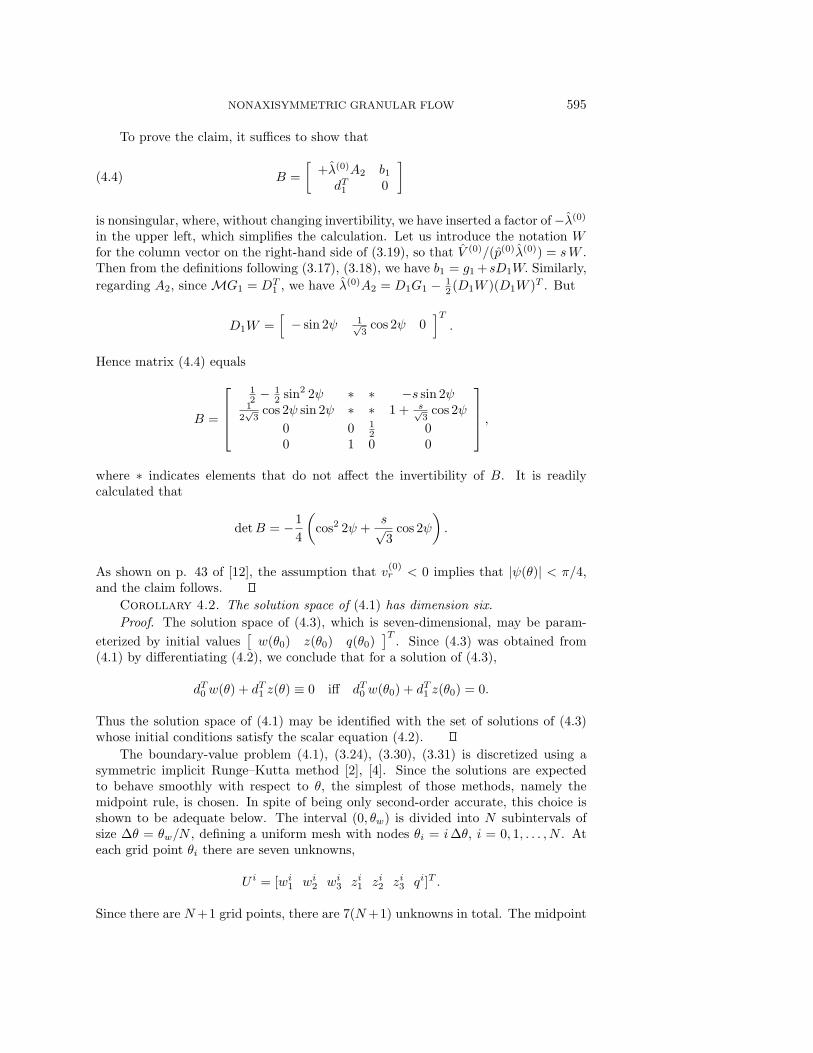
The sign of the main circulation changes when µw increases. The correspondingtransition is independent of the value of m, but is a property of the radial solutionitself. Specifically, the circulation vanishes when the boundary condition for the cor-

rection terms (3.31) is homogeneous, i.e., ∂θT(0)rθ +µw∂θT

(0)θθ = 0 at θ = θw. The range

of θw in Figure 5.3 is limited by the mass-flow limit—exceeding this limit leads toflows with rigid regions, to which the present model does not apply. The range of µw


5 10 15 20 25 30 35 40 45 500

0.05

0.1

0.15

0.2

0.25

0.3

0.35

0.4

0.45

0.5

Half opening angle θw

Wal

l fric

tion

µ w

Fig. 5.3. Critical values leading to sign changes of the circulation (internal friction δ = 30).

−0.5 −0.4 −0.3 −0.2 −0.1 0 0.1 0.2 0.3 0.4 0.50

0.1

0.2

0.3

0.4

0.5

x

y

−0.25

−0.2

−0.15

−0.1

−0.05

0

0.05

0.1

0.15

0.2

−0.5 −0.4 −0.3 −0.2 −0.1 0 0.1 0.2 0.3 0.4 0.50

0.1

0.2

0.3

0.4

0.5

x

y

−0.1

−0.05

0

0.05

0.1

−0.5 −0.4 −0.3 −0.2 −0.1 0 0.1 0.2 0.3 0.4 0.50

0.1

0.2

0.3

0.4

0.5

x

y

−0.08

−0.06

−0.04

−0.02

0

0.02

0.04

0.06

−0.5 −0.4 −0.3 −0.2 −0.1 0 0.1 0.2 0.3 0.4 0.50

0.1

0.2

0.3

0.4

0.5

x

y

−0.06

−0.04

−0.02

0

0.02

0.04

0.06

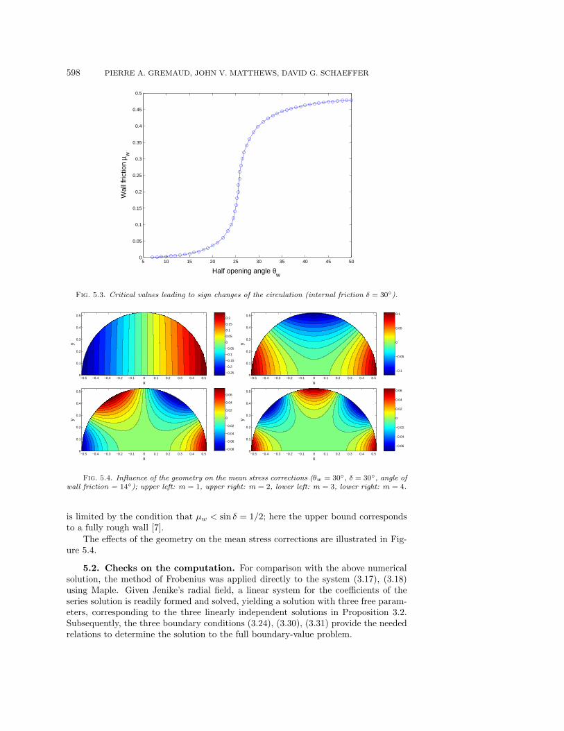
Fig. 5.4. Influence of the geometry on the mean stress corrections (θw = 30, δ = 30, angle ofwall friction = 14); upper left: m = 1, upper right: m = 2, lower left: m = 3, lower right: m = 4.

is limited by the condition that µw < sin δ = 1/2; here the upper bound correspondsto a fully rough wall [7].

The effects of the geometry on the mean stress corrections are illustrated in Fig-ure 5.4.

5.2. Checks on the computation. For comparison with the above numericalsolution, the method of Frobenius was applied directly to the system (3.17), (3.18)using Maple. Given Jenike’s radial field, a linear system for the coefficients of theseries solution is readily formed and solved, yielding a solution with three free param-eters, corresponding to the three linearly independent solutions in Proposition 3.2.Subsequently, the three boundary conditions (3.24), (3.30), (3.31) provide the neededrelations to determine the solution to the full boundary-value problem.


0 0.02 0.04 0.06 0.08 0.1 0.12 0.14 0.16 0.180

0.5

1

1.5

2

2.5

3

3.5

4

4.5

5x 10

−3

θ

v θ(1)

Frobenius Midpoint rule

0 0.02 0.04 0.06 0.08 0.1 0.12 0.14 0.16 0.183

4

5

6

7

8

9

10x 10

−3

θ

Rel

ativ

e di

ffere

nce

(in p

erce

nt)

Fig. 5.5. Comparison of v(1)θ

from the purely numerical method of section 4 and from theFrobenius method of section 5.2. (Using m = 1, θw = 10, δ = 30, and µw = 0.3.)

Two methods of obtaining the radial field were employed. Under the assumptionthat θ2

w and µw/θw are both small and of the same order, a series representation of theJenike field was computed within Maple itself. Under the less restrictive assumptionthat only θw be small (say 10), numerical solutions were computed in MATLAB,fitted to polynomials, and then imported into Maple. In both cases, the resultingpolynomials were then used to compute the first-order correction. The correctionsto the stress and velocity obtained through this symbolic approach agree extremelywell with the results of the purely numerical method of sections 4 and 5: for therepresentative values m = 1, θw = 10, δ = 30, and µw = 0.3, the correctionsobtained by the two different methods have a relative difference of less than 1%; seeFigure 5.5.

Acknowledgments. The authors thank Bob Behringer, Steve Campbell, TimKelley, Tony Royal, and Michael Shearer for many helpful discussions.

REFERENCES

[1] S. Agmon, A. Douglis, and L. Nirenberg, Estimates near the boundary for solutions ofelliptic partial differential equations satisfying general boundary conditions II, Comm. PureAppl. Math., 17 (1964), pp. 35–92.

[2] U.M. Ascher and L.R. Petzold, Computer Methods for Ordinary Differential Equations andDifferential-Algebraic Equations, SIAM, Philadelphia, 1998.

[3] C.M. Bender and S.A. Orszag, Advanced Mathematical Methods for Scientists and Engi-neers, International Series in Pure and Applied Mathematics, McGraw–Hill, New York,1978.

[4] K.E. Brenan, S.L. Campbell, and L.R. Petzold, Numerical Solution of Initial-Value Prob-lems in Differential-Algebraic Equations, Classics Appl. Math. 14, SIAM, Philadelphia,1996.

[5] K.D. Clark and L.R. Petzold, Numerical solution of boundary value problems in differential-algebraic systems, SIAM J. Sci. Statist. Comput., 10 (1989), pp. 915–936.

[6] P.A. Gremaud, J.V. Matthews, and M. Shearer, Similarity solutions for granular materialsin hoppers, in Nonlinear PDE’s, Dynamics, and Continuum Physics, Contemp. Math., 255,J. Bona, K. Saxton and R. Saxton, eds., AMS, Providence, RI, 2000, pp. 79–95.

[7] A.W. Jenike, Gravity flow of bulk solids, Bulletin 108, Utah Eng. Expt. Station, University ofUtah, Salt Lake City, 1961.

[8] T.M. Knowlton, J.W. Carson, G.E. Klinzing, and W.C. Yang, The importance of storage,transfer and collection, Chem. Eng. Prog., 90 (1994), pp. 44–54.

[9] E.W. Merrow, A quantitative assessment of R&D requirements for solids processing technol-ogy, Publication R-3216-DOE/PSSP, Rand Corporation, Santa Monica, CA, 1986.


[10] R.M. Nedderman, Static and Kinematic of Granular Materials, Cambridge University Press,Cambridge, UK, 1992.

[11] N. Rege, Computational Modeling of Granular Materials, Ph.D. thesis, Department of Civiland Environmental Engineering, Massachusetts Institute of Technology, Cambridge, MA,1996.

[12] D.G. Schaeffer, Instability in the evolution equations describing incompressible granular flow,J. Differential Equations, 66 (1987), pp. 19–50.

[13] J.R. Williams and N. Rege, The development of circulation cell structures in granular ma-terials undergoing compression, Powder Technol., 90 (1997), pp. 187–194.

secondarycirculationingranularflowthrough...

Documents