second order differential equation of motion in … between the axles and the bogie’s frame and...

Second Order Differential Equation of Motion in Railways: theVariance of the Dynamic Component of Actions due to the Sprung

Masses of the Vehicles

KONSTANTINOS GIANNAKOSCivil Engineer, PhD, Fellow ASCE, Member TRB AR 050 & 060 Committees

Consultant, Researcher108 Neoreion str., Piraeus 18534

GREECEe-mail addresses: [email protected]; [email protected];

website: http://giannakoskonstantinos.com/wp

Abstract: - In this paper the second order differential equation of motion is presented for the case of a railwayvehicle rolling on a railway track with defects/faults and its solution is presented for the Sprung (Suspended)Masses of the vehicle that act indirectly on the track through the springs and dampers of the vehicle.

Key-Words: - Static/Dynamic Stiffness Coefficient, Sprung Masses, Unprung Masses, Fourier Transform,Spectral Density, Variance, Standard Deviation, Dynamic Component of Actions.

1 IntroductionThe motion of a railway vehicle on the rail runningtable/surface or the motion of a road vehicle on theroad, the response of the structures to earthquakes,etc, is a forced oscillation with a forcing excitation(force), and damping expressed by a random, non-periodic function. The motion is described byequations and, in railway engineering, it isillustrated through the simplified form of a spring-mass-damper system as depicted in Fig. 1, with arailway vehicle running on a track with longitudinaldefects (Fig. 1 left) and the forces exerted on thevehicle’s “car-body” (Fig. 1 right).

Fig. 1 A spring-mass-damper-system in railwayengineering: (left) a railway vehicle on a railwaytrack with longitudinal defects and (right) the forcesexerted on the “car-body”.

In this simplified model, with the wheel rollingover a surface with defects but undeflected itself,the acting forces are:

a. the weight of the vehicle m∙g; b. the dynamic component of the Load Pdyn;c. the motive force P(t) which is equal to the

difference between the tractive force of thelocomotive minus the friction and it ispositive in the case of increase of speed(accelerated motion) or negative in the caseof braking (decrease of speed) since it isequal to zero if the motive force is equal tofriction;

d. the reaction R1 provided by the system“vehicle-track” equal to a spring constant orcoefficient of elasticity ρi (given in kN/mm)multiplied by the subsidence u(x) of thecenter of gravity of the vehicle;

e. the reaction R2 provided by the system“vehicle-track” equal to a damping constantci multiplied by the first derivative of thesubsidence u(x) of the center of gravity ofthe vehicle.

In practice, the circulation of a railway vehicleon a railway track differs significantly from thissimplified model, since the support/railway track isnot undeflected and the railway vehicle has theSprung and the Unsprung Masses as describedbelow. The behavior of the Unsprung Masses (themasses located under the primary suspension of thevehicle) is approached with the track simulated–with the observer situated on the wheel– as anelastic mean with damping as illustrated in the

K. GiannakosInternational Journal of Theoretical and Applied Mechanics

http://www.iaras.org/iaras/journals/ijtam

ISSN: 2367-8992 30 Volume 1, 2016

mailto:[email protected]

mailto:[email protected]

http://giannakoskonstantinos.com/wp

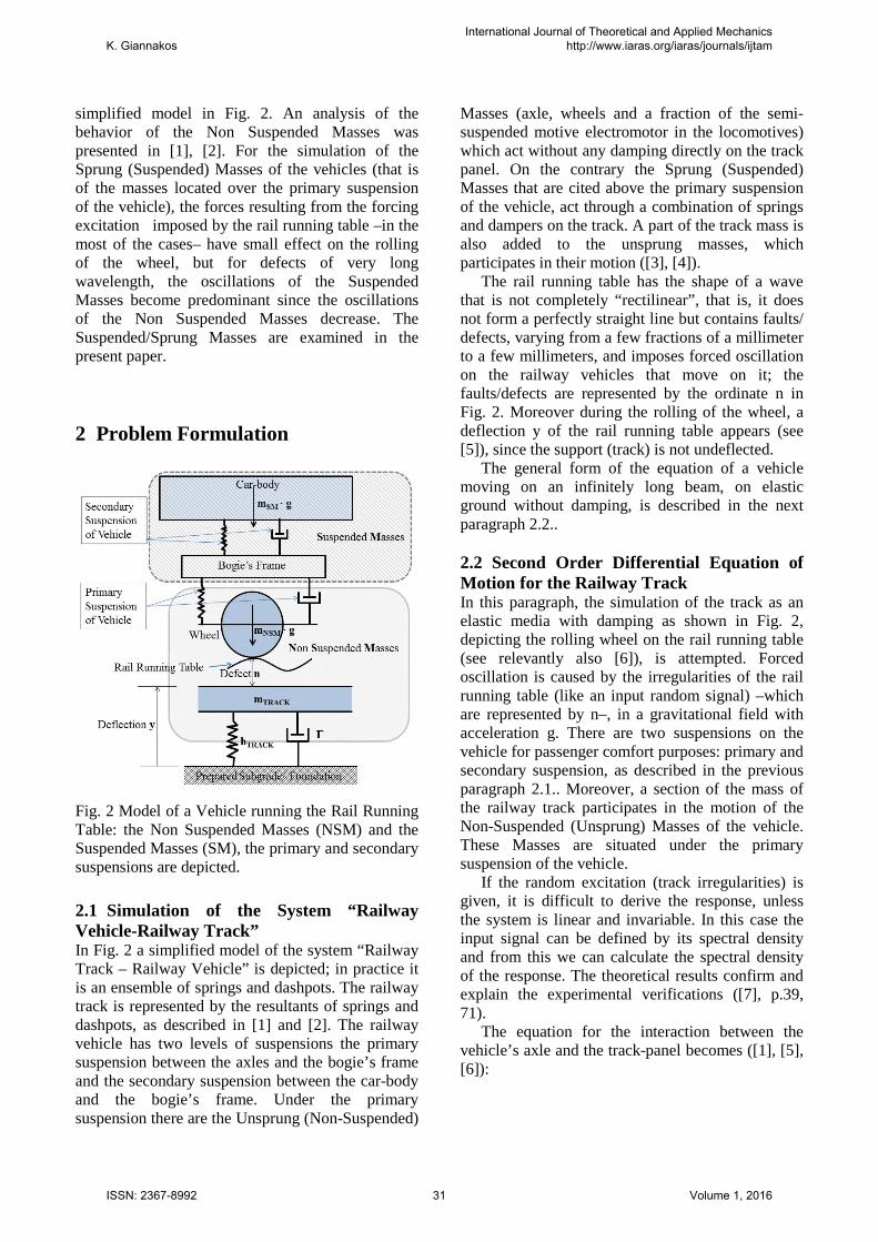
simplified model in Fig. 2. An analysis of thebehavior of the Non Suspended Masses waspresented in [1], [2]. For the simulation of theSprung (Suspended) Masses of the vehicles (that isof the masses located over the primary suspensionof the vehicle), the forces resulting from the forcingexcitation imposed by the rail running table –in themost of the cases– have small effect on the rollingof the wheel, but for defects of very longwavelength, the oscillations of the SuspendedMasses become predominant since the oscillationsof the Non Suspended Masses decrease. TheSuspended/Sprung Masses are examined in thepresent paper.

2 Problem Formulation

Fig. 2 Model of a Vehicle running the Rail RunningTable: the Non Suspended Masses (NSM) and theSuspended Masses (SM), the primary and secondarysuspensions are depicted.

2.1 Simulation of the System “RailwayVehicle-Railway Track”In Fig. 2 a simplified model of the system “RailwayTrack – Railway Vehicle” is depicted; in practice itis an ensemble of springs and dashpots. The railwaytrack is represented by the resultants of springs anddashpots, as described in [1] and [2]. The railwayvehicle has two levels of suspensions the primarysuspension between the axles and the bogie’s frameand the secondary suspension between the car-bodyand the bogie’s frame. Under the primarysuspension there are the Unsprung (Non-Suspended)

Masses (axle, wheels and a fraction of the semi-suspended motive electromotor in the locomotives)which act without any damping directly on the trackpanel. On the contrary the Sprung (Suspended)Masses that are cited above the primary suspensionof the vehicle, act through a combination of springsand dampers on the track. A part of the track mass isalso added to the unsprung masses, whichparticipates in their motion ([3], [4]).

The rail running table has the shape of a wavethat is not completely “rectilinear”, that is, it doesnot form a perfectly straight line but contains faults/defects, varying from a few fractions of a millimeterto a few millimeters, and imposes forced oscillationon the railway vehicles that move on it; thefaults/defects are represented by the ordinate n inFig. 2. Moreover during the rolling of the wheel, adeflection y of the rail running table appears (see[5]), since the support (track) is not undeflected.

The general form of the equation of a vehiclemoving on an infinitely long beam, on elasticground without damping, is described in the nextparagraph 2.2..

2.2 Second Order Differential Equation ofMotion for the Railway TrackIn this paragraph, the simulation of the track as anelastic media with damping as shown in Fig. 2,depicting the rolling wheel on the rail running table(see relevantly also [6]), is attempted. Forcedoscillation is caused by the irregularities of the railrunning table (like an input random signal) –whichare represented by n–, in a gravitational field withacceleration g. There are two suspensions on thevehicle for passenger comfort purposes: primary andsecondary suspension, as described in the previousparagraph 2.1.. Moreover, a section of the mass ofthe railway track participates in the motion of theNon-Suspended (Unsprung) Masses of the vehicle.These Masses are situated under the primarysuspension of the vehicle.

If the random excitation (track irregularities) isgiven, it is difficult to derive the response, unlessthe system is linear and invariable. In this case theinput signal can be defined by its spectral densityand from this we can calculate the spectral densityof the response. The theoretical results confirm andexplain the experimental verifications ([7], p.39,71).

The equation for the interaction between thevehicle’s axle and the track-panel becomes ([1], [5],[6]):



ISSN: 2367-8992 31 Volume 1, 2016

(1)

where: mNSM the Non-Suspended/UnsprungMasses (NSM) of the vehicle in tonnes-mass,mTRACK the mass of the track that participates in themotion of the NSM (for its calculation see Ref. [3]and [4]), mSM the Suspended/Sprung Masses (SM)of the vehicle that are cited above the primarysuspension of the vehicle, Γ damping constant of the track, hTRACK the total dynamic stiffness coefficientof the track (its calculation Eqn. 3 below), n thefault ordinate of the rail running table, g theacceleration of gravity and y the total deflection ofthe track. Furthermore:

(2)

where: ρi the static stiffness coefficients of theconstitutive layers of the track, the quasi springconstants of the layers and ρtotal the resultant totalstatic coefficient of the track and htrack the totaldynamic stiffness coefficient of the track given by:

(3)

with E, J the modulus of elasticity and themoment of inertia of the rail (steel) and ℓ the distance among the sleepers.

The phenomena of the wheel-rail contact and ofthe wheel hunting, particularly the equivalentconicity of the wheel and the forces of pseudo-glide,are non-linear. In any case the use of the linearsystem’s approach is valid for speeds lower than theVcritical≈500 km/h. The integration for the non-linear model (wheel-rail contact, wheel-hunting andpseudoglide forces) is performed through the RungeKutta method ([7], p.94-95, 80, [8], p.98, see also[9], p.171, 351).

In Fig. 2 the rail running table depicts alongitudinal fault/ defect of the rail surface. In theabove equation, the oscillation of the axle is dampedafter its passage over the defect. Viscous damping,due to the ballast, enters the above equation underthe condition that it is proportional to the variationof the deflection dy/dt. To simplify theinvestigation, if we ignore the track mass (for itscalculation Ref. [3] and [4]) in relation to the muchlarger Vehicle’s Non Suspended Mass and bearingin mind that y+n is the total subsidence of the wheelduring its motion (since the y and n are added

algebraically), we can approach the problem of therandom excitation, from cosine defect (V<<Vcritical=500 km/h).

2.3 Fourier Transform and the SecondOrder Differential Equation of MotionWe begin from the hypothesis of a cosine formdefect on the rail running table of the form:

(4)

where: η the ordinate of the defect along the track (abscissa x), V the speed of the vehicle, t thetime and λ the wavelength of the defect, so:

(5a)

since the wheel overpasses the wavelength λ of the defect, in:

(5b)

If we set:

its second derivative will be:

where the quantity represents

the subsidence due to the static loads only, and z

random (see [20]) due to the dynamic loads. Eqn (1)

becomes:

(6a)

(6b)

Since, in this case, we are examining thedynamic loads only (derived from the actions of theSuspended and Non Suspended Masses) , in order toapproach their effect, we could narrow the study ofequation (6b), by changing the variable:

( )

( )

2

2

2

2

+ ⋅ + Γ ⋅ + ⋅ =

= − ⋅ + + ⋅

NSM TRACK TRACK

NSM NSM SM

d y dym m h y

dtdt

d nm m m g

dt

1 1 1 1 1 1

ρ ρ ρ ρ ρ ρ= + + + +

total rail pad sleeper ballast subgrade

41

2 2

totalTRACK dyn totalh E J

ρρ −= = ⋅ ⋅ ⋅

⋅

cos cos 2η ω πλ

⋅ = ⋅ = ⋅ ⋅

V ta t a

2 2 2π π πω ω

ω λ= ⇒ = ⇒ =

VtT t t t

T

λλ= ⇒ = ⋅T T V

V

2 2 2

2 2 2= + ⇒ = +

d u d n d zu n z

dt dt dt

+= + ⋅ ⇒ =SM NSM

TRACK

m m dy dzy z g

h dt dt

2 2

2 2+ Γ ⋅ + ⋅ = − ⋅ ⇒NSM TRACK NSM

d z dz d nm h z m

dt dt dt

2 2

2 20

⇒ + + Γ ⋅ + ⋅ =

NSM TRACK

d z d n dzm h z

dt dt dt

2 2

2 2=

d y d z

dt dt

+⋅NSM SM

TRACK

m mg

h



ISSN: 2367-8992 32 Volume 1, 2016

Equation (6) becomes:

(7a)

(7b)

where, u is the trajectory of the wheel over thevertical fault (of ordinate n) in the longitudinalprofile of the rail.

If we apply the Fourier transform to the equation(6a) (see relevantly Ref. [10] for solving secondorder differential equations with the Fouriertransform):

(8a)

(8b)

(8c)

H(ω) is a complex transfer function, calledfrequency response function [10], that makes itpossible to pass from the fault n to the subsidence Z.If we apply the Fourier transform to equation (7a):

(9)

G(ω) is a complex transfer function, thefrequency response function, that makes it possibleto pass from Z to Z+n.

If we name U the Fourier transform of u, N theFourier transform of n, p=2πiν=iω the variable offrequency and ΔQ the Fourier transform of ΔQ and apply the Fourier transform at equation (7b):

(10a)

where:

(10b)

B(ω) is a complex transfer function, thefrequency response function, that makes it possibleto pass from the fault n to the u=n+Z. Practically itis verified also by the equation:

(10c)

passing from n to Z through H(ω) and afterwards from Z to n+Z through G(ω). This is a formula that characterizes the transfer function between the wheeltrajectory and the fault in the longitudinal level andenables, thereafter, the calculation of the transferfunction between the dynamic load and the trackdefect (fault).

The transfer function B(ω) allows us to calculate the effect of a spectrum of sinusoidal faults, like theundulatory wear. If we replace ω/ωn=ρ, where ωn=the circular eigenfrequency (or natural cyclicfrequency) of the oscillation, and:

where ζ is the damping coefficient. Eqn (10b) is transformed:

(10d)

The transfer function C(ω) of the second

derivative of (Z+n) in relation to time:( )2

2

+d Z n

dt,

–that is the acceleration γ–, will be equal to ω∙Β(ω):

(11a)

that is:

(11b)

2

20+ Γ ⋅ + ⋅ = ⇒NSM TRACK

d u dzm h z

dt dt

( )( )

2

20

−⇒ + Γ ⋅ + ⋅ − =NSM TRACK

d u nd um h u n

dt dt

( )( )

( ) ( )

( ) ( )

2

2

( )ω

ω ω ω ω

ω ω

Γ ⋅⋅ + ⋅ + ⋅ =

= − ⋅ ⇒

TRACK

NSM NSM

i hi Z Z Z

m m

i N

( )( )( )

( )( )

2 42

22 2 2

,ω

ωω

ωω

ω ω

=

⋅=

⋅ − + Γ ⋅

NSM

NSM TRACK

ZH

N

mH

m h

( ) ( ) ( ) ( ) ( ) ( )2 0

0ω ω ω ω ω ω⋅ + Γ ⋅ ⋅ + ⋅ ⋅ = ⇒TRACKi U i Z h i Z

( )( )( )

( )2 2 2

2

2 4,

ω ωω ω

ω ω

+Γ ⋅= =

⋅TRACK

NSM

U hG G

Z m

2

2.(7)⇒ +Γ ⋅ + ⋅ = Γ ⋅ + ⋅ ⇒NSM TRACK TRACK

d u du dnEq m h u h n

dt dt dt

( ) ( )2⋅ + Γ ⋅ + ⋅ = Γ ⋅ + ⋅ ⇒NSM TRACK TRACKm p p h U p h N

( )

( )

( )2

ω

ω ωΓ ⋅ +

= ⋅⋅ + Γ ⋅ +

TRACK

NSM TRACK

B

p hU N

m p p h

( )( )

2 2 22

22 2 2

ωω

ω ω

Γ ⋅ +=

⋅ − + Γ ⋅

TRACK

NSM

hB

m h

( ) ( ) ( )

( )

2 2 2

2 2 2

22 2 2

ω ω ω

ω

ω ω

= ⋅ =

+ Γ ⋅=

⋅ − + Γ ⋅

TRACK

NSM TRACK

B H G

h

m h

( ) ( ) ( )

( ) ( )( )

( )

2 2 2

2

C

p U p B p N

U p B N

ω

ω ω ω

ω ω ω

⋅ = ⋅ ⋅ ⇒

⇒ = ⋅

2 2, , 2 ,

π ωω ω ζω β

λ ω

Γ= = = =TRACK

n n

NSM NSM n

h V

m m

( ) ( )( )

2 22 2

22 2 2

1 4

1 4

ζ βω β

β ζ β

+ ⋅= =

− + ⋅nB B

( ) ( ) ( )

( ) ( )

22 2

2

2 2

n

n

n

C B B

C B

ωω ω ω ω ω

ω

ω ω β ω

= ⋅ = ⋅ ⋅ ⇒

⇒ = ⋅ ⋅



ISSN: 2367-8992 33 Volume 1, 2016

The increase of the vertical load on the track dueto the Non Suspended Masses, according to theprinciple force = mass x acceleration, is given by:

(12)

If we apply the Fourier transform to Eqn. (12):

(13a)

(13b)

2.4 Input and Output Power SpectralDensity and VarianceThe excitation (rail irregularities) in reality israndom and neither periodic nor analytically defined,like the eq. (4). It can be defined by itsautocorrelation function in space and its spectraldensity ([7], p.58; [11], p.700; [12]). If f(x) is asignal with determined total energy and F(ν) its Fourier transform, from Parseval’s modulus theorem[13], the total energy is [10]:

(14a)

where, F(ν)=Α(ν)∙eiφ(ν) and the power spectraldensity:

(15)

Reference [10] solves equation (14a) as:

(14b)

The square of the modulus F(ω) is called the energy spectrum of the signal because F2(ω)∙Δ(ω) represents the amount of energy in any ΔΩ segment of the frequency spectrum, and the integral of F2(ω) over (-∞, +∞)gives the total energy of the signal. An input signal -like the running rail table- createsthrough the vehicle an output signal: the wheeltrajectory. The output spectral density and the inputspectral density of the excitation are related throughequation [14], [5]:

(15a)

In order to relate the temporal spectrum with thespectrum in space we use the following equation:

(15b)

where λ is the wavelength of the defect. This means that circular frequency in space Ω is the wave number k of the equation of oscillation, and [13]:

(16a)

whereF is the symbol for the application of theFourier transform of f and f the function after thetransform. This is a property of the Fouriertransform.

Eqn (16a) applied in the case that the powerspectrum of the vertical defects along the track (forthe NSM) in the space domain is S(Ω) then the power spectrum of the excitation of the wheel in thetime domain will result after a replacement of Ω by the ω/V.

(16b)

The Variance or mean square value σ2(x) of thefunction is given by [15], [16]:

( ) ( )2 21

2σ ω ω

π

+∞

−∞

= ⋅ ⋅ =∫x S d x (17)

where σ(x) is the standard deviation of the function.

The Power Spectral density and the variance of afunction are depicted in Fig. 3.

From equation (17) we derive:

( ) ( )

( ) ( )

( ) ( )

2

0

2

0

2

0

1

1

1

σ ω ωπ

σ ω ωπ

σ ω ωπ

+∞

+∞

+∞

∆

= ⋅

= ⋅

∆ = ⋅

∫

∫

∫

n

z

Q

n S d

z S d

Q S d

(18)

where n is the random variable of the defect(input), z the subsidence of the wheel (output) andΔQ the dynamic component of the Load that is added to the Static Load of the wheel due to the NonSuspended Masses (output also).

From these equations and the analytic form ofthe spectrum of the defects/faults, we can calculatethe mean square value of the dynamic component ofthe Load due to the Non Suspended Masses that isadded to the relevant dynamic component of the

( )22

2 2

+∆ = ⋅ = ⋅NSM NSM

d n Zd uQ m m

dt dt

( ) ( )2 2 ˆˆ ω ω+∆ = ⋅ ⋅ = ⋅ ⋅ ⇒NSM NSM Z nQ m p U m p f

( ) ( ) ( ) ( )2ˆ

NSM NSMQ m C N m p B Nω ω ω ω∆ = ⋅ ⋅ = ⋅ ⋅ ⋅

( ) ( )2 2

ν ν+∞ +∞

−∞ −∞

⋅ = ⋅∫ ∫f x dx F d

( ) ( ) ( )2 2ω ν ν= =S F A

( ) ( )2

2 1

2ω ω

π

+∞ +∞

−∞ −∞

⋅ = ⋅∫ ∫f t dt F d

( ) ( ) ( )2

OUTPUT INPUTS H i Sω ω ω= ⋅

2 2π πω ω ω

λ λ⋅ = ⇒ = ⋅ ⇒ =Ω⋅

Vtt V V

( ) ( )0 0

ω ω∞ ∞

Ω ⋅ Ω = ⋅ ⇒∫ ∫S d s d

( )1

s SV V

υ

ωω

=

( )

( ) ( )

1 ˆ

1

f ax fa a

S S SV V

ν

ωω

⇒ = ⋅ ⇒

⇒ = = ⋅ Ω

F

( ) ( )2 2ˆNSM nQ m B Nβ ω ω ω∆ = ⋅ ⋅ ⋅ ⋅



ISSN: 2367-8992 34 Volume 1, 2016

Suspended Masses and the total dynamic componentof the load is added to the Static Load of the wheel.

Fig. 3 Power Spectral density S(Ω) –the black curve– Variance (mean square value x2) –the shadedarea– of a function [5].

From the power spectral density and the variancefunctions and their definitions [5]:

(19a)

(19b)

(19c)

and using the eqs. (19) and (11-12b):

(20)

(21)

From the above equations and the analytical formof the spectrum of the longitudinal defects/ faults ofthe track we could effectively calculate the variance(mean square value) of the dynamic component ofthe Loads on the track panel due to the NonSuspended Masses. All the results of measurementson track in the French railways network show thatthe spectrum of defects in the longitudinal level hasthe form [6], [17]:

( )( )

3n

AS

BΩ =

+Ω(22)

This implies that the mean square value orvariance of the defects is given by:

(23)

If we examine only the much more severe case,for the case of the Non Suspended Masses, of thedefects of short wavelength, consequently large Ω –like the undulatory wear– then we can omit theterm B, and using Eqn. (15b):

(24)

The term B characterizes the defects with largewavelengths, for which the maintenance of track iseffective, and when we examine this kind of defectsterm B should be taken into account. SuspendedMasses should be examined for long wavelengthdefects.

For the line “Les Aubrais – Vierzon”, theparameters values are: B=0,36, A=2,1∙10-6 and S(Ω) is calculated in m3 and σ(z)=1,57 mm. The eigenfrequency of the Non Suspended Masses of thevehicles is approximately 30 – 40 Hz and even forspeeds of 300 km/h there are wavelengths less than3 m [17].

From equations (16) and (24):

(25)

3 The Case of Non Suspended Masses

This case has been analyzed in [1], [2], [5], [18].The interested reader should read the relevant texts.

4 The Variance of the SuspendedMasses

If we assume that the defects of the two rails–constituting the cross-section of a track– are quitethe same at the same time and presenting the samephase, or if we examine the trajectory of one wheel,

( )3

3 33

3

1 ωω

⋅Ω = = =

Ω ⋅n

A A A VS

V

( ) ( ) ( )2

ω ω ω∆ = ⋅Q nS S B

( ) ( )

( )( )

2 2

2

2

γ σ σ γ

σσ γ

∆ = ⋅∆ ⇒ ∆ = ⋅ ⇒

∆⇒ =

NSM NSM

NSM

Q m Q m

Q

m

( ) ( )

( ) ( ) ( )

2 2

22

2

0

1

1

σ γ σ

σ γ ω ω ωπ

+∞

= ⋅ ∆ ⇒

= ⋅ ⋅ ⋅⋅ ∫

NSM

n

NSM

Qm

B S dm

( ) ( ) ( )2

22 4 4

2

0

σ γ β ω ω ω ωπ

+∞

= ⋅ ⋅ ⋅ ⋅ ⋅ =⋅ ∫

NSMn n

NSM

mB S d

m

( )

( )( )

2

2 24 4

22 2 20

1 1 4

1 4

σ γ

ζ ββ ω ω ω

π β ζ β

+∞

=

+ ⋅= ⋅ ⋅ ⋅ ⋅ ⋅

− + ⋅∫ n nS d

( )( )

2

3

0

1 Az d

Bσ

π

+∞

= ⋅ ⋅ Ω⇒+Ω

∫

( )2

2

1

2σ

π= ⋅

Az

B

( ) ( )3 2

3 3 3

1 1ω

ω ω β

⋅ ⋅= ⋅ Ω = ⋅ =

⋅n

n

A V A VS S

V V

( )

( )

2

2 20

2

2

1

2 2

10

2

σπ

σπ

+∞

= − ⋅ ⇒ + Ω +Ω

⇒ = − − ⇒

Az

B B

Az

B

( )( ) ( )

2

3 2

00

1 1

2

A Az dx

x Bσ

π π

+∞+∞

⇒ = ⋅ ⋅ = − ⇒ +Ω

∫



ISSN: 2367-8992 35 Volume 1, 2016

then the conclusion that will be derived can be usedfor more complicated cases of rolling of vehicles,motion of car-bodies etc. Furthermore we considerthe simplified model of Fig. 1 with one-floor mass-spring-damper system rolling on a rail’s surface.

In order to calculate the power spectrum densityof the excitation sE(ω) from the excitation spectrum of the wheel sυ(ω), we apply the Eqn. 15a with the Eqns. 16, Eqn. 22 (the parameter B is not omitted)and Eqns. 10 (in order to pass from the defect n ton+Z):

(26)

where: sE(ω) is the power spectrum density of the excitation, ωn is always the eigenfrequency of theNon Suspended Masses, ζ the damping coefficient of the track, sυ(ω) the spectrum of the excitation of the wheel due to the track defects/faults andB(ω)the modulus of the transfer function of the motion of the wheel.

From the Eqns. 10 and the Eqns. 11, 12 and 13,

with the analysis cited above, we keep that, C(ω) ις

the transfer function of the second derivative of

(Z+n) in relation to time: , that is the

acceleration γ and it is equal to ω∙B(ω).

In the case of the Suspended Masses C(ω)is the modulus of the transfer function of theaccelerations of the car-body. Consequently for thespectrum of the accelerations of the car-body we willuse Eqn. 15a substituting the parameters ζ and ωn ofthe track with the relevant parameters ζ′ (damping coefficient) and ω′n (eigenfrequency) of the car-body.

For the railway vehicles the eigenfrequencies ω′nof the car-body are in the area of 1 Hz, since with thedevelopment of high-speeds it could arrive 10 Hz.For the damping coefficient of the car-body of therailway vehicles two characteristic values of ζ′ could be used with reliability: 0,15 and 0,20 (see relevantly[17] and [7]).

(27)

The variance of the accelerations of the car-bodyof the railway vehicles is given by (Eqns. 18):

(28)

which converges for ω infinite. Consequently the variance of the part of the dynamic component ofthe load due to the Suspended/Sprung Masses of thevehicle is given by (see Eqn. 19b):

(29)

Finally an approximation could be used for thecalculation of the variance of this part of thedynamic component of the load (see [5], [6]):

(30)

where: Qwheel is the static wheel load, V is theoperational speed, and the coefficient NL is themean standard deviation of the longitudinal levelcondition of the track, on a 300 m lengthapproximately, for both rails is the mean standarddeviation of the longitudinal level condition of thetrack, on a 300 m length fluctuating between 0,7–1,5 mm or more (see [6]; [19], p. 335–336); for theGreek network NL is estimated to fluctuate –mainly– between 1 and 1,5 [5].

In more details NL, the average of the brutalsignal on a basis of approximately 300 m for thevertical and horizontal defects of the two rails, is theconvolution:

(31)

where ηl(x) is the value of the primary signal; in practice a weighted average index which “crashes”less the isolated defects than one classic average andsimulates roughly the “memory” of the vehicle (seerelevantly [19]).

( ) ( ) ( )

( )( )

2

22

2 2

2 32 2

2

2 2

1 4

1 4

E

nE

n n

s B s

AVs

BV

υω ω ω

ωζ

ωω

ωω ωζ

ω ω

= ⋅ ⇒

+ ⋅

⇒ = ⋅+

− + ⋅

( )2

2

d Z n

dt

+

( ) ( ) ( )2

Es C sγ ω ω ω= ⋅ ⇒

( )( ) ( )

( )

2 2 24

3 22 2 2

2 2

22 2 2

1 4

1 4

1 4

1 4

n

AVs

BVγ

ζ βω ω

ω β ζ β

ζ β

β ζ β

+ ⋅= ⋅ ⋅ ⋅

+ − + ⋅

′ ′+ ⋅⋅

′ ′ ′− + ⋅

( ) ( )2

0

1s dγσ γ ω ω

π

∞

= ⋅ ⋅∫

( ) ( )2 2SM SM SM SMQ m Q mγ σ σ γ∆ = ⋅∆ ⇒ ∆ = ⋅

( )40

1000SM L wheel

VQ N Qσ

−∆ = ⋅ ⋅

( ) ( )0

3000

1

300

x x

LN x l x e dxη− +∞

−∞

= ∫



ISSN: 2367-8992 36 Volume 1, 2016

5 Conclusions

In this paper the second order differential equationof motion of the Sprung (Suspended) Masses of arailway vehicle rolling on the track withdefects/faults is investigated and its solution isapproached. The investigation is performed throughthe Fourier transform and the solution is verifiedfrom findings from a research program performedby the Greek railways in collaboration with theFrench state railways (SNCF) and further researchperformed by the author.

References:[1] Giannakos K. Modeling the Influence of Short

Wavelength Defects in a Railway Track on theDynamic Behavior of the Non-SuspendedMasses, Journal of Mechanical Systems andSignal Processing (Mech. Syst. SignalProcess.), Elsevier, 2015, Vol. 68-69, 2016, pp.68-83.

[2] Giannakos K. Track Defects and the DynamicLoads due to Non-Suspended Masses ofRailway Vehicles, NAUN International Journalof Mechanics, Vol.7, Issue 3, 2013, pp. 180-191.

[3] Giannakos K. Theoretical calculation of thetrack-mass in the motion of unsprung masses inrelation to track dynamic stiffness anddamping, International Journal of PavementEngineering (IJPE), Special Rail Issue “High-Speed Railway Infrastructure: RecentDevelopments and Performance”, Vol. 11,Issue 4, August 2010, pp. 319-330.

[4] Giannakos K. Influence of the track's dampingon the track mass participating in the motion ofthe Non Suspended Masses of railway vehicles– theoretical calculation and comparison tomeasurements, volume published in honour of(fs) professor George Giannopoulos, AristotleUniversity of Thessaloniki, 2012.

[5] Giannakos K. Actions on the Railway Track,Papazissis publ., www.papazisi.gr, Athens,2004.

[6] SNCF/Direction de l’ Equipement, Mecaniquede la Voie, 1981.

[7] Alias J. La Voie Ferree – Techniques deConstruction et Entretien, deuxieme edition,Eyrolles, Paris, 1984.

[8] Fortin J. La Deformee Dynamique de la VoieFerree, Revue Generale des Chemins de Fer(RGCF), 02/1982.

[9] Thompson D. Railway Noise and Vibration,Elsevier, 2009.

[10] Wylie C.R. and Barrett L.C. AdvancedEngineering Mathematics, sixth edition,McGraw-Hill, Inc., USA, 1995.

[11] Gent I. and Janin G. La Qualite de la VoieFerree, SNCF’s reprint.

[12] Papoulis A. Signal Analysis, McGraw-Hill Inc.,USA, 1977.

[13] Roddier F. Distributions et Transformation deFourier, Edisciense, Paris, 1971.

[14] Clough R.W. and Penzien J. Dynamics ofStructures, second edition, McGraw-Hill Intl.,Singapore, 1993.

[15] Papoulis A. Probability, Random Variablesand Stochastic Processes, third edition,McGraw-Hill Intl., Singapore, 1991.

[16] Spiegel M.R. Probability and Statistics,Schaum’s Outline Series, McGraw-Hill, NewYork, greek edition, Athens, 1977.

[17] Prud’Homme A. La Voie, Revue Generale desChemins de Fer (RGCF), Janvier, 1970, extraitde RGCF.

[18] Giannakos K. and Loizos A. Evaluation ofactions on concrete sleepers as design loads –Influence of fastenings, International Journalof Pavement Engineering (IJPE), Vol. 11, Issue3, June 2010, pp. 197 – 213.

[19] Janin G. La Maintenance de la Geometrie de laVoie, Revue Generale des Chemins de Fer(RGCF), Juin, 1982, pp. 331–346.



ISSN: 2367-8992 37 Volume 1, 2016

second order differential equation of motion in … between the axles and the bogie’s frame and...

Documents