second interim report: 3. ex-ante assessment of the proposed funding system

Final version – March 12, 2015

R&D Evaluation Methodology and Funding Principles Background Report to the 2nd Interim Report: Ex-ante assessment of the proposed funding system

R&D Evaluation Methodology and Funding Principles

Background report to the 2nd Interim Report: Ex-ante assessment of the proposed funding system

March, 2015

Tomas Ratinger, TC SACR Ondrej Pecha, TC ASCR


R&D Evaluation Methodology and Funding Principles i

Table of Contents 1. Introduction 4

2. The architecture for the ex-ante assessment 7

2.1 Mathematical description of institutional funding 7 2.2 The architecture of the quantitative assessment tool for the assessment of institutional funding proposals 10 2.3 Parameters to be specified 11 2.4 Scenarios 17 2.5 Running simulations 18 2.6 Visualisation of the results 22

3. Results of the simulations 23

3.1 Investigated issues 23 3.2 Scenarios for the distribution of the funding in the PRFS sub-pots 24 3.3 The size effect in the Option 1 approach to PRFS (person-scores) 28 3.4 The Option 2 approach (relative scores) 34

4. Conclusions 37


ii R&D Evaluation Methodology and Funding Principles

Table of Figures Figure 1 The three components of institutional funding .................................................. 5 Figure 2 Basic architecture of the quantitative tool ....................................................... 11 Figure 3 Model scheme ................................................................................................... 14 Figure 4 An example of scenarios .................................................................................. 20 Figure 5 Comparison of the Client and Radical scenarios in respect to the Basic scenario. (Option 1 PRFS, period 1) ............................................................................... 26 Figure 6 Total (average) scores and percentage change of total IF .............................. 28 Figure 7 the relationship between the evaluation scores (Total Score) and PRFS allocations ....................................................................................................................... 29 Figure 8 The relationship between RIV points intensity (RIV points/AR) and the Total Score resulting from the new evaluation methodology. ................................................ 30 Figure 9 The output intensity and IF change. ................................................................ 31 Figure 10 Percentage change of Total IF, quartic transformation ................................ 32 Figure 11 IF distributions in Period 2 and Period 3 relatively to IF allocations in Period 1. ...................................................................................................................................... 34 Figure 12 The relationship between evaluation scores and % change of IF in Option 2 in the first period ............................................................................................................ 35 Figure 13 The changes of IF after three evaluation and funding periods – Option 2 ... 36

List of Tables

Table 1 Criteria for PRFS budget adjustment .................................................................. 8 Table 2 Implementation parameters to be specified ...................................................... 11 Table 3 Alternative distributions of PRFS budget into the sub-pots. ............................ 16 Table 4 Comparison of scenario in respect to the Basic scenario. (Option 1 PRFS) .... 24 Table 5 Comparison of scenario in respect to the Basic scenario. (Option 1 PRFS, period 1) – differentiated by RO types. ......................................................................... 26 Table 6 Comparison of scenario in respect to the Basic scenario. (Option 2 PRFS) ..... 27 Table 7 Comparison of scenario in respect to the Basic scenario. (Option 1 PRFS) – total IF ............................................................................................................................. 27 Table 8 IF changes, number of cases (EvUs) in various categories of significance. ...... 31 Table 9 The benefit of quartic transformation of scores ............................................... 33


4 R&D Evaluation Methodology and Funding Principles

1. Introduction

This background report to the 2nd Interim Report describes the processes and tools as well as the outcomes of the study activities for the design of the new funding principles related to the following objectives: 1. To develop RO models for assessing the impacts of the proposed funding system

across several years.

2. To conduct an impact assessment of the proposed funding schemes

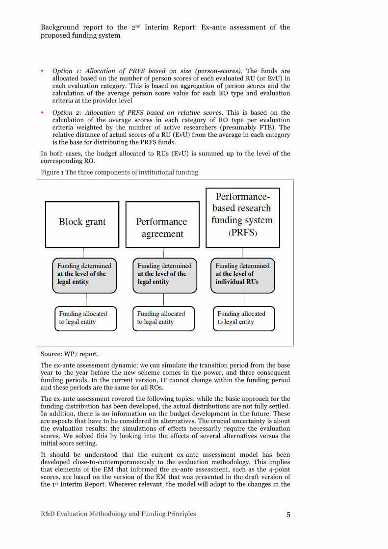
The proposed new institutional funding (IF) system is described in the 2nd Interim Report. As shown in Figure 1, below, it consists of three elements

• Block grant (Block) – fixed sum or proportion of the public funding budget allocated to a research organisation (RO). The research organisation commits itself to reaching some long-term strategic targets for development, when using these resources.

• Performance agreements (PA)

• Performance-based research funding (PRFS) – proportion of the public funding budget that is specifically dedicated for the funding of research and is driven by indicators that assess the performance of the organisations, such as quality of the research, relevance for innovation/society etc.

This distribution is illustrated in the scheme below (Figure 1).

In the 2nd Interim Report it is proposed that the IF budget (of a provider) is first allocated to two IF components (Block, PA) as a fixed proportion of the past (base year) IF. The PRFS part will be adjusted to the actually available budget (i.e. it can decrease, stay the same or increase).

In the next step, the PRFS component is further distributed to pots per RO types (ScRO, IBRO, PSRO and NatRes) and based on the evaluation criteria (Scientific research excellence, Overall research performance, Societal Relevance, Membership of the (global and national) research community and Research Environment1).

In this report and in the simulation model, the following abbreviations for the types of RO are used:

• ScRO - Scientific Research organisations

• IBRO – Industry & Business Research Organisations

• PSRO – Public Service Research Organisations

• NatRes - National resources /Infrastructure Research Organisations

Distribution of the PRFS pots to individual RO (legal entities) will be based on performance against each of the 5 assessment criteria as expressed in the evaluation scores. Two options for translating scores into funding are considered in the 2nd Interim Report:

1 These are abbreviations for the 5 assessment criteria defined in the EM, respectively Research environment, Membership of the global and national research community, Scientific research excellence, research performance, and Societal relevance (see the 1st Interim Report)


R&D Evaluation Methodology and Funding Principles 5

• Option 1: Allocation of PRFS based on size (person-scores). The funds are allocated based on the number of person scores of each evaluated RU (or EvU) in each evaluation category. This is based on aggregation of person scores and the calculation of the average person score value for each RO type and evaluation criteria at the provider level

• Option 2: Allocation of PRFS based on relative scores. This is based on the calculation of the average scores in each category of RO type per evaluation criteria weighted by the number of active researchers (presumably FTE). The relative distance of actual scores of a RU (EvU) from the average in each category is the base for distributing the PRFS funds.

In both cases, the budget allocated to RUs (EvU) is summed up to the level of the corresponding RO.

Figure 1 The three components of institutional funding

Source: WP7 report.

The ex-ante assessment dynamic; we can simulate the transition period from the base year to the year before the new scheme comes in the power, and three consequent funding periods. In the current version, IF cannot change within the funding period and these periods are the same for all ROs.

The ex-ante assessment covered the following topics: while the basic approach for the funding distribution has been developed, the actual distributions are not fully settled. In addition, there is no information on the budget development in the future. These are aspects that have to be considered in alternatives. The crucial uncertainty is about the evaluation results: the simulations of effects necessarily require the evaluation scores. We solved this by looking into the effects of several alternatives versus the initial score setting.

It should be understood that the current ex-ante assessment model has been developed close-to-contemporaneously to the evaluation methodology. This implies that elements of the EM that informed the ex-ante assessment, such as the 4-point scores, are based on the version of the EM that was presented in the draft version of the 1st Interim Report. Wherever relevant, the model will adapt to the changes in the



EM that have been introduced in the final version of the 1st Interim Report (and any eventual other changes in the future).

This report is structured as follows:

• We first describe the technicalities and processes for the ex-ante assessment, i.e. the modelling tool (Section 2)

• In Section 3 we report on the outcomes of the simulations that were performed so far in the context of this study. In the 2nd Interim report we identified different scenarios for the weighting of the evaluation criteria in the PRFS pots per RO type. In this report, we refer to these as PRFS scenarios.



2. The architecture for the ex-ante assessment

2.1 Mathematical description of institutional funding

2.1.1 Introduction Under Institutional funding we understand the general funding of institutions with no direct selection of R&D project or programmes. In the current Czech system it is the support to the development of the research organisation.

In our analysis, we consider also the former ‘research intentions’ funding (vyzkumne zamery) as a form of institutional funding since they were not subject to competition among research organisations or teams and actually have been replaced by the ‘support to the development of research organisations’ budget line.

The institutional financing Y of a RO (j) of the RO-type (i) in time (t) is given by three components

𝑌!"! = 𝐵!"! + 𝑃!"! + 𝑋!"! ,

Where 𝐵!"! stands for the block financing, 𝑃!"! for performance agreement and 𝑋!"! represents the performance based component (PRFS). 𝐵!"! and 𝑃!"! are given as fixed proportions (α and β respectively) of the previous year institutional budget 𝑌!"!!!. In this sense, their modelling is simple.

The budget 𝑋!! for the RO-type (i) will be distributed to individual ROs (j=1,…, ni)

𝑋!! = 𝑋! !,!

!. (1)

There are two main options to do it which will be discussed below. For the both options it holds

i) 𝑋!! is largely predetermined

𝑋!! = (1 − 𝛼 − 𝛽)𝑌!!!!𝑔!, (2)

where gt is an index of the R&D budget growth (it can also be made RO-type specific or provider specific)

ii) 𝑋!! is distributed to five pots according to evaluation criteria (Excellence, Performance, Societal impact, Internationalization, Management),

𝑋!,!! = 𝑤!"𝑋!!, k=1,…,5

where wik are weights of social importance of research conduct aspects (different for each RO-type) for which holds 𝑤!"!

!!! = 1. The weights are exogenous, they should be agreed by R&D policy makers.

2.1.2 Option 1

The idea of Option 1 is that the distribution of the PRFS budget (𝑋!!) to individual ROs (equation 1) is done on the basis of manscores i.e. the number of scientific staff times (𝐿!!!!) the score in the k-th evaluation criterion 𝐸!,!,!! . Thus for each RO (j) the manscore 𝐸!,!,!! = 𝐿!!!!𝐸!,!,!! . The total of manscores for the i-th RO-type and criterion k is given by

𝐸!,!! = 𝐿!!!!𝐸!,!,!!!!!!! ,

Note, that we use the upper index t in the case of the current evaluation and the index t-1 for scientific labour. Concerning the latter, it is because the labour refers to the period before evaluation, based on evaluation and the respective IF allocation it will grow at the half rate of the IF budget change (Lt will be determined by Xt and Yt ).



The PRFS budget (𝑋!,!,!! ) will be allocated to a RO (j) by using the share of j-manscores on the total manscores in the particular evaluation area (k) i.e.

𝑋!,!,!! = 𝑋!,!!!!,!,!!

!!,!! = 𝑋!"!

!!!!!!!,!,!

!

!!!!!!!,!,!

!!!!!!

= 𝑋!!𝑤!,!!!!!!!!,!,!

!

!!!!!!!,!,!

!!!!!!

, (3)

Finally, the PRFS budget of the RO j will be

𝑋!,!! = 𝑋!! 𝑤!,!!!!!!!!,!,!

!

!!!!!!!,!,!

!!!!!!

!!!! = (1 − 𝛼 − 𝛽)𝑌!!!!𝑔! 𝑤!,!

!!!!!!!,!,!

!

!!!!!!!,!,!

!!!!!!

!!!! . (4)

If we have ROs with several evaluated units (EvU) then we do the same algorithm as above and we summarise PRFS values of EvUs to the RO levels.

2.1.3 Option 2 The idea of the Option 1 is that we calculate weighted average score for each of the k evaluation areas/criteria. The financing will reflect the departure of the RO from that average. This departure will increase or decrease the potential PRFS of a RO j given by

(1 − 𝛼 − 𝛽)𝑌!,!!!!

The average score weighted by employed scientific labour for the evaluation area (k) of a RO-type (i) is defined as follows

𝐸!"! =!!!!!!!,!,!

!!!!!!

!!!!!!!

!!!=

!!!!!

!!!!!!!

!!!𝐸!,!,!!!!

!!! . (5)

One possibility is to allocate the PRFS budget using the ratio 𝐸!,!,!!

𝐸!,!! which in turn

means that

𝑋!"! = (1 − 𝛼 − 𝛽)𝑌!,!!!! 𝑤!,!𝐸!,!,!!

𝐸!,!!!

!!!

𝑋!,!! = (1 − 𝛼 − 𝛽)𝑌!,!!!!𝑔! 𝑤!,!!!"#!

!!!!!

!!!!!!!

!!!!!,!,!!!!

!!!

!!!! .(6)

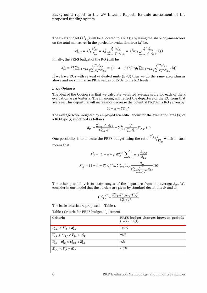
The other possibility is to state ranges of the departure from the average 𝐸!". We consider in our model that the borders are given by standard deviations d+ and d-.

𝑑!,!!!=

!!!!! !!,!,!

! !!!,!! !!!

!!!

!!!!!!!

!!!.

The basic criteria are proposed in Table 1.

Table 1 Criteria for PRFS budget adjustment Criteria PRFS budget changes between periods

(t-1) and (t).

𝑬𝒊,𝒌,𝒋𝒕 ≥ 𝑬𝒊,𝒌𝒕 + 𝒅𝒊,𝒌𝒕 +10%

𝑬𝒊,𝒌𝒕 ≤ 𝑬𝒊,𝒌,𝒋

𝒕 < 𝑬𝒊,𝒌 + 𝒅𝒊,𝒌𝒕 +5%

𝑬𝒊,𝒌𝒕 − 𝒅𝒊,𝒌𝒕 < 𝑬𝒊,𝒌,𝒋𝒕 < 𝑬𝒊,𝒌𝒕 -5%

𝑬𝒊,𝒌,𝒋𝒕 < 𝑬𝒊,𝒌𝒕 − 𝒅𝒊,𝒌𝒕 -10%



The budget changes can be evaluation area specific, in this case the table will have 6 columns.

Because it is very unlikely that the distribution of evaluation scores will be fully symmetric we need to recalculate the primarily allocated PRFS to the level of actually available budget. Denote 𝑋!..! the budget calculated by (6) or by using Table 1. Then

𝑋!! = 𝑋!,!!!!!!! and 𝑋!,!! = 𝑋!,!,!!!

!!!

To make the LHS of equation (6) or its modification using Table 1 being equal 𝑋!! as

defined in equation (1) we have to multiply the RHS of (6) by the ratio 𝑋!!

𝑋!!. We have

the initial PRFS change

𝑋!,!,!! = 𝜖!,!,!! 1 − 𝛼 − 𝛽 𝑌!,!!!!𝑤!,!𝑔!,

where 𝜖!,!,!! is the actual engine of the budget change given by either 𝐸!,!,!!

𝐸!,!! or by

rules of Table 1. Consequently, we can express 𝑋!! as

𝑋!! = 𝑋!,!,!!!!!!

!!!!! = 1 − 𝛼 − 𝛽 𝑔! 𝑌!,!!!! 𝜖!,!,!! 𝑤!,!!

!!!!!!!!

Using equation (2) for 𝑋!! we yield !!!

!!! =

(!!!!!)!!!!!!!

!!!!! !! !!,!!!! !!"#

! !!,!!!!!

!!!!!

= !!!!!

!!,!!!! !!"#

! !!,!!!!!

!!!!!

. (7)

Alternatively, the budget can be balanced in each social priority (evaluation area).

If a RO has more than on EvU an RU, we need first to aggregate the evaluations in each category to the RO level using relative size of EvUs or RUs (the shares of scientific staff on the total staff).

2.1.4 Relationship between Option 1 and Option 2.

Below we use Option 2 in the mode using 𝐸!,!,!!

𝐸!,!!to determine PRFS. The implication

for the mode using Table 1 is straightforward.

Equation (3) of Option 1 can be rewritten as

𝑋!,!,!! = 𝑋!!𝑤!,!!!!!!!!,!,!

!

!!!!!!!,!,!

!!!!!!

= 𝑋!!𝑤!,!

!!!!!

!!!!!!!

!!!!!,!,!!

!!!!!

!!!!!!!

!!!!!,!,!!!!

!!!

= 𝑋!!!!!!!

!!!!!!!

!!!𝑤!,!

!!,!,!!

!!!!!

!!!!!!!

!!!!!,!,!!!!

!!!

And consequently (4) will have now the form

𝑋!,!! = 𝑋!!!!!!!

!!!!!!!

!!!𝑤!,!

!!,!,!!

!!!!!

!!!!!!!

!!!!!,!,!!!!

!!!

!!!! =

!!!!!

!!!!!!!

!!!(1 − 𝛼 − 𝛽)𝑌!!!!𝑔! 𝑤!,!

!!,!,!!

!!!!!

!!!!!!!

!!!!!,!,!!!!

!!!

!!!! (9)

The similarity and the difference between equations (6) and (9) is evident. Denote 𝑍!,!! the sum in (6) and (9)



𝑍!,!! = 𝑤!,!𝐸!"#!

𝐿!!!!

𝐿!!!!!!!!!

𝐸!,!,!!!!!!!

!

!!!

Using it we can write equation (9) i.e. the PRFS of the RO j given by Option 1 as

𝑋!,!!,! = (1 − 𝛼 − 𝛽)𝑌!!!!𝑔!

!!!!!

!!!!!!!

!!!𝑍!,!! . (10)

Now, we concentrate on Option 2. Equation (6) can be recalculated by (7) and thus

𝑋!,!!!,! =

1 − 𝛼 − 𝛽 𝑌!!!!𝑔!1 − 𝛼 − 𝛽 𝑔! 𝑌!,!!!! 𝜖!"#! 𝑤!,!!

!!!!!!!!

1 − 𝛼 − 𝛽 𝑌!,!!!!𝑔!𝑍!,!!

𝑋!,!!!,! = !!

!!!

!!,!!!!!!,!

!!!!!!

(1 − 𝛼 − 𝛽)𝑌!,!!!!𝑔!𝑍!,!! . (11)

Comparing equations (10) and (11) we get the notion about the differences between the two methods: Option 1 and Option 2. 𝑍!,!! is the relative position of an EvU in the evaluation in the corresponding RO type and is common to the both formulas. In Option 1 this is multiplied by the budget allocated to the RO or EvU by its relative size (within the corresponding RO type). In Option 2 it is multiplied by the previous period budget corrected to the overall available budget. In this case, the size does not matter while the base year (and then always the previous period) IF of the RO matters.

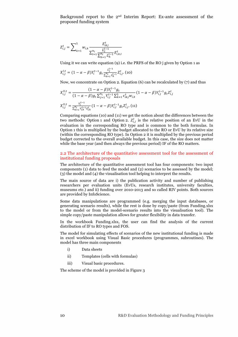
2.2 The architecture of the quantitative assessment tool for the assessment of institutional funding proposals The architecture of the quantitative assessment tool has four components: two input components (1) data to feed the model and (2) scenarios to be assessed by the model; (3) the model and (4) the visualisation tool helping to interpret the results.

The main source of data are i) the publication activity and number of publishing researchers per evaluation units (EvUs, research institutes, university faculties, museums etc.) and ii) funding over 2010-2013 and so called RIV points. Both sources are provided by InfoScience.

Some data manipulations are programmed (e.g. merging the input databases, or generating scenario results), while the rest is done by copy/paste (from Funding.xlsx to the model or from the model-scenario results into the visualisation tool). The simple copy/paste manipulation allows for greater flexibility in data transfer.

In the workbook Funding.xlsx, the user can find the analysis of the current distribution of IF to RO types and FOS.

The model for simulating effects of scenarios of the new institutional funding is made in excel workbook using Visual Basic procedures (programmes, subroutines). The model has three main components

i) Data sheets

ii) Templates (cells with formulas)

iii) Visual basic procedures.

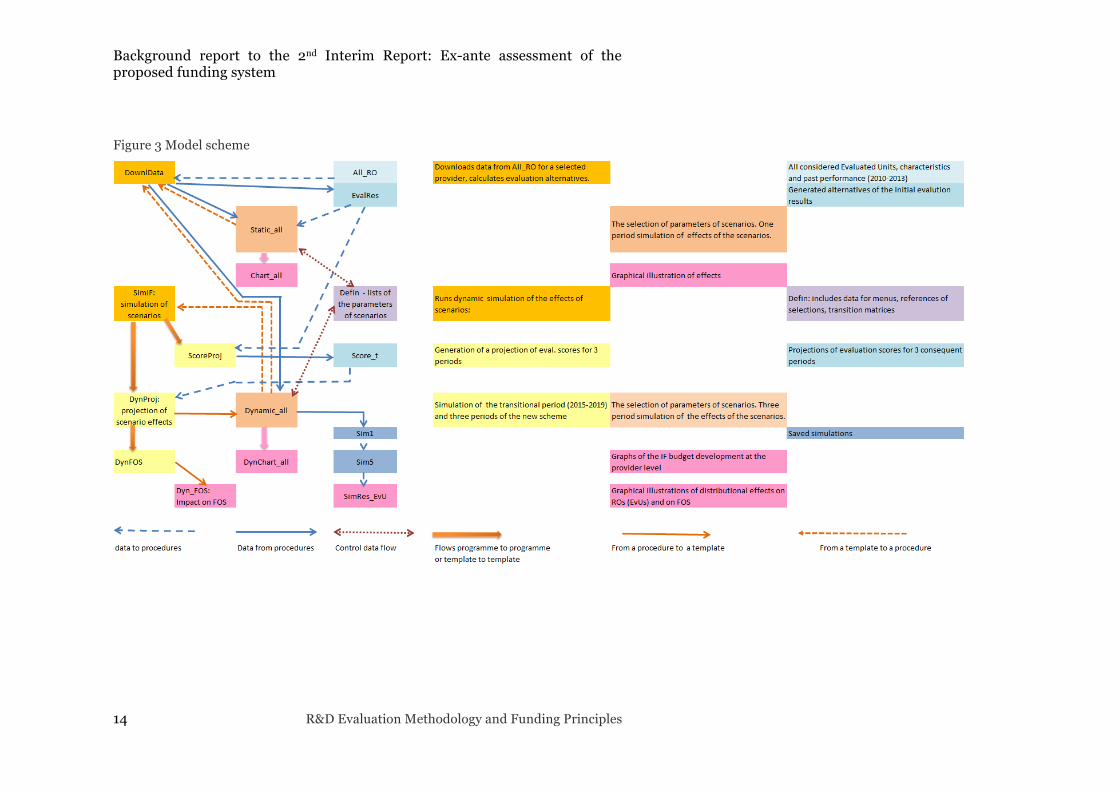
The scheme of the model is provided in Figure 3



Figure 2 Basic architecture of the quantitative tool

2.3 Parameters to be specified While the principles of funding are described in WP7 Report and the methodology is mathematically stated in Paragraph 2.2., to assess the effects we need to know concrete implementation parameters and the evaluation results. They are summarised in Table 2

Table 2 Implementation parameters to be specified

Parameters to be specified Corresponding to

Division of the IF into three components: base IF, PA, PRFS

≈ stability of the financing; responsiveness to the performance

The weights of the evaluation criteria for each RO type

≈ social preferences, what is expected from each RO type

Base year, transition period (if any) ≈ IF is set on recent history

Budget changes (decline, no change, growth) ≈budget allocations to providers

Scientific staff considered and its development ≈ it is a weighting factor for calculating totals for IF providers, PRFS is distributed according it in Option 1



Evidently, most of these parameters will be subject of further analyses, negotiations with stakeholders and in the end they will have to be stated by policy makers. To make the assessment easier we make assumptions about some of them, and these assumptions are not alternate in scenarios.

1) The base year is set to 2013, and no changes are considered before launching the new scheme.

2) In this report we do not consider changes in the IF budget allocated to providers, i.e. the changes will happen only among ROs within the competence area of a provider and only due to the evaluation and the IF allocation methods.

3) Bearing in mind the discussion and proposals how to define, gather and use scientific labour figures, we use the estimates provided by InfoScience based on publication activities during the period 2010-2013 as a proxy for FTE researchers. We are aware that these figures are given in terms of head counts and that in reality FTE might be much lower in some ROs.



Figure 3 Model scheme



In this report we also do not alternate the distribution between the three components of IF. We consider 80% of the base year budget being translated in the Block Financing, 5% will be given to the Performance Agreements and 15 % will constitute PRFS. Nevertheless, we suppose that in future it will be a subject of further scenarios following the likely discussion on it.

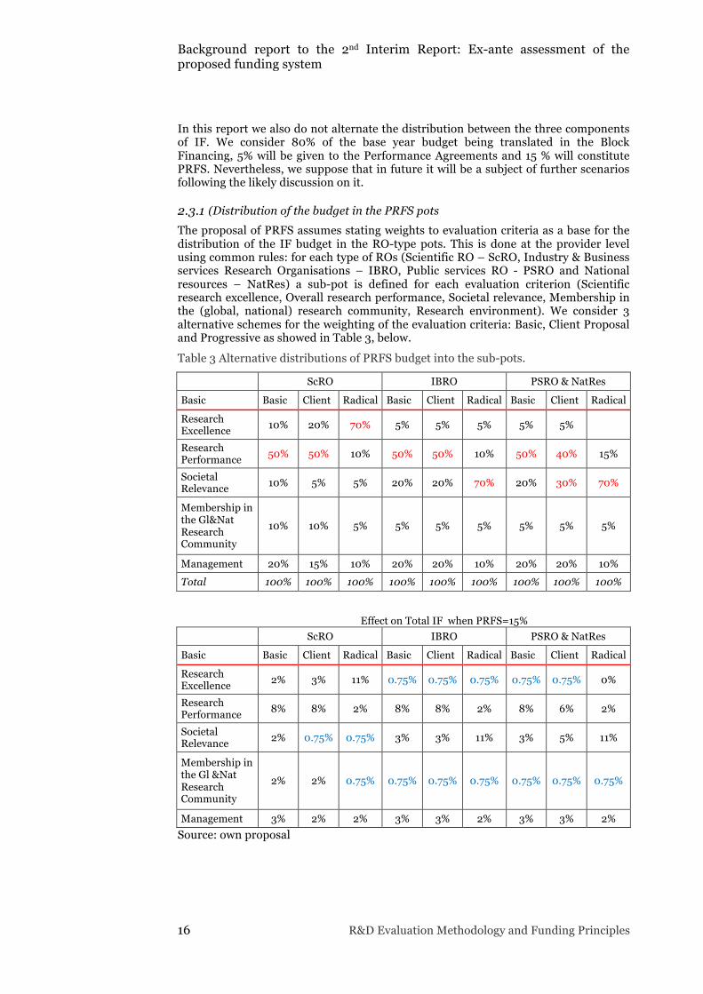
2.3.1 (Distribution of the budget in the PRFS pots The proposal of PRFS assumes stating weights to evaluation criteria as a base for the distribution of the IF budget in the RO-type pots. This is done at the provider level using common rules: for each type of ROs (Scientific RO – ScRO, Industry & Business services Research Organisations – IBRO, Public services RO - PSRO and National resources – NatRes) a sub-pot is defined for each evaluation criterion (Scientific research excellence, Overall research performance, Societal relevance, Membership in the (global, national) research community, Research environment). We consider 3 alternative schemes for the weighting of the evaluation criteria: Basic, Client Proposal and Progressive as showed in Table 3, below.

Table 3 Alternative distributions of PRFS budget into the sub-pots.

ScRO IBRO PSRO & NatRes

Basic Basic Client Radical Basic Client Radical Basic Client Radical

Research Excellence 10% 20% 70% 5% 5% 5% 5% 5%

Research Performance 50% 50% 10% 50% 50% 10% 50% 40% 15%

Societal Relevance 10% 5% 5% 20% 20% 70% 20% 30% 70%

Membership in the Gl&Nat Research Community

10% 10% 5% 5% 5% 5% 5% 5% 5%

Management 20% 15% 10% 20% 20% 10% 20% 20% 10%

Total 100% 100% 100% 100% 100% 100% 100% 100% 100%

Effect on Total IF when PRFS=15%

ScRO IBRO PSRO & NatRes

Basic Basic Client Radical Basic Client Radical Basic Client Radical

Research Excellence 2% 3% 11% 0.75% 0.75% 0.75% 0.75% 0.75% 0%

Research Performance 8% 8% 2% 8% 8% 2% 8% 6% 2%

Societal Relevance 2% 0.75% 0.75% 3% 3% 11% 3% 5% 11%

Membership in the Gl &Nat Research Community

2% 2% 0.75% 0.75% 0.75% 0.75% 0.75% 0.75% 0.75%

Management 3% 2% 2% 3% 3% 2% 3% 3% 2% Source: own proposal



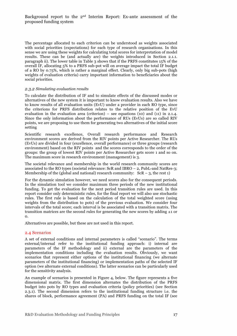
The percentage allocated to each criterion can be understood as weights associated with social priorities (expectations) for each type of research organisations. In this sense we are using these weights for calculating total scores for interpretation of model results. These can be (and actually are) the weights introduced in Section 2.1.1. paragraph ii). The lower table in Table 3 shows that if the PRFS constitutes 15% of the overall IF, allocating 5% to a PRFS sub-pot will on average impact the total IF budget of a RO by 0.75%, which is rather a marginal effect. Clearly, only big sub-pots (high weights of evaluation criteria) carry important information to beneficiaries about the social priorities.

2.3.2 Simulating evaluation results To calculate the distribution of IF and to simulate effects of the discussed modes or alternatives of the new system it is important to know evaluation results. Also we have to know results of all evaluation units (EvU) under a provider in each RO type, since the criterions for PRFS distribution relates to the relative position of the EvU evaluation in the evaluation area (criterion) – see equations (10) and (11) in 2.1.4. Since the only information about the performance of RUs (EvUs) are so called RIV points, we are proposing to use them for generating two alternatives of the initial score setting

Scientific research excellence, Overall research performance and Research environment scores are derived from the RIV points per Active Researcher. The RUs (EvUs) are divided in four (excellence, overall performance) or three groups (research environment) based on the RIV points and the scores corresponds to the order of the groups: the group of lowest RIV points per Active Researcher gets score 1 and so on. The maximum score in research environment (management) is 3.

The societal relevance and membership in the world research community scores are associated to the RO types (societal relevance: ScR and IBRO – 2, PubL-and NatRes-3; Membership of the (global and national) research community: ScR – 3, the rest 1)

For the dynamic simulation however, we need scores also for the consequent periods. In the simulation tool we consider maximum three periods of the new institutional funding. To get the evaluation for the next period transition rules are used. In this report consider only deterministic rules, for the final report we will also use stochastic rules. The first rule is based on the calculation of the total weighted score (using weights from the distribution to pots) of the previous evaluation. We consider four intervals of the total score; each interval is be associated with a transition matrix. The transition matrices are the second rules for generating the new scores by adding ±1 or 0.

Alternatives are possible, but these are not used in this report.

2.4 Scenarios A set of external conditions and internal parameters is called “scenario”. The terms external/internal refer to the institutional funding approach: i) internal are parameters of the IF methodology and ii) external are the parameters of the implementation conditions including the evaluation results. Obviously, we want scenarios that represent either options of the institutional financing (we alternate parameters of the institutional financing) or implementation paths of the selected IF option (we alternate external conditions). The latter scenarios can be particularly used for the sensitivity analysis.

An example of scenarios is presented in Figure 4, below. The figure represents a five dimensional matrix. The first dimension alternates the distribution of the PRFS budget into pots by RO types and evaluation criteria (policy priorities) (see Section 2.3.1). The second dimension refers to the institutional funding structure i.e. the shares of block, performance agreement (PA) and PRFS funding on the total IF (see



Figure 1)). Two alternatives are considered. From the decision making point of view these two dimensions should be switched in the order. These first three dimensions refer to the internal (IF) parameter setting. The fourth dimension refers to the development of evaluation results over time i.e. to the selection of transition matrices (see 0, the last paragraph). The fifth dimension refers to time – we consider three consequent periods.

In this report we run and analyse scenarios given by the alternative setting of pot weight/

2.5 Running simulations The simulation is fully programmed in Visual Basic. Each change of parameters calls the routine SimIF and hence the scenario is updated.

Scenarios are created interactively by users. Storing modifications of individual parameters allow for creating more complex scenarios differing in more than one parameter setting. Scenario parameters are displayed in the simulation sheets. Up to 6 scenario results can be stored in the excel workbook.

Up to 3 scenarios (of 6 stored) can be compared in the sheets SimRes_EvU sheet. The comparison is controlled by scroll-boxes (period in which the comparison will happen, scenarios to be compared, variables/IF-component to be compared/displayed and the comparison base i.e. Total IF or PRFS).



Figure 4 An example of scenarios

Dimension 1

Dimension 2

Dimension 3

Dimension 4

Dimension 5



2.6 Visualisation of the results While the overall budget for IF will not be affected by the proposed methodology, the effects of the new IF system are distributional i.e. some ROs might benefit and some might lose due to the introduction of the new scheme or due to the changes of parameters of the new scheme. In order to enable an easy analysis of the distributional effect we prepared a visualisation tool developed in Java script. It is available as a web application. The tool is built upon a collection of scenario-model runs. The user by clicking on the buttons selects scenarios and sees the effects in the chart on the screen.

The mechanism of visualization is known as a pack layout. The smaller circles (leafs) represent the research fields (RF). The surface area (size) of the RFs is a function of IF distribution according to a particular scenario. By default, the size of RFs reflects the distribution of IF budget in 2019. The circles are fully comparable at this level and are sorted in descending order following a spiral path. RFs are further nested within the research areas (RA). While the RFs are comparable within and also across the RAs, the larger circles representing the RAs are not mutually comparable. They are correctly sorted in descending order according to the sum of respective RFs; nevertheless, the size of the larger circles depends not only on the aggregation of the RFs but also on a space used by the smaller circles. The degree of a wasted space is different across the RAs and is related to a number of smaller circles (RFs) and their circle size variability. This is a prize for more illustrative hierarchy description and transition features compared to other competitive layouts (e.g. a treemap). The actual amount of IF (in thousands CZK) can be obtained as a mouse-over tooltip for a given RF. Moreover, the zoom function is also available for the main window.

Each RF is described by an acronym which is equivalent to the long field classification used for the IPN Metodika project. Few fields are not included in the visualization because of its marginal role. For simplicity, the present simulation is based on assumption of max. 2 RFs within a given RO. This assumption is quite restrictive but can be easily relaxed if necessary. Before clicking the update buttons, one could consult the detailed legend by clicking on the link situated above the buttons at the top of the page. The legend describes values of all parameters described elsewhere. The combination of all their values results in 2×2×3×3×3=108 buttons representing IF scenarios. The darker the button’s colour, the lower the correlation with the baseline value and, thus, the higher degree of transitions in order at both RA and RF levels.



3. Results of the simulations

3.1 Investigated issues The purpose of building the model stated in the terms of reference is to assess the impact of the new system of institutional financing of ROs and to assess the robustness of the proposed methodology through sensitivity analysis. In this section we present and analyse some issues which popped up in the course of the development of the methodology:

• The distribution of the PRFS budget into sub-pots (Section 2.3.1) is to be decided by policy makers based on R&D policy objectives and an analysis conducted for this purpose. It is however, a challenging issue that is receiving a lot of attention in the discussion on the new IF methodology. For this reason we are showing the implications of alternating the weights. We are considering three scenarios to indicate the sensitivity of the final institutional funding distribution (PRFS) to different distributions into sub-pots as introduced in Section 2.3.1 (for the justification of the proposed distribution scenarios see Section 3.4.1 in the 2nd Interim Report).

• While so called RIV points incorporate the both aspects necessary for the distribution of IF, i.e. the quality of research performance and the size of the evaluated entity, the scores provided by the new evaluation process will lack the size dimension. This is because the current system rests largely on collecting research results, translating quantity in quality by associating outputs with values (points) in each output category. The new system is purely qualitative, quantitative indicators only feed qualitative judgements. The qualitative judgements are appraised by panels giving marks (scores 0 to 4). The report on the IF methodology addresses the need for “size” in two ways: Option A – using scientific staff (active researchers, AR) as the measurement of size relevant to IF; and Option B – accepting the base year institutional financing as the measurement of size (see the Section 3.4.2 in the 2nd Interim Report for more details)

Using scientific staff for the translation of the evaluation scores into funding (Option 1) is not without problems due to

i) Lack of reliable information on it (solutions are proposed in the 2nd Interim report)

ii) It might carry with it unpleasant effects that high figures of scientific staff can outweigh poor performance.

iii) The different notion of size in the current methodology and the proposed Option 1 will inevitably generate effects similar to (ii.).

• The range of scientific quality differentiation is much larger using RIV points (for example RIV points per active researcher (RIVpt/AR) range from 4 to 432 in the set of ROs under the IF umbrella of MEYS, while the maximum range of evaluation scores is 0 to 4, realistically between 1 and 4. As mentioned earlier, one option how to address it is to use non-linear transformation favouring better performances.

In order to demonstrate the above effects we do not assume in our analysis any growth of the IF and PRFS budgets during the investigated periods. Almost exclusively we use the basic scheme of the division of the IF components: Block IF 80%, PA 5% and PRFS 15%.



3.2 Scenarios for the distribution of the funding in the PRFS sub-pots Evidently, the distribution of PRFS into pots by RO types and sub-pots for the evaluation criteria (social preferences) must have some impact on the distribution of institutional funding. In the analysis in this chapter we consider three scenarios of such distribution into the sub-pots (Basic, Client proposed and Radical) and the two PRFS methods: Option 1 (based on person-scores) and Option 2 (based on relative scores). The PRFS sub-pots scenarios are given in Table 3 in Paragraph 2.3.1, above.

These three scenarios try to illustrate some possible views on the performance of ROs and its steering:

• Basic distribution: in this scenario the policy aim at enhancing the Overall performance as an absolute base for the development of Czech science, while the other criteria should moderately contribute to it.

• Radical scenario: ROs should be guided to improve in the areas of their main mission i.e. ScRO in Scientific Research Excellence, and all the other RO types in Social Relevance.

• Client scenario: reflects an opinion of a stakeholder; it is a modification of the Basic distribution, putting slightly more emphasis on the areas of the main mission of RO types (like in the radical scenario).

The effects of these scenarios are illustrated by comparing Client and Radical scenarios to the basic scenario. To do the comparison, we use two indicators

• The average relative deviation, where the relative deviation is calculated for each RO and refers to the ratio of the absolute difference between PRFS values between the compared and basic scenario over the PRFS allocation in the Basic scenario.

• The absolute deviation, but instead of its average we use standard deviation as used in statistics; these are expressed in thousand Czech Crowns.

In addition we present maximum deviations in relative and absolute terms.

Looking at the results using Option 1 PRFS (Table 4) we see that difference between the Basic and Client scenarios is rather small; on average 3% with the maximum of 8% in the first period, and these figures only moderately change in the next two periods. There are quite a few ROs (EvUs) for which the change is below 1%: 44% in the first period and 33% in the second period. In absolute terms the maximum deviation of the Client scenario from the basic one accounts for a million crowns, the average is just only about 16 thousand crowns.

Table 4 Comparison of scenario in respect to the Basic scenario. (Option 1 PRFS)

PRFS Average absolute deviation

Period 1 Period 2 Period 3

# 1-client 1-radical 1-client 1-radical 1-client 1-radical

Min dev. 0% 0% 0% 0% 0% 0%

Max dev. 8% 29% 14% 78% 13% 87%

Avg 180 3% 9% 4% 32% 4% 35%

# for dev.<1% 44% 1% 33% 1% 8% 8%



PRFS Absolute deviation



CZK'000 CZK'000 CZK'000 CZK'000 CZK'000 CZK'000

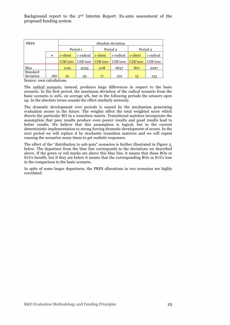
Max 1129 4035 1118 6637 807 9297 Standard deviation 180 16 59 17 120 15 133

Source: own calculations

The radical scenario, instead, produces large differences in respect to the basic scenario. In the first period, the maximum deviation of the radical scenario from the basic scenario is 29%, on average 9%, but in the following periods the scissors open up. In the absolute terms sounds the effect similarly seriously.

The dramatic development over periods is caused by the mechanism generating evaluation scores in the future. The weights affect the total weighted score which directs the particular RO in a transition matrix. Transitional matrices incorporate the assumption that poor results produce even poorer results and good results lead to better results. We believe that this assumption is logical, but in the current deterministic implementation to strong forcing dramatic development of scores. In the next period we will replace it by stochastic transition matrices and we will repeat running the scenarios many times to get realistic responses.

The effect of the “distribution to sub-pots” scenarios is further illustrated in Figure 5, below. The departure from the blue line corresponds to the deviations we described above. If the green or red marks are above this blue line, it means that these ROs or EvUs benefit, but if they are below it means that the corresponding ROs or EvUs lose in the comparison to the basic scenario.

In spite of some larger departures, the PRFS allocations in two scenarios are highly correlated.



Figure 5 Comparison of the Client and Radical scenarios in respect to the Basic scenario. (Option 1 PRFS, period 1)

In the sample of ROs we model the impacts for three types of organisations ScRO (169), PSRO (10) and NatRes (1). The proposed mechanism does not allow changing PRFS of a member of a single organisation group (NatRes in our case), thus there is nothing to report.

Table 5 shows the separate effects within the groups of ScRO and PSRO in relative terms in the first period. In general, the effects are slightly more moderate for PSRO except for the average relative absolute deviation in te radical scenario when the percentage for PSRO is larger than for ScRO (likely also because the PSRO group is much smaller). .

Table 5 Comparison of scenario in respect to the Basic scenario. (Option 1 PRFS, period 1) – differentiated by RO types.

PRFS Average relative absolute deviation

ScRO PSRO

# 1-client 1-radical # 1-client 1-radical

Min 1% 3% 0% 2%

Max 8% 29% 4% 20%

Avg 169 3% 9% 10 2% 12% Source: own calculations

When using Option 2 PRFS, i.e. the relative scores, we see similar results when comparing the “distribution to sub-pots” scenarios. These are summarised in Table 6. In this case, results are provided at the ROs’ level. Note that the standard deviation is in this case bigger, because the ROs are bigger (aggregates of EvUs).



The Client scenario exhibits only moderate departures from the Basic scenario, while the Radical one deviates significantly. In other words, the earlier stated judgements hold also for the Option 2.

Table 6 Comparison of scenario in respect to the Basic scenario. (Option 2 PRFS)

PRFS Average relative deviation



Min 0% 0% 0% 0% 0% 0%

Max 7% 29% 12% 67% 10% 68%

Avg 33 2% 7% 3% 17% 3% 19%

# for dev.<1% 39% 6% 27% 3% 9% 6%

PRFS Absolute deviation



CZK'000 CZK'000 CZK'000 CZK'000 CZK'000 CZK'000

Max 2537 12869 1904 9273 1618 9045 Standard deviation 33 86 434 85 508 90 596

Source: own calculation

If we compare the total institutional funding of the selected scenarios (Table 7) we find that the effects are rather small. It holds particularly for the Client scenario where the deviations from the Basic scenario do not exceed 1% in the first year and 2% in the next periods. The effects of the Radical scenario are more pronounced, but still rather moderate.

Table 7 Comparison of scenario in respect to the Basic scenario. (Option 1 PRFS) – total IF

Total IF Average relative deviation



Min 0% 0% 0% 0% 0% 0%

Max 1% 3% 1% 8% 2% 13%

Avg 33 0.2% 1% 1% 3% 1% 5%

# for dev.<1% 100% 67% 85% 12% 73% 6%

Source: own calculation



3.3 The size effect in the Option 1 approach to PRFS (person-scores)

3.3.1 The roots of the problem We focused our analysis on the ROs funded by the MEYS. The ROs are anonymised in order to avoid readers’ concentration on evaluation results which are developed purely for the testing of the system and do not constitute predictions.

The sample includes ROs of various sizes and of three types: scientific research organisations (1 research institute and 21 universities) – referenced in the graph as ScRO, public service ROs (10) – referenced as PubL, and an infrastructure RO (1)- referenced as NatRes.

The chart below (Figure 6) provides insight in the problem arising with the principal change of the IF methodology. It is clear that there are some unexpected distributional effects. The “PubL1” gains markedly (20% in terms of total IF) while its evaluation score is rather average (2.2) while the ROs “Publ2” and “Publ3” lose 4 and 5 per cent respectively with the top total score (3.5). We can find similar contrasting cases among the universities too: average performing universities (with the scores about 2.4) “ScRO2U” – “ScRO4U” lose from -3 to -2 percent of total IF, while the badly performing university “ScRO7U” (the total score 1.3) gains 8% on total IF.

Figure 6 Total (average) scores and percentage change of total IF

Note: Total score: scores weighted by the “pot weights” and by active researchers within the ROs with several EvUs. The affix “U” in the RO name indicates that the RO is university. Scenario: IF components [80%, 5%, 15%]; Basic scheme for distr. to pots; linear transformation of scores; evaluation alternative: scores proportional to RIV/AR; It can be shown that these strange effects can also be observed for other evaluation score alternatives.

In Figure 7, below, we present some further details on the relationship between the scores and the allocations of institutional financing.

First, we concentrate on the distribution of PRFS funds, since the block and PA components are predetermined as 85% of the base year IF. In the right chart of Figure



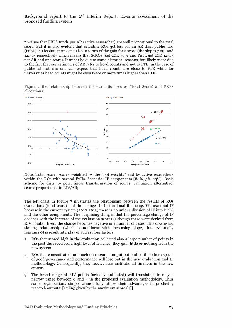
7 we see that PRFS funds per AR (active researcher) are well proportional to the total score. But it is also evident that scientific ROs get less for an AR than public labs (PubL) in absolute terms and also in terms of the gain for a score (the slopes 7.691 and 12.375 respectively which means that ScROs get CZK 7691 and PubL get CZK 12375 per AR and one score). It might be due to some historical reasons, but likely more due to the fact that our estimates of AR refer to head counts and not to FTE; in the case of public laboratories one can expect that head counts are close to FTE while for universities head counts might be even twice or more times higher than FTE.

Figure 7 the relationship between the evaluation scores (Total Score) and PRFS allocations

Note: Total score: scores weighted by the “pot weights” and by active researchers within the ROs with several EvUs. Scenario: IF components [80%, 5%, 15%]; Basic scheme for distr. to pots; linear transformation of scores; evaluation alternative: scores proportional to RIV/AR;

The left chart in Figure 7 illustrates the relationship between the results of ROs evaluations (total score) and the changes in institutional financing. We use total IF because in the current system (2010-2013) there is no unique division of IF into PRFS and the other components. The surprising thing is that the percentage change of IF declines with the increase of the evaluation scores (although these were derived from RIV points). Even, the change becomes negative in a number of cases. This downward sloping relationship (which is nonlinear with increasing slope, thus eventually reaching 0) is result interplay of at least four factors:

1. ROs that scored high in the evaluation collected also a large number of points in the past thus received a high level of I; hence, they gain little or nothing from the new system.

2. ROs that concentrated too much on research output but omited the other aspects of good governance and performance will lose out in the new evaluation and IF methodology. Consequently, they receive less institutional finances in the new system.

3. The broad range of RIV points (actually unlimited) will translate into only a narrow range between 0 and 4 in the proposed evaluation methodology. Thus some organisations simply cannot fully utilise their advantages in producing research outputs; [ceiling given by the maximum score (4)].



4. ROs with a low intensity of RIV points (i.e. low RIV/AR) will gain when even low scores of their narrow range are assigned to all active researchers; [different implementation of size criteria in the financing methodology].

Because the budget is limited, in order someone to gain some other must lose. Those who gain little in the evaluation might even turn into a loser.

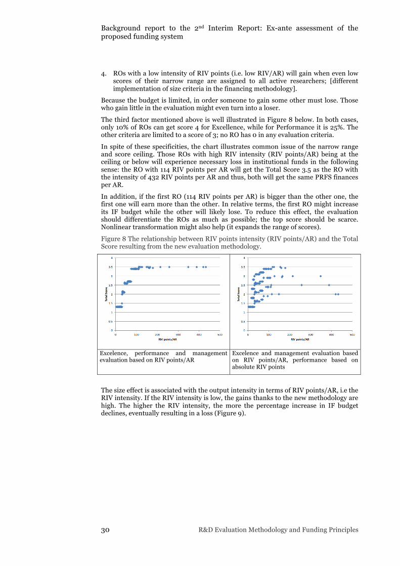
The third factor mentioned above is well illustrated in Figure 8 below. In both cases, only 10% of ROs can get score 4 for Excellence, while for Performance it is 25%. The other criteria are limited to a score of 3; no RO has 0 in any evaluation criteria.

In spite of these specificities, the chart illustrates common issue of the narrow range and score ceiling. Those ROs with high RIV intensity (RIV points/AR) being at the ceiling or below will experience necessary loss in institutional funds in the following sense: the RO with 114 RIV points per AR will get the Total Score 3.5 as the RO with the intensity of 432 RIV points per AR and thus, both will get the same PRFS finances per AR.

In addition, if the first RO (114 RIV points per AR) is bigger than the other one, the first one will earn more than the other. In relative terms, the first RO might increase its IF budget while the other will likely lose. To reduce this effect, the evaluation should differentiate the ROs as much as possible; the top score should be scarce. Nonlinear transformation might also help (it expands the range of scores).

Figure 8 The relationship between RIV points intensity (RIV points/AR) and the Total Score resulting from the new evaluation methodology.

Excelence, performance and management evaluation based on RIV points/AR

Excelence and management evaluation based on RIV points/AR, performance based on absolute RIV points

The size effect is associated with the output intensity in terms of RIV points/AR, i.e the RIV intensity. If the RIV intensity is low, the gains thanks to the new methodology are high. The higher the RIV intensity, the more the percentage increase in IF budget declines, eventually resulting in a loss (Figure 9).



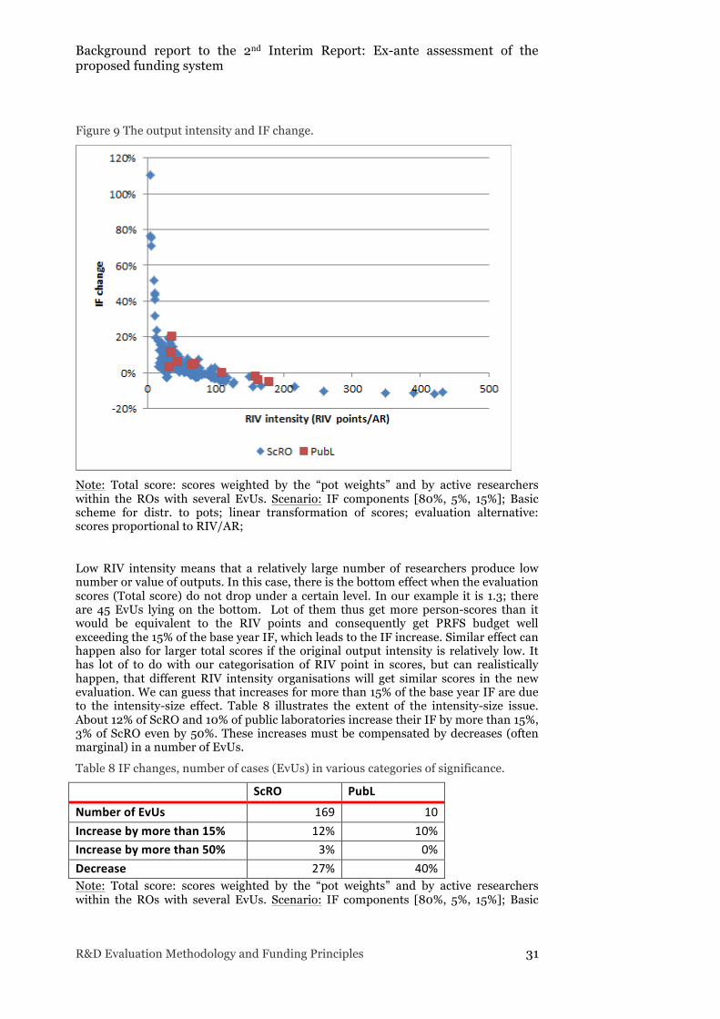
Figure 9 The output intensity and IF change.

Note: Total score: scores weighted by the “pot weights” and by active researchers within the ROs with several EvUs. Scenario: IF components [80%, 5%, 15%]; Basic scheme for distr. to pots; linear transformation of scores; evaluation alternative: scores proportional to RIV/AR;

Low RIV intensity means that a relatively large number of researchers produce low number or value of outputs. In this case, there is the bottom effect when the evaluation scores (Total score) do not drop under a certain level. In our example it is 1.3; there are 45 EvUs lying on the bottom. Lot of them thus get more person-scores than it would be equivalent to the RIV points and consequently get PRFS budget well exceeding the 15% of the base year IF, which leads to the IF increase. Similar effect can happen also for larger total scores if the original output intensity is relatively low. It has lot of to do with our categorisation of RIV point in scores, but can realistically happen, that different RIV intensity organisations will get similar scores in the new evaluation. We can guess that increases for more than 15% of the base year IF are due to the intensity-size effect. Table 8 illustrates the extent of the intensity-size issue. About 12% of ScRO and 10% of public laboratories increase their IF by more than 15%, 3% of ScRO even by 50%. These increases must be compensated by decreases (often marginal) in a number of EvUs.

Table 8 IF changes, number of cases (EvUs) in various categories of significance.

ScRO PubL

Number of EvUs 169 10 Increase by more than 15% 12% 10% Increase by more than 50% 3% 0% Decrease 27% 40% Note: Total score: scores weighted by the “pot weights” and by active researchers within the ROs with several EvUs. Scenario: IF components [80%, 5%, 15%]; Basic



scheme for distr. to pots; linear transformation of scores; evaluation alternative: scores proportional to RIV/AR;

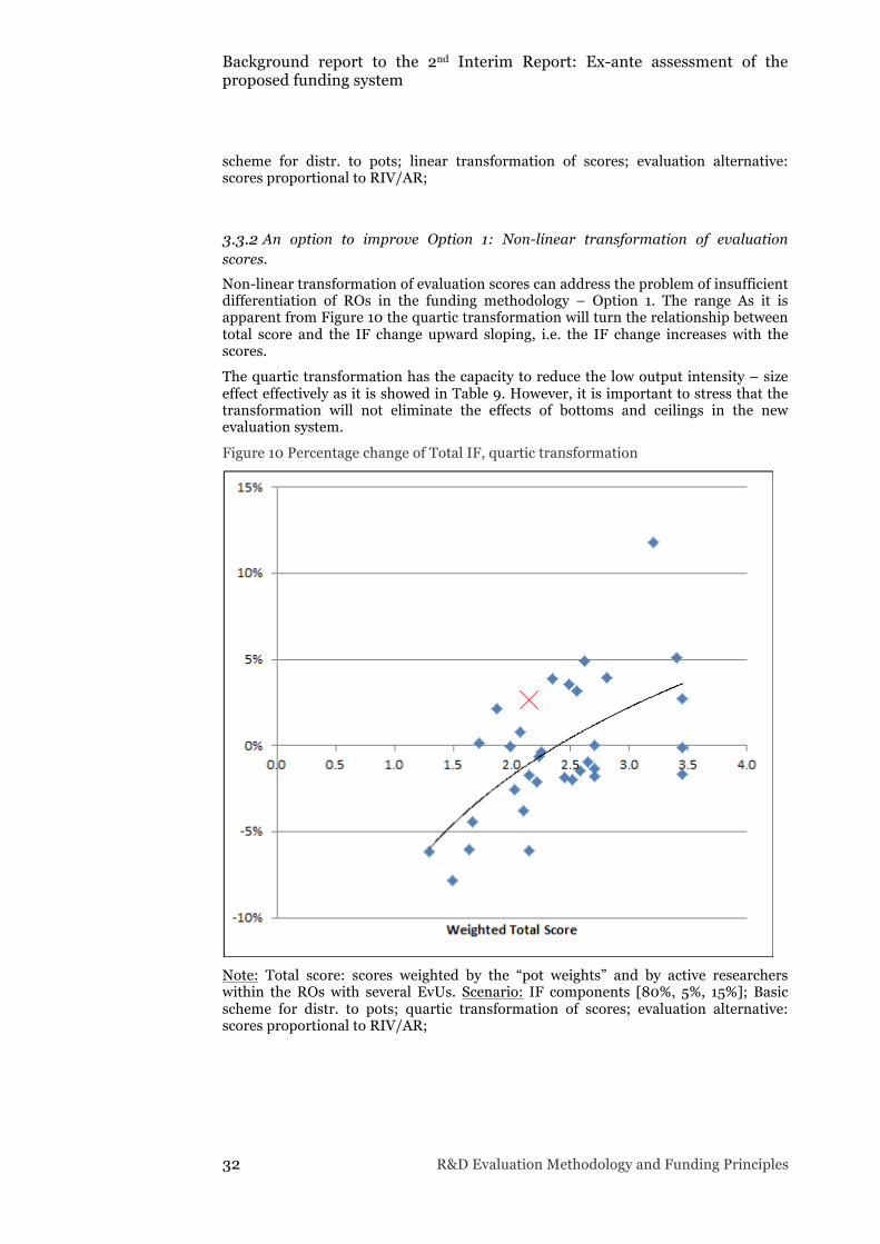
3.3.2 An option to improve Option 1: Non-linear transformation of evaluation scores. Non-linear transformation of evaluation scores can address the problem of insufficient differentiation of ROs in the funding methodology – Option 1. The range As it is apparent from Figure 10 the quartic transformation will turn the relationship between total score and the IF change upward sloping, i.e. the IF change increases with the scores.

The quartic transformation has the capacity to reduce the low output intensity – size effect effectively as it is showed in Table 9. However, it is important to stress that the transformation will not eliminate the effects of bottoms and ceilings in the new evaluation system.

Figure 10 Percentage change of Total IF, quartic transformation

Note: Total score: scores weighted by the “pot weights” and by active researchers within the ROs with several EvUs. Scenario: IF components [80%, 5%, 15%]; Basic scheme for distr. to pots; quartic transformation of scores; evaluation alternative: scores proportional to RIV/AR;



Table 9 The benefit of quartic transformation of scores

RO Total Score

Total Quartic Score

IF change

Linear T Quartic T Moderates penalisation

PubL3 3.5 173 -‐5% -‐2% PubL2 3.5 173 -‐4% 0% ScRO2U 2.4 72 -‐3% -‐2%

Rather neutral ScRO21U 2.6 67 -‐1% -‐1% PubL9 3.4 165 0% 5% ScRO11U 2.5 79 0% 3%

Offsets unexpected improvements

PubL10 2.2 28 11% -‐2% ScRO22U 1.7 18 15% 0% PubL1 2.2 28 20% 3%

3.3.3 Option 1 from the dynamic perspective The issue is if the above properties of Option 1 vanish when the financing goes from the period when PRFS has already been allocated using the results of the new evaluation methodology i.e. from Period 1 to Period 2. In order to show the net effect of the Option 1 we do assume any changes of scores between periods (from Period 1 to Period 2 and from Period 2 to Period 3). The only factor driving dynamic changes is subjecting 15% of the previous budget to the reallocation using Option 1.

Figure 11 shows that also under these circumstance the effect of Approach A in favouring small beneficiaries and penalising the large ones persists. It has also been shown that allowing 40% of IF to be allocated through the PRFS will not help; it might even lead to larger departures.



Figure 11 IF distributions in Period 2 and Period 3 relatively to IF allocations in Period 1.

Note: The level of EvUs; Total score: scores weighted by the “pot weights”;. Scenario: IF components [80%, 5%, 15%]; Basic scheme for distr. to pots; linear transformation of scores; evaluation alternative: scores proportional to RIV/AR; no dynamic changes of scores.

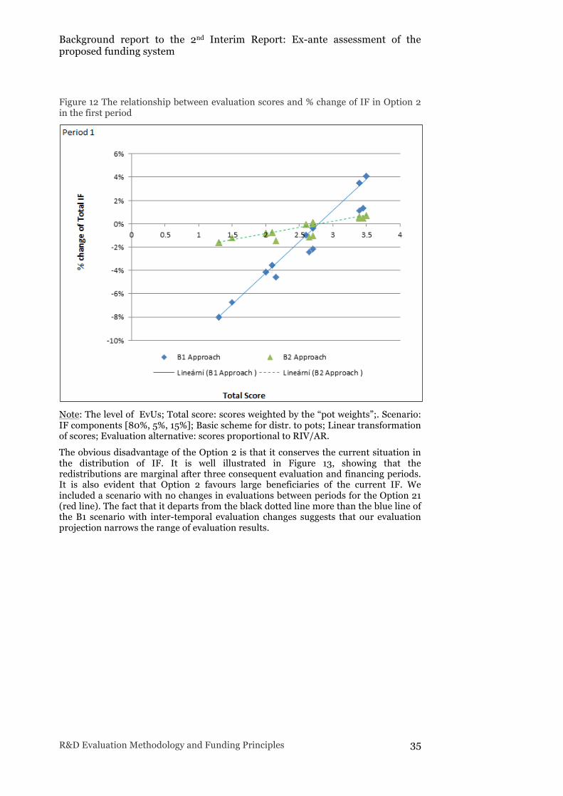
3.4 The Option 2 approach (relative scores) The two modes of PRFS Option 2 (i.e. B1 where the change of the PRFS is given by the relative position of the evaluation scores in the average scores corresponding to the respective provider, and B2 where the changes are given by Table 1 - see 2.1.2) do not differ substantially; they both follow quite closely the distribution of the IF in the base period. The differences compared to the base year IF range from -8% to 4 % for Option 2 - B1 and from -1.6% to 0.7% for Option 2 – B2 in the first period (Figure 12). The relationship between the Total Score and IF changes are more or less linear. Thus we can say that B2 is a moderate version of B1 in the current implementation; definitely B2 can be made more radical.



Figure 12 The relationship between evaluation scores and % change of IF in Option 2 in the first period

Note: The level of EvUs; Total score: scores weighted by the “pot weights”;. Scenario: IF components [80%, 5%, 15%]; Basic scheme for distr. to pots; Linear transformation of scores; Evaluation alternative: scores proportional to RIV/AR.

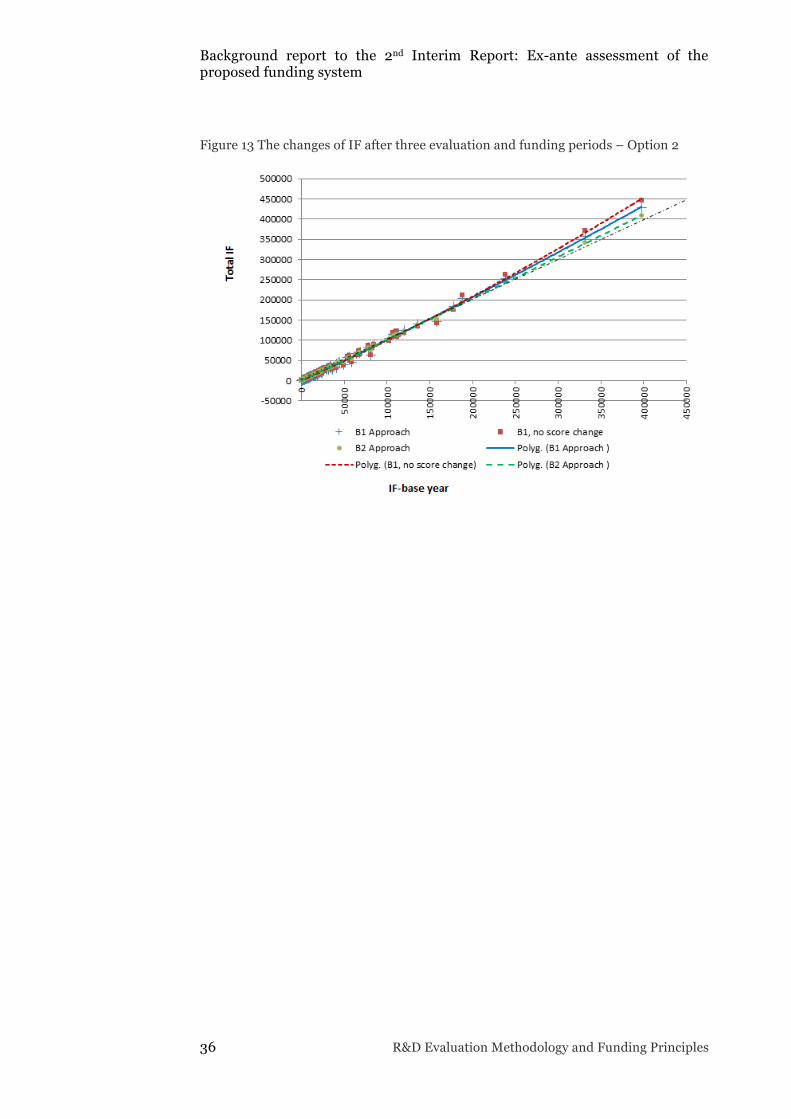
The obvious disadvantage of the Option 2 is that it conserves the current situation in the distribution of IF. It is well illustrated in Figure 13, showing that the redistributions are marginal after three consequent evaluation and financing periods. It is also evident that Option 2 favours large beneficiaries of the current IF. We included a scenario with no changes in evaluations between periods for the Option 21 (red line). The fact that it departs from the black dotted line more than the blue line of the B1 scenario with inter-temporal evaluation changes suggests that our evaluation projection narrows the range of evaluation results.



Figure 13 The changes of IF after three evaluation and funding periods – Option 2



4. Conclusions

The model appeared to be a useful instrument providing both a better insight in the funding methodology and a notion of what might be the effect of various alternatives in the parameters of the proposed funding system, which have to be stated before the system is launched.

The ex-ante analysis showed that setting weights to evaluation criteria in the funding mechanism will have important implications for the distribution of the institutional funds to ROs. In particular the so-called Radical scenario, putting a dominant emphasis on one criterion may cause a significant differentiation in institutional funding and have important consequences for the future of the ROs.

We also discussed methodological aspects in this report. Some concern the proposed methodology of PRFS allocations, others the methodology of ex-ante assessment.

Concerning the former we argue that Option 1 of PRFS allocations, i.e. based on person-scores, has the capacity to address some weaknesses of the previous system. However, exact and correct figures on scientific labour are needed; otherwise, poor performers will gain. Approach A can be improved by using a nonlinear transformation of the scores; however, it must be tailored to the actual situation.

Option 2 for the PRFS allocations, instead, based on relative scores, can well appreciate good performance and penalise poor performance. The only problem is that it might start from a bad base.

Option 2 is easy to implement while Option 1 will require substantial fine-tuning, which in return might allow for higher flexibility. For the fine-tuning, model simulations are necessary that deploy good data (otherwise garbage in, garbage out).

Concerning the latter, we suggest introducing a stochastic approach in the generation of evaluation results and then running the simulations repeatedly with the intent to estimate the mean effect of a scenario.

In collaboration with

second interim report: 3. ex-ante assessment of the proposed funding system

Education

interim report

exante assessment

evaluation scores total

new evaluation methodology

quantitative assessment

total average scores

percentage change of

prfs personscores