sebbar polynomials 2 - reed
TRANSCRIPT
2 - 2
0
Sebar PolynomialsNicholas Wheeler12 October 2017 (Columbus Day)
ü Introduction
I was visited on October 8--11 by Ahmed Sebbar and his wife Claudel. Our correspondence beganin November 2014, when Ahmed expressed interest in my old "Applied Theta Functions" paper, but by October 2015 we were incorrespondence re the "generalized Pell problem," the differential geometry of the hexenhut and certain "Sebbar polynomials." (Ihave not yet recovered the handwritten pages on which those polynomials were brought first to my attention.)
On the 8th, Ahmad presented me with a single handwritten page that relates again to those polynomials. And on the 11th a "NewVersion" of that page (different notation, more detail). It is from those pages that I work here.
ü Classical preliminaries
Chapter 22 of Abramowitz & Stegun treats Orthogonal Polynomials. Many of the generating functions (treated on pages 783-4)involve the function
R = 1 - 2 x h + h2 ;
which devolves from some spherical geometry in 3-space.
ü Legendre polynomials
NOTE: I produce the following mainly to make sure that certain simplified commands work.
LegendreSeries = SeriesB1
R, 8h, 0, 10<F;
Table@8n, Pn = SeriesCoefficient@LegendreSeries, nD<, 8n, 0, 10<D êê TableForm
0 11 x
2 1
2I-1 + 3 x2M
3 1
2I-3 x + 5 x3M
4 1
8I3 - 30 x2 + 35 x4M
5 1
8I15 x - 70 x3 + 63 x5M
6 1
16I-5 + 105 x2 - 315 x4 + 231 x6M
7 1
16I-35 x + 315 x3 - 693 x5 + 429 x7M
8 1
128I35 - 1260 x2 + 6930 x4 - 12 012 x6 + 6435 x8M
9 1
128I315 x - 4620 x3 + 18 018 x5 - 25 740 x7 + 12 155 x9M
10 1
10J-
9
8J-
7
6J-
5
4J-
3
2I-1 + 3 x2M +
7
3x I-2 x +
5
2x I-1 + 3 x2MMN +
11
5x J-
4
3I-2 x +
5
2x I-1 + 3 x2MM +
9
4x J-
P10 êê Simplify
1
256I-63 + 3465 x2 - 30 030 x4 + 90 090 x6 - 109 395 x8 + 46 189 x10M
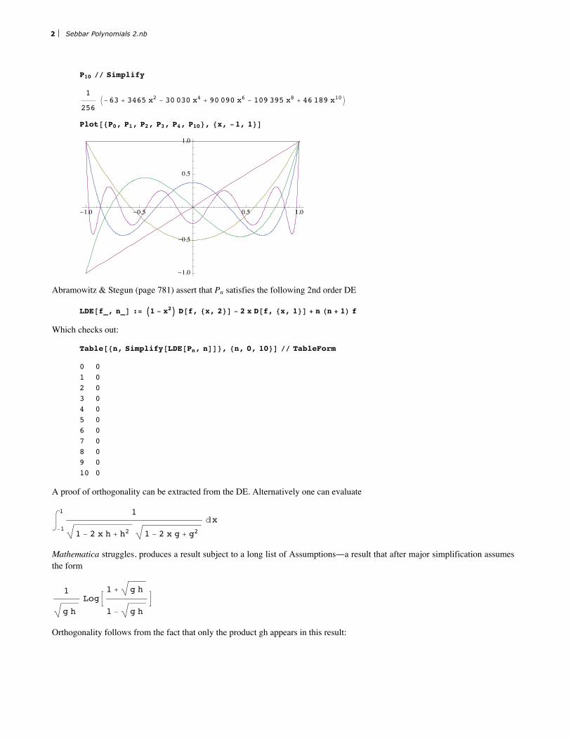
Plot@8P0, P1, P2, P3, P4, P10<, 8x, -1, 1<D
-1.0 -0.5 0.5 1.0
-1.0
-0.5
0.5
1.0
Abramowitz & Stegun (page 781) assert that Pn satisfies the following 2nd order DE
LDE@f_, n_D := I1 - x2M D@f, 8x, 2<D - 2 x D@f, 8x, 1<D + n Hn + 1L f
Which checks out:
Table@8n, Simplify@LDE@Pn, nDD<, 8n, 0, 10<D êê TableForm
0 01 02 03 04 05 06 07 08 09 010 0
A proof of orthogonality can be extracted from the DE. Alternatively one can evaluate
‡-1
1 1
1 - 2 x h + h2 1 - 2 x g + g2„x
Mathematica struggles, produces a result subject to a long list of Assumptions~a result that after major simplification assumesthe form
1
g hLogB
1 + g h
1 - g hF
Orthogonality follows from the fact that only the product gh appears in this result:
2 Sebbar Polynomials 2.nb

SeriesB1
kLogB
1 + k
1 - kF, 8k, 0, 10<F êê Normal
2 +2 k2
3+2 k4
5+2 k6
7+2 k8
9+2 k10
11
% ê. k Ø g h
2 +2 g h
3+2 g2 h2
5+2 g3 h3
7+2 g4 h4
9+2 g5 h5
11
We are led thus to the following inner product table:
TableBKroneckerDelta@m, nD2
2 n + 1, 8m, 0, 5<, 8n, 0, 5<F êê MatrixForm
2 0 0 0 0 0
0 2
30 0 0 0
0 0 2
50 0 0
0 0 0 2
70 0
0 0 0 0 2
90
0 0 0 0 0 2
11
ü Gegenbauer polynomials (ultraspherical polynomials of 0th order)
NOTE: These (as in A&S page 774) are usually denoted CnH0L, but I want to preserve Cn, so will denote them Gn.
The generating function is
-LogAR2E
-LogA1 + h2 - 2 h xE
GegenbauerSeries = SeriesA-LogA1 + h2 - 2 h xE, 8h, 0, 10<E;
Table@8n, Gn = SeriesCoefficient@GegenbauerSeries, nD<, 8n, 0, 10<D êê TableForm
0 01 2 x2 -1 + 2 x2
3 2
3I-3 x + 4 x3M
4 1
2I1 - 8 x2 + 8 x4M
5 2
5I5 x - 20 x3 + 16 x5M
6 1
3I-1 + 18 x2 - 48 x4 + 32 x6M
7 2
7I-7 x + 56 x3 - 112 x5 + 64 x7M
8 1
4I1 - 32 x2 + 160 x4 - 256 x6 + 128 x8M
9 2
9I9 x - 120 x3 + 432 x5 - 576 x7 + 256 x9M
10 1
5I-1 + 50 x2 - 400 x4 + 1120 x6 - 1280 x8 + 512 x10M
NOTE that G0 = 0, so the indices begin at n = 1.
Sebbar Polynomials 2.nb 3
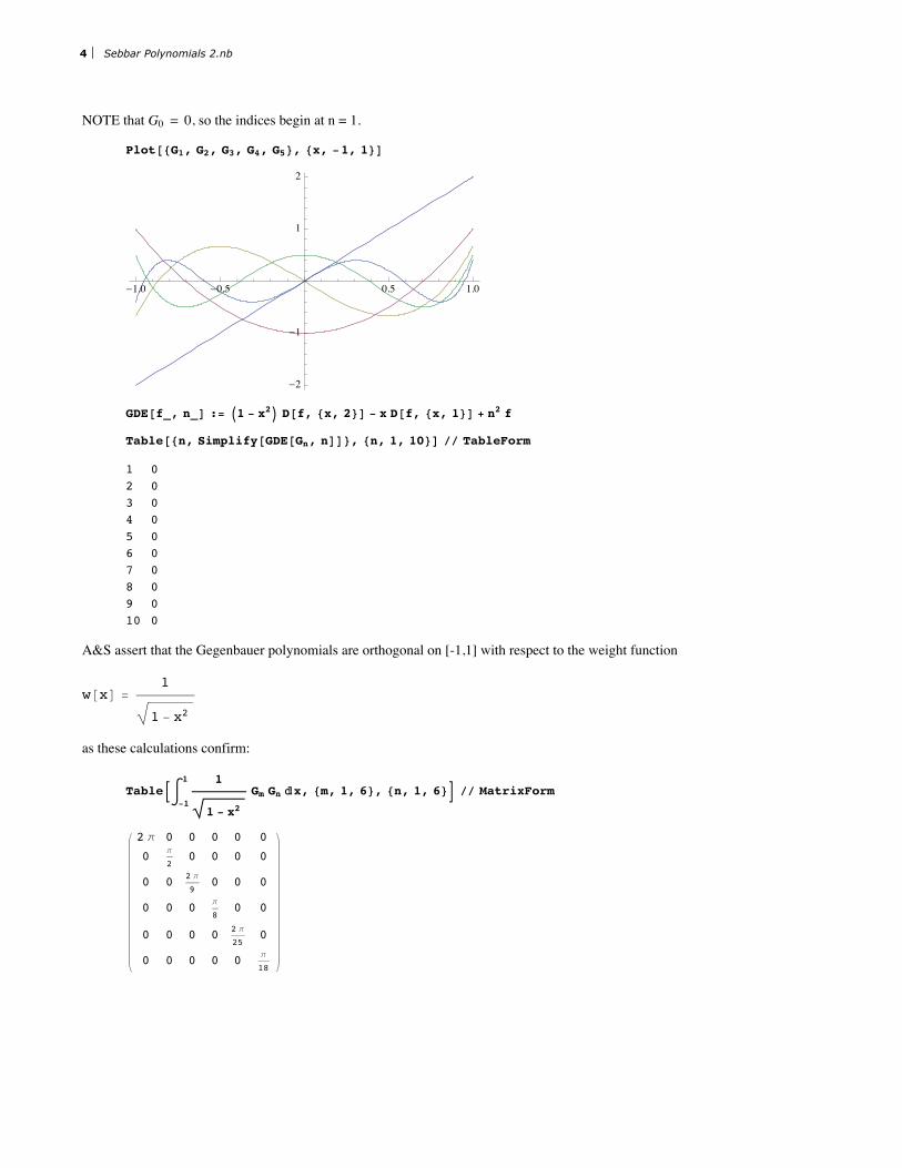
NOTE that G0 = 0, so the indices begin at n = 1.
Plot@8G1, G2, G3, G4, G5<, 8x, -1, 1<D
-1.0 -0.5 0.5 1.0
-2
-1
1
2
GDE@f_, n_D := I1 - x2M D@f, 8x, 2<D - x D@f, 8x, 1<D + n2 f
Table@8n, Simplify@GDE@Gn, nDD<, 8n, 1, 10<D êê TableForm
1 02 03 04 05 06 07 08 09 010 0
A&S assert that the Gegenbauer polynomials are orthogonal on [-1,1] with respect to the weight function
w@xD =1
1 - x2
as these calculations confirm:
TableB‡-1
1 1
1 - x2Gm Gn „x, 8m, 1, 6<, 8n, 1, 6<F êê MatrixForm
2 p 0 0 0 0 0
0 p
20 0 0 0
0 0 2 p
90 0 0
0 0 0 p
80 0
0 0 0 0 2 p
250
0 0 0 0 0 p
18
4 Sebbar Polynomials 2.nb

TableBKroneckerDelta@m, nD2 p
n2, 8m, 1, 6<, 8n, 1, 6<F êê MatrixForm
2 p 0 0 0 0 0
0 p
20 0 0 0
0 0 2 p
90 0 0
0 0 0 p
80 0
0 0 0 0 2 p
250
0 0 0 0 0 p
18
But Mathematica was unable in 30 minutes to say anything about the integral
‡-1
1 1
1 - x2LogA1 + h2 - 2 h xE LogA1 + g2 - 2 g xE „x
which in view of the preceding table we expect to have the value
‚k=1
¶ 2 p
k2ghk
2 p PolyLog@2, ghD
Which it might be interesting to check out numerically…but I won't.
ü Sabber polynomials
ü Polynomials of the 1st kind
The generating function is
In[201]:= S = I1 - 3 x h - h3M-n
Out[201]= I1 - h3 - 3 h xM-n
In[202]:= SabberSeries1 = Series@S, 8h, 0, 10<D;
In[203]:= Table@8n, n = SeriesCoefficient@SabberSeries1, nD<, 8n, 0, 5<D êê TableForm
Out[203]//TableForm=0 11 3 x n
2 9
2x2 n H1 + nL
3 n +9
2x3 H-2 - nL H-1 - nL n
4 -3 x H-1 - nL n -27
8x4 H-3 - nL H-2 - nL H-1 - nL n
5 9
2x2 H-2 - nL H-1 - nL n +
81
40x5 H-4 - nL H-3 - nL H-2 - nL H-1 - nL n
I extend the table (but don't print it):
Table@8n, n = SeriesCoefficient@SabberSeries1, nD<, 8n, 0, 10<D;
Sabber asserts that these are solutions of the following 3rd order DE:
Sebbar Polynomials 2.nb 5
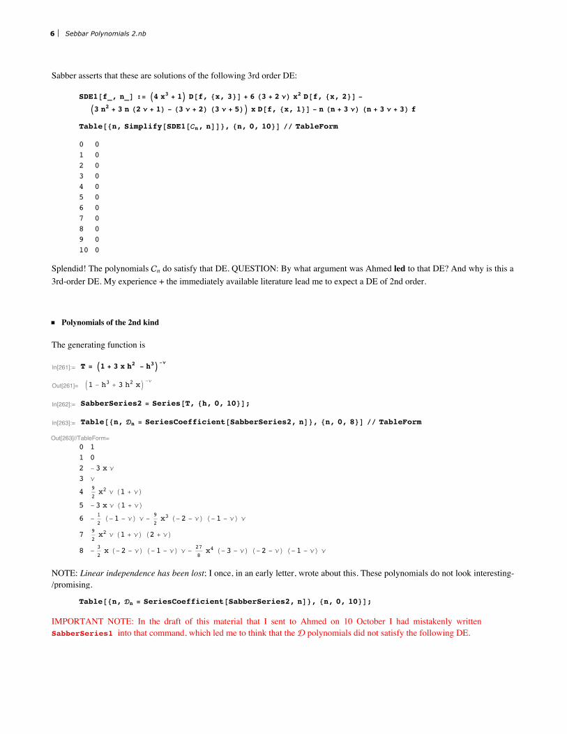
Sabber asserts that these are solutions of the following 3rd order DE:
SDE1@f_, n_D := I4 x3 + 1M D@f, 8x, 3<D + 6 H3 + 2 nL x2 D@f, 8x, 2<D -
I3 n2 + 3 n H2 n + 1L - H3 n + 2L H3 n + 5LM x D@f, 8x, 1<D - n Hn + 3 nL Hn + 3 n + 3L f
Table@8n, Simplify@SDE1@n, nDD<, 8n, 0, 10<D êê TableForm
0 01 02 03 04 05 06 07 08 09 010 0
Splendid! The polynomials n do satisfy that DE. QUESTION: By what argument was Ahmed led to that DE? And why is this a3rd-order DE. My experience + the immediately available literature lead me to expect a DE of 2nd order.
ü Polynomials of the 2nd kind
The generating function is
In[261]:= T = I1 + 3 x h2 - h3M-n
Out[261]= I1 - h3 + 3 h2 xM-n
In[262]:= SabberSeries2 = Series@T, 8h, 0, 10<D;
In[263]:= Table@8n, n = SeriesCoefficient@SabberSeries2, nD<, 8n, 0, 8<D êê TableForm
Out[263]//TableForm=0 11 02 -3 x n
3 n
4 9
2x2 n H1 + nL
5 -3 x n H1 + nL
6 -1
2H-1 - nL n -
9
2x3 H-2 - nL H-1 - nL n
7 9
2x2 n H1 + nL H2 + nL
8 -3
2x H-2 - nL H-1 - nL n -
27
8x4 H-3 - nL H-2 - nL H-1 - nL n
NOTE: Linear independence has been lost; I once, in an early letter, wrote about this. These polynomials do not look interesting-/promising.
Table@8n, n = SeriesCoefficient@SabberSeries2, nD<, 8n, 0, 10<D;
IMPORTANT NOTE: In the draft of this material that I sent to Ahmed on 10 October I had mistakenly writtenSabberSeries1 into that command, which led me to think that the polynomials did not satisfy the following DE.
ü Substitutional sense in which the DEs are siblings
6 Sebbar Polynomials 2.nb
ü
Substitutional sense in which the DEs are siblings
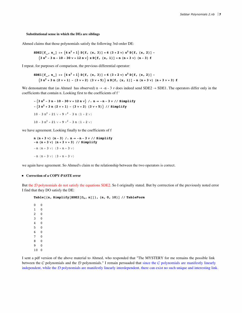
Ahmed claims that those polynomials satisfy the following 3rd-order DE:
SDE2@f_, n_D := I4 x3 + 1M D@f, 8x, 3<D + 6 H3 + 2 nL x2 D@f, 8x, 2<D -
I3 n2 - 3 n - 10 - 30 n + 12 n nM x D@f, 8x, 1<D + n Hn + 3 nL Hn - 3L f
I repeat, for purposes of comparison, the previous differential operator:
SDE1@f_, n_D := I4 x3 + 1M D@f, 8x, 3<D + 6 H3 + 2 nL x2 D@f, 8x, 2<D -
I3 n2 + 3 n H2 n + 1L - H3 n + 2L H3 n + 5LM x D@f, 8x, 1<D - n Hn + 3 nL Hn + 3 n + 3L f
We demonatrate that (as Ahmed has observed) n Ø -n - 3 n does indeed send SDE2 Ø SDE1. The operators differ only in thecoefficients that contain n. Looking first to the coefficients of f '
-I3 n2 - 3 n - 10 - 30 n + 12 n nM ê. n Ø -n - 3 n êê Simplify
-I3 n2 + 3 n H2 n + 1L - H3 n + 2L H3 n + 5LM êê Simplify
10 - 3 n2 + 21 n + 9 n2 - 3 n H1 + 2 nL
10 - 3 n2 + 21 n + 9 n2 - 3 n H1 + 2 nL
we have agreement. Looking finally to the coefficients of f
n Hn + 3 nL Hn - 3L ê. n Ø -n - 3 n êê Simplify-n Hn + 3 nL Hn + 3 n + 3L êê Simplify
-n Hn + 3 nL H3 + n + 3 nL
-n Hn + 3 nL H3 + n + 3 nL
we again have agreement. So Ahmed's claim re the relationship between the two operators is correct.
ü Correction of a COPY-PASTE error
But the polynomials do not satisfy the equations SDE2. So I originally stated. But by corrrection of the previously noted errorI find that they DO satisfy the DE:
Table@8n, Simplify@SDE2@n, nDD<, 8n, 0, 10<D êê TableForm
0 01 02 03 04 05 06 07 08 09 010 0
I sent a pdf version of the above material to Ahmed, who responded that "The MYSTERY for me remains the possible linkbetween the polynomials and the polynomials." I remain persuaded that since the polynomials are manifestly linearlyindependent, while the polynomials are manifestly linearly interdependent, there can exist no such unique and interesting link.
NOTE: The following material was written after the original pdf was written and delivered to Ahmed.
Sebbar Polynomials 2.nb 7

NOTE: The following material was written after the original pdf was written and delivered to Ahmed.
ü A second pair of Sabber polynomials
These alternative polynomials stand to the original Sabber polynomials rather like the Gegenbauer polynomials stand to theLegendre polynomials.
ü Alternative polynomials of the 1st kind
The generating function
S = I1 - 3 x h - h3M-n
is replaced by
In[120]:= S2 = LogA1 - 3 x h - h3E
Out[120]= LogA1 - h3 - 3 h xE
from which the n-parameter has disappeared (has become an inconsequential factor).
In[121]:= AlternativeSabberSeries1 = Series@S2, 8h, 0, 10<D;
In[122]:= Table@8n, n = SeriesCoefficient@AlternativeSabberSeries1, nD<, 8n, 0, 10<D êê TableForm
Out[122]//TableForm=0 01 -3 x
2 -9 x2
2
3 -1 - 9 x3
4 -3 x -81 x4
4
5 -9 x2 - 243 x5
5
6 -1
2- 27 x3 - 243 x6
2
7 -3 x - 81 x4 - 2187 x7
7
8 -27 x2
2- 243 x5 - 6561 x8
8
9 -1
3- 54 x3 - 729 x6 - 2187 x9
10 -3 x -405 x4
2- 2187 x7 - 59 049 x10
10
Following Ahmed, we construct the differential operator
AltSDE1@f_, n_D :=I4 x3 + 1M D@f, 8x, 3<D + 18 x2 D@f, 8x, 2<D - I3 n2 + 3 n - 10M x D@f, 8x, 1<D - n2 Hn + 3L f
8 Sebbar Polynomials 2.nb
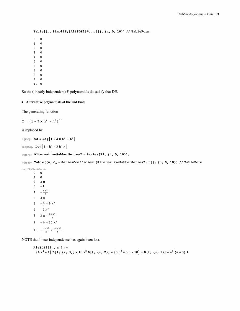
Table@8n, Simplify@AltSDE1@n, nDD<, 8n, 0, 10<D êê TableForm
0 01 02 03 04 05 06 07 08 09 010 0
So the (linearly independent) polynomials do satisfy that DE.
ü Alternative polynomials of the 2nd kind
The generating function
T = I1 + 3 x h2 - h3M-n
is replaced by
In[156]:= T2 = LogA1 + 3 x h2 - h3E
Out[156]= LogA1 - h3 + 3 h2 xE
In[157]:= AlternativeSabberSeries2 = Series@T2, 8h, 0, 10<D;
In[158]:= Table@8n, n = SeriesCoefficient@AlternativeSabberSeries2, nD<, 8n, 0, 10<D êê TableForm
Out[158]//TableForm=0 01 02 3 x3 -1
4 -9 x2
2
5 3 x
6 -1
2+ 9 x3
7 -9 x2
8 3 x -81 x4
4
9 -1
3+ 27 x3
10 -27 x2
2+
243 x5
5
NOTE that linear independence has again been lost.
AltSDE2@f_, n_D :=I4 x3 + 1M D@f, 8x, 3<D + 18 x2 D@f, 8x, 2<D - I3 n2 - 3 n - 10M x D@f, 8x, 1<D + n2 Hn - 3L f
Sebbar Polynomials 2.nb 9

Table@8n, Simplify@AltSDE2@n, nDD<, 8n, 0, 10<D êê TableForm
0 01 02 03 04 05 06 07 08 09 010 0
Again, the polynomials do satisfy the DE proposed by Ahmed.
ü Substitutional sense in which that alternate DEs are siblings
AltSDE2@f_, n_D :=I4 x3 + 1M D@f, 8x, 3<D + 18 x2 D@f, 8x, 2<D - I3 n2 - 3 n - 10M x D@f, 8x, 1<D + n2 Hn - 3L f
AltSDE1@f_, n_D :=I4 x3 + 1M D@f, 8x, 3<D + 18 x2 D@f, 8x, 2<D - I3 n2 + 3 n - 10M x D@f, 8x, 1<D - n2 Hn + 3L f
I3 n2 - 3 n - 10M ê. n Ø -n êê Simplify
SimplifyAI3 n2 + 3 n - 10ME
-10 + 3 n + 3 n2
-10 + 3 n + 3 n2
n2 Hn - 3L ê. n Ø -n êê SimplifySimplifyA-n2 Hn + 3LE
-n2 H3 + nL
-n2 H3 + nL
So n Ø -n sends AltSDE2 Ø AltSDE1.
ü General solutions of the Sebbar DEs
In the preceding discussion, patterns are most evident not in the polynomials but in the DEs that they satisfy. All four ofArmand's DEs are of the form
I4 x3 + 1M f'''@xD + a x2 f''@xD + b x f'@xD + c f@xD ã 0
In response to the command
DSolveAI4 x3 + 1M f'''@xD + a x2 f''@xD + b x f'@xD + c f@xD ã 0, f@xD, xE
Mathematica produces a result of the form
10 Sebbar Polynomials 2.nb
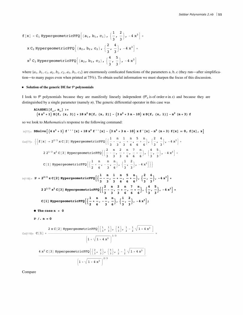
f@xD = C1 HypergeometricPFQB8a1, b1, c1<, :1
3,2
3>, -4 x3F +
x C2 HypergeometricPFQB8a2, b2, c2<, :2
3,4
3>, -4 x3F +
x2 C3 HypergeometricPFQB8a3, b3, c3<, :4
3,5
3>, -4 x3F
where 8a1, b1, c1, a2, b2, c2, a3, b3, c3} are enormously comlicated functions of the parameters a, b, c (they run~after simplifica-tion~to many pages even when printed at 75%). To obtain useful information we must sharpen the focus of this discussion.
ü Solution of the generic DE for polynomials
I look to polynomials because they are manifestly linearly independent Hn is of order n in x) and because they aredistinguished by a single parameter (namely ). The generic differential operator in this case was
AltSDE1@f_, n_D :=I4 x3 + 1M D@f, 8x, 3<D + 18 x2 D@f, 8x, 2<D - I3 n2 + 3 n - 10M x D@f, 8x, 1<D - n2 Hn + 3L f
so we look to Mathematica's response to the following command:
In[77]:= DSolveAI4 x3 + 1M f'''@xD + 18 x2 f''@xD - I3 n2 + 3 n - 10M x f'@xD - n2 Hn + 3L f@xD ã 0, f@xD, xE
Out[77]= ::f@xD Ø 22ê3 x C@2D HypergeometricPFQB:1
3-n
3,1
3+n
6,5
6+n
6>, :
2
3,4
3>, -4 x3F +
2 21ê3 x2 C@3D HypergeometricPFQB:2
3-n
3,2
3+n
6,7
6+n
6>, :
4
3,5
3>, -4 x3F +
C@1D HypergeometricPFQB:1
2+n
6, -
n
3,n
6>, :
1
3,2
3>, -4 x3F>>
In[118]:= = 22ê3 x C@2D HypergeometricPFQB:1
3-n
3,1
3+n
6,5
6+n
6>, :
2
3,4
3>, -4 x3F +
2 21ê3 x2 C@3D HypergeometricPFQB:2
3-n
3,2
3+n
6,7
6+n
6>, :
4
3,5
3>, -4 x3F +
C@1D HypergeometricPFQB:1
2+n
6, -
n
3,n
6>, :
1
3,2
3>, -4 x3F;
Ê The case n = 0
ê. n Ø 0
Out[119]= C@1D +2 x C@2D HypergeometricPFQB: 1
3, 1
3>, :
4
3>, 1
2-
1
21 + 4 x3 F
1 + 1 + 4 x31ê3
+
4 x2 C@3D HypergeometricPFQB: 2
3, 2
3>, :
5
3>, 1
2-
1
21 + 4 x3 F
1 + 1 + 4 x32ê3
Compare
Sebbar Polynomials 2.nb 11
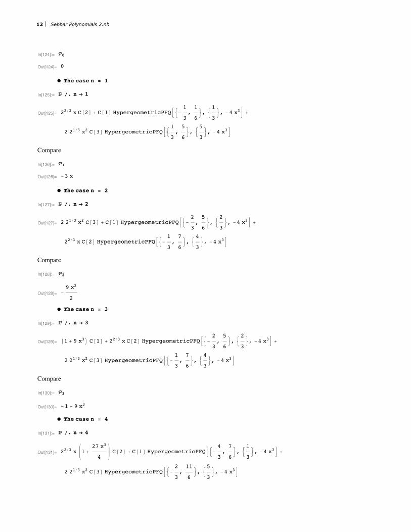
In[124]:= 0
Out[124]= 0
Ê The case n = 1
In[125]:= ê. n Ø 1
Out[125]= 22ê3 x C@2D + C@1D HypergeometricPFQB:-1
3,1
6>, :
1
3>, -4 x3F +
2 21ê3 x2 C@3D HypergeometricPFQB:1
3,5
6>, :
5
3>, -4 x3F
Compare
In[126]:= 1
Out[126]= -3 x
Ê The case n = 2
In[127]:= ê. n Ø 2
Out[127]= 2 21ê3 x2 C@3D + C@1D HypergeometricPFQB:-2
3,5
6>, :
2
3>, -4 x3F +
22ê3 x C@2D HypergeometricPFQB:-1
3,7
6>, :
4
3>, -4 x3F
Compare
In[128]:= 2
Out[128]= -9 x2
2
Ê The case n = 3
In[129]:= ê. n Ø 3
Out[129]= I1 + 9 x3M C@1D + 22ê3 x C@2D HypergeometricPFQB:-2
3,5
6>, :
2
3>, -4 x3F +
2 21ê3 x2 C@3D HypergeometricPFQB:-1
3,7
6>, :
4
3>, -4 x3F
Compare
In[130]:= 3
Out[130]= -1 - 9 x3
Ê The case n = 4
In[131]:= ê. n Ø 4
Out[131]= 22ê3 x 1 +27 x3
4C@2D + C@1D HypergeometricPFQB:-
4
3,7
6>, :
1
3>, -4 x3F +
2 21ê3 x2 C@3D HypergeometricPFQB:-2
3,11
6>, :
5
3>, -4 x3F
12 Sebbar Polynomials 2.nb

In[135]:= TogetherBx 1 +27 x3
4F
Out[135]=1
4x I4 + 27 x3M
Compare
In[133]:= 4 êê Simplify
Out[133]= -3
4x I4 + 27 x3M
Ê The case n = 5
In[136]:= ê. n Ø 5
Out[136]= 2 21ê3 x2 1 +27 x3
5C@3D + C@1D HypergeometricPFQB:-
5
3,5
6,4
3>, :
1
3,2
3>, -4 x3F +
22ê3 x C@2D HypergeometricPFQB:-4
3,7
6,5
3>, :
2
3,4
3>, -4 x3F
In[139]:= TogetherB x2 1 +27 x3
5F
Out[139]=1
5x2 I5 + 27 x3M
Compare
In[138]:= 5 êê Simplify
Out[138]= -9
5x2 I5 + 27 x3M
Ê The case n = 6
In[140]:= ê. n Ø 6
Out[140]= I1 + 54 x3 + 243 x6M C@1D + 22ê3 x C@2D HypergeometricPFQB:-5
3,11
6>, :
2
3>, -4 x3F +
2 21ê3 x2 C@3D HypergeometricPFQB:-4
3,13
6>, :
4
3>, -4 x3F
Compare
In[142]:= 6 êê Together
Out[142]=1
2I-1 - 54 x3 - 243 x6M
So it goes. We see that whenever n is a natural number the general solution of the generic DE assumes the form
HconstantL m + Hypergeometric + Hypergeometric
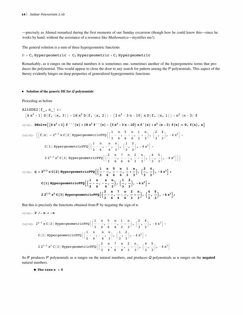
~precisely as Ahmed remarked during the first moments of our Sunday excursion (though how he could know this~since heworks by hand, without the assistance of a resource like Mathematica~mystifies me!).
The general solution is a sum of three hypergeometric functions
Sebbar Polynomials 2.nb 13
~precisely as Ahmed remarked during the first moments of our Sunday excursion (though how he could know this~since heworks by hand, without the assistance of a resource like Mathematica~mystifies me!).
The general solution is a sum of three hypergeometric functions
= C1 Hypergeometric + C2 Hypergeometric + C3 Hypergeometric
Remarkably, as n ranges on the natural numbers it is sometimes one, sometimes another of the hypergometric terms that pro-duces the polynomial. This would appear to close the door to any search for pattern among the polynomials. This aspect of thetheory evidently hinges on deep properties of generalized hypergeometric functions.
ü Solution of the generic DE for polynomials
Proceding as before
AltSDE2@f_, n_D :=
I4 x3 + 1M D@f, 8x, 3<D + 18 x2 D@f, 8x, 2<D - I3 n2 - 3 n - 10M x D@f, 8x, 1<D + n2 Hn - 3L f
In[145]:= DSolveAI4 x3 + 1M f'''@xD + 18 x2 f''@xD - I3 n2 - 3 n - 10M x f'@xD + n2 Hn - 3L f@xD ã 0, f@xD, xE
Out[145]= ::f@xD Ø 22ê3 x C@2D HypergeometricPFQB:1
3-n
6,5
6-n
6,1
3+n
3>, :
2
3,4
3>, -4 x3F +
C@1D HypergeometricPFQB:1
2-n
6, -
n
6,n
3>, :
1
3,2
3>, -4 x3F +
2 21ê3 x2 C@3D HypergeometricPFQB:2
3-n
6,7
6-n
6,2
3+n
3>, :
4
3,5
3>, -4 x3F>>
In[148]:= = 22ê3 x C@2D HypergeometricPFQB:1
3-n
6,5
6-n
6,1
3+n
3>, :
2
3,4
3>, -4 x3F +
C@1D HypergeometricPFQB:1
2-n
6, -
n
6,n
3>, :
1
3,2
3>, -4 x3F +
2 21ê3 x2 C@3D HypergeometricPFQB:2
3-n
6,7
6-n
6,2
3+n
3>, :
4
3,5
3>, -4 x3F;
But this is precisely the functions obtained from by negating the sign of n:
In[146]:= ê. n Ø -n
Out[146]= 22ê3 x C@2D HypergeometricPFQB:1
3-n
6,5
6-n
6,1
3+n
3>, :
2
3,4
3>, -4 x3F +
C@1D HypergeometricPFQB:1
2-n
6, -
n
6,n
3>, :
1
3,2
3>, -4 x3F +
2 21ê3 x2 C@3D HypergeometricPFQB:2
3-n
6,7
6-n
6,2
3+n
3>, :
4
3,5
3>, -4 x3F
So produces polynomials as n ranges on the natural numbers, and produces polynomials as n ranges on the negatednatural numbers.
Ê The case n = 0
14 Sebbar Polynomials 2.nb

In[159]:= ê. n Ø 00
Out[159]= C@1D +2 x C@2D HypergeometricPFQB: 1
3, 1
3>, :
4
3>, 1
2-
1
21 + 4 x3 F
1 + 1 + 4 x31ê3
+
4 x2 C@3D HypergeometricPFQB: 2
3, 2
3>, :
5
3>, 1
2-
1
21 + 4 x3 F
1 + 1 + 4 x32ê3
Out[160]= 0
Ê The case n = 1
In[195]:= ê. n Ø 1 ê. n Ø -11
Out[195]= C@1D HypergeometricPFQB:-1
6,1
3>, :
2
3>, -4 x3F +
22ê3 x C@2D HypergeometricPFQB:1
6,2
3>, :
4
3>, -4 x3F +
2 21ê3 x2 C@3D HypergeometricPFQB:1
2, 1, 1>, :
4
3,5
3>, -4 x3F
Out[196]= C@1D HypergeometricPFQB:-1
6,1
3>, :
2
3>, -4 x3F +
22ê3 x C@2D HypergeometricPFQB:1
6,2
3>, :
4
3>, -4 x3F +
2 21ê3 x2 C@3D HypergeometricPFQB:1
2, 1, 1>, :
4
3,5
3>, -4 x3F
Out[197]= 0
NOTE: This case appears to be exceptional. It is not obvious that constants C[i] (i = 1, 2, 3) can be found that from that series ofhypergeometric functions reproduces the 0-polynomial.
Ê The case n = 2
Sebbar Polynomials 2.nb 15

In[177]:= ê. n Ø 2 ê. n Ø -22
Out[177]= 22ê3 x C@2D + C@1D HypergeometricPFQB:-1
3,1
6>, :
1
3>, -4 x3F +
2 21ê3 x2 C@3D HypergeometricPFQB:1
3,5
6>, :
5
3>, -4 x3F
Out[178]= 22ê3 x C@2D + C@1D HypergeometricPFQB:-1
3,1
6>, :
1
3>, -4 x3F +
2 21ê3 x2 C@3D HypergeometricPFQB:1
3,5
6>, :
5
3>, -4 x3F
Out[179]= 3 x
Ê The case n = 3
In[180]:= ê. n Ø 3 ê. n Ø -33
Out[180]= C@1D + 22ê3 x C@2D HypergeometricPFQB:-1
6,1
3>, :
2
3>, -4 x3F +
2 21ê3 x2 C@3D HypergeometricPFQB:1
6,2
3>, :
4
3>, -4 x3F
Out[181]= C@1D + 22ê3 x C@2D HypergeometricPFQB:-1
6,1
3>, :
2
3>, -4 x3F +
2 21ê3 x2 C@3D HypergeometricPFQB:1
6,2
3>, :
4
3>, -4 x3F
Out[182]= -1
Ê The case n = 4
In[183]:= ê. n Ø 4 ê. n Ø -44
Out[183]= 2 21ê3 x2 C@3D + C@1D HypergeometricPFQB:-2
3, -
1
6,4
3>, :
1
3,2
3>, -4 x3F +
22ê3 x C@2D HypergeometricPFQB:-1
3,1
6,5
3>, :
2
3,4
3>, -4 x3F
Out[184]= 2 21ê3 x2 C@3D + C@1D HypergeometricPFQB:-2
3, -
1
6,4
3>, :
1
3,2
3>, -4 x3F +
22ê3 x C@2D HypergeometricPFQB:-1
3,1
6,5
3>, :
2
3,4
3>, -4 x3F
Out[185]= -9 x2
2
Ê The case n = 5
16 Sebbar Polynomials 2.nb
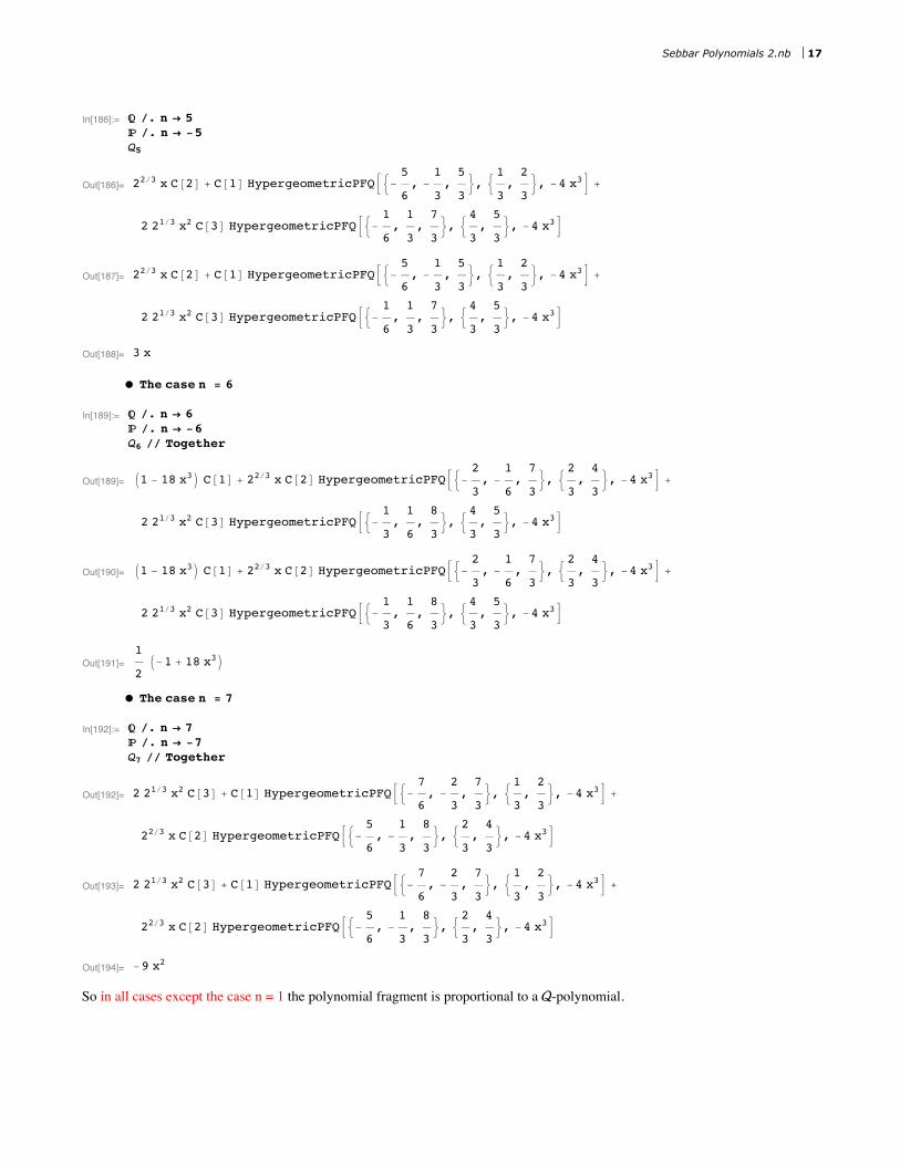
In[186]:= ê. n Ø 5 ê. n Ø -55
Out[186]= 22ê3 x C@2D + C@1D HypergeometricPFQB:-5
6, -
1
3,5
3>, :
1
3,2
3>, -4 x3F +
2 21ê3 x2 C@3D HypergeometricPFQB:-1
6,1
3,7
3>, :
4
3,5
3>, -4 x3F
Out[187]= 22ê3 x C@2D + C@1D HypergeometricPFQB:-5
6, -
1
3,5
3>, :
1
3,2
3>, -4 x3F +
2 21ê3 x2 C@3D HypergeometricPFQB:-1
6,1
3,7
3>, :
4
3,5
3>, -4 x3F
Out[188]= 3 x
Ê The case n = 6
In[189]:= ê. n Ø 6 ê. n Ø -66 êê Together
Out[189]= I1 - 18 x3M C@1D + 22ê3 x C@2D HypergeometricPFQB:-2
3, -
1
6,7
3>, :
2
3,4
3>, -4 x3F +
2 21ê3 x2 C@3D HypergeometricPFQB:-1
3,1
6,8
3>, :
4
3,5
3>, -4 x3F
Out[190]= I1 - 18 x3M C@1D + 22ê3 x C@2D HypergeometricPFQB:-2
3, -
1
6,7
3>, :
2
3,4
3>, -4 x3F +
2 21ê3 x2 C@3D HypergeometricPFQB:-1
3,1
6,8
3>, :
4
3,5
3>, -4 x3F
Out[191]=1
2I-1 + 18 x3M
Ê The case n = 7
In[192]:= ê. n Ø 7 ê. n Ø -77 êê Together
Out[192]= 2 21ê3 x2 C@3D + C@1D HypergeometricPFQB:-7
6, -
2
3,7
3>, :
1
3,2
3>, -4 x3F +
22ê3 x C@2D HypergeometricPFQB:-5
6, -
1
3,8
3>, :
2
3,4
3>, -4 x3F
Out[193]= 2 21ê3 x2 C@3D + C@1D HypergeometricPFQB:-7
6, -
2
3,7
3>, :
1
3,2
3>, -4 x3F +
22ê3 x C@2D HypergeometricPFQB:-5
6, -
1
3,8
3>, :
2
3,4
3>, -4 x3F
Out[194]= -9 x2
So in all cases except the case n = 1 the polynomial fragment is proportional to a -polynomial.
ü Solution of the generic DE for polynomials
Sebbar Polynomials 2.nb 17

ü
Solution of the generic DE for polynomials
Heere a second parameter n comes into play. Working from
In[240]:= SDE1@f_, n_D := I4 x3 + 1M D@f, 8x, 3<D + 6 H3 + 2 nL x2 D@f, 8x, 2<D -
I3 n2 + 3 n H2 n + 1L - H3 n + 2L H3 n + 5LM x D@f, 8x, 1<D - n Hn + 3 nL Hn + 3 n + 3L f
we command
In[198]:= DSolveAI4 x3 + 1M f'''@xD + 6 H3 + 2 nL x2 f''@xD -
I3 n2 + 3 n H2 n + 1L - H3 n + 2L H3 n + 5LM x f'@xD - n Hn + 3 nL Hn + 3 n + 3L f@xD ã 0, f@xD, xE
Out[198]= ::f@xD Ø 22ê3 x C@2D HypergeometricPFQB:1
3-n
3,1
3+n
6+
n
2,5
6+n
6+
n
2>, :
2
3,4
3>, -4 x3F +
2 21ê3 x2 C@3D HypergeometricPFQB:2
3-n
3,2
3+n
6+
n
2,7
6+n
6+
n
2>, :
4
3,5
3>, -4 x3F +
C@1D HypergeometricPFQB:-n
3,n
6+
n
2,1
2+n
6+
n
2>, :
1
3,2
3>, -4 x3F>>
and so have the generic solution
In[200]:= = 22ê3 x C@2D HypergeometricPFQB:1
3-n
3,1
3+n
6+
n
2,5
6+n
6+
n
2>, :
2
3,4
3>, -4 x3F +
2 21ê3 x2 C@3D HypergeometricPFQB:2
3-n
3,2
3+n
6+
n
2,7
6+n
6+
n
2>, :
4
3,5
3>, -4 x3F +
C@1D HypergeometricPFQB:-n
3,n
6+
n
2,1
2+n
6+
n
2>, :
1
3,2
3>, -4 x3F;
We let n march upward through the natural numbers, while leaving n unspecified:
Ê The case n = 0
In[204]:= ê. n Ø 00
Out[204]= C@1D + 22ê3 x C@2D HypergeometricPFQB:1
3,1
3+
n
2,5
6+
n
2>, :
2
3,4
3>, -4 x3F +
2 21ê3 x2 C@3D HypergeometricPFQB:2
3,2
3+
n
2,7
6+
n
2>, :
4
3,5
3>, -4 x3F
Out[205]= 1
Ê The case n = 1
In[206]:= ê. n Ø 11
Out[206]= 22ê3 x C@2D + C@1D HypergeometricPFQB:-1
3,1
6+
n
2,2
3+
n
2>, :
1
3,2
3>, -4 x3F +
2 21ê3 x2 C@3D HypergeometricPFQB:1
3,5
6+
n
2,4
3+
n
2>, :
4
3,5
3>, -4 x3F
Out[207]= 3 x n
Here the polynomial supplied by the general solution differs from 1by a factor, which can make no difference since the DE islinear:
18 Sebbar Polynomials 2.nb
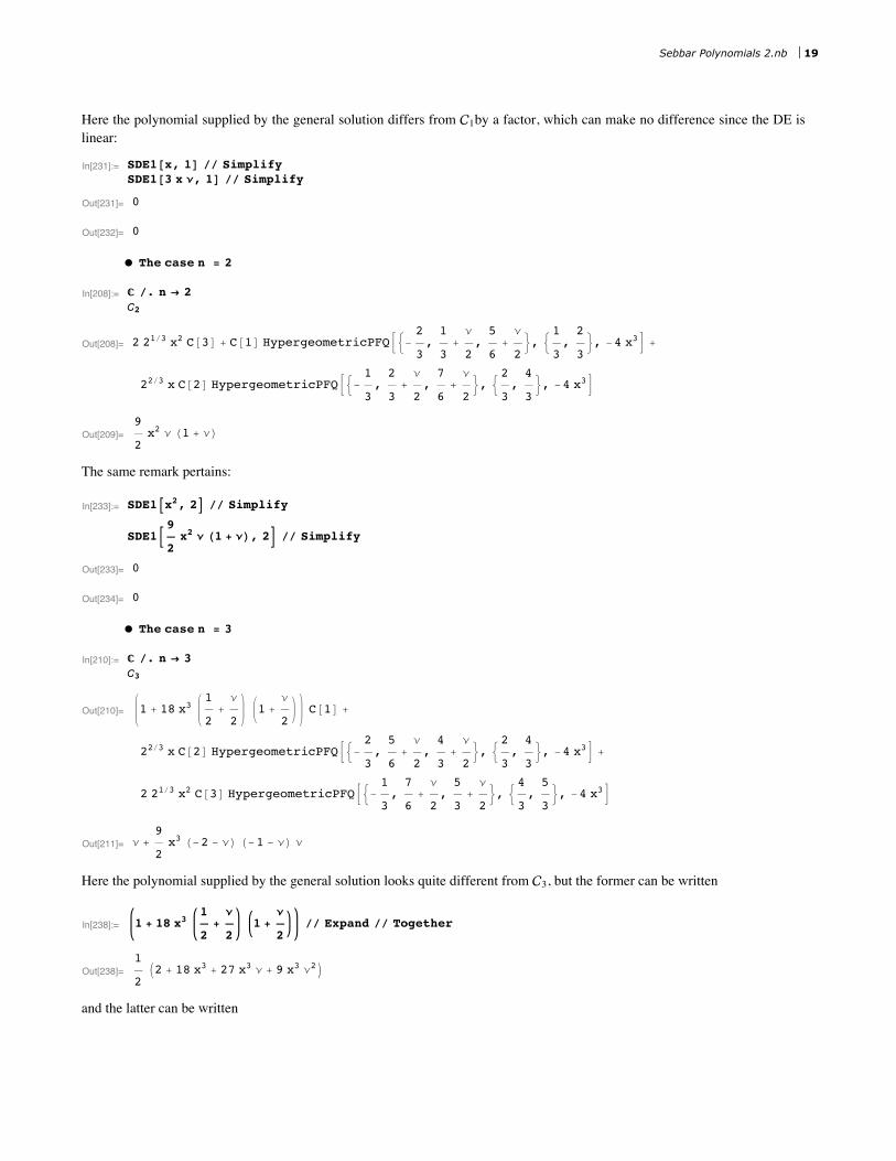
Here the polynomial supplied by the general solution differs from 1by a factor, which can make no difference since the DE islinear:
In[231]:= SDE1@x, 1D êê SimplifySDE1@3 x n, 1D êê Simplify
Out[231]= 0
Out[232]= 0
Ê The case n = 2
In[208]:= ê. n Ø 22
Out[208]= 2 21ê3 x2 C@3D + C@1D HypergeometricPFQB:-2
3,1
3+
n
2,5
6+
n
2>, :
1
3,2
3>, -4 x3F +
22ê3 x C@2D HypergeometricPFQB:-1
3,2
3+
n
2,7
6+
n
2>, :
2
3,4
3>, -4 x3F
Out[209]=9
2x2 n H1 + nL
The same remark pertains:
In[233]:= SDE1Ax2, 2E êê Simplify
SDE1B9
2x2 n H1 + nL, 2F êê Simplify
Out[233]= 0
Out[234]= 0
Ê The case n = 3
In[210]:= ê. n Ø 33
Out[210]= 1 + 18 x31
2+
n
21 +
n
2C@1D +
22ê3 x C@2D HypergeometricPFQB:-2
3,5
6+
n
2,4
3+
n
2>, :
2
3,4
3>, -4 x3F +
2 21ê3 x2 C@3D HypergeometricPFQB:-1
3,7
6+
n
2,5
3+
n
2>, :
4
3,5
3>, -4 x3F
Out[211]= n +9
2x3 H-2 - nL H-1 - nL n
Here the polynomial supplied by the general solution looks quite different from 3, but the former can be written
In[238]:= 1 + 18 x31
2+
n
21 +
n
2êê Expand êê Together
Out[238]=1
2I2 + 18 x3 + 27 x3 n + 9 x3 n2M
and the latter can be written
Sebbar Polynomials 2.nb 19
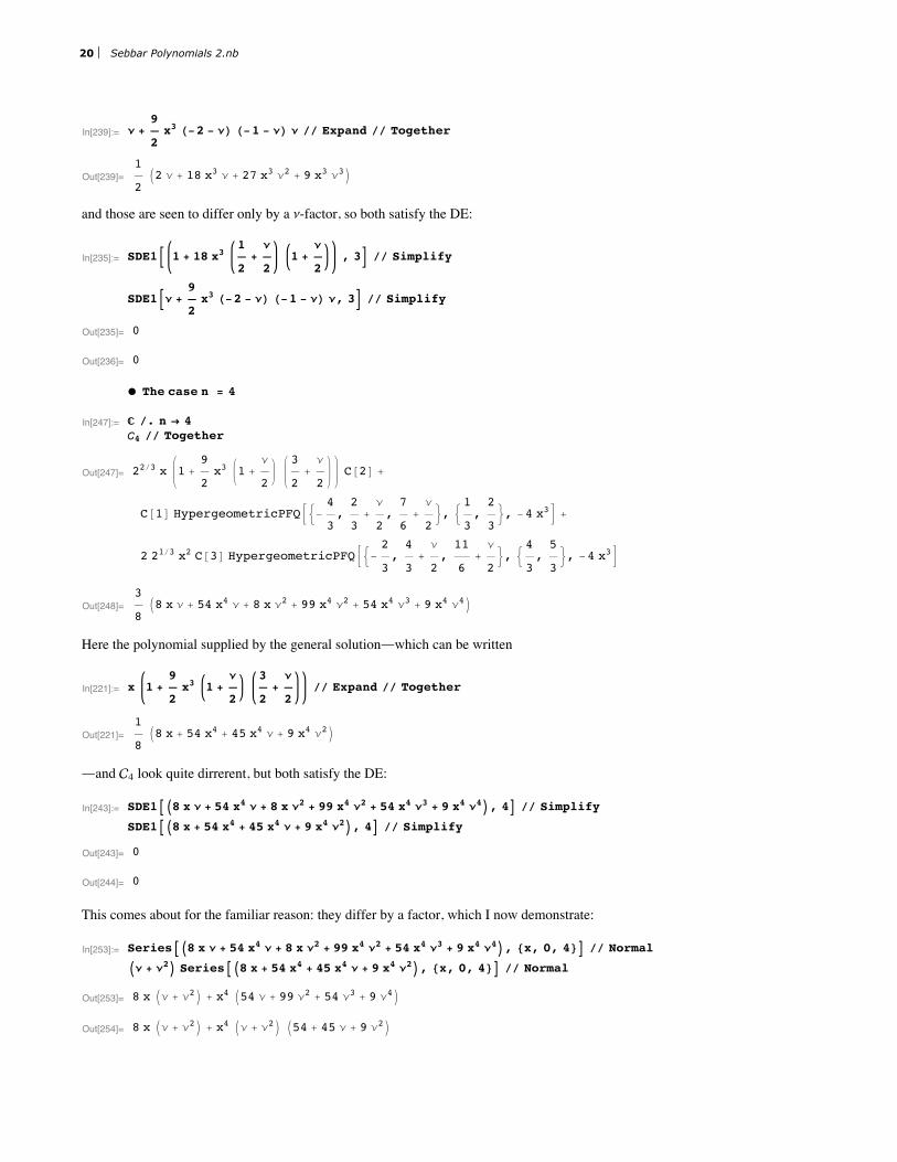
In[239]:= n +9
2x3 H-2 - nL H-1 - nL n êê Expand êê Together
Out[239]=1
2I2 n + 18 x3 n + 27 x3 n2 + 9 x3 n3M
and those are seen to differ only by a n-factor, so both satisfy the DE:
In[235]:= SDE1B 1 + 18 x31
2+
n
21 +
n
2, 3F êê Simplify
SDE1Bn +9
2x3 H-2 - nL H-1 - nL n, 3F êê Simplify
Out[235]= 0
Out[236]= 0
Ê The case n = 4
In[247]:= ê. n Ø 44 êê Together
Out[247]= 22ê3 x 1 +9
2x3 1 +
n
2
3
2+
n
2C@2D +
C@1D HypergeometricPFQB:-4
3,2
3+
n
2,7
6+
n
2>, :
1
3,2
3>, -4 x3F +
2 21ê3 x2 C@3D HypergeometricPFQB:-2
3,4
3+
n
2,11
6+
n
2>, :
4
3,5
3>, -4 x3F
Out[248]=3
8I8 x n + 54 x4 n + 8 x n2 + 99 x4 n2 + 54 x4 n3 + 9 x4 n4M
Here the polynomial supplied by the general solution~which can be written
In[221]:= x 1 +9
2x3 1 +
n
2
3
2+
n
2êê Expand êê Together
Out[221]=1
8I8 x + 54 x4 + 45 x4 n + 9 x4 n2M
~and 4 look quite dirrerent, but both satisfy the DE:
In[243]:= SDE1AI8 x n + 54 x4 n + 8 x n2 + 99 x4 n2 + 54 x4 n3 + 9 x4 n4M, 4E êê Simplify
SDE1AI8 x + 54 x4 + 45 x4 n + 9 x4 n2M, 4E êê Simplify
Out[243]= 0
Out[244]= 0
This comes about for the familiar reason: they differ by a factor, which I now demonstrate:
In[253]:= SeriesAI8 x n + 54 x4 n + 8 x n2 + 99 x4 n2 + 54 x4 n3 + 9 x4 n4M, 8x, 0, 4<E êê Normal
In + n2M SeriesAI8 x + 54 x4 + 45 x4 n + 9 x4 n2M, 8x, 0, 4<E êê Normal
Out[253]= 8 x In + n2M + x4 I54 n + 99 n2 + 54 n3 + 9 n4M
Out[254]= 8 x In + n2M + x4 In + n2M I54 + 45 n + 9 n2M
20 Sebbar Polynomials 2.nb
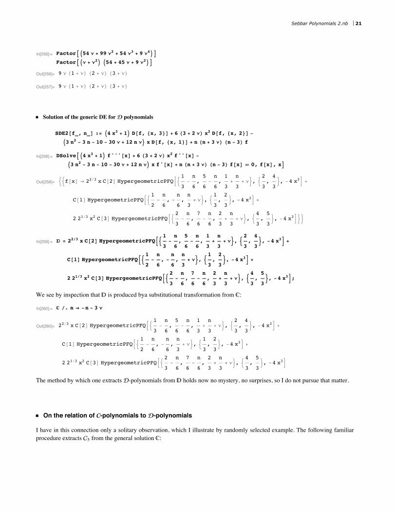
In[256]:= FactorAI54 n + 99 n2 + 54 n3 + 9 n4ME
FactorAIn + n2M I54 + 45 n + 9 n2ME
Out[256]= 9 n H1 + nL H2 + nL H3 + nL
Out[257]= 9 n H1 + nL H2 + nL H3 + nL
ü Solution of the generic DE for polynomials
SDE2@f_, n_D := I4 x3 + 1M D@f, 8x, 3<D + 6 H3 + 2 nL x2 D@f, 8x, 2<D -
I3 n2 - 3 n - 10 - 30 n + 12 n nM x D@f, 8x, 1<D + n Hn + 3 nL Hn - 3L f
In[258]:= DSolveAI4 x3 + 1M f'''@xD + 6 H3 + 2 nL x2 f''@xD -
I3 n2 - 3 n - 10 - 30 n + 12 n nM x f'@xD + n Hn + 3 nL Hn - 3L f@xD ã 0, f@xD, xE
Out[258]= ::f@xD Ø 22ê3 x C@2D HypergeometricPFQB:1
3-n
6,5
6-n
6,1
3+n
3+ n>, :
2
3,4
3>, -4 x3F +
C@1D HypergeometricPFQB:1
2-n
6, -
n
6,n
3+ n>, :
1
3,2
3>, -4 x3F +
2 21ê3 x2 C@3D HypergeometricPFQB:2
3-n
6,7
6-n
6,2
3+n
3+ n>, :
4
3,5
3>, -4 x3F>>
In[259]:= = 22ê3 x C@2D HypergeometricPFQB:1
3-n
6,5
6-n
6,1
3+n
3+ n>, :
2
3,4
3>, -4 x3F +
C@1D HypergeometricPFQB:1
2-n
6, -
n
6,n
3+ n>, :
1
3,2
3>, -4 x3F +
2 21ê3 x2 C@3D HypergeometricPFQB:2
3-n
6,7
6-n
6,2
3+n
3+ n>, :
4
3,5
3>, -4 x3F;
We see by inspection that is produced bya substitutional transformation from :
In[260]:= ê. n Ø -n - 3 n
Out[260]= 22ê3 x C@2D HypergeometricPFQB:1
3-n
6,5
6-n
6,1
3+n
3+ n>, :
2
3,4
3>, -4 x3F +
C@1D HypergeometricPFQB:1
2-n
6, -
n
6,n
3+ n>, :
1
3,2
3>, -4 x3F +
2 21ê3 x2 C@3D HypergeometricPFQB:2
3-n
6,7
6-n
6,2
3+n
3+ n>, :
4
3,5
3>, -4 x3F
The method by which one extracts -polynomials from holds now no mystery, no surprises, so I do not pursue that matter.
ü On the relation of -polynomials to -polynomials
I have in this connection only a solitary observation, which I illustrate by randomly selected example. The following familiarprocedure extracts 5 from the general solution :
Sebbar Polynomials 2.nb 21
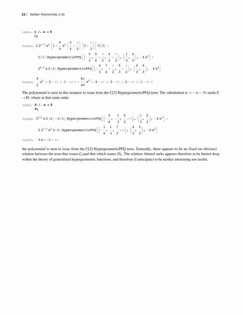
In[264]:= ê. n Ø 55
Out[264]= 2 21ê3 x2 1 +9
5x3
3
2+
n
22 +
n
2C@3D +
C@1D HypergeometricPFQB:-5
3,5
6+
n
2,4
3+
n
2>, :
1
3,2
3>, -4 x3F +
22ê3 x C@2D HypergeometricPFQB:-4
3,7
6+
n
2,5
3+
n
2>, :
2
3,4
3>, -4 x3F
Out[265]=9
2x2 H-2 - nL H-1 - nL n +
81
40x5 H-4 - nL H-3 - nL H-2 - nL H-1 - nL n
The polynomial is seen in this instance to issue from the C[3] HypergeometricPFQ term. The substitution n Ø -- n -- 3n sends Ø , where in that same order
In[266]:= ê. n Ø 55
Out[266]= 22ê3 x C@2D + C@1D HypergeometricPFQB:-5
6, -
1
3,5
3+ n>, :
1
3,2
3>, -4 x3F +
2 21ê3 x2 C@3D HypergeometricPFQB:-1
6,1
3,7
3+ n>, :
4
3,5
3>, -4 x3F
Out[267]= -3 x n H1 + nL
the polynomial is seen to issue from the C[2] HypergeometricPFQ term. Generally, there appears to be no fixed (or obvious)relation between the term that issues nand that which issues n. The relation Ahmed seeks appears therefore to be buried deepwithin the theory of generalized hypergeometric functions, and therefore (I anticipate) to be neither interesting nor useful.
22 Sebbar Polynomials 2.nb