Earth and Planetary Science Letters 379 (2013) 120–126

Contents lists available at ScienceDirect

Earth and Planetary Science Letters

www.elsevier.com/locate/epsl

Seasonal thermoelastic strain and postseismic effects in Parkfieldborehole dilatometers

Y. Ben-Zion ∗,1, A.A. Allam 2

Department of Earth Sciences, University of Southern California, Los Angeles, CA, 90089-0740, United States

a r t i c l e i n f o a b s t r a c t

Article history:Received 28 May 2013Received in revised form 5 August 2013Accepted 10 August 2013Available online xxxxEditor: Y. Ricard

Keywords:Parkfield borehole strainseasonal variationsthermoelastic straincrustal deformationthin surface layerstrain anomalies

Strainmeter records in three 176–323 m deep boreholes near Parkfield, CA, are dominated by seasonalfluctuations. We show that a significant part of the seasonal data may result from thermoelastic straininduced by atmospheric temperature variations. We test this hypothesis by computing thermoelasticstrain in an elastic half-space covered by a thin unconsolidated layer from atmospheric temperature andcomparing the results to the borehole strain records. The strain at depth is produced by the temperaturefield at the bottom of the unconsolidated layer. The model provides reasonable fits to the amplitudes andphases of the seasonal borehole signals. The two key model parameters, thickness of the unconsolidatedlayer (∼0.3–1.2 m at the used sites) and wavelength of the temperature field (3 km), are sufficientlyplausible to support the physical validity of the model. Two instances with persistent deviations betweenthe trends of the predicted thermoelastic strain and observed records may reflect shallow postseismiceffects of M � 4 nearby earthquakes.

© 2013 Elsevier B.V. All rights reserved.

1. Introduction

A wide variety of geophysical signals exhibit annual andsemi-annual seasonal variations with amplitudes, frequencies andphases that depend on the type of record and location. Exam-ples include geodetic data (e.g., Dong et al., 2002; Prawirodirdjoet al., 2006; Hill et al., 2009), water level changes (e.g., Ben-Zionet al., 1990; Manga, 1999), seismicity (e.g., Gao et al., 2000;Bettinelli et al., 2008; Hainzl et al., submitted for publication) andnoise in seismic waveforms (e.g. Stehly et al., 2006; Hillers andBen-Zion, 2011). Proposed mechanisms for these signals includerain and other hydrologic phenomena (e.g., Roeloffs, 2001; Hainzlet al., 2006; King et al., 2007), loadings due to changes in snow/icecover and atmospheric pressure (e.g. Christiansen et al., 2005;van Dam et al., 2010), ocean swells (e.g., Schulte-Pelkum et al.,2004; Kedar et al., 2008), thermoelastic strain (e.g., Berger, 1975;Ben-Zion and Leary, 1986) and other mechanisms listed in Donget al. (2002). Clarifying the dominant source or combination ofsources that is relevant in different circumstances is important forimproved understanding of crustal dynamics and design of removal

* Corresponding author.E-mail addresses: benzion@usc.edu (Y. Ben-Zion), aallam@usc.edu (A.A. Allam).

1 Tel.: +1 213 740 6734.2 Tel.: +1 213 740 6754.

0012-821X/$ – see front matter © 2013 Elsevier B.V. All rights reserved.http://dx.doi.org/10.1016/j.epsl.2013.08.024

filters for studies focusing on tectonic and other non-seasonal pro-cesses.

The Parkfield section of the San Andreas Fault is instrumentedwith borehole seismometers, dilatometers and strainmeters as partof a detailed monitoring effort (Bakun and Lindh, 1985). The re-sponse of Parkfield creepmeters to rain has been analyzed in detailby Roeloffs (2001). Examination of the results indicates that sig-nificant seasonal signals not explained by hydrologic effects ex-ist in some surface and borehole stations (E. Roeloffs, personalcomm., 2012). In this paper we analyze possible relations betweenatmospheric-induced thermoelastic strain and seasonal variationsin three Parkfield borehole dilatometers with depths >175 m. Weuse a model of strain generated by temporal variations of the at-mospheric temperature field, with a horizontal length scale relatedto topography, in an elastic half-space with a decoupled unconsol-idated (soil or gravel) upper layer (Ben-Zion and Leary, 1986). Themodel provides reasonable fits to the amplitudes and phases of theseasonal signals recorded at the borehole strainmeters. The resultsillustrate that thermoelastic strain generated by atmospheric tem-perature changes that travel through thin top soil layers can be animportant source of seasonal variations in borehole records. Therecognition that thermoelastic strain acts as a continuous drivingsource facilitates the identification of other sources of signals inthe observed data.

Y. Ben-Zion, A.A. Allam / Earth and Planetary Science Letters 379 (2013) 120–126 121

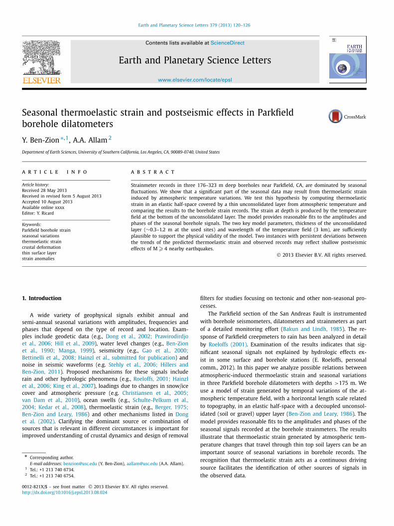
Fig. 1. Location map of the Parkfield area showing the three borehole dilatome-ter stations (blue triangles), the temperature, rainfall, and barometric pressure sites(orange triangle), two local seismic events that occurred during the time of inter-est (red stars), surface traces of the San Andreas Fault system (black lines), andother localities of interest (black circles). The background colors indicate topogra-phy with brown being high and green being low. The three borehole instrumentsare at depths of 204 m (VC), 323 m (FR), and 176 m (DL). The Mw 4.0 earthquakeoccurred at a depth of 12.73 km on February 26, 1999; the Mw 4.2 earthquake oc-curred at 9.44 km depth on November 12, 2002. These were the only two eventswith Mw > 3.5 to occur within 50 km of Parkfield from September 1996 to Septem-ber 2004. (For interpretation of the references to color in this figure legend, thereader is referred to the web version of this article.)

2. Analysis

2.1. Data

The locations of the three borehole strainmeter, atmospherictemperature, rainfall, and barometric pressure stations used in thisstudy are shown in Fig. 1. Strain records for 28 to 31 year periodsfrom the 3 borehole dilatometers were acquired from the USGS.The data were recorded on Sacks–Evertson dilatometers, whichmeasure the areal strain of the borehole cross-section, at depthsof 204 m (VC site), 323 m (FR site), and 176 m (DL site). Thesestations were selected because they have continuous long-termrecords. Station VC is located in a moderately cemented sandstone,FR is in a brecciated rhyolite, and DL is in a well-indurated sand-stone. The strain data were windowed from September 1996 toSeptember 2004 to avoid the exponential borehole relaxation inthe early records and the post-seismic effects of the September2004 Mw 6.0 Parkfield earthquake in the later part. A linear trendwas removed from the records and obvious offsets were correctedfollowing Agnew and Hodgkinson (2007). To facilitate a focus onseasonal variations, periods shorter than 30 days were removedusing a 4-pole butterworth filter.

We use a 31-year temperature record obtained from the NOAAData Center (http://www.ncdc.noaa.gov/cdo-web/). The tempera-ture was recorded at Coalinga about 15 km away from the near-est borehole dilatometer. Occasional data gaps, the largest ofwhich is 22 days, were linearly interpolated. The temperaturerecord was down-sampled to minimum and maximum daily val-ues and a cosine taper was applied to the data edges to re-duce the Gibbs effect in spectral analysis. There is little if anysnow in the study area which might decouple air and groundtemperatures. We also use a record of rainfall at Coalinga ob-tained from the NOAA Data Center, and barometric pressure record

at Gold Hill obtained from the USGS (http://earthquake.usgs.gov/monitoring/deformation/data/download/). We select data at thesestations (Fig. 1) as they are the most complete and noise-free avail-able in the region for the examined time period.

2.2. Model

The strain induced at depth by surface temperature changes iscalculated using the methodology of Ben-Zion and Leary (1986).The surface temperature field is assumed to be given approxi-mately by a standing wave of the form

T (x, y = 0, t) =∑ω

Tω cos(kx)ei(ωt−φ), (1)

where x is horizontal distance, y is depth, ω is the angular fre-quency, Tω = √

A2ω + B2

ω with Aω and Bω denoting amplitudes ofthe sine and cosine components of the temporal spectral decom-position, φ = tan−1(Aω/Bω), and k = 2π/λ is the wavenumber ofthe standing temperature field with wavelength λ. The latter wasshown in previous works to correlate with the local topography(Ben-Zion and Leary, 1986; Prawirodirdjo et al., 2006). A more gen-eral decomposition can incorporate a sum also over k to accountfor an arbitrary spatial temperature field. The spectral values of ωand φ are determined from observed temporal variations of atmo-spheric temperature at Coalinga.

Using (1) as a surface boundary condition, the horizontal ther-moelastic strain component εxx in a homogeneous elastic half-space can be written from the solution of Berger (1975) as

εxx =∑ω

(1 + σ

1 − σ

)(k

γ + k

)

·{[

2(1 − σ) + k

γ − k− ky

]e−ky − k

γ − ke−γ y

}

· [βTω cos(kx)ei(ωt−φ)], (2)

where γ = k[1 + iω/κk2]1/2 with Re(γ ) > 0, κ is the thermal dif-fusivity coefficient, β is the coefficient of linear thermal expansion,and σ is Poisson’s ratio. The term in (2) falling off with depth ase− Re(γ )y is the strain caused by temperature variations at a givendepth and is negligible below the thermal boundary layers associ-ated with different values of ω and k. However, the term falling ase−ky corresponds to strain transmitted from all shallower depthsthat are elastically coupled to the point under consideration andcan be significant to depths on the order of the surface tempera-ture wavelength.

Observed strain signals are characterized by amplitude andshape associated with the recorded frequencies and phases. Theamplitude depends on the source temperature field, several elasticand thermal parameters, and various additional 3D effects (to-pography, heterogeneities, etc.). As example, assuming in (2) anannual temperature change of 20 ◦C with a spatial wavelength of10 km, and using as in Ben-Zion and Leary (1986) β = 10−5 ◦C−1,κ = 6.09 · 10−2 m2/day and σ = 0.3, gives εxx = 2.7 · 10−7 at0.5 km depth, εxx = 1.3 · 10−7 at 1 km and εxx = 3.0 · 10−8 at3 km depth. With a shear modulus of 30 GPa, these strain val-ues correspond to ∼21.1 kPa at 0.5 km, ∼10.7 kPa at 1 km and∼2.4 kPa at 3 km. Similar parameter values and a surface tem-perature wavelength of 60 km lead to an average stress amplitudeover the depth range 1–10 km of ∼3.1 kPa. For comparison, Hainzlet al. (2006) estimated seasonal pore fluid pressure changes in thehighly-rainy Mt. Hochstaufen in Germany to be ∼1.3 kPa at 4 km.Bettinelli et al. (2008) estimated the crustal stresses associatedwith surface load changes due to summer monsoon rains in north-ern India to be 2–4 kPa. Gao et al. (2000) estimated an average

122 Y. Ben-Zion, A.A. Allam / Earth and Planetary Science Letters 379 (2013) 120–126

Fig. 2. Maximum amplitude of areal strain calculated at borehole depth 204 m (station VC) to illustrate trade-offs among model parameters λ (temperature field wavelength),σ (Poisson’s ratio), κ (thermal diffusivity) and yb (effective surface layer thickness). Non-uniqueness precludes a robust inversion for these parameters, but reasonableassumptions based on values for granitic rocks and previous works yield thermoelastic strain amplitudes which match the amplitudes of the observed borehole signals(Fig. 4).

stress of ∼2 kPa over the seismogenic zone due to seasonal atmo-spheric pressure variations in California. These amplitude estimatesindicate that seasonal thermoelastic strain can exert as strong aninfluence on crustal processes as other, more commonly studied,phenomena.

As the wavelength of the temperature field increases, the am-plitude of the thermoelastic strain at the surface decreases butthe strain also falls off more slowly with depth. A borehole

cross-section subjected to thermoelastic strain εxx (assumed herenormal to the topography) is expected to have, due to the Pois-son effect, a related εyy component, leading to an areal strainεA = εxx + εyy = (1 + σ)εxx . Fig. 2 shows estimated amplitudes ofareal strain, calculated from the observed temperature at Coalingaat depth of 204 m (station VC) for various combinations of wave-length of the temperature field, Poisson’s ratio, thermal diffusiv-ity, and surface layer thickness. As seen, plausible combinations

Y. Ben-Zion, A.A. Allam / Earth and Planetary Science Letters 379 (2013) 120–126 123

of parameters produce thermoelastic strain amplitudes larger than7.0 · 10−7 leading to stress amplitude larger than 55 kPa.

The shape of the strain signal (relative amplitudes and phasesof different frequency components) depends primarily on proper-ties of the effective operating source. Ben-Zion and Leary (1986)compared model results based on (2) with strainmeter data ob-served in a tunnel 10 m below the surface and found that theobserved record is delayed and has lower frequency content com-pared to the half-space model prediction. Prawirodirdjo et al.(2006) made similar observations in the context of three GPS ar-rays in southern California anchored to depth of about 10 m. Toaccount for the shape differences between the observed strainrecord and half-space model prediction, Ben-Zion and Leary (1986)added to the model an unconsolidated surface layer that is elasti-cally decoupled from the half-space. Since the temperature fieldhas to travel through the unconsolidated layer to induce strainin the solid below the layer, the thermoelastic strain in the un-derlying half-space is delayed, attenuated, and low-pass filteredcompared to predictions of the pure elastic half-space model.The thickness of the upper layer and dominant wavelength ofthe surface temperature field are the two key parameters of themodel.

2.3. Results

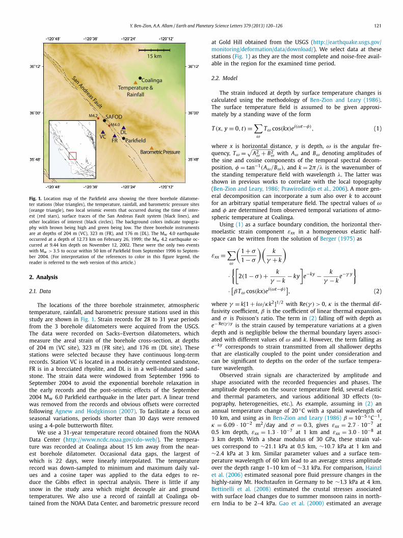
The Coalinga temperature record is first used in Eq. (2) tocalculate the half-space thermoelastic strain at a given boreholedepth. This is demonstrated in Fig. 3(a) for borehole station DL,assuming that the two temperature wavefield parameters are λ =3 km and location x = 0. The topography near Parkfield consistsof a series of ridges and valleys subparallel to the coastline, sothe strongest variation in elevation is in the fault-normal direc-tion. Topographic wavelengths affect the subsurface thermal fieldin relation to the depth of interest (e.g. Blackwell et al., 1980;Fulton et al., 2004). Since the instruments are at relatively shal-low depth, we use λ = 3 km which is representative of the localtopography.

Second, we measure the delay time between a given spectralcomponent of the model half-space strain and the observed straindata. The observed temperature record has several clear spectralpeaks with the dominant one at the annual period (Fig. 3(b)).The annual half-space strain should be delayed by about 45 daysfrom the corresponding surface temperature signal. An essen-tially zero further delay would indicate the lack of an unconsol-idated upper layer at that location (Ben-Zion and Leary, 1986;Tsai, 2011). Measuring the delay time �t between the annual (365days) components of the calculated half-space thermoelastic strainand observed strain data we obtain �t = 44 days for station DL(Fig. 3(b) inset). From �t , the effective thickness of the upper layeryb can be estimated (Ben-Zion and Leary, 1986) using

yb = 2�t√

πκ/τ , (3)

where τ is the period used in the calculation of the phase delay.For station DL with �t = 44 days and τ = 365 days, the obtainedvalue is yb = 1.19 m. Performing similar calculations for severalother periods with spectral peaks in the temperature record leadto similar values of delay time and corresponding yb thickness(Fig. 3(b)).

Third, the observed atmospheric temperature record is migratedto depth yb using Eq. (2) of Ben-Zion and Leary (1986) basedon heat conduction with (1) as the surface boundary condition(Fig. 3(c)). The temperature field at the bottom of the unconsoli-dated layer is used as the input for Eq. (2) to compute thermoelas-tic strain at the borehole instrument depth in a composite modelconsisting of a half-space covered by an unconsolidated layer of

Fig. 3. (a) Thermoelastic strain calculated (Eq. (2)) for station DL assuming a homo-geneous half-space (blue) and the low-pass filtered and detrended observed data(black). Extension is negative. Both curves have prominent seasonal variations butthe observed record is consistently delayed with respect to the predicted half-spacesignal. (b) Frequency spectrum of the temperature data at Coalinga. The annualperiod and two other marked peaks are used to calculate delay times and thick-nesses yb of the unconsolidated layer for station DL. The measured 44 days delayfor the annual period (inset) corresponds (Eq. (3)) to a layer thickness yb of 1.19 m.Results based on the other peaks lead to similar yb values. (c) The measured atmo-spheric temperature (green) used to compute the thermoelastic strain in a homo-geneous half-space shown in (a), and corresponding temperature signal migrated toyb = 1.19 m (red) used to calculate thermoelastic strain in the composite model.(For interpretation of the references to color in this figure legend, the reader is re-ferred to the web version of this article.)

thickness yb . The result is a time history of thermoelastic strainthat has been low-pass filtered, delayed, and attenuated comparedto the elastic half-space signal. The estimated yb values for stationsVC and FR are 0.28 m and 0.45 m, respectively. The thermoelastic

124 Y. Ben-Zion, A.A. Allam / Earth and Planetary Science Letters 379 (2013) 120–126

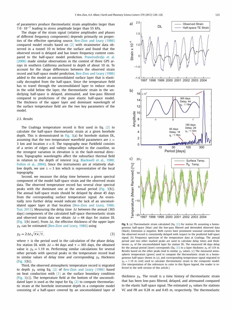
Fig. 4. Calculated thermoelastic strain in the composite model with an unconsolidated layer over a half-space (blue) and observed (black) borehole data for (a) the 204 mdeep station VC, (b) the 323 m deep station FR, and (c) the 176 m deep station DL. Extension is negative. Intervals longer than 1 month where the overall slopes of theobserved and predicted curves deviate are denoted with horizontal red bars (see text for additional explanation). The times of the two local Mw � 4.0 events shown inFig. 1 are marked with dotted red vertical lines. (d) Residual strain signals (data – synthetic) for station DL (purple), VC (blue) and FR (red), along with Coalinga rainfallrecord (bars at the bottom) and Gold Hill barometric pressure (black). The three residuals are correlated with each other and with the rain and barometric pressure data.(For interpretation of the references to color in this figure legend, the reader is referred to the web version of this article.)

strain signals predicted by the composite model for all 3 stationsfrom the atmospheric temperature data are shown together withthe observed strain records in Fig. 4.

As mentioned, the amplitude of the thermoelastic strain de-pends on the different elastic and thermal parameters in (2), alongwith the wavelength of the temperature field and the station po-sition in the field. Given the non-uniqueness involving signal am-plitude, even in our simple model, we simply select sets of rea-sonable parameters from those explored in Fig. 2 that demonstratethe physical plausibility of the model. Since the distances betweenstations is of the same order as the used λ = 3 km, we set for sim-plicity x = 0 at all stations and fold amplitude effects of somewhatdifferent λ and x values to material parameters. We obtain closefits to the observed amplitudes at the three sites with reasonablematerial properties. In all locations we use σ = 0.33 correspond-ing to damaged rock, half-space κ = 6.09 · 10−2 m2/day and soillayer diffusivity κ = 2.16 · 10−2 m2/day. For stations VC and FR onthe SW side of the fault we use β = 10−5 ◦C−1, while for stationDL on the NE side we increase this slightly to β = 1.2 · 10−5 ◦C−1.

During most of the examined period the general trend of theobserved data at each site follows closely the slope of the calcu-lated thermoelastic strain. Persistent deviations between the pre-dicted and observed signals suggest the existence of other sources(Ben-Zion et al., 1990). We quantitatively search for deviations oftrends between the two signals over time intervals larger than 30days (the smallest period in the examined data) as follows. First,

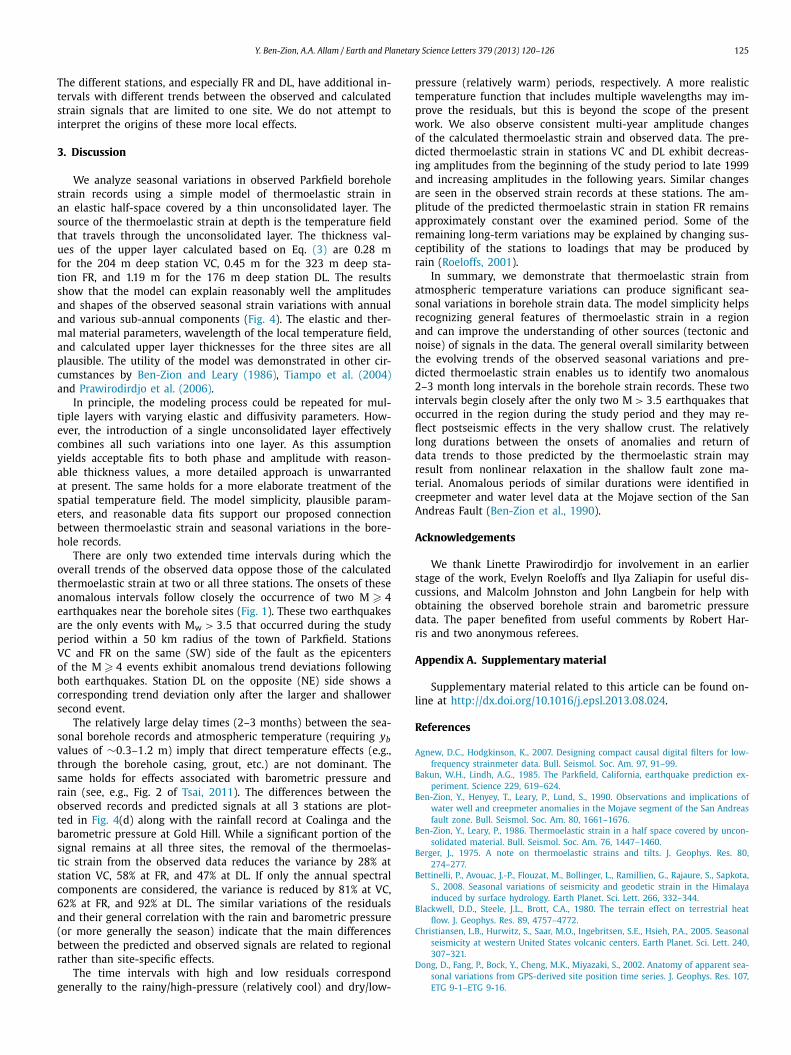
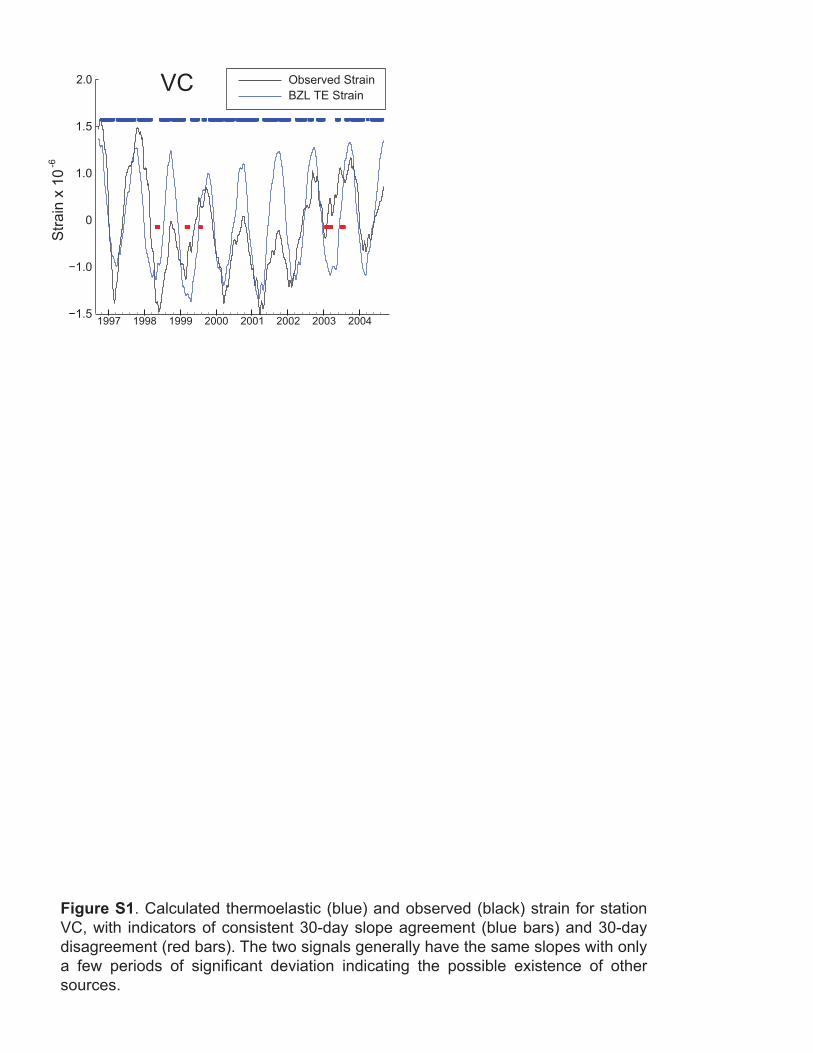
we calculate the slope at each point in the two signals. If the signsof slopes at a given time are the same we assign 1 to that point,and if they disagree we assign 0 to that point. Next, we examinea 30-day window around each point in the records. If the slopesare in agreement (all 1’s) or general disagreement (all 0’s) for theentire 30 days, we retain the values of 1 or 0 at that point. Ifthe slopes include during 30 days both agreement and disagree-ment, we remove the point from consideration. This procedureprovides a simple indication of time intervals when the trends ofthe observed and calculated signals consistently agree or consis-tently disagree for a minimum of 30 days (supplementary Fig. S1).

There are only three time intervals when the trends of thepredicted thermoelastic strain and borehole data have persistentdisagreements in at least two of the three stations (horizontal redbars in Fig. 4). Two of these instances begin shortly after the ori-gin times (dotted vertical red lines) of the two M � 4 earthquakesmarked in Fig. 1 and persist for about 2–3 months. Stations VC andFR on the SW side of the SAF have three common anomalous timeintervals (Figs. 4(a) and 4(b)): a period where the two signals aresomewhat out of phase around April 1998, and two periods imme-diately after the origin times of the two M � 4 earthquakes. StationDL on the NE side of the fault has one anomalous interval with op-posite overall trends between the observed and predicted signalsthat coincides with the second anomalous period at stations VCand FR (Fig. 4(c)). This second anomaly that is common to all 3 sta-tions is associated with the larger and shallower M 4.2 earthquake.

Y. Ben-Zion, A.A. Allam / Earth and Planetary Science Letters 379 (2013) 120–126 125

The different stations, and especially FR and DL, have additional in-tervals with different trends between the observed and calculatedstrain signals that are limited to one site. We do not attempt tointerpret the origins of these more local effects.

3. Discussion

We analyze seasonal variations in observed Parkfield boreholestrain records using a simple model of thermoelastic strain inan elastic half-space covered by a thin unconsolidated layer. Thesource of the thermoelastic strain at depth is the temperature fieldthat travels through the unconsolidated layer. The thickness val-ues of the upper layer calculated based on Eq. (3) are 0.28 mfor the 204 m deep station VC, 0.45 m for the 323 m deep sta-tion FR, and 1.19 m for the 176 m deep station DL. The resultsshow that the model can explain reasonably well the amplitudesand shapes of the observed seasonal strain variations with annualand various sub-annual components (Fig. 4). The elastic and ther-mal material parameters, wavelength of the local temperature field,and calculated upper layer thicknesses for the three sites are allplausible. The utility of the model was demonstrated in other cir-cumstances by Ben-Zion and Leary (1986), Tiampo et al. (2004)and Prawirodirdjo et al. (2006).

In principle, the modeling process could be repeated for mul-tiple layers with varying elastic and diffusivity parameters. How-ever, the introduction of a single unconsolidated layer effectivelycombines all such variations into one layer. As this assumptionyields acceptable fits to both phase and amplitude with reason-able thickness values, a more detailed approach is unwarrantedat present. The same holds for a more elaborate treatment of thespatial temperature field. The model simplicity, plausible param-eters, and reasonable data fits support our proposed connectionbetween thermoelastic strain and seasonal variations in the bore-hole records.

There are only two extended time intervals during which theoverall trends of the observed data oppose those of the calculatedthermoelastic strain at two or all three stations. The onsets of theseanomalous intervals follow closely the occurrence of two M � 4earthquakes near the borehole sites (Fig. 1). These two earthquakesare the only events with Mw > 3.5 that occurred during the studyperiod within a 50 km radius of the town of Parkfield. StationsVC and FR on the same (SW) side of the fault as the epicentersof the M � 4 events exhibit anomalous trend deviations followingboth earthquakes. Station DL on the opposite (NE) side shows acorresponding trend deviation only after the larger and shallowersecond event.

The relatively large delay times (2–3 months) between the sea-sonal borehole records and atmospheric temperature (requiring ybvalues of ∼0.3–1.2 m) imply that direct temperature effects (e.g.,through the borehole casing, grout, etc.) are not dominant. Thesame holds for effects associated with barometric pressure andrain (see, e.g., Fig. 2 of Tsai, 2011). The differences between theobserved records and predicted signals at all 3 stations are plot-ted in Fig. 4(d) along with the rainfall record at Coalinga and thebarometric pressure at Gold Hill. While a significant portion of thesignal remains at all three sites, the removal of the thermoelas-tic strain from the observed data reduces the variance by 28% atstation VC, 58% at FR, and 47% at DL. If only the annual spectralcomponents are considered, the variance is reduced by 81% at VC,62% at FR, and 92% at DL. The similar variations of the residualsand their general correlation with the rain and barometric pressure(or more generally the season) indicate that the main differencesbetween the predicted and observed signals are related to regionalrather than site-specific effects.

The time intervals with high and low residuals correspondgenerally to the rainy/high-pressure (relatively cool) and dry/low-

pressure (relatively warm) periods, respectively. A more realistictemperature function that includes multiple wavelengths may im-prove the residuals, but this is beyond the scope of the presentwork. We also observe consistent multi-year amplitude changesof the calculated thermoelastic strain and observed data. The pre-dicted thermoelastic strain in stations VC and DL exhibit decreas-ing amplitudes from the beginning of the study period to late 1999and increasing amplitudes in the following years. Similar changesare seen in the observed strain records at these stations. The am-plitude of the predicted thermoelastic strain in station FR remainsapproximately constant over the examined period. Some of theremaining long-term variations may be explained by changing sus-ceptibility of the stations to loadings that may be produced byrain (Roeloffs, 2001).

In summary, we demonstrate that thermoelastic strain fromatmospheric temperature variations can produce significant sea-sonal variations in borehole strain data. The model simplicity helpsrecognizing general features of thermoelastic strain in a regionand can improve the understanding of other sources (tectonic andnoise) of signals in the data. The general overall similarity betweenthe evolving trends of the observed seasonal variations and pre-dicted thermoelastic strain enables us to identify two anomalous2–3 month long intervals in the borehole strain records. These twointervals begin closely after the only two M > 3.5 earthquakes thatoccurred in the region during the study period and they may re-flect postseismic effects in the very shallow crust. The relativelylong durations between the onsets of anomalies and return ofdata trends to those predicted by the thermoelastic strain mayresult from nonlinear relaxation in the shallow fault zone ma-terial. Anomalous periods of similar durations were identified increepmeter and water level data at the Mojave section of the SanAndreas Fault (Ben-Zion et al., 1990).

Acknowledgements

We thank Linette Prawirodirdjo for involvement in an earlierstage of the work, Evelyn Roeloffs and Ilya Zaliapin for useful dis-cussions, and Malcolm Johnston and John Langbein for help withobtaining the observed borehole strain and barometric pressuredata. The paper benefited from useful comments by Robert Har-ris and two anonymous referees.

Appendix A. Supplementary material

Supplementary material related to this article can be found on-line at http://dx.doi.org/10.1016/j.epsl.2013.08.024.

References

Agnew, D.C., Hodgkinson, K., 2007. Designing compact causal digital filters for low-frequency strainmeter data. Bull. Seismol. Soc. Am. 97, 91–99.

Bakun, W.H., Lindh, A.G., 1985. The Parkfield, California, earthquake prediction ex-periment. Science 229, 619–624.

Ben-Zion, Y., Henyey, T., Leary, P., Lund, S., 1990. Observations and implications ofwater well and creepmeter anomalies in the Mojave segment of the San Andreasfault zone. Bull. Seismol. Soc. Am. 80, 1661–1676.

Ben-Zion, Y., Leary, P., 1986. Thermoelastic strain in a half space covered by uncon-solidated material. Bull. Seismol. Soc. Am. 76, 1447–1460.

Berger, J., 1975. A note on thermoelastic strains and tilts. J. Geophys. Res. 80,274–277.

Bettinelli, P., Avouac, J.-P., Flouzat, M., Bollinger, L., Ramillien, G., Rajaure, S., Sapkota,S., 2008. Seasonal variations of seismicity and geodetic strain in the Himalayainduced by surface hydrology. Earth Planet. Sci. Lett. 266, 332–344.

Blackwell, D.D., Steele, J.L., Brott, C.A., 1980. The terrain effect on terrestrial heatflow. J. Geophys. Res. 89, 4757–4772.

Christiansen, L.B., Hurwitz, S., Saar, M.O., Ingebritsen, S.E., Hsieh, P.A., 2005. Seasonalseismicity at western United States volcanic centers. Earth Planet. Sci. Lett. 240,307–321.

Dong, D., Fang, P., Bock, Y., Cheng, M.K., Miyazaki, S., 2002. Anatomy of apparent sea-sonal variations from GPS-derived site position time series. J. Geophys. Res. 107,ETG 9-1–ETG 9-16.

126 Y. Ben-Zion, A.A. Allam / Earth and Planetary Science Letters 379 (2013) 120–126

Fulton, P.M., Saffer, D.M., Harris, R.N., Bekins, B.A., 2004. Re-evaluation of heat flowdata near Parkfield, CA: Evidence for a weak San Andreas Fault. Geophys. Res.Lett. 31, L15S15, http://dx.doi.org/10.1029/2003GL019378.

Gao, S.S., Silver, P.G., Linde, S.T., Sacks, I.S., 2000. Annual modulation of triggeredseismicity following the 1992 Landers earthquake in California. Nature 406,500–505.

Hainzl, S., Ben-Zion, Y., Cattania, C., Wassermann, J., submitted for publication. Test-ing atmospheric and tidal earthquake triggering at Mt. Hochstaufen, Germany.J. Geophys. Res.

Hainzl, S., Kraft, T., Wassermann, J., Igel, H., Schmedes, E., 2006. Evidencefor rainfall-triggered earthquake activity. Geophys. Res. Lett. 33, L19303,http://dx.doi.org/10.1029/2006GL027642.

Hill, E.M., Davis, J.L., Elósegui, P., Wernicke, B.P., Malikowski, E., Niemi, N.A., 2009.Characterization of sitespecific GPS errors using a short-baseline network ofbraced monuments at Yucca Mountain, southern Nevada. J. Geophys. Res. 114,B11402, http://dx.doi.org/10.1029/2008JB006027.

Hillers, G., Ben-Zion, Y., 2011. Seasonal variations of observed noise amplitudes at2–18 Hz in southern California. Geophys. J. Int. 184, 860–868, http://dx.doi.org/10.1111/j.1365-246X.2010.04886.x.

Kedar, S., Longuet-Higgins, M., Webb, F., Graham, N., Clayton, R., Jones, C., 2008.The origin of deep ocean microseisms in the North Atlantic Ocean. Proc. R. Soc.A 464, 777–793, http://dx.doi.org/10.1098/rspa.2007.0277.

King, N.E., Argus, D., Langbein, J., Agnew, D.C., Bawden, G., Dollar, R.S., Liu, Z., Gal-loway, D., Reichard, E., Yong, A., Webb, F.H., Bock, Y., Stark, K., Barseghian, D.,

2007. Space geodetic observation of expansion of the San Gabriel Valley, Cali-fornia, aquifer system, during heavy rainfall in winter 2004–2005. J. Geophys.Res. 112.

Manga, M., 1999. On the timescales characterizing groundwater discharge at springs.J. Hydrol. 219, 56–69.

Prawirodirdjo, L., Ben-Zion, Y., Bock, Y., 2006. Observation and modeling of thermoe-lastic strain in SCIGN daily position time series. J. Geophys. Res. 111, B02408,http://dx.doi.org/10.1029/2005JB003716.

Roeloffs, E., 2001. Creep-rate changes at Parkfield, California 1966–1999: Seasonal,precipitation-induced, and tectonic. J. Geophys. Res. 106, 16525–16547.

Schulte-Pelkum, V., Earle, P.S., Vernon, F.L., 2004. Strong directivity of ocean-generated seismic noise. Geochem. Geophys. Geosyst. 5 (3), http://dx.doi.org/10.1029/2003GC000520.

Stehly, L., Campillo, M., Shapiro, N.M., 2006. A study of the seismic noise from itslong-range correlation properties. J. Geophys. Res. 111 (B10), B10306.

Tiampo, K.F., Rundle, J.B., Klein, W., Ben-Zion, Y., McGinnis, S., 2004. Using eigen-pattern analysis to constrain seasonal signals in Southern California. Pure Appl.Geophys. 161, 1991–2003.

Tsai, V.C., 2011. A model for seasonal changes in GPS positions and seismic wavespeeds due to thermoelastic and hydrologic variations. J. Geophys. Res. 116,B04404, http://dx.doi.org/10.1029/2010JB008156.

van Dam, T., Altamimi, Z., Collilieux, X., Ray, J., 2010. Topographically in-duced height errors in predicted atmospheric loading effects. J. Geophys.Res. 115.

1997 1998 1999 2000 2001 2002 2003 2004

VC Observed StrainBZL TE Strain

Stra

in x

10

-6

−1.5

−1.0

0

1.0

1.5

2.0

Figure S1. Calculated thermoelastic (blue) and observed (black) strain for station VC, with indicators of consistent 30-day slope agreement (blue bars) and 30-day disagreement (red bars). The two signals generally have the same slopes with only a few periods of significant deviation indicating the possible existence of other sources.