seasonal hydrologic prediction in the united states

Hydrol. Earth Syst. Sci., 15, 3529–3538, 2011www.hydrol-earth-syst-sci.net/15/3529/2011/doi:10.5194/hess-15-3529-2011© Author(s) 2011. CC Attribution 3.0 License.

Hydrology andEarth System

Sciences

Seasonal hydrologic prediction in the United States: understandingthe role of initial hydrologic conditions and seasonal climate forecastskill

S. Shukla and D. P. Lettenmaier

Department of Civil and Environmental Engineering, University of Washington, Seattle, 98195, USA

Received: 30 June 2011 – Published in Hydrol. Earth Syst. Sci. Discuss.: July 2011Revised: 23 October 2011 – Accepted: 3 November 2011 – Published: 22 November 2011

Abstract. Seasonal hydrologic forecasts derive their skillfrom knowledge of initial hydrologic conditions and climateforecast skill associated with seasonal climate outlooks. De-pending on the type of hydrological regime and the sea-son, the relative contributions of initial hydrologic condi-tions and climate forecast skill to seasonal hydrologic fore-cast skill vary. We seek to quantify these contributions ona relative basis across the Conterminous United States. Weconstructed two experiments – Ensemble Streamflow Predic-tion and reverse-Ensemble Streamflow Prediction – to par-tition the contributions of the initial hydrologic conditionsand climate forecast skill to overall forecast skill. In en-semble streamflow prediction (first experiment) hydrologicforecast skill is derived solely from knowledge of initial hy-drologic conditions, whereas in reverse-ensemble streamflowprediction (second experiment), it is derived solely from at-mospheric forcings (i.e. perfect climate forecast skill). Usingthe ratios of root mean square error in predicting cumulativerunoff and mean monthly soil moisture of each experiment,we identify the variability of the relative contributions of theinitial hydrologic conditions and climate forecast skill spa-tially throughout the year. We conclude that the initial hy-drologic conditions generally have the strongest influence onthe prediction of cumulative runoff and soil moisture at lead-1 (first month of the forecast period), beyond which climateforecast skill starts to have greater influence. Improvementin climate forecast skill alone will lead to better seasonal hy-drologic forecast skill in most parts of the Northeastern andSoutheastern US throughout the year and in the Western USmainly during fall and winter months; whereas improvementin knowledge of the initial hydrologic conditions can poten-tially improve skill most in the Western US during spring and

Correspondence to:S. Shukla([email protected])

summer months. We also observed that at a short lead time(i.e. lead-1) contribution of the initial hydrologic conditionsin soil moisture forecasts is more extensive than in cumula-tive runoff forecasts across the Conterminous US.

1 Introduction

Accurate seasonal hydrologic forecast information is a keyaspect of drought mitigation (Hayes et al., 2005). Seasonalhydrologic/drought prediction systems, such as the ClimatePrediction Center’s Seasonal Drought Outlook, the Univer-sity of Washington’s Surface Water Monitor (SWM; Woodand Lettenmaier, 2006; Wood, 2008) and Princeton Univer-sity’s drought forecast system (Luo and Wood, 2007; Li etal., 2008) provide information about the status of hydro-logic conditions and their evolution across the ConterminousUnited States (CONUS). However, primarily due to the lim-ited skill of climate forecasts beyond the seasonal time scale,seasonal hydrologic forecasts made with these systems arecurrently limited to lead times of 1–3 months. Central to thehydrologic forecasts made with these systems is the accurateknowledge of hydrologic and/or soil moisture (SM) condi-tions at the time of the forecast and accurate weather/climateforecasts. For example, the Seasonal Drought Outlookderives drought prediction skill from knowledge of initialhydrologic conditions (IHCs) taken from the US DroughtMonitor (Svoboda et al., 2002) and from weather/climateforecasts at various time scales ranging from 6–10 days to3 months. Alternatively, SWM and the Princeton Universitysystems obtain the IHCs by forcing one or more land surfacemodels (LSMs) with observed gridded station data up to thetime of the forecasts, and then continue the LSM runs usingeither gridded climate data randomly resampled from a ret-rospective period (SWM) or seasonal climate forecasts over

Published by Copernicus Publications on behalf of the European Geosciences Union.

http://creativecommons.org/licenses/by/3.0/

3530 S. Shukla and D. P. Lettenmaier: Seasonal hydrologic prediction in the United States

the forecast period downscaled for use by the LSMs (Prince-ton University system). Hence, two key factors limiting theseasonal hydrologic forecast skill in all of these systems are(1) uncertainties in the IHCs, associated with uncertaintiesin both the LSM’s prediction skill and forcings over the re-cent past; and (2) climate forecast skill (FS) over the forecastlead time. Thus, to make any significant improvements inthe current state of seasonal hydrologic forecast skill, the fo-cus should be towards improving the controlling factors (theIHCs or FS), which presumably vary depending on location,forecast lead time, and time of year.

Numerous attempts have been made by the hydrologic andclimate communities to reduce the uncertainties associatedwith the aforementioned factors. For example, various re-searchers have investigated methods for assimilating snowwater equivalent (SWE) and/or SM data (Andreadis and Let-tenmaier, 2006; Clark et al., 2006; McGuire et al., 2006) intoLSMs to improve the IHCs for seasonal hydrologic predic-tion. Many attempts have also been made in parallel to im-prove FS (Krishnamurti et al., 1999; Stefanova and Krishna-murti, 2002).

The improvement in seasonal hydrologic forecast skill thatcould result from these efforts during any season and loca-tion depends on the relative contributions of the IHCs andFS to the skill (Wood and Lettenmaier, 2008; Li et al., 2009).For example, assimilating observed data to improve the IHCsis valuable mainly for regions where, at least during the firstfew months of a seasonal hydrologic forecast, the IHCs dom-inate the prediction of SM and runoff. Likewise, improve-ments in FS can most improve seasonal hydrologic forecastswhere atmospheric forcings play a more significant role ininfluencing future SM and runoff than the IHCs. Depend-ing on factors such as SM variability at the time of forecastinitialization, the seasonal cycle, and the variability of pre-cipitation and topology of the hydrologic regime, the contri-bution of IHCs and FS to seasonal hydrologic forecast skillcan vary significantly (Mahanama et al., 2011).

Previous studies have identified the major sources of hy-drological predictability. Wood et al. (2002) assessed the roleof IHCs and FS in seasonal hydrological forecasts for theSoutheastern United States during the drought of 2000 andfound that dry IHCs dominated FS, whereas for the sameregion in the case of El Nino conditions from December1997 to February 1998, both IHCs and FS contributed tohydrologic predictability. Maurer and Lettenmaier (2003)evaluated the predictability of runoff throughout the Mis-sissippi River basin spatially, by season and prediction leadtime using a multiple regression technique to relate runoffand climate indices (El Nino-Southern Oscillation and theArctic Oscillation) and components of the IHCs (SM andSWE). They found that initial SM was the dominant sourceof runoff predictability at lead-1 in all seasons except inJune-July-August (JJA) in the western mountainous region,where SWE was most important. Maurer et al. (2004) usedPrincipal Component Analysis to examine contributions to

North American runoff variability of climatic teleconnec-tions, SM, and SWE for lead times up to a year. They con-cluded that knowledge of IHCs, especially when forecastinitial conditions are dry, could provide useful predictabil-ity that can augment predictions of climate anomalies up to4.5 months of lead time. They found statistically significantcorrelations between 1 March SWE and March-April-May(MAM) runoff over parts of the Western US and Great Lakesregions and between 1 March SWE and June-July-August(JJA) runoff over the Pacific Northwest (PNW), the Far West,and the Great Basin. According to Maurer et al. (2004),even in regions where runoff variability is dominantly relatedto climate, SM could be a valuable predictor for seasonallead times. Wood and Lettenmaier (2008) used an Ensem-ble Streamflow Prediction (ESP)-based framework to con-duct ESP and reverse-ESP experiments to partition the roleof the IHCs and FS in seasonal hydrologic prediction in twoWestern US basins. They noted that the skill derived fromthe IHCs is particularly high during the transition from wetto dry seasons, and that climate forcings dominate most dur-ing the transition from dry to wet seasons. Li et al. (2009)used a similar approach to quantify the relative contributionsof IHCs and FS in the Ohio River basin and the SoutheasternUS. They found that relative errors are primarily controlledby the IHCs at a short lead time (∼1 month); however, atlonger lead times FS dominates.

In a recent study Koster et al. (2010) used a suite of LSMsto evaluate the importance of model initialization (SWE andSM) for seasonal hydrologic forecasts skill in 17 river basins,mostly in the Western US. They concluded that SWE and SMinitialization on 1 January, individually contribute to March-April-May-June-July streamflow forecast skill at a statisti-cally significant level across a number of Western US riverbasins. The contribution from SWE is especially importantin the Northwestern US, whereas SM tends to be importantin the southeast. Mahanama et al. (2011) expanded this workto 23 basins across the CONUS, for multiple forecast initial-ization dates, throughout the year. They observed that SWE(mainly during the spring melt season) and SM (during thefall and winter seasons) provide statistically significant skillin streamfow forecast. Furthermore, they found the skill lev-els to be related to the ratio of standard deviation of initialtotal water storage to the standard deviation of forecast pe-riod precipitation (which they termedκ see Sect. 2.5).

The studies reviewed above have used a variety of meth-ods to assess the relative contributions of IHCs and FS to sea-sonal hydrologic forecast skill. Aside from the work of Ma-hanama et al. (2011), it is somewhat difficult to draw generalconclusions because the frameworks are somewhat inconsis-tent as are the study domains. In this work, we use the ESP-based framework outlined by Wood and Lettenmaier (2008).This framework is applicable over large spatial scales (e.g.continental) and is similar to operational seasonal hydrolog-ical forecast approaches, hence we used it to address explic-itly the relative contributions of IHCs and FS to hydrologic

Hydrol. Earth Syst. Sci., 15, 3529–3538, 2011 www.hydrol-earth-syst-sci.net/15/3529/2011/

S. Shukla and D. P. Lettenmaier: Seasonal hydrologic prediction in the United States 3531

Table 1. List of USGS water-resources regions.

Region 01 New England (NE)Region 02 Mid-Atlantic (MA)Region 03 South Atlantic-Gulf (SAG)Region 04 Great Lakes (GL)Region 05 Ohio (OH)Region 06 Tennessee (TN)Region 07 Upper Mississippi (UM)Region 08 Lower Mississippi (LM)Region 09 Souris-Red-Rainy (SRR)Region 10 Missouri (MO)Region 11 Arkansas-White-Red (AR)Region 12 Texas-Gulf (TX)Region 13 Rio Grande (RG)Region 14 Upper Colorado (UC)Region 15 Lower Colorado (LC)Region 16 Great Basin (GB)Region 17 Pacific Northwest (PNW)Region 18 California (CA)

forecast skill across the entire CONUS for forecast lead timesup to 6 months. Specifically, we seek in this study (1) toquantify the contributions of IHCs and FS to seasonal predic-tion of cumulative runoff (CR) and SM during each monthof the year, and (2) to identify the months and sub-regionswithin CONUS, where improvement in simulating the IHCsand/or FS can have the greatest impact on seasonal hydro-logic forecast skill.

2 Approach

We conducted paired ESP and reverse-ESP experiments togenerate forecasts with up to 6 months lead time (i.e. up to6 months beyond the forecast initialization date) for the 33 yrreforecast period 1971–2003 over the CONUS. In ESP, anLSM is run using observed forcings up to the forecast initial-ization date to generate the IHC. During the forecast period,an ensemble of forcings is created from the time series ofobservations (gridded over the model domain, sampled fromn historical years) starting on the forecast initialization date,and proceeding through the end of the forecast period (up to6 months from the forecast initialization date for this analy-sis), for each ofn historical years. In reverse-ESP, the IHCson the forecast date are taken from each of then historicalyears of simulation, but during the forecast period, the modelis forced with the gridded observations for that year (essen-tially a perfect climate forecast).

We used the Variable Infiltration Capacity (VIC) model; amacroscale hydrology model (Liang et al., 1994; Cherkaueret al., 2003) that has been extensively used over the CONUSand globally (e.g. Maurer et al., 2001; Nijssen et al., 2001;Adam et al., 2007; Wang et al., 2009). VIC was applied overthe CONUS at a spatial resolution of1/2 degree latitude and

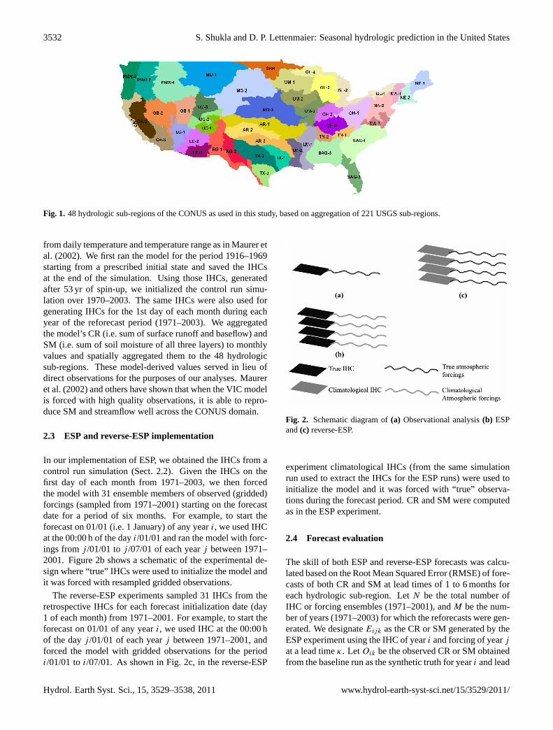
longitude. We then spatially aggregated the forecasts gener-ated by each experiment to the scale of 48 hydrologic sub-regions across the CONUS (Table 1 and Fig. 1). These 48sub-regions were created by merging the 221 US GeologicalSurvey (USGS) hydrologic sub-regions. Each sub-region isnamed after the water resources region in which it is located(Table 1). We compared the spatially aggregated forecastedcumulative runoff (CR) and mean monthly SM with the cor-responding observations (Sect. 2.2) for each sub-region andlead time over the reforecast period. We then estimated aforecast evaluation score (Sect. 2.4) and quantified the con-tributions of the IHCs and FS to seasonal hydrologic forecastskill.

2.1 Model implementation

The VIC model parameterizes the major surface, sub-surface, and land-atmosphere hydrometeorological processesand represents the role of sub-grid spatial heterogeneity inSM, topography, and vegetation on runoff generation (Lianget al., 1994). We ran the model in water balance mode, inwhich the moisture budget is balanced at a daily time step andmodel’s surface temperature is assumed to equal surface airtemperature for purposes of energy flux computations (e.g.,those associated with evapotranspiration and snowmelt). Themodel was run at a daily time step, except for the snow accu-mulation and ablation algorithm, which was run at a 3 h timestep. The1/2 degree parameters (i.e. vegetation, soils, ele-vation and snow band parameters) used in this study are thesame as in Andreadis et al. (2005), which were aggregatedfrom the North America Land Data Assimilation System pa-rameters used in Maurer et al. (2002). The three VIC soillayers had typical depths of∼0.10 m for the first layer, 0.2to 2.3 m for the second layer, and 0.1 to 2.5 m for the thirdlayer. Additional details of the model setup are included inMaurer et al. (2002) and Andreadis et al. (2005).

2.2 Synthetic truth data set

For purposes of evaluating forecast skill, we used a set ofbaseline values of SM and CR, created by a VIC controlrun with gridded observed forcings, as synthetic truth. Weconstructed the standard set of VIC forcings (daily precipita-tion, maximum and minimum temperatures, and wind speed)using methods outlined in Maurer et al. (2002). Precipita-tion and temperature forcings were generated using the In-dex Station method (Wood and Lettenmaier, 2006; Tang etal., 2009) which uses a high quality set of about 2100 pre-cipitation and temperature stations across the CONUS thathave relatively little missing data over our period of analysis.As in Maurer et al. (2002), we used surface wind from thelowest level of the National Centers for Environmental Pro-tection/National Center for Atmospheric Research reanalysis(Kalnay et al., 1996). Other model forcing variables (down-ward solar and longwave radiations, humidity) were derived

www.hydrol-earth-syst-sci.net/15/3529/2011/ Hydrol. Earth Syst. Sci., 15, 3529–3538, 2011


Fig. 1. 48 hydrologic sub-regions of the CONUS as used in this study, based on aggregation of 221 USGS sub-regions.

from daily temperature and temperature range as in Maurer etal. (2002). We first ran the model for the period 1916–1969starting from a prescribed initial state and saved the IHCsat the end of the simulation. Using those IHCs, generatedafter 53 yr of spin-up, we initialized the control run simu-lation over 1970–2003. The same IHCs were also used forgenerating IHCs for the 1st day of each month during eachyear of the reforecast period (1971–2003). We aggregatedthe model’s CR (i.e. sum of surface runoff and baseflow) andSM (i.e. sum of soil moisture of all three layers) to monthlyvalues and spatially aggregated them to the 48 hydrologicsub-regions. These model-derived values served in lieu ofdirect observations for the purposes of our analyses. Maureret al. (2002) and others have shown that when the VIC modelis forced with high quality observations, it is able to repro-duce SM and streamflow well across the CONUS domain.

2.3 ESP and reverse-ESP implementation

In our implementation of ESP, we obtained the IHCs from acontrol run simulation (Sect. 2.2). Given the IHCs on thefirst day of each month from 1971–2003, we then forcedthe model with 31 ensemble members of observed (gridded)forcings (sampled from 1971–2001) starting on the forecastdate for a period of six months. For example, to start theforecast on 01/01 (i.e. 1 January) of any yeari, we used IHCat the 00:00 h of the dayi/01/01 and ran the model with forc-ings fromj /01/01 toj /07/01 of each yearj between 1971–2001. Figure 2b shows a schematic of the experimental de-sign where “true” IHCs were used to initialize the model andit was forced with resampled gridded observations.

The reverse-ESP experiments sampled 31 IHCs from theretrospective IHCs for each forecast initialization date (day1 of each month) from 1971–2001. For example, to start theforecast on 01/01 of any yeari, we used IHC at the 00:00 hof the dayj /01/01 of each yearj between 1971–2001, andforced the model with gridded observations for the periodi/01/01 toi/07/01. As shown in Fig. 2c, in the reverse-ESP

Fig. 2. Schematic diagram of(a) Observational analysis(b) ESPand(c) reverse-ESP.

experiment climatological IHCs (from the same simulationrun used to extract the IHCs for the ESP runs) were used toinitialize the model and it was forced with “true” observa-tions during the forecast period. CR and SM were computedas in the ESP experiment.

2.4 Forecast evaluation

The skill of both ESP and reverse-ESP forecasts was calcu-lated based on the Root Mean Squared Error (RMSE) of fore-casts of both CR and SM at lead times of 1 to 6 months foreach hydrologic sub-region. LetN be the total number ofIHC or forcing ensembles (1971–2001), andM be the num-ber of years (1971–2003) for which the reforecasts were gen-erated. We designateEijk as the CR or SM generated by theESP experiment using the IHC of yeari and forcing of yearjat a lead timeκ. LetOik be the observed CR or SM obtainedfrom the baseline run as the synthetic truth for yeari and lead



Fig. 3. Variation of RMSE ratio (RMSEESP/RMSErevESP) with lead time over 48 hydrologic sub-regions, for the CR forecasts at lead1–6 months, initialized on the beginning of the each month. (DJF: blue, MAM: green, JJA: light brown and SON: red).

timeκ. RMSEESP is then:

RMSEESP=

√√√√ 1

M

[M∑i=1

1

N

N∑j=1

(Oik −Eijk

)2

](1)

Likewise letRijk be the CR or SM generated by the reverse-ESP experiment using the IHC of yearj and forcing of yeari at a lead timeκ so RMSErevESPcan be estimated by:

RMSErevESP=

√√√√ 1

M

[M∑i=1

1

N

N∑j=1

(Oik −Rijk

)2

](2)

We then calculated, the ratio of RMSE of each experiment(Eq. 3).

RMSE Ratio= RMSEESP/RMSErevESP (3)

Unless otherwise specified, we consider that if the ratio isless than 1 then IHCs dominate (in a relative sense) the sea-sonal hydrologic forecast skill and if it is greater than onethen FS dominates.

2.5 κ parameter

Mahanama et al. (2011) introduced a parameter,κ, which isa ratio of the standard deviation of the initial SM+SWE (σw)to the precipitation during the forecast period (σP) (Eq. 4).High κ values correspond to high total moisture variabilityat the time of forecast initialization relative to precipitationvariability during the forecast period and vice versa.κ isbasically a measure of the hydrologic predictability derivedsolely from knowledge of the IHCs at the start of the forecastperiod.

κ = σw/σP (4)

3 Results

In this section we examine the variation of relative contribu-tions of the IHCs and FS in the CR and SM forecast with eachforecast initialization date (i.e. day 1 of each month) for leadtimes of 1 to 6 months across the CONUS. We also highlightthe sub-regions and forecast periods for which improvementin knowledge of IHCs or FS would most improve seasonalhydrologic forecast skill.

3.1 Cumulative runoff forecasts

The variation of RMSE ratio for the forecast of CR at lead1 to 6 months for each of the 48 hydrologic sub-regions isshown in Fig. 3; where CR at lead-1 [lead-6] is the CR overthe first month [1 to 6 months] of the forecast period. RMSEratios below 1.0 indicate that the relative forecast error dueto uncertainties in the FS is lower than the error due to un-certainties in the IHCs; which indicates the relatively highcontribution of the IHCs in the CR forecasts skill.

The variation of the RMSE ratio is much different acrosssub-regions and forecast periods (Fig. 3). The IHCs stronglydominate CR forecasts during winter and spring (Marchand April mainly) months over GL, SRR, UM, and MO-1 sub-regions. The dominance of the IHCs in CR pre-diction over MO-1 sub-region, almost throughout the yearis an observation made by Maurer and Lettenmaier (2003)as well. In the Western US, sub-regions such as PNW,GB, LC, UC, CA, and RG-1, high skill due to the IHCsin lead 1–6 months CR forecasts is mainly apparent duringspring (MAM) and summer (mainly June) months. Woodand Lettenmaier (2008) also found dominance of the IHCsin the seasonal runoff forecast during winter/spring tran-sition months over two Western US basins. This finding



Fig. 4. Plot of the maximum lead (in months) at which RMSE Ratiois less than 1, for CR forecasts, initialized on the beginning of eachmonth.

suggests that runoff forecasts in the above-mentioned sub-regions and forecast periods could benefit substantially fromimprovements in knowledge of the IHCs. For sub-regionsin the Eastern US such as NE, MA, SAG-1 and -2, OH-1 and -2, and UM, RMSE ratios are less than one forlead 1–2 months, for CR forecasts initialized during win-ter – (December-January-February (DJF) – and spring month(March and April, mainly). This finding is in agreement withLi et al. (2009) who noted that the IHCs dominate the stream-flow (and SM) forecasts made during January and July, overOhio and Southeastern US sub-regions, up to lead 1 month.These sub-regions as well could potentially benefit from im-provements in estimates of the IHCs during these seasons.Aside from those months and locations, FS dominates theCR forecasts. Some sub-regions such as TN, LM, and SAG-3 stand out because their RMSE ratios throughout the entireyear and for all lead times exceeds 1, which suggests thatin those sub-regions improved hydrologic forecasts must, forthe most part, await improvements in FS.

There is also a clear difference between the variations ofRMSE ratio initialized from wet vs dry IHCs. For example,in most sub-regions across the CONUS, forecasts initializedduring summer months have RMSE ratios less than or equalto 1 for lead-1 month CR forecasts (also shown by Wood andLettenmaier, 2008 and Li et al., 2009) for forecasts initial-ized during summer months. Furthermore the rate of changein the RMSE ratio for 1-month vs. 6-month forecasts is muchhigher in forecasts initialized in the summer months than inwinter and spring months when the IHCs are generally wet.This property is particularly significant for predictions dur-ing droughts when the IHCs are dry. It potentially meansthat during a drought event when the IHCs are dry, the sig-nal from the IHCs may dominate even at lags for which theRMSE ratio exceeds 1. Additionally, in climatologically wet

periods followed by dry initial conditions, FS may well beimportant in improving seasonal hydrologic forecasts.

Figure 4 shows the maximum lead time (in months) atwhich the RMSE ratio of CR forecasts is below 1; definingthe maximum lead time the IHCs can play a significant rolein CR forecasts relative to FS. Beyond this lead, FS dom-inates the CR forecast skill; hence improvement in the FSwould lead to higher forecast skill. For the most part, thesub-regions in Northeastern and Southeastern US would ben-efit most from improvements in FS throughout the year be-cause the IHCs dominate up to lead-2 only. In the mountain-ous west and Pacific Coast sub-regions FS dominates mainlyduring fall and winter. On the other hand, IHCs dominatein those sub-regions during spring and summer for up to6 months lead time. GL, SRR, and UM sub-regions over-all would benefit most from improvement in knowledge ofIHCs during winter and spring months (mainly March) andFS during summer months.

3.2 Soil moisture forecasts

SM is a key hydrologic state variable, and a natural indicatorof agricultural drought. Figure 5 show the RMSE ratios ofthe mean monthly SM forecast, at lead-1 (i.e. mean monthlySM of the first month) to 6 (i.e. mean monthly SM of the 6thmonth of the forecast period) for forecasts initialized on thebeginning of each month. In contrast to forecasts of CR, theRMSE ratio at lead-1 is almost always less than 1, across theCONUS and for each forecast period, indicating the strongdominance of IHCs for short lead forecasts. The ratio in-creases for leads greater than 1.

In the NE, MA, SAG, OH, LM, and TN sub-regions the in-fluence of IHCs beyond lead-1 is generally negligible, whichin turn means that improvement in FS will be required toimprove SM forecasts beyond lead-1. This pattern for SMforecasts was also shown by Li et al. (2009) in the Ohio andsoutheastern regions. Conversely, in the majority of the sub-regions in the Midwestern US, such as GL-1, -2, -3; SRR,UM, and the Western US show strong IHC influence for SMforecasts up to lead-5, when the forecast is initialized in win-ter or spring months. In snowmelt-dominated sub-regionsin the Western US, the skill of SM forecasts during springand summer months is especially high. In UC, LC, PNW,GB, and CA sub-regions, useful skill in SM forecasts canbe derived from the IHCs for leads as long as 6 months forforecasts initialized during the summer months.

Overall, the relative contributions of IHCs are greater forforecasts of SM than for forecasts of CR at lead-1 month.The contribution of IHCs is dominant over the Western US,in particular during spring and summer months.

Following the same criterion as we used for CR forecasts,Fig. 6 shows the maximum lead time at which the RMSEratio is below 1 for mean monthly SM forecasts. In generalmost of the sub-regions have some SM forecasts skill derivedby the IHCs, at least up to lead-1 (including sub-regions in



Fig. 5. Variation of RMSE ratio (i.e. RMSEESP/RMSErevESP) with lead time over 48 hydrologic sub-regions, for the SM forecasts at lead-1to 6 months, initialized on the beginning of the each month. (DJF: blue, MAM: green, JJA: light brown and SON: red).

Fig. 6. Plot of the maximum lead (in months) at which RMSE Ratiois less than 1, for mean monthly SM forecasts, initialized on thebeginning of each month.

Northeastern and Southeastern US). This means that the rela-tive contribution of the IHCs in the SM forecasts is more ex-tensive than in the CR forecasts during the first month of theforecast period (i.e. lead-1). The spatial contrast between thesub-regions and forecast periods with high and low values ofmaximum lead time, where IHCs significantly influence theSM forecasts skill, is similar to CR forecasts.

3.3 Controls on hydrologic forecast skill

Mahanama et al. (2011) found a first order relationship be-tween IHC-based 3-month streamflow forecasts (that is, fore-casts wherein CR was regressed on the IHCs) andκ. Fol-lowing their analogy we expect a first order relationship be-

tween the inverse RMSE ratio (i.e. RMSErevESP/RMSEESP)andκ. Namely, we expect that RMSEESPshould be smallerfor sub-regions and forecast periods with higherκ. Scatter ofthe inverse RMSE ratio andκ are shown for forecast periodsof 1, 3, and 6 months in Fig. 7a–c, respectively. Red cir-cles and blue circles show the inverse RMSE ratio estimatedacross all the hydrologic sub-regions and forecast initializa-tion dates for the forecast of CR and mean monthly SM atlead-1, lead-3, and lead-6 (Fig. 7a–c, respectively). The val-ues ofκ vary for different forecast periods, and in general,the number of hydrologic sub-regions and forecast periodswith k > 1 decreases as the lead time increases. First orderrelationships between the inverse RMSE ratio andκ clearlyexist at each lead time. The range of inverse RMSE ratios fora givenκ value seems to be higher for CR at lead-1 than forSM (Fig. 7a). Overall at lead-1, the inverse RMSE ratio ishigher for SM than for CR. The values of the inverse RMSEratio of SM and CR forecast is much more comparable inlead-3 forecast (Fig. 7b). The inverse RMSE ratio for lead-6,CR forecast is generally higher than its corresponding valuesfor SM forecasts at lead-6 (Fig. 7c).

4 Summary and conclusions

The two key factors influencing seasonal CR and SM forecastskill are IHCs and FS. In order to improve seasonal hydro-logic forecast skill in the CONUS, it is important to under-stand the seasonal and spatial variability of relative contribu-tions of these components. We performed two modeling ex-periments – ESP and reverse-ESP – in which the hydrologicprediction skill exploits knowledge of IHCs and FS respec-tively to quantify the relative contributions of each factorsand to identify the sub-regions and forecast periods which



Fig. 7. Inverse RMSE ratio (i.e. RMSErevESP/RMSEESP) of CRand mean monthly SM forecasts at(a) lead-1(b) lead-3, and(c)lead-6 plotted againstκ parameter of each forecast period (i.e. 1month, 3 months, and 6 months, respectively).

can benefit most from improvements in the FS or knowledgeof the IHCs. Our key findings are:

1. IHCs generally have the strongest influence over CRand SM forecasts at lead-1, beyond which their influ-ence decays at rates that depend on location, lead time,and forecast initialization date.

2. Beyond lead-1, IHCs primarily influence the CR andSM forecasts during spring and summer months, mostlyover the Western US.

3. FS dominates CR and SM forecast skill beyond lead-1 mainly over the Northeastern and Southeastern USthroughout the year. For the rest of the CONUS, FSgenerally dominates CR and SM forecasts during falland early winter months.

4. The relative contributions of IHCs and FS have a firstorder relationship with the ratio of initial total moisturevariability to the variability of precipitation during theforecast period for the temporal scale of seasonal hy-drologic prediction.

While the ESP-based framework used in this study allowsa consistent estimation of the contribution of the IHCs andFS over large spatial scale (e.g. continental scale) and longtime period, it is important to understand the limitations of

the study design. The distribution of FS (in the ESP exper-iment) and IHCs (in the reverse-ESP experiment) is uncon-ditional (i.e. climatological distribution) and we assume thatIHCs (in the ESP experiment) and FS (in the reverse-ESP ex-periment) are perfect, hence our results arguably provide anupper bound on the contributions of the IHCs and FS to sea-sonal hydrologic prediction skill. Furthermore since we donot route the runoff through the stream network and ratheruse spatially aggregated values, there will be some differ-ence in the spatial extent and lead time of the contributionof IHCs (mainly snow-melt) in streamflow based on the timeof concentration of a given basin, although this effect can beexpected to be limited, for the most part, to about a month.

We believe the findings of this study could have impor-tant implications for the improvement of seasonal hydro-logic and drought prediction in the CONUS. We identifiedthe sub-regions and forecast periods during which improve-ment in the knowledge of IHCs and FS could result in themost improvement in seasonal hydrologic prediction skill.For those river basins and forecast periods which have a sub-stantial contribution of IHCs to seasonal hydrologic predic-tion skill, for instance, skill improvements might be derivedby improving the IHCs – for example through the assimila-tion of ground based or remote sensing data. Another pos-sible way of improving seasonal hydrologic forecasts withrelatively short leads may be to exploit the skill of mediumrange weather forecasts over the first 1–2 weeks of the fore-cast period.

Appendix A

Abbreviations used

AR Arkansas-White-RedCA CaliforniaFS Climate Forecast SkillCONUS Conterminous United StatesCR Cumulative RunoffDJF December-January-FebruaryESP Ensemble Streamflow PredictionGB Great BasinGL Great LakesIHC Initial Hydrologic ConditionsJJA June-July-AugustLC Lower ColoradoLM Lower MississippiLSM Land Surface ModelMA Mid-AtlanticMAM March-April-MayMO MissouriNE New EnglandOH OhioPNW Pacific Northwest



RG Rio GrandeRMSE Root Mean Square ErrorSAG South Atlantic-GulfSM Soil MoistureSON September-October-NovemberSRR Souris-Red-RainySWE Snow Water EquivalentSWM Surface Water MonitorTN TennesseeTX Texas-GulfUC Upper ColoradoUM Upper MississippiUSGS United States Geological SurveyVIC Variable Infiltration Capacity

Acknowledgements.We thank Elizabeth Clark, Ben Livneh andMohammad Safeeq for their valuable comments and suggestionson earlier versions of this paper. This research was supported inpart by the National Oceanic and Atmospheric Administration(NOAA) grants No. NA08OAR4320899 and NA08OAR4310210to the University of Washington.

Edited by: J. Seibert

References

Adam, J. C., Haddeland, I., Su, F. and Lettenmaier, D. P.: Simu-lation of reservoir influences on annual and seasonal streamflowchanges for the Lena, Yenisei, and Ob’rivers, J. Geophys. Res.,112, D24114, 2007.

Andreadis, K. and Lettenmaier, D.: Assimilating remotely sensedsnow observations into a macroscale hydrology model, Adv. Wa-ter Resour., 29, 872–886, 2006.

Andreadis, K. M., Clark, E. A., Wood, A. W., Hamlet, A. F. andLettenmaier, D. P.: 20th century drought in the conterminousUnited States, J. Hydrometeorol., 6, 985–1001, 2005.

Cherkauer, K. A., Bowling, L. C., and Lettenmaier, D. P.: Vari-able infiltration capacity cold land process model updates, GlobalPlanet Change, 38, 151–159, 2003.

Clark, M. P., Slater, A. G., Barrett, A. P., Hay, L. E., McCabe, G.J., Rajagopalan, B., and Leavesley, G. H.: Assimilation of snowcovered area information into hydrologic and landsurface mod-els, Adv. Water Resour., 29, 1209–1221, 2006.

Hayes, M., Svoboda, M., Le Comte, D., Redmond, K., and Pas-teris, P.: Drought monitoring:New tools for the 21st century, in:Drought and Water Crises: Science, Technology, and Manage-ment Issues, edited by: Wihite, D. A., Taylor and Francis, BocaRaton (LA), 53–69, 2005.

Kalnay, E. C., Kanamitsu, M., Kistler, R., Collins, W., Deaven, D.,Gandin, L., Iredell, M., Saha,S., White, G., Woollen, J., Zhu, Y.,Chelliah, M., Ebisuzaki, W., Higgins, W., Janowiak, J., Mo,K.C., Ropelewski, C., Wang, J., Leetmaa, A., Reynolds, R., Jenne,R., and Joseph, D.: The NCEP/NCAR 40 yr reanalysis project,B. Am. Meteorol. Soc., 77, 437–472, 1996.

Koster, R. D., Mahanama, S. P. P., Livneh, B., Lettenmaier, D. P.,and Reichle, R. H.: Skill in streamflow forecasts derived fromlarge-scale estimates of soil moisture and snow, Nat. Geosci., 3,613–616, 2010.

Krishnamurti, T. N., Kishtawal, C. M., LaRow, T. E., Bachiochi, D.R., Zhang, Z., Williford, C. E., Gadgil, S., and Surendran, S.: Im-proved weather and seasonal climate forecasts from multimodelsuperensemble, Science, 285, 1548–1550, 1999.

Li, H., Luo, L., and Wood, E. F.: Seasonal hydrologic predictions oflow-flow conditions over Eastern USA during the 2007 drought,Atmos. Sci. Lett., 9, 61–66, 2008.

Li, H., Luo, L., Wood, E. F., and Schaake, J.: Therole of initial conditions and forcing uncertainties in sea-sonal hydrologic forecasting, J. Geophys. Res., 114, D04114,doi:10.1029/2008JD010969, 2009.

Liang, X., Lettenmaier, D. P., Wood, E. F., and Burges, S. J.: Asimple hydrologically based model of land surface water and en-ergy fluxes for general circulation models, J. Geophys. Res., 99,14415–14428, 1994.

Luo, L. and Wood, E. F.: Monitoring and predictingthe 2007 US drought, Geophys. Res. Lett., 34, L22702,doi:10.1029/2007GL031673, 2007.

Mahanama, S. P., Livneh, B., Koster, R. D., Lettenmaier, D. P., andReichle, R. H.: Soil Moisture, Snow, and Seasonal StreamflowForecasts in the United States, e-View,doi:10.1175/JHM-D-11-046.1, 2011

Maurer, E. P. and Lettenmaier, D. P.: Predictability of seasonalrunoff in the Mississippi River basin, J. Geophys. Res., 108,8607,doi:10.1029/2002JD002555, 2003.

Maurer, E. P., Wood, A. W., Adam, J. C., Lettenmaier, D. P., andNijssen, B.: A Long-Term Hydrologically Based Dataset of LandSurface Fluxes and States for the Conterminous United States, J.Climate, 15, 3237–3251, 2002.

Maurer, E. P., Lettenmaier, D. P., and Mantua, N. J.: Variabilityand potential sources of predictability of North American runoff,Water Resour. Res., 40, W09306,doi:10.1029/2003WR002789,2004.

Maurer, E. P., O’Donnell, G. M., Lettenmaier, D. P. andRoads, J. O.: Evaluation of the land surface water bud-get in NCEP/NCAR and NCEP/DOE reanalyses using an off-line hydrologie model, J. Geophys. Res., 106, 17841–17862,doi:10.1029/2000JD900828, 2001.

McGuire, M., Wood, A. W., Hamlet, A. F., and Lettenmaier, D. P.:Use of satellite data for streamflow and reservoir storage fore-casts in the Snake River Basin, J. Water Res. Pl.-ASCE, 132, 97,2006.

Nijssen, B., O’Donnell, G. M., Hamlet, A. F. and Lettenmaier, D.P.: Hydrologic sensitivity of global rivers to climate change, Cli-matic Change, 50, 143–175, 2001.

Stefanova, L. and Krishnamurti, T. N.: Interpretation of SeasonalClimate Forecast Using Brier Skill Score, The Florida State Uni-versity Superensemble, and the AMIP-I Dataset, J. Climate, 15,537–544, 2002.

Svoboda, M., LeComte, D., Hayes, M., Heim, R., Gleason, K.,Angel, J., Rippey, B., Tinker, R., Palecki, M., Stooksbury, D.,Miskus, D., and Stephens, S.: The Drought Monitor, B. Am.Meteor. Soc., 83, 1181–1190, 2002.

Tang, Q., Wood, A. W., and Lettenmaier, D. P.: Real-Time Precipi-tation Estimation Based on Index Station Percentiles, J. Hydrom-eteorol., 10, 266–277,doi:10.1175/2008JHM1017.1, 2009.

Wang, A., Bohn, T. J., Mahanama, S. P., Koster, R. D. and Letten-maier, D. P.: Multimodel Ensemble Reconstruction of Droughtover the Continental United States, J. Climate, 22, 2694–2712,


http://dx.doi.org/10.1029/2008JD010969

http://dx.doi.org/10.1029/2007GL031673

http://dx.doi.org/10.1175/JHM-D-11-046.1

http://dx.doi.org/10.1175/JHM-D-11-046.1

http://dx.doi.org/10.1029/2002JD002555

http://dx.doi.org/10.1029/2003WR002789

http://dx.doi.org/10.1029/2000JD900828

http://dx.doi.org/10.1175/2008JHM1017.1


doi:10.1175/2008JCLI2586.1, 2009.Wood, A. W.: The University of Washington Surface Water Mon-

itor: An experimental platform for national hydrologic assess-ment and prediction, in Proceedings AMS 22nd Conference onHydrology, New Orleans, LA, 20–24 January 2008, 2008.

Wood, A. W. and Lettenmaier, D. P.: A test bed for new seasonalhydrologic forecasting approaches in the Western United States,B. Am. Meteorol. Soc., 87, 1699–1712, 2006.

Wood, A. W. and Lettenmaier, D. P.: An ensemble approach forattribution of hydrologic prediction uncertainty, Geophys. Res.Lett., 35, L14401,doi:10.1029/2008GL034648, 2008.

Wood, A. W., Maurer, E. P., Kumar, A., and Lettenmaier,D. P.: Long-range experimental hydrologic forecasting forthe Eastern United States, J. Geophys. Res., 107, 4429,doi:10.1029/2001JD000659, 2002.


http://dx.doi.org/10.1175/2008JCLI2586.1

http://dx.doi.org/10.1029/2008GL034648

http://dx.doi.org/10.1029/2001JD000659

seasonal hydrologic prediction in the united states

Documents