1075

Journal of Oceanography, Vol. 61, pp. 1075 to 1087, 2005

Keywords:⋅⋅⋅⋅⋅ Ocean carboncycle,

⋅⋅⋅⋅⋅ Oyashio region,⋅⋅⋅⋅⋅ climatology,⋅⋅⋅⋅⋅ chemical tracer.

* Corresponding author. E-mail: tono@fra.affrc.go.jp

† Present address: 1-15-422 Minai-7, Nishi-23, Chuo-ku, Sapporo 064-

0807, Japan.

Copyright © The Oceanographic Society of Japan.

Seasonal and Interannual Variation of DIC in SurfaceMixed Layer in the Oyashio Region: A ClimatologicalView

TSUNEO ONO1*, HIROMI KASAI1, TAKASHI MIDORIKAWA2, YUSUKE TAKATANI3, KAZUHIRO SAITO4,MASAO ISHII2, YUTAKA W. WATANABE5 and KATSUYUKI SASAKI6†

1Hokkaido National Fisheries Research Institute, Katsurakoi, Kushiro 085-0802, Japan2Meteorological Research Institute, Nagamine, Tsukuba 305-0052, Japan3Hakodate Marine Observatory, Mihara, Hakodate 041-0806, Japan4Kobe Marine Observatory, Wakihama-kaigandori, Chuo-ku, Kobe 651-0073, Japan5Graduate School of Environmental Earth Science, Hokkaido University, Chuo-ku, Sapporo 060-0810, Japan6National Research Institute of Fisheries Science, Fukuura, Kanazawa-ku, Yokohama 236-8648, Japan

(Received 19 November 2004; in revised form 15 April 2005; accepted 15 April 2005)

Eight-year observation results of DIC from 1996 to 2003 in the Oyashio region havebeen analyzed to obtain a climatological view of its seasonal variation and interannualvariation. Data of DIC obtained by several institutes are synthesized to give a datasetwith an uncertainty lower than 5 µµµµµmol/kg. The obtained climatology of NDIC sea-sonal variation in the Oyashio mixed layer shows a seasonal amplitude of 176µµµµµmol/kg, with a maximum in January and a minimum in September. These featuresclosely resemble those observed in the southern half of the western subarctic NorthPacific (WSNP) including Station KNOT, although the timing of the NDIC maximumis slightly advanced in the case of the Oyashio. Analysis using a quasi-conservativetracer Cp0 (NDIC - 106NP) shows that among 176 µµµµµmol/kg of NDIC seasonal varia-tion, only 16 µµµµµmol/kg is attributed to hydrographic processes while the remaining160 µµµµµmol/kg is attributed to biological processes. The Cp0 value in the Oyashio mixedlayer also resembles that of the WSNP mixed layer during the months May to Novem-ber, suggesting further resemblance of the Oyashio water mass to that of WSNP interms of carbon dynamics. The present results also suggest that a single data ob-tained in Oyashio mixed layer contains 30 µµµµµmol/kg of potential uncertainty for therepresentativity of this region, which leads to a note about a need to treat with cau-tion results obtained by a single observation in this region.

Long-period variation has also been stated to occur in itssubsurface in relation to the long-term water circulationchange (e.g., Andreev and Kusakabe, 2001; Ono et al.,2001; Watanabe et al., 2001; Andreev and Watanabe,2002; Emerson et al., 2004). A distinct amount of anthro-pogenic carbon is pumped down from the mixed layer ofthis region into the North Pacific Intermediate Water(Tsunogai et al., 1993; Ono et al., 2000a, 2003; Andreevet al., 2001), the formation rate of which, and hence theannual flux of anthropogenic carbon, is also expected tobe changed by long-term water circulation change(Watanabe et al., 2001; Ono et al., 2002, 2003). TheOyashio region, the westernmost branch of the WSNP, isa good candidate for the assessment of such carbon dy-

1. IntroductionThe Western Subarctic North Pacific (WSNP) is an

important oceanic zone in the oceanic natural and/or an-thropogenic carbon cycle. Dissolved inorganic carbon(DIC) in the mixed layer shows a large seasonal varia-tion of up to 140~160 µmol/kg (Tsurushima et al., 2002;Wong et al., 2002) due to strong vertical mixing in win-ter and subsequent great biological activity in spring.

1076 T. Ono et al.

namics, since carbon parameters and related chemicalspecies, such as nutrients, have been measured along sev-eral repeat observation lines. Although we have a two-year time series data from station KNOT in the center ofWSNP (Nojiri, 1998; Tsurushima et al., 2002; Imai et al.,2002), the Oyashio region has over 30 years of time se-ries data for several hydrographic/geochemical parameters

(e.g., Ono et al., 2001, 2002; Chiba et al., 2004; Tadokoroet al., 2005). Furthermore, several institutes have mea-sured DIC in this region from 1996 to the present, theaggregate of which gives an eight-year time series. Themain purpose of this paper is therefore 1) to compile cur-rent DIC data in this region to obtain a climatologicalview of its seasonal variation; and 2) to assess both simi-

*See the text for each acronym of PIs.

Cruise ID Cruise date No. of Stns. forOyashio DIC

PI/water sampling PI/measurement Area

<cross-section observation>HK9605 1996.05.08–05.17 4 HNFRI HU AlineSY9701 1997.01.13–02.14 3 NRIFS NRIFS Near-AlineSY9705 1997.05.09–05.18 2 NRIFS NRIFS Near-AlineTK9804 1998.04.13–04.30 6 HNFRI NRIFS AlineHK0101 2001.01.13–01.18 2 HNFRI MRI AlineTK0104 2001.04.17–04.24 1 HNFRI MRI AlineKO01-04 2001.04.20–05.15 1 HMO MRI Near-AlineHK0105 2001.05.08–05.14 2 HNFRI MRI AlineKO01-06 2001.06.12–07.25 3 HMO MRI Near-AlineTK0110 2001.10.05–10.10 1 HNFRI MRI AlineKO01-11 2001.11.16–12.10 2 HMO MRI Near-AlineTK0201 2002.01.18–01.22 2 HNFRI MRI AlineKO02-01 2002.01.25–03.05 1 HMO MRI Near-AlineTK0203 2002.03.13–03.18 1 HNFRI MRI AlineTK0204 2002.04.16–04.25 1 HNFRI MRI AlineKO02-04 2002.04.26–05.18 3 HMO MRI Near-AlineHK0205 2002.05.10–05.23 5 HNFRI HU AlineTK0207 2002.07.05–07.14 2 HNFRI HU AlineHK0210 2002.10.01–10.10 2 HNFRI HU AlineHK0301 2003.01.15–01.22 2 HNFRI HNFRI AlineTK0303 2003.03.14–03.20 2 HNFRI HNFRI AlineTK0304 2003.04.15–04.27 2 HNFRI HNFRI AlineHK0305 2003.05.09–05.23 2 HNFRI HNFRI Aline

<surface observation>KO98-04 1998.04.28–05.29 32 HMO MRI Entire OyashioKO98-06 1998.06.10–08.10 23 HMO MRI Entire OyashioKO98-10 1998.10.06–11.05 8 HMO MRI Entire OyashioKO98-11 1998.11.11–12.10 8 HMO MRI Entire OyashioKO00-02 2000.02.01–03.03 8 HMO MRI Entire OyashioKO00-04 2000.04.28–05.17 7 HMO MRI Entire OyashioKO00-06 2000.06.24–08.10 25 HMO MRI Entire OyashioKO00-09 2000.09.29–10.23 12 HMO MRI Entire OyashioKO00-11 2000.11.07–12.07 15 HMO MRI Entire OyashioKO01-02 2001.02.07–02.23 22 HMO MRI Entire OyashioKO01-04 2001.04.20–05.15 28 HMO MRI Entire OyashioKO01-06 2001.06.12–07.25 27 HMO MRI Entire OyashioKO01-09 2001.09.27–10.30 18 HMO MRI Entire OyashioKO01-11 2001.11.16–12.10 20 HMO MRI Entire OyashioKO02-01 2002.01.25–03.05 22 HMO MRI Entire OyashioKO02-04 2002.04.26–05.18 36 HMO MRI Entire Oyashio

Table 1. List of cruises considered in this study.

DIC in the Oyashio Region 1077

37

38

39

40

41

42

43

44

141 142 143 144 145 146 147 148 149

Lat

itude

(oN

)

Longitude (oE)

Hokkaido

Honsh

u

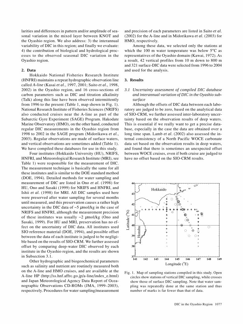
Fig. 1. Map of sampling stations compiled in this study. Opencircles show stations of vertical DIC sampling, while crossesshow those of surface DIC sampling. Note that water sam-pling was repeatedly done at the same station and thusnumber of marks is far fewer than that of data.

larities and differences in pattern and/or amplitude of sea-sonal variation in the mixed layer between KNOT andthe Oyashio region. We also address: 3) the interannualvariability of DIC in this region; and finally we evaluate:4) the contribution of biological and hydrological proc-esses to the observed seasonal DIC variation in theOyashio region.

2. DataHokkaido National Fisheries Research Institute

(HNFRI) maintains a repeat hydrographic observation linecalled A-line (Kasai et al., 1997, 2001; Saito et al., 1998,2002) in the Oyashio region, and 16 cross-sections ofcarbon parameters such as DIC and titration alkalinity(Talk) along this line have been observed intermittentlyfrom 1996 to the present (Table 1, map shown in Fig. 1).National Research Institute of Fisheries Sciences (NRIFS)also conducted cruises near the A-line as part of theSubarctic Gyre Experiment (SAGE) Program. HakodateMarine Observatory (HMO), on the other hand, conductedregular DIC measurements in the Oyashio region from1998 to 2002 in the SAGE program (Midorikawa et al.,2003). Regular observations are made of surface waters,and vertical observations are sometimes added (Table 1).We have compiled these databases for use in this study.

Four institutes (Hokkaido University (HU), NRIFS,HNFRI, and Meteorological Research Institute (MRI), seeTable 1) were responsible for the measurement of DIC.The measurement technique is basically the same for allthese institutes and is similar to the DOE standard method(DOE, 1994). Detailed methods for water sampling andmeasurement of DIC are listed in Ono et al. (1998) forHU, Ono and Sasaki (1999) for NRIFS and HNFRI, andIshii et al. (1998) for MRI. All DIC samples used herewere preserved after water sampling for several monthsuntil measured, and this preservation causes a rather highuncertainty in the DIC data of ~5 µmol/kg in the case ofNRIFS and HNFRI, although the measurement precisionof these institutes was usually ~2 µmol/kg (Ono andSasaki, 1999). For HU and MRI, preservation has no ef-fect on the uncertainty of DIC data. All institutes usedSIO reference material (DOE, 1994), and possible offsetbetween the data of each institute is judged to be negligi-ble based on the results of SIO-CRM. We further assessedoffset by comparing deep-water DIC observed by eachinstitute in the Oyashio region, and the results are shownin Subsection 3.1.

Other hydrographic and biogeochemical parameterssuch as salinity and nutrient are routinely measured bothon the A-line and HMO cruises, and are available at theA-line HP (http://ss.hnf.affrc.go.jp/a-line/index_e.html)and Japan Meteorological Agency Data Report of Ocea-nographic Observations CD-ROMs (JMA, 1999–2003),respectively. Procedures for water sampling/measurement

and precision of each parameters are listed in Saito et al.(2002) for the A-line and in Midorikawa et al. (2003) forHMO, respectively.

Among these data, we selected only the stations atwhich the 100 m water temperature was below 5°C asrepresentatives of the Oyashio domain (Kawai, 1972). Asa result, 42 vertical profiles from 10 m down to 800 mand 321 surface-DIC data were selected from 1996 to 2004and used for the analysis.

3. Results

3.1 Uncertainty assessment of compiled DIC databaseand interannual variation of DIC in the Oyashio sub-surfaceAlthough the offsets of DIC data between each labo-

ratory are judged to be zero, based on the analytical dataof SIO-CRM, we further assessed inter-laboratory uncer-tainty based on the observation results of deep waters.This is essential if we really want to get a precise data-base, especially in the case the data are obtained over along time span. Lamb et al. (2002) also assessed the in-ternal consistency of a North Pacific WOCE carbonatedata set based on the observation results in deep waters,and found that there is sometimes an unexpected offsetbetween WOCE cruises, even if both cruise are judged tohave no offset based on the SIO-CRM results.

1078 T. Ono et al.

Data of five sections observed along the A-line inMay (HK9605, SY9705, HK0105, HK0205, andHK0305), in which DIC are measured by four differentlaboratories (Table 1), were selected and plotted in thesingle T-S diagram shown as Fig. 2(a). The area wheredata of all five cruises overlap are cut from the whole(Fig. 2(b)) and the data in this selected area are re-plot-ted into a density-T field (Fig. 2(c)). Finally, data on asingle density-T profile are chosen from the density-Tfield as a “virtual standard water column (VSWC)” (Fig.2(d)). In this final data selection, shape of the VSWC plotis determined ad hoc so that as many data as possiblefrom each cruise are retained in the VSWC. DIC datacorresponding to the T-S data on VSWC are then plottedagainst density (Fig. 3(a)) or corresponding silicate data(Fig. 3(b)) to check the offset.

In the VSWC dataset, DIC on isopycnals below27.2σθ (ca. below ~600 m depth) show a standard devia-tion of ~5 µmol/kg, or the same value as that of the meas-urement uncertainty of NRIFS/HNFRI data. DIC valuesin a silicate concentration horizon larger than 100µmol/kg also show a constant standard deviation of ~5µmol/kg. From these results, we conclude that the offsetof DIC among four institutes is less than 5 µmol/kg, orbelow the measurement uncertainty during these eightyears.

Figure 3(a) also shows that the standard deviation ofDIC does not increase from 5 µmol/kg even in the 26.65σθisopycnals, suggesting that the interannual variation ofDIC was lower than this value during these years. Theanthropogenic increase of DIC corresponding to the in-crease of atmospheric carbon dioxide concentration is

Fig. 2. Schematic diagram to compose a “virtual standard water column (VSWC)” profile from the observed data. a) All the dataare plotted on a T-S diagram. b) Data in the area where data of all five cruises overlap are cut from the whole T-S field, and c)then the data selected in b) are re-plotted on a density-temperature diagram. d) Finally, a single density-temperature profile isselected as VSWC so that as many data of five cruises as possible remained in VSWC (by eye). Symbols represent dataobserved in 1996 (solid circles), 1997 (open circles), 2001 (Xs), 2002 (crosses), and 2003 (open triangles), respectively.

DIC in the Oyashio Region 1079

2000 2100 2200 2300 240026.0

26.4

26.8

27.2

27.6

a)

DIC(µmol/kg)p

ote

nti

al d

ensi

ty (

σ θ)

2000

2100

2200

2300

2400

0 40 80 120 160

b)

DIC

(µm

ol/

kg

)

Si (µmol/kg)

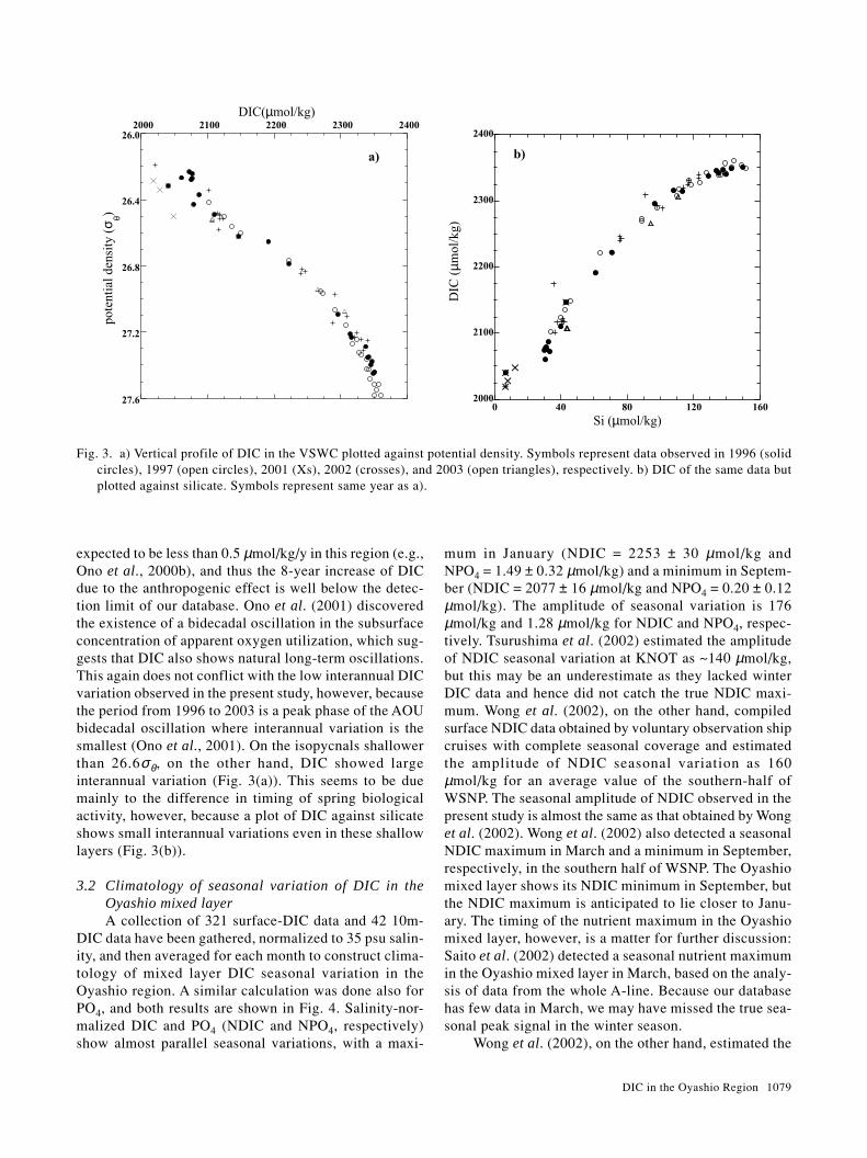
Fig. 3. a) Vertical profile of DIC in the VSWC plotted against potential density. Symbols represent data observed in 1996 (solidcircles), 1997 (open circles), 2001 (Xs), 2002 (crosses), and 2003 (open triangles), respectively. b) DIC of the same data butplotted against silicate. Symbols represent same year as a).

expected to be less than 0.5 µmol/kg/y in this region (e.g.,Ono et al., 2000b), and thus the 8-year increase of DICdue to the anthropogenic effect is well below the detec-tion limit of our database. Ono et al. (2001) discoveredthe existence of a bidecadal oscillation in the subsurfaceconcentration of apparent oxygen utilization, which sug-gests that DIC also shows natural long-term oscillations.This again does not conflict with the low interannual DICvariation observed in the present study, however, becausethe period from 1996 to 2003 is a peak phase of the AOUbidecadal oscillation where interannual variation is thesmallest (Ono et al., 2001). On the isopycnals shallowerthan 26.6σθ, on the other hand, DIC showed largeinterannual variation (Fig. 3(a)). This seems to be duemainly to the difference in timing of spring biologicalactivity, however, because a plot of DIC against silicateshows small interannual variations even in these shallowlayers (Fig. 3(b)).

3.2 Climatology of seasonal variation of DIC in theOyashio mixed layerA collection of 321 surface-DIC data and 42 10m-

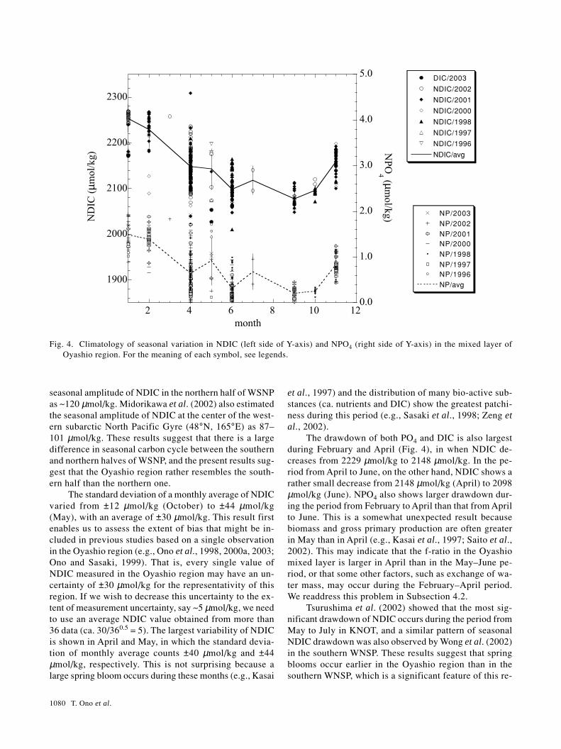
DIC data have been gathered, normalized to 35 psu salin-ity, and then averaged for each month to construct clima-tology of mixed layer DIC seasonal variation in theOyashio region. A similar calculation was done also forPO4, and both results are shown in Fig. 4. Salinity-nor-malized DIC and PO4 (NDIC and NPO4, respectively)show almost parallel seasonal variations, with a maxi-

mum in January (NDIC = 2253 ± 30 µmol/kg andNPO4 = 1.49 ± 0.32 µmol/kg) and a minimum in Septem-ber (NDIC = 2077 ± 16 µmol/kg and NPO4 = 0.20 ± 0.12µmol/kg). The amplitude of seasonal variation is 176µmol/kg and 1.28 µmol/kg for NDIC and NPO4, respec-tively. Tsurushima et al. (2002) estimated the amplitudeof NDIC seasonal variation at KNOT as ~140 µmol/kg,but this may be an underestimate as they lacked winterDIC data and hence did not catch the true NDIC maxi-mum. Wong et al. (2002), on the other hand, compiledsurface NDIC data obtained by voluntary observation shipcruises with complete seasonal coverage and estimatedthe amplitude of NDIC seasonal variation as 160µmol/kg for an average value of the southern-half ofWSNP. The seasonal amplitude of NDIC observed in thepresent study is almost the same as that obtained by Wonget al. (2002). Wong et al. (2002) also detected a seasonalNDIC maximum in March and a minimum in September,respectively, in the southern half of WSNP. The Oyashiomixed layer shows its NDIC minimum in September, butthe NDIC maximum is anticipated to lie closer to Janu-ary. The timing of the nutrient maximum in the Oyashiomixed layer, however, is a matter for further discussion:Saito et al. (2002) detected a seasonal nutrient maximumin the Oyashio mixed layer in March, based on the analy-sis of data from the whole A-line. Because our databasehas few data in March, we may have missed the true sea-sonal peak signal in the winter season.

Wong et al. (2002), on the other hand, estimated the

1080 T. Ono et al.

seasonal amplitude of NDIC in the northern half of WSNPas ~120 µmol/kg. Midorikawa et al. (2002) also estimatedthe seasonal amplitude of NDIC at the center of the west-ern subarctic North Pacific Gyre (48°N, 165°E) as 87–101 µmol/kg. These results suggest that there is a largedifference in seasonal carbon cycle between the southernand northern halves of WSNP, and the present results sug-gest that the Oyashio region rather resembles the south-ern half than the northern one.

The standard deviation of a monthly average of NDICvaried from ±12 µmol/kg (October) to ±44 µmol/kg(May), with an average of ±30 µmol/kg. This result firstenables us to assess the extent of bias that might be in-cluded in previous studies based on a single observationin the Oyashio region (e.g., Ono et al., 1998, 2000a, 2003;Ono and Sasaki, 1999). That is, every single value ofNDIC measured in the Oyashio region may have an un-certainty of ±30 µmol/kg for the representativity of thisregion. If we wish to decrease this uncertainty to the ex-tent of measurement uncertainty, say ~5 µmol/kg, we needto use an average NDIC value obtained from more than36 data (ca. 30/360.5 = 5). The largest variability of NDICis shown in April and May, in which the standard devia-tion of monthly average counts ±40 µmol/kg and ±44µmol/kg, respectively. This is not surprising because alarge spring bloom occurs during these months (e.g., Kasai

et al., 1997) and the distribution of many bio-active sub-stances (ca. nutrients and DIC) show the greatest patchi-ness during this period (e.g., Sasaki et al., 1998; Zeng etal., 2002).

The drawdown of both PO4 and DIC is also largestduring February and April (Fig. 4), in when NDIC de-creases from 2229 µmol/kg to 2148 µmol/kg. In the pe-riod from April to June, on the other hand, NDIC shows arather small decrease from 2148 µmol/kg (April) to 2098µmol/kg (June). NPO4 also shows larger drawdown dur-ing the period from February to April than that from Aprilto June. This is a somewhat unexpected result becausebiomass and gross primary production are often greaterin May than in April (e.g., Kasai et al., 1997; Saito et al.,2002). This may indicate that the f-ratio in the Oyashiomixed layer is larger in April than in the May–June pe-riod, or that some other factors, such as exchange of wa-ter mass, may occur during the February–April period.We readdress this problem in Subsection 4.2.

Tsurushima et al. (2002) showed that the most sig-nificant drawdown of NDIC occurs during the period fromMay to July in KNOT, and a similar pattern of seasonalNDIC drawdown was also observed by Wong et al. (2002)in the southern WNSP. These results suggest that springblooms occur earlier in the Oyashio region than in thesouthern WNSP, which is a significant feature of this re-

1900

2000

2100

2200

2300

0.0

1.0

2.0

3.0

4.0

5.0

2 4 6 8 10 12

DIC/2003

NDIC/2002

NDIC/2001

NDIC/2000

NDIC/1998

NDIC/1997

NDIC/1996

NDIC/avg

NP/2003NP/2002NP/2001NP/2000NP/1998NP/1997NP/1996NP/avg

ND

IC (

µmo

l/k

g) N

PO

4 ( µm

ol/k

g)

month

Fig. 4. Climatology of seasonal variation in NDIC (left side of Y-axis) and NPO4 (right side of Y-axis) in the mixed layer ofOyashio region. For the meaning of each symbol, see legends.

DIC in the Oyashio Region 1081

gion. In the period from June to September, on the otherhand, NDIC decreases only slightly, from 2098 µmol/kg(June) to 2077 µmol/kg (September).

3.3 Seasonal variation in the NDIC vertical profile nearthe mixed layerThe seasonal variation of the vertical profile of NDIC

in a shallow layer (ca. ~100 m in depth) was also evalu-ated using 42 vertical NDIC data. NDIC values obtainedat six standard depths (10 m, 20 m, 30 m, 50 m, 75 m,and 100 m) were interpolated in each vertical profile, andthe average NDIC value was calculated for each monthat each standard depth. If the number of profiles in a monthwas less than three, no average NDIC profile was calcu-lated for that month. Figure 5(a) shows the monthly-av-erage NDIC vertical profile obtained in the top 100 m ofthe Oyashio region. Monthly-average vertical profiles ofpotential density calculated from the corresponding dataare also shown in Fig. 5(b).

NDIC profile is almost flat from surface down to 100m in January, and then a vertical gradient develops with

time as surface NDIC decreases. The vertical gradient ofNDIC is mainly limited to the top 50 m (Fig. 5(a)), corre-sponding to the fact that a seasonal density gradient isdeveloped only in the top 50 m of the water column (Fig.5(b)). Beneath 50 m, on the other hand, NDIC tends toincrease after spring (Fig. 5(a)). On the 100 m isobath,NDIC lies in the range 2230–2245 µmol/kg from Janu-ary to May, but is around 2290 µmol/kg after July. Such aseasonal increase of NDIC below the mixed layer wasalso observed by Ono and Sasaki (1999) and explainedas the result of both organic decomposition below themixed layer and the vertical supply of NDIC after thedevelopment of the seasonal pycnocline.

The change in the inventory of NDIC in the top 50m of Oyashio water column was calculated from Fig. 5(a)and is shown in Table 2. The decrease of DIC inventoryfrom January to October was 50 gC/m2. Considering thatan autumn bloom sometimes occurs in the Oyashio re-gion (Saito et al., 2002), and that some nutrient shouldbe incorporated into the Oyashio mixed layer by verticalmixing during the autumn bloom, annual net community

2100 2150 2200 2250 23000

20

40

60

80

100

1456710

NDIC (µmol/kg)

dep

th (

m)

a)

24.0 25.0 26.0 27.00

20

40

60

80

100

145671 0

sigma theta

dep

th (

m)

b)

Fig. 5. Climatology of seasonal variation in vertical profile of a) NDIC and b) potential density, respectively, in the top 100 m ofOyashio region. Symbols represent different months (see legend for detail.)

Table 2. Seasonal change of DIC water column inventory (gC/m2) in the top 50 m of Oyashio region.

*∆DIC is calculated as ∆NDIC*33/35 (33 = annual average salinity of Oyashio mixed layer).

Month 1 4 5 6 7 10

NDIC 1382 1351 1334 1343 1343 1328∆NDIC from January 31 48 38 38 53

∆DIC from January (=NPP) 29 45 36 36 50

1082 T. Ono et al.

production should be slightly larger than this value.Tsurushima et al. (2002) also estimated annual NPP inthe KNOT from the net decrease of mixed layer NDICand obtained a value of 58 gC/m2. These figures suggestthat annual net community production in the Oyashio re-gion is the same as that of the southern half of WSNP.Midorikawa et al. (2002), on the other hand, estimatedannual NPP in the northern half of WSNP as more than41 gC/m2.

4. Discussion

4.1 Similarity and difference in dynamics of DIC betweenWSNP and Oyashio regionThe present results show a significant resemblance

between southern WSNP and the Oyashio region in theamplitude of seasonal variation of both NDIC concentra-tion and water column inventories in the mixed layer. Aseasonal drawdown of surface NDIC occurs in early Aprilin the Oyashio region, which is much earlier than thatobserved in KNOT (Tsurushima et al., 2002) and south-ern WNSP (Wong et al., 2002). Despite this difference inthe timing of the seasonal NDIC drawdown, however, aseasonal NDIC minimum in the surface mixed layer oc-curs in the same month (September) in both the Oyashioregion and southern WNSP. Indeed, several studies haveindicated that the Oyashio region exhibits not the onlysame seasonal variation as the southern WSNP but alsothe same long-term variation, such as a multi-decadal in-crease of AOU in the subsurface (Ono et al., 2001;Watanabe et al., 2001; Emerson et al., 2004). These find-ings suggest that the Oyashio region is a legitimate rep-resentative of the southern half of the WSNP, includingStation KNOT, at least in terms of the carbon cycle.

In terms of biology, though, many difference are re-ported between the Oyashio and southern WSNP. Theinventory of Chla in the upper 200 m of the water col-umn is at most 100 mg/m2 in KNOT (Liu et al., 2002)while it is greater than 260 mg/m2 in the Oyashio regionat the time of peak spring bloom (Saito et al., 2002). Al-though diatoms with <2 µn diameter dominate in bothOyashio and KNOT in the non-bloom period (Shinada etal., 2001; Imai et al., 2002), high productivity is oftenassociated with large-sized diatoms in the Oyashio re-gion (e.g., Odate, 1996), while the size-composition ofChla does not change significantly between in-bloom andout-of-bloom periods at Stn. KNOT (Imai et al., 2002).The observed significant resemblance in the bulk carbondynamics between the Oyashio and WSNP, despite thesebiological differences, thus constitutes an interesting prob-lem. One possible explanation is that the limiting factorof net community production is same in both regions, andthe supply of that limiting factor is also the same in bothregions. We have already seen that nutrient concentra-

tions in the wintertime mixed layer are almost the samein the Oyashio and WSNP, and these nutrients are almostexhausted within a year in both regions. In the waterseast of KNOT, a significant amount of major nutrient re-mains in the summer mixed layer (e.g., Wong et al., 2002),suggesting that other components such as iron are play-ing the lore of a limiting factor of ecosystems in thesewater masses. In the KNOT and the Oyashio region, how-ever, these “other” components seem to be sufficient insummer until the major nutrients are consumed to exhaus-tion. If such nutrient dynamics prescribes the size of an-nual net production in both regions, the observed resem-blance should occur between them, whatever differencesexist in their biology.

4.2 Contribution of biological and hydrological proc-esses to the NDIC seasonal variationAlthough the present arguments accept the Oyashio

region as a representative of southern WSNP, we shouldstill consider the fact that DIC in the Oyashio waters mightexperience the impact of water exchange between sur-rounding water masses, such as lateral mixing withKuroshio-oriented water (e.g., Kono, 1997) and seasonalintrusion of Okhotsk sea water (e.g., Kono and Kawasaki,1997). To assess the contribution of biological and hy-drological processes to the seasonal variation of NDIC inthe Oyashio mixed layer, we introduce a new parameter,Cp0, calculated according to the following equation:

Cp0 = NDICobs – 106·NPO4. (1)

This value, which first appeared in Tsunogai (1997), de-notes the component of NDIC in the water mass that cannever be used by ordinary ocean biology. Cp0 is thusroughly conservative against biological activities in theocean mixed layer. Tsurushima et al. (2002), on the otherhand, estimated the average rate of air-sea CO2 flux asless than 4 mmol/m2/day in the periods from May to Au-gust and from January to February. Assuming that theaverage depth of the ocean mixed layer in the Oyashioregion is 50 m (Fig. 5(b)), this result indicates that thegas exchange rate in WSNP is low enough to take severaltens of days to change NDIC concentration in the mixedlayer by 5 µmol/kg. If we calculate Cp0 time series in theOyashio mixed layer and detect significant change in itwithin several months, we can therefore interpret this asthe effect of water exchange.

Cp0 was calculated for all Oyashio mixed-layerNDIC data and then averaged for each month to evaluateaverage effect of water exchange in mixed layer NDIC(Fig. 6). Two regimes with constant Cp0 values (Cp0 =2080 ± 1 µmol/kg from January to April and Cp0 =2063 ± 6 µmol/kg from May to November, respectively)are observed, and a sudden jump in Cp0 between these

DIC in the Oyashio Region 1083

two regimes is observed in the period from April to Mayand from November to December, respectively. The rela-tively constant Cp0 value in each regime indicates thatthere is little hydrographic effect in the climatology ofNDIC seasonal variation within these periods. A 16 µmol/kg shift of Cp0 between the regimes, on the other hand,indicates that this amount of non-biological (i.e.,hydrographic) change in NDIC occurs during this period,although this NDIC change is masked by the ~30 µmol/kg error in the present mixed layer climatology (Fig. 4(a)).

(Note: The above inference implicitly assumes thatobserved Cp0 difference is not caused by a change of

phosphate but a change of DIC. Indeed, we cannot easilyconceive a possible source of ~0.16 µmol/kg phosphateincrease without any effect on DIC concentration. On theother hand, we can enumerate several sources of DICchange without any changes in PO4, such as rapid air-seaexchange of CO2 and change in alkalinity by mixing ofdifferent water masses. Unfortunately, so far, we cannotdetermine a particular source of this observed Cp0 changebecause of the lack of information on other parameterssuch as alkalinity.)

When accounting for this hydrographic NDIC varia-tion, 160 µmol/kg in the 176 µmol/kg of observed NDICseasonal variation is attributed to biologically-generatedseasonal variation. This value is quite similar to that ob-served at Station KNOT, where no hydrographic NDICvariation is assumed to occur, further indicating resem-blance of carbon dynamics between two oceanic regions.

4.3 Feature distingwishing the modification of Oyashiowater properties from those of WNSP: An indicationfrom Cp0-S plotTo examine further the source of Cp0 change between

two regimes, the Cp0 values of all Oyashio mixed-layerdata are plotted against salinity in Fig. 7(a). Both modeand geographic median of the Cp0-S plot are located inthe area 2040 ≤ Cp0 ≤ 2080 and 32.8 ≤ S ≤ 33.6 (Square0 in Fig. 7(a)), within which 57% of the whole data set isplotted. Indeed, all the Cp0-S plot of the waters abovethe 26.6σθ isopycnals along the WOCE P1r line (along47°N, http://cdiac.esd.ornl.gov/oceans/woce_p01.html)

2060

2080

0 2 4 6 8 10 12

Cp

0 (

µmo

l/k

g)

month

2000

2040

2080

2120

2160

32.0 33.0 34.0

Cp0 (

µmol/

kg)

salinity (psu)

0

1

2 3

a)

2000

2040

2080

2120

2160

32.0 33.0 34.0

b)

Cp0(µ

mol/

kg)

salinity (psu)

Fig. 7. a) Plot of Cp0 against salinity for all Oyashio mixed layer data. Solid circles represent data observed during the monthfrom January to April, while open circles represent those from May to November. For the areas 0–3, see text. b) As a) but forthe data observed in the summer mixed layer (open circles), 26.4σθ isopycnals (solid circles), and 26.6σθ isopycnals (dia-monds) along the WOCE-P1r line west of 180°E.

Fig. 6. Climatology of seasonal variation of Cp0 in Oyashiomixed layer. Error bar represents standard error of eachmonthly average (=SD/(n – 1)0.5). The broken line and chainline represent average value of Cp0 during the month fromJanuary to April (2080 ± 1 µmol/kg) and from May to No-vember (2063 ± 6 µmol/kg), respectively.

1084 T. Ono et al.

west of 165°E fall in this square (Fig. 7(b)). As this den-sity surface represents the typical winter mixed layer inthe southern WSNP, including the WOCE-P1r line, weassume that the Cp0-S plot of the Oyashio mixed layerwater first originates in this area 0, and then spreads to-wards three braches: 1) high-Cp0 and low salinity; 2) low-Cp0 and low salinity; or 3) low-Cp0 but high salinity.The geographic location of each end member of the Cp0-S plot (Circles 1–3 in Fig. 7(a)) was investigated, and wefound that each end member has a distinct feature in thegeographic and/or seasonal distribution (Fig. 8). The endmember 1) distributes only in the area near the coast ofHokkaido island from January to April. End member 2),on the other hand, distributes near the southern edge ofthe Oyashio region in each cruise. End member 3) is onlyobserved in the warm water stream penetrating theOyashio domain. The Cp0-S plot in the core of theKuroshio extension locates near area 3 (data not shown),indicating that the shift of Cp0-S plot from area 0 to 3 iscaused by simple water exchange with the Kuroshio-ori-ented warm waters, including the warm core ring. Thelow-Cp0 source of area 2, the Oyashio southern edge, isunknown so far. As these waters flow through the Oyashiofirst branch that locates nearshore of Honshu Island, somecoastal processes, such as non-Redfield stoichiometry inbiological processes, may have lowered the Cp0 in thiswater mass. The end member 1 may be identified as theCoastal Oyashio Water (COW) based on the geographicdistribution and its particularly low salinity, while sourceof high Cp0 is still unresolved. COW contains a largeamount of Okhotsk surface water, the alkalinity of whichis affected by river outflows, including Amur river, andsea-ice melt waters. While the specific alkalinity (andhence Cp0) of river outflow is generally high (e.g.,Schlosser et al., 2002; Anderson et al., 2004), ice meltwaters are known to have relatively low specific alkalin-ity (Anderson and Jones, 1985). Hence the Cp0 of COWis greatly affected by its specific alkalinity; a detailedanalysis of the formation process and alkalinity balanceof the COW is needed to explain the observed high Cp0in the COW. We are now investigating DIC and alkalin-ity in COW and the results will appear elsewhere.

All plots with Cp0 greater than 2100 µmol/kg areobserved only in the period from January to April (solidcircles in Fig. 7(a)), indicating that inclusion of COW inthe open Oyashio region is limited to these months, andthis causes the larger Oyashio-average Cp0 compared toother months shown in Fig. 6. In the period from May toNovember, on the other hand, Oyashio Cp0 does not in-crease significantly from that of area 0, although down-ward shifts towards the areas 2 and 3 are sometimes ob-served even in these months (open circles in Fig. 7(a)).In particular, we note that the average value of the mixedlayer Cp0 during these months is not changed from that

Fig. 8. a) Geographical location of water masses where thesalinity-Cp0 plot falls in area 1 in Fig. 7. All data in area 1were observed near the Hokkaido Island’s coast from Janu-ary to April. b) Same as a) but for area 2 in Fig. 7. All thedata in area 2 were observed in Apr. 1998 (solid circles)and May 1996 (Xs) cruises, and in each cruise data wereobtained along the Oyashio Front recognized as the steep-est north-south water temperature gradient in the SST field(solid and broken line for Apr. 1998 and May 1996, respec-tively). c) As a) but for area 3 in Fig. 7. Data were obtainedin Jun. 1998 (solid circle), Feb. 2000 (X), and Apr. 2001(solid triangle), and each data value located in the warmwater stream originated from Kuroshio extension (solid,broken, and dotted lines represent schematic location of eachwarm water stream observed Jun. 1998, Feb. 2000, and Apr.2001 cruises, respectively).

DIC in the Oyashio Region 1085

of the winter mixed layer in the southern WSNP. Figures7(a) and (b) also show that 70% of the plot, includingthose values observed from January to April, fall withinthe Cp0 range of 2040 ≤ Cp0 ≤ 2080, although salinity isslightly diminished in Oyashio mixed layer from that inthe wintertime WSNP. This indicates to us that theOyashio mixed layer resembles the southern WSNP notonly in the seasonal dynamics of NDIC, but also in abso-lute values of carbonate properties (and probably phos-phate concentration too), which do not change betweenWSNP and Oyashio mixed layer by non-biological proc-esses during the months from May to November. In theperiod from January to April, slight non-biologicalchanges in the chemical properties occur in Oyashiomixed layer, but these processes bring only ~16 µmol/kgof NDIC increase from WSNP to Oyashio mixed layer onaverage.

5. ConclusionThroughout the present study, general resemblances

have been revealed between Oyashio mixed layer and thatin the southern WSNP. Both regions show similar sea-sonal carbon dynamics, both in amplitude and timing ofminimum, although the timing of seasonal NDIC maxi-mum in the Oyashio mixed layer retains some uncertainty.The size of annual net community production estimatedfrom the annual change in the mixed layer NDIC inven-tory is also similar between both regions. Analysis of Cp0further indicates that NDIC values (and probably PO4 too)also do not change between Oyashio and southern WSNPdue to non-biological processes, although the Oyashiomixed-layer NDIC might have increased by 16 µmol/kgfrom the WSNP mixed layer on average due to the en-trainment of COW during the months from January toApril. These signals allow us to use Oyashio mixed layeras a representative of southern WSNP, at least from thepoint of view of carbon dynamics. This finding is of greatbenefits for us, because the Oyashio region is far closerto Japan and so it is far easier to obtain data than in theopen WSNP.

The present results show only 16 µmol/kg of sea-sonal Cp0 variation in the Oyashio mixed layer, whichindicates that the remaining 160 µmol/kg in the 176µmol/kg of observed NDIC seasonal variation in this do-main is caused by biological processes. This finding sug-gests the predominance of biological processes in the sea-sonal-scale carbon dynamics in the Oyashio mixed layer,despite the complicated water exchange that occurs in thisregion. Besides a seasonal variation, we have detectedsome interannual variation in the NDIC profile of the topof water column, which again is linked to the interannualvariation of nutrients and thus is thought to be associatedwith biological processes.

Many studies have analyzed carbon dynamics based

on the data of a single survey, and this is possibly thefirst study to give a climatological view of carbon dy-namics in an oceanic region based on the statistics drownfrom multiple data. Our results clearly show the poten-tial errors of former studies based on a single data set inthe Oyashio region, in which ~30 µmol/kg of uncertaintyis involved for each one-time DIC data value in terms ofareal representativity. The situation will be same for otheroceanic regions, especially for areas where biologicalactivities are high. Several studies have assessed therepresentativity of single pCO2 data based on their spatio-temporal variability (e.g., Zeng et al., 1999; Murphy etal., 2001). We may have to make a similar assessment ofoceanic DIC data in future, especially for regions wherepCO2 variation is very high.

AcknowledgementsWe would like to express our gratitude to the on-

board participants, captains, and crew of R/V Hokko-Maru, Tankai-Maru (HNFRI), Soyo-Maru (NRIFS) andKofu-Maru (HMO) for their patient work during long-term observations. This study is partly supported by theprojects “Subarctic Gyre Experiment (SAGE)” financedby the Japan Science and Technology Agency, “CarbonCycle in the Kuroshio/Oyashio Interfrontal Zone(CKOIZ)” financed by the Japan Science and Technol-ogy Corporation, and “Monitoring of lower-trophic com-munities and oceanic environment in the Oyashio andMixed-water Regions” financed by the Agriculture, For-estry and Fisheries Research Council.

ReferencesAnderson, L. and E. Jones (1985): Measurements of total alka-

linity, calcium, and sulfate in natural sea ice. J. Geophys.Res., 90, 9194–9198.

Anderson, L., S. Jutterstrom, S. Kaltin, E. Jones and G. Bjork(2004): Variability in river runoff distribution in the Eura-sian Basin of the Arctic Ocean. J. Geophys. Res., 109,10.1029/2003JC001773.

Andreev, A. G. and M. Kusakabe (2001): Interdecadal variabil-ity in dissolved oxygen in the intermediate water layer ofthe Western Subarctic Gyre and Kuril Basin (Okhotsk Sea).Geophys. Res. Lett., 28, 2453–2456.

Andreev, A. and S. Watanabe (2002): Temporal changes in dis-solved oxygen of the intermediate water in the subarcticNorth Pacific. J. Geophys. Res . , 29 , 10.1029/2002GL015021.

Andreev, A., M. Honda, Y. Kumamoto, M. Kusakabe and A.Murata (2001): Excess CO2 and pHexcess in the intermediatewater layer of the northwestern Pacific. J. Oceanogr., 57,177–188.

Chiba, S., T. Ono, K. Tadokoro, T. Midorikawa and T. Saino(2004): Increased stratification and decreased lower trophiclevel productivity in the Oyashio region of the North Pa-cific: a 30-year retrospective study. J. Oceanogr., 60, 149–162.

1086 T. Ono et al.

DOE (1994): Handbook of Methods for the Analysis of the Vari-ous Parameters of the Carbon Dioxide System in Sea Wa-ter; ver. 2, ed. by A. G. Dickson and C. Goyet, ORNL/CDIAC-74.

Emerson, S., Y. W. Watanabe, T. Ono and S. Mecking (2004):Temporal trends in apparent oxygen utilization in the upperpycnocline of the North Pacific: 1980–2000. J. Oceanogr.,60, 139–148.

Imai, K., Y. Nojiri, N. Tsurushima and T. Saino (2002): Timeseries of seasonal variation of primary productivity at sta-tion KNOT (44°N, 155°E) in the sub-arctic western NorthPacific. Deep-Sea Res. II, 49, 5395–5408.

Ishii, M., H. Y. Inoue, H. Matsueda and E. Tanoue (1998): Closecoupling between seasonal biological production and dy-namics of dissolved inorganic carbon in the Indian Oceansector and the western Pacific Ocean sector of the Antarc-tic Ocean. Deep-Sea Res., 45, 1187–1209.

JMA (1999–2003): Data Report of Oceanographic Observations,No. 89–93. CD-ROM, Japan Meteorological Agency, To-kyo.

Kasai, H., H. Saito, A. Yoshimori and S. Taguchi (1997): Vari-ability in timing and magnitude of spring bloom in theOyashio region, the western subarctic Pacific off Hokkaido,Japan. Fish. Oceanogr., 6, 118–129.

Kasai, H., H. Saito, M. Kashiwai, T. Taneda, A. Kusaka, Y.Kawasaki, T. Kono, S. Taguchi and A. Tsuda (2001): Sea-sonal and interannual variations in nutrients and planktonin the Oyashio region: A summary of a 10-years observa-tion along the A-line. Bull. Hokkaido Natl. Fish. Res. Inst.,65, 55–134.

Kawai, H. (1972): Hydrography of the Kuroshio extension.p. 235–352. In Kuroshio: Physical Aspects of the Japan Cur-rent, ed. by H. Stonmel and K. Yoshida, Univ. of Washing-ton Press, Seattle.

Kono, T. (1997): Modification of the Oyashio Water in theHokkaido and Tohoku areas. Deep-Sea Res., 44, 669–688.

Kono, T. and Y. Kawasaki (1997): Modification of the westernsubarctic water by exchange with the Okhotsk Sea. Deep-Sea Res., 44, 689–711.

Lamb, M. F., C. L. Sabine, R. A. Feely, R. Wanninkhof, R. M.Key, G. C. Johnson, F. J. Millero, K. Lee, T.-H. Peng, A.Kozyr, J. L. Bullister, D. Greeley, R. H. Byrne, D. W.Chipman, A. G. Dickson, C. Goyet, P. R. Guenther, M. Ishii,K. M. Johnson, C. A. Keeling, T. Ono, K. Shitashima, B.Tilbrook, T. Takahashi, D. W. R. Wallace, Y. W. Watanabe,C. Winn and C. S. Wong (2002): Internal consistency andsynthesis of Pacific Ocean CO2 data. Deep-Sea Res. II, 49,21–58.

Liu, H., K. Imai, K. Suzuki, Y. Nojiri, N. Tsurushima and T.Saino (2002): Seasonal variability of picophytoplankton andbacteria in the western subarctic Pacific Ocean at stationKNOT. Deep-Sea Res. II, 49, 5409–5420.

Midorikawa, T., T. Umeda, N. Hiraishi, K. Ogawa, K. Nemoto,N. Kubo and M. Ishii (2002): Estimation of seasonal netcommunity production and air-sea CO2 flux based on thecarbon budget above the temperature minimum layer in thewestern subarctic North Pacific. Deep-Sea Res., 49, 339–362.

Midorikawa, T., S. Iwano, K. Saito, H. Takano, H. Kamiya, M.

Ishii and H. Y. Inoue (2003): Seasonal changes in OceanicpCO2 in the Oyashio region from winter to spring. J.Oceanogr., 59, 871–882.

Murphy, P. P., Y. Nojiri, D. E. Harrison and N. K. Larkin (2001):Scales of spatial variability for surface ocean pCO2 in theGulf of Alaska and Bering Sea: toward a sampling strategy.Geophys. Res. Lett., 28, 1047–1050.

Nojiri, Y. (1998): A new time series station in the westernsubarctic Pacific. PICES Press, 6, 32–35.

Odate, T. (1996): Abundance and size composition of the sum-mer phytoplankton communities in the western North Pa-cific Ocean, the Bering Sea, and the Gulf of Alaska. J.Oceanogr., 52, 335–351.

Ono, T. and K. Sasaki (1999): Seasonal transition in the distri-butions of carbonate properties and nutrients in theKuroshio/Oyashio Interfrontal Zone observed during Janu-ary–August 1997. Bull. Natl. Res. Inst. Fish. Sci., 14, 9–38.

Ono, T., S. Watanabe, K. Okuda and M. Fukasawa (1998): Dis-tribution of total carbonate and related properties in theNorth Pacific along 30°N. J. Geophys. Res., 13, 30873–30883.

Ono, T., Y. W. Watanabe and K. Sasaki (2000a): Annual an-thropogenic carbon transport into the North Pacific Inter-mediate Water through the Kuroshio/Oyashio InterfrontalZone: An estimation derived from CFCs distribution. J.Oceanogr., 56, 675–689.

Ono, T., Y. W. Watanabe and S. Watanabe (2000b): Recent in-crease of total carbonate in the western North Pacific. Mar.Chem., 72, 317–328.

Ono, T., T. Midorikawa, Y. W. Watanabe, K. Tadokoro and T.Saino (2001): Temporal increases of phosphate and appar-ent oxygen utilization in the subsurface waters of westernsubarctic Pacific from 1968 to 1998. Geophys. Res. Lett.,28, 3285–3288.

Ono, T., K. Tadokoro, T. Midorikawa, J. Nishioka and T. Saino(2002): Multi-decadal decrease of net community produc-tion in western subarctic North Pacific. Geophys. Res. Lett.,29, 10.1029/2001GL014332.

Ono, T., K. Sasaki and I. Yasuda (2003): Re-estimation of an-nual anthropogenic carbon input into North Pacific Inter-mediate Water. J. Oceanogr., 59, 883–891.

Saito, H., H. Kasai, M. Kashiwai, Y. Kawasaki, T. Kono, S.Taguchi and A. Tsuda (1998): General description of sea-sonal variations in nutrients, chlorophyll a, and netplanktonbiomass along the A-line transect, western subarctic Pacific,from 1990 to 1994. Bull. Hokkaido Natl. Fish. Res. Inst.,62, 1–62.

Saito, H., A. Tsuda and H. Kasai (2002): Nutrient and planktondynamics in the Oyashio region of the western subarcticPacific Ocean. Deep-Sea Res. II, 49, 5463–5486.

Sasaki, K., T. Ono, K. Tanaka, K. Kawasaki and H. Saito (1998):Variation of the partial pressure of CO2 in surface waterfrom Kuroshio to Oyashio and the relation of environmen-tal factors with the partial pressure on 144°E off Sanriku,Japan on May, 1997. J. Oceanogr., 54, 593–603.

Schlosser, P., R. Newton, B. Ekwurzel, S. Khatiwala, R.Mortlock and R. Fairbanks (2002): Decrease of river run-off in the upper waters of the Eurasian Basin, Arctic Ocean,between 1991 and 1996: evidence from δ18O data. Geophys.

DIC in the Oyashio Region 1087

Res. Lett., 29, 10.1029/2001GL013135.Shinada, A., T. Ikeda, S. Ban and A. Tsuda (2001): Seasonal

dynamics of planktonic food chain in the Oyashio region,western subarctic Pacific. J. Plankton Res., 23, 1237–1247.

Tadokoro, K., S. Chiba, T. Ono, T. Midorikawa and T. Saino(2005): Interannual variations of Neocalanus copepodsbiomass in the Oyashio water, western subarctic North Pa-cific. Fish. Oceanogr., 14, 210–212.

Tsunogai, S. (1997): Why is the North Pacific absorbing muchanthropogenic CO2? p. 1–11. In Biogeochemical Processesin the North Pacific: Proceedings of the International Ma-rine Science Symposium, ed. by S. Tsunogai, Japan MarineScience Foundation, Tokyo.

Tsunogai, S., T. Ono and S. Watanabe (1993): Increase in totalcarbonate in the western North Pacific water and a hypoth-esis on the missing sink of anthropogenic carbon. J.Oceanogr., 49, 305–315.

Tsurushima, N., Y. Nojiri, K. Imai and S. Watanabe (2002):Seasonal variations of carbon system and nutrients in thesurface mixed layer at Station KNOT (44°N, 155°E) in thesubarctic western North Pacific. Deep-Sea Res. II, 49, 5357–

5394.Watanabe, Y. W., T. K. Ono, A. Shimamoto, T. Sugimoto, M.

Wakita and S. Watanabe (2001): Probability of a reductionin the formation rate of the water mass in the North Pacificduring 1980s and 1990s. Geophys. Res. Lett., 28, 3289–3292.

Wong, C. S., N. A. D. Waser, Y. Nojiri, F. A. Whitney, J. S.Page and J. Zeng (2002): Seasonal cycles of nutrients anddissolved inorganic carbon at high latitudes in the NorthPacific Ocean during the Skaugran cruises: Determinationof new production and nutrient uptake ratios. Deep-Sea Res.II, 49, 5317–5338.

Zeng, J., Y. Nojiri and C. S. Wong (1999): Seasonal analysis ofpCO2 along the high latitude route of Skaugran monitoringin the north Pacific. Proceedings in The 2nd InternationalSymposium CO2 in the Oceans, Tsukuba, Japan, p. 25–29.

Zeng, J., Y. Nojiri, P. P. Murphy, C. S. Wong and Y. Fujinuma(2002): A comparison of δpCO2 distribution in the northernNorth Pacific using results from a commercial vessel in1995–1999. Deep-Sea Res. II, 49, 5303–5315.