search techniques for artiﬁcial intelligencecsatol/log_funk/prolog/slides/7-search.pdfsearch...

Search Techniques LP&ZT 2005

Search Techniques for Artificial Intelligence

Search is a central topic in Artificial Intelligence. This part of thecourse will show why search is such an important topic, present ageneral approach to representing problems to do with search,introduce several search algorithms, and demonstrate how toimplement these algorithms in Prolog.

• Motivation: Applications and Toy Examples

• The State-Space Representation

• Uninformed Search Techniques:

– Depth-first Search (several variations)

– Breadth-first Search

– Iterative Deepening

• Best-first Search with the A* Algorithm

Ulle Endriss ([email protected]) 1


Route Planning



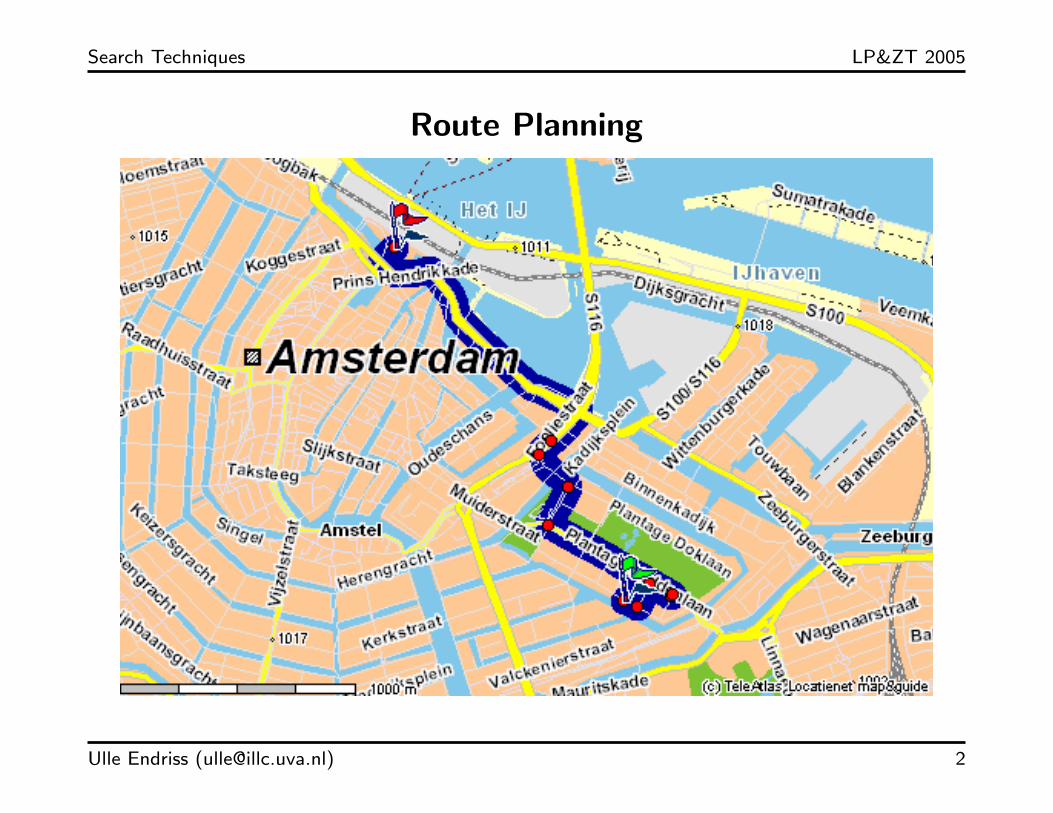
Robot Navigation

Source: http://www.ics.forth.gr/cvrl/


http://www.ics.forth.gr/cvrl/


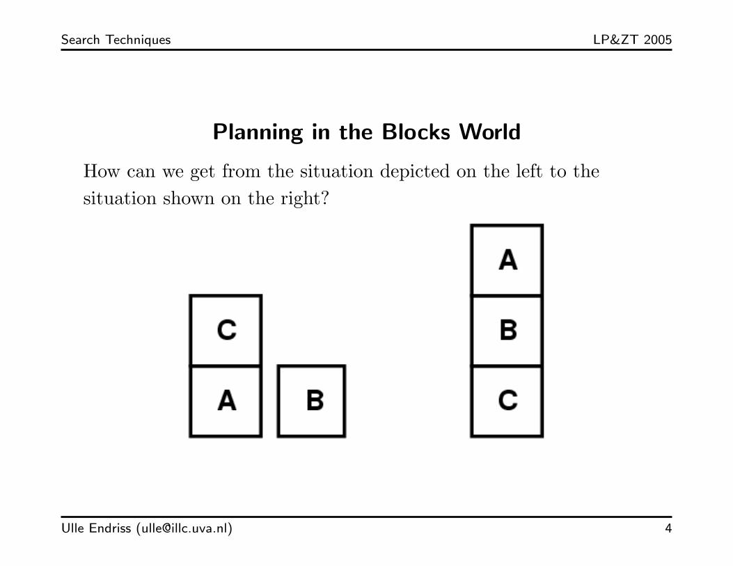
Planning in the Blocks World

How can we get from the situation depicted on the left to thesituation shown on the right?



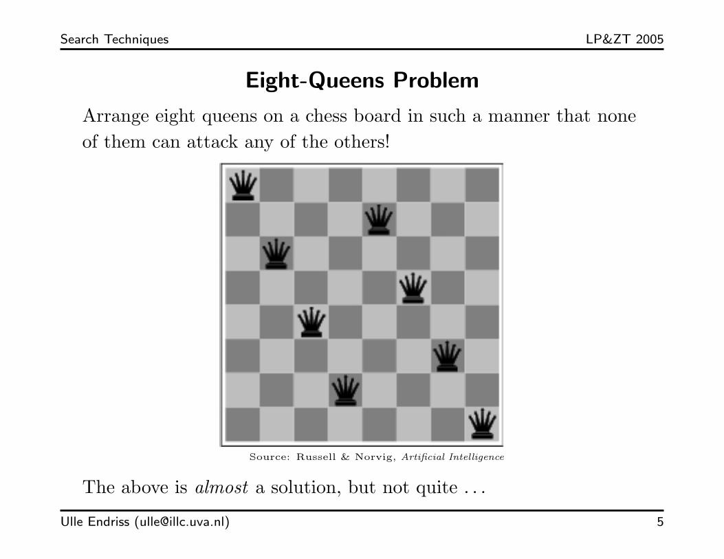
Eight-Queens Problem

Arrange eight queens on a chess board in such a manner that noneof them can attack any of the others!

Source: Russell & Norvig, Artificial Intelligence

The above is almost a solution, but not quite . . .



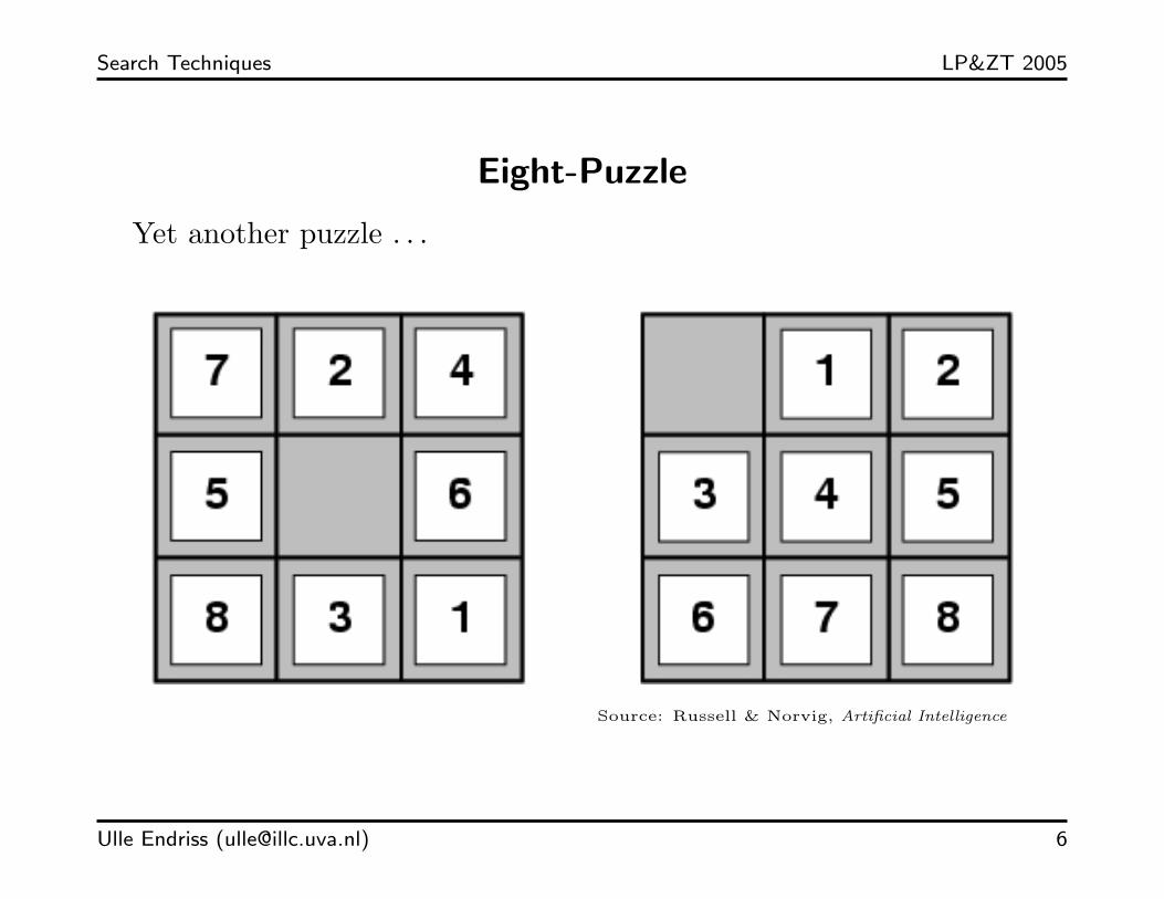
Eight-Puzzle

Yet another puzzle . . .




Search and Optimisation Problems

All these problems have got a common structure:

• We are faced with an initial situation and we would like toachieve a certain goal.

• At any point in time we have different simple actions availableto us (e.g. “turn left” vs. “turn right”). Executing a particularsequence of such actions may or may not achieve the goal.

• Search is the process of inspecting several such sequences andchoosing one that achieves the goal.

• For some applications, each sequence of actions may beassociated with a certain cost. A search problem where we aimnot only at reaching our goal but also at doing so at minimalcost is an optimisation problem.



The State-Space Representation

• State space: What are the possible states? Examples:

– Route planning: position on the map

– Blocks World: configuration of blocks

A concrete problem must also specify the initial state.

• Moves: What are legal moves between states? Examples:

– Turning 45◦ to the right could be a legal move for a robot.

– Putting block A on top of block B is not a legal move ifblock C is currently on top of A.

• Goal state: When have we found a solution? Example:

– Route planning: position = “Plantage Muidergracht 24”

• Cost function: How costly is a given move? Example:

– Route planning: The cost of moving from position X toposition Y could be the distance between the two.



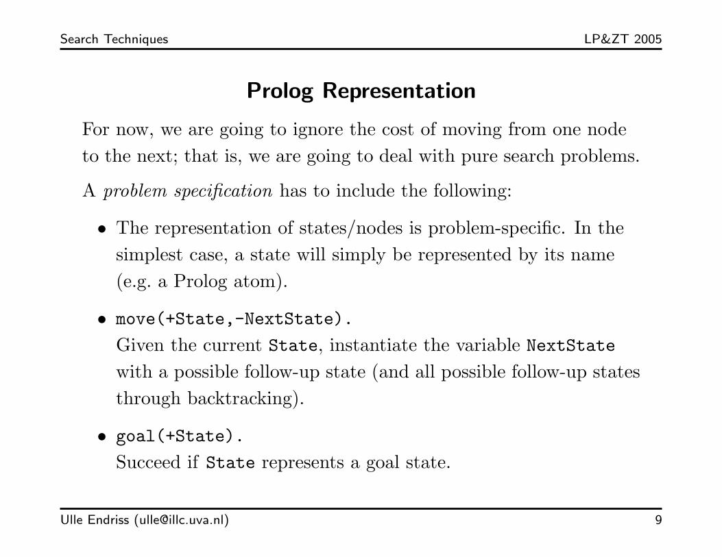
Prolog Representation

For now, we are going to ignore the cost of moving from one nodeto the next; that is, we are going to deal with pure search problems.

A problem specification has to include the following:

• The representation of states/nodes is problem-specific. In thesimplest case, a state will simply be represented by its name(e.g. a Prolog atom).

• move(+State,-NextState).

Given the current State, instantiate the variable NextState

with a possible follow-up state (and all possible follow-up statesthrough backtracking).

• goal(+State).

Succeed if State represents a goal state.



Example: Representing the Blocks World

• State representation: We use a list of three lists with the atomsa, b, and c somewhere in these lists. Each sublist represents astack. The first element in a sublist is the top block. The orderof the sublists in the main list does not matter. Example:

[ [c,a], [b], [] ]

• Possible moves: You can move the top block of any stack ontoany other stack:

move(Stacks, NewStacks) :-

select([Top|Stack1], Stacks, Rest),

select(Stack2, Rest, OtherStacks),

NewStacks = [Stack1,[Top|Stack2]|OtherStacks].

• Goal state: We assume our goal is always to get a stack with a

on top of b on top of c (other goals are, of course, possible):

goal(Stacks) :- member([a,b,c], Stacks).



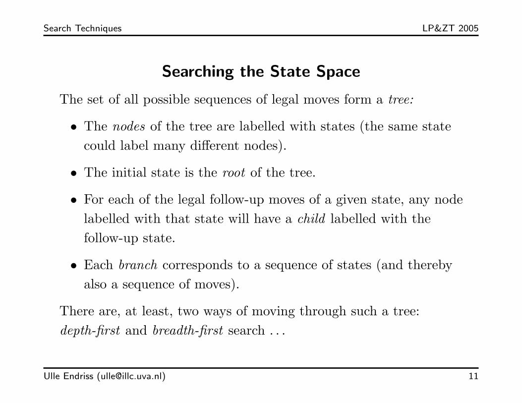
Searching the State Space

The set of all possible sequences of legal moves form a tree:

• The nodes of the tree are labelled with states (the same statecould label many different nodes).

• The initial state is the root of the tree.

• For each of the legal follow-up moves of a given state, any nodelabelled with that state will have a child labelled with thefollow-up state.

• Each branch corresponds to a sequence of states (and therebyalso a sequence of moves).

There are, at least, two ways of moving through such a tree:depth-first and breadth-first search . . .



Depth-first Search

In depth-first search, we start with the root node and completelyexplore the descendants of a node before exploring its siblings (andsiblings are explored in a left-to-right fashion).

Depth-first traversal: A → B → D → E → C → F → G

Implementing depth-first search in Prolog is very easy, becauseProlog itself uses depth-first search during backtracking.



Depth-first Search in Prolog

We are going to define a “user interface” like the following for eachof our search algorithms:

solve_depthfirst(Node, [Node|Path]) :-

depthfirst(Node, Path).

Next the actual algorithm: Stop if the current Node is a goal state;otherwise move to the NextNode and continue to search. Collectthe nodes that have been visited in Path.

depthfirst(Node, []) :-

goal(Node).

depthfirst(Node, [NextNode|Path]) :-

move(Node, NextNode),

depthfirst(NextNode, Path).



Testing: Blocks World

It’s working pretty well for some problem instances . . .

?- solve_depthfirst([[c,b,a],[],[]], Plan).

Plan = [[[c,b,a], [], []],

[[b,a], [c], []],

[[a], [b,c], []],

[[], [a,b,c], []]]

Yes

. . . but not for others . . .

?- solve_depthfirst([[c,a],[b],[]], Plan).

ERROR: Out of local stack



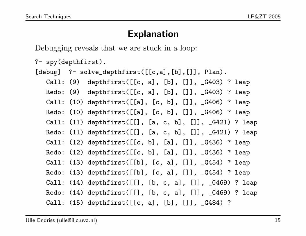
Explanation

Debugging reveals that we are stuck in a loop:

?- spy(depthfirst).

[debug] ?- solve_depthfirst([[c,a],[b],[]], Plan).

Call: (9) depthfirst([[c, a], [b], []], _G403) ? leap

Redo: (9) depthfirst([[c, a], [b], []], _G403) ? leap

Call: (10) depthfirst([[a], [c, b], []], _G406) ? leap

Redo: (10) depthfirst([[a], [c, b], []], _G406) ? leap

Call: (11) depthfirst([[], [a, c, b], []], _G421) ? leap

Redo: (11) depthfirst([[], [a, c, b], []], _G421) ? leap

Call: (12) depthfirst([[c, b], [a], []], _G436) ? leap

Redo: (12) depthfirst([[c, b], [a], []], _G436) ? leap

Call: (13) depthfirst([[b], [c, a], []], _G454) ? leap

Redo: (13) depthfirst([[b], [c, a], []], _G454) ? leap

Call: (14) depthfirst([[], [b, c, a], []], _G469) ? leap

Redo: (14) depthfirst([[], [b, c, a], []], _G469) ? leap

Call: (15) depthfirst([[c, a], [b], []], _G484) ?



Cycle Detection

The solution is simple: we need to disallow any moves that wouldresult in a loop. That is, if the next state is already present in theset of nodes visited so far, choose another follow-up state instead.

From now on we are going to use the following “wrapper” aroundthe move/2 predicate defined by the application:

move_cyclefree(Visited, Node, NextNode) :-

move(Node, NextNode),

\+ member(NextNode, Visited).

Here, the first argument should be instantiated with the list ofnodes visited already.

But note that we cannot just replace move/2 by move_cyclefree/3

in depthfirst/2, because Visited is not available where needed.



Cycle-free Depth-first Search in Prolog

Now the nodes will be collected as we go along, so we have toreverse the list of nodes in the end:

solve_depthfirst_cyclefree(Node, Path) :-

depthfirst_cyclefree([Node], Node, RevPath),

reverse(RevPath, Path).

The first argument is an accumulator collecting the nodes visited sofar; the second argument is the current node; and the thirdargument will be instantiated with the solution path (which equalsthe accumulator once we’ve hit a goal node):

depthfirst_cyclefree(Visited, Node, Visited) :-

goal(Node).

depthfirst_cyclefree(Visited, Node, Path) :-

move_cyclefree(Visited, Node, NextNode),

depthfirst_cyclefree([NextNode|Visited], NextNode, Path).



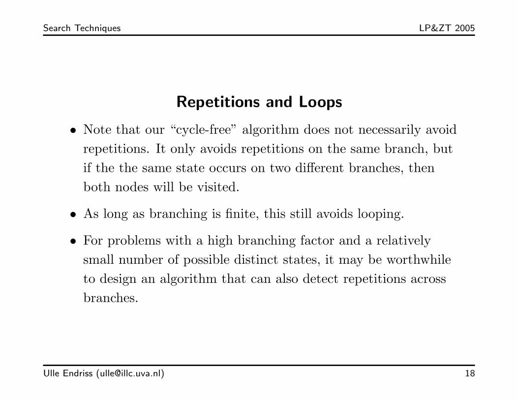
Repetitions and Loops

• Note that our “cycle-free” algorithm does not necessarily avoidrepetitions. It only avoids repetitions on the same branch, butif the the same state occurs on two different branches, thenboth nodes will be visited.

• As long as branching is finite, this still avoids looping.

• For problems with a high branching factor and a relativelysmall number of possible distinct states, it may be worthwhileto design an algorithm that can also detect repetitions acrossbranches.



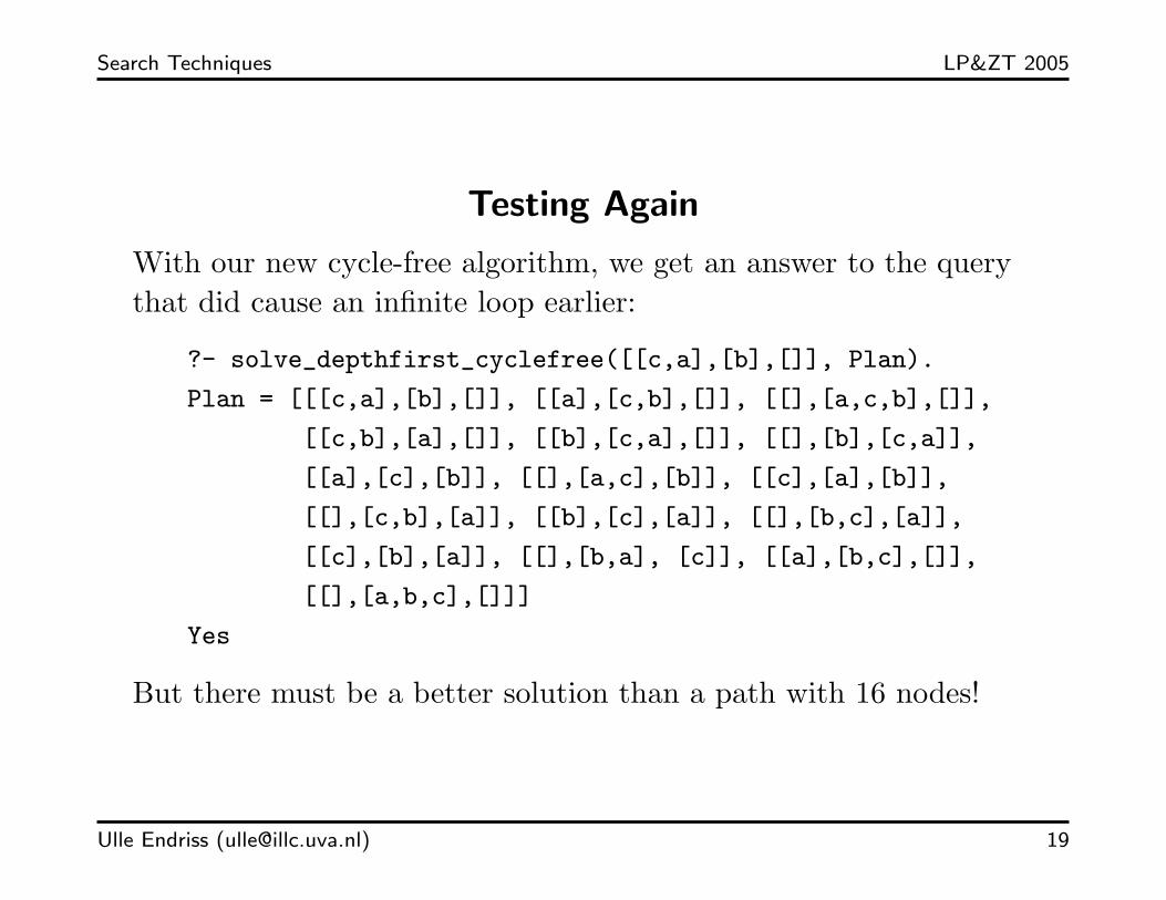
Testing Again

With our new cycle-free algorithm, we get an answer to the querythat did cause an infinite loop earlier:

?- solve_depthfirst_cyclefree([[c,a],[b],[]], Plan).

Plan = [[[c,a],[b],[]], [[a],[c,b],[]], [[],[a,c,b],[]],

[[c,b],[a],[]], [[b],[c,a],[]], [[],[b],[c,a]],

[[a],[c],[b]], [[],[a,c],[b]], [[c],[a],[b]],

[[],[c,b],[a]], [[b],[c],[a]], [[],[b,c],[a]],

[[c],[b],[a]], [[],[b,a], [c]], [[a],[b,c],[]],

[[],[a,b,c],[]]]

Yes

But there must be a better solution than a path with 16 nodes!



Restricting Search to Short Paths

• A possible solution to our problem of getting an unnecessarilylong solution path is to restrict search to paths of “acceptable”length.

• The idea is to stop expanding the current branch once it hasreached a certain maximal depth (the bound) and to move onto the next branch.

• Of course, like this we may miss some solutions further downthe current path. On the other hand, we increase chances offinding a short solution on another branch within a reasonableamount of time.



Depth-bounded Depth-first Search in Prolog

The program is basically the same as for cycle-free depth-firstsearch. We have one additional argument, the Bound, to bespecified by the user.

solve_depthfirst_bound(Bound, Node, Path) :-

depthfirst_bound(Bound, [Node], Node, RevPath),


depthfirst_bound(_, Visited, Node, Visited) :-

goal(Node).

depthfirst_bound(Bound, Visited, Node, Path) :-

Bound > 0,

move_cyclefree(Visited, Node, NextNode),

NewBound is Bound - 1,

depthfirst_bound(NewBound, [NextNode|Visited], NextNode, Path).



Testing Again

Now we can generate a short plan for our Blocks World problem, atleast if we can guess a suitable value for the bound required asinput to the depth-bounded depth-first search algorithm:

?- solve_depthfirst_bound(2, [[c,a],[b],[]], Plan).

No

?- solve_depthfirst_bound(3, [[c,a],[b],[]], Plan).

Plan = [[[c,a], [b], []],

[[a], [c], [b]],

[[], [b, c], [a]],

[[], [a, b, c], []]]

Yes



Complexity Analysis

• It is important to understand the complexity of an algorithm.

– Time complexity: How much time will it take to compute asolution to the problem?

– Space complexity: How much memory do we need to do so?

• We may be interested in both a worst-case and an average-casecomplexity analysis.

– Worst-case analysis: How much time/memory will thealgorithm require in the worst case?

– Average-case analysis: How much time/memory will thealgorithm require on average?

• It is typically extremely difficult to give a formal average-caseanalysis that is theoretically sound. Experimental studies usingreal-world data are often the only way.; Here we are only going to attempt a worst-case analysis.



Time Complexity of Depth-first Search

• As there can be infinite loops, in the worst case, the simpledepth-first algorithm will never stop. So we are going toanalyse depth-bounded depth-first search instead.

• Let dmax be the maximal depth allowed. (If we happen to knowthat no branch in the tree can be longer than dmax , then ouranalysis will also apply to the other two depth-first algorithms.)

• For simplicity, assume that for every possible state there areexactly b possible follow-up states. That is, b is the branchingfactor of the search tree.



Time Complexity of Depth-first Search (cont.)

• What is the worst case?

In the worst case, every branch has length dmax (or more) andthe only node labelled with a goal state is the last node on therightmost branch. Hence, depth-first search will visit all thenodes in the tree (up to depth dmax ) before finding a solution.

• So how many nodes are there in a tree of height dmax withbranching factor b?

⇒ 1 + b + b2 + b3 + · · ·+ bdmax

Example: b = 2 and dmax = 2

1+21+22 = 22+1−1 = 7



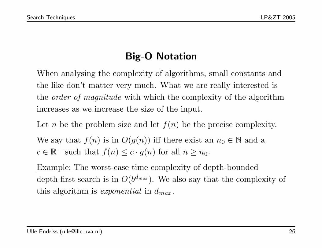
Big-O Notation

When analysing the complexity of algorithms, small constants andthe like don’t matter very much. What we are really interested isthe order of magnitude with which the complexity of the algorithmincreases as we increase the size of the input.

Let n be the problem size and let f(n) be the precise complexity.

We say that f(n) is in O(g(n)) iff there exist an n0 ∈ N and ac ∈ R+ such that f(n) ≤ c · g(n) for all n ≥ n0.

Example: The worst-case time complexity of depth-boundeddepth-first search is in O(bdmax ). We also say that the complexity ofthis algorithm is exponential in dmax .



Exponential Complexity

In general, in Computer Science, anything exponential is consideredbad news. Indeed, our simple search techniques will usually notwork very well (or at all) for larger problem instances.

Suppose the branching factor is b = 4 and suppose it takes us1 millisecond to check one node. What kind of depth bound wouldbe feasible to use in depth-first search?

Depth Nodes Time

2 21 0.021 seconds

5 1365 1.365 seconds

10 1398101 23.3 minutes

15 1431655765 16.6 days

20 1466015503701 46.5 years



Space Complexity of Depth-first Search

The good news is that depth-first search is very efficient in view ofits memory requirements:

• At any point in time, we only need to keep the path from theroot to the current node in memory, and —depending on theexact implementation— possibly also all the sibling nodes foreach of the nodes in that path.

• The length of the path is at most dmax+1 and each of the nodeson the path will have at most b−1 siblings left to consider.

• Hence, the worst-case space complexity is O(b · dmax ).That is, the complexity is linear in dmax .

In fact, because Prolog uses backtracking, sibling nodes do notneed to be kept in memory explicitly. Therefore, space complexityeven reduces to O(dmax ).



Breadth-first Search

The problem with (unbounded) depth-first search is that we mayget lost in an infinite branch, while there could be another shortbranch leading to a solution.

The problem with depth-bounded depth-first search is that it canbe difficult to correctly estimate a good value for the bound.

Such problems can be overcome by using breadth-first search, wherewe explore (right-hand) siblings before children.

Breadth-first traversal: A → B → C → D → E → F → G



Breadth-first Search: Implementation Difficulties

How do we keep track of which nodes we have already visited andhow do we identify the next node to go to?

Recall that for depth-first search, in theory, we had to keep thecurrent branch in memory, together with all the sibling nodes ofthe nodes on that branch.

Because of the way backtracking works, in Prolog we actually onlyhad to keep track of the current node (Prolog keeps thecorresponding path on its internal recursion stack).

For breadth-first search, we are going to have to take care of thememory management by ourselves.



Breadth-first Search: Implementation Idea

The algorithm will maintain a list of the currently active paths.

Each round of the algorithm running consists of three steps:

(1) Remove the first path from the list of paths.

(2) Generate a new path for every possible follow-up state of thestate labelling the last node in the selected path.

(3) Append the list of newly generated paths to the end of the listof paths (to ensure paths are really being visited inbreadth-first order).



Breadth-first Search in Prolog

The usual “user interface” takes care of initialising the list of activepaths and of reversing the solution path in the end:

solve_breadthfirst(Node, Path) :-

breadthfirst([[Node]], RevPath),


And here is the actual algorithm:

breadthfirst([[Node|Path]|_], [Node|Path]) :-

goal(Node).

breadthfirst([Path|Paths], SolutionPath) :-

expand_breadthfirst(Path, ExpPaths),

append(Paths, ExpPaths, NewPaths),

breadthfirst(NewPaths, SolutionPath).



Expanding Branches

We still need to implement expand_breadthfirst/2 . . .

Given a Path (represented in reverse order), the predicate shouldgenerate the list of expanded paths we get by making a single movefrom the last Node in the input path.

expand_breadthfirst([Node|Path], ExpPaths) :-

findall([NewNode,Node|Path],

move_cyclefree(Path,Node,NewNode),

ExpPaths).



Example

We are now able to find the shortest possible plan for our BlocksWorld scenario, without having to guess a suitable bound first:

?- solve_breadthfirst([[c,a],[b],[]], Plan).

Plan = [[[c,a], [b], []],

[[a], [c], [b]],

[[], [b,c], [a]],

[[], [a,b,c], []]]

Yes



Completeness and Optimality

Some good news about breadth-first search:

• Breadth-first search guarantees completeness: if there exists asolution it will be found eventually.

• Breadth-first search also guarantees optimality: the firstsolution returned will be as short as possible.

(Remark: This interpretation of optimality assumes that everymove has got a cost of 1. With real cost functions it doesbecome a little more involved.)

Recall that depth-first search does not ensure either completenessor optimality.



Complexity Analysis of Breadth-first Search

Time complexity: In the worst case, we have to search through theentire tree for any search algorithm. As both depth-first andbreadth-first search visit each node exactly once, time complexitywill be the same.

Let d be the the depth of the first solution and let b be thebranching factor (again, assumed to be constant for simplicity).Then worst-case time complexity is O(bd).

Space complexity: Big difference; now we have to store every pathvisited before, while for depth-first we only had to keep a singlebranch in memory. Hence, space complexity is also O(bd).

So there is a trade-off between memory-requirements on the onehand and completeness/optimality considerations on the other.



Best of Both Worlds

We would like an algorithm that, like breadth-first search, isguaranteed (1) to visit every node on the tree eventually and (2) toreturn the shortest possible solution, but with (3) the favourablememory requirements of a depth-first algorithm.

Observation: Depth-bounded depth-first search almost fits the bill.The only problem is that we may choose the bound either

• too low (losing completeness by stopping early) or

• too high (becoming too similar to normal depth-first with thedanger of getting lost in a single deep branch).

Idea: Run depth-bounded depth-first search again and again, withincreasing values for the bound!

This approach is called iterative deepening . . .



Iterative Deepening

We can specify the iterative deepening algorithm as follows:

(1) Set n to 0.

(2) Run depth-bounded depth-first search with bound n.

(3) Stop and return answer in case of success;increment n by 1 and go back to (2) otherwise.

However, in Prolog we can implement the same algorithm also in amore compact manner . . .



Finding a Path from A to B

A central idea in our implementation of iterative deepening inProlog will be to provide a predicate that can compute a path ofmoves from a given start node to some end node.

path(Node, Node, [Node]).

path(FirstNode, LastNode, [LastNode|Path]) :-

path(FirstNode, PenultimateNode, Path),

move_cyclefree(Path, PenultimateNode, LastNode).



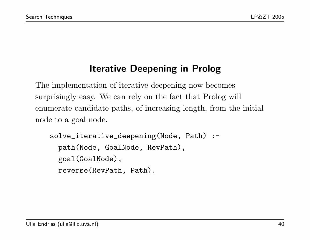
Iterative Deepening in Prolog

The implementation of iterative deepening now becomessurprisingly easy. We can rely on the fact that Prolog willenumerate candidate paths, of increasing length, from the initialnode to a goal node.

solve_iterative_deepening(Node, Path) :-

path(Node, GoalNode, RevPath),

goal(GoalNode),




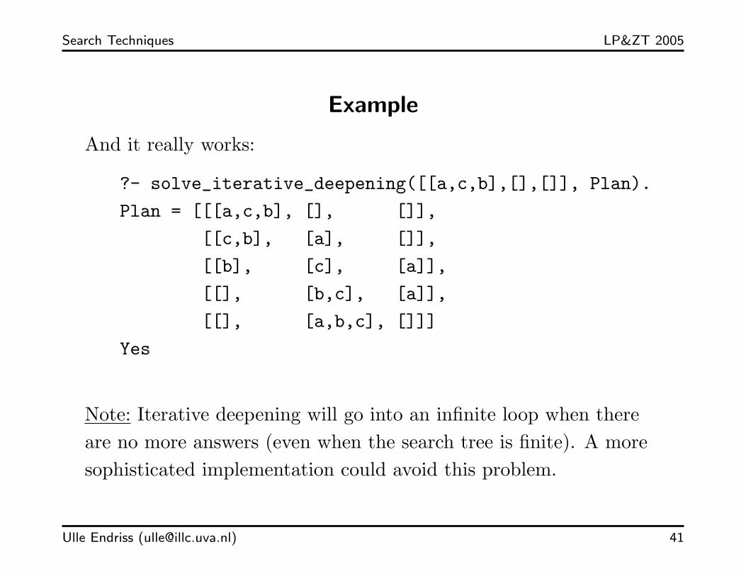
Example

And it really works:

?- solve_iterative_deepening([[a,c,b],[],[]], Plan).

Plan = [[[a,c,b], [], []],

[[c,b], [a], []],

[[b], [c], [a]],

[[], [b,c], [a]],

[[], [a,b,c], []]]

Yes

Note: Iterative deepening will go into an infinite loop when thereare no more answers (even when the search tree is finite). A moresophisticated implementation could avoid this problem.



Complexity Analysis of Iterative Deepening

Space complexity: As for depth-first search, at any moment in timewe only keep a single path in memory ; O(d).

Time complexity: This seems worse than for the other algorithms,because the same nodes will get generated again and again.

However, time complexity is of the same order of magnitude asbefore. If we add the complexities for depth-bounded depth-firstsearch for maximal depths 0, 1, . . . , d (somewhat abusing notation),we still end up with O(bd):

O(b0) + O(b1) + O(b2) + · · ·+ O(bd) = O(bd)

In practice, memory issues are often the greater problem, anditerative deepening is typically the best of the (uninformed) searchalgorithms we have considered so far.



Summary: Uninformed Search

We have introduced the following general-purpose algorithms:

• Depth-first search:

– Simple version: solve_depthfirst/2

– Cycle-free version: solve_depthfirst_cyclefree/2

– Depth-bounded version: solve_depthfirst_bound/3

• Breadth-first search: solve_breadthfirst/2

• Iterative deepening: solve_iterative_deepening/2

These algorithms (and their implementations, as given on theseslides) are applicable to any problem that can be formalised usingthe state-space approach. The Blocks World has just been anexample!

Next we are going to see how to formalise a second (very different)problem domain.



Recall the Eight-Queens Problem

Arrange eight queens on a chess board in such a manner that noneof them can attack any of the others!


The above is almost a solution, but not quite . . .



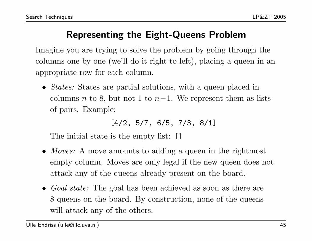
Representing the Eight-Queens Problem

Imagine you are trying to solve the problem by going through thecolumns one by one (we’ll do it right-to-left), placing a queen in anappropriate row for each column.

• States: States are partial solutions, with a queen placed incolumns n to 8, but not 1 to n−1. We represent them as listsof pairs. Example:

[4/2, 5/7, 6/5, 7/3, 8/1]

The initial state is the empty list: []

• Moves: A move amounts to adding a queen in the rightmostempty column. Moves are only legal if the new queen does notattack any of the queens already present on the board.

• Goal state: The goal has been achieved as soon as there are8 queens on the board. By construction, none of the queenswill attack any of the others.



Specifying the Attack-Relation

The predicate noattack/2 succeeds if the queen given in the firstargument position does not attack any of the queens in the listgiven as the second argument.

noattack(_, []).

noattack(X/Y, [X1/Y1|Queens]) :-

X =\= X1, % not in same column

Y =\= Y1, % not in same row

Y1-Y =\= X1-X, % not on ascending diagonal

Y1-Y =\= X-X1, % not on descending diagonal

noattack(X/Y, Queens).

Examples:

?- noattack(3/4, [1/8,2/6]). ?- noattack(2/7, [1/8]).

Yes No



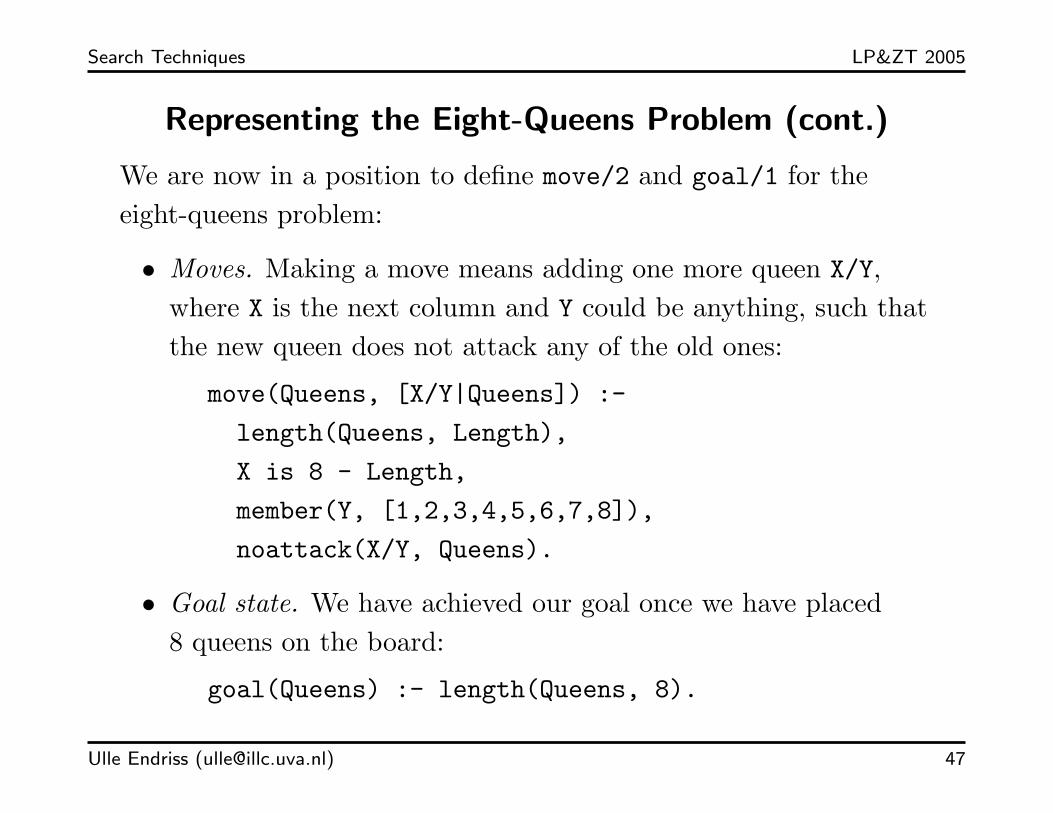
Representing the Eight-Queens Problem (cont.)

We are now in a position to define move/2 and goal/1 for theeight-queens problem:

• Moves. Making a move means adding one more queen X/Y,where X is the next column and Y could be anything, such thatthe new queen does not attack any of the old ones:

move(Queens, [X/Y|Queens]) :-

length(Queens, Length),

X is 8 - Length,

member(Y, [1,2,3,4,5,6,7,8]),

noattack(X/Y, Queens).

• Goal state. We have achieved our goal once we have placed8 queens on the board:

goal(Queens) :- length(Queens, 8).



Solution

What is special about the eight-queens problem (or rather ourformalisation thereof) is that there are no cycles or infinite branchesin the search tree. Therefore, all of our search algorithms will work.

Here’s the (first) solution found by the basic depth-first algorithm:

?- solve_depthfirst([], Path), last(Path, Solution).

Path = [[], [8/1], [7/5, 8/1], [6/8, 7/5, 8/1], ...]

Solution = [1/4, 2/2, 3/7, 4/3, 5/6, 6/8, 7/5, 8/1]

Yes

Note that here we are not actually interested in the path to thefinal state, but only the final state itself (hence the use of last/2).



Heuristic-guided Search

• Our complexity analysis of the various basic search algorithmshas shown that they are unlikely to produce results for slightlymore complex problems than we have considered here.

• In general, there is no way around this problem. In practice,however, good heuristics that tell us which part of the searchtree to explore next, can often help to find solutions also forlarger problem instances.

• In this final chapter on search techniques for AI, we are goingto discuss one such heuristic, which leads to the well-knownA* algorithm.



Optimisation Problems

• From now on, we are going to consider optimisation problems(rather than simple search problems as before). Now everymove is associated with a cost and we are interested in asolution path that minimises the overall cost.

• We are going to use a predicate move/3 instead of move/2. Thethird argument is used to return the cost of an individual move.



Best-first Search and Heuristic Functions

• For both depth-first and breadth-first search, which node in thesearch tree will be considered next only depends on thestructure of the tree.

• The rationale in best-first search is to expand those paths nextthat seem the most “promising”. Making this vague idea ofwhat may be promising precise means defining heuristics.

• We fix heuristics by means of a heuristic function h that is usedto estimate the “distance” of the current node n to a goal node:

h(n) = estimated cost from node n to a goal node

Of course, the definition of h is highly application-dependent.In the route-planning domain, for instance, we could use thestraight-line distance to the goal location. For the eight-puzzle,we might use the number of misplaced tiles.



Best-first Search Algorithms

There are of course many different ways of defining a heuristicfunction h. But there are also different ways of using h to decidewhich path to expand next; which gives rise to different best-firstsearch algorithms.

One option is greedy best-first search:

• expand a path with an end node n such that h(n) is minimal

Breadth-first and depth-first search may also be seen as specialcases of best-first search (which do not use h at all):

• Breadth-first: expand the (leftmost of the) shortest path(s)

• Depth-first: expand the (leftmost of the) longest path(s)



Example: Greedy Best-first Search

Greedy best-first search means always trying to continue with thenode that seems closest to the goal. This will work sometimes, butnot all of the time:

Clearly, greedy best-first search is not optimal. Like depth-firstsearch, it is also not complete.



The A* Algorithm

The central idea in the so-called A* algorithm is to guide best-firstsearch both by

• the estimate to the goal as given by the heuristic function h and

• the cost of the path developed so far.

Let n be a node, g(n) the cost of moving from the initial node to n

along the current path, and h(n) the estimated cost of reaching agoal node from n. Define f(n) as follows:

f(n) = g(n) + h(n)

This is the estimated cost of the cheapest path through n leadingfrom the initial node to a goal node. A* is the best-first searchalgorithm that always expands a node n such that f(n) is minimal.



A* in Prolog

On the following slides, we give an implementation of A* in Prolog.Users of this algorithm will have to implement the followingapplication-dependent predicates themselves:

• move(+State,-NextState,-Cost).

Given the current State, instantiate the variable NextState

with a possible follow-up state and the variable Cost with theassociated cost (all possible follow-up states should getgenerated through backtracking).

• goal(+State).

Succeed if State represents a goal state.

• estimate(+State,-Estimate).

Given a State, instantiate the variable Estimate with anestimate of the cost of reaching a goal state. This predicateimplements the heuristic function.



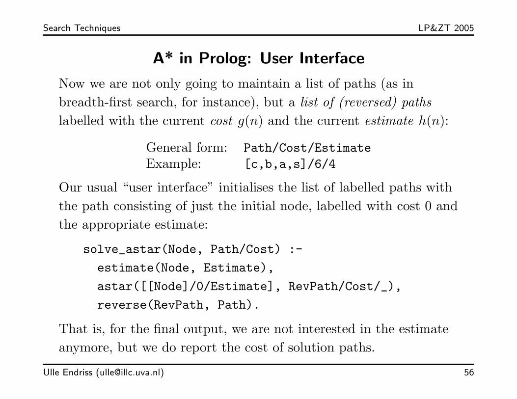
A* in Prolog: User Interface

Now we are not only going to maintain a list of paths (as inbreadth-first search, for instance), but a list of (reversed) pathslabelled with the current cost g(n) and the current estimate h(n):

General form: Path/Cost/EstimateExample: [c,b,a,s]/6/4

Our usual “user interface” initialises the list of labelled paths withthe path consisting of just the initial node, labelled with cost 0 andthe appropriate estimate:

solve_astar(Node, Path/Cost) :-

estimate(Node, Estimate),

astar([[Node]/0/Estimate], RevPath/Cost/_),


That is, for the final output, we are not interested in the estimateanymore, but we do report the cost of solution paths.



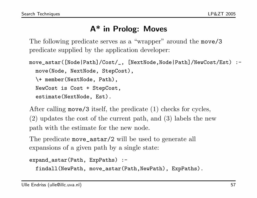
A* in Prolog: Moves

The following predicate serves as a “wrapper” around the move/3predicate supplied by the application developer:

move_astar([Node|Path]/Cost/_, [NextNode,Node|Path]/NewCost/Est) :-

move(Node, NextNode, StepCost),

\+ member(NextNode, Path),

NewCost is Cost + StepCost,

estimate(NextNode, Est).

After calling move/3 itself, the predicate (1) checks for cycles,(2) updates the cost of the current path, and (3) labels the newpath with the estimate for the new node.

The predicate move_astar/2 will be used to generate allexpansions of a given path by a single state:

expand_astar(Path, ExpPaths) :-

findall(NewPath, move_astar(Path,NewPath), ExpPaths).



A* in Prolog: Getting the Best Path

The following predicate implements the search strategy of A*: froma list of labelled paths, we select one that minimises the sum of thecurrent cost and the current estimate.

get_best([Path], Path) :- !.

get_best([Path1/Cost1/Est1,_/Cost2/Est2|Paths], BestPath) :-

Cost1 + Est1 =< Cost2 + Est2, !,

get_best([Path1/Cost1/Est1|Paths], BestPath).

get_best([_|Paths], BestPath) :-

get_best(Paths, BestPath).

Remark: Implementing a different best-first search algorithm onlyinvolves changing get_best/2; the rest can stay the same.



A* in Prolog: Main Algorithm

Stop in case the best path ends in a goal node:

astar(Paths, Path) :-

get_best(Paths, Path),

Path = [Node|_]/_/_,

goal(Node).

Otherwise, extract the best path, generate all its expansions, andcontinue with the union of the remaining and the expanded paths:

astar(Paths, SolutionPath) :-

get_best(Paths, BestPath),

select(BestPath, Paths, OtherPaths),

expand_astar(BestPath, ExpPaths),

append(OtherPaths, ExpPaths, NewPaths),

astar(NewPaths, SolutionPath).



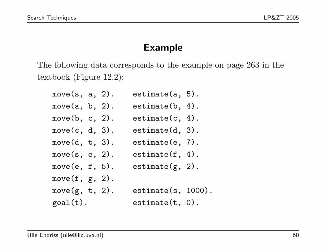
Example

The following data corresponds to the example on page 263 in thetextbook (Figure 12.2):

move(s, a, 2). estimate(a, 5).

move(a, b, 2). estimate(b, 4).

move(b, c, 2). estimate(c, 4).

move(c, d, 3). estimate(d, 3).

move(d, t, 3). estimate(e, 7).

move(s, e, 2). estimate(f, 4).

move(e, f, 5). estimate(g, 2).

move(f, g, 2).

move(g, t, 2). estimate(s, 1000).

goal(t). estimate(t, 0).



Example (cont.)

If we run A* on this problem specification, we first obtain theoptimal solution path and then one more alternative path:

?- solve_astar(s, Path).

Path = [s, e, f, g, t]/11 ;

Path = [s, a, b, c, d, t]/12 ;

No



Debugging

We can use debugging to reconstruct the working of A* for thisexample (trace edited for readability):

?- spy(expand_astar).

Yes

[debug] ?- solve_astar(s, Path).

Call: (10) expand_astar([s]/0/1000, _L233) ? leap

Call: (11) expand_astar([a, s]/2/5, _L266) ? leap

Call: (12) expand_astar([b, a, s]/4/4, _L299) ? leap

Call: (13) expand_astar([e, s]/2/7, _L353) ? leap

Call: (14) expand_astar([c, b, a, s]/6/4, _L386) ? leap

Call: (15) expand_astar([f, e, s]/7/4, _L419) ? leap

Call: (16) expand_astar([g, f, e, s]/9/2, _L452) ? leap

Path = [s, e, f, g, t]/11

Yes



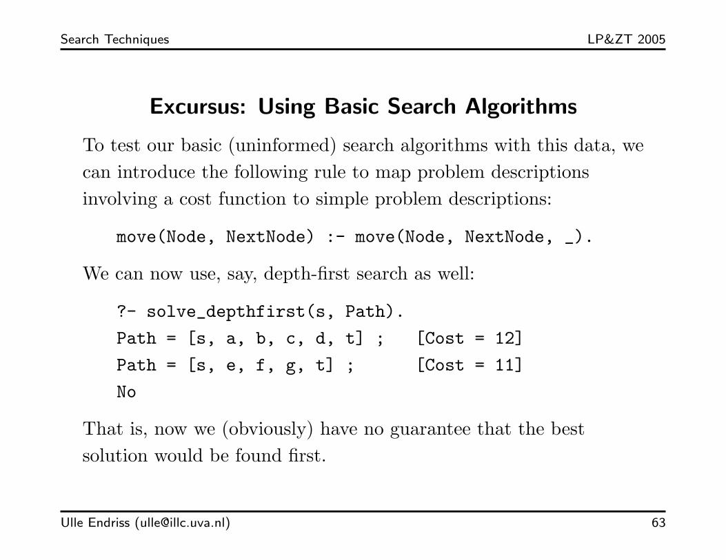
Excursus: Using Basic Search Algorithms

To test our basic (uninformed) search algorithms with this data, wecan introduce the following rule to map problem descriptionsinvolving a cost function to simple problem descriptions:

move(Node, NextNode) :- move(Node, NextNode, _).

We can now use, say, depth-first search as well:

?- solve_depthfirst(s, Path).

Path = [s, a, b, c, d, t] ; [Cost = 12]

Path = [s, e, f, g, t] ; [Cost = 11]

No

That is, now we (obviously) have no guarantee that the bestsolution would be found first.



Properties of A*

A heuristic function h is called admissible iff h(n) is never morethan the actual cost of the best path from n to a goal node.

An important theoretical result is the following:

A* with an admissible heuristic function guaranteesoptimality, i.e. the first solution found has minimal cost.

Proof: Let n be a node on an optimal solution path and let n′ be anon-optimal goal node. We need to show that A* will always pick n

over n′. Let c∗ be the cost of the optimal solution. We get(1) f(n′) = g(n′) + h(n′) = g(n′) + 0 > c∗ and, due to admissibilityof h, (2) f(n) = g(n) + h(n) ≤ c∗. Hence, f(n) < f(n′), q.e.d.

Also note that A* with any heuristic function guaranteescompleteness, i.e. if a solution exists it will be found eventually.



Admissible Heuristic Functions

How do we choose a “good” admissible heuristic function?

Two general examples:

• The trivial heuristic function h0(n) = 0 is admissible.

It guarantees optimality, but it is of no help whatsoever infocussing the search; so using h0 is not efficient.

• The perfect heuristic function h∗, mapping n to the actual costof the optimal path from n to a goal node, is also admissible.

This function would lead us straight to the best solution(but, of course, we don’t know what h∗ is!).

Finding a good heuristic function is a serious research problem . . .



Recall the Route Planning Problem



Examples for Admissible Heuristics

For the route planning domain, we could think of the followingheuristic functions:

• Let h1(n) be the straight-line distance to the goal location.

This is an admissible heuristic, because no solution path willever be shorter than the straight-line connection.

• Let h2(n) be h1(n) + 20%.

An intuitive justification would be that there are no completelystraight streets anyway, so this would be a better estimate thanh1(n). Indeed, h2 may often work better than h1, but it is notgenerally admissible (because there may be two locationsconnected by an almost straight street). So h2 does notguarantee optimality.



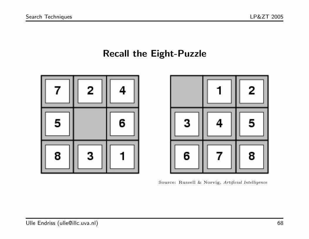
Recall the Eight-Puzzle




Examples for Admissible Heuristics (cont.)

For the eight-puzzle, the following heuristic functions come to mind:

• Let h3(n) be the number of misplaced tiles (so h3(n) will be anumber between 0 and 8).

This is clearly a lower bound for the number of moves to thegoal state; so it is also an admissible heuristic.

• Assume we could freely move tiles along the vertical andhorizontal, without regard for the other tiles. Let h4(n) be thenumber we get when we count the 1-step moves required to getto the goal configuration under this assumption.

This is also an admissible heuristic, because in reality we willalways need at least h4(n) moves (and typically more, becauseother tiles will be in the way). Furthermore, h4 is better thanh3, because we have h3(n) ≤ h4(n) for all nodes n.



Complexity Analysis of A*

Both worst-case time and space complexity are exponential in thedepth of the search tree (like breadth-first search): in the worstcase, we still have to visit all the nodes on the tree and ultimatelykeep the full tree in memory.

The reason why A* usually works much better than basicbreadth-first search anyway, is that the heuristic function willtypically allow us to get to the solution much faster.

Remark: In practice, our implementation of the basic A* algorithmmay not perform that well, because of the high memoryrequirements. In the textbook there is a discussion of alternativealgorithms that consume less space (at the expense of taking moretime, which is typically quite acceptable).



Summary: Best-first Search with A*

• Heuristics can be used to guide a search algorithm in a largesearch space. The central idea of best-first search is to expandthe path that seems most promising.

• There are different ways of defining a heuristic function h toestimate how far off the goal a given node is; and there aredifferent ways of using h to decide which node is “best”.

• In the A* algorithm, the node n minimising the sum of the costg(n) to reach the current node n and the estimate h(n) of thecost to reach a goal node from n is chosen for expansion.

• A heuristic function h is called admissible iff it neverover-estimates the true cost of reaching a goal node.

• If h is an admissible heuristic function, then A* guaranteesthat an optimal solution will be found (first).



Conclusion: Search Techniques for AI

• Distinguish uninformed and heuristic-guided search techniques:

– The former are very general concepts and applicable topretty much any computing problem you can think of(though maybe not in exactly the form presented here).

– The latter is a true AI theme: defining a really goodheuristic function arguably endows your system with adegree of “intelligence”. Good heuristics can lead to verypowerful search algorithms.

• You should have learned that there is a general “pattern” toboth the implementation of these algorithms and to the(state-space) representation of problems to do with search.

• You should have learned that analysing the complexity ofalgorithms is important; and you should have gained someinsight into how that works.


search techniques for artiﬁcial intelligencecsatol/log_funk/prolog/slides/7-search.pdfsearch...

Documents