search dynamics in consumer choice under time pressure: an eye

American Economic Review 101 (April 2011): 900–926http://www.aeaweb.org/articles.php?doi=10.1257/aer.101.2.900

900

Consider the problem of a consumer in a modern supermarket. The typical store sells more than 40,000 items, and in many product categories it offers hundreds of options (for a recent review see Simona Botti and Sheena S. Iyengar 2006). The typical consumer is also time constrained and cannot afford to spend too much time making each selection. To solve this decision problem consumers need to per-form a dynamic search over the set of feasible items under conditions of extreme time pressure and choice overload. This gives rise to several basic questions which are studied in this paper: (i) What are the computational processes deployed by consumers during the search and decision processes, and to what extent are they compatible with standard economic search models? (ii) How do the processes, and their performance, change with the number of options? (iii) Do the computational processes exhibit systematic biases that can be exploited by sellers to manipulate their choices?

We study these questions by setting up an experimental version of the consumer’s supermarket problem. Hungry subjects are presented with sets of 4, 9, or 16 familiar snack items (e.g., Snickers candy bars and Lay’s chips) and are asked to make a choice within three seconds. Items are displayed using pictures of the actual pack-ages of items. Besides choices and reaction times, the entire process of visual search is recorded using eye tracking.

A key goal of the study, made feasible by the use of eye tracking, is to open the black box of decision making and to study the computational processes used by subjects to make these types of choices (Martjin C. Willemsen and Eric J. Johnson 2009). We propose and compare three competing models of the computational processes used to make these fast decisions. All of the models are straightforward variations of well-known dynamic search models in economics (Boyan Jovanovic 1979; John J. McCall 1970). The first model assumes optimal search with zero search costs, which implies that subjects search for the maximum amount of items possible before making a choice, and then choose the best-seen item. The second model assumes satisficing, which implies that subjects search until they have found

Search Dynamics in Consumer Choice under Time Pressure: An Eye-Tracking Study

By Elena Reutskaja, Rosemarie Nagel, Colin F. Camerer, and Antonio Rangel*

* Reutskaja: Marketing Department, IESE Business School, Barcelona Campus, Avenida Pearson, 21, 08034 Barcelona, Spain (e-mail: [email protected]); Nagel: Department of Economics and Business, Universitat Pompeu Fabra and ICREA, Ramon Trias Fargas, 25-27, Barcelona 08005, Spain (e-mail: [email protected]); Camerer: Computational and Neural Systems and Division of the Humanities and Social Sciences, 1200 East California Blvd., Pasadena, CA 91125 (e-mail: [email protected]); Rangel: Computational and Neural Systems and Division of the Humanities and Social Sciences, 1200 East California Blvd., Pasadena, CA 91125 (e-mail: [email protected]). The order of authors is listed using natural science conventions. Financial support from HFSP (RN and CFC), the Moore Foundation (AR and CFC), the Spanish Ministry of Education (RN, SEJ2005-08391), the Barcelona CREA program (RN), Barcelona Graduate School of Economics (RN), and the Generalitat de Catalunya (RN) is gratefully acknowledged.

901REutskAjA Et Al.: sEARch DynAmics in consumER choicEVol. 101 no. 2

a sufficiently good item, or run out of time. The third model is a hybrid in which subjects search for a random amount of time, which depends on the value of the encountered items, and then choose the best-seen item.

We find that subjects are good at optimizing within the set of items that they see during the search process (the “seen set”), and that the search process is random with respect to value, so that items with higher value are not more likely to be noticed. The results also show that subjects use a stopping rule to terminate the search process that is qualitatively consistent with the hybrid model, but not with the satisficing or optimal search models. Furthermore, a calibration of the hybrid model provides a good quantitative match of several features of the observed data.

Our experimental design also allows us to test if the choice process is subject to display effects, so that the probability that an item is selected depends on its loca-tion on the display. We find that subjects exhibit a bias to look first and more often to items that are placed in certain regions of the display, which they also end up choosing more often.

Looking at the computational process generating choices is unusual in neoclas-sical economics. Traditional economists generally build models and interpret their data using the concept of revealed preference, which is silent about the actual com-putational processes used to make choices. This is true even in some behavioral economics models (e.g., prospect theory or quasi-hyperbolic-discounting) in which subjects are assumed to act as if they were maximizing an objective function, but in which the computational process generating the choices is not spelled out.1 Although this view has worked extremely well in many applications, there are domains, such as the problem of consumer decision making under time pressure, in which under-standing the underlying computational process is central to understanding the eco-nomics of the problem.

To see why, note that sellers spend billions of dollars trying to manipulate in-store choice. Knowledge of the algorithm that consumers use to make their fast choices is essential to being able to make predictions about the qualitative and quantita-tive effects of such practices as well as about their effects on consumer well being. Understanding the computational process can make new predictions about how vari-ables such as physical display, visual features, attention, exogeneous initial condi-tions, and memory can affect choices (Pierre Chandon et al. 2008).

This study builds on previous literatures from economics, marketing, and psy-chology. In economics, several groups have used eye tracking to study the computa-tional process used to make strategic decisions. Using a simpler technology than eye tracking, called MouseLab, (Camerer et al. 1993; Johnson et al. 2002) showed that the pattern of offers in alternating-offer bargaining experiments could be explained to a large extent by a failure to carry out full “backward induction,” since in many trials subjects did not look ahead to see what amounts would be available if initial offers were rejected. Camerer and Johnson (2004) established a related result for the case of “forward induction.” Miguel Costa-Gomes, Vincent P. Crawford, and Bruno Broseta (2001) used this same technique to measure steps of strategic thinking in

1 Some behavioral economics models are more explicit about computational processes, such as “cognitive hierarchy” and level-k models in game theory (Camerer 2003; Nagel 1995) and similarity-based models (Ariel Rubinstein 1988).

902 thE AmERicAn Economic REViEW APRil 2011

normal-form games (see also Costa-Gomes and Crawford 2006). Xavier Gabaix et al. (2006) used MouseLab to investigate the pattern of information acquisition used in complex multiattribute and multialternative choice. Isabelle Brocas et al. (2009) showed how limited strategic thinking in private information games can be associated with information acquisition. Using modern camera-based eye-tracking techniques, Daniel T. Knoepfle, Joseph Tao-yi Wang, and Camerer (2009) and Wang, Michael Spezio, and Camerer (2010) studied strategic information transmis-sion and found that a combination of lookup information and pupil dilation could help predict an unobservable private information state. More closely related to this study, Andrew Caplin and Mark Dean (2009) and Caplin, Dean, and Daniel Martin (forthcoming) have collected nonstandard behavioral data (in the form of interim choices which are continually updated) to try to identify some of the properties of the dynamic search algorithm used by consumers facing complex choices.

Several studies in marketing have used eye tracking to study how consumers choose products from different types of displays. J. Edward Russo and Larry D. Rosen (1975) started this literature by studying how subjects moved their eyes while making hypothetical choices out of six-item text-based descriptions of cars. They argued, as we do in this paper, that the pattern of eye fixations provides a window into the computational process used to make choices (see also Russo and France Leclerc 1994). Using more modern eye-tracking techniques, Ralf Van der Lans (2006) studied how subjects locate brands within a display, but the experi-ment included no choice. The closest study to the current paper is by Chandon et al. (2008) who look at the hypothetical choices of consumers facing familiar consumer products out of large choice sets without time pressure (their average overall reac-tion time is 25 seconds). They find, as we do, that visual attention plays a critical role in choice.

Several additional studies in marketing have also used eye tracking to study which features of advertisements receive most attention, but they involve no real deci-sion making for actual products (Gerald L. Lohse 1997; Lizzie Maughan, Sergei Gutnikov, and Rob Stevens 2007; Rik Pieters, Edward Rosbergen, and Michael Wedel 1999; Pieters and Wedel 2004). Some of these studies have found, as we do, that display location impacts fixations. Note, however, that none of these papers has studied real choice under time pressure and option overload. For a comprehensive review of the literature see Russo (2010).

This paper also builds on the early ideas of John W. Payne, James R. Bettman, and Johnson (1993) who used MouseLab to show individuals who are under high cognitive strain (perhaps due to information overload), or under time pressure, shift to simpler computational models (see also Bettman, Mary Frances Luce, and Payne 1998; A. John Maule and Anne C. Edland 1997). Our computational “bounded rationality” model also allows the possibility of a similar shift across choice set sizes. However, both the details of the model and the eye-tracking evidence that we present are new to this literature.

Finally, our approach is related to the “choice overload” literature in psychology. Those studies, like ours, investigate choices from sets of different sizes, but the items are typically more complex and less familiar (such as jams, investments, or pictures). These studies typically find that for large sets subjects often do not choose at all, postponing choice (Iyengar, Gur Huberman, and Wei Jiang 2004; Iyengar


and Mark R. Lepper 2000). One study shows that subjects report disliking small and large choice sets and preference for intermediate sets (Elena Reutskaja and Robin M. Hogarth 2009). Another study shows neural activity consistent with both increased cognitive load and overall devaluation for sets that are too large (Reutskaja et al. 2009). Our results appear to be fundamentally different, since subjects always make a choice.

The paper is organized as follows. Section I describes the experimental design. Section II describes the three competing models of the choice process. Section III provides a qualitative test of the key assumptions of the three models. Section IV shows that an appropriately calibrated version of the hybrid model also matches the data quantitatively. Section V explores the impact of the size of the choice set on the properties and performance of the choice process. Section VI presents the evidence on the presence of display effects. Section VII concludes.

I. Experimental Design

The aim of this laboratory experiment was to study economic decision making under conditions of extreme time pressure and overload.

Forty-one Caltech undergraduates participated in the study. Individuals were excluded if they had a history of eating disorders, had dieted in the past year, were vegetarian, disliked junk food, or were pregnant. Subjects received $35 for participating and provided informed consent. Participants were asked to eat and then fast for three hours prior to the experiment. No deception was used.

At the beginning of the instruction period participants were told that they would have to stay in the lab for an additional 30 mins at the end of the experiment. During this time they were allowed to eat the food item that they chose in a randomly selected trial according to the rules described below, but no other foods or drinks were allowed. Subjects made choices out of a set of 70 popular snacks such as candy bars (e.g., Snickers Bar) and potato chips (e.g., Lay’s).

Participants performed two tasks: (i) a liking-rating task, and (ii) a choice task.During the liking-rating task subjects had to answer the question “How much

would you like to eat this item at the end of the experiment?” on a scale of −5 (“not at all”) to 5 (“very much”), with 0 denoting indifference. Liking ratings are the only measure of item value used in this study, but previous research has found that liking ratings are very highly correlated with dollar willingness-to-pay for similar foods (Todd A. Hare, Camerer, and Rangel 2009; Hare et al. 2008; Hilke Plassmann, John O’Doherty, and Rangel 2007), as well as charities (Hare et al. 2010).

The liking-rating trials started with a 1s central fixation cross, followed by a 3s presentation of a picture of the item to be rated. Pictures were 400 × 300 pixels in size and showed both the package and the food. Then subjects entered their liking-ratings at their own pace using the keyboard. The items were shown in random order. There was a 1s inter-trial interval with an empty screen.

During the choice tasks subjects were shown 75 choice sets consisting of either 4, 9, or 16 snack food items (25 of each of the three set sizes). The items were pre-sented simultaneously in a computer screen (see Figure 1 for examples). The sets were presented in such a way that the average distance among items was equalized across set sizes. The identity and location of items was fully randomized. The order


of the choice sets was also randomized. No identical items were present in the same choice set.

Before the appearance of each set the subject was shown a black screen with a central white fixation cross. The subject had to maintain continuous fixation on the cross for two seconds before the choice set was displayed. This was enforced with an eye tracker, and it was implemented to eliminate anticipatory eye movements.

Each choice set was presented for a maximum of 3s. Participants, however, could make their choices in less than three seconds. Two seconds into the choice period subjects heard a beep indicating that they had exactly one second left until the choice set would vanish. Subjects indicated their choice by pressing the keyboard while fix-ating on an item. Prior to making actual choices, subjects went through 12 practice rounds to familiarize themselves with the equipment and procedure.

At the end of the experiment a trial was selected at random and the subjects were given the chance to eat the food that they chose in that trial. Subjects were penalized with a loss of $3 if they failed to make a choice within three seconds in the selected trial.

The entire choice process was monitored with an eye tracker (Eye-tracker model: Tobii 1750, Tobii Technology, Sweden) that recorded the positioning of the eye gazes on the screen every 20 ms with an approximate resolution of 0.25 square inches.

After the experiment subjects answered a questionnaire regarding their snack-ing habits. The experiment, including the instruction period, lasted an average of 60 minutes, including the 30 minutes that a participant had to spend in an adjacent room while eating his food.

II. Models

In this section we propose three competing models of the computational process used by the subjects to make the choices: (i) an optimal search model with zero search costs, (ii) a satisficing search model, and (iii) a hybrid search model.

The models and analyses below use the following notions of visual attention: fixa-tion, initial fixation, and refixation. A fixation occurs when a subject looks at an item for a continuous period of time (50 ms or more). Note that during a fixation subjects might look at different parts of the picture. These small eye movements within a fixation are known as microfixations and are ignored in the study. A fixation on an item is an initial fixation if that is the first time that the subject fixates on that item during the trial. Otherwise it is called a refixation.

Figure 1. Examples of Screenshots for the Set Sizes 4, 9, and 16

Set size 4 Set size 9 Set size 16


All of the models assume that the choice process has two phases: (i) an initial search phase, and (ii) a final choice phase. All of the models also assume that subjects need to fixate on the items during the initial search phase in order to learn their value, and that the initial search process is random with respect to value. More precisely, the models assume that subjects begin the choice process every trial by searching through the choice set without replacement using a sequence of distinct fixations. Let F t denote the identity of the item seen in fixation t. We assume that during each fixa-tion t the brain computes several variables: (i) A value V t to the item that it is looking at; (ii) a cached value ct equal to the value of the best seen item at the end of fixation t; and (iii) the set of items that have been seen so far st. Note that the probability of fixat-ing on a particular item during the initial stage is independent of its absolute or rela-tive value. We assume that c0 = −5, which is the lowest possible rating for an item.

At some point the initial search phase ends, and the choice process enters a final choice phase. The models differ on how the initial search is stopped and on how the final choice is made.

The optimal search model with zero costs assumes that subjects look at as many items as possible during the initial phase, subject to the constraint of having enough time left to make a final fixation to select the favorite seen item (which might be different from the last item seen). Let

_ t be the maximum search time

for the initial phase (i.e., after this time no new search fixations are initiated). When the initial search process ends the subject makes a choice out of the set of items that he has seen (call it

_ s , which might be a strict subset of the entire choice

set). We assume that the subject is able to select the best item in the seen set with probability q, which might depend on the set size, and with probability 1 − q he randomizes over all items in the choice set (regardless of whether or not they have been previously seen) with equal probability.

The satisficing model assumes that subjects search until either _ t seconds have

elapsed, or the subject has found an item with a reservation value of _ V or higher,

whatever occurs first. In the former case a probabilistic choice over the seen set is made as described above. Otherwise the item with value

_ V or higher is selected.

The reservation value might depend on the set size. Note that the satisficing model makes two strong predictions. First, any choices that involve a refixation should be to an item of value less than

_ V (since an item of value

_ V would immediately be

chosen after initially fixating on it). Second, any choices made prior to _ t should

generate a value of _ V or higher.

The hybrid model incorporates elements of both models. It assumes that at the end of every new fixation of the initial search phase the subjects decide to stop the search process, with probability pt, or continue the search, with probability 1 − pt . We assume that pt increases with the time elapsed within the trial as well as with the cached value ct , and that it equals 1 when all of the items in the choice set have been seen, or after

_ t seconds have passed. After the initial search phase ends the subjects

probabilistically select an item out of the seen set using the same soft-maximization process described above.

Note several things about this class of models.First, the models are closely related. They all assume that subjects search through

the feasible set at random during an initial search phase, and that when they are done searching they select the best item that was seen during the search, up to some noise.


Second, the models differ on the stopping rule for the initial search phase. The optimal model assumes that subjects search until they have seen everything or until they run out of time. The satisficing model assumes that subjects search until they find an item with a value at or above a reservation value

_ V , or until they run out of

time. The hybrid model assumes that the initial search process terminates with a probability that increases on the number of items that have been seen and on the value of the best seen item. The optimal model can be viewed as a special case of the hybrid model in which the probability of terminating the search process depends highly nonlinearly on the number of seen items and on the elapsed time, but not on the value of the items that have been seen. The satisficing model can also be viewed as a special case of the hybrid model in which the probability of terminating the search process depends strongly on the value of the best seen item, and in which elapsed time matters only when the subject has run out of search time.

Third, it is straightforward to see that the number of fixations plays a crucial role in this model: on average subjects make good choices when they see a lot of items, but not when they see few items. This naturally raises the question of fixation duration. We assume that fixation duration is approximately fixed and independent of values and set size. This assumption is based on the idea that there is a biological limitation to how fast the brain can fixate on an item and extract its value, and that subjects move near that threshold when making decisions under extreme time pressure.

Fourth, although the initial search is assumed to be random with respect to value, this does not rule out the possibility that it might be influenced by other variables such as the location of an item in the display, or its location relative to previously seen items.

Fifth, we assume that when subjects reach the final choice phase, they use a prob-abilistic choice rule over the set of seen items (except for the case of satisficing when an item of sufficiently high value was found during the initial search).2

Sixth, the value assigned to an item is assumed to be independent of the length of the fixation. This is a reasonable approximation because the items are familiar and fixation times did not vary significantly across items. Note, however, that previ-ous work has shown that fixation times can affect valuation and choices (K. Carrie Armel, Aurelie Beaumel, and Rangel 2008; Armel and Rangel 2008; Ian Krajbich, Armel, and Rangel 2008).

Seventh, we have assumed that there is perfect memory about the value of previ-ously seen items as well as their locations. This implies that the only purpose of a refixation (going back to a previously seen item) is to select the previously seen item that is thought to be best, but not to see it again to recall a value. This “perfect recall” assumption is unlikely to hold in more complicated choice. Interestingly, the extreme time pressure in our experiments might actually help recall in the sense that a rapid choice time makes short-term memory more effective. People might see less, but remember more, than if they had more time. It is even conceivable that an extension of the model proposed, which includes memory decay, would predict

2 There is early (Duncan R. Luce 1959), extensive (David W. Harless and Camerer 1994; John D. Hey and Chris Orme 1994), statistical (Nathaniel T. Wilcox 2008), and biological (Rangel 2008) support for this type of “soft maximization.”


that allowing longer choice times hurts choice quality (if the bad effects of memory decay outweigh the benefits from having more time to look or deliberate).

III. Model Tests and Comparisons

In this section we use the behavioral and eye-tracking data to test the key assump-tions of the models, and thus to test between them. The section is organized into three parts. First we test the assumption, common to the three models, that there is an initial search phase during which subjects sample items at random without replacement. Second, we test the assumption, also common to the three models, that after the initial search phase ends subjects choose the best seen item, up to some noise. Third, we compare the stopping rules that describe the three different models with the actual stopping process used by the subjects.

A. Random initial search Process

The three proposed models assume that subjects engage in a sequential search phase during which items are sampled at random, without replacement, and inde-pendent of value. Figure 2 provides a test of this assumption. For every trial we define the initial search phase to be the search process prior to the first refixation (if any). Then we compute the efficiency of each fixation (relative to the entire choice set) in this initial search phase. The efficiency of item i in set s is given by

e(i | s) = V i − mean{ V j | j ∈ s }

___ max{ V j | j ∈ s } − mean{ V j | j ∈ s } ,

where V k denotes the value of the items, as measured by the initial liking rating col-lected in the experiment.3 The resulting mean fixation efficiencies for each set size are shown in Figure 2. Two aspects are worth highlighting. First, average fixation efficiency does not improve with lookup order which, consistent with the assump-tion of random search order, means that subjects are not able to fixate on better items as the initial search progresses. Second, the average efficiency of the fixations are slightly above zero (9.7 percent for n = 4, p < 0.0000, 6.7 percent for n = 9, p < 0.0000, 10 percent for n = 16, p < 0.0000, t-tests4). This implies that subjects are able to do some coarse form of evaluation and preselection with their peripheral vision in order to direct their gaze to above average items, but the effect is quantita-tively small. Thus, the evidence presented in Figure 2 is roughly consistent with the assumption of initial random search.

3 Note several things about this measure. First, efficiency equals zero for an item with mean value, it is equal to one for items with the maximum value in the set, and is negative when subjects choose an item with less than mean value. Second, the concept can be used to answer several questions of interest: What is the efficiency of the chosen item out of the feasible set? What is the efficiency of the chosen item out of the set of items that was seen during the initial search phase? What is the efficiency of a fixation relative to the entire set of items, or to the set of items that have been previously seen? Third, since the statistic is not defined for sets in which the mean and the maximum set value are identical, in all of the analysis below we exclude the very few trials (< 5 percent) in which this is the case.

4 All t-tests reported in the paper are computed over the subject’s means.


B. optimal choice within the seen set

Another common assumption among the models is that after the initial phase has terminated subjects select the best item out of the same set with a fixed probability q, and with probability 1 − q they randomize over the whole choice set. The only exception is for the satisficing model, which assumes that if the initial search phase is terminated by identifying an item above the reservation value, then that item is selected immediately. Note that, in all cases, the choice is made either by selecting the last seen item (in which case there are no refixations), or by refixating to the chosen item (in which case there is one refixation). Figure 3 provides a test of these components of the models.

Figure 3 panel A shows the frequency with which the best item seen in the initial search phase is eventually chosen. The mean frequencies are 76 percent for n = 4, 73 percent for n = 9, and 69 percent for n = 16 (all pairwise t-tests are significant at p < 0.003). Figure 7 panel C shows that the mean number of fixations is 3.3 for n = 4, 4.9 for n = 9, and 5.5 for n = 16. Given this, if subjects were choosing at random over the seen set, the mean frequencies with which the best choice is selected would be 30 percent, 20 percent, and 18 percent, respectively. A simple t-test for each case rejects this alternative hypothesis at p < 0.0000 in all cases. We can then conclude that the subjects most often choose the best seen item, although the likelihood is slightly decreasing with set size.

Figure 3 panels B and C investigate in more detail why the probability of selecting the best item is decreasing with the number of options. Figure 3 panel B shows the

Figure 2. Mean Efficiency of Initial Fixations by the Order of the Fixations (new fixations only, excludes refixations)

1 2 3 4 5 6 7

Fixation number

8

Fix

atio

n ef

ficie

ncy

−0.4

−0.2

0.0

0.2

0.4

N = 16

N = 9

N = 4


probability that the best item is selected as a function of how many trials before the end of the initial search phase it was seen. The effect of this lag is strong: the probabil-ity of selecting the best item is 83 percent when it was seen on the final initial fixation but only 37.6 percent when it was seen four fixations before (pairwise paired t-test p < 0.0000). This suggests that in some of the trials subjects exhibit imperfect recall about the location of high-value items, and that the problem is exacerbated with the number of options that have been seen during the initial search phase. This is likely due to working memory limitations that are more likely to appear in larger choice sets when more options are seen (see Figure 7, panel C) before making a choice.

Figure 3. Tests of the Optimization Algorithm

notes: Panel A: Probability that the best item seen during the initial fixation phase is eventually chosen as a func-tion of set size. Panel B: Probability that the best item seen during the initial fixation phase is eventually chosen as a function of the number of fixations since it was seen. Panel C: Histograms showing the frequencies of different number of refixations as a function of set size. Panel D: Probability that the trial ends with no refixations as a func-tion of the value of the currently seen item minus the cached value at the end of the previous fixation. Error bars denote SEM.

Pro

b be

st it

em in

see

n se

t cho

sen

0.0

0.2

0.4

0.6

0.8

1.0

4 9 16Set size

Pro

b be

st it

em in

see

n se

t cho

sen

0.0

0.2

0.4

0.6

0.8

1.0

0 1 2 3 4

Number fixations since best last seen

Panel A Panel B

Panel C Panel D

Pro

b N

O r

efix

atio

ns

0.0

0.2

0.4

0.6

0.8

1.0

4

Current value MINUS previous cached value0−5−10

N = 4 N = 9 N = 16

Number of refixations

Per

cent

0.0

0.2

0.4

0.6

0.8

1.0

0.0 1.0 2.0 3.0

N = 4

N = 9

N = 16

0.0

0.2

0.4

0.6

0.8

1.0

0.0 1.0 2.0 3.0

0.0

0.2

0.4

0.6

0.8

1.0

0.0 1.0 2.0 3.0


Figure 3 panel C shows the distribution of the number of refixations for different set sizes. During the choice phase subjects mostly deploy either zero refixations (because they choose the last item seen in the initial search phase) or one refixation. The percentage of trials in which there are two or more refixations are 28 percent for n = 4 and 16, and 23 percent for n = 9. The existence of these additional refix-ations means that the data are only approximately consistent with the simple models described above, which suggests the possibility that in some trials subjects might remember the best item but not its location, and thus that they might have to refixate multiple times to find it.

Figure 3 panel D tests another aspect of the subjects’ ability to optimize over the seen set. The models assume that the probability that the last seen item is chosen (in which case there are no refixations) should increase with Vt − ct−1. The figure tests this prediction by plotting the probability that the last item seen in the initial phase is chosen as a function of this variable. The data show that subjects’ choices are quite sensitive to the difference between these two variables, which suggests that they are proficient at comparing current and cached values. This is important because it suggests that the occasional inability to optimize over the seen set identified above might be driven by an inability to recall or find the location of the best item in the crowded display within the available time constraints, rather than by an inability to know what the value of the cached item is.

C. tests of the stopping Rules

A critical difference between the three models has to do with the stopping rule determining the end of the initial search phase. In this section we sequentially com-pare the performance of the stopping rules for the three models.

The optimal search model assumes that the search ends when the subject has either seen all of the items, or run out of time, whichever happens first. Figure 4 panel A provides a test of this stopping rule. It shows the probability that the current fixation terminates the initial search phase as a function of how many items have been seen so far (i.e., the fixation number). The graph shows that the probability increases with the fixation number for all set sizes, although the effect decreases with set size. The termination probability increases gradually from about 0 percent for the first initial fixation to 87 percent by the fourth fixation in the case of n = 4, 77 percent by the eighth fixation for the case of n = 9, and 50 percent by the eighth fixation for the case of n = 16 (linear slope=18 percent for n = 4, 9.1 percent for n = 9, and 6.8 percent for n = 16). Importantly, the probability of termination increases con-tinuously with the fixation number, and thus with the time elapsed on the trial, and does not exhibit a discontinuous increase after a certain number of fixations (which serves as a proxy of the elapsed time) have passed. This constitutes strong evidence against the optimal search model with zero costs since in that case the probability of terminating the initial search phase should be zero early on and then discontinuously jump to 100 percent after the all of available time has been used (or all of the items have been seen).

The satisficing model assumes that the search ends when the subject finds an item with reservation value

_ V , or when he runs out of time, whichever happens first.

Figure 4 panel B provides a test of this stopping rule. That model assumes that the


initial search phase ends when an item with reservation value of V * or higher is seen, or when the subject runs out of time. Importantly, the model predicts that the probability of a given initial fixation’s being the last one should be approximately zero for low values of the currently seen item, and then discontinuously jump to 100 percent when the value exceeds V * . Figure 4 panel B shows that this is not the case: instead of a discontinuous jump at V * , the probability of terminating the initial search phase increases gradually with the value of the current fixation and never exceeds 50 percent. Importantly, only fixations that ended within the first 2,000 ms of the trial are included in this graph, which implies that subjects fail to follow a satisficing rule even when they have not run out of time. Furthermore, the fact that the stopping probability never exceeds 50 percent provides suggestive evidence for a tendency to explore as much of the feasible set as possible during the initial search phase, even when a very high value item has been seen.

0.0

0.2

0.4

Pro

b cu

rren

t fix

atio

n is

last

new

one

0.6

0.8

1.0 N = 16

N = 9

N = 4

1 2 3 4 5 6 7 8

Fixation number Value current fixation

Panel A Panel B

Panel C

0.0

0.2

0.4

0.6

0.8

1.0

–4 –2 0 2 4

Pro

b cu

rren

t fix

atio

n is

last

fina

l cho

ice

Pro

b la

st in

itial

fixa

tion

0.0

0.2

0.4

0.6

0.8

1.0

–4 –2 0 2 4

Cached value

N = 4

N = 9

N = 16

N = 4

N = 9

N = 16

Figure 4. Tests of the Stopping Rule

notes: Panel A: Probability that the current fixation ends the initial search phase as a function of fixation number. Panel B: Probability that the current fixation ends the initial search phase as a function of the value of the currently attended item. Panel C: Probability that the current fixation ends the initial search phase as a function of the cur-rent cached value.


The hybrid model assumes that subjects terminate the initial search phase with a probability that increases with the cached value and the elapsed time. Figure 4 panels A and C provide basic tests of this stopping rule. Figure 4 panel C shows that the probability of termination increases gradually from 0 percent for highly negative cached values to about 50 percent for highly positive cached values (linear slope = 6.4 percent for n = 4, 4.8 percent for n = 9, and 4.3 percent for n = 16). Figure 4 panel A shows that the termination probability increases gradually with the number of fixations.

IV. Quantitative Fit of the Hybrid Model

The tests in the previous section show that subjects’ behavior is qualitatively com-patible with the hybrid model, but not with the optimal search model with zero costs or with the satisficing model. In this section we investigate the ability of the hybrid model to explain the quantitative patterns of the data.

We performed the following calibration and simulation exercise for each set size separately. In each case the quantitative comparison between the simulated model and the actual data was performed by pooling together the data for all of the individuals into a single dataset. This was necessary because the model has a sizable degree of randomness, and there are only 25 observations for every subject and condition.

For each set size we carried out the following exercise 100 times. One hundred random trials were selected, and the model was simulated once for each of those data points. The simulated model assumed that the probability that a given initial fixation ends the initial search phase increases linearly with the cached value (with slope a) and with the elapsed time (with slope d). The simulated model also assumes that there is a constant probability q of selecting the best item out of the seen set, and that subjects fully randomize over the seen set otherwise. The resulting simulated models have only three free parameters: a, d, and q.

We use the results of the 100 runs to compute the mean and standard deviation for the simulated reaction time, total number of fixations, choice efficiency, and prob-ability of selecting the best-seen item, over the 100 exercises. Similar statistics were computed for the selected data. Fixation durations were simulated by sampling from the set of observed fixation durations.

The parameters of the model were calibrated as follows. First, for each set size q was given by the observed probability of selecting the best-seen item, as reported in Figure 3 panel A. Second, we randomly sampled a and d parameters from the set {0.0.1, … , 0.5} × {0, 0.00001, … , 0.0001} and simulated the model using the proce-dure described in the previous paragraph until a set of parameters was found for which two properties were satisfied: (P1) the confidence interval given by the mean simu-lated reaction time ± one standard deviation contained the mean of the data reaction times, and (P2) the confidence interval given by the mean simulated choice effi-ciency ± one standard deviation contained the mean of the data choice efficiencies. The convergence criterion was satisfied for the case of n = 9 and n = 16, but not for the case of n = 4. In that case we sampled 100 pairs of parameters and selected the pair with the smallest difference between the simulated and mean reaction times, out of the set of parameters that satisfied P2 described above.


Figure 5 depicts the results of the calibration exercise for the three set sizes and various statistics. Figure 5 panel A shows the results for reaction times. Each light-gray symbol represents the mean statistic for the 100 data and simulated points in each run of the exercise. The vertical bars represent the mean reaction time ( ± one standard deviation). The bars are plotted at the mean of the sampled data points. Panel B depicts the analogous exercise for the number of fixations, panel C for the realized choice efficiency, and panel D for the probability that the best item in the seen set is chosen. Overall, the figure shows that the simple hybrid model provides a good quantitative fit of the data. The main exception is the tendency of the simulated model to generate reaction times that were about 300 ms shorter than actual observed reaction times in the n = 4 set, and slight tendencies to overestimate the number of fixations and the chance of choosing the best seen item.

Panel A. rt Panel B. # fixations

2500

1000

0

Sim

ulat

ed

S

imul

ated

Sim

ulat

ed

S

imul

ated

0.8

0.4

0

0.8

0.4

0

10

8

6

4

2

0

Panel C. Efficiency Panel D. Prob best chosen

0 1000 2000 3000 0 2 4 6 8 10

0 0.4 0.8 0 0.4 0.8

Data Data

Data Data

N = 4

N = 9

N = 16

△+

N = 4

N = 9

N = 16

△+

N = 4

N = 9

N = 16

△+

N = 4

N = 9

N = 16

△+

Figure 5. Quantitative Fits of the Calibrated Model

notes: Panel A: Simulated versus actual reaction times (“rt”) by set size. Panel B: Simulated versus actual number of fixations per trial (“# fixations”) by set size. Panel C: Simulated versus actual choice efficiency (“efficiency”) by set size. Panel D: Simulated versus actual probability that the best item in the choice set is chosen (“prob best chosen”) by set size. Error bars denote SEM.


V. The Effect of Set Size

To the extent that the search parameters (e.g., fixation duration) remain constant across conditions, the hybrid model has implications for how the performance of the choice process changes with set size. This section explores these effects.

Consider the impact on the search process first. Figure 6 panel A describes the duration of the initial search phase (denoted by t * ) for the different set sizes. The mean duration of the initial phase was 1,138 ms for the case of n = 4, 1,571 ms for the case of n = 9, and 1,508 ms for the case of n = 16 (pairwise paired t-tests computed across subject means: p < 0.0000 for 4 versus 9, and 4 versus 16, n.s. for 9 versus 16). Figure 6 panel C provides a histogram of the t * statistic. Figure 6 panel B describes the total response time (which includes the duration of the initial search phase and the final choice phase) for each set size. The mean reaction times were 1,768 ms for the case of n = 4, 1,987 ms for the case of n = 9, and 2,056 ms for the case of n = 16.

Figure 7 panel A describes the mean fixation duration in each of the three cases (excluding refixations). The mean fixation duration was 373 ms for the case of n = 4, 359 ms for the case of n = 9, and 310 ms for the case of n = 16 (pairwise paired t-tests: p < 0.0000 for 4 versus 9, and 4 versus 16, n.s. for 4 versus 9). Figure 7 panel B shows the evolution of the mean fixation duration over the entire

Res

pons

e tim

e (m

s)

t*

3000

2500

2000

1500

1000

500

0

3000

2500

2000

1500

1000

500

0

Panel A

Panel C

Panel B

200

100

0

100

40

0

100

40

0

%

%

%

500 1,000 1,500 2,000 2,500 3,000

500 1,000 1,500 2,000 2,500 3,000

500 1,000 1,500 2,000 2,500 3,000

N = 4

N = 9

N = 6

t*

4 9 16Set size

4 9 16Set size

Figure 6. Effect of the Size on the Length of the Search Process

notes: Panel A: Average length of the initial search phase (denoted by t*) by set size. Panel B: Average response time by set size. Panel C: Distribution of initial search phase lengths by set size. Error bars denote SEM.


search process. Together, the two figures show that subjects have the ability to speed up the search process slightly in the presence of a large number of items, by decreasing the duration of the fixations by about 60 ms, but that subjects do not speed up the fixations as the trial advances (for example, when they are running out of time).

Figure 7 panel C shows that the average number of items seen in a trial increases with set size, from 3.3 items for the case on n = 4 to 5.5 items in the case of n = 16 (pairwise paired t-test, p < 0.0000). This is due to a combination of the shorter fixation durations and the longer search times for the case of n = 16. Note, however, that the set size increases faster than the subject’s ability to search the

# ite

ms

seen

F

ixat

ion

dura

tion

(ms)

400

300

200

100

0

Panel A Panel B

1 2 3 4 5 6 7 8 4 9 16Set size

400

300

200

100

0

8

6

4

3

04 9 16

Set size

4 9 16Set size

1.0

0.8

0.6

0.4

0.2

0.0

# ite

ms

seen

F

ixat

ion

dura

tion

4 9 16Set size

1.0

0.8

0.6

0.4

0.2

0.0

Panel E

Panel C Panel D

Pro

babl

y be

st it

em s

een

Figure 7. Effect of the Set Size on Fixation Durations and the Seen Set

notes: Panel A: Mean fixation duration by set size. Panel B: Mean fixation duration by fixation number and set size. Panel C: Mean number of items seen by set size. Panel D: Mean percentage of items seen by set size. Panel E: Probability that the best item in the choice set is seen by set size. Error bars denote SEM.


items so that, as described in Figure 7 panel D, the mean percentage of items seen falls from 83 percent for the case of n = 4 to 34.5 percent for the case of n = 16 (pairwise paired t-test, p < 0.0000). This is reflected in the likelihood of seeing the best item during the initial search, which falls from 67.8 percent for the case of n = 4 to 43.1 percent for the case of n = 16 (Figure 7 panel E; pairwise paired t-test, p < 0.0000).

These findings suggest that the 3s time constraint for making a decision is not binding for the case of n = 4. Note, for example, that at the average fixation dura-tion it takes subjects only 1,470 ms to see the four items, which gives them plenty of time to fixate on all of the items during the initial search phase, and then make a choice. In contrast, simple arithmetic shows that the constraint binds for the larger set sizes. For example, in the case of n = 9, the time required to fixate on all of the items, 3,230 ms, exceeds the available decision time.

Interestingly, subjects failed to use all of the available time to search in the cases of n = 9 and n = 16. This is likely due to the fact that subjects were penalized with a loss of $3 if they failed to make a decision on time, which might have pushed them to be conservative with their decision times (see, for example, the distribution of initial search times in Figure 6 panel C).

Intuitively, a decrease in the percentage of items seen should be accompanied by a decrease in the quality of the choices. Figure 8 panel A tests this hypothesis by showing mean choice efficiencies (computed over the entire choice set) as a func-tion of set size. They are 70.8 percent for the case of n = 4, 57.9 percent for the case of n = 9, and 50.1 for the case of n = 16 (pairwise paired t-tests: p < 0.01 for 4 versus 9 and 4 versus 16, n.s. for 9 versus 16).

Another potential source of efficiency differences has to do with the ability to optimize over the seen set which, as we saw in Figure 3 panels A and B, is impaired somewhat by increases in the set size. Figure 8 panel B addresses this possibility by showing the mean choice efficiencies only for trials in which the best item was seen during the initial search phase. The resulting mean efficiencies are

Effi

cien

cy c

hose

n ite

m

Panel A Panel B

4 9 16Set size

4 9 16Set size

1.0

0.8

0.6

0.4

0.2

0.0

Effi

cien

cy c

hose

n ite

m

1.0

0.8

0.6

0.4

0.2

0.0

Figure 8. Effect of Set Size on the Performance of the Choice Process

notes: Panel A: Mean efficiency of the chosen item, by set size, computed over all trials. Panel B: Mean efficiency of the chosen item, by set size, computed over all trials in which the best item is seen during the initial search phase. Error bars denote SEM.


78.1percent for n = 4, 73.4 percent for n = 9, and 65.5 percent for n = 16 (pair-wise paired t-tests: n.s. for 4 versus 9 and 9 versus 16, p < 0.07 for 4 versus 16). A comparison of Figure 8 panels A and B shows that seeing the best item has a positive effect on the efficiency of the choice, but that efficiency decreases with set size even when this is the case. As a result, we can conclude that both search and optimization considerations have a negative impact on choice performance as the set size increases.

Given the extreme time pressure, and the fact that subjects are able to see only a subset of the items during the search process, the high performance in the larger sets is somewhat surprising. The reason for the high efficiencies is simple com-binatorics: in a randomly chosen budget set the difference between the best item and the next-best items decreases with set size. In particular, large choice sets will have several options clustered near the high end of the distribution. This property is sufficient to offset the failure to see (and hence choose) the very best items in the larger choice sets.

VI. Display Induced Decision Biases

We have seen that the initial fixation process is largely insensitive to the value of items. However, the model leaves open the possibility that the fixation process might be affected by other variables such as the location in the display. (Note that value and location are uncorrelated in our experiment, since the items were randomly allocated to locations.) This opens the possibility of systematic decision-making biases that, in principle, could be exploited by sellers to manipulate choices. These biases exist and turn out to be quantitatively important.

Figure 9 shows the distribution of the number of times the first fixation in a trial is directed toward each item, by location, in a gray-scaled “heat map” format. The total number of first fixations on each item is shown numerically in the locations of those items (numerical entries can take a maximum value of 25, the number of trials for each set size, and are averaged across subjects box by box). The lightest color is associated with the highest average number of first fixations, and the dark-est color is associated with the lowest averages.

About half the first fixations in the 4-item set are in the upper left, and 95 percent of the first fixations in the larger sets are to the central item (for 9-item sets) or to the central four items (for 16-item sets). A t-test of the number of first fixations to the most seen location versus the average of the other locations is significant at p < 0.000 for all set sizes.

The size of the first-fixation bias is quite large and is driven by the position of the central fixation cross on which subjects need to maintain fixation before the items appear. In the case of 9 items, the fixation cross lies exactly at the center of the middle item, which explains the extreme bias. In the case of 4 and 16 items, it lies on the middle of the screen. The subjects’ first fixation is typically to the item that lies just to the upper left of the fixation cross.

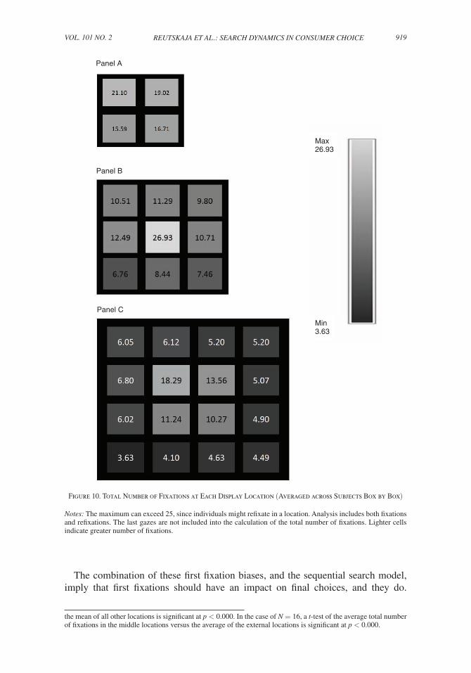
Figure 10 shows the same type of statistics for the total number of fixations at each location. If the first fixation effect completely wears off these numbers should be the same in all cells for each choice set size, but they are not. About a third of the fixations are in the upper-left for n = 4, and in the center item for n = 9 (compared


to random base rates of 25 percent and 11 percent respectively) and almost half of them are in the center four boxes for n = 16 (base rate 25 percent).5

5 In the case of n = 4, a t-test of the total number of fixations to the upper versus lower half of the display is significant at p < 0.000. In the case of n = 9, a t-test of the total number of fixations to the center location versus

Panel A

Panel B

Panel C

Max24.66

Min0.00

Figure 9. Total Number of First Fixations at Each Display Location (out of a Maximum of 25 and Averaged across Subjects Box by Box)

notes: Analysis includes first fixations only. Trials with only one fixation are included. Lighter cells indicate greater number of fixations.


The combination of these first fixation biases, and the sequential search model, imply that first fixations should have an impact on final choices, and they do.

the mean of all other locations is significant at p < 0.000. In the case of n = 16, a t-test of the average total number of fixations in the middle locations versus the average of the external locations is significant at p < 0.000.

Panel A

Panel B

Panel C

Max26.93

Min3.63

Figure 10. Total Number of Fixations at Each Display Location (Averaged across Subjects Box by Box)

notes: The maximum can exceed 25, since individuals might refixate in a location. Analysis includes both fixations and refixations. The last gazes are not included into the calculation of the total number of fixations. Lighter cells indicate greater number of fixations.


Figure 11 shows the choice frequencies. There is a small tendency to choose the upper items in n = 4, and much bigger biases in the other cases (60 percent above average for choosing the middle in n = 9, and 25 percent above average for the central four boxes in the case of n = 16).6

6 In the case of n = 4, a t-test of the total number of choices of items in the upper versus lower half of the display is significant at p < 0.051. In the case of n = 9, a t-test of the total number of choices of items displayed in the

Panel A

Panel B

Panel C

Max6.73

Min1.05

Figure 11. Total Number of Times the Item Displayed at Each Location was Chosen (Averaged across Subjects Box by Box)

note: Lighter cells indicate greater number of fixations.


Another way to measure the extent of the influence of display biases on choices is to ask what would happen if a retailer, for example, put the worst items (as judged by individual consumer ratings) in the locations at which they are likely to be seen first, or put the best items in those locations. How much would final choices vary in efficiency? Our design provides a ready answer to this question because items were randomly allocated to locations across trials. For each subject, we weight the likelihood that he will choose an item in a particular location by his total percentage of fixations in that location and compute the expected efficiency for the configura-tions of items he actually saw. We then create quartiles of “good displays” (in which the best items, as the subject judges them, are in the locations he tended to look at most often) and “bad displays” (in which the worst items are where he looked most often). The efficiencies in these quartiles are then averaged across subjects. Figure 12 shows the results. When the best items are in the visual “sweet spots” the efficiency is 91 percent—the subject is are almost sure to make the best choice. When the worst items are in the sweet spots efficiency is only 30 percent.

center location versus the mean of all other locations is significant at p < 0.000. In the case of n = 16, a t-test of the total number of choices made from items in the middle locations versus the mean of the external locations is significant at p < 0.000.

Q1 Q2 Q3 Q4

Weighted �xation efficiency

Cho

ice

effic

ienc

y

1

0.9

0.8

0.7

0.6

0.5

0.4

0.3

0.2

0.1

0

Figure 12. Choice Efficiency as a Function of Weighted Fixation Efficiency (by Quartile).

note: Error bars denote SEM.


The results in this section show that the choice process used by subjects when making decisions under time pressure could be potentially manipulated by inter-ested sellers. In field settings, this could be achieved by picking special locations in displays and supermarket aisles (Chandon et al. 2008), or by changing the packag-ing (e.g., by manipulating shape, size, and color) in a way that attracts first fixations through their impact in bottom-up and value-independent visual attentional mecha-nisms (Laurent Itti and Christof Koch 2001).

VII. Discussion

The goal of the current study was to set up an experimental version of the con-sumer’s supermarket choice problem, in which a choice among a large number of alternatives needs to be made under conditions of time pressure, in order to address the following three questions: (i) What are the computational processes deployed by consumers during the search and decision processes, and to what extent are they compatible with standard economic search models? (ii) How do the processes, and their performance, change with the number of options? (iii) Do the computational processes exhibit systematic biases that can be exploited by sellers to manipulate their choices? The results of the experiment provide insights about all of these questions.

First, we found that subjects are good at optimizing within the set of items that they get to see during the search process (the “seen set”); they choose items which are about 70 percent of the way from random to the maximum value in the set. But since the initial search process is approximately random with respect to value, it is not the case that items with higher value are more likely to be seen. We also find that subjects terminate the search process using a stochastic stopping rule that combines elements of optimal search and satisficing.

The experimental design allowed us to compare the ability of three alternative dynamic search models of how consumers might search and decide in these complex situations: a model of optimal dynamic search with zero search costs, a satisficing model, and a hybrid model in which subjects search for a random amount of time, which depends on the value of the encountered items, and then choose the best-seen item. The results provide strong support in favor of the hybrid model over the other two. Furthermore, a calibration of the hybrid model provides a good quantitative matched with time and choice quality properties of the observed data.

Second, we investigated how the search and choice process changed with the number of alternatives, which is a measure of the difficulty of the problem. We found that subjects respond to the additional pressure by shortening the duration of their fixations by about 60 ms and by searching for about 250 ms longer, thus increasing the number of options that are sampled before making a choice. However, the shift is modest compared to the increase in the number of items, and as a result it has only a small impact on the quality of the choices.

Third, we find that subjects exhibit a bias to look first and more often at items that are placed in certain regions of the display, which they also end up choosing more often. These effects are quantitatively large. For example, in the case of n = 9 an item in the center of the display was almost 60 percent more likely to be selected than similar items displayed in other locations. This feature of the process could be used to influence decisions which, depending on the motives of the individual


selecting the display, could be used to help consumers (e.g., by increasing the likeli-hood the high value items are seen) or to manipulate them (e.g., by using packaging and in-store displays to increase the probability that they purchase products that they would not have bought under more ideal conditions).

This is not the first paper using eye tracking–like technologies to study the process of information acquisition and decision processes in complex single-person choice environments. Payne, Bettman, and Johnson (1993) used Mouselab to study in mul-tiattribute choice environments and found that the pattern of search used by subjects depends on the complexity of the problem: with few numbers of options they search within items, whereas with large numbers of options they search within attributes. Gabaix et al. (2006) used Mouselab to test different theories of how subjects search in highly complex multiattribute choice spaces.

There are some important differences between our findings and these previous studies. First, we study search and decisions using displays in which options are described by pictures instead of list of attributes or matrices of payoffs (like look-ing at foods in a vending machine through glass, rather than looking at a restaurant menu with no pictures). The processes involved in these types of choice might be different, so our study expands the scope of understanding from numerical features into a domain of pictorial display which is widely used in actual choice. Second, we use eye-tracking for measuring fixations, which is arguably less intrusive than Mouselab, and more effortless for complex displays (Lohse and Johnson 1996). Third, we study decision in conditions of both option overload and time pressure. Fourth, in contrast to many previous studies on choice overload (Iyengar, Huberman, and Jiang 2004; Iyengar and Lepper 2000) where participants had an option to post-pone choice or not select anything at all and where participants faced unfamiliar items, we forced individuals to make a decision in every trial (which rules out the postponement of choice) and offered choice among highly familiar alternatives. Finally, we are able to propose a computational model of the search and decision processes that matches the data both quantitatively and qualitatively.

A comparison with previous research illustrates some differences between choice with and without time pressure. Krajbich, Armel, and Rangel (2008) have studied decision making using eye tracking from sets of binary options using a similar set of stimuli. They find that subjects often make repeated fixations to the same item before making a choice, and their fixations are almost 80 percent longer than the ones in this paper. One potential explanation for the difference with our results is that longer fixations are useful to improve the estimates of value. This is consistent with the findings of Armel, Beaumel, and Rangel (2008), and Armel and Rangel (2008). Similarly, repeated fixations might be useful to improve the comparison of values. If this is correct, the brain might compute noisier estimates of value (due to the shorter fixations) and might make more errors when comparing items, when making decisions under time pressure.

Economic readers might find the speed of search (with fixations around 350 ms) and choice (with decision times around 2,000 ms even in large choice sets) sur-prising. It is important to emphasize that these findings are in line with the previ-ous literature. For example (Milica Milosavljevic et al. 2009 found that people can actually make familiar binary choices in less than 400 ms while choosing the better item over 70 percent of the time.


One important question for future research is how well the computational model and biases identified here extend to other decision-making situations. We hypoth-esize that similar computational processes might be used by consumers in situations without time pressure in which they are overwhelmed by a large amount of informa-tion. A typical example would be the selection of an investment portfolio out of the long list of options offered by the typical investment company. Consumers might only end up considering a fraction of these options, and “marketing” factors such as location in display, color, font size, and style might affect which ones are actually considered and chosen.

An important lesson of our study is that the quality of choices is heavily influ-enced by the quality of fixations, but consumers might have limited control over their ability to sample the best items. A question for future research is therefore the extent to which consumers can train themselves to deploy better fixations, espe-cially in situations (such as the supermarket aisle) in which sellers might be trying to influence their decisions. Our hypothesis is that this might be possible, but that it might require costly training before the choice situation, and costly deployment of attentional control at the time decision making. For example, consumers might have to train themselves to look at random locations in displays and to ignore certain fea-tures of packaging such as color. Furthermore, deploying such rules might be hard in practice, since they require overruling powerful bottom-up attentional mechanisms (Itti and Koch 2001).

More generally, we believe that this paper illustrates the value for economists try-ing to understand the actual algorithms and computational processes that individu-als use to make different types of decisions. As described in the introduction, this approach has already generated important insights in behavioral game theory, but it has not been as widely applied in economics to individual decision-making pro-cess. The recent maturation of new technologies such as eye tracking and functional magnetic resonance imaging (fMRI) has made the development and testing of these types of models feasible and relatively low cost. These data should also be useful complements to theorizing about the details of the choice process (e.g., Caplin and Dean 2009; Dmitri Kuksov and J. Miguel Villas-Boas 2010; Pietro Ortoleva 2008).

REFERENCES

Armel, K. Carrie, and Antonio Rangel. 2008. “The Impact of Computation Time and Experience on Decision Values.” American Economic Review, 98(2): 163–68.

Armel, K. Carrie, Aurelie Beaumel, and Antonio Rangel. 2008. “Biasing Simple Choices by Manipu-lating Relative Visual Attention.” judgment and Decision making, 3(5): 396–403.

Bettman, James R., Mary Frances Luce, and John W. Payne. 1998. “Constructive Consumer Choice Processes.” journal of consumer Research, 25(3): 187–217.

Botti, Simona, and Sheena S. Iyengar. 2006. “The Dark Side of Choice: When Choice Impairs Social Welfare.” journal of Public Policy and Decision-making, 25(1): 24–38.

Brocas, Isabelle, Juan D. Carrillo, Stephanie W. Wang, and Colin F. Camerer. 2009. “Measuring Atten-tion and Strategic Behavior in Games with Private Information.” http://www-bcf.usc.edu/~brocas/Research/mousebetting.pdf.

Camerer, Colin F. 2003. “Learning.” In Behavioral Game theory: Experiments in strategic interac-tion, 265–335. Princeton, NJ: Princeton University Press.

Camerer, Colin F., and Eric J. Johnson. 2004. “Thinking about Attention in Games: Backward and Forward Induction.” In the Psychology of Economic Decisions, Volume 2: Reasons and choices, ed. Isabelle Brocas and Juan D. Carrillo, 111–29. New York: Oxford University Press.


Camerer, Colin F., Eric J. Johnson, Talia Rymon, and Sankar Sen. 1993. “Cognition and Framing in Sequential Bargaining for Gains and Losses.” In Frontiers of Game theory, ed. Ken Binmore, Alan Kirman, and Piero Tani, 27–47. Cambridge, MA: MIT Press.

Caplin, Andrew, and Mark Dean. 2009. “Choice Anomalies, Search and Revealed Preference.” Unpub-lished.

Caplin, Andrew, Mark Dean, and Daniel Martin. Forthcoming. “Search and Satisfying.” American Economic Review.

Chandon, Pierre, J. Wesley Hutchinson, Eric T. Bradlow, and Scott H. Young. 2008. “Measuring the Value of Point-of-Purchase Marketing with Commercial Eye-Tracking Data.” In Visual marketing: From Attention to Action, ed. Michel Wedel and Rik Pieters, 225–58. New York: Lawrence Erlbaum Associates.

Costa-Gomes, Miguel A., and Vincent P. Crawford. 2006. “Cognition and Behavior in Two-Person Guessing Games: An Experimental Study.” American Economic Review, 96(5): 1737–68.

Costa-Gomes, Miguel, Vincent P. Crawford, and Bruno Broseta. 2001. “Cognition and Behavior in Normal-Form Games: An Experimental Study.” Econometrica, 69(5): 1193–1235.

Gabaix, Xavier, David Laibson, Guillermo Moloche, and Stephen Weinberg. 2006. “Costly Informa-tion Acquisition: Experimental Analysis of a Boundedly Rational Model.” American Economic Review, 96(4): 1043–68.

Hare, Todd A., Colin F. Camerer, and Antonio Rangel. 2009. “Self-Control in Decision-Making Involves Modulation of the vmPFC Valuation System.” science, 324(5927): 646–48.

Hare, Todd A., Colin F. Camerer, Daniel T. Knoepfle, John P. O’Doherty, and Antonio Rangel. 2010. “Value Computations in Ventral Medial Prefrontal Cortex during Charitable Decision Making Incor-porate Input from Regions Involved in Social Cognition.” journal of neuroscience, 30(2): 583–90.

Hare, Todd A., John O’Doherty, Colin F. Camerer, Wolfram Schultz, and Antonio Rangel. 2008. “Dis-sociating the Role of the Orbitofrontal Cortex and the Striatum in the Computation of Goal Values and Prediction Errors.” journal of neuroscience, 28(22): 5623–30.

Harless, David W., and Colin F. Camerer. 1994. “The Predictive Utility of Generalized Expected Util-ity Theories.” Econometrica, 62(6): 1251–89.

Hey, John D., and Chris Orme. 1994. “Investigating Generalizations of Expected Utility Theory Using Experimental Data.” Econometrica, 62(6): 1291–1326.

Itti, Laurent, and Christof Koch. 2001. “Computational Modeling of Visual Attention.” nature Reviews neuroscience, 2(3): 194–203.

Iyengar, Sheena S., Gur Huberman, and Wei Jiang. 2004. “How Much Choice Is Too Much? Contri-butions to 401(K) Retirement Plans.” In Pension Design and structure: new lessons from Behav-ioral Finance, ed. Olivia S. Mitchell and Stephen P. Utkus, 83–95. New York: Oxford University Press.

Iyengar, Sheena S., and Mark R. Lepper. 2000. “When Choice is Demotivating: Can One Desire Too Much of a Good Thing?” journal of Personality and social Psychology, 79(6): 995–1006.

Johnson, Eric J. Colin Camerer, Sankar Sen, and Talia Rymon. 2002. “Detecting Failures of Back-ward Induction: Monitoring Information Search in Sequential Bargaining.” journal of Economic theory, 104(1): 16–47.

Jovanovic, Boyan. 1979. “Job Matching and the Theory of Turnover.” journal of Political Economy, 87(5): 972–90.

Knoepfle, Daniel T., Joseph Tao-yi Wang, and Colin F. Camerer. 2009. “Studying Learning in Games Using Eye-Tracking.” journal of the European Economic Association, 7(2–3): 388–98.

Krajbich, Ian, K. Carrie Armel, and Antonio Rangel. 2008. “The Role of Visual Attention in the Com-putation and Comparison of Economic Values.” Unpublished.

Kuksov, Dmitri, and J. Miguel Villas-Boas. 2010. “When More Alternatives Lead to Less Choice.” marketing science, 29(3): 507–24.

Lohse, Gerald L. 1997. “Consumer Eye Movement Patterns on Yellow Pages Advertising.” journal of Advertising, 26(1): 61–73.

Lohse, Gerald L., and Eric J. Johnson. 1996. “A Comparison of Two Process Tracing Methods for Choice Tasks.” organizational Behavior and human Decision Processes, 68(1): 28–43.

Luce, R. Duncan. 1959. individual choice Behavior: A theoretical Analysis. New York: John Wiley and Sons.

Maughan, Lizzie, Sergei Gutnikov, and Rob Stevens. 2007. “Like More, Look More. Look More, Like More: The Evidence from Eye-Tracking.” journal of Brand management, 14(4): 335–42.

Maule, A. John, and Anne C. Edland. 1997. “The Effects of Time Pressure on Human Judgment and Decision Making.” In Decision-making: cognitive models and Explanations, ed. Rob Ranyard, W. Ray Crozier, and Ola Svenson, 189–204. London: Routledge.


McCall, John J. 1970. “Economics of Information and Job Search.” Quarterly journal of Economics, 84(1): 113–26.

Milosavljevic, Milica, Alexander Huth, Vidhya Navalpakkam, Christof Koch, and Antonio Rangel. 2009. “Basic Psychometrics of Fast Value-Based Choice.” Unpublished.

Nagel, Rosemarie. 1995. “Unraveling in Guessing Games: An Experimental Study.” American Eco-nomic Review, 85(5): 1313–26.

Ortoleva, Pietro. 2008. “The Price of Flexibility: Towards a Theory of Thinking Aversion.” Unpub-lished.

Payne, John W., James R. Bettman, and Eric J. Johnson. 1993. the Adaptive Decision maker. New York: Cambridge University Press.

Pieters, Rik, and Michel Wedel. 2004. “Attention Capture and Transfer in Advertising: Brand, Picto-rial, and Text-Size Effects.” journal of marketing, 68(2): 36–50.

Pieters, Rik, Edward Rosbergen, and Michel Wedel. 1999. “Visual Attention to Repeated Print Adver-tising: A Test of Scanpath Theory.” journal of marketing Research, 36(4): 424–38.

Plassmann, Hilke, John O’Doherty, and Antonio Rangel. 2007. “Orbitofrontal Cortex Encodes Will-ingness to Pay in Everyday Economic Transactions.” journal of neuroscience, 27(37): 9984–88.

Rangel, Antonio. 2008. “The Computation and Comparison of Value in Goal-Oriented Choice.” In neuroeconomics: Decision making and the Brain, ed. Paul W. Glimcher, Colin F. Camerer, Ernst Fehr, and Russell A. Poldrack, 425–40. New York: Elsevier.

Reutskaja, Elena, and Robin M. Hogarth. 2009. “Satisfaction in Choice as a Function of the Number of Alternatives: When ‘Goods Satiate’.” Psychology and marketing, 26(3): 197–203.

Reutskaja, Elena, Axel Lindner, Rosemarie Nagel, Richard A. Anderson, and Colin F. Camerer. 2009. “The Boggled Mind: Choice Overload Reduces the Neural Signatures of Choice Set Value.” Unpub-lished.

Rubinstein, Ariel. 1988. “Similarity and Decision-Making under Risk (Is There a Utility Theory Reso-lution to the Allais Paradox?).” journal of Economic theory, 46(1): 145–53.

Russo, J. Edward. 2010. “Eye Fixations as a Process Tree.” In handbook of Process tracing meth-ods for Decision Research, ed. Michael Schulte-Mecklenbeck, Anton Kühberger, and Rob Ranyard, 43–64. New York: Psychology Press.

Russo, J. Edward, and France Leclerc. 1994. “An Eye-Fixation Analysis of Choice Processes for Con-sumer Nondurables.” journal of consumer Research, 21(2): 274–90.

Russo, J. Edward, and Larry D. Rosen. 1975. “An Eye-Fixation Analysis of Multi-Alternative Choice.” memory and cognition, 3(3): 267–76.

Van der Lans, Ralf. 2006. “Brand Search.” PhD diss. Tilburg University.Wang, Joseph Tao-yi, Michael Spezio, and Colin F. Camerer. 2010. “Pinocchio’s Pupil: Using Eyetrack-

ing and Pupil Dilation to Understand Truth Telling and Deception in Sender-Receiver Games.” American Economic Review, 100(3): 984–1007.

Wilcox, Nathaniel T. 2008. “Stochastic Models for Binary Discrete Choice under Risk: A Critical Primer and Econometric Comparison.” In Risk Aversion in Experiments. Research in Experimental Economics, Vol. 12, ed. James C. Cox and Glenn W. Harrison, 197–292. Greenwich, CT: JAI Press.

Willemsen, Martijn C., and Eric J. Johnson. 2009. “Observing Cognition: Visiting the Decision Fac-tory.” Unpublished.

search dynamics in consumer choice under time pressure: an eye

Documents