script solving economics and finance problems with matlab · script solving economics and finance...
TRANSCRIPT

Script
Solving Economics and Finance problems
with MATLAB
Peter H. Gruber
July 29, 2016

Useful shortcuts
+ Stop MATLAB: press ctrl-c
+ Restore the MATLAB screen:
HOME/Layout/Default
Desktop/Desktop Layout/Default (older MATLAB)
+ List of all symbols: see appendix D.1
+ Getting help: see section 2.4
+ Quick start: see section 2.3
About the author: Peter H. Gruber has been teaching MATLAB classes since 2005 at
the Universities of St. Gallen, Geneva and Lugano. He holds a PhD in Finance from
the Universita della Svizzera italiana in Lugano, an M.A. in Quantitative Finance
and Economics from St. Gallen University and a PhD in physics from the Vienna
University of Technology. He has worked for several years at CERN in the field of
neutrino physics and is currently a postdoctoral research associate at the Universita
della Svizzera Italiana in Lugano, Switzerland. His research interests include asset
pricing with a focus on volatility risk, high-performance numerical methods and big
data.
© 2007-2016 Peter H. Gruber, [email protected]
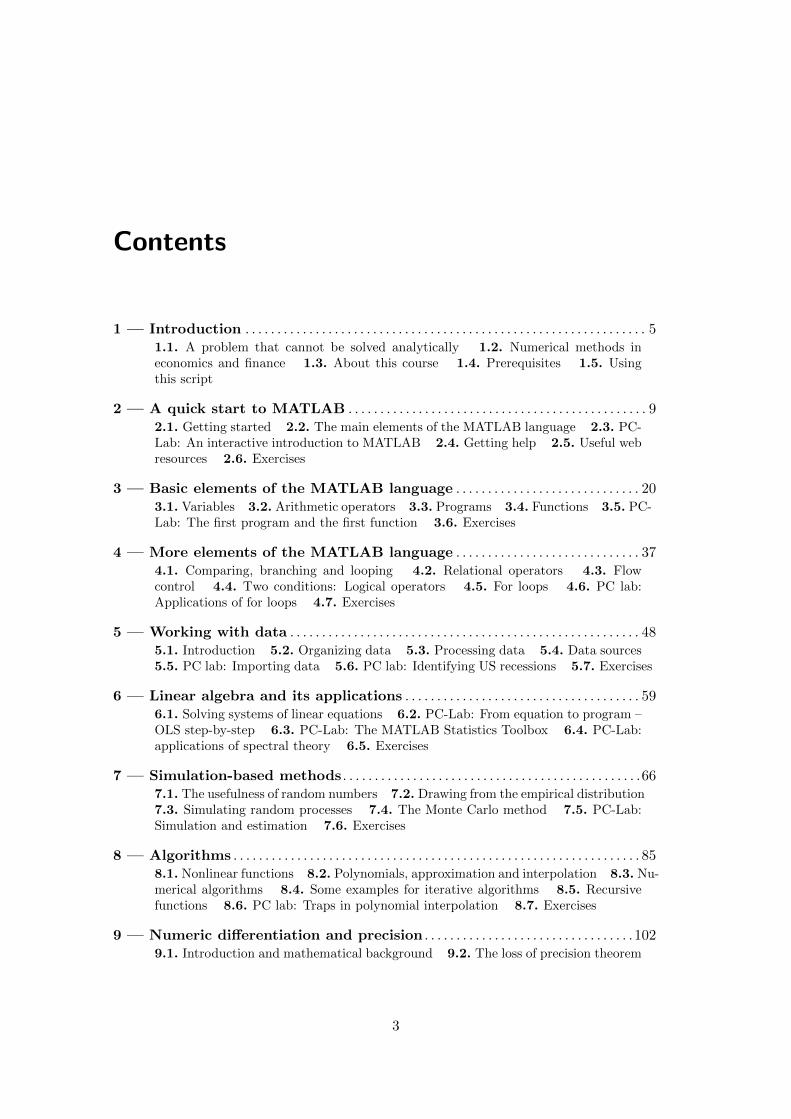
Contents
1 — Introduction . . . . . . . . . . . . . . . . . . . . . . . . . . . . . . . . . . . . . . . . . . . . . . . . . . . . . . . . . . . . . . . 51.1. A problem that cannot be solved analytically 1.2. Numerical methods ineconomics and finance 1.3. About this course 1.4. Prerequisites 1.5. Usingthis script
2 — A quick start to MATLAB . . . . . . . . . . . . . . . . . . . . . . . . . . . . . . . . . . . . . . . . . . . . . . . 92.1. Getting started 2.2. The main elements of the MATLAB language 2.3. PC-Lab: An interactive introduction to MATLAB 2.4. Getting help 2.5. Useful webresources 2.6. Exercises
3 — Basic elements of the MATLAB language . . . . . . . . . . . . . . . . . . . . . . . . . . . . . 203.1. Variables 3.2. Arithmetic operators 3.3. Programs 3.4. Functions 3.5. PC-Lab: The first program and the first function 3.6. Exercises
4 — More elements of the MATLAB language . . . . . . . . . . . . . . . . . . . . . . . . . . . . . 374.1. Comparing, branching and looping 4.2. Relational operators 4.3. Flowcontrol 4.4. Two conditions: Logical operators 4.5. For loops 4.6. PC lab:Applications of for loops 4.7. Exercises
5 — Working with data . . . . . . . . . . . . . . . . . . . . . . . . . . . . . . . . . . . . . . . . . . . . . . . . . . . . . . . 485.1. Introduction 5.2. Organizing data 5.3. Processing data 5.4. Data sources5.5. PC lab: Importing data 5.6. PC lab: Identifying US recessions 5.7. Exercises
6 — Linear algebra and its applications . . . . . . . . . . . . . . . . . . . . . . . . . . . . . . . . . . . . . 596.1. Solving systems of linear equations 6.2. PC-Lab: From equation to program –OLS step-by-step 6.3. PC-Lab: The MATLAB Statistics Toolbox 6.4. PC-Lab:applications of spectral theory 6.5. Exercises
7 — Simulation-based methods . . . . . . . . . . . . . . . . . . . . . . . . . . . . . . . . . . . . . . . . . . . . . . .667.1. The usefulness of random numbers 7.2. Drawing from the empirical distribution7.3. Simulating random processes 7.4. The Monte Carlo method 7.5. PC-Lab:Simulation and estimation 7.6. Exercises
8 — Algorithms . . . . . . . . . . . . . . . . . . . . . . . . . . . . . . . . . . . . . . . . . . . . . . . . . . . . . . . . . . . . . . . . 858.1. Nonlinear functions 8.2. Polynomials, approximation and interpolation 8.3. Nu-merical algorithms 8.4. Some examples for iterative algorithms 8.5. Recursivefunctions 8.6. PC lab: Traps in polynomial interpolation 8.7. Exercises
9 — Numeric differentiation and precision . . . . . . . . . . . . . . . . . . . . . . . . . . . . . . . . . 1029.1. Introduction and mathematical background 9.2. The loss of precision theorem
3

Contents
9.3. Tradeoff between numerical and analytical precision 9.4. Higher order algorithms9.5. Numeric differentiation of data 9.6. PC-Lab: Higher order differentiationalgortithms 9.7. Exercises
10 — Optimization . . . . . . . . . . . . . . . . . . . . . . . . . . . . . . . . . . . . . . . . . . . . . . . . . . . . . . . . . . . 11110.1. Metrics 10.2. Canonical formulation of the optimization problem 10.3. Con-vex optimization 10.4. Nonconvex optimization 10.5. Stochastic optimization10.6. Constrained optimization 10.7. PC lab: Fooling convex optimization 10.8. PClab: Stochastic optimization 10.9. Exercises
11 — Numeric integration and transform methods . . . . . . . . . . . . . . . . . . . . . . . 12711.1. The Riemann integral 11.2. Numeric integration 11.3. Numeric integrationof data 11.4. Transform methods 11.5. The FFT method for option pricing11.6. PC Lab: Comparing FFT and COS methods 11.7. Exercises
12 — How to write a successful program . . . . . . . . . . . . . . . . . . . . . . . . . . . . . . . . . . 14212.1. Introduction 12.2. Elements of good programming style 12.3. Finding codeand quoting it 12.4. Incomplete list of frequent MATLAB errors 12.5. Dos anddon’ts in MATLAB 12.6. PC lab: How good style prevents errors 12.7. Exercises
13 — Improving a program . . . . . . . . . . . . . . . . . . . . . . . . . . . . . . . . . . . . . . . . . . . . . . . . . . 15113.1. Debugging 13.2. Increasing a program’s efficiency 13.3. Dealing withcomplexity 13.4. Shortening a program 13.5. Exercises
14 — Parallel computing . . . . . . . . . . . . . . . . . . . . . . . . . . . . . . . . . . . . . . . . . . . . . . . . . . . . .16014.1. Introduction and concepts 14.2. Implementations of data parallel tasks inMATLAB 14.3. Exercises
15 — MATLAB and databases . . . . . . . . . . . . . . . . . . . . . . . . . . . . . . . . . . . . . . . . . . . . . . 16315.1. Introduction 15.2. Setting up a database system 15.3. Connecting MAT-LAB to the database
A — A recap of matrix algebra . . . . . . . . . . . . . . . . . . . . . . . . . . . . . . . . . . . . . . . . . . . . . 167A.1. Matrices, vectors and scalars A.2. Special matrices A.3. Matrix calculationrules A.4. Frequently used tricks with vectors A.5. Spectral theory A.6. Ap-plications of spectral theory
B — A recap of complex algebra. . . . . . . . . . . . . . . . . . . . . . . . . . . . . . . . . . . . . . . . . . . .180B.1. Exercises
C — An OLS refresher . . . . . . . . . . . . . . . . . . . . . . . . . . . . . . . . . . . . . . . . . . . . . . . . . . . . . . .182
D — Practical issues . . . . . . . . . . . . . . . . . . . . . . . . . . . . . . . . . . . . . . . . . . . . . . . . . . . . . . . . . 184D.1. MATLAB symbols D.2. MATLAB graphics D.3. MATLAB table outputD.4. From MATLAB to LATEX– creating a research workflow D.5. Practitioner’stips D.6. An introduction to the Symbolic Mathematics Toolbox
E — MATLAB @ UNI . . . . . . . . . . . . . . . . . . . . . . . . . . . . . . . . . . . . . . . . . . . . . . . . . . . . . . . 196E.1. Guide to the exercises E.2. Obtaining and installing MATLAB and its open-source alternatives
4

1. IntroductionI hear and I forgetI see and I rememberI do and I understandConfucius
1.1. A problem that cannot be solved analytically
Example 1. One of the most widely used distributions in economics is the standard normal
distribution. The probability density function (p.d.f.) is:
f(x) =1√2πe−
x2
2 (1.1)
What is the probability that one draw of a standard normal distributed random variable
is below, say, −1? The answer is given by the cumulative distribution function (c.d.f.):
Pr(X ≤ −1) = F (−1) =
∫ −1
−∞f(x)dx =
∫ −1
−∞
1√2πe−
x2
2 dx (1.2)
For the solution of this integral, we usually use a table or the computer. But how is the
value of the normal c.d.f. calculated? There is no simple representation. The only thing
we can do is to numerically integrate f(x): slice it into small strips and add up their area.
Fortunately, computers are very good at such boring, repetitive tasks (see section 11 for
the details). This short example illustrates that there are fairly simple problems that can
only be solved numerically.
1.2. Numerical methods in economics and finance
Numerical methods are widely used in economics and finance. They are at the core
of every econometric estimation. They are used for forecasting, asset pricing, scenario
generation, risk management and to optimize everything from truck routes to individual
spending behaviour, public policies and portfolios. As a rule of thumb, the more complex
or realistic a model becomes, the greater the chance that there is no analytical solution.
Literacy in numerical methods is nowadays often a job requirement in both economics and
finance.
5

1. Introduction
1.3. About this course
Philosophy
This script is not intended to be a cookbook, but rather a guide on how to invent new
recipes. The idea is to give the student a set of coloured stones from which she can make
her own mosaic. This means that equal emphasis is laid on understanding and using
the numerical methods presented here. This also implies that this script is organized by
methods rather than by topics. Techniques useful for, say, option pricing, can therefore
be found in the chapters on simulation, nonlinear functions and numerical integration.
The script is organized in three main parts: one for MATLAB, one for numerical meth-
ods and one for programming.
Part 1: Introduction to MATLAB
Section 2 is a jump-start into MATLAB and its language with an interactive introduction
that employs learning-by-doing starting on page 12. The basic elements of the MATLAB
language such as variables, operators, functions and programs are presented in section
3, while the more advanced concepts of flow control (if-then-else, loops), relational and
logical operators are covered in section 4.
Part 2: Numerical methods
Section 5 builds the foundation for every empirical work: how to organize and treat
data. Section 6 is about linear algebra and its applications to econometrics. Section 7
covers simulation based methods including Monte Carlo simulations. Section 8 discusses
nonlinear functions and a few standard problems in numerical mathematics: root finding,
fixed points and inverse functions. Section 9 is devoted to numerical differentiation and
the associated precision problems. Section 10 covers the important topic of optimization.
Sections 11 discusses numerical integration, including a presentation of the FFT-Algorithm
(Fast Fourier Transformation).
Part 3: The art of programming
Sections 12 and 13 are two of the most important sections on the road towards a successful
numeric project. They develop a framework for the successful management of a program-
ming project and give clear guidelines on how to avoid and detect errors. Sections 14 and
15 contain useful additions: an introduction to parallel computing and an introduction to
databases.
6

1. Introduction
The appendices feature reference and review material, and practitioner’s tips.
1.4. Prerequisites
Student’s knowlegde. No programming knowledge is needed for this script, which aims
at being mostly self-contained. Students profit from bachelor level knowledge in mathe-
matics (matrix calculus, functional analysis, complex analysis), finance (definition of basic
assets and their payoffs), econometrics (OLS) and probability (moment generating func-
tions).
Software. MATLAB comes with literally hundreds of toolboxes, each of which has to be
paid for separately. Therefore this course is limited to using the statistics and econometrics
toolboxes, which come with the student edition of MATLAB. Several chapters profit from
additional free toolboxes, see page 190 on how to install these toolboxes. All code has
been tested with MATLAB 2012b, but should run with any version after 2005b.
1.5. Using this script
The main idea of this course is to combine systematic knowledge with learning by doing.
It is best to keep an open MATLAB session while studying.
Theory stands at the beginning of every chapter: to explore how and why certain methods
work, as well as their limits and precision.
Examples denoted |MATLAB examples illustrate the new concepts. They should be
entered into the MATLAB command window while reading the text.
PC labs give the reader a guided tour through a new concept. They are an integral part
of this course – some details are only shown in the PC labs. Usage is simple: enter
the commands in the command window, watch the results and read the explanation.
Exercises Programming is a matter of experience. The PC labs can only be a starting
point, thus the reader is more than invited to try at least a few exercises per chapter.
Some of the exercises are used as problem sets for grading, therefore no solutions
will be published. Appendix E.1 contains my guidelines for solutions.
Notation and fonts
Capital letters (A) denote matrices, small caps (a) vectors and scalars. Bold small caps (x)
always denote vectors, Greek letters (α, . . . ) always scalars. Vectors are usually column
vectors. They are often written using the transpose to save space: x = (x, y)′ =(
x
y
).
7

1. Introduction
MATLAB commands are printed in the font teletype (e.g. plot). To avoid duplication,
they are usually not explained in all detail. This is much better done by MATLAB’s help
function (e.g. help plot) or the Mathworks website. Menu items are printed in sans serif,
with sub-menus separated by a forward slash (e.g. Help/Full Product Family Help).
NOTE: important remarks are denoted with this symbol.
TIP: practitioner’s tips (not mandatory, but useful) are marked with this symbol.
* material or exercises which are a bit more challenging are marked with an asterisk.
M material very specific to the MATLAB language is marked with a superscript M .
Students focusing on numerical methods in general may wish to skip these sections.
Resources
This script comes with a set of sample programs, data sets and a set of slides. Solutions
to the exercises will not be provided.
Acknowledgements
This text has been vastly improved thanks to input from my students at the University
of St. Gallen. Further suggestions and corrections to [email protected] are always
welcome. I am grateful to Roman Meyer, Daniel Kohler, Nick Galli and Marco Hurner
who gave valuable comments to the first versions of this script. I take the sole responsibility
for all remaining errors.
8

2. A quick start to MATLAB
References: Getting started with MATLAB, sections 1, 2 and 6-1 to 6-13; Moler; Hansel-
man and Littlefield
2.1. Getting started
TIP: If your screen does not look like Fig. 2.1, click Desktop/Desktop Layout/Default.
(1) Command Window. The command window has two uses. First, MATLAB com-
mands can be directly entered here (“interactive mode”). This can be used for pocket
calculator-like operations. All output – be it from a direct command or from a program –
is also displayed in the command window.
Direct input in the command window is a fast way to test new ideas. Once the results
are satisfactory, the command history (3) can be used to assemble a program (see Sec. 3.5).
4
32
1
5 6
7
8
Figure 2.1.: MATLAB screen (version 2013a).(1) Command window, (2) MATLAB Tool-strip, (3) Current Directory Bar, (4) Current Directory Window, (5) ProgramEditor, (6) Workspace, (7) Command History, (8) Quick Access Toolbar.
9

2. A quick start to MATLAB
(2) MATLAB Toolstrip. The toolstrip is organized by topic. Its contents depend on the
context. Some important commands can only be found here, e.g. for the editor (indent,
outdent, (un)comment) or for graphics.
(3) Current Directory Bar Very important: By default, everything will be loaded or
saved from/to this directory.
(4) Current Directory Window The contents of the current directory are shown in this
window. If you double-click a program, it will be opened in the program editor (4). If you
double-click on a data file, it will be loaded/imported.
(5) Program Editor. Here you can write and edit your programs.
(6) Workspace Note that at the lower end of the current directory window, there is
a tab where you can switch between the current directory view and the workspace (2).
The workspace is a view into the “memory” of MATLAB. Here, you can see all current
variables and their values. When going through the interactive introduction to MATLAB
in section 2.3, keep an eye on the workspace and observe how the variables evolve.
(7) Command History. A list of all commands that have been entered, in reverse chrono-
logical order. The command history can be used to create a program from trials in the
interactive mode (see section 3.5).
(8) Quick Access toolbar. A list of symbols that allow quick access to often-used com-
mands in every context. See the appendix on how to modify the toolbar.
Getting started with MATLAB alternatives. Octave is an open source (=free) program
with a command set almost identical to MATLAB. You can think of the Octave user
interface as having only a command window. Octave uses special commands for all other
elements. The workspace is replaced by the who command, the current directory window
by the commands ls, pwd and cd, the command history by history. Octave has no
program editor, you have to use the external editor of your choice. See Appendix E.1 for
how to install Octave and other MATLAB alternatives.
TIP: For a trial of Octave without installing anything on your computer, go to
http://lavica.fesb.hr/octave/octave-on-line_en.php or
http://www.compileonline.com/execute_matlab_online.php
10

2. A quick start to MATLAB
2.2. The main elements of the MATLAB language
Variables. Variables are created implicitly, i.e. by assigning a value to them. The com-
mand a=1 performs two things: (1) a variable called a is created, and (2) the value 1
is assigned to it. Variables can be of different types: scalar, vector, matrix (like their
mathematical counterparts) and string (for text). Note that the names of variables are
case sensitive (so A is not the same as a). Variables should be named with self-explaining
names, see section 3.1.
Arithmetic operators. An operator is best explained with an example: +,−, ∗, / are all
arithmetic operators. The hat ^ stands for the power operator, e.g. 52 is written as 5^2.
(Remember that n√x = x1/n). The order in which operators are executed is called operator
precedence. Example: 2+3*5. The multiplication is executed before the sum. For details,
see section 3.2 and Tab. 3.3.
Relational operators. So-called relational operators compare two variables and give the
results true or false. Among these are: equal (==), not equal (~=), less (<), less or equal
(<=), greater (>), greater or equal (>=). Relations can only be true or false. MATLAB
assigns numerical values to these two: true=1 and false=0. Example: 2<3 is true (or 1),
4.4==4.5 is false (or 0). For details, see section 4.2.
Logical operators. Most noteworthy are “and”(&), “or” (|) and not (~). They are used
to combine two conditions. Example: (2<3) | (4.4==4.5) is true, because one of the
two comparisons is true. For details, see section 4.4.
Functions. A MATLAB function works like a standard mathematical function: it takes
one or more arguments and produces one or several results. Widely used built-in func-
tions are log(), exp(), abs(), sqrt(). MATLAB extends the concept of a function
to vectors. Example: given a vector x = (x1, x2, x3), MATLAB computes log(x) =
(log(x1), log(x2), log(x3)) .
Apart from these built-in functions, users have the flexibility to write self-defined func-
tions. Note that these work only as well as they have been programmed. User-defined
functions are only vector compatible, if the user has explicitly provided for this. Generally,
a user-defined function must be saved in a separate m-file. See section 3.4.
Flow control. Many computational algorithms require repeating certain steps, often as
a function of previous results. In MATLAB, a block of code can be executed several times
11

2. A quick start to MATLAB
(using for, while) or subject to a condition (using if-else, switch-case). See section
4.3.
Comments. MATLAB ignores all text after a percent sign (%) until the end of the line.
Start a line with % for long comments or add a short remark after a command in the same
line. Comments are an important element of programming style, see Section 12.1.
Data input and output. Calculations would make no sense if there is no output of the
results. By default, MATLAB prints the result of every calculation in the command
window. To suppress the output of intermediate results, end the respective line with a
semicolon (;).
It is not customary to let the user interactively input data. Small amounts of data such
as parameter choices are often specified in the first block of a program. Larger amounts
of data are usually stored in a separate data file. MATLAB can directly access many
database systems and read and write various file formats, including CSV and MS Excel.
See Chapter 5.
Graphics are a special form of data output. MATLAB supports a wide range of plot
types, see Appendix D.2.
Toolboxes are libraries of useful functions for a certain field. The Mathworks sell some
90 different toolboxes, of which about a dozen are relevant for economics and finance.
Programs that rely on a toolbox will only run on machines where this toolbox is installed;
this is impractical if several people work on a project. There is an increasing number of
open source toolboxes, see the web links in section 2.5.
2.3. PC-Lab: An interactive introduction to MATLAB
MATLAB is best explained by using it. Just enter the commands in the command window
(see Fig. 2.1) and press return. Observe the output and possible changes in the workspace.
A short explanation is given for every command; detailed explanations follow in the two
subsequent chapters.
Before getting started
TIP: MATLAB’s diary command makes it possible to save the results of this interactive
introduction. First, verify that the current directory (see Fig. 2.1) is set suitably.
TIP: If you have not yet done so, bring the workspace to the front and keep an eye on the
MATLAB workspace while working through this introduction.
12

2. A quick start to MATLAB
diary(’intro.txt’) Set the diary file name and start recording.
% My first MATLAB session Start the line with a ’%’ to make a comment. They will
show up in the diary and help you remember.
Matlab as a pocket calculator
1+1
2+3*5 MATLAB observes the correct operator precedence.
Variables
a Error message, because the variable a has not yet been created.
a=2 This does two things: (1) create a variable a and (2) assign the value 2
to this variable. Watch the workspace (see Fig. 2.1).
a Recall the value of the variable.
b=3.5 Define a variable b with value 3.5 (its a dot and not a comma!)
b=3,5 The comma (,) means next command ...
b=3, c=5 e.g. to write two commands in one line (rarely used).
A You receive an error message; there is no variable A (only small a).
Commands and the names of variables and files are case sensitive.
Arithmetic operators
a+b Arithmetic operators are + - / * and ^ for “power”.
a-b Negative numbers are simply entered with a minus in front.
d=a+b Assign the result of a calculation to a new variable.
a+b*c Operator precedence
(a+b)*c Round brackets have the highest precedence. Note: every shape of
brackets has its own meaning, see Appendix D.1.
((a+b)*c+a)/b Several levels of brackets are all defined with the round bracket ().
a^b Power.
a^b+c This may produce an undesired result . . .
a^(b+c) If you want to enter ab+c, you have to use a bracket.
a^2 Squared
sqrt(a) Square root. But is there also a command for the third root of a?
a^(1/3) There is none. We need to use our mathematics knowledge: 3√x = x1/3.
a^0.33 Compare the resuts. TIP: never perform computations for the computer!
13

2. A quick start to MATLAB
Some floating point formatting
format long Display output with full 15 digit precision.
[2xcursor up] Cursor up gives the last input. Cursor up twice should give you a^0.33.
[0.01 1250 2.25] Typical financial data.
format bank Useful.
format short NOTE: format only changes the display – not the result of the calculation.
Functions
log(a) Natural logarithm (some people write ln() for it) ...
log10(a) ... as opposed to the logarithm with basis 10.
exp(a) Exponential.
abs(-3) Absolute value.
rand Function without arguments. Try several times. Use [cursor-up]
help rand Does rand really have no arguments? Use the help function to find out.
Errors and NaN (not a number)
log(0) A pocket calculator would give an error, here.
e=0/0 Another error. NaN stands for not a number.
1+e Calculations with NaN are possible, but most of the time not very useful.
Vectors
xRow=[1, 3, 7] This creates a row vector: commas separate the columns of a vector.
yRow=[2 5 1] The commas are not needed: use spaces as shortcut.
aCol=[3; -1; 1] The semicolon means “new line” (We mostly use column vectors.)
bCol=[3 -1 1].’ Transposing a row vector is a fast way to enter a column vector.
CAREFUL: The transpose is a.’ while a’ means complex conjugate.
xRow*yRow Error message, because two row vectors cannot be multiplied.
xRow*aCol Vector product: row times column vector.
aCol*xRow The vector product is usually not commutative.
aCol(1) Obtain a specific element of a vector.
aCol(1) = 9 Change a specific elements of a vector.
xRow(2) = 0 Set one element of zero. This is not the same as ...
xRow(2) = [] deleting one element of the vector. Compare the result to the line above.
xRow(end) Obtain the last element of x.
xRow(end+1) = 8 Add an entry at the end of the vector.
xRow=[xRow 7] Grow the vector xRow. Can be done several times using [cursor up]
14

2. A quick start to MATLAB
Matrices
zMx=[1 2 3; 4 5 6; 7 8 9] creates a 3× 3 matrix
zMx(1,2) Before hitting return, predict the result. Remember: row, column
zMx*aCol Matrix times vector.
zMx*xRow If the dimensions do not match you get an error message.
eye(3) Identity matrix: Multiply any vector or matrix with it ...
eye(3)*aCol ... and it remains the same. Try this for xRow, zMx.
Semicolon and colon
a+b; ASuppress output. This seems to make no sense here, but ...
d=a+b; ... virtually all lines in MATLAB end with a semicolon.
1:5 The colon operator produces a vector in steps of 1.
1.2:5.5 Remaining fractions in the interval are ignored.
xRow(1:2) Main use of the colon operator: to access a range of elements.
xRow([1 2]) These two things are the same.
xRow([3 1 2]) We can even change the order of elements.
xRow(1:end-1) Get all but the last elements – an often used application.
More on vectors and matrices
uMx=[aCol bCol] Create a matrix by concatenating column vectors.
vMx=[zMx aCol] We can even concatenate matrices and vectors.
load stocks.mat Load some sample data: returns of 10 different stocks.
size(stocks) Obtain the dimensions of our data set: number of rows, columns.
stocks(1:end,1) First column only, i.e. the returns for stock number 1.
stocks(:,1) Shortcut for first column.
stocks(2,:) Second row only, i.e. the returns of all stocks on day 2.
stocks(:,[2 4 7])Subset of stocks number 2, 4 and 7.
mean(stocks) Average return per stock: make use of matrix-compatible function.
std(stocks) Daily standard deviation per stock.
True or false?
1<2 This is of cause true. In MATLAB: true=1 and ...
0==1 false=0. Note the double equality sign for comparisons.
aCol<bCol Vectors and matrices are being compared element-by-element.
15

2. A quick start to MATLAB
Plots
plot(stocks) All 10 stock returns in one.
plot(stocks(:,1)) Just the first stock.
plot(stocks(:,1),stocks(:,2),’o’) Scatter plot. Stocks one and two are correlated.
plot(stocks.’) Undesired result: MATLAB expects data series in rows.
plot(cumsum(stocks)) Cumulative returns for all stocks.
hist(stocks(:,1),10) The command hist(x,n) produces a histogram with n bins.
hist(stocks) Ten histograms in 1 plot.
diary off Turn off the diary. It is in intro.txt in the current directory.
TIP: Now is a good time to have a look at Appendix D.1, which lists all MATLAB symbols.
2.4. Getting help
• In the command window, use help <command>
• For more general help, type lookfor <concept>
• Use the menu Help/MATLAB Help
• You can also get help by right-clicking any command and choosing Help on Selection.
• Demo programs: use demo to get a list. Interesting demos include travel, a travel-
ling salesman problem.
• All of the excellent MATLAB user guides are available on www.mathworks.com
2.5. Useful web resources
• Programs
– www.mathworks.com
– freemat.sourceforge.net
A MATLAB compatible open source program with editor and graphics support.
– www.gnu.org/software/octave/
Homepage of Octave, the free program that is compatible to MATLAB.
– lavica.fesb.hr/octave/octave-on-line_en.php
Online version of Octave.
• Code
– www.matlabcentral.com
MATLAB file exchange, newsgroups and blogs.
– www.wilmott.com, www.nuclearphynance.com, mathfinance.com, mathfinance.cn
Online quant finance communities. A lot of code is also useful for economists.
16

2. A quick start to MATLAB
– www.statsci.org/matlab.html
Statistical toolboxes for MATLAB.
– www.spatial-econometrics.com
A comprehensive and well-documented econometrics toolbox.
– www.kevinsheppard.com
Homepage of the MFE financial econometrics toolbox.
– home.tiscalinet.ch/paulsoderlind, www.mathworks.com/moler
Homepages of distinguished researchers with useful resources.
• Some further reading:
– history.siam.org
The history of numerical analysis and scientific computing.
• Data → page 48.
2.6. Exercises
Exercise 2.1. Calculate
(a) 1/10−6 (b) 4√
22 (c) 43+2 (d) 4+712−2 (e) (12− 5)4/3 (f) 22
33(g) ln(2+3
4−1)
Exercise 2.2. Working with functions
(a) Calculate ln ex and elnx for x = 2;x = 10 and x = 20. Are the results equal to x, as
expected? Hint: use format long
(b) Produce a neat table (i.e. a matrix) with the values of the sin and cos for 0, π/2,
. . . 2π. Produce a vector of arguments in the first step, then the matrix with results.
(c) Produce the value of e (the Euler number).
Exercise 2.3. (Use of the colon operator)
(a) Produce a row vector x with the integers from 1 to 10.
(b) Produce a 5 × 5 matrix with the integers from 1 to 25. Hint: combine the matrix
from five row vectors.
(c) Produce a multiplication table by calculating the outer product of x with itself
(i.e. multiply x with x in such a way, that you get a matrix as result).
Exercise 2.4. Start with load(’count.dat’). This data contains hourly counts of num-
ber of vehicles that pass at three different observation points.
17

2. A quick start to MATLAB
(a) Produce a matrix c1, which is the top left 12× 2 submatrix of count.
(b) Produce a vector c2, which is the 2nd row vector of count.
(c) Produce a vector c3, which is the 3rd column vector of count.
(d) Produce a matrix c4, which consists of the 1st and 3rd columns of count.
(e) Multiply count with a suitable vector such that the result contains the sum of the
number of cars over the whole day for each of the three observation points.
(f) Produce a matrix c5, which contains the data for all three observation points for the
even hours of the day (i.e. 2 a.m., 4 a.m. until midnight).
(g)∗ It turns out that the counts for observation point 1 and 2 have been swapped for
the evening hours, starting at 18:00 hrs. Create a new matrix c6 that corrects this
mistake.
18

2. A quick start to MATLAB
Exercise 2.5. Start with load stocks.mat, see the interactive intro to MATLAB.
(a) Calculate the correlation matrix of the first, the third and the seventh stock.
(b) Create a matrix s1, in which you eliminate day number 27 from the sample.
(c) Create a vector s2 that contains the weekly returns from the first week (5 trading
days).
(d) Create a matrix s3 that contains the five weekly returns from the first five trading
weeks by concatenating five vectors of weekly returns.
Exercise 2.6. Produce a vector x that contains 100 standard-normal random numbers.
(a) Calculate the mean of the first twenty elements, then for the second twenty elements
and so on.
(b) Repeat (a) for the variance. Use the help function to find the necessary command.
(c) Create two vectors y,z that contains the first/last 50 observations. Calculate the
covariance of y with y, y with z and z with z.
(d)∗ Repeat (a) to (c), but do not use MATLAB’s built-in commands for the mean, the
variance and the covariance. Use vector multiplication instead.
Exercise 2.7. Start with A=magic(5). This creates a 5× 5 magic square.
(a) Produce a matrix B, which is the top left 3× 3 submatrix.
(b) Produce a 5× 2 matrix C, which consists of the 1st and 4th column vectors of A.
(c) Explain briefly (in a comment) what the command magic does. (Use help).
(d)∗ Produce a vector w that contains the diagonal elements (aii) of A.
19

3. Basic elements of the MATLAB language
References: Hanselman and Littlefield; Mathews and Fink, section 6; Brandimarte ap-
pendix A; Getting started with MATLAB, section 2; Opfer
3.1. Variables
3.1.1. Facts about variables
Variables are the building block of every computing language. They work much like in
“paper mathematics”. To square a specific number, e.g. three, we write 32. To express
that any given number x be squared, we write x2.
In MATLAB, every variable has a value. Think more of a “variable” or a “placeholder”
than of an “unknown”. Variables live until cleared by the command clear or MATLAB
is shut down.
Implicit declaration When you enter a=1, two things happen: First, a variable called a is
created and second, the value of 1 is assigned to a. Some programming languages require
that variables be defined (“declared”) before use; this is not the case in MATLAB.
TIP: Some useful commands: who, whos, clear, disp
Naming The big difference to “paper mathematics” is that the name of a variable can
be as long as 63 characters in MATLAB. All letters of the alphabet and numbers are
allowed, however no spaces, umlauts or accented characters. Some names should not be
used: i and j (reserved for complex numbers) and the names of MATLAB commands.
Long names make variables self-explaining (e.g. output instead of Y).
Names in MATLAB are case sensitive, so Output would not be the same as output.
TIP: It is a good idea to adopt a personal naming convention right from the start. Two
popular conventions are “lowercase underscore” (e.g. is good student) and “cap-
italized words” (e.g. IsGoodStudent). See section 12.2.2.
20

3. Basic elements of the MATLAB language
Decimal 0 1 2 3 4 5 6 7
Binary 000 001 010 011 100 101 110 111
Table 3.1.: All 3-bit binary numbers.
bit component range
1 sign +/-2-12 exponent w/ sign [2−1022 21024]
13-64 significand (mantissa) [2−52 0]
Table 3.2.: The IEEE Standard 754-1985 for double precision floating point numbers.
3.1.2. Floating point representation and numerical precision
Computers use bits to store and manipulate information. A bit has only two states: on
or off. They correspond to the digits zero and one. Using several (e.g. 16) bits, one can
store information in the form of binary numbers. Example: With three bits, one can store
the numbers from 0 to 7, see Tab. 3.1.
The binary system is only defined for positive integers. To be able to use real numbers,
possibly very large ones, computers use the floating point representation:
x = ±m× 10±k (3.1)
x = ± m e± k (3.2)
where m is called significand (or mantissa) and k is called exponent. The second line
shows how MATLAB outputs floating point numbers, e.g. 1.23e-2 for 1.23× 10⁻².
Example: floating point representation
1.23e-2 Enter a small number in floating point notation.
7.56e4 A large number.
format shorte Output in floating point notation.
1.1+2.2 Note: e00 means ×100, i.e. “times 1”.
Today’s standard computer arithmetics, which is also used by MATLAB, employs 64 bits
to store one floating-point number (see Tab. 3.2). It is defined in the IEEE Standard 754-
19851. The maximal and minimal numbers that can be expressed precisely in this standard
are determined by the significand. They are 252 = 4.5× 10¹⁵ and 2−52 = 2.2× 10⁻¹⁶. The
latter number is sometimes called eps from the Greek letter epsilon (ε) that usually denotes
infinitesimal quantities. MATLAB provides a function called eps that returns 2.2204e-16.
1A simplified version of the floating point standard is presented at tinyurl.com/IEEE754.
21

3. Basic elements of the MATLAB language
The maximal and minimal exponents are: 2−1022 and 21024, i.e. 2.225×10−308 and 1.798×10308. They can be reproduced using the functions realmin and realmax. The smallest
number that MATLAB can handle at all is eps*realmin=4.94E-324. Any number smaller
than that is seen as zero.
Example: limited precision of floating point numbers
format long Display all 15 digits.
4.9+3.3 A rather simple expression. Guess the result before hitting return.
a=1+1E-16; Add two numbers; one comparatively smaller than the other one.
a-1 We would expect 1E-16, however, MATLAB returns 0.
NOTE: For more on precision, see sections 9.2 and 13.
3.1.3. Working with variables
Types. The type of a variable describes (a) the type of information that it stores, e.g. num-
bers or text and (b) the dimension, e.g. scalar, vector or matrix. In MATLAB, every
variable has a type, which is assigned automatically at creation. Some operations are only
possible or sensible for certain types. As a type cannot be seen from a variable’s name,
it is your task to ensure the correct type of each variable. For this reason it is also a bad
idea to change the type of a variable during the course of a program (even though it is
possible).
Example: Types and type mismatchesa=[1 2] Create a vector with 2 elementsb=[1 2 3] Create a vector with 3 elementsa+b MATLAB error: Matrix dimensions must agree.
t1=’one’ Create a text variablet1+b Strange results when mixing types’one’ + ’two’ Even stranger resultswhos Produce a list of variables with type and dimension
Matrices
Matrices are the native variable type of MATLAB (in fact, the name stands for “matrix
laboratory”). MATLAB uses the standard notation for matrices, in which the dimension
is quoted as rows×columns. Similarly, an element of a matrix is accessed as (RowNumber,
ColumnNumber).
Matrix dimensions and element position: row × column
22

3. Basic elements of the MATLAB language
1,1 1,2 1,3
2,1 2,2 2,3
3,1 3,2 3,3
1 4 7
2 5 8
3 6 9
(a) (RowIndex, ColumIndex) (b) (SingleIndex);
Figure 3.1.: Two alternative ways to access the elements of a matrix: by row index andcolumn index or by single index.
To create matrices, use the following commands:
• Create a matrix from data: Zmatrix = [1 2 3; 4 5 6; 7 8 9];
• Create from column vectors: Zmatrix = [aCol bCol cCol];
• Create from row vectors: Zmatrix = [xRow; yRow; zRow];
• Create from same vector: Zmatrix = repmat(vector, nRows, mCols)
• Standard matrices: eye(n) (identity), zeros(m,n), ones(m,n)
• Matrices of random numbers: rand(m,n), randn(m,n), randi(imax, m,n)
To manipulate matrices, use the following commands (see also Fig. 3.1):
• Access an entry by row and column: Z(RowIndex, ColumnIndex)
• Access a whole row: Z(RowIndex,:)
• Access a whole column: Z(:,ColumnIndex)
• Delete a row: Z(RowIndex,:)=[]
• Grow a matrix by adding a column vector: Z=[Z aCol]
• Get the dimensions of a matrix: size(Z)
• *Access an entry by single index (rarely used): Z(SingleIndex)
The commands ind2sub() and sub2ind() convert to and from single notation.
TIP: Useful commands: sum(X), min(X), max(X), mean(X), sort(X)
Example: Working with matricesload stocks A sample data set of simulated stock returnsstocks(:,1) Returns of first stockmyPF=[1 4 7] My portfolio contains stocks number 1,4 and 7stocks(:,myPF) Returns of stocks in my portfoliomyWt=[0.2 0.7 0.1].’ My portfolio weightsstocks(:,myPF)*myWt Returns of my portfolio
23

3. Basic elements of the MATLAB language
Example: System of linear equations Ax = bA=[-1 3; -1 1]; Parameter matrixb=[-6 2].’; Result vectorrank(A)==min(size(A)) Does the matrix A have full rank?x=inv(A)*b Solution.
Example: Covariance of two random numbersN=1000; Good programming style: define parameter firstX = randn(N,2); Produce matrix containing two random numbersX.’*X/(N-1) Calculate the covariance matrix (supposing zero mean)cov(X) Zero mean assumption was wrong.Y=X-repmat(mean(X),N,1) Subtract mean from each row.Y.’*Y/(N-1); Correct covariance matrix
Vectors
MATLAB has in fact no special provisions for vectors. A row vector is seen as a 1 × Nmatrix, and a column vector as a M × 1 matrix. This matrix view bears the advantage
that we can use all the matrix commands for vectors, as well.
Commands for creating vectors:
• Create row vector: xRow=[1, 2, 3] or xRow=[1 2 3]
• Create column vector: aCol=[5; 6; 7] or aCol=[5 6 7].’
NOTE: The latter version is widely used.
• Create row vector with with M elements: linspace(start, end, M)
Commands for manipulating vectors:
• Concatenate row vectors with space: [xRow yRow]
• Concatenate column vectors with semicolon: [aCol; bCol]
• Access/delete the n-th element: x(n) and x(n)=[]
• Access last element: x(end)
• Get the length of a vector: length(x)
• Grow an existing column vector: aCol=[aCol; 7] or aCol(end+1)=7
• Convert any matrix or vector into a column vector: y=x(:)
• Vector plus scalar: in standard mathematics, the operation x + α is not defined. In
MATLAB, the value of α is added to every element of the vector x.
Vector products are widely used in MATLAB to calculate sums.
Sum of sqaures x′x =∑n
i=1 x2i SSE= u.’*u
Weighted sums x′y =∑n
i=1 xiyi E = probability.’ * outcome
24

3. Basic elements of the MATLAB language
Figure 3.2.: A three-dimensional array can be seen as a time series of matrices.
Example: Reproduce the famous Fibonacci series using a growing vector.
fib = [1 1] Start with the first two numbers as defined
fib(end+1)=fib(end-1)+fib(end) New element is sum of last 2 elements.
[cursor up] [return] Repeat as often as you like.
MThe colon operator MATLAB has a special operator for creating vectors: the colon
operator. There are two syntaxes to use it.
Syntax of the colon operator1:5 min : max produces a vector in steps of 1.1:0.5:5 min : ∆ : max steps of ∆ = 0.5.5:-1:0 Note: ∆ can also be negative.1.2:4.5 If the range max−min is not integer, the last fraction is discarded.
Datasets
Datasets are convenient way to work with cross-sectional data matrices, where each column
corresponds to one variable. A good example is provided by MATLAB’s cereal data:
Datasetsload cereal Data set containing cereal nutrition datacereal = dataset(Calories,Protein,Fat,Sodium,...
Fiber,Carbo,Sugars,’ObsNames’,Name)
cereal Output the dataset in nice tablecereal.Fat Access one column on the dataset
*Arrays
Example 2. Imagine you are performing a portfolio analysis with historic data. For every
quarter in the last year, you have a correlation matrix of all assets, i.e. 4 correlation
matrices as depicted in Fig. 3.2. Is there a way to store these in a neat and tidy way? The
answer is: use an array. An array is a variable with more than two dimensions. They are
25

3. Basic elements of the MATLAB language
used exactly like matrices, just with more indices. In our case, three dimensions do the
job: two for the correlation matrix and one for time.
Example: Four quarterly covariance matricesretn=randn(252,3); Produce some return data (252 trading days) ...prices=cumprod(1+retn*0.1); ... and prices.Z1=cov(retn(1:63,:)); Covariance matrix for first quarter.Z2=cov(retn(64:126,:)); Four variables Z1 to Z4 would be cumbersome.CX(:,:,1)=Z1; CX(:,:,2)=Z2 Store everything in an arrayCX(:,:,3)=cov(retn(127:189,:)) Third quarterCX(:,:,4)=cov(retn(190:252,:)) Fourth quarterCX(:,:,1) Retrieve first covariance matrixCX(1,2,:) Time series of covariance of stock 1 with stock 2squeeze(CX(1,2,:)) Create a 4x1 vector
TIP: Many of MATLAB’s built-in functions work even with arrays, e.g. mean(). In the
case of the mean, one can even specify along which dimension it should be taken. Try
these three commands to see the difference: A=randn(3,3,10); mean(A) mean(A,3)
*Structures
Structures provide an elegant way to combine variables of different types. They contain
any number of fields, each of which can be of different type and dimension. Their main use
is to reduce complexity and to make the code more readable; e.g. when calling functions.
This is used by many toolboxes. Structures are created implicitly using the dot. To access
a filed use structure.field.
Example: Combining different types of informationobs.data=[6.0 5.5 4.0 5.5] Numerical data (e.g. student grades)obs.info=’Student grades’ Text information about the data
Several structures of the same composition may be combined to a structural array, e.g. if
you want to build a company database:
comp(1).name=’IBM’
comp(1).dividend=0.12
comp(2).name=’Apple’
comp(2).dividend=0.0
*Cell arrays
Cell arrays are your choice if you want to store information of different structure and
dimension. For more on cell arrays, see page 50.
26
3. Basic elements of the MATLAB language
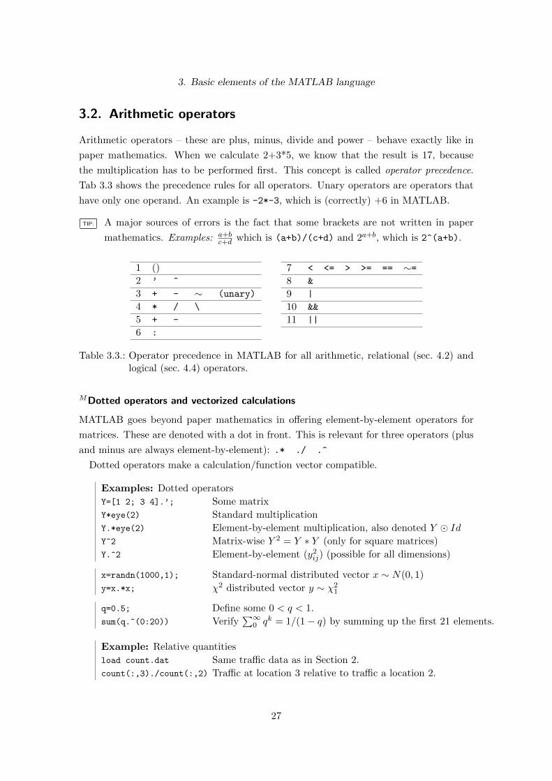
3.2. Arithmetic operators
Arithmetic operators – these are plus, minus, divide and power – behave exactly like in
paper mathematics. When we calculate 2+3*5, we know that the result is 17, because
the multiplication has to be performed first. This concept is called operator precedence.
Tab 3.3 shows the precedence rules for all operators. Unary operators are operators that
have only one operand. An example is -2*-3, which is (correctly) +6 in MATLAB.
TIP: A major sources of errors is the fact that some brackets are not written in paper
mathematics. Examples: a+bc+d which is (a+b)/(c+d) and 2a+b, which is 2^(a+b).
1 ()
2 ’ ^
3 + - ∼ (unary)
4 * / \
5 + -
6 :
7 < <= > >= == ∼=8 &
9 |
10 &&
11 ||
Table 3.3.: Operator precedence in MATLAB for all arithmetic, relational (sec. 4.2) andlogical (sec. 4.4) operators.
MDotted operators and vectorized calculations
MATLAB goes beyond paper mathematics in offering element-by-element operators for
matrices. These are denoted with a dot in front. This is relevant for three operators (plus
and minus are always element-by-element): .* ./ .^
Dotted operators make a calculation/function vector compatible.
Examples: Dotted operators
Y=[1 2; 3 4].’; Some matrix
Y*eye(2) Standard multiplication
Y.*eye(2) Element-by-element multiplication, also denoted Y � IdY^2 Matrix-wise Y 2 = Y ∗ Y (only for square matrices)
Y.^2 Element-by-element (y2ij) (possible for all dimensions)
x=randn(1000,1); Standard-normal distributed vector x ∼ N(0, 1)
y=x.*x; χ2 distributed vector y ∼ χ21
q=0.5; Define some 0 < q < 1.
sum(q.^(0:20)) Verify∑∞
0 qk = 1/(1− q) by summing up the first 21 elements.
Example: Relative quantities
load count.dat Same traffic data as in Section 2.
count(:,3)./count(:,2) Traffic at location 3 relative to traffic a location 2.
27

3. Basic elements of the MATLAB language
3.3. Programs
A program is a sequence of MATLAB commands. It is saved in plain text in a file with
extension .m (also called M-File). MATLAB has a convenient editor, but you could use
any word processor to write a program. This section and PC lab 3.5 describe how to edit
program code. See chapter 12 on the important topic of planing and writing programs.
Computer programs often start as small projects and evolve into huge, confusing collec-
tions of code filling dozens of pages. It has therefore proven useful to stick to a standard
structure, like the traditional structure for MATLAB programs:
1. First line: the name of the program
2. Preamble: a short comment explaining the programAt the end of the preamble add the author’s name, e-mail and thedata
3. First block: all constants – so they are easy to find and change
4. Load and immediately convert all data.
5. Divide the main program in blocks; start each block with a comment
6. The output should be done at the end (this includes saving the results)
Figure 3.3.: Traditional structure for programs
Comments explain a program to the human reader. MATLAB ignores all text between
a percent sign (%) and the end of the line. Comments are either place at the end of each
line or in a separate line above. See chapter 12 on how to formulate comments.
A double percent sign (%%) starts a new MATLAB “cell”. These cells are a convenient
way to structure a program. Using the button, one can run programs cell-by-cell.
TIP: Practitioner’s tips for writing programs
• Save frequently and use versions after a major step, e.g. MyPrg01.m, MyPrg02.m . . .
• A clean code layout helps reading and understanding a program.
• Adhere to the rules of good programming style, see chapter 12
1 % myfirst.m
2 % This is our first program
3 % [email protected], MATLAB class 2006-2014
4
5 % Store the cost of food and beverages in two variables
6 food=50;
7 beverages=100;
8
9 % Calculate the total cost
28

3. Basic elements of the MATLAB language
10 cost=food+beverages;
11 disp(cost)
3.4. Functions
3.4.1. Built-in functions
The built-in functions of MATLAB implement most standard mathematical functions and
some basic statistics. Functions can be called in the command window, in programs or in
other functions.
TIP: Useful MATLAB functions are: sqrt(), exp(), log(), log10(), sign(), abs(),
round(), ceil(), floor(), sum(), min(), max(), mean(), var()
TIP: For a list of all MATLAB built-in functions, open Help/MATLAB Help and navigate
to MATLAB/Functions – By Category.
3.4.2. M Inline functions
A quick way to define a function is the so-called function handle. This permits defining a
function “on the fly” (i.e. within a program) and immediately using it. It is even possible
to define and use an inline function in the interactive mode.
Example: inline functions
sq=@(x)x^2 Create a function sq with one input argument (x)
sq(3.2) Using the function sq.
utilE=@(c,a)1-exp(-a*c) Exponential utility: u(c) = 1− e−αc.utilE(100,2)
invlog=@(x)1/log(x) Inline functions can make use of other functions
ssq=@(x,y,z)sq(x)+sq(y)+sq(z)
*Recasting functions. In economics, we are often interested in what happens to a func-
tion if we change one argument, keeping the others constant (ceteris paribus). This can be
easily done in MATLAB using inline functions. Take the exponential utility. We want to
fix the risk aversion α = 2 and make a plot of the utility as a function of the consumption.
29

3. Basic elements of the MATLAB language
Example: casting multiple-argument functions as one-argument functions
myRand=@(M)randn(10,M) Create random matrices with 10 rows and M columns.
myUtil=@(c)utilE(c,2) New function myUtil() depends only on c; α is fixed to 2.
fplot(myUtil,[0,10]) MATLAB’s fplot() requires functions of 1 argument.
fplot(utilE,[0,10]) This does not work.
Similar considerations apply for MATLAB’s numeric integration functions (to integrate
along one dimension only) or optimization functions.
3.4.3. User-defined functions
User-defined functions are plain text files and are edited and commented just as MATLAB
programs. The file name must be FunctionName.m, otherwise MATLAB will not find the
function. The first line has to start with the keyword function. Again, it has proven
useful to stick to a traditional structure when writing a function.
1. First line: function result = FunctionName (arguments)
2. Preamble – this is a short comment that explains what the functiondoes. This will be used as help text for the function.
3. Explanation of input and output parameters
4. Usage example.
5. Divide the calculation in blocks; start each block with a comment
6. Assign the function value to the variable result from the first line.
Figure 3.4.: Traditional structure for user-defined functions
Example 3. The payoff of one CHF in a bank account using continuously compounding
interest rates is a function of the interest rate r and the time t. Formally:
R : R2 → R, R(r, t) = ert (3.3)
In MATLAB, we can implement this function of two scalars as follows.
30

3. Basic elements of the MATLAB language
Example: continuously compounded interest ccinterest.mfunction y = ccinterest(r,t) Function definition% Continuously comp. return on 1 CHF Explanation also used for help ccinterest
% INPUT r 1x1 .. interest rate Explain type and meaning of input ...% t 1x1 .. time in yrs parameters (inclding units) and ...% OUTPUT y 1x1 .. payoff of the output parameters.% USAGE ccinterest(r,t) Usage example.% [email protected], 2011-09-01 Author/contact/date
y = exp(r*t); Assign a value to y, to define the outputWhat happens if we forget the semicolon?
end Optional: mark the end of function
Why use functions? This is a valid question: we could have used a simple program to for
this calculation and it would have been much shorter. However, functions provide unique
advantages: They are easily re-used and thus avoid copy-paste errors when duplicating
code. They can be easily shared among your own projects and with co-authors. They
make a program more readable by hiding “boring” code (e.g. data conversions). Finally,
they help to structure a project and make testing and finding errors easier.
Tips for writing functions
• Apply the same rules for naming variables to naming functions.
• Functions should not contain any constants to be changed. Everything that can be
changed should be an argument.
• Functions should not produce output and should not load data (exceptions apply).
• It is possible to put more than 1 function into an m-File. All but the first one are
private functions that are not accessible from outside. Useful for distributing code.
MMultiple outputs
User-defined functions can have any number (including zero) of input and output argu-
ments. For multiple output arguments, there are two solutions.
31

3. Basic elements of the MATLAB language
1 function nb = neighbours1(x)
2 % Neighbours of a number.
3 % Version with output in structure
4 % INPUT x 1x1 ... a scalar
5 % OUTPUT nb struct
6 % nb.p ... predecessor
7 % nb.s ... successor
8 nb.p=x-1;
9 nb.s=x+1;
Version 1 with output in a structure
1 function [p, s] = neighbours2(x)
2 % Neighbours of a number.
3 % Version with 2 output variables
4 % INPUT x 1x1 ... a scalar
5 % OUTPUT p 1x1 ... predecessor
6 % s 1x1 ... successor
7
8 p=x-1;
9 s=x+1;
Version 2 with two output variables
To call the first function, use myNb = neighbours1(2) and then myNb.p and myNb.s,
to call the second version use [first, second] = neighbours2(2).
Discussion. At first sight, the two functions look the same. There is, however, a big
difference in how they are used. In the second case, we need to know the order of the
output arguments. Whatever variable is first will be the predecessor, the second one the
successor. For a long list of outputs, it may be cumbersome to remember the ordering. In
the first case, we have to use the structure, which may involve a bit more coding. However,
the structure is easier to understand and helps avoid errors.
TIP: Use the terms input argument and output argument to avoid confusion.
MVectorized functions
Nearly all built-in functions can use matrix input and are executed element-by-element.
User-defined functions have to be made specifically vector-compatible. Quite a few MAT-
LAB commands require vector compatible functions, e.g. fplot (plotting), quad (numeric
integration) or lsqnonlin (optimization). Usually, we use dotted operators (sec. 3.2) to
make a function vector compatible, but in a few difficult cases, we have to rewrite the
function, e.g. by using for-loops.
Example: matrix/vector-compatible functionsa=[1 3 5] An input vectorlog(a) The logarithm is applied to each element of asq(a) Applying our function to a vector produces an error message.sq2=@(x)x.^2 Just add one dot to vectorize it.sq2(a) Works.
32

3. Basic elements of the MATLAB language
3.5. PC-Lab: The first program and the first function
Create a program from scratch in the program editor
1. Type edit newprogram.m in the command window. A message informs you that
this file does not exist and asks you whether you want to create this file. If you
accept, MATLAB creates a new program file in the current directory.
2. Now you can type a program. Note the automatic syntax coloring and indenting.
3. To run the program, use this button from the toolstrip.
4. Alternatively, enter the program’s name (newprogram.m) in the command window.
In this case, you need to save the program first.
Cell mode
1. Load celldemo.m. The first cell is always shaded yellow. This is the current cell.
2. Click into the second cell. Now the second cell is the current one and yellow.
3. To execute a program cell-by-cell, click again into the first cell and use the “Run
and Advance” button ( ) in the edit toolstrip.
4. Add a new cell at the end of the program. Press return and type %% New cell
The first function
1. Type edit neighbours.m in the command line and accept to create a new file.
2. Copy the first version of the function from page 31. Save and close it.
3. Test the function from the command line as indicated on page 31.
33

3. Basic elements of the MATLAB language
Figure 3.5.: Create a MATLAB script from the command history.
Create a program from the command history
In an evolutionary approach, you may want to start by trying a few commands in the
command window. Once satisfied, create a program directly from the Command History.
1. Select the desired commands using control-click.
2. Right-click as shown in Fig. 3.5 and select Create Script.
3. The result is a new program. Add comments and don’t forget to save.
Convert ccinterest.m to a vectorized function
It may be interesting to calculate the continuously compounded interest for several dura-
tions or several interest rates in one go, e.g. in order to produce a plot. Maybe this is
already possible ...
ccinterest(0.05, 1) One interest rate, one duration.
ccinterest(0.01:0.01:0.1, 1) Several interest rates, one duration.
ccinterest(0.05, 1:15) One rate, durations from one to 15 years.
ccinterest(0.01:0.01:0.1, 1:15) This, however, does not work. Why?
First, we have to think about the desired functionality of our vectorized function. Which
outputs should be created if (a) the rates, (b) the durations or (c) both are vectors? One
possible solution is to interpret (c) in such a way that the first rate should be combined
with the first duration, the second with the second and so on ... In this case, the solution
is to use the dotted multiplication operator, simply changing one line in the function.
y=exp(r.*t); Element-by-element multiplication.
If you make such a change, also adapt the documentation:
% INPUT r 1x1 or 1xN .. interest rate
% t 1x1 or 1xN .. time in yrs
% if r and t are vectors, the first r is evaluated at the first t and so on.
Now we can test our functionccinterest(0.01:0.01:0.1, 1:15) Still not working.
ccinterest(0.01:0.01:0.1, 1:10) This works, but does it make sense?
34

3. Basic elements of the MATLAB language
3.6. Exercises
Exercise 3.1 (Precision). For small values of d, Matlab gives zero as a result for the
following two subsequent commands: a=100+d; a-100. Find (by try and error) the largest
value of d for which this artifact occurs.
Exercise 3.2. * Some matrix operations have only limited precision. To see this, let
A =
1 2 3
4 5 6
7 9 8
and B =
2 2 4
1 3 5
2 4 8
.
(a) Verify the identities for the transposed on page 172 and the trace on page 172.
(a) Verify the identities for the inverse on page 171 and the determinant on page 173.
Hint: Use format long to see possible tiny differences or check for equality using the
comparison operator ==.
Exercise 3.3 (Inline functions.). Write a short program that implements the following
utility functions as inline functions: Log utility: u(c) = ln(c), power utility: u(c, γ) =c1−γ−1
1−γ , exponential utility: u(c, α) = 1− e−αc, quadratic utility: u(c, a) = c2 − ac(a) Use the command fplot() to plot the utility functions for consumption levels between
0.5 and 10 for sensible values of the parameters.
(b) Make another plot with the power utility and values of γ of 1.1, 2, 5 and 10 as well as
the log utility. Use hold on to produce one plot with all five curves.
(c)∗ A two period utility function is defined as U(c1, c2, δ, ·) = u(c1, ·) + e−δu(c2, ·), where
u(c, ·) can be any of the above utility functions. Find a concise way to write a two-period
utility function using the power utility. How many arguments will this function take?
Exercise 3.4. Write functions that perform the following tasks using the standard struc-
ture of a function as described in in Fig. 3.4.
(a) Sum of all integers up to N. Do not use the Gauss sum formula N(N−1)2 .
(b) Calculate∑N
k=1 k2.
(c) Calculate∑N
k=1 kα using two input arguments.
Exercise 3.5 (Black-Scholes formula). The famous Black-Scholes formula for option pric-
ing takes five parameters: today’s stock price S, the strike price K, the duration t, the
interest rate r and the volatility σ. The price of a call option is then:
C = SN(d1)−Ke−rtN(d2) (3.4)
with d1 =ln(S/K)+(r+ 1
2σ2)t
σ√t
and d2 = d1 − σ√t. The symbol N(·) denotes the c.d.f. of the
standard normal distribution, with N(x) = 0.5 + 0.5 erf(x/√
2). The error function erf()
is available in MATLAB.
35

3. Basic elements of the MATLAB language
(a) Write a function StdnCdf, which calculates N() using erf(). Follow the standard
structure for user-defined functions in Fig. 3.4.
(b) Write a function BlackScholesCall that makes use of StdnCdf and calculates the
price of a call option, given S,K, t, r and σ. Choose sensible names for the variables.
Test your function with sensible values.
∗(c) Would it make sense to make BlackScholesCall vector compatible? With respect
to which input parameter(s)? Try to make your solution vector-compatible.
Hand in your solution as one file using private functions if necessary.
Exercise 3.6 (Up to you.). Find at least 5 job advertisements in your field in which
MATLAB is a requirement.
36

4. More elements of the MATLAB language
References: Hanselman and Littlefield; Getting started with MATLAB, section 4
4.1. Comparing, branching and looping
Example 4. Toss a coin: If you win, you get one Swiss Franc, else nothing. Our game has
two states: 0=loose 1=win. How can we flip a coin in MATLAB? There is no command
for coin flipping in MATLAB, but we can use rand, which produces uniformly distributed
random numbers between 0 and 1, and apply a transformation: round(rand).
round(rand) Tosses of a coin: zero or oneround(rand(1,5)) Five tosses of a coin: zeros or ones
We want to display “win” if the state is win and “loose” else. This is our first flow
control statement.
Example: If – else – endstate=round(rand) Generate state (1=win, 0=loose)if state == 1 The logical condition is (state == 1)disp(’win’) Executed if the condition is true
else
disp(’loose’) Executed if the condition is falseend Don’t forget the end
Two things happen in the line with the if statement. First, a comparison is carried out:
Is the variable state equal to 1? Second, depending on the result of this comparison, the
program continues with different pieces of code. These two concepts will be discussed sep-
arately in the following two sections. First we discuss comparisons (relational operators),
thereafter flow control, i.e. what code to execute after a comparison.
4.2. Relational operators
Relational operators are listed in Tab. 4.1. Why are they called operators? Because they
link two variables (operands) and give a new result; just like arithmetic operators.
The image set of relational operators is quite small. It contains only true and false.
MATLAB assigns numerical values to these logical expressions:
37

4. More elements of the MATLAB language
== equal< smaller than> larger than
~= unequal<= smaller or equal>= larger or equal
Table 4.1.: Relational operators in MATLAB. Note the double equal sign (==) for equality.
1 = true 0 = false
Relational operators are matrix compatible in MATLAB. If two matrices (of equal size)
are compared, MATLAB produces a matrix of zeros and ones that contain the result of
the element-by-element comparison.
1 + 1 → 2 An arithmetic operator takes two operands to produce a result1 < 2 → true A logical operator does exactly the same.[1 3] < [2 2] The result is [1 0], because (1 < 2) is true and (3 < 2) false.
TIP: Matrix-compatible logical functions in MATLAB: all(), any(), xor(), isempty(),
issorted(), ismember(), isequal(),
Equality and floating-point numbers.
Floating-point numbers are rarely exactly (up to 10−16) equal. Instead, use a relative
difference measure.
a=11.1+12.2; b=23.3; a==b Not true because of rounding errors.
abs(a-b)/(a+b) < 1E-6 This relative condition is true.
*Calculations with relational operators
The fact that “false” and “true” have numerical values can be readily used for calculations:
to count the number of observations for which a condition is true. Or consider the following
transformation: (x)+ :=
{x if x > 0
0 if x ≤ 0, which is used in the payoff of a call option (ST −K)+.
data=randn(1,7); Produce some data.
data>0 Vector of zeros and ones for negative and positive.
dataIsPos = data>0 Save result of comparison in new variable.
sum(dataIsPos) Number of positive entries.
mean(dataIsPos) Fraction of positive entries.
data .* dataIsPos Transformation (data)+.
*Logical indexing
To extract all positive elements from the vector data, use logical indexing:
data(dataIsPos) Extract positive elements of data. Result is a shorter vector.
38

4. More elements of the MATLAB language
4.3. Flow control
4.3.1. Single choice: if – else
The if – else clause makes it possible to selectively execute parts of the code. The full
syntax is (parts in square brackets are optional):
if condition
commands ... ;
[elseif condition
commands ... ;]
[else
commands ... ;]
end
Indenting code Note that the commands between if, else and end are indented. This
is automatically done by the MATLAB editor for all commands that have an end, i.e. these
commands: if, case, for, while. If you have written your code outside MATLAB, you
can use ctr-I to automatically indent your code. Indenting is especially useful if several of
these commands are nested: for every level of indenting, there must be an end somewhere.
As long as the text is indented, we are still inside one of these clauses. Indenting also
makes the code more readable.
Matrix-valued comparisons revisited
Matrix comparisons produce matrix results. Is the if condition met, when the comparison
matrix contains some zeros and some ones? Try (help if) for the answer:
“The statements [after the if] are executed if the real part of the expression
has all non-zero elements.”
To check for equality, consider using isequal(), which produces a scalar result. Note
that isequal() also permits comparing vectors of different lengths (which always results
in false). Directly comparing vectors may lead into the following trap:
Example: some vector comparisons are neither true nor false.
a=[1 2 3]; b=[1 2 4] Define two vectors
if a==b;disp(’equal’);end We expect no output here: a 6= b.
if a~=b;disp(’unequal’);end We would have expected an output here!
a==b Why? Both expressions do not meet the
a~=b requirement of “all non-zero elements”!
isequal(a,b) Scalar result
if ~isequal(a,b);disp(’uneq.’);end This works!
39

4. More elements of the MATLAB language
4.3.2. Discrete multiple choice: switch – case
Multiple alternatives could be modeled using cascades of if – elseif – end, but this makes
the code difficult to read and evokes repeated evaluations of the condition, which may lead
to unwanted results. An alternative is the switch statement. The expression value can be
a variable, a function or even a short calculation; c1 and c2 can be numbers or vectors.
switch value
case c1commands ... ;
[case c2commands ... ;]
[otherwisecommands ... ;]
end
Example 2: test for multiple possibilitiesswitch weekday(date) Check for multiple discrete possibilities
case {2,3,4,5} MATLAB’s week starts on Sunday,disp(’Grum working days’); thus Monday is day number 2.
case 6
disp(’Home at 12:00’);
case {7,1}
disp(’Weekend!’);
otherwise
disp(’Your calendar is broken’);
end
4.3.3. Conditional loops
Consider the following statement: “While there is wine in the bottle, I go on drinking.” A
computer would do the following: drink a sip, check if there is still wine, drink a sip and
so on until the bottle is empty. In MATLAB, this is done using the while command.
while condition
commands ... ;
end
If the condition is false in the first place, the loop is never executed. If the condition is
always true (e.g. trivially while 1==1), the loop is executed an infinite number of times.
Thus, the number of executions of a while loop is between 0 and∞. The main application
are so-called iterative algorithms, that find an ever-better approximate solution for a
numerical problem (“while the solution is not good enough, continue improving”), see
section 8.
40

4. More elements of the MATLAB language
TIP: It’s a good idea to count the number of executions of a while loop and to provide
an emergency exit after, say, 1000 executions. The user can stop an infinite loop by
pressing ctr-C. MATLAB may take a few seconds to abort the loop.
Octave note: In Octave, there is an alternative loop command using repeat . . . until.
This is highly useful and very intuitive. Before using it, consider that it is not compatible
with MATLAB.
The classical structure of a while loop
Example 5. We illustrate the classical structure of a while loop with a game of three
strikes. Consider the following game: you throw three coins simultaneously. You win, if
all three coins show heads. How many tries do you need to win? How does the distribution
look like?
1. Initialize counter. tries = 0;
2. Initialize test variable outside win = 0;
the while loop.3. Perform comparison and while sum(win)<3 && tries<1000
check for the emergency exit.4. Calculate test variable. win = round(rand(1,3));
5. Increase counter. tries = tries+1;
6. Don’t forget the end end
disp(tries);
Figure 4.1.: Traditional structure for while loops, see coins.m
4.4. Two conditions: Logical operators
Consider the statement: “If you get rich and famous, I will marry you, else forget about
it.” Both conditions for marriage have to be met. The logical operators and, or combine
two conditions (logical values). They operate on a small set: {0, 1}×{0, 1} → {0, 1}. The
not operator switches between true and false. See Tab. 4.2.
& and true, if all conditions are fulfilled| or true, if at least one condition is fulfilled
~ not true ↔ false
Table 4.2.: Logical operators in MATLAB.
41

4. More elements of the MATLAB language
Example: marriage conditions
rich=round(rand) Life is ...
famous=round(rand) ... random
if rich & famous Check both conditions
disp(’I will marry you.’) Both conditions are met
else
disp(’Forget it.’) One or both conditions not met
end Both conditions are met
MShort-circuited logical operators
Consider the example 1 | <something>. This will always be true. However, it may be
quite costly to calculate <something>. For this case, MATLAB has a second version of and
and or, which have double symbols: && and ||. They are called short-circuited, because
the second expression is only evaluated if the result is not known after the first one. They
are always faster, but they only work on scalar operands.
Example: short-circuited operators
1 | sum(eig(rand(1000))) This takes quite a while to execute.
1 || sum(eig(rand(1000))) This is much faster.
0 & sum(eig(rand(1000))) This again is slow.
0 && sum(eig(rand(1000))) Much faster: we already know it will be false.
1 && sum(eig(rand(1000))) No improvement here: This can be true or false.
[0 1] && [0 0] Produces an error message as operands are not scalar.
4.5. For loops
Consider the case that you forgot to hand in your problem sets in time. You get the special
exercise (we don’t punish students) to write 100 times “I will not forget to do the problem
set.” This is a stupid, repetitive task. Can the computer do it for us? Yes – computers
are very good at stupid, repetitive tasks.
Example: special exercise
for k=1:100
disp(’I will not forget to do the problem sets’);
end
In a for-loop, the number of executions is exactly known in advance. In MATLAB,
there are a three ways to define for loops, which are all rooted in how to define a vector.
The basic syntax of the for loop is:
42

4. More elements of the MATLAB language
Figure 4.2.: You write 100 times “I will not forget to do the problem set”.
for variable = vector
commands ... ;
end
A for loop executes exactly as many times as there are elements in vector. At every
execution, the loop variable is assigned one value of vector, starting with the first one.
Most for loops look slightly different. Remember the standard ways to create a vector;
Recap: different ways to create a vector[3 5 2.2 1.7] Element by element1:10 Increments of 11:T Increments of 1 up to T (must be defined previously)1:0.5:10 Arbitrary incrementslinspace(1,10,20) Fixed number (here 20) of elements
Example: A countdown in a for loopfor k=10:-1:1 Count from ten to onedisp(k);
end
Defining a loop with a vector can be useful if you want to loop over a subset of the data
for which there is no simple rule (e.g. every second Wednesday of each month). Note that
the vector needs to be a row vector.
4.5.1. A few more things about loops
• Do not use i or j as loop variables. They are reserved for complex numbers.
• Loops can be executed in the command window. MATLAB waits until you enter
end.
43

4. More elements of the MATLAB language
• Loops are comparatively slow in MATLAB (see section 13.2.1), therefore be careful
what belongs inside the loop (e.g. execute data conversion before the loop, calculate
statistics after the loop).
• There are two special commands with for loops: break stops the execution of the
loop and leaves it, continue stops the current iteration and starts next iteration.
Both commands make understanding a program more difficult and can be easily
replaced with if or while clauses. Therefore use of these commands is discouraged.
• MATLAB allows you to change the loop variable within the loop. This usually
creates a lot of confusion and should not be done.
4.6. PC lab: Applications of for loops
diary(’forloops.txt’) Don’t forget to start a diary.
Fixed number of repetitions: Running sum of cash flows (present value)
A simple method for valuing an investment is the present value: the sum of all discounted
payments: PV =∑ CFi
(1+r)i. Assume a shopping center that is rented at a fixed rent of y
over 20 years. The interest rate be r. For-loops are perfect for implementing a sum. Note
that we need to initialize the running sum variable outside the loop.
r = 0.05; Set interest rate: 0.05 = 5%.
y = 10000; Set rent
Tmax = 20; Contract runs 20 years.
PV=0; Initialize running sum outside the loop.
for k = 1:Tmax We receive payments for Tmax years
PV = PV + y/(1+r)^k; Running sum; every year we add to PV
end Note that when entering a loop in the command window,
it will start once you enter end and press return.
disp(PV);
Fixed number of repetitions: The distribution of the game of three strikes
A small simulation: We want to produce a histogram of the number of tries until we
get three strikes. To do so, we first convert the program coins.m into a function called
coin fn.m. We then play 1000 games using a for loop and produce a plot.
44

4. More elements of the MATLAB language
N=1000; Define the number of iterations outside
for k=1:N We run the game N times
results(k)=coin_fn; Result of iteration k is stored in k-th element of results
end
[mean(results) var(results)] Some nice summary statistics
hist(results); And finally a histogram to see the distribution
Data-driven number of repetitions: Looping over data
Many empirical applications (see chapter 5) require you to inspect every data point. In
such a case, the number of executions of the for loop depends on the size of the data
matrix and should therefore be defined as such:
data=randn(100+randi(100),1) Produce a data set of random length (100 .. 200 entries)
for d=1:size(data,1) Number of loop executions = number of rows in data
if data(d)<0 Simple example of data manipulation
data(d)=0; ... negative entries are set to zero
end
end
*Nested for-loops
Sometimes we have to put a for-loop within a for-loop, for example if we want to analyze
different versions of a calculation that contains a for loop. We revisit the present value
calculation, but now with multiple different interest rates.
y = 10000; Set rent
Tmax = 20; Contract runs 20 years.
rates= 0:0.01:0.2; Possible interest rates.
for s = 1:length(rates) Loop over possible interest rates
r = rates(s); r varies between zero and twenty percent
PV(s) = 0; Initialize the s-th sum.
for k = 1: Tmax We receive payments for the next Tmax years
PV(s)=PV(s)+y/(1+r)^k; Running sum; add contribution of yeark to PVsend End the loop over the years.
end End the loop over the interest rates.
disp(PV); Output is now a vector
plot(rates,PV);
NOTE: Why do we need the variable s? At first sight, it seems we could have simplified
things by writing the first loop as for r=0.01:0.01:0.2. This is correct as long
as we do not want to save the results. As we need the results for later output, we
45

4. More elements of the MATLAB language
want to store them in the vector PV. The indices of this vector must to be integer.
Therefore we need the loop variable s that runs from 1 to length(rates).
diary off Now it is time to mail the diary to yourself.
4.7. Exercises
Exercise 4.1. Write functions that fulfill the following tasks using the standard structure
in Fig. 3.4. (a) Return the smaller of two input arguments. Do not use min(). (b) Return
1 if all elements of an input vector are even and 0 else.
Exercise 4.2 (Fibonacci series.). The Fibonacci series starts with {1, 1} and all sub-
sequent elements are the sum of the two previous ones. The first few elements are
{1, 1, 2, 3, 5, 8, . . . }. Write a small program or function that . . .
(a) . . . computes the Fibonacci series up to the n-th element.
(b) . . . computes all elements of the Fibonacci that are smaller than m.
(c) . . . verifies for the first l elements that the quotient of two neighboring Fibonacci
numbers approaches the golden ratio and produces a plot illustrating this fact.
Exercise 4.3. Produce N random numbers and calculate the average. Repeat this M
times so that you get M averages. Plot a histogram of these averages.
Exercise 4.4. (a) Produce a time series of N steps of a 1-dimensional random walk with
a variance of S. Produce a plot. (b) Produce a time series of N steps of a 2-dimensional
random walk. Use a variance of S for both dimensions and a correlation of 0. Produce a
2D and a 3D plot.
Exercise 4.5 (The Sieve of Eratosthenes). Implement the Sieve of Eratosthenes to find
all prime numbers that are smaller than N.
Exercise 4.6. (a) Calculate the sum of all squared integers up to N. (b) Calculate the
sum of all squared integers up to a maximum value of the sum of M. Display the last
integer that contributed to the sum.
Exercise 4.7 (Magic square). A magic square of size n× n has the following properties:
(1) it contains all integers from 1 to n2 exactly once, (2) the sum of all rows, columns and
diagonals are equal. Verify that MATLAB’s command magic(n) really produces a magic
square for n = 5.
46

4. More elements of the MATLAB language
Exercise 4.8. (a) Write a function dinterest, that calculates the payoff of 1 dollar with
anually discretely compounded interest. The function should have the same inputs and
outputs as ccinterest from page 31. Start with a version for scalar inputs. Test your
program with the following input: dinterest(0.05, 5.5). (b) Extend your function
dinterest to take vector input in either r or t. (c) Produce a plot of the payoff of one
dollar at 10% interest per year, with continuous and discrete compounding, for maturities
of one to 20 years, in steps of half years.
Exercise 4.9. Implement at least three different ways of a list of the numbers between 1
and 1000 that can be divided by both 7 and 13.
Exercise 4.10. Take the example of the nested for loops on page 45. We want to produce
the same vector PV() as before, but calculated in a different order. (a) Change the order
of the loops, so that the loop over the payment periods (k) becomes the outer loop and
the loop over the rates (s) becomes the inner loop. Hint: You will possibly have to change
and/or rearrange a few lines of code. (b) Which of the two ways that produce the same
result is better? Write a short paragraph as a comment to your code discussing this
question.
47

5. Working with data
References: Wooldridge, section 19.3
5.1. Introduction
If an economist wants to model and explain reality, data is the gold standard of his or
her endeavor. An entire scientific field – econometrics – has evolved in order to make the
best use of data that is often faulty, incomplete, censored or based on surveys at which
people do not tell the truth. An industry has evolved to provide economists with data,
sometimes free, as from the Federal Reserve or the ECB, sometimes costing more than
$100’000. Modern computing equipment is capable of processing huge amounts of data,
such as the 1 terabyte of tick data per year, that is produced at the US stock exchanges.
Whenever we use data, we have to keep in mind that it has been recorded, processed,
transferred and converted by others. These steps produce inevitable errors. We should
never blindly trust data, even if it has been obtained for a lot of money from a renowned
source. The most important tool when working with data remains common sense.
Defintions
Data Observed/measured quantity of the study object. Usually varies with time and
from individual to individual. Data can be discerned into categorical, discrete and
continuous data.
In many econometric procedures, one part of the data (the “causes”, policy variables
or generally explanatory variables) are used to explain the other part (the “effects”,
outcomes or generally explained variables). Notation: x, xi, xt, X for explanatory
variables and y, yi, yt, Y for the explained variables. In MATLAB, it is OK to call
these variables simply X and Y if their meaning is clear.
Statistic A statistic is a function of the data, for example the following quantities: mean,
median, mode, variance, AR(1) coefficient. Note that only few statistics are model-
free, which means that most of them have to be interpreted in the context of the
underlying model. This implies that our inference can be completely misguided if it
is based on a statistic that has been calculated using a mis-specified model.
48

5. Working with data
Parameter Quantity that specifies a certain property of a model. Parameter estimation is
the process of finding the parameter that fits the data “best” according to a specific
criterion. Notation: often Greek letters such as θ (for the parameter). Estimated
parameters are often denoted with a “hat”, e.g. θ. In MATLAB it is good practice
to end the names of variables that describe estimated parameters with “-hat”, e.g.
sigmahat.
Fitted data A model can produce model-implied values for a set explained variables given
explanatory variables and parameter estimates. More formally, a model can produce
a conditional expectation for the observable quantity y given x, short y = f(θ, x).
It makes no sense to write x. Similar to estimated parameters, the name MATLAB
variables containing fitted data with “-hat”.
Envelope information. Describes the exact circumstances under which a data set has
been obtained, i.e. the source of the original data, the selection and data cleaning
procedure and the exact model specification for parameters and fitted data. It is
good MATLAB practice to add envelope information in a structure whenever saving
data (see page 191). Envelope information usually consists of:
• A reference to the input dataset (avoid duplication, do not save the input data)
• A reference to the MATLAB program (date/version) that has created this data
• The input parameters (if any), the specification of the data subset (if any) or
the model specification
• The (estimated) parameters that have been used to create fitted data
5.2. Organizing data
The audit trail is the gold standard of empirical research: as soon as we have a result, we
have to be able to show how it had been obtained, in every little step from the data to
the final number. This means we have to be able to document exactly where our data has
come from, how it has been processed (e.g. in sub-samples) and all subsequent calculations.
An audit trail also includes code, choice of (sub) model, constraints, starting values, and
assumptions. I would even go so far as saving the seed of the random number generator
for full replicability.
Creating a data structure
There is no simple solution for creating a data structure. Depending on the problem and
the nature of the data, different structures may be suitable. A few principles can help in
designing a data structure:
• Store data in its most natural format (usually how it is observed)
49

5. Working with data
• Whenever possible, store in matrix format. It is easiest to access and process.
• Avoid duplication. When a data set is used several times, its is better to reference
it and not duplicate it.
• Solve the problem of missing data. There will always be missing data. You delete
observations with missing data or interpolate to fill gaps. Both solutions have dis-
advantages.
MATLAB storage structures
• The simplest MATLAB data structure is the matrix, using the following conventions
– Time series data. One day = one row, one individual (person, firm, stock,
country) = one column, i.e. time series are always column vectors.
– Cross-sectional data. One individual = one row.
– Panel data. One individual = one column, one day = one row.
• The dataset() function is useful for working with cross-sectional data, see page 25.
• Store data with more than two dimensions (e.g. time series of covariance matrices)
in an array (see page 25)
• For non-rectangular time series data use cell arrays (see example below).
• Time series data: add a vector of timestamps. Be careful when joining two time
series (see exercise 5.3).
• The Time Series Objects and Time Series Collection Object combine time
series data with the according time stamp. See the PC lab for an example.
Example: cell arrays to organize tick dataday1=0.01*randn(100,1) Day one: 100 observationsday2=0.02*randn(150,1) Day one: 150 observations[day1 day2] Does not work ...ticks{1}=day1; Start a cell array ...ticks{2}=day2
plot(cumsum(ticks{1})) Retrieve data of first dayfor d=1:2 Loop ...rv(d)=var(ticks{d}); .. Calculate daily realized variance
end
ticks{1}(1:10) Even this is possible: first 10 observations of day 1
NOTE: Should output data such as parameter estimates or fitted data be saved or re-
calculated every time? Saving and later re-loading data can introduce inconsis-
tencies, when your saved results are based on an outdated version of your model or
your parameters. A rule of thumb is to save a calculation output only if it is very
costly to obtain (i.e. if it takes long to calculate).
50

5. Working with data
Working with calendar dates
MATLAB provides useful commands for working with calendar dates, such as: datenum(),
datestr(), datevec(), weekday(). The best way is to convert a date from any text
format (such as “2012-02-02” or “Feb 12, 2012” into a time stamp. These is simply the
number of days that have passed since January 1 in the year zero. Times of the day can
be stored as fractional time stamps. Once dates are in the time stamp using datenum(),
they can be easily added and subtracted. A useful command for plots is datetick().
Example: working with calendar datesdatestr(0) The start of all time stampsmydate=’2012-09-29’ Date as a string.d=datenum(mydate) Unix date number.datestr(d) Convert back to a date.datestr(d+0.75) Fractional time stamps correspond to times of the day.datestr(d+86) Which day is 86 days after this day?peak=datenum(’2000-03-10’) The day of the NASDAQ peak.weekday(peak) On which weekday was it?
5.3. Processing data
5.3.1. Preparing a data set
Load and convert data
MATLAB provides several commands for loading data, each with its advantages and
disadvantages. It is possible to load data manually before starting a program, but it is
preferable perform the data loading inside the program to ensure consistency between the
runs of a program (everything that is done manually is a source of errors). Commands
for loading data are: xlsread(), csvread(), importdata() and textscan(), the latter
being the most powerful command.
After loading, data should be immediately converted if necessary (i.e. change of units).
Clean data
An (incomplete) checklist for cleaning data:
• Locate and read the description that came with the data
• Check measurement units (percentage/fractions, time in years/trading days/calen-
dar days) and convert if necessary
• Check for completeness (every individual on every day in the time series)
51

5. Working with data
• Find placeholders for “no data available” (often 0 or −1 or 99.99, read description).
Replace by NaN.
• Think of what to do with non-available data. Is the econometric procedure capable
of handling NaN? Will eliminating observations with NaNs introduce a bias?
• Verify selected entries form alternative sources
• Plausibility check 1: Range, summary statistics, extreme values
• Plausibility check 2: Innovations (first differences – most time series are persistent).
Watch for single (jumps) and double (outliers) spikes.
• Cross check multiple datasets: many economic quantities are correlated.
• Economic check: arbitrage relations, natural ranges (e.g. interest rates > 0)
• Elimination of “outliers” or data that carries little information
Merge data
Merging data is an everyday procedure, even the simple calculation of an excess return
requires us to merge stock and interest rate data. The following points should be observed
when merging data:
• Verify that the data is commensurate, i.e. it has a common unit of measure (for
example, all in percentage points or fractions of 1).
• Verify that the time series have common dates, see exercise 5.3.
• Use data structures for merging data of different dimensions.
NOTE: Cleaning and merging are sometimes interrelated. Cleaning data, for example, may
require a merged data set if we want to exclude days on which there have not been
observations in all relevant markets.
Calculate derived quantities
Derived quantities like returns or implied volatilities should only be calculated once a clean
and merged data set has been produced.
Save data
Data is best stored locally in a MATLAB data file.An alternative comfortable solution for
storing data for further use is a (local) database, see section 15.
TIP: Useful commands:
• sum(X), min(X), max(X), mean(X), sort(X)
• cumsum(), diff(), prod(), cumprod(), sort(), sortrows(), sign()
52

5. Working with data
• Set operations: unique(), intersect(), any(), all()
• Calculations with relational operators, see page 38
• Special conversion functions: x2mdate()
5.3.2. Creating sub-samples
Sub-samples are widely used in financial econometrics for model validation. Depending
on the purpose, different techniques are used.
In-sample v. out-of-sample
In order to verfiy whether a certain (usually parametric) model actually describes the
underlying phenomenon and does not simply (over-)fit the data, many models are tested
out of sample. The original data set is split into an “in-sample” period (usually the first
half of the data), which is used to estimate the model’s parameters. Then the model is
applied to the remaining part of the data (“out of sample”) and it is verified how much
the model fits the data better in sample than out of sample. A large difference between
the two is an indication of model misspecification and/or overfitting.
Random sub-samples
Random sub-samples are used if the amount of data is too large for the envisaged estima-
tion procedure and if a fraction (e.g. one tenth) of the observations are sufficient to obtain
a decent estimate. We randomly select a fraction of the observation, which means we can
apply all the econometric theory that is based on random sampling.
Subsampling
Sub-sampling (not to be confronted with the creation of a sub-sample) means lowering
the sampling frequency of a time series while maintaining its length, e.g. moving from
daily data to weekly data. This is usually done by dropping the surplus observations. The
opposite process, i.e. increasing the sampling frequency, entails some form of interpolation
and is discussed on page 100. The following example shows random subsampling.
Example 6. The calculation of the realised variance should be independent of the sampling
frequency. In fact, a random sub-sample should yield the same variance estimate (albeit
less efficient). One way to study this is the creation of sub-samples, where randomly
chosen observations are dropped. (It is important that the remaining observations remain
in the same order). Imagine you have a function RealizedVariance() that calculates the
realised variance over a vector of price observations. We then can use logical indexing to
create sub-samples of the price data.
53

5. Working with data
*Example: Random sub-samples with logical indexingT=size(myTick,1); number of observations in the tick datarand(10,1)>0.5 this creates a vector of zeros and ones with ca. 50% onesrand(10,1)>0.9 only ca. 10% onessize(myTick(rand(T,1)>0.5)) sub-sample with ca. 50% of observationssize(myTick(rand(T,1)>0.9)) sub-sample with ca. 10% of observationsmyTick(rand(T,1)>0.9)
RealizedVariance(myTick) Reference valueRealizedVariance(myTick(rand(T,1)>0.5))
repeat this several timesfor k=1:1000
myVariance(k)=RealizedVariance(myTick(rand(T,1)>0.5));
end
hist(myVariance) Distribution of realised variances in the sub-samples
5.4. Data sources
Free data resources
• Financial data
– finance.yahoo.com. Free financial data (click on “Historical Prices” when
viewing a ticker). Use sqq() to access the data, available at www.mathworks.
com/matlabcentral/fileexchange/4069-stock-quote-query
• Macro data
– research.stlouisfed.org/fred2. Use fred2read() to access the data, avail-
able at www.mathworks.com/matlabcentral/fileexchange/40912-fred2read
– Further central bank data www.newyorkfed.org, www.ecb.int/stats, www.
bundesbank.de/statistik, www.snb.ch/en/iabout/stat
– data.worldbank.org, use getWbData() to load the data directly into MAT-
LAB, available at www.kimjruhl.com/computing
– www.freelunch.com
• Government open data initiatives
– www.data.gov
• Other data collections
– www.quandl.com A portal for economics and finance data, with MATLAB in-
terface. You need to register to be able to use the MATLAB interface. See PC
lab.
54

5. Working with data
Commercial data providers
• www.crbtrader.com
Low-cost financial data, including futures and options, mostly US.
5.5. PC lab: Importing data
• Go to finance.yahoo.com, select the S&P500 index, download historical data
• Load the data into MATLAB using the interactive mode
• Produce a plot of the data.
Using the sqq package
• Download the sqq package from matlabcentral.com
• Install the sqq package by adding it to the MATLAB path (see page 190, “your
personal toolbox.”)
[date, close]=sqq(’MSFT’,’2004-01-01’,today)
plot(close); Stock chart.
plot(date,close) Nicer ...
datetick(’x’,10) Read the documentation of datetick
5.5.1. Working with quandl.com
Quandl is a free and powerful web repository for all sorts of numerical data, including
financial data. It provides direkt links (“APIs”) to many programming languages, includ-
ing MATLAB. If you use the quandl API for more than 50 calls per day, you need a free
registration.
Installing the quandl software
1. Go to http://www.quandl.com/help/matlab
2. Follow the information to download the MATLAB quandl package. Unzip it.
3. Save the +Quandl folder in a convenient location and add the parent folder to the MATLAB
path (see page 190). Do not add the +Quandl folder itself to the path or change its name.
4. Start MATLAB and try the following commands:myDat = Quandl.get(’QUANDL/EURCHF’) Result is a time series collection object.
plot(myDat.Rates) The time info is automatically added.
myDat.TimeInfo.Format = ’yy’; This formats the x-axis in a better way
plot(myDat.Rates) Plot again to see the result.
Registration and authentication (optional)
1. Go to www.quandl.com
55

5. Working with data
2. Click on “Sign up”. Registration is free.
3. Fill in the form
4. Once registered, log in and go to “Account” under your user name
5. Find the “API key”, a long combination of small and large letters. This is your “token”
6. In MATLAB authenticate with Quandl.auth(’your token’); (Only done once.)
Useful quandl database codes
To find a database code, search in the data browser, then locate the “permanent link” at the lower
left part of the screen and use the part of the link after https://www.quandl.com/
• Exchange rates: QUANDL/EURCHF, BAVERAGE/USD (Bitcoin)
• Stocks: GOOG/NYSE_MMM (for NYSE stocks), GOOG/NASDAQ_AAPL (for Nasdaq stocks)
• Futures: CHRIS/CME_ED1 (3 month eurodollar), CHRIS/CBOE_VX1 (VIX front month),
CHRIS/EUREX_FDAX1 (DAX), CHRIS/EUREX_FGBL1 (Bund future)
• Macro: WORLDBANK/DEU_GFDD_OE_02 (German CPI), WORLDBANK/USA_NYGDPMKTPXN (US GDP)
Some empirical work using quandl
See demo05.m
5.6. PC lab: Identifying US recessions
Go to the website of the “Federal Reserve Economic Data” at http://research.stlouisfed.org/
fred2/categories. Select National Income & Product Accounts and then GDP/GNP and finally
the series “Real Gross Domestic Product, 3 Decimal”. Read the description. Download the function
fred2read() from http://www.mathworks.com/matlabcentral/fileexchange/40912-fred2read
and add the function to the MATLAB path.
In this simple example, we now want to identify recessions, which we define as two or more
consecutive quarters of GDP drop. We do this by looking back two quarters. This means we can
only start at quarter number three.
56

5. Working with data
Load the data[calDate GDP header]=fred2read(’GDPC1’);
size(GDP); How many observations do we have?GDP(1:10) Print first few observationsdatestr(calDate(1:10)) Print the calendar dates of the first few observations.disp(header) Show the envelope information.
Indentify recessionsrecess=zeros(length(GDP),1); Initialize recessions vector ... all zeros.for t=3:length(GDP) Start loop at Q3 → minimum to look back 2 quartersif GDP(t)<GDP(t-1) && GDP(t-1)<GDP(t-2) Drop in this and the previous quarter
recess(t)=1; Then this quarter is in a recession ..recess(t-1)=1; ... and the previous one.
end
end
sum(recess) Number of quarters in recessionmean(recess) Fraction of recession quarters
Make a plotfigure Start a nice plot with grey bars for recessionsbar(calDate,recess*16000,’EdgeColor’,’none’,’FaceColor’,[0.8 0.8 0.8],’BarWidth’,1);
hold on
plot(calDate,GDP) Plot GDP over the barsdatetick(’x’,10) Change x-axis scale to calendar yearsCompare result to the official NBER recession indicator[calDateNBER recessNBER header]=fred2read(’USRECQ’);
bar(calDateNBER,recessNBER*8000,’EdgeColor’,’none’,’FaceColor’,[0.5 0.2 0.2],’BarWidth’,1);
axis([calDate(1) calDate(end) 0 16000])
The last line limits the display to 1947 and on, as USRECQhas a longer history than GDPC
5.7. Exercises
Exercise 5.1. Go back to the demo program on page 50. Write a program that produces 20 days
of tick data. The number of ticks per day should be a random number between 100 and 200. On
each day, the standard deviation of the simulated returns should be randomly drawn between 1%
and 5%. Now
(a) retrieve the first 5 returns of day 10 in the sample, (b) retrieve the last 5 returns of day
3 in the sample, (c) retrieve the last return of the last day in the sample, (d) produce a plot of
the estimated daily realized variances, (e) produce one plot showing the (overlapping) stock price
movements on day 1,10 and 20.
Exercise 5.2. Use sqq to load the stock prices of Apple Computer (AAPL) and Microsoft (MSFT)
from January 1, 1999 to yesterday. (a) Looking back over such a long sample, how large was the
realized variance of returns of holding one stock of AAPL viz. MSFT? Hint: this exercise is not
as simple as it seems. Inspect the data carefully to spot any problems. (b) Create weekly and
monthly returns for AAPL and MSFT. To create the weekly data, start from the daily data set
57

5. Working with data
and use Wednesdays if available, if not use the Tuesday of the same week and if this is also not
available, the Thursday. To create the monthly data, start again form the daily data set and use
the last day of the month for which data is available. Note: Start from the daily data set that you
have retrieved using sqq. As always, do not use any toolbox functions. (c) Calculate the realized
variance based on daily, weekly and monthly data. Which variance do you expect to be larger?
Are you surprised? (Answer these questions in one sentence as a comment in your program).
Exercise 5.3. Go to finance.yahoo.com and find the ticker symbols that yahoo uses for the S&P
500 index and the DAX. Use sqq to retrieve the values of these indices for the period from January
1, 1999 until yesterday. (a) produce a joint time series of DAX and SP500 for those days only on
which both indices were traded. To do this, write a function commontimeseries that takes two (or
better N) sets of dates and values and produces one common time series. (b) calculate the standard
deviation and the correlation separately for every calendar year in your sample. Produce a plot of
the time series of yearly standard deviations and correlations that you obtain. (c) What did you
learn about international diversification? (Answer this question in one sentence as a comment in
your program). Note: Do not use any toolbox functions and do not use MATLAB’s time series
objects.
Exercise 5.4. *Go back to the GDP/recessions par of the PC lab. Given the variable GDP, the
whole identification of recessions could be done in two lines without a loop. How?
Exercise 5.5 (Moving averages). Use sqq() and download the daily share prices for Apple Com-
puter (AAPL) from 2000-01-01 to today. Make a sensible decision which data series you use. (a)
Calculate the daily returns, make a plot and a histogram. (b) Calculate the 22-day moving average
(22 trading days) and plot both the share price and the moving average in one plot. Do not use
any toolbox functions. (c)∗ Calculate the 30-day moving average (30 calendar days) and make the
same plot as in (b).
Exercise 5.6 (Up to you.). The list of data sources in Section 5.4 is only a glimpse of the data
that is available on the web. Find at least ten reputable data sources (usually web sites), if possible
with MATLAB integration.
58

6. Linear algebra and its applicationsReferences: LeSage, Creel, Verbeek, Greene
Linear matrix algebra is an excellent tool for applied economics, as a matrix is the natural
representation of data. MATLAB is very good at handling matrices, as the matrix is the native
data type in MATLAB. This section showcases some applications of matrix algebra in economics,
econometrics and finance.
6.1. Solving systems of linear equations
Take a system of linear equations, like
2x+ 3y + 4z = 23
2x− 1y + 2z = 8
3x+ 4y + 5z = 30 (6.1)
This system can be written in matrix form as2 3 4
2 −1 2
3 4 5
xyz
=
23
8
30
(6.2)
Or shorter as
Ax = b (6.3)
The solution is then
x = A−1b (6.4)
Solving a system of equationsA=[2 3 4; 2 -1 2; 3 4 5]
b=[23 8 30].’ Column vectorx=inv(A)*b One possible solutionx=A\b Alternative with Gaussian eliminationA*x Verify resulthelp mldivide Find out more about the matrix division using \
A=[2 3 4; 2 3 4; 3 4 5]
x=inv(A)*b A has two linear dependent row vectors → error.rank(A) A does not have full rank.
59

6. Linear algebra and its applications
6.2. PC-Lab: From equation to program – OLS step-by-step
Manually programming an estimator like OLS seems to be unpractical, but we perform
this task for two reasons. First, we can watch the estimation process step-by-step, which
might help understanding it. Second,by programming a known and simple estimator, we
prepare for implementing more difficult ones.
Data preparation
load attend.txt Load data.
[n,k]=size(attend) Number of rows, number of columns.
type attend.des Check the data description and decide which part of the data to use.
Y=attend(:,2); New explained (Y ) . . . and explanatory (X) variables.
X=[ones(n,1) attend(:,1) attend(:,3) attend(:,7) ]
[n,k]=size(Y) Verify the dimensions of the sample that we are going to use.
[n,k]=size(X)
Verifying the assumptions
MLR.1 can be verified by inspecting the regression equation. MLR.2 and MLR.3 cannot
be verified. To verify MLR.4, calculate the rank of X using rank(X). See Appendix C.
OLS estimate
rank(X) Before we start, check MLR.4
rank(X.’*X) This is the same by construction: rk(A) = rk(A′A)
b=inv(X.’*X)*X.’*Y The regression coefficients (we write b for β).
u=X*b-Y The residuals (we write u for ε.)
mean(u) Not a verification of MLR.2.∑εi = 0 by construction of the estimator.
Error terms and R2
SST=(Y-mean(Y)).’*(Y-mean(Y))This is equivalent to SST =∑n
i=1(yi − y)2.
SSR=u.’*u This is equivalent to SSR =∑n
i=1 ε2i .
R2=1-SSR/SST R2 = 1− SSR/SSTsi2hat=u.’*u/(n-k-1) Estimate σ2.
sihat=sqrt(si2hat) And calculate σ.
60

6. Linear algebra and its applications
Standard errors and t-test
Xinv=inv(X.’*X) First step towards standard errors.
dXi=diag(Xinv) New command diag, self-explaining.
sdXi=sqrt(dXi) Vector of√
((X.′X)−1)jj
seb=sihat*sdXi se(βj)) = σ√
((X.′X)−1)jj
tval=tinv(.95,n-k-1) Value of the t-statistic for 90% confidence interval.
(Admittedly, tinv() is used from the statistics toolbox.)
bmin=b-tval*seb Lower bound.
bmax=b+tval*seb Upper bound.
[b seb] Output β and its standard erros.
[bmin b bmax] Output the confidence interval and the point estimate of β.
tstat=b./seb Values for the t-statistic. Note the dotted (.) division operator.
pval=2*tcdf(-abs(tstat),n-k-2)
n− k − 2 degrees of freedom, because we did not count the constant
in k.
[b seb tstat pval] The p-values and a typical output.
6.3. PC-Lab: The MATLAB Statistics Toolbox
MATLAB has a very limited number of built-in statistics functions. Many are only avail-
able in the Statistics toolbox, which is included in the student license. Serious economet-
rics, however, can only be done by manually programming or by using the Econometrics
toolbox (see next section).
diary(’statistics.txt’) Don’t forget to start a diary.
Simple estimate: regress()
If you have not yet done so, perform the data preparation steps from the previous PC lab.
b=regress(Y,X) Simple regression.
mean(X) The means of each observable in X.
mean(Y) The mean grade.
mean(X)*b This is the same as mean(Y). Why?
[b, biv]=regress(Y,X) 95% confidence intervals for β.
[biv(:,1) b biv(:,2)] Lower bound, point estimate, upper bound for each component of β.
61

6. Linear algebra and its applications
More detailed statistics: regstats()
The MATLAB command regstats() is part of the Statistics toolbox. It produces a
wide range of statistics. Its use is different from all other commands, as regstats()
automatically adds a column of ones. Thus, we need to define a different data matrix
first.
X1=[attend(:,1) attend(:,3) attend(:,7) ]
stats = regstats(Y,X1,’linear’)
The resulting stats is a data structure. To access the individual contents, use a dot.
stats.beta Regression coefficients
stats.covb Covariance of regression coefficients
stats.yhat Fitted values of the response data
stats.r Residuals
stats.mse Mean squared error
stats.rsquare R-square statistic
stats.adjrsquare Adjusted R-square statistic
stats.tstat t statistics for coefficients
stats.fstat F statistic
Note that a few components of stats are structures, again, for example tstat. Example:
to access the p-value of the t-statistics, use stats.tstat.pval
6.4. PC-lab: applications of spectral theory1
diary(’spectral.txt’) Don’t forget to start a diary.
Eigenvalues and rank
A=[2 3 4; 3 -1 2; 4 2 2]Symmetric matrix
B=[2 3 4; 2 3 4; 3 4 5]
rank(A),rank(B) One matrix has full rank, one not.
eig(A) Vector with eigenvalues.
eig(B) One or more zero eigenvalues ↔ not full rank
1See appendix A for the theory.
62

6. Linear algebra and its applications
Matrix diagonalization
[P, D] = eig(A) Eigenvectors and eigenvalues.
dot(P(:,1),P(:,2)) Columns of P are eigenvectors.
They are orthogonal, because A is symmetric.
P*D*inv(P) Reproduce A from the diagonalization.
D Some eigenvalues are negative.
sqA=P*sqrt(D)*inv(P) An application: the square root of a matrix.
sqA*sqA Verify: this is equal to A.
Choleski decomposition and correlated random numbers
Try to simulate a portfolio of two stocks i = 1, 2. Each stock return is normally distributed
with mean µi and variance σ2i , but it is further known that the returns are correlated with
a correlation coefficient ρ. For simplicity, µi = 0 and σ2i = 1.
Naive versionz1=randn(1000,1); Z1 ∼ N(0, 1)
z2=randn(1000,1); Z2 . . . same
rho=0.5; Choose some number for ρ.
x1=z1;
x2=rho*z1+(1-rho)*z2;
corr(x1,x2) Big surprise.
What went wrong? With x = Qz we can calculate the variance:
V (x) = E [xx′] = E [Qzz′Q′] = QE [zz′]Q′ = QQ′
Correct versionz = randn(1000,2); Produce z1 and z2 in one step.
Sigma=[1 0.5; 0.5 1]; Desired variance-covariance matrix.
R = chol(Sigma); Perform a Choleski decomposition.
x = z*R; Produce correctly correlated random numbers.
corr(x) Now we get what we expected.
The result does not perfectly match the desired covariance matrix, because the random
numbers produced by MATLAB are slightly correlated. We can improve the result by
taking out the initial correlations first.
63

6. Linear algebra and its applications
cor=[1 0.2 0.8; Desired correlation matrix
0.2 1 -0.2;
0.8 -0.2 1 ];
X0=randn(1000,3); Random numbers produced by MATLAB ...
corr(X0) ... are not perfectly uncorrelated.
B=chol(inv(corr(X0))); To take out initial correlations ...
X0better=X0*B; ... multiply by Choleski decomposition of inverse.
corr(X0better) Much closer to unity.
A=chol(corr); Second Choleski decomposotion introduces correlations
Xsimple=X0*A; Correlated random numbers based on simple version
Xbetter=X0better*A; Correlated random numbers based on improved version
corr(Xsimple) Simple correlated numbers are quite far from ...
corr(Xbetter) ... the desired correlation matrix.
diary off Now it is time to mail yourself your diary.
SVD decomposition
Download the program svd_foto.m and the image nash.jpg and run the program in cell
mode. Change the value of max in line 22 to different values between 10 and 300.
6.5. Exercises
Exercise 6.1. Calculate using Matlab the eigenvalues and eigenvectors of the following
matrices. Verify equation A.4. Comment on the result.
(a) A=magic(5) (b) B =
(1 1
0 1
)
Exercise 6.2. Download svd manual.m, read the code and try to understand it.
Exercise 6.3. (a) Compute the rank of at least ten random matrices of different size
(square and non-square). Can you find a rule? (b) Compute the eigenvalues of several
large square matrices created by rand(). Find a convenient graphical representation. Is
there any pattern?
Exercise 6.4. X contains a data set with the three variables EXPR,MALE and FEMALE.
EXPR stands for years of work experience, MALE is a dummy variable that is 1 if the
individual is male and FEMALE is a dummy variable that is 1 is the individual is male.
Let X =
5 0 1
7 1 0
12 0 1
3 1 0
.
64

6. Linear algebra and its applications
(a) calculate the rank of X.
(b) create three new matrices A,B and C that contain pairwise two of the three variables.
Calculate the rank of each of these matrices.
Exercise 6.5. There is no vec() function in MATLAB. Write a short program that calcu-
lates vec(A) for a matrix A of any size. Test your program with the matrix A=magic(3).
Hint: this exercise can be implemented in at least three different ways. One obvious way
is to use a for-loop (which has not yet been discussed), but there are alternatives. One is
a smart way to use the colon operator (explained in help colon), another one is to use
the command reshape() (see help).
Exercise 6.6. (a) Why did we only take four columns of attend when we declared
X=[ones(n,1) attend(:,1) attend(:,3) attend(:,7) ]? (b) Show with MATLAB,
that taking the all columns of attend would not work. (c) Find the maximum number of
variables of attend, for which we can still perform an OLS regression. Hint: there is a
very convenient way of finding linearly dependent variables in X. Try to use this method.
If you cannot find it, you can use trial and error. (d) Repeat the PC-Lab with the new,
larger data set. (e) If possible, compare the results. Did anything change?
Exercise 6.7. Take X and Y from the previous exercise. (a) Perform a full regression of
Y on X, including t-statistics. (b) Change the scale of ’homework’ such that it ranges from
0.125 to 1 instead of [12.5, 100] (i.e. not percentage points but fraction of total homeworks).
Repeat the regression. How do the β coefficients change? Does the significance change,
as well? (c) What do we learn from this exercise about interpreting β-values?
Exercise 6.8. Start with X=[ones(n,1) attend(:,1) attend(:,3) attend(:,7) ];
and Y=attend(:,2). (a) create five variables called X1 through X5, that contain the
first, second, . . . hundred observations of X. (So each Xi is different and each contains 100
observations). Create the corresponding variables Y1 through Y5. (b) Perform an OLS
regression of Y1 on X1, Y2 on X2 and so on. Compare the results and make a comment.
(c) Would it make sense to regress Y1 on X2 and so on?
Exercise 6.9. A simple extension to OLS is to discard assumption MLR.5. Heteroskedas-
ticity robust errors
V ar(β) = (X ′X)−1(X ′ΣX)(X ′X)−1
with Σ a diagonal matrix with Σii = ε2i . Repeat the PC-Lab on manual estimation with
these new error term definition. Use the diary command to document your work.
Exercise 6.10 (Up to you.). Find 3 concrete applications of linear algebra in your field.
(Examples and exercises in this chapter do not count).
65

7. Simulation-based methods
References: Greene, Appendix E.3; Brandimarte chapters 4 and 7; Judd, section 8,
Glasserman, Gilli, Maringer and Schumann, sec 6, 8
7.1. The usefulness of random numbers
The basis for every simulation is a model: a coin delivers heads with probability p and tails
with probability 1− p. If the coin is a fair coin, p is 0.5. A fair dice has a 1/6 probability
for every number. Once we have a model for the behavior of a coin, a dice, an economy
or a financial market, it is an obvious step to simulate it.
Example 7 (Rolling a dice in MATLAB). MATLAB’s rand() function produces uniformly
distributed random numbers between zero and one. For our dice, we need a discrete
distribution of integers from one to six. We can obtain this via a two step transformation:
First, we multiply by 6, which gives a uniformly distributed random number between zero
and 6. Second, rounding up to the next integer gives the desired discrete distribution.
The mathematical notation is x→ d6 · xe. In MATLAB, rolling one dice looks like this:
Example: Rolling a dice in MATLAB
dice=randi(6); Draw from discrete distribution
dice=ceil(6*rand); Draw from uniform distribution and transform
NOTE: A common error is to use round() instead of ceil(). Try round(6*rand) several
times to understand this error.
7.1.1. Producing random numbers in MATLAB
MATLAB – just as any other computer system – cannot produce truly random numbers. It
rather produces a deterministic sequence of numbers that have almost no correlation, which
is why they are called pseudo-random numbers. When MATLAB is started, the random
number generator is initialized and will always produce exactly the same deterministic
series. For some applications (e.g. to repeat a simulation experiment) this is useful, in
other cases (e.g. to enlarge a Monte Carlo sample) this must be absolutely avoided.
66

7. Simulation-based methods
Distributionprobability fn.
p.d.f.MATLAB command See ...
Bernoulli 0/1 P (0) = P (1) = 12 round(rand)
Symmetric Bernoulli P (−1) = P (1) = 12 sign(randn)
Bernoulli P (0) = q; P (1) = p rand<=p
Binomial (n,p) P (k) =
(nk
)pkqn−k sum(rand(n,1)<=p)
Uniform [0 . . . 1] U(0,1) rand
Uniform [a . . . b] U(a,b) a+(b-a)*rand
Standard normal N(0, 1) randn
Normal N(µ, σ2) sigma*randn+mu
Correlated n-dim. norm. x ∼ N(µ,Σ) mu+randn(n,1)*chol(Sigma) p. 63or mvnrnd(mu,sigma)
Table 7.1.: Random number generation in MATLAB.
To control the starting point of the sequence, one can manually set the seed of the
random number generator.
Example: random number generation
myRand=rng Obtain state of random number generator.
rand(1,5) Produce five random numbers
rand(1,5) Produce five different ones
rng(myRand); Reset the random generator
rand(1,5) Produce same five random numbers
rng(sum(100*clock)) Unique initialization.
Built-in distributions
MATLAB has three built-in distributions: the standard uniform distribution rand(), the
standard normal distribution randn() and the uniform integer distribution randi(). For
all other distributions, there are two options:
• Transform the basic distributions (see next two subsections)
• Use the random(’distribution’,A,B,C) command from the statistics toolbox,
which supports more than 20 distributions. Depending on the type of distribution,
up to three parameters A,B,C have to be provided.
67

7. Simulation-based methods
General procedure to sample from discrete distributions
A discrete distribution takes the values xi(1 ≤ i ≤ n) with probabilities pi. As usual,
pi > 0 and∑pi = 1. First we consider the simple case that xi = i.
Example 8. We want to produce random draws from the distribution
pi 0.2 0.1 0.4 0.3
xi 1 2 3 4
To produce draws from this distribution, we start with uniformly distributed random
numbers and imagine that the interval [0, 1] is divided into intervals with the lengths
p(1), p(2), . . . p(n). Our discretely distributed random number is the number of the interval
in which the uniform random number lies.
p=[0.2 0.1 0.4 0.3]; small ’p’: probabilities p(1) ... p(4)P=cumsum(p) large ’P’: cumulative probability (upper bracket values)r=rand; Save random number for next two linessum(r>P)+1 Discrete random valuer>P What did we do?for k=1:1000 As a short verification, ...dist(k)=sum(rand>P)+1; we produce 1000 random draws
end
hist(dist) And plot a histogram.
Example 9. For general values of x, we need one more step. Consider
pi 0.2 0.1 0.4 0.3
xi -1.1 0 3.2 17
Note that p and P are the same as previously. To obtain our draws, we have to define
a vector x=[-1.1 0 3.2 17]. We want to obtain x(1) with 20% probability, x(2) with
10% and so on:
x=[-1.1 0 3.2 17]; Define the vector of x-valuesx(sum(r>P)+1) A random draw
General procedure to sample from continuous distributions
The standard way to produce random numbers of any continuous distribution is to use
the inverse function of the cdf: G(y) = F−1(x). If u is uniformly random distributed on
[0, 1], then G(u) is distributed with distribution F (·).
Example 10 (Pareto distribution). The pdf of the pareto distribution is f(x) = α(1+x)1+α
for
x > 0. The cdf is accordingly F (x) = 1−(1+x)−α. Its inverse is then G(y) = (1−y)−1α−1
We can also plot the CDF from is direct and from is inverse defintions (note that the
argument Xi is used as y-values for the inverse CDF).
68

7. Simulation-based methods
alpha=5;N=1000;
parCDF=@(x,alpha) 1-(1+x).^-alpha;
parICDF=@(x,alpha) (1-x).^(-1/alpha) - 1
Xi=linspace(0,1,N);
plot(Xi, parCDF(Xi,alpha) )
hold on
plot(parICDF(Xi,alpha), Xi, ’r--’)
axis([0 3 0 1]);
We can now draw from the inverse pareto distribution
paretoDraw=@(alpha) parICDF(rand,alpha)
paretoDrawN=@(alpha,N) parICDF(rand(N,1),alpha)
The cdf of the Pareto distribution is alternatively obtained via simulation
myDraw=paretoDrawN(5,N)
plot(sort(myDraw),Xi)
7.2. Drawing from the empirical distribution
7.3. Simulating random processes
7.3.1. Simulating discrete-time random processes
A discrete-time random process is a series of random variables that are linked by a tran-
sition equation:
xt = f(xt−1) t ≥ 1 (7.1)
where f(·) is a random function. Simulating random processes is a major ingredient
in calculating statistics of this process such as expectations or estimations of the process
parameter. To do so, we need to know the functional form of f(·) and the value of x0
Brownian motion. The simplest random process is the Brownian motion:
xt = xt−1 + εt εt ∼ N(µ, σ2) (7.2)
where µ is called the drift of the process and σ2 is the variance. If µ = 0 and σ = 1,
the process is called Standard Brownian motion. The Brownian motion process has no
“memory”, i.e. the probability distribution of tomorrow depends only on the state of
today and not on the past history. This property is called the Markov property.
To simulate such a process, we need to make an assumption for x0. Note that in
MATLAB, x(0) does not exist. We need to use x(1) for x0. This is a major source of
errors.
69

7. Simulation-based methods
x(1)=0; Staring value. We use x(1) for x0, because there is no x(0).
for t=2:100 Loop over time, start with 2.
x(t)=x(t-1)+randn; Standard Brownian motion, εt ∼ N(0, 1)
end
Mean reversion: Ornstein-Uhlenbeck process.
xt+1 = xt + κ(θ − xt) + εt εt ∼ N(0, v) (7.3)
% Three Ornstein-Uhlenbeck processes
kappa=0.04; theta=0; v=0.2;
x=[5;0;-5];
for t=2:150
x(:,t)=x(:,t-1)+kappa.*(theta-x(:,t-1))+v.*randn(3,1);
end
plot(x.’)
Stochastic volatility. Models with stochastic volatility, actually consist of two processes:
one for the modelling qunatity (e.g. returns, interest rates) and one for the variance of
above quantity. When simulating such processes, we usually have to simulate both pro-
cesses step-by-step, i.e. first the variance process for t, then the main process for t before
moving to t+ 1.
Example 11 (GARCH.). The GARCH(1,1) model is usually denoted as
ln(St) = ln(St−1) + µ+ εt
εt = σtzt zt ∼ N(0, 1)
σ2t = ω + β1σ
2t−1 + α1ε
2t−1 (7.4)
Note that the σt-process depends on εt−1. As we have to know εt−1 before we can
simulate σt, we have to simulate the process in a strict order: (1) σt−1, (2) εt−1, (3) σt,
(4) εt and so on.
1 a1=0.2; b1=0.75; % Set parameters
2 w=0.05;
3 epsilon(1)=0; % Initialize epsilon-process.
70

7. Simulation-based methods
4 sigma(1)=sqrt(w);
5 for t=2:100
6 sigma(t)=sqrt(w + ...
b1*sigma(t-1)ˆ2 + ...
a1*epsilon(t-1)ˆ2);
7 epsilon(t)=sigma(t)*randn;
8 end
4 sigma2(1)=w;
5 for t=2:100
6 sigma2(t)= w + ...
b1*sigma2(t-1) + ...
a1*epsilon(t-1)ˆ2;
7 epsilon(t)=sqrt(sigma2(t))*randn;
8 end
9 S=exp(cumsum(epsilon)); % Convert from log returns to asset prices.
NOTE: There are two alternative ways to paramtetrize the GARCH process: using σ or σ2
as a variabe. Have a look at the two alternatives above. Whenever possible, it is
preferable to use the basic quantity as a variable. In this case, it is σ (sigma) in
the left case as opposed to σ2 (sigma2) in the right case. Whatever you choose, the
most important thing is to stick to your convention.
Example 12 (Discrete-time Heston model.). The transition equations for the discrete-time
Heston model (sometimes also called Feller diffusion) are:
ln(St) = ln(St−1) + µ+ σtwt wt ∼ N(0, 1)
∆σ2t = θ(ω − σ2
t−1) + ξσt−1zt zt ∼ N(0, 1)
σ2t = σ2
t−1 + θ(ω − σ2t−1) + ξσt−1zt
cov(wt, zt) = ρ (7.5)
Simulating this model is part of exercise 7.1.
7.3.2. Discretizing continuous-time processes
A continuous-time process must be discretized to a time scale of ∆t before we can simulate
it. The simples discretization scheme is the first order approximation or Euler approxi-
mation.
71
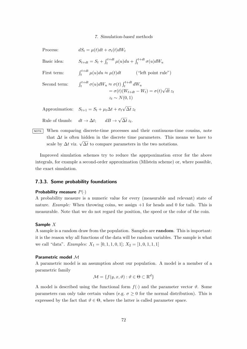
7. Simulation-based methods
Process: dSt = µ(t)dt+ σt(t)dWt
Basic idea: St+dt = St +∫ t+dtt µ(u)du+
∫ t+dtt σ(u)dWu
First term:∫ t+dtt µ(u)du ≈ µ(t)dt (“left point rule”)
Second term:∫ t+dtt σ(u)dWu ≈ σ(t)
∫ t+dtt dWu
= σ(t)(Wt+dt −Wt) = σ(t)√dt zt
zt ∼ N(0, 1)
Approximation: St+1 = St + µt∆t+ σt√
∆t zt
Rule of thumb: dt→ ∆t; dB →√
∆t zt.
NOTE: When comparing discrete-time processes and their continuous-time cousins, note
that ∆t is often hidden in the discrete time parameters. This means we have to
scale by ∆t viz.√
∆t to compare parameters in the two notations.
Improved simulation schemes try to reduce the apprpoximation error for the above
integrals, for example a second-order approximation (Milstein scheme) or, where possible,
the exact simulation.
7.3.3. Some probability foundations
Probability measure P (·)A probability measure is a numeric value for every (measurable and relevant) state of
nature. Example: When throwing coins, we assign +1 for heads and 0 for tails. This is
measurable. Note that we do not regard the position, the speed or the color of the coin.
Sample X
A sample is a random draw from the population. Samples are random. This is important:
it is the reason why all functions of the data will be random variables. The sample is what
we call “data”. Examples: X1 = [0, 1, 1, 0, 1]; X2 = [1, 0, 1, 1, 1]
Parametric model MA parametric model is an assumption about our population. A model is a member of a
parametric family
M = {f(y, x, ϑ) : ϑ ∈ Θ ⊂ Rd}
A model is described using the functional form f(·) and the parameter vector ϑ. Some
parameters can only take certain values (e.g. σ ≥ 0 for the normal distribution). This is
expressed by the fact that ϑ ∈ Θ, where the latter is called parameter space.
72

7. Simulation-based methods
Example 13 (Normal distribution). f(x, ϑ) = 1σ√
2πe−(x−µ)2
2σ2 d = 2; ϑ = (µ, σ); Θ =
(R× R+)
Statistic T
A statistic is a known function of the data X. Usually, the dimension of T is much smaller
than the dimension of X. Thus, a statistic simplifies the original data. A statistic is a
function of the data/the draw and therefore a random variable.
Closely linked to the concept of a statistic is the statistical functional, which is a func-
tion(al) of the distribution f(·). In many cases, the distinction is not made and both are
called “statistic”.
73

7. Simulation-based methods
7.4. The Monte Carlo method
The Monte Carlo method is a numerical method of solving mathematical problems by ran-
dom sampling. Simpler put, it is a method for calculating expectations. It was developed
at the Los Alamos National Laboratory, the first US atomic bomb factory to calculate
neutron diffusion in atomic bombs. The first paper about this method by Metropolis and
Ulam dates from 1949. The Monte Carlo method got its name after the city of Monte
Carlo, which is famous for its casinos, see Fig. 7.4. Note that the spinning wheel in a
casino is one of the simplest mechanical devices to produce random numbers.
Example 14. The number of points on one side of a dice be x. What is the expected value
E[x] if we throw a dice?
Theoretical calculation. E[x] = 16(1 + 2 + 3 + 4 + 5 + 6) = 3.5
Experiment. Roll a real dice 20 times, take the average. Result: µ(x) = 6920 = 3.45.
MATLAB simulation. Let MATLAB roll the dice n times and calculate the mean.
Example: A first simple simulation program dicer.m
n=100; % Good style: define n in the beginning
dice=ceil(6*rand(1,n)); % Roll 100 dice in one line
disp(dice(1:20)); % output the first few events for verification
disp(mean(dice));
3 3.2 3.4 3.6 3.8 40
500
1000
1500
2000n=100
3 3.2 3.4 3.6 3.8 40
500
1000
1500
2000n=1000
Figure 7.1.: The central limit theorem in action: Increasing n yields a more precise simu-lation result. Each simulation was repeated 10’000 times using manydice.m
Observations
• The results are somewhat close to the theoretical value, but not exact.
• Every time we repeat the simulation, we get a slightly different value.
• If we repeat the simulation many times, we can plot a distribution, see Fig. 7.1.
• If we repeat the simulation with n=1000, the distribution becomes more narrow.
74

7. Simulation-based methods
Figure 7.2.: The casino of Monte Carlo, which gave the Monte Carlo method its name.
Conclusions
• The mean is a good estimator for the expected value.
• The result of a simulation is a random variable.
• By repeating the simulations, we can assess its properties.
• If we increase n, the variance of this random variable decreases.
Two questions immediately arise. (1) Can we always use the mean as an estimator for
the expectation or have we just been lucky? (2) Does the variance of the estimation always
decrease if we increase n? By how much? The next sections will answer them.
Why simulate? Example 14 is not breathtaking. We got a result (≈ 3.5) that we already
knew, just with less precision. So is simulation any good? Not, if we are able to calculate
the theoretical values. In many cases, this is, however, not possible or not practical.
Simulation is the method of choice for stochastic problems that are either too difficult
to solve analytically or for which it is known that analytical solutions do not exist. The
only thing we usually need for a simulation is a model and the problem definition.
There are two drawbacks: first, we obtain only a specific solution for specific parameters.
Simulation methods cannot do anything about this, but we are free to run siumlations for
many different parameter sets. The second disadvantage – that our result is obtained in
the form of a random variable – can be easily mitigated by the fact that we can (a) assess
the precision of our simulation result and (b) improve it, if necessary.
75

7. Simulation-based methods
7.4.1. The method to calculate x
To calculate an unknown quantity x, we have to first construct a probabilistic model (often
quite obvious) and follow a few simple steps.
1. Find a random variable ξ such that E[ξ] = x.
Very often, this is trivial, as the desired quantity is E[ξ].
2. Produce n independent random draws ξ1, ξ2, ..., ξn.
3. Use mean as estimator for the expected value (thanks to the LLN): x = µn = 1n
∑ξi.
4. Estimate V ar(µ) (see below, MCSE) and verify if it is below the desired value. If
not, increase n accordingly and repeat steps 2 and 3.
Reflection. At first sight, step (1) may seem difficult. How could one find a suitable ξ that
fulfills the condition E[ξ] = x in order to estimate x? Fortunately, in many economics
problems, the unknown quantity is the expectation E[ξ]. In this case, the problem is
already defined in the sense of step 1.
Example 15 (Risk-neutral asset pricing). A risk-neutral agent values any asset as the
discounted expected payoff.
p0 = e−rtEQt [ξt] (7.6)
With p0 the asset price today (at time 0), r the risk-free interest rate, t the time until the
payoff is paid and ξt the payoff at time t. Notice that ξt is a random variable (we assume
we cannot predict asset returns). This problem is already formulated as in step (1) above.
7.4.2. Law of Large Numbers – LLN (Kolmogorov)
Given a sequence of n independent, identically distributed (i.i.d.) random variables ξi
with
E[ξi]
= µ (7.7)
Define the running sum Sn and the running average Xn as
Sn =n∑i=1
ξi
Xn =1
nSn =
1
n
n∑i=1
ξi (7.8)
Then
Xna.s.−→ µ (7.9)
76

7. Simulation-based methods
The law of large numbers is the basis for simulation-based methods like the Monte Carlo
method. It ensures that our simulation actually converges to the desired value. If we took
an infinite number of draws, we would get the precise value of the expectation.
7.4.3. Central limit theorem – CLT (Lindberg-Levy)
Given a sequence of n i.i.d. random variables ξi with E[ξi]
= µ, V ar[ξi]
= σ2. We first
define a new random variable Yn
Yn =Sn − nµσ√n
.
The CLT states that Yn converges in distribution to a standard normal distribution:
Yndistr−→ N(0, 1)
An alternative formulation is:
Xndistr−→ N(µ,
σ2
n) (7.10)
The CLT proves our observation that increasing n lowers the variance of the estimate.
Furthermore, we can quantify this effect: if we increase n by a factor of 100, then the
variance of the simulation will decrease by a factor of 100; the standard deviation will
decrease by a factor of 10.
The advantage of simulation based methods such as the Monte Carlo method is that
by increasing n, the variance can be made arbitrarily small. The drawback is the slow
convergence speed and the computational intensity: to achieve 10 times the precision, we
need 100 times the number of events.
The variance σ2
n is a measure for the precision of the Monte Carlo method. In theory,
it could be made arbitrarily small.
Note: The σ is the variance of the whole process. It is not always possible to calculate
σ. This σ is completely different from a possible σ-statistic in the process.
7.4.4. Monte Carlo Standard Error (MCSE)
The CLT gives the precision of the Monte Carlo method in stating that Xndistr−→ N(µ, σ
2
n ).
By increasing n, the variance decreases. But what is the value of σ2?
Example 14 continued. In some cases, it is possible to calculate σ2. In our example, ξ has a
discrete distribution with equally probable values of 1 to 6. Then V (ξ) = E[(ξ−E[ξ]
)2]=
16 [(−2.5)2 + (−1.5)2 + (−0.5)2 + 0.52 + 1.52 + 2.52] ≈ 2.92. For n = 1000, the variance of
77

7. Simulation-based methods
a Monte Carlo estimate of E[ξ] should be 2.92/1000 = 0.0029. We verify this by running
the program manydice.m with n = 1000 and calculating var(result). In a test run, we
obtain a value of 0.0028.
In the more interesting cases, in which already E[ξ] is not accessible, we cannot calculate
V [ξ] = σ2, so we have to estimate it. It would be desirable to find an estimator σ that
does not require to repeat the whole simulation several times. This estimator is the Monte
Carlo Standard Error:
σn =
√√√√ 1
n
n∑i=1
(ξi − µn)2 (7.11)
with µn = 1n
∑ξi being the Monte Carlo estimate. The index in σn indicates that the
standard error has been estimated using a sample size of n.
The MCSE is called “standard error”, because it is standardized to a sample size of
one – if we ran a Monte Carlo with n = 1, then the standard deviation of the result
would be σ. For larger samples, we apply (7.10). We get the MCSE σn with only one
additional calculation after the Monte Carlo simulation. In most cases, producing the ξi
is computationally quite intensive, so σ comes almost “for free”.
Application. The MCSE can be used to determine the sample size that is required for
some target precision. A common approach is to perform a preliminary simulation with
n = 1000 and to calculate σn. If σn is already lower than the desired precision, we are
done. If not, we can calculate the number of draws N∗ to achieve a target precision σt as
N∗ =σ2n
σ2t
(7.12)
7.4.5. Convergence, Monte Carlo versus lattice methods
Why is random sampling superior to a simple lattice/grid? The problem with a grid is
that it involves a lot of points, especially in high dimensions. A lattice of N draws in d
dimensions requires Nd calculations. To achieve a similar result with the Monte Carlo
method, only N × d calculations are required – a lot less! More precisely, the relative
errors (σ) of the two approaches scale totally differently:
εlattice(N, d) ∝ N−2d
εMC(N, d) ∝ N−12 (7.13)
78

7. Simulation-based methods
7.4.6. Extensions
General functions. The Monte Carlo method is not limited to estimating E[ξ], it can in
fact estimate E[g(ξ)] for almost any well-behaved g(·). Furthermore, we can calculate any
statistic of ξ, not only the expected value.
Variance reduction. A great deal of research has been devoted to making the Monte
Carlo method faster and thus more efficient. All these techniques aim at reducing σ2,
which in turn makes less steps necessary to obtain a certain precision. The most popular
techniques are importance sampling, in which the sample is drawn only out of the rele-
vant part of the distribution of ξ and antithetic sampling, in which pairwise negatively
correlated events reduce the overall variance. See P. Jaeckl: Monte Carlo Methods in
Finance, Wiley 2002, chapter 10.
Quasi-random numbers
Can we beat the convergence speed of the central limit theorem? Yes, with quasi-random
numbers: e.g. the Sobol sequence and the Halton sequence.
MATLAB note useful commands for creating quasi-random numbers are sobolset,
haltonset and the general command qrandstream.
7.4.7. Applications
Simulation and estimation – properties of an estimator
A large class of economic problems (e.g. asset pricing in finance) aim at explaining observed
data with a probabilistic model. In such a model, the random variable ξ depends on a
few parameters a, b, . . . . In this setting, we want the result of the Monte Carlo simulation
to be as close as possible to the data. The procedure is the following: (1) choose some
parameters a, b, . . . . (2) calculate the result of the MC. (3) compare it to the data. (4) if
the result is close enough to the data, we are done. If not, we try some other parameters
and continue with (2). In such a setting, we usually perform hundreds or thousands of
MC simulation to estimate the optimal parameter set.
Properties of many estimators (consistency, efficiency, small-sample properties) can only
be calculated using some assumptions (e.g. normality, homoskedasticity, no measurement
error on y). In the real world, these assumptions are often violated. What happens,
if the data is noisy, non-normal, heteroskedastic? This answer is often difficult to asses
analytically → Do a Monte Carlo!
79

7. Simulation-based methods
7.4.8. Four caveats
Simulation and differentiation/optimization
In these cases, we need to keep the seed the same.
Monte Carlo simulation and memory usage
Monte Carlo simulations may involve a lager number of tries, e.g. 1 million. Depending
on the application, saving all the interim values may not be necessary. This can greatly
reduce memory usage. See page 155.
Simulation and parallel computing
As we have seen, MATLAB produces exactly the same sequence of random numbers every
time it is started. This is of relevance when using the parallel computing toolbox, as
MATLAB simply launches identical copies of itself to perform parallel calculations. Each
of these copies is newly started up and would produce exactly the same sequence of random
numbers. If we want to split, say 1000 Monte Carlo simulations along 10 computers, we
have to take care that each computer has a different seed when producing the random
numbers for the simulation. For more details, see Chapter 14.
Simulate processes or distributions?
Whenever possible, we will try to avoid simulating the whole process, as this is considerably
more intensive on the computational side. It makes no sense to simulate gaussian paths
of a Black-Scholes model, when the distribution at time T is known analytically. Two
circumstances make it necessary to simulate full paths:
• If the path is explicitly needed, e.g. for path dependent (asian) options
• If the distribution of the random variable X at T = t+ τ is not known
7.5. PC-Lab: Simulation and estimation
diary(’simul.txt’) Don’t forget to start a diary.
80

7. Simulation-based methods
First steps
ceil(6*rand(1,3)) Throw three dices.
ceil(6*rand(10,3)) Throw three dices ten times.
sum(ceil(6*rand(10,3)),2) The sums of points of three dices; ten times.
a=sum(ceil(6*rand(1000,3)),2); The sums of 1000 throws of three dices.
hist(a,15) Histogram.
OLS properties
Linear model Y = βX + ε. (For more details, see Appendix C.) We run an OLS with
simulated data:
1. We choose the dimension of the model. K=3, N=200.
2. We define β = (1, 2, 5, 0.5)′. (β has dimension K + 1).
3. We produce random X-values and a random error term.
4. We calculate Y from these.
5. Next, we estimate β from our results and compare it to the initial β.
K=3, N=200 Parameters.
b=[1 2 5 0.5]’ Chosen (“real”) β. Slope parameter is 1.
X=[ones(N,1) rand(N,K)]; Include row of ones in X.
e=randn(N,1); Produce the error term.
Y=X*b+e; This is the linear model, Eq. 5.3.
[bHat, binv]=regress(Y,X) Now we estimate β.
[b bHat] Compare the results.
The OLS estimate is a random variable
e=randn(N,1); We produce a new error term ...
Y=X*b+e; ... and accordingly a new Y
[bHat2, binv]=regress(Y,X) We perform the regression a second time.
[b bHat bHat2] The results are slightly different now.
Violating OLS assumptions
Violate MLR.2: Zero conditional mean: E(ε|X) = 0
e=0.5*randn(N,1)+0.5*X(:,2);Produce a correlated error term.
Y=X*b+e; Produce a new Y with the new error term.
[bHat, binv]=regress(Y,X); We now perform a new regression.
[bHat b] Compare β to the true β. The second component – the one
which is correlated to the error term – is biased.
81

7. Simulation-based methods
Violate MLR.4: No perfect colinearity: rk(X) = k + 1
X=[ones(N,2) rand(N,K-1)]; MLR.4 is violated.
rank(X) Verify that MLR.4 is violated.
X(1:10,:) Verify what we produced.
e=randn(N,1); Produce an unbiased error term.
Y=X*b+e; Produce a new Y with the “bad” X.
[bHat, binv]=regress(Y,X); Enjoy the error message!
Time series of stock prices
A very simple assumption about the stock market: prices vary randomly, going up and
down with equal probability.
xt+1 − xtxt
=∆xtxt
= ξ with ξ ∼ N(0, σ2)
Let us simulate a time series of such a return.
s=1 Set σ = 1.
r=s*randn(100,1) Interpret as a time series of 100 returns.
plot(r) This looks pretty chaotic.
p=100+cumsum(r) This is the running sum of the stock returns. If you are
not sure what this line does, hit help cumsum.
plot(p) This plot already looks a lot like a stock chart. (It is indeed
the chart of log(xt)).
Exercise: Repeat this section several times and compare the plots. We created
various scenarios of a stock price process!
r=s*randn(100,30) Now we produce 30 scenarios at once.
p=100+cumsum(r) Stock returns.
plot(p) Plot of 30 scenarios.
Question: How much would a risk-neutral investor pay for such an asset? She would pay
the expected payoff = the expected value of the price on the last day. (We ignore interest
and discounting). We can estimate this. It is the mean of p on the last day.
mean(p(end,:)) Of course, this is a rough estimate. (Why?)
diary off Don’t forget to mail the diary to yourself.
Calculating π
We first need a probabilistic model of π. The idea is to draw random points out of the
unit square. If x2 + y2 ≤ 1, then they are part of the unit circle, else they are not. π is
82

7. Simulation-based methods
the fraction of points that are in the circle times 4.
The program circle mc.m produces the following figure:
!1 !0.8 !0.6 !0.4 !0.2 0 0.2 0.4 0.6 0.8 1!1
!0.8
!0.6
!0.4
!0.2
0
0.2
0.4
0.6
0.8
1
Option pricing using the Monte Carlo method
Run the file option sobol.m and read the comments.
7.6. Exercises
Exercise 7.1. Simulate the following stochastic processes. Use T=100, x0 = 1 and
sensible values for all other parameters. Do not use any toolbox functions. Perform a
clear before every sub-point (a), (b), . . .
(a) AR(1): xt = c+ ϕxt−1 + εt, εt ∼ N(0, σ2)
(b) AR(2): xt = c+ ϕ1xt−1 + ϕ2xt−2 + εt, εt ∼ N(0, σ2)
(c) The general AR(p) process: xt = c+∑p
i=1 ϕixt−i + εt, εt ∼ N(0, σ2).
Assume a vector ϕ of length p is given.
(d) MA(1): xt = εt + θ1εt−1, εt ∼ N(0, σ2)
(e) The ARMA(p,q) process: xt = c+ εt +∑p
i=1 ϕixt−i +∑q
k=1 θkεt−k, εt ∼ N(0, σ2).
Assume a vectors ϕ and θ of correct lengths are given.
(f∗) The Feller diffusion process, see example 12 on page 71.
Exercise 7.2. Monte Carlo basics.
(a) Produce a vector r1 with N=1000 uniformly distributed random numbers on [−0.5,+0.5].
Produce a vector r2 with N=1000 random numbers that are normally distributed
with mean zero and variance 0.5. Produce a vector r3 that is an element-by-element
sum of r1 and r2.
(b) Calculate the sample mean and sample variance of r3.
(c) Calculate analytically the mean and variance of the underlying distribution of r3.
Write the result as a comment in your program. Hint: r1 and r2 are uncorrelated.
83

7. Simulation-based methods
(d) Re-do steps (a) and (b). Do you obtain the same result? Write a short explanation
in a comment.
(e) Apply (7.11) to estimate σ. Apply (7.12) to find N∗ with σt = 0.03.
(f) Run 100 Monte Carlo simulations of r3 with N = N∗ from question (e). Calcualte
the fraction of runs in which the mean of r3 is within ±0.03 of the true value.
Compare this fraction to the theoretical value in a short comment.
(g) Continuing with the same 100 Monte Carlo simulations from (f), calcualte the frac-
tion of runs in which the variance of r3 is within ±0.03 of the true value. Compare
this fraction to the theoretical value in a short comment.
(h) Repeat the whole exercise with r1 ∼ U(−1, 1) and r2 ∼ N(0, 5).
Exercise 7.3. Numerically find the probability for scoring exactly N points with M
throws of a regular (six-sided) dice.(a) Start by producing all possible combinations and
count the winning combinations. (b) Solve the problem using a Monte Carlo simulation.
Exercise 7.4. Find the probability for the case that a) exactly two persons b) at least
two persons in a room have the same birthday (day+month). Assume that all years have
365 days and that birth dates are evenly distributed among the population. Calculate the
above probabilities for every group size from 2 to N. Make one plot with both probabilities
as a function of group size. Solve this problem using the Monte Carlo method.
Exercise 7.5 (Needle problem). Imagine you have a piece of ruled paper with lines that
are d centimeters apart. Now you drop a needle that is l ≤ d centimeters long on this
piece of paper. What is the probability that the needle will cross one of the lines? Solve
this problem via Monte Carlo simulation. (a) Calculate the probability for the special
case d = 1 and l = 0.5. (b) Produce a plot of the probability as a function of l ∈ [0, 1] for
d = 1. (c) Produce the same plot as in (b), but for l ∈ [0, 2] and d = 2. Can you find a
general rule?
Exercise 7.6. (a) Simulate the double normal distribution from exercise 3.6 using µ1 =
0, µ2 = 1, σ1 = 1, σ2 = 0.1 and calculate the skewness and kurtosis. (b∗) Simulate several
double normal distributions with 0 ≤ µi ≤ 1 and 0.1 ≤ σi ≤ 10. Calculate for each of
these distributes the skewness and kurtosis. Make a plot of skewness versus kurtosis of all
your simulations. Can you find some kind of relationship between the two?
Exercise 7.7 (Up to you.). Find 3 concrete applications of simulations in your field.
(Examples and exercises in this chapter do not count).
84

8. Algorithms
References: Mathews and Fink, section 2; Brandimarte section 2.4; Judd, section 5;
Moler, Kharab and Guenther (general and detailed), (Stanoyevitch 2005) sec 6
8.1. Nonlinear functions
8.1.1. Standard numerical problems with nonlinear functions
Standard problems in numerical mathematics for nonlinear functions f(x):
• Roots: find (all) x such that f(x) = 0
• Fixed points: find (all) x such that f(x) = x
• Inverse function: find x such that f(x) = y for a given y.
• Approximation: find a simple function g(·) such that g(x) ≈ f(x) near x0
• Minimum: find x such that f(x) is a global/local minimum (→ next section).
Closely linked to the approximation problem is a problem in dealing with data:
• Interpolation: find f(x) with x0 < x < x1, if only f(x0) and f(x1) are known
8.1.2. Properties of functions
There is no “one size fits all” numerical algorithm. Almost all methods presented here
work by assuming a certain property of the function f(·). If this condition is not fulfilled,
the numerical method may not work, or worse, it may work, but produce incorrect results.
The use of a inappropriate numerical methods is a widespread source of errors.
Before using a numerical method, verify whether all conditions are fulfilled.
Definition 1 (Global vs. local). All of the following properties may apply globally, i.e. over
the whole real line (∀x ∈ R); or locally, i.e. within an interval x ∈ [xmin, xmax] or within
a neighborhood |x− x0| < δ.
In many real world applications, there is no proof that a function has global properties.
However, it can often be shown that the desired properties are present locally. Thus we
85

8. Algorithms
x0
f(x0)
f(x1)
x1
f(x0)+f’(x0)(x1–x0)
Figure 8.1.: Left: A convex function is always above its tangent.Right: a convex function is always above its left-sided approximation.
can still use most numerical methods, provided we limit ourselves to the interval in which
the function has the required property.
Definition 2 (Increasing/decreasing). An increasing function fulfills the inequality
f(x) ≤ f(x+ ∆) for ∆ > 0 (8.1)
An alternative definition is f ′(x) ≥ 0.
For a decreasing function, the inequalities are f(x) ≥ f(x + ∆) and f ′(x) ≤ 0. A
function is called strictly increasing/decreasing, if the strict inequality holds.
Definition 3 (Monotonicity). A function that is either increasing or decreasing is called
monotonous. An alternative test for monotonicity is the horizontal line test: the graph of
the function must cross any horizontal line at most once. Strictly monotonous functions
are invertible and vice versa.
Definition 4 (Continuity). The classical definition for a continuous function is that for
every ε > 0 there exists a δ such that
f(x) + ε = f(x+ δ) (8.2)
An alternative description is that the graph of a continuous function can be drawn in one
strike, without lifting the pen from the paper.
Definition 5 (Convexity/concavity). A convex function fulfills the inequality
λf(x1) + (1− λ)f(x2) ≥ f(λx1 + (1− λ)x2) (8.3)
Alternatively, a convex function is always above its tangent (see Fig. 8.1) or f ′′ > 0. In the
multivariate case this corresponds to the condition that the Hessian matrix H = ∂2f∂xi∂xj
is
positive definite. An convex function is always above its left-sided approximation:
f(x1)− f(x0) > f ′(x0)(x1 − x0) for x1 > x0
86

8. Algorithms
For a concave function, the relation in (8.3) is inverted. It is always below its tangent,
the Hessian matrix is negative definite and f ′′ < 0. A globally convex (concave) function
has only one minimum (maximum). If f(·) is convex, then −f(·) is concave and vice versa.
Examples. The function f(x) = ex is strictly increasing and convex; f(x) = ln(x) is
strictly increasing and concave; f(x) = x2 is convex, decreasing for x < 0 and increasing
for x > 0. See fn properties.m
8.2. Polynomials, approximation and interpolation
There are good reasons why polynomials are widely used in mathematics. The are easy
to analyze and fast to evaluate, they are always continuous, differentiable and integrable,
they have simple analytical solutions to most problems (e.g. integration, differentiation)
and we have efficient methods for fitting them and finding their roots. Polynomials of
order > 1 are nonlinear functions themselves.
MATLAB commands for polynomialsa=[1 2 3]; Start with a vectorp=poly(a) Produce polynomial (x− 1)(x− 2)(x− 3)p Coefficients of x3, x2, x and 1 (see note below)polyval(p,0) Evaluate above polynomial at x = 0.polyval(p,1) If we evaluate p at one of its roots, the result is 0.x=0:0.1:4; The command polyval() is ...y=polyval(p,x); vector compatible. We can use this ...plot(x,y) for plots.r=[1 -2 1]; This is the representation of 1 · x2 − 2 · x+ 1 · 1.roots(r); Now we solve the quadratic equation x2 − 2x+ 1 = 0.roots(p) If we solve for the original polynomial, we receive again a.
NOTE: MATLAB’s notation for polynomials p=[p1 p2 p3 p4] means p1x3+p2x
2+p3x+p4.
This is exactly the other way round as in most parts of the algebraic literature, where
the notation often starts with the constant term a0 + a1x+ a2x2 + a3x
3.
Horner’s method is an efficient way to evaluate a polynomial and an example of a
useful algorithm. You can verify that MATLAB uses this method, as well by typing
edit polyval. This will open the code behind the polyval() command. The idea is
successive multiplication:
a3x3 + a2x
2 + a1x+ a0 = ((a3x+ a2)x+ a1)x+ a0
87

8. Algorithms
8.2.1. Approximation
To approximate a function f(x) means to replace it by a similar function g(x) such that
f(x) ≈ g(x) in an interval around x0. Approxmation presents us with a trade-off: g(x)
is usually easier to compute and analyze than f(x), but less precise. Thus we will only
use approximations if there is a good reason, mostly increased speed in general or the
possibility to perform parts of a calculation analytically. The latter is especially interesting
as it facilitates the analysis of a complex problem and helps to avoid some numerical
calculations altogether (e.g. replacing a numerical integration). In addition to providing
fast solutions, approximations are often used to assess their properties, (e.g. limits) by
focusing on leading terms.
By the Stone-Weierstrass theorem, any continuous function on a closed interval [a, b]
can be approximated as closely as desired using polynomials. All these properties make
polynomials such as the Taylor polynomial the obvious choice for approximations.
Error analysis. As every approximation involves some sort of error, it is useful to intro-
duce two definitions of error.
Definition 6 (Absolute error). Given the exact value x and the approximate value x , the
absolute error Eabs is:
Eabs = |x− x| (8.4)
Definition 7 (Relative error). Given x and x, the relative error Erel is
Erel =Eabs|x|
(8.5)
NOTE: It is important to use the true value x and not x as denominator in (8.5), as an
overestimated x would otherwise make the relative error seem smaller than it is.
Taylor polynomials are widely used for approximating a function. Note that these poly-
nomials are developed around the value x0 and represent a good approximation only within
some neighbourhood around it.
f(x) ≈ f(x0) +
N∑k=1
1
k!(x− x0)k f (k)(x0) (8.6)
The notation f (k)(x0) means the k-th derivative of f(·), evaluated at x0. Note that
every polynomial of order p is its own Taylor polynomial of order p.
A Taylor polynomial of order 1 is called linear approximation. The coefficients of the
Taylor polynomial are usually calculated by hand (or via the Symbolic Mathematics Tool-
88

8. Algorithms
0 1000 20001
2
3
4Nearest neighbour
0 1000 20000
0.2
0.4
0.6
0.8
1
0 1000 20001
2
3
4Linear
0 1000 20000.02
0.03
0.04
0.05
0.06
0 1000 20001
2
3
4Cubic splines
0 1000 20000
0.02
0.04
0.06
0.08
Figure 8.2.: Interpolation of the US yield curve on 2004-02-02. Duration in days. Top row:interpolated yields with observation points. Bottom row: first derivative.
box, see Sec. D.6). In the program we evaluate the polynomial.
8.2.2. Interpolation
Definition 8. The interpolation problem is to find the values of a function f(x) for x ∈[x1, xn] if only f(x1), . . . f(xN ) are known. If x should also take values outside [x1, xn],
the operation is called extrapolation.
This definition has only one requirement, namely that the interpolation function f(x)
passes through all observed points (unlike for example a regression function).
Full polynomial interpolation. One naive way to interpolate between n observed points is
a polynomial of degree (n-1). It is always possible to fit a polynomial of order p−1 through
p points(xi, f(xi)
). In MATLAB this is done using the command polyfit(x,y,n-1),
where x and y are vectors of the observed points and n is the number of points. This
solution will always exist and be continuous, but polynomial interpolation is plagued by
[overshooting], for large n, see PC lab. Also, the assumption that the data generation
function f(x) is a polynomial of high order is normally not realistic. There are two
alternatives to full polynomial interpolation.
Piecewise polynomial interpolation Piecewise interpolation makes fewer assumptions
and usually produces fewer artifacts. It uses groups of n neighbouring points to fit a
polynomial of order n−1, usually with n ≤ 3. The simplest case is n = 1, i.e. a polynomial
of order zero or a constant. This interpolation is called “nearest neighbor” interpolation.
89

8. Algorithms
As can be seen in the first column of Fig. 8.2, nearest neighbor interpolation is very close
to the original data, as it only permits observed y-values, but it is not continuous.
The next case is n = 2, i.e. a polynomial of order 1 or linear interpolation. The equation
for the linear interpolation/extrapolation is
f(x) = f(x0) +f(x1)− f(x0)
x1 − x0(x− x0) (8.7)
The second column of Fig. 8.2 reveals that the interpolation function is now continuous,
but its first derivative is not. This is due to the piecewise nature of the interpolation and
would be the same for higher-order piecewise polynomial interpolations.
Cubic spline interpolation A spline is a piecewise defined function that is smooth, i.e. it
is at least continuously differentiable. For each pair of points, a polynomial of order 3
is defined by the two points and a smooth pasting condition, i.e. that the first derivative
be continuous. The detailed derivation is a bit tedious, but MATLAB provides a ready
function for spline interpolation.
MATLAB commands for interpolationyi = interp1(x,y,xi,method)
x,y observed data pointsxi x-values of interestyi resulting interpolated valuesmode can be ’nearest’, ’linear’ or ’spline’
Transformation before interpolation
When performing an interpolation, we want to concentrate in the underlying phenomenon
and reduce any predictable interpolation error. Therefore, it is a good idea to remove all
exogenous variation before performing an interpolation. This is obtained by transforming
the data before interpolating and applying the inverse transformation on the interpolation
results. Formally:
1. Transform data: ξ0,1 = T (x0,1)
2. Interpolate ξ0,1 to obtain ξ2
3. Transform back: x2 = T−1(ξ2)
Good transformations include transforming bond prices to interest rates (removing a
duration-dependence of the interpolation error) of transforming option prices to implied
volatilities.
90
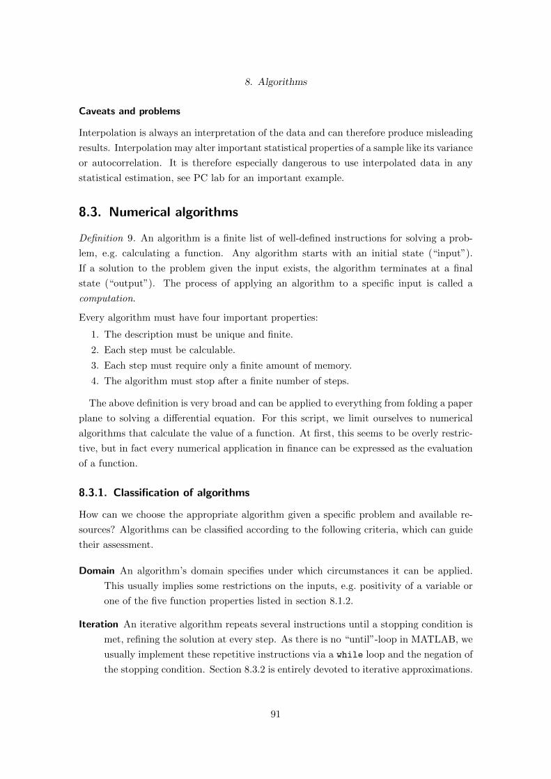
8. Algorithms
Caveats and problems
Interpolation is always an interpretation of the data and can therefore produce misleading
results. Interpolation may alter important statistical properties of a sample like its variance
or autocorrelation. It is therefore especially dangerous to use interpolated data in any
statistical estimation, see PC lab for an important example.
8.3. Numerical algorithms
Definition 9. An algorithm is a finite list of well-defined instructions for solving a prob-
lem, e.g. calculating a function. Any algorithm starts with an initial state (“input”).
If a solution to the problem given the input exists, the algorithm terminates at a final
state (“output”). The process of applying an algorithm to a specific input is called a
computation.
Every algorithm must have four important properties:
1. The description must be unique and finite.
2. Each step must be calculable.
3. Each step must require only a finite amount of memory.
4. The algorithm must stop after a finite number of steps.
The above definition is very broad and can be applied to everything from folding a paper
plane to solving a differential equation. For this script, we limit ourselves to numerical
algorithms that calculate the value of a function. At first, this seems to be overly restric-
tive, but in fact every numerical application in finance can be expressed as the evaluation
of a function.
8.3.1. Classification of algorithms
How can we choose the appropriate algorithm given a specific problem and available re-
sources? Algorithms can be classified according to the following criteria, which can guide
their assessment.
Domain An algorithm’s domain specifies under which circumstances it can be applied.
This usually implies some restrictions on the inputs, e.g. positivity of a variable or
one of the five function properties listed in section 8.1.2.
Iteration An iterative algorithm repeats several instructions until a stopping condition is
met, refining the solution at every step. As there is no “until”-loop in MATLAB, we
usually implement these repetitive instructions via a while loop and the negation of
the stopping condition. Section 8.3.2 is entirely devoted to iterative approximations.
91

8. Algorithms
Recursion A recursive algorithm invokes itself repeatedly until a stopping condition is
met. Recursive functions can be directly implemented in MATLAB, see section 8.5.
Exact or approximate Approximations are used whenever the exact solution is not avail-
able or is too slow or cumbersome to implement. Approximate algorithms usually
provide at least an upper boundary for the approximation error and in many cases
it is possible to trade precision for speed, i.e. any desired precision may be obtained
if enough computing power is available, see section 8.3.2.
Serial or parallel The problem of parallelization is not computer-specific: a tedious (man-
ual) computation performed by a single mathematician can benefit from more brain
power only if the according algorithm is parallel. Parallelization is relevant since
modern hardware has more and more calculation units. See chapter 14.
Deterministic or stochastic Given a certain input, a deterministic algorithm produces
exactly the same output at every run, while the result for a stochastic algorithm will
vary slightly. Stochastic algorithms produce by definition only approximate results,
but the precision of the result can usually be traded for computing power. Example:
The Monte Carlo method is a stochastic algorithm for calculating the expectation
of a random variable.
8.3.2. Iterative approximations and convergence
A large class of interesting algorithms are iterative approximations. They start with a
“guess” and reduce the approximation error at every iteration. This has two consequences:
first, as the error shrinks at every iteration, it can become arbitrarily small (within the
limits of the floating point representation). Second, the choice of starting value becomes
theoretically irrelevant, as a bad choice simply implies a larger starting error. The stopping
condition of such an algorithm is usually defined by a tolerance – the maximal acceptable
error – that needs to be undercut.
Make initial guess;while error > tolerance
improve guess;end
Figure 8.3.: Pseudo-code of an iterative approximation algorithm.
Mathematically, the loop can be seen as producing a series of approximations Si that
converges to the exact solution: S1, S2, . . . Sn → S. Equivalently, the sequence of relative
92

8. Algorithms
approximation errors1 εi = Si−SS can be said to converge to zero: ε1, ε2, . . . εn → 0. This
means we can borrow the concept of convergence speeds from the analysis of series.
Definition 10 (Linear convergence). A sequence εi is said to have linear convergence to 0
iflimn→∞
εn+1
εn→ q with q ∈ (0, 1).
Special cases: if q = 0 the sequence is said to have superlinear convergence,
if q = 1 the sequence is said to have sublinear convergence.
Definition 11 (Logarithmic convergence). A sequence εi that converges sublinearly (see
above) is said to converge logarithmically to zero if
εn+2 − εn+1
εn+1 − εn→ 1.
Definition 12 (Polynomial convergence). A sequence εi that converges superlinearly (see
above) is said to have polynomial convergence to zero of order p if
εn+1
εpn→ q with q ∈ [0, 1] and p > 0.
The case p = 1 is called linear convergence with εn+1 = qεn and εn = qnε1. The case p = 2
is called quadratic convergence with εn+1 = qεn2 and εn = qnε1
2n.
NOTE: Polynomial convergence of a high order is fastest, logarithmic convergence is slowest.
Example 16 (Babylonian method for calculating square roots.). This is one of the the
oldest recursive algorithms:
1. Select an arbitrary start value x0 > 0. Rule of thumb: x0 = S/2.
2. Let xn = 12
(xn−1 + S
xn−1
)3. An upper boundary for the absolute error its: en =
∣∣∣xn − Sxn
∣∣∣4. Repeat steps 2-3 while en is larger than the desired tolerance.
Notes: The algorithm even works if x0 > S. One possible interpretation of this algorithm
is that we use the arithmetic mean to approximate the geometric mean. The the error
estimate comes from the fact that the true√S must always lie between xn and S
Xn, thus
the width of the interval is the upper boundary.
1Sometimes it is easier to show convergence of absolute errors εi = (Si−S). In the limit, both statementsare equivalent and convergence rates are of the same order.
93

8. Algorithms
Let us now show the convergence of this algorithm and find its convergence speed. Note
that in the proof we use the true value√S and the true error as opposed to the upper
boundary en. First we show a simple identity:
εn =xn −
√S√
S=
xn√S− 1 (Definition of the relative error)
xn =√S · (1 + εn) (8.8)
Next we express εn+1 in terms of εn:
εn+1 =xn+1√S− 1 =
12
(xn + S
xn
)√S
− 1 =
√S · (1 + εn) + S√
S·(1+εn)
2√S
− 1
=1
2
(1 + εn +
1
1 + εn
)− 1 =
ε2n2(1 + εn)
(8.9)
Now we can evaluate εn+1/εn:
εn+1
εn=
εn2(1 + εn)
< 1 (8.10)
How fast is εn approaching zero? To assess the convergence speed, we have to go back
to (8.9) and distinguish two cases:
Case 1: big errors εn+1 ≈εn2
→ εn+1
ε1n≈ 1
2linear convergence
Case 2: small errors εn+1 ≈ε2n2
→ εn+1
ε2n≈ 1
2quadratic convergence
8.4. Some examples for iterative algorithms
The two problems of root finding and function inversion are actually very similar: root
finding can be seen as inverting a function with y = f(x) = 0, inverting a function can be
seen as finding the root of a function g(x) = f(x)− y.
8.4.1. Newton’s method for root finding
Newton’s method is an algorithm to find the root of a nonlinear function f(x), with known
first derivative, and which is monotonous on an interval. The idea is illustrated in Fig. 8.4.
1. Choose a starting value x0. This value must be in an interval around the root in
94

8. Algorithms
−0.5 0 0.5 1 1.5 2 2.5−5
0
5
10
15
20
25
30
35
40
Figure 8.4.: An illustration of Newton’s method, produced by mynewton.m.
which f(x) is monotonous.
2. Draw the tangent in (xn, yn), find the new value xn+1 where the tangent intersects
with the x-axis.
3. Redo step 2 until yn is below the precision threshold.
Note the fast convergence, which depends on the second derivative. If f(x) were a line,
the algorithm would hit the true value after one step. For moderately curved functions,
the Newton method converges very fast.
8.4.2. Bisection for inverse functions
Bisection is an algorithm to invert a function, i.e. to calculate x0 = f−1(y0) given that f()
is strictly increasing within a chosen starting interval that includes x0 (i.e. f() is locally
increasing). This monotonicity condition ensures invertability, as f : X → Y is a bijection:
for every y ∈ Y there is exactly one x ∈ X such that y = f(x).
95

8. Algorithms
0 1 2 3 4 5
−1
0
1
2
3
4
5
6
0 1 2 3 4 5
−1
0
1
2
3
4
5
6
(1) Bracketed, choose right. (2) Choose left.
0 1 2 3 4 5
−1
0
1
2
3
4
5
6
0 1 2 3 4 5
−1
0
1
2
3
4
5
6
(3) Choose left. (4) Choose right.
Figure 8.5.: Illustration of the first four steps bisection method, produced bymybisection.m. The black line indicates y0.
(1) Guess a starting interval [xL, xR] , calculate yL = f(xL) and yR = f(xR).
These intervals are shown with red lines in Fig. 8.5.
(2) If yL < y0 < yR then y0 is bracketed. If not, try a wider starting interval.
(3) Split the interval in the middle, set xM = 12(xL + xR), and calculate
yM = f(xM ). This split is shown as a dashed red line in Fig. 8.5.
(4) If y0 is in the left interval i.e. min(yL, yM ) < y0 < max(yL, yM )2, choose
it as the new interval (i.e. xR = xM ), otherwise choose the right one
(i.e. xL = xM ). The width of the x-interval has been halved.
(5) Repeat (3-4) until the upper estimate for the error, ei = |xR − xL| is
sufficiently small.
Convergence.The interval [xR − xL] shrinks by half at every iteration, thus ei → 0
and ei+1
ei= 1
2 , i.e. linear convergence. In practice, the final error after N iterations is
εN = (xR−xL)2N
. Many functions in probability (e.g. the c.d.f.) are increasing over the
whole real line and bisection can be readily applied.
Example 17 (Implied volatility). The price of a European call option is given in the Black-
2We formulate the criterion this way to make bisection work with decreasing and increasing functions.
96

8. Algorithms
Scholes formula:
C = f(X,St, σ, t, r) (8.11)
Very often, call prices are known and we want to construct a model to explain their
behaviour. Furthermore, X,St, t, r are also known precisely. This leaves σ as the obvious
choice for a free parameter. The question is: which σ would have a risk-neutral investor
have used to price this option? The σ that fulfills this equality is called the implied
volatility. The price of every vanilla option is strictly increasing in σ, so one obvious
choice is bisection.
σ = f−1(C,X, St, σ, t, r) (8.12)
NOTE: How to produce a plot of the IV-surface is shown in D.2
Bisection for root finding
If we set y = 0, bisection can be used for root finding. This is actually done in the
MATLAB function fzero().
Example 18 (Finding the implicit yield). Let us slightly change example on page 44. Let
the given quantities be the initial investment x, the annual rent y, the duration t and
the present value PV0. Which is the implicit interest rate r? It is the one for which
PV0 =∑ CFi
(1+r)ior, better, PV0 −
∑ CFi(1+r)i
= 0. Thus the problem is reduced to the root
of the difference.
We first write a function PV that calculates the present value for a given interest rate:
function result = MyPV(x, y, t, r)
% INPUT x 1x1 .... initial payment
% y 1x1 .... yearly payment
% t 1x1 .... number of years
% r 1x1 .... interest rate
result = -x; Initialize sum: value of year 0.for k = 1: t We receive payments over 20 yearsresult = result + y/(1+r)^k; Running sum; every year we add to PV
end (of function)
Next, we find the root of PV − PV0:
% impyield.m Demo of fzero
% Peter Gruber, MATLAB course 2007
x = 1000000; y= 100000; t=20;
PVstar=242000;
diff=@(r)MyPV(x,y,t,r)-PVstar;
fzero(diff,0)
97

8. Algorithms
8.5. Recursive functions
A recursive function is a function that calls itself repeatedly until a stopping condition
is met. This elegant mathematical concept can be directly translated to MATLAB, by
simply calling a function within itself. However, it is not always optimal to implement
recursive functions in MATLAB. Technically, MATLAB has to track every recursion in a
list (the “stack”) to correctly finish all the calls of the recursive function. To avoid this
list from growing to long, MATLAB limits the number of recursions. The limit can be
obtained using get(0,’RecursionLimit’) and changed using set(0,’RecursionLimit’,
N). Currently, the default limit is 500, which may be too small for many applications.
We advocate to avoid recursive functions in MATLAB. Luckily, there is always an
iterative representation for a recursive algorithm and in most cases, it will not be more
difficult to implement.
Example 19. The factorial n! = 1 · 2 · n can be recursively expressed by the factorial of
(n−1), namely n! = n ·(n−1)! with the definition 1! = 1. In MATLAB, we can implement
this as follows:
function factN = myfactorial(n)
% INPUT n 1x1 .... initial number
% OUTPUT factN 1x1 .... factorial of n
if n > 1
factN = n*myfactorial(n-1);
else
factN = 1;
end
NOTE: This function will never reach MATLAB’s recursion limit, because the factorial of 171
is already larger than realmax = 1.7977+e308, the largest number that MATLAB
can handle.
8.6. PC lab: Traps in polynomial interpolation
Horner’s methodx=1.7; Evaluate polynomial at x = 1.7
sum=p(1); Initialize algorithm. (Re-use polynomial p() from above.)for k=2:length(p); Loop over elements of the polynomial.sum=p(k)+sum*x; Taking care of the special notation in MATLAB.
end;
disp(sum)
98

8. Algorithms
p=[1/24 1/6 1/2 1 1]; Taylor polynomial of the exponential function.
MATLAB notation for f(x) ≈ 1+x+ x2
2! + x3
3! ++x4
4!x=-3:0.1:3; Some x-valuesplot(x,exp(x));hold on Plot original fn, hold on overlays approx.plot(x,polyval(p(4:end),x)); The 1st order polynomial.plot(x,polyval(p(3:end),x)); The 2nd order polynomial.plot(x,polyval(p(2:end),x)); The 3rd order polynomial.plot(x,polyval(p,x)); Full 4th order polynomial.
Polynomial interpolation
1 x=[1 2 5 6 10];2 N=length(x);3 y0=3*x;4 plot(x,y0,'k--'); hold on5 y=3*x+1*randn(1,N);6 p = polyfit(x,y,N-1);7 plot(x,y,'o');8 plot( 1:0.1:10, polyval(p, 1:0.1:10) )9 % move 1 point a bit
10 y(3)=y(3)+0.5;11 plot(x(3),y(3),'ro');12 p = polyfit(x,y,N-1);13 plot( 1:0.1:10, polyval(p, 1:0.1:10),'--')14 hold off15 %% repeat this16 % the phenomenon is called polynomial wiggle17
18 % now compare to piecewise linear interpolation19 y=3*x+1*randn(1,N);20 ytrue=3*(1:0.1:10);21 p = polyfit(x,y,N-1);22 plot(x,y0,'k--'); hold on23 plot(x,y,'o');24 plot( 1:0.1:10, polyval(p, 1:0.1:10) )25 y1=interp1(x,y,1:0.1:10,'linear');26 plot( 1:0.1:10, y1, 'r--');27 hold off28 figure29 subplot(2,1,1)30 plot(1:0.1:10,abs( polyval(p, 1:0.1:10)-ytrue) ); hold on31 plot(1:0.1:10,abs( y1-ytrue ),'r--');32 title('errors')33 subplot(2,1,2)34 hist([abs( polyval(p, 1:0.1:10)-ytrue).' abs( y1-ytrue ).' ] )
99

8. Algorithms
Tick data interpolation
1 % interpolation hf.m2 % [email protected], 2013-02-013
4 % setup5
6 % create a high-frequency data set, sampled every 15 seconds7 % 1 trading day = 8 hours = 480 mins = 1921 data points8 % for simplicity mu=0;9 sigma = 0.20 / sqrt(252) / sqrt(1921);
10
11 npoints15 = 1921; % number of points12 r0=sigma*randn(npoints15,1); % 15 sec returns13 y15 = exp(cumsum(r0)); % tick price data14 x15 = 15*(0:npoints15-1); % tick times15 plot(x15,y15) % plot16 hold on17
18 % calculate returns and annualized sigma19 retn = log(y15(2:end))-log(y15(1:end-1));20 sigmaHat15=sqrt(var(retn)*252*npoints15)21
22 % now we interpolate to 5 second intervals23 npoints5 = 1920*3+1; % number of poins24 x5 = 5*(0:npoints5-1); % new tick points25 y5 = interp1(x15,y15, x5, 'linear'); % interpolation26 plot(x5,y5,'r--') % plot exactly on top of 15s ...
interval27 retn = log(y5(2:end))-log(y5(1:end-1));28 sigmaHat5=sqrt(var(retn)*252*npoints5)29
30 % now we interpolate to 1 second intervals31 npoints1 = 1920*15+1; % number of poins32 x1 = 1*(0:npoints5-1); % new tick points33 y1 = interp1(x15,y15, x1, 'linear'); % interpolation34 retn = log(y1(2:end))-log(y1(1:end-1));35 sigmaHat1=sqrt(var(retn)*252*npoints1)36
37 % would the same thing have happend with nearest neighbour interpolation?38 y1NN = interp1(x15,y15, x1, 'nearest'); % nearst neighbour interpolation39 retn = log(y1(2:end))-log(y1(1:end-1));40 sigmaHat1NN=sqrt(var(retn)*252*npoints1)41
42 % Extra question: and if we had eliminated points?43 % try a 60s grid44 npoints60 = 1920/4+1; % number of poins45 x60 = 60*(0:npoints60-1); % new tick points46 y60 = interp1(x15,y15, x60, 'linear'); % this is called ...
"interpolation", but47 % actually we eliminate points48 plot(x60,y60,'k--') % plot is now different (need to ...
zoom in)49 retn = log(y60(2:end))-log(y60(1:end-1));50 sigmaHat60=sqrt(var(retn)*252*npoints60)
100

8. Algorithms
8.7. Exercises
Exercise 8.1 (Interpolation). Start from the code example myInterpolation.m. (a)
Calculate month-by-month forward interest rates using the different interpolation schemes.
The continuously compounded forward interest rate between horizons s and t, s < t
is f(s, t) = r(s)s−r(t)tt−s , all times are measured in years. Make a plot of the different
forward interest rate curves. (b) Add the linear interpolation scheme to the comparison.
Calculate the month-by-month forward variance swap rate, which is defined as V S(s, t) =
sqrtV S2(s)s−V S2(t)t
t−s . Make a plot of the different forward variance swap rate curves.
Exercise 8.2. (a) Write a function sqrtB that calculates the square root of any number
to a precision of 10−10 using the Babylonian algorithm. The function should have only one
input and one output argument. (This implies that you have to choose your own starting
value). (b) Write a vector-compatible version of your function that calculates the square
roots of several numbers using only one loop.
Exercise 8.3 (Inverse quantile.). Write a MATLAB function quantileInverse(), which
takes a dataset X and a fraction 0 ≤ p ≤ 1 and returns the largest number q, for which
a fraction p of the dataset is still smaller than q. Write one version of the function using
only basic MATLAB commands and one based on MATLAB’s quantile() function.
Exercise 8.4 (Kramer’s conjecture.). Take any number n ∈ N. If it is even, divide it by
2. If it is odd, multiply it by 3 and add 1. Apply the same rules to the result and so
on. The conjecture states that you will always end up at 1. Write a short program that
verifies Kramer’s conjecture for the numbers between 1 and 100, using ...
(a) an iterative function that verifies Kramer’s conjecture for one given input number.
(b) a recursive function that verifies Kramer’s conjecture for one given input number.
(c) Assuming that 0 is an even number, what would happen if we verified the conjecture
for zero? Try it and write a one-line answer as a comment to your main program.
Exercise 8.5 (Implied Volatility). Using the results from Exercise 3.5, (a) write a function
that inverts the Black Scholes formula to calculate the implied volatility of a call or put
option. Note that both call and put prices are strictly increasing functions of the volatility.
(b) For which variables would it make sense to vectorize the function? Write a vectorized
version of your function.
Exercise 8.6 (Factorial). Write an iterative version of the function myfactorial() in
Example 19.
101

9. Numeric differentiation and precision
References: Mathews and Fink, sec 6; Judd, sec 2.5, 7; Moler; Kharab and Guenther,
Gilli, Maringer and Schumann, sec 2
9.1. Introduction and mathematical background
The derivative is defined as a limit:
f ′(x) = limh→0
f (x+ h)− f (x)
h≈ ∆f(x)
∆(x)(9.1)
The problem of numeric differentiation is to find a suitable replacement for the limit
h → 0. Setting h outright zero would lead to the undefined expression 0/0. Thus the
limit must be replaced by some “very small number”. Two questions arise: What is the
optimal “small number” and is there any other room for improvements?
Example 20. We compare the numerical derivative for different values of h to the known
analytical result for f(x) = x3 with f ′ = 3x2 and plot the absolute error in Fig. 9.1.
f=@(x)x^3; x0=2; Define function and x0
truefprime=3*x^2; Define true derivativeh=10.^-(0:18); x=2; Different values of hf_prime=( f(x+h)-f(x) )./h Vector-valued calc. of all num. derivativesloglog(h,abs(f_prime-truefprime)); Log/log plot of error as function of h
9.2. The loss of precision theorem
Before we can continue the discussion of the optimal numerical differentiation, we need to
define a few concepts in the field of precision.
Theorem 1 (Loss of precision). Consider a subtraction x− y with 0 < y < x such that
10−q ≤ 1− y
x≤ 10−p (9.2)
Then at most q and at least p significant decimals are lost in the subtraction x− y.
102

9. Numeric differentiation and precision
An approximation for the number of digits lost is
q ≈ − log10(1− y
x) (9.3)
The result is usually not integer.
A few remarks:
• No precision is lost in multiplication, addition and division.
• The reason why a loss of precision occurs with the subtraction is that this is the only
operation in which two very large operands can produce a very small result. This
small number is cut off in the floating point number representation.
• If x = y, an infinite number of significant digits is lost.
• If x and y have different signs, they are actually added and there is no loss of
precision.
MATLAB example for the loss of precision theorem
x=1.23457; Define two similar numbers ...
y=1.23456; with 6 digits of precision.
format long
-log10(1-y/x) Prediction of the number of digits lost.
x-y Result has only one digit of precision, five lost.
x=2.23457; Define a very large number.
-log10(1-y/x) Not even 1 digit will be lost.
NOTE: The same holds for the number of significant bits lost: 2−a ≤ 1− yx ≤ 2−b. At most
10−20 10−15 10−10 10−5 10010−8
10−6
10−4
10−2
100
102
Figure 9.1.: Reducing h increases the precision only up to a point: there is an optimal h.
103

9. Numeric differentiation and precision
a and at least b significant bits are lost.
9.3. Tradeoff between numerical and analytical precision
How can we explain the shape of the error function in Fig. 9.1? There are two sources of
error in numerical differentiation.
Truncation error. The first is the (analytical) approximation error for h > 0. We can
use a Taylor expansion to estimate it:
f(x+ h) = f(x) + f′(x)h+
f (2)(x)
2!h2 +
f (3)(x)
3!h3 + · · · (9.4)
The error is the approximate derivative minus the true derivative:
εA =f(x+ h)− f(x)
h− f ′(x) =
f (2)(x)
2!h+
f (3)(x)
3!h2 +O(h3) (9.5)
Numerical error. The second (numerical) error stems from the loss of precision theorem,
because f(x+h) gets very close to f(x) for small h. To estimate the number of lost digits
we note that the source of the precision loss is the operation f(x+h)−f(x), independently
of the subsequent division by h.
Assume f(·) is a positive increasing function, then 0 < y = f(x) < x = f(x+ h) (if f(·)is decreasing, swap x and y). We rewrite (9.3) and insert the Taylor expansion (9.4).
q = − log10
(1− y
x
)= − log10
(x− yx
)= − log10
(f(x+ h)− f(x)
f(x)
)= − log10
(f(x) + f
′(x)h−+f (2)(x)
2! h2 + · · · − f(x)
f(x)
)
= − log10
(f′(x)h+ . . .
f(x)
)(9.6)
If q digits are lost, the corresponding absolute error 10q times the smallest number than
can be represented in the numerical system. In MATLAB this number is eps= 2.2×10⁻¹⁶.
εN = eps · 10q = eps · f(x)
f ′(x)h+O(1) (9.7)
104

9. Numeric differentiation and precision
10−20 10−15 10−10 10−5 10010−20
100
1020Analytical error
10−20 10−15 10−10 10−5 10010−20
100
1020Numerical error
10−20 10−15 10−10 10−5 10010−10
100
1010Total error
Figure 9.2.: Two sources contribute to the differentiation error: the analytical component(h→ 0) and the numerical component (loss of precision for f(x) ≈ f(x+ h)).The optimal value for h is ca. 10−8 ≈ √eps.
These errors are calculated for our example f(x) = x3 and x0 = 2 and plotted in Fig. 9.2.
To obtain the optimal h we calculate the first derivative of εA + εN with respect to h
and set it zero:∂
∂h
(εA + εN
)=f (2)(x)
2− epsf(x)
f ′(x)h2= 0 (9.8)
h∗ =√eps
√2f(x)
f (2)(x)f ′(x)(9.9)
NOTE: A rule of thumb is h =√eps · f(x) ≈ 10−8
√f(x). This rule is based on the
assumption that the expression 2f (2)(x)f ′(x)
is of order 1.
9.3.1. Higher order derivatives
Analytically, we obtain higher order derivatives by differentiating the derivative
f (n)(x) =d
dxf (n−1)(x) (9.10)
Calculating higher order derivatives numerically is a challenging problem, as each further
105

9. Numeric differentiation and precision
f = x2+y2
∇ f = 2x+2y
Figure 9.3.: The gradient points to the direction of the steepest incline.
differentiation adds to the error. If we evaluate (9.10) for n = 2 (second derivative) and
insert (9.15), we obtain an explicit formula for the second derivative:
f ′′(x) =f(x+ h)− 2f(x) + f(x− h)
h2(9.11)
In practice, this approach usually yields too large errors, see section 9.4.
9.3.2. Multivariate case
Partial derivatives pose no special problem to numeric differentiation. It makes no differ-
ence in applying (9.1) whether f(·) only depends on one x or on multiple variables.
Mixed second derivatives are obtained from the total differential:
∂2f(x0)
∂xi∂xj=f(x0 + hiei + hjej)− f(x0 − hiei + hjej)− f(x0 + hiei − hjej) + f(x0 − hiei − hjej)
4hihj
Where x0 is a vector and ei is the i−th unit vector, i.e. a vector with all zeros except
the i−th element being 1. Also note that generally hi 6= hj
Definition 13 (Gradient). The gradient of a function f(x) : Rn → R is a vector of its
partial derivatives. It is a vector that points into direction of the (locally) steepest incline
of the function, see Fig. 9.3.
grad f(x1, x2, . . . , xn) = ∇f =
∂fx1
∂fx2...∂fxn
(9.12)
The gradient is calculated component by component.
Definition 14 (Jacobian matrix). The Jacobian matrix of a function f(x) : Rn → Rm is a
matrix of its first partial derivatives. It is equal to the gradient vector for scalar functions
106

9. Numeric differentiation and precision
and is generally not square.
Jf = ∇f =
∂f1∂x1
∂f2∂x1
· · · ∂fm∂x1
∂f1∂x2
∂f2∂x2
∂fm∂x2
.... . .
...∂f1∂xn
∂f2∂xn
· · · ∂fm∂xn
(9.13)
Definition 15 (Hessian matrix). The Hessian matrix of a function f(x) : Rn → R is a
square matrix of its second partial derivatives:
Hf = ∆f =
∂2f∂x21
∂2f∂x1∂x2
· · · ∂2f∂x1∂xn
∂2f∂x2∂x1
∂2f∂x2∂x2
∂2f∂x2∂xn
.... . .
...∂2f
∂xn∂x1∂2f
∂xn∂x1· · · ∂2f
∂xn∂xn
(9.14)
This matrix is symmetric if f(·) is a continuous function. If it is positive definite, the
function is at a minimum. When calculating the Hessian matrix element by element, it
may happen that numerically ∂2f∂xi∂xj
6= ∂2f∂xj∂xi
.
Example 21 (BHHH-Estimator.). Under some regularity assumptions, the maximum like-
lihood estimator
θ = arg θmax
∑lt(θ)
in a time series environment is normally distributed as√T (θ − θ)
d→ N(0,∆−1), with
the Fisher information matrix ∆ = −E[
1T
∑ ∂2lt(θ)∂θ∂θ′
]. This sum of Hessian matrices is
numerically intensive to calculate and not guaranteed to be positive definite.
The BHHH-estimator overcomes this in a maximum likelihood setting by estimating the
Fisher Information matrix as
∆ =1
T
∑(∂lt∂θ
)(∂lt∂θ
)′This sum of outer products of gradients is much faster to calculate and guaranteed to be
positive definite. This estimator is consistent, but slightly less efficient, i.e. a few additional
iterations are the price for a more stable algorithm.
9.3.3. Improved numerical differentiation schemes
There are two routes to improve numerical differentiation: (1) higher-order algorithms
and (2) polynomial approximation.
107

9. Numeric differentiation and precision
9.4. Higher order algorithms
One way to reduce the analytical error is to use a higher order (Taylor) approximation.
The simplest improvement is the central difference method:
f ′(x) ≈ f(x+ h)− f(x− h)
2h(9.15)
this cancels out the first term in (9.5). The calculation of the optimal h becomes
∂
∂h
(εA + εN
)=
4hf (3)(x)
3! · 23− epsf(x)
f ′(x)h2= 0 (9.16)
h∗ = 3√eps 3
√12f(x)
f (3)(x)f ′(x)(9.17)
The rule of thumb for h is now larger: 3√eps · f(x) ≈ 6× 10⁻⁶ 3
√f(x).
NOTE: The central difference method is certainly more accurate, but forward differences
may still be preferable in some cases, especially when calculating the gradient or the
Jacobian matrix (see next section).
Even higher order differentiation schemes include:
f ′(x) ≈ 1
12h
(f(x− 2h)− 8f(x− h) + 8f(x+ h)− f(x+ 2h)
)(9.18)
Differential quadrature
An alternative is to approximate f(·) by a polynomial (or another set of basis functions)
and to perform a symbolic differentiation. This is especially useful when we differenti-
ate noisy data and want to ensure certain known properties (like positivity of the first
derivative).
NOTE: Do not mix up the following:
– Higher order derivatives dn
dxn f(x), e.g. the second derivative for n = 2
– Higher order algorithms are algorithms that use a better-than-necessary Taylor
approximation. For the derivative, this means they use more than n+1 function
evaluations to obtain dn
dxn f(x).
NOTE: It is not without reason that polynomial or functional approximations are widely
used as an alternative to numerical differentiation. Especially when working with
data, numerical differentiation is often too noisy.
108

9. Numeric differentiation and precision
800 900 1000 1100 1200 1300 1400 1500 1600 1700 1800−0.01
−0.005
0
0.005
0.01
0.015
Black−ScholesBreeden−LitzenbergerPolynomial approx
Figure 9.4.: Comparing the Breeden-Litzenberger formula to a symbolic differentiation ofa 8-th order polynomial and the Black-Scholes formula.
9.4.1. Higher precision and adaptive derivatives
See the DERIVESTsuite, available at http://www.mathworks.com/matlabcentral/fileexchange/
13490-adaptive-robust-numerical-differentiation. This suite also comes with an
excellent, 9-page pdf documentation.
9.5. Numeric differentiation of data
Given two vectors x = (x1, x2, . . . xn)′ and y = (f (x1) , f (x2) , . . . f (xn))′, there are two
ways to calculate the derivative by applying (9.1) and (9.15):
f ′(xm) = yi+1−yih xm = xi+xi+1
2 h = xi − xi+1
f ′(xm) = yi+1−yi−1
h xm = xi−1+xi+1
2 h = xi+1 − xi−1
(9.19)
Note that data is usually spaced quite wide, so that h � h∗. This implies that the
numerical error is of no concern. The first equation produces derivatives at points in the
middle of the original grid, the second produces points at the same grid points, but at a
lower precision. In any case, the vector of derivatives is shorter (by one or two) than the
original one.
Example 22 (The formula of Breeden and Litzenberger (1978)). A famous result is the
relation between risk-neutral probability density and option prices:
q(K) =∂2C
∂K2(9.20)
We compare three different approaches. First a double numeric differentiation of option
prices, second a symbolic differentiation of a fitted 8-th order polynomial and last a Black-
109

9. Numeric differentiation and precision
Scholes approximation. MATLAB code: ndiff breelitz.m .
9.6. PC-Lab: Higher order differentiation algortithms
• differentiation higher order.m
• differentiation higher order with noise.m
9.7. Exercises
Exercise 9.1. Reproduce the figure 9.2 for (a) f(x) = ex; (b) f(x) = ln(x); (c) f(x) = x10;
each for x0 = 5.
110

10. Optimization
References: Mathews and Fink, section 8; Brandimarte section 3; Judd, section 4; Moler,
Kharab and Guenther (general), Chong and Zak (advanced), Gilli, Maringer and Schu-
mann, sec 10-13,
Example 23. When we considered OLS, we wanted to find the “best” estimator for the
regression parameters. This problem has two steps. The first part is the question: “What
means best”? In a regression with N observations, there are N error terms εi. The
“best” estimator, however, can only be defined by one criterion. We need to find a way to
combine these N error terms. In the case of OLS, we have good reasons to choose the sum
of all squared error terms, SSE =∑
i ε2i as our criterion. We can think of the SSE as a
distance from the optimal (theoretical) case with all zero errors. A criterion that attaches
a scalar number to a generalized distance is called metric.
The second step seems to be straight forward: we need to minimize (or maximize,
depending on the definition) our criterion. The next section focuses on choosing the right
metric, while the remainder of this chapter is devoted to different techniques for finding a
minimum.
10.1. Metrics
The concept of “distance” seems to be quite natural and it seems that there is not a lot of
room for interpretation. However, even classical distances can be defined in different ways,
as Fig. 10.2 shows: While the standard distance in the two-dimensional space is just the
shortest line connecting two points, French railway passengers must frequently get from A
to Paris and from Paris to B, as there are very few trains that cross the country. Equally,
pedestrians in Manhattan can only walk along streets and avenues, making the walking
distance much longer than the distance measure in R2.
In the econometrics context, a metric is a measure for the “distance” between model
and data, between y to y, where y − y is an N -dimensional vector with N , the number
of observations, usually large. Depending on the problem, one is quite free to choose a
metric of one’s own, as the example of least squares versus least absolute deviations shows.
There are, however, four criteria, that a metric must meet.
111

10. Optimization
Definition 16. A metric is a function d(i, j) : Rn × Rn → R of two points (i, j) in Rn,
which fulfills the following four criteria:
1. Non-negativity: d(i, j) ≥ 0
Any distance is positive or zero.
2. Identity of indiscernibles: d(i, j) = 0⇔ i = j
The distance between two points is only zero, iff they are identical.
3. Symmetry: d(i, j) = d(j, i)
The distance from i to j as the same as the distance from j to i.
4. Triangle inequality: d(i, k) ≤ d(i, j) + d(j, k)
The direct path between two points is the shortest
10.2. Canonical formulation of the optimization problem
Finding the minimum, the optimum or the maximum refers to the same problem. Instead
of maximizing f(x), one can equally minimize −f(x). As already mentioned, optimizing
is either minimizing a measure of disutility(i.e. cost, error, . . . ) or maximizing a measure
of utility (i.e. profit, quality, . . . ). To simplify the exposition, we follow the literature and
discuss only the minimization problem.
0 1 2 3 4 5 6 7 8 9 100
1
2
3
4
5
6
7
y = 0.48*x + 1.3
data 1
linear
min sqared residuals
Figure 10.1.: The error term in OLS can be interpreted as distance between data andmodel.
112

10. Optimization
Standard metric in R2 Metric of the French railway system Metric of Manhattan
Figure 10.2.: Different concepts of distance, which all fulfill the definition of a metric.
10.2.1. The static minimization problem
A minimization problem is a problem of the type
minθf(θ,X) f : Rn → R, θ ∈ Θ ⊂ Rm (10.1)
where f(·) is called objective function and Θ is called feasible set. Some examples for
objective functions are given in Tab. 10.1
10.2.2. A few facts about minima
First and second derivative. If a function is twice differentiable, a (local) minimum is
found at x, where
1-dim: f ′(x) = 0 and f ′′(x) > 0
n-dim: ∂f∂x = 0 and ∂2f
∂xi∂xj(Hessian pos. definite)
(10.2)
The optimization problem can be related to finding the root of the first derivative. Some
optimization algorithms actually use this approach, but it is not always practical for two
reasons. First, the equation f ′(x) = 0 may not be straight forward to solve. Second,
if f ′(x) is not known analytically, one would have to resort to numerical differentiation,
which is computationally costly and plagued with precision problems.
mean-variance utilityleast squared errorssocial welfare function
Table 10.1.: Some objective functions
113

10. Optimization
Existence of minima. For a large class of functions, we are even guaranteed that there
exists a minimum: by the Weierstrass extreme value theorem, we know that any continuous
function on a closed interval [a, b] has both a minimum and a maximum value in this
interval.
Minimum preserving transformations. Any transformation using a strictly increasing
function preserves the location of the minimum. Any affine transformation (y = α+β · y)
with β > 0 is an example for a strictly increasing transformation. In practise, this means
it does not matter whether we minimize the sum of squared errors, the mean squared
error or the root mean squared error – all these metrics will produce the same parameter
vector θ. (We obtain, however, different results if we use mean absolute deviations or
the mean squared relative error, because they are not obtained by a strictly increasing
transformation).
Minimum preserving transformations are also used to regularise optimisation problems,
i.e. to flat objective functions that are difficult to minimise into functions with the same
minimum that are easier to handle for optimisation algorithms.
10.2.3. Classification of minimization algorithms
Different algorithms have different requirements in terms of the form of the objective
function and our knowledge about it. We can organize them along several lines:
By convexity. The most important distinction: as the name suggests, convex algorithms
work only for convex functions, while non-convex ones do not set this condition.
By use of the derivative be it explicitly (functional form of the derivative known) or
implicitly (derivative calculated numerically).
By starting values. Single starting point (most algorithms) or starting interval (e.g. grid
search, genetic algorithms)
By type of algorithm. Deterministic or stochastic. Iterative or not.
There are also two-step algorithms that combine some of the above features. Beware
that there is no “one size fits all” minimization algorithm, each of the following algorithms
has its strengths and weaknesses and works only under certain conditions. It is a major
task of the researcher to choose the best applicable algorithm.
10.3. Convex optimization
Most classical optimization algorithms and many popular MATLAB minimization com-
mands require the function under consideration to be convex. Convexity is a very restric-
114

10. Optimization
tive assumption, but it ensures the existence of a single, global minimum which permits the
creation of very efficient optimization routines. It is, however rarely met apart from some
theoretical case. While there are abundant examples in the literature of an unwarranted
use of convex optimization, it has its merits, as any function is locally convex around its
minimum. Given good starting values, convex algorithms yield fast and correct results.
10.3.1. Golden search
This algorithm works pretty much like bisection, just that the interval is not cut in half,
but divided according to the golden ratio (√
5−12 ). This very simple algorithm works only
in one dimension.
Golden SearchConvex, derivative-free, deterministic, not parallel
Advantages Disadvantages
+ Fast convergence – Can be fooled by local minima
+ Can handle discontinuity – Need good guess for starting range
+ Arbitrary precision
+/- Used for problems that have been reduced to one dimension
10.3.2. Direct search
One of the most famous direct search algorithms or n-dimensional minimization of convex
functions is the Nelder-Mead simplex algorithm. The idea is simple: try a few points,
discard the worst one and replace it by a better one. Repeat until the target precision has
been achieved. An example in 2D can be found at tinyurl.com/28ro3c. The algorithm
for n-dimensional functions looks like this:
1. Start with n + 1 points around the starting value x0, and evaluate the objective
function at each point.
2. The worst point is the one with the highest value of the objective function. This
point will be replaced.
3. Calculate the distance vector from the deleted point to the center of gravity of the
remaining points. Now three candidate points for the replacement are formed:
• Mirror point. Point the distance vector from the center of gravity of the
remaining points (i.e. away from the worst point).
• Expansion point. Just like the mirror point, but move twice the length of
the distance vector. This will increase the size of the point cloud.
115

10. Optimization
• Contraction point. Just like the mirror point, but move half the length of
the distance vector. This will shrink the size of the simplex.
4. Take the best of the three candidate points. Repeat (2-4) until the size of the point
cloud is smaller than the precision required.
Interpretation. The interplay of expansion and contraction points allows for a variable
step size: increasing swiftly far away from the minimum and decreasing close to the
minimum to enhance the algorithm’s precision.
MATLAB note. The Nelder-Mead algorithm is implemented in MATLAB’s fminsearch
command fminsearch(function_handle, first_argument, options)
Octave note. There is no fminsearch(). Instead, maximize −f(x) using mdsmax().
Nelder-Mead Simplex AlgorithmConvex, derivative-free, deterministic, parallel up to # of candiate points
Advantages Disadvantages
+ Don’t need derivative – Can be fooled by local minima
+ Can handle discontinuity – Need good guess for starting values
+ Very fast, good scaling in presence of local minima
+ Arbitrary precision
10.3.3. Gradient-based methods: steepest descent (a quasi-Newton method)
The idea is simple and convincing: if you always walk uphill you will eventually reach
the mountain top. Conversely, going downhill will lead you to the lowest point of the
valley – the minimum. The best way to do this is to follow the direction of the steepest
incline/descent. The direction of the steepest incline is given by the gradient ∇f , the
steepest descent is consequently −∇f , see Fig. 9.3.
The steepest descent algorithm is simple:
1. Start with one point x0, calculate the gradient
2. Subsequent points are obtained by subtracting a multiple of the gradient: xn+1 =
xn − s∇f(xn). Perform a grid search to find a locally optimal value of s.
3. Repeat (2) until f(xn+1) and f(xn) are within the desired tolerance
(i.e. ∇f(xn) is close to zero – near a minimum/maximum)
The optimal value for s is found in a two-step procedure. We know that a very small and
a very large number for s are not optimal (to understand why, think of the consequences of
s→ 0 and s→∞. Step 1 (bracketing): We start with an arbitrary interval for s ∈ [a, b],
116

10. Optimization
we try smaller numbers for a(a/2, a/4, a/8, . . . ) and larger numbers for b(2b, 4b, 8b, . . . )
until the result gets worse by expanding the interval. We now know that the optimal s
must be in the interval. Step 2: perform a bisection to find the optimal value of s by
evaluating f(xn − s∇f(xn)).
Interpretation. The gradient shows the direction, but how far should we go? The line
search part in the algorithm draws a line along the gradient’s direction and looks for the
optimal point along this line. This reduces the problem to a sequence one dimensional
searches, which are very fast.
Steepest descentConvex, derivative-based, deterministic, parallel up to # of variables
Advantages Disadvantages
+ Very fast – Need explicit gradient or costly numerical calc.
+ Intuitive algorithm – Cannot handle discontinuities
+/– First order approximation: fast, simple, not precise
MATLAB note. Steepest descent is implemented in the command fminunc, albeit not in
the default version. If an analytical gradient is supplied, fminunc uses it, otherwise it
calculates the gradient numerically.
More on trust region methods:
http://www.applied-mathematics.net/optimization/optimizationIntro.html
10.3.4. Advanced gradient-based methods: using the second derivative
The steepest descent is in fact a local fist-order approximation of the function. One way to
improve it is to include the second derivative (the Hessian matrix). This allows for a more
precise approximation that may be valid in a larger region around the current value, thus
permitting larger steps towards the minimum. This efficiency comes at a price: we need
to (numerically) calculate the second derivative. A whole class of so-called Quasi-Newton
methods is devoted at finding fast approximations for the Hessian matrix.
MATLAB’s fminunc and lsqnonlin are examples for these algorithms.
10.4. Nonconvex optimization
10.4.1. Grid search
This algorithm is sometimes called a “brute force” algorithm, not without reason. The idea
is find the minimum by trying all possible values. This leads us directly to the dilemma
of this method: trying all possible values will guarantee us to find the minimum, even in
117

10. Optimization
the absence of any knowledge of the objective function, but this would take an infinite
amount of time. We have to define a grid of numbers that we want to try, which limits our
search to an interval and reduces the precision. Furthermore, if we want to optimize an
n-dimensional function, a tenfold increase in precision requires an increase in the number
of grid points by a factor of 10n. This phenomenon is called the curse of dimensionality.
The algorithm is straight forward:
1. For every variable define an interval and a number of grid points (can be different
in every dimension).
2. Produce a regular grid of points within the interval(s). Evaluate the objective func-
tion at each grid point and make a list of the results.
3. Search for the lowest result in the list – this is the minimum.
Discussion. The strengths and weaknesses of grid search lie in the fact that it makes no
assumptions about the function (except the search interval). It cannot be misled by wrong
assumptions, but it cannot increase its efficiency by using such a knowledge. Furthermore,
it is the only non-iterative algorithm, which limits its potential precision. One could devise
an iterative version of grid search (search a smaller grid around the best point in the second
iteration), but this would imply making an assumption – namely smoothness – about the
function.
Example: grid searchff=@(x) x.^ 2 - x + 2;
x0 = linspace(-10,10,1000);
ytry = ff(x0);
pos = find(ytry==min(ytry));
min = x0(pos);
Grid searchNon-convex, derivative-free, deterministic, fully parallel
Advantages Disadvantages
+ Works with all functions – Slow convergence, bad scaling with precision
+ Easy to implement – Curse of dimensionality (de facto limited to 2)
– Requires starting interval
10.4.2. Combined search
Combined search is a widely used method that draws on the strengths of grid search and
direct search. The idea is to perform a grid search on a rather wide grid and to use the
(few) best grid points as starting values for a direct search. This draws from the fact
that every function is locally convex around its minimum. The implicit assumption in
118

10. Optimization
this method is that the convexity region around the minimum is larger than the spacing
of the grid points. If this is the case, combined search is the perfect method for problems
in which we have little knowledge, yet require high precision. We start by only defining
the grid and end up with arbitrary precision results form direct search.
The algorithm:
1. Perform a grid search on a comparatively wide grid.
2. Identify the n best grid points (n usually 5-10).
3. Perform n direct search operations with the best points from (2) as starting points.
4. Take the best result from (3) as minimum.
Combined searchCombined method, parallel up to # of direct searches
Advantages Disadvantages
+ The best of both worlds – Computationally intensive
10.5. Stochastic optimization
10.5.1. Differential evolution
Differential evolution (DE) is based on the principles of evolution, i.e. selection and mu-
tation. Contrary to most other algorithms, a whole population of trial vectors is tacked
from one step to the next one.
The basic version of the algorithm is:
1. Define a starting interval for each variable.
2. Start with a population of n vectors, randomly chosen out of the starting interval.
The population size is usually several times (2-10) the number of variables. Evaluate
the objective function for each population member.
3. Mutation phase: for each vector xi, find a trial vector xi by random mutation:
xi = xi + δ(xk − xl), i 6= k 6= l, 0 < δ < 2
4. Selection phase: compare the value of the objective function for each xi and xi
and retain the vector with the better value. Continue with (3) until the objective
function is below a threshold or the maximum number of steps (100 to 1000) is
reached.
There are different variations of this algorithm that use more sophisticated mutation
schemes, e.g. mutating each component of a vector independently, adding some random
noise to the mutation or forcing at least one component of the vector to remain unchanged.
119

10. Optimization
DE is not very precise, but this is outweighed by its speed and flexibility. Again, we can
employ a combined strategy to use the DE result as input for a direct search.
Discussion. The success of DE depends on choosing a good initial range for each variable
and to maintain a sufficiently large population. An interesting feature is that as the
population converges towards a minimum, the mean distance ||xk−xl|| decreases, making
the steps smaller and increasing the precision. In most practical cases, the precision of DE
increases only very slowly, thus lending hand to a combination of DE and direct search.
Differential evolutionNon-convex, derivative-free, stochastic, parallel up to # of population members
Advantages Disadvantages
+ Works with all functions – Computationally intensive
+ Comparatively fast – Requires initial interval
– Can be (rarely) fooled into local minima
– Low precision (→ combine with direct search)
10.5.2. Simulated annealing
In a nutshell, simulated annealing combines the Monte Carlo method with direct search.
This method, which was pioneered in solid state physics, solves the problem of local minima
by assigning a probability p to jump into “wrong” direction. This makes it possible to
jump out of local-minimum traps. The probability p is slowly reduced from 1 to 0 (in
physics-speak “cooled”). In the last stage, simulated annealing behaves pretty much like
direct search and homes in on the global minimum.
Simulated annealingNon-convex, derivative-free, stochastic, not parallel
Advantages Disadvantages
+ Works with all functions – Extremely slow
+ Guaranteed to find minimum – Choice of “cooling parameter” not clear
+/– Good starting parameters still help a great deal
See sim_anneal.m
10.6. Constrained optimization
A constrained optimization problem is a problem of the type:
min f(x, y) s.t. x+ y > 0
120

10. Optimization
Applications: budget constraints, economic constraints (e.g. positive interest rates),
model/legal constraints (e.g. no short selling), econometric constraints (e.g. stability of
time series process).
There are two ways how to implement a constrained optimization, and both have their
distinct advantages and disadvantages.
10.6.1. Implementing constraints in the optimization algorithm
MATLAB provides some algorithms for constrained optimization such as fmincon(),
which is gradient-based. Furthermore, a constrained version of the Nelder-Mead algorithm
called fminsearchbnd() can be downloaded from matlabcentral.com. These functions
allow the implementation of individual constraints, such as minima and maxima for each
variable or joint constraints of the form a′x < 0, where a is a parameter vector and x is
the vector to be optimized. The functional form of constraints is, however, limited to a
few simple cases.
Constrained optimization with individual constraints is also available for differential
evolution and simulated annealing.
NOTE: To allow unconstrained optimization for certain elements of a vector, use ± Inf
as constraints.
fmincon(FUN,X0,A,B,Aeq,Beq,LB,UB,NONLCON)
X0 = starting value
A*X<=B
Aeq*X==Beq
LB < X < UB (element per element)
NONLCON = function that produces C, Ceq with
C(X) <= 0
Ceq(X) = C(X)
use [ ] to skip a constraint
NOTE: Using the following identities ...
1. c′x = max⇔ −c′x = min (under the *same* conditions)
2. An inequality a′x ≥ b can be written as an equality using a slack variable y > 0:
a′x− y = b
3. An equality a′x = b can be replaced by two inequalities a′x ≥ b and −a′x ≥ −b.
4. Any component xi of x which can be positive or negative can be replaced by xi =
x+i − x
−i with x+
i , x−i ≥ 0.
5. The inequality a′x ≤ b can be transformed to −a′x ≥ −b by multiplying the LHS
and RHS by −1.
121

10. Optimization
Constraint transformation
x > 0 x = y2
x > α x = y2 + αx ∈ [−π/2, π/2] x = atan(y)x2 > x1 x1 = y1; x2 = y1 + y2
2
Table 10.2.: Implementing constraints for f(x) via transformations. The unconstrainedvariable is y.
... every linear optimization problem can be formulated as minx c′x s.t. Ax = b and
x ≥ 0.
10.6.2. Implementing constraints through transformations
One approach to implementing constraints in an optimization is to find a transformed
model, that can be optimized without constraints. For example, to ensure that x is
positive, one could use the transformation x = y2, with y unconstrained. Such a trans-
formation needs to be injective and – depending on the optimizer – continuous (the latter
excludes all type of modulus). A list of common transformations is shown in Tab. 10.2.
10.6.3. Practical considerations
Constrained vs. unconstrained optimization. Can we identify truly unconstrained cases,
i.e. cases in which all conceivable parameter combinations would yield a sensible result?
In fact, this will rarely be the case. Think of an affine model (be it term structure,
portfolio analysis or option pricing). The mean reversion and vol-of-vol parameters make
only sense within a certain range, the FFT of the model may even give NaN results for
some combinations. Thus, it may be a good idea to constrain some parameters to realistic
values, even if the problem itself is unconstrained, as trust-region algorithms may try really
weird combinations of parameters.
Matrix-valued arguments. Standard algorithms cannot handle matrix-valued arguments,
but this is usually not a problem. Transform the matrix into a vector using A(:) and op-
timize over the vector. Use reshape(v,m,n) to create a m × n matrix from vector v.
Notice that all optimization parameters need to be fused into one parameter vector for
optimization.
Treatment of NaNs. As optimization algorithms try all sorts of parameter combinations,
it may occur that they run into a range where the objective function produces a NaN
(not a number). The standard optimization algorithms in MATLAB cannot manage this
122

10. Optimization
situation and may mistakenly prefer the parameters that produce the NaN. An easy way
out of this dilemma is to add a check for NaNs at the end of the objective function:
if isnan(loss)
loss = 1E10;
end
Random numbers in the optimiser. By their nature, stochastic algorithms will provide
different solutions when applied repetitively to the same problem. In most cases, the dif-
ferences will be insignificant, but even stochastic algorithms can fall into a local minimum
trap. It is highly likely that they will do so in only a fraction of the runs. Re-running
a stochastic optimiser is thus a check for the presence of local minima or other problems
in the form of the objective function. Keep in mind, however, that stochastic optimisers
depend on the state of the random number generator and of its seed, just like any other
algorithm that depends on random numbers. Immediatley after starting MATLAB, the
random number generator will always be in the same state and a stochastic optimiser will
always produce exactly the same results.
Random numbers in the objective function. If random numbers are used to calculate
the value of the objective function (e.g. if the objective function is based on some Monte
Carlo simulation), its values will fluctuate even if the argument is not changed. Under such
circumstances, even a well-behaved objective function ceases to be continuous: infinitely
small changes of the input arguments may result in considerably large changes of its value.
This is not desirable for many optimisation algorithms. The Nelder-Mead algorithm, for
example, uses the volume of the simplex as a stopping criterion. Adding a point close to
the optimum my in fat increase the size of the simplex, worse, close to the optimum the
size of the simplex will become stochastic. In this case it is important to fix the seed of
the random number generator for every evaluation of the objective function. This freezes
the noise created by the randomisation and guarantees local continuity of the objective
function.
123

10. Optimization
10.7. PC lab: Fooling convex optimization
diary(’opt.txt’) Don’t forget to start a diary.
Using and fooling fminsearch
f=@(x) x.^ 2 - x + 2; A simple, convex function
fplot(f,[-2 2]) A plot for convenience
[x,fval,eflag,outp]=fminsearch(f,2)
Start at x = 2. Results: minimum x0, f(x0), exitflag
(1=found, 0=aborted), information on the algorithm.
f=@(x)sin(x)+0.2*sin(10*x) Nasty function
fplot(f,[0,2*pi]) ...with many local minima
x0=2; First starting value
x_min=fminsearch(f,x0) We find some local minimum. (Use 2x cursor-up)
x0=2.7; Second starting value
x_min=fminsearch(f,x0) Find another local minimum, not even the closest one.
x0=2.9; Third trial.
x_min=fminsearch(f,x0)
Conclusion: Nelder-Mead can easily be fooled → Do not let fminsearch fool you!
Fminsearch and a two-dimensional function
f=@(x,y)(x-1).^2+(y+1).^2 A nice hyperbola
[X,Y]=meshgrid(-8:.5:8); Prepare for a 3D plot
Z=f(X,Y); Calculate all z-values
mesh(X,Y,Z) Nice 3D plot
surfc(X,Y,Z) Another one – note the isolines on the xy-surface.
fminsearch(f,[0,0]) Let us try to minimize f – we get an error message.
f=@(v)(v(1)-1)^2+(v(2)+1)^2 Rewrite in vector format: x = v(1); y = v(2).
Note: meshgrid and 3D plotting require vector compatible
functions, fminsearch does not.
fminsearch(f,[0,0]) Now it works and we get a vector result.
Fminunc with explicit gradient
First create a MATLAB function that supplies the function value and the gradient.
function [f,g] = myfun(x)
f = x(1)^2 + x(2)^2; Our function
g = [2*x(1); 2*x(2)]; Its gradient (note: gradient is a column vector)
end
Now we can minimize it
124

10. Optimization
options = optimset(’GradObj’,’on’);
fminunc(@myfun,[1;1], options)
10.8. PC lab: Stochastic optimization
• Run sim anneal.m in cell-mode.
• Download the MATLAB demo program for differential evolution form www.icsi.
berkeley.edu/~storn/code.html and run it.
10.9. Exercises
Exercise 10.1 (Utility). The utility of an agent is given as u(K) = K−0.05K2, where K
can take values in the range [0 . . . 100]. (a) Maximize u using fminsearch(). (b) Calculate
1000 values of u. Find K so that u has the maximal value.
Exercise 10.2. The utility of an agent is given as u(K,L) = K − 0.05 ∗K2 + log(L) −0.25− (K − 20)2 + (L− 20)2, where both K and L can take values in the range [0 . . . 100].
(a) Maximize u using fminsearch(). (b) Calculate 1000× 1000 values of u. Find K,L so
that u has the maximal value. Produce a 2D and a 3D plot. (c) Add the budget constraint
K + L < 20 and optimize using fmincon(). Is the budget constraint binding? (Answer
this question in one line in the comment)
Exercise 10.3. Two-dimensional minimization:(a) Minimize f(x, y) = 3x2 + 2xy + y2 + 3 using fminsearch.
(b) Minimize the function in (a) using fminunc. Choose the version of fminunc in
which you provide the gradient.
Exercise 10.4. Minimizef(x) = 2x2 + 2x + 2 using a (simplified version of the) Nelder-
Mead algorithm. Program the algorithm yourself and do not use any optimization func-
tions from MATLAB. It is not necessary to program a general version of the algorithm.
A 1-dimensional version is perfectly sufficient. Choose a minimum precision of 10−4 for
the value of the function.
Exercise 10.5. In section 8.4.2 we used bisection to calculate the implied volatility. Could
we have used a Nelder-Mead simplex algorithm?
125

10. Optimization
(a) Write a small program that calculates the implied volatility using fminsearch.
(b) Compare the execution speeds of fminsearch and bisection.
(c) Write about 150 words in the comments about the differences in preliminaries,
convergence speed and the necessary knowledge about f(x) between bisection
and the Nelder-Mead simplex algorithm.
Exercise 10.6 (Minimizing functions). Consider the function f(x) = x6− 14x5 + 62x4−76x3 − 63x2 + 90x.(a) find a convenient and fast representation in MATLAB. This representation
should not make use of the power operator ^ or the function power(). Produce
a plot of the function on a suitable interval.
(b) minimize the function using fminsearch. Show that for two different starting
values it is possible to obtain totally different results. Using the plot produced
in (a), guess which range of starting values will lead to the global minimum.
(c) Minimize the function using a grid search over the interval [−10, 10]. Pro-
gram the line search yourself and do not use any optimization functions from
MATLAB. Show that for different numbers of grid points one obtains slightly
different, but similar results.
(d) Minimize it using Differential Evolution. Use the code from www.icsi.
berkeley.edu/~storn/code.html. You will have to change the objective
function and a few parameters in the main program.
(e) Minimize it using simulated annealing. Base your program on sim anneal.m.
First, only change the objective function. If need be, change the parameters
of the simulated annealing algorithm.
(f) Write a one-page summary of your findings, including (1) all starting values
and results in a small table (2) a short interpretation of each result and (3) all
changes that you made to the differential evolution and simulated annealing
code. Submit only this summary in PDF format.
126

11. Numeric integration and transform
methods
References: Mathews and Fink, section 7; Brandimarte, section 2.5; Judd, section 7;
Moler, Kharab and Guenther (numerical integration only)
11.1. The Riemann integral
Integrals are key to calculating probabilities and expectations and therefore they appear
everywhere in economics, from solving an agent’s consumption problem to pricing assets.
There are three main motives to apply numerical integration: (a) if there is no closed-form
solution, (b) if the closed-form solution is too complicated or (c) if we want to calculate
an integral of some data.
The numeric integral can be directly derived from the integral’s definition as a limit of
the Riemann sum:
∫ b
af(x)dx = lim
N→∞
N∑k=1
f(x∗k) · h (11.1)
with h = b−aN and x∗k an arbitrary point in the interval [h(k − 1), hk]. In the limit the
choice of x∗k within the interval irrelevant, because for N → ∞ the width h → 0. In a
−0.5 0 0.5 1 1.50
1
2
3
4
5
6
−0.5 0 0.5 1 1.50
1
2
3
4
5
6
−0.5 0 0.5 1 1.50
1
2
3
4
5
6
Figure 11.1.: Convergence of the Riemann sum for f(x) = 2x3−x+ 0.5 on [−0.5, 1.5] andx∗ chosen in the middle of ∆x. The areas of the rectangles are 2.4655(n = 8);2.4949(n = 15) and 2.4998(n = 75). The exact value of the integral is 2.5.
127

11. Numeric integration and transform methods
graphical interpretation, the summands f(x∗k) ·h can be represented as rectangles of width
h and the Riemann sum can be interpreted as the sum of their areas, see Fig. 11.1.
11.1.1. Two important properties of the integral
The integral – basically being the limit of a sum – has two important properties that are
of great use for numeric integration.
Convergence. The sum in (11.1) converges to the integral regardless which point x∗k we
choose. On a similar line of argument, it can be shown that convergence is also assured
regardless of how we approximate the function to be integrated.
Linear property of integration Just like a sum, the integral can be split at any point∫ x2
x0
f(x)dx =
∫ x1
x0
f(x)dx+
∫ x2
x1
f(x)dx ∀ x0 < x1 < x2
this means we can choose any combination of “slices” – even of different widths – when
integrating a function. Many efficient integration algorithms are based on this simple
property.
11.2. Numeric integration
The first step from Riemann integration to numerical integration, is to replace n→∞ with
n→ “many”. The obvious question is, what value is sufficient for “many”. Two things are
clear by the convergence of the Riemann sum. First, the approximation error will decrease
withN . Thus the choice ofN depends on the target precision. Second, convergence implies
there is no too large N . We search for the optimal N in order to reduce computation time.
There are two approaches to find N : (1) an analytical approximation of the error (rarely
used) and (2) an iterative approach (adaptive quadrature – the standard algorithm).
11.2.1. Midpoint rule: a very simple integration scheme
Approximating the integration error. An obvious choice for x∗k is the middle of the
interval (therefore the name “midpoint rule”). Any first order error is cancelled out.
Only second or higher order errors remain. The result is exact for constant or linear
functions. The leading error term is the second derivative. We can approximate the
absolute integration error εN :
εN ∝ N · (dx)3 · f ′′(x) =(b− a)3
N2· f ′′(x) (11.2)
128

11. Numeric integration and transform methods
In many cases, we can make sensible assumptions on the bounds of f ′′(x), thus give an
upper bound for the integration error and calculate and N∗ such that the overall error is
below some margin.
Practical implications and rule of thumb. The midpoint rule is the simplest of all
numeric integration schemes. It should only be used where a rough result is enough or
where checking the results is easily possible. A simple check is to compare the integration
results for N and for 10 ·N . A good starting point is N = 1000. Note that the midpoint
rule is the least efficient integration scheme. Using a more sophisticated one will greatly
reduce the number of evaluations of f(·).
Example: a hand-made midpoint rule integral [0,1]f=@(x)x.^2+x; Note the function is vector-compatible.dx=0.1; Choice of ∆x
x=dx/2:dx:(1-dx/2); Midpoints start at (0 + ∆x2 ) and end at (1− ∆x
2 )sum(f(x))*dx The midpoint rule integral.
11.2.2. Two improvements
Newton-Cotes quadrature
A quadrature formula is an approximation of the integral of the form
∫ b
af(x)dx ≈
M∑k=0
wkf(xk) (11.3)
The most widely used quadrature formulas are
Trapeziod rule
∫ x1
x0
f(x)dx ≈ h
2(f0 + f1) (11.4)
Simpson’s rule
∫ x2
x0
f(x)dx ≈ h
3(f0 + 4f1 + f2) (11.5)
Simpson’s 3/8 rule
∫ x3
x0
f(x)dx ≈ 3h
8(f0 + 3f1 + 3f2 + f3) (11.6)
Boole’s rule
∫ x4
x0
f(x)dx ≈ 2h
45(7f0 + 32f1 + 12f2 + 32f3 + 7f4) (11.7)
Where fi denotes f(xi) and h is the distance from one point to the next one.
Interpretation It can be shown that these rules are related to a polynomial interpolation
of f(·) with an analytical integral. The trapezoid rule corresponds to a linear interpolation,
129

11. Numeric integration and transform methods
Figure 11.2.: [From Mathews/Fink (2004) ]
Simpson’s rule to a quadratic interpolation and so on. Note the in the limit, all these
integration schemes will give the same result. For an illustration, see Fig. 11.2.2.
Adaptive (recursive) quadrature
Equation (11.2) tells us that the integration error of an n-th order approximation depends
on the n + 1-th derivative. This leading term in the integration error usually varies over
the interval. We can improve the precision, if the make the integration steps smaller
where this derivative has a large value and wider, where the function is flatter. There are
different ways to do this, but adaptive quadrature is specially appealing. The algorithm
is as follows:
1. Split the integration interval in two pieces.
2. Integrate the function on each interval using two different quadrature methods. (We
know that in the limit, they will all give the same result).
3. Verify on each sub-interval separately, if the target precision is achieved. If not,
proceed with (1)
130

11. Numeric integration and transform methods
TIP: Have a look at MATLAB’s quad() function by typing edit quad. The code is
well-written and an excellent example of a recursive algorithm.
11.2.3. Infinite integral
In order to find a numerical solution for an infinite integral∫ ∞−∞
f(x)dx (11.8)
one has to find a replacement for −∞ and +∞. We cannot simply choose “very large”
numbers, because the choice of integration boundaries directly influences the precision, as
seen in (11.2). There are three approaches to solving this problem.
Relevant region
Integrate only over “relevant” regions of f(x). If f(x) ≈ 0 for x < a and x > b then∫∞−∞ f(x)dx ≈
∫ ba f(x)dx. This requires some knowledge of the function to be integrated.
Very often, this is the case, e.g. we integrate over a density (it will hardy provide large
contributions beyond, say ±6σ.
Adaptive integration
Adaptive quadrature can be used in two ways to solve this problem. Firstly, it can mitigate
the effects of wide integration boundaries, as it will use a fine grid over regions of the
functions that actually contribute to the integral and a coarse grid for the rest.
Secondly, adaptive integration can be used to bracket the integrand. We start with an
interval [a, b], which is split into strips x0, x1, . . . , xN−1, xN . If there is a significant contri-
bution to the integral over [x0, x1] or [xN−1, xN ], then the starting interval is extended to
the left viz. right. MATLAB’s quad() implements such an approach, see example below.
Transformation of the integral
In many cases, we can transform an infinite integral into a finite one by using the inverse
of a function that maps a finite interval, say, [−1, 1] to [−∞,∞]. We use the change of
integral formula:
∫ b
af(x)dx =
∫ g−1(b)
g−1(a)f(g(x)) · g′(x)dx
Example: for g(x) = tan(x) we have g−1(x) = atan(x), which maps [−∞,∞]→ [−1, 1].
131

11. Numeric integration and transform methods
Example 24 (Verify properties of a density.). A probability density function f(x) has to
fulfill two properties. (1) It is always positive: f(x) > 0 ∀x and (2) it is normalized
to one:∫∞−∞ f(x)dx = 1. Let us verify that the pdf of the standard normal distribution,
f(x) = 1/√
2π · exp(−x2/2), is a density.
f=@(x)1/(sqrt(2*pi))*exp(-x.^2./2) Standard normal distribution.x=linspace(-100,100,200); Some test values for property (1); ∆x = 1sum(f(x)<0) Zero, if f non negative for all test values.quad(f,-1,1) Small interval, get one s.d. percentile.quad(f,-1.96,1.96) Just verifying the 95% confidence interval.format long Need high precision display.quad(f,-10,10) Pretty close to 1 ... even better if wequad(f,-10,10,1E-14) increase the precision.quad(f,-1000,10000,1E-14) Can’t fool quad(), even with a wide interval.sum(f(x))*1 Riemann sum (∆x = 1). Not very precise.
11.3. Numeric integration of data
Given two vectors of data x = (x1, x2, . . . xn)′ and y = (f (x1) , f (x2) , . . . f (xn))′ we can
approximate the integral
∫ xn
x1
f(x) =n−1∑k=1
yk + yk+1
2(xk+1 − xk) . (11.9)
This is just another application of the trapezoid rule. Higher-order integration methods
can be considered with data, with the modification that h = xk+1 − xk is usually not be
constant.
11.4. Transform methods
11.4.1. Introduction: Pricing a European call option
Consider the fundamental asset pricing equation
p0 = E0[M0,TxT ] (11.10)
where p0 is the asset’s price, M0,T the stochastic discount factor and xT the (possibly
stochastic) payoff at time T . For simplicity, we consider the risk-neutral case in which
(11.10) takes the form
p0 = e−rTEQ0 [xT ] (11.11)
132

11. Numeric integration and transform methods
The payoff of a plain european call at maturity is
xT = (ST −K)+ = (esT − ek)+ (11.12)
with the strike price K and the price of the underlying ST and (. . . )+ indicating “only
the positive part of (. . . )”. The second notation follows Carr and Madan (1999) in using
k = lnK and sT = lnST .
As we know, the expectation under measure Q is equal to the integral of the payoff
times the (risk-neutral) probability density q(sT ). We can therefore express the price of a
european call CT (k) as:
CT (k) = e−rTEq[(esT − ek)+
]= e−rT
∫ ∞−∞
q(sT )(esT − ek)+dsT (11.13)
Suppose it is not possible to evaluate (11.13) analytically, but that there is an analytic
expression of the characteristic function of q(sT ). This is the setting where transform
methods shine. There are two important transform methods:
• The Fast-Fourrier-Transform (FFT) method pioneered by Carr and Madan
(1999). This method is the de-facto standard in the finance industry and widely
used for asset pricing – not only options, but also all fixed-interest products
• The novel Cosine-Fast-Fourrier-Transform (Cos-FFT) method by Fang and
Oosterlee (2008). This method is faster, more efficient, but comparatively less
known.
This section will develop our framework for transform methods using the Cos-FFT
method, the next will give a short intro to the classical FFT.
Characteristic function
Before we can get started, we have to introduce a useful concept from probability theory,
the characteristic function φ(), which is defined as:
φ(u) = E[eiux
]=
∫ ∞−∞
eiuxq(x)dx (11.14)
The characteristic function is known in closed form for a large class of models. It has
many useful properties (for more details, see Gut (2005), chapter 4).
• A characteristic function exists for all random variables
• It is symmetric: φ(u) = φ(−u)
• It is continuous.
133

11. Numeric integration and transform methods
• We can obtain the p.d.f. by integration: f(x) = 12π
∫∞−∞ e
−iuxφ(u)du
• Summation. Let S = X1 + X2, then φS = φX1 · φX2 . This is useful as many
characteristic functions used in finance are exponentially affine.
11.4.2. The Cos-FFT method
The basic idea of the Cos-FFT method is to write an expansion1 for the density function.
We start with a density f(θ) that is supported on the interval [0, π]:
f(θ) =∞∑k=0
′
Ak cos(kθ) with Ak =2
π
∫ π
0f(θ) cos(kθ) dθ (11.15)
where∑′ denotes a sum in which the first element (k=0) counts half.
The subsequent steps aim at making this expansion useful for a general p.d.f. with
known characteristic function.
Step 1: general support. If the function f(x) is supported on a general interval [a, b]
rather than [0, π], we apply a simple transformation:
θ =x− ab− a
π x =b− aπ
θ + a (11.16)
Thus the COS-transform of a general function f(x) reads
f(x) =∞∑k=0
′
Ak cos
(kπx− ab− a
)with Ak =
2
b− a
∫ b
af(x) cos
(kπx− ab− a
)dx (11.17)
Step 2: Relation to characteristic function. Recall (B.10) that eiφ = cosφ + i sinφ.
This makes the expression for Ak looks almost like a characteristic function. Using a
“truncated characteristic function” φ1(u) =∫ ba e
iuxf(x)dx, we can express Ak in terms of
φ1:
Ak =2
b− aRe
{φ1
(kπ
b− a
)· exp
(−i kaπb− a
)}(11.18)
Now define a quantity Fk that is based on the “normal” characteristic function φ(u):
Fk =2
b− aRe
{φ
(kπ
b− a
)· exp
(−i kaπb− a
)}(11.19)
1In fact, it can be shown that a Chebyshev series expansion of f(cos−1(x)) is used. To see this better,produce a plot of the first 10 terms of (11.19) for N = 50.
134

11. Numeric integration and transform methods
The argument is that Fk ≈ Ak if f(x) ≈ 0 outside [a, b]. If we choose the interval
carefully, we can replace Ak by Fk, which is easily calculated from the characteristic
function.
Step 3: Truncate the sum. To make the calculation numerically feasible, we have have
to truncate the sum in (11.15). Our final expression for f(x) is then
f(x) =
N−1∑k=0
′
Fk cos
(kπx− ab− a
)(11.20)
Precision, problems and rules of thumb. The Cos-FFT method converges very fast
(exponentially) and exhibits usually a very good behaviour. As with all FFT methods, it
has difficulties with functions that have discontinuous first or second derivatives, as e.g. the
chi-squared distribution. The more a p.d.f. resembles the normal distribution, the better
the Cos-FFT works and the lower N is required. For the normal distribution, N = 50
yields excellent results. For more complicated (and less “normal-like” distributions), values
of N up to 500 should be considered.
11.4.3. Recovering the density from the Cos-FFT
In a first step, we recover some p.d.f.s from the Cos-FFT and analyze the performance.
This is a straight forward application of (11.20). The characteristic functions of some
widely used distributions are given in the subsequent table. The results are shown in
Fig. 11.3.
One Point in a eiua
Uniform on [a, b] eiub−eiuaiu(b−a)
Triangular on [−1, 1](
sinu/2u/2
)2
Normal with µ, σ2 eiuµ−1/2u2σ2
Chi-squared with n dof 1(1−2iu)n/2
11.4.4. Option pricing with the Cos-FFT method
We discuss here only option pricing for homogeneous option pricing models (i.e. where
Ct/St does not depend on St), because almost all option pricing models in the literature
(Heston, Bates, Wishart, . . . ) fall in this class. For these models, we can separate the
characteristic function into state-dependent and state-independent parts:
φ(u, x) = φlevy(u) eiux with x = ln(S0/K)
135

11. Numeric integration and transform methods
−4 −2 0 2 4
0
0.1
0.2
0.3
0.4
0.5
0 2 4 6
0
0.1
0.2
0.3
0.4
0.5
−4 −2 0 2 4
0
0.1
0.2
0.3
0.4
0.5
−5 0 5
0
5
10
15
20
−2 0 2
0
0.2
0.4
0.6
0.8
1
−4 −2 0 2 4
0
0.1
0.2
0.3
0.4
0.5
0 2 4 6
0
0.1
0.2
0.3
0.4
0.5
−4 −2 0 2 4
0
0.1
0.2
0.3
0.4
0.5
−5 0 5
0
5
10
15
20
−2 0 2
0
0.2
0.4
0.6
0.8
1
Figure 11.3.: Recovering the density using the Cos-FFT method for N = 50 (upperpanel) and N = 500 (lower panel) for the normal, chi-squared, uniform,point and triangular distributions. All but the standard normal distributionhave discontinuous first derivatives and are therefore subject to the Gibbsphenomenon.
We can then write the price of a Europen Call as
CT = Ke−rT Re
{ ∞∑k=0
′
φlevy
(kπ
b− a
)Uke
ikπ x−ab−a
}(11.21)
with
Uk =
{2b−a (χk(0, b)− ψk(0, b)) for calls
2b−a (−χk(a, 0) + ψk(a, 0)) for puts
(11.22)
and
χk(c, d) =
∫ d
cey cos
(kπy − ab− a
)dy
=1
1 +(kπb−a
)2
[cos
(kπd− ab− a
)ed − cos
(kπc− ab− a
)ec +
+kπ
b− asin
(kπd− ab− a
)ed − kπ
b− asin
(kπc− ab− a
)ec]
(11.23)
ψk(c, d) =
∫ d
ccos
(kπy − ab− a
)dy
=
{b−akπ
[sin(kπ d−ab−a
)− sin
(kπ c−ab−a
)]k 6= 0
d− c k = 0(11.24)
where y = ln(ST /K).
136

11. Numeric integration and transform methods
NOTE: Not all characteristic functions in the literature are expressed in a way that is
compatible with the cosine-FFT method. For example the 2 factor Heston model
(Christoffersen, Heston and Jacobs 2009), will not work as expressed in the paper,
because the characteristic function as stated in the paper diverges for zero2. By
rearranging the terms, on can see that in the limit φ → 0, the characteristic
function converges towards one. It is safe to replace the first evaluation of the
characteristic function with one for all applications of the Cosine-FFT method.
11.5. The FFT method for option pricing
11.5.1. Introduction
The Fast Fourier Transform (FFT) has long been known in signal processing and electrical
engineering. It is a method to approximate the Integral
X(v) =
∫ ∞−∞
e−ivkx(k)dk (11.25)
with a sum of the type
X(k) =
N∑n=1
x(n)e−2πiN
(k−1)(n−1) 1 ≤ k ≤ N (11.26)
It has been introduced to finance in paper by Carr and Madan (1999). The main
advantage of the FFT method is the fact that we can calculate sums (which stand for
integrals) very fast and for many different values of k in parallel.
Again, we start from (11.13). We find the inverse Fourrier Transform (iFT) and use the
FFT to calculate numerical values for CT (k). This is exactly the FFT method for option
pricing. Its elegance lies in the fact that the first step – finding the iFT – is simpler than
it seems. The iFT is an integral of CT or a double integral of qT . However, it can be
transformed into a simple integral of the characteristic function of qT .
Modified call price
Before we are able to perform the two steps as described above, we have to overcome
one obstacle. For a zero strike price (K → 0; k → −∞) the call price CT (k) becomes
constant and therefore the integral (11.25) will diverge in this point.
The solution is to introduce a dampening factor eαk, which goes to zero as k → −∞.
The need for α can also be seen from the resulting (11.30), which would diverge for v = 0
2A characteristic function evaluated at X = 0 is always one, as one can easily see by inspecting (11.14).
137

11. Numeric integration and transform methods
in the absence of α. We define a modified call price cT :
cT (k) = eαkCT (k) (11.27)
There is no interpretation for cT , it just ensures convergence of the integral (11.25). Once
we have calculated cT , we invert (11.27) to get CT = e−αkcT (k). Thus we can give the
full procedure for FFT option pricing:
1. Multiply CT (eq. 11.13), for which the iFT would not converge, with
the damping factor eαk; obtain the modified call price cT
2. Analytically find the closed-form solution for the iFT of cT by using
the characteristic function of q(sT )
3. Apply FFT to obtain numerical values for cT (k)
4. Multiply cT (k) with e−αk to obtain CT (k)
The full procedure for FFT option pricing
CT (k) = e−αk︸︷︷︸cT→CT
1
π
∫ ∞0
dv e−ivk︸ ︷︷ ︸FFT︸ ︷︷ ︸
numerically
∫ ∞−∞
dk eivk eαk︸︷︷︸CT→cT
e−rT∫ ∞−∞
dsT q(sT )(esT − ek)+︸ ︷︷ ︸CT (k)︸ ︷︷ ︸
iFT=ψT (v), analytically
(11.28)
11.5.2. Analytical part: steps 1-2
Inverse Fourier transformation
Let us now calculate the inverse Fourier transform of the modified call price. We evaluate:
ψt(v) = e−rT∫ ∞−∞
eivkcT (k)dk
= e−rT∫ ∞−∞
eivk∫ ∞−∞
eαk(es − ek)+q(s)ds dk
= e−rT∫ ∞−∞
ds q(s)
∫ ∞−∞
dk eivkeαk(es − ek)+
= e−rT∫ ∞−∞
ds q(s)
∫ s
−∞dk eivkeαk(es − ek)
= e−rT∫ ∞−∞
ds q(s)
∫ s
−∞dk(es+k(α+iv) − ek(1+α+iv)
)
138

11. Numeric integration and transform methods
= e−rT∫ ∞−∞
ds q(s)
[es+k(α+iv)
α+ iv− ek(1+α+iv)
1 + α+ iv
]s−∞
= e−rT∫ ∞−∞
ds q(s)
[es(1+α+iv)
α+ iv− es(1+α+iv)
1 + α+ iv
]
= e−rT∫ ∞−∞
ds q(s)[(1 + α+ iv)− (α+ iv)] es(1+α+iv)
(α+ iv)(1 + α+ iv)
=e−rT
α2 + α− v2 + i(2α+ 1)v
∫ ∞−∞
ds q(s)es(1+α+iv) (11.29)
=e−rT
α2 + α− v2 + i(2α+ 1)vφ(v − (1 + α)i
)(11.30)
Where we used the definition of the characteristic function (11.14) for the last step.
Note that the result would diverge for v → 0 in the absence of α.
Note: The log strike price k is no more an argument of ψ. This is achieved by exchanging
the integrals.
Choice of α
It is clear that one condition is α > 0, because otherwise the damping factor would not
dampen for k → −∞. Carr and Madan (1999) use a value of 1.2 for α and give the
criterion that
E[Sα+1T ] <∞ (11.31)
Note that (11.29) is an expectation! If α is too low, it will not dampen CT sufficiently,
yielding wrong results for small values of k; if it is too large, the results for high values of
k will suffer. To verify the choice of α, I suggest two checks:
1. Perform a stability analysis. Compare the results for a range of values of α. If the
results strongly depend on α even within a small range, be cautious.
2. Check the known limits for the call prices: CT → (S0 −K) for K → 0 and CT →0 for K →∞. The trick is to verify these limits at the right values of k. They will
be violated for extremely low and high values of k, they should however hold for
moderately low and high values of k, e.g. for a moneyness of 0.5 and 2.
139

11. Numeric integration and transform methods
11.5.3. Numerical part: steps 3-4
To transfer ψT (v) back to CT , apply the FFT and correct for the dampening factor:
CT (k) =e−αk
2π
∫ ∞−∞
e−ivkψ(v)dv =e−αk
π
∫ ∞0
e−ivkψ(v)dv (11.32)
The second equality holds because of a symmetry argument: An infinite integral over
a symmetric × antisymmetric function is zero, over a symmetric × symmetric function is
nonzero. cT is real (because CT is real) and the real component of e−ivk is symmetric, thus
the real component of ψ(v) must be symmetric, as well. This implies∫∞−∞ · · · = 2
∫∞0 . . . .
An infinite integral cannot be approximated using a sum. Therefore, we limit the upper
integration boundary in (11.32) to a. The choice of a will be discussed later. If we slice
the interval [0, a] into N pieces, the integral (11.32) can be approximated as
CT (k) ≥ e−αk
π
∫ a
0e−ivkψ(v)dv ≈ e−αk
π
N∑j=1
e−ivjkψT (vj)a
N(11.33)
with vj = aN (j − 1). Carr and Madan use the symbol η = a
N for the integration step.
The FFT can do more than approximate the integral (11.32) with the sum (11.33); it
can evaluate (11.33) simultaneously for N equally spaced values of k. Carr and Madan
(1999) propose a range of log strike levels from −b to b, which implies a spacing of λ = 2bN .
The idea is that this includes at the money calles, for which K is a reasonably low number
and thus k ≈ 0. This would fit perfectly if we normalized S0 to 1, in which case K would
be approximately the moneyness.
The solution of the FFT becomes a N -dimesional vector, where the elements are indexed
by the argument ku = −b+ 2bN (u− 1). Thus the result vector can be written as:
CT(ku) ≈ e−αku
π
N∑j=1
e−ivjkuψT (vj)a
Nfor u = 1, . . . , N (11.34)
Equation (11.34) looks pretty much like (11.33). The difference is that (11.34) is a vector;
remember that we sum over j, while u is the index of the vector of results. Finally, we
insert the expressions for ku and vj to get:
CT (ku) ≈ e−αku
π
N∑j=1
e−i2πN
(j−1)(u−1) eibvjψT (vj)a
N︸︷︷︸η︸ ︷︷ ︸
X(j)
for u = 1, . . . , N (11.35)
MATLAB example: myfft optionprice.m
140

11. Numeric integration and transform methods
11.6. PC Lab: Comparing FFT and COS methods
See myfft optionprice.m
11.7. Exercises
To follow
141

12. How to write a successful program
References: Kerrighan and Plauger; Kuniciky chapter 10; MATLAB guide “Program
Development” (Version 7), sections 1, 3, 4, 11, 12
12.1. Introduction
Most programming projects start small and are not intended to grow. This is, however,
exactly what happens: you add one aspect, then another one and so on. After some
time, you are confronted with a large, complex program and nobody – including yourself
– understands how it really works. This will almost surely cause you a lot of pain and
cost a lot of time. Maintaining a good programming style may take some extra work, but
this investment will almost surely pay off. There are several reasons to use good style:
Errors. Good style helps avoid errors. This saves time (to search for errors) and embar-
rassment (if you don’t find them).
Memories. Half a year after finishing a project, most of us have forgotten the details and
will have difficulties in modifying/amending a badly-written program.
Collaboration. You might start a work/research collaboration. It may also happen that
someone else has to maintain/use your program after your have changed jobs.
Publications. The process of publishing a paper is often a back and forth between author
and referee, where each iteration may easily take several months. You may be asked
to perform an additional estimation/robustness check months or even years after
send a paper to publication. Scientific also journals ask increasingly for details
about the data and estimation procedure, to render every aspect of a publication
transparent.
12.2. Elements of good programming style
In 1974, Kerrighan and Plauger published a book called “The elements of programming
style”. Remarkably, most of this book is valid today. The following guidelines have been
inspired by their 60 rules and include some personal observations of the author.
142

12. How to write a successful program
12.2.1. Planning
Start with an empty sheet of paper. It is very important to separate planning from cod-
ing. Do not code right away, make a plan first. Do not think too much about tech-
nical details in this phase. Write down your ideas in “pseudo code”, like load the
data; calculate the regression coefficients; check the error terms.
*Make a flowchart. A graphical representation makes it easy to discover dependencies
and the correct sequence of commands.
Modularize. Code that is used more than once should be put into a function to avoid
inconsistencies (you make a change at the first occurrence but not in the second
one.) Beyond this, functions have two advantages. They can be easily re-used
in other projects and they hide code. Putting boring stuff like data input into a
function will improve the readability of the code. Modules also facilitate testing and
debugging. This also means that each function should do one thing well (and no
more).
Solve a sufficiently general problem. Your requirements will probably increase with time.
If possible, solve for the n-dimensional case (instead of hard-coding 2 dimensions).
Think about the data format. This is important for several reasons: a badly designed
data format makes coding more difficult and the program less readable. When
designing the data format, keep in mind that estimations rarely produce perfect
results at the first run. You will probably need tens, maybe even hundreds of runs
with different subsets of the data/model or starting values. You will want to save the
results and all envelope information, e.g. which exact settings (model restrictions,
data set) were used. On the other hand, you will not want to save all the input data.
Consider using one data structure for each of the above mentioned data categories.
Use standards for your data format. When using a matrix, store individual observations
in rows and variables in columns. Think about possible “holes” in the data (e.g. dif-
ferent holidays in different countries) and how to handle them.
Convert immediately after input. Your data may not come in the correct units (e.g. daily
vs. yearly returns). To avoid inconsistencies, convert the data immediately after
input. Converting in an external program (e.g. a spreadsheet) is not a good idea,
because it increases complexity and constitutes a separate source of errors.
12.2.2. Coding
TIP: It’s a good idea to write code with a reader on your mind: your supervisor, a
colleague or your grandma. Would they understand what you are writing?
143

12. How to write a successful program
1. This naming convention applies to variables, functions and MATLABsave files.
2. All names are self-explaining English words, usually not abbreviatedand at least 5 letters long. I use the singular even if numerous entriesare expected. Example: price, duration, strike
3. Names of variables start with a lowercase letter, names of functionswith an uppercase.
4. Exceptions to (1) and (2) are widely used single-letter symbols andwidely used acronyms. For both, I use only uppercase letters. Exam-ples: X,Y in regression analysis or FFT, GDP.
5. Uppercase letters concatenate words. The following rules apply toconcatenated names:
– Names of variables start with the most general termand end with the most specific (the latter usually de-noting a certain method). Examples: optionPriceFFT,
optionPriceAnalytic, optionPriceData, optionStrike
– Names of functions start with the name of the project, fol-lowed by the object of the function, what it does and finallythe specific method. Examples: WishartOptionPricingFFT,
WishartOptionPricingCosfft, WishartOptionPlotting
6. To avoid confusion, I use the prefix ”my”. This may be necessary if onevariable is used locally to calculate a variant of a model or if the nameconflicts with a MATLAB command. Example: myOptionPrices,
myDate
Figure 12.1.: My personal naming convention
Write clearly – don’t be too clever. Most of the advanced logic in code makes it hard to
read. Try to solve problems with simple solutions, perhaps a few lines longer and not
as efficient – but readable. Optimize for speed and memory only where necessary.
In short: Let the machine do the dirty work.
Avoid reparametrizations. Whenever possible, variables should contain a value that is
readily available. This means that interest rates should be expressed in fractions to
avoid having to divide by 100. This also means that loop variables should be readily
applicable, e.g. that t means “today”.
Use a standard code layout. This includes a standard program structure (see p. 28) and
a standard structure for functions (p. 30).
Adopt a naming convention that ensures that your names mean something, both for
144

12. How to write a successful program
variables and functions. Self-explaining names make a program easier to read and
understand. Also, choose names that cannot be easily confused. A naming conven-
tion will always be subjective. An example for a naming convention (my personal
one), can be found in Fig. 12.1.
Adopt a convention for vectors and matrices. One of the most common MATLAB er-
rors is a wrong dimension in a matrix multiplication. This can be avoided, if all
vectors are stored as column vectors.
Avoid temporary variables and do not use one variable for different purposes within a
program. Both are a sources of confusion.
Produce readable code. The following things make code much more readable: Indent at
every if, case, for, while and outdent at every end. Align the assignments of
variables and use cells as well as empty lines to structure the code for the reader.
Break long equations using three dots at a logically suitable place. Use parenthesis
so that the code is readable and use spaces inside parenthesis.
All constants in the first block. Take the program on page 74 as an example: we ran it
with n = 100 and n = 1000. It would be very difficult to change the value, if n were
defined at some place in the program. Every constant that might be changed later
should be put in the first few lines, ahead of the first command. Also, avoid any
user input in your programs.
Use library functions. Do not re-invent the wheel, because this is time-consuming and a
potential source of errors. If there is a standard function that solves a part of your
problem, use it. Alternatively, build your own library, see section D.5
Write and test a big program in small pieces. An incremental/evolutionary approach helps
control complexity. Testing a program in parts is especially useful, because finding
an error in a large code is very difficult.
Use versioning. Every time you have achieved a mile stone, freeze the code and start a
new version. In the case of errors, you can roll back to the last stable version.
*Don’t compare floating point numbers for equality. Remember exercise 3.2. MATLAB
said that (A−1)−1 6= A, because of rounding errors. Instead of comparing for equal-
ity, verify if some metric of the difference is below a threshold, see page 38.
*Take care to branch the right way on equality. Is the condition ”less” or rather ”less
or equal”?
145

12. How to write a successful program
12.2.3. Documenting
Code commenting
Make every comment count. A comment should explain the logic of the program (what
you have been thinking). Do not explain the MATLAB commands line-by-line – this
is better done by the MATLAB online help.
Use standard documentation for programs and functions. This automatically creates a
help text for your function. Include name, inputs, outputs, usage and references.
Refer to the literature. Make a clear reference to your source when implementing pub-
lished algorithms. This can go as far as mentioning equation numbers from a paper
at the end of each line.
Choose an appropriate format for the comments. Comments at the beginning of a cell
should run over whole lines. Use comments at the end of the line to explain naming,
especially when creating variables.
Document all changes. Place a changelog at the end of the preamble.
Make sure comments and code agree. Update your comments when you update your
code. Comments should be above or on the right side of the explained command.
User Documentation
Just as comments in the code, documentation is indispensable for larger projects. Good
documentation need not be voluminous, it should rather concentrate on the main issues.
Try to avoid overlap with the code comments.
Describe the program. Write in few plain English sentences what the program does. Give
some few references for the details. (In most cases, we use methods that are published
somewhere. Reference these papers.
User guide. How to run the program (best add a demo program and demo data with no
input and no preparation needed).
Customization. Explain the main parameters (i.e. things that the user can change and
that influence the result). State how and where (in the code) they can be changed.
Document your data format. Describe in detail the structure of input and output files,
including the units. A common source of errors are percentage values: 5.5% can be
stored as 5.5 or 0.055 – we recommend the latter. Document any necessary data
conversion steps outside the program, e.g. in a spread sheet.
Add a readme or contents.m file. As Matlab projects often contain a lot of files for func-
tions, it is not easy to identify which is the main program. Add a file called
146

12. How to write a successful program
readme.txt in which you explain how to run the code; alternatively create a file
called contents.m which highlights the main program and explains how all functions
work.
12.2.4. Testing
Test in an organized, modular way. Make a test plan. The best thing is to devise a test
suite. First, check every function separately to reduce complexity. Use tools like the
Desktop/Profiler to see if all the code ran during the test.
Clearly mark tested code. Write the test date in the code. Together with the changelog
you can see whether the current version is tested or not.
Test at least twice. Some programs only fail at the second trial. In the case of a simu-
lation, verify if the result is (slightly) different at every run.
Test for different input. A program may just by chance work for a certain parameter set.
Test different ones. Where applicable, test for deliberately false input.
*Test programs on their boundary values. A special case of the above rule. Some errors
can only be detected at boundary values, e.g. for an interest rate of 0%.
Check some answers by hand. If possible, perform some calculations (for a simple case)
by hand. If this is not possible, check results for plausibility.
Do not only look for errors; take warnings seriously. Some MATLAB warnings are just
annoying, still check if there is a problem behind them.
Include integrity checks in your code. It is a good idea to check intermediate results for
plausibility. If – during an optimization – you encounter an interest rate of −500%,
then there is probably an error. Issue a warning in this case.
12.3. Finding code and quoting it
A lot of code can be found on the Internet or in books and papers (see section 2.5). Using
this code is certainly better than re-inventing the wheel. There are three things to keep
in mind when using foreign code:
1. The code may be wrong or may work only in some special cases. We don’ t know
the application that the author had in mind when writing the code.
2. Code is not “innocent”. It is a formalized theory. Thus be sure that not only the
code is correct, but the underlying theory is correct and applicable to your case.
3. Do not forget to quote according to copyright and academic standards.
147

12. How to write a successful program
Rules for correctly quoting code
• Whole function Normally there is a © in the header. If not, add: Code by ...
• Program idea In the introductory comment, add “based on a program by ...”
• Few lines of code Clearly mark the start and ending of the foreign code.
% ---- Code by NN ---------
The few lines ...
% ---- End code by NN ---------
12.4. Incomplete list of frequent MATLAB errors
Missing brackets. See p. 27.
Misplaced brackets. Consider the sum of squared errors SSE =∑
i(yi − xiβ)2. It is
wrong to write sum(y-x*beta)^2. Correct: sum((y-x*beta).^2).
Manually calculated values. Like a=1.67 instead of a=5/3 or x^0.33 instead of x^(1/3).
Mixing row and column vectors. One of the most abundant error messages in MATLAB
is ??? Error using ==> ... Matrix dimensions must agree. An example is
to add a row and a column vector. A simple remedy is to add a “transpose” (i.e. a
dot-apostrophe .’). Much better is to think about the general data structure and
to clean up the whole program with respect to this issue.
Equality with real numbers. See p. 38
Logical conditions with matrices. See p. 39. Depending on problem use isequal(),
any(), all().
Typo in name of variable. MATLAB names are case sensitive. A slightly mis-spelled
name makes MATLAB create a new variable. See PC lab.
Improper initialization. Best start every program with clear to avoid confusion with
existing variables.
Directly assigning elements of a vector/matrix. Be careful when directly assigning an
element of a vector or a matrix. See PC lab for example.
Indiscriminate load. Imagine you saved your whole workspace in the file mystuff.mat. If
you execute a load mystuff in the middle of a program, there is a good chance you
will also change a few loop variables or other items. Always use
load <filename> <variable(s)>.
148

12. How to write a successful program
12.5. Dos and don’ts in MATLAB
Don’t use break and continue. They are usually signs of a bad logic of the program.
Don’t use tick2ret. You don’t need a toolbox command for calculating returns.
Use for and while loops appropriately. With a few tricks, one can exchange for-loops
and while-loops. Although this does not produce errors, it usually lengthens the code and
perverts the logic of a program. Therefore it should be avoided.
1 for k = 1:10
2 disp(k)
3 end
4
5
Good: For loop as intended
1 k=0;
2 while k ≤ 10
3 k = k+1;
4 disp(k)
5 end
Bad: While loop replaces for loop
1 u=1; k=0;
2 while u > 1E-4
3 k = k+1;
4 u = u/2;
5 end
6
7
Good: While as intended
1 u=1;
2 for k = 1: 10000000
3 u = u/2;
4 if u ≤ 1E-4
5 break
6 end
7 end
Bad: For loop replaces while using break
12.6. PC lab: How good style prevents errors
Typo in the name of a variable
sum=1; Initialize variable
Sum=sum+2; Running sum ...
sum=sum+3 We would expect 6, but we only obtain 4
149

12. How to write a successful program
Directly assigning elements of a vector/matrix
Imagine you run a simulation of stock market returns month by month.
nDays=[31 28 31 30 31 30 31 31 30 31 30 31];
for m=1:12 Run simulation month by month ...
days=nDays(m); Number of days in this month
for d=1:days; Loop over number of days in month
ret(d)=0.02*randn; Fixed volatility for simplicity.
end End of daily loop.
subplot(6,2,m); Select subplot.
plot(1:days,ret) Here the error occurs.
end
12.7. Exercises
Exercise 12.1. Find suitable names for functions that do the following:
(a) Calculate the implied volatility of one option contract via bisection.
(b) Calculate the price of an option in the Heston model using the Cosine FFT.
(c) Create a plot of the implied volatility surface.
(d) Calculate all prices of an option panel in the Heston model using Monte Carlo simu-
lation. (e) Produce a file containing the results of your estimation as a LaTeX table
(f) Produce a file containing the results of your estimation as a plain text table
Exercise 12.2. Each of the following should be half a page to maximal one page:
(a) Create your personal naming convention. (b) Create a personal checklist for coding
conventions and coding style.Find a way to organize your checklist. (c) Write down your
personal testing procedure.
Exercise 12.3. Search the web for functions that can do the following. Start your search
at the list given in Section 2.5, but find at least on function on a webpage not listed
in Section 2.5. (a) Calculation of Newy-West errors. (b) Calculation/plot of the kernel
smoothing regression. (c) Estimation of a GARCH model. (d) Calculation of the price of
an Asian option in the Heston model using Monte Carlo simulation.
150

13. Improving a program
13.1. Debugging
Debugging an error can be a tedious and frustrating task. The best way to avoid such a
situation is to adhere to the rules of good programming style. There will still be occasions
in which one has to find an error. There are two types of errors. Errors with error messages
are mostly syntax errors, occasionally they are the sign of a deeper routed problem. Errors
with wrong results are almost surely logical errors. These are much harder to debug.
Errors with error messages
• Read the error message. Read every word in it.
• Note that error messages are sometimes wrong.
• Go to the line number indicated. The error is either in this line or in any line above.
• If you do not find the error, use the techniques from the subsequent section.
Errors with wrong results
• Check input and parameters. (Computer law: GIGO = garbage in, garbage out.)
Maybe the code is correct, but there is a problem with the data – mostly a conversion
problem.
• The error may have happened early in the program.
• Perform a clear. If the error is gone, this is not the solution. It is, however, a hint
where to look for: initialization.
• Track intermediate results using echo, disp() or by removing semicolons.
• Better, use the debugger and breakpoints to see what is going on.
• Simplify the problem by commenting out some lines of code.
• Go back to an earlier, working version.
• Get some distance and think through the problem.
The MATLAB debugger
To start debugging, simply insert a break-point in the program editor by clicking to the
right of the line number (see Fig. 13.1). When executing the program, MATLAB will
151

13. Improving a program
Figure 13.1.: The MATLAB debugger: just click in the dash next to the line number –a red dot (here in line 30) indicates a break point. Right-click to obtain aconditional break point.
stop before executing this line. The command prompt changes to K>>. Have a look
at the workspace to see intermediate results. You can even produce plots or perform
diagnostic calculations in the command window. To continue, use one of the special
debugger commands.
Debugger commandsdbstep Move to the next executable program line.dbstep n Move n lines forward.dbcont Continue until you encounter the next break point.dbquit Exit the debug mode and the program.dbclear all Remove all break points
NOTE: When stopping at a breakpoint inside a function, MATLAB will show the workspace
of the current function (which is normally not visible and discarded at exit).
TIP: Other useful commands for debugging: echo(), whos(), size() as well as lasterr(),
lasterror(), lastwarn(). Commands you can use to help others debug their code:
warning(), error()
Removing errors
• Change one thing at a time and roll back changes that have no effect.
• When performing a change, think of similar code lines (maybe you have copied,
pasted and slightly altered this line).
• Versioning is especially important when debugging.
• After removing an error, start testing from scratch.
TIP: The MATLAB Programming Tips manual contains a valuable section on debugging.
This manual comes digitally with every copy of MATLAB and is available on the
Mathworks homepage.
152

13. Improving a program
13.2. Increasing a program’s efficiency
If two programs take the same input and produce the same output, which one is better?
There are three criteria to decide this: Speed, memory requirements and elegance. As
discussed in the previous section, an elegant program follows the rules of good coding and
achieves the required task in an as simple as possible way. Elegance is always a desirable
feature and it is worth the effort to improve a program along this dimension, e.g. by
shortening a program (13.3).
As for the execution speed, we should be aware that writing a program is an optimization
problem. Execution speed can be reduced, but usually at a large cost to your time.
Speeding up a complex Monte Carlo simulation from 1 month execution time to 1 day
sounds good, but if it takes you 2 months to improve the code, you have actually lost time.
With today’s performant and cheap computers, your time usually the most expensive
resource. Under normal conditions we will therefore not spend a lot of time optimizing a
program for speed or memory usage. Only if a program is excessively slow or if it crashes
due to a memory overflow, we have no choice but to intervene.
There are three approaches to both problems: reduce the requirements, use single pre-
cision or improve the code. However, the main principle of optimizing code is:
Don’t fix it, if it ain’t broken.
13.2.1. Speeding up a program
Measuring the execution time
Test the speed of a program at least twice. The first run is often slower, because MATLAB
has to load the libraries. To time a program, use the tic and toc commands.
Example: timing a piece of codetic; Start the clock.<some lines of code>
toc Stop the clock and display the time since tic.t=toc/N We can even do calculations with toc.
NOTE: Very often, we want to know how long a program is going to run beforehand. In such
a case we run a sub-sample of the calculations (e.g. reduced number of observations,
reduced number of Monte Carlo iterations) and estimate the total running time.
Such an estimate is usually reliable, unless an adaptive algorithm is involved, i.e. the
execution time depends on the data. Examples for such cases are optimisations and
adaptive quadrature algorithms.
153

13. Improving a program
Improve the code
• First, use the profiler to identify bottlenecks. In most cases, just a few lines (often
within a loop) take up 80% of the execution speed. Focus on these lines.
• Check for unnecessary multiple executions of code in loops. Examples: data conver-
sions (could be done before the loop) and statistics (could be calculated after the
loop).
• Consider using an alternative algorithm, e.g. a better optimizer or CosFFT instead
of FFT.
• Vectorize or parallelize your algorithm, see below.
Reduce the requirements
To be on the safe side, we perform calculations quite often with more precision than
needed. To speed up a program, consider the following:
• Restrict your sample, e.g. to only one year or by choosing a sub-sample
• Reduce number of Monte Carlo draws.
• Lower the precision in optimization and integration.
• Use an approximate solution (e.g. a linear approximation).
Use single precision
Linear algebra functions (e.g. matrix multiplication, matrix inversion, eigenvalues) execute
up to twice as fast in single precision. Furthermore, single precision variables require half
the memory. A comparison of single and double precision is given in table 13.1.
MATLAB-specific speed tricks
• Try to vectorize a loop (see example below). Vectorizing, however, may increase the
memory requirements.
• Built-in functions are usually faster than self-written ones.
• Consider re-writing the bottleneck (including the loop) as MEX-function in C.
• For-loops can be accelerated if all arrays are pre-allocated. For more details, read
the documentation for the “MATLAB JIT/Accelerator”.
Example 25. There are several ways how to sum all numbers up to N . Their execution
time varies by a factor of up to 100, as can be seen in Fig. 13.2. The code is shown in the
following table (see manyways.m):
154

13. Improving a program
Loop total=0; for k=1:N; total=total+k; end
Vectors vec1=1:N; vec2=ones(N,1); total=vec1*vec2;
MATLAB vec1=1:N; total=sum(vec1);
Gauss’ formula total=N*(N+1)/2;
13.2.2. Reducing memory usage
Reducing the requirements not only increases speed but also reduces the memory usage.
Beyond this, most of the following measures for reducing memory usage tend to slow down
a program. These are:
• Slice the problem into independent tasks and discard intermediate results as soon
as possible. Use clear <variable_name>. Keep only values that are used later on
(e.g. in a time-series Monte Carlo, keep only the last day and discard the path).
• Functions automatically clear all internal variables once they are ended. Moving
large amounts of data from and to functions is however slow and memory intensive.
Functions can help reduce memory usage for calculations that have only a few input
and output parameters but need large variables for the in-between calculations.
• If you cannot discard a large intermediate result, use save to write it to disc, then
clear it and load it later when needed. (This is very slow).
• De-vectorize. Vectorizing is fast in MATLAB, but it requires a lot more memory.
The memory requirement increases by the size of the vector, i.e. manyfold.
103
104
105
106
107
10−5
10−4
10−3
10−2
10−1
100
101
LoopVectorSumGauss
Figure 13.2.: Execution time in seconds for different algorithms to calculate the sum of allnumbers up to N . Output produced by manyways.m
155

13. Improving a program
type memory eps realmax rule of thumb
single 4 bytes 1.192e-07 3.4e+38 7 significant digitsdouble 8 bytes 2.22e-16 1.8e+308 15 significant digits
Table 13.1.: Comparison of single and double precision variables
Example: Inefficient Monte Carlo simulationT=50; N=100; K=1; Setup. T time steps, N draws, K = strike.paths=exp(cumsum(0.05*randn(T,N))); Geometric Brownian motion in one line.val=paths(end,:)-K; Step 1 for option payoffoption=mean(val .* (val>0)) Step 2 for option payoffwhos paths The variable paths uses 40kB
Example 2: Efficient Monte Carlo simulationfor k=1:N Assume T,N,K from previous example.path1=exp(cumsum(0.05*randn(T,1)));Geometric Brownian motion in one line.pathEnd(k)=path1(end)-K; Step 1 for option payoff
end
option=mean(pathEnd .* (pathEnd>0)) Step 2 for option payoffwhos path* The variables path1 and pathEnd use 1.2kB
• Single-precision numbers require half the memory of double-precision numbers:
a=1:1000; A vector with 1000 elementsb=single(a) The same vector, stored as single precision variable.c=int16(a) The same vector, stored as integer variable.whos The third column (Bytes) shows the memory used.
13.3. Dealing with complexity
Many research projects encounter a breakdown point, when complexity simply “grows
over your head”. Complexity increases the probability of errors exponentially and leads
to the possibility of hitting a “brick wall” in the development process. This section deals
with reducing and managing the unavoidalbe complexity in every research project.
Complexity has many faces, but one major source of complexity in research is the
fact that there are so many free parameters. Quite often it is our urge to try every
possible combination of model × dataset × metric × estimation method. We may want
to estimate the baseline, full, extended, restricted, linearized or simplified model. We
may want to do this in and out of sample, for different frequencies, with or without data
cleaning, for different horizons, timespans, firm characteristics . . . . We finally may want to
156

13. Improving a program
calculate relative or absolute errors, different weightings, different econometric methods.
And possibly everything combined with anything.
Avoiding complexity saves a lot of pain. The best rule for doing so is: Be an economist,
not a data snooper. Define clear research question, and dont’t just play around with the
data. Survey the literature for standard datasets (often US), standard estimation proce-
dures and standard baseline models. Making a contribution to research means deviating
from one or two of these standards, but not from all of them! A new model, for example,
is much more appreciated by the reader if it is applied to a know dataset and compared
to a known model.
Define an econometric (i.e. measurable) criterion for what is “best” in the remaining
choices before starting to code. This avoids the temptation of data snooping and acceller-
ates the selection of the remaining parameters of your project. Such a criterion also makes
it possible to let the code identify the “best” solution, saving you the complex task of
evaluating all solutions by hand.
Planning for complexity pays off. Almost every project grows more complex than an-
ticipated, so code for complexity right from the start. It is especially useful to ...
• Plan data the format and devise a naming convention
• Plan a flexible code structure (functions) based on the assumption that key project
parameters are likely to change
• Not to try all combinations of parameters/data/settings.
• Create a research workflow in separate programs or functions:
Data preparation −→ model estimation −→ evalutation −→ reporting
Changes increase the complexity, so a good management of changes avoids a lot of
headache. When a change is necessary, follow through with it before doing anything else.
Changes usually have several implications throughout the code. Think of all parts of
the code/functions that need to be adapted. When changing the data format, change all
existing files at once. Write a converter program to automate this step. Try to avoid
conflicting code/formats/naming conventions when making changes.
Rewriting code may be a good investment. One way to reduce complexity is rewriting
your code. This may be a good idea once you have overcome the main difficulties at the
beginning of a project. It may also help to adhere to the standards of good programming
(if the first version of your program did not, possibly due to perceived time constraints).
Rename variables/functions according to your (updated) naming convention. Re-write
and shorten your code using more functions (see also section 13.4).
157

13. Improving a program
Evaluate your data structure. After several project expansions, the data structure is
often not up to the task anymore. This is usually compensated by creating numerous
variables. Changing the data format is tricky and may require a lot of work, including
writing a converter program, but it may be key to saving a project.
It is never too late in a project to improve your code.
Not all results are worth reporting. Nested for-loops have a tendency to produce zillions
of results, most of which are very similar or not worth reporting. Reporting should be
based on the research question, not on available results. Identify similar models/statistic-
s/datasets before running your model and prune out unnecessary variations. Make your
choice based on economic or econometric criteria. Use the computer to eliminate irrelevant
results, by implementing your criteria in an analysis program. Create figures and LATEX
tables directly from MATLAB to save time and repetitive work.
13.4. Shortening a program
There are several reasons for which you want reduce the number of lines in a program.
First and foremost, the number of errors in a program is usually proportional to its length.
Shorter programs are also easier to read and understand, often they are also faster. The
process of shortening a program makes you think about the structure of the code and
usually results in better and more robust programs. Just like with an essay, it is good
practice to read over a program after the first draft and to re-write pieces of code that are
not precise, not obvious to understand and lengthy.
Some considerations for shortening a program
Eliminate redundancies. Programs often contain the remains of first ideas that are no
longer needed.
Move duplicated code into loops or functions. We often duplicate code using copy and
paste; this should be avoided, mostly because of the danger of inconsistencies when
one copy is changed and the other one not. The best rule is to move every code that
is executed more than once into a loop or a function, depending on the situation.
Eliminate debugging code. When testing a program, it is a good idea to add a few disp()
and to check whether intermediate quantities are in a realistic range. Once a program
has been sufficiently tested, eliminate these lines.
158

13. Improving a program
Simplify the logic. This includes simplifying logical conditions in the flow control and
generally re-thinking complicated sections of your code. Most tasks, especially in
data preprocessing and data matching, can be performed with just a few lines of
code, given a good approach is chosen.
Rethink your for loops. The best approach for almost all for loops is to run them from
1 to N and to transform the loop variable according to the problem. Complicated
ranges for loop variables are a common source of errors.
Add temporary variables. Especially when transforming a loop variable or when using
complicated data structures, a temporary variable increases the readability. When
you need to use AllData{modelNumber}.testRestults.readingTest.firstTry sev-
eral times, introduce a temporary variable myReadingTest.
13.5. Exercises
Exercise 13.1. Download the files debugtest.m and bad fn.m and debug them. Docu-
ment all changes that you perform with a short comment.
Exercise 13.2 (*Optimizing Code). Reconsider example 25: the problem was solved
in different ways. For each of the following problems, write three solutions into one m-
File. The first solution should be loop-centric, as in the “loop” example. The second
should be vector-centric as in the “vectors” example. For the first two versions, you may
only use operators and flow control, but no built-in function from MATLAB. As a third
version, write an optimal solution using any suitable command, including complex built-in
functions. Measure the execution time for each version.
(a) Calculate the sum of all squared numbers up to N .
(b) Calculate the sum of all odd numbers up to N .
(c) Produce a 10× 10 multiplication table in matrix form.
(d) Calculate the mean of 100 uniformly distributed random numbers. Initialize the
random number generator for each trial in the same way such that all three
versions give exactly the same result.
(e) Calculate∑N
k=012k
159

14. Parallel computing
14.1. Introduction and concepts
14.1.1. Parallel hardware
Until a few years ago, parallel computing was left to a few experts in super computing
centers and only used for modelling weather, climate or nuclear bombs. The situation
today is different, and the main reason is technology. Until now, microprocessors roughly
doubled in speed every 18-24 month1. Recently, this trend seems to have changed. With
the advent of multi-core systems, processors still become increasingly powerful, but in
number of cores rather than in terms of megahertz. To take full advantage of a modern
processor, calculations need to be divided into tasks that can be processed independently
and in parallel.
This trend has been reinforced by the advent of computing on graphics cards (CUDA
computing). A modern graphics card contains up to 512 “pipelines”. These are not
fully independent processors, but with some restrictions, each pipeline can perform one
calculation per processor cycle, i.e. up to 512 parallel calculations.
14.1.2. Parallel computing, independence and communication
The main problem in parallel computing has nothing to do with computers; it would occur
just the same if a pen-and-paper calculation were divided among 2 students. It is easy
to divide a Monte Carlo experiment that involves trowing a coin 100 times: each student
throws the coin 50 times. It is not so easy to parallelize the simulation of one path of an
AR(1) process. Imagine one student calculating xt. What should the second student do?
In order to calculate xt+1, she needs xt. But this is only available once the first student
has finished her calculation. At this moment the first student is idle to calculate xt+1,
thus the second student is permanently out of work.
The independence requirement is based on the simple observation that a calculation can
only be performed once all its inputs are available. Splitting code into independent tasks is
1This observation is often quoted as Moore’s law, because Intel co-founder Gordon E. Moore publishedthis observation (Moore 1965).
160

14. Parallel computing
the main problem of parallel computing. There is no general rule to identify independent
tasks. A way to automatically parallelize code does not (yet) exist.
14.1.3. Data parallel versus tasks parallel
Parallel programs can be distinguished into two classes:
Data parallel each task executes the same calculation on different data.
Example: calculation of t-statistics and p-values for each regression coefficient.
Task parallel each task executes a different calculation (on same or different data set).
Example: calculation of mean, mode and median.
14.1.4. Embarrassingly parallel problems.
Some data parallel problems are easy to parallelize, e.g. Monte Carlo simulations. Instead
of running 1000 simulations on one machine, run 100 simulations each on ten machines.
The same is true for all inherently independent problems such as scenario evaluations, grid
search and many optimization algorithms.
14.2. Implementations of data parallel tasks in MATLAB
Parallel libraries. Many multivariate calculations are inherently parallel. As a simple ex-
ample, take the sum of two N ×N matrices. The calculation involves N2 sums, which are
all independent. Matrix calculations in MATLAB are handled by two standard libraries
called BLAS (basic linear algebra subsystem) and LAPACK (linear algebra package).
These libraries are already parallelized. To make full use of them, click on File/Prefer-
ences/General/Multithreading and select Enable . . . .
MATLAB’s parfor. In many cases, it is sufficient to replace a for-loop with parfor.
Manual parallelization. Other problems have to be parallelized by clever thinking. As
this topic is fairly new, there are no standard approaches for many problems. The challenge
is to find independent pieces of code; these can be executed in parallel. A good place to
start looking for parallelization opportunities are all loops.
Time series models. are hardest to parallelize. If there is autocorrelation, one cannot
simply break a time series into to independent pieces – they are not independent. However,
if the autocorrelation is low, one may break a time series of 1000 periods into two series
of 550 periods each. The overlap can be used to match the parts.
161

14. Parallel computing
14.3. Exercises
Exercise 14.1 (Parallel tasks in econometrics.). Which of the following statistical quan-
tities can be calculated independently? Produce a list that is grouped according to the
following criteria: (1) all quantities that can be calculated immediately, (2) quantities
that only require results from 1, (3) quantities that also require results from 2 and so on.
Assume XN×2 and YN×1 as given (subscripts indicate dimension).
List of quantities: mean of Y , median of Y , variance of Y , skewness of Y , kurtosis of Y ,
regression coefficient β1, regression coefficient β2, residuals, t-statistics for β1, t-statistics
for β2.
162

15. MATLAB and databases
15.1. Introduction
MATLAB is not good at handling huge amounts of data. The whole dataset has to be
loaded into the memory, even if one wants to work with a small subset. If a dataset is
larger than 100MB, it is more efficient and convenient to set up a database.
There are two strategies for collaboration between MATLAB and a database. One can
use the database to prepare smaller input files for MATLAB. This has the advantage that
no changes are necessary to the MATLAB program at the price that one may soon be
flooded with different data files.
The alternative is to link MATLAB to the database. This is a bit more difficult to set
up, but it is much more efficient. One can query a database directly from MATLAB; the
search result is stored in a variable and can be immediately used for calculations.
15.2. Setting up a database system
The most popular free database system is MySQL. It is available for many operating
systems and can be downloaded from www.mysql.com. There are two useful tools that
come with it: MySQL Administrator and MySQL Query Browser, for setting up and querying
the database. In our example, we want to set up a database of option prices. MySQL, like
most database programs, uses the SQL (standard query language) command standard.
Step 1: create a database
Before we can load the data, we need to create an empty database structure. SQL has
a hierarchical structure. On the top is the database (normally, you just have one). Each
database contains one or more tables. A table is a structure that contains the data, think
of it as a questionnaire. Finally, the table is made up of fields, where each filed contains
one piece of data. A field can be compared to one question in the questionnaire. Every
filed is of one specific data type (mostly text or number, see below).
NOTE: double lines denote SQL-commands. Enter them in the MySQL query browser.
CREATE DATABASE optdb; The first step is to create a new database. Note thesemicolon at the end of each command.
163

15. MATLAB and databases
USE optdb; Tell MySQL which database to use.Only needed once per session.
CREATE TABLE options ( A table is the structure for our data.date date NOT NULL, The date of the price is of type date.expiry date NOT NULL, Same for the expiry date.underlying char(10) NOT NULL, A code for underlying (max 10 letters/numbers)type char(1) NOT NULL, This will be P for put and C for callstrike DECIMAL(14,6) NOT NULL, The strike price.bid DECIMAL(14,6) NOT NULL, Bid and ask prices: data type DECIMAL,ask DECIMAL(14,6) NOT NULL, which is more precise than DOUBLE.INDEX date (date),
INDEX expiry (expiry), Define indices: these are tablesINDEX underlying (underlying), like the index of a book; they makeINDEX type (type), searching the database much faster.INDEX strike (strike),
INDEX bid (bid),
INDEX ask (ask),
) ENGINE=InnoDB DEFAULT CHARSET=latin1;
Step 2: load the data into the database
Most data comes in the form of a flat file, where each row contains one observation (or
one record). Do not try to manipulate a data file before loading it into the database.
Many spreadsheet programs, including MS Excel, cannot handle large data sets and may
truncate the data.
LOAD DATA INFILE ’MyFile.csv’ Specify the full path to the fileINTO TABLE options Tell MySQL where to put the dataFIELDS TERMINATED BY ’,’ A common format: comma separated values.(date, expiry, type, Which fields to load. Correct here for a differentunderlying, strike, bid, ask); order in the data file. Semicolon at end.
TIP: Step 1 and step 2 can also be performed via a graphical user interface in the MySQL
Administrator. In any case is a good idea to save the SQL code to a text file in case
you want to set up the database again (e.g. on a new computer).
Step 2a: document the database
Just like a program, you need to document your database. This includes the exact defini-
tion of each record, the data preparation and import procedure and possible symbols or
codes that you use (e.g. codes for the underlying). To make comments in your SQL script,
use the # sign (like % in MATLAB).
164
15. MATLAB and databases
Step 3: play around in MySQL
Before making the link to MATLAB, verify that the import was successful and try a
few SQL commands to make yourself comfortable with the syntax. (SQL commands are
usually typed in ALL CAPS).
SHOW DATABASES; Show all databases (probably 1).
USE optdb; Use opt database.
SHOW TABLES; Show all tables (probably 1).
SHOW COLUMNS FROM options; Our database structure.
Step 4: the SELECT command
Searching and finding is performed using the SELECT command. This command consists
of several elements. The asterisk (*) stands for “all fields in the table”.
SELECT what to display FROM table WHERE conditions ORDER BY fields
SELECT * FROM opt; All fields (*) from all records.
SELECT * FROM opt LIMIT 30; Display only first 30 records.
SELECT COUNT(*) FROM opt; A function: number of records.
SELECT MIN(date) FROM opt; First date – MAX() finds last one.
SELECT DISTINCT date FROM opt; List of all different dates.
SELECT COUNT(DISTINCT date) FROM opt; How many different trade dates?
SELECT date, strike, bid FROM opt; Display these three fields.
SELECT * FROM opt WHERE date=’2003-08-14’; Search using WHERE.
SELECT * FROM opt WHERE type=’P’ AND strike>100; Two conditions: AND.
SELECT * FROM opt WHERE bid-ask < 1.0; Search for low bid-ask spread.
SELECT * FROM opt WHERE datediff(expiry date)=30; Exactly 30 days to maturity.
SELECT * FROM opt WHERE type=’C’ ORDER BY date; Sort results using ORDER BY.
Example: identify duplicates in a database
To get stated, we use GROUP BY to produce the data for a histogram of the strike prices:
SELECT strike, COUNT(*) FROM opt GROUP BY strike
A duplicate is identified by the same date, expiry, strike and type, but possibly different
prices. We group our data in all four categories and count the number of entries in each
group. If it is more than one, we have identified a duplicate.
SELECT date, strike, expiry, type, COUNT(*) FROM opt GROUP BY date,
strike, expiry, type HAVING ( count(*)>1 )
165

15. MATLAB and databases
15.3. Connecting MATLAB to the database
You need to install a special function called mym available from sourceforge.net/projects/
mym. Put mym along with the accompanying libraries into a folder and add this folder to
the MATLAB path using the command File/Set Path .... A new function called mym()
becomes immediately available. The output argument of the function is the result of a
MySQL query, where one field is stored in one variable.
NOTE: the commands in this subsection are again MATLAB commands.
host=’localhost’; Or IP address of remote
database.
user=’YourUsername’; Define your settings.
pwd=’YourPassword’;
result=mym(’open’,host,user,pwd); Open the connection.
result=mym(’USE optdb’); Use your database.
qry=’SELECT date,expiry,strike,bid,ask FROM opt’ Define a query.
[date,expiry,strike,bid, ask] = mym(qry); Execute query; result will be in
the variables date, strike ...
mym(’CLOSE’); Don’t forget to close at the end.
166
A. A recap of matrix algebra
References: Gentle (very detailed),Greene Appendix A, Simon/Blume, The matrix cook-
book, Wooldridge Appendix D, Verbeek Appendix A, Abadir/Magnus (very advanced),
Hardle and Simar (2003) sections 2.2 and 9 (for spectral theory)
A.1. Matrices, vectors and scalars
Why matrix notation? Matrix notation has three advantages: it is concise, powerful and
we have excellent computing tools for it. Matrices represent a two-dimensional array of
numbers using just one symbol. This is a perfect representation for most economic data.
Definition 17. A matrix is a rectangular array of scalar numbers. A matrix with m rows
and n columns is called m× n-matrix. There are four different notations for matrices: a
plain symbol, a symbol with subscript dimensions, one element with running indices and
the full matrix:
A = Am,n = (aij) =
a11 · · · a1j · · · a1n...
. . ....
...
ai1 · · · aij · · · ain...
.... . .
...
am1 · · · amj · · · amn
Note that there cannot be “holes” in a matrix. Thus one has to be very careful about
missing entires in a data matrix. Missing data should never be replaced by a zero, as this
would almost surely lead to a bias in the estimation.
A m× n matrix can be decomposed in m row vectors of dimension 1× n or n column
vectors of dimension m× 1:
Row vector A(i, :) = (ai1, . . . , aij , . . . , ain) Column vector A(:, j) =
a1j...
aij...
amj
Conventions. The dimensions of a matrix Amn are always quoted as rows × columns.
The same is valid for the index of the element (aij): the first index is the row index, the
167

A. A recap of matrix algebra
second one the column index. This convention is also used by most software programs and
programming languages, e.g. by MATLAB. In the case of multivariate data, one individual
is usually represented in a row vector whereas one property is represented in a column
vector. In the case of panel data, the first index is usually the time index: one column
represents one individual over time, one row represents all individuals at one point in time.
Dimension of Amn
Index of (aij)
}rows× columns
A.2. Special matrices
• Square matrix: equal number of columns and rows, m = n.
• Diagonal matrix: all elements except along the main diagonal aii are zero.
• Identity matrix is a diagonal matrix with aii = 1. The identity matrix is the neutral
element in matrix multiplication: any matrix multiplied with the identity matrix
remains the same. There are several symbols for the n × n identity matrix: I, In
and Id (for identity), the bold 1 and the German language E. MATLAB command:
eye(N). Example: I2 =
[1 0
0 1
]
• Scalar matrix: a diagonal matrix with the same value in all diagonal elements. aii
are different from zero. Example:[
2 0
0 2
]
• Zero matrix: a matrix with all elements equal to zero: (aij) = 0. Sometimes, the
bold 0 is used as a symbol. The zero matrix is the neutral element of the matrix
addition. MATLAB command: zeros(N). Example:[
0 0
0 0
]
• Symmetric matrix: a square matrix is symmetric if aij = aji. Properties of these
matrices are very important, because the covariance matrix is a symmetric, square
(and positive definite) matrix. A symmetric matrix is equal to its transposed: A =
A′. Example for a symmetric matrix:
1 −2 3
−2 7 5
3 5 0
• Upper (lower) triangular matrix: a matrix with all elements below (above) the main
diagonal zero. Example for an upper triangular matrix:
1 2 3
0 −7 5
0 0 1
• Projection matrix: a square matrix for which B · B = B, also called idempotent
matrix. Example: the identity matrix or[−2 3
−2 3
]
• Orthogonal matrix: a square matrix, that fulfills A′ = A−1. This implies that
AA′ = Id and that the row/column vectors are pairwise orthonormal.
168

A. A recap of matrix algebra
A.3. Matrix calculation rules
Many of the following rules are also valid for vectors, as vectors can be seen as n × 1
viz. 1×m matrices.
Addition and subtraction. Matrices are added (subtracted) element by element:
A+B = C = (cij) = (aij + bij)
Only matrices of the same dimension can be added (subtracted). This implies that it is
not possible to add a scalar to a matrix.
Properties: A+B = B +A
A+ (B + C) = (A+B) + C
A+ 0 = A
MATLAB note: In MATLAB, it is possible to add a scalar x to a matrix A with the
command A+x. In this case, the scalar x is added to every element of the matrix A.
Scalar multiplication A matrix is multiplied by a scalar by multiplying each element of
the matrix with this scalar:
αA =
αa11 αa12 . . . αa1n
αa21 αa22 . . . αa2n...
.... . .
...
αan1 αan2 . . . αanm
Properties: α(A+B) = αA+ αB
αA = Aα
Scalar product. The scalar product (or ”dot” product) is only defined for one row vector
times one column vector of same number of elements.
a′x = a1x1 + a2x2 + · · ·+ anxn
An alternative notation with two column vectors is: 〈ax〉 = a′x
Properties: a′x = x′a
a′x = 0 for orthogonal vectors
MATLAB note: It can be quite confusing which vector to transpose to obtain the
vector product. Alternatively, use dot(x,y).
169
A. A recap of matrix algebra
Matrix multiplication. The product of the matrices Am,n and Bn,p is a matrix Cm,p with
cij =
n∑k=1
aikbkj i = 1, . . . ,m j = 1, . . . , p
cij can be seen as the scalar product of the ith row vector and the jth column vector:
ci,j = A(i, :)B(:, j).
Matrices have to be of matching dimensions, i.e. the number of columns in A must be
equal to the number of rows in B. Note that even if both exist, generally AB 6= BA. This
is especially true for vectors, where x′ · x is a scalar, whereas x · x′ is a matrix. A special
case of matrix multiplication is multiplying a column vector with a row vector, which gives
a matrix.
Properties: A · Id = Id ·A = A
A(B + C) = AB +AC
(B + C)A = BA+ CA
A(BC) = (AB)C
AB 6= BA (generally)
The vec operator. This operator vectorizes a matrix into a vector by stacking the
column-vectors. Thus one can apply vector-only operations to matrices. In the 2 × 2
case, the vec operator looks like this:
vec
[1 2
3 4
]=
1
3
2
4
MATLAB note: The MATLAB command for vec(Am,n) is reshape(A,n*m,1) or A(:)
Properties: vec(A+B) = vec(A) + vec(B)
vec(αA) = αvec(A)
* Tr(A′B) = vec(A)′ · vec(B)
* vec(ABC) = [C ′ ⊗A]vec(B)
Equality. Equality is defined element-by-element. This implies that equality is only de-
fined for matrices of the same dimension.
Am,n = Bm,n ⇔ aij = bij ∀i, j
Rank of a matrix. In any matrix, the number of linear independent row vectors equals
the number of linear independent column vectors. If the matrix is not square, this implies
170

A. A recap of matrix algebra
that there must be some linear dependent vectors in the larger dimension.
Definition 18. The rank of a matrix is the number of linear independent column/row
vectors. As discussed above rk(Am,n) ≤ min(m,n). Furthermore, a matrix is called
regular (or is said to have full rank), if rk(Am,n) = min(m,n).
The rank crucial for the solvability of a system of equations, see “inverse” below. How-
ever, the rank criterion has one disadvantage: There are many real-world cases with
random errors, in which matrices are “close to singular”. In such a case, it is better to
consider the condition number, see page 179.
Properties: rk(A+B) ≤ rk(A) + rk(B)
rk(AB) = min(rk(A), rk(B))
rk(A′A) = rk(A) (Useful for OLS regularity)
Example 26. Dummy variable trap. If there is a constant term (=1), we cannot have a
dummy variable for “male” and for “female”, because male+ female = 1 which is linear
dependent from the constant.
Inverse of a matrix. The inverse of a square matrix is defined in analogy to the inverse
of a scalar. For any scalar number a, the inverse a−1 fulfills the equation a · a−1 = 1. For
a matrix A, this is generalized to
AA−1 = Id.
Theorem 2. The inverse of a matrix exists if and only if the matrix is regular. Proof:
Simon-Blume, p. 166.
Calculation of the inverse: see determinants. In practice, one tries to avoid calculat-
ing the inverse of a matrix, because it is computationally intensive and max introduce
imprecisions, see the example below.
Properties: (A−1)−1 = A
(AB)−1 = B−1A−1
AA−1 = A−1A = Id
(αA)−1 = 1αA−1
(A−1)′ = (A′)−1
Example 27. We use the inverse to solve a system of equations. As the inverse exists only
for square matrices with full rank, this approach works only for exactly identified systems.
y = Ax
A−1y = x
MATLAB note: Gaussian elimination is a fast and precise alternative to the inverse.
MATLAB provides the special backslash operator for this. In our example: x=y\A
171

A. A recap of matrix algebra
Transposed of a matrix The transposed of a matrix obtains by exchanging its rows and
columns:
Am,n = (aij)⇒ A′n,m = (aji) .
Note that the number of rows and columns are exchanged between a matrix and its
transposed. Transposing converts a row vector into a column vector and vice versa. This
is often used to shorten the notation of a column vector: x = (x1, x2, x3)′.
Properties: (A′)′ = A
Id′ = Id
(A+B)′ = A′ +B′
(αA)′ = αA′
(AB)′ = B′A′
A symmetric ⇒ A = A′
rk(A′A) = rk(A) (A nonsquare, full rank →, A′A or AA′ full rank)
Trace of a matrix The trace of a square matrix is the sum of the diagonal elements. It
has a lot of convenient properties.
Tr(An,n) =n∑i=1
(aii)
Properties: Tr(Idn) =∑n
i=1 1 = n
Tr(A) = Tr(A′)
Tr(A+B) = Tr(A) + Tr(B)
Tr(AB) = Tr(BA) (this gives rise to:)
Tr(ABC) = Tr(CAB) = . . . (any rotation gives the same trace)
Tr(αA) = αTr(A)
Tr(α) = α (This simple identity gives rise to:)
Determinant of a matrix. The determinant is a scalar function of a square matrix A.
It is nonzero if and only if the matrix is regular (Proof: Simon-Blume, p. 193). One can
say that the determinant determines whether a square matrix is singular or not. Later we
will see that the determinant is also the product of the characteristic roots of the matrix.
There are different ways how to compute the determinant. One way is the recursive
definition. It starts with n = 1. A scalar is its own determinant: detα = α. For larger
matrices, the following rules apply: any row i can be chosen. For every element aij in this
172

A. A recap of matrix algebra
row, we can define a cofactor Cij as
Cij = (−1)(i+j)Mij
where Mij is the so-called minor, the determinant of a matrix Aij , which obtains if the
i-th row and the j-th column of A are deleted. The determinant is then
detA =n∑i=1
aijCij .
Note that if A is of dimension n, then Aij is of dimension (n− 1). To calculate Mij =
detAij , one can re-apply this rule and obtain a matrix of dimension (n − 2) and so on
until one can use detα = α.
The determinant of a 2 × 2 matrix is the product of the diagonal elements minus the
product of the off-diagonal elements:∣∣∣∣∣ a11 a12
a21 a22
∣∣∣∣∣ = a11a22 − a21a12
MATLAB note: MATLAB uses triangular matrices to calculate the determinant of
A. First, A is decomposed into a lower and an upper triangular matrix A = LU .
Next, MATLAB uses the identity det(AB) = det(A) det(B) and the fact that the
determinant of a triangular matrix is exactly the product of its diagonal elements:
detL =∏n
i=1 lii.
Properties: detα = α
detA′ = detA
det(A ·B) = (detA)(detB)
det(A+B) 6= detA+ detB in general
det(A−1) = 1detA
detA =∏ni=1 aii for A triangular or diagonal
Quadratic forms. A matrix An×n can be multiplied with a vector xn×1 and its transposed
to yield a scalar. This expression is called a quadratic form:
x′Ax
173

A. A recap of matrix algebra
Positive definiteness. A matrix is called positive (semi-) definite if the quadratic form
of every vector x is positive (positive or zero):
x′Ax > (≥)0
Analogy to the scalar case: Take two real numbers a and x and construct the equivalent
of a quadratic form:
xax = ax2
This “quadratic form” is positive iff a > 0 and negative iff a < 0, regardless of the value of
x (i.e. for all values of x). In the matrix world, there is an additional possibility: a matrix
can be indefinite.
Properties of pos. xii > 0 (diagonal elements strictly positive)
definite matrices detA−1 exists and is also pos. def.
X ′X and XX ′ are at least positive semidefinite
for Xn×k : X ′X is positive definite
A.4. Frequently used tricks with vectors
• Sum of elements: x′1 =∑xi,
where 1 is a vector of ones.
• Sum of squares: x′x =∑x2i
• Variance-Covariance matrix: = X ′X
Where X is the de-meaned data matrix (individuals in rows, variables in columns).
A.5. Spectral theory
A.5.1. Eigenvalues and eigenvectors
Spectral theory is the theory of eigenvalues and eigenvectors1. Spectral theory is the main
tool to understand the structure of a matrix – and more general of linear operators. The
main idea behind it is to split the matrix into simple pieces and to analyze each piece
separately.
1The famous German mathematician David Hilbert coined the terms “Eigenwert” and “Eigenvector” in1904. The English translation “proper value” was used for some time, but did not prevail.
174
A. A recap of matrix algebra
Definition 19. A scalar value λ is called an eigenvalue of the n×n matrix A if there exists
a nonzero vector x such that
Ax = λx (A.1)
Definition 20. A vector x that satisfies (A.1) is called eigenvector.
To find the eigenvalues, one has to solve (A.1) for any possible x:
Ax = λx
(A− λId)x = 0 (A.2)
Equation (A.2) is a system of equations which has a nontrivial solution only if the
coefficient matrix (A−λId) is singular. This is equivalent to the statement det(A−λId) =
0. In the 2× 2 case, det(A− λId) takes the following form:
det
[a11 − λ a12
a21 a22 − λ
]= (a11 − λ)(a22 − λ)− a12a21
= λ2 − λ(a11 + a22) + a11a22 − a12a21 (A.3)
The polynomial in A.3 is called characteristic polynomial. Finding the eigenvalues λi
is equivalent to finding all roots of the characteristic polynomial. It is easy to see that
for a n × n matrix, the characteristic polynomial is of degree n. This implies that such
a matrix has n eigenvalues (although some could be identical or complex). If a value λi
occurs more than once – k times – as an eigenvalue, it is said to have a multiplicity of k.
Definition 21. The set of all eigenvalues of a matrix A is called its spectrum. It is sometimes
denoted as σ(A).
Example 28. The characteristic polynomial of Id2 is (1−λ)(1−λ). It has two eigenvalues,
both are 1. Its spectrum is σ(Id2) = {1, 1}.
To find the eigenvector that corresponds to a certain eigenvalue, one has to solve the
system of equations (A − λiId)xi = 0. The eigenvector xi may have complex elements.
Note that if xi is an eigenvector, then αxi is an eigenvector, as well. The convention is to
normalize all eigenvectors to a length of 1.
Eigenvectors for distinct eigenvalues are always linearly independent (Proof: Simon-
Blume, sect. 23.9). In the case of multiplicity, there still may exist linearly independent
eigenvectors (e.g. for the identity matrix in example 28). See exercise 7.1.
175

A. A recap of matrix algebra
Properties: TrA = λ1 + λ2 + · · ·+ λn =∑n
i=1 1λi
detA = λ1 · λ2 · · · · · λn =∏ni=1 λi
A triangular: λi = aii (also valid for diagonal matrices)
λi 6= λj → xixj = 0 (Eigenvectors are linearly independent)
A singular → at least one eigenvalue = 0
MATLAB note: The command l=eig(A) produces a vector l with all eigenvalues and
[X,D]=eig(A) produces a matrix X whose columns are the eigenvectors and a diagonal
matrix D whose elements are the eigenvalues.
A.6. Applications of spectral theory
A.6.1. Matrix decompositions
Diagonalization
It would be very practical to decompose a n× n matrix A in the following way:
A = PDP−1 (A.4)
where D is a diagonal matrix and P is any general matrix. A2 could then be calculated
as A2 = (PDP−1)2 = PDP−1PDP−1 = PD2P−1 and generally we could write
An = PDnP−1 (A.5)
This is practical, because it is very easy to compute Dn, e.g. in the 3× 3 case:
Dn =
(d11)n 0 0
0 (d22)n 0
0 0 (d33)n
(A.6)
Proposition 1. Any square matrix A with distinct eigenvalues can be diagonalized in
the form of (A.4) with P the matrix of eigenvectors P = [x1,x2, . . . ,xn] and D a diagonal
matrix of eigenvalues.
Proof.AP = A[x1 · · ·xn]
= [Ax1, · · ·Axn]
= [λ1x1 · · ·λnxn]
= [x1 · · ·xn]
[λ1 · · · 0
.
.
....
.
.
.
0 · · · λk
]= PD (A.7)
176

A. A recap of matrix algebra
We denoted the matrix of the eigenvalues as D, because it is – as desired – a diagonal
matrix. Next we multiply (A.7) with P−1 from the right to get expression (A.4).
It remains to be shown that P−1 exists. This is the case, if P is regular, which means
that all eigenvectors are linearly independent. This is exactly the case if all eigenvalues
are distinct. See also exercise 7.1.
Symmetric matrices. Symmetric matrices have only real eigenvalues. Furthermore, even
if some eigenvalues may not be distinct, P is always invertible. (Proof: Simon-Blume,
sect 23.7). Thus, all symmetric matrices can be diagonalized. One can show, that P is
orthogonal for symmetric matrices:
A = A′
PDP−1 =(PDP−1
)′PDP−1 =
(P−1
)′D′P ′ (A.8)
Notice that D = D′. Comparing the coefficients, we find that P is orthogonal: P ′ =
P−1. Thus we can write (A.4) also as
A = PDP−1 = PDP ′ (A.9)
Notation. Some books write D = PAP−1 instead of A = PDP−1, which is equivalent.
Matrix diagonalization is sometimes referred to as PAP-decomposition.
Square root of a matrix
For scalars, the square root is well defined:√a√a = a and there are normally two solutions
(one positive, one negative). We can use (A.5) to calculate A1/2. Note that this approach
will give complex solutions if there are negative eigenvalues.
Functions of a matrix
It is possible to define standard functions like exp() or log() with a matrix argument. These
functions can then be evaluated via their Taylor series, using the PDP decomposition.
An alternative (faster) route is to apply the function directly to the PDP decomposition.
177
A. A recap of matrix algebra
Example: functions of a matrixA=rand(3) Produce some random matrix.log(A) This is the element-by-element logarithm.B=logm(A) This is the matrix logarithm.expm(B) Applying the matrix exponential produces the original matrix.[X,D]=eig(A) Perform a PDP decomposition.X*D*inv(X) Produce original matrix.X*log(D)*inv(X) For the diagonal matrix D, we only need log(), not logm().
Choleski decomposition
In many cases, we are not so much interested in A1/2, but in a decomposition A = RR′,
with R being an (upper) triangular matrix. For symmetric, positive-definite matrices (e.g.
all covariance matrices), R always exists. The calculation is rather tedious, but MATLAB
can do it for us with chol(A).
Application. The Choleski decomposition can be used to produce correlated random
numbers (most computer systems can only produce uncorrelated ones). Suppose Σ = RR′.
Produce a random vector y = Rz with z ∼ N(0, Id). Then y ∼ N(0,Σ).
Proof: V (y) = E [(y − µy)(y − µy)′] = E [yy′] = E [Rzz′R′] = RIdR′ = RR′ = Σ
Singular value decomposition (SVD)
The Choleski decomposition is only available for symmetric, square and positive-definite
matrices. Although all covariance matrices fall in this category, it would be desirable to
have a matrix decomposition that allows more general input. This is the singular value
decomposition (SVD).
Proposition 2. One can decompose any matrix An,m with rank p ≤ min(m,n) as
An×m = Un×pΣp×pV′p×m (A.10)
U, V orthogonal matrices containing the first p eigenvectors of AA′ and A′A respectively
and Σ a diagonal matrix containing the square roots of the first p eigenvalues of AA′.
Proof (sketch). Matrix diagonalization is only possible for square matrices. However, the
matrices AA′ and A′A are square and furthermore symmetric such that the decomposition
(A.9) is possible. We verify that this is the case:
AA′ = UΣV ′V Σ′U ′ = UΣ2U ′
A′A = V ΣU ′UΣ′V ′ = V Σ2V ′ (A.11)
178

A. A recap of matrix algebra
By comparing this result to (A.9), we find that U and V are indeed the eigenvectors of
AA′ and A′A. Furthermore, Σ2 = D or Σ =√D from (A.9). This is indeed the diagonal
matrix of the square roots of the eigenvalues. To calculate√D, see (A.6).
A.6.2. Condition number
In chapter 2, we have stated that the determinant of a singular matrix is zero. With real
data, we will hardly ever run across perfect linear dependence, so one could argue that a
determinant “close to” zero is a good criterion for singularity. Now, consider the matrix
10−3 · Id4. Its determinant is 10−12, which is definitely close to zero, however this matrix
is perfectly invertible.
To find a better criterion, we notice a singular matrix has at least one eigenvalue which is
zero. Furthermore, matrices that are close to being singular, have at least one eigenvalue
which is very small compared to the other eigenvalues. This can be used to define a
measure for linear dependence that is more precise than the determinant.
Definition 22. The condition number of a matrix A is defined as
k(A) =
√λmax√λmin
Where λmax,min are the largest/smallest eigenvalue of A. A rule of thumb states that a
condition number of more than 15 indicates a possible problem and a condition number of
more than 30 indicates a serious problem with colinearity. Note that our matrix 10−3 · Id4
has a condition number of 1 – the smallest possible one.
179

B. A recap of complex algebra
The starting point of complex algebra is the definition of a new symbol for the square root
of −1:
i =√−1 (B.1)
The powers of i are:
i2 = −1 i3 = −i i4 = 1 (B.2)
Complex numbers consist of a real part a and an imaginary part b
z = a+ ib (B.3)
If only one of the two is needed, use a=real(z) and b=imag(z).
The two parts are summed individually
z1 + z2 = (a1 + ib1) + (a2 + ib2) = (a1 + a2) + i(b1 + b2) (B.4)
Complex numbers can alternatively be represented in polar coordinates
z = (|z|, φ) (B.5)
with z2 = a2 + b2 and
ϕ = arg(z) =
arctan( ba) if a > 0
arctan( ba) + π if a < 0 and b ≥ 0
arctan( ba)− π if a < 0 and b < 0
π2 if a = 0 and b > 0
−π2 if a = 0 and b < 0
(B.6)
We usually call |z| the absolute value and φ the argument (sometimes phase) of the
complex number. The argument is sometimes denoted as φ = arg(z). In MATLAB, we
can easily calculate absolute value and argument by using abs() and angle().
180

B. A recap of complex algebra
The Cartesian representation is obtained by:
a+ ib = |z| cosφ+ i|z| sinφ (B.7)
Notice that the argument φ is multivalued. For example, the above equation would
produce the same result of ζ = φ+ 2π. As the argument is not unique, it is customary to
restrict it to the interval [−π, π].
An advantage of the polar representation is the easy calculation of powers and therefore
polynomials.
zn = (|z|n, nφ) (B.8)
The above equation can also be used to calculate the square root of a complex number.
Similarly, we can calculate the logarithm of a complex number
log(z) = log(|z|) + iφ (B.9)
A famous identity discovered by Leonhard Euler is:
eiφ = cosφ+ i sinφ (B.10)
This leads, however, to some ambiguity, which plagues the characteristic function of
Heston-like models (for more details, see Lord and Kahl (2008)):
ei(φ+2π) = cos(φ+ 2π) + i sin(φ+ 2π) = eiφ (B.11)
B.1. Exercises
Exercise B.1. Using the symbolic mathematics toolbox, calculate the first six elements
of the Taylor series of (a) eiφ and (b) cosφ+ i sinφ. Compare the results.
Exercise B.2. Verify numerically that eiφ = cosφ + i sinφ by calculating the difference
of the two terms for 100 values on the interval [−2π, 2π]
Exercise B.3. (a) Produce a function called cplot for plotting a complex vector. The
plot should consist of two fields, the upper showing the real part and the lower showing
the imaginary part. Hint: use the command subplot. (b) Produce a cplot for ln z with
Re(z) = Im(z) = 1 : 100. (c) Produce a cplot for z with Re(z) = 1 : 100 and Im(z) =
cos(1 : 100). (d) Using z from (c), run the command plot(z). Interpret the results.
181

C. An OLS refresher
The OLS estimator as a good illustration of matrix algebra applied to econometrics. The
ordinary least squares (OLS) problem is the simplest regression problem in econometrics.
We give here only a short overview. For details see my script “Linear Models and Variance
analysis” or (Greene 2002) or (Verbeek 2004). The model is based on four assumptions.
The notation is n=number of observations, k=number of variables.
MLR.1 Linearity in parameters
The regression model takes the form of y = β0 + β1x1 + β2x2 + · · ·+ βkxk + ε.
In matrix notation, this becomes (note that X also contains a column of 1s to catch
β0)
yn×1 = Xn×(k+1)β(k+1)×1 + εn×1 (C.1)
MLR.2 Zero conditional mean of errors: E(ε|X) = 0
MLR.3 Random sampling: this is implied in the fact that we have yn×1 and Xn×(k+1)
MLR.4 No perfect colinearity: rk(X) = k + 1
Under the assumptions ML.1 to MLR.4, the OLS estimator is an unbiased estimator
for β:
β = (X.′X)−1X.′y (C.2)
A common measure for the explanatory power of a regression is the coefficient of deter-
mination (or R2). It is the sum of squared residuals (SSR) divided by the total sum of
squares (SST ).
R2 = 1− SSR
SST= 1−
∑(yi − yi)2∑(yi − y)2
(C.3)
To allow for testing, we need to introduce two additional assumptions:
MLR.5 Homoskedasticity and no serial correlation: V ar(ε|X) = σ2Id
MLR.6 Normality of errors. Conditional on X, εi are i.i.d. (independent and identically
distributed) as: εn×1 ∼ N(0, σ2Id)
182

C. An OLS refresher
MLR.5 ensures that OLS is the BLUE (best linear unbiased estimator) and makes it
possible to estimate the variance of ε. An estimator for σ2 is:
σ2 =ε′ε
n− k − 1(C.4)
Note that the result of the regression, β is a random variable. Under the assumptions
MLR.1 through MLR.6, its conditional distribution is β|X ∼ N(β, σ2(X ′X)−1). Thus
we can calculate the conditional standard error of βj ,
se(βj |X) =
√var(βj |X) = σ
√((X ′X)−1)jj (C.5)
and use it to devise a test statistic for the individual components of β.
βj − βjse(βj)
∼ tn−k−1 (C.6)
The standard test is the test for the null hypothesis whether βj is significantly different
from zero. For this test, we set βj = 0.
The OLS estimator is the solution of a least squares problem: β minimizes the sum of
squared error terms (ε′ε = ε21 + · · · + ε2
n) in (C.1). Using ε = y − Xβ we can give an
alternative formulation of the OLS problem. We will recur to this definition in chapter
10.
β = arg minβε′ε = arg min
β(y −Xβ)′ (y −Xβ) (C.7)
183
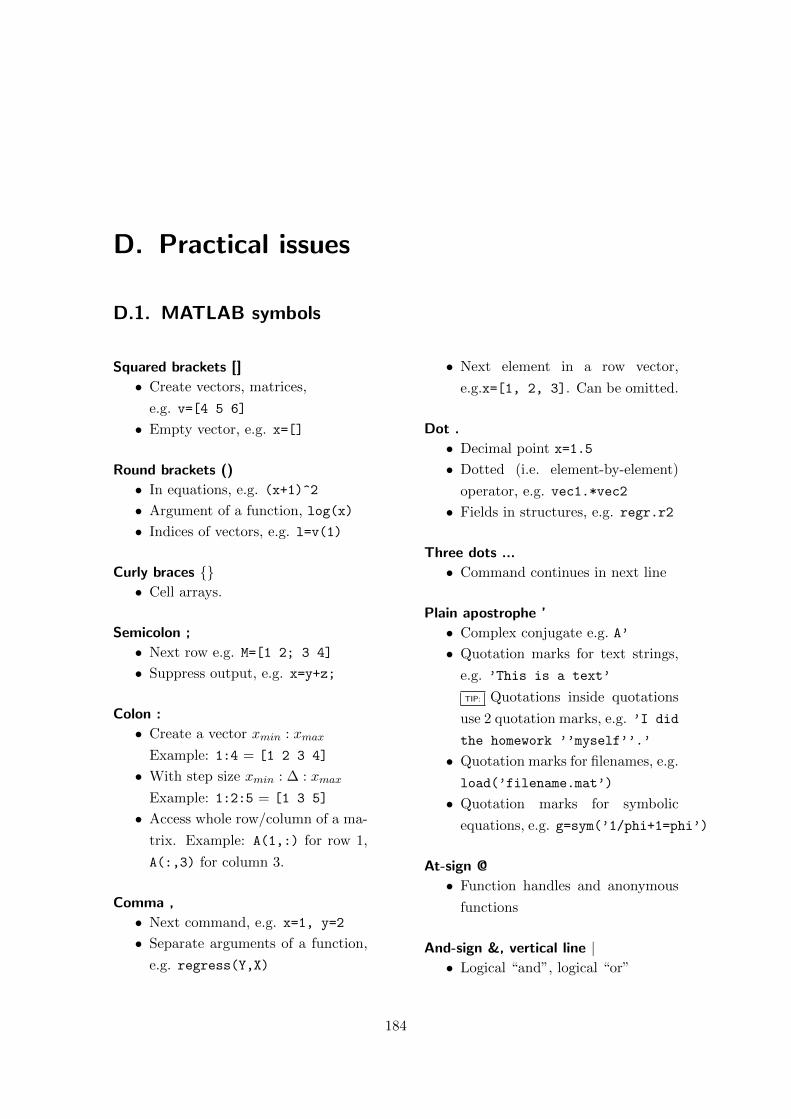
D. Practical issues
D.1. MATLAB symbols
Squared brackets []
• Create vectors, matrices,
e.g. v=[4 5 6]
• Empty vector, e.g. x=[]
Round brackets ()
• In equations, e.g. (x+1)^2
• Argument of a function, log(x)
• Indices of vectors, e.g. l=v(1)
Curly braces {}• Cell arrays.
Semicolon ;
• Next row e.g. M=[1 2; 3 4]
• Suppress output, e.g. x=y+z;
Colon :
• Create a vector xmin : xmax
Example: 1:4 = [1 2 3 4]
• With step size xmin : ∆ : xmax
Example: 1:2:5 = [1 3 5]
• Access whole row/column of a ma-
trix. Example: A(1,:) for row 1,
A(:,3) for column 3.
Comma ,
• Next command, e.g. x=1, y=2
• Separate arguments of a function,
e.g. regress(Y,X)
• Next element in a row vector,
e.g.x=[1, 2, 3]. Can be omitted.
Dot .
• Decimal point x=1.5
• Dotted (i.e. element-by-element)
operator, e.g. vec1.*vec2
• Fields in structures, e.g. regr.r2
Three dots ...
• Command continues in next line
Plain apostrophe ’
• Complex conjugate e.g. A’
• Quotation marks for text strings,
e.g. ’This is a text’
TIP: Quotations inside quotations
use 2 quotation marks, e.g. ’I did
the homework ’’myself’’.’
• Quotation marks for filenames, e.g.
load(’filename.mat’)
• Quotation marks for symbolic
equations, e.g. g=sym(’1/phi+1=phi’)
At-sign @
• Function handles and anonymous
functions
And-sign &, vertical line |• Logical “and”, logical “or”
184

D. Practical issues
D.2. MATLAB graphics
Use the plot symbol ( ) in the workspace to create a plot from data. To change a plot,
enter plottools in the command window or click on the symbol in the plot window.
A few very useful commands for plots
subplot(n,m,i) Produce n rows × m columns of plots in one figure. This
plot will be number i, counted from top left to bottom right.
hold on Overlay two plots. To start a from scratch, use hold off
axis(xmin,xmax,ymin,ymax) Rescale a plot.
A simple plot
a=randn(100,1); b=randn(100,1); Create two data series.a=cumsum(a); b=cumsum(b); A simple brownian motion.plot(a) For one plot, we don’t need x-values.plot(a,b) Plot a against b (did we want this?)n=length(a) Obtain number of data points.plot(1:n,a,’k-’,1:n,b,’r-.’) Two curves in one plot. ’k-’ stands for
“black, solid line” and ’r-.’ for “red, dash-dotted”. See help plot for more settings.
legend(’Stock01’,’Stock02’) Add legend in same order as data.
Time series
Imagine the above data are monthly observations for the years 2000 to 2007 (i.e. from the
beginning of 2000 to the beginning of 2008).To get a plot with nice labels on the x-axis,
use datetick. Assume a, b, n are still in the workspace.
t=linspace(2000,2008,100) Get the fractional year for each of the 100observations.
x=datenum(t,1,1); Convert the fractional year to date number.plot(x,a,’b-’,x,b,’r-.’) Plot with date numbers; x-axis looks strange.datetick(’x’,’mmmyy’) Get correct x-ticks.datetick(’x’,’QQ-YY’) Alternative formatting.
185

D. Practical issues
Compare values
x=1:10; Create x-valuesy_hat=2*x-2; Create estimated y-valuesy=2*x-2+randn(1,10); Create observed y-valuesplot(x,y,’+’,x,y_hat,’o’) Compare both: estimation is a circle (’o’),
observation is a cross (’+’).legend(’Observed’,’Estimated’) Add legend in same order as data.
3D plotting plus interpolation: the implied volatility surface
The problem when plotting the implied volatility surface is the fact that the data is
not regular: for short maturities, there are usually more strikes available than for long
maturities. To overcome this problem, we interpolate the data.
load iv.txt Load SP500 IV data for Jan 2, 2000
strike=iv(:,2); Data format: strike, ...
mat=iv(:,1); maturity, ...
impvol=iv(:,3); implied volatility
plot(mat,strike,’o’) The data is not evenly spaced.
Mmesh = min(mat):0.02:max(mat); Make an x-mesh ...
Smesh = min(strike):10:max(strike); and a y-mesh for interpolation.
[XI, YI] = meshgrid(Mmesh, Smesh); Produce a MATLAB meshgrid.
ZI = griddata(mat,strike,impvol,XI,YI); Perform the interpolation.
mesh(XI,YI,ZI); Produce a 3D-plot.
hold on Print the next plot over this one.
plot3(mat, strike, impvol,’o’); Plot the actual data points.
set(gca,’YDir’,’reverse’); Change strike axis for more natural view.
view([-74.5 34]); Move to a nicer viewpoint.
This code produces the following plot:
186

D. Practical issues
0
0.2
0.4
0.6
0.8
1
100012001400160018002000
0.16
0.18
0.2
0.22
0.24
Student Version of MATLAB
187

D. Practical issues
Quantiles of a distribution of sample paths
The following plot is inspired by the inflation report of the Bank of England,1 which
publishes not only the median inflation forecast, but also its quantiles.
N=200; T=20 Setup: N sample paths; T time periodsr=randn(T,N)*0.1; Simulate some log-returns ...p=exp(cumsum(r)); ... and obtain some prices.pqua=quantile(p.’,.1:.1:.9); Deciles of price distribution at every t.for q=1:4 Loop over deciles 1-4mycol=(1-q/8)*[1 1 1]; Define greys as RGB values.fill([1:T T:-1:1],[pqua(q,:) pqua(10-q,T:-1:1)],mycol,’EdgeColor’,’none’);
hold on Previous line plots grey area for 1st-9th decile,end then 2nd-8th and so onplot(1:20,pqua(5,:),’k’) Add median (5th decile) as black line
This code produces the following plot:
0 2 4 6 8 10 12 14 16 18 200.5
1
1.5
2
Function-driven plots
myfunction=@(x)0.1*x.^3-x.^2+x; Dotted operators: vector-compatible functionfplot(myfunction,[-5 10])
Saving and exporting a plot
You can use File/Save As ... in the window of the plot and select the appropriate file
format to save your plots. MATLAB sometimes crops figures, so immediately check your
output. It is much better to include the following lines of code to export your figures:
h=figure(’Visible’,’off’,’PaperUnits’,’centimeters’,’PaperSize’,[20 15],...
’PaperPositionMode’,’manual’,’PaperPosition’,[0 0 20 15]);
Add your plot commands here.
saveas(h,filemame,format);
1See http://www.bankofengland.co.uk/publications/Pages/inflationreport/.
188

D. Practical issues
The first line creates a new (empty) plot. Visible off tells MATLAB not to show
it on the screen, PaperSize is the width and and height in centimeters, the remaining
commands fix the position of the graph in the center. Finally, filename is a variable that
contains your file name and format is one of the following formats: eps, pdf, jpg, png.
Annotating plots
To annotate plots with LaTeX commands, set LaTeX as string interpreter. This works
with title, legend, xlabel, ylabel. Example:
title(’$\sqrt{x}$’,’Interpreter’,’latex’)
Changing a plot
Use the command plottools or click on the symbol in the figure window/toolstrip to
change the design of a plot. You can turn on/off individual data sets, move the location
of the caption, change colours and line styles and do many more things.
D.3. MATLAB table output
There is no command for table output in MATLAB. An improvised way to produce tables
is to create a matrix by horizontal concatenation.
FirstCol=(0.1:0.1:1).’ Create some data ...SecondCol=(100:100:1000).’
disp([FirstCol SecondCol]); Improvised table.format bank Better scaling of numbers ...disp([FirstCol SecondCol]); Better table.
For better tables use sprintf(fomatting string, variables). For details how to
define the formatting string, use doc sprintf.
sprintf(’%5.2f | %d \n’,[FirstCol SecondCol]’)
TIP: For really nice tables with many options, install the datatable package.
D.4. From MATLAB to LATEX– creating a research workflow
A large MATLAB project may easily contain hundreds of files which have different uses.
They also have different scopes: some may be of very general use, some may be only useful
189

D. Practical issues
for one special case. Like adopting naming convention, it has proved very useful to adhere
to a location convention, i.e. to organize files in different places to avoid confusion. The
guiding principle should be to avoid multiple copies of one file. These are a special source
of errors, as it will sooner or later happen that one of the copies is changed (e.g. to correct
an error), while the other ones are not.
One possible way to organize your files is the following:
Project directory
It is obvious that when starting a project, you want to put everything in one place – the
project directory. This is the place, where project-specific code should rest. However,
there are three exceptions, as described in the following:
Your personal toolbox
MATLAB scripts can only “see” files that are in the same folder or on the MATLAB path
(more below). It is a common mistake to therefore copy functions of general use into each
project folder. Every function that is used more than once should be stored in a central
place to ensure consistency. These can be
• Open source toolboxes downloaded from the web
• User-defined functions that are of general use
Create a folder called MATLABtoolbox that is located in a convenient place. Using the
command File/Set Path ... adds this folder to the list of places where MATLAB looks
for functions/m-files. Now you can conveniently call your standard functions from every
script and you have a well-organized personal library.
Note: you may want to organize your personal library in sub-folders, like for example
MATLABtoolbox/Econometrics or MATLABtoolbox/Options. If you do so, use Add With
Subfolders ... in the Set Path dialogue. Nevertheless, if you decide to create a subfolder
later, you have to add it manually using File/Set Path ....
In any case, only tested and documented functions should make it into your toolbox.
If you work a lot with MATLAB, you may want to setup a MATLABtoolboxDev as well,
where you store the not fully-tested versions. If you do so, take care that MATLABtoolbox
is on the MATLAB path before MATLABtoolboxDev to ensure that MATLAB searches first
in the toolbox and then in the developer folder.
Data directory
Following the same logic as for the personal toolbox, it is also a good idea to put all
data into a folder and add it to the MATLAB path. These two tips make it possible
190

D. Practical issues
to create different versions of a program by simply duplicating its folder, while avoiding
inconsistencies in library functions or the data set.
Work with run files
A run file is a small MATLAB program that contains only initialization code (mostly
loading a specific data set and choosing model parameters) and the calls the main program.
When working on a research project, you will probably want to test different versions
of your model with different input parameters and possibly different data sets. Simply
changing the parameters in the code is not a good idea: you might loose this information
and get stuck with perfect results that “only” lack the data generating process. An
alternative is to duplicate the whole project folder before changing the parameters. This
ensures that nothing is lost, but may lead to inconsistencies as you change code. Best is to
put all code in a directory and add this to the MATLAB path (like the personal library).
Then create one folder per run containing the run file and all results.
It is also a good idea to save important parameters with the data, just in case it gets
separated from its run file. This can be easily done by employing MATLAB structures:
A MATLAB structure for saving data with envelope informationmystruct.param=theta Saving the model parameters.mystruct.date=daterange ... range of dates of the time series (if applicable)mystruct.model=modelname Information about the detailed model specification.mystruct.results=results Finally the results.save results.mat mystruct Save the whole structure.
D.5. Practitioner’s tips
Use private functions to distribute code
A MATLAB project will easily consist of one main program and several functions. Dis-
tributing or printing such a number of files can become cumbersome, especially if the
recipient should only run the code and will not participate in the development. In this
case, private functions can provide an interesting solution. Rewrite the main program as
function without arguments and add all further functions to the file.
191

D. Practical issues
circle_mc.mFind the area of the unit circle by Monte Carlo SimulationMatLab course 2007(c) Peter GruberInspired by I. Sobol "A primer for the MC method"
Nsim = 10000;
x = 2*rand (Nsim, 2)-1; % 2D random variables between -1 and 1r2 = x(:,1).*x(:,1) + x(:,2).*x(:,2); % squared radiusx = x(r2 < 1,:); % We only take the coordinates for which r < 1
plot (x(:,1),x(:,2),'k.'); % Show the circleaxis square;
area = 4 * size(x,1) / Nsim % Calculate the area: A = r^2 * pi = pi
area =
3.1320
Published with MATLAB® 7.4
Figure D.1.: Output from Publish To HTML of circle mc.m
function mainprogram No input and output arguments< the main program > Just copy the main program. No changes required.
end % of funciton The function mainprogram ends with an end
%% ===== private functions =====
function result=myf1(arg) copy here all functions from their filesend % of funciton End all functions with an end
Use cells and code folding
Cells are very useful for structuring code. Start a cell with a double percentage sign and
give it a meaningful title. If applicable, add one or two lines of comment. To hide cells
that are not important to your work (e.g. data loading), you have to turn on code folding.
Go to File/Preferences and select Editor/Code folding. Check the box next to Cells. Now
you get a small box with a minus sign left of each cell. Click once to fold the cell, click
again to unfold it.
Publish to HTML
To produce some nice output, select File/Publish To HTML. This will run the main pro-
gram and produce a nice HTML file that is organized section-by-section and contains all
comments, the program code and the output. A fast way to produce documentation for a
program is to print the HTML document to a pdf file, see Fig. D.1.
192

D. Practical issues
Working with a remote system
If numerical tasks are very complex, one may want to execute them on a central system
instead of blocking one’s personal computer for an extended amount of time. A few things
have proved useful when working with a remote system
• Regularly save intermediate results. If the system crashes, you don’t have to start
from scratch.
• If you use solutions such as www.dropbox.com, you can synchronize the program
folders on your PC and on the remote system. Also synchronize the file in which the
intermediate results are saved. This allows for an easy check whether the system is
still running.
• Email results to yourself directly from MATLAB using the sendmail() command.
Numerical results must be converted to strings first. You can even send attach-
ments, for example graphs that you have saved to the hard drive. You have to set
MATLAB’s internet preferences to be able to use sendmail().
• MATLAB can also send and retrieve larger files via its built-in ftp() command.
Use mget() do retrieve files and mput() to send files.
193

D. Practical issues
D.6. An introduction to the Symbolic Mathematics Toolbox
Getting started
sqrt(2) Numerical solution ...
sqrt(sym(2)) This is now left as a symbol.
double(ans) Convert to a numerical result.
sym(1)/sym(3)+sym(1)/sym(6)
Symbolic variables
syms a x Define a and x as a symbolic variable for later use.
g=sym(’(x+a)/(x-a)’) A simple expression.
simplify(g) One of the most useful commands.
g=sym(’1/phi+1=phi’) The equation of the golden ratio ...
solve(g,’phi’) Tell MATLAB to solve with respect to which variable
double(ans) Get numerical values, if you like.
Substituting for variables
f=x^2+2*x+2
subs(f,x,a/2) Substitutes x with a2 .
Isolating variables
g=(’Y=c*Y+G+I-b*i-m*Y+x1*Yw’) The IS curve. Notice we left out the sym.
solve(g,’Y’) We get a neat result for Y = . . . and the multiplicator.
solve(g,’i’) Error message, because i is reserved for imaginary numbers.
syms i Declare i as a symbol.
solve(g,’i’) Now it works.
Systems of equations
f=(’M=h*Y-h/b*i’) The LM-curve
S=solve(f,g,’Y,i’) We solve the IS-LM model for Y and i
S.Y The result is a structure. We first look at the solution for Y
S.i ... and then for i.
194

D. Practical issues
Differentiate
g=(’A*K^alpha*L^(1-alpha)’) A Cobb-Douglas production function
diff(g,’L’) Differentiate with respect to L.
simplify(ans) Simplify the result, which is stored in ans.
Taylor series
f=exp(x) A symbolic function
taylor(f,3) The Taylor series up to order 2.
taylor(f,5) A longer Taylor polynomial.
taylor(f,3,0.5) Develop the polynomial around x0 = 0.5.
Integrals
f=exp(x) A symbolic function
int(f) Indefinite integral.
int(f,x,0,1) Definite integral between zero and one.
format long We want to compare this to numerical integration.
double(ans) Convert to number.
g=@(y)exp(y) Define a numerical function.
quad(g,0,1) Compare the result to the numerical integration.
Matrix Computations
syms t We create a simple matrix:
G=[cos(t) sin(t); -sin(t) cos(t)]
A=G*G We square it.
simplify(A) Nice result.
diff(A)
195

E. MATLAB @ UNI
E.1. Guide to the exercises
• The program must give correct results.
• Programs must not crash, even if the input makes no sense.
• The rules for good programming style must be observed, especially
– Clearly indicate the main program.
– Programs must have sensible documentation, including a header with all rele-vant information. The program should be readable.
– Name your program/functions as specified in the problem description. All othernames (e.g. of variables) must be self-explanatory.
– The program should be efficient.
– The solution should be a general one.
– Use foreign code (i.e. found on the web) only if allowed and then reference itcorrectly.
• Unless explicitly stated, decide yourself whether to write a function or a program.
• Test your program before handing it in and document your tests in the code header.
• Choose economically sensible values for the variables that are not specified in theproblem definition.
• Programming projects based on Octave/Freemat are accepted. Please make a com-ment referring to Octave/Freemat at the begin of the main program.
• Do not use special toolbox functions. If not stated otherwise, only the statistics andoptimization toolboxes are allowed.1
Bonus for admitting code that does not work
Understanding what does not work is a first step to solving the problem. If you notice that
some part of your solution does not work as required, make a short(!) comment explaining
1If your are not sure if a function is part of a certain toolbox, type doc functionname in MATLAB, whichwill open a help browser. In the top of the browser, you see a hierarchy of keywords. If this hierarchystarts with MATLAB, the function is a MATLAB core function. If it starts with (Some Name) Toolbox,it is part of a toolbox.
196

E. MATLAB @ UNI
what does not work. You will get fewer points deducted than when simply handing in a
program that does not work.
Hand in interactive exercises using a diary
You can use MATLAB’s “logbook” command for interactive problem sets.
diary (’filename’) Specify file name and start diary.Find the file in the current directory as explained in Fig. 2.1.
%<Your text answer> Answer text questions as MATLAB comment.Start each line with %
diary off Suspend (temporarily) the diary, e.g. for experimenting.diary on Start the diary again after suspension.diary off Turn the diary off at the end to close the file.
E.2. Obtaining and installing MATLAB and its open-source
alternatives
The MATLAB student license is available online and at the university bookshop for a
price of ca. CHF 100. The license includes the Symbolic Mathematics Toolbox, the Statis-
tics Toolbox and the Optimization Toolbox (and a few engineering-related toolboxes).
Octave is a program under the GNU public license that can interpret MATLAB com-
mands. It is included in many Linux distributions. Octave is like a MATLAB that contains
only a command window and requires and external editor. Free text editors with syntax
highlighting are Notepad++ editor for MS Windows and TextWrangler for Mac OS X.
The programs are available at:
• www.octave.org
• www.notepad-plus-plus.org
• www.barebones.com/products/textwrangler, you need to install the MATLAB
language module from www.esm.psu.edu/~ajm138/matlab_utils
Unfortunately, Octave is only 95% compatible to MATLAB. In many cases, minor
changes are necessary to run a MATLAB program under Octave.
Currently, Octave/Freemat are not actively supported in the course (i.e. demo programs
are not checked for compatibility). Students may use Octave/Freemat at their own risk.
Freemat is yet another alternative to MATLAB, which is slightly easier to use, as it has
its own editor. It is available at freemat.sourceforge.net. For the pros and cons of
Octave, MATLAB and FreeMat, see the table below.
197

E. MATLAB @ UNI
Julia is a recent and very fast, very powerful programming language that is similar to
MATLAB. Julia is free software and available at www.julialang.org
MATLAB Octave Freemat
Commercial product Free (GPL) Free
User-friendly (editor ...) Calculations only Interface similar to MATLAB
– 95% compatible to MATLAB > 95% compatibility
MathWorks toolboxes Public collections of code Public collections of code
Help function (text),
online documentation,
printed documentation
Help function (text), wiki, can
use some MATLAB documen-
tation
Help function (text), online
documentation, can use some
MATLAB documentation
Activation process Part of Linux distributions Download, use and share
CHF 2000+ (student: 100) CHF 0 plus your time CHF 0 plus your time
MATLAB @ HSG in PC lab 01-U102 features 25 licenses of MATLAB and the follow-
ing toolboxes: Symbolic Mathematics, Statistics, Optimization, Financial and Financial
Derivatives as well as James P. LeSage’s Econometrics Toolbox. MATLAB is only available
there and can be used freely by students. Check if the lab is not booked.
MATLAB @ UNIGE You can buy MATLAB for classroom and personal use at http:
//www.mathworks.ch/academia/student_version/
198

Bibliography
Abadir, Karim M., and Jan R. Magnus (2005) Matrix Algebra (Econometric Exercises)(Cambrindge University Press)
Brandimarte, Paolo (2006) Numerical Methods in Finance and Economics (Wiley andSons)
Carr, P., and D. Madan (1999) ‘Option valuation using the fast fourier transform.’ Journalof Computational Finance 2, 61–73
Chong, Edwin K.P., and Stanilaw H. Zak (2008) An introduction to Optimization (Wiley)
Christoffersen, Peter, Steve Heston, and Kris Jacobs (2009) ‘The shape and term structureof the index option smirk: Why multifactor stochastic volatility models work so well.’Management Science 55, 1914–1932
Creel, Michael (2006) Econometrics (Online, http://pareto.uab.es/mcreel/
Econometrics/)
Fang, Fang, and Kees Oosterlee (2008) ‘A novel pricing method for european options basedon fourier-cosine expansions.’ SIAM Journal on Scientific Computing 31(2), 826–848
Gentle, James E. (2007) Matrix Algebra (Springer)
Gilli, Manfred, Dietmar Maringer, and Enrico Schumann (2011) Numerical Methods andOptimization in Finance (Academic Press, New York.)
Glasserman, Paul (2003) Monte Carlo Methods in Financial Engineering (Springer)
Greene, W. H. (2002) Econometric Analysis (Prentice Hall; 5th edition)
Gut, Allan (2005) Probability: A Graduate Course (Springer)
Hanselman, D., and B. Littlefield (2005) Mastering Matlab 7 (Pearson Education Interna-tional)
Hardle, W., and L. Simar (2003) Applied Multivariate Statistics (Springer)
Judd, Kenneth L. (1998) Numerical Methods in Economics (MIT Press)
Kerrighan, Brian W., and P. J. Plauger (1974) The elements of programming style(McGraw-Hill)
Kharab, A., and R. B. Guenther (2006) Introduction to numerical methods – A MATLABapproach (Chapman & Hall)

Kuniciky, David C. (2004) Matlab Programming (Pearson Prentice Hall)
LeSage, James P. (1999) Applied Econometrics using MATLAB (Online, www.
spatial-econometrics.com)
Lord, Roger, and Christian Kahl (2008) ‘Complex logarithms in heston-like models.’ Work-ing paper February 21st, 2008
Mathews, John D., and Kurtis D. Fink (2004) Numerical Methods using Matlab (Pear-son Education, also available at http://math.fullerton.edu/mathews/n2003/
NumericalUndergradMod.html)
Metropolis, M., and S. Ulam (1949) ‘The monte carlo method.’ Journal of the AmericanStatistical Association 49, 335–341
Moler, Cleve (2004) Numerical Computing with Matlab (SIAM (also available at http:
//www.mathworks.com/moler/))
Moore, Gordon E. (1965) ‘Cramming more components onto integrated circuits.’ Electron-ics Magazine
Opfer, Gerhard (2004) Numerische Mathematik fur Anfanger (Vieweg)
Pedersen, M. S., and K. B. Petersen (2007) The Matrix Cookbook (http://matrixcookbook.com/)
Simon, C. P., and L. Blume (1994) Mathematics for economists (Norton)
Stanoyevitch, Alexander (2005) Introduction to MATLAB with Numerical Preliminaries(Wile)
Verbeek, M. (2004) Modern Econometrics (Wiley)
Wooldridge, J. (2005) Introductory Econometrics: A Modern Approach (South-WesternCollege Pub; 3 edition)

Final remark:
Writing a program is
half science and half handicraft,
so both is useful:
thinking and training.