SciPy: Scientific Computing

Hendrik Speleers

Lab Calc2019-2020

SciPy: Scientific Computing

● Overview– Collection of SciPy toolboxes

● E.g., special functions, input and output

– Interpolation● Spline interpolation and smoothing

– Optimization● Local and global optimization

– Integration

– Linear algebra● Solving linear systems + eigenvalue problems

Lab Calc2019-2020

SciPy: Scientific Computing

● SciPy– Scientific Python

– Collection of toolboxes● Dedicated to common issues in scientific computing● Examples: interpolation, optimization, linear algebra, image processing, ...● Scipy’s routines are optimized and tested● Similar to: Matlab’s toolboxes, GSL (GNU Scientific Library for C++)

Lab Calc2019-2020

SciPy: Scientific Computing

● SciPy scipy.cluster vector quantization / kmeans

scipy.constants physical and mathematical constants

scipy.fftpack Fourier transform

scipy.integrate integration

scipy.interpolate interpolation

scipy.io data input and output

scipy.linalg linear algebra

scipy.ndimage n-dimensional images

scipy.odr orthogonal distance regression

scipy.optimize optimization

scipy.signal signal processing

scipy.sparse sparse matrices

scipy.spatial spatial data structures and algorithms

scipy.special special mathematical functions

scipy.stats statistics

Lab Calc2019-2020

SciPy: Scientific Computing

● Special functions

– Module special

– Examples● Bessel functions: special.jn(v, z)

● Elliptic functions: special.ellipj(u, m)

● Gamma function: special.gamma(z)

● Error function: special.erf(z)

– Functions operate elementwise on whole arrays

from scipy import special

Lab Calc2019-2020

SciPy: Scientific Computing

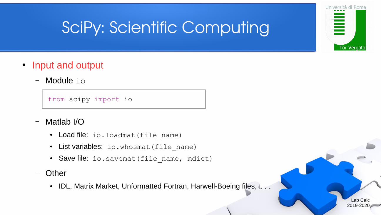
● Input and output

– Module io

– Matlab I/O● Load file: io.loadmat(file_name)

● List variables: io.whosmat(file_name)

● Save file: io.savemat(file_name, mdict)

– Other● IDL, Matrix Market, Unformatted Fortran, Harwell-Boeing files, ...

from scipy import io

Lab Calc2019-2020

SciPy: Scientific Computing

● Input and output– Example

In [1]: a = np.ones((3, 2))

In [2]: io.savemat('file.mat', {'a': a})

In [3]: io.whosmat('file.mat')

Out[3]: [('a', (3, 2), 'double')]

In [4]: data = io.loadmat('file.mat')

In [5]: data['a']

Out[5]: array([[1., 1.], ...: [1., 1.], ...: [1., 1.]])

Lab Calc2019-2020

SciPy: Scientific Computing

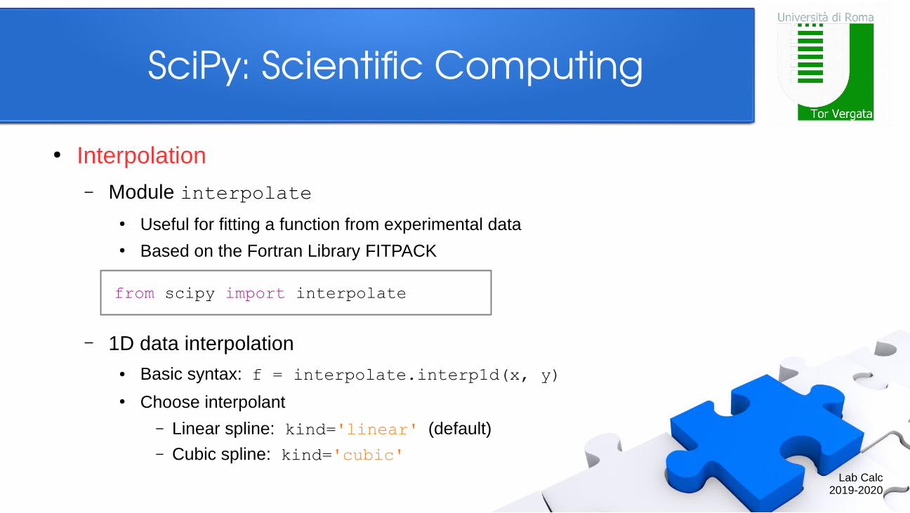
● Interpolation

– Module interpolate● Useful for fitting a function from experimental data● Based on the Fortran Library FITPACK

– 1D data interpolation● Basic syntax: f = interpolate.interp1d(x, y)● Choose interpolant

– Linear spline: kind='linear' (default)– Cubic spline: kind='cubic'

from scipy import interpolate

Lab Calc2019-2020

SciPy: Scientific Computing

● Interpolation– Example

In [1]: x = np.linspace(0.0, 4.0, 5) ...: y = np.cos(x**2 / 3.0 + 4.0)

In [2]: f1 = interpolate.interp1d(x, y)

In [3]: f2 = interpolate.interp1d(x, y, ...: kind='cubic')

In [4]: t = np.linspace(0.0, 4.0, 50) ...: plt.plot(x, y, 'o') ...: plt.plot(t, f1(t), '-') ...: plt.plot(t, f2(t), '--') ...: plt.legend(('data', 'linear', 'cubic'))

Lab Calc2019-2020

SciPy: Scientific Computing

● Interpolation– 1D spline smoothing

● Spline representation – tck = interpolate.splrep(x, y, w=None, k=3, s=None, t=None)– Input: data points (x, y), weights w, degree k, smoothing factor s, knots t– Output: tck = (t, c, k) collects knots t, coefficients c, degree k

● Spline evaluation – y = interpolate.splev(x, tck, der=0)– Input: points x, spline data tck, order of derivative der– Output: spline values y

● Other: interpolate.splint, interpolate.sproot, ...

Lab Calc2019-2020

SciPy: Scientific Computing

● Interpolation– Example

In [1]: x = np.linspace(-3.0, 3.0, 50) ...: r = 0.05 * np.random.randn(50) ...: y = np.exp(-x**2) + r

In [2]: tck = interpolate.splrep(x, y, ...: s=0.2)

In [3]: t = np.linspace(-3.0, 3.0, 100) ...: spl = interpolate.splev(t, tck)

In [4]: plt.plot(x, y, 'o') ...: plt.plot(t, spl, '-') ...: plt.legend(('data', 'spline'))

Lab Calc2019-2020

SciPy: Scientific Computing

● Optimization

– Module optimize

– 1D optimization● Basic syntax: res = optimize.minimize_scalar(fun, bounds=None)● Choose method

– Brent method: method='Brent' (default)– Golden section: method='Golden'– Bounded Brent: method='Bounded'

from scipy import optimize

Lab Calc2019-2020

SciPy: Scientific Computing

● Optimization– Local optimization

● res = optimize.minimize(fun, x0, jac=None, hess=None, bounds=None)● Choose method

– Quasi-Newton method: method='BFGS' (default)– Conjugate gradients: method='CG', 'Newton-CG'– Trust-region methods: method='trust-ncg', 'trust-krylov', 'trust-exact'– ...

– Global optimization● res = optimize.basinhopping(fun, x0)

● Based on local method: minimizer_kwargs={'method':'BFGS'}

Lab Calc2019-2020

SciPy: Scientific Computing

● Optimization– Linear programming

● minx cTx

s.t. Aubx ≤ b

ub, A

eqx = b

eq, l ≤ x ≤ u

● res = optimize.linprog(c, A_ub=None, b_ub=None, A_eq=None, b_eq=None, bounds=None)

● Choose method

– Quasi-Newton method: method='interior-point' (default)– Simplex method: method='revised simplex', 'simplex'

– Other● Root finding: optimize.root_scalar, optimize.root

Lab Calc2019-2020

SciPy: Scientific Computing

● Optimization– Example

In [1]: def f(x): ...: return x**2 + 10.0*np.sin(x)

In [2]: rg = optimize.minimize_scalar(f)

In [3]: rg.x

Out[3]: -1.3064400120612139

In [4]: rl = optimize.minimize_scalar(f, ...: bounds=(2, 7), method='bounded')

In [5]: rl.x

Out[5]: 3.8374681582973356

Lab Calc2019-2020

SciPy: Scientific Computing

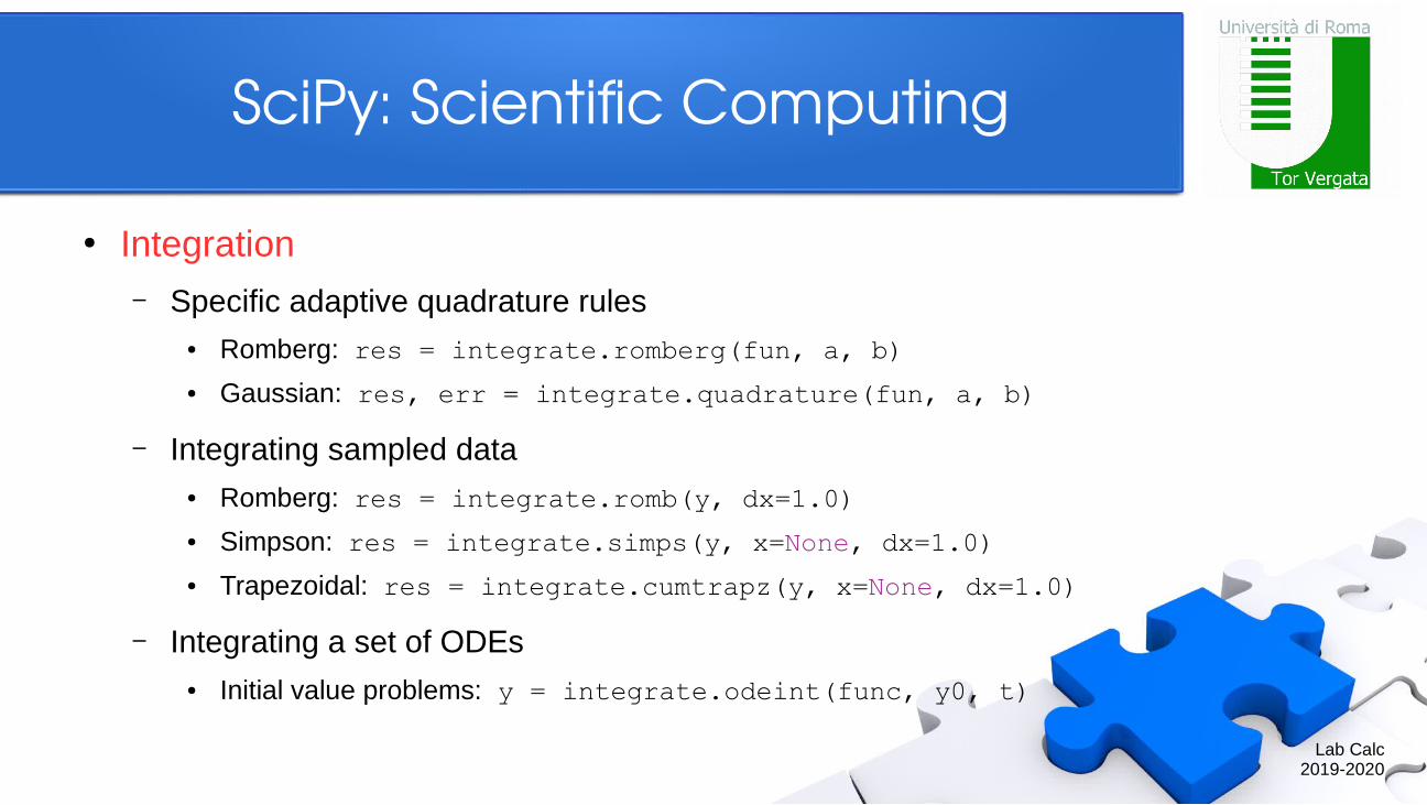
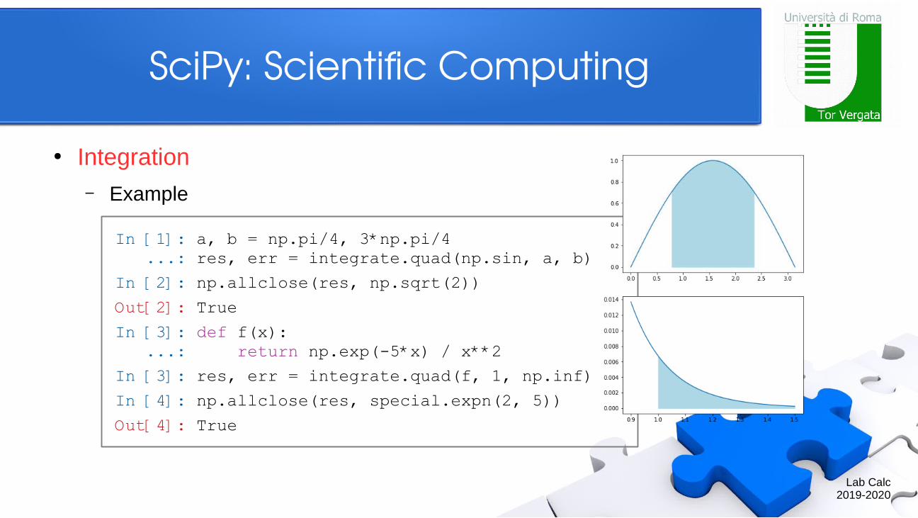
● Integration

– Module integrate● Provides several integration techniques, including an ODE integrator● Based on the Fortran Libraries QUADPACK, ODEPACK, ...

– 1D adaptive quadrature● Basic syntax: res, err = integrate.quad(fun, a, b)● Computes

from scipy import integrate

res≈∫a

b

fun(t)dt

Lab Calc2019-2020

SciPy: Scientific Computing

● Integration– Specific adaptive quadrature rules

● Romberg: res = integrate.romberg(fun, a, b)

● Gaussian: res, err = integrate.quadrature(fun, a, b)

– Integrating sampled data● Romberg: res = integrate.romb(y, dx=1.0)

● Simpson: res = integrate.simps(y, x=None, dx=1.0)

● Trapezoidal: res = integrate.cumtrapz(y, x=None, dx=1.0)

– Integrating a set of ODEs● Initial value problems: y = integrate.odeint(func, y0, t)

Lab Calc2019-2020

SciPy: Scientific Computing

● Integration– Example

In [1]: a, b = np.pi/4, 3*np.pi/4 ...: res, err = integrate.quad(np.sin, a, b)

In [2]: np.allclose(res, np.sqrt(2))

Out[2]: True

In [3]: def f(x): ...: return np.exp(-5*x) / x**2

In [3]: res, err = integrate.quad(f, 1, np.inf)

In [4]: np.allclose(res, special.expn(2, 5))

Out[4]: True

Lab Calc2019-2020

SciPy: Scientific Computing

● Linear algebra

– Module linalg● Standard linear algebra operations● Relying on efficient implementations (BLAS, LAPACK)

– Basic operations● Determinant: linalg.det(a)

● Inverse: linalg.inv(a)

● Norm: linalg.norm(a, ord=None, axis=None)

from scipy import linalg

Lab Calc2019-2020

SciPy: Scientific Computing

● Linear algebra– Matrix decompositions

● LU: p, l, u = linalg.lu(a)

● Cholesky: c = linalg.cholesky(a)

● QR: q, r = linalg.qr(a)

● SVD: u, s, v = linalg.svd(a)

● Schur: t, z = linalg.schur(a)

– Special matrices● Block diagonal: linalg.block_diag(*arrs)

● Toeplitz: linalg.toeplitz(c, r=None)

● Hankel: linalg.hankel(c, r=None)

Lab Calc2019-2020

SciPy: Scientific Computing

● Linear algebra– Solve linear system a * x = b

● Basic syntax: x = linalg.solve(a, b)● Choose solver by specifying type

– Generic: assume_a='gen' (default) → LAPACK solver ?GESV– Symmetric: assume_a='sym' → LAPACK solver ?SYSV– Hermitian: assume_a='her' → LAPACK solver ?HESV– Positive definite: assume_a='pos' → LAPACK solver ?POSV

– Other solvers● Banded: x = linalg.solve_banded((l, u), ab, b)

● Triangular: x = linalg.solve_triangular(a, b, lower=False)

Lab Calc2019-2020

SciPy: Scientific Computing

● Linear algebra– Eigenvalue problem a * v = w * b * v

● Eigenvalues: w = linalg.eigvals(a, b=None)

● Eigenvectors: w, v = linalg.eig(a, b=None)

– Symmetric eigenvalue problem● Symmetric: w, v = eigh(a, b=None)

● Symmetric banded: w, v = linalg.eig_banded(a_band, lower=False)

– Singular value problem● Singular values: s = linalg.svdvals(a)

● SVD: u, s, v = linalg.svd(a)

Lab Calc2019-2020

SciPy: Scientific Computing

● Linear algebra– Example

In [1]: a = np.array([[1, 2], [3, 4]]) ...: b = np.array([[5], [6]])

In [2]: linalg.inv(a).dot(b) # slow

Out[2]: array([[-4. ], ...: [ 4.5]])

In [3]: np.linalg.solve(a, b) # fast

Out[3]: array([[-4. ], ...: [ 4.5]])

In [4]: np.linalg.det(a)

Out[4]: -2.0000000000000004

Avoid inverting

a matrix unless

strictly needed!