scilab textbook companion for chemical engineering

Scilab Textbook Companion forChemical Engineering Thermodynamics

by P. Ahuja1

Created byShashwatB.Tech

Chemical EngineeringIIT BHU Varanasi

College TeacherPrakash KotechaCross-Checked by

May 23, 2016

1Funded by a grant from the National Mission on Education through ICT,http://spoken-tutorial.org/NMEICT-Intro. This Textbook Companion and Scilabcodes written in it can be downloaded from the ”Textbook Companion Project”section at the website http://scilab.in

Book Description

Title: Chemical Engineering Thermodynamics

Author: P. Ahuja

Publisher: PHI Learning Private Limited, New Delhi

Edition: 1

Year: 2009

ISBN: 9788120336377

1

Scilab numbering policy used in this document and the relation to theabove book.

Exa Example (Solved example)

Eqn Equation (Particular equation of the above book)

AP Appendix to Example(Scilab Code that is an Appednix to a particularExample of the above book)

For example, Exa 3.51 means solved example 3.51 of this book. Sec 2.3 meansa scilab code whose theory is explained in Section 2.3 of the book.

2

Contents

List of Scilab Codes 4

1 Introduction 5

2 Equations of state 21

3 The First Law and Its Applications 51

4 The Secomd Law and Its Applications 89

5 Exergy 127

6 Chemical reactions 148

7 Thermodynamic property relations of pure substance 170

8 Thermodynamic Cycles 214

10 Residual Properties by Equations of State 233

11 Properties of a Component in a Mixture 302

12 Partial Molar Volume and Enthalpy from Experimental Data 314

13 Fugacity of a Component in a Mixture by Equations ofState 328

14 Activity Coefficients Models for Liquid Mixtures 340

15 Vapour Liquid Equilibria 365

3

16 Other Phase Equilibria 415

17 Chemical Reactions Equilibria 434

18 Adiabatic Reaction Temperature 488

4

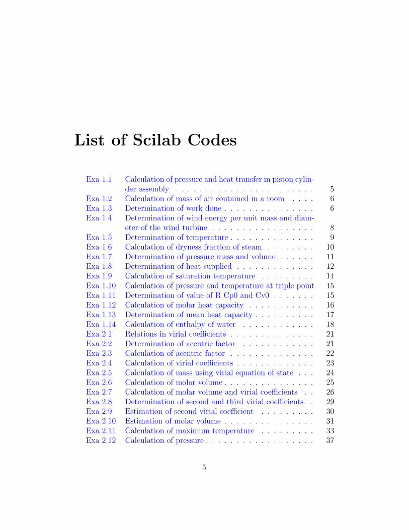
List of Scilab Codes

Exa 1.1 Calculation of pressure and heat transfer in piston cylin-der assembly . . . . . . . . . . . . . . . . . . . . . . . 5

Exa 1.2 Calculation of mass of air contained in a room . . . . 6Exa 1.3 Determination of work done . . . . . . . . . . . . . . . 6Exa 1.4 Determination of wind energy per unit mass and diam-

eter of the wind turbine . . . . . . . . . . . . . . . . . 8Exa 1.5 Determination of temperature . . . . . . . . . . . . . . 9Exa 1.6 Calculation of dryness fraction of steam . . . . . . . . 10Exa 1.7 Determination of pressure mass and volume . . . . . . 11Exa 1.8 Determination of heat supplied . . . . . . . . . . . . . 12Exa 1.9 Calculation of saturation temperature . . . . . . . . . 14Exa 1.10 Calculation of pressure and temperature at triple point 15Exa 1.11 Determination of value of R Cp0 and Cv0 . . . . . . . 15Exa 1.12 Calculation of molar heat capacity . . . . . . . . . . . 16Exa 1.13 Determination of mean heat capacity . . . . . . . . . . 17Exa 1.14 Calculation of enthalpy of water . . . . . . . . . . . . 18Exa 2.1 Relations in virial coefficients . . . . . . . . . . . . . . 21Exa 2.2 Determination of acentric factor . . . . . . . . . . . . 21Exa 2.3 Calculation of acentric factor . . . . . . . . . . . . . . 22Exa 2.4 Calculation of virial coefficients . . . . . . . . . . . . . 23Exa 2.5 Calculation of mass using virial equation of state . . . 24Exa 2.6 Calculation of molar volume . . . . . . . . . . . . . . . 25Exa 2.7 Calculation of molar volume and virial coefficients . . 26Exa 2.8 Determination of second and third virial coefficients . 29Exa 2.9 Estimation of second virial coefficient . . . . . . . . . 30Exa 2.10 Estimation of molar volume . . . . . . . . . . . . . . . 31Exa 2.11 Calculation of maximum temperature . . . . . . . . . 33Exa 2.12 Calculation of pressure . . . . . . . . . . . . . . . . . . 37

5

Exa 2.13 Calculation of pressure . . . . . . . . . . . . . . . . . . 38Exa 2.14 Determination of compressibility factor . . . . . . . . 40Exa 2.15 Determination of molar volume . . . . . . . . . . . . . 42Exa 2.16 Calculation of volume . . . . . . . . . . . . . . . . . . 44Exa 2.17 Estimation of compressibility factor . . . . . . . . . . 47Exa 3.1 Calculation of temperature . . . . . . . . . . . . . . . 51Exa 3.2 Calculation of heat required . . . . . . . . . . . . . . . 54Exa 3.3 Calculation of temperature internal energy and enthalpy 55Exa 3.4 Calculation of work done . . . . . . . . . . . . . . . . 57Exa 3.5 Calculation of work done . . . . . . . . . . . . . . . . 59Exa 3.6 Calculation of work done . . . . . . . . . . . . . . . . 61Exa 3.7 Proving a mathematical relation . . . . . . . . . . . . 66Exa 3.8 Calculation of work done . . . . . . . . . . . . . . . . 66Exa 3.9 Calculation of final temperature . . . . . . . . . . . . 68Exa 3.10 Finding expressions for temperature and pressure . . . 69Exa 3.11 Calculation of final pressure . . . . . . . . . . . . . . . 70Exa 3.12 Calculation of slope and work done . . . . . . . . . . . 71Exa 3.13 Calculation of work done and final temperature . . . . 73Exa 3.14 Calculation of powerand discharge head . . . . . . . . 75Exa 3.15 Calculation of discharge velocity . . . . . . . . . . . . 76Exa 3.16 Calculation of change in enthalpy . . . . . . . . . . . . 78Exa 3.17 Calculation of work done and change in enthalpy . . . 78Exa 3.18 Calculation of work done per unit mass . . . . . . . . 80Exa 3.19 Calculation of inlet and outlet velocity and power . . . 81Exa 3.20 Proving a mathematical relation . . . . . . . . . . . . 83Exa 3.21 Determination of equilibrium temperature . . . . . . . 84Exa 3.22 Determination of mass . . . . . . . . . . . . . . . . . . 86Exa 4.1 Calculation of entropy change . . . . . . . . . . . . . . 89Exa 4.2 Determination of whether the process is reversible or not 91Exa 4.3 Calculation of final pressure temperature and increase

in entropy . . . . . . . . . . . . . . . . . . . . . . . . . 93Exa 4.4 CAlculation of final temperature heat transfer and change

of entropy . . . . . . . . . . . . . . . . . . . . . . . . . 95Exa 4.5 Calculation of final temperature work and heat transfer 98Exa 4.6 Calculation of final temperature and work done . . . . 101Exa 4.7 Determination of index of isentropic expansion . . . . 102Exa 4.8 Determination of entropy production . . . . . . . . . . 104Exa 4.9 Determination of work required and exit temperature . 105

6

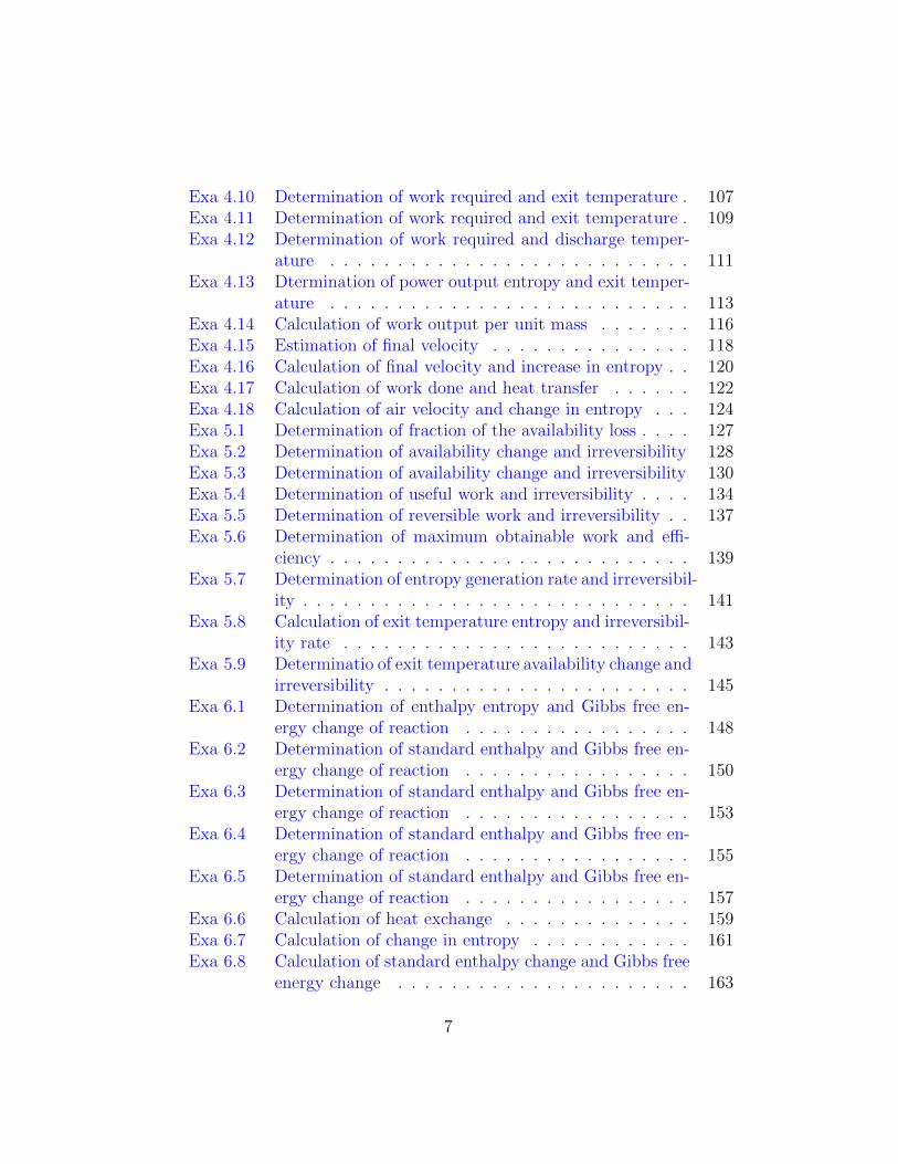
Exa 4.10 Determination of work required and exit temperature . 107Exa 4.11 Determination of work required and exit temperature . 109Exa 4.12 Determination of work required and discharge temper-

ature . . . . . . . . . . . . . . . . . . . . . . . . . . . 111Exa 4.13 Dtermination of power output entropy and exit temper-

ature . . . . . . . . . . . . . . . . . . . . . . . . . . . 113Exa 4.14 Calculation of work output per unit mass . . . . . . . 116Exa 4.15 Estimation of final velocity . . . . . . . . . . . . . . . 118Exa 4.16 Calculation of final velocity and increase in entropy . . 120Exa 4.17 Calculation of work done and heat transfer . . . . . . 122Exa 4.18 Calculation of air velocity and change in entropy . . . 124Exa 5.1 Determination of fraction of the availability loss . . . . 127Exa 5.2 Determination of availability change and irreversibility 128Exa 5.3 Determination of availability change and irreversibility 130Exa 5.4 Determination of useful work and irreversibility . . . . 134Exa 5.5 Determination of reversible work and irreversibility . . 137Exa 5.6 Determination of maximum obtainable work and effi-

ciency . . . . . . . . . . . . . . . . . . . . . . . . . . . 139Exa 5.7 Determination of entropy generation rate and irreversibil-

ity . . . . . . . . . . . . . . . . . . . . . . . . . . . . . 141Exa 5.8 Calculation of exit temperature entropy and irreversibil-

ity rate . . . . . . . . . . . . . . . . . . . . . . . . . . 143Exa 5.9 Determinatio of exit temperature availability change and

irreversibility . . . . . . . . . . . . . . . . . . . . . . . 145Exa 6.1 Determination of enthalpy entropy and Gibbs free en-

ergy change of reaction . . . . . . . . . . . . . . . . . 148Exa 6.2 Determination of standard enthalpy and Gibbs free en-




ergy change of reaction . . . . . . . . . . . . . . . . . 157Exa 6.6 Calculation of heat exchange . . . . . . . . . . . . . . 159Exa 6.7 Calculation of change in entropy . . . . . . . . . . . . 161Exa 6.8 Calculation of standard enthalpy change and Gibbs free

energy change . . . . . . . . . . . . . . . . . . . . . . 163

7

Exa 6.9 Calculation of standard enthalpy change and Gibbs freeenergy change . . . . . . . . . . . . . . . . . . . . . . 165

Exa 6.10 Determination of standard enthalpy change and Gibbsfree energy change . . . . . . . . . . . . . . . . . . . . 167

Exa 7.1 Proving a mathematical relation . . . . . . . . . . . . 170Exa 7.2 Proving a mathematical relation . . . . . . . . . . . . 171Exa 7.3 Proving a mathematical relation . . . . . . . . . . . . 171Exa 7.4 Proving a mathematical relation . . . . . . . . . . . . 172Exa 7.5 Proving a mathematical relation . . . . . . . . . . . . 172Exa 7.6 Estimation of entropy change . . . . . . . . . . . . . . 173Exa 7.7 Determination of work done . . . . . . . . . . . . . . . 174Exa 7.8 Proving a mathematical relation . . . . . . . . . . . . 175Exa 7.9 Proving a mathematical relation . . . . . . . . . . . . 176Exa 7.10 Proving a mathematical relation . . . . . . . . . . . . 177Exa 7.11 Proving a mathematical relation . . . . . . . . . . . . 177Exa 7.12 Evaluation of beta and K for nitrogen gas . . . . . . . 178Exa 7.13 Calculation of temperature change and entropy change

of water . . . . . . . . . . . . . . . . . . . . . . . . . . 179Exa 7.14 Estimation of change in entropy and enthalpy . . . . . 181Exa 7.15 Calculation of percentage change in volume . . . . . . 182Exa 7.16 Determination of enthalpy and entropy change . . . . 183Exa 7.17 Proving a mathematical relation . . . . . . . . . . . . 185Exa 7.18 Proving a mathematical relation . . . . . . . . . . . . 185Exa 7.19 Proving a mathematical relation . . . . . . . . . . . . 186Exa 7.20 Proving a mathematical relation . . . . . . . . . . . . 186Exa 7.21 Proving a mathematical relation . . . . . . . . . . . . 187Exa 7.22 Calculation of volume expansivity and isothermal com-

pressibility . . . . . . . . . . . . . . . . . . . . . . . . 188Exa 7.23 Estimation of specific heat capacity . . . . . . . . . . 189Exa 7.24 Estimation of specific heat capacity . . . . . . . . . . 190Exa 7.25 Calculation of volume expansivity and isothermal com-

pressibility . . . . . . . . . . . . . . . . . . . . . . . . 191Exa 7.26 Calculation of mean Joule Thomson coefficient . . . . 192Exa 7.27 Estimation of Joule Thomson coefficient . . . . . . . . 194Exa 7.28 Proving a mathematical relation . . . . . . . . . . . . 195Exa 7.29 Proving a mathematical relation . . . . . . . . . . . . 196Exa 7.30 Calculation of pressure . . . . . . . . . . . . . . . . . . 197Exa 7.31 Calculation of enthalpy change and entropy change . . 198

8

Exa 7.32 Estimation of ratio of temperature change and pressurechange . . . . . . . . . . . . . . . . . . . . . . . . . . 199

Exa 7.33 Determination of boiling point of water . . . . . . . . 200Exa 7.34 Calculation of enthalpy and entropy of vaporization of

water . . . . . . . . . . . . . . . . . . . . . . . . . . . 201Exa 7.35 Estimation of heat of vaporization of water . . . . . . 202Exa 7.36 Calculation of latent heat of vaporization . . . . . . . 203Exa 7.37 Determination of temperature dependence . . . . . . . 204Exa 7.38 Calculation of fugacity of water . . . . . . . . . . . . . 207Exa 7.39 Estimation of fugacity of saturated steam . . . . . . . 208Exa 7.40 Estimation of fugacity of steam . . . . . . . . . . . . . 209Exa 7.41 Determination of fugacities at two states . . . . . . . . 212Exa 8.1 Calculation of work done . . . . . . . . . . . . . . . . 214Exa 8.2 Calculation of efficiency of Rankine cycle . . . . . . . 217Exa 8.3 Calculatrion of COP of carnot refrigerator and heat re-

jected . . . . . . . . . . . . . . . . . . . . . . . . . . . 219Exa 8.4 Calculation of minimum power required . . . . . . . . 220Exa 8.5 Determination of COP and power required . . . . . . 221Exa 8.6 Determination of maximum refrigeration effect . . . . 221Exa 8.7 Determination of refrigeration effect power consumed

and COP of refrigerator . . . . . . . . . . . . . . . . . 222Exa 8.8 Calculation of amount of air . . . . . . . . . . . . . . . 225Exa 8.9 Calculation of amount of air and temperature . . . . . 227Exa 8.10 Determination of temperature of air . . . . . . . . . . 230Exa 10.1 Determination of expression for residual enthalpy inter-

nal energy and Gibbs free energy . . . . . . . . . . . . 233Exa 10.2 Preparation of fugacity and fugacity coefficient . . . . 234Exa 10.3 Calculation of enthalpy entropy and internal energy change 235Exa 10.4 Calculation of molar heat capacity . . . . . . . . . . . 238Exa 10.5 Calculation of final temperature after expansion . . . . 240Exa 10.6 Calculation of fugacity of liquid benzene . . . . . . . . 242Exa 10.7 Calculation of molar enthalpy . . . . . . . . . . . . . . 244Exa 10.8 Determination of second and third virial coefficients and

fugacity . . . . . . . . . . . . . . . . . . . . . . . . . . 245Exa 10.9 Determination of second and third virial coefficients . 248Exa 10.10 Determination of work done and the exit temperature 250Exa 10.11 Calculation of temperature and pressure . . . . . . . . 256

9

Exa 10.12 Calculation of change of internal energy enthalpy en-tropy and exergy . . . . . . . . . . . . . . . . . . . . . 260

Exa 10.13 Calculation of change in enthalpy . . . . . . . . . . . . 263Exa 10.14 Calculation of final temperature . . . . . . . . . . . . 265Exa 10.15 Proving a mathematical relation . . . . . . . . . . . . 266Exa 10.16 Proving a mathematical relation . . . . . . . . . . . . 267Exa 10.17 Determination of work done and the exit temperature 267Exa 10.18 Proving a mathematical relation . . . . . . . . . . . . 271Exa 10.19 Calculation of molar volume and fugacity . . . . . . . 271Exa 10.20 Calculation of enthalpy and entropy change . . . . . . 273Exa 10.21 Calculation of fugacity . . . . . . . . . . . . . . . . . . 276Exa 10.22 Calculation of enthalpy change . . . . . . . . . . . . . 278Exa 10.23 Calculation of fugacity of water vapour . . . . . . . . 282Exa 10.24 Determination of change in internal energy . . . . . . 284Exa 10.25 Calculation of enthalpy and entropy change . . . . . . 287Exa 10.26 Calculation of final temperature and pressure . . . . . 290Exa 10.27 Calculation of vapour pressure . . . . . . . . . . . . . 295Exa 10.28 Determination of vapour pressure . . . . . . . . . . . . 298Exa 11.1 Determination of volumes of ethanol and water . . . . 302Exa 11.2 Developing an expression . . . . . . . . . . . . . . . . 303Exa 11.3 Determination of partial molar volume . . . . . . . . . 304Exa 11.4 Calculation of enthalpies . . . . . . . . . . . . . . . . . 305Exa 11.5 Developing an expression and calculation for enthalpy

change of mixture . . . . . . . . . . . . . . . . . . . . 307Exa 11.6 Proving a mathematical relation . . . . . . . . . . . . 308Exa 11.7 Proving a mathematical relation . . . . . . . . . . . . 308Exa 11.8 Proving a mathematical relation . . . . . . . . . . . . 309Exa 11.9 Calculation of minimum work required . . . . . . . . . 309Exa 11.10 Calculation of fugacity 0f the mixture . . . . . . . . . 311Exa 11.11 Proving a mathematical relation . . . . . . . . . . . . 312Exa 11.12 Proving a mathematical relation . . . . . . . . . . . . 312Exa 11.13 Proving a mathematical relation . . . . . . . . . . . . 313Exa 12.1 Calculation of partial molar volume . . . . . . . . . . 314Exa 12.2 Determination of volume of the mixture . . . . . . . . 316Exa 12.3 Determination of volumes . . . . . . . . . . . . . . . . 318Exa 12.4 Determination of partial molar volumes . . . . . . . . 322Exa 12.5 Determination of enthalpy . . . . . . . . . . . . . . . . 325Exa 13.1 Proving a mathematical relation . . . . . . . . . . . . 328

10

Exa 13.2 Caculation of fugacity coefficients . . . . . . . . . . . . 329Exa 13.3 Proving a mathematical relation . . . . . . . . . . . . 331Exa 13.4 Proving a mathematical relation . . . . . . . . . . . . 332Exa 13.5 Proving a mathematical relation . . . . . . . . . . . . 332Exa 13.6 Proving a mathematical relation . . . . . . . . . . . . 333Exa 13.7 Calculation of fugacity coefficients . . . . . . . . . . . 333Exa 14.1 Determination of expression for activity coefficients . . 340Exa 14.2 Proving a mathematical relation . . . . . . . . . . . . 341Exa 14.3 Proving a mathematical relation . . . . . . . . . . . . 341Exa 14.4 Determination of value of Gibbs free energy change and

enthalpy change . . . . . . . . . . . . . . . . . . . . . 342Exa 14.5 Proving a mathematical relation . . . . . . . . . . . . 343Exa 14.6 Proving a mathematical relation . . . . . . . . . . . . 344Exa 14.7 Proving a mathematical relation . . . . . . . . . . . . 344Exa 14.8 Proving a mathematical relation . . . . . . . . . . . . 345Exa 14.9 Proving a mathematical relation . . . . . . . . . . . . 346Exa 14.10 Comparision of Margules and van Laar eqations . . . . 346Exa 14.11 Calculation of activity coefficients . . . . . . . . . . . 348Exa 14.12 Calculation of the value of activity coefficients . . . . . 350Exa 14.13 Calculation of the value of activity coefficients . . . . . 353Exa 14.14 Calculation of the value of activity coefficients . . . . . 354Exa 14.15 Calculation of the value of activity coefficients . . . . . 356Exa 14.16 Proving a mathematical relation . . . . . . . . . . . . 357Exa 14.17 Calculation of pressure . . . . . . . . . . . . . . . . . . 357Exa 14.18 Proving a mathematical relation . . . . . . . . . . . . 358Exa 14.19 Determination of enthalpy . . . . . . . . . . . . . . . . 359Exa 14.20 Determination of an expression . . . . . . . . . . . . . 360Exa 14.21 Calculation of enthalpy entropy and Gibbs free energy 361Exa 14.22 Determination of Gibbs free energy and enthalpy change 363Exa 15.1 Calculation of number of moles in liquid and vapour

phase . . . . . . . . . . . . . . . . . . . . . . . . . . . 365Exa 15.2 Calculation of pressure temperature and composition . 366Exa 15.3 Calculation of pressure temperature and composition . 370Exa 15.4 Calculation of pressure and composition . . . . . . . . 374Exa 15.5 Calculation of pressure temperature and composition . 376Exa 15.6 Determinatin of DPT and BPT . . . . . . . . . . . . . 378Exa 15.7 Determination of range of temperature for which two

phase exists . . . . . . . . . . . . . . . . . . . . . . . . 380

11

Exa 15.8 Calculation of DPT and BPT . . . . . . . . . . . . . . 382Exa 15.9 Calculation of range of pressure for which two phase

exists . . . . . . . . . . . . . . . . . . . . . . . . . . . 385Exa 15.10 Determination of vapour and liquid phase composition 388Exa 15.11 Calculation of temperature . . . . . . . . . . . . . . . 389Exa 15.12 Determination of number of moles in liquid and vapour

phase . . . . . . . . . . . . . . . . . . . . . . . . . . . 391Exa 15.13 Determination of vapour and liquid phase composition 392Exa 15.14 Preparation of table having composition and pressure

data . . . . . . . . . . . . . . . . . . . . . . . . . . . . 394Exa 15.15 Calculation of DPT and BPT . . . . . . . . . . . . . . 396Exa 15.16 Calculation of pressure . . . . . . . . . . . . . . . . . . 397Exa 15.17 Calculation of van Laar activity coefficient parameters 399Exa 15.18 Prediction of azeotrrope formation . . . . . . . . . . . 400Exa 15.19 Tabulation of activity coefficients relative volatility and

compositions . . . . . . . . . . . . . . . . . . . . . . . 402Exa 15.20 Tabulation of partial pressure and total pressure data

of components . . . . . . . . . . . . . . . . . . . . . . 405Exa 15.21 Determination of azeotrope formation . . . . . . . . . 408Exa 15.22 Tabulation of pressure and composition data . . . . . 410Exa 15.23 Determination of van Laar parameters . . . . . . . . . 412Exa 16.1 Determination of solubility . . . . . . . . . . . . . . . 415Exa 16.2 Determination of solubility . . . . . . . . . . . . . . . 417Exa 16.3 Proving a mathematical relation . . . . . . . . . . . . 419Exa 16.4 Determination of composition . . . . . . . . . . . . . . 420Exa 16.5 Determination of equilibrium composition . . . . . . . 422Exa 16.6 Proving a mathematical relation . . . . . . . . . . . . 423Exa 16.7 Determination of freezing point depression . . . . . . . 423Exa 16.8 Determination of freezing point . . . . . . . . . . . . . 425Exa 16.9 Proving a mathematical relation . . . . . . . . . . . . 426Exa 16.10 Determination of boiling point elevation . . . . . . . . 426Exa 16.11 Determination of osmotic pressure . . . . . . . . . . . 427Exa 16.12 Determination of pressure . . . . . . . . . . . . . . . . 428Exa 16.13 Determination of amount of precipitate . . . . . . . . 430Exa 16.14 Calculation of pressure . . . . . . . . . . . . . . . . . . 431Exa 17.1 Proving a mathematical relation . . . . . . . . . . . . 434Exa 17.2 Determination of number of moles . . . . . . . . . . . 434Exa 17.3 Determination of equilibrium composition . . . . . . . 438

12

Exa 17.4 Determination of the value of equilibrium constant . . 439Exa 17.5 Determination of mole fraction . . . . . . . . . . . . . 442Exa 17.6 Determination of number of moles . . . . . . . . . . . 442Exa 17.7 Calculation of mole fraction . . . . . . . . . . . . . . . 445Exa 17.8 Calculation of heat exchange . . . . . . . . . . . . . . 448Exa 17.9 Dtermination of heat of reaction . . . . . . . . . . . . 450Exa 17.10 Tabulation of equilibrium constant values . . . . . . . 453Exa 17.11 Determination of mean standard enthalpy of reaction . 456Exa 17.12 Derivation of expression for enthalpy of reaction . . . 457Exa 17.13 Determination of equilibrium composition . . . . . . . 458Exa 17.14 Determination of equilibrium composition . . . . . . . 462Exa 17.15 Determination of the . . . . . . . . . . . . . . . . . . . 463Exa 17.16 Calculation of the value of Gibbs free energy . . . . . 465Exa 17.17 Calculation of nu . . . . . . . . . . . . . . . . . . . . . 467Exa 17.18 Determination of value of the equilibrium constant . . 469Exa 17.19 Determination of the value of equilibrium constant . . 471Exa 17.20 Calculation of standard equilibrium cell voltage . . . . 473Exa 17.21 Calculation of number of chemical reactions . . . . . . 475Exa 17.22 Calculation of number of chemical reactions . . . . . . 477Exa 17.23 Calculation of equilibrium composition . . . . . . . . . 482Exa 17.24 Determination of number of moles . . . . . . . . . . . 484Exa 18.1 Calculation of heat transfer . . . . . . . . . . . . . . . 488Exa 18.2 Calculation of adiabatic flame temperature . . . . . . 490Exa 18.3 Calculation of mole fraction and average heat capacity 492Exa 18.4 Determination of adiabatic flame temperature . . . . . 493Exa 18.5 Calculation of conversion . . . . . . . . . . . . . . . . 495Exa 18.6 Calculation of maximum pressure . . . . . . . . . . . . 496Exa 18.7 Calculation of number of moles . . . . . . . . . . . . . 498

13

Chapter 1

Introduction

Scilab code Exa 1.1 Calculation of pressure and heat transfer in pistoncylinder assembly

1 clear;

2 clc;

3

4 // Example − 1 . 15 // Page number − 66 printf(” Example − 1 . 1 and Page number − 6\n\n”);7

8 // ( a )9 // The p r e s s u r e i n the c y l i n d e r i s due to the we ight

o f the p i s t o n and due to s u r r o u n d i n g s p r e s s u r e10 m = 50; // [ kg ] − Mass o f p i s t o n11 A = 0.05; // [mˆ ( 2 ) ] − Area o f p i s t o n12 g = 9.81; // [m/ s ˆ ( 2 ) ] − A c c e l e r a t i o n due to g r a v i t y13 Po = 101325; // [N/mˆ ( 2 ) ] − Atmospher ic p r e s s u r e14 P = (m*g/A)+Po;// [N/mˆ ( 2 ) ]15 P = P/100000; // [ bar ]16 printf(” ( a ) . P r e s s u r e = %f bar \n”,P);17

18 // ( b )19 printf(” ( b ) . S i n c e the p i s t o n we ight and

14

s u r r o u n d i n g s p r e s s u r e a r e the same , the gasp r e s s u r e i n the p i s t on−c y l i n d e r assembly rema ins%f bar ”,P);

Scilab code Exa 1.2 Calculation of mass of air contained in a room

1 clear;

2 clc;

3


8 // Given9 P = 1; // [ atm ] − Atmospher ic p r e s s u r e

10 P = 101325; // [N/mˆ ( 2 ) ]11 R = 8.314; // [ J/mol∗K] − U n i v e r s a l gas c o n s t a n t12 T = 30; // [C ] − Temperature o f a i r13 T = 30+273.15; // [K]14 V = 5*5*5; // [mˆ ( 3 ) ] − Volume o f the room15

16 //The number o f moles o f a i r i s g i v e n by17 n = (P*V)/(R*T);// [ mol ]18

19 // Mo l e cu l a r we ight o f a i r (21 vol% O2 and 79 vol% N2)=(0 . 21∗32) +(0 .79∗28)= 2 8 . 8 4 g/mol

20 m = n*28.84; // [ g ]21 m = m/1000; // [ kg ]22 printf(”The mass o f a i r i s , m = %f kg ”,m);

Scilab code Exa 1.3 Determination of work done

1 clear;

15

2 clc;

3


8 // Given9 P1 = 3; // [ bar ] − i n i t i a l p r e s s u r e10 V1 = 0.5; // [mˆ ( 3 ) ] − i n i t i a l volume11 V2 = 1.0; // [mˆ ( 3 ) ] − f i n a l volume12

13 // ( a )14 n = 1.5;

15

16 // Let P∗Vˆ( n )=C // Given r e l a t i o n17 //W ( work done per mole )= ( i n t e g r a t e ( ’P ’ , ’V’ , V1 , V2) )18 //W = ( i n t e g r a t e ( ’ (C/Vˆ( n ) ) ’ , ’V’ , V1 , V2) ) = (C∗ ( ( V2

ˆ∗(1−n ) )−(V1ˆ∗(1−n ) ) ) ) /(1−n )19 //Where C=P∗Vˆ( n )=P1∗V1ˆ( n )=P2∗V2ˆ( n )20 // Thus w=((P2∗V2ˆ( n ) ∗V2ˆ(1−n ) )−(P1∗V1ˆ( n ) ∗V1ˆ(1−n ) )

) /(1−n )21 //w = ( ( P2∗V2ˆ( n ) )−(P1∗V1ˆ( n ) ) ) /(1−n )22 // and thus W=((P2∗V2)−(P1∗V1) ) /(1−n )23 //The above e x p r e s s i o n i s v a l i d f o r a l l v a l u e s o f n ,

e x c e p t n=1.024 P2 = (P1*((V1/V2)^(n)));// [ bar ] // p r e s s u r e at s t a t e

225

26 //we have , ( V1/V2) =(V1t /( V2t ) , s i n c e the number o fmoles a r e c o n s t a n t . Thus

27 W = ((P2*V2)-(P1*V1))/(1-n)*10^(5);// [ J ]28 W = W/1000; // [ kJ ]29 printf(” ( a ) . The work done ( f o r n =1.5) i s %f kJ\n”,W

);

30

31 // ( b )32 // For n =1.0 , we have , PV=C.33 // w( wok done per mol )= ( i n t e g r a t e ( ’P ’ , ’V’ , V1 , V2) ) =

16

( i n t e g r a t e ( ’C/V’ , ’V’ , V1 , V2) ) = C∗ l n (V2/V1)=P1∗V1∗ l n (V2/V1)

34 W1 = P1*V1*log(V2/V1)*10^(5);// [ J ]35 W1 = W1 /1000; // [ kJ ]36 printf(” ( b ) . The work done ( f o r n =1.0) i s %f kJ\n”,

W1);

37

38 // ( c )39 // For n=0 ,we g e t P=Constant and thus40 P = P1;// [ bar ]41 // w =( i n t e g r a t e ( ’P ’ , ’V’ , V1 , V2) ) = P∗ (V2−V1)42 W2 = P*(V2-V1)*10^(5);// [ J ]43 W2 = W2 /1000; // [ kJ ]44 printf(” ( c ) . The work done ( f o r n=0) i s %f kJ\n\n”,

W2);

Scilab code Exa 1.4 Determination of wind energy per unit mass and di-ameter of the wind turbine

1 clear;

2 clc;

3


8 // ( a )9 // Given10 V = 9; // [m/ s ] − v e l o c i t y11 d = 1; // [m] − d iamete r12 A = 3.14*(d/2) ^(2);// [mˆ ( 2 ) ] − a r ea13 P = 1; // [ atm ] − p r e s s u r e14 P = 101325; // [N/mˆ ( 2 ) ]15 T = 300; // [K] − Temperature16 R = 8.314; // [ J/mol∗K] − U n i v e r s a l gas c o n s t a n t

17

17

18 E = (V^(2))/2; // [ J/ kg ]19 printf(” ( a ) . The wind ene rgy per u n i t mass o f a i r i s

%f J/ kg\n”,E);20

21 // ( b )22 // Mo l e cu l a r we ight o f a i r (21 vol% O2 and 79 vol% N2

) =(0 .21∗32) +(0 .79∗28)= 2 8 . 8 4 g/mol23 M = 28.84*10^( -3);// [ kg /mol ]24 r = (P*M)/(R*T);// [ kg /mˆ ( 3 ) ] − d e n s i t y25 m = r*V*A;// [ kg / s ] − mass f l o w r a t e o f a i r26 pi = m*E;// [ Watt ] − power input27 printf(” ( b ) . The wind power input to the t u r b i n e i s

%f Watt”,pi);

Scilab code Exa 1.5 Determination of temperature

1 clear;

2 clc;

3


8 // Given9 P = 1; // [ bar ] − a t o s p h e r i c p r e s s u r e10 P1guz = 0.75; // [ bar ] − gauze p r e s s u r e i n 1 s t

e v a p o r a t o r11 P2Vguz = 0.25; // [ bar ] − vaccum gauze p r e s s u r e i n 2

nd e v a p o r a t o r12 P1abs = P + P1guz;// [ bar ] − a b s o l u t e p r e s s u r e i n 1

s t e v a p o r a t o r13 P2abs = P - P2Vguz;// [ bar ] −a b s o l u t e p r e s s u r e i n 2

nd e v a p o r a t o r14

18

15 //From s a t u r a t e d steam t a b l e as r e p o r t e d i n the book16 printf(” For P1abs ( a b s o l u t e p r e s s u r e ) = %f bar \n”,

P1abs);

17 printf(” The s a t u r a t i o n t empera tu re i n f i r s te v a p o r a t o r i s 1 1 6 . 0 4 C\n\n”);

18 printf(” For P2abs ( a b s o l u t e p r e s s u r e ) = %f bar \n”,P2abs);

19 printf(” The s a t u r a t i o n t empera tu re i n seconde v a p o r a t o r i s 9 1 . 7 6 C\n”);

Scilab code Exa 1.6 Calculation of dryness fraction of steam

1 clear;

2 clc;

3


8 // Given9 V = 1; // [ kg ] − volume o f tank

10 P = 10; // [ bar ] − p r e s s u r e11

12 // Here d e g r e e o f f reedom =1(C=1 ,P=2 , t h r e f o r e F=1)13 //From steam t a b l e at 10 bar as r e p o r t e d i n the book14 V_liq = 0.001127; // [mˆ ( 3 ) / kg ] − volume i n l i q u i d

phase15 V_vap = 0.19444; // [mˆ ( 3 ) / kg ] − volume i n vapour

phase16

17 //x∗Vv=(1−x ) ∗Vl // s i n c e two volumes a r e e q u a l18 x = (V_liq/(V_liq+V_vap));// [ kg ]19 y = (1-x);// [ kg ]20

21 printf(” Mass o f s a t u r a t e d vapour i s %f kg\n”,x);

19

22 printf(” Mass o f s a t u r a t e d l i q u i d i s %f kg ”,y);

Scilab code Exa 1.7 Determination of pressure mass and volume

1 clear;

2 clc;

3


8 // Given9 V = 1; // [mˆ ( 3 ) ] − volume o f tank

10 M = 10; // [mˆ ( 3 ) ] − t o t a l mass11 T = (90+273.15);// [K] − t empera tu re12

13 //From steam t a b l e at 90 C as r e p o r t e d i n the book14 // vapour p r e s s u r e ( p r e s s u r e o f r i g i d tank ) = 7 0 . 1 4 [

kPa ] = 0 . 7 0 1 4 [ bar ]15 printf(” P r e s s u r e o f tank = 0 . 7 0 1 4 bar \n”);16

17 V_liq_sat =0.001036; // [mˆ ( 3 ) / kg ] − s a t u r a t e d l i q u i ds p e c i f i c volume

18 V_vap_sat =2.36056; // [mˆ ( 3 ) / kg ] − s a t u r a t e d vapours p e c i f i c volume

19

20 // 1=( V l i q s a t ∗(10−x ) ) +( V vap sa t ∗x )21 x = (1 -(10* V_liq_sat))/(V_vap_sat -V_liq_sat);// [ kg ]22 y = (10-x);// [ kg ]23

24 printf(” The amount o f s a t u r a t e d l i q u i d i s %f kg\n”,y);

25 printf(” The amount o f s a t u r a t e d vapour i s %f kg \n”,x);

26

20

27 z = y*V_liq_sat;// [mˆ ( 3 ) ] − Volume o f s a t u r a t e dl i q u i d

28 w = x*V_vap_sat;// [mˆ ( 3 ) ] − Volume o f s a t u r a t e dvapour

29

30 printf(” Tota l volume o f s a t u r a t e d l i q u i d i s %f mˆ ( 3 ) \n”,z);

31 printf(” Tota l volume o f s a t u r a t e d vapour i s %f mˆ ( 3 ) ”,w);

Scilab code Exa 1.8 Determination of heat supplied

1 clear;

2 clc;

3


8 // Given9 V = 10; // [mˆ ( 3 ) ] − volume o f v e s s e l10 P_1 = 1; // [ bar ] − i n i t i a l p r e s s u r e11 V_liq_sat = 0.05; // [mˆ ( 3 ) ] − s a t u r a t e d l i q u i d

volume12 V_gas_sat = 9.95; // [mˆ ( 3 ) ] − s a t u r a t e d vapour

volume13

14 //At 1 bar p r e s s u r e15 V_liq_1 = 0.001043; // [mˆ(3/ kg ) ] − s p e c i f i c

s a t u r a t e d l i q u i d volume16 U_liq_1 = 417.33; // [ kJ/ kg ] − s p e c i f i c i n t e r n a l

ene rgy17 V_gas_1 = 1.69400; // [mˆ(3/ kg ) ] − s p e c i f i c s a t u r a t e d

vapour volume18 U_gas_1 = 2506.06; // [ kJ/ kg ]

21

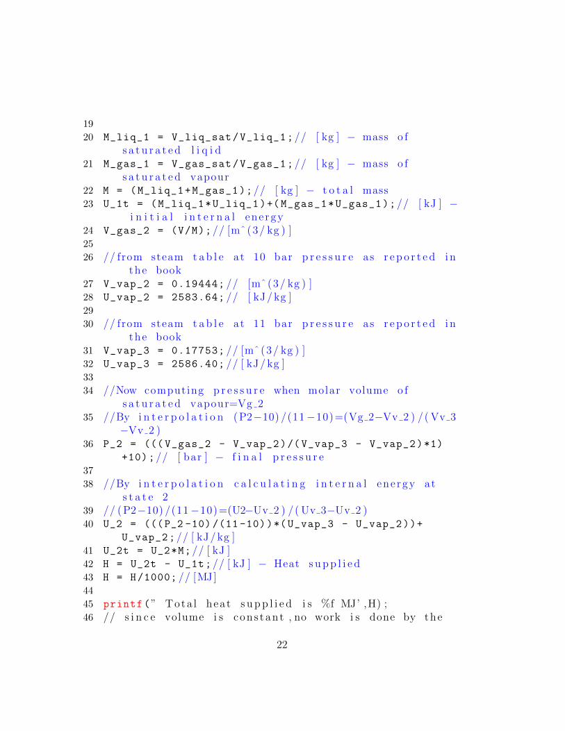
19

20 M_liq_1 = V_liq_sat/V_liq_1;// [ kg ] − mass o fs a t u r a t e d l i q i d

21 M_gas_1 = V_gas_sat/V_gas_1;// [ kg ] − mass o fs a t u r a t e d vapour

22 M = (M_liq_1+M_gas_1);// [ kg ] − t o t a l mass23 U_1t = (M_liq_1*U_liq_1)+( M_gas_1*U_gas_1);// [ kJ ] −

i n i t i a l i n t e r n a l ene rgy24 V_gas_2 = (V/M);// [mˆ(3/ kg ) ]25

26 // from steam t a b l e at 10 bar p r e s s u r e as r e p o r t e d i nthe book

27 V_vap_2 = 0.19444; // [mˆ(3/ kg ) ]28 U_vap_2 = 2583.64; // [ kJ/ kg ]29

30 // from steam t a b l e at 11 bar p r e s s u r e as r e p o r t e d i nthe book

31 V_vap_3 = 0.17753; // [mˆ(3/ kg ) ]32 U_vap_3 = 2586.40; // [ kJ/ kg ]33

34 //Now computing p r e s s u r e when molar volume o fs a t u r a t e d vapour=Vg 2

35 //By i n t e r p o l a t i o n ( P2−10) /(11−10)=(Vg 2−Vv 2 ) /( Vv 3−Vv 2 )

36 P_2 = ((( V_gas_2 - V_vap_2)/( V_vap_3 - V_vap_2)*1)

+10);// [ bar ] − f i n a l p r e s s u r e37

38 //By i n t e r p o l a t i o n c a l c u l a t i n g i n t e r n a l ene rgy ats t a t e 2

39 // ( P2−10) /(11−10)=(U2−Uv 2 ) /( Uv 3−Uv 2 )40 U_2 = (((P_2 -10) /(11 -10))*( U_vap_3 - U_vap_2))+

U_vap_2;// [ kJ/ kg ]41 U_2t = U_2*M;// [ kJ ]42 H = U_2t - U_1t;// [ kJ ] − Heat s u p p l i e d43 H = H/1000; // [MJ]44

45 printf(” Tota l heat s u p p l i e d i s %f MJ’ ,H) ;46 // s i n c e volume i s cons tant , no work i s done by the

22

system and heat s u p p l i e d i s used i n i n c r e a s i n gthe i n t e r n a l ene rgy o f the system .

Scilab code Exa 1.9 Calculation of saturation temperature

1 clear;

2 clc;

3


8 // Given9 // Anto ine e q u a t i o n f o r water l n ( Psat )

=16 .262 − (3799 .89/( T sat + 2 2 6 . 3 5 ) )10 P = 2; // [ atm ] − P r e s s u r e11 P = (2*101325) /1000; // [ kPa ]12

13 P_sat = P;// S a t u r a t i o n p r e s s u r e14 T_sat = (3799.89/(16.262 - log(P_sat))) -226.35; // [C ] −

S a t u r a t i o n t empera tu r e15 // Thus b o i l i n g at 2 atm o c c u r s at Tsat = 1 2 0 . 6 6 C.16

17 //From steam t a b l e s , a t 2 bar , Tsat = 1 2 0 . 2 3 C and at2 . 2 5 bar , Tsat = 1 2 4 . 0 C

18 //From i n t e r p o l a t i o n f o r T sat = 1 2 0 . 6 6 C, P = 2 . 0 2 6 5bar

19 // For P = 2 . 0 2 6 5 bar , T sat , from steam t a b l e byi n t e r p o l a t i o n i s g i v e n by

20 // ( (2 . 0265 −2) /(2 .25 −2) ) =(( Tsat −120 .23)/ (124 . 0 −120 . 23 ) )

21 T_sat_0 = (((2.0265 -2) /(2.25 -2))*(124.0 -120.23))

+120.23; // [C ]22

23 printf(” S a t u r a t i o n t empera tu r e ( Tsat ) = %f C which

23

i s c l o s e to %f C as dete rmined from Anto inee q u a t i o n ”,T_sat_0 ,T_sat);

Scilab code Exa 1.10 Calculation of pressure and temperature at triplepoint

1 clear;

2 clc;

3

4 // Example − 1 . 1 05 // Page number − 276 printf(” Example − 1 . 1 0 and Page number − 27\n\n”);7

8 // Given9 // l o g (P) =−(1640/T) +10.56 ( s o l i d )10 // l o g (P) =−(1159/T) +7.769 ( l i q u i d ) , where T i s i n K11 // F+P=C+2, at t r i p l e p o i n t F+3=1+2 or , F=0 i . e ,

vapour p r e s s u r e o f l i q u i d and s o l i d at t r i p l ep o i n t a r e same , we ge t

12 // −(1640/T) +10.56 = −(1159/T) +7.76913

14 T = (1640 -1159) /(10.56 -7.769);// [K]15 P = 10^(( -1640/T)+10.56);// [ t o r r ]16

17 printf(” The tempera tu r e i s %f K\n”,T);18 printf(” The p r e s s u r e i s %f t o r r ( or mm Hg) ”,P);

Scilab code Exa 1.11 Determination of value of R Cp0 and Cv0

1 clear;

2 clc;

3

4 // Example − 1 . 1 1

24

5 // Page number − 296 printf(” Example − 1 . 1 1 and Page number − 29\n\n”);7

8 // Given9 M_O2 = 31.999; // m o l e c u l a r we ight o f oxygen10 M_N2 = 28.014; // m o l e c u l a r we ight o f n i t r o g e n11 Y = 1.4; // molar heat c a p a c i t i e s r a t i o f o r a i r12

13 // Mo l e cu l a r we ight o f a i r (21 vol% O2 and 79 vol% N2)i s g i v e n by

14 M_air = (0.21* M_O2)+(0.79* M_N2);// ( vol% = mol%)15

16 R = 8.314; // [ J/mol∗K] − U n i v e r s a l gas c o n s t a n t17 R = (R*1/ M_air);// [ kJ/ kg∗K]18

19 printf(” The v a l u e o f u n i v e r s a l gas c o n s t a n t (R) =%f kJ/kg−K \n”,R);

20

21 //Y=Cp0/Cv0 and Cp0−Cv0=R22 Cv_0 = R/(Y-1);// [ kJ/ kg∗K]23 Cp_0 = Y*Cv_0;// [ kJ/ kg∗K]24 printf(” The v a l u e o f Cp 0 f o r a i r i s %f kJ/kg−K\n ’ ,

Cp 0 ) ;25 p r i n t f ( ” The value of Cv_0 for air is %f kJ/kg -K’,

Cv_0);

Scilab code Exa 1.12 Calculation of molar heat capacity

1 clear;

2 clc;

3


25

8 // Given9 Y = 1.4; // molar heat c a p a c i t i e s r a t i o f o r a i r10 R = 8.314; // [ J/mol∗K] − U n i v e r s a l gas c o n s t a n t11 Cv_0 = R/(Y-1);// [ J/mol∗K]12 Cp_0 = Y*Cv_0;// [ J/mol∗K]13

14 printf(” The molar heat c a p a c i t y at c o n s t a n t volume( Cv 0 ) i s %f J/mol−K\n ’ , Cv 0 ) ;

15 p r i n t f ( ” The molar heat capacity at constant

pressure (Cp_0) is %f J/mol -K’,Cp_0);

Scilab code Exa 1.13 Determination of mean heat capacity

1 clear;

2 clc;

3


8 // Given9 // Cp0 =7.7+(0.04594∗10ˆ(−2) ∗T) +(0.2521∗10ˆ(−5) ∗Tˆ ( 2 )

) −(0.8587∗10ˆ(−9) ∗Tˆ ( 3 ) )10 T_1 = 400; // [K]11 T_2 = 500; // [K]12

13 // (C) avg = q /( T 2 − T 1 ) = 1/( T 2 − T 1 ) ∗{ ( i n t e g r a t e( ’C’ , ’ T’ , T 1 , T 2 ) ) }

14 // ( Cp0 ) avg = 1/( T 2 − T 1 ) ∗{ ( i n t e g r a t e ( ’ Cp0 ’ , ’ T’ , T 1, T 2 ) ) }

15 Cp0_avg = (1/( T_2 - T_1))*integrate( ’7 . 7+(0 .04594∗10ˆ( −2) ∗T) +(0.2521∗10ˆ(−5) ∗Tˆ ( 2 ) )−(0.8587∗10ˆ(−9) ∗Tˆ ( 3 ) ) ’ , ’T ’ ,T_1 ,T_2);

16

17 printf(” The mean heat c a p a c i t y ( Cp0 avg ) f o r

26

t eme ra tu r e range o f 400 to 500 K i s %f c a l /mol−K”,Cp0_avg);

Scilab code Exa 1.14 Calculation of enthalpy of water

1 clear;

2 clc;

3


8 // Given9 // ( a )10 P_1 = 0.2; // [MPa] − p r e s s u r e11 x_1 = 0.59; // mole f r a c t i o n12

13 //From s a t u r a t e d steam t a b l e s at 0 . 2 MPa14 H_liq_1 = 504.7; // [ kJ/ kg ] − Enthalpy o f s a t u r a t e d

l i q u i d15 H_vap_1 = 2706.7; // [ kJ/ kg ]− Enthalpy o f s a t u r a t e d

vapour16 H_1 = (H_liq_1 *(1-x_1))+(x_1*H_vap_1);// [ kJ/ kg ]17 printf(” ( a ) . Enthalpy o f 1 kg o f water i n tank i s %f

kJ/ kg\n”,H_1);18

19 // ( b )20 T_2 = 120.23; // [C ] − t empera tu re21 V_2 = 0.6; // [mˆ ( 3 ) / kg ] − s p e c i f i c volume22

23 //From s a t u r a t e d steam t a b l e s at 1 2 0 . 2 3 C, asr e p o r t e d i n the book

24 V_liq_2 =0.001061; // [mˆ ( 3 ) / kg ]25 V_vap_2 =0.8857; // [mˆ ( 3 ) / kg ]26 // s i n c e V 2 < Vv 2 , d r y n e s s f a c t o r w i l l be g i v e n by ,

27

V = ((1−x ) ∗V l i q ) +(x∗V vap )27 x_2 = (V_2 - V_liq_2)/( V_vap_2 - V_liq_2);

28

29 //From steam t a b l e , a t 1 2 0 . 2 C, the vapour p r e s s u r e o fwater i s 0 . 2 MPa. So , en tha lpy i s g i v e n by

30 H_2 = (H_liq_1 *(1-x_2))+( H_vap_1*x_2);// kJ/ kg ]31 printf(” ( b ) . Enthalpy o f s a t u r a t e d steam i s %f kJ/ kg

\n”,H_2);32

33 // ( c )34 P_3 = 2.5; // [MPa]35 T_3 = 350; // [C ]36 //From steam t a b l e s at 2 . 5 MPa, T sat = 2 2 3 . 9 9 C, as

r e p o r t e d i n the book37 // s i n c e , T 3 > Tsat , steam i s s u p e r h e a t e d38 printf(” ( c ) . As steam i s supe rhea ted , from steam

t a b l e , en tha lpy (H) i s 3 1 2 6 . 3 kJ/ kg\n”);39

40 // ( d )41 T_4 = 350; // [C ]42 V_4 = 0.13857; // [mˆ ( 3 ) / kg ]43 //From steam t a b l e , a t 350 C, V l i q = 0 . 0 0 1 7 4 0 mˆ ( 3 ) /

kg and V vap = 0 . 0 0 8 8 1 3 mˆ ( 3 ) / kg . S ince ,V > V vap ,t h e r e f o r e i t i s s u p e r h e a t e d .

44 //From steam t a b l e at 350 C and 1 . 6 MPa, V = 0 . 1 7 4 5 6mˆ ( 3 ) / kg

45 //At 350 C and 2 . 0 MPa, V = 0 . 1 3 8 5 7 mˆ ( 3 ) / kg . So ,46 printf(” ( d ) . The en tha lpy o f s u p e r h e a t e d steam (H)

i s 3 1 3 7 . 0 kJ/ kg\n”);47

48 // ( e )49 P_4 = 2.0; // [MPa]50 U_4 = 2900; // [ kJ/ kg ] − i n t e r n a l ene rgy51 //From s a t u r a t e d t a b l e at 2 . 0 MPa, U l i q = 9 0 6 . 4 4 kJ

and U vap = 2 6 0 0 . 3 kJ/ kg52 // s c i n c e , U 4 > Uv , i t i s s a t u r a t e d .53 //From s u p e r h e a t e d steam t a b l e at 2 . 0 MPa and 350 C,

as r e p o r t e d i n the book

28

54 U_1 = 2859.8; // [ kJ/ kg ]55 H_1 = 3137.0; // [ kJ/ kg ]56 //At 2 . 0 MPa and 400 C,57 U_2 = 2945.2; // [ kJ/ kg ]58 H_2 = 3247.6; // [ kJ/ kg ]59 T = (((U_4 - U_1)/(U_2 - U_1))*(400 - 350)) + 350; //

[C ] − By i n t e r p o l a t i o n60 H = (((T - 350) /(400 - 350))*(H_2 - H_1)) + H_1;// [

kJ/ kg ]61 printf(” ( e ) . The en tha lpy v a l u e ( o f s u p e r h e a t e d

steam ) o b t a i n e d a f t e r i n t e r p o l a t i o n i s %f kJ/ kg\n”,H);

62

63 // ( f )64 P_5 = 2.5; // [MPa]65 T_5 = 100; // [C ]66 //At 100 C, P sa t =101350 N/mˆ ( 2 ) . S i n c e P 5 > P sat ,

i t i s compressed l i q u i d67 P_sat = 0.101350; // [MPa]68 H_liq = 419.04; // [ kJ/ kg ] − At 100 C and 0 . 1 0 1 3 5 MPa69 V_liq = 0.001044; // [mˆ ( 3 ) / kg ] − At 100 C and 0 . 1 0 1 3 5

MPa70 H_0 = H_liq + (V_liq*(P_5 - P_sat))*1000; // kJ/ kg ]71 printf(” ( f ) . The en tha lpy o f compressed l i q u i d i s %f

kJ/ kg\n”,H_0);

29

Chapter 2

Equations of state

Scilab code Exa 2.1 Relations in virial coefficients

1 clear;

2 clc;

3


8 // This problem i n v o l v e s p rov ing a r e l a t i o n i n whichno n um e r i c a l components a r e i n v o l v e d .

9 // For prove r e f e r to t h i s example 2 . 1 on page number40 o f the book .

10 printf(” This problem i n v o l v e s p rov ing a r e l a t i o n i nwhich no n u me r i c a l components a r e i n v o l v e d . \ n\n”

);

11 printf(” For prove r e f e r to t h i s example 2 . 1 on pagenumber 40 o f the book . ”);

Scilab code Exa 2.2 Determination of acentric factor

30

1 clear;

2 clc;

3


8 // Given9 Tc = 647.1; // [K] − C r i t i c a l t empera tu r e

10 Pc = 220.55; // [ bar ] − C r i t i c a l p r e s s u r e11 Tr = 0.7; // Reduced tempera tu r e12

13 T = Tr*Tc;// [K]14 //From steam t a b l e , vapour p r e s s u r e o f H2O at T i s

1 0 . 0 2 [ bar ] , a s r e p o r t e d i n the book15 P = 10.02; // [ bar ]16 w = -1-log10((P/Pc));

17 printf(” The a c e n t r i c f a c t o r (w) o f water at g i v e nc o n d i t i o n i s %f ”,w);

Scilab code Exa 2.3 Calculation of acentric factor

1 clear;

2 clc;

3


8 // Given9 // l o g 1 0 ( Psat ) =8.1122 − (1592 .864/( t +226 .184) ) // ’ Psat ’

i n [mm Hg ] and ’ t ’ i n [ c ]10 Tc = 513.9; // [K] − C r i t i c a l t empera tu r e11 Pc = 61.48; // [ bar ] − C r i t i c a l p r e s s u r e12 Pc = Pc *10^(5);// [N/mˆ ( 2 ) ]

31

13 Tr = 0.7; // Reduced tempera tu r e14

15 T = Tr*Tc;// [K] − Temperature16 T = T - 273.15; // [C ]17 P_sat = 10^(8.1122 - (1592.864/(T + 226.184)));// [mm

Hg ]18 P_sat = (P_sat /760) *101325; // [N/mˆ ( 2 ) ]19 Pr_sat = P_sat/Pc;

20 w = -1-log10(Pr_sat);// A c e n t r i c f a c t o r21 printf(” The a c e n t r i c f a c t o r (w) f o r e t h a n o l at

g i v e n c o n d i t i o n i s %f”,w);

Scilab code Exa 2.4 Calculation of virial coefficients

1 clear;

2 clc;

3


8 // Given9 T = 380; // [K] − Temperature10 Tc = 562.1; // [K] − C r i t i c a l t empera tu r e11 P = 7; // [ atm ] − P r e s s u r e12 P = P*101325; // [N/mˆ ( 2 ) ]13 Pc = 48.3; // [ atm ] − C r i t i c a l p r e s s u r e14 Pc = Pc *101325; // [N/mˆ ( 2 ) ]15 R = 8.314; // [ J/mol∗K] − U n i v e r s a l gas c o n s t a n t16 w = 0.212; // a c e n t r i c f a c t o r17 Tr = T/Tc;// Reduced tempera tu r e18

19 B_0 = 0.083 -(0.422/( Tr)^(1.6));

20 B_1 = 0.139 -(0.172/( Tr)^(4.2));

21

32

22 //We know , ( B∗Pc ) /(R∗Tc ) = B 0+(w∗B 1 )23 B = ((B_0+(w*B_1))*(R*Tc))/Pc;// [mˆ ( 3 ) /mol ]24 printf(” The second v i r i a l c o e f f i c i e n t f o r benzene

i s %e mˆ ( 3 ) /mol\n”,B);25

26 // C o m p r e s s i b i l i t y f a c t o r i s g i v e n by27 Z = 1 + ((B*P)/(R*T));

28 printf(” The c o m p r e s s i b i l i t y f a c t o r at 380 K i s %f\n”,Z);

29

30 //We know tha r Z=(P∗V) /(R/∗T) , t h e r f o r e31 V = (Z*R*T)/P;// [mˆ ( 3 ) /mol ]32 printf(” The molar volume i s %e mˆ ( 3 ) /mol\n”,V);

Scilab code Exa 2.5 Calculation of mass using virial equation of state

1 clear;

2 clc;

3


8 // Given9 V_1 = 0.3; // [mˆ ( 3 ) ] / / volume o f c y l i n d e r10 T = 60+273.15; // [K] − Temperature11 P = 130*10^(5);// [N/mˆ ( 2 ) ] − P r e s s u r e12 Tc = 305.3; // [K] − C r i t i c a l t empera tu r e13 Pc = 48.72*10^(5);// [N/mˆ ( 2 ) ] − C r i t i c a l p r e s s u r e14 w = 0.100; // a c e n t r i c f a c t o r15 M = 30.07; // m o l e c u l a r we ight o f e thane16 Tr = T/Tc;// Reduced tempera tu r e17 R = 8.314; // [ J/mol∗K] − U n i v e r s a l gas c o n s t a n t18

19 B_0 = 0.083 -(0.422/( Tr)^(1.6));

33

20 B_1 = 0.139 -(0.172/( Tr)^(4.2));

21

22 //We know , ( B∗Pc ) /(R∗Tc ) = B 0+(w∗B 1 )23 B = ((B_0 + (w*B_1))*(R*Tc))/Pc;// [mˆ ( 3 ) /mol ] −

Second v i r i a l c o e f f i c i e n t24 Z = 1 + ((B*P)/(R*T));// C o m p r e s s i b i l i t y f a c t o r25 V = (Z*R*T)/P;// [mˆ ( 3 ) /mol ] − Molar volume26

27 //No . o f moles i n 0 . 3 mˆ ( 3 ) c y l i n d e r i s g i v e n by28 n1 = V_1/V;// [ mol ]29

30 // Mass o f gas i n c y l i n d e r i s g i v e n by31 m1 = (n1*M)/1000; // [ kg ]32 printf(” Under a c t u a l c o n d i t i o n s , the mass o f e thane

i s , %f kg\n”,m1);33

34 // Under i d e a l c o n d i t i o n , t a k i n g Z = 1 ,35 V_ideal = (R*T)/P;// [mˆ ( 3 ) /mol ]36 n2 = V_1/V_ideal;// [ mol ]37 m2 = (n2*M)/1000; // [ kg ]38 printf(” Under i d e a l c o n d i t i o n s , the mass o f e thane

i s , %f kg\n”,m2);

Scilab code Exa 2.6 Calculation of molar volume

1 clear;

2 clc;

3 funcprot (0);

4


9 // Given10 T = 373.15; // [K] − Temperature

34

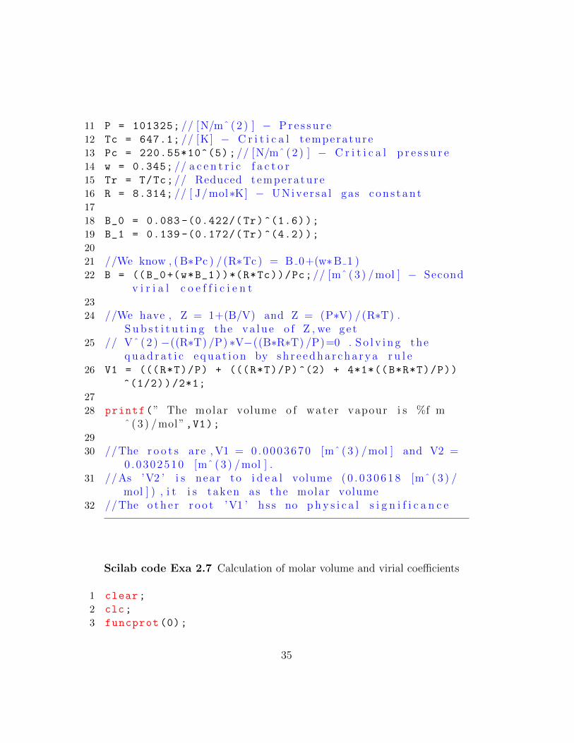
11 P = 101325; // [N/mˆ ( 2 ) ] − P r e s s u r e12 Tc = 647.1; // [K] − C r i t i c a l t empera tu r e13 Pc = 220.55*10^(5);// [N/mˆ ( 2 ) ] − C r i t i c a l p r e s s u r e14 w = 0.345; // a c e n t r i c f a c t o r15 Tr = T/Tc;// Reduced tempera tu r e16 R = 8.314; // [ J/mol∗K] − UNive r sa l gas c o n s t a n t17

18 B_0 = 0.083 -(0.422/( Tr)^(1.6));

19 B_1 = 0.139 -(0.172/( Tr)^(4.2));

20

21 //We know , ( B∗Pc ) /(R∗Tc ) = B 0+(w∗B 1 )22 B = ((B_0+(w*B_1))*(R*Tc))/Pc;// [mˆ ( 3 ) /mol ] − Second

v i r i a l c o e f f i c i e n t23

24 //We have , Z = 1+(B/V) and Z = (P∗V) /(R∗T) .S u b s t i t u t i n g the v a l u e o f Z , we g e t

25 // Vˆ ( 2 ) −((R∗T) /P) ∗V−((B∗R∗T) /P)=0 . S o l v i n g theq u a d r a t i c e q u a t i o n by s h r e e d h a r c h a r y a r u l e

26 V1 = (((R*T)/P) + (((R*T)/P)^(2) + 4*1*((B*R*T)/P))

^(1/2))/2*1;

27

28 printf(” The molar volume o f water vapour i s %f mˆ ( 3 ) /mol”,V1);

29

30 //The r o o t s are , V1 = 0 . 00 0 3 6 7 0 [mˆ ( 3 ) /mol ] and V2 =0 . 0 3 02 5 1 0 [mˆ ( 3 ) /mol ] .

31 //As ’V2 ’ i s near to i d e a l volume ( 0 . 0 3 0 6 1 8 [mˆ ( 3 ) /mol ] ) , i t i s taken as the molar volume

32 //The o t h e r r o o t ’V1 ’ h s s no p h y s i c a l s i g n i f i c a n c e

Scilab code Exa 2.7 Calculation of molar volume and virial coefficients

1 clear;

2 clc;

3 funcprot (0);

35

4


9 // Given10 T = 50+273.15; // [K] − Temperature11 P = 15*10^(5);// [N/mˆ ( 2 ) ] − P r e s s u r e12 Tc = 305.3; // [K] − C r i t i c a l t empera tu r e13 Pc = 48.72*10^(5);// [N/mˆ ( 2 ) ] − C r i t i c a l p r e s s u r e14 w = 0.100; // A c e n t r i c f a c t o r15 B = -157.31; // [ cm ˆ ( 3 ) /mol ] − s econd v i r i a l

c o e f f i c i e n t16 B = B*10^( -6);// [mˆ ( 3 ) /mol ]17 C = 9650; // [ cm ˆ ( 6 ) /mol ˆ ( 2 ) ] − t h i r d v i r i a l

c o e f f i c i e n t18 C = C*10^( -12);// [ cm ˆ ( 6 ) /mol ˆ ( 2 ) ]19 R = 8.314; // [ J/mol∗K] − U n i v e r s a l gas c o n s t a n t20

21 // ( 1 )22 V_1 = (R*T)/P;// [mˆ ( 3 ) /mol ] − Molar volume23 printf(” ( 1 ) . The molar volume f o r i d e a l e q u a t i o n o f

s t a t e i s %e mˆ ( 3 ) /mol\n”,V_1);24

25 // ( 2 )26 Tr = T/Tc;// Reduced tempera tu r e27 // At t h i s t empera tu r e28 B_0 = 0.083 -(0.422/( Tr)^(1.6));

29 B_1 = 0.139 -(0.172/( Tr)^(4.2));

30

31 // We know , ( B∗Pc ) /(R∗Tc ) = B 0+(w∗B 1 )32 B_2 = ((B_0 + (w*B_1))*(R*Tc))/Pc;// [mˆ ( 3 ) /mol ] / /

second v i r i a l c o e f f i c i e n t33 printf(” ( 2 ) . The second v i r i a l c o e f f i c e n t u s i n g

P i t z e r c o r r e l a t i o n i s found to be %e mˆ ( 3 ) /molwhich i s same as g i v e n v a l u e \n”,B_2);

34

35 // ( 3 )

36

36 // Given ( v i r i a l e q u a t i o n ) ,Z=1+(B/V)37 V_3 = B + (R*T)/P;// [mˆ ( 3 ) /mol ] − Molar volume38 printf(” ( 3 ) . The molar volume u s i n g v i r i a l e q u a t i o n

o f s t a t e i s %e mˆ ( 3 ) /mol\n”,V_3);39

40 // ( 4 )41 // Given ( v i r i a l e q u a t i o n ) ,Z = 1 + ( (B∗P) /(R∗T) ) +

( (C − Bˆ ( 2 ) ) /(R∗T) ˆ ( 2 ) ) ∗Pˆ ( 2 )42 V_4 = B + (R*T)/P + ((C - B^(2))/(R*T))*P;// [mˆ ( 3 ) /

mol ]43 printf(” ( 4 ) . The molar volume u s i n g g i v e n v i r i a l

e q u a t i o n o f s t a t e i s %e mˆ ( 3 ) /mol\n”,V_4);44

45 // ( 5 )46 // Given , Z = 1 + (B/V)47 // Also , Z = (P∗V) /(R∗T) . S u b s t i t u t i n g the v a l u e o f Z

, we ge t48 // Vˆ ( 2 ) −((R∗T) /P) ∗V−((B∗R∗T) /P) =0. S o l v i n g the

q u a d r a t i c e q u a t i o n49 deff( ’ [ y ]= f (V) ’ , ’ y=Vˆ ( 2 ) −((R∗T) /P) ∗V−((B∗R∗T) /P) ’ );50 V_5_1 = fsolve(0,f);

51 V_5_2 = fsolve(1,f);

52

53 printf(” ( 5 ) . The molar volume u s i n g g i v e n v i r i a le q u a t i o n o f s t a t e i s %e mˆ ( 3 ) /mol\n”,V_5_2);

54

55 // The r o o t s are , V 5 1 =0.0001743 [mˆ ( 3 ) /mol ] andV 5 2 =0.0016168 [mˆ ( 3 ) /mol ] .

56 // As ’ V 2 ’ i s near to i d e a l volume ( 0 . 0 0 1 7 9 1 1 [mˆ ( 3 ) /mol ] ) , i t i s taken as the molar volume

57

58 // ( 6 )59 // Given , Z = 1 + (B/V) + (C/Vˆ ( 2 ) )60 // Also , Z = (P∗V) /(R∗T) . S u b s t i t u t i n g the v a l u e o f Z

, we ge t61 // Vˆ ( 3 ) −((R∗T) /P) ∗Vˆ ( 2 ) −((B∗R∗T) /P) ∗V−((C∗R∗T) /P)

=0. S o l v i n g the c u b i c e q u a t i o n62 deff( ’ [ y ]= f 1 (V) ’ , ’ y=Vˆ ( 3 ) −((R∗T) /P) ∗Vˆ ( 2 ) −((B∗R∗T) /P

37

) ∗V−((C∗R∗T) /P) ’ );63 V_6_3=fsolve(-1,f1);

64 V_6_4=fsolve(0,f1);

65 V_6_5=fsolve(1,f1);

66 //The above e q u a t i o n has 1 r e a l and 2 imag inaryr o o t s . We c o n s i d e r on ly r e a l r o o t .

67 printf(” ( 6 ) . The molar volume u s i n g g i v e n v i r i a le q u a t i o n o f s t a t e i s %e mˆ ( 3 ) /mol\n”,V_6_5);

Scilab code Exa 2.8 Determination of second and third virial coefficients

1 clear;

2 clc;

3 funcprot (0);

4


9 // Given10 T = 0 + 273.15; // [K] − Temperature11 R = 8.314; // [ J/mol∗K] − U n i v e r s a l gas c o n s t a n t12

13 // V i r i a l e q u a t i o n o f s t a t e , Z=1+(B/V) +(C/Vˆ ( 2 ) )14 //From above e q u a t i o n we g e t (Z−1)∗V=B+(C/V)15

16 P=[50 ,100 ,200 ,400 ,600 ,1000];

17 Z=[0.9846 ,1.0000 ,1.0365 ,1.2557 ,1.7559 ,2.0645];

18 V=zeros (6);

19 k=zeros (6);

20 t=zeros (6);

21 for i=1:6;

22 V(i)=(Z(i)*R*T)/(P(i)*101325);// [mˆ ( 3 ) /mol ]23 k(i)=(Z(i) -1)*V(i);

24 t(i)=1/V(i);

38

25 end

26 [C,B,sig]= reglin(t’,k’);

27

28 //From the r e g r e s s i o n , we g e t i n t e r c e p t=B and s l o p e=C, and thus ,

29 printf(” The v a l u e o f s econd v i r i a l c o e f f i c i e n t (B)i s %e mˆ ( 3 ) /mol\n”,B);

30 printf(” The v a l u e o f t h i r d v i r i a l c o e f f i c i e n t (C)i s %e mˆ ( 6 ) /mol ˆ ( 2 ) ”,C);

Scilab code Exa 2.9 Estimation of second virial coefficient

1 clear;

2 clc;

3


8 // Given9 T = 444.3; // [K] − Temperature10 R = 8.314; // [ J/mol∗K] − U n i v e r s a l gas c o n s t a n t11 B_11 = -8.1; // [ cm ˆ ( 3 ) /mol ]12 B_11 = -8.1*10^( -6);// [mˆ ( 3 ) /mol ]13 B_22 = -293.4*10^( -6);// [mˆ ( 3 ) /mol ]14 y1 = 0.5; // mole f r a c t i o n // equ imo l a r mixture15 y2 = 0.5;

16

17 // For component 1 ( methane )18 Tc_1 = 190.6; // [K] − c r i c i t i c a l t empera tu r e19 Vc_1 = 99.2; // [ cm ˆ ( 3 ) /mol ] − c r i c i t i c a l molar volume20 Zc_1 = 0.288; // c r i t i c a l c o m p r e s s i b i l i t y f a c t o r21 w_1 = 0.012; // a c e n t r i c f a c t o r22

23 // For component 2 ( n−butane )

39

24 Tc_2 = 425.2; // [K]25 Vc_2 = 255.0; // [ cm ˆ ( 3 ) /mol ]26 Zc_2 = 0.274;

27 w_2 = 0.199;

28

29 // Using v i r i a l mix ing r u l e , we ge t30 Tc_12 = (Tc_1*Tc_2)^(1/2);// [K]31 w_12 = (w_1 + w_2)/2;

32 Zc_12 = (Zc_1+Zc_2)/2;

33 Vc_12 = ((( Vc_1)^(1/3) + (Vc_2)^(1/3))/2) ^(3);// [ cmˆ ( 3 ) /mol ]

34 Vc_12 = Vc_12 *10^( -6);// [ cm ˆ ( 3 ) /mol ]35 Pc_12 = (Zc_12*R*Tc_12)/Vc_12;// [N/mˆ ( 2 ) ]36 Tr_12 = T/Tc_12;// Reduced tempera tu r e37 B_0 = 0.083 - (0.422/( Tr_12)^(1.6));

38 B_1 = 0.139 - (0.172/( Tr_12)^(4.2));

39

40 //We know , ( B 12∗Pc 12 ) /(R∗Tc 12 ) = B 0 + ( w 12∗B 1 )41 B_12 = ((B_0+(w_12*B_1))*(R*Tc_12))/Pc_12;// [mˆ ( 3 ) /

mol ] − Cross c o e f f i c i e n t42 B = y1^(2)*B_11 +2*y1*y2*B_12+y2^(2)*B_22;// [mˆ ( 3 ) /

mol ] − Second v i r i a l c o e f f i c i e n t f o r mixture43 B = B*10^(6);// [ cm ˆ ( 3 ) /mol ]44 printf(” The second v i r i a l c o e f f i c i e n t , ( B) f o r the

mixture o f gas i s %f cm ˆ ( 3 ) /mol”,B);

Scilab code Exa 2.10 Estimation of molar volume

1 clear;

2 clc;

3


40

8 // Given9 T = 71+273.15; // [K] − Temperature10 P = 69*10^(5);// [N/mˆ ( 2 ) ] − P r e s s u r e11 y1 = 0.5; // [ mol ] − mole f r a c t i o n o f equ imo l a r

mixture12 y2 = 0.5;

13 R = 8.314; // [ J/mol∗K] − U n i v e r s a l gas c o n s t a n t14

15 // For component 1 ( methane )16 Tc_1 =190.6; // [K] − C r i t i c a l t empera tu r e17 Pc_1 = 45.99*10^(5);// [N/mˆ ( 2 ) ] − C r i t i c a l p r e s s u r e18 Vc_1 = 98.6; // [ cm ˆ ( 3 ) /mol ] − C r i t i c a l volume19 Zc_1 = 0.286; // C r i t i c a l c o m p r e s s i b i l i t y f a c t o r20 w_1 = 0.012; // a c e n t r i c f a c t o r21

22 // For component 2 ( hydrogen s u l p h i d e )23 Tc_2 = 373.5; // [K]24 Pc_2 = 89.63*10^(5);// [N/mˆ ( 2 ) ]25 Vc_2 = 98.5; // [ cm ˆ ( 3 ) /mol ]26 Zc_2 = 0.284;

27 w_2 = 0.094;

28

29 // For component 130 Tr_1 = T/Tc_1;// Reduced tempera tu r e31 //At reduced tempera tu r e32 B1_0 = 0.083 -(0.422/( Tr_1)^(1.6));

33 B1_1 = 0.139 -(0.172/( Tr_1)^(4.2));

34 //We know , ( B∗Pc ) /(R∗Tc ) = B 0+(w∗B 1 )35 B_11 = ((B1_0+(w_1*B1_1))*(R*Tc_1))/Pc_1;// [mˆ ( 3 ) /

mol ]36

37 // S i m i l a r l y f o r component 238 Tr_2 = T/Tc_2;// Reduced tempera tu r e39 //At reduced tempera tu r e Tr 2 ,40 B2_0 = 0.083 - (0.422/( Tr_2)^(1.6));

41 B2_1 = 0.139 - (0.172/( Tr_2)^(4.2));

42 B_22 = ((B2_0+(w_2*B2_1))*(R*Tc_2))/Pc_2;// [mˆ ( 3 ) /mol ]

41

43

44 // For c r o s s c o e f f c i e n t45 Tc_12 = (Tc_1*Tc_2)^(1/2);// [K]46 w_12 = (w_1 + w_2)/2;

47 Zc_12 = (Zc_1 + Zc_2)/2;

48 Vc_12 = ((( Vc_1)^(1/3) + (Vc_2)^(1/3))/2) ^(3);// [ cmˆ ( 3 ) /mol ]

49 Vc_12 = Vc_12 *10^( -6);// [mˆ ( 3 ) /mol ]50 Pc_12 = (Zc_12*R*Tc_12)/Vc_12;// [N/mˆ ( 2 ) ]51

52 //Now we have , ( B 12∗Pc 12 ) /(R∗Tc 12 ) = B 0+(w 12∗B 1)

53 // where B 0 and B 1 a r e to be e v a l u a t e d at Tr 1254 Tr_12 = T/Tc_12;

55 //At reduced tempera tu r e Tr 1256 B_0 = 0.083 - (0.422/( Tr_12)^(1.6));

57 B_1 = 0.139 - (0.172/( Tr_12)^(4.2));

58 B_12 =((B_0 + (w_12*B_1))*R*Tc_12)/Pc_12;// [mˆ ( 3 ) /mol]

59

60 // For the mixture61 B = y1^(2)*B_11 +2*y1*y2*B_12 + y2^(2)*B_22;// [mˆ ( 3 ) /

mol ]62

63 //Now g i v e n v i r i a l e q u a t i o n i s , Z=1+(B∗P) /(R∗T)64 Z = 1 + (B*P)/(R*T);

65

66 // Also Z = (P∗V) /(R∗T) . The r e f o r e ,67 V = (Z*R*T)/P;// [mˆ ( 3 ) /mol ]68

69 printf(” The molar volume o f the mixture i s %e mˆ ( 3 )/mol”,V);

70 //The v a l u e o b t a i n e d i s near the e x p e r i m e n t a l v a l u eo f V exp = 3.38∗10ˆ( −4) mˆ ( 3 ) /mol

42

Scilab code Exa 2.11 Calculation of maximum temperature

1 clear;

2 clc;

3 funcprot (0);

4


9 // Given10 P = 6*10^(6);// [ Pa ] − P r e s s u r e11 P_max = 12*10^(6);// [ Pa ] − Max p r e s s u r e to which

c y l i n d e r may be exposed12 T = 280; // [K] − Temperature13 R = 8.314; // [ J/mol∗K] − U n i v e r s a l gas c o n s t a n t14

15 // ( 1 ) . Assuming i d e a l gas behav iour ,16 V_ideal = (R*T)/P;// [mˆ ( 3 ) /mol ]17 //Now when tempera tu r e and p r e s s u r e a r e i n c r e a s e d ,

the molar volume rema ins same , as t o t a l volume andnumber o f moles a r e same .

18 // For max p r e s s u r e o f 12 MPa, t empera tu r e i s19 T_max_ideal = (P_max*V_ideal)/R;

20 printf(” ( 1 ) . The maximum tempera tu r e assuming i d e a lb ehav i ou r i s %f K\n”,T_max_ideal);

21

22 // ( 2 ) . Assuming v i r i a l e q u a t i o n o f s t a t e23 // For component 1 ( methane ) , a t 280 K24 Tc_1 = 190.6; // [K]25 Pc_1 = 45.99*10^(5);// [N/mˆ ( 2 ) ]26 Vc_1 = 98.6; // [ cm ˆ ( 3 ) /mol ]27 Zc_1 = 0.286;

28 w_1 = 0.012;

29 Tr_1 = T/Tc_1;// Reduced tempera tu r e30 B1_0 = 0.083 - (0.422/( Tr_1)^(1.6));

31 B1_1 = 0.139 - (0.172/( Tr_1)^(4.2));

32

43

33 //We know , ( B∗Pc ) /(R∗Tc ) = B 0+(w∗B 1 )34 B_11 = ((B1_0 + (w_1*B1_1))*(R*Tc_1))/Pc_1;// [mˆ ( 3 ) /

mol ]35

36 // For component 2 ( Propane )37 Tc_2 = 369.8; // [K]38 Pc_2 = 42.48*10^(5);// [N/mˆ ( 2 ) ]39 Vc_2 = 200; // [ cm ˆ ( 3 ) /mol ]40 Zc_2 = 0.276;

41 w_2 = 0.152;

42 Tr_2 = T/Tc_2;// Reduced tempera tu r e43 B2_0 = 0.083 - (0.422/( Tr_2)^(1.6));

44 B2_1 = 0.139 - (0.172/( Tr_2)^(4.2));

45 B_22 = ((B2_0 + (w_2*B2_1))*(R*Tc_2))/Pc_2;// [mˆ ( 3 ) /mol ]

46

47 // For c r o s s c o e f f c i e n t48 y1 = 0.8; // mole f r a c t i o n o f component 149 y2 = 0.2; // mole f r a c t i o n o f component 250 Tc_12 = (Tc_1*Tc_2)^(1/2);// [K]51 w_12 = (w_1 + w_2)/2;

52 Zc_12 = (Zc_1 + Zc_2)/2;

53 Vc_12 = ((( Vc_1)^(1/3) + (Vc_2)^(1/3))/2) ^(3);// [ cmˆ ( 3 ) /mol ]

54 Vc_12 = Vc_12 *10^( -6);// [mˆ ( 3 ) /mol ]55 Pc_12 = (Zc_12*R*Tc_12)/Vc_12;// [N/mˆ ( 2 ) ]56 Tr_12 = T/Tc_12;

57

58 //At reduced temperature , Tr 12 ,59 B_0 = 0.083 - (0.422/( Tr_12)^(1.6));

60 B_1 = 0.139 - (0.172/( Tr_12)^(4.2));

61 B_12 = ((B_0 + (w_12*B_1))*R*Tc_12)/Pc_12;// [mˆ ( 3 ) /mol ]

62

63 // For the mixture64 B = y1^(2)*B_11 +2*y1*y2*B_12 + y2^(2)*B_22;// [mˆ ( 3 ) /

mol ]65

44

66 //Now g i v e n v i r i a l e q u a t i o n i s , Z=1+(B∗P) /(R∗T)67 Z = 1 + (B*P)/(R*T);

68 // Also Z = (P∗V) /(R∗T) . The r e f o r e ,69 V_real = (Z*R*T)/P;// [mˆ ( 3 ) /mol ]70

71 // This molar volume rema ins the same as the volumeand number o f moles r ema ins f i x e d .

72 // S i c e Z i s a f u n c t i o n o f p r e s u r e and temperature ,we s h a l l assume a temperature , c a l c u l a t e Z andaga in c a l c u l a t e temperature , t i l l c o n v e r g e n c e i so b t a i n e d .

73 // We w i l l use the concep t o f i t e r a t i o n to computethe c o n v e r g e n t v a l u e o f t empera tu r e

74 // Let us s t a r t with the t empera tu r e at i d e a lc o n d i t i o n s i . e T = 560 K,

75

76 T_prime = 560; // [K]77 fault = 10;

78

79 while(fault > 1)

80 T_prime_r1 = T_prime/Tc_1;

81 B_prime1_0 = 7.7674*10^( -3);

82 B_prime1_1 = 0.13714;

83 B_prime_11 = (( B_prime1_0 + (w_1*B_prime1_1))*(R*

Tc_1))/Pc_1;// [mˆ ( 3 ) /mol ]84

85 // S i m i l a r l y f o r component 2 ,86 T_prime_r2 = T_prime/Tc_2;

87 B_prime2_0 = -0.1343;

88 B_prime2_1 = 0.10887;

89 B_prime_22 = (( B_prime2_0 + (w_2*B_prime2_1))*(R*

Tc_2))/Pc_2;// [mˆ ( 3 ) /mol ]90

91 // For c r o s s c o e f f i c i e n t ( assuming k12 =0)92 // Tc 12 , w 12 , Zc 12 , Vc 12 and Pc 12 have

a l r e a d y been c a l c u l a t e d above , now93 T_prime_r12 = T_prime/Tc_12;//94 //At reduced temperature , T pr ime r12 ,

45

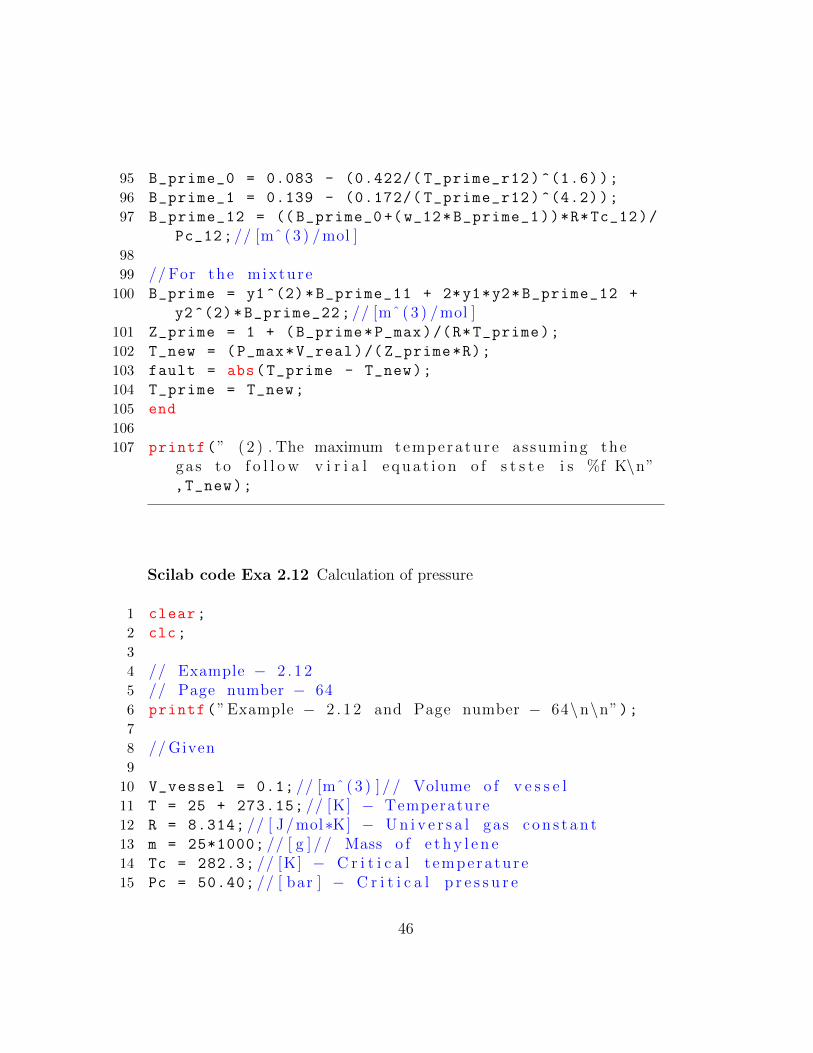
95 B_prime_0 = 0.083 - (0.422/( T_prime_r12)^(1.6));

96 B_prime_1 = 0.139 - (0.172/( T_prime_r12)^(4.2));

97 B_prime_12 = (( B_prime_0 +(w_12*B_prime_1))*R*Tc_12)/

Pc_12;// [mˆ ( 3 ) /mol ]98

99 // For the mixture100 B_prime = y1^(2)*B_prime_11 + 2*y1*y2*B_prime_12 +

y2^(2)*B_prime_22;// [mˆ ( 3 ) /mol ]101 Z_prime = 1 + (B_prime*P_max)/(R*T_prime);

102 T_new = (P_max*V_real)/( Z_prime*R);

103 fault = abs(T_prime - T_new);

104 T_prime = T_new;

105 end

106

107 printf(” ( 2 ) . The maximum tempera tu r e assuming thegas to f o l l o w v i r i a l e q u a t i o n o f s t s t e i s %f K\n”,T_new);

Scilab code Exa 2.12 Calculation of pressure

1 clear;

2 clc;

3


8 // Given9

10 V_vessel = 0.1; // [mˆ ( 3 ) ] / / Volume o f v e s s e l11 T = 25 + 273.15; // [K] − Temperature12 R = 8.314; // [ J/mol∗K] − U n i v e r s a l gas c o n s t a n t13 m = 25*1000; // [ g ] / / Mass o f e t h y l e n e14 Tc = 282.3; // [K] − C r i t i c a l t empera tu r e15 Pc = 50.40; // [ bar ] − C r i t i c a l p r e s s u r e

46

16 Pc = Pc *10^(5);// [N/mˆ ( 2 ) ]17 Zc = 0.281; // C r i t i c a l c o m p r e s s i b i l i t y f a c t o r18 Vc = 131; // [ cm ˆ ( 3 ) /mol ] − C r i t i c a l volume19 Vc = Vc*10^( -6);// [mˆ ( 3 ) /mol ]20 w = 0.087; // A c e n t r i c f a c t o r21 M = 28.054; // Mo l e cu l a r we ight o f e t h y l e n e22

23 n = m/M;// [ mole ] − No . o f moles o f e t h y l e n e24 V = V_vessel/n;// [mˆ ( 3 ) /mol ] − Molar volume25

26 // Under R e d l i c h Kwong e q u a t i o n o f s t a t e , we have27 a = (0.42748*(R^(2))*(Tc ^(2.5)))/Pc;// [ Pa∗mˆ ( 6 ) ∗K

ˆ ( 1 / 2 ) /mol ]28 b = (0.08664*R*Tc)/Pc;// [mˆ ( 3 ) /mol ]29 P = ((R*T)/(V-b))-(a/(T^(1/2)*V*(V+b)));// [N/mˆ ( 2 ) ]30 printf(” The r e q u i r e d p r e s s u r e u s i n g R e d l i c h Kwong

e q u a t i o n o f s t a t e i s %e N/mˆ ( 2 ) \n”,P);31

32 // For i d e a l gas e q u a t i o n o f s t a t e ,33 P_ideal = (R*T)/V;// [N/mˆ ( 2 ) ]34 printf(” For i d e a l gas e q u a t i o n o f s t a t e , the

r e q u i r e d p r e s s u r e i s %e N/mˆ ( 2 ) \n”,P_ideal);


1 clear;

2 clc;

3


8 // Given9

10 V_vessel = 360*10^( -3);// [mˆ ( 3 ) ] − volume o f v e s s e l

47

11 T = 62+273.15; // [K] − Temperature12 R = 8.314; // [ J/mol∗K] − U n i v e r s a l gas c o n s t a n t13 m = 70*1000; // [ g ] / − Mass o f carbon d i o x i d e14

15 // For carbon d i o x i d e16 Tc = 304.2; // [K] − C r i c i t i c a l t empera tu r e17 Pc = 73.83; // [ bar ] − C r i c i t i c a l p r e s s u r e18 Pc = Pc *10^(5);// [N/mˆ ( 2 ) ]19 Zc = 0.274; // C r i t i c a l c o m p r e s s i b i l i t y f a c t o r20 Vc = 94.0; // [ cm ˆ ( 3 ) /mol ]21 Vc = Vc*10^( -6);// [mˆ ( 3 ) /mol ]22 w = 0.224; // A c e n t r i c f a c t o r23 M = 44.01; // Mo l e cu l a r we ight o f carbon d i o x i d e24

25 n = m/M;// [ mol ] − No . o f moles26 V = V_vessel/n;// [mˆ ( 3 ) /mol ] / / molar volume27

28 // ( 1 )29 // I d e a l gas behav i ou r30 P_1 = (R*T)/V;// [N/mˆ ( 2 ) ]31 printf(” ( 1 ) . The r e q u i r e d p r e s s u r e u s i n g i d e a l

e q u a t i o n o f s t a t e i s %e N/mˆ ( 2 ) \n”,P_1);32

33 // ( 2 )34 // V i r i a l e q u a t i o n o f s t a t e , Z = 1 + (B∗P) /(R∗T)35 // (P∗V) /(R∗T) = 1 + (B∗P) /(R∗T) , and thus P = (R∗T)

/(V − B) . Now36 Tr = T/Tc;// Reduced tempera tu r e37 // At reduced tempera tu r e Tr ,38 B_0 = 0.083 - (0.422/( Tr)^(1.6));

39 B_1 = 0.139 - (0.172/( Tr)^(4.2));

40 B = ((B_0 + (w*B_1))*(R*Tc))/Pc;// [mˆ ( 3 ) /mol ]41 P_2 = (R*T)/(V - B);// [N/mˆ ( 2 ) ]42 printf(” ( 2 ) . The r e q u i r e d p r e s s u r e u s i n g g i v e n

v i r i a l e q u a t i o n o f s t a t e i s %e N/mˆ ( 2 ) \n”,P_2);43

44 // ( 3 )45 // V i r i a l e q u a t i o n o f s t a t e , Z = 1 + (B/V)

48

46 // (P∗V) /(R∗T) = 1 + (B/V)47 P_3 = ((R*T)/V) + (B*R*T)/(V^(2));// [N/mˆ ( 2 ) ]48 printf(” ( 3 ) . The r e q u i r e d p r e s s u r e u s i n g g i v e n

v i r i a l e q u a t i o n o f s t a t e i s %e N/mˆ ( 2 ) \n”,P_3);49

50 // ( 4 )51 // Van der Wal ls e q u a t i o n o f s t a t e , P = ( (R∗T) /(V−b ) )

− a /(Vˆ ( 2 ) )52 a = (27*(R^(2))*(Tc^(2)))/(64*Pc);// [ Pa∗mˆ ( 6 ) /mol

ˆ ( 2 ) ]53 b = (R*Tc)/(8*Pc);// [mˆ ( 3 ) /mol ]54 P_4 = ((R*T)/(V-b)) - a/(V^(2));// [N/mˆ ( 2 ) ]55 printf(” ( 4 ) . The r e q u i r e d p r e s s u r e u s i n g van der

Wal ls e q u a t i o n o f s t a t e i s %e N/mˆ ( 2 ) \n”,P_4);56

57 // ( 5 )58 // R e d l i c h Kwong e q u a t i o n o f s t a t e ,59 a_1 = (0.42748*(R^(2))*(Tc ^(2.5)))/Pc;// [ Pa∗mˆ ( 6 ) ∗K

ˆ ( 1 / 2 ) /mol ]60 b_1 = (0.08664*R*Tc)/Pc;// [mˆ ( 3 ) /mol ]61 P_5 = ((R*T)/(V - b_1)) - (a_1/(T^(1/2)*V*(V + b_1))

);// [N/mˆ ( 2 ) ]62 printf(” ( 5 ) . The r e q u i r e d p r e s s u r e u s i n g R e d l i c h

Kwong e q u a t i o n o f s t a t e i s %e N/mˆ ( 2 ) \n”,P_5);

Scilab code Exa 2.14 Determination of compressibility factor

1 clear;

2 clc;

3 funcprot (0);

4


49

9 // Given10 T = 500+273.15; // [K] − Temperature11 R = 8.314; // [ J/mol∗K] − U n i v e r s a l gas c o n s t a n t12 P = 325*1000; // [ Pa ] − P r e s s u r e13 Tc = 647.1; // [K] − C r i c i t i c a l t empera tu r e14 Pc = 220.55; // [ bar ] − C r i c i t i c a l p r e s s u r e15 Pc = Pc *10^(5);// [N/mˆ ( 2 ) ]16

17 // ( 1 )18 // Van der Wal ls e q u a t i o n o f s t a t e ,19 a = (27*(R^(2))*(Tc^(2)))/(64*Pc);// [ Pa∗mˆ ( 6 ) /mol

ˆ ( 2 ) ]20 b = (R*Tc)/(8*Pc);// [mˆ ( 3 ) /mol ]21 // The c u b i c form o f van der Wal ls e q u a t i o n o f s t a t e

i s g i v e n by ,22 // Vˆ ( 3 )−(b+(R∗T) /P) ∗Vˆ ( 2 ) +(a/P) ∗V−(a∗b ) /P=023 // S o l v i n g the c u b i c e q u a t i o n24 deff( ’ [ y ]= f (V) ’ , ’ y=Vˆ ( 3 )−(b+(R∗T) /P) ∗Vˆ ( 2 ) +(a/P) ∗V−(

a∗b ) /P ’ );25 V_1 = fsolve(1,f);

26 V_2 = fsolve (10,f);

27 V_3 = fsolve (100,f);

28 // The above e q u a t i o n has 1 r e a l and 2 imag inaryr o o t s . We c o n s i d e r on ly r e a l root ,

29 Z_1 = (P*V_1)/(R*T);// c o m p r e s s i b i l i t y f a c t o r30 printf(” ( 1 ) . The c o m p r e s s i b i l i t y f a c t o r o f steam

u s i n g van der Wal ls e q u a t i o n o f s t a t e i s %f\n”,Z_1);

31

32 // ( 2 )33

34 // R e d l i c h Kwong e q u a t i o n o f s t a t e ,35 a_1 = (0.42748*(R^(2))*(Tc ^(2.5)))/Pc;// [ Pa∗mˆ ( 6 ) ∗K

ˆ ( 1 / 2 ) /mol ]36 b_1 = (0.08664*R*Tc)/Pc;// [mˆ ( 3 ) /mol ]37 // The c u b i c form o f R e d l i c h Kwong e q u a t i o n o f s t a t e

i s g i v e n by ,38 // Vˆ ( 3 ) −((R∗T) /P) ∗Vˆ ( 2 ) −(( b 1 ˆ ( 2 ) ) +(( b 1 ∗R∗T) /P)−(a

50

/(Tˆ ( 1 / 2 ) ∗P) ) ∗V−(a∗b ) /(Tˆ ( 1 / 2 ) ∗P)=039 // S o l v i n g the c u b i c e q u a t i o n40 deff( ’ [ y ]= f 1 (V) ’ , ’ y=Vˆ ( 3 ) −((R∗T) /P) ∗Vˆ ( 2 ) −(( b 1 ˆ ( 2 ) )

+(( b 1 ∗R∗T) /P)−( a 1 /(Tˆ ( 1 / 2 ) ∗P) ) ) ∗V−( a 1 ∗ b 1 ) /(Tˆ ( 1 / 2 ) ∗P) ’ );

41 V_4=fsolve(1,f1);

42 V_5=fsolve (10,f1);

43 V_6=fsolve (100,f1);


45 // Thus c o m p r e s s i b i l i t y f a c t o r i s46 Z_2 = (P*V_4)/(R*T);// c o m p r e s s i b i l i t y f a c t o r47 printf(” ( 2 ) . The c o m p r e s s i b i l i t y f a c t o r o f steam

u s i n g R e d l i c h Kwong e q u a t i o n o f s t a t e i s %f\n”,Z_2);

Scilab code Exa 2.15 Determination of molar volume

1 clear;

2 clc;

3


8 // Given9 T = 250+273.15; // [K]10 R = 8.314; // [ J/mol∗K]11 P = 39.76; // [ bar ] Vapour p r e s s u r e o f water at T12 P = P*10^(5);// [N/mˆ ( 2 ) ]13 Tc = 647.1; // [K] − C r i c i t i c a l t empera tu r e14 Pc = 220.55*10^(5);// [N/mˆ ( 2 ) ] − C r i c i t i c a l p r e s s u r e15 w = 0.345; // A c e n t r i c f a c t o r16 M = 18.015; // Mo l e cu l a r we ight o f water17

51

18 // Using peng−Robinson e q u a t i o n o f s t s t e19 m = 0.37464 + 1.54226*w - 0.26992*w^(2);

20 Tr = T/Tc;

21 alpha = (1 + m*(1 - Tr ^(1/2)))^(2);

22 a = ((0.45724*(R*Tc)^(2))/Pc)*alpha;// [ Pa∗mˆ ( 6 ) /molˆ ( 2 ) ]

23 b = (0.07780*R*Tc)/Pc;// [mˆ ( 3 ) /mol ]24 // Cubuc form o f Peng−Robinson e q u a t i o n o f s t s t e i s

g i v e n by25 // Vˆ ( 3 ) + ( b−(R∗T) /P) ∗Vˆ ( 2 ) − ( ( 3∗ b ˆ ( 2 ) ) + ( ( 2∗R∗T∗

b ) /P) − ( a/P) ) ∗V+b ˆ ( 3 ) + ( (R∗T∗ ( b ˆ ( 2 ) ) /P) − ( ( a∗b) /P) = 0 ;

26 // S o l v i n g the c u b i c e q u a t i o n27 deff( ’ [ y ]= f (V) ’ , ’ y=Vˆ ( 3 ) +(b−(R∗T) /P) ∗Vˆ ( 2 ) −((3∗b ˆ ( 2 )

) +((2∗R∗T∗b ) /P)−(a/P) ) ∗V+b ˆ ( 3 ) +((R∗T∗ ( b ˆ ( 2 ) ) ) /P)−((a∗b ) /P) ’ );

28 V_1 = fsolve(-1,f);

29 V_2 = fsolve(0,f);

30 V_3 = fsolve(1,f);

31 //The l a r g e s t r o o t i s f o r vapour phase ,32 V_vap = V_3;// [mˆ ( 3 ) /mol ] − Molar volume ( s a t u r a t e d

vapour )33 V_vap = V_vap *10^(6)/M;// [ cm ˆ ( 3 ) /g ]34

35 printf(” The moar volume o f s a t u r a t e d water i n thevapour phase ( V vap ) i s %f cm ˆ ( 3 ) /g\n”,V_vap);

36

37 //The s m a l l e s t r o o t i s f o r l i q u i d phase ,38 V_liq = V_1;// [mˆ ( 3 ) /mol ] − molar volume ( s a t u r a t e d

l i q u i d )39 V_liq = V_liq *10^(6)/M;// [ cm ˆ ( 3 ) /g ]40 printf(” The moar volume o f s a t u r a t e d water i n the

l i q u i d phase ( V l i q ) i s %f cm ˆ ( 3 ) /g\n”,V_liq);41

42 //From steam t a b l e at 250 C, V vap = 5 0 . 1 3 [ cm ˆ ( 3 ) /g] and V l i q = 1 . 2 5 1 [ cm ˆ ( 3 ) /g ] .

43 printf(” From steam t a b l e at 250 C, V vap = 5 0 . 1 3 [cm ˆ ( 3 ) /g ] and V l i q = 1 . 2 5 1 [ cm ˆ ( 3 ) /g ] ”);

52

Scilab code Exa 2.16 Calculation of volume

1 clear;

2 clc;

3 funcprot (0);

4


9 // Given10 T = 500+273.15; // [K] − Temperature11 P = 15; // [ atm ] − P r e s s u r e12 P = P*101325; // [N/mˆ ( 2 ) ]13 R = 8.314; // [ J/mol∗K] − U n i v e r s a l gas c o n s t a n t14 Tc = 190.6; // [K] − C r i c i t i c a l t empera tu r e15 Pc = 45.99*10^(5);// [N/mˆ ( 2 ) ] − C r i c i t i c a l p r e s s u r e16 Vc = 98.6; // [ cm ˆ ( 3 ) /mol ] − C r i c i t i c a l molar volume17 Zc = 0.286; // C r i t i c a l c o m p r e s s i b i l i t y f a c t o r18 w = 0.012; // A c e n t r i c f a c t o r19

20 // ( 1 )21 // V i r i a l e q u a t i o n o f s t a t e , Z = 1 + (B∗P) /(R∗T)22 Tr_1 = T/Tc;// Reduced tempera tu r e23 B_0 = 0.083 -(0.422/( Tr_1)^(1.6));

24 B_1 = 0.139 -(0.172/( Tr_1)^(4.2));

25 // We know , ( B∗Pc ) /(R∗Tc ) = B 0+(w∗B 1 )26 B = ((B_0+(w*B_1))*(R*Tc))/Pc;// [mˆ ( 3 ) /mol ] / / second

v i r i a l c o e f f i c i e n t27 Z = 1 + (B*P)/(R*T);// c o m p r e s s i b i l i t y f a c t o r28 // (P∗V) /(R∗T)=1+(B∗P) /(R∗T) , and thus ,29 V_1 = (Z*R*T)/P;// [mˆ ( 3 ) /mol ]30 printf(” ( 1 ) . The molar volume o f methane u s i n g g i v e n

v i r i a l e q u a t i o n i s %e mˆ ( 3 ) /mol\n”,V_1);

53

31

32 // ( 2 ) .33 // V i r i a l e q u a t i o n o f s t a t e , Z = 1 + (B/V)34 // Also , Z = (P∗V) /(R∗T) . S u b s t i t u t i n g the v a l u e o f Z ,

we g e t35 // Vˆ ( 2 ) − ( (R∗T) /P) ∗V − ( (B∗R∗T) /P) = 0 . S o l v i n g the

q u a d r a t i c e q u a t i o n36 deff( ’ [ y ]= f (V) ’ , ’ y=Vˆ ( 2 ) −((R∗T) /P) ∗V−((B∗R∗T) /P) ’ );37 V2_1=fsolve(0,f);

38 V2_2=fsolve(1,f);

39 // Out o f two r o o t s , we w i l l c o n s i d e r on ly p o s i t i v er o o t

40 printf(” ( 2 ) . The molar volume o f methane u s i n g g i v e nv i r i a l e q u a t i o n i s %e mˆ ( 3 ) /mol\n”,V2_2);

41

42 // ( 3 )43 // Van der Wal ls e q u a t i o n o f s t a t e ,44 // (P + ( a/Vˆ ( 2 ) ) ) ∗ (V − b ) = R∗T45 a_3 = (27*(R^(2))*(Tc^(2)))/(64* Pc);// [ Pa∗mˆ ( 6 ) /mol

ˆ ( 2 ) ]46 b_3 = (R*Tc)/(8*Pc);// [mˆ ( 3 ) /mol ]47 // The c u b i c form o f van der Wal ls e q u a t i o n o f s t a t e

i s g i v e n by ,48 // Vˆ ( 3 ) − ( b + (R∗T) /P) ∗Vˆ ( 2 ) + ( a/P) ∗V − ( a∗b ) /P =

049 // S o l v i n g the c u b i c e q u a t i o n50 deff( ’ [ y ]= f 1 (V) ’ , ’ y=Vˆ ( 3 )−(b 3 +(R∗T) /P) ∗Vˆ ( 2 ) +( a 3 /P

) ∗V−( a 3 ∗ b 3 ) /P ’ );51 V3_1=fsolve(1,f1);

52 V3_2=fsolve (10,f1);

53 V3_3=fsolve (100,f1);

54 // The above e q u a t i o n has 1 r e a l and 2 imag inaryr o o t s . We c o n s i d e r on ly r e a l r o o t .

55 printf(” ( 3 ) . The molar volume o f methane u s i n g vander Wal ls e q u a t i o n o f s t a t e i s %e mˆ ( 3 ) /mol\n”,V3_1);

56

57 // ( 4 )

54

58 // R e d l i c h Kwong e q u a t i o n o f s t a t e59 a_4 = (0.42748*(R^(2))*(Tc ^(2.5)))/Pc;// [ Pa∗mˆ ( 6 ) ∗K

ˆ ( 1 / 2 ) /mol ]60 b_4 = (0.08664*R*Tc)/Pc;// [mˆ ( 3 ) /mol ]61 // The c u b i c form o f R e d l i c h Kwong e q u a t i o n o f s t a t e

i s g i v e n by ,62 // Vˆ ( 3 ) − ( (R∗T) /P) ∗Vˆ ( 2 ) − ( ( b 1 ˆ ( 2 ) ) + ( ( b 1 ∗R∗T)

/P) − ( a /(Tˆ ( 1 / 2 ) ∗P) ) ∗V − ( a∗b ) /(Tˆ ( 1 / 2 ) ∗P) = 063 // S o l v i n g the c u b i c e q u a t i o n64 deff( ’ [ y ]= f 2 (V) ’ , ’ y=Vˆ ( 3 ) −((R∗T) /P) ∗Vˆ ( 2 ) −(( b 4 ˆ ( 2 ) )

+(( b 4 ∗R∗T) /P)−( a 4 /(Tˆ ( 1 / 2 ) ∗P) ) ) ∗V−( a 4 ∗ b 4 ) /(Tˆ ( 1 / 2 ) ∗P) ’ );

65 V4_1=fsolve(1,f2);

66 V4_2=fsolve (10,f2);

67 V4_3=fsolve (100,f2);


69 printf(” ( 4 ) . The molar volume o f methane u s i n gR e d l i c h Kwong e q u a t i o n o f s t a t e i s %e mˆ ( 3 ) /mol\n”,V4_1);

70

71 // ( 5 )72 // Using Peng−Robinson e q u a t i o n o f s t a t e73 m = 0.37464 + 1.54226*w - 0.26992*w^(2);

74 Tr_5 = T/Tc;

75 alpha = (1 + m*(1 - Tr_5 ^(1/2)))^(2);


77 b = (0.07780*R*Tc)/Pc;// [mˆ ( 3 ) /mol ]78 // Cubic form o f Peng−Robinson e q u a t i o n o f s t s t e i s

g i v e n by79 // Vˆ ( 3 ) +(b−(R∗T) /P) ∗Vˆ ( 2 ) −((3∗b ˆ ( 2 ) ) +((2∗R∗T∗b ) /P)

−(a/P) ) ∗V+b ˆ ( 3 ) +((R∗T∗ ( b ˆ ( 2 ) ) /P) −((a∗b ) /P) =0;80 // S o l v i n g the c u b i c e q u a t i o n81 deff( ’ [ y ]= f 3 (V) ’ , ’ y=Vˆ ( 3 ) +(b−(R∗T) /P) ∗Vˆ ( 2 ) −((3∗b

ˆ ( 2 ) ) +((2∗R∗T∗b ) /P)−(a/P) ) ∗V+b ˆ ( 3 ) +((R∗T∗ ( b ˆ ( 2 ) ) )/P) −((a∗b ) /P) ’ );

82 V5_1=fsolve(-1,f3);

55

83 V5_2=fsolve(0,f3);

84 V5_3=fsolve(1,f3);

85 //The l a r g e s t r o o t i s f o r vapour phase ,86 //The l a r g e s t r o o t i s on ly c o n s i d e r e d as the

s y s t e m i s gas87 printf(” ( 5 ) . The molar volume o f methane u s i n g Peng−

Robinson e q u a t i o n o f s t a t e i s %e mˆ ( 3 ) /mol\n”,V5_3);

Scilab code Exa 2.17 Estimation of compressibility factor

1 clear;

2 clc;

3 funcprot (0);

4


9 // Given10 T = 310.93; // [K] − Temperature11 P = 2.76*10^(6);// [N/mˆ ( 2 ) ] − P r e s s u r e12 R = 8.314; // [ J/mol∗K] − U n i v e r s a l gas c o n s t a n t13 y1 = 0.8942; // Mole f r a c t i o n o f component 1 ( methane

)14 y2 = 1-y1;// Mole f r a c t i o n o f component 2 ( n−butane )15

16 // For component 1 ( methane )17 Tc_1 = 190.58; // [K] − C r i c i t i c a l t empera tu r e18 Pc_1 = 46.05; // [ bar ] − C r i c i t i c a l p r e s s u r e19 Pc_1 = Pc_1 *10^(5);// [N/mˆ ( 2 ) ]20 Zc_1 = 0.288; // C r i t i c a l c o m p r e s s i b i l i t y f a c t o r21 Vc_1 = 99.1; // [ cm ˆ ( 3 ) /mol ]22 Vc_1 = Vc_1 *10^( -6);// [mˆ ( 3 ) /mol ]23 w_1 = 0.011; // A c e n t r i c f a c t o r

56

24

25 // For component 2 ( n−butane )26 Tc_2 = 425.18; // [K] − C r i c i t i c a l t empera tu r e27 Pc_2 = 37.97; // [ bar ] − C r i c i t i c a l p r e s s u r e28 Pc_2 = Pc_2 *10^(5);// [N/mˆ ( 2 ) ]29 Zc_2 = 0.274; // C r i t i c a l c o m p r e s s i b i l i t y f a c t o r30 Vc_2 = 255.1; // [ cm ˆ ( 3 ) /mol ]31 Vc_2 = Vc_2 *10^( -6);// [mˆ ( 3 ) /mol ]32 w_2 = 0.193; // A c e n t r i c f a c t o r33

34 // ( 1 )35 // V i r i a l e q u a t i o n o f s t a t e , Z = 1 + (B∗P) /(R∗T)36 // For component 1 ( methane )37 Tr_1 = T/Tc_1;// Reduced tempera tu r e38 // At reduced tempera tu r e39 B1_0 = 0.083 - (0.422/( Tr_1)^(1.6));

40 B1_1 = 0.139 - (0.172/( Tr_1)^(4.2));

41 // We know , ( B∗Pc ) /(R∗Tc ) = B 0+(w∗B 1 )42 B_11 = ((B1_0+(w_1*B1_1))*(R*Tc_1))/Pc_1;// [mˆ ( 3 ) /

mol ]43


48 B2_1 = 0.139 - (0.172/( Tr_2)^(4.2));

49 B_22 = ((B2_0 + (w_2*B2_1))*(R*Tc_2))/Pc_2;// [mˆ ( 3 ) /mol ]

50


54 Zc_12 = (Zc_1 + Zc_2)/2;

55 Vc_12 = ((( Vc_1)^(1/3) +(Vc_2)^(1/3))/2) ^(3);// [mˆ ( 3 )/mol ]

56 Pc_12 =( Zc_12*R*Tc_12)/Vc_12;// [N/mˆ ( 2 ) ]57

58 //Now we have , ( B 12∗Pc 12 ) /(R∗Tc 12 ) = B 0+(w 12∗B 1

57

)59 // where B 0 and B 1 a r e to be e v a l u a t e d at Tr 1260 Tr_12 = T/Tc_12;


63 B_1 = 0.139 - (0.172/( Tr_12)^(4.2));

64 B_12 = ((B_0+(w_12*B_1))*R*Tc_12)/Pc_12;// [mˆ ( 3 ) /mol]

65

66 // For the mixture67 B = y1^(2)*B_11 +2*y1*y2*B_12+y2^(2)*B_22;// [mˆ ( 3 ) /

mol ]68 Z_1 = 1+(B*P)/(R*T);// c o m p r e s s i b i l i t y f a c t o r69 printf(” ( 1 ) . The c o m p r e s s i b i l i t y f a c t o r o f mixture

u s i n g V i r i a l e q u a t i o n o f s t a t e i s %f\n”,Z_1);70

71 // ( 2 )72 // Pseudo reduced method .73 T_pc = (y1*Tc_1)+(y2*Tc_2);// [K] − C r i c i t i c a l

t empera tu re74 P_pc = (y1*Pc_1)+(y2*Pc_2);// [N/mˆ ( 2 ) ] − C r i c i t i c a l

p r e s s u r e75 w = (y1*w_1)+(y2*w_2);// A c e n t r i c f a c t o r76 T_pr = T/T_pc;// Reduced tempera tu r e77 P_pr = P/P_pc;// Reduced p r e s s u r e78 //At t h i s v a l u e o f Tpr ,79 B0 = 0.083 - (0.422/( T_pr)^(1.6));

80 B1 = 0.139 - (0.172/( T_pr)^(4.2));

81 Z0 = 1 + B0*(P_pr/T_pr);

82 Z1 = B1*(P_pr/T_pr);

83 Z = Z0 + w*Z1;

84 printf(” ( 2 ) . The c o m p r e s s i b i l i t y f a c t o r o f mixtureu s i n g pseudo reduced method i s %f\n”,Z);

85

86 // ( 3 )87 // R e d l i c h Kwong e q u a t i o n o f s t a t e i s g i v e n by88 // P = ( (R∗T) /(V−b ) ) − ( a /(Tˆ ( 1 / 2 ) ∗V∗ (V+b ) ) )89 // For methane , component 1

58

90 a_1 = (0.42748*(R^(2))*(Tc_1 ^(2.5)))/Pc_1;// [ Pa∗mˆ ( 6 ) ∗Kˆ ( 1 / 2 ) /mol ]

91 b_1 = (0.08664*R*Tc_1)/Pc_1;// [mˆ ( 3 ) /mol ]92 // For n−butane , component 293 a_2 = (0.42748*(R^(2))*(Tc_2 ^(2.5)))/Pc_2;// [ Pa∗m

ˆ ( 6 ) ∗Kˆ ( 1 / 2 ) /mol ]94 b_2 = (0.08664*R*Tc_2)/Pc_2;// [mˆ ( 3 ) /mol ]95 // For the mixture96 a_12 = (a_1*a_2)^(1/2);// [ Pa∗mˆ ( 6 ) ∗Kˆ ( 1 / 2 ) /mol ]97 a = y1^(2)*a_1 + 2*y1*y2*a_12 + y2^(2)*a_2;// [ Pa∗m

ˆ ( 6 ) ∗Kˆ ( 1 / 2 ) /mol ]98 b = (y1*b_1) + (y2*b_2);// [mˆ ( 3 ) /mol ]99 // The c u b i c form o f R e d l i c h Kwong e q u a t i o n o f s t a t e


/P) − ( a /(Tˆ ( 1 / 2 ) ∗P) ) ∗V − ( a∗b ) /(Tˆ ( 1 / 2 ) ∗P) = 0101 // S o l v i n g the c u b i c e q u a t i o n102 deff( ’ [ y ]= f (V) ’ , ’ y=Vˆ ( 3 ) −((R∗T) /P) ∗Vˆ ( 2 ) −((b ˆ ( 2 ) ) +((

b∗R∗T) /P)−(a /(Tˆ ( 1 / 2 ) ∗P) ) ) ∗V−(a∗b ) /(Tˆ ( 1 / 2 ) ∗P) ’ );103 V_1=fsolve(1,f);

104 V_2=fsolve (10,f);

105 V_3=fsolve (100,f);

106 // Thus c o m p r e s s i b i l i t y f a c t o r i s107 Z_3 = (P*V_1)/(R*T);// c o m p r e s s i b i l i t y f a c t o r108 printf(” ( 3 ) . The c o m p r e s s i b i l i t y f a c t o r o f mixture

u s i n g R e d l i c h Kwong e q u a t i o n o f s t a t e i s %f\n”,Z_3);

59

Chapter 3

The First Law and ItsApplications

Scilab code Exa 3.1 Calculation of temperature

1 clear;

2 clc;

3 funcprot (0);

4


9 // Given10 V_vessel = 4*10^( -3);// [mˆ(−3) ] − Volume o f v e s s e l11 T = 200+273.15; // [K] − Temperature12 R = 8.314; // [ J/mol∗K] − U n i v e r s a l f a s c o n s t a n t13 P = 1.5*10^(6);// [ Pa ] − P r e s s u r e14 Q = 40*1000; // [ J ] − Heat input15 // From steam t a b l e at 200 C, Psat =1.55549 MPa,

t h e r e f o r e the steam i s s u p e r h e a t e d .16

17 // ( 1 )18 // Using steam t a b l e , a t 1 . 5 MPa and 200 C,

60

19 V_1 = 0.1325; // [mˆ ( 3 ) /mol ] − S p e c i f i c volume20 U_1 = 2598.1; // [ kJ/ kg ] − S p e c i f i c i n t e r n a l ene rgy21 // From f i r s t law under c o n s t a n t p r e s s u r e ,22 // Q − m∗P∗ (V2 − V1) = m∗ (U2 − U1)23 m = V_vessel/V_1;// [ kg ] − Mass o f system24 // Put t ing the va lue s , the above e q u a t i o n becomes25 // 45283∗ (V2 − 0 . 1 3 2 5 ) + 3 0 . 1 8 8 7∗ ( U2 − 2 5 9 8 . 1 ) =

4000026 // From steam t a b l e at 700 C LHS i s 3 3 9 1 7 . 0 and at

800 C, i t i s 4 0 9 2 5 . 3 .27 // T h e r e f o r e the f i n a l t empera tu re l i e s between 700

and 800 C28 printf(” ( 1 ) . From steam t a b l e the f i n a l t empera tu r e

l i e s between 700 and 800 C\n”);29

30 // A l t e r n a t e method31 // Here we use f i r s t law at c o n s t a n t p r e s s u r e ,32 // Q = m∗ ( H 2 − H 1 )33 H_1 = 2796.8; // [ kJ/ kg ]34 // S u b s t i t u t i n g the va lue s ,35 // 40 = 0 . 0 3 0 1 8 8 7∗ ( H 2 − 2 7 9 6 . 8 )36 H_2 = (40/0.0301887) + 2796.9; // [ kJ/ kg ]37 // Thre fo re , f i n a l en tha lpy i s (H2) 4 1 2 1 . 8 [ kJ/ kg ]

and p r e s s u r e i s 1 . 5 [MPa ] .38 // From steam t a b l e at 1 . 5 [MPa] and 700 C, en tha lpy

i s 3 9 2 0 . 3 [ k j / kg ] and at 1 . 5 [MPa] and 800 C,en tha lpy i s 4 1 5 2 . 6 [ k j / kg ]

39 printf(”\ t A l t e r n a t e method\n”);40 printf(”\ tBy l i n e a r i n t e r p o l a t i o n we g e t the

t empera tu re at which en th lpy i s 4 1 2 1 . 8 kJ/ kg tobe 7 8 6 . 7 4 C\n\n”);

41

42 // ( 2 )43 // Assuming i d e a l b ehav i ou r .44 n = (P*V_vessel)/(R*T);// [ mol ] − No o f moles45 M = 18.015; // Mo l e cu l a r we ight o f water46 m_2 = n*M;// [ g ] − mass o f moles47 Cp_1 = 7.7 + 0.04594*10^( -2)*T + 0.2521*10^( -5)*T

61

^(2) - 0.8587*10^( -9)*T^(3);// [ c a l /mol∗K] − Heatc a p a c i t y at c o n s t a n t p r e s u r e

48 R0 = 1.987; // [ c a l /mol∗K] − u n i v e r s a l gas c o n s t a n t49 Cv_1 = Cp_1 - R0;// [ c a l /mol∗K] − Heat c a p a c i t y at

c o n s t a n t volume50 Cv_1 = Cv_1 *4.184/M;// [ J/g∗K]51 T1 = T;

52 // From 1 s t law ene rgy b a l a n c e f o r c o n s t a n t p r e s s u r e, we have Q−W= m∗ ( d e l t a U )

53 // Q = P∗ (V2 − V1) ∗m = m∗Cv∗ (T2 − T1)54 // Q = P∗ ( ( T2/T1)−1)∗V1∗m = m∗Cv∗ (T2−T1)55 // But , (V1∗Cv)= i n i t i a l t o t a l volume o f system =

V v e s s e l56 // Q−P( ( T2/T1)−1)∗V v e s s e l = m 2∗Cv 0 ∗ (T2−T1) ;57 deff( ’ [ y ]= f (T2) ’ , ’ y=Q−P∗ ( ( T2/T1)−1)∗V v e s s e l−m 2∗

Cv 1 ∗ (T2−T1) ’ );58 T2_1 = fsolve(1,f);

59 //The heat c a p a c i t y shou ld be e v a l u t e d at meantempera tu re

60 T_mean = (T1 + T2_1)/2;

61 Cp_2 = 7.7 + 0.04594*10^( -2)*T_mean +0.2521*10^( -5)*

T_mean ^(2) - 0.8587*10^( -9)*T_mean ^(3);// [ c a l /mol∗K] − Heat c a p a c i t y at c o n s t a n t p r e s u r e

62 Cv_2 = Cp_2 -R0;// [ c a l /mol∗K] − Heat c a p a c i t y atc o n s t a n t volume

63 Cv_2 = Cv_2 *4.184/M;// [ J/g∗K]64 //Now aga in s o l v i n g the e q u a t i o n Q=P∗ ( ( T2/T1)−1)∗V1∗

m = m∗Cv∗ (T2−T1) , f o r Cv=Cv 265 deff( ’ [ y ]= f 1 (T2) ’ , ’ y=Q−P∗ ( ( T2/T1)−1)∗V v e s s e l−m 2∗

Cv 2 ∗ (T2−T1) ’ );66 T2_2 = fsolve(1,f1);

67 printf(” ( 2 ) . The t empera tu r e assuming i d e a lb ehav i ou r i s %f K\n”,T2_2);

68

69 // A l t e r n a t e method70 // From 1 s t law at c o n s t a n t p r e s s u r e , we have Q = m∗

Cp(T2−T1)71 T2_3 = Q/(m_2*(Cp_1 *4.184/M))+T1;

62

72 //We can c a l c u l a t e the mean tempera tu r e as doneabove

73 T_mean1 = (T1 + T2_3)/2; // [ J/g∗K]74 //The heat c a p a c i t y shou ld be e v a l u t e d at mean

tempera tu re75 Cp_3 = 7.7 + 0.04594*10^( -2)*T_mean1 +

0.2521*10^( -5)*T_mean1 ^(2) -0.8587*10^( -9)*T_mean1

^(3);// [ c a l /mol∗K] − Heat c a p a c i t y at c o n s t a n tp r e s u r e

76 Cp_3 = Cp_3 *4.184/M;// [ J/g∗K]77 // Again s o l v i n g the e q u a t i o n Q = m∗Cp(T2−T1) , f o r

Cp=Cp 378 T2_4 = Q/(m_2*Cp_3) + T1;

79 printf(”\ t A l t e r n a t e method\n”);80 printf(”\ tThe tempera tu r e assuming i d e a l b ehav i ou r (

a l t e r n a t e method ) i s %f K\n”,T2_4);

Scilab code Exa 3.2 Calculation of heat required

1 clear;

2 clc;

3


8 // Given9 V_tank = 1; // [mˆ ( 3 ) ] − Volume o f the tank10 V_liq = 0.05; // [mˆ ( 3 ) ] − Volume o f s a t u r a t e d water11 V_vap = 0.95; // [mˆ ( 3 ) ] − Volume o f s a t u r a t e d vapour12 P = 1; // [ bar ] − P r e s s u r e13 V_liq_sat = 0.001043; // [mˆ ( 3 ) / kg ] − S p e c i f i c volume

o f s a t u r a t e d water14 V_vap_sat = 1.6940; // [mˆ ( 3 ) / kg ] − S p e c i f i c volume o f

s a t u r a t e d vapour

63

15 U_liq_sat = 417.4; // [ kJ/ kg ] − S a t u ra t e d l i q u i di n t e r n a l ene rgy

16 U_vap_sat = 2506.1; // [ kJ/ kg ] − S a t u r a t e d vapouri n t e r n a l ene rgy

17 m = (V_liq/V_liq_sat) + (V_vap/V_vap_sat);// [ kg ] −Tota l mass o f water

18 U_1 = (V_liq/V_liq_sat)*U_liq_sat + (V_vap/V_vap_sat

)*U_vap_sat;// [ kJ ] − Tota l i n t e r n a l ene rgy19

20 // At f i n a l s t a t e , which i s s a t u r a t e d vapour21 V = V_tank/m;// [mˆ ( 3 ) / kg ] − Molar volume22 // From s a t u r a t e d steam t a b l e at 8 MPa, as r e p o r t e d

i n the book V vap = 0 . 0 2 3 5 2 [mˆ ( 3 ) / kg ] and U vap =2 5 6 9 . 8 [ kJ/ kg ]

23 // At 9 MPa, Vv = 0 . 0 2 0 4 8 [mˆ ( 3 ) / kg ] and Uv = 2 5 5 7 . 8 [kJ/ kg ]

24 // T h e r e f o r e f i n a l s t a t e p r e s s u r e o f the system (from i n t e r p o l a t i o n ) i s 8 . 9 5 4 [MPa] and i n t e r n a lene rgy o f s a t u r a t e d vapour i s 2 5 5 8 . 3 5 [ kJ/ kg ]

25 U_2 = m*2558.35; // [ kJ ] − F i n a l t o t a l i n t e r n a l ene rgy26 del_Ut = U_2 - U_1;// [ kJ ]27 //we have , de l U = Q − W28 // Here work done i s z e r o because volume i s r i g i d .29 Q = del_Ut;// [ kJ ]30 Q = del_Ut *10^( -3);// [MJ]31 printf(” The amount o f heat to be added i s %f MJ”, Q

);

Scilab code Exa 3.3 Calculation of temperature internal energy and en-thalpy

1 clear;

2 clc;

3

4 // Example − 3 . 3

64

5 // Page number − 836 printf(” Example − 3 . 3 and Page number − 83\n\n”);7

8 // Given9 M_vap_sat = 0.22; // [ kg ] − mass o f s a t u r a t e d vapour10 M_liq_sat = 1.78; // [ kg ] − mass o f s a t u r a t e d l i q u i d11 P = 700; // [ kPa ] − P r e s s u r e12

13 //At P=700 kPa , the s y s t e n i s s a t u r a t e d , from steamt a b l e as r e p o r t e d i n the book

14 T_sat1 = 164.97; // [C ]15 V_liq_1 = 0.001108; // [mˆ ( 3 ) / kg ]16 V_vap_1 = 0.2729; // [mˆ ( 3 ) / kg ]17 Vt_1 = V_liq_1*M_liq_sat + V_vap_1*M_vap_sat;// [m

ˆ ( 3 ) ] − t o t a l volume18

19 //At f i n a l s t a t e , P = 8 MPa20 T_sat2 = 295.06; // [C ]21 V_liq_2 = 0.001384; // [mˆ ( 3 ) / kg ]22 V_vap_2 =0.02352; // [mˆ ( 3 ) / kg ]23 Vt_2 = Vt_1;// S i n c e the volume i s r i g i d .24 // S i n c e the volume o f 2 kg o f vapour i s 0 . 0 6 2 [m

ˆ ( 3 ) ]25 V = Vt_2 /2; // [mˆ ( 3 ) / kg ] − s p e c i f i c volume26

27 // ( a )28 // From steam t a b l e at 8 [MPa] and 350 [C ] ,V=0 .02995 [

mˆ ( 3 ) / kg ] ;29 V_1 = 0.02995; // [mˆ ( 3 ) / kg ]30 // And at 8 [MPa] and 400 [C ] ,31 V_2 = 0.03432; // [mˆ ( 3 ) / kg ]32 // By i n t e r p o l a t i o n ,33 T = ((V-V_1)/(V_2 - V_1))*(400 -350) +350;

34 printf(” ( a ) . The f i n a l t empera tu re i s %f c\n”,T);35

36 // ( b )37 // From steam t a b l e38 U_1 = 2747.7; // [ kJ/ kg ]

65

39 H_1 = 2987.3; // [ kJ/ kg ]40 // And at 8 [MPa] and 400 C,41 U_2 = 2863.8; // [ kJ/ kg ]42 H_2 = 3138.3; // [ kJ/ kg ]43 // T h e r e f o r e at T = 3 6 2 . 0 1 C44 U = U_1+((U_2 - U_1)/(400 - 350))*(T - 350);

45 printf(” ( b ) . The i n t e r n a l ene rgy i s %f kJ/ kg\n”,U);46

47 // ( c )48 H = H_1+((H_2 - H_1)/(400 - 350))*(T - 350);

49 printf(” ( b ) . The en tha lpy i s %f kJ/ kg\n”,H);

Scilab code Exa 3.4 Calculation of work done

1 clear;

2 clc;

3


8 // Given9 T = 300; // [K] − Temperature10 P1 = 1; // [ bar ] − I n i t i a l p r e s s u r e11 P1 = P1 *10^(5);// [N/mˆ ( 2 ) ]12 P2 = 8; // [ bar ] − F i n a l p r e s s u r e13 P2 = P2 *10^(5);// [N/mˆ ( 2 ) ]14 R = 8.314; // [ J/mol∗K] − U n i v e r s a l gas c o n s t a n t15 Tc = 126.2; // [K] − C r i t i c a l t empera tu r e16 Pc = 34; // [ bar ] − C r i t i c a l p r e s s u r e17 Pc = Pc *10^(5);// [N/mˆ ( 2 ) ]18 w = 0.038; // A c e n t r i c f a c t o r19

20 // w = i n t e g r a l ( Pdv )21 // Z = 1 + (B/V)

66

22 // (P∗V) /(R∗T) = 1 + (B/V)23 // P = (R∗T) /V + (B∗R∗T) /Vˆ ( 2 )24 // w = i n t e g r a t e ( ’ (R∗T/V) + (B∗R∗T) /Vˆ ( 2 ) ’ , ’V’ , V1 , V2

)25 // Under i s o t h e r m a l c o n d i t i o n s ,26 // w = R∗T∗ l o g (V2/V1) − B∗R∗T∗ ( ( 1 / V2) − (1/V1) ) ;27 // The second v i r i a l c o e f f i c i e n t at s t a t e 1 i s same

as at s t a t e 2 , as the t empera tu r e i s the same i . e ,T=300 [K]

28 Tr = T/Tc;

29 B_0 = 0.083 - (0.422/( Tr)^(1.6));

30 B_1 = 0.139 - (0.172/( Tr)^(4.2));

31 B = ((B_0+(w*B_1))*(R*Tc))/Pc;// [mˆ ( 3 ) /mol ]32

33 // Now we have to c a l c u l a t e molar volume i . e V1 andV2 at g i v e n c o n d i t i o n s

34 // At s t a t e 1 ,35 deff( ’ [ y ]= f (V) ’ , ’ y=Vˆ ( 2 )−(R∗T/P1 ) ∗V−(B∗R∗T) /P1 ’ );36 V_1 = fsolve(-1,f);

37 V_2 = fsolve(1,f);

38 // We w i l l t ake r o o t near to (R∗T) /P , i . e V 239 V1 = V_2;

40

41 // At s t a t e 2 ,42 deff( ’ [ y ]= f 1 (V) ’ , ’ y=Vˆ ( 2 )−(R∗T/P2 ) ∗V−(B∗R∗T) /P2 ’ );43 V_3=fsolve(-1,f1);


45 V2 = V_4;

46 // The work done i s thus ,47 w = R*T*log(V2/V1) - B*R*T*((1/ V2) - (1/V1));// [ J ]48 w = w*10^( -3);// [ kJ ]49

50 printf(” The work done i s %f kJ/mol\n”,w);51 printf(” Nega t i v e s i g n i n d i c a t e s tha t work i s done

on the gas ”);

67


1 clear;

2 clc;

3


8 // Given9

10 T = 300; // [K] − Temperature11 P1 = 1; // [ bar ] − I n i t i a l p r e s s u r e12 P1 = P1 *10^(5);// [N/mˆ ( 2 ) ]13 P2 = 8; // [ bar ] − F i n a l p r e s s u r e14 P2 = P2 *10^(5);// [N/mˆ ( 2 ) ]15 R = 8.314; // [ J/mol∗K] − U n i v e r s a l gas c o n s t a n t16 y1 = 0.21; // Mole f r a c t i o n o f component 1 ( oxygen )17 y2 = 0.79; // Mole f r a c t i o n o f component 1 ( n i t r o e n )18

19 // For component 1 ( Oxygen )20 Tc_1 = 154.6; // [K]21 Pc_1 = 50.43*10^(5);// [N/mˆ ( 2 ) ]22 Vc_1 = 73.4; // [ cm ˆ ( 3 ) /mol ]23 Zc_1 = 0.288;

24 w_1 = 0.022;

25

26 // For component 2 ( N i t r ogen )27 Tc_2 = 126.2; // [K]28 Pc_2 = 34*10^(5);// [N/mˆ ( 2 ) ]29 Vc_2 = 89.2; // [ cm ˆ ( 3 ) /mol ]30 Zc_2 = 0.289;

31 w_2 = 0.038;

32

68

33 // For component 134 Tr_1 = T/Tc_1;// Reduced tempera tu r e35 //At reduced tempera tu r e36 B1_0 = 0.083 - (0.422/( Tr_1)^(1.6));

37 B1_1 = 0.139 - (0.172/( Tr_1)^(4.2));

38 // We know , ( B∗Pc ) /(R∗Tc ) = B 0+(w∗B 1 )39 B_11 = ((B1_0+(w_1*B1_1))*(R*Tc_1))/Pc_1;// [mˆ ( 3 ) /

mol ]40

41 // S i m i l a r l y f o r component 242 Tr_2 = T/Tc_2;// Reduced tempera tu r e43 // At reduced tempera tu r e Tr 2 ,44 B2_0 = 0.083 - (0.422/( Tr_2)^(1.6));

45 B2_1 = 0.139 - (0.172/( Tr_2)^(4.2));

46 B_22 = ((B2_0 + (w_2*B2_1))*(R*Tc_2))/Pc_2;// [mˆ ( 3 ) /mol ]

47


51 Zc_12 = (Zc_1+Zc_2)/2;

52 Vc_12 = ((( Vc_1)^(1/3) +(Vc_2)^(1/3))/2) ^(3);// [ cmˆ ( 3 ) /mol ]


56 // Now we have , ( B 12∗Pc 12 ) /(R∗Tc 12 ) = B 0 + ( w 12∗B 1 )


59 // At reduced tempera tu r e Tr 1260 B_0 = 0.083 - (0.422/( Tr_12)^(1.6));

61 B_1 = 0.139 - (0.172/( Tr_12)^(4.2));

62 B_12 = ((B_0+(w_12*B_1))*R*Tc_12)/Pc_12;// [mˆ ( 3 ) /mol]

63

64 // For the mixture65 B = y1^(2)*B_11 + 2*y1*y2*B_12+y2^(2)*B_22;// [mˆ ( 3 ) /

69

mol ]66 // Now we have to c a l c u l a t e molar volume i . eV1 and

V2 at g i v e n c o n d i t i o n s67

68 // At s t a t e 1 ,69 deff( ’ [ y ]= f (V) ’ , ’ y=Vˆ ( 2 )−(R∗T/P1 ) ∗V−(B∗R∗T) /P1 ’ );70 V_1=fsolve(-1,f);

71 V_2=fsolve(1,f);

72 // We w i l l t ake r o o t near to (R∗T) /P , i . e V 273 V1 = V_2;// [mˆ ( 3 ) /mol ]74

75 // At s t a t e 2 ,76 deff( ’ [ y ]= f 1 (V) ’ , ’ y=Vˆ ( 2 )−(R∗T/P2 ) ∗V−(B∗R∗T) /P2 ’ );77 V_3=fsolve(-1,f1);


79 V2 = V_4;// [mˆ ( 3 ) /mol ]80

81 // Work done per mole o f a i r i s g i v e n by , w=i n t e g r a l( Pdv )

82 // Z = 1 + (B/V)83 // (P∗V) /(R∗T) = 1 +( B/V)84 // P = (R∗T) /V+(B∗R∗T) /Vˆ ( 2 )85 // w = i n t e g r a t e ( ’ (R∗T/V) +(B∗R∗T) /Vˆ ( 2 ) ’ , ’V’ , V1 , V2)86 // Under i s o t h e r m a l c o n d i t i o n s ,87 w = R*T*log(V2/V1)-B*R*T*((1/ V2) -(1/V1));

88 w = w*10^( -3);// [ kJ/mol ]89 printf(” The work done i s %f kJ/mol”,w);


1 clear;

2 clc;

3 funcprot (0);

4

5 // Example − 3 . 6

70

6 // Page number − 887 printf(” Example − 3 . 6 and Page number − 88\n\n”);8

9

10 // Given11 T = 125+273.15; // [K] − Temperature12 P1 = 1; // [ bar ] − I n i t i a l p r e s s u r e13 P1 = P1 *10^(5);// [N/mˆ ( 2 ) ]14 P2 = 60; // [ bar ] − F i n a l p r e s s u r e15 P2 = P2 *10^(5);// [N/mˆ ( 2 ) ]16 R = 8.314; // [ J/mol∗K] − U n i v e r s a l gas c o n s t a n t17 Tc = 416.3; // [K] − C r i t i c a l t empera tu r e18 Pc = 66.80*10^(5);// [N/mˆ ( 2 ) ] − C r i t i c a l p r e s s u r e19

20 // ( 1 )21 // V i r i a l e q u a t i o n o f s t a t e , Z = 1 + (B/V) +(C/Vˆ ( 2 ) )22 // (P∗V) /(R∗T) = 1 + (B/V) +(C/Vˆ ( 2 ) )23 // P = (R∗T) /V+(B∗R∗T) /Vˆ ( 2 ) +(C∗R∗T) /Vˆ ( 3 )24 // w = i n t e g r a l (PdV)=R∗T∗ l o g (V2/V1)−(B∗R∗T) ∗ (1/V2−1/

V1)−(C∗R∗T/2) ∗ (1/V2 ˆ ( 2 )−1/V1 ˆ ( 2 ) )25

26 B = -207.5; // [ cm ˆ ( 3 ) /mol ] − Second v i r i a lc o e f f i c i e n t

27 B = -207.5*10^( -6);// [mˆ ( 3 ) /mol ]28 C = 18200; // [ cm ˆ ( 6 ) /mol ˆ ( 2 ) ] − Third v i r i a l

c o e f f i c i e n t29 C = 18200*10^( -12);// [mˆ ( 6 ) /mol ˆ ( 2 ) ]30

31 // We need to c a l c u l a t e molar volume at s t a t e 1 and2 ,

32 // At s t a t e 1 ,P = P1 ,33 // Vˆ ( 3 )−(R∗T/P) ∗Vˆ ( 2 )−(B∗R∗T/P) ∗V−(C∗R∗T/P)=034 // S o l v i n g the c u b i c e q u a t i o n35 deff( ’ [ y ]= f 1 (V) ’ , ’ y=Vˆ ( 3 )−(R∗T/P1 ) ∗Vˆ ( 2 )−(B∗R∗T/P1 ) ∗

V−(C∗R∗T/P1 ) ’ );36 V_1=fsolve(-1,f1);


38 V_3=fsolve (10,f1);

71

39 // The c u b i c e q u a t i o n has on ly 1 r e a l root , o t h e r twor o o t s a r e imag ina ry .

40 V1 = V_3;

41

42 // S i m i l a r l y at s t a t e 2 ,P=P243 // Vˆ ( 3 ) − (R∗T/P) ∗Vˆ ( 2 ) − (B∗R∗T/P) ∗V − (C∗R∗T/P) =

044 // S o l v i n g the c u b i c e q u a t i o n45 deff( ’ [ y ]= f 2 (V) ’ , ’ y=Vˆ ( 3 )−(R∗T/P2 ) ∗Vˆ ( 2 )−(B∗R∗T/P2 ) ∗

V−(C∗R∗T/P2 ) ’ );46 V_4=fsolve(-1,f2);



49 V2 = V_6;

50 // F i n a l l y work done i s g i v e n by ,51 w1 = R*T*log(V2/V1) -(B*R*T)*(1/V2 -1/V1) -(C*R*T/2)

*(1/V2^(2) -1/V1^(2));// [ J/mol ]52 w1 = w1*10^( -3);// [ kJ/mol ]53 printf(” ( 1 ) . The work done u s i n g g i v e n v i r i a l

e q u a t i o n o f s t a t e i s %f kJ/mol\n”,w1);54

55 // ( 2 )56 // V i r i a l e q u a t i o n o f s t a t e , Z = 1+(B∗P) /(R∗T) +((C−B

ˆ ( 2 ) ) /(R∗T) ˆ ( 2 ) ) ∗Pˆ ( 2 )57 // (P∗V) /(R∗T)= 1+(B∗P) /(R∗T) +((C−Bˆ ( 2 ) ) /(R∗T) ˆ ( 2 ) ) ∗

Pˆ ( 2 )58 // V = (R∗T) /P+B+((C−Bˆ ( 2 ) ) /(R∗T) ) ∗P59 // D i f f e r e n t i a t i n g both s i d e s by P and i n t e g r a t i n g

we get ,60 // w = i n t e g r a l (PdV)=−(R∗T) ∗ l o g ( P2/P1 ) +((C−Bˆ ( 2 ) )

/(2∗R∗T) ) ∗ ( P2 ˆ ( 2 )−P1 ˆ ( 2 ) )61 w2 = -(R*T)*log(P2/P1) + ((C-B^(2))/(2*R*T))*(P2^(2)

-P1^(2));// [ J/mol ]62 w2 = w2*10^( -3);// [ kJ/mol ]63 printf(” ( 2 ) . The work done u s i n g g i v e n v i r i a l


65 // ( 3 )

72

66 // Van der Wal ls e q u a t i o n o f s t a t e i s g i v e n by ,67 a = (27*(R^(2))*(Tc^(2)))/(64*Pc);// [ Pa∗mˆ ( 6 ) /mol

ˆ ( 2 ) ]68 b = (R*Tc)/(8*Pc);// [mˆ ( 3 ) /mol ]69 // P = ( (R∗T) /(V−b ) )−a /(Vˆ ( 2 ) ) ; / / [N/mˆ ( 2 ) ]70 // w = i n t e g r a l (PdV)=R∗T∗ l o g ( ( V2−b ) /(V1−a ) )+a ∗ (1/V2

−1/V1)71 // The c u b i c form o f van der Wal ls e q u a t i o n o f s t a t e

i s g i v e n by ,72 // Vˆ ( 3 ) − ( b+(R∗T) /P) ∗Vˆ ( 2 ) + ( a/P) ∗V − ( a∗b ) /P = 073 // S o l v i n g the c u b i c e q u a t i o n f o r P=P174 deff( ’ [ y ]= f 3 (V) ’ , ’ y=Vˆ ( 3 )−(b+(R∗T) /P1 ) ∗Vˆ ( 2 ) +(a/P1 ) ∗

V−(a∗b ) /P1 ’ );75 V2_1=fsolve(1,f3);

76 V2_2=fsolve (10,f3);

77 V2_3=fsolve (100,f3);

78 // The above e q u a t i o n has 1 r e a l and 2 imag inaryr o o t s . We c o n s i d e r on ly r e a l r o o t ( V2 3 ) .

79

80 // S i m i l a r l y at s t a t e 2 , f o r P=P2 ,81 deff( ’ [ y ]= f 4 (V) ’ , ’ y=Vˆ ( 3 )−(b+(R∗T) /P2 ) ∗Vˆ ( 2 ) +(a/P2 ) ∗

V−(a∗b ) /P2 ’ );82 V2_4=fsolve(1,f4);

83 V2_5=fsolve (10,f4);

84 V2_6=fsolve (100,f4);


86 // F i n a l l y work done i s g i v e n by87 w3 = R*T*log((V2_6 -b)/(V2_3 -b))+a*(1/V2_6 -1/ V2_3);//

[ J/mol ]88 w3 = w3*10^( -3);// [ kJ/mol ]89 printf(” ( 3 ) . The work done u s i n g van der Wal ls


91 // ( 4 )92 // R e d l i c h Kwong e q u a t i o n o f s t a t e ,93 a_1 = (0.42748*(R^(2))*(Tc ^(2.5)))/Pc;// [ Pa∗mˆ ( 6 ) ∗K

ˆ ( 1 / 2 ) /mol ]

73

94 b_1 = (0.08664*R*Tc)/Pc;// [mˆ ( 3 ) /mol ]95 // P = ( (R∗T) /(V−b 1 ) )−( a 1 /(Tˆ ( 1 / 2 ) ∗V∗ (V+b 1 ) ) ) ; / / [

N/mˆ ( 2 ) ]96 // Work done i s g i v e n by97 // w = R∗T∗ l o g ( ( V2−b ) /(V1−b ) )−a/Tˆ ( 1 / 2 ) ∗ i n t e g r a t e

( ’ 1 /V∗ (V+b ) ’ ,V’ , V1 , V2)98 // Using the f a c t o r i z a t i o n 1/(V∗ (V+b ) ) =(1/b ) ∗ ( ( 1 /V)

−(1/V+b ) ) , we g e t99 // w = R∗T∗ l o g ( ( V2−b ) /(V1−b ) )−(a /( b∗Tˆ ( 1 / 2 ) ) ) ∗ ( l o g (

V2/V1)− l o g ( ( V2+b ) /(V1+b ) )100 // Now we have c a l c u l a t e V1 and V2 ,101 // The c u b i c form o f R e d l i c h Kwong e q u a t i o n o f s t a t e


/P) − ( a /(Tˆ ( 1 / 2 ) ∗P) ) ∗V − ( a∗b ) /(Tˆ ( 1 / 2 ) ∗P) = 0103 // S o l v i n g the c u b i c e q u a t i o n at s t a t e 1 ,104 deff( ’ [ y ]= f 5 (V) ’ , ’ y=Vˆ ( 3 ) −((R∗T) /P1 ) ∗Vˆ ( 2 ) −(( b 1 ˆ ( 2 )

) +(( b 1 ∗R∗T) /P1 )−( a 1 /(Tˆ ( 1 / 2 ) ∗P1 ) ) ) ∗V−( a 1 ∗ b 1 )/(Tˆ ( 1 / 2 ) ∗P1 ) ’ );

105 V3_1=fsolve(1,f5);

106 V3_2=fsolve (10,f5);

107 V3_3=fsolve (100,f5);


109

110 // S i m i l a r l y at s t a t e 2 , f o r P = P2 ,111 deff( ’ [ y ]= f 6 (V) ’ , ’ y=Vˆ ( 3 ) −((R∗T) /P2 ) ∗Vˆ ( 2 ) −(( b 1 ˆ ( 2 )

) +(( b 1 ∗R∗T) /P2 )−( a 1 /(Tˆ ( 1 / 2 ) ∗P2 ) ) ) ∗V−( a 1 ∗ b 1 )/(Tˆ ( 1 / 2 ) ∗P2 ) ’ );

112 V3_4=fsolve(1,f6);

113 V3_5=fsolve (10,f6);

114 V3_6=fsolve (100,f6);


116 // F i n a l l y work done i s g i v e n by117 w4 = R*T*log((V3_6 -b_1)/(V3_3 -b_1))-(a_1/(b_1*T

^(1/2)))*(log(V3_6/V3_3)-log((V3_6+b_1)/(V3_3+b_1

)));// [ J/mol ]

74

118 w4 = w4*10^( -3);// [ kJ/mol ]119 printf(” ( 3 ) . The work done u s i n g R e d l i c h Kwong

e q u a t i o n o f s t a t e i s %f kJ/mol\n”,w4);

Scilab code Exa 3.7 Proving a mathematical relation

1 clear;

2 clc;

3





);



1 clear;

2 clc;

3 funcprot (0);

4


75

9

10 // Given11 T = 20 + 273.15; // [K] − Temperature12 P_1 = 140; // [ kPa ] − I n i t i a l p r e s s u r e13 P_1 = P_1 *10^(3);// [ Pa ]14 P_2 = 560; // [ kPa ] − F i n a l p r e s s u r e15 P_2 = P_2 *10^(3);// [ Pa ]16 R = 1.987; // [ c a l /mol∗K] − U n i v e r s a l gas c o n s t a n t17

18 // Cp 0 = 1.648+4.124∗10ˆ( −2) ∗T − 1 .53∗10ˆ( −5) ∗Tˆ ( 2 )+ 1.74∗10ˆ( −9) ∗Tˆ ( 3 )

19 // Using a d i a b a t i c compres s ion , P∗Vˆ(Y)=c o n s t a n t .For i d e a l g a s e s

20 // P∗ (R∗T/P) ˆ(Y) = c o n s t a n t21 // Pˆ(1−Y) ∗Tˆ(Y) = c o n s t a n t or , P1ˆ(1−Y) ∗T1ˆ(Y)=P2

ˆ(1−Y) ∗T2ˆ(Y)22 // Now , at s t a t e 1 , i . e a t T=20[C ]23 Cp_1 = 1.648+4.124*10^( -2)*T -1.53*10^( -5)*T^(2)

+1.74*10^( -9)*T^(3);// [ c a l /mol∗K] − Heat c a p a c i t yat c o n s t a n t p r e s s u r e

24 Cv_1 = Cp_1 - R;// [ c a l /mol∗K] − Heat c a p a c i t y atc o n s t a n t volume

25 Y1 = Cp_1/Cv_1;// Rat io o f heat c a p a c i t i e s26

27 // Now c a l c u l a t u n g the t empera tu r e at s t a t e 2 (T2)28 // (T2/T1) =(P1/P2 ) ˆ((1−Y1) /Y1)29 T_1 = T;

30 T_2 = ((P_1/P_2)^((1-Y1)/Y1))*T_1;// [K]31

32 // Now c a l c u l a t i n g the mean tempera tu r e33 T_mean = (T_1 + T_2)/2; // [K]34 // At mean tempera tu r e35 Cp_2 = 1.648+4.124*10^( -2)*T_mean - 1.53*10^( -5)*

T_mean ^(2) + 1.74*10^( -9)*T_mean ^(3);// [ c a l /mol∗K] − Heat c a p a c i t y at c o n s t a n t p r e s s u r e

36 Cv_2 = Cp_2 - R;// [ c a l /mol∗K] − Heat c a p a c i t y atc o n s t a n t volume

37 Y2 = Cp_2/Cv_2;

76

38

39 // C a l c u l a t i n g e x i t t empera tu r e40 // Again u s i n g the r e a l a t i o n , ( T2/T1) =(P1/P2 ) ˆ((1−Y1)

/Y1)41 T_exit = ((P_1/P_2)^((1-Y2)/Y2))*T_1;// [K]42 // S i n c e v a l u e o f mean tempera tu r e has not changed

much the molar heat c a p a c i t y r a t i o can be assumedto be same . T h e r e f o r e

43 // w = −d e l t a (U)=Cv 0 ∗ (T2−T1)44 w = Cv_2*(T_1 - T_exit);// [ c a l /mol ]45 w = w*4.184; // [ J/mol ]46

47 printf(” The work done f o r a d i a b a t i c compre s s i on i s%f J/mol\n”,w);

Scilab code Exa 3.9 Calculation of final temperature

1 clear;

2 clc;

3


8 // Given9 m_ice = 1000; // [ g ] − Mass o f i c e10 m_water = 1000; // [ g ] − Mass o f water11 T_ice = 273.15; // [K] − Temperature o f i c e12 T_water = 373.15; // [K] − Temperature o f water13 L = 79.71; // [ c a l /g ] − Latent heat o f m e l t i n g o f i c e .14

15 // ( 1 )16 Cp_1 = 1; // [ c a l /g−K] − Heat c a p a c i t y at c o n s t a n t

p r e s s u r e17 // Let the f i n a l t empera tu r e be T

77

18 // We assume tha t a l l o f the i c e me l t s . Energy takenup by i c e i s

19 // E1 = L∗m ice + m ice ∗Cp 1 ∗ (T − T i c e )20 // Energy g i v e n by hot water i s ,21 // E2 = m water ∗Cp 1 ∗ ( T water − T)22 // No heat exchange with s u r r o u n d i n g . S o l v i n g f o r T23 T_1 = (m_ice*Cp_1*T_ice + m_water*Cp_1*T_water - L*

m_ice)/(m_ice*Cp_1 + m_water*Cp_1);// [K]24 T_1 = T_1 - 273.15; // [C ]25

26 printf(” ( 1 ) . The f i n a l t empera tu re ( t a k i n g Cp water= 1 c a l /g−K) i s %f C\n”,T_1);

27 // S i n c e the f i n a l t empera tu r e i s g r e a t e r than 2 7 3 . 1 5K, so our assumpt ion tha t a l l o f i c e me l t s i s

c o r r e c t28

29 // ( 2 )30 // Cp 2 = 1.00874−0 .7067∗10ˆ(−3) ∗T+15.93∗10ˆ(−6) ∗T

ˆ ( 2 ) −83.8∗10ˆ(−9) ∗Tˆ ( 3 ) ;31 // From energy ba lance , we g e t L∗m ice + m ice ∗

i n t e g r a t e ( ’ Cp 2 ’ , ’ T’ , 0 ,T) + m water ∗ i n t e g r a t e ( ’Cp 2 ’ , ’ T’ , 1 0 0 ,T) = 0 ; ( where T i s i n C)

32 // On p u t t i n g the v a l u e s and then s i m p l i f y i n g we ge t33 // 2 . 0 1 74 8∗T − 0 . 0007067∗Tˆ ( 2 ) + 1.062∗10ˆ( −5) ∗Tˆ ( 3 )

− 4 .19∗10ˆ( −8) ∗Tˆ ( 4 ) − 2 0 . 8 4 5 5 = 034 // S o l v i n g the above e q u a t i o n we g e t35 deff( ’ [ y ]= f 1 (T) ’ , ’ y = 2 . 0 17 4 8∗T − 0 . 0007067∗Tˆ ( 2 ) +

1.062∗10ˆ( −5) ∗Tˆ ( 3 ) − 4 .19∗10ˆ( −8) ∗Tˆ ( 4 ) −2 0 . 8 4 5 5 ’ );

36 T_0 = fsolve(1,f1);// [C ]37 printf(” ( 2 ) . The f i n a l t empera tu re u s i n g s p e c i f i c

heat c a p a c i t y e q u a t i o n i s %f C\n”,T_0);

Scilab code Exa 3.10 Finding expressions for temperature and pressure

78

1 clear;

2 clc;

3



9 // For prove r e f e r to t h i s example 3 . 1 0 on pagenumber 95 o f the book .


);

11 printf(” For prove r e f e r to t h i s example 3 . 1 0 onpage number 95 o f the book . ”);

Scilab code Exa 3.11 Calculation of final pressure

1 clear;

2 clc;

3


8 // Given9 n = 1.5; // − r a t i o o f heat c a p a c i t i e s10 T_1 = 500; // [K] − I n i t i a l t empera tu re11 T_2 = 1000; // [K] − F i n a l t empera tu r e12 P_1 = 1; // [ bar ] − I n i t i a l p r e s s u r e13 P_1 = P_1 *10^(5);// [ Pa ]14 R = 8.314; // [ J/mol∗K] − U n i v e r s a l gas c o n s t a n t15

16 // The compre s s i on path i s g i v e n by , P∗Vˆ ( 1 . 5 ) =

79

c o n s t a n t17 // P∗ (R∗T/P) ˆ ( 1 . 5 ) = c o n s t a n t18 // P1 ˆ(−0 .5) ∗T1 ˆ ( 1 . 5 ) = P2 ˆ(−0 .5) ∗T2 ˆ ( 1 . 5 )19 P_2 = P_1*(T_1/T_2)^(-3);// [ Pa ]20 P_2_final = P_2 *10^( -5);// [ bar ] − F i n a l p r e s s u r e i n

bar21 printf(” The f i n a l p r e s s u r e i s %f bar \n”,P_2_final);22

23 // From f i r s t law q − w = d e l t a (U) .24 // F i r s t w and d e l t a (U) a r e c a l c u l a t e d and

t h e r e a f t e r heat exchange i s de te rmined .25 V_1 = R*T_1/P_1;// [mˆ ( 3 ) /mol ] − I n i t i a l volume26 V_2 = R*T_2/P_2;// [mˆ ( 3 ) /mol ] − F i n a l volume27 w = ((P_1*V_1)/(n - 1))*(1 - (P_2/P_1)^(1 - 1/n));//

[ J/mol ] − work done28

29 // Mean tempera tu r e i s g i v e n by ,30 T_mean = (T_1 + T_2)/2; // [K]31

32 //Now , heat c a p a c i t y at T mean i s g i v e n by ,33 Cp_0 = R*(3.3 + 0.63*10^( -3)*T_mean);// [ J/mol∗K]34 Cv_0 = Cp_0 - R;// [ J/mol∗K]35 // T h e r e f o r e d e l t a (U) i s g i v e n by36 del_U = Cv_0*(T_2 - T_1);// [ J/mol ] − Change i n

i n t e r n a l ene rgy37 q = w + del_U;// [ J/mol ] − heat change38 printf(” The amount o f heat s u p p l i e d to the system

i s %f J/mol\n”,q);

Scilab code Exa 3.12 Calculation of slope and work done

1 clear;

2 clc;

3

4 // Example − 3 . 1 2

80


8 // Given9 P_1 = 150*10^(3);// [ Pa ] − I n i t i a l p r e s s u r e10 V_1 = 0.001; // [mˆ ( 3 ) ] − I n i t i a l volume11 P_2 = 1000*10^(3);// [ Pa ] − F i n a l p r e s s u r e12 V_2 = 0.003; // [mˆ ( 3 ) ] − F i n a l volume13

14 // At x = 0 , Vt ( t o t a l volume ) = 0 . 0 0 1 mˆ ( 3 ) ,t h e r e f o r e x = ( V t − V 1 ) /A; where A i s a r ea o fc r o s s s e c t i o n and x i s l e n g t h

15 // Force e x e r t e d b s p r i g i s g i v e n by , F = Ps∗A = k∗x= k ∗ ( V t − V 1 ) /A

16 // Ps = ( k/Aˆ ( 2 ) ) ∗ ( V t − V 1 )17 // Tota l p r e s s u r e = I n i t i a l p r e s s r e + P r e s s r e due to

s p r i n g18 // P = P 1 + ( k/Aˆ ( 2 ) ) ∗ ( V t − V 1 )19 // Let ( k/Aˆ ( 2 ) ) = t ( say )20 // At s t a t e 2 , i . e a t P2 and V t = V 2 .21 deff( ’ [ y ]= f ( t ) ’ , ’ y=P 2−P 1 − t ∗ ( V 2−V 1 ) ’ );22 t = fsolve (1000,f);

23 // Ther e f o r e , p r e s s u r e i s r e l a t e d to t o t a l volume asP = P 1−t ∗ ( V t − V 1 )

24

25 // ( a )26 // s l o p e = ( k/Aˆ ( 2 ) )27 printf(” ( a ) . The s l o p e o f the l i n e on P−Vt diagram

i s %e N/mˆ ( 5 ) \n”,t);28

29 // ( b )30 // Work done by the gas i s g i v e n by w=i n t e g r a l (

PdVt )31 w = integrate( ’ P 1+t ∗ ( V t−V 1 ) ’ , ’ V t ’ ,V_1 ,V_2);// [ J ]32 w = w*10^( -3);// [ kJ ]33 printf(” ( b ) . The work done by gas i s %f kJ\n”,w);

81

Scilab code Exa 3.13 Calculation of work done and final temperature

1 clear;

2 clc;

3


8 // Given9 V = 36; // [ L ] − Vol o f gas on each s i d e10 P_1 = 1; // [ atm ] − p r e s s u r e on l e f t s i d e o f the

p i s t o n11 P_1 = P_1 *101325; // [ Pa ]12 T = 273.15; // [K]13 P_2 = 3.375; // [ atm ] − P r e s s u r e on r i g h t s i d e o f the

p i s t o n14 P_2 = P_2 *101325; // [ Pa ]15 Y = 1.44; // Rat io o f heat c a p a c i t i e s16 R = 8.314; // [ J/mol∗K] − U n i v e r s a l gas c o n s t n t17

18 // ( a )19 // For t o t a l system , d e l ( U t o t a l ) = Q.20 // Onto gas on r i g h t hand s i d e no heat i s s u p p l i e d ,

as the p i s t o n i s non conduc t i ng . The r e f o r e , f o rgas on the r i g h t hand s i d e , d e l (U) = −W.

21 // As heat i s s l o w l y s u p p l i e d to the l e f t hand s i d e ,expans i on on r i g h t hand s i d e i s s l ow and p r o c e s si s a d i a b a t i c .

22 // For gas on r i g h t hand s i d e , PVˆ(Y) = c o n s t a n t .23 // T 2 / T 1 = ( P 2 / P 1 ) ˆ ( (Y − 1) /Y)24 T_right = T*(P_2/P_1)^((Y - 1)/Y);// [K]25

26 Cv_0 = R/(Y-1);// [ J/mol∗K] − Heat c a p a c i t y at

82

c o n s t a n t volume .27 // Now work done on the gas on r i g h t hand s i d e i s

g i v e n by28 // W = ( P 1∗V 1 − P 2∗V 2 ) /(Y − 1) = R∗ ( T 2 − T 1 ) /(

Y − 1) = Cv 0 ∗ ( T 1 − T 2 )29 W_left = Cv_0*(T - T_right);// [ J/mol ]30 // Negat i v e s i g n f o r the work done on LHS gas

i m p l i e s work i s done on the gas31

32 // For r i g h t hand s i d e o f the gas33 // P∗Vt = n∗R∗T34 n = P_1*(V*10^( -3))/(R*T);// number o f moles35 W_right = (-W_left)*n;// [ J ] − We used n e g a t i v e s i g n

f o r ’ W le f t ’ b e caus e i t i s n e g a t i v e i n magnitude .36 W_right = W_right /1000; // [ kJ ]37 printf(” ( a ) . Tota l work done on gas on the r i g h t

hand s i d e i s %f kJ\n”,W_right);38

39 // ( b )40 printf(” ( b ) . The f i n a l t empera tu r e o f the gas on

r i g h t s i d e i s %f K\n”,T_right);41

42 // ( c )43 // P r e s s u r e i s same on both s i d e s as p i s t o n i s

f r i c t i o n l e s s .44 // The number o f moles on both s i d e s a r e a l s o same

as they have same temperature , p r e s u r e and volume .45 // We have ( P l e f t ∗ V l e f t ) / T l e f t = ( P r i g h t ∗V r i g h t

) / T r i g h t .46 // S i n c e P l e f t = P r i g h t , ( V l e f t / T l e f t ) = (

V r i g h t /T−r i g h t ) and a l s o P∗Vˆ(Y) = c o n s t a n t .47 V_right = V*(P_1/P_2)^(1/Y);// [ L ] − The t o t a l volume

on r i g h t s i d e48

49 // The t o t a l volume on r i g h t s i d e can a l s o bec a l c u l a t e d u s i n g P2∗V2 = n∗R∗T2 .

50 // S i n c e t o t a l volume = 72 [ L ] , t h e r e f o r e volume o fl e f t s i d e i s

83

51 V_left = 2*V - V_right;// [ L ]52 T_left = T_right *( V_left/V_right);

53 printf(” ( c ) . F i n a l t empera tu re o f the gas on thel e f t s i d e i s %f K\n”,T_left);

54

55 // ( d )56 //The f i r s t law a p p l i e d to the t o t a l system ( l e f t

s i d e and r i g h t s i d e ) g i v e s .57 //Q − W = d e l ( U l e f t ) + d e l ( U r i g h t )58 // There i s no net work done by the t o t a l system as

the c y l i n d e r i s c l o s e d at both ends .59 Q = n*Cv_0*(T_left -T) + n*Cv_0*(T_right -T);// [ J ]60 Q = Q/1000; // [ kJ ]61 printf(” ( d ) . Amount o f heat added to the gas on the

l e f t s i d e i s %f kJ”,Q);

Scilab code Exa 3.14 Calculation of powerand discharge head

1 clear;

2 clc;

3


8

9 // Given10 P_2 = 0.2; // [ bar ]11 P_2 = P_2 *10^(5);// [ Pa ]12 int_dia_2 = 2.4*10^( -2);// [m] − i n t e r n a l d i amete r at

s t a t e 2 .13 Q = 5*10^( -3);// [ c u b i c metre / s ] − Flow r a t e at p o i n t

2 .14 den = 1000; // [ kg / c u b i c metre ] − d e n s i t y15 delta_z = 1; // [m] − D i f f e r e n c e i n h e i g h t

84

16 g = 9.81; // [m/ s ˆ ( 2 ) ] − A c c e l e r a t i o n due to g r a v i t y17

18 // ( 1 )19 // P r e s s u r e at s t a t e 1 i s a tmosphe r i c p r e s s u r e and

at s t a t e 2 i s gauze p r e s s u r e at s t a t e 2 +atmosphe r i c p r e s s u r e , thus

20 // ( d e l t a (P) / den ) = ( P2−P1 ) / den = P2/ den21 Vel_2 = Q/(3.14*( int_dia_2 /2) ^(2));// [m/ s ] −

V e l o c i t y o f water at s t a t e 2 .22 // V e l o c i t y at s t a t e 1 i n e g l i g i b l e as compared to

v e l o c i t y at s t a t e 2 , be cause the d i amete r o fr e s e r v o i r i s ve ry l a r g e as compared to d i amete ro f p ip e at s t a t e 2

23

24 // From b e r n a u l l i e q u a t i o n we get ,25 // −w = ( d e l t a (P) / den ) + d e l t a ( v ˆ ( 2 ) ) /2 + g∗ d e l t a z26 w = -((P_2/den )+ (Vel_2 ^(2) /2) + (g*delta_z));// [ J/

kg ]27 // w m u l t i p l i e d by m = ( den∗Q) , w i l l g i v e the f l u i d

power .28 m = den*Q;// [ kg / s ]29 W_net = m*w;// [ Watt ]30 printf(” ( 1 ) . The f l u i d power i s %f Watt\n”,W_net);31

32 // ( 2 )33 // Tota l d i s c h a r g e head deve l oped by the pump i s

g i v e n by34 // h = ( d e l t a (P) / den∗g ) + ( Ve l 2 ˆ ( 2 ) /2∗ g ) + d e l t a z35 h = (P_2/(den*g)) + (Vel_2 ^(2) /(2*g)) + delta_z;// [m

]36 printf(” ( 2 ) . Tota l d i s c h a r g e head deve l oped by the

pump i s g i v e n by h = %f m’ , h ) ;

Scilab code Exa 3.15 Calculation of discharge velocity

85

1 clear;

2 clc;

3


8 // Given9 T_1 = 1000; // [K] − Temperature at e n t r y10 P_1 = 0.6; // [MPa] − P r e s s u r e at e n t r y11 P_2 = 0.2; // [MPa] − Exi t p r e s s u r e12 Vel_1 = 50; // [m/ s ] − Entry v e l o c i t y13 Y = 1.4; // Rat io o f heat c a p a c i t i e s14 Mol_wt = 28; // [ g/mol ] − Molecu l a r we ight o f a i r15 Cp = 29.099; // [ J/mol−K] − S p e c i f i c heat c a p a c i t y at

c o n s t a n t p r e s s u r e16 Cp = (Cp/Mol_wt)*1000; // [ J/kg−K]17

18 // We know tha t f o r a f l o w p r o c e s s19 // d e l t a H + d e l t a V ˆ ( 2 ) /2 + d e l t a ( g∗ z ) = q − w20 // S i n c e p r o c e s s i s a d i a b a t i c , t h e r e f o r e q = 0 and

s i n c e no work i s done by the gas , t h e r e f o r e w = 021 // Assuming t h e r e i s no change i n the p o t e n i a l

ene rgy between e n t r y and e x i t , we have22 // d e l t a H + d e l t a V ˆ ( 2 ) /2 = 023

24 // For a r e v e r s i b l e p r o c e s s P∗Vˆ(Y) = c o n s t a n t andthus ( T 2 / T 1 ) = ( P 2 / P 1 ) ˆ ( (Y−1)/Y)

25 T_2 = T_1*(P_2/P_1)^((Y-1)/Y);// [K] − Exi tt empera tu re

26

27 // d e l t a H + d e l t a V ˆ ( 2 ) /2 = 028 // Ve l 2 ˆ ( 2 ) /2 − Ve l 1 ˆ ( 2 ) /2 − ( H 1 − H 2 )= 029 // Ve l 2 ˆ ( 2 ) /2 − Ve l 1 ˆ ( 2 ) /2 − Cp∗ ( T 1 − T 2 ) = 030 Vel_2_square = 2*( Vel_1 ^(2)/2 + Cp*(T_1 - T_2));// [m

ˆ ( 2 ) / s ˆ ( 2 ) ]31 Vel_2 = (Vel_2_square)^(1/2);// [m/ s ]32

86

33 printf(” The d i s c h a r g e v e l o c i t y i s %f m/ s \n”,Vel_2);

Scilab code Exa 3.16 Calculation of change in enthalpy

1 clear;

2 clc;

3


8 // Given9 P_entry = 10; // [ bar ] − P r e s s u r e at e n t r y10 V_entry = 200; // [m/ s ] − V e l o c i t y at e n t r y11 P_exit = 1; // [ bar ] − V r e s s u r e at e x i t12 V_exit = 800; // [m/ s ] − V e l o c i t y at e x i t13 g = 9.81; // [m/ s ˆ ( 2 ) ] − A c c e l e r a t i o n due to g r a v i t y14

15 // Heat b a l a n c e g i v e s16 // d e l t a H + ( d e l t a V ˆ ( 2 ) ) /2 + g∗ d e l t a z = q − w17 // d e l t a H = q − w − ( d e l t a V ˆ ( 2 ) ) /218 //From n o z z l e no work i s e x t r a c t e d , t h e r e f o r e19 delta_H = -(V_exit ^(2)- V_entry ^(2))/2; // [ J/ kg ]20 delta_H = delta_H *10^( -3);// [ kJ/ kg ]21

22 printf(” The change i n en tha lpy per kg o f steam i s%f kJ/ kg ”,delta_H);

Scilab code Exa 3.17 Calculation of work done and change in enthalpy

1 clear;

2 clc;

3

87


8

9 // Given10 T_1 = 280; // [K] − Temperature at e n t r y11 P_1 = 100; // [ kPa ] − P r e s s u r e at e n t r y12 T_2 = 400; // [K] − Temperature at e x i t13 P_2 = 600; // [ kPa ] − P r e s s u r e at e x i t14 m = 0.02; // [ kg / s ] − Mass f l o w r a t e15 m = m*10^(3);// [ g/ s ]16 heat_loss = 16; // [ kJ/ kg ]17

18 // Cp 0 = 2 8 . 1 1 + 0.1967∗10ˆ( −2) ∗T + 0.4802∗10ˆ( −5) ∗Tˆ ( 2 ) − 1 .966∗10ˆ( −9) ∗Tˆ ( 3 )

19 // d e l t a H = q − w ( n e g l e c t i n g k i n e t i c and p o t e n t i a lchanges )

20 // d e l t a H = i n t e g r a l ( Cp 0∗dT)21 delta_H = integrate( ’ 2 8 . 1 1 + 0.1967∗10ˆ( −2) ∗T +

0.4802∗10ˆ( −5) ∗Tˆ ( 2 ) − 1 .966∗10ˆ( −9) ∗Tˆ ( 3 ) ’ , ’T ’ ,T_1 ,T_2);// [ J/mol − Enthalpy change

22 printf(” Change i n en tha lpy i s %f J/mol\n”,delta_H);23

24 // Mo l e cu l a r we ight o f a i r (21 vol% O2 and 79 vol% N2)=(0 . 21∗32) +(0 .79∗28)= 2 8 . 8 4 g/mol

25 Mol_wt = 28.84; // [ g/mol ]26 q = - (heat_loss*Mol_wt);// [ J/mol ]27 w = q - delta_H;// [ J/mol ]28 printf(” The work done per mole o f a i r i s %f J/mol\n

”,w);29 // the n e g a t i v e s i g n i m p l i e s tha t work i s done on the

compre s so r .30

31 n = m/Mol_wt;// [ mol/ s ] − Mole f l o w r a t e32 W_net = delta_H*n;// [W]33 W_net = -W_net *10^( -3);// [kW]34 printf(” And the n e c e s s a r y power input to the

88

compre s so r i s %f kW\n”,W_net);

Scilab code Exa 3.18 Calculation of work done per unit mass

1 clear;

2 clc;

3


8

9 // Given10 T_1 = 300; // [K] − Temperature at e n t r y11 P_1 = 100; // [ kPa ] − P r e s s u r e at e n t r y12 P_2 = 900; // [ kPa ] − P r e s s u r e at e x i t13 R = 8.314; // [ J/mol∗K] − U n i v e r s a l gas c o n s t a n t14

15 // ( a )16 // R e v e r s i b l e a d i a b a t i c compre s s i on17 Y = 1.4; // Rat io o f s p e c i f i c heat c a p a c i t i e s18 // For i d e a l gas , P∗Vˆ(Y)= c o n s t a n t and i t t a k e s the

form o f ( T 2 / T 1 ) = ( P 2 / P 1 ) ˆ ( (Y−1)/Y)19 T_2 = T_1*(P_2/P_1)^((Y - 1)/Y);// [K]20 // The work exchange f o r a d i a b a t i c p r o c e s s i s g i v e n

by21 // W adia = −d e l t a H = −Cp∗ (T2−T1) = Cp∗ (T1−T2) = ( (

Y∗R) /(Y−1) ) ∗ (T1−T2)22 W_adia = ((Y*R)/(Y - 1))*(T_1 - T_2);// [ J/mol ] −work

done23 // Mo l e cu l a r we ight o f a i r (21 vol% O2 and 79 vol% N2

) =(0 .21∗32) +(0 .79∗28)= 2 8 . 8 4 g/mol24 Mol_wt = 28.84; // [ g/mol ]25 W_adia = W_adia/Mol_wt;// [ J/g ]26 printf(” ( a ) . The compre s so r work done f o r r e v e r s i b l e

89

a d i a b a t i c compess ion i s %f J/g\n”,W_adia);27

28 // ( b )29 // I s o t h e r m a l compre s s i on30 // W iso = − i n t e g r a l (V∗dP) = − i n t e g r a l ( (R∗T/P) ∗dP) =

R∗T∗ l n ( P 2 / P 1 )31 W_iso = -R*T_1*log(P_2/P_1);// [ J/mol ]32 W_iso = W_iso/Mol_wt;// [ J/g ]33 printf(” ( b ) . The compre s so r work done f o r i s o t h e r m a l

compess ion i s %f J/g\n”,W_iso);34 // Note tha t i n i s o t h e r m a l compre s s i on between the

same s t a t e s work done i s l e s s as compared tor e v e r s i b l e a d i a b a t i c compre s s i on .

35

36 // ( c )37 // I d e a l two−s t a g e compre s s i on38 n = 1.3; // P o l y t r o p i c exponent .39 //Minimum work done i n two s t a g e compre s s i on i s

g i v e n by40 //W comp = ( ( 2∗ n∗R∗T 1 ) /( n−1) ) ∗ [1−( P x / P 1 ) ˆ( n−1)/n ]41 // where f o r minimum work , ( P x / P 1 ) = ( P x / P 2 ) , and

thus42 P_x = (P_1*P_2)^(1/2);// [ kPa ]43 // t h e r e f o r e , work done i s g i v e n by ,44 W_comp = ((2*n*R*T_1)/(n-1))*[1-(P_x/P_1)^((n-1)/n)

]; // [ J/mol ]45 W_comp = W_comp/Mol_wt;// [ J/g ]46 printf(” ( c ) . The compre s so r work done f o r i d e a l two−

s t a g e compess ion i s %f J/g\n”,W_comp);

Scilab code Exa 3.19 Calculation of inlet and outlet velocity and power

1 clear;

2 clc;

3

90


8

9 // Given10 T_1 = 600; // [C ] − Temperature at e n t r y11 P_1 = 15; // [MPa] − P r e s s u r e at e n t r y12 T_2 = 400; // [K] − Temperature at e x i t13 P_2 = 100; // [ kPa ] − P r e s s u r e at e x i t14 A_in = 0.045; // [ metre squa r e ] − f l o w i n a r ea15 A_out = 0.31; // [ metre squa r e ] − f l o w out a r ea16 m = 30; // [ kg / s ] − mass f l o w r a t e .17

18 //At 15 MPa and 600 C, i t has been r e p o r t e d i n thebook tha t the p r o p e r t i e s o f steam are ,

19 Vol_1 = 0.02491; // [mˆ ( 3 ) / kg ] − S p e c i f i c volume20 H_1 = 3582.3; // [ kJ/ kg ] − Enthalpy21 // m = den∗ v e l ∗A = ( Vel ∗A) /Vol , s u b s t i t u t i n g the

v a l u e s22 vel_1 = (m*Vol_1)/A_in;// [m/ s ] − V e l o c i t y at p o i n t

1 .23 printf(” The i n l e t v e l o c i t y i s %f m/ s \n”,vel_1);24

25 //At 100 MPa ( s a t u r a t e d vapour ) , i t has been r e p o r t e di n the book tha t the p r o p e r t i e s o f steam are ,

T sat = 9 9 . 6 3 C, and26 Vol_vap_2 = 1.6940; // [mˆ ( 3 ) / kg ] − s p e c i f i c volume o f

s a t u r a t e d vapour .27 H_vap_2 = 2675.5; // [ kJ/ kg ] − Enthalpy os s a t u r a t e d

vapour .28 vel_2 = (m*Vol_vap_2)/A_out;// [m/ s ] − V e l o c i t y at

p o i n t 2 .29 printf(” The e x i t v e l o c i t y i s %f m/ s \n”,vel_2);30

31 //From f i r s t law we get , q − w =d e l t a H + d e l t a Vˆ ( 2 ) /2

32 //q = 0 , t h e r e f o r e , −w = d e l t a H + d e l t a V ˆ ( 2 ) /2

91

33 delta_H = H_vap_2 - H_1;// [ kJ/ kg ] − change i nen tha lpy .

34 delta_V_square = (vel_2 ^(2) - vel_1 ^(2))/2; // [ J/ kg ]35 delta_V_square = delta_V_square *10^( -3);// [ kJ/ kg ]36 w = -(delta_H + delta_V_square);// [ J/ kg ]37 W_net = w*m;// [kW]38 W_net = W_net *10^( -3);// [MW] − power produced .39 printf(” The power tha t can be produced by the

t u r b i n e i s %f MW”,W_net);


1 clear;

2 clc;

3


8 // ( 1 )9 // This pa r t i n v o l v e s no n um e r i c a l components10 // For prove r e f e r to t h i s example 3 . 2 0 on page

number 117 o f the book .11

12 // ( 2 )13 // Given ,14 R = 8.314; // [ J/mol−K] − U n i v e r s a l gas c o n s t a n t15 Cp_0 = 2.5*R;// [ J/mol−K] − S p e c i f i c heat c a p a c i t y

at c o n s t a n t p r e s s u r e16 Cv_0 = 1.5*R;// [ J/mol−K] − S p e c i f i c heat c a p a c i t y

at c o n s t a n t volume17 T_L = 300; // [K] − Temperature at which po r t

p r o p e r t i e s a r e c o n s t a n t .18

19 Y = Cp_0/Cv_0;// Rat io o f heat c a p a c i t i e s .

92

20 //From par t ( 1 ) we o b t a i n e d the r e l a t i o n ,21 // T 2 = 1 / ( ( ( P 2−P 1 ) /(Y∗T L∗P 2 ) ) +(P 1 /( P 2∗T 1 ) ) )22 // Not tha t when P 2 >> P 1 , T 2 approache s Y∗T L

and thus23 T_2 = Y*T_L;// [K]24 printf(” ( b ) . The f i n a l t empera tu r e i s %f K”,T_2);

Scilab code Exa 3.21 Determination of equilibrium temperature

1 clear;

2 clc;

3


8 // Given9 T_1 = 40 + 273.15; // [K] − I n i t i a l t empera tu re .10 P_1 = 1; // [ bar ] − I n i t i a l p r e s s u r e .11 P_1 = P_1 *10^(5);// [ Pa ]12 Vol_1 = 0.01; // [ c u b i c metre ] − I n i t i a l volume o f the

c y l i n d e r .13 T_2 = 100 + 273.15; // [K] − F i n a l t empera tu r e .14 P_2 = 100; // [ kPa ] − F i n a l p r e s s u r e .15 P_2 = P_2 *10^(5);// [ Pa ]16 Vol_2 = 0.02; // [ c u b i c metre ] − F i n a l volume o f the

c y l i n d e r .17 Cp = 1.005; // [ J/g−K] − S p e c i f i c heat c a p a c i t y at

c o n s t a n t p r e s s u r e .18 Cv = 0.718; // [ J/g−K] − S p e c i f i c heat c a p a c i t y at

c o n s t a n t volume .19 Mol_wt = 28.84; // [ g/mol ] − Molecu l a r we ight o f a i r .20 R = 8.314; // [ J/mol−K] − u n i v e r s a l gas c o n s t a n t21

22 delta_Vol = Vol_2 - Vol_1;// [ c u b i c metre ] − Change

93

i n volume .23 // Assuming i d e a l gas P∗V = R∗T24 V_1 = (R*T_1)/P_1;// [mˆ ( 3 ) /mol ] − I n i t i a l s p e c i f i c

volume .25 // Ther e f o r e , the t o t a l number o f moles i n i t i a l l y i n

the system i s ,26 n_1 = (Vol_1/V_1);// [ mol ]27 m_1 = n_1*Mol_wt;// [ g ] − I n i t i a l mass o f the system

.28 Y = Cp/Cv;// Rat io o f heat c a p a c i t i e s29

30 // The ene rgy b a l a n c e e q u a t i o n i s g i v e n by31 // −P∗ d e l t a V o l + H l i q ∗ ( m 2 − m 1 ) = m 2∗Cv∗ (P∗V2) /

R − m 1∗Cv∗T 132 // m 2∗Cv∗ (P∗V2) /R = (Cv∗P 1∗Vol 2 ) /R33 // Cv/R = 1/(Y−1)34 // S i n c e p r e s s u r e o f the gas i n system i s assumed

cons tant , t h e r e f o r e i t r ema ins at 1 bar and thus P= P 1 ,

35 H_liq = Cp*T_2;// [ J/g ] − Enthalpy o f l i q u i d36 m_2 = (P_1*delta_Vol + ((P_1*Vol_2)/(Y-1)) + H_liq*

m_1 - m_1*Cv*T_1)/H_liq;// [ g ]37

38 //The mass e n t e r i n g the assembly dur ing the f i l l i n gp r o c e s s i s g i v e n by

39 m = m_2 - m_1;// [ g ]40 n_2 = m_2/Mol_wt;// [ mol ] − Number o f moles i n the

f i n a l s t a t e .41 V_2 = Vol_2/n_2;// [mˆ ( 3 ) /mol ] − F i n a l s p e c i f i c

volume .42 // Ther fo re , f i n a l t empera tu r e i s g i v e n by ,43 T_2 = (P_1*V_2)/R;// [K] − F i n a l t empera tu r e .44

45 printf(” The f i n a l e q u i l i b r i u m tempera tu r e i s %f K\n”,T_2);

46 printf(” The mass e n t e r i n g through the v a l v e i s %f g\n”,m);

94

Scilab code Exa 3.22 Determination of mass

1 clear;

2 clc;

3


8 // Given9 V_total = 5; // [ L ] − Volume o f p r e s s u r e c o o k e r .10 V_total = V_total *10^( -3);//mˆ ( 3 )11 P_gauze = 15; // [ p s i ] − Operat ing p r e s s u r e ( gauze ) o f

p r e s s u r e c o o ke r .12 P_gauze = (P_gauze /14.5) *10^(5);// [N/mˆ ( 2 ) ]13 P_atm = 0.966*10^(5);// [N/mˆ ( 2 ) ] − Atmospher ic

p r e s s u r e .14 m_1 = 1; // [ kg ] − I n i t i a l mass .15 t = 30*60; // [ s ] − Tota l t ime .16 J = 500; // [W] − Rate o f heat supp ly17

18 P_abs = P_gauze + P_atm;// [N/mˆ ( 2 ) ] − Abso lu tep r e s s u r e .

19 //The ene rgy b a l a n c e e q u q t i o n g i v e s ,20 // Q = m e∗H e +(m 2∗U 2 − m 1∗U 1 ) , where ’ m e ’ i s

the mass e x i t from the system and ’ H e ’ i sen tha lpy at e x i t c o n d i t i o n s .

21

22 // I t has been r e p o r t e d i n the book tha t from steamt a b l e at P abs ,

23 T_sat = 120.23; // [K]− S a t u ra t e d t empera tu r e24 V_liq = 0.001061; // [mˆ ( 3 ) / kg ] − s p e c i f i c volume o f

l i q u i d .25 V_vap = 0.8857; // [mˆ ( 3 ) / kg ] − s p e c i f i c volume o f

95

vapour .26 U_liq = 504.49; // [ kJ/ kg ] − s p e c i f i c i n t e r n a l ene rgy

o f l i q u i d .27 U_vap = 2529.5; // [ kJ/ kg ] − s p e c i f i c i n t e r n a l ene rgy

o f vapour .28 H_liq = 504.70; // [ kJ/ kg ] − s p e c i f i c en tha lpy o f

l i q u i d .29 H_vap = 2706.7; // [ kJ/ kg ] − s p e c i f i c i n t e r n a l ene rgy

o f vapour .30

31 //We know tha t t o t a l volume o c c u p i e d by 1 kg o ff l u i d i s

32 // V t o t a l = (1−x ) ∗V l i q + x∗V vap33 x1 = (V_liq - V_total)/(V_liq - V_vap);// [ g ]34

35 // I n t e r n a l ene rgy at t h i s s t a t e i s36 U_1 = (1-x1)*U_liq + x1*U_vap;// [ kJ/ kg ] − s p e c i f i c

i n t e r n a l ene rgy37 U_1_net = m_1*U_1;// [ kJ ] − I n t e r n a l ene rgy38

39 //The amount o f heat s u p l i e d i s g i v e n by ,40 J_net = J*t;// [ J ] − Net heat s u p p l i e d .41 J_net = J_net *10^( -3);// [ kJ ]42

43 // Let the d r y n e s s f a c t o r at the end o f the p r o c e s sbe x

44 //The s p e c i f i c p r o p e r t i e s o f the l i q u i d and vapourremain same as P and T sat a r e the same i n thec o ok e r .

45 // Let the t o t a l mass o f H2O ( l i q u i d + vapour ) at theend o f the p r o c e s s be ’m’ kg .

46 // V t o t a l /m = (1−x ) ∗ ( V l i q ) + x∗V vap . . . . . .e q u q t i o n ( 1 )

47

48 // the s p e c i f i c i n t e r n a l ene rgy at the end o f p r o c e s si s

49 //U = (1−x ) ∗U l i q + x∗U vap50 //The t o t a l i n t e r n a l ene rgy at the end o f the

96

p r o c e s s i s51 // U net = m∗U = x∗ [(1−x ) ∗U l i q + x∗U vap ]52

53 //The ene rgy b a l a n c e e q u q t i o n g i v e s ,54 // Q = m e∗H e +(m 2∗U 2 − m 1∗U 1 ) , where ’ m e ’ i s

the mass e x i t from the system and ’ H e ’ i sen tha lpy at e x i t c o n d i t i o n s .

55 // S i n c e the vapour which e x i t s out have en tha lpye q u a l to tha t o f s a t u r a t e d vapour , we g e t ons i m p l i f i c a t i o n

56 // 900 = (1−m) ∗ ( 2 7 0 6 . 7 ) + m∗((1−x ) ∗5 0 4 . 4 9 + x∗ 2 5 2 9 . 5 ) − 5 1 3 . 5 . . . . . . . . . . e q u a t i o n ( 2 )

57 // The second e q u a t i o n on s i m p l i f i c a t i o n becomes58 // x = ( ( 0 . 0 0 5 /m) − 0 . 0 0 1 0 6 1 ) /0 . 8 8 4 6 3 959

60 // Put t ing the e x p r e s s i o n o f x i n f i r s t e q u a t i o n andthen s i m p l i f y i n g , we g e t

61 // − 1 2 9 3 . 2 = −2202.21∗m + 1 1 . 4 4 5 − 2 . 4 2 9∗m62 m = (11.445+1293.2) /(2202.21+2.429);// [ kg ]63

64 // T h e r e f o r e x can be c a l c u l a t e d as65 x = ((0.005/m) - 0.001061) /0.884639;

66

67 // T h e r f o r e t o t a l water ( l i q u i d + vapour ) p r e s e n t i nthe p r e s s u r e c o ok e r at the end o f the p r o c e s s i sm kg .

68 m_vapour = x*m;// [ kg ] − Mass o f vapour69 m_liquid = (1-x)*m;// [ kg ] − Mass o f vapour70

71 printf(” Tota l water ( l i q u i d + vapour ) p r e s e n t i nthe p r e s s u r e c o ok e r at the end o f the p r o c e s s i s%f kg\n”,m);

72 printf(” The mass o f vapour i s %f kg\n”,m_vapour);73 printf(” The mass o f l i q u i d i s %f kg\n”,m_liquid);

97

Chapter 4

The Secomd Law and ItsApplications

Scilab code Exa 4.1 Calculation of entropy change

1 clear;

2 clc;

3


8 // Given9 n = 1000; // [ mol ]10 T = 400; // [K]11 P_1 = 100; // [ kPa ]12 P_2 = 1000; // [ kPa ]13 R = 8.314; // [ J/mol∗K] − U n i v e r s a l gas c o n s t a n t14

15 // ( a )16 T_surr = 400; // [K] − s u r r o u n d i n g t empera tu r e17 // Tota l change i n ent ropy o f the system i s g i v e n by18 // d e l t a S s y s = n ∗ ( Cp 0∗ l o g ( T 2 / T 1 ) − R∗ l o g ( P 2 /

P 1 ) )

98

19 // The p r o c e s s be ing i s o t h e r m a l the f i r s t term i sz e r o and the t o t a l en t ropy change o f the systemi s

20 delta_S_sys_a = - n*R*log(P_2/P_1);// [ J/K]21 delta_S_sys_a = delta_S_sys_a *10^( -3);// [ kJ/K]22

23 // S i n c e the p r o c e s s i s r e v e r s i b l e t h e r e f o r e24 Q_sys = T_surr*delta_S_sys_a;// [ kJ ] − Heat change i n

the system25 // Negat i v e s i g n i n the v a l u e o f Q sys i m p l i e s tha t

heat i s r e l e a s e d from the system and i s r e l e a s e dto the su r r ound ing s , t h e r e f o r e

26 Q_surr = - Q_sys;// [ kJ ] − Heat change i n thes u r r o u n d i n g

27 delta_S_surr_a = Q_surr/T_surr;// [ kJ/K]28

29 delta_S_univ_a = delta_S_sys_a + delta_S_surr_a;// [kJ/K]

30 // We g e t d e l t a S u n i v = 0 , which i s t r u e f o r ar e v e r s i b l e p r o c e s s

31

32 printf(” ( a ) . The ent ropy change o f the gas i s g i v e nby d e l t a S s y s = %f kJ/K \n”,delta_S_sys_a);

33 printf(” The ent ropy change o f the s u r r o u n d i n gi s , d e l t a S s u r r = %f kJ/K \n”,delta_S_surr_a);

34 printf(” The t o t a l en t ropy change o f the gas i s ,d e l t a S u n i v = %f kJ/K \n\n”,delta_S_univ_a);

35

36 // ( b )37 T_surr_b = 300; // [K] − s u r r o u n d i n g t empera tu r e38 // S i n c e the i n i t i a l and f i n a l s t a t e s a r e f i x e d

t h e r e f o r e the ent ropy change o f the system i ssame whether the p r o c e s s i s c a r r i e d outr e v e r s i b l y or i r r e v e r s i b l y .

39 delta_S_sys_b = delta_S_sys_a;

40

41 // Work done under r e v e r s i b l e c o n d i t i o n i s g i v e n by42 // W = i n t e g r a l (P∗dV) = i n t e g r a l ( ( (R∗T) /V) ∗dV) = R∗T

99

∗ l o g ( V 2/V 1 )43 // For i d e a l gas we have , P1∗V1/T1 = P2∗V2/T2 or , V2

/V1 = P1/P2 ( f o r i s o t h e r m a l c o n d i t i o n s )44 W = R*T*log(P_1/P_2);// [ J/mol ]45 W = W*10^( -3);// [ kJ/mol ]46 // 20% e x t r a work has to be done f o r the system to

r each the same f i n a l s t a t e as under r e v e r s i b l ec o n d i t i o n s . T h e r e f o r e

47 W = W*(120/100);// [ kJ/mol ]48 W = W*n;// [ kJ ] − Tota l work done f o r n moles49

50 // Using the f i r s t law we have d e l t a U = Q − W. Nowunder i s o t h e r m a l c o n d i t i o n s f o r i d e a l gas ,

d e l t a U = 0 . The r e f o r e ,51 Q = -W;

52 // I t i m p l i e s tha t whatever work i s done on thesystem i s l o s t as heat to the s u r r o u n d i n g s .

53 // S i n c e heat i s ga ined by the s u r r o u n d i n g st h e r e f o r e

54 delta_S_surr_b = Q/T_surr_b;// [ kJ/K]55

56 delta_S_univ_b = delta_S_sys_b + delta_S_surr_b;// [kJ/K]

57

58 printf(” ( b ) . The ent ropy change o f the gas i s g i v e nby d e l t a S s y s = %f kJ/K \n”,delta_S_sys_b);

59 printf(” The ent ropy change o f the s u r r o u n d i n gi s , d e l t a S s u r r = %f kJ/K \n”,delta_S_surr_b);

60 printf(” The t o t a l en t ropy change o f the gas i s ,d e l t a S u n i v = %f kJ/K \n\n”,delta_S_univ_b);

Scilab code Exa 4.2 Determination of whether the process is reversible ornot

1 clear;

100

2 clc;

3


8 // Given9 T = 400; // [K] − Temperature10 P_1 = 500*10^(3);// [ Pa ] − I n i t i a l p r e s s u r e11 P_2 = 100*10^(3);// [ Pa ] − F i n a l p r e s s u r e12 V_1 = 750*10^( -6);// [mˆ ( 3 ) ] − I n i t i a l volume13 W_actual = 0.55*10^(3);// [ J ] − Actua l work done14 R = 8.314; // [ J/mol∗K] − U n i v e r s a l f a s c o n s t a n t15

16 // Suppose tha t the s u r r o u n d i n g s a r e at 400 K.17 // T h e r e f o r e the p r o c e s s i s e x t e r n a l l y r e v e r s i b l e as

t empera tu re o f the s u r r o u n d i n g s i s same assystem tempera tu r e .

18 // The number o f moles i s g i v e n by19 n = (P_1*V_1)/(R*T);// [ mol ]20 // The ent ropy change o f i d e a l gas under i s o t h e r m a l

c o n d i t i o n i s g i v e n by21 delta_S_sys = - n*R*log(P_2/P_1);// [ J/mol ]22

23 // The heat s u p p l i e d to the system i n the i n t e r n a l l yr e v e r s i b l e p r o c e s s i s

24 Q_theot = T*delta_S_sys;// [ J ]25 // S i n c e the p r o c e s s i s i s o t h e r m a l t h e r e f o r e ,

workdone i s g i v e n by26 W_theot = Q_theot;// [ J ] − T h e o r i t i c a l work done27 // S i n c e a c t u a l work done by the gas i s 0 . 5 5 kJ

t h e r e f o r e a c t u a l heat s u p p l i e d i s a l s o 0 . 5 5 kJbecause under i s o t h e r m a l c o n d i t i o n s d e l t a U = 0

28 Q_actual = W_actual;

29

30 // S i n c e Q theot > Q actua l , so the p r o c e s s i si r r e v e r s i b l e

31 printf(” S ince , Q theot = %f J i s g r e a t e r than

101

Q actua l = %f J\n”,Q_theot ,Q_actual);32 printf(” Ther e f o r e , the p r o c e s s i s i n t e r n a l l y

i r r e v e r s i b l e ”);33

34 // Moreover d e l t a S s y s i s same whether the p r o c e s si s r e v e r s i b l e or i r r e v e r s i b l e as the i n i t i a l andf i n a l s t a t e s i s the same .

35 // In the r e v e r s i b l e p r o c e s s h i g h e r amount o f heati s s u p p l i e d ( as compared to i r r e v e r s i b l e ) due towhich d e l t a S s y s take p l a c e .

36 // In the i r r e v e r s i b l e p r o c e s s the ent ropy o f systemi n c r e a s e s due two r e a s o n s : heat s u p p l i e d and

ent ropy g e n e r a t i o n37 // So i n the i r r e v e r s i b l e c a s e amount o f heat

s u p p l i e d i s l e s s as compared to r e v e r s i b l e c a s eas ent ropy g e n e r a t i o n term a l s o adds to theent ropy change o f system

38 // d e l t a S s y s = Q/T b + S gen39 S_gen = delta_S_sys - (Q_theot/T);// [ J/K]40 // The ent ropy g e n e r a t e d may be due to f r i c t i o n and

o t h e r d i s s i p a y i v e e f f e c t s or due to non−quas i−s t a t i c expans i on

Scilab code Exa 4.3 Calculation of final pressure temperature and increasein entropy

1 clear;

2 clc;

3


8 // Given9 R = 8.314; // [ J/mol∗K] − U n i v e r s a l gas c o n s t a n t

102

10 // For s i d e A11 V_A = 1; // [ L ] − Volume12 V_A = V_A *10^( -3);// [mˆ ( 3 ) ]13 T_A = 300; // [K] − Temperature14 P_A = 2; // [ atm ] − P r e s s u r e15 P_A = P_A *101325; // [ Pa ]16

17 // For s i d e B18 V_B = 1; // [ L ] − volume19 V_B = V_B *10^( -3);// [mˆ ( 3 ) ]20 T_B = 300; // [K] − Temperature21 P_B = 1; // [ atm ] − P r e s s u r e22 P_B = P_B *101325; // [ Pa ]23

24 // From f i r s t law f i n a l t empera tu r e and p r e s s u r e a r eg i v e n by ( example 3 . 3 0 )

25 // T = ( ( n A∗T A) + ( n B∗T B ) ) /( n A + n B )26 // P = ( ( P A∗V A) + ( P A∗V B ) ) /(V A + V B )27

28 // S i n c e i n t h i s c a s e T A = T B , t h e r e f o r e f i n a lp r e s s u r e i s g i v e n by

29 P = ((P_A*V_A) + (P_B*V_B))/(V_A + V_B);// [ Pa ]30 P = P/101325; // [ atm ]31

32 printf(” The f i n a l t empera tu r e i s %f K\n”,T_A);33 printf(” The f i n a l p r e s s u r e i s %f atm\n”,P);34

35 // The number o f moles o f a i r on each s i d e a r e36 n_A = (P_A*V_A)/(R*T_A);// [ mol ]37 n_B = (P_B*V_B)/(R*T_B);// [ mol ]38

39 delta_S_A = -n_A*R*log((P*101325)/P_A);// [ J/K] −Entropy change on s i d e A

40 delta_S_B = -n_B*R*log((P*101325)/P_B);// [ J/K] −Entropy change on s i d e B

41 delta_S_sys = delta_S_A + delta_S_B;// [ J/K] − Tota len t ropy change o f system

42

103

43 // S i n c e the system i s i n s u l a t e d t h e r e i s no heatexchange with the su r r ound ing s , t h e r e f o r e ent ropy

change o f s u r r o u n d i n g i s z e r o44 delta_S_surr = 0; // [ J/K]45 delta_S_univ = delta_S_sys + delta_S_surr;// [ J/K]46 printf(” The t o t a l i n c r e a s e i n ent ropy i s %f J/K”,

delta_S_univ);

47

48 // The ent ropy change o f the system can a l s o bew r i t t t e n as

49 // d e l t a s s y s = Q/T b + S gen50 // S i n c e t h e r e i s no heat t r a n s f e r , t h e r e f o r e51 S_gen = delta_S_univ;// [ J/K]52 // The p r o c e s s i s r e v e r s i b l e because o f en t ropy

g e n e r a t i o n due to spontaneous r e l e a s e o f p i s t o n .

Scilab code Exa 4.4 CAlculation of final temperature heat transfer andchange of entropy

1 clear;

2 clc;

3


8 // Given9 V_vessel = 0.2; // [mˆ ( 3 ) ] − Volume o f the v e s s e l10 P_1 = 10; // [ bar ] − I n i t i a l p r e s s u r e i n s i d e the

v e s s e l11 P_1 = P_1 *10^(5);// [ Pa ]12 P_2 = 3.5; // [ bar ] − F i n a l p r e s s u r e i n s i d e the v e s s e l13 P_2 = P_2 *10^(5);//Pa14 T_1 = 250 + 273.15; // [K] − I n i t i a l t empera tu re o f

the v e s s s e l

104


17 // ( a )18 // At 10 bar and 250 C the steam i s s u p e r h e a t e d .

From steam t a b l e as r e p o r t e d i n book we have19 V_1 = 0.2327; // [mˆ ( 3 ) / kg ] − s p e c i f i c volume20 U_1 = 2709.9; // [ kJ/ kg ] − s p e c i f i c i n t e r n a l ene rgy21 H_1 = 2942.6; // [ k j / kg ] − S p e c i f i c en tha lpy22 S_1 = 6.9247; // [ kJ/kg−K] − S p e c i f i c en t ropy23 // the q u a n t i t y o f steam i s g i v e n by24 m = V_vessel/V_1;// [ kg ]25

26 // At f i n a l s t a t e27 V_2 = 0.2327; // [mˆ ( 3 ) / kg ] − Molar volume28 V_liq_2 = 0.001079; // [mˆ ( 3 ) / kg ]29 V_vap_2 = 0.5243; // [mˆ ( 3 ) / kg ]30 // S i n c e o v e r a l l volume l i e s between s a t u r a t e d

l i q u i d and s a t u r a t e d vapour t h e r e f o r e the steami s s a t u r a t e d and i t s d r y n e s s f r a c t i o n at f i n a ls t a t e i s g i v e n by

31 x = (V_2 - V_liq_2)/( V_vap_2 - V_liq_2);

32 // F i n a l t empera tu r e = T sat ( at 3 bar ) from steamt a b l e

33 T_final = 138.88; // [C ]34

35 // At 3 . 5 bar s a t u r a t e d c o n d i t i o n s36 S_liq = 1.7275; // [ kJ/kg−K] − Entropy o f s a t u r a t e d

l i q u i d37 S_vap = 6.9405; // [ kJ/kg−K] − Entropy o f s a t u r a t e d

vapour38 U_liq = 583.95; // [ kJ/ kg ] − I n t e r n a l ene rgy o f

s a t u r a t e d l i q u i d39 U_vap = 2548.9; // [ kJ/ kg ] − I n t e r n a l ene rgy o f

s a t u r a t e d vapour40 // T h e r e f o r e at f i n a l s t a t e41 U_2 = U_liq *(1 - x) + x*U_vap;// [ kJ/ kg ]42 S_2 = S_liq *(1 - x) + x*S_vap;// [ kJ/kg−K]43 Q_1 = m*(U_2 - U_1);// [ kJ ]

105

44 delta_S_1 = m*(S_2 - S_1);// [ kJ/kg−K]45

46 printf(” ( a ) . The f i n a l t empera tu re i s %f C\n”,T_final);

47 printf(” The amount o f heat t r a n s f e r i s %f kJ\n”,Q_1);

48 printf(” The change o f ent ropy i s %f kJ/kg−K\n\n”,delta_S_1);

49

50 // ( b )51 Y = 1.4; // Rat io o f heat c a p a c i t i e s f o r a i r52 // ( P 1∗V 1 ) / T 1 = ( P 2∗V 2 ) / T 2 and s i n c e V 1 =

V 253 T_2 = (P_2/P_1)*T_1;// [K]54

55 // S i n c e the volume i s f i x e d t h e r e f o r e work done (W)= 0 and from f i r s t law we g e t

56 // Q = d e l t a U = n∗Cv 0 ∗ ( T 2 − T 1 )57 Cv_0 = R/(Y - 1);// [ J/mol−K] − Heat c a p a c i t y at

c o n s t a n t volume58 Cp_0 = (Y*R)/(Y - 1);// [ J/mol−K] − Heat c a p a c i t y at

c o n s t a n t p r e s s u r e59 n = (P_1*V_vessel)/(R*T_1);// [ mol ] − No . o f moles60 Q_2 = n*Cv_0*(T_2 - T_1);// [ J ] − Heat change61 Q_2 = Q_2 *10^( -3);// [ kJ ]62

63 delta_S_2 = Cp_0*log(T_2/T_1) - R*log(P_2/P_1);// [ J/mol−K]

64 delta_S_2 = n*delta_S_2 *10^( -3);// [ kJ/K]65

66 printf(” ( b ) . The f i n a l t empera tu r e i s %f C\n”,T_2);67 printf(” The amount o f heat t r a n s f e r i s %f kJ\n”

,Q_2);

68 printf(” The change o f ent ropy i s %f kJ/K\n”,delta_S_2);

106

Scilab code Exa 4.5 Calculation of final temperature work and heat trans-fer

1 clear;

2 clc;

3


8 // Given9 m = 1000; // [ g ] − Mass o f f l u i d10 P_1 = 20; // [ bar ] − I n i t i a l p r e s s u r e11 P_1 = P_1 *10^(5);// [ Pa ]12 P_2 = 2; // [ bar ] − F i n a l p r e s s u r e13 P_2 = P_2 *10^(5);//Pa14 T_1 = 250 + 273.15; // [K] − I n i t i a l t empera tu re15 n = 1.25;

16 R = 8.314; // [ J/mol∗−] − U n i v e r s a l gas c o n s t a n t17 Y = 1.4; // Index o f expans i on18 Cv_0 = R/(Y- 1);// [ J/mol−K]19 Cp_0 = R + Cv_0;// [ J/mol−K]20

21 // ( a )22 // For steam at 20 bar and 250 C, from steam t a b l e

as r e p o r t e d i n the book23 V_1 = 0.11144; // [mˆ ( 3 ) / kg ]24 U_1 = 2679.6; // [ kJ/ kg ]25 S_1 = 6.5453; // [ kJ/kg−K]26 // P 1∗V 1 ˆ( n ) = P 2∗V 2 ˆ( n )27 V_2 = ((P_1*V_1^(n))/P_2)^(1/n);// [mˆ ( 3 ) / kg ]28

29 // At 2 bar under s a t u r a t e d c o n d i t i o n s , from steamt a b l e as r e p o r t e d i n the book

107

30 V_liq = 0.001061; // [mˆ ( 3 ) / kg ]31 V_vap = 0.8857; // [mˆ ( 3 ) / kg ]32 x = (V_2 - V_liq)/( V_vap - V_liq);// Dryness

f r a c t i o n33 T_sat = 120.23; // [C ] − The f i n a l t empera tu r e34 U_liq = 504.49; // [ kJ/ kg ] − I n t e r n a l ene rgy o f

s a t u r a t e l i q u i d35 U_vap = 2529.5; // [ kJ/ kg ] − I n t e r n a l ene rgy o f

s a t u r a t e vapour36 // Ther e f o r e , i n t e r n a l ene rgy at s t a t e 2 i s g i v e n by37 U_2 = U_liq *(1 - x) + x*U_vap;// [ kJ/ kg ]38

39 // Work t r a n s f e r i s g i v e n by40 W = (P_1*V_1 - P_2*V_2)/(n - 1);// [ J/ kg ]41 W = W*10^( -3);// [ kJ/ kg ]42 delta_U = U_2 - U_1;// [ kJ/ kg ]43

44 // From f i r s t law , q − W = d e l t a U45 q = W + delta_U;// [ kJ/ kg ]46

47 // At f i n a l s t a t e (2 bar s a t u r a t e d ) , as r e p o r t e d i nthe book

48 S_liq = 1.5301; // [ kJ/kg−K] − Entropy o f s a t u r a t e dl i q u i d

49 S_vap = 7.1271; // [ kJ/kg−K] − Entropy o f s a t u r a t e dvapour

50 // Ther e f o r e , en t ropy at s t a t e 2 i s g i v e n by51 S_2 = S_liq *(1 - x) + x*S_vap;// [ kJ/kg−K]52 delta_S = S_2 - S_1;// [ kJ/kg−K]53

54 printf(” ( a ) . The f i n a l t empera tu re i s %f C\n”,T_sat);

55 printf(” The work done i s e q u a l to %f kJ/ kg\n”,W);

56 printf(” The heat change i s e q u a l to %f kJ/ kg\n”,q);

57 printf(” The ent ropy change i s e q u a l to %f kJ/kg−K\n\n”,delta_S);

108

58

59 // ( b )60 // P∗Vˆ( n ) = c o n s t a n t61 // S i n c e the gas behaves as i d e a l we can w r i t e62 // P 1 ˆ(1−n ) ∗T 1 ˆ( n ) = P 2 ˆ(1−n ) ∗T 2 ˆ( n )63 T_2 = T_1*(P_1/P_2)^((1-n)/n);// [K]64

65 // Molar volume i s g i v e n by66 V_2_1 = (R*T_1)/P_1;// [mˆ ( 3 ) /mol ] − At s t a t e 167 V_2_2 = (R*T_2)/P_2;// [mˆ ( 3 ) /mol ] − At s t a t e 268

69 // Work t r a n s f e r i s g i v e n by70 w_2 = ((P_1*V_2_1) - (P_2*V_2_2))/(n-1);// [ J/mol ]71 Mol_wt_air = 0.21*32 + 0.79*28; // [ g/mol ] − Molecu l a r

we ight o f a i r72 n_mole = m/Mol_wt_air;

73 // Tota l work t r a n s f e r i s g i v e n by74 W_2 = w_2*n_mole *10^( -3);// [ kJ ]75 // I n t e r n a l ene rgy change i s g i v e n by76 delta_U = n_mole*Cv_0*(T_2 - T_1)*10^( -3);// [ kJ ]77

78 // Heat t r a n s f e r i s g i v e n by79 Q = W_2 + delta_U;// [ kJ ]80

81 // Entropy change i s g i v e n by82 delta_S_2 = Cp_0*log(T_2/T_1) - R*log(P_2/P_1);// [ J/

mol−K]83 delta_S_2 = delta_S_2*n_mole;// [ J/mol ]84

85 printf(” ( b ) . The f i n a l t empera tu r e i s %f C\n”,T_2);86 printf(” The work done i s e q u a l to %f kJ/ kg\n”,

W_2);

87 printf(” The t o t a l heat change i s e q u a l to %f kJ\n”,Q);

88 printf(” The ent ropy change i s e q u a l to %f kJ/kg−K\n\n”,delta_S_2);

109

Scilab code Exa 4.6 Calculation of final temperature and work done

1 clear;

2 clc;

3


8 // Given9 m = 1000; // [ g ] − Mass o f f l u i d10 P_1 = 20; // [ bar ] − I n i t i a l p r e s s u r e11 P_2 = 2; // [ bar ] − F i n a l r e s s u r e12 T_1 = 250 + 273.15; // [K] − I n i t i a l t empear tu r e13 R = 8.314; // [ J/mol∗K] − U n i v e r s a l gas c o n s t a n t14

15 // ( a ) .16 // At 20 bar and 250 C as r e p o r t e d i n the book17 V_1 = 0.11144; // [mˆ ( 3 ) / kg ] − S p e c i f i c volume18 U_1 = 2679.6; // [ kJ/ kg ] − S p e c i f i c i n t e r n a l ene rgy19 S_1 = 6.5453; // [ kJ/kg−K] − S p e c i f i c en t ropy20 S_2 = S_1;// I s e n t r o p i c expans i on21

22 // At 2 bar under s a t u r a t e d c o n d i t i o n s23 S_liq = 1.5301; // [ kJ/kg−K]24 S_vap = 7.1271; // [ kJ/kg−K]25 U_liq = 504.49; // [ kJ/kg−K]26 U_vap = 2529.5; // [ kJ/kg−K]27 // T h e r e f o r e d r y n e s s f a c t o r can be dete rmined as28 x = (S_1 - S_liq)/( S_vap - S_liq);

29 U_2 = U_liq *(1 - x) + x*U_vap;// [ kJ/ kg ] − S p e c i f i ci n t e r n a l ene rgy at f i n a l s t a t e

30 delta_U = U_2 - U_1;// [ kJ/ kg ] − change i n i n t e r n a lene rgy

110

31 W = - delta_U;// − Work done32

33 // The f i n a l s a t u r a t e d t empera tu r e at 2 bar fromsteam t a b l e i s

34 T_2 = 120.23; // [C ]35

36 printf(” ( a ) . The f i n a l t empera tu re i s %f C\n”,T_2);37 printf(” The work done i s e q u a l to %f kJ/ kg\n\n”

,W);

38

39 // ( b ) .40 Y = 1.4; // Index o f expans i on f o r a i r41 Cv_0 = R/(Y-1);// [ J/mol∗K] − S p e c i f i c heat c a p a c i t y

at c o n s t a n t volume42 // I d e a l gas under i s e n t r o p i c expans i on P 1 ˆ(1−Y)

∗T 1 ˆ(Y) =P 2 ˆ(1−Y) ∗T 2 ˆ(Y)43 T_2_prime = T_1*(P_1/P_2)^((1-Y)/Y);// [K] − F i n a l

t empera tu re44 delta_U_prime = Cv_0*( T_2_prime - T_1);// [ J/mol ] −

change i n i n t e r n a l ene rgy45

46 // Number o f moles i s g i v e n by47 n = m/28.84; // [ mol ]48 delta_U_prime = delta_U_prime*n*10^( -3);// [ kJ ]49 W_prime = - delta_U_prime;// Work done50

51 printf(” ( b ) . The f i n a l t empera tu r e i s %f C\n”,T_2_prime);

52 printf(” The work done i s e q u a l to %f kJ/ kg\n”,W_prime);

Scilab code Exa 4.7 Determination of index of isentropic expansion

1 clear;

2 clc;

111

3


8 // Given9 P_1 = 15; // [ bar ] − I n i t i a l p r e s s u r e10 P_2 = 0.15; // [ bar ] − F i n a l p r e s s u r e11

12 // We know tha t dur ing i s e n t r o p i c expans i on13 // W = ( ( P 1∗V 1 ) − ( P 2∗V 2 ) ) /(Y − 1)14

15 // At 15 bar ( s a t u r a t e d vapour ) , from steam t a b l e asr e p o r t e d i n the book

16 V_1 = 0.13177; // [mˆ ( 3 ) / kg ]17 U_1 = 2594.5; // [ kJ/ kg ]18 S_1 = 6.4448; // [ kJ/kg−K]19

20 // Now at s t a t e 2 ( P 2 = 0 . 1 5 bar ) , from steam t a b l eas r e p o r t e d i n the book

21 S_2 = S_1;// I s e n t r o p i c expans i on22 S_liq = 0.7549; // [ kJ/kg−K]23 S_vap = 8.0085; // [ kJ/kg−K]24 U_liq = 225.92; // [ kJ/ kg ]25 U_vap = 2448.7; // [ kJ/ kg ]26 V_liq = 0.001014; // [mˆ ( 3 ) / kg ]27 V_vap = 10.02; // [mˆ ( 3 ) / kg ]28

29 // T h e r e f o r e d r y n e s s f a c t o r can be c a l c u l a t e d as30 x = (S_1 - S_liq)/( S_vap - S_liq);

31 U_2 = U_liq *(1 - x) + x*U_vap;// [ kJ/ kg ] − S p e c i f i ci n t e r n a l ene rgy at f i n a l s t a t e

32 delta_U = U_2 - U_1;// [ kJ/ kg ] − change i n i n t e r n a lene rgy

33 W = - delta_U;// − Work done34

35 // The s p e c i f i c volume at the f i n a l s t a t e i s36 V_2 = V_liq *(1 - x) + x*V_vap;// [mˆ ( 3 ) / kg ]

112

37

38 // From work done under a d i a b a t i c c o n d i t i o n s we g e t39 // W = ( ( P 1∗V 1 ) − ( P 2∗V 2 ) ) /(Y − 1)40 Y = (((P_1*V_1) - (P_2*V_2))/W) + 1;

41

42 printf(” The index o f expans i on i s g i v e n by Y = %f\n”,Y);

Scilab code Exa 4.8 Determination of entropy production

1 clear;

2 clc;

3


8 // Given9 P_1 = 40; // [ bar ] − I n i t i a l p r e s s u r e10 T_1 = 500; // [C ] − I n i t i a l t empera tu re11 Vel_1 = 140; // [m/ s ] − I n i t i a l v e l o c i t y12 T_2 = 100; // [C ] − F i n a l t empera tu r e13 Vel_2 = 80; // [m/ s ] − F i n a l v e l o c i t y14 W = 746.0; // [ kJ/ kg ] − Work output15

16 // ( a ) .17 // From steam t a b l e as r e p o r t e d i n the book18 H_1 = 3445.3; // [ kJ/ kg ]19 H_2 = 2676.1; // [ kJ/ kg ]20 S_1 = 7.0901; // [ kJ/kh−K]21 S_2 = 7.3549; // [ kJ/kg−K]22

23 // The tempera tu r e at which heat exchange take p l a c ei s g i v e n by

24 T_b =(T_1 + T_2)/2 + 273.15; // [K]

113

25

26 // From f i r s t law i n a c o n t r o l volume27 // q − W = d e l t a H + ( d e l t a V ˆ ( 2 ) ) /2 , t h e r e f o r e28 q = W*10^(3) + (H_2 - H_1)*10^(3) + (Vel_2 ^(2) -

Vel_1 ^(2))/2; // [ J/ kg ]29 q = q*10^( -3);// [ kJ/ kg ]30

31 S_gen = (S_2 - S_1) - (q/T_b);// [ kJ/kg−K]32

33 printf(” ( a ) . The s p e c i f i c en t ropy p r o d u c t i o n w i t h i nt u r b i n e i s %f kJ/kg−K\n”,S_gen);

34

35 // ( b )36 // I f c o n t r o l volume i s too l a r g e to i n c l u d e the

t u r b i n e and the env i ronment then T b becomese q u a l to 289 K. In t h i s c a s e

37 T_b_prime = 298; // [K]38

39 // The ent ropy change o f the sysytem i s g i v e n by40 // d e l t a S = q/T b + S gen41 S_gen = (S_2 - S_1) - (q/T_b_prime);// [ kJ/kg−K]42

43 printf(” ( b ) . The s p e c i f i c en t ropy p r o d u c t i o n w i t h i nt u r b i n e i s %f kJ/kg−K”,S_gen);

44

45 // In the f i r s t pa r t on ly i r r e v e r s i b i l i t i e s w i t h i nthe t u r b i n e a r e e v a l u a t e d

46 // whereas i n pa r t ( 2 ) i r r e v e r s i b l e heat t r a n s f e rbetween the t u r b i n e c o v e r and env i ronment a r ea l s o i n c l u d e d .

Scilab code Exa 4.9 Determination of work required and exit temperature

1 clear;

2 clc;

114

3


8 // Given9 P_1 = 1; // [MPa] − I n i t i a l p r e s s u r e10 T_1 = 200 + 273.15; // [K] − I n i t i a l t empera tu re11 P_2 = 8; // [MPa] − F i n a l p r e s s u r e12 Y = 1.4; // Index o f expans i on o f gas13 R = 8.314; // [ J/mol−K] − U n i v e r s a l gas c o n s t a n t14

15 // ( 1 )16 // The e x i t t empera tu r e f o r i d e a l gas under

i s e n t r o p i c c o n d i t i o n s i s g i v e n by17 T_2 = T_1*((P_2/P_1)^((Y-1)/Y));// [K] − Exi t

t empera tu re18 Cp_0 = Y*R/(Y-1);// [ J/mol−K] − S p e c i f i c heat

c a p a c i t y at c o n s t a n t p r e s s u r e19 // For i s e n t r o p i c c o n d i t i o n s the en tha lpy change f o r

i d e a l gas i s g i v e n by20 delta_H_s = Cp_0*(T_2 - T_1);// [ J/mol ]21 // T h e r e f o r e work i s g i v e n by22 W = - delta_H_s;// [ J/mol ]23

24 printf(” ( 1 ) . The e x i t t empera tu r e o f steam i s %f K\n”,T_2);

25 printf(” The r e q u i r e d work i s %f J/mol\n\n”,W);26

27 // ( 2 )28 eff = 0.8; // A d i a b a t i c e f f i c i e n c y29 // d e l t a H s / d e l t a H a = 0 . 830 delta_H_a = delta_H_s/eff;// [ J/mol ] − Actua l

en tha lpy change31 W_a = - delta_H_a;// [ J/mol ]32

33 // The i d e a l gas en tha lpy i s a f u n c t i o n on ly o ftemperature , t h e r e f o r e a c t u a l e x i t t empera tu re

115

T 2a i s g i v e n by34 // d e l t a H a = Cp 0 ∗ ( T 2a − T 1 )35 T_2a = (delta_H_a/Cp_0) + T_1;

36

37 printf(” ( 2 ) . The e x i t t empera tu r e o f steam i s %f K\n”,T_2a);

38 printf(” The r e q u i r e d work i s %f J/mol\n\n”,W_a);

Scilab code Exa 4.10 Determination of work required and exit tempera-ture

1 clear;

2 clc;

3


8 // Given9 P_1 = 1; // [MPa] − I n i t i a l p r e s s u r e10 T_1 = 200 + 273.15; // [K] − I n i t i a l t empera tu re11 P_2 = 8; // [MPa] − F i n a l p r e s s u r e12 Y = 1.4; // Index o f expans i on o f gas13 R = 1.987; // [ c a l /mol∗K] − U n i v e r s a l gas c o n s t a n t14 // Cp 0 = 7 . 7 + 0.04594∗10ˆ( −2) ∗T + 0.2521∗10ˆ( −5) ∗T

ˆ ( 2 ) − 0 .8587∗10ˆ( −9) ∗Tˆ ( 3 ) , h e r e T i s i n K andCp 0 i s i n c a l /mol−K

15 a = 7.7;

16 b = 0.04594*10^( -2);

17 c = 0.2521*10^( -5);

18 d = - 0.8587*10^( -9);

19

20 // d e l t a S = i n t e g r a l ( ( Cp 0 /T) ∗dT) − R∗ l o g ( P 2 / P 1 )= 0

116

21 // d e l t a S = i n t e g r a l ( ( ( a + b∗T + c ∗Tˆ ( 2 ) + d∗Tˆ ( 3 ) )/T) ∗dT) − R∗ l o g ( P 2 / P 1 ) = 0

22 // d e l t a S = a∗ l o g ( T 2 / T 1 ) + b ∗ ( T 2 − T 1 ) + ( c /2)∗ ( T 2 ˆ ( 2 ) − T 1 ˆ ( 2 ) ) + ( d /3) ∗ ( T 2 ˆ ( 3 ) − T 1 ˆ ( 3 ) )− R∗ l o g ( P 2 / P 1 ) = 0

23 // S o l v i n g f o r T 2 i n the above e q u a t i o n we g e t24 deff( ’ [ y ]= f ( T 2 ) ’ , ’ y=a∗ l o g ( T 2 / T 1 )+b ∗ ( T 2−T 1 ) +(c

/2) ∗ ( T 2 ˆ ( 2 )−T 1 ˆ ( 2 ) ) +(d /3) ∗ ( T 2 ˆ ( 3 )−T 1 ˆ ( 3 ) )−R∗l o g ( P 2 / P 1 ) ’ );

25 T_2 = fsolve (100,f);

26

27 // Now l e t us c a l c u l a t e the en tha lpy change undert h e s e c o n d i t i o n s

28 delta_H_s = integrate( ’ 7 .7+0.04594∗10ˆ( −2) ∗T+0.2521∗10ˆ(−5) ∗Tˆ ( 2 ) −0.8587∗10ˆ(−9) ∗Tˆ ( 3 ) ’ , ’T ’ ,T_1 ,T_2);// [ c a l /mol ]

29 delta_H_s = delta_H_s *4.184; // [ J/mol ]30 // T h e r e f o r e i s e n t r o p i c work done i s31 W = - delta_H_s;

32



36 // ( 2 )37 eff = 0.8;

38 delta_H_a = delta_H_s/eff;// [ J/mol ] − Actua len tha lpy change

39 // T h e r e f o r e a c t u a l work done i s g i v e n by40 W_a = - delta_H_a;// [ J/mol ]41

42 // Now we have to de t e rmine the e x i t t empera tu r eunder a c t u a l c o n d i t i o n s

43 // d e l t a H a = i n t e g r a l ( Cp 0∗dT) from l i m i t T 1 =4 7 3 . 1 5 K to T 2

44 // On p u t t i n g the v a l u e s and s i m p l i f y i n g we g e t45 // 7 . 7∗ T 2 + 0.02297∗10ˆ( −2) ∗T 2 ˆ ( 2 ) + 0.084∗10ˆ( −5)

∗T 2 ˆ ( 3 ) − 0 .214675∗10ˆ( −9) ∗T 2 ˆ ( 4 ) − 6 9 0 7 . 1 0 6 =

117

046

47 deff( ’ [ y ]= f 1 ( T 2 pr ime ) ’ , ’ y=a ∗ ( T 2 pr ime−T 1 ) +(b /2)∗ ( T 2 pr ime ˆ ( 2 )−T 1 ˆ ( 2 ) ) +(c /3) ∗ ( T 2 pr ime ˆ ( 3 )−T 1ˆ ( 3 ) ) +(d /4) ∗ ( T 2 pr ime ˆ ( 4 )−T 1 ˆ ( 4 ) )−( d e l t a H a/ 4 . 1 8 4 ) ’ );

48 T_2_prime = fsolve (100,f1);

49

50 printf(” ( 2 ) . The e x i t t empera tu r e o f steam i s %f K\n”,T_2_prime);


Scilab code Exa 4.11 Determination of work required and exit tempera-ture

1 clear;

2 clc;

3


8 // Given9 P_1 = 1; // [MPa] − I n i t i a l p r e s s u r e10 T_1 = 200 + 273.15; // [K] − I n i t i a l t empera tu re11 P_2 = 8; // [MPa] − F i n a l p r e s s u r e12 Y = 1.4; // Index o f expans i on o f gas13

14 // At s t a t e 1 (1 MPa and 200 C) from steam t a b l e asr e p o r t e d i n the book

15 H_1 = 2827.9; // [ kJ/ kg ]16 S_1 = 6.694; // [ kJ/ kg ]17 // At s t a t e 2 (8 MPa)18 S_2 = S_1;// I s e n t r o p i c p r o c e s s

118

19 // From steam t a b l e at 8 MPa and 450 C20 S_21 = 6.5551; // [ kJ/kg−K]21 // From steam t a b l e at 8 MPa and 500 C22 S_22 = 6.7240; // [ kJ/kg−K]23 // T h e r e f o r e t empera tu r e at which ent ropy o f steam

i s 6 . 6 9 4 kJ/kg−K i s g i v e n by24 T_2 = 450 + (500 -450)/(S_22 -S_21)*(S_2 -S_21);// [C ]25 T_2 = T_2 + 273.15; // [K]26

27 // Enthalpy o f steam at 8 MPa and 450 C from steamt a b l e as r e p o r t e d i n the book

28 H_21 = 3272.0; // [ kJ/ kg ]29 // And at 8 MPA and 500 C30 H_22 = 3398.3; // [ kJ/ kg ]31 // T h e r e f o r e en tha lpy o f steam at 8 MPa and T 232 H_2 = H_21 + ((H_22 -H_21)/(500 -450))*((T_2 -273.15) -

450);

33 // Work done i s g i v e n by34 // W = − d e l t a H s35 W = - (H_2 - H_1);// [ J/g ]36 W = W*18.015; // [ J/mol ]37 delta_H_s = - W;

38



42 // ( 2 )43 eff = 0.8; // A d i a b a t i c e f f i c i e n c y44 // d e l t a H s / d e l t a H a = 0 . 845 delta_H_a = delta_H_s/eff;// [ J/mol ] − Actua l

en tha lpy change46 // T h e r e f o r e a c t u a l work done47 W_a = - delta_H_a;// [ J/mol ]48 // Enthalpy at a c t u a l e x i t c o n d i t i o n s i s49 H_2_a = H_1 + delta_H_a /18.015; // [ kJ/ kg ]50

51 // Enthalpy o f steam at 8 MPa and 500 C from steam

119

t a b l e as r e p o r t e d i n the book52 H_21_a = 3398.3; // [ kJ/ kg ]53 // And at 8 MPA and 550 C54 H_22_a = 3521.0; // [ kJ/ kg ]55 // T h e r e f o r e t empera tu r e at H 22 a i s g i v e n by56 T_2_a = 500 + ((550 -500)*(H_2_a - H_21_a))/( H_22_a -

H_21_a);// [C ]57 T_2_a = T_2_a + 273.15; // [K]58

59 printf(” ( 2 ) . The e x i t t empera tu r e o f steam i s %f K\n”,T_2_a);


Scilab code Exa 4.12 Determination of work required and discharge tem-perature

1 clear;

2 clc;

3


8 // Given9 P_1 = 140; // [ kPa ] − I n i t i a l p r e s s u r e10 T_1 = 20 + 273.15; // [K] − I n i t i a l t empera tu re11 P_2 = 560; // [ kPa ] − F i n a l p r e s s u r e12 eff = 0.75; // Compressor e f f i c i e n c y13 R = 1.987; // [ c a l /mol∗K] − U n i v e r s a l gas c o n s t a n t14 // Cp 0 = 4 . 7 5 0 + 1.200∗10ˆ( −2) ∗T + 0.3030∗10ˆ( −5) ∗T

ˆ ( 2 ) − 2 .630∗10ˆ( −9) ∗Tˆ ( 3 ) , h e r e T i s i n K andCp 0 i s i n c a l /mol−K

15 a = 7.7;

16 b = 0.04594*10^( -2);

120

17 c = 0.2521*10^( -5);

18 d = - 0.8587*10^( -9);

19

20 // At 20 C, as r e p o r t e d i n the book21 Cp_0 = 8.46; // [ c a l /mol−K] − S p e c i f i c heat c a p a c i t y

at c o n s t a n t p r e s s u r e22 Cv_0 = Cp_0 - R;// [ c a l /mol−K] − S p e c i f i c heat

c a p a c i t y at c o n s t a n t volume23 Y = Cp_0/Cv_0;// Index o f expans i on24

25 // Assuming 100 % e f f i c i e n c y , f o r r e v e r s i b l e anda d i a b a t i c p r o c e s s the f i n a l t empera tu r e i s g i v e nby

26 // P∗Vˆ(Y) = c o n s t a n t or , P∗ ( (R∗T) /P) ˆ(Y) = c o n s t a n t27 T_2 = ((P_1/P_2)^((1-Y)/Y))*T_1;// [K]28

29 // S i n c e at f i n a l t empera tu r e the v a l u e o f heatc a p a c i t y r a t i o would have changed

30 // So l e t us de t e rmine Y at mean tempera tu r e andthen c a l c u l a t i n g f i n a l t empera tu r e

31 T_mean = (T_1 + T_2)/2; // [K]32

33 // At T mean , as r e p o r t e d i n the book34 Cp_0_new = 9.153; // [ c a l /mol−K]35 Cv_0_new = Cp_0_new - R;// [ c a l /mol−K]36 Y_new = Cp_0_new/Cv_0_new;

37 T_2_new = T_1*(( P_1/P_2)^((1- Y_new)/Y_new));// [K]38

39 // The en tha lpy change i s g i v e n by40 delta_H = integrate( ’ 4 .750+1.200∗10ˆ( −2) ∗T

+0.3030∗10ˆ(−5) ∗Tˆ ( 2 ) −2.630∗10ˆ(−9) ∗Tˆ ( 3 ) ’ , ’T ’ ,T_1 ,T_2_new);// [ c a l /mol ]

41

42 // For a d i a b a t i c p r o c e s s43 W = - delta_H;// [ c a l /mol ]44 // Now a c t u a l work done on the system i s g i v e n by45 W_a = W/eff;// [ c a l /mol ]46

121

47 // S i n c e the a c t u a l p r o c e s s i s a d i a b a t i c the workdone i s change i n n e g a t i v e o f en tha lpy

48 // T h e r e f o r e a c t u a l change i n en tha lpy i s − W a , or49 // − W a = 4 . 7 5 0 ∗ ( T 2−T 1 ) + (1 .2∗10ˆ( −2) /2) ∗ ( T 2

ˆ ( 2 )−T 1 ˆ ( 2 ) ) + (0 .3030∗10ˆ( −5) /3) ∗ ( T 2 ˆ ( 3 )−T 1ˆ ( 3 ) ) − (2 . 63∗10ˆ( −9) /4) ∗ ( T 2 ˆ∗ ( 4 )−T 1 ˆ ( 4 ) ) ;

50 // S o l v i n g f o r T 2 i n the above e q u a t i o n51 deff( ’ [ y ]= f 1 ( T 2 pr ime ) ’ , ’ y =4.750∗ ( T 2 pr ime−T 1 )

+((1 .2∗10ˆ( −2) ) /2) ∗ ( T 2 pr ime ˆ ( 2 )−T 1 ˆ ( 2 ) )+((0 .3030∗10ˆ( −5) ) /3) ∗ ( T 2 pr ime ˆ ( 3 )−T 1 ˆ ( 3 ) )−((2 .63∗10ˆ(−9) ) /4) ∗ ( T 2 pr ime ˆ ( 4 )−T 1 ˆ ( 4 ) )+W a ’ );

52 T_2_prime=fsolve (100,f1);

53

54 printf(” The r e q u i r e d work i s %f c a l /mol\n”,W_a);55 printf(” The d i s c h a r g e t empera tu r e o f methane i s %f

K\n”,T_2_prime);

Scilab code Exa 4.13 Dtermination of power output entropy and exit tem-perature

1 clear;

2 clc;

3


8 // Given9 P_1 = 10; // [ bar ] − I n i t i a l p r e s s u r e10 T_1 = 500 + 273.15; // [K] − I n i t i a l t empera tu re11 P_2 = 2; // [ p s i a ] − F i n a l p r e s s u r e12 P_2 = P_2 /14.5; // [ bar ]13 P_2 = P_2 *10^(2);// [ kPa ]14 m = 1.8; // [ kg / s ] − Mass f l u x

122

15 eff = 0.8; // E f f i c i e n c y16

17 // At s t a t e 1 , from steam t a b l e18 H_1 = 3478.5; // [ kJ/ kg ]19 S_1 = 7.7622; // [ kJ/kg−K]20 S_2 = S_1;// A d i a b a t i c p r o c e s s21

22 // From s a t u r a t e d steam t a b l e at 10 kPa23 S_liq_1 = 0.6493; // [ kJ/kg−K]24 S_vap_1 = 8.1502; // [ kJ/kg−K]25 // From s a t u r a t e d steam t a b l e at 15 kPa26 S_liq_2 = 0.7549; // [ kJ/kg−K]27 S_vap_2 = 8.0085; // [ kJ/kg−K]28 // T h r e f o r e at P 229 S_liq = S_liq_1 + ((S_liq_2 -S_liq_1)/(15 -10))*(P_2

-10);

30 S_vap = S_vap_1 + ((S_vap_2 -S_vap_1)/(15 -10))*(P_2

-10);

31

32 // The d r y n e s s f r a c t i o n at e x i t s t a t e i s33 x_2 = (S_1 -S_liq)/(S_vap -S_liq);

34 // The en tha lpy at e x i t to be dete rmined . At 10 kPa35 H_liq_1 = 191.83; // [ kJ/ kg ]36 H_vap_1 = 2584.7; // [ kJ/ kg ]37 // At 15 kPa38 H_liq_2 = 225.94; // [ kJ/ kg ]39 H_vap_2 = 2599.1; // [ kJ/ kg ]40 // T h e r f o r e at P 241 H_liq = H_liq_1 + ((H_liq_2 -H_liq_1)/(15 -10))*(P_2

-10);

42 H_vap = H_vap_1 + ((H_vap_2 -H_vap_1)/(15 -10))*(P_2

-10);

43

44 // Enthalpy at s t a t e 245 H_2_s = H_liq *(1-x_2) + x_2*H_vap;// [ kJ/ kg ]46 W = m*(H_1 - H_2_s);// [kW]47

48 printf(” ( 1 ) . The power output i s %f kW\n\n”,W);

123

49

50 // ( 2 )51 // I f the p r o c e s s i s 80 % e f f i c i e n t the en tha lpy

change i s52 // H 1 − H 2 a = e f f ∗ ( H 1 − H 2 s )53 H_2_a = H_1 - (0.8*( H_1 - H_2_s));

54

55 // Now under t h e s e c o n d i t i o n s t empera tu r e andent ropy have to be dete rmined . From s u p e r h e a t e dsteam t a b l e s , a s r e p o r t e d i n the book

56 // At 10 kPa and 100 C57 H_2_1 = 2687.5; // [ kJ/ kg ]58 S_2_1 = 8.4479; // [ kJ/kg−k ]59 // At 10 kPa and 150 C60 H_2_2 = 2783.0; // [ kJ/ kg ]61 S_2_2 = 8.6882; // [ kJ/kg−k ]62 // At 50 kPa and 100 C63 H_3_1 = 2682.5; // [ kJ/ kg ]64 S_3_1 = 7.6947; // [ kJ/kg−k ]65 // At 50 kPa and 150 C66 H_4_1 = 2780.1; // [ kJ/ kg ]67 S_4_1 = 7.9401; // [ kJ/kg−k ]68 // T h e r e f o r e at P 2 and 100 C69 H_prime_1 = H_2_1 + ((H_3_1 -H_2_1)/(50 -10))*(P_2 -10)

;// [ kJ/ kg ]70 S_prime_1 = S_2_1 + ((S_3_1 -S_2_1)/(50 -10))*(P_2 -10)

;// [ kJ/kg−K]71 // T h e r e f o r e at P 2 and 150 C72 H_prime_2 = H_2_2 + ((H_4_1 -H_2_2)/(50 -10))*(P_2 -10)

;// [ kJ/ kg ]73 S_prime_2 = S_2_2 + ((S_4_1 -S_2_2)/(50 -10))*(P_2 -10)

;// [ kJ/kg−K]74

75 // Enthalpy at e x i t i s H 2 a . So at t h i s c o n d i t i o nt empera tu re can be nom be dete rmined

76 T_exit = (( H_2_a - H_prime_1)/( H_prime_2 - H_prime_1

))/(150 -100) + 100; // [C ]77 // The ent ropy at e x i t i s

124

78 S_exit = ((H_2_a - H_prime_1)/( H_prime_2 -

H_prime_1))/( S_prime_2 - S_prime_1) + S_prime_1;

// [ kJ/kg−K]79

80 printf(” ( 2 ) . The ent ropy at e x i t i s %f kJ/kg−K\n”,S_exit);

81 printf(” The tempera tu re o f the e x i t s t a t e i s %fC\n\n”,T_exit);

82

83 printf(” The i r r e v e r s i b i l i t y i s advatageousbecause the e x i t steam i s s u p e r h e a t e d andt h e r e f o r e , \ n”);

84 printf(” the b l a d e s o f the t u r b i n e a r e note roded by water d r o p l e t s which g e t formed whenthe p r o c e s s i s i s e n t r o p i c ”);

Scilab code Exa 4.14 Calculation of work output per unit mass

1 clear;

2 clc;

3


8 // Given9 P_1 = 6; // [MPa] − I n i t i a l p r e s s u r e10 T_1 = 500 + 273.15; // [K] − I n i t i a l t empera tu re11 P_2 = 10; // [ kPa ] − F i n a l p r e s s u r e12 out_qlty = 0.9; // Output q u a l i t y13

14 // At 6 MPa and 500 C, from steam t a b l e as r e p o r t e di n the book

15 H_1 = 3422.2; // [ kJ/ kg ]16 S_1 = 6.8803; // [ kJ/kg−K]

125

17 S_2 = S_1;// A d i a b a t i c r e v e r s i b l e c o n d i t i o n s18 // At 10 kPa s a t u r a t e d19 H_liq = 191.83; // [ kJ/ kg ]20 H_vap = 2584.7; // [ kJ/ kg ]21 S_liq = 0.6493; // [ kJ/kg−K]22 S_vap = 8.1502; // [ kJ/kg−K]23

24 // The d r y n e s s f r a c t i o n i s g i v e n by25 x = (S_1 -S_liq)/(S_vap -S_liq);

26

27 // Now the e x i t en tha lpy i s g i v e n by28 H_2 = H_liq *(1-x) + x*H_vap;// [ kJ/ kg ]29 W = - (H_2 - H_1);// [ kJ/ kg ] − Under i s e n t r o p i c

c o n d i t i o n s30

31 // We know that , d e l t a S = q/T b + S gen32 // S i n c e d e l t a S = 0 , t h e r e f o r e under i s e n t r o p i c

c o n d i t i o n s33 S_gen = 0; // [ kJ/kg−K]34

35 // Now f o r output q u a l i t y 0 . 936 H_2_a = H_liq *(1- out_qlty) + out_qlty*H_vap;// [ kJ/ kg

]37 S_2_a = S_liq *(1- out_qlty) + out_qlty*S_vap;// [ kJ/ kg

]38 W_a = - (H_2_a - H_1);// [ kJ/ kg ]39 delta_S_a = S_2_a - S_1;// [ kJ/kg−k ]40 // Again , d e l t a S = q/T b + S gen41 // S i n c e q = 0 , t h e r e f o r e under i s e n t r o p i c

c o n d i t i o n s42 S_gen_a = delta_S_a;// [ kJ/kg−K43 // Now e f f i c i e n c y i s g i v e n by e f f = d e l t a H a /

d e l t a H s44 eff = W_a/W;

45

46 printf(” For output q u a l i t y = 0 . 9\ n”);47 printf(” The work output per u n i t mass i s %f kJ/ kg\n

”,W_a);

126

48 printf(” The ent ropy g e n e r a t i o n i s g i v e n by S gen =%f kJ/kg−K\n”,S_gen_a);

49 printf(” The e f f i c i e n c y with r e s p e c t to r e v e r s i b l ea d i a b a t i c c a s e i s g i v e n by e f f = %f\n\n”,eff);

50

51 // Now f o r output q u a l i t y 152 out_qlty_1 = 1;

53 H_2_a_1 = H_liq*(1- out_qlty_1) + out_qlty_1*H_vap;//[ kJ/ kg ]

54 S_2_a_1 = S_liq*(1- out_qlty_1) + out_qlty_1*S_vap;//[ kJ/ kg ]

55 W_a_1 = - (H_2_a_1 - H_1);// [ kJ/ kg ]56 delta_S_a_1 = S_2_a_1 - S_1;// [ kJ/kg−k ]57 // Again , d e l t a S = q/T b + S gen58 // S i n c e q = 0 , t h e r e f o r e under i s e n t r o p i c

c o n d i t i o n s59 S_gen_a_1 = delta_S_a_1;// [ kJ/kg−K60 // Now e f f i c i e n c y i s g i v e n by e f f = d e l t a H a /

d e l t a H s61 eff_1 = W_a_1/W;

62

63 printf(” For output q u a l i t y = 1 . 0\ n”);64 printf(” The work output per u n i t mass i s %f kJ/ kg\n

”,W_a_1);65 printf(” The ent ropy g e n e r a t i o n i s g i v e n by S gen =

%f kJ/kg−K\n”,S_gen_a_1);66 printf(” The e f f i c i e n c y with r e s p e c t to r e v e r s i b l e

a d i a b a t i c c a s e i s g i v e n by e f f = %f\n”,eff_1);

Scilab code Exa 4.15 Estimation of final velocity

1 clear;

2 clc;

3

4 // Example − 4 . 1 5

127


8 // Given9 P_1 = 3; // [ bar ] − I n i t i a l p r e s s u r e10 T_1 = 150 + 273.15; // [K] − I n i t i a l t empera tu re11 Vel_1 = 90; // [m/ s ] − I n i t i a l v e l o c i t y12 P_2 = 1; // [ bar ] − F i n a l p r e s s u r e13 eff = 0.95; // A d i a b a t i c e f f c i c i e n c y o f the n o z z l e14 R = 8.314; // [ J/mol∗−] − U n i v e r s a l gas c o n s t a n t15

16 // At 3 bar and 150 C, from steam t a b l e17 S_1 = 7.0778; // [ kJ/kg−K]18 H_1 = 2761.0; // [ kJ/ kg ]19 S_2 = S_1;//20

21 // At 1 bar s a t u r a t e d22 S_liq = 1.3026; // [ kJ/kg−K]23 S_vap = 7.3594; // [ kJ/kg−K]24 H_liq = 417.46; // [ kJ/ kg ]25 H_vap = 2675.5; // [ kJ/ kg ]26 // The d r y n e s s f a c t o r o f e x i t steam can be

dete rmined as27 x = (S_1 -S_liq)/(S_vap -S_liq);

28 // Enthalpy o f e x i t steam i s g i v e n by29 H_2 = H_liq *(1-x) + x*H_vap;// [ kJ/ kg ]30 delta_H_s = H_2 - H_1;// [ kJ/ kg ] − Enthalpy change31 delta_H_a = eff*delta_H_s;// [ kJ/ kg ]32

33 // Assuming no heat exchange with s u r r o u n d i n g s ands i n c e no work i s done

34 // d e l t a H + ( d e l t a V ˆ ( 2 ) ) /2 = 035 delta_Vel_square = 2*(- delta_H_a)*1000; // [mˆ ( 2 ) / s

ˆ ( 2 ) ]36 Vel_2 = (delta_Vel_square + Vel_1 ^(2))^(1/2);// [m/ s ]37

38 printf(” ( 1 ) . The f i n a l v e l o c i t y ( when f l u i d i s steam) i s %f m/ s \n\n”,Vel_2);

128

39

40 // ( 2 )41 Y = 1.4; // Index o f expans i on42 Cp_0 = (Y*R)/(Y-1);// [ J/mol−K] − S p e c i f i c heat

c a p a c i t y at c o n s t a n t p r e s s u r e43 // The f i n a l t empera tu r e has to be dete rmined such

tha t ent ropy change i s z e r o . Under i s e n t r o p i cc o n d i t i o n s

44 // P 1 ˆ(1−Y) ∗T 1 ˆ(Y) = P 2 ˆ(1−Y) ∗T 2 ˆ(Y)45 T_2 = T_1*(P_1/P_2)^((1-Y)/Y);// [K]46 delta_H_s_2 = Cp_0*(T_2 - T_1);// [ J/mol ]47 delta_H_a_2 = eff*delta_H_s_2;// [ J/mol ]48 delta_H_a_2 = (delta_H_a_2 *1000) /28.84; // [ J/ kg ]49

50 delta_Vel_square_2 = 2*(- delta_H_a_2);// [mˆ ( 2 ) / s ˆ ( 2 )]

51 Vel_2_2 = (delta_Vel_square_2 + Vel_1 ^(2))^(1/2);// [m/ s ]

52

53 printf(” ( 2 ) . The f i n a l v e l o c i t y ( when f l u i d i s a i rwhich behaves as an i d e a l gas ) i s %f m/ s \n\n”,Vel_2_2);

Scilab code Exa 4.16 Calculation of final velocity and increase in entropy

1 clear;

2 clc;

3


8 // Given9 P_1 = 300; // [ kPa ] − I n i t i a l p r e s s u r e10 T_1 = 450; // [K] − I n i t i a l t empera tu re

129

11 Vel_1 = 90; // [m/ s ] − I n i t i a l v e l o c i t y12 P_2 = 180; // [ kPa ] − F i n a l p r e s s u r e13 eff = 0.95; // A d i a b a t i c e f f c i c i e n c y o f the n o z z l e14 R = 8.314; // [ J/mol∗−] − U n i v e r s a l gas c o n s t a n t15 Cp = 5.19; // [ kJ/kg−K] − S p e c i f i c heat c a p a c i t y at

c o n s t a n t p r e s s u r e16

17 // ( a )18 // Ex i t v e l o c i t y i s h i g h e s t when drop i n en tha lpy i s

h i g h e s t or when i s e n t r o p i c c o n d i t i o n s a r ema inta ined

19

20 Mol_wt_He = 4; // [ g/mol ] − Molecu l a r we ight o f he l ium21 R_He = R/Mol_wt_He;// ’R’ f o r he l ium22 Y = Cp/(Cp - R_He);

23

24 // Now tempera tu r e at e x i t to be dete rmined25 T_2s = T_1*(P_1/P_2)^((1-Y)/Y);// [K]26 delta_H_2s = Cp*(T_2s - T_1);// [ kJ/ kg ]27

28 // S i n c e no work i s done and heat exchange i s ze ro ,from f i r s t law we g e t

29 // d e l t a H + d e l t a V e l ˆ ( 2 ) /2 = 030 delta_Vel_square = 2*(- delta_H_2s)*1000; // [mˆ ( 2 ) / s

ˆ ( 2 ) ]31 Vel_2 = (delta_Vel_square)^(1/2);// [m/ s ] − ( as

Ve l 1 << Ve l 2 )32

33 printf(” ( a ) . The maximum e x i t v e l o c i t y i s %f m/ s \n\n”,Vel_2);

34

35 // ( b )36 T_2a = 373; // [K] − Measured t empera tu r e o f he l ium37 delta_H_a = Cp*(T_2a - T_1);// [ kJ/ kg ]38 delta_Vel_square_a = 2*(- delta_H_a)*1000; // [mˆ ( 2 ) / s

ˆ ( 2 ) ]39 Vel_2a = (delta_Vel_square_a)^(1/2);// [m/ s ] − ( as

Ve l 1 << Ve l 2a )

130

40

41 printf(” ( b ) . The a c t u a l e x i t v e l o c i t y i s %f m/ s \n\n”,Vel_2a);

42

43 // ( c )44 delta_S_sys = Cp*log(T_2a/T_1) - R_He*log(P_2/P_1);

45 // we know tha t d e l t a S s y s = q/T b + S gen ands i n c e q = 0 , t h e r f o r e

46 S_gen = delta_S_sys;// [ kJ/kg−K]47

48 printf(” ( c ) . The i n c r e a s s e i n ent ropy per u n i t massi s %f kJ/kg−K”,S_gen);

49

50 // The s o u r c e o f i r r e v e r s i b i l i t y i s f r i c t i o n i n then o z z l e .

Scilab code Exa 4.17 Calculation of work done and heat transfer

1 clear;

2 clc;

3


8 // Given9 P_1 = 1; // [ bar ] − I n i t i a l p r e s s u r e10 T_1 = 150 + 273.15; // [K] − I n i t i a l t empera tu re11 V_2 = 0.28; // [mˆ ( 3 ) / kg ] − F i n a l s p e c i f i c volume12 T_2 = T_1;// [K] − I s o t h e r m a l p r o c e s s13 R = 8.314; // [ J/mol−K] − U n i v e r s a l gas c o n s t a n t14

15 // At 1 bar and 150 C, from steam t a b l e16 S_1 = 7.6134; // [ kJ/kg−K]17 H_1 = 2776.4; // [ kJ/ kg ]

131

18

19 // At 150 C s a t u r a t e d20 V_liq = 0.001091; // [mˆ ( 3 ) / kg ]21 V_vap = 0.3928; // [mˆ ( 3 ) / kg ]22 H_liq = 632.2; // [ kJ/ kg ]23 H_vap = 2746.5; // [ kJ/ kg ]24 S_liq = 1.8418; // [ kJ/kg−K]25 S_vap = 6.8379; // [ kJ/kg−K]26

27 // The d r y n e s s f a c t o r o f e x i t steam can bedete rmined as

28 x = (V_2 - V_liq)/( V_vap - V_liq);

29 S_2 = S_liq *(1-x) + x*S_vap;// [ kJ/kg−K] −Entropy30 H_2 = H_liq *(1-x) + x*H_vap;// [ kJ/ kg ] −Enthalpy31 delta_H = H_2 - H_1;// [ kJ/ kg ] − Enthalpy change32 delta_S = S_2 - S_1;// [ kJ/ kg ]33

34 // S i n c e the compre s s i on i s r e v e r s i b l e35 q = T_1*delta_S;// [ kJ/ kg ] − Heat t r a n s f e r36 // From f i r s t law q − W = d e l t a H37 W = q - delta_H;// [ kJ/ kg ]38

39 printf(” ( 1 ) . The amount o f heat t r a n s f e r ( when f l u i di s steam ) i s %f kJ/ kg\n”,q)

40 printf(” The amount o f work t r a n s f e r ( when f l u i di s steam ) i s %f kJ/ kg\n\n”,W)

41

42 // ( 2 )43 V_2 = V_2 *(28.84/1000);// [mˆ ( 3 ) /mol ] − Molar volume

at e x i t44 // P r e s s u r e at e x i t i s g i v e n by45 P_2 = ((R*T_2)/V_2);// [N/mˆ ( 2 ) ]46 P_2 = P_2 *10^( -5);// [ bar ]47

48 // Entropy change i s g i v e n by , d e l t a S 2 = Cp∗ l o g (T 2 / T 1 ) − R∗ l o g ( P 2 / P 1 ) , but s i n c e T 1 = T 2 ,t h e r f o r e

49 delta_S_2 = - R*log(P_2/P_1);// [ J/mol−K]

132

50

51 q_2 = T_1*delta_S_2;// [ J/mol ] − Heat change52 q_2 = q_2 /28.84; // [ kJ/ kg ]53

54 // Enthalpy change i s g i v e n by , d e l t a H 2 = Cp∗ ( T 2− T 1 ) = 0 ( as T 1 = T 2 )

55 delta_H_2 = 0; // [ kJ/ kg ]56

57 // From f i r s t law q − W = del ta H , t h e r e f o r e58 W_2 = q_2 - delta_H_2;// [ kJ/ kg ]59

60 printf(” ( 2 ) . The amount o f heat t r a n s f e r ( when f l u i di s i d e a l gas ) i s %f kJ/ kg\n”,q_2)

61 printf(” The amount o f work t r a n s f e r ( when f l u i di s i d e a l gas ) i s %f kJ/ kg\n”,W_2)

Scilab code Exa 4.18 Calculation of air velocity and change in entropy

1 clear;

2 clc;

3


8 // Given9 P_1 = 7*10^(5);// [ Pa ] − I n i t i a l p r e s s u r e10 T_1 = 95 + 273.15; // [K] − I n i t i a l t empera tu re11 P_2 = 3.5*10^(5);// [ Pa ] − F i n a l p r e s s u r e12 dia = 15*10^( -2);// [m] − Diameter o f p ip e13 m = 2; // [ kg / s ] − Mass f l o w r a t e14 R = 8.314; // [ J/mol−K] − U n i v e r s a l gas c o n s t a n t15 Y = 1.4; // Index o f expans i on16 Cp_0 = (R*Y)/(Y-1);// [ J/mol−K] − S p e c i f i c heat

c a p a c i t y at c o n s t a n t p r e s s u r e

133

17 Cp_0 = (Cp_0 /28.84) *1000; // [ J/kg−K]18 rho_1 = 6.6; // [ kg /mˆ ( 3 ) ] − Dens i ty19

20 // v e l o c i t y b e f o r e t h r o t t l i n g i s to be dete rmined m= rho ∗Vol∗Area

21 V_1 = (R*T_1)/P_1;// [mˆ ( 3 ) /mol ] − S p e c i f i c volume22 V_1 = (V_1 /28.84) *1000; // [mˆ ( 3 ) / kg ]23 Vel_1 = m/(rho_1 *3.14*( dia/2) ^(2));// [m/ s ] −

V e l o c i t y b e f o r e t h r o t t l i n g24

25 // Let the t empera tu r e a f t e r t h r o t t l i n g be T 2 , then26 // V 2 = ( ( (R∗T 2 ) / P 2 ) / 2 8 . 8 4 ) ∗100027 // Ve l 2 = m/( r h o 2 ∗Area ) = (m∗V 2 ) / ( 3 . 1 4 ∗ ( d i a /2)

ˆ ( 2 ) )28 // From f i r s t law , s i n c e q = W = 0 , we g e t29 // d e l t a H + ( d e l t a V ˆ ( 2 ) ) /2 = 030 // Cp 0 ∗ ( T 2 − T 1 ) + ( ( Ve l 2 ) ˆ ( 2 ) − ( Ve l 1 ) ˆ ( 2 ) ) /2

= 031 // Cp 0 ∗ ( T 2 − T 1 ) + ( ( (m∗ ( ( ( (R∗T 2 ) / P 2 ) / 2 8 . 8 4 )

∗1000) ) / ( 3 . 1 4 ∗ ( d i a /2) ˆ ( 2 ) ) ) ˆ ( 2 ) − ( Ve l 1 ) ˆ ( 2 ) ) /2= 0

32 // S o l v i n g the above e q u a t i o n f o r T 2 , we g e t33 deff( ’ [ y ]= f 1 ( T 2 ) ’ , ’ y=Cp 0 ∗ ( T 2 − T 1 ) + ( ( (m∗ ( ( ( (R

∗T 2 ) / P 2 ) / 2 8 . 8 4 ) ∗1000) ) / ( 3 . 1 4 ∗ ( d i a /2) ˆ ( 2 ) ) ) ˆ ( 2 )− ( Ve l 1 ) ˆ ( 2 ) ) /2 ’ );

34 T_2 =fsolve (100,f1);// [K] − Temperature a f t e rt h r o t t l i n g

35 // T h e r e f o r e v e l o c i t y o f a i r downstream o fr e s t r i c t i o n i s g i v e n by

36 Vel_2 = ((m*((((R*T_2)/P_2)/28.84) *1000))/(3.14*( dia

/2) ^(2)));// [m/ s ]37

38 printf(” The v e l o c i t y o f a i r downstream o fr e s t r i c t i o n i s %f m/ s \n”,Vel_2);

39

40 delta_T = (T_2 - T_1);

41 // S i n c e t empera tu r e d i f f e r e n c e ( d e l t a T ) i s ve rysmal l , t h e r e f o r e en tha lpy change i s a l s o very

134

s m a l l42

43 // Entropy change i s g i v e n by , d e l t a S = Cp 0∗ l o g (T 2 / T 1 ) − R∗ l o g ( P 2 / P 1 ) , but s i n c e T 1 and T 2a r e a lmost e q u a l

44 delta_S = - R*log(P_2/P_1);// [ J/mol−K]45

46 printf(” The change i n ent ropy i s %f kJ/mol−k”,delta_S);

135

Chapter 5

Exergy

Scilab code Exa 5.1 Determination of fraction of the availability loss

1 clear;

2 clc;

3


8

9 // Given10 T_1 = 500+273.15; // [C ] − Condensat ion t empera tu r e11 T_2 = 250+273.15; // [C ] − Temperature at which

v a p o r i z a t i o n t a k e s p l a c e .12

13 T_3 = 25+273.15; // [C ] − Ambient a tmosphe r i ct empera tu re .

14

15 Q = 1; //We ar e t a k i n g a f i c t i t i o u s v a l u e o f Q, i t sv a l u e i s not g i v e n . But we need to i n i t i a l i z e i twid some va lue , so we a r e t a k i n g i t s v a l u e as Q=1.

16

17 //The exe rgy c o n t e n t o f the vapour at 500 C,

136

18 Ex_T_1 = Q*(1-(T_3/T_1));

19 Ex_T_2 = Q*(1-(T_3/T_2));

20 // Ther e f o r e , l o s s i n exe rgy i s g i v e n by21 Ex_loss = Ex_T_1 - Ex_T_2;

22 // F r a c t i o n o f exe rgy l o s t due to i r r e v e r s i b l ep r o c e s s i s ,

23 Ex_fraction =( Ex_loss/Ex_T_1);

24 printf(” The f r a c t i o n o f exe rgy l o s t due toi r r e v e r s i b l e p r o c e s s i s %f”,Ex_fraction);

Scilab code Exa 5.2 Determination of availability change and irreversibil-ity

1 clear;

2 clc;

3


8 // Given9 T_1 = 300; // [K] − I n i t i a l t empera tu re .10 P_1 = 100; // [ kPa ] − I n i t i a l p r e s s u r e .11 T_2 = 500; // [K] − F i n a l t empera tu r e .12 T_0 = 300; // [K] − Environment t empera tu r e .13 P_0 = 1; // [ atm ] − Environment p r e s s u r e .14 R = 8.314; // [ J/mol∗K]15 // ( Cp 0 /R)= 3 . 6 2 616 Cp_0 = 3.626*R;// [ J/mol−K] − Heat c a p a c i t y at


18

19 // ( 1 ) .20 //The a v a i l a b i l i t y change i s g i v e n by , ( p h i 1 −

p h i 2 ) = U 1 − U 2 + P 0 ∗ ( V 1 − V 2 ) − T 0 ∗ ( S 1 −

137

S 2 )21 // Let us de t e rmine the change i n i n t e r n a l ene rgy22 // For i d e a l gas the molar i n t e r n a l ene rgy change i s

g i v e n by d e l t a U = Cv 0 ∗ ( T 2−T 1 )23 // For i d e a l gas Cp 0 − Cv 0 = R, and t h e r e f o r e24 Cv_0 = ((Cp_0/R)- 1)*R;// [ J/mol−K] − Heat c a p a c i t y

at c o n s t a n t volume25 delta_U = Cv_0*(T_2 -T_1);// [ J/mol ]26 // d e l t a U = −w ( from energy b a l a n c e ) . The r e f o r e , U1−

U2 = −d e l t a U .27 //The ent ropy change o f i d e a l gas i s g i v e n by28 // d e l t a S = Cp 0∗ l o g ( T 2 / T 1 ) − R∗ l o g ( P 2 / P 1 ) , but

, ( P1∗V1/T1) = ( P1∗V1/T1) and t h e r e f o r e ( P2/P1 ) =(T2/T1)

29 delta_S = Cp_0*log(T_2/T_1) - R*log(T_2/T_1);// [ J/mol−K]

30 //The exe rgy change i s g i v e n by , ( p h i 1 − p h i 2 ) =U 1 − U 2 + P 0 ∗ ( V 1 − V 2 ) − T 0 ∗ ( S 1 − S 2 )

31 // ( V 1 − V 2 ) = 0 , because the tank i s r i g i d and sothe volume i s c o n s t a n t

32 delta_phi = (-delta_U) - T_0*(-delta_S);// [ J/mol ]33 printf(” ( 1 ) . The change i n exe rgy i s %f J/mol\n\n”,

delta_phi);

34

35 // ( 2 ) .36 // Entropy change o f the system i s g i v e n by ,

d e l t a S s y s = q/T b + S gen37 // S i n c e the system i s a d i a b a t i c t h e r e f o r e ,

d e l t a S s y s = S gen38 S_gen = delta_S;

39 // I r r e v e r s i b i l i t y i s g i v e n by40 i = T_0*S_gen;// [ J/mol ]41 printf(” ( 2 ) . The v a l u e o f i r r e v e r s i b i l i t y i s %f J/

mol”,i);42 // I r r e v e r s i b i l i t y can a l s o be dete rmined u s i n g43 // i = ( W rev use − W use )

138

Scilab code Exa 5.3 Determination of availability change and irreversibil-ity

1 clear;

2 clc;

3

4 // Example − 5 . 35 // Page number − 1906 printf(” Example − 5 . 3 and Page number − 190\n\n”)7

8 // Given9 P_1 = 15; // [ bar ] − I n i t i a l p r e s s u r e10 P_1 = P_1 *10^(5);// [ Pa ]11 T_1 = 300+273.15; // [K] − I n i t i a l t empera tu r e12 T_0 = 298.15; // [K]13 T_R = 1200; // [K] − R e s e r v o i r t eme ra tu r e .14 P_0 = 1; // [ bar ]15 P_0 = P_0 *10^(5);// [ Pa ]16 n = 1; // [ mol ] − No o f moles17 R = 8.314; // [ J/mol∗K]18 Y = 1.4; // − Rat io o f heat c a p a c i t i e s .19 Cv_0 = R/(Y-1);// [ J/mol−K] − Heat c a p a c i t y at

c o n s t a n t volume20 Cp_0 = Cv_0 + R;// [ J/mol−K] − Heat c a p a c i t y at


22 // ( 1 )23 // V 2 = 2∗V 1 and s i n c e p r e s s u r e i s cons tant , we g e t

( V 1/ T 1 ) = (2∗V 1/ T 1 ) , or , T 2 = 2∗T 1 .24 T_2 = 2*T_1;// [K]25 W = P_1 *(((R*T_2)/P_1) -((R*T_1)/P_1));// [ J/mol ] −

Actua l work done26 delta_U = Cv_0*(T_2 -T_1);// [ J/mol ] − Change i n

i n t e r n a l ene rgy .

139

27 q = W + delta_U;// [ J/mol ] − Heat change28 //Now the a v a i l a b i l i t y change i s g i v e n by , ( p h i 1 −

p h i 2 ) = U 1 − U 2 + P 0 ∗ ( V 1 − V 2 ) − T 0 ∗ ( S 1 −S 2 ) + q∗(1−( T 0 /T R) )

29 // d e l t a S = Cp 0∗ l o g ( T 2 / T 1 ) − R∗ l o g ( P 2 / P 1 ) , andP 1 = P 2 , T h e r e f o r e

30 delta_S = Cp_0*log(T_2/T_1);; // [ J/mol−K] − Entropychange .

31 // S u b s t i t u t i n g e x p r e s s i o n s f o r d e l t a p h i c a l c u l a t i o n. Dec r ea s e i n a v a i l a b i l i t y i s g i v e n by ,

32 delta_phi = (-delta_U) + P_0 *(((R*T_1)/P_1) -((R*T_2)

/P_1)) - T_0*(-delta_S) + q*(1-(T_0/T_R));// [ J/mol ]

33 // Actua l work done i s g i v e n by , W = P 1 ∗ (V2−V1)34 //Work done to d i s p l a c e the atmosphere i s g i v e n by ,

W = P 0 ∗ ( V 2−V 1 )35 // Ther e f o r e , W use = ( P 1 ∗ (V2−V1) − P 0 ∗ (V2−V1) )36 W_use = (P_1 -P_0)*(((R*T_2)/P_1) -((R*T_1)/P_1));// [ J

/mol ] − u s e f u l work done37 W_rev_use = delta_phi;// r e v e r s i b l e u s e f u l work done38 // I r r e v e r s i b i l i t y i s g i v e n by ,39 i = W_rev_use - W_use;// [ J/mol ]40 printf(” ( a ) . The i r e v e r s i b i l i t y v a l u e i s %f J/mol\n\

n”,i);41

42 //The i r r e v e r s i b i l i t y can a l s o be c a l c u l a t e d u s i n g43 // i = T 0∗ S gen44 // S gen = d e l t a S − ( q/T R)45

46 // ( b )47 //V2 = 2∗V 1 and t h e r e f o r e T 2 = 2∗T 1 , as P 2 = P 148 // Actua l work done i s same as b e f o r e49 // Let work done on s t i r r e r be W st i r . Thus net work

done by the system i s W − W st i r . Fron ene rgyb a l a n c e we get ,

50 W_stir = W + delta_U;

51 // I n i t i a l l y the exe rgy i s due to tha t o f the systemat s t a t e 1 and s t i r r e r work , ’ W st i r ’ and f i n a l l y

140

we have the exe rgy due to system at s t a t e 2 , thes t i r r e r work i s spent , thus a v a i l a b i l i t y i s g i v e nby

52 delta_phi_b = (-delta_U) + P_0 *(((R*T_1)/P_1) -((R*

T_2)/P_1)) - T_0*(-delta_S) + W_stir;// [ J/mol ]53 W_rev_use_b = delta_phi_b;// r e v e r s i b l e u s e f u l work

done54 W_use_b = W_use;// u s e f u l work done55 //Now the i r r e v e r s i b i l i t y i s g i v e n by ,56 i_b = W_rev_use_b - W_use_b;// [ J/mol ]57 printf(” ( b ) . The i r e v e r s i b i l i t y v a l u e i s %f J/mol\n\

n”,i_b);58

59 //The i r r e v e r s i b i l i t y can a l s o be c a l c u l a t e d u s i n g60 // i b = T 0∗ S gen61 // S gen = d e l t a S − ( q/T R) and here , q = 062

63 // ( c )64 P_2_c = 10; // [ bar ] − F i n a l p r e s s u r e , ( Given )65 P_2_c = P_2_c *10^(5);// [ Pa ]66 // ( P 1 ˆ(1−Y) ) ∗ ( T 1 ˆ(Y) ) = ( P 2 ˆ(1−Y) ) ∗ ( T 2 ˆ(Y) )67 T_2_c = T_1 *((P_1/P_2_c)^((1-Y)/Y));// [K]68 //Work done i s g i v e n by , W = −d e l t a U = −Cv 0 ∗ ( T 2 c

− T 1 )69 W_c = -Cv_0*( T_2_c - T_1);// [ J/mol ]70 //The f i n a l molar volume i s c a l c u l a t e d u s i n g P 1∗V 1

ˆ(Y) = P 2∗V 2 ˆ(Y)71 // V 2 = V 1 ∗ ( ( P 1 / P 2 c ) ˆ(1/Y) )72 V_1 = (R*T_1)/P_1;// [ c u b i c metre /mol ] − I n i t i a l

molar volume73 V_2 = V_1*((P_1/P_2_c)^(1/Y));// [ c u b i c metre /mol ] −

F i n a l molar volume74 //Now l e t us de t e rmine the work done to d i s p l a c e the

atmosphere ,75 W_atm_c = P_0*(V_2 - V_1);// [ J/mol ] − work done to

d i s p l a c e the atmosphere76 // Thus u s e f u l work i s g i v e n by ,77 W_use_c = W - W_atm_c;// [ J/mol ] − u s e f u l work done

141

78 // Here d e l t a S = 0 , f o r r e v e r s i b l e a d i a b a t i c p r o c e s s .The r e f o r e ,

79 W_rev_use_c = W_use_c;

80 //Now f i n a l l y the i r r e v e r s i b i l i t y i s g i v e n by ,81 i_c = W_rev_use_c - W_use_c;// [ J/mol ]82 printf(” ( c ) . The i r e v e r s i b i l i t y v a l u e i s %f J/mol\n\

n”,i_c);83

84 // ( d )85 // Here t empera tu r e i s cons tant , but V 2 = 2∗V 1 ,

t h e r e f o r e P 2 = P 1 /286 V_2_d = 2*V_1;

87 P_2_d = P_1 /2;

88 // Under i s o t h e r m a l c o n d i t i o n s work done i s89 W_d = R*T_1*log(V_2_d/V_1);// [ J/mol ]90 //Work done to d i s p l a c e the atmosphere i s g i v e n by ,91 W_atm_d = P_0*(V_2_d - V_1);// [ J/mol ] − work done to

d i s p l a c e the atmosphere92 // Thus u s e f u l work i s g i v e n by ,93 W_use_d = W_d - W_atm_d;// [ J/mol ] − u s e f u l work done94 delta_U_d = 0; // i s o t h e r m a l c o n d i t i o n s95 q_d = W_d;// s i n c e , d e l t a U d = 096 // d e l t a S d = Cp 0∗ l o g ( T 2 / T 1 ) − R∗ l o g ( P 2 / P 1 ) ,

and T 1 = T 2 , T h e r e f o r e97 delta_S_d = -R*log(P_2_d/P_1);// [ J/mol−K] − Entropy

change98 //The r e v e r s i b l e u s e f u l work i s g i v e n by ,99 W_rev_use_d = P_0*(V_1 - V_2_d) - T_0*(-delta_S_d) +

q_d*(1-(T_0/T_R));// [ J/mol ] − R e v e r s i b l e u s e f u lwork done .

100 //The i r r e v e r s i b i l i t y i s g i v e n by ,101 i_d = W_rev_use_d - W_use_d;// [ J/mol ]102 printf(” ( d ) . The i r e v e r s i b i l i t y v a l u e i s %f J/mol\n\

n”,i_d);103

104 // ( e )105 P_2_e = 10; // [ bar ] − F i n a l p r e s s u r e , ( Given )106 P_2_e = P_2_e *10^(5);// [ Pa ]

142

107 // During the expans i on o f an i d e a l gas i n i n t ovacuum the t empera tu r e o f the gas rema ins thesame ,

108 T_2_e = T_1;// F i n a l t empera tu r e109 // S i n c e boundary o f the system i s f i x e d so no net

work i s done , W = 0 and thus110 W_use_e = 0; // [ J/mol ] − U s e f u l work done111 // Here , d e l t a U = 0 , as t empera tu r e i s same and112 // ( V 1−V 2 ) = 0 , as f o r o v e r a l l system t h e r e i s no

change i n volume113 delta_S_e = - R*log(P_2_e/P_1);// [ J/mol−K] − Entropy

change114 //The r e v e r s i b l e u s e f u l work i s g i v e n by ,115 W_rev_use_e = - T_0*(- delta_S_e);// [ J/mol ] −

R e v e r s i b l e u s e f u l work done .116 //The i r r e v e r s i b i l i t y i s g i v e n by ,117 i_e = W_rev_use_e - W_use_e;// [ J/mol ]118 printf(” ( e ) . The i r e v e r s i b i l i t y v a l u e i s %f J/mol\n\

n”,i_e);

Scilab code Exa 5.4 Determination of useful work and irreversibility

1 clear;

2 clc;

3


8

9 // Given10 T_1 = 150+273.15; // [K] − I n i t i a l t empera tu r e .11 m = 4.6; // [ kg ] − mass o f water12 P_1 = 1; // [MPa] − I n i t i a l p r e s s u r e13 Q = 11000; // [ kJ ] − Heat t r a n s f e r r e d to the system .

143

14 T_R = 600+273.15; // [K] − Temperature o f ther e s e r v i o r .

15 T_0 = 298; // [K] − Temperature o f the env i ronment16 P_0 = 100; // [ kPa ] − P r e s s u r e o f the env i ronment17

18 // ( 1 )19 //The ent ropy change o f an i s o t h e r m a l system

undergo ing an i n t e r n a l l y r e v e r s i b l e p r o c e s s i sg i v e n by ,

20 delta_S_t = (Q/T_1);// [ kJ ] − Entropy change21 delta_S = delta_S_t/m;// [ kJ/kg−K] −22

23 //At 150 C, i t has been r e p o r t e d i n the book that ,P sa t − 0 . 4 7 5 8 kPa , V l i q = 0 . 0 0 1 0 9 1 mˆ ( 3 ) /kg ,U l i q = 6 3 1 . 6 8 kJ/kg , S l i q = 1 . 8 4 1 8 kJ/kg−K,S vap = 6 . 8 3 7 9 kJ/kg−K

24 V_1 = 0.001091; // [mˆ ( 3 ) / kg ] − i n i t i a l s p e c i f i cvolume

25 U_1 = 631.68; // [ kJ/ kg ] − i n i t i a l s p e c i f i c i n t e r n a lene rgy

26 S_1 = 1.8418; // [ kJ/kg−K] − i n i t i a l en t ropy27 //The i n i t i a l s t a t e o f the water i s a compressed

l i q u i d s t a t e , and S 1 i s t h e r e f o r e e q u a l to theent ropy o f the s a t u r a t e d l i q u i d o f the s a t u r a t e dl i q u i d at the same tempera tu r e .

28 S_2 = S_1 + delta_S;// [ kJ/kg−K] − F i n a l en t ropy29

30 //At the f i n a l s t a t e the t empera tu r e i s 150 C and S= 7 . 4 9 9 kJ/kg−K which i s more than S vapt h e r e f o r e i t i s s u p e r h e a t e d steam .

31 S_final = 7.494; // [ kJ/kg−K]32 //At 150 C, and 0 . 1 MPa: V = 1 . 9 3 6 4 mˆ ( 3 ) /kg , U =

2 5 8 2 . 8 kJ/kg , S = 7 . 6 1 3 4 kJ/kg−K33 //At 150 C, and 0 . 2 MPa: V = 0 . 9 5 9 6 mˆ ( 3 ) /kg , U =

2 5 7 6 . 9 kJ/kg , S = 7 . 2 7 9 5 kJ/kg−K34 U_t_1 = 2582.8; // [ kJ/ kg ] − I n t e r n a l ene rgy35 U_t_2 = 2576.9; // [ kJ/ kg ]36 V_t_1 = 1.9364; // [mˆ ( 3 ) / kg ] − S p e c i f i c volume

144

37 V_t_2 = 0.9596; // [mˆ ( 3 ) / kg ]38 S_t_1 = 7.6134; // [ kJ/kg−K] − Entropy39 S_t_2 = 7.2795; // [ kJ/kg−K]40 //The p r e s s u r e at e x i t i s g i v e n by ,41 P_2 = (( S_final - S_t_1)/( S_t_2 - S_t_1))*(0.2 -

0.1) + 0.1; // [ Mpa ] − F i n a l p r e s s u r e42 //At f i n a l s t a t e43 U_2 = U_t_1 + (U_t_2 - U_t_1)*(( S_final - S_t_1)/(

S_t_2 - S_t_1));// [ kJ/ kg ] − F i n a l s p e c i f i ci n t e r n a l ene rgy

44 V_2 = V_t_1 + (V_t_2 - V_t_1)*(( S_final - S_t_1)/(

S_t_2 - S_t_1));// [mˆ ( 3 ) / kg ] − F i n a l s p e c i f i cvolume

45

46 q = Q/m;// [ kJ/ kg ] − Heat s u p p l i e d per u n i t kg o fmass .

47 W_rev_use = U_1 - U_2 + P_0*(V_1 - V_2) - T_0*(S_1 -

S_2) + q*(1 - (T_0/T_R));// [ kJ/ kg ] − R e v e r s i b l eu s e f u l work done .

48

49 //Now l e t us c a l c u l a t e the a c t u a l work done . We knowq − W = del ta U , t h e r e f o r e

50 W = q - (U_2 - U_1);// [ kJ/ kg ] − Work done51 W_use = W - P_0*(V_2 - V_1);// [ kJ/ kg ]52 i = W_rev_use - W_use;// [ kJ/ kg ] − I r r e v e r s i b i l i t y53 // S i n c e the system c o n t a i n s 4 . 6 g t h e r e f o r e ,54 W_use_new = W_use*m;// [ kJ ]55 W_rev_use_new = W_rev_use*m;// [ kJ ]56 I = W_rev_use_new - W_use_new;// [ kJ ]57

58 printf(” ( 1 ) . The u s e f u l work o b t a i n e d i s %f kJ\n\n”,W_use_new);

59 printf(” ( 2 ) . The r e v e r s i b l e u s e f u k work done i s %fkJ\n\n”,W_rev_use_new);

60 printf(” ( 3 ) . The i r r e v e r s i b i l i t y i s %f kJ\n\n”,I);

145

Scilab code Exa 5.5 Determination of reversible work and irreversibility

1 clear;

2 clc;

3


8 // Given9 T_1 = 700+273.15; // [K] − I n i t i a l t empera tu r e .10 P_1 = 12; // [MPa] − I n i t i a l p r e s s u r e11 P_2 = 0.6; // [MPa] − F i n a l p r e s s u r e12 //At 12 MPa and 700 C,13 H_1 = 3858.4; // [ kJ/ kg ] − i n i t i a l en tha lpy14 S_1 = 7.0757; // [ kJ/kg−K] − i n i t i a l en t ropy15

16 //At 0 . 6 MPa and 200 C,17 H_2 = 2850.1; // [ kJ/ kg ]18 S_2 = 6.9673; // [ kJ/kg−K]19



28 // ( 1 )29 // In the c a s e o f i d e a l t u r b i n e the ent ropy change

does not take p lace , t h e r e f o r e the e x i t c o n d i t i o n sa r e

30 P_exit = P_2;// [MPa] − e x i t p r e s s u r e

146

31 T_exit = ((S_1 - S_2)/(S_3 - S_2))*(250 - 200) +

200; // [C ] − e x i t t empera tu r e32 H_exit = ((S_1 - S_2)/(S_3 - S_2))*(H_3 - H_2) + H_2

;// [ kJ/ kg ] − e x i t en tha lpy33

34 // Snce i t i s a f l o w poce s s , t h e r f o r e35 // W rev = H 1 − H e x i t − T 0 ∗ ( S 1 − S 2 )36 //As S 1 = S 2 , the above e q u a t i o n becomes37 W_rev_1 = H_1 - H_exit;// [ kJ/ kg ] − r e v e r s i b l e work

done38

39 //From the f i r s t law the a c t u a l work done can bec a l c u l a t e d us ing , d e l t a H = q − W

40 // S i n c e the t u r b i n e does not exchange heat , t h e r e f o r eW = − d e l t a H .

41 W_1 = - (H_exit - H_1);// [ kJ/ kg ]42

43 printf(” ( 1 ) . The r e v e r s i b l e work done i s %f kJ/ kg\n”,W_1);

44 printf(” And s i n c e the maximum work i s same asthe a c t u a l work , t h e r e f o r e i r r e v e r s i b i l i t y i s z e r o\n\n”);

45

46 // ( 2 )47 // Given48 T_0 = 298.15; // [K] − Environment t empera tu r e49 P_0 = 1; // [ atm ] − Environment p r e s s u r e50 adi_eff = 0.88; // a d i a b a t c e f f i c i e n c y51

52 // ( H 1 − H e x i t a c t u a l ) /( H 1 − H e x i t ) = 0 . 8 8 ,t h e r e f o r e

53 H_exit_actual = H_1 - 0.88*( H_1 - H_exit);// −Actua l e x i t en tha lpy

54

55 //Now two p r o p e r t i e s i . e p r e s s u r e = 0 . 6 MPa anden tha lpy = H e x i t a c t u a l i s f i x e d at the e x i t .The e x i t t empera tu r e i s g i v e n by ,

56 T_exit_actual = (( H_exit_actual - H_3)/(H_4 - H_3))

147

*(300 - 250) + 250; // [C ]57 S_exit_actual = (( H_exit_actual - H_3)/(H_4 - H_3))

*(S_4 - S_3) + S_3;// [ kJ/ kg ]58

59 //Now r e v e r s i b l e work done i s g i v e n by ,60 W_rev_2 = H_1 - H_exit_actual - T_0*(S_1 -

S_exit_actual);// [ kJ/ kg ]61 printf(” ( 2 ) . The r e v e r s i b l e work done i s %f kJ/ kg\n”

,W_rev_2);

62

63 //The a c t u a l work i s g i v e n by the f i r s t law ,64 W_2 = H_1 - H_exit_actual;// [ kJ/ kg ] − Actua l work

done65 i = W_rev_2 - W_2;// [ kJ/ kg ] − i r r e v e r s i b i l i t y66 printf(” The v a l u e o f i r r e v e r s i b i l i t y i s %f kJ/

kg\n”,i);67

68 //The i r r e v e r s i b i l i t y can a l s o be dete rmined u s i n g69 // i = T 0∗S gen , and S gen i s g i v e n by70 // S gen = ( q/T R) − d e l t a S71

72 //The second law e f f i c i e n c y o f the t u r b i n e i s a c t u a lwork done d i v i d e d by r e v e r s i b l e work , t h e r e f o r e

73 sec_eff = W_2/W_rev_2;

74 printf(” The second law e f f i c i e n c y o f thet u r b i n e i s %f\n”,sec_eff);

Scilab code Exa 5.6 Determination of maximum obtainable work and ef-ficiency

1 clear;

2 clc;

3

4 // Example − 5 . 65 // Page number − 198

148

6 printf(” Example − 5 . 6 and Page number − 198\n\n”)7

8 // Given9 P_1 = 8; // [ bar ] − I n i t i a l p r e s s u r e10 T_1 = 93 + 273.15; // [C ] − I n i t i a l t empera tu re11 V_1 = 100; // [m/ s ] − I n i t i a l v e l o c i t y12 P_2 = 1.25; // [ bar ] − Exi t p r e s s u r e13 T_2 = 27 + 273.15; // [C ] − Exi t t empera tu r e14 V_2 = 60; // [m/ s ] − Exi t v e l o c i t y15 Y = 1.4; // Rat io o f s p e c i f i c heat c a p a c i t i e s16 T_0 = 298.15; // [K] − s u r r o u n d i n g t empera tu r e17 P_0 = 1; // [ bar ] − s u r r o u n d i n g p r e s s u r e18 R = 8.314; // [ J/mol∗K] − Gas c o n s t a n t19 Cp_0 = (R*Y)/(Y-1);// [ J/mol−K] − Heat c a p a c i t y at


21 // S i n c e the amount o f heat t r a n s f e r i s n e g l i g i b l e ,t h e r e f o r e from f i r s t law the a c t u a l work done i sg i v e n by ,

22 //W = d e l t a H + ( d e l t a V s q u a r e ) /223 delta_H = Cp_0*(T_2 - T_1);// [ J/mol ] − en tha lpy

change24 delta_H = (delta_H /28.84);// [ kJ/ kg ] − (1 mole =

2 8 . 8 4 g ) .25 delta_V_square = V_2 ^(2) - V_1 ^(2);

26

27 W = - delta_H - (( delta_V_square)/2) /1000; // [ kJ/ kg ]− Actua l work done

28 printf(” The a c t u a l work done i s %f kJ/ kg\n\n”,W);29

30 //Now l e t us c a l c u l a t e the maximum work tha t can beo b t a i n e d

31 // W rev = ( H 1 + ( V 1 ˆ ( 2 ) ) /2) − ( H 2 + ( V 2 ˆ ( 2 ) ) /2)− T 0 ∗ ( S 1 − S 2 )

32 delta_S = Cp_0*log(T_2/T_1) - R*log(P_2/P_1);// [ J/mol−K] − Entropy change

33 delta_S = delta_S /28.84; // kJ/kg−K]34 W_rev = -delta_H - (( delta_V_square /2) /1000) + T_0*

149

delta_S;// [ kJ/ kg ]35 printf(” The maximum work o b t a i n a b l e per kg o f a i r

i s %f kJ/ kg\n\n”,W_rev);36

37 //The second law e f f i c i e n c y o f the t u r b i n e i s a c t u a lwork done d i v i d e d by r e v e r s i b l e work , t h e r e f o r e

38 sec_eff = W/W_rev;

39 printf(” The second law e f f i c i e n c y o f the t u r b i n e i s%f\n\n”,sec_eff);

Scilab code Exa 5.7 Determination of entropy generation rate and irre-versibility

1 clear;

2 clc;

3


8 // Given9 m_cold_water = 60; // [ kg / s ] − mass f l o w r a t e o f c o l d

water10 P_1 = 50; // [ kPa ]11 T_2 = 250; // [C ]12 T_water_1 = 1000 + 273.15; // [K] − En te r i n g

t empera tu re o f water13 T_water_2 = 450 +273.15; // [K] − Exi t t empera tu r e o f

water14 T_0 = 298.15; // [K] − s u r r o u n d i n g t empera tu r e15 P_0 = 1; // [ atm ] − s u r r o u n d i n g p r e s s u r e16 Cp_0 = 1.005; // [ kJ/kg−K]17

18 // For water at 50 kPa under s a t u r a t e d c o n d i t i o n s ,T sat = 8 1 . 3 3 C,

150

19 H_liq_1 = 340.49; // [ kJ/ kg ] − Enthalpy20 S_liq_1 = 1.0910; // [ kJ/kg−K] − Entropy21

22 // For steam at 50 kPa and 250 C,23 H_2 = 2976.0; // [ kJ/ kg ]24 S_2 = 8.3556; // [ kJ/kg−K]25

26 //The c o l d stream i s water which e n t e r s as s a t u r a t e dl i q u i d at 50 kPa and e x i t s as s u p e r h e a t e d vapourat 50 kPa and 250 C, s i n c e p r e s s u r e drop i s

n e g l e c t e d .27 //The mass f l o w r a t e o f hot st ream can be o b t a i n e d

from energy b a l a n c e28 m_hot_water = (m_cold_water *(H_2 - H_liq_1))/(Cp_0*(

T_water_1 - T_water_2));// [ kg / s ] − mass f l o w r a t eo f hot water

29

30 // S i n c e t h e r e i s no heat exchange with thes u r r o u n d i n g t h e r e f o r e the t o t a l en t ropyg e n e r a t i o n i s g i v e n by

31 // S gen = d e l t a S h o t + d e l t a S c o l d32 delta_S_cold = S_2 - S_liq_1;// [ kJ/kg−K] − change o f

en t ropy o f c o l d water33 // d e l t a S h o t = Cp 0∗ l o g ( T 2 / T 1 )−R∗ l o g ( P 2 / P 1 ) ,

But p r e s s u r e drop i s ze ro , t h e r f o r e34 delta_S_hot = Cp_0*log(T_water_2/T_water_1);// [ kJ/kg

−K] − change o f en t ropy o f hot water35

36 S_gen = m_cold_water*delta_S_cold + m_hot_water*

delta_S_hot;// [kW/K] − Entropy g e n e r a t e d37 printf(” The ent ropy g e n e r a t i o n r a t e i s %f kW/K\n\n”

,S_gen);

38

39 //The i r r e v e r s i b i l i t y r e t e i s g i v e n by40 I = T_0*S_gen;// [kW]41 printf(” The i r r e v e r s i b i l i t y r a t e o f the heat

exchange r i s %f kW\n”,I);42

151

43 //The i r r e v e r s i b i l i t y can a l s o be dete rmined u s i n gthe exe rgy approach

44 //We know that , I = W rev − , but s i n c e a c t u a l workdone z e r o i n heat exchanger s , t h e r e f o r e I = W rev= exe rgy change

45 // ( s i 1 − s i 2 ) c o l d = H 1 − H 2 − T 0 ∗ ( S 1 − S 2 )46 // ( s i 1 − s i 2 ) h o t = Cp 0 ∗ ( T 1 − T 2 )− T 0 ∗ ( S 1 −

S 2 )47 // I = ( s i 1 − s i 2 ) c o l d − ( s i 1 − s i 2 ) h o t .

Scilab code Exa 5.8 Calculation of exit temperature entropy and irreversibil-ity rate

1 clear;

2 clc;

3


8 // Given9 m_water = 10000; // [ kg /h ] − Mass f l o w r a t e o f c o l d

water10 m_water = m_water /3600; // [ kg / s ]11 T_1_water = 30 + 273.15; // [K] − Cold water e n t e r i n g

t empera tu re12 m_HC = 5000; // [ kg /h ] − mass f l o w r a t e o f hot

hydrocarbon13 m_HC = m_HC /3600; // [ kg / s ]14 T_1_HC = 200 + 273.15; // [K] − Hot hydrocarbon

e n t e r i n g t empera tu r e15 T_2_HC = 100 + 273.15; // [K] − Hot hydrocarbon

l e a v i n g t empera tu r e16 Cp_0_water = 1.0; // [ k c a l /kg−K] − Mean heat c a p a c i t y

o f c o o l i n g water

152

17 Cp_0_HC = 0.6; // [ k c a l /kg−K] − Mean heat c a p a c i t y o fhydrocarbon

18

19 // ( 1 )20 // Apply ing ene rgy b a l a n c e to the heat exchanger , we

g e t21 // m water ∗Cp 0 water ∗ (T − T 1 wate r ) = m HC∗Cp 0 HC

∗ ( T 1 HC − T 2 HC )22 T_2_water = ((m_HC*Cp_0_HC *( T_1_HC - T_2_HC))/(

m_water*Cp_0_water)) + T_1_water;// [K]23 T_2 = T_2_water - 273.15; // [C ]24 printf(” ( 1 ) . The e x i t t empera tu r e o f the c o o l i n g

water i s %f C\n\n”,T_2);25

26 // ( 2 )27 // d e l t a S h o t H C = Cp 0∗ l o g ( T 2 / T 1 )−R∗ l o g ( P 2 / P 1 ) ,

But p r e s s u r e drop i s ze ro , t h e r f o r e28 delta_S_hot_HC = (Cp_0_HC *4.184)*log(T_2_HC/T_1_HC);

// [kW/K] − change o f en t ropy o f hot hydrocarbon29 delta_S_HC = m_HC*delta_S_hot_HC;// [kW/K] − Entropy

change f o r hudrocarbon l i q u i d30 printf(” ( 2 ) . Entropy change r a t e o f hydrocarbon

l i q u i d i s %f kW/K\n”,delta_S_HC);31

32 delta_S_cold_water = (Cp_0_water *4.184)*log(

T_2_water/T_1_water);// [kW/K] − change o f en t ropyo f c o o l i n g water

33 delta_S_water = m_water*delta_S_cold_water;// [kW/K]− Entropy change f o r water

34 printf(” And ent ropy change r a t e o f water i s %fkW/K\n\n”,delta_S_water);

35

36 // ( 3 )37 T_0 = 298.15; // [K] − Surround ing t empera tu r e38 // S gen = d e l t a S c o l d w a t e r + d e l t a S h o t H C =

m water ∗ d e l t a S c o l d w a t e r + m HC∗ d e l t a S h o t H C; / / [kW/K] − Entropy g e n e r a t e d

39 S_gen = delta_S_water + delta_S_HC;// [kW/K]

153

40 I = T_0*S_gen;// [kW]41 printf(” ( 3 ) . The i r r e v e r s i b i l i t y r a t e o f the heat

exchange r i s %f kW\n”,I);

Scilab code Exa 5.9 Determinatio of exit temperature availability changeand irreversibility

1 clear;

2 clc;

3


8 // Given9 T_1_hotgas = 800; // [K]10 P_1_hotgas = 1; // [ bar ]11 T_2_hotgas = 700; // [K]12 P_2_hotgas = 1; // [ bar ]13 T_1_air = 470; // [K]14 P_1_air = 1; // [ bar ]15 P_2_air = 1; // [ bar ]16 Cp_0_hotgas = 1.08; // [ kJ/kg−K] − Mean heat c a p a c i t y

o f hot gas17 Cp_0_air = 1.05; // [ k c a l /kg−K] − Mean heat c a p a c i t y

o f a i r18 T_0 = 298.15; // [K] − s u r r o u n d i n g t empera tu r e19 P_0 = 1; // [ bar ] − s u r r o u n d i n g p r e s s u r e20 // m a i r = 2∗m hotgas21

22 // ( 1 )23 // Assuming heat exchange on ly t a k e s p l a c e s in−

between the streams , from energy b a l a n c e we get ,24 // m gas ∗Cp 0 hotga s ∗ ( T 2 ho tga s − T 1 hotga s ) + 2∗

m gas ∗C p 0 a i r ∗ (T − T 1 a i r ) ,

154

25 T_2_air = T_1_air - (( Cp_0_hotgas *( T_2_hotgas -

T_1_hotgas))/(2* Cp_0_air));// [K] − Temp o femerg ing a i r

26 printf(” ( 1 ) . The t empera tu r e o f emerg ing a i r i s %f K\n\n”,T_2_air);

27

28 // ( 2 )29 // A v a i l a b i l i t y change o f hot gas i s g i v e n by ,30 // ( s i 1 − s i 2 ) h o t = H 1 − H 2 − T 0 ∗ ( S 1 − S 2 )31 delta_H_hotgas = (Cp_0_hotgas *( T_2_hotgas -

T_1_hotgas));// [ kJ/ kg ] − change i n en tha lpy o fho tga s

32 // d e l t a S h o t g a s = Cp 0 hotga s ∗ l o g ( T 2 ho tga s /T 1 ho tga s )− R∗ l o g ( P 2 / P 1 ) , But p r e s s u r e drop i s

z e r o ( P 1 = P 2 ) , t h e r f o r e33 delta_S_hotgas = Cp_0_hotgas*log(T_2_hotgas/

T_1_hotgas);// [ kJ/kg−K] − change o f en t ropy o fhot gas

34 delta_si_hotgas = (-delta_H_hotgas) - (-T_0*

delta_S_hotgas);// [ kJ/ kg ]35 printf(” ( 2 ) . The a v a i l a b i l i t y change o f hot gas i s

%f kJ/ kg\n\n”,delta_si_hotgas);36

37 // ( 3 )38 // A v a i l a b i l i t y change o f a i r i s g i v e n by ,39 // ( s i 1 − s i 2 ) a i r = H 1 − H 2 − T 0 ∗ ( S 1 − S 2 )40 delta_H_air = (Cp_0_air *( T_2_air - T_1_air));// [ kJ/

kg ] − change i n en tha lpy o f a i r41 // d e l t a S a i r = C p 0 a i r ∗ l o g ( T 2 a i r / T 1 a i r )− R∗ l o g

( P 2 / P 1 ) , But p r e s s u r e drop i s z e r o ( P 1 = P 2 ) ,t h e r f o r e

42 delta_S_air = Cp_0_air*log(T_2_air/T_1_air);// [ kJ/kg−K] − change o f en t ropy o f a i r

43 delta_si_air = (-delta_H_air) - (-T_0*delta_S_air);

// [ kJ/ kg ]44 printf(” ( 3 ) . The a v a i l a b i l i t y change o f a i r i s %f kJ

/ kg\n\n”,delta_si_air);45

155

46 // ( 4 )47 // For the heat exchange r (Q = 0 , W = 0)48 // B a s i s : 1 kg o f hot gas f l o w i n g through heat

exchange r49 S_gen = delta_S_hotgas + 2* delta_S_air;// [ kJ/kg−K] −

( as m a i r = 2∗m hotgas )50 I = T_0*S_gen;// [ kJ/ kg ]51 printf(” ( 4 ) . The i r r e v e r s i b i l i t y o f t h r exchange r

per kg o f hot gas f l o w i n g i s %f kJ/ kg\n”,I);52

53 // I r r e v e r s i b i l i t y can a l s o be o b t a i n e d u s i n g54 // I = 2∗ ( s i 1 − s i 2 ) a i r + ( s i 1 − s i 2 ) h o t g a s

156

Chapter 6

Chemical reactions

Scilab code Exa 6.1 Determination of enthalpy entropy and Gibbs freeenergy change of reaction

1 clear;

2 clc;

3


8

9 // Given10 T_1 = 298.15; // [K] − Standard t empera tu r e11 T_2 = 880; // [K] − Reac t i on t empera tu re12

13 a_SO2 = 6.157;

14 a_SO3 = 3.918;

15 a_O2 = 6.732;

16 b_SO2 = 1.384*10^( -2);

17 b_SO3 = 3.483*10^( -2);

18 b_O2 = 0.1505*10^( -2);

19 c_SO2 = -0.9103*10^( -5);

20 c_SO3 = -2.675*10^( -5);

157

21 c_O2 = -0.01791*10^( -5);

22 d_SO2 = 2.057*10^( -9);

23 d_SO3 = 7.744*10^( -9);

24

25 delta_H_rkn_298 = -23.45*10^(3);// [ c a l ] − Rknentha lpy at 2 9 8 . 1 5 K

26 delta_H_SO2_for_298 = -70.94*10^(3);// [ c a l /mol ] −Enthalpy o f f o r m a t i o n o f S02 at 2 9 8 . 1 5 K

27 delta_H_SO3_for_298 = -94.39*10^(3);// [ c a l /mol ] −Enthalpy o f f o r m a t i o n o f SO3 at 2 9 8 . 1 5 K

28 delta_G_SO2_for_298 = -71.68*10^(3);// [ c a l /mol ] −Gibbs f r e e ene rgy change f o r f o r m a t i o n o f SO2 at2 9 8 . 1 5 K

29 delta_G_SO3_for_298 = -88.59*10^(3);// [ c a l /mol ] −Gibbs f r e e ene rgy change f o r f o r m a t i o n o f SO3 at2 9 8 . 1 5 K

30

31 // ( 1 )32 // Standard en tha lpy change o f r e a c t i o n at

t empera tu re T i s g i v e n by ,33 // d e l t a H r k n T = d e l t a r k n 2 9 8 + d e l t a C p 0 ∗ d e l t a T34 delta_a = a_SO3 - a_SO2 - (a_O2 /2);

35 delta_b = b_SO3 - b_SO2 - (b_O2 /2);

36 delta_c = c_SO3 - c_SO2 - (c_O2 /2);

37 delta_d = d_SO3 - d_SO2;

38

39 // Cp 0 = d e l t a a + ( d e l t a b ∗T) + ( d e l t a c ∗Tˆ ( 2 ) ) + (d e l t a d ∗Tˆ ( 3 ) ) ;

40 // T h e r e f o r e we get ,41 delta_H_rkn_880 = delta_H_rkn_298 + integrate( ’

d e l t a a +( d e l t a b ∗T) +( d e l t a c ∗Tˆ ( 2 ) ) +( d e l t a d ∗Tˆ ( 3 ) ) ’ , ’T ’ ,T_1 ,T_2);

42

43 //On manual s i m p l i f i c a t i o n o f the above e x p r e s s i o n ,we w i l l g e t the e x p r e s s i o n f o r ’ d e l t a H r k n 8 8 0 ’as a f u n c t i o n o f T,

44

45 printf(” ( 1 ) . The e x p r e s s i o n f o r s t andard en tha lpy

158

change o f r e a c t i o n as a f u n c t i o n o f t empera tu r ei s g i v e n by\n”);

46 printf(” d e l t a H r k n 8 8 0 = −22534.57 − 5 . 6 0 5∗T+ 1.012∗10ˆ( −2) ∗Tˆ ( 2 ) − 0 .585∗10ˆ( −5) ∗Tˆ ( 3 ) +1.422∗10ˆ( −9) ∗Tˆ ( 4 ) \n\n”)

47

48 printf(” ( 2 ) . Standard en tha lpy change o f r e a c t i o n at880 K i s %f c a l \n\n”,delta_H_rkn_880);

49

50 // ( 3 )51 // Let us de t e rmine the s tandard ent ropy change o f

r e a c t i o n at 2 9 8 . 1 5 K52 delta_S_SO2_298 = (delta_H_SO2_for_298 -

delta_G_SO2_for_298)/298.15; // [ c a l /mol−K]53 delta_S_SO3_298 = (delta_H_SO3_for_298 -

delta_G_SO3_for_298)/298.15; // [ c a l /mol−K]54 delta_S_O2_298 = 0; // [ c a l /mol−K]55

56 delta_S_rkn_298 = delta_S_SO3_298 - delta_S_SO2_298

- (delta_S_O2_298 /2);// [ c a l /K]57 delta_S_rkn_880 = delta_S_rkn_298 + integrate( ’ (

d e l t a a+d e l t a b ∗T+d e l t a c ∗Tˆ ( 2 )+d e l t a d ∗Tˆ ( 3 ) ) /T ’, ’T ’ ,T_1 ,T_2);// [ c a l /K]

58

59 printf(” ( 3 ) . Standard ent ropy change o f r e a c t i o n at880 K i s %f c a l /K\n\n”,delta_S_rkn_880);

60

61 // ( 4 )62 delta_G_rkn_880 = delta_H_rkn_880 - 880*

delta_S_rkn_880;// [ c a l ]63

64 printf(” ( 4 ) . Standard Gibbs f r e e ene rgy change o fr e a c t i o n at 880 K i s %f c a l \n\n”,delta_G_rkn_880);

159

Scilab code Exa 6.2 Determination of standard enthalpy and Gibbs freeenergy change of reaction

1 clear;

2 clc;

3



12 a_CH3OH = 4.55;

13 a_CO = 6.726;

14 a_H2 = 6.952;

15 b_CH3OH = 2.186*10^( -2);

16 b_CO = 0.04001*10^( -2);

17 b_H2 = -0.04576*10^( -2);

18 c_CH3OH = -0.291*10^( -5);

19 c_CO = 0.1283*10^( -5);

20 c_H2 = 0.09563*10^( -5);

21 d_CH3OH = -1.92*10^( -9);

22 d_CO = -0.5307*10^( -9);

23 d_H2 = -0.2079*10^( -9);

24

25 delta_H_rkn_298 = -21.6643*10^(3);// [ c a l ] − Reac t i onen tha lpy at 2 9 8 . 1 5 K

26 delta_H_CO_for_298 = -26.4157*10^(3);// [ c a l /mol ] −Enthalpy o f f o r m a t i o n o f CO at 2 9 8 . 1 5 K

27 delta_H_CH3OH_for_298 = -48.08*10^(3);// [ c a l /mol ] −Enthalpy o f f o r m a t i o n o f CH3OH at 2 9 8 . 1 5 K

28 delta_G_CO_for_298 = -32.8079*10^(3);// [ c a l /mol ] −Gibbs f r e e ene rgy change f o r f o r m a t i o n o f CO at2 9 8 . 1 5 K

29 delta_G_CH3OH_for_298 = -38.69*10^(3);// [ c a l /mol ] −Gibbs f r e e ene rgy change f o r f o r m a t i o n o f CH3OH

160

at 2 9 8 . 1 5 K30

31 // Standard en tha lpy change o f r e a c t i o n att empera tu re T i s g i v e n by ,

32 // d e l t a H r k n T = d e l t a r k n 2 9 8 + d e l t a C p 0 ∗ d e l t a T33 delta_a = a_CH3OH - a_CO - 2*( a_H2);

34 delta_b = b_CH3OH - b_CO - 2*( b_H2);

35 delta_c = c_CH3OH - c_CO - 2*( c_H2);

36 delta_d = d_CH3OH - d_CO - 2*( d_H2);

37




41

42 printf(” Standard en tha lpy change o f r e a c t i o n at 400K i s %f c a l \n\n”,delta_H_rkn_400);

43

44 // Let us de t e rmine the s tandard Gibbs f r e e ene rgychange o f r e a c t i o n at 2 9 8 . 1 5 K

45 delta_G_rkn_298 = delta_G_CH3OH_for_298 -

delta_G_CO_for_298;// [ c a l ]46

47 //Now d e t e r m i n i n g the s tandard ent ropy change o fr e a c t i o n at 2 9 8 . 1 5 K

48 delta_S_rkn_298 = (delta_H_rkn_298 - delta_G_rkn_298

)/298.15; // [ c a l /mol−K]49

50 delta_S_rkn_400 = delta_S_rkn_298 + integrate( ’ (d e l t a a+d e l t a b ∗T+d e l t a c ∗Tˆ ( 2 )+d e l t a d ∗Tˆ ( 3 ) ) /T ’, ’T ’ ,T_1 ,T_2);// [ c a l /K]

51 // Ther e f o r e , the s tandard Gibbs f r e e ene rgy change o fthe r e a c t i o n i s g i v e n by ,

52 delta_G_rkn_400 = delta_H_rkn_400 - 400*


161

54 printf(” Standard Gibbs f r e e ene rgy change o fr e a c t i o n at 400 K i s %f c a l \n”,delta_G_rkn_400);


1 clear;

2 clc;

3



12

13 a_CO2 = 5.316;

14 a_H2 = 6.952;

15 a_CO = 6.726;

16 a_H2O = 7.700;

17 b_CO2 = 1.4285*10^( -2);

18 b_H2 = -0.04576*10^( -2);

19 b_CO = 0.04001*10^( -2);

20 b_H2O = 0.04594*10^( -2);

21 c_CO2 = -0.8362*10^( -5);

22 c_H2 = 0.09563*10^( -5);

23 c_CO = 0.1283*10^( -5);

24 c_H2O = 0.2521*10^( -5);

25 d_CO2 = 1.784*10^( -9);

26 d_H2 = -0.2079*10^( -9);

27 d_CO = -0.5307*10^( -9);

28 d_H2O = -0.8587*10^( -9);

29

162


31 delta_H_CO2_for_298 = -94.0518*10^(3);// [ c a l /mol−K]− Enthalpy o f f o r m a t i o n o f CO2 at 2 9 8 . 1 5 K

32 delta_H_CO_for_298 = -26.4157*10^(3);// [ c a l /mol−K] −Enthalpy o f f o r m a t i o n o f CO at 2 9 8 . 1 5 K

33 delta_H_H2O_for_298 = -57.7979*10^(3);// [ c a l /mol−K]− Enthalpy o f f o r m a t i o n o f H2O at 2 9 8 . 1 5 K

34 delta_G_CO2_for_298 = -94.2598*10^(3);// [ c a l /mol ] −Gibbs f r e e ene rgy change f o r f o r m a t i o n o f CO at2 9 8 . 1 5 K

35 delta_G_CO_for_298 = -32.8079*10^(3);// [ c a l /mol ] −Gibbs f r e e ene rgy change f o r f o r m a t i o n o f CH3OHat 2 9 8 . 1 5 K

36 delta_G_H2O_for_298 = -54.6357*10^(3);// [ c a l /mol ] −Gibbs f r e e ene rgy change f o r f o r m a t i o n o f H2O at2 9 8 . 1 5 K

37


39 // d e l t a H r k n T = d e l t a r k n 2 9 8 + d e l t a C p 0 ∗ d e l t a T40 delta_a = a_CO2 + a_H2 - a_CO - a_H2O;

41 delta_b = b_CO2 + b_H2 - b_CO - b_H2O;

42 delta_c = c_CO2 + c_H2 - c_CO - c_H2O;

43 delta_d = d_CO2 + d_H2 - d_CO - d_H2O;

44




48

49 printf(” Standard en tha lpy change o f r e a c t i o n at1200 K i s %f c a l \n\n”,delta_H_rkn_1200);

50

51 // Let us de t e rmine the s tandard Gibbs f r e e ene rgychange o f r e a c t i o n at 2 9 8 . 1 5 K

163

52 delta_G_rkn_298 = delta_G_CO2_for_298 -

delta_G_CO_for_298 - delta_G_H2O_for_298;// [ c a l ]53



)/298.15; // [ c a l /mol−K]56




delta_S_rkn_1200;// [ c a l ]60

61 printf(” Standard Gibbs f r e e ene rgy change o fr e a c t i o n at 1200 K i s %f c a l ”,delta_G_rkn_1200);


1 clear;

2 clc;

3



12 a_NH3 = 6.5846;

13 a_N2 = 6.903;

164

14 a_H2 = 6.952;

15 b_NH3 = 0.61251*10^( -2);

16 b_N2 = -0.03753*10^( -2);

17 b_H2 = -0.04576*10^( -2);

18 c_NH3 = 0.23663*10^( -5);

19 c_N2 = 0.1930*10^( -5);

20 c_H2 = 0.09563*10^( -5);

21 d_NH3 = -1.5981*10^( -9);

22 d_N2 = -0.6861*10^( -9);

23 d_H2 = -0.2079*10^( -9);

24


26 delta_H_NH3_for_298 = -11.04*10^(3);// [ c a l /mol ] −Enthalpy o f f o r m a t i o n o f NH3 at 2 9 8 . 1 5 K

27 delta_G_NH3_for_298 = -3.976*10^(3);// [ c a l /mol ] −Gibbs f r e e ene rgy change f o r f o r m a t i o n o f NH3 at2 9 8 . 1 5 K

28


30 // d e l t a H r k n T = d e l t a r k n 2 9 8 + d e l t a C p 0 ∗ d e l t a T31 delta_a = 2* a_NH3 - a_N2 - 3*a_H2;

32 delta_b = 2* b_NH3 - b_N2 - 3*b_H2;

33 delta_c = 2* c_NH3 - c_N2 - 3*c_H2;

34 delta_d = 2* d_NH3 - d_N2 - 3*d_H2;

35




39

40 printf(” Standard en tha lpy change o f r e a c t i o n at 500K i s %f c a l \n\n”,delta_H_rkn_500);

41

42 // Let us de t e rmine the s tandard Gibbs f r e e ene rgy

165

change o f r e a c t i o n at 2 9 8 . 1 5 K43 delta_G_rkn_298 = 2* delta_G_NH3_for_298;// [ c a l ]44



)/298.15; // [ c a l /mol−K]47







1 clear;

2 clc;

3


8 // Given9 // Cp 0 = 7 . 7 + 0.04594∗10ˆ( −2) ∗T + 0.2521∗10ˆ( −5) ∗T

ˆ ( 2 ) − 0 .8587∗10ˆ( −9) ∗Tˆ ( 3 )10

11 delta_H_rkn_298 = -57.7979*10^(3);// [ c a l /mol ] −Reac t i on en tha lpy at 2 9 8 . 1 5 K

166

12 delta_G_rkn_298 = -54.6351*10^(3);// [ c a l /mol ] −Gibbs f r e e ene rgy change f o r f o r m a t i o n o f H2O at2 9 8 . 1 5 K

13


15 // d e l t a H r k n T = d e l t a r k n 2 9 8 + d e l t a C p 0 ∗ d e l t a T16 T_1 = 298.15; // [K] − Standard t empera tu r e17 T_2_1 = 873.15; // [K] − Reac t i on t empera tu r e18 T_2_2 = 1000; // [K] − Reac t i on t empera tu re19


7 .7+0.04594∗10ˆ( −2) ∗T+0.2521∗10ˆ(−5) ∗Tˆ ( 2 )−0.8587∗10ˆ(−9) ∗Tˆ ( 3 ) ’ , ’T ’ ,T_1 ,T_2_1);; // [ c a l /mol]

22 delta_H_rkn_1000 = delta_H_rkn_298 + integrate( ’7 .7+0.04594∗10ˆ( −2) ∗T+0.2521∗10ˆ(−5) ∗Tˆ ( 2 )−0.8587∗10ˆ(−9) ∗Tˆ ( 3 ) ’ , ’T ’ ,T_1 ,T_2_2);// [ c a l /mol ]

23

24 printf(” Standard en tha lpy change o f r e a c t i o n at 873K i s %f c a l /mol\n\n”,delta_H_rkn_873);

25 printf(” Standard en tha lpy change o f r e a c t i o n at1000 K i s %f c a l /mol\n\n”,delta_H_rkn_1000);

26



)/298.15; // [ c a l /mol−K]29

30 delta_S_rkn_873 = delta_S_rkn_298 + integrate( ’( 7 . 7+0 .04594∗10ˆ( −2) ∗T+0.2521∗10ˆ(−5) ∗Tˆ ( 2 )−0.8587∗10ˆ(−9) ∗Tˆ ( 3 ) ) /T ’ , ’T ’ ,T_1 ,T_2_1);// [ c a l /mol−K]

31 delta_S_rkn_1000 = delta_S_rkn_298 + integrate( ’( 7 . 7+0 .04594∗10ˆ( −2) ∗T+0.2521∗10ˆ(−5) ∗Tˆ ( 2 )−0.8587∗10ˆ(−9) ∗Tˆ ( 3 ) ) /T ’ , ’T ’ ,T_1 ,T_2_2);// [ c a l /mol−K]

167


33 delta_G_rkn_873 = (delta_H_rkn_873 - 873.15*

delta_S_rkn_873)*10^( -3);// [ k c a l /mol ]34 delta_G_rkn_1000 = (delta_H_rkn_1000 - 1000*

delta_S_rkn_1000)*10^( -3);// [ k c a l /mol ]35

36 printf(” Standard Gibbs f r e e ene rgy change o fr e a c t i o n at 873 K i s %f k c a l /mol\n\n”,delta_G_rkn_873);

37 printf(” Standard Gibbs f r e e ene rgy change o fr e a c t i o n at 1000 K i s %f k c a l /mol\n”,delta_G_rkn_1000);

Scilab code Exa 6.6 Calculation of heat exchange

1 clear;

2 clc;

3



12 a_C2H6 = 1.648;

13 a_O2 = 6.085;

14 a_CO2 = 5.316;

15 a_H2O = 7.700;

16 b_C2H6 = 4.124*10^( -2);

17 b_O2 = 0.3631*10^( -2);

18 b_CO2 = 1.4285*10^( -2);

19 b_H2O = 0.04594*10^( -2);

168

20 c_C2H6 = -1.530*10^( -5);

21 c_O2 = -0.1709*10^( -5);

22 c_CO2 = -0.8362*10^( -5);

23 c_H2O = 0.2521*10^( -5);

24 d_C2H6 = 1.740*10^( -9);

25 d_O2 = 0.3133*10^( -9);

26 d_CO2 = 1.784*10^( -9);

27 d_H2O = -0.8587*10^( -9);

28

29 // S i n c e e x c e s s i s e n t e r i n g and l e a v i n g at the sametemperature , t h e r e f o r e i t does not take or g i v eany heat to the system .

30 // T h e r e f o r e the heat exchange i s on ly due to heat o fr a c t i o n at t empera tu r e T, or Q = d e l t a H r k n T

31

32 delta_H_C2H6_for_298 = -20.236*10^(3);// [ c a l /mol ] −Enthalpy o f f o r m a t i o n o f C2H6 at 2 9 8 . 1 5 K

33 delta_H_CO2_for_298 = -94.0518*10^(3);// [ c a l /mol ] −Enthalpy o f f o r m a t i o n o f CO2 at 2 9 8 . 1 5 K

34 delta_H_H2O_for_298 = -57.7979*10^(3);// [ c a l /mol ] −Enthalpy o f f o r m a t i o n o f H2O at 2 9 8 . 1 5 K

35

36 delta_H_rkn_298 = 2* delta_H_CO2_for_298 + 3*

delta_H_H2O_for_298 - delta_H_C2H6_for_298;// [ c a l] − Reac t i on en tha lpy at 2 9 8 . 1 5 K

37


39 // d e l t a H r k n T = d e l t a r k n 2 9 8 + d e l t a C p 0 ∗ d e l t a T40 delta_a = 2* a_CO2 + 3*a_H2O - a_C2H6 - 7/2*( a_O2);

41 delta_b = 2* b_CO2 + 3*b_H2O - b_C2H6 - 7/2*( b_O2);

42 delta_c = 2* c_CO2 + 3*c_H2O - c_C2H6 - 7/2*( c_O2);

43 delta_d = 2* d_CO2 + 3*d_H2O - d_C2H6 - 7/2*( d_O2);

44



169

d e l t a a +( d e l t a b ∗T) +( d e l t a c ∗Tˆ ( 2 ) ) +( d e l t a d ∗Tˆ ( 3 ) ) ’ , ’T ’ ,T_1 ,T_2);// [ c a l ]

48 delta_H_rkn_500 = delta_H_rkn_500 *10^( -3);// [ k c a l ]49

50 printf(” The heat exchange o f the r e a c t i o n at 500 Ki s %f k c a l ”,delta_H_rkn_500);

Scilab code Exa 6.7 Calculation of change in entropy

1 clear;

2 clc;

3



12 a_C2H6 = -8.65;

13 a_H2O = 7.700;

14 a_CH4 = 4.750;

15 a_O2 = 6.085;

16 b_C2H6 = 11.578*10^( -2);

17 b_H2O = 0.04594*10^( -2);

18 b_CH4 = 1.200*10^( -2);

19 b_O2 = 0.3631*10^( -2);

20 c_C2H6 = -7.540*10^( -5);

21 c_H2O = 0.2521*10^( -5);

22 c_CH4 = 0.3030*10^( -5);

23 c_O2 = -0.1709*10^( -5);

24 d_C2H6 = 18.54*10^( -9);

25 d_H2O = -0.8587*10^( -9);

26 d_CH4 = -2.630*10^( -9);

170

27 d_O2 = 0.3133*10^( -9);

28

29 delta_S_CH4_for_298 = 44.50; // [ c a l /mol−K] − Entropyo f f o r m a t i o n o f CH4 at 2 9 8 . 1 5 K

30 delta_S_O2_for_298 = 49.00; // [ c a l /mol−K] − Entropyo f f o r m a t i o n o f O2 at 2 9 8 . 1 5 K

31 delta_S_C2H6_for_298 = 64.34; // [ c a l /mol−K] − Entropyo f f o r m a t i o n o f C2H6 at 2 9 8 . 1 5 K

32 delta_S_H2O_for_298 = 45.11; // [ c a l /mol−K] − Entropyo f f o r m a t i o n o f C2H6 at 2 9 8 . 1 5 K

33


35

36 // Standard ent ropy change o f r e a c t i o n at t empera tu reT i s g i v e n by ,

37 // d e l t a S r k n T = d e l t a r k n 2 9 8 + d e l t a C p 0 ∗ d e l t a T38 delta_a = 1/6*( a_C2H6) + 3/2*( a_H2O) - a_CH4 - 3/4*(

a_O2);

39 delta_b = 1/6*( b_C2H6) + 3/2*( b_H2O) - b_CH4 - 3/4*(

b_O2);

40 delta_c = 1/6*( c_C2H6) + 3/2*( c_H2O) - c_CH4 - 3/4*(

c_O2);

41 delta_d = 1/6*( d_C2H6) + 3/2*( d_H2O) - d_CH4 - 3/4*(

d_O2);

42

43 delta_S_rkn_298 = 1/6*( delta_S_C2H6_for_298) + 3/2*(

delta_S_H2O_for_298) - delta_S_CH4_for_298 -

3/4*( delta_S_O2_for_298);// [ c a l /K]44 delta_S_rkn_600 = delta_S_rkn_298 + integrate( ’ (

d e l t a a+d e l t a b ∗T+d e l t a c ∗Tˆ ( 2 )+d e l t a d ∗Tˆ ( 3 ) ) /T ’, ’T ’ ,T_1 ,T_2);// [ c a l /K]

45

46 printf(” Change i n ent ropy o f the r e a c t i o n at 2 9 8 . 1 5K i s %f c a l /K\n\n”,delta_S_rkn_298);

47 printf(” Standard ent ropy change o f r e a c t i o n at 600K i s %f c a l /K”,delta_S_rkn_600);

171

Scilab code Exa 6.8 Calculation of standard enthalpy change and Gibbsfree energy change

1 clear;

2 clc;

3


8 // Given9 T_1 = 298.15; // [K] − Standard t empera tu r e10 T_2 = 973.15; // [K] − Reac t i on t empera tu re11

12 //At 2 9 8 . 1 5 K13 delta_H_CH4_for_298 = -17.889*10^(3);// [ c a l /mol ] −

Enthalpy o f f o r m a t i o n o f CH4 at 2 9 8 . 1 5 K14 delta_H_C_for_298 = 0.00; // [ c a l /mol ] − Enthalpy o f

f o r m a t i o n o f C ( s , g r a p h i t e ) at 2 9 8 . 1 5 K15 delta_H_H2_for_298 = 0.00; // [ c a l /mol ] − Enthalpy o f

f o r m a t i o n o f H2 at 2 9 8 . 1 5 K16 delta_G_CH4_for_298 = -12.140*10^(3);// [ c a l /mol ] −

Gibbs f r e e ene rgy change f o r f o r m a t i o n o f H2 at2 9 8 . 1 5 K

17 delta_G_C_for_298 = 0.00; // [ c a l /mol ] − Gibbs f r e eene rgy change f o r f o r m a t i o n o f C ( s , g r a p h i t e ) at

2 9 8 . 1 5 K18 delta_G_H2_for_298 = 0.00; // [ c a l /mol ] − Gibbs f r e e

ene rgy change f o r f o r m a t i o n o f H2 at 2 9 8 . 1 5 K19

20 // / Standaerd heat c a p a c i t y data i n c a l /mol−K a r eg i v e n below , T i s i n K

21 // Cp 0 CH4 = 4 . 7 5 + 1.2∗10ˆ( −2) ∗T + 0.303∗10ˆ( −5) ∗Tˆ ( 2 ) − 2 .63∗10ˆ( −9) ∗Tˆ ( 3 )

172

22 // Cp 0 C = 3 . 5 1 9 + 1.532∗10ˆ( −3) ∗T − 1 . 7 2 3 ∗ 1 0 ˆ ( 5 ) ∗Tˆ(−2)

23 // Cp 0 H2 = 6 . 9 5 2 − 0 .04576∗10ˆ( −2) ∗T +0.09563∗10ˆ( −5) ∗Tˆ ( 2 ) − 0 .2079∗10ˆ( −9) ∗Tˆ ( 3 )

24

25 // T h e r e f o r e s tandard heat c a p a c i t y o f r e a c t i o n i sg i v e n by ,

26 // Cp 0 rkn = 2∗Cp 0 H2 + Cp 0 C − Cp 0 CH427 //On s i m p l i f i c a t i o n , we g e t the r e l a t i o n28 // Cp 0 rkn = 1 2 . 6 7 3 − 0 . 0113832∗T − 1 .1174∗10ˆ( −6) ∗T

ˆ ( 2 ) + 2.2142∗10ˆ( −9) ∗Tˆ ( 3 ) − 1 . 7 2 3 ∗ 1 0 ˆ ( 5 ) ∗Tˆ(−2)29

30 delta_H_rkn_298 = -delta_H_CH4_for_298;// [ c a l ] −Enthalpy o f r e a c t i o n at 2 9 8 . 1 5 K

31 delta_G_rkn_298 = -delta_G_CH4_for_298;// [ c a l ] −Gibbs f r e e ene rgy o f the r e a c t i o n at 2 9 8 . 1 5 K

32

33 delta_H_rkn_973 = delta_H_rkn_298 + integrate( ’12 .673 −0 .0113832∗T−1.1174∗10ˆ(−6) ∗Tˆ ( 2 )+2.2142∗10ˆ(−9) ∗Tˆ ( 3 ) −1 .723∗10ˆ(5) ∗Tˆ(−2) ’ , ’T ’ ,T_1 ,T_2);// [ c a l ]

34

35 printf(” Standard en tha lpy change o f r e a c t i o n at9 7 3 . 1 5 K i s %f c a l \n\n”,delta_H_rkn_973);

36



)/298.15; // [ c a l /K]39 delta_S_rkn_973 = delta_S_rkn_298 + integrate( ’

( 12 . 673 −0 .0113832∗T−1.1174∗10ˆ(−6) ∗Tˆ ( 2 )+2.2142∗10ˆ(−9) ∗Tˆ ( 3 ) −1 .723∗10ˆ(5) ∗Tˆ(−2) ) /T ’ , ’T ’,T_1 ,T_2);// [ c a l /K]

40


42 delta_G_rkn_973 = delta_H_rkn_973 - 973.15*

delta_S_rkn_973;// [ c a l ]

173

43


Scilab code Exa 6.9 Calculation of standard enthalpy change and Gibbsfree energy change

1 clear;

2 clc;

3



12 //At 2 9 8 . 1 5 K13 delta_H_C_for_298 = 0.00; // [ c a l /mol ] − Enthalpy o f

f o r m a t i o n o f C( s , g r a p h i t e ) at 2 9 8 . 1 5 K14 delta_H_H2O_for_298 = -57.7979*10^(3);// [ c a l /mol ] −

Enthalpy o f f o r m a t i o n o f H2O at 2 9 8 . 1 5 K15 delta_H_CO_for_298 = -26.4157*10^(3);// [ c a l /mol ] −

Enthalpy o f f o r m a t i o n o f CO at 2 9 8 . 1 5 K16 delta_H_H2_for_298 = 0.00; // [ c a l /mol ] − Enthalpy o f

f o r m a t i o n o f H2 at 2 9 8 . 1 5 K17 delta_G_C_for_298 = 0.00; // [ c a l /mol ] − Gibbs f r e e

ene rgy change f o r f o r m a t i o n o f C( s , g r a p h i t e ) at2 9 8 . 1 5 K

18 delta_G_H2O_for_298 = -54.6357*10^(3);// [ c a l /mol ] −Gibbs f r e e ene rgy change f o r f o r m a t i o n o f H2O at2 9 8 . 1 5 K

19 delta_G_CO_for_298 = -32.8079*10^(3);// [ c a l /mol ] −Gibbs f r e e ene rgy change f o r f o r m a t i o n o f CO at

174

2 9 8 . 1 5 K20 delta_G_H2_for_298 = 0.00; // [ c a l /mol ] − Gibbs f r e e

ene rgy change f o r f o r m a t i o n o f H2 at 2 9 8 . 1 5 K21


23 // Cp 0 C = 3 . 5 1 9 + 1.532∗10ˆ( −3) ∗T − 1 . 7 2 3 ∗ 1 0 ˆ ( 5 ) ∗Tˆ(−2)

24 // Cp 0 H2O = 7 . 7 + 0.04594∗10ˆ( −2) ∗T +0.2521∗10ˆ( −5) ∗Tˆ ( 2 ) − 0 .8587∗10ˆ( −9) ∗Tˆ ( 3 )

25 // Cp 0 CO = 6 . 7 2 6 + 0.04001∗10ˆ( −2) ∗T +0.1283∗10ˆ( −5) ∗Tˆ ( 2 ) − 0 .5307∗10ˆ( −9) ∗Tˆ ( 3 )

26 // Cp 0 H2 = 6 . 9 5 2 − 0 .04576∗10ˆ( −2) ∗T +0.09563∗10ˆ( −5) ∗Tˆ ( 2 ) − 0 .2079∗10ˆ( −9) ∗Tˆ ( 3 )

27


29 // Cp 0 rkn = Cp 0 H2 + Cp 0 CO − Cp 0 C − Cp 0 H2O30 //On s i m p l i f i c a t i o n , we g e t the r e l a t i o n31 // Cp 0 rkn = 2 . 4 5 9 − 2 .0489∗10ˆ( −3) ∗T −

2 .817∗10ˆ( −7) ∗Tˆ ( 2 ) + 1.201∗10ˆ( −10) ∗Tˆ ( 3 ) +1 . 7 2 3 ∗ 1 0 ˆ ( 5 ) ∗Tˆ(−2)

32

33 delta_H_rkn_298 = delta_H_CO_for_298 +

delta_H_H2_for_298 - delta_H_C_for_298 -

delta_H_H2O_for_298;// [ c a l ] − Enthalpy o fr e a c t i o n at 2 9 8 . 1 5 K

34 delta_G_rkn_298 = delta_G_CO_for_298 +

delta_G_H2_for_298 - delta_G_C_for_298 -

delta_G_H2O_for_298;// [ c a l ] − Gibbs f r e e ene rgyo f the r e a c t i o n at 2 9 8 . 1 5 K

35

36 delta_H_rkn_1000 = delta_H_rkn_298 + integrate( ’2 .459−2.0489∗10ˆ(−3) ∗T−2.817∗10ˆ(−7) ∗Tˆ ( 2 )+1.201∗10ˆ(−10) ∗Tˆ ( 3 ) +1 .723∗10ˆ(5 ) ∗Tˆ(−2) ’ , ’T ’ ,T_1 ,T_2);// [ c a l ]

37

38 printf(” Standard en tha lpy change o f r e a c t i o n at

175

1000 K i s %f c a l \n\n”,delta_H_rkn_1000);39




(2 .459 −2 .0489∗10ˆ( −3) ∗T−2.817∗10ˆ(−7) ∗Tˆ ( 2 )+1.201∗10ˆ(−10) ∗Tˆ ( 3 ) +1 .723∗10ˆ(5 ) ∗Tˆ(−2) ) /T ’ , ’T ’,T_1 ,T_2);// [ c a l /K]

43



delta_S_rkn_1000;// [ c a l ]46


Scilab code Exa 6.10 Determination of standard enthalpy change and Gibbsfree energy change

1 clear;

2 clc;

3



12 //At 2 9 8 . 1 5 K

176

13 delta_H_CaCO3_for_298 = -289.5*10^(3);// [ c a l /mol ] −Enthalpy o f f o r m a t i o n o f CaCO3 at 2 9 8 . 1 5 K

14 delta_H_CaO_for_298 = -151.7*10^(3);// [ c a l /mol ] −Enthalpy o f f o r m a t i o n o f CaO at 2 9 8 . 1 5 K

15 delta_H_CO2_for_298 = -94.052*10^(3);// [ c a l /mol ] −Enthalpy o f f o r m a t i o n o f CO2 at 2 9 8 . 1 5 K

16 delta_G_CaCO3_for_298 = -270.8*10^(3);// [ c a l /mol ] −Gibbs f r e e ene rgy change f o r f o r m a t i o n o f CaCO3at 2 9 8 . 1 5 K

17 delta_G_CaO_for_298 = -144.3*10^(3);// [ c a l /mol ] −Gibbs f r e e ene rgy change f o r f o r m a t i o n o f CaO at2 9 8 . 1 5 K

18 delta_G_CO2_for_298 = -94.260*10^(3);// [ c a l /mol ] −Gibbs f r e e ene rgy change f o r f o r m a t i o n o f CO2 at2 9 8 . 1 5 K

19


21 // Cp 0 CO2 = 5 . 3 1 6 + 1.4285∗10ˆ( −2) ∗T −0 .8362∗10ˆ( −5) ∗Tˆ ( 2 ) + 1.784∗10ˆ( −9) ∗Tˆ ( 3 )

22 // Cp 0 CaO = 1 2 . 1 2 9 + 0.88∗10ˆ( −3) ∗T + 2 . 0 8 ∗ 1 0 ˆ ( 5 ) ∗Tˆ(−2)

23 // Cp 0 CaCO3 = 2 4 . 9 8 + 5.240∗10ˆ( −3) ∗T +6 . 1 9 9 ∗ 1 0 ˆ ( 5 ) ∗Tˆ(−2)

24


26 // Cp 0 rkn = Cp 0 CO2 + Cp 0 CaO − Cp 0 CaCO327 //On s i m p l i f i c a t i o n , we g e t the r e l a t i o n28 // Cp 0 rkn = −7.535 + 9.925∗10ˆ( −3) ∗T −

0 .8362∗10ˆ( −5) ∗Tˆ ( 2 ) + 1.784∗10ˆ( −9) ∗Tˆ ( 3 ) +4 . 1 1 9 ∗ 1 0 ˆ ( 5 ) ∗Tˆ(−2)

29

30 delta_H_rkn_298 = delta_H_CaO_for_298 +

delta_H_CO2_for_298 - delta_H_CaCO3_for_298;// [c a l ] − Enthalpy o f r e a c t i o n at 2 9 8 . 1 5 K

31 delta_G_rkn_298 = delta_G_CaO_for_298 +

delta_G_CO2_for_298 - delta_G_CaCO3_for_298;// [

177

c a l ] − Gibbs f r e e ene rgy o f the r e a c t i o n at2 9 8 . 1 5 K

32

33 delta_H_rkn_1042 = delta_H_rkn_298 + integrate( ’−7.535+9.925∗10ˆ(−3) ∗T−0.8362∗10ˆ(−5) ∗Tˆ ( 2 )+1.784∗10ˆ(−9) ∗Tˆ ( 3 ) +4 .119∗10ˆ(5 ) ∗Tˆ(−2) ’ , ’T ’ ,T_1,T_2);// [ c a l ]

34

35 printf(” Standard en tha lpy change o f r e a c t i o n at1042 K i s %f c a l \n\n”,delta_H_rkn_1042);

36




(−7.535+9.925∗10ˆ(−3) ∗T−0.8362∗10ˆ(−5) ∗Tˆ ( 2 )+1.784∗10ˆ(−9) ∗Tˆ ( 3 ) +4 .119∗10ˆ(5 ) ∗Tˆ(−2) ) /T ’ , ’T ’ ,T_1 ,T_2);// [ c a l /K]

40



delta_S_rkn_1042;// [ c a l ]43


178

Chapter 7

Thermodynamic propertyrelations of pure substance


1 clear;

2 clc;

3





);


179


1 clear;

2 clc;

3





);

11 printf(” For prove r e f e r to t h i s example 7 . 2 on pagenumber 236 o f the book . ”)


1 clear;

2 clc;

3





);

180



1 clear;

2 clc;

3





);



1 clear;

2 clc;

3



181



);


Scilab code Exa 7.6 Estimation of entropy change

1 clear;

2 clc;

3


8 // Given9 P_1 = 1; // [MPa] − I n i t i a l p r e s s u r e10 P_2 = 1.4; // [MPa] − F i n a l p r e s s u r e11

12 //We know tha t13 // dS = (Cp/T) ∗dT − (dV/dT) ∗dP14 // Along an i s o t h e r m a l path , i n t e g r a t i o n o f above

e x p r e s s i o n between s t a t e s 1 and 2 y i e l d s15 // S 2 − S 1 = − i n t e g r a l ( ( dV/dT) ∗dP) P16 // An e s t i m a t e can be made by assuming tha t (dV/dT)

P remains c o n s t a n t ove r the range o f p r e s s u r efrom P 1 to P 2 and e v a l u a t i n g the d e r i v a t i v e atave rage p r e s s u r e o f 1 . 2 MPa

17 P_avg = P_2;

18 // S 2 − S 1 = − i n t e g r a l ( ( dV/dT) ∗dP) Pavg ∗ ( P 2 − P 1)

19 // (dV/dT) P =1.2MPa = ( ( V 350 − V 250 ) /(350 − 250) )20 dV_dT = (0.2345 - 0.19234) /100; // [mˆ ( 3 ) /kg−K]

182

21 // T h e r e f o r e22 delta_S = -dV_dT*(P_2 - P_1)*1000; // [ kJ/kg−K] −

Entropy change23

24 printf(”The change i n ent ropy i s g i v e n by\n S 2−S 1= %f kJ/kg−K”,delta_S);

25

26 // Let us compare t h i s t a b u l a t e d v a l u e s . At 1MPA and300 C, S 1 = 7 . 1 2 2 9 kJ/kg−K. At 1 . 4 MPa and 300 C, S 2 = 6 . 9 5 3 4 kJ/kg−K.

27 // T h e r e f o r e S 2 − S 1 = −0.1695 kJ/kg−K

Scilab code Exa 7.7 Determination of work done

1 clear;

2 clc;

3


8 // Given9 T = 25 + 273.15; // [K] − Temperature o f the

s u r r o u n d i n g10 P_1 = 1; // [ atm ] − I n i t i a l p r e s s u r e11 P_2 = 1000; // [ atm ] − F i n a l p r e s s u r e12

13 // V = 1 8 . 0 6 6 − 7 .15∗10ˆ( −4) ∗P + 4.6∗10ˆ( −8) ∗Pˆ ( 2 )where , V i s i n ’cm ˆ ( 3 ) /mol ’ and P i s i n ’ atm

14 // (dV/dT) P = 0 . 0 0 4 5 + 1.4∗10ˆ( −6) ∗P ; / / cm ˆ ( 3 ) /mol−K

15

16 // The work done by 1 mol i s g i v e n by W = i n t e g r a l (P∗dV)

17 // D i f f e r e n t i a t i n g both s i d e s o f the e x p r e s s i o n f o r

183

V, we g e t18 // dV = −7.15∗10ˆ(−4) ∗dP + 9.2∗10ˆ( −8) ∗ (P∗dP)19 // P∗dV = −7.15∗10ˆ(−4) ∗P∗dP + 9.2∗10ˆ( −8) ∗ (Pˆ ( 2 ) ∗dP

)20

21 // The work done i s g i v e n by22 W = integrate( ’ −7.15∗10ˆ(−4) ∗P + 9.2∗10ˆ( −8) ∗ (Pˆ ( 2 ) )

’ , ’P ’ ,P_1 ,P_2);// [ atm−cm ˆ ( 3 ) /mol ]23 W = W*101325*10^( -6);// [ J/mol ]24

25 printf(”The n e c e s s a r y work to compress water from 1atm to 1000 atm i s %f J/mol\n\n”,W);

26

27 // Let us c a l c u l a t e the amount o f heat t r a n s f e r28 // q = i n t e g r a l (T∗dS )29 // dS = ( ( ds /dT) P ) ∗dT + ( ( dS/dP) T ) ∗dP30 // S i n c e the t empera tu r e i s c o n s t a n t the f i r s t term

i s z e r o and31 // dS = ( ( dS/dP) T ) ∗dP = −((dV/dT) P ) ∗dP32 // Thus , q = i n t e g r a l (T∗dS ) = T∗ ( i n t e g r a l ( dS ) ) (

as t empera tu r e i s c o n s t a n t )33 // or , q = −T∗ ( i n t e g r a l ( ( dV/dT) P ) ∗dP)34

35 // Thus the heat t r a n s f e r i s g i v e n by36 q = -T*integrate( ’ 0 .0045+1.4∗10ˆ( −6) ∗P ’ , ’P ’ ,P_1 ,P_2)

;// [ atm−cm ˆ ( 3 ) /mol ]37 q = q*101325*10^( -6);// [ J/mol ]38

39 // q − W = d e l t a U40 // Thus d e l t a U i s g i v e n by41 delta_U = q - W;// [ J/mol ]42

43 printf(”The change i n i n t e r n a l ene rgy i s %f J/mol”,delta_U);

184


1 clear;

2 clc;

3





);



1 clear;

2 clc;

3





);

185



1 clear;

2 clc;

3





);



1 clear;

2 clc;

3



186



);


Scilab code Exa 7.12 Evaluation of beta and K for nitrogen gas

1 clear;

2 clc;

3

4 // Example − 7 . 1 25 // Page number − 2476 printf(” Example − 7 . 9 and Page number − 244\n\n”);7

8 // g i v e n9 T = 25+273.15; // [K] − Temperature10 P = 1; // [ atm ] − P r e s s u r e11 P = P*101325; // [ Pa ]12 Tc = 126.2; // [K] − C r i t i c a l t empera tu r e13 Pc = 34; // [ bar ] − C r i t i c a l p r e s s u r e14 Pc = Pc *10^(5);// [ Pa ]15 R=8.314; // [ J/mol∗K] − U n i v e r s a l gas c o n s t a n t16

17 a = (27*R^(2)*Tc^(2) /(64*Pc));// [ Pa−mˆ ( 6 ) /mol ˆ ( 2 ) ]18 b = (R*Tc)/(8*Pc);// [mˆ ( 3 ) /mol ]19

20

21 // the c u b i c form o f van der Wal ls e q u a t i o n o f s t a t ei s

22 // Vˆ ( 3 )−(b+(R∗T) /P) ∗Vˆ ( 2 ) +(a/P) ∗V−(a∗b ) /P=023 // S o l v i n g the c u b i c e q u a t i o n24 deff( ’ [ y ]= f (V) ’ , ’ y=Vˆ ( 3 )−(b+(R∗T) /P) ∗Vˆ ( 2 ) +(a/P) ∗V−(

187

a∗b ) /P ’ );25 V = fsolve(1,f);


27

28 Beta = R/((P*V)-(a/V)+((2*a*b)/V^(2)));// [Kˆ(−1) ]29

30 K_t = (V-b)/((P*V)-(a/V)+((2*a*b)/V^(2)));// [ Paˆ(−1)]

31 K_t = K_t *101325; // [ atmˆ(−1) ]32

33 printf(” Beta \ t = \ t %f Kˆ(−1)\n”,Beta);34 printf(” K t\ t = \ t %f atmˆ(−1) ”,K_t);35

36 // For i d e a l gas , Beta = 1/T = 0 . 0 0 3 3 35 4 Kˆ(−1)and K t = 1/P = 1 atmˆ(−1)

37 // So r e s u l t s o b t a i n e d a r e c o n v e r g e n t with t h o s eo b t a i n e d assuming i d e a l gas .

Scilab code Exa 7.13 Calculation of temperature change and entropy changeof water

1 clear;

2 clc;

3


8 // Given9 T = 45+273.15; // [K]10 P_1 = 10; // [ kPa ] − I n i t i a l p r e s s u r e11 P_2 = 8600; // [ kPa ] − F i n a l p r e s s u r e12 V = 1010; // [ cm ˆ ( 3 ) / kg ] − S p e c i f i c volume f o r

s a t u r a t e d l i q u i d water at 45 C

188

13 V = V*10^( -6);// [mˆ ( 3 ) / kg ]14 // Beta = (1/V) ∗ (dV/dT) P15 Beta = 4.25*10^( -4);// [ kˆ(−1) ]16 Cp = 4.178; // [ kJ/kg−K] − S p e c i f i c heat at c o n s t a n t

p r e s s u r e17 eff = 0.75; // E f f i c i e n c y o f the pump18

19 // ( 1 )20 //when e f f i c i e n c y o f the pump i s 100% , W = −

d e l t a H s21 // Now d e l t a H = T∗dS + V∗dP , t h e r e f o r e under

i s e n t r o p i c c o n d i t i o n s , dH = V∗dP22 // S i n c e the f l u i d i s l i q u i d , t h e r e f o r e the s p e c i f i c

volume can be taken to be c o n s t a n t andi n t e g r a t i n g the above equaton we g e t

23 // d e l t a H s = V∗dP24 delta_Hs = V*(P_2 - P_1);// [ kJ/ kg ]25

26 // Actua l pumps a r e not i s e n t r o p i c and t h e r e f o r e not100% e f f i c i e n t . T h e r e f o r e a c t u a l work done by thepump i s g i v e n by

27 W = -delta_Hs/eff;// [ kJ/ kg ]28

29 printf(” ( 1 ) . The work done by the pump i s %f kJ/ kg\n”,W);

30

31 // ( 2 )32 // We know tha t dH = Cp∗dT + (1 − Beta ∗T) ∗V∗dP33 // Beta and V ar e weak f u n c t i o n s o f p r e s s u r e i n the

c a s e o f l i q u i d s .34 // I n t e g r a t i n g the above e q u a t i o n we ge t35 // d e l t a H = Cp∗ d e l t a T + (1 − Beta ∗T) ∗V∗ ( d e l t a P )36 // Now from energy b a l a n c e d e l t a H = q − W . But q =

0 . Ther e f o r e ,37 delta_H = -W;// [ kJ/ kg ]38 // S o l v i n g f o r d e l t a T39 delta_T = (delta_H - (1 - Beta*T)*V*(P_2 -P_1))/Cp;

40

189

41 printf(” ( 2 ) . The t empera tu r e o f water change by ,d e l t a T = %f K\n”,delta_T);

42

43 // ( 3 )44 T_1 = T;// [K]45 T_2 = T + delta_T;// [K]46 // dS = (Cp/T) ∗dT − Beta ∗V∗dP47 // Beta and V ar e weak f u n c t i o n s o f p r e s s u r e i n the

c a s e o f l i q u i d s . I n t e g r a t i n g the above e q u a t i o nwe g e t

48 delta_S = Cp*log(T_2/T_1) - Beta*V*(P_2 -P_1);// [ kJ/kg−K]

49

50 printf(” ( 3 ) . The ent ropy change o f water i s g i v e n byd e l t a S = %f kJ/kg−K”,delta_S);

Scilab code Exa 7.14 Estimation of change in entropy and enthalpy

1 clear;

2 clc;

3


8 // Given9 T = 270; // [K]10 P_1 = 381; // [ kPa ] − I n i t i a l p r e s s u r e11 P_2 = 1200; // [ kPa ] − F i n a l p r e s s u r e12 V_liq = 1.55*10^( -3);// [mˆ ( 3 ) / kg ] − S p e c i f i c volume

f o r s a t u r a t e d water i n l i q u i d phase at 270 C13 Beta = 2.095*10^( -3);// [Kˆ(−1) ]14

15 //dH = Cp∗dT + [V − T∗ (dV/dT) P ] ∗dP16 // dS = (Cp/T) ∗dT − ( ( dV/dT) P ) ∗dP

190

17 // S i n c e i s o t h e r m a l c o n d i t i o n s a r e ma inta ined we ge t18 // dH = [V − T∗ (dV/dT) P ] ∗dP = V∗ (1 − Beta ∗T) ∗dP19 // For the l i q u i d assuming V and Beta to remain

c o n s t a n t dur ing p r e s s u r e change , and s i n c et empera tu re i s c o n s t a n t we g e t

20 delta_H = V_liq *(1 - Beta*T)*(P_2 - P_1);// [ kJ/ kg ]21

22 printf(”The en tha lpy change i s g i v e n by d e l t a H = %fkJ/ kg\n”,delta_H);

23

24 // Under i s o t h e r m a l c o n d i t i o n s25 // dS = −((dV/dT) P ) ∗dP = −Beta ∗V l i q ∗dP26 // I f Beta ∗V i s assumed to remain c o n s t a n t dur ing

p r e s s u r e change we g e t27 delta_S = -Beta*V_liq *(P_2 -P_1);// [ kJ/kg−K]28

29 printf(”The ent ropy change i s g i v e n by d e l t a S = %ekJ/kg−K”,delta_S);

Scilab code Exa 7.15 Calculation of percentage change in volume

1 clear;

2 clc;

3


8 // Given9 T_1 = 0; // [C ] − I n i t i a l t empetaure10 T_2 = 100; // [C ] − F i n a l t empera tu r e11 // Beta = 1.0414∗10ˆ( −3) + 1.5672∗10ˆ( −6) ∗T +

5.148∗10ˆ( −8) ∗Tˆ ( 2 ) , where T i s i n C12 // At c o n s t a n t p r e s s u r e (1/V) ∗ (dV/dT) = Beta13 // or , d ( l o g (V) ) = Beta ∗dT

191

14 // I n t e g r a t i n g we g e t l o g ( V 2/V 1 ) = i n t e g r a l ( Beta ∗dT) from l i m i t T 1 to T 2

15 integral = integrate( ’ 1 .0414∗10ˆ( −3) +1.5672∗10ˆ(−6) ∗T+5.148∗10ˆ(−8) ∗Tˆ ( 2 ) ’ , ’T ’ ,T_1 ,T_2);

16

17 // l o g ( V 2/V 1 ) = i n t e g r a l18 // ( V 2/V 1 ) = exp ( i n t e g r a l )19 // ( V 2 − V 1 ) /V 1 = change = exp ( i n t e g r a l ) − 1 ;20 change = exp(integral) - 1;

21 per_change = 100* change;

22

23 printf(”The p e r c e n t a g e change i n volume = %f %%”,per_change);

Scilab code Exa 7.16 Determination of enthalpy and entropy change

1 clear;

2 clc;

3


8 // Given9 T_1 = 25 + 273.15; // [C ] − I n i t i a l t empetaure10 T_2 = 50 + 273.15; // [C ] − F i n a l t empera tu r e11 P_1 = 1; // [ bar ] − I n i t i a l p r e s s u r e12 P_2 = 1000; // [ bar ] − F i n a l p r e s s u r e13

14 Cp_T1_P1 = 75.305; // [ J/mol−K]15 Cp_T2_P1 = 75.314; // [ J/mol−K]16 V_T1_P1 = 18.071; // [ cm ˆ ( 3 ) /mol ]17 V_T1_P2 = 18.012; // [ cm ˆ ( 3 ) /mol ]18 V_T2_P1 = 18.234; // [ cm ˆ ( 3 ) /mol ]19 V_T2_P2 = 18.174; // [ cm ˆ ( 3 ) /mol ]

192

20 Beta_T1_P1 = 256*10^( -6);// [Kˆ(−1) ]21 Beta_T1_P2 = 366*10^( -6);// [Kˆ(−1) ]22 Beta_T2_P1 = 458*10^( -6);// [Kˆ(−1) ]23 Beta_T2_P2 = 568*10^( -6);// [Kˆ(−1) ]24

25 // The ent ropy change i s g i v e n by26 // dS = (Cp/T) ∗dT − ( ( dV/dT) P ) ∗dP27 // The mean Cp between 25 and 50 C i s28 Cp_mean = (Cp_T1_P1 + Cp_T1_P1)/2; // [ J/mol−K]29

30

31 // (dV/dT) P=1bar = ( V T2 P1 − V T1 P1 ) /(50 − 25)32 dV_dT_P1 = (( V_T2_P1 - V_T1_P1)/(50 - 25))*10^( -6);

// [mˆ(−3) /mol−K]33 dV_dT_P2 = (( V_T2_P2 - V_T1_P2)/(50 - 25))*10^( -6);

// [mˆ(−3) /mol−K]34 // The mean v a l u e o f (dV/dT) P between 1 and 1000

bar i s35 dV_dT_mean = (dV_dT_P1 + dV_dT_P2)/2; // [mˆ(−3) /mol−K

]36 delta_S = Cp_mean*log(T_2/T_1) - dV_dT_mean *(P_2 -

P_1)*10^(5);// [ J/mol−K]37

38 printf(” The v a l u e o f en t ropy change i s g i v e n by ,d e l t a S = %f J/mol−K\n”,delta_S);

39

40 // Now l e t us de t e rmine the en tha lpy change . We knowtha t

41 // dH = Cp∗dT + [V − T∗ (dV/dT) P ] ∗dP42 // [V − T∗ (dV/dT) P ] = (V − T∗V∗Beta ) = v a l ( say )43 // At s t a t e 144 val_1 = (( V_T1_P1)*10^( -6))*(1 - (T_1)*( Beta_T1_P1))

;// [mˆ ( 3 ) /mol ]45 // At s t a t e 246 val_2 = (( V_T2_P2)*10^( -6))*(1 - (T_2)*( Beta_T2_P2))

;// [mˆ ( 3 ) /mol ]47 val_mean = (val_1 + val_2)/2; // [mˆ ( 3 ) /mol ]48

193

49 delta_H = Cp_mean *(T_2 - T_1) + val_mean *(P_2 -P_1)

*10^(5);// [ J/mol ]50

51 printf(” The v a l u e o f en tha lpy change i s g i v e n by ,d e l t a H = %f J/mol”,delta_H);


1 clear;

2 clc;

3





);



1 clear;

2 clc;

3

4 // Example − 7 . 1 85 // Page number − 2536 printf(” Example − 7 . 1 8 and Page number − 253\n\n”);

194

7




);



1 clear;

2 clc;

3





);



1 clear;

195

2 clc;

3





);



1 clear;

2 clc;

3





);


196

Scilab code Exa 7.22 Calculation of volume expansivity and isothermalcompressibility

1 clear;

2 clc;

3


8 // Given9 T = 100 + 273.15; // [K]10 P = 10; // [MPa]11

12 // The volume e x p a n s i v i t y i s d e f i n e d as13 // Beta = (1/V) ∗ ( d e l V/ d e l T) P = (1/V) ∗ (dV/dT) P14 // From compressed l i q u i d water t a b l e s at 100 C and

10 MPa,15 V = 0.0010385; // [m( 3 ) / kg ]16 Beta = (1/V)*((0.0010549 - 0.0010245) /(120 - 80));//

[Kˆ(−1) ] // The v a l u e s a r e o b t a i n e d from thesteam t a b l e as r e p o r t e d i n the book .

17

18 printf(”The v a l u e o f volume e x p a n s i v i t y i s Beta =%e Kˆ(−1)\n”,Beta);

19

20 // I s o t h e r m a l c o m p r e s s i b i l i t y i s d e f i n e d as21 // K t = −(1/V) ∗ ( d e l V/ d e l T) T = −(1/V) ∗ (dV/dT) T22 K_t = -(1/V)*((0.0010361 - 0.0010410) /(15 - 5));// [

MPaˆ(−1) ] // The v a l u e s a r e o b t a i n e d from thesteam t a b l e as r e p o r t e d i n the book .

23

24 K_t = K_t *10^( -3);// [ kPa ]25

197

26 printf(”The v a l u e o f i s o t h e r m a l c o m p r e s s i b i l i t y i sK t = %e kPaˆ(−1)\n”,K_t);

27

28 // Cp − Cv = (T∗V∗ ( Beta ˆ ( 2 ) ) ) / K t29 R = (T*V*(Beta ^(2)))/K_t;// [ kJ/kg−K]30

31 printf(”The v a l u e o f the d i f f e r e n c e between Cp andCv i s Cp−Cv = %f kJ/kg−K”,R);

Scilab code Exa 7.23 Estimation of specific heat capacity

1 clear;

2 clc;

3


8 // Given9 T = 300 + 273.15; // [K]10 P = 4; // [MPa]11

12 Cp_0 = 7.7 + 0.04594*10^( -2)*T + 0.2521*10^( -5)*T

^(2) - 0.8587*10^( -9)*T^(3);// [ c a l /mol−K]13 Cp_0 = (Cp_0 *4.186) /18.015; // [ kJ/kg−K]14

15 // Cp(T, P) = Cp 0 (T, P=0) − T∗ i n t e g r a l ( ( d e l ˆ2 V/ d e l Tˆ ( 2 ) ) P ) ∗dP from l i m i t 0 to P

16 // Cp = Cp 0 − T∗ ( ( d e l ˆ2 V/ d e l Tˆ2) Pavg ) ∗ ( P 2 − P 1)

17

18 P_avg = (0+4) /2; // [MPa]19

20 // Using f i n i t e d i f f e r e n c e we g e t ( d e l ˆ2 V/ d e l Tˆ ( 2 )) = ( ( V (T+d e l t a T) − 2∗V T + V (T−d e l t a T) ) /(

198

d e l t a T ˆ ( 2 ) )21 // ( d e l ˆ2 V/ d e l Tˆ ( 2 ) ) Pavg = ( V (350 C) + V (250 C)

− 2∗V (300 C) ) /( d e l t a T ˆ ( 2 ) ) = d e l 2 ( say )22 del_2 = (0.13857 + 0.11144 - 2*0.12547) /(50^(2));// [

mˆ ( 3 ) /kg−Kˆ 2 ] // The v a l u e s a r e o b t a i n e d from thesteam t a b l e as r e p o r t e d i n the book .

23

24

25 Cp = Cp_0 - T*del_2 *4000; // [ kJ/kg−K]26

27 printf(” The v a l u e o f c o n s t a n t p r e s s u r e s p e c i f i cheat c a p a c i t y i s , Cp = %f kJ/kg−K”,Cp);

28

29 // At P = 4 MPa30 // Cp = ( d e l H/ d e l T) P = ( H 350 C − H 250 C) /(350 −

2 5 0 . 4 )31 // Cp = ( 3 0 9 2 . 5 − 2 8 0 1 . 4 ) /(350 − 2 5 0 . 4 ) = 2 . 9 2 3 [ kJ/

kg−K]

Scilab code Exa 7.24 Estimation of specific heat capacity

1 clear;

2 clc;

3


8 // Given9 T = 300 + 273.15; // [K]10 P = 2.0; // [MPa]11

12 // At 2 MPa and 250 C13 H_1 = 2902.5; // [ kJ/ kg ]14 // At 2 MPa and 350 C

199

15 H_2 = 3137.0; // [ kJ/ kg ]16

17 Cp = (H_2 - H_1)/(350 - 250);// [ kJ/kg−K]18

19 printf(” The v a l u e o f c o n s t a n t p r e s s u r e s p e c i f i cheat c a p a c i t y i s , Cp = %f kJ/kg−K”,Cp);

Scilab code Exa 7.25 Calculation of volume expansivity and isothermalcompressibility

1 clear;

2 clc;

3


8 // Given9 T = 80 + 273.15; // [K]10 P = 10; // [MPa]11

12 // Beta = (1/V) ∗ ( d e l V/ d e l T) P13

14 // P r e s s u r e i s kept f i x e d at 10 MPa and ( d e l V/ d e l T) P i s e v a l u a t e d . Looking i n the compressedl i q u i d water t a b l e s , a t

15 // At 80 C and 10 MPa16 V_1 = 0.0010245; // [mˆ ( 3 ) / kg ]17 // At 60 C and 10 MPa18 V_2 = 0.0010127; // [mˆ ( 3 ) / kg ]19 // At 100 C and 10 MPa20 V_3 = 0.0010385; // [mˆ ( 3 ) / kg ]21

22 Beta = (1/V_1)*((V_3 - V_2)/(100 - 60));// [Kˆ(−1) ]23

200

24 printf(”The v a l u e o f volume e x p a n s i v i t y i s Beta =%e Kˆ(−1)\n”,Beta);

25

26 // I s o t h e r m a l c o m p r e s s i b i l i t y i s g i v e n by27 // K t = −(1/V) ∗ ( d e l V/ d e l P) T28

29 // Temperature i s kept f i x e d at 80 C and d i f f e r e n tp r e s s u r e s a r e taken to c a l c u l a t e ( d e l V/ d e l P) T

30 // At 80 C and 5 MPa31 V_4 = 0.0010268; // [mˆ ( 3 ) / kg ]32 // At 80 C and 10 MPa33 V_5 = 0.0010245; // [mˆ ( 3 ) / kg ]34 // At 80 C and 15 MPa35 V_6 = 0.0010222; // [mˆ ( 3 ) / kg ]36

37 // K t = −(1/V) ∗ ( d e l V/ d e l T) P38 K_t = -(1/V_1)*(( V_4 - V_6)/(5 - 15));// [MPaˆ(−1) ]39 K_t = K_t *10^( -6);// [ Paˆ(−1) ]40

41 printf(”The v a l u e o f i s o t h e r m a l c o m p r e s s i b i l i t y i sK t = %e Paˆ(−1)\n”,K_t);

42

43 // Cp − Cv = (T∗V∗ ( Beta ˆ ( 2 ) ) ) / K t44 R = (T*V_1*(Beta ^(2)))/K_t;// [ J/kg−K]45 R = R*10^( -3);// [ kJ/kg−K]46

47 printf(”The v a l u e o f the d i f f e r e n c e between Cp andCv i s Cp−Cv = %f kJ/kg−K”,R);

Scilab code Exa 7.26 Calculation of mean Joule Thomson coefficient

1 clear;

2 clc;

3

4 // Example − 7 . 2 6

201


8 // Given9 P_1 = 150; // [ bar ]10 P_2 = 1; // [ bar ]11

12 T_1 = 300; // [K]13 T_2 = 260; // [K]14 T_3 = 280; // [K]15 T_4 = 200; // [K]16 T_5 = 120; // [K]17 T_6 = 140; // [K]18

19 H_P1_T1 = 271.8; // [ kJ/ kg ]20 H_P2_T2 = 260.0; // [ kJ/ kg ]21 H_P2_T3 = 280.2; // [ kJ/ kg ]22 H_P1_T4 = 129.2; // [ kJ/ kg ]23 H_P2_T5 = 118.8; // [ kJ/ kg ]24 H_P2_T6 = 139.1; // [ kJ/ kg ]25

26 // ( a )27 // During the Jou le−Thomson expans i on the en tha lpy

shou ld remain c o n s t a n t28 // T h e r e f o r e at 1 bar the e x i t t empera tu r e i s such

tha t en tha lpy i s 2 7 1 . 8 kJ/ kg29 // The tempera tu r e at which en tha lpy i s 2 7 1 . 8 kJ/ kg

i s g i v e n by ,30 T_new = (( H_P1_T1 - H_P2_T2)/( H_P2_T3 - H_P2_T2))*(

T_3 - T_2) + T_2;// [K]31

32 // T h e r e f o r e Jou le−Thomson c o e f f i c i e n t i s g i v e n by ,33 meu = (T_1 - T_new)/(P_1 - P_2);// [K/ bar ]34

35 printf(” ( a ) . The v a l u e o f Jou le−Thomson c o e f f i c i e n t( f o r i n i t i a l T = 300 K) i s %f J/ bar \n”,meu);

36

37 // ( b )

202

38 // During the Jou le−Thomson expans i on the en tha lpyshou ld remain c o n s t a n t

39 // T h e r e f o r e at 1 bar the e x i t t empera tu r e i s suchtha t en tha lpy i s 1 2 9 . 2 kJ/ kg

40 // The tempera tu r e at which en tha lpy i s 1 2 9 . 2 kJ/ kgi s g i v e n by ,

41 T_new_prime = (( H_P1_T4 - H_P2_T5)/( H_P2_T6 -

H_P2_T5))*(T_6 - T_5) + T_5;// [K]42

43 // T h e r e f o r e Jou le−Thomson c o e f f i c i e n t i s g i v e n by ,44 meu_prime = (T_4 - T_new_prime)/(P_1 - P_2);// [K/ bar

]45

46 printf(” ( b ) . The v a l u e o f Jou le−Thomson c o e f f i c i e n t( f o r i n i t i a l T = 200 K) i s %f J/ bar ”,meu_prime);

47

48 // T h e r e f o r e the Jou le−Thomson c o e f f i c i e n t i s h i g h e rf o r low i n i t i a l t e m p e r a t u r e s and t h e r e f o r e the

drop i n t empera tu r e i s more .

Scilab code Exa 7.27 Estimation of Joule Thomson coefficient

1 clear;

2 clc;

3


8 // ( a )9 // This pa r t i n v o l v e s p rov ing a r e l a t i o n i n which no

n u m er i c a l components a r e i n v o l v e d .10 // For prove r e f e r to t h i s example 7 . 2 7 on page


203

12 // ( b )13 // This pa r t i n v o l v e s p rov ing a r e l a t i o n i n which no

n u m er i c a l components a r e i n v o l v e d .14 // For prove r e f e r to t h i s example 7 . 2 7 on page


16 // ( c )17 T = 300; // [K] − Temperature18 P = 5; // [ atm ] − P r e s s u r e19 P = P*101325; // [ Pa ]20 Cp_0 = 35.78; // [ J/mol−K] − Standard s p e c i f i c heat

c a p a c i t y at c o n s t a n t p r e s s u r e21 B = -50; // [ cm ˆ ( 3 ) /mol ]22 B = B*10^( -6);// [mˆ ( 3 ) /mol ]23

24 // (dB/dT) = 1 . 0 = dB dT ( say )25 dB_dT = 1.0; // [ cm ˆ ( 3 ) /mol−K]26 dB_dT = dB_dT *10^( -6);// [mˆ ( 3 ) /mol−K]27

28 // ( dˆ2 B/d Tˆ2) = −0.01 = dB dT 2 ( say )29 dB_dT_2 = -0.01; // [ cm ˆ ( 3 ) /mol−Kˆ ( 2 ) ]30 dB_dT_2 = dB_dT_2 *10^( -6);// [mˆ ( 3 ) /mol−Kˆ ( 2 ) ]31

32 Cp = Cp_0 - P*T*( dB_dT_2);// [ [ J/mol−K ] ] − S p e c i f i cheat c a p a c i t y at c o n s t a n t p r e s s u r e

33

34 // T h e r e f o r e Jou le−Thomson c o e f f i c i e n t i s g i v e n by ,35 meu = (1/Cp)*(-B + T*dB_dT);// [K/Pa ]36 meu = meu *10^(5);// [K/ bar ]37

38 printf(” ( c ) . The v a l u e o f Jou le−Thomson c o e f f i c i e n ti s %f J/ bar ”,meu);


204

1 clear;

2 clc;

3





);



1 clear;

2 clc;

3





);


205


1 clear;

2 clc;

3


8 // Given9 den_liq = 13690; // [ kg /mˆ ( 3 ) ] − Dens i ty o f l i q u i d

mercury10 den_solid = 14190; // [ kg /mˆ ( 3 ) ] − Dens i ty o f s o l i d

mercury11 mp = -38.87; // [C ] − Mel t ing p o i n t o f mercury at

p r e s s u r e o f 1 bar12 mp = mp + 273.15; // [K]13 T_req = 0; // [C ] − Requi red t empera tu r e to which the

m e l t i n g p o i n t i s to be r a i s e d14 T_req = T_req + 273.15; // [K]15 H_fus = 11.62; // [ kJ/ kg ] − Latent heat o f f u s i o n o f

mercury16

17 V_liq = (1/ den_liq);// [mˆ ( 3 ) / kg ] − S p e c i f i c volumeo f l i q u i d mercury

18 V_solid = (1/ den_solid);// [mˆ ( 3 ) / kg ] − S p e c i f i cvolume o f s o l i d mercury

19

20 // ( d e l t a P/ d e l t a T) = ( (P − 1) ∗100) /( T req − mp)21 // d e l t a H/(T∗ d e l t a V) = ( H l i q − H s o l i d ) /(T∗ ( V l i q

− V s o l i d ) ) = d e l ( say )22 del = (H_fus)/(mp*(V_liq - V_solid));// [ kPa/K] −

d e l t a H/(T∗ d e l t a V)23

206

24 // Equat ing the two s i d e s and then s o l v i n g we ge t25 P = (del*( T_req - mp))/100 + 1; // [ bar ]26

27 printf(” The r e q u i r e d p r e s s u r e shou ld be %f bar ”,P);

Scilab code Exa 7.31 Calculation of enthalpy change and entropy change

1 clear;

2 clc;

3


8 // The c l a p e y r o n e q u a t i o n i s9 // (dP/dT) s a t = d e l t a H f u s /(T∗ d e l t a V f u s )10

11 // ( 1 )12 // At 1 bar13 // C o n s i d e r i n g the data g i v e n at p r e s s u r e 1 and 1000

bar , we have14 delta_H_fus_1 = ((1000 -1) *10^(5) *(273.15 -22.6)

*3.97*10^( -6))/(14.8+22.6);// [ J/mol ]15 delta_S_fus_1 = delta_H_fus_1 /(273.15 -22.6);// [ J/mol

−K]16

17 printf(” ( 1 ) . The d e l t a H f u s at 1 bar i s %f J/mol\n”,delta_H_fus_1);

18 printf(” The d e l t a S f u s at 1 bar i s %f J/mol−K\n\n”,delta_S_fus_1);

19

20 // ( 2 )21 // At 6000 bar22 T_mean = (128.8+173.6) /2; // [C ] − Mean tempera tu r e23 T_mean = T_mean + 273.15; // [K]

207

24 delta_V_fus_mean = (1.12+1.55) /2; // [ cm ˆ ( 3 ) /mol ]25

26 // Cons ide r the data at p r e s s u r e o f 5000 and 7000bar we get ,

27 delta_H_fus_2 = ((7000 -5000) *10^(5) *( T_mean*

delta_V_fus_mean *10^( -6)))/(173.6 -128.8);// [ J/mol]

28 delta_S_fus_2 = delta_H_fus_2/T_mean;// [ J/mol−K]29

30 printf(” ( 2 ) . The d e l t a H f u s at 6000 bar i s %f J/mol\n”,delta_H_fus_2);

31 printf(” The d e l t a S f u s at 6000 bar i s %f J/mol−K\n\n”,delta_S_fus_2);

Scilab code Exa 7.32 Estimation of ratio of temperature change and pres-sure change

1 clear;

2 clc;

3


8 // Given9 H_fus = 80; // [ c a l /g ] − Heat o f f u s i o n at 0 C and 1

atm p r e s s u r e10 T = 0+273.15; // [K] − Temperature11 vol_ratio = 1.091; // Rat io o f the s p e c i f i c volume o f

i c e and water .12 sp_vol = 0.001; // [mˆ ( 3 ) / kg ] − S p e c i f i c volume o f

s a t u r a t e d l i q u i d water .13

14 // The c l a p e y r o n e q u a t i o n can be w r i t t e n as15 // (dP/dT) s a t = T∗ d e l t a V LS /( d e l t a H LS ) = (T∗ (

208

V i c e − V water ) ) /( H i c e − H water )16 dP_dT = (T*( vol_ratio - 1)*10^( -3))/(-H_fus *4.186);

// [K/kPa ]17

18 printf(”The v a l u e o f (dT/dP) s a t i s %e K/kPa”,dP_dT);

Scilab code Exa 7.33 Determination of boiling point of water

1 clear;

2 clc;

3


8 // Given9 P = 2; // [ atm ] − Surround ing p r e s s u r e10 bp_water = 100 + 273.15; // [K] − B o i l i n g p o i n t o f

water at 1 atm p r e s s u r e11 delta_H_vap = 2257; // [ kJ/ kg ] − Enthalpy o f

v a p o r i z a t i o n12 delta_H_vap = delta_H_vap *18.015; // [ J/mol ]13 R = 8.314; // [ J/mol∗K] − U n i v e r s a l gas c o n s t a n t14

15 // The c l a p e y r o n e q u a t i o n i s g i v e n by16 // l o g ( P 2 s a t / P 1 s a t ) = (− d e l t a H vap /R) ∗ (1/ T 2 −

1/ T 1 )17 P_1_sat = 1; // [ atm ]18 P_2_sat = P;

19 T_1 = bp_water;

20

21 // S o l v i n g the above e q u a t i o n22 T_2 = 1/(( log(P_2_sat/P_1_sat))/(- delta_H_vap/R) +

(1/ T_1));// [K]

209

23 T_2 = T_2 - 273.15; // [C ]24

25 printf(” The b o i l i n g p o i n t o f water at a p r e s s u r e o f2 atm i s %f C”,T_2);

Scilab code Exa 7.34 Calculation of enthalpy and entropy of vaporizationof water

1 clear;

2 clc;

3


8 // Given9 T_1 = 0.01 +273.15; // [K]10 T_2 = 1 + 273.15; // [K]11 P_sat_1 = 0.611; // [ kPa ] − P sa t at t empera tu r e T 112 P_sat_2 = 0.657; // [ kPa ] − P sa t at t empera tu r e T 213 Mol_wt = 18.015; // [ g/mol ] − Molecu l a r we ight o f

water14 R = 8.314; // [ J/mol∗K] − U n i v e r s a l gas c o n s t a n t15

16 // The c l a p e y r o n e q u a t i o n i s g i v e n by17 // l o g ( P s a t 2 / P s a t 1 ) = (− d e l t a H LV/R) ∗ (1/ T 2 −

1/ T 1 )18

19 // S o l v i n g the above e q u a t i o n20 delta_H = -(log(P_sat_2/P_sat_1)/(1/ T_2 - 1/T_1))*R;

// [ J/mol ]21 delta_H = delta_H/Mol_wt;// [ kJ/ kg ]22

23 printf(” The en tha lpy o f v a p o r i z a t i o n i s %f kJ/ kg\n”,delta_H);

210

24

25 // Entropy o f v a p o r i z a t i o n i s g i v e n by26 S_vap = delta_H/T_2;// [ kJ/kg−K]27 printf(” The ent ropy o f v a p o r i z a t i o n i s %f kJ/kg−K”,

S_vap);

Scilab code Exa 7.35 Estimation of heat of vaporization of water

1 clear;

2 clc;

3


8 // Given9 T = 100 + 273.15; // [K]10 // (dT/dP) s a t = ( 1 / 2 7 . 1 2 ) K/mm11 dT_dP = (1/27.12);// [K/mm]12 dT_dP = dT_dP *(760/101325);// [K/Pa ]13

14 // The c l a p e y r o n e q u a t i o n i s g i v e n by15 // (dP/dT) s a t = (− d e l t a H LV) /(T∗ d e l t a V LV)16 // d e l t a H LV = T∗ d e l t a V LV∗ (dP/dT) s a t17

18 // (dP/dT) s a t = 1/(dT/dP) s a t19 dP_dT = 1/dT_dP;// [ Pa/K]20

21 // From s a t u r a t e d steam t a b l e at 100 C22 V_vap = 1.6729; // [mˆ ( 3 ) / kg ]23 V_liq = 0.001044; // [mˆ ( 3 ) / kg ]24 delta_V = V_vap - V_liq;// [mˆ ( 3 ) / kg ]25

26 // T h e r e f o r e de l ta H LV i s g i v e n by27 delta_H_LV = T*delta_V *(dP_dT);// [ J/ kg ]

211

28 delta_H_LV = delta_H_LV *10^( -3);// [ kJ/ kg ]29

30 printf(” The heat o f v a p o r i z a t i o n o f water i s %f kJ/kg\n”,delta_H_LV);

Scilab code Exa 7.36 Calculation of latent heat of vaporization

1 clear;

2 clc;

3


8 // Given9 T_1 = 100 + 273.15; // [K]10 P_1 = 1.01325; // [ bar ]11 T_2 = 98 + 273.15; // [K]12 P_2 = 0.943; // [ bar ]13 V_vap = 1.789; // [mˆ ( 3 ) ] − Volume i n vapour phase14 vessel_vol = 1.673; // [mˆ ( 3 ) ] − Volume o f the v e s s e l15 R = 8.314; // [ J/mol∗K] − U n i v e r s a l gas c o n s t a n t16

17 // The t o t a l volume rema ins c o n s t a n t as the w a l l sa r e r i g i d . At 98 C we ge t

18 // v e s s e l v o l = V l i q ∗ (1 − x ) + V vap∗x19 // S i n c e V l i q i s n e g l i g i b l e as compared to V vap ,

t h e r e f o r e20 x = vessel_vol/V_vap;

21

22 // The q u a n t i t y i s g i v e n by x = m vap /( m l i q + m vap)

23 // S i n c e ( m l i q + m vap ) = 1 , t h e r e f o r e at 98 Cs a t u r a t e d vapour i s x and s a t u r a t e d l i q u i d i s (1− x )

212

24 m_vap = x;// [ kg ] − Mass o f s a t u r a t e d vapour25 m_liq = (1 - x);// [ kg ] − Mass o f s a t u r a t e d l i q u i d26

27 printf(” The amount o f vapour condensed i s %f kg\n”,m_liq);

28

29 // The c l a p e y r o n e q u a t i o n i s g i v e n by30 // l o g ( P 2 s a t / P 1 s a t ) = (− d e l t a H LV/R) ∗ (1/ T 2 −

1/ T 1 )31

32 // S o l v i n g the above e q u a t i o n33 delta_H = -(log(P_2/P_1)/(1/ T_2 - 1/T_1))*R;

34 delta_H = delta_H /18.015; // [ kJ/ kg ]35

36 printf(” The l a t e n t heat o f v a p o r i z a t i o n i s %f kJ/ kg\n”,delta_H);

Scilab code Exa 7.37 Determination of temperature dependence

1 clear;

2 clc;

3


8 // Given9 T_1 = 298.15; // [K] − Standard r e a c t i o n t empera tu r e10 delta_H_gas = -52.23; // [ k c a l /mol ] − Enthalpy o f

f o r m a t i o n o f C2H5OH( gas )11 delta_H_liq = -66.35; // [ k c a l /mol ] − Enthalpy o f

f o r m a t i o n o f C2H5OH( l i q )12

13 // For e t h a n o l ( g ) [T i s i n K and Cp 0 i n c a l /mol−K]14 // Cp 0 = 4 . 7 5 + 5.006∗10ˆ( −2) ∗T − 2 .479∗10ˆ( −5) ∗T

213

ˆ ( 2 ) + 4.79∗10ˆ( −9) ∗Tˆ ( 3 )15

16 // For e t h a n o l ( l ) [T i s i n K and Cp 0 i n c a l /mol−K]17 // Cp 0 = 6 7 . 2 9 − 0 . 3 4 3∗T − 6 .94∗10ˆ( −4) ∗Tˆ ( 2 )18

19 // The v a p o r i z a t i o n o f a l i q u i d can be w r i t t e n asC2H5OH( l i q ) − C2H5OH( gas )

20 // S i n c e the p r e s s u r e i s 1 atm t h e r e f o r e thes tandard data can be used

21 delta_H_298 = delta_H_gas - delta_H_liq;// [ k c a l /mol ]22 delta_H_298 = delta_H_298 *1000; // [ c a l /mol ]23 delta_a = 4.75 - 67.29;

24 delta_b = 5.006*10^( -2) - ( -0.343);

25 delta_c = -2.479*10^( -5) - 6.94*10^( -4);

26 delta_d = 4.79*10^( -9);

27

28 // The s tandard en tha lpy o f v a p o r i z a t i o n at at empera tu re T i s g i v e n by

29 // de l ta H T = d e l t a H 2 9 8 + i n t e g r a t e ( ’ d e l t a a +d e l t a b ∗T + d e l t a c ∗Tˆ ( 2 ) + d e l t a d ∗Tˆ ( 3 ) ’ , ’T’ ,T 1 ,T) ; / / [ c a l /mol ]

30

31 // T h e r e f o r e the s tandard en tha lpy o f v a p o r i z a t i o nat a t empera tu r e T = 283 K i s g i v e n by

32 T_2 = 283; // [K]33 delta_H_283 = delta_H_298 + integrate( ’ d e l t a a+

d e l t a b ∗T+d e l t a c ∗Tˆ ( 2 )+d e l t a d ∗Tˆ ( 3 ) ’ , ’T ’ ,T_1 ,T_2);// [ c a l /mol ]

34

35 // T h e r e f o r e the s tandard en tha lpy o f v a p o r i z a t i o nat a t empera tu r e T = 348 K i s g i v e n by

36 T_3 = 348; // [K]37 delta_H_348 = delta_H_298 + integrate( ’ d e l t a a+

d e l t a b ∗T+d e l t a c ∗Tˆ ( 2 )+d e l t a d ∗Tˆ ( 3 ) ’ , ’T ’ ,T_1 ,T_3);// [ c a l /mol ]

38

39 // From the v a l u e s o f s t andard en tha lpy o fv a p o r i z a t i o n o b t a i n e d above at 283 , 298 , and 348

214

K, i t i s c l e a r tha t en tha lpy d e c r e a s e s withi n c r e a s e i n t empera tu r e

40 printf(” The v a l u e o f en tha lpy o f v a p o r i z a t i o n at283 K i s %f c a l /mol\n”,delta_H_283);

41 printf(” The v a l u e o f en tha lpy o f v a p o r i z a t i o n at2 9 8 . 1 5 K i s %f c a l /mol\n”,delta_H_298);

42 printf(” The v a l u e o f en tha lpy o f v a p o r i z a t i o n at348 K i s %f c a l /mol\n”,delta_H_348);

43 printf(” T h e r e f o r e s tandard en tha lpy o f v a p o r i z a t i o nd e c r e a s e with the i n c r e a s e i n t empera tu re \n\n”);

44

45 // S o l v i n g the above e q u a t i o manual ly we get ,46 // d e l t a H v a p = 1.1975∗10ˆ( −9) ∗Tˆ ( 4 ) −

2 .396∗10ˆ( −4) ∗Tˆ ( 3 ) + 0 . 1 9 6 5∗Tˆ ( 2 ) − 6 2 . 5 4∗T +2 1 6 3 9 . 5 4

47 // S o l v i n g f o r ’T’ at which ’ de l ta H vap ’ = 048 deff( ’ [ y ]= f (T) ’ , ’ y =1.1975∗10ˆ(−9) ∗Tˆ ( 4 )

−2.396∗10ˆ(−4) ∗Tˆ ( 3 ) +0.1965∗Tˆ ( 2 ) −62.54∗T +2 1 6 3 9 . 5 4 ’ );

49 T_0 = fsolve (500,f);// [ J/mol ]50

51 // We know tha t at c r i t i c a l p o i n t ( c r i t i c a lt empera tu re and c r i t i c a l p r e s s u r e ) the en tha lpyo f v a p o r i z a t i o n i s z e r o .

52 // Here we have made the s tandard en tha lpy o fv a p o r i z a t i o n e q u a l to z e r o which i s at s t andardp r e s s u r e o f 1 atm .

53 // T h e r e f o r e f o l l o w i n g c o n c l u s i o n s can be drawn54 printf(” The tempera tu r e o b t a i n e d by e q u a t i n g

s tandard en tha lpy o f v a p o r i z a t i o n e q u a l to z e r oi s %f K\n”,T_0);

55 printf(” But the c r i t i c a l t empera tu re o f e t h a n o l i s5 1 3 . 9 K, which i s f a r from the t empera tu r eo b t a i n e d above \n”)

56 printf(” T h e r e f o r e the t empera tu r e o b t a i n e d bye q u a t i n g s tandard en tha lpy o f v a p o r i z a t i o n e q u a lto z e r o i s not the c r i t i c a l t empera tu re ”)

215

Scilab code Exa 7.38 Calculation of fugacity of water

1 clear;

2 clc;

3


8 // Given9 T = 300 + 273.15; // [K] − Temperature10 P = 9000; // [ kPa ] − P r e s s u r e11 P_sat = 8592.7; // [ kPa ] − Vapour p r e s s u r e o f

s a t u r a t e d water at 300 C12 f_sat = 6738.9; // [ kPa ] − Fugac i ty o f s a t u r a t e d water

at 300 C13 V_liq = 25.28; // [ cm ˆ ( 3 ) /mol ] − Molar volume o f water

i n l i q u i d phase14 V_liq = V_liq *10^( -6);// [mˆ ( 3 ) /mol ]15 V_vap = 391.1; // [ cm ˆ ( 3 ) /mol ] − Molar volume o f water

i n vapour phase16 V_vap = V_vap *10^( -6);// [mˆ ( 3 ) /mol ]17 R = 8.314; // [ J/mol∗K] − U n i v e r s a l gas c o n s t a n t18

19 // At 300 C and 9000 kPa water i s a compressedl i q u i d and i t s f u g a c i t y i s g i v e n by

20 // f = f s a t ∗ exp [ V l i q ∗ (P − P sa t ) /R∗T]21 fugacity = f_sat*exp((V_liq *(P - P_sat)*1000) /(R*T))

;

22

23 printf(” The f u g a c i t y o f water at 9000 kPa i s %f kPa”,fugacity);

216

Scilab code Exa 7.39 Estimation of fugacity of saturated steam

1 clear;

2 clc;

3


8 // Given9 T = 200 + 273.15; // [K] − Temperature10 R = 8.314; // [ J/mol∗K] − U n i v e r s a l gas c o n s t a n t11

12 // From steam t a b l e at 200 C as r e p o r t e d i n the book13 P_sat = 1.5538; // [MPa] − Vapour p r e s s u r e o f

s a t u r a t e d steam14 H_vap = 2793.2; // [ kJ/ kg ] − Enthalpy o f s a t u r a t e d

steam i n vapour phase15 S_vap = 6.4323; // [ kJ/kg−K] − Entropy o f s a t u r a t e d

steam i n vapour phase16 G_sat = H_vap - T*S_vap;// [ kJ/ kg ] − Gibbs f r e e

ene rgy17 G_sat = G_sat *18.015; // [ J/mol ]18

19 // Now l e t us c a l c u l a t e the Gibbs f r e e ene rgy at thel o w e s t p r e s s u r e a v a i l a b l e i n s u p e r h e a t e d steam

t a b l e s at 200 C20 // At 200 C and 0 . 0 1 MPa as r e p o r t e d i n the book21 H = 2879.5; // [ kJ/ kg ] − Enthalpy22 S = 8.9038; // [ kJ/kg−K] − Entropy23 G_ig = H - T*S;// [ kJ/ kg ] − Gibbs f r e e ene rgy24 G_ig = G_ig *18.015; // [ J/mol ]25

26 // I n t e g r a t i n g from i d e a l gas s t a t e at 200 C and

217

0 . 0 1 MPa to s a t u r a t e d vapour at 200 C we ge t27 // G sat − G ig = R∗T∗ l o g ( f s a t / f i g )28

29 // Under the i d e a l gas c o n d i t i o n the p r e s s u r e i ss m a l l t h e r e f o r e f i g = P = 0 . 0 1 MPa

30 f_ig = 0.01; // [MPa]31

32 // S o l v i n g the above e q u a t i o n33 f_sat = f_ig*(exp((G_sat - G_ig)/(R*T)));// [MPa]34

35 printf(” The f u g a c i t y o f s a t u r a t e d steam at 200 C i s%f MPa”,f_sat);

Scilab code Exa 7.40 Estimation of fugacity of steam

1 clear;

2 clc;

3


8 // Given9 T = 320 + 273.15; // [K]10 P_1 = 70; // [ bar ]11 P_2 = 170; // [ bar ]12 R = 8.314; // [ J/mol∗K] − U n i v e r s a l gas c o n s t a n t13

14 // ( a )15 // dG = R∗T∗ d l og ( f )16 // G − G ig = R∗T∗ l o g ( f / f i g )17

18 // From steam t a b l e the low p r e s s u r e tha t i sa v a i l a b l e i s 1 kPa .

19 f_ig = 1; // [ kPa ] − Assuming i d e a l gas behav i ou r at

218

such low p r e s s u r e20

21 // At 1 kPa ( under s a t u r a t e d c o n d i t i o n s )22 P_sat = 112.891; // [ bar ]23 // T h e r e f o r e at both 1 kPa and 70 bar the stem i s

s u p e r h e a t e d and byond a p r e s s u r e o f 1 1 2 . 8 9 1 bari t i s compressed l i q u i d .

24

25 // For s u p e r h e a t e d steam t a b l e at 1 kPa and 320 C,as r e p o t e d i n the book

26 H_1 = 3117.08; // [ kJ/ kg ] − Enthalpy27 S_1 = 10.41232; // [ kJ/kg−K] − Entropy28

29 // For s u p e r h e a t e d steam t a b l e at 70 bar and 320 C,as r e p o t e d i n the book

30 H_2 = 2916.92; // [ kJ/ kg ] − Enthalpy31 S_2 = 6.0651; // [ kJ/kg−K] − Entropy32

33 // At 70 bar and 320 C,34 G = H_2 - T*S_2;// [ kJ/ kg ] − Gibbs f r e e ene rgy35 // At 1 kPa and 320 C36 G_ig = H_1 - T*S_1;// [ kJ/ kg ] − Gibbs f r e e ene rgy37

38 // l o g ( f / f i g ) = (G − G ig ) /(R∗T)39 f = f_ig*(exp((G - G_ig)*18/(R*T)));// [ kPa ]40 f = f*10^( -2);// [ bar ]41

42 // At 70 bar43 phi = f/P_1;

44

45 printf(” ( a ) . The f u g a c i t y o f steam at 320 C and 70bar i s %f bar \n”,f);

46 printf(” The f u g a c i t y c o e f f i c i e n t at 320 C and70 bar i s , ph i = %f\n\n”,phi);

47

48 // ( b )49 // Now c o n s i d e r s a t u r a t e d steam at 320 C. We have50 P_sat = 112.891; // [ bar ]

219

51 V_liquid = 1.5; // [ cm ˆ ( 3 ) /mol ] − Molar vlume o fs a t u r a t e d l i q u i d

52 V_liquid = V_liquid *10^( -6);// [mˆ ( 3 ) /mol ]53 V_vapour = 15.48; // [ cm ˆ ( 3 ) /mol ] − Molar vlume o f

s a t u r a t e d vapour54 U_liqid = 1445.7; // [ Kj/ kg ] − I n t e r n a l ene rgy o f

s a t u a r t e d l i q u i d55 U_vapour = 2528.9; // [ kJ/ kg ] − I n t e r n a l ene rgy o f

s a t u a r t e d vapour56 H_liquid = 1462.6; // [ kJ/ kg ] − Enthalpy o f s a t u r a t e d

l i q u i d57 H_vapour = 2703.7; // [ kJ/ kg ] − Enthalpy o f s a t u r a t e d

vapour58 S_liquid = 3.45; // [ kJ/kg−K] − Entropy o f s a t u r a t e d

l i q u i d59 S_vapour = 5.5423; // [ kJ/kg−K] − Entropy o f s a t u r a t e d

vapour60

61 // Now l e t us c a l c u l a t e Gibbs f r e e ene rgy o fs a t u r a t e d l i q u i d and s a t u r a t e d vapour

62 G_liquid = H_liquid - T*S_liquid;// [ kJ/ kg ]63 G_vapour = H_vapour - T*S_vapour;// [ kJ/ kg ]64 // Note tha t under s a t u r a t e d c o n d i t i o n s65 // G sat = G l i q u i d = G vapour66 G_sat = G_liquid;// [ kJ/ kg ]67

68 // l o g ( f s a t / f i g ) = ( G sat − G ig ) /(R∗T)69 f_sat = f_ig*(exp((G_sat - G_ig)*18/(R*T)));// [ kPa ]70 f_sat = f_sat *10^( -2);// [ bar ]71

72 phi_sat = f_sat/P_sat;

73

74 // And now the f u g a c i t y i s to be dete rmined at 320 Cand P = 170 bar . We know the f o l l o w i n g r e l a t i o n

f o r compressed l i q u i d .75 // f CL = f s a t ∗ exp ( V l i q u i d ∗ (P−P sa t ) /(R∗T) )76 f_CL = f_sat*exp(V_liquid *18*(P_2 -P_sat)*10^(5) /(R*T

));// [ bar ]

220

77

78 // T h e r e f o r e the f u g a c i t y c o e f f i c i e n t at 170 bar and320 C i s g i v e n by

79 phi_2 = f_CL/P_2;

80

81 printf(” ( b ) . The f u g a c i t y o f steam at 320 C and 170bar i s %f bar \n”,f_CL);

82 printf(” The f u g a c i t y c o e f f i c i e n t at 320 C and170 bar i s , ph i = %f\n\n”,phi_2);

Scilab code Exa 7.41 Determination of fugacities at two states

1 clear;

2 clc;

3


8 // Given9 T = 300 + 273.15; // [K]10 P_1 = 12500*10^(3);// [ Pa ]11 P_2 = 8581*10^(3);// [ Pa ]12 P_3 = 300*10^(3);// [ Pa ]13 V_liq = 1.404; // [ cm ˆ ( 3 ) /g ] − S p e c i f i c volume o f

l i q u i d14 V_liq = (V_liq /10^(6))*18.015; // [mˆ ( 3 ) /mol ]15 R = 8.314; // [ J/mol∗K] − U n i v e r s a l gas c o n s t a n t16

17 // s t a t e 1 : 300 C, 12500 kPa18 // s t a t e 2 : 300 C, 8581 kPa19 // s t a t e 3 : 300 C, 300 kPa20

21 // From s t a t e 1 to s t a t e 2 the system i s l i q u i dwater and i f the molar volume o f l i q u i d i s

221

assumed c o s t a n t we can w r i t e22 // G 2 − G 1 = V l i q ∗ ( P 2 − P 1 )23 // G 2 − G 1 = R∗Tlog ( f 2 / f 1 )24 // Comparing the above two e q u a t i o n s we g e t25 // ( f 2 / f 1 ) = exp ( ( V l i q ∗ ( P 2 − P 1 ) /(R∗T) )26 f2_f1 = exp((V_liq*(P_2 - P_1)/(R*T))); // ( f 2 / f 1 )

= f 2 f 1 ( say )27

28 // In s t a t e 2 the f u g a c i t y o f l i q u i d i s same as tha to f s a t u r a t e d vapour and f o r the vapour phase

change from s t a t e 2 to 3 the f u g a c i t y r a t i o i sc a l c u l a t e d u s i n g

29 // G 3 − G 2 = R∗Tlog ( f 3 / f 2 )30

31 // At 300 C, 8581 kPa32 H_liq_2 = 2749.0; // [ kJ/ kg ]33 S_vap_2 = 5.7045; // [ kJ/kg−K]34 G_vap_2 = -520.53; // [ kJ/ kg ]35 G_vap_2 = G_vap_2 *18.015; // [ J/mol ]36

37 // At 300 C, 300 kPa38 H_3 = 3069.3; // [ kJ/ kg ]39 S_3 = 7.7022; // [ kJ/kg−K]40 G_3 = -1345.22; // [ kJ/ kg ]41 G_3 = G_3 *18.015; // [ J/mol ]42

43 // S u b s t i t u t i n g and s o l v i n g the e q u a t i o n G 3 − G 2= R∗Tlog ( f 3 / f 2 )

44 f3_f2 = exp((G_3 - G_vap_2)/(R*T));// ( f 3 / f 2 ) =f 3 f 2 ( say )

45

46 // ( f 3 / f 1 ) = ( f 3 / f 2 ) ∗ ( f 2 / f 1 )47 f3_f1 = f3_f2*f2_f1;

48

49 printf(” The r a t i o o f f u g a c i t y i n the f i n a l s t a t e totha t i n the i n i t i a l s t a t e i s g i v e n by f 3 / f 2 = %f

”,f3_f2);

222

Chapter 8

Thermodynamic Cycles


1 clear;

2 clc;

3


8 // Given9 P_1 = 30; // [ bar ]10 P_2 = 0.04; // [ bar ]11

12 // ( 1 ) . Carnot c y c l e13 // I t has been r e p o r t e d i n the book tha t at 30 bar

p r e s s u r e ( s a t u r a t e d ) :14 H_liq_1 = 1008.42; // [ kJ/ kg ]15 H_vap_1 = 2804.2; // [ kJ/ kg ]16 S_liq_1 = 2.6457; // [ kJ/kg−K]17 S_vap_1 = 6.1869; // [ kJ/kh−K]18 // Ther e f o r e , H 1 = H l i q 1 , H 2 = H vap 1 , S 1 =

S l i q 1 and S 2 = S vap 119 H_1 = H_liq_1;

223

20 H_2 = H_vap_1;

21 S_1 = S_liq_1;

22 S_2 = S_vap_1;

23

24 //At 0 . 0 4 bar p r e s s u r e ( s a t u r a t e d ) :25 H_liq_2 = 121.46; // [ kJ/ kg ]26 H_vap_2 = 2554.4; // [ kJ/ kg ]27 S_liq_2 = 0.4226; // [ kJ/kg−K]28 S_vap_2 = 8.4746; // [ kJ/kh−K]29

30 // Dryness f r a c t i o n at s t a t e 3 can be found the f a c ttha t S 3 = S 2

31 x_3 = (S_2 - S_liq_2)/( S_vap_2 - S_liq_2);

32 H_3 = H_liq_2 *(1 - x_3) + x_3*H_vap_2;// [ kJ/ kg ]33

34 // Dryness f r a c t i o n at s t a t e 4 can be found the f a c ttha t S 4 = S 1

35 x_4 = (S_1 - S_liq_2)/( S_vap_2 - S_liq_2);

36 H_4 = H_liq_2 *(1 - x_4) + x_4*H_vap_2;// [ kJ/ kg ]37

38 //Work done by t u r b i n e W tur = −d e l t a H = −(H 3 −H 2 )

39 W_tur = H_2 - H_3;// [ kJ/ kg ]40

41 //Work s u p p l i e d by b o i l e r ,42 q_H = H_2 - H_1;// [ kJ/ kg ]43

44 //Work t r a n s f e r i n compre s so r i s g i v e n by45 W_com = -(H_1 - H_4);// [ kJ/ kg ]46

47 // E f f i c i e n c y can now be c a l c u l a t e d as48 //n = ( Net work done /Work s u p p l i e d by b o i l e r )49 n_carnot = (W_tur + W_com)/q_H;

50

51 // E f f i c i e n c y o f the Carnot c y c l e can a l s o bedete rmined from the fo rmu la

52 // n = 1 − ( T L/T H) , Where T L i s s a t u r a t e dt empera tu re at 0 . 0 4 bar and T H i s s a t u r a t e d

224

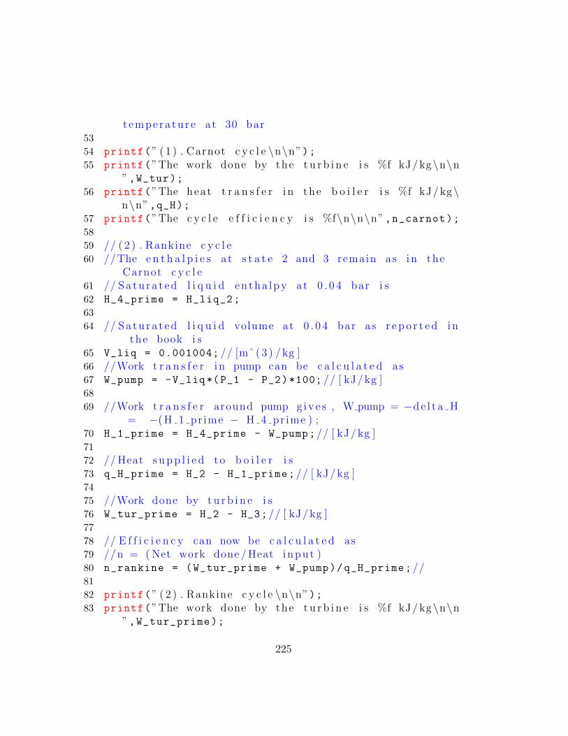
t empera tu re at 30 bar53

54 printf(” ( 1 ) . Carnot c y c l e \n\n”);55 printf(”The work done by the t u r b i n e i s %f kJ/ kg\n\n

”,W_tur);56 printf(”The heat t r a n s f e r i n the b o i l e r i s %f kJ/ kg\

n\n”,q_H);57 printf(”The c y c l e e f f i c i e n c y i s %f\n\n\n”,n_carnot);58

59 // ( 2 ) . Rankine c y c l e60 //The e n t h a l p i e s at s t a t e 2 and 3 remain as i n the

Carnot c y c l e61 // S a t u r a t ed l i q u i d en tha lpy at 0 . 0 4 bar i s62 H_4_prime = H_liq_2;

63

64 // S a t u r a t ed l i q u i d volume at 0 . 0 4 bar as r e p o r t e d i nthe book i s

65 V_liq = 0.001004; // [mˆ ( 3 ) / kg ]66 //Work t r a n s f e r i n pump can be c a l c u l a t e d as67 W_pump = -V_liq*(P_1 - P_2)*100; // [ kJ/ kg ]68

69 //Work t r a n s f e r around pump g i v e s , W pump = −d e l t a H= −( H 1 pr ime − H 4 pr ime ) ;

70 H_1_prime = H_4_prime - W_pump;// [ kJ/ kg ]71

72 // Heat s u p p l i e d to b o i l e r i s73 q_H_prime = H_2 - H_1_prime;// [ kJ/ kg ]74

75 //Work done by t u r b i n e i s76 W_tur_prime = H_2 - H_3;// [ kJ/ kg ]77

78 // E f f i c i e n c y can now be c a l c u l a t e d as79 //n = ( Net work done / Heat input )80 n_rankine = (W_tur_prime + W_pump)/q_H_prime;//81

82 printf(” ( 2 ) . Rankine c y c l e \n\n”);83 printf(”The work done by the t u r b i n e i s %f kJ/ kg\n\n

”,W_tur_prime);

225

84 printf(”The heat t r a n s f e r i n the b o i l e r i s %f kJ/ kg\n\n”,q_H_prime);

85 printf(”The c y c l e e f f i c i e n c y i s %f”,n_rankine);

Scilab code Exa 8.2 Calculation of efficiency of Rankine cycle

1 clear;

2 clc;

3


8 // Given9 T_max = 700+273.15; // [K] − Maximum tempera tu re .10 P_boiler = 10*10^(6);// [ Pa ] − Constant p r e s s u r e i n

the b o i l e r11 P_condenser = 10*10^(3);// [ Pa ] − Constant p r e s s u r e

i n the co nde n s e r12

13 //At s t a t e 2 i . e , a t 700 C and 10 MPa, i t has beenr e p o r t e d i n the book tha t from steam t a b l e

14 S_2 = 7.1687; // [ kJ/kg−K] − Entropy15 H_2 = 3870.5; // [ kJ/ kg ] − Enthalpy16

17 //At s t a t e 3 i . e , a t 700 C and 10 KPa ,18 S_3 = S_2;// [ kJ/kg−K]− Entropy19

20 // For s t u r a t e d steam at 10 kPa , i t has been r e p o r t e di n the book tha t from steam t a b l e

21 S_liq = 0.6493; // [ kJ/kg−K]− Entropy o f s a t u r a t e dl i q u i d

22 S_vap = 8.1502; // [ kJ/kg−K] − Enthalpy o f s a t u r a t e dl i q u i d

23 // T h e r e f o r e steam i s s a t u r a t e d and i t s d r y n e s s

226

f a c t o r can be c a l c u l a t e d as24 x = (S_2 - S_liq)/( S_vap - S_liq);

25

26 //The en tha lpy at s t a t e 3 i s now c a l c u l a t e d . Forsteam at 10 kPa , i t has been r e p o r t e d i n the booktha t from steam t a b l e

27 H_liq = 191.83; // [ kJ/ kg ]28 H_vap = 2584.7; // [ kJ/ kg ]29 // T h e r e f o r e en tha lpy at s t a t e 3 i s30 H_3 = H_liq *(1-x) + H_vap*x;// [ kJ/ kg ]31

32 //Work done by the t u r b i n e33 W_tur = -(H_3 - H_2);// [ kJ/ kg ]34

35 //Now we have to c a l c u l a t e work input to the pump36 // S t a t e 4 : S a t u r a t ed l i q u i d at 10 kPa37 // S t a t e 4 : Compressed l i q u i d at 10 MPa38 // S i n c e volume o f l i q u i d does not g e t a f f e c t e d by

p r e s s u r e we take volume o f s a t u r a t e d l i q u i d at 10kPa ,

39 V_liq = 0.001010; // [mˆ ( 3 ) / kg ]40

41 //Work t r a n s f e r i n the pump i s42 W_pump = -V_liq*( P_boiler - P_condenser)*10^( -3);// [

kJ/ kg ]43

44 // Energy b a l a n c e around pump g i v e s , W pump = −d e l t a H = −(H 1 − H 4 )

45 H_4 = H_liq;// Enthalpy at s t a t e 4 ( s a t u r a t e d l i q u i dat 10 kPa )

46 H_1 = H_4 - W_pump;// [ kJ/ kg ]47

48 // Heat s u p p l i e d to b o i l e r i s49 q_H = H_2 - H_1;// [ kJ/ kg ]50

51 // E f f i c i e n c y can now be c a l c u l a t e d as52 //n = ( Net work done / Heat input )53 n_rankine = (W_tur + W_pump)/q_H;

227

54

55 printf(”The e f f i c i e n c y o f the Rankine c y c l e i s foundto be %f”,n_rankine);

56

57 //Now l e t us de t e rmine the e f f i c i e n c y o f Carnotc y c l e . The maximun tempera tu r e i s 700 C andminimum tempera tu r e i s tha t o f s a t u r a t e d steam at

10 kPa ,58 T_min = 45.81 + 273.15; // [K] − From steam t a b l e as

r e p o r t e d i n the book59 n_carnot = 1-(T_min/T_max);

60 // Note tha t the e f f i c i e n c y o f Rankine c y c l e i s l e s sthan tha t o f c a r n o t c y c l e .

Scilab code Exa 8.3 Calculatrion of COP of carnot refrigerator and heatrejected

1 clear;

2 clc;

3


8 // Given9 W = 1.1; // [kW] − Work done per ton o f r e f r i g e r a t i o n10 // 1 ton r e f r i g e r a t i o n = 3 . 5 1 7 kW, t h e r e f o r e11 H = 3.517; // [kW] − Heat absorbed12 T_low = -30 + 273.15; // [K] − Low tempera tu r e

ma inta ined13

14 //COP can be c a l c u l a t e d as15 //COP = ( Heat absorbed /Work done )16 COP = H/W;

17

228

18 // For r e v e r s e d c a r n o t c y c l e , COP = T low /( T high −T low ) . S o l v i n g t h i s we ge t

19 T_high = (T_low/COP) + T_low;// [K] − Highert empera tu re

20

21 // Heat r e j e c t e d i s22 H_rej = W + H;// [kW] ;23

24 printf(”The COP i s %f\n\n”,COP);25 printf(”The h i g h e r t empera tu r e o f the c y c l e i s %f K\

n\n”,T_high);26 printf(”The heat r e j e c t e d per ton o f r e f r i g e r a t i o n

i s %f kW\n\n”,H_rej);

Scilab code Exa 8.4 Calculation of minimum power required

1 clear;

2 clc;

3


8 // Given9 T_high = 20 + 273.15; // [K] − High tempera tu r e10 T_low = 0 + 273.15; // [K] − Low tempera tu r e11 Q_H = 10; // [kW] − Heat s u p p l i e d12

13 // I f ’Q H ’ i s the r a t e at which heat i s taken froms u r r o u n d i n g and ’W’ i s the r a t e at which work i sdone , then

14 // Q H = W + Q L15 // (Q H/Q L ) = ( T high / T low )16 // Also f o r a r e v e r s i b l e c y c l e , (Q H/Q L ) = 1 + (W/

Q L ) . S o l v i n g we get ,

229

17 Q_L = (T_low/T_high)*Q_H;// [kW]18 W = (Q_H - Q_L) ;// [kW]19

20 printf(”The minimum power r e q u i r e d i s %f kW”,W);

Scilab code Exa 8.5 Determination of COP and power required

1 clear;

2 clc;

3


8 // Given9 T_high = 40 + 273.15; // [K] − High tempera tu r e10 T_low = -20 + 273.15; // [K] − Low tempera tu r e11 C = 10; // [ t on s o f r e f r i g e r a t i o n ] − Capac i ty12 // 1 ton r e f r i g e r a t i o n = 3 . 5 1 7 kW, t h e r e f o r e13 H = C*3.517; // [kW] − Heat absorbed14

15 // For r e v e r s e d c a r n o t c y c l e , COP = T low /( T high −T low )

16 COP = T_low /( T_high - T_low);

17

18 // COP = ( R e f r i g e r a t i n g e f f e c t ) /( Work input ) ,t h e r e f o r e power r e q u i r e d i s g i v e n by

19 P = (H/COP);// [kW]20

21 printf(”The COP i s %f\n\n”,COP);22 printf(”The power r e q u i r e d i s %f kW”,P);

Scilab code Exa 8.6 Determination of maximum refrigeration effect

230

1 clear;

2 clc;

3


8 // Given9 COP = 4; // C o e f f i c i e n t o f pe r f o rmance10 P = 10; // [kW] − Work done on the c y c l e11

12 // For r e v e r s e d c a r n o t c y c l e , COP = T low /( T high −T low )

13 // r a t i o = ( T high / T low ) , t h e r e f o r e14 ratio = -1/(COP + 1);

15

16 // R e f r i g e r a t i n g e f f e c t = (COP) ∗Work input ,t h e r e f o r e r e f r i g e r a t i o n i s g i v e n by

17 H = COP*P;// [kW]18

19 //Maximum r e f r i g e a r a t i o n i n ton s i s g i v e n by20 H_max = (H/3.517);

21

22 printf(”The maximum r e f r i g e r a t i o n v a l u e i s %f ton ”,H_max);

Scilab code Exa 8.7 Determination of refrigeration effect power consumedand COP of refrigerator

1 clear;

2 clc;

3

4 // Example − 8 . 75 // Page number − 2926 printf(” Example − 8 . 7 and Page number − 292\n\n”);

231

7

8 // Given9 m = 0.6; // [ kg / s ] − mass f l o w r a t e10 T_low = -20+273.15; // [K] − Temperature at which

vapour e n t e r s the compre s so r11 T_high = 30+273.15; // [K] − Temperature at which

vapour l e a v e s the co nden s e r12

13 //From s a t u r a t e d r e f r i g e r a t i o n −12 t a b l e s we get , a t−20 C

14 H_1 = 178.74; // [ kJ/ kg ] − ( H 1 = H vap )15 P_1 = 0.15093; // [MPa] − ( P 1 = P sa t )16 P_4 = P_1;

17 S_1 = 0.7087; // [ kJ/kg−K] − ( S 1 = S vap )18 S_2 = S_1;

19

20 //At 30 C21 P_2 = 0.7449; // [MPa] − ( P 2 = P sa t )22 P_3 = P_2;

23 H_3 = 64.59; // [ kJ/ kg ] − ( H 3 = H l i q )24 H_4 = H_3;

25 S_3 = 0.24; // [ kJ/kg−K] − ( S 3 = S l i q )26

27 // I t i s assumed tha t p r e s s s u r e drop i n thee v a p o r a t o r and co nde n s e r a r e n e g l i g i b l e . The heat

t r a n s f e r r a t e i n the e v a p o r a t o r i s28 Q_L = m*(H_1 - H_4);

29

30 printf(”The heat t r a n s f e r r a t e i n the e v a p o r a t o r i s%f kW\n\n”,Q_L);

31

32 //At s t a t e 2 (P = 0 . 7 4 4 9 MPa and S = 0 . 7 0 8 7 kJ/kg−K)and l o o k i n g i n the s u p e r h e a t e d t a b l e s we have toc a l c u l a t e the en tha lpy at s t a t e 2

33

34 //At P = 0 . 7 MPa and S = 0 . 6 9 1 7 kJ/kg−K,35 H_11 = 200.46; // [ kJ/ kg ]36

232


40 // Thus at P = 0 . 7 MPa and S = 0 . 7 0 8 7 kJ/kg−K,en tha lpy i s g i v e n by

41 H_13 = ((S_2 -0.6917) /(0.7153 - 0.6917))*(H_12 -

H_11) + H_11;// [ kJ/ kg ]42



49 // Thus at P = 0 . 8 MPa and S = 0 . 7 0 8 7 kJ/kg−K,en tha lpy i s g i v e n by

50 H_23 = ((S_2 -0.7021) /(0.7253 - 0.7021))*(H_22 -

H_21) + H_21;// [ kJ/ kg ]51

52 //At P = 0 . 7 4 4 9 MPa, S = 0 . 7 0 8 7 kJ/kg−K, theen tha lpy i s

53 H_2 = ((0.7449 - 0.7) /(0.8 - 0.7))*(H_23 - H_13) +

H_13;// [ kJ/ kg ]54

55 // Power consumed by the compre s so r i s56 W_comp = m*(H_2 - H_1);// [kW]57

58 printf(”The power consumed by the compre s so r i s %fkW\n\n”,W_comp);

59

60 // Heat removed i n e v a p o r a t o r / work done on compre s so r61 COP_R = Q_L/W_comp;

62

63 printf(”The COP the r e f r i g e r a t o r i s %f kW\n\n”,COP_R);

64

65

66 //At −20 C, s a t u r a t e d c o n d i t i o n s

233

67 H_liq = 17.82; // [ kJ/ kg ]68 H_vap = 178.74; // [ kJ/ kg ]69 x_4 = (H_4 - H_liq)/(H_vap - H_liq);

70

71 printf(”The d r y n e s s f a c t o r o f r e f r i g e r a n t a f t e r theexpans i on v a l v e i s %f\n\n”,x_4);

72

73 //The heat t r a n s f e r r a t e i n the co nde n s e r i s74 Q_H = m*(H_3 - H_2);// [kW]75

76 printf(”The heat t r a n s f e r r a t e i n the c ond en s e r i s%f kW\n\n”,Q_H);

77

78 // I f the c y c l e would have worked as a pump then ,79 //COP HP = ( Heat s u p p l i e d from con den s e r /Work done

on compre s so r )80 COP_HP = (-Q_H)/W_comp;

81

82 printf(”The COP i f c y c l e would work as a heat pumpi s %f kW\n\n”,COP_HP);

83

84 // I f the c y c l e would have been a r e v e r s e d Carnotc y c l e then

85 COP_C = T_low /( T_high - T_low);

86

87 printf(”The COP i f c y c l e would run as r e v e r s e dCarnot c y c l e i s %f kW\n\n”,COP_C);

Scilab code Exa 8.8 Calculation of amount of air

1 clear;

2 clc;

3


234

6 printf(” Example − 8 . 8 and Page number − 300\n\n”);7

8 // Given9 //From compre s so r to the expans i on v a l v e the

p r e s s u r e i s 200 bar and from expans i on v a l v e tothe i n l e t o f compre s so r the p r e s s u r e i s 1 bar .

10 // Po int 5 i s s a t u r a t e d l i q u i d at 1 bar and p o i n t 6i s s a t u r a t e d vapour at 1 bar

11

12 // I t has been r e p o r t e d i n the book tha t at s t a t e 1(310 K, 1 bar )

13 H_1 = 310.38; // [ kJ/ kg ]14 //At s t a t e 2 (310 K, 200 bar )15 H_2 = 277.7; // [ kJ/ kg ]16 //At s t a t e 5 (1 bar , s a t u r a t e d l i q u i d )17 H_5 = -122.6; // [ kJ/ kg ]18 //At s t a t e 6 (1 bar , s a t u r a t e d vapur )19 H_6 = 77.8; // [ kJ/ kg ]20

21 //The en tha lpy at p o i n t 3 i s same at p o i n t 4 as theexpans i on i s i s e n t h a l p i c

22

23 //The mass condensed i s 1 kg and t h e r e f o r e m 1 = m+6+ 1

24

25 // Enthalpy b a l a n c e around heat exchange r26 //m 2∗H 2 + m 2∗H 6 = m 3∗H 3 + m 7∗H 727

28 // Enthalpy b a l a n c e around s e p a r a t o r29 //m 4∗H 4 = m 5∗H 5 + m 6∗H 630 // I t can be s e en tha t m 1 = m 2 = m 3 = m 431 // and m 6 = m 7 = m 1 − 132

33 // S u b s t i t u t i n g the v a l u e s f o r en tha lpy b a l a n c earound heat exchange r we get ,

34 //m 1∗H 2 + ( m 1 − 1) ∗ ( H 6 ) = m 1∗H 3 + ( m 1 − 1) ∗H 1

35 // and s u b s t i t u t i n g the v a l u e s f o r en tha lpy b a l a n c e

235

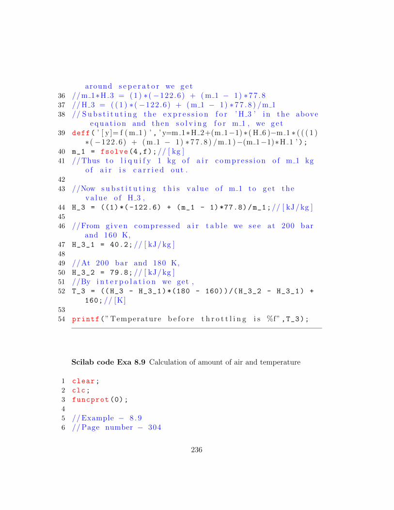
around s e p e r a t o r we g e t36 //m 1∗H 3 = ( 1 ) ∗ ( −122 .6) + ( m 1 − 1) ∗7 7 . 837 // H 3 = ( ( 1 ) ∗ ( −122 .6) + ( m 1 − 1) ∗ 7 7 . 8 ) /m 138 // S u b s t i t u t i n g the e x p r e s s i o n f o r ’ H 3 ’ i n the above

e q u a t i o n and then s o l v i n g f o r m 1 , we ge t39 deff( ’ [ y ]= f ( m 1 ) ’ , ’ y=m 1∗H 2+(m 1−1) ∗ ( H 6 )−m 1 ∗ ( ( ( 1 )

∗ ( −122 .6) + ( m 1 − 1) ∗ 7 7 . 8 ) /m 1 )−(m 1−1)∗H 1 ’ );40 m_1 = fsolve(4,f);// [ kg ]41 // Thus to l i q u i f y 1 kg o f a i r c ompre s s i on o f m 1 kg

o f a i r i s c a r r i e d out .42

43 //Now s u b s t i t u t i n g t h i s v a l u e o f m 1 to g e t thev a l u e o f H 3 ,

44 H_3 = ((1) *( -122.6) + (m_1 - 1) *77.8)/m_1;// [ kJ/ kg ]45

46 //From g i v e n compressed a i r t a b l e we s e e at 200 barand 160 K,

47 H_3_1 = 40.2; // [ kJ/ kg ]48

49 //At 200 bar and 180 K,50 H_3_2 = 79.8; // [ kJ/ kg ]51 //By i n t e r p o l a t i o n we get ,52 T_3 = ((H_3 - H_3_1)*(180 - 160))/( H_3_2 - H_3_1) +

160; // [K]53

54 printf(” Temperature b e f o r e t h r o t t l i n g i s %f”,T_3);

Scilab code Exa 8.9 Calculation of amount of air and temperature

1 clear;

2 clc;

3 funcprot (0);

4


236

7 printf(” Example − 8 . 9 and Page number − 304\n\n”);8

9 // Given10 //At 1 bar , 310 K11 H_1 = 310.38; // [ kJ/ kg ]12 //At 200 bar , 310 K13 H_2 = 277.7; // [ kJ/ kg ]14 //At 1 bar , S a t u r a t e d l i q u i d15 H_7 = -122.6; // [ kJ/ kg ]16 //At 1 bar , S a t u r a t e d vapour17 H_8 = 77.8; // [ kJ/ kg ]18 //At 200 bar , 200 K19 H_3 = 117.6; // [ kJ/ kg ]20 //At 1 bar , 100 K21 H_11 = 98.3; // [ kJ/ kg ]22

23 // ( 1 )24 // For 1 kg o f l i q u i d a i r obta ined , the o v e r a l l

en tha lpy b a l a n c e i s25 //m 2∗H 2 = W − 1 2 2 . 6 + ( m 2 − 1) ∗H 126 //W = − 0 . 8∗m 2 ∗ ( H 11 − H 3 )27 // O v e r a l l en tha lpy b a l a n c e e q u a t i o n becomes28 // H 2∗m 2 = 1 5 . 4 4∗m 2 − H 7 + ( m 2 − 1) ∗H 1 , s o l v i n g29 m_2_prime = (H_7 - H_1)/(H_2 - 15.44 - H_1);

30

31 printf(”The number o f k i l o g r a m s o f a i r compressedper kg o f l i q u i d a i r produced i s %f kg\n\n”,m_2_prime);

32

33 // ( 2 )34 // Enthalpy b a l a n c e around s e p a r a t o r i s35 // 0 . 2∗m 2∗H 5 = −H 7 + ( 0 . 2 ∗m 2 − 1) ∗H 8 , s o l v i n g36 m_2 = m_2_prime;

37 H_5_prime = ((0.2*m_2 -1)*H_8 - H_7)/(0.2* m_2);

38

39 //At p o i n t 5 , P = 200 bar and en tha lpy i s40 H_5_1 = -33.53; // [ kJ/ kg ]41 //From compressed a i r t a b l e s at 200 bar and 140 K,

237

42 H_5_2 = 0.2; // [ kJ/ kg ]43 //At 200 bar and 120 K,44 H_5_3 = -38.0; // [ kJ/ kg ]45 // S o l v i n g by i n t e r p o l a t i o n we ge t46 T_5 = ((H_5_1 - H_5_3)*(140 - 120))/( H_5_2 - H_5_3)

+ 120; // [K]47

48 printf(”The tempera tu r e o f a i r b e f o r e t h r o t t l i n g i s%f K\n\n”,T_5);

49

50 // ( 3 )51 // During mix ing o f s t r eams 8 and 11 to produce

stream 9 , the en tha lpy b a l a n c e i s52 // ( 0 . 2 ∗m 2 − 1) ∗H 8 + 0 . 8∗m 2∗H 11 = ( m 2 − 1) ∗H 9 ,

S o l v i n g f o r H 953

54 H_9_prime = ((0.2*m_2 -1)*H_8 +0.8* m_2*H_11)/(m_2 - 1)

;

55

56 //From g i v e n compressed a i r t a b l e s at 1 bar and 100K,

57 H_9_1 = H_11;

58 //At 1 bar and 90 K59 H_9_2 = 87.9; // [ kJ/ kg ]60 // S o l v i n g by i n t e r p o l a t i o n we ge t61 T_9 = (( H_9_prime - H_9_2)*(100 - 90))/(H_9_1 -

H_9_2) + 90; // [K]62

63 printf(”The tempera tu r e o f s t ream e n t e r i n g secondheat exchange r i s %f K\n\n”,T_9);

64

65 // ( 4 )66 // Enthalpy b a l a n c e around f i r s t heat exchange r i s67 // H 2∗m 2 + ( m 2 − 1) ∗H 10 = H 3∗m−2 + (m−2 − 1) ∗H 1

, s o l v i n g f o r H 1068

69 H_10_prime = ((m_2 - 1)*H_1 + H_3*m_2 - H_2*m_2)/(

m_2 - 1);

238

70


72 H_10_1 = 139.1; // [ kJ/ kg ]73 //At 1 bar and 120 K74 H_10_2 = 118.8; // [ kJ/ kg ]75 // S o l v i n g by i n t e r p o l a t i o n we ge t76 T_10 = (( H_10_prime - H_10_2)*(140 - 120))/( H_10_1 -

H_10_2) + 120; // [K]77

78 printf(”The tempera tu r e o f s t ream e x i t i n g secondheat exchange r i s %f K\n\n”,T_10);

Scilab code Exa 8.10 Determination of temperature of air

1 clear;

2 clc;

3 funcprot (0);

4


9 // Given10 P_high = 40; // [ bar ]11 P_low = 5; // [ bar ]12 m_1 = 0.5; // [ kg / s ] − Rate o f mass moving through the

expander13 m_2 = 0.1; // [ kg / s ] − Rate o f mass o f vapour mixing

with a i r14 e = 0.7; // E f f i c i e n c y15

16 //At s t a t e 3 , ( 4 0 bar and 200 K) , en tha lpy and ent ropyi s g i v e n by

17 H_3 = 179.7; // [ kJ/ kg ]

239

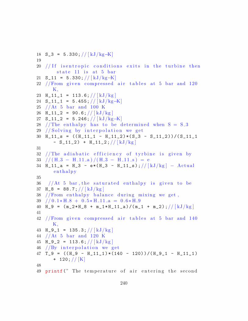
18 S_3 = 5.330; // [ kJ/kg−K]19

20 // I f i s e n t r o p i c c o n d i t i o n s e x i t s i n the t u r b i n e thens t a t e 11 i s at 5 bar

21 S_11 = 5.330; // [ kJ/kg−K]22 //From g i v e n compressed a i r t a b l e s at 5 bar and 120

K,23 H_11_1 = 113.6; // [ kJ/ kg ]24 S_11_1 = 5.455; // [ kJ/kg−K]25 //At 5 bar and 100 K26 H_11_2 = 90.6; // [ kJ/ kg ]27 S_11_2 = 5.246; // [ kJ/kg−K]28 //The en tha lpy has to be dete rmined when S = S 329 // S o l v i n g by i n t e r p o l a t i o n we ge t30 H_11_s = (( H_11_1 - H_11_2)*(S_3 - S_11_2))/( S_11_1

- S_11_2) + H_11_2;// [ kJ/ kg ]31

32 //The a d i a b a t i c e f f i c i e n c y o f t y r b i n e i s g i v e n by33 // ( H 3 − H 11 a ) /( H 3 − H 11 s ) = e34 H_11_a = H_3 - e*(H_3 - H_11_s);// [ kJ/ kg ] − Actua l

en tha lpy35

36 //At 5 bar , the s a t u r a t e d en tha lpy i s g i v e n to be37 H_8 = 88.7; // [ kJ/ kg ]38 //From entha lpy b a l a n c e dur ing mixing we get ,39 // 0 . 1∗H 8 + 0 . 5∗ H 11 a = 0 . 6∗H 940 H_9 = (m_2*H_8 + m_1*H_11_a)/(m_1 + m_2);// [ kJ/ kg ]41


43 H_9_1 = 135.3; // [ kJ/ kg ]44 //At 5 bar and 120 K45 H_9_2 = 113.6; // [ kJ/ kg ]46 //By i n t e r p o l a t i o n we g e t47 T_9 = ((H_9 - H_11_1)*(140 - 120))/( H_9_1 - H_11_1)

+ 120; // [K]48

49 printf(” The tempera tu r e o f a i r e n t e r i n g the second

240

heat exchange r i s %f K\n\n”,T_9);

241

Chapter 10

Residual Properties byEquations of State

Scilab code Exa 10.1 Determination of expression for residual enthalpyinternal energy and Gibbs free energy

1 clear;

2 clc;

3

4 // Example − 1 0 . 15 // Page number − 3236 printf(” Example − 1 0 . 1 and Page number − 323\n\n”);7

8 // This problem i n v o l v e s p rov ing a r e l a t i o n i n whichno mathemat i ca l components a r e i n v o l v e d .

9 // For prove r e f e r to t h i s example 1 0 . 1 on pagenumber 323 o f the book .

10 printf(” This problem i n v o l v e s p rov ing a r e l a t i o n i nwhich no mathemat i ca l components a r e i n v o l v e d . \ n\n”);

11 printf(” For prove r e f e r to t h i s example 1 0 . 1 on pagenumber 323 o f the book . ”)

242

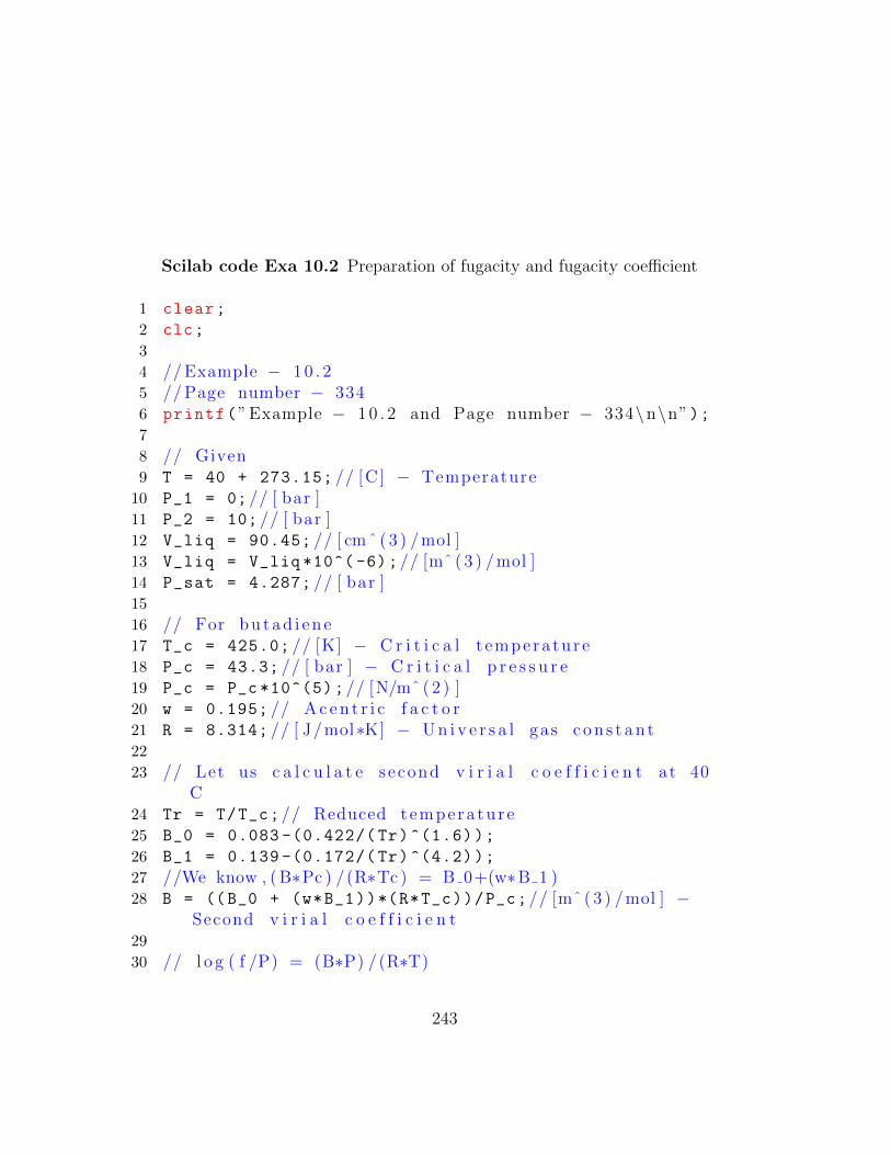
Scilab code Exa 10.2 Preparation of fugacity and fugacity coefficient

1 clear;

2 clc;

3


8 // Given9 T = 40 + 273.15; // [C ] − Temperature10 P_1 = 0; // [ bar ]11 P_2 = 10; // [ bar ]12 V_liq = 90.45; // [ cm ˆ ( 3 ) /mol ]13 V_liq = V_liq *10^( -6);// [mˆ ( 3 ) /mol ]14 P_sat = 4.287; // [ bar ]15

16 // For bu t a d i e n e17 T_c = 425.0; // [K] − C r i t i c a l t empera tu r e18 P_c = 43.3; // [ bar ] − C r i t i c a l p r e s s u r e19 P_c = P_c *10^(5);// [N/mˆ ( 2 ) ]20 w = 0.195; // A c e n t r i c f a c t o r21 R = 8.314; // [ J/mol∗K] − U n i v e r s a l gas c o n s t a n t22

23 // Let us c a l c u l a t e second v i r i a l c o e f f i c i e n t at 40C

24 Tr = T/T_c;// Reduced tempera tu r e25 B_0 = 0.083 -(0.422/( Tr)^(1.6));

26 B_1 = 0.139 -(0.172/( Tr)^(4.2));

27 //We know , ( B∗Pc ) /(R∗Tc ) = B 0+(w∗B 1 )28 B = ((B_0 + (w*B_1))*(R*T_c))/P_c;// [mˆ ( 3 ) /mol ] −

Second v i r i a l c o e f f i c i e n t29

30 // l o g ( f /P) = (B∗P) /(R∗T)

243

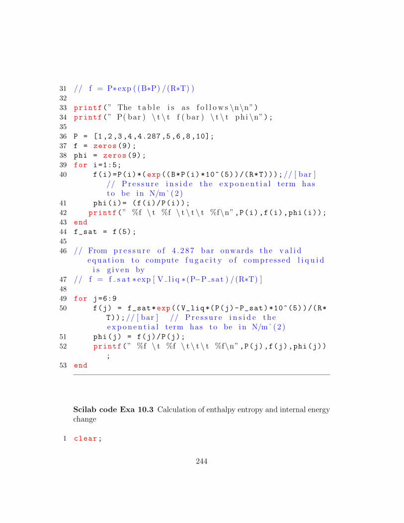
31 // f = P∗ exp ( (B∗P) /(R∗T) )32

33 printf(” The t a b l e i s as f o l l o w s \n\n”)34 printf(” P( bar ) \ t \ t f ( bar ) \ t \ t ph i \n”);35

36 P = [1,2,3,4,4.287,5,6,8,10];

37 f = zeros (9);

38 phi = zeros (9);

39 for i=1:5;

40 f(i)=P(i)*(exp((B*P(i)*10^(5))/(R*T)));// [ bar ]// P r e s s u r e i n s i d e the e x p o n e n t i a l term hasto be i n N/mˆ ( 2 )

41 phi(i)= (f(i)/P(i));

42 printf(” %f \ t %f \ t \ t \ t %f\n”,P(i),f(i),phi(i));43 end

44 f_sat = f(5);

45

46 // From p r e s s u r e o f 4 . 2 8 7 bar onwards the v a l i de q u a t i o n to compute f u g a c i t y o f compressed l i q u i d

i s g i v e n by47 // f = f s a t ∗ exp [ V l i q ∗ (P−P sa t ) /(R∗T) ]48

49 for j=6:9

50 f(j) = f_sat*exp(( V_liq*(P(j)-P_sat)*10^(5))/(R*

T));// [ bar ] // P r e s s u r e i n s i d e thee x p o n e n t i a l term has to be i n N/mˆ ( 2 )

51 phi(j) = f(j)/P(j);

52 printf(” %f \ t %f \ t \ t \ t %f\n”,P(j),f(j),phi(j));

53 end

Scilab code Exa 10.3 Calculation of enthalpy entropy and internal energychange

1 clear;

244

2 clc;

3


8 // Given9 n = 100; // [ mol ] − No o f moles10 T_1 = 600; // [K] − I n i t i a l t empera tu re11 T_2 = 300; // [K] − F i n a l t empera tu r e12 P_1 = 10; // [ atm ] − I n i t i a l p r e s s u r e13 P_1 = P_1 *101325; // [ Pa ]14 P_2 = 5; // [ atm ] − F i n a l p r e s s s u r e15 P_2 = P_2 *101325; // [ Pa ]16 Tc = 369.8; // [K] − C r i t i c a l t empera tu r e17 Pc = 42.48; // [ bar ] − C r i t i c a l p r e s s u r e18 Pc = Pc *10^(5);// [ Pa ]19 w = 0.152;


22 // At 600 K23 Tr = T_1/Tc;// Reduced tempera tu r e24 B_0 = 0.083 -(0.422/( Tr)^(1.6));

25 B_1 = 0.139 -(0.172/( Tr)^(4.2));

26 //We know , ( B∗Pc ) /(R∗Tc ) = B 0 + (w∗B 1 )27 B = ((B_0 + (w*B_1))*(R*Tc))/Pc;// [mˆ ( 3 ) /mol ] −

Second v i r i a l c o e f f i c i e n t28 dB0_dT = 0.422*1.6* Tc ^(1.6)*T_1 ^( -2.6);// ( dB 0 /dT)29 dB1_dT = 0.172*4.2* Tc ^(4.2)*T_1 ^( -5.2);// ( dB 1 /dT)30 dB_dT = ((R*Tc)/(Pc))*( dB0_dT + w*dB1_dT);// dB/dT31

32 // Now l e t us c a l c u l a t e B and dB/dT at 300 K33 Tr_prime = T_2/Tc;// Reduced tempera tu r e34 B_0_prime = 0.083 -(0.422/( Tr_prime)^(1.6));

35 B_1_prime = 0.139 -(0.172/( Tr_prime)^(4.2));

36 //We know , ( B∗Pc ) /(R∗Tc ) = B 0 + (w∗B 1 )37 B_prime = (( B_0_prime + (w*B_1_prime))*(R*Tc))/Pc;//

[mˆ ( 3 ) /mol ] − Second v i r i a l c o e f f i c i e n t

245

38 dB0_dT_prime = 0.422*1.6* Tc ^(1.6)*T_2 ^( -2.6);// (dB 0 /dT)

39 dB1_dT_prime = 0.172*4.2* Tc ^(4.2)*T_2 ^( -5.2);// (dB 1 /dT)

40 dB_dT_prime = ((R*Tc)/(Pc))*( dB0_dT_prime + w*

dB1_dT_prime);// dB/dT41

42 // The change i n en tha lpy f o r i d e a l gas i s g i v e n by43 delta_H_ig = integrate( ’ −0.966+7.279∗10ˆ(−2) ∗T

−3.755∗10ˆ(−5) ∗Tˆ ( 2 ) +7.58∗10ˆ(−9) ∗Tˆ ( 3 ) ’ , ’T ’ ,T_1 ,T_2);// [ c a l /mol ]

44 delta_H_ig = delta_H_ig *4.184; // [ J/mol ]45

46 // We know tha t d e l t a H i g = d e l t a U i g + R∗ d e l t a T .T h e r e f o r e change i n i n t e r n a l ene rgy i s g i v e n by

47 delta_U_ig = delta_H_ig - R*(T_2 - T_1);// [ J/mol ]48

49 // The change i n ent ropy o f i d e a l gas i s g i v e n by50 // d e l t a S i g = i n t e g r a t e ( ’ Cp 0 /T’ , ’ T’ , T 1 , T 2 ) − R∗

l o g ( P 2 / P 1 ) ;51 delta_S_ig = integrate( ’ (−0.966+7.279∗10ˆ(−2) ∗T

−3.755∗10ˆ(−5) ∗Tˆ ( 2 ) +7.58∗10ˆ(−9) ∗Tˆ ( 3 ) ) /T ’ , ’T ’ ,T_1 ,T_2)*4.184 - R*log(P_2/P_1);// [ J/mol−K]

52

53 // Now l e t us c a l c u l a t e the change i n en tha lpy o fgas . We know tha t

54 // d e l t a H = d e l t a H i g + de l ta H R55 // de l ta H R = H 2 R − H 1 R56 H_2_R = B_prime*P_2 - P_2*T_2*dB_dT_prime;// [ J/mol ]57 H_1_R = B*P_1 - P_1*T_1*dB_dT;// [ J/mol ]58 delta_H_R = H_2_R - H_1_R;// [ J/mol ]59 delta_H = delta_H_ig + delta_H_R;// [ J/mol ]60

61 // Let us c a l c u l a t e the r e s i d u a l ent ropy o f gas62 S_2_R = -P_2*dB_dT_prime;// [ J/mol−K]63 S_1_R = -P_1*dB_dT;// [ J/mol−K]64 delta_S = delta_S_ig + (S_2_R - S_1_R);// [ J/mol−K]65

246

66 // Let us c a l c u l a t e the r e s i d u a l i n t e r n a l ene rgy o fgas

67 U_2_R = -P_2*T_2*dB_dT_prime;// [ J/mol−K]68 U_1_R = -P_1*T_1*dB_dT;// [ J/mol−K]69 delta_U = delta_U_ig + (U_2_R - U_1_R);// [ J/mol−K]70

71 // For 100 mol sample ,72 delta_H_ig = delta_H_ig*n*10^( -3);// [ kJ/mol ]73 delta_H = delta_H*n*10^( -3);// [ kJ/mol ]74

75 delta_U_ig = delta_U_ig*n*10^( -3);// [ kJ/mol ]76 delta_U = delta_U*n*10^( -3);// [ kJ/mol ]77

78 delta_S_ig = delta_S_ig*n*10^( -3);// [ kJ/mol ]79 delta_S = delta_S*n*10^( -3);// [ kJ/mol ]80

81 printf(” The v a l u e o f d e l t a H = %f kJ/mol\n”,delta_H);

82 printf(” The v a l u e o f d e l t a H i g ( i d e a l gas )= %f kJ/mol\n\n”,delta_H_ig);

83 printf(” The v a l u e o f d e l t a U = %f kJ/mol\n”,delta_U);

84 printf(” The v a l u e o f d e l t a U i g ( i d e a l gas ) = %f kJ/mol\n\n”,delta_U_ig);

85 printf(” The v a l u e o f d e l t a S = %f kJ/mol\n”,delta_S);

86 printf(” The v a l u e o f d e l t a S i g ( i d e a l gas ) = %f kJ/mol\n\n”,delta_S_ig);

Scilab code Exa 10.4 Calculation of molar heat capacity

1 clear;

2 clc;

3

4 // Example − 1 0 . 4

247

5 // Page number − 3376 printf(” Example − 1 0 . 4 and Page number − 337\n\n”);7

8 // Given9 T = 35 + 273.15; // [K] − Temperature10 P = 10; // [ atm ] − P r e s s u r e11 P = P*101325; // [ Pa ]12 // Methane obeys the e q u a t i o n o f s t a t e13 // Z = 1 + (P∗B) /(R∗T)14

15 // At 35 C,16 B = -50; // [ cm ˆ ( 3 ) /mol ]17 dB_dT = 1.0; // [ cm ˆ ( 3 ) /mol−K] − dB/dT18 dB_dT = dB_dT *10^( -6);// [mˆ ( 3 ) /mol−K]19 d2B_dT2 = -0.01; // [ cm ˆ ( 3 ) /mol−Kˆ ( 2 ) ] − d ˆ2(B) /d (Tˆ2)20 d2B_dT2 = d2B_dT2 *10^( -6);// [mˆ ( 3 ) /mol−Kˆ ( 2 ) ]21

22 // I d e a l gas molar heat c a p a c i t y o f methane i s g i v e nby

23 // Cp 0 = 4 . 7 5 + 1.2∗10ˆ( −2) ∗T + 0.303∗10ˆ( −5) ∗Tˆ ( 2 )− 2 .63∗10ˆ( −9) ∗Tˆ ( 3 )

24

25 // The molar heat c a p a c i t y i s g i v e n by26 // Cp = Cp 0 + Cp R27 // For v i r i a l gas e q u a t i o n o f s t a t e28 Cp_R = -P*T*d2B_dT2;// [ J/mol−K]29

30 // thus heat c a p a c i t y i s g i v e n by31 // Cp = a + b∗T + c ∗Tˆ ( 2 ) + d∗Tˆ ( 3 ) − P∗T∗d2B dT232 // Put t ing the va lue s , we ge t33 Cp = (4.75 + 1.2*10^( -2)*T + 0.303*10^( -5)*T^(2) -

2.63*10^( -9)*T^(3))*4.184 - P*T*d2B_dT2;// [ J/mol−K]

34

35 printf(” The molar heat c a p a c i t y o f methane i s %f J/mol−K\n”,Cp);

248

Scilab code Exa 10.5 Calculation of final temperature after expansion

1 clear;

2 clc;

3


8 // Given9 T_1 = 360; // [K] − I n i t i a l t empera tu re10 P_1 = 10; // [ bar ] − I n i t i a l p r e s s u r e11 P_1 = P_1 *10^(5);// [ Pa ]12 Tc = 408.1; // [K] − C r i t i c a l t empera tu r e13 Pc = 36.48; // [ bar ] − C r i t i c a l p r e s s u r e14 Pc = Pc *10^(5);// [ Pa ]15 w = 0.181;

16 R = 8.314; // [ J/mol∗K] − U n i v e r s a l gas c o n s t a n t17 Cv_0 = 106.0; // [ J/mol−K]18

19 // At 360 K20 Tr = T_1/Tc;// Reduced tempera tu r e21 B_0 = 0.083 -(0.422/( Tr)^(1.6));

22 B_1 = 0.139 -(0.172/( Tr)^(4.2));


Second v i r i a l c o e f f i c i e n t25 dB0_dT = 0.422*1.6* Tc ^(1.6)*T_1 ^( -2.6);// ( dB 0 /dT)26 dB1_dT = 0.172*4.2* Tc ^(4.2)*T_1 ^( -5.2);// ( dB 1 /dT)27 dB_dT = ((R*Tc)/(Pc))*( dB0_dT + w*dB1_dT);// dB/dT28

29 // S i n c e system i s a d i a b a t i c t h e r e f o r e no heatexchange w i l l t ake p l a c e , q = 0

30 // and expans i on t a k e s p l a c e i n t o vacuum , t h r e f o r e W

249

= 031 // From f i r s t law d e l t a U = 0 . I f the gas would have

f o l l o w e d i d e a l gas e q u a t i o n o f s t a t e the f i n a lt empera tu re would have been the same as i n i t i a las d e l t a U = 0

32 // But f o r r e a l g a s e s33 // d e l t a U = d e l t a U i g + de l ta U R34 // d e l t a U = d e l t a U i g + U 2 R − U 1 R35 // For e q u a t i o n o f s t a t e Z = 1 + (B∗P) /(R∗T)36 // V = B + (R∗T) /P37 // U R = −P∗T∗ (dB/dT)38

39 // d e l t a U i g = Cv 0 ∗ ( T 2 − T 1 )40 // d e l t a U = Cv 0 ∗ ( T 2 − T 1 ) − P 2∗T 2 ∗ (dB/dT) 2 +

P 1∗T 1 ∗ (dB/dT) 141

42 // At s t a t e 143 V_1 = B + (R*T_1)/P_1;// [mˆ ( 3 ) /mol ] − Molar volume44 // At s t a t e 145 V_2 = 10*V_1;// [mˆ ( 3 ) /mol ] − Molar volume46

47 // From the e q u a t i o n d e l t a U = 048 // Cv 0 ∗ ( T 2 − T 1 ) − ( (R∗T 2 ) /( V 2 − B 2 ) ) ∗T 2 ∗ (dB/

dT) 2 + P 1∗T 1 ∗ (dB/dT) 1 = 049

50 // Now we need to s o l v e the above e q u a t i o n to g e tthe v a l u e o f T 2

51 // In above e q u a t i o n the magnitude o f s econd term i smuch s m a l l e r as compared to the t h i r d term

because the molar volume has become 10 t imes52 // So n e g l e c t i n g second term , we have53 // Cv 0 ∗ ( T 2 − T 1 ) + P 1∗T 1 ∗ (dB/dT) 1 = 054 T_2 = -(P_1*T_1*(dB_dT))/Cv_0 + T_1;// [K]55

56 // For e x a c t c a l c u l a t i o n o f f i n a l temperature , l e tus s t a r t with a temperature , say

57 T = 350;

58

250

59 fault = 10;

60 while(fault >0.007)

61 Tr_prime = T/Tc;// Reduced tempera tu r e62 B_0_prime = 0.083 -(0.422/( Tr_prime)^(1.6));

63 B_1_prime = 0.139 -(0.172/( Tr_prime)^(4.2));

64 //We know , ( B∗Pc ) /(R∗Tc ) = B 0 + (w∗B 1 )65 B_prime = (( B_0_prime + (w*B_1_prime))*(R*Tc))/

Pc;// [mˆ ( 3 ) /mol ] − Second v i r i a l c o e f f i c i e n t66 dB0_dT_prime = 0.422*1.6* Tc ^(1.6)*T_2 ^( -2.6);//

( dB 0 /dT)67 dB1_dT_prime = 0.172*4.2* Tc ^(4.2)*T_2 ^( -5.2);//

( dB 1 /dT)68 dB_dT_prime = ((R*Tc)/(Pc))*( dB0_dT_prime + w*

dB1_dT_prime);// dB/dT69 deff( ’ [ y ]= f (T) ’ , ’ y= 106∗ (T−T 1 ) +972.72−((R∗Tˆ ( 2 )

) /( V 2−B prime ) ) ∗dB dT prime ’ );70 T_prime = fsolve (0.15,f);

71 fault=abs(T-T_prime);

72 T = T + 0.001;

73 end

74

75 printf(” The f i n a l t empera tu r e i s %f K\n”,T);

Scilab code Exa 10.6 Calculation of fugacity of liquid benzene

1 clear;

2 clc;

3


8 // Given9 T = 220 + 273.15; // [K] − Temperature10 Tc = 562.2; // [K] − C r i t i c a l t empera tu r e

251

11 Pc = 48.98; // [ bar ] − C r i t i c a l p r e s s u r e12 Pc = Pc *10^(5);// [ Pa ]13 w = 0.210;

14 R = 8.314; // [ J/mol∗K] − U n i v e r s a l gas c o n s t a n t15 P_sat = 1912.86; // [ kPa ] − S a t u r a t i o n p r e s s u r e at 220

C16 P_sat = P_sat *10^(3);// [ Pa ]17 Mol_wt = 78.114; // [ g/mol ] − Molecu l a r we ight o f

benzene18

19 // ( 1 )20 // S i n c e l i q u i d and vapour a r e i n e q u i l i b r i u m the

f u g a c i t y i s s a t u r a t e d f u g a c i t y ( f s a t ) and can bec a l c u l a t e d u s i n g v i r i a l gas e q u a t i o n o f s t a t e

21 // At 220 C22 Tr = T/Tc;// Reduced tempera tu r e23 B_0 = 0.083 -(0.422/( Tr)^(1.6));

24 B_1 = 0.139 -(0.172/( Tr)^(4.2));


Second v i r i a l c o e f f i c i e n t27

28 // We know tha t l o g ( f /P) = (B∗P) /(R∗T)29 // Thus at s a t u r a t e d c o n d i t i o n s30 // l o g ( f s a t / P sa t ) = B∗P sa t /(R∗T)31 f_sat = P_sat *(exp((B*P_sat)/(R*T)));// [ Pa ]32 f_sat = f_sat *10^( -3);// [ kPa ]33

34 printf(” ( 1 ) . The f u g a c i t y o f l i q u i d benzene i s %fkPa\n\n”,f_sat);

35

36 // ( 2 )37 P = 2014.7; // [ p s i a ] − Tota l gauge p r e s s u r e38 P = 138.94; // [ bar ]39 P = P*10^(5);// [ Pa ]40 den = 0.63; // [ g/cm ˆ ( 3 ) ] − d e n s i t y o f benzene41 den = den *10^(3);// [ kg /mˆ ( 3 ) ]42

252

43 // T h e r e f o r e s p e c i f i c volume i s44 V = 1/den;// [m/ ˆ ( 3 ) / kg ]45 // Molar volume i s g i v e n by46 V = V*Mol_wt *10^( -3);// [mˆ ( 3 ) /mol ]47

48 // Thus f u g a c i t y at 220 C and p r e s s u r e P i s g i v e n by49 f = f_sat*(exp((V*(P-P_sat))/(R*T)));

50

51 printf(” ( 2 ) . The f u g a c i t y o f l i q u i d benzene i s %fkPa\n\n”,f);

Scilab code Exa 10.7 Calculation of molar enthalpy

1 clear;

2 clc;

3


8 // Given9 // C = −0.067 + 3 0 . 7 /T10 // D = 0 . 0 0 1 2 − 0 . 4 1 6 /T11

12 T = 80 + 273.15; // [K]13 P = 30; // [ bar ]14 //P = P ; / / [N/mˆ ( 2 ) ]15 R = 8.314; // [ J/mol∗K] − U n i v e r s a l gas c o n s t a n t16

17 // We have the r e l a t i o n d e r i v e d i n the book18 // d (G/(R∗T) ) = (V/(R∗T) )dP − (H/(R∗Tˆ ( 2 ) ) )dT19 // Wri t ing the same e q u a t i o n f o r i d e a l gas and

s u b t r a c t i n g i t from the above e q u a t i o n we ge t20 // d (G R/(R∗T) ) = (V R/(R∗T) )dP − (H R/(R∗Tˆ ( 2 ) ) )dT21 // Ther e f o r e , H R/(R∗Tˆ ( 2 ) ) = −[ d e l ( ( G R) /(R∗T) ) / d e l

253

(T) ] P22

23 // S u b s t i t u t i n g the r e l a t i o n G R/(R∗T) = l o g ( f /P) ,we g e t

24 // H R/(R∗Tˆ ( 2 ) ) = −[ d e l ( l o g ( f /P) ) / d e l (T) ] P = −[ d e l(−C∗P − D∗Pˆ ( 2 ) ) / d e l (T) ] P

25 // or , H R/(R∗Tˆ ( 2 ) ) = P∗ (dC/dT) + Pˆ ( 2 ) ∗dD/dT26 // Note tha t i n the above e q u a t i o n the p a r t i a l

d e r i v a t i v e i s r e p l a c e d by f u l l d e r i v a t i v e as Cand D ar e f u n c t i o n s o f t empera tu re . T h e r f o r e weg e t

27 // H R/(R∗Tˆ ( 2 ) ) = ( 3 0 . 7 ∗P) /Tˆ ( 2 ) + ( 0 . 4 1 6 ∗Pˆ ( 2 ) ) /Tˆ ( 2 )

28 // H R/R = − 3 0 . 7∗P + 0 . 4 1 6∗Pˆ ( 2 )29

30 // S u b s t i t u t i n g the g i v e n c o n d i t i o n s we g e t31 H_R = R*( -30.7*P + 0.416*P^(2));// [ J/mol ]32

33 printf(” The molar en tha lpy o f the gas r e l a t i v e totha t o f the i d e a l gas at 80 C and 30 bar p r e s s u r e

i s , H R = %f J/mol\n”,H_R);

Scilab code Exa 10.8 Determination of second and third virial coefficientsand fugacity

1 clear;

2 clc;

3 funcprot (0);

4


9 // Given10 // ( 1 )

254

11 T = 311; // [K] − Temperature12 R = 8.314; // [ J/mol∗K] − U n i v e r s a l gas c o n s t a n t13 // P r e s s u r e i n ’ bar ’ i s g i v e n below14 P =

[0.690 ,1.380 ,2.760 ,5.520 ,8.280 ,11.034 ,13.800 ,16.550];

15 // Molar volume i n ’mˆ ( 3 ) /mol ’ i s g i v e n below16 V =

[0.0373 ,0.0186 ,0.00923 ,0.00455 ,0.00298 ,0.00220 ,0.00175 ,0.00144];

17

18 // Z = 1 + (B/V) + (C/Vˆ ( 2 ) )19 // (Z−1)∗V = B + (C/V)20

21

22 Z=zeros (8);

23 k=zeros (8);

24 t=zeros (8);

25 for i=1:8;

26 Z(i)=(P(i)*10^(5)*V(i))/(R*T);

27 k(i)=(Z(i) -1)*V(i);

28 t(i)=1/V(i);

29 end

30 [C,B,sig]= reglin(t’,k’);

31

32 //From the r e g r e s s i o n , we g e t i n t e r c e p t = B ands l o p e = C, and thus ,

33

34 printf(” ( 1 ) . The second v i r i a l c o e f f i c i e n t o f CO2 i sg i v e n by B = %e mˆ ( 3 ) /mol\n”,B);

35 printf(” The t h i e d v i r i a l c o e f f i c i e n t o f CO2 i sg i v e n by C = %e mˆ ( 6 ) /mol ˆ ( 2 ) \n\n”,C);

36

37 // ( 2 )38 P_final = 13.8; // [ bar ]39 // We know tha t R∗T∗ l o g ( f /P) = i n t e g r a t e ( ’V−(R∗T) /P

’ , ’ P ’ , 0 , P)40 // T h e r e f o r e we have to p l o t V − (R∗T) /P v e r s u s P

255

and c a l c u l a t e the a r ea beneath the curve from 0to 1 3 . 8 bar

41 // For t h i s we need the v a l u e o f the term V − (R∗T) /P at P = 0 . At low p r e s s u r e the v i r i a l e q u a t i o nbecomes

42 // Z = 1 + (B/V)43 // and V − (R∗T) /P = (Z∗R∗T) /P − (R∗T) /P = (1 + (B/V)

) ∗ ( (R∗T) /P) − (R∗T) /P = (B∗R∗T) /(P∗V) = (B/Z)44 // Thus l im P t e n d i n g to z e r o (V − (R∗T) /P) = B (

as P tend to zero , Z tend to 1 )45

46 P_prime =

[0.000 ,0.690 ,1.380 ,2.760 ,5.520 ,8.280 ,11.034 ,13.800];

47 V_prime =

[0.000 ,0.0373 ,0.0186 ,0.00923 ,0.00455 ,0.00298 ,0.00220 ,0.00175];

48 summation = 0;

49 x=zeros (8);

50 y=zeros (8);

51 z=zeros (8);

52 for j=2:8;

53 x(j)=V_prime(j)-(R*T)/( P_prime(j)*10^(5));// [mˆ ( 3 ) /mol ]

54 y(j)=(x(j) + x(j-1))/2;

55 z(j)=y(j)*(( P_prime(j)-P_prime(j-1)))*10^(5);

56 summation = summation + z(j) ;// [ J/mol ]57 end

58

59 summation = summation + 2*z(2) - z(2);// Because i nthe above c a l c u l a t i o n , i n o r d e r to c a l c u l a t e theave rage a summation o f z ( 2 ) i s not i n c luded , on lyh a l f o f i t g e t s added

60

61 // Now we have , a r ea = i n t e g r a t e ( ’V − (R∗T) /P ’ , ’ P’ , 0 , 1 3 . 8 ∗ 1 0 ˆ ( 5 ) ) = summatiom

62 // R∗T∗ l o g ( f /P) = summation63 f = P_final *(exp(summation /(R*T)));// [ bar ]

256

64

65 printf(” ( 2 ) . The f u g a c i t y o f steam at 311 K and 1 3 . 8bar p r e s s u r e i s %f bar ”,f);

Scilab code Exa 10.9 Determination of second and third virial coefficients

1 clear;

2 clc;

3


8 // Given9 T = 0 + 273.15; // [K] − Temperature10 R = 8.314; // [ J/mol∗K] − U n i v e r s a l gas c o n s t a n t11 // P r e s s u r e i n ’ atm ’ i s g i v e n below12 P = [100 ,200 ,300 ,400 ,500 ,600 ,700 ,800 ,900 ,1000];

13 // The c o m p r e s s i b i l i t y f a c t o r v a l u e s a r e14 Z =

[1.069 ,1.138 ,1.209 ,1.283 ,1.356 ,1.431 ,1.504 ,1.577 ,1.649 ,1.720];

15

16 // Z = 1 + (B/V) + (C/Vˆ ( 2 ) )17 // (Z−1)∗V = B + (C/V)18

19

20 V = zeros (1 ,10);

21 k = zeros (1 ,10);

22 t = zeros (1 ,10);

23 for i=1:10;

24 V(1,i)=Z(i)*R*T/(P(i)*101325);// [mˆ ( 3 ) /mol ]25 k(1,i)=(Z(i) -1)*V(i);

26 t(1,i)=1/V(i);

27 end

257

28 [C,B,sig]= reglin(t,k);

29

30 //From the r e g r e s s i o n , we g e t i n t e r c e p t = B ands l o p e = C, and thus ,

31

32 printf(” ( 1 ) . The second v i r i a l c o e f f i c i e n t o f H2 i sg i v e n by B = %e mˆ ( 3 ) /mol\n”,B);

33 printf(” The t h i e d v i r i a l c o e f f i c i e n t o f H2 i sg i v e n by C = %e mˆ ( 6 ) /mol ˆ ( 2 ) \n\n”,C);

34

35 // ( 2 )36 // We know that , l i m i t P t e n d i n g to z e r o (V−(R∗T) /P)

= B, t h e r f o r e P = 0 , V−(R∗T) /P = B37 // Now l e t us t a b u l a t e V−(R∗T) /P and de t e rmine the

i n t e g r a l i n t e g r a t e ( ’ (V−(R∗T) /P) ’ , ’P ’ , 0 , 1 0 0 0 )38

39 P_prime =

[0 ,100 ,200 ,300 ,400 ,500 ,600 ,700 ,800 ,900 ,1000];

40 Z_prime =

[0 ,1.069 ,1.138 ,1.209 ,1.283 ,1.356 ,1.431 ,1.504 ,1.577 ,1.649 ,1.720];

41

42 summation = 0;

43 V_prime = zeros (1,11);

44 x = zeros (1 ,11);

45 y = zeros (1 ,11);

46 z = zeros (1 ,11);

47 for j=2:11;

48 V_prime(1,j)=Z_prime(j)*R*T/( P_prime(j)*101325);

// [mˆ ( 3 ) /mol ]49 x(1,j)=V_prime(j) -(R*T)/( P_prime(j)*101325);

50 y(1,j)=(x(j) + x(j-1))/2;

51 z(1,j)=y(j)*(( P_prime(j)-P_prime(j-1)))*101325;

52 summation = summation + z(j) ;// [ J/mol ]53 end

54

55 summation = summation + 2*z(2) - z(2);// Because i nthe above c a l c u l a t i o n , i n o r d e r to c a l c u l a t e the

258

ave rage a summation o f z ( 2 ) i s not i n c luded , on lyh a l f o f i t g e t s added

56

57 // Now we have58 // R∗T∗ l o g ( f /P) = summation59 P_dash = 1000; // [ atm ] − P r e s s u r e at which f u g a c i t y

i s to be c a l c u l a t e d60 T_dash = 273.15; // [K] − Temperature at which

f u g a c i t y i s to be c a l c u l a t e d61 f = P_dash*exp(summation /(R*T_dash));// [ atm ]62

63 printf(” ( 2 ) . The f u g a c i t y o f H2 at 0 C and 1000 atmp r e s s u r e i s , f = %f atm\n”,f);

Scilab code Exa 10.10 Determination of work done and the exit temper-ature

1 clear;

2 clc;

3

4 // Example − 1 0 . 1 05 // Page number − 3456 printf(” Example − 1 0 . 1 0 and Page number − 345\n\n”);7

8 // Given9 P_1 = 1*10^(6);// [ Pa ] − I n i t i a l p r e s s u r e

10 T_1 = 200 + 273.15; // [K] − I n i t i a l t empera tu re11 P_2 = 8*10^(6);// [ Pa ] − F i n a l p r e s s u r e12 Tc = 647.1; // [K] − C r i t i c a l t empera tu r e o f water13 Pc = 220.55; // [ bar ] − C r i t i c a l p r e s s u r e o f water14 Pc = Pc *10^(5);// [ Pa ]15 w = 0.345;


18 // For the v i r i a l gas the f o l l o w i n g a r e the

259

r e l a t i o n s f o r r e s i d u a l en tha lpy and ent ropy19 // H R = B∗P − P∗T∗ (dB/dT)20 // S R = −P∗ (dB/dT)21 // Where , (dB/dT) = ( (R∗Tc ) /Pc ) ∗ ( ( dB 0 /dT) + w∗ ( dB 1

/dT) )22 // dB0 dT = 0 . 4 2 2 ∗ 1 . 6 ∗Tc ˆ ( 1 . 6 ) ∗Tˆ(−2 .6) ; / / ( dB 0 /dT)23 // dB1 dT = 0 . 1 7 2 ∗ 4 . 2 ∗Tc ˆ ( 4 . 2 ) ∗Tˆ(−5 .2) ; / / ( dB 1 /dT)24

25 // ( 1 )26 Cp_0 = 29.114; // [ J/mol−K] − S p e c i f i c heat c a p a c i t y

at c o n s t a n t p r e s s u r e27 // For the i s e n t r o p i c p r o c e s s ent ropy change i s ze ro

, thus28 // d e l t a S = Cp 0∗ l o g ( T 2 / T 1 ) − P 2 ∗ (dB/dT) 2 + P 1

∗ (dB/dT) 1 = 029

30 // At s t a t e 1 ,31 Tr_1 = T_1/Tc;

32 B0_1 = 0.083 - 0.422/( Tr_1 ^(1.6));

33 B1_1 = 0.139 - 0.172/( Tr_1 ^(4.2));

34 // (B∗Pc ) /(R∗Tc ) = B0 + w∗B135 B_1 = ((B0_1 + w*B1_1)*(R*Tc))/Pc;// [mˆ ( 3 ) /mol ] −

Second v i r i a l c o e f f i c i e n t at s t a t e 136 dB0_dT_1 = 0.422*1.6* Tc ^(1.6)*T_1 ^( -2.6);// ( dB 0 /dT

)37 dB1_dT_1 = 0.172*4.2* Tc ^(4.2)*T_1 ^( -5.2);// ( dB 1 /dT

)38 dB_dT_1 = ((R*Tc)/Pc)*(( dB0_dT_1) + w*( dB1_dT_1));//

(dB/dT) 139

40 // Now l e t us assume the e x i t t empera tu r e to be 870K, at t h i s t empera tu r e

41 // T 2 = 8 7 0 ; / / [K] −42 // At t h i s t empera tu r e43 // d e l t a S = Cp 0∗ l o g ( T 2 / T 1 ) − P 2 ∗ (dB/dT) 2 + P 1

∗ (dB/dT) 1 =44

45

260

46 T_2 = 860; // [K] − Exi t t empera tu r e47 // T h e r e f o r e at s t a t e 2 , we have48 Tr_2 = T_2/Tc;

49 B0_2 = 0.083 - 0.422/( Tr_2 ^(1.6));

50 B1_2 = 0.139 - 0.172/( Tr_2 ^(4.2));

51 // (B∗Pc ) /(R∗Tc ) = B0 + w∗B152 B_2 = ((B0_2 + w*B1_2)*(R*Tc))/Pc;// [mˆ ( 3 ) /mol ] −

Second v i r i a l c o e f f i c i e n t at s t a t e 253 dB0_dT_2 = 0.422*1.6* Tc ^(1.6)*T_2 ^( -2.6);// ( dB 0 /dT

)54 dB1_dT_2 = 0.172*4.2* Tc ^(4.2)*T_2 ^( -5.2);// ( dB 1 /dT

)55 dB_dT_2 = ((R*Tc)/Pc)*(( dB0_dT_2) + w*( dB1_dT_2));//

(dB/dT) 256

57 delta_H_s = Cp_0*(T_2 - T_1) + B_2*P_2 -P_2*T_2*(

dB_dT_2) - B_1*P_1 + P_1*T_1*( dB_dT_1);// [ J/mol ]− Enthalpy change

58

59 // As no heat exchange i s assumed to take p l a c e withthe su r r ound in g s , work t r a n s f e r i s g i v e n by

60 W_1 = - delta_H_s;// [ J/mol ]61

62 printf(” ( 1 ) . The e x i t t empera tu r e i s %f K\n”,T_2);63 printf(” The r e q u i r e d amount o f work i s %f J/mol

\n\n”,W_1);64

65

66 // ( 2 )67 eff = 0.8; // A d i a b a t i c e f f i c i e n c y68 delta_H_a = delta_H_s /0.8; // Actua l en tha lpy change69

70 // Now f o r c a l c u l a t i n g the v a l u e o f T e x i t71 // d e l t a H a = Cp 0 ∗ ( T e x i t − T 1 ) + B∗P 2 −P 2∗

T e x i t ∗ ( dB dT ) − B 1∗P 1 + P 1∗T 1 ∗ ( dB dT 1 )72 // On s i m p l i f i c a t i o n we ge t73 // 2 9 . 1 1 4∗ ( T 2 − T 1 ) ∗B 2 ∗8∗10ˆ (6 ) −8∗10ˆ(6) ∗T 2 ∗ (dB/

dT) 2 = 1 2 6 4 3 . 7 7

261

74

75 // Let us assume a tempera tu r e o f say76 T = 900; // [K]77 fault =10;

78


80 Tr = T/Tc;

81 B0 = 0.083 - 0.422/( Tr ^(1.6));

82 B1 = 0.139 - 0.172/( Tr ^(4.2));

83 // (B∗Pc ) /(R∗Tc ) = B0 + w∗B184 B = ((B0 + w*B1)*(R*Tc))/Pc;// [mˆ ( 3 ) /mol ] −

Second v i r i a l c o e f f i c i e n t at s t a t e 285 dB0_dT = 0.422*1.6* Tc ^(1.6)*T^( -2.6);// ( dB 0 /dT

)86 dB1_dT = 0.172*4.2* Tc ^(4.2)*T^( -5.2);// ( dB 1 /dT

)87 dB_dT = ((R*Tc)/Pc)*(( dB0_dT) + w*( dB1_dT));// (

dB/dT) 188 deff( ’ [ y ]= f ( T e x i t ) ’ , ’ y = d e l t a H a − Cp 0 ∗ (

T e x i t − T 1 ) + B∗P 2 −P 2∗T e x i t ∗ ( dB dT ) −B 1∗P 1 + P 1∗T 1 ∗ ( dB dT 1 ) ’ );

89 T_exit = fsolve (900,f);

90 fault=abs(T-T_exit);

91 T = T + 0.2;

92 end

93 Texit = T;

94

95 // As no heat exchange i s assumed to take p l a c e withthe su r r ound in g s , work t r a n s f e r i s g i v e n by

96 W_2 = - delta_H_a;// [ J/mol ]97

98 printf(” ( 2 ) . The e x i t t empera tu r e i s %f K\n”,Texit);99 printf(” The r e q u i r e d amount o f work i s %f J/mol

\n\n”,W_2);100

101 // ( 3 )102 // Cp 0 = 7 . 7 + 0.04594∗10ˆ( −2) ∗T + 0.2521∗10ˆ( −5) ∗T

ˆ ( 2 ) − 0 .8587∗10ˆ( −9) ∗Tˆ ( 3 )

262

103 // The ent ropy change f o r a gas f o l l o w i n g the v i r i a le q u a t i o n o f s t a t e i s g i v e n by

104 // d e l t a S = i n t e g r a t e ( ’ Cp 0 /T’ , ’ T’ , T 1 , T 2 ) − R∗ l o g( P 2 / P 1 ) − P 2 ∗ (dB/dT) 2 + P 1 ∗ (dB/dT) 1

105 // For an i s e n t r o p i c p r o c e s s the ent ropy change i sz e r o and s u b s t i t u t i n g the v a r i o u s v a l u e s i n theabove e q u a t i o n we g e t

106 // 32 . 2 16 8∗ l o g ( T 2 ) + 0.1922∗10ˆ( −2) ∗T 2 +0.5274∗10ˆ( −5) ∗T 2 ˆ ( 2 ) − 1 .1976∗10ˆ( −9) ∗T 2 ˆ ( 3 )−8∗10ˆ(6) ∗ (dB/dT) 2 −216.64 = 0

107

108 // Let us assume a tempera tu r e o f say109 T_prime = 700; // [K]110 fault1 =10;

111

112 while(fault1 >0.5)

113 Tr_prime = T_prime/Tc;

114 B0_prime = 0.083 - 0.422/( Tr_prime ^(1.6));

115 B1_prime = 0.139 - 0.172/( Tr_prime ^(4.2));

116 // (B∗Pc ) /(R∗Tc ) = B0 + w∗B1117 B_prime = (( B0_prime + w*B1_prime)*(R*Tc))/Pc;//

[mˆ ( 3 ) /mol ] − Second v i r i a l c o e f f i c i e n t ats t a t e 2

118 dB0_dT_prime = 0.422*1.6* Tc ^(1.6)*T_prime ^( -2.6)

;// ( dB 0 /dT)119 dB1_dT_prime = 0.172*4.2* Tc ^(4.2)*T_prime ^( -5.2)

;// ( dB 1 /dT)120 dB_dT_prime = ((R*Tc)/Pc)*(( dB0_dT_prime) + w*(

dB1_dT_prime));// (dB/dT) 1121 deff( ’ [ y ]= f 1 ( T out ) ’ , ’ y = 3 2 . 21 6 8∗ l o g ( T out ) +

0.1922∗10ˆ( −2) ∗T out + 0.5274∗10ˆ( −5) ∗T 2 ˆ ( 2 )− 1 .1976∗10ˆ( −9) ∗T out ˆ ( 3 ) −8∗10ˆ(6) ∗

dB dT prime −216.64 ’ );122 T_out = fsolve (10,f1);

123 fault1=abs(T_prime -T_out);

124 T_prime = T_prime + 0.5;

125 end

126 T_out = T_prime;

263

127

128 // Now we have to c a l c u l a t e en tha lpy change as W = −d e l t a H

129 delta_H_3 = integrate( ’ ( 7 . 7 + 0.04594∗10ˆ( −2) ∗T +0.2521∗10ˆ( −5) ∗Tˆ ( 2 ) − 0 .8587∗10ˆ( −9) ∗Tˆ ( 3 ) )∗4 . 1 8 4 ’ , ’T ’ ,T_1 ,T_out) + B_prime*P_2 - P_2*T_out*

dB_dT_prime - B_1*P_1 + P_1*T_1*dB_dT_1;// [ J/mol ]130

131 W_3 = - delta_H_3;// [ J/mol ]132

133 printf(” ( 3 ) . The e x i t t empera tu r e i s %f K\n”,T_out);134 printf(” The r e q u i r e d amount o f work i s %f J/mol

\n\n”,W_3);135

136 // ( 4 )137 n = 0.8; // A d i a b a t i c e f f i c i e n c y138 delta_H_a_4 = delta_H_3/n;// [ J/mol ]139 W_4 = -delta_H_a_4;// [ J/mol ]140

141 // Now we have to de t e rmine the e x i t t empera tu r ewhen the en tha lpy i s d e l t a H a 4

142 // 7 . 7 ∗ 4 . 1 8 4 ∗ ( T 2−T 1 ) + ( ( 0 . 0 4 5 9 4∗4 . 1 8 4∗1 0 ˆ ( −2 ) ) /2)∗ ( T 2 ˆ ( 2 )−T 1 ˆ ( 2 ) ) + ( ( 0 . 2 5 2 1∗4 . 1 8 4∗1 0 ˆ ( −5 ) ) /3) ∗ (T 2 ˆ ( 3 )−T 1 ˆ ( 3 ) ) − ( ( 0 . 8 5 8 7∗4 . 1 8 4∗1 0 ˆ ( −9 ) ) /4) ∗ (T 2 ˆ ( 4 )−T 1 ˆ ( 4 ) ) + B 2 ∗8∗10ˆ (6 ) − 8∗1 0ˆ ( 6 ) ∗T 2∗ (dB/dT) 2 + 1 9 1 . 7 + 4 9 6 . 8 1 = d e l t a H a 4

143

144 // Let us assume a tempera tu r e o f say145 T_prime1 = 700; // [K]146 fault2 =10;

147


149 Tr_prime1 = T_prime1/Tc;

150 B0_prime1 = 0.083 - 0.422/( Tr_prime1 ^(1.6));

151 B1_prime1 = 0.139 - 0.172/( Tr_prime1 ^(4.2));

152 // (B∗Pc ) /(R∗Tc ) = B0 + w∗B1153 B_prime1 = (( B0_prime1 + w*B1_prime1)*(R*Tc))/Pc

;// [mˆ ( 3 ) /mol ] − Second v i r i a l c o e f f i c i e n t

264

at s t a t e 2154 dB0_dT_prime1 = 0.422*1.6* Tc ^(1.6)*T_prime1

^( -2.6);// ( dB 0 /dT)155 dB1_dT_prime1 = 0.172*4.2* Tc ^(4.2)*T_prime1

^( -5.2);// ( dB 1 /dT)156 dB_dT_prime1 = ((R*Tc)/Pc)*(( dB0_dT_prime1) + w

*( dB1_dT_prime1));// (dB/dT) 1157 deff( ’ [ y ]= f 2 ( T 2 ) ’ , ’ y = 7 . 7 ∗ 4 . 1 8 4 ∗ ( T 2−T 1 ) +

( ( 0 . 0 4 5 9 4∗4 . 1 8 4∗1 0 ˆ ( −2 ) ) /2) ∗ ( T 2 ˆ ( 2 )−T 1 ˆ ( 2 ) )+ ( ( 0 . 2 5 2 1∗4 . 1 8 4∗1 0 ˆ ( −5 ) ) /3) ∗ ( T 2 ˆ ( 3 )−T 1

ˆ ( 3 ) ) − ( ( 0 . 8 5 8 7∗4 . 1 8 4∗1 0 ˆ ( −9 ) ) /4) ∗ ( T 2 ˆ ( 4 )−T 1 ˆ ( 4 ) ) + B prime1 ∗8∗10ˆ (6 ) − 8∗1 0ˆ ( 6 ) ∗T 2∗dB dT prime1 + 1 9 1 . 7 + 4 9 6 . 8 1 − d e l t a H a 4 ’ );

158 T_out1 = fsolve (100,f2);

159 fault2=abs(T_prime1 -T_out1);

160 T_prime1 = T_prime1 + 0.5;

161 end

162 T_out1 = T_prime1;

163

164 printf(” ( 4 ) . The e x i t t empera tu r e i s %f K\n”,T_out1);

165 printf(” The r e q u i r e d amount o f work i s %f J/mol\n\n”,W_4);

Scilab code Exa 10.11 Calculation of temperature and pressure

1 clear;

2 clc;

3 funcprot (0);

4


265

9 // Given10 Vol = 0.15; // [mˆ ( 3 ) ] − Volume o f the c y l i n d e r11 P_1 = 100; // [ bar ] − I n i t i a l p r e s s u r e12 P_1 = P_1 *10^(5);// [ Pa ]13 T_1 = 170; // [K] − I n i t i a l t empera tu re14 n_withdrawn = 500; // [ mol ] − Withdrawn number o f

moles15 R = 8.314; // [ J/mol∗K] − U n i v e r s a l gas c o n s t a n t16

17

18 // ( 1 )19 Y = 1.4; // C o e f f i c i e n t o f a d i a b a t i c expans i on20 n_total = (P_1*Vol)/(R*T_1);// [ mol ] − Tota l number

o f moles21 n_2 = n_total - n_withdrawn;// [ mol ] − L e f t number o f

moles22 V_1 = Vol/n_total;// [mˆ ( 3 ) /mol ] − Molar volume at

i n i t i a l s t a t e .23 // At f i n a l s t a t e24 V_2 = Vol/n_2;// [mˆ ( 3 ) /mol ] − Molar volume at f i n a l

s t a t e25

26 // During d u s c h a r g i n g P 1∗V 1 ˆ(Y) = P 2∗V 2 ˆ(Y) ,t h e r e f o r e

27 P_2_1 = P_1 *((V_1/V_2)^(Y));// [ Pa ] − F i n a l p r e s s u r e28 P_2_1 = P_2_1 *10^( -5);// [ bar ]29 T_2_1 = ((P_2_1 *10^(5))*V_2)/R;// [K] − F i n a l

t empera tu re30

31 printf(” ( 1 ) . The f i n a l t empera tu re %f K\n”,T_2_1);32 printf(” The f i n a l p r e s s u r e %f bar \n\n”,P_2_1);33

34 // ( 2 )35 // Cp 0 = 2 7 . 2 + 4.2∗10ˆ( −3) ∗T36 // For a d i s c h a r g e p r o c e s s ent ropy per mol o f the

gas tha t rema ins i n the c y l i n d e r i s cons tant ,d e l t a S = 0

37 // T h e r e f o r e f o e one mol o f i d e a l gas i n t e g r a t e ( ’

266

Cp 0 /T’ , ’ T’ , T 1 , T 2 ) − R∗ l o g ( P 2 / P 1 ) = 038 // S i n c e the gas i s assumed to be i d e a l , t h e r e f o r e

P 2∗Vol = n 2 ∗R∗T 239 // P 2 = ( n 2 ∗R∗T 2 ) /V 2 . S u b s t i t u t i n g i n above

e q u a t i o n a f t e r s i m p l i f i c a t i o n we g e t40 // 2 7 . 2∗ l o g ( T 2 / T 1 ) + 4.2∗10ˆ( −3) ∗ ( T 2 − T 1 ) − R∗

l o g ( P 2 / P 1 )41 // f (T) = 1 8 . 8 8 6∗ l o g (T) + 4.2∗10ˆ( −3) ∗T − 9 2 . 442 // f (T) dash = 1 8 . 8 8 6 /T + 4.2∗10ˆ( −3) // D e r i v a t i v e

o f the above f u n c t i o n43

44 // S t a r t i n g with a t empera tu r e o f 150 K45 T_prime = 150; // [K]46 error = 10;

47 while(error >1)

48 f_T = 18.886* log(T_prime) + 4.2*10^( -3)*T_prime

- 92.4;

49 f_T_dash = 18.886/ T_prime + 4.2*10^( -3);

50 T_new = T_prime - (f_T/f_T_dash);

51 error=abs(T_prime - T_new);

52 T_prime = T_new;

53 end

54

55 T_2_2 = T_prime;// [K] − F i n a l t empera tu r e56 P_2_2 = ((n_2*R*T_2_2)/Vol)*10^( -5);// [ bar ] − F i n a l

p r e s s u r e57

58 printf(” ( 2 ) . The f i n a l t empera tu re %f K\n”,T_2_2);59 printf(” The f i n a l p r e s s u r e %f bar \n\n”,P_2_2);60

61 // ( 3 )62 Tc = 126.2; // [K] − C r i t i c a l t empera tu r e o f n i t r o g e n63 Pc = 34.0; // [ bar ] − C r i t i c a l p r e s s u r e o f n i t r o g e n64 Pc = Pc *10^(5);// [ Pa ]65 w = 0.038; // A c e n t r i c f a c t o r66

67 // V i r i a l e q u a t i o n o f s t a t e , Z = 1 + (B∗P) /(R∗T)68 // S R = −P∗ (dB/dT)

267

69

70 dB0_dT = 0.422*1.6* Tc ^(1.6)*T_1 ^( -2.6);// ( dB 0 /dT)at s t a t e 1

71 dB1_dT = 0.172*4.2* Tc ^(4.2)*T_1 ^( -5.2);// ( dB 1 /dT)at s t a t e 1

72 dB_dT = ((R*Tc)/Pc)*(( dB0_dT) + w*( dB1_dT));// (dB/dT) at s t a t e 1

73 // The r e s i d u a l en t ropy at the i n i t i a l s t a t e i sg i v e n by

74 S_R_1 = -P_1*( dB_dT);// [ J/mol−K]75

76 // Now l e t us c a l c u l a t e molar volume at i n i t i a ls t a t e

77 Tr = T_1/Tc;// Reduced tempera tu r e78 B_0 = 0.083 -(0.422/( Tr)^(1.6));

79 B_1 = 0.139 -(0.172/( Tr)^(4.2));

80

81 //We know , ( B∗Pc ) /(R∗Tc ) = B 0 + (w∗B 1 )82 B = ((B_0+(w*B_1))*(R*Tc))/Pc;// [mˆ ( 3 ) /mol ]83

84 V_1_3 = B + (R*T_1)/P_1;// [mˆ ( 3 ) /mol ]85 // T h e r e f o r e number o f moles i n the i n i t i a l s t a t e i s86 n_1_3 = Vol/V_1_3;// [ mol ]87 // T h e r e f o r e f i n a l number o f moles i s88 n_2_3 = n_1_3 - n_withdrawn;

89

90 // T h e r e f o r e molar volume at f i n a l s t a t e i s91 V_2_3 = Vol/n_2_3;// [mˆ ( 3 ) /mol ]92

93 // Now l e t us de t e rmine the r e l a t i o n betweenp r e s s u r e and tempera tu r e i n the f i n a l s t a t e

94 // P 2 3 = (R∗T 2 3 ) /( V 2 3 − B 2 )95 // d e l t a S = 0 , thus d e l t a S i g + d e l t a S R = 096 delta_S_R = - S_R_1;

97 // i n t e g r a t e ( ’ Cp 0 /T’ , ’ T’ , T 1 , T 2 ) − R∗ l o g ( P 2 / P 1 )− P 2 ∗ (dB/dT) 2 + S R 1

98 // On s i m p l i f i c a t i o n ,99 // d e l t a S = 2 7 . 2 ∗ ( l o g ( T 2 pr ime / T 1 ) ) + 4.2∗10ˆ( −3)

268

∗ ( T 2 pr ime − T 1 ) − R∗ ( l o g ( P 2 3 / P 1 ) ) − P 2 3 ∗ (dB dT 3 ) + d e l t a S R

100 // S t a r t i n g with a t empera tu r e o f 135 K101

102 T_2_prime = 135; // [K]103 delta = 0.1;

104 error = 10;

105 while(error >0.01)

106 T_r = T_2_prime/Tc;// Reduced tempera tu r e107 B_0_3 = 0.083 -(0.422/( T_r)^(1.6));

108 B_1_3 = 0.139 -(0.172/( T_r)^(4.2));

109 B_3 = ((B_0_3+(w*B_1_3))*(R*Tc))/Pc;// [mˆ ( 3 ) /mol]

110 dB0_dT_3 = 0.422*1.6* Tc ^(1.6)*T_2_prime ^( -2.6);

// ( dB 0 /dT)111 dB1_dT_3 = 0.172*4.2* Tc ^(4.2)*T_2_prime ^( -5.2);

// ( dB 1 /dT)112 dB_dT_3 = ((R*Tc)/Pc)*(( dB0_dT_3) + w*( dB1_dT_3)

);// (dB/dT)113 P_2_3 = (R*T_2_prime)/(V_2_3 - B_3);

114 delta_S = 27.2*( log(T_2_prime/T_1)) +

4.2*10^( -3) *( T_2_prime - T_1) - R*(log(P_2_3/

P_1)) - P_2_3*( dB_dT_3) + delta_S_R;

115 T_new = T_2_prime + delta;

116 error=abs(delta_S);

117 T_2_prime = T_new;

118 end

119

120 T_2_3 = T_2_prime;// [K] − F i n a l t empera tu r e121 // T h e r e f o r e at T 2 3122 P_2_3 = P_2_3 *10^( -5);// [ bar ] − F i n a l p r e s s u r e123

124 printf(” ( 3 ) . The f i n a l t empera tu re %f K\n”,T_2_3);125 printf(” The f i n a l p r e s s u r e %f bar \n\n”,P_2_3);

269

Scilab code Exa 10.12 Calculation of change of internal energy enthalpyentropy and exergy

1 clear;

2 clc;

3 funcprot (0);

4


9 // Given10 P_1 = 80; // [ bar ] − I n i t i a l p r e s s u r e11 P_1 = P_1 *10^(5);// [ Pa ]12 T_1 = 300 + 273.15; // [T ] − I n i t i a l t empera tu re13 P_2 = 40; // [ bar ] − F i n a l p r e s s u r e14 P_2 = P_2 *10^(5);// [ Pa ]15 T_2 = 300 + 273.15; // [K] − F i n a l t empera tu r e16 T_0 = 25 + 273.15; // [K] − Surround ing t empera tu r e17 P_0 = 1; // [ atm ] − Surround ing p r e s s u r e18 P_0 = P_0 *101325; // [ Pa ]19 Tc = 647.1; // [K]20 Pc = 220.55; // [ bar ]21 Pc = Pc *10^(5);// [ Pa ]22 R = 8.314; // [ J/mol∗K] − U n i v e r s a l gas c o n s t a n t23

24 // For van der Wal ls e q u a t i o n o f s t a t e25 a = (27*R^(2)*Tc^(2))/(64*Pc);// [ Pa−mˆ ( 6 ) /mol ˆ ( 2 ) ]26 b = (R*Tc)/(8*Pc);// [mˆ ( 3 ) /mol ]27

28 // The c u b i c form o f van der Wal ls e q u a t i o n o f s t a t ei s g i v e n by ,

29 // Vˆ ( 3 ) − ( b + (R∗T) /P) ∗Vˆ ( 2 ) + ( a/P) ∗V − ( a∗b ) /P =0

30

31 // S o l v i n g the c u b i c e q u a t i o n32 // At 80 bar and 300 K33 deff( ’ [ y ]= f (V) ’ , ’ y=Vˆ ( 3 )−(b+(R∗T 1 ) / P 1 ) ∗Vˆ ( 2 ) +(a/

270

P 1 ) ∗V−(a∗b ) / P 1 ’ );34 V_1_1=fsolve (0.1,f);

35 V_1_2=fsolve (10,f);

36 V_1_2=fsolve (100,f);

37 // The l a r g e s t r o o t i s c o n s i d e r e d because o f vapour38 V_1 = V_1_1;

39

40 U_R_1 = -a/V_1;// [ J/mol ] − I n t e r n a l ene rgy41 H_R_1 = P_1*V_1 - R*T_1 - a/V_1;// [ J/mol ] − Enthalpy42 S_R_1 = R*log((P_1*(V_1 -b))/(R*T_1));

43

44 // Now l e t us c a l c u l a t e the r e s i d u a l p r o p e r t i e s ats t a t e 2

45 // At 40 bar and 300 K46 deff( ’ [ y ]= f 1 (V) ’ , ’ y=Vˆ ( 3 )−(b+(R∗T 2 ) / P 2 ) ∗Vˆ ( 2 ) +(a/

P 2 ) ∗V−(a∗b ) / P 2 ’ );47 V_2_1 = fsolve (0.1,f1);

48 V_2_2 = fsolve (10,f1);

49 V_2_3 = fsolve (100,f1);

50 // The above e q u a t i o n has 1 r e a l and 2 imag inaryr o o t s . We c o n s i d e r on ly r e a l r o o t .

51 V_2 = V_2_1;

52

53 U_R_2 = -a/V_2;// [ J/mol ] − I n t e r n a l ene rgy54 H_R_2 = P_2*V_2 - R*T_2 - a/V_2;// [ J/mol ] − Enthalpy55 S_R_2 = R*log((P_2*(V_2 -b))/(R*T_2));

56

57 delta_U_R = U_R_2 - U_R_1;//58 delta_H_R = H_R_2 - H_R_1;//59 delta_S_R = S_R_2 - S_R_1;//60

61 delta_U_ig = 0; // [ J/mol ] − As tempera tu re i sc o n s t a n t

62 delta_H_ig = 0; // [ J/mol ] − As tempera tu re i sc o n s t a n t

63 // d e l t a S i g = Cp 0∗ l o g ( T 2 / T 1 ) − R∗ l o g ( P 2 / P 1 ); / / [ J/mol−K]

64 // S i n c e T 1 = T 2

271

65 // T h e r e f o r e66 delta_S_ig = - R*log(P_2/P_1);// [ J/mol−K]67 delta_U = delta_U_R + delta_U_ig;// [ J/mol ]68 delta_H = delta_H_R + delta_H_ig;// [ J/mol ]69 delta_S = delta_S_R + delta_S_ig;// [ J/mol−K]70

71 // Change i n exe rgy i s g i v e n by72 // d e l t a p h i = p h i 1 − p h i 2 = U 1 − U 2 + P 0 ∗ ( V 1

− V 2 ) − T 0 ∗ ( S 1 − S 2 )73 delta_phi = - delta_U + P_0*(V_1 - V_2) - T_0*(-

delta_S);// [ J/mol ]74

75 printf(” The change i n i n t e r n a l ene rgy i s %f J/mol\n”,delta_U);

76 printf(” The change i n en tha lpy i s %f J/mol\n”,delta_H);

77 printf(” The change i n ent ropy i s %f J/mol−K\n”,delta_S);

78 printf(” The change i n exe rgy i s %f J/mol\n”,delta_phi);

Scilab code Exa 10.13 Calculation of change in enthalpy

1 clear;

2 clc;

3


8 // Given9 T_1 = 500; // [K] − I n i t i a l t empera tu r e10 P_1 = 30; // [ atm ] − I n i t i a l p r e s s u r e11 P_1 = P_1 *101325; // [ Pa ]12 P_2 = 1; // [ atm ] − F i n a l p r e s s u r e

272

13 P_2 = P_2 *101325; // [ Pa ]14 R = 8.314; // [ J/mol∗K] − U n i v e r s a l gas c o n s t a n t15 // For c h l o r i n e16 Tc = 417.2; // [K] − C r i t i c a l t empera tu r e17 Pc = 77.10; // [ bar ] − C r i t i c a l p r e s s u r e18 Pc = Pc *10^(5);// [ Pa ]19

20 // R e d l i c h Kwong e q u a t i o n o f s t a t e ,21 a = (0.42748*(R^(2))*(Tc ^(2.5)))/Pc;// [ Pa∗mˆ ( 6 ) ∗K

ˆ ( 1 / 2 ) /mol ]22 b = (0.08664*R*Tc)/Pc;// [mˆ ( 3 ) /mol ]23

24 // The c u b i c form o f R e d l i c h Kwong e q u a t i o n o f s t a t ei s g i v e n by ,

25 // Vˆ ( 3 ) −((R∗T) /P) ∗Vˆ ( 2 ) −(( b 1 ˆ ( 2 ) ) +(( b 1 ∗R∗T) /P)−(a/(Tˆ ( 1 / 2 ) ∗P) ) ∗V−(a∗b ) /(Tˆ ( 1 / 2 ) ∗P)=0

26 // S o l v i n g the c u b i c e q u a t i o n27 // At s t a t e 1 (500 K, 30 atm )28 deff( ’ [ y ]= f 1 (V) ’ , ’ y=Vˆ ( 3 ) −((R∗T 1 ) / P 1 ) ∗Vˆ ( 2 ) −((b

ˆ ( 2 ) ) +((b∗R∗T 1 ) / P 1 )−(a /( T 1 ˆ ( 1 / 2 ) ∗P 1 ) ) ) ∗V−(a∗b) /( T 1 ˆ ( 1 / 2 ) ∗P 1 ) ’ );


30 V_2=fsolve (10,f1);

31 V_3=fsolve (100,f1);


33 V = V_1;// [mˆ ( 3 ) /mol ]34

35 // Thus c o m p r e s s i b i l i t y f a c t o r i s36 Z = (P_1*V_1)/(R*T_1);// c o m p r e s s i b i l i t y f a c t o r37

38 // The r e s i d u a l en tha lpy at s t a t e 1 i s g i v e n by39 H_R_1 = (Z-1)*R*T_1 + ((3*a)/(2*b*T_1 ^(1/2)))*(log(V

/(V+b)));// [ J/mol ]40

41 // S i n c e c h l o r i n e i s assumed to behave i d e a l l y underthe f i n a l c o n d i t i o n , t h e r e f o r e

42 H_R_2 = 0; // R e s i d u a l en tha lpy at s t a t e 2

273

43 delta_H_R = H_R_2 - H_R_1;// [ J/mol ] − R e s i d u a len tha lpy change

44 // and s i n c e i s o t h e r m a l c o n d i t i o n s a r e mainta ined ,t h e r f o r e

45 delta_H_ig = 0; // Enthalpy change under i d e a lc o n d i t i o n

46 delta_H = delta_H_R + delta_H_ig;// [ J/mol ]47

48 printf(” The change i n en tha lpy i s g i v e n by , d e l t a H= %f J/mol\n”,delta_H);

Scilab code Exa 10.14 Calculation of final temperature

1 clear;

2 clc;

3


8 // ( 1 )9 // This pa r t i n v o l v e s p rov ing a r e l a t i o n i n which no

mathemat i ca l components a r e i n v o l v e d .10 // For prove r e f e r to t h i s example 1 0 . 1 4 on page

number 354 o f the book .11 printf(” ( 1 ) . This pa r t i n v o l v e s p rov ing a r e l a t i o n

i n which no mathemat i ca l components a r e i n v o l v e d. \ n”);

12 printf(” For prove r e f e r to t h i s example 1 0 . 1 4on page number 354 o f the book . \ n\n”)

13

14 // ( 2 )15 // Given16 Vol_1 = 0.1; // [mˆ ( 3 ) ] − I n i t i a l volume o f each

compartment

274

17 n_1 = 400; // [ mol ] − I n i t i a l number o f moles i ncompartment 1

18 V_1 = Vol_1/n_1;// [mˆ ( 3 ) /mol ] − Molar volume ats t a t e 1

19 T_1 = 294; // [K]20 Vol_2 = 0.2; // [mˆ ( 3 ) ] − F i n a l volume o f the

compartment a f t e r removing the p a r t i t i o n .21 n_2 = n_1;// [ mol ] − Number o f moles r ema ins the same22 V_2 = Vol_2/n_2;// [mˆ ( 3 ) /mol ] − Molar volume at

s t a t e 223

24 // For argon25 a = 0.1362; // [ Pa−mˆ ( 6 ) /mol ˆ ( 2 ) ]26 b = 3.215*10^( -5);// [mˆ ( 3 ) /mol ]27 Cv_0 = 12.56; // [ J/mol−K] − Heat c a p a c i t y i n i d e a l

gas s t a t e28

29 // For o v e r a l l system q = 0 , and no work i s done ,t h e r e f o r e d e l t a U = 0

30 // T h e r f o r e from the r e l a t i o n proved i n pa r t ( 1 ) , wehave

31 T_2 = T_1 + (a/Cv_0)*(1/ V_2 - 1/V_1);// [K]32

33 printf(” ( 2 ) . The f i n a l t e m p e r a t u t r e i s %f K\n”,T_2)


1 clear;

2 clc;

3


8 // This problem i n v o l v e s p rov ing a r e l a t i o n i n which

275

no mathemat i ca l components a r e i n v o l v e d .9 // For prove r e f e r to t h i s example 1 0 . 1 5 on page

number 354 o f the book .10 printf(” This problem i n v o l v e s p rov ing a r e l a t i o n i n

which no mathemat i ca l components a r e i n v o l v e d . \ n\n”);

11 printf(” For prove r e f e r to t h i s example 1 0 . 1 5 onpage number 354 o f the book . ”)


1 clear;

2 clc;

3



9 // For prove r e f e r to t h i s example 1 0 . 1 6 on pagenumber 355 o f the book .



Scilab code Exa 10.17 Determination of work done and the exit temper-ature

1 clear;

2 clc;

276

3 funcprot (0);

4


9 // Given10 P_1 = 1*10^(6);// [ Pa ] − I n i t i a l p r e s s u r e11 T_1 = 200 + 273.15; // [K] − I n i t i a l t empera tu re12 P_2 = 8*10^(6);// [ Pa ]13 R = 8.314; // [ J/mol∗K] − U n i v e r s a l gas c o n s t a n t14 Y = 1.4; // Index o f expans i on15 Cp_0 = 29.114; // [ J/mol−K]16 // For H20 , the van der Wal ls c o n s t a n t s a r e17 a = 0.55366; // [ Pa−mˆ ( 6 ) /mol ˆ ( 2 ) ]18 b = 3.049*10^( -5);// [mˆ ( 3 ) /mol ]19

20 // At s t a t e 1 (200 C, 1 MPa)21 // The molar volume o f steam f o l l o w i n g van der Wal ls

e q u a t i o n o f s t a t e ( as r e p o r t e d i n the book ) i s22 V_1 = 3.816*10^( -3);// [mˆ ( 3 ) /mol ]23 // And the c o m p r e s s i b i l i t y f a c t o r i s24 Z_1 = (P_1*V_1)/(R*T_1);

25

26 // Assuming i d e a l gas behav i ou r the e x i t t empera tu rei s g i v e n by

27 T_2 = T_1*(P_2/P_1)^((Y-1)/Y);// [K]28

29 // At 8 MPa and T 2 ,30 // The molar volume o f steam f o l l o w i n g van der Wal ls

e q u a t i o n o f s t a t e ( as r e p o r t e d i n the book ) i s31 V_2 = 8.41*10^( -4);// [mˆ ( 3 ) /mol ]32 // And the c o m p r e s s i b i l i t y f a c t o r i s33 Z_2 = (P_2*V_2)/(R*T_2);

34

35 // For van der Wal ls e q u a t i o n o f s t a t e we know tha t36 // d e l t a S R /R = l o g ( Z 2 / Z 1 ) + l o g ( ( V 2 − b ) /V 2 ) −

l o g ( ( V 1 − b ) /V 1 )

277

37 delta_S_R = R*(log(Z_2/Z_1) + log((V_2 - b)/V_2) -

log((V_1 - b)/V_1));// [ J/mol ]38

39 // d e l t a S i g = Cp 0∗ l o g ( T 2 / T 1 ) − R∗ l o g ( P 2 / P 1 )40 // The ent ropy change i s t h e r e f o r e41 // d e l t a S = d e l t a S i g + d e l t a S R42 // But dur ing an i s e n t r o p i c p r o c e s s the t o t a l

en t ropy change i s z e r o43 // T h e r e f o r e we have to modi fy the e x i t t empera tu r e

so tha t the ent ropy change i s z e r o44

45 // Let us assume a temperature , say T = 870 K46 // At 870 K the molar volume o f steam f o l l o w i n g van

der Wal ls e q u a t i o n o f s t a t e ( as r e p o r t e d i n thebook ) i s

47 // V 3 = 8.57∗10ˆ( −4) ; / / [mˆ ( 3 ) /mol ]48 // T h e r e f o r e49 // Z 3 = ( P 2∗V 3 ) /(R∗T 2 ) ;50 // At t h i s temperature ,51 // d e l t a S = Cp 0∗ l o g (T/ T 1 ) − R∗ l o g ( P 2 / P 1 ) + R∗ (

l o g (Z/ Z 1 ) + R∗ l o g ( (V − b ) /V) − R∗ l o g ( ( V 1 − b ) /V 1 ) )

52

53 T = 800; // [K]54 fault =10;

55


57 // At T and 8 MPa58 deff( ’ [ y ]= f 1 (V) ’ , ’ y=Vˆ ( 3 )−(b+(R∗T) / P 2 ) ∗Vˆ ( 2 ) +(a

/ P 2 ) ∗V−(a∗b ) / P 2 ’ );59 V = fsolve(1,f1);

60 Z = (P_2*V)/(R*T);

61

62 deff( ’ [ y ]= f 1 (T) ’ , ’ y = Cp 0∗ l o g (T/ T 1 ) − R∗ l o g (P 2 / P 1 ) + R∗ ( l o g (Z/ Z 1 ) + R∗ ( l o g ( (V − b ) /V) )− R∗ ( l o g ( ( V 1 − b ) /V 1 ) ) ) ’ );

63 T_exit = fsolve (0.1,f1);

64 fault=abs(T-T_exit);

278

65 T = T + 0.5;

66 end

67 Texit = T;

68

69 // Now a p p l y i n g the f i r s t law to an a d i a b a t i cp r o c e s s we g e t

70 // W = − d e l t a H71

72 // For van der Wal ls gas the en tha lpy change i sg i v e n by

73 delta_H_s = Cp_0*( T_exit - T_1) + (Z - 1)*R*T_exit -

a/V - (Z_1 -1)*R*T_1 + a/V_1;// [ J/mol ]74 W = - delta_H_s;// [ J/mol ]75

76 printf(” ( 1 ) . The e x i t t empera tu r e i s %f K\n”,Texit);77 printf(” The work r e q u i r e d i s g i v e n by , W = %f J

/mol\n\n”,W);78

79 // ( 2 )80 eff = 0.8; // A d i a b a t i c e f f i c i e n c y81 delta_H_a = eff*delta_H_s;// [ J/mol ] − Actua l

en tha lpy change82 W_2 = - delta_H_a;

83

84 // Let us assume a temperature , say85 T_prime= 900; // [K]86 fault1 =10;

87


89 // At T prime and 8 MPa90 deff( ’ [ y ]= f 2 (V) ’ , ’ y=Vˆ ( 3 )−(b+(R∗T prime ) / P 2 ) ∗V

ˆ ( 2 ) +(a/ P 2 ) ∗V−(a∗b ) / P 2 ’ );91 V_prime=fsolve(1,f2);

92 Z_prime = (P_2*V_prime)/(R*T_prime);

93

94 deff( ’ [ y ]= f 3 ( T prime ) ’ , ’ y = Cp 0 ∗ ( T prime − T 1 )+ ( Z pr ime − 1) ∗R∗T prime − a/ V prime −

1 3 2 3 0 . 4 9 ’ );

279

95 T_exit1 = fsolve (100,f3);

96 fault1=abs(T_prime -T_exit1);


98 end

99 Texit1 = T_prime;

100

101 printf(” ( 2 ) . The e x i t t empera tu r e i s %f K\n”,Texit1);

102 printf(” The work r e q u i r e d i s g i v e n by , W = %f J/mol\n\n”,W_2);


1 clear;

2 clc;

3






Scilab code Exa 10.19 Calculation of molar volume and fugacity

1 clear;

280

2 clc;

3 funcprot (0);

4


9 // Given10 T = 100 + 273.15; // [K] − Temperature11 Tc = 647.1; // [K] − C r i t i c a l t empera tu r e o f water12 Pc = 220.55; // [ bar ] − C r i t i c a l p r e s s u r e o f water13 Pc = Pc *10^(5);// [ Pa ]14 R = 8.314; // [ J/mol∗K] − U n i v e r s a l gas c o n s t a n t15

16 // For van der Wal ls e q u a t i o n o f s t a t e17 a = (27*R^(2)*Tc^(2))/(64* Pc);// [ Pa−mˆ ( 6 ) /mol ˆ ( 2 ) ]18 b = (R*Tc)/(8*Pc);// [mˆ ( 3 ) /mol ]19


21 // Vˆ ( 3 ) − ( b + (R∗T) /P) ∗Vˆ ( 2 ) + ( a/P) ∗V − ( a∗b ) /P =0

22

23 // For water vapour at 100 C under s a t u r a t e dc o n d i t i o n s p r e s s u r e i s 1 atm , t h e r e f o r e

24 P = 1; // [ atm ]25 P = P*101325; // [ Pa ]26

27 // At 100 C and 1 atm28 deff( ’ [ y ]= f (V) ’ , ’ y=Vˆ ( 3 )−(b+(R∗T) /P) ∗Vˆ ( 2 ) +(a/P) ∗V−(

a∗b ) /P ’ );29 V_1 = fsolve (0.1,f);

30 V_1 = fsolve (10,f);

31 V_1 = fsolve (100,f);

32 // The l a r g e s t r o o t i s c o n s i d e r e d because o f molarvolume o f vapour phase i s to dete rmined

33 V = V_1;// [mˆ ( 3 ) /mol ]34

281

35 // Now the f i g a c i t y i s g i v e n by36 // l o g ( f /P) = l o g ( (R∗T) /(P∗ (V−b ) ) ) + b /(V−b ) − (2∗ a )

/(R∗T∗V) ;37 f = P*(exp(log((R*T)/(P*(V-b))) + b/(V-b) - (2*a)/(R

*T*V)));// [ Pa ]38 f = f/101325; // [ atm ]39

40 printf(” The molar volume i s %f mˆ ( 3 ) /mol\n\n”,V);41 printf(” The f u g a c i t y i s %f atm\n\n”,f);

Scilab code Exa 10.20 Calculation of enthalpy and entropy change

1 clear;

2 clc;

3 funcprot (0);

4


9 // Given10 P_1 = 6; // [ bar ] − I n i t i a l p r e s s u r e11 P_1 = P_1 *10^(5);// [ Pa ]12 T_1 = 100 + 273.15; // [T ] − I n i t i a l t empera tu re13 P_2 = 12; // [ bar ] − F i n a l p r e s s u r e14 P_2 = P_2 *10^(5);// [ Pa ]15 T_2 = 500 + 273.15; // [K] − F i n a l t empera tu r e16 R = 8.314; // [ J/mol∗K] − U n i v e r s a l gas c o n s t a n t17 Y = 1.126; // Index o f expans i on18 Cp_0 = (R*Y)/(Y-1);// [ J/mol−K]19

20 // For propane21 Tc = 369.8; // [K]22 Pc = 42.48; // [ bar ]23 Pc = Pc *10^(5);

282

24 w = 0.152;

25

26 // ( 1 )27 // For van der Wal ls e q u a t i o n o f s t a t e28 a = (27*R^(2)*Tc^(2))/(64* Pc);// [ Pa−mˆ ( 6 ) /mol ˆ ( 2 ) ]29 b = (R*Tc)/(8*Pc);// [mˆ ( 3 ) /mol ]30


32 // Vˆ ( 3 ) − ( b + (R∗T) /P) ∗Vˆ ( 2 ) + ( a/P) ∗V − ( a∗b ) /P =0

33

34 // At s t a t e 1 (100 C and 6 bar )35 deff( ’ [ y ]= f (V) ’ , ’ y=Vˆ ( 3 )−(b+(R∗T 1 ) / P 1 ) ∗Vˆ ( 2 ) +(a/

P 1 ) ∗V−(a∗b ) / P 1 ’ );36 V_1_1 = fsolve(1,f);

37 V_1_2 = fsolve (10,f);

38 V_1_3 = fsolve (100,f);


40 V_1 = V_1_1;// [mˆ ( 3 ) /mol ]41 // Thus c o m p r e s s i b i l i t y f a c t o r i s42 Z_1 = (P_1*V_1)/(R*T_1);// c o m p r e s s i b i l i t y f a c t o r43

44 H_R_1 = (Z_1 - 1)*R*T_1 - (a/V_1);// [ J/mol ]45 S_R_1 = R*log((P_1*(V_1 -b))/(R*T_1));// [ J/mol−K]46

47 // At s t a t e 2 (500 C and 12 bar )48 deff( ’ [ y ]= f 1 (V) ’ , ’ y=Vˆ ( 3 )−(b+(R∗T 2 ) / P 2 ) ∗Vˆ ( 2 ) +(a/

P 2 ) ∗V−(a∗b ) / P 2 ’ );49 V_2_1 = fsolve(1,f1);

50 V_2_2 = fsolve (10,f1);

51 V_2_3 = fsolve (100,f1);


53 V_2 = V_2_1;// [mˆ ( 3 ) /mol ]54 // Thus c o m p r e s s i b i l i t y f a c t o r i s55 Z_2 = (P_2*V_2)/(R*T_2);// c o m p r e s s i b i l i t y f a c t o r

283

56

57 H_R_2 = (Z_2 - 1)*R*T_2 - (a/V_2);// [ J/mol ]58 S_R_2 = R*log((P_2*(V_2 -b))/(R*T_2));// [ J/mol−K]59

60 // I d e a l gas ent ropy change i s g i v e n by61 delta_S_ig = Cp_0*log(T_2/T_1) - R*log(P_2/P_1);// [ J

/mol−K]62 // Entropy change i s g i v e n by63 delta_S = delta_S_ig + (S_R_2 - S_R_1);// [ J/mol−k ]64

65 // I d e a l gas en tha lpy change i s g i v e n by66 delta_H_ig = Cp_0*(T_2 - T_1);// [ J/mol ]67 // Enthalpy change i s g i v e n by68 delta_H = delta_H_ig + (H_R_2 - H_R_1);// [ J/mol ]69

70 printf(” ( 1 ) . The change i n en tha lpy i s %f J/mol\n”,delta_H);

71 printf(” The change i n ent ropy i s %f J/mol−K\n\n”,delta_S);

72

73 // ( 2 )74 // V i r i a l e q u a t i o n o f s t a t e75

76 // At s t a t e 1 ( 3 7 2 . 1 5 K, 6 bar ) l e t us c a l c u l a t e Band dB/dT

77 Tr = T_1/Tc;// Reduced tempera tu r e78 B_0 = 0.083 -(0.422/( Tr)^(1.6));

79 B_1 = 0.139 -(0.172/( Tr)^(4.2));

80

81 //We know , ( B∗Pc ) /(R∗Tc ) = B 0 + (w∗B 1 )82 B = ((B_0+(w*B_1))*(R*Tc))/Pc;// [mˆ ( 3 ) /mol ]83 dB0_dT = 0.422*1.6* Tc ^(1.6)*T_1 ^( -2.6);// ( dB 0 /dT)

at s t a t e 184 dB1_dT = 0.172*4.2* Tc ^(4.2)*T_1 ^( -5.2);// ( dB 1 /dT)

at s t a t e 185 dB_dT = ((R*Tc)/Pc)*(( dB0_dT) + w*( dB1_dT));// (dB/

dT) at s t a t e 186

284

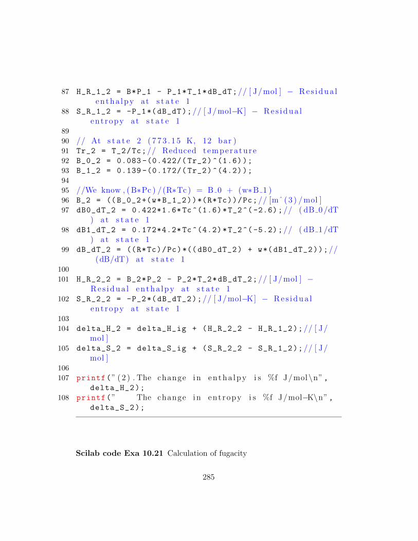
87 H_R_1_2 = B*P_1 - P_1*T_1*dB_dT;// [ J/mol ] − R e s i d u a len tha lpy at s t a t e 1

88 S_R_1_2 = -P_1*(dB_dT);// [ J/mol−K] − R e s i d u a len t ropy at s t a t e 1

89

90 // At s t a t e 2 ( 7 7 3 . 1 5 K, 12 bar )91 Tr_2 = T_2/Tc;// Reduced tempera tu r e92 B_0_2 = 0.083 -(0.422/( Tr_2)^(1.6));

93 B_1_2 = 0.139 -(0.172/( Tr_2)^(4.2));

94

95 //We know , ( B∗Pc ) /(R∗Tc ) = B 0 + (w∗B 1 )96 B_2 = ((B_0_2+(w*B_1_2))*(R*Tc))/Pc;// [mˆ ( 3 ) /mol ]97 dB0_dT_2 = 0.422*1.6* Tc ^(1.6)*T_2 ^( -2.6);// ( dB 0 /dT

) at s t a t e 198 dB1_dT_2 = 0.172*4.2* Tc ^(4.2)*T_2 ^( -5.2);// ( dB 1 /dT

) at s t a t e 199 dB_dT_2 = ((R*Tc)/Pc)*(( dB0_dT_2) + w*( dB1_dT_2));//

(dB/dT) at s t a t e 1100

101 H_R_2_2 = B_2*P_2 - P_2*T_2*dB_dT_2;// [ J/mol ] −R e s i d u a l en tha lpy at s t a t e 1

102 S_R_2_2 = -P_2*( dB_dT_2);// [ J/mol−K] − R e s i d u a len t ropy at s t a t e 1

103

104 delta_H_2 = delta_H_ig + (H_R_2_2 - H_R_1_2);// [ J/mol ]

105 delta_S_2 = delta_S_ig + (S_R_2_2 - S_R_1_2);// [ J/mol ]

106

107 printf(” ( 2 ) . The change i n en tha lpy i s %f J/mol\n”,delta_H_2);

108 printf(” The change i n ent ropy i s %f J/mol−K\n”,delta_S_2);

Scilab code Exa 10.21 Calculation of fugacity

285

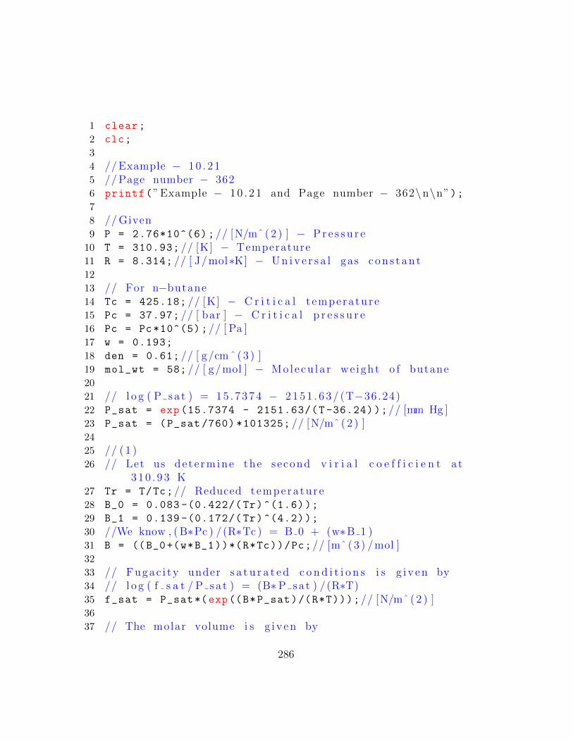
1 clear;

2 clc;

3


8 // Given9 P = 2.76*10^(6);// [N/mˆ ( 2 ) ] − P r e s s u r e10 T = 310.93; // [K] − Temperature11 R = 8.314; // [ J/mol∗K] − U n i v e r s a l gas c o n s t a n t12

13 // For n−butane14 Tc = 425.18; // [K] − C r i t i c a l t empera tu r e15 Pc = 37.97; // [ bar ] − C r i t i c a l p r e s s u r e16 Pc = Pc *10^(5);// [ Pa ]17 w = 0.193;

18 den = 0.61; // [ g/cm ˆ ( 3 ) ]19 mol_wt = 58; // [ g/mol ] − Molecu l a r we ight o f butane20

21 // l o g ( P sa t ) = 1 5 . 7 3 7 4 − 2 1 5 1 . 6 3 / (T−36 .24)22 P_sat = exp (15.7374 - 2151.63/(T -36.24));// [mm Hg ]23 P_sat = (P_sat /760) *101325; // [N/mˆ ( 2 ) ]24

25 // ( 1 )26 // Let us de t e rmine the second v i r i a l c o e f f i c i e n t at

3 1 0 . 9 3 K27 Tr = T/Tc;// Reduced tempera tu r e28 B_0 = 0.083 -(0.422/( Tr)^(1.6));

29 B_1 = 0.139 -(0.172/( Tr)^(4.2));

30 //We know , ( B∗Pc ) /(R∗Tc ) = B 0 + (w∗B 1 )31 B = ((B_0+(w*B_1))*(R*Tc))/Pc;// [mˆ ( 3 ) /mol ]32

33 // Fugac i ty under s a t u r a t e d c o n d i t i o n s i s g i v e n by34 // l o g ( f s a t / P sa t ) = (B∗P sa t ) /(R∗T)35 f_sat = P_sat *(exp((B*P_sat)/(R*T)));// [N/mˆ ( 2 ) ]36

37 // The molar volume i s g i v e n by

286

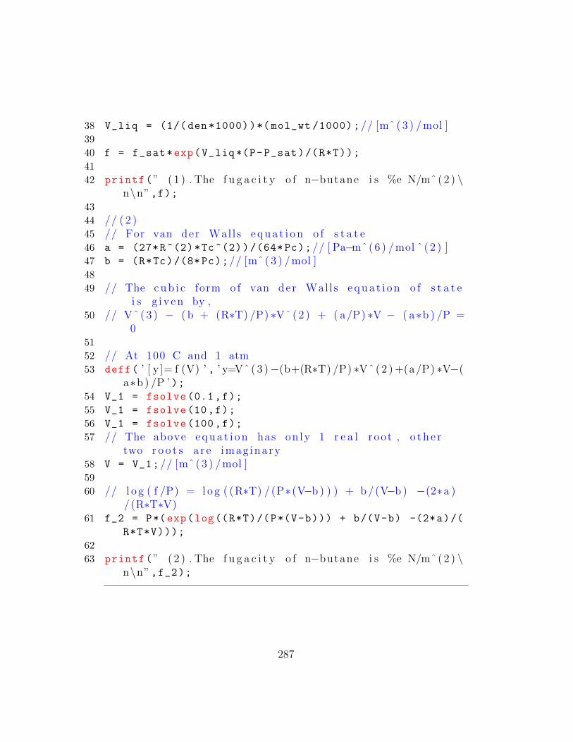
38 V_liq = (1/( den *1000))*( mol_wt /1000);// [mˆ ( 3 ) /mol ]39

40 f = f_sat*exp(V_liq *(P-P_sat)/(R*T));

41

42 printf(” ( 1 ) . The f u g a c i t y o f n−butane i s %e N/mˆ ( 2 ) \n\n”,f);

43



50 // Vˆ ( 3 ) − ( b + (R∗T) /P) ∗Vˆ ( 2 ) + ( a/P) ∗V − ( a∗b ) /P =0

51

52 // At 100 C and 1 atm53 deff( ’ [ y ]= f (V) ’ , ’ y=Vˆ ( 3 )−(b+(R∗T) /P) ∗Vˆ ( 2 ) +(a/P) ∗V−(

a∗b ) /P ’ );54 V_1 = fsolve (0.1,f);

55 V_1 = fsolve (10,f);

56 V_1 = fsolve (100,f);

57 // The above e q u a t i o n has on ly 1 r e a l root , o t h e rtwo r o o t s a r e imag ina ry

58 V = V_1;// [mˆ ( 3 ) /mol ]59

60 // l o g ( f /P) = l o g ( (R∗T) /(P∗ (V−b ) ) ) + b /(V−b ) −(2∗a )/(R∗T∗V)

61 f_2 = P*(exp(log((R*T)/(P*(V-b))) + b/(V-b) -(2*a)/(

R*T*V)));

62

63 printf(” ( 2 ) . The f u g a c i t y o f n−butane i s %e N/mˆ ( 2 ) \n\n”,f_2);

287

Scilab code Exa 10.22 Calculation of enthalpy change

1 clear;

2 clc;

3


8 // Given9 T = 50+273.15; // [K] − Temperature

10 P = 25*10^(3);// [ Pa ] − P r e s s u r e11 y1 = 0.5; // [ mol ] − mole f r a c t i o n o f equ imo l a r

mixture12 y2 = 0.5;


15 // For component 1 ( methyl e t h y l ke tone )16 Tc_1 = 535.5; // [K] − C r i t i c a l t empera tu r e17 Pc_1 = 41.5*10^(5);// [N/mˆ ( 2 ) ] − C r i t i c a l p r e s s u r e18 Vc_1 = 267; // [ cm ˆ ( 3 ) /mol ] − C r i t i c a l volume19 Zc_1 = 0.249; // C r i t i c a l c o m p r e s s i b i l i t y f a c t o r20 w_1 = 0.323; // a c e n t r i c f a c t o r21

22 // For component 2 ( t o l u e n e )23 Tc_2 = 591.8; // [K]24 Pc_2 = 41.06*10^(5);// [N/mˆ ( 2 ) ]25 Vc_2 = 316; // [ cm ˆ ( 3 ) /mol ]26 Zc_2 = 0.264;

27 w_2 = 0.262;

28

29 // For e q u a t i o n o f s t a t e Z = 1 + B/V30 // For component 1 , l e t us c a l c u l a t e B and dB/dT31 Tr_1 = T/Tc_1;// Reduced tempera tu r e32 //At reduced tempera tu r e33 B1_0 = 0.083 -(0.422/( Tr_1)^(1.6));

34 B1_1 = 0.139 -(0.172/( Tr_1)^(4.2));

35 //We know , ( B∗Pc ) /(R∗Tc ) = B 0+(w∗B 1 )

288

36 B_11 = ((B1_0+(w_1*B1_1))*(R*Tc_1))/Pc_1;// [mˆ ( 3 ) /mol−K]

37 dB0_dT_1 = 0.422*1.6* Tc_1 ^(1.6)*T^( -2.6);// [mˆ ( 3 ) /mol−K] − ( dB 0 /dT)


39 dB_dT_1 = ((R*Tc_1)/Pc_1)*(( dB0_dT_1) + w_1*(

dB1_dT_1));// [mˆ ( 3 ) /mol−K] − (dB/dT)40


45 B2_1 = 0.139 - (0.172/( Tr_2)^(4.2));

46 B_22 = ((B2_0+(w_2*B2_1))*(R*Tc_2))/Pc_2;// [mˆ ( 3 ) /mol ]



49 dB_dT_2 = ((R*Tc_2)/Pc_2)*(( dB0_dT_2) + w_2*(

dB1_dT_2));// [mˆ ( 3 ) /mol−K] − (dB/dT)50

51 // For c r o s s c o e f f c i e n t , l e t us c a l c u l a t e B and dB/dT52 Tc_12 = (Tc_1*Tc_2)^(1/2);// [K]53 w_12 = (w_1 + w_2)/2;

54 Zc_12 = (Zc_1 + Zc_2)/2;

55 Vc_12 = ((( Vc_1)^(1/3) + (Vc_2)^(1/3))/2) ^(3);// [ cmˆ ( 3 ) /mol ]


59 //Now we have , ( B 12∗Pc 12 ) /(R∗Tc 12 ) = B 0+(w 12∗B 1)



289

64 B_1 = 0.139 - (0.172/( Tr_12)^(4.2));

65 B_12 = ((B_0 + (w_12*B_1))*R*Tc_12)/Pc_12;// [mˆ ( 3 ) /mol ]

66 dB0_dT_12 = 0.422*1.6* Tc_12 ^(1.6)*T^( -2.6);// [mˆ ( 3 )/mol−K] − ( dB 0 /dT)

67 dB1_dT_12 = 0.172*4.2* Tc_12 ^(4.2)*T^( -5.2);// [mˆ ( 3 )/mol−K] − ( dB 1 /dT)

68 dB_dT_12 = ((R*Tc_12)/Pc_12)*(( dB0_dT_12) + w_12*(

dB1_dT_12));// [mˆ ( 3 ) /mol−K] − (dB/dT) 1269

70 // For the mixture71 B = y1^(2)*B_11 + 2*y1*y2*B_12 + y2^(2)*B_22;// [m

ˆ ( 3 ) /moL ]72

73 // The e q u a t i o n o f s t a t e can be w r i t t e n as74 // Vˆ ( 2 ) − ( (R∗T) /P) − (B∗R∗T) /P = 075 // Vˆ ( 2 ) − 0 . 1 0 7 5∗V + 1.737∗10ˆ( −4) = 076 deff( ’ [ y ]= f (V) ’ , ’ y=Vˆ ( 2 ) − 0 . 1 0 7 5∗V + 1.737∗10ˆ( −4) ’

);

77 V1 = fsolve (0.1,f);

78 V2 = fsolve(1,f);

79 // We w i l l c o n s i d e r the r o o t which i s near to R∗T/P80 V = V1;

81 // dB/dT = y 1 ˆ ( 2 ) ∗dB 11 /dT + y 2 ˆ ( 2 ) ∗dB 22 /dT + 2∗y 1 ∗ y 2 ∗dB 12 /dT

82 dB_dT = y1^(2)*dB_dT_1 + y2^(2)*dB_dT_2 + 2*y1*y2*

dB_dT_12;// [mˆ ( 3 ) /mol−K]83

84 // For e q u a t i o n o f s t a t e Z = 1 + B/V85 H_R = (B*R*T)/V - ((R*T^(2))/V)*dB_dT;// [ J/mol ]86

87 printf(” ( 1 ) . The v a l u e o f H R f o r the mixture u s i n gv i r i a l e q u a t i o n o f s t a t e i s %f J/mol\n\n”,H_R);

88

89 // ( 2 )90 // For van der Wal ls e q u a t i o n o f s t a t e91 a_11 = (27*R^(2)*Tc_1 ^(2))/(64* Pc_1);// [ Pa−mˆ ( 6 ) /mol

ˆ ( 2 ) ]

290

92 a_22 = (27*R^(2)*Tc_2 ^(2))/(64* Pc_2);// [ Pa−mˆ ( 6 ) /molˆ ( 2 ) ]

93 a_12 = (a_11*a_22)^(1/2);

94 b_1 = (R*Tc_1)/(8* Pc_1);// [mˆ ( 3 ) /mol ]95 b_2 = (R*Tc_2)/(8* Pc_2);// [mˆ ( 3 ) /mol ]96

97 // For the mixture98 a = y1^(2)*a_11 + y2^(2)*a_22 + 2*y1*y2*a_12;// [ Pa−m

ˆ ( 6 ) /mol ˆ ( 2 ) ]99 b = y1*b_1 + y2*b_2;// [mˆ ( 3 ) /mol ]

100

101 // From the c u b i c form o f van der Wal ls e q u a t i o n o fs t a t e

102 deff( ’ [ y ]= f 1 (V) ’ , ’ y=Vˆ ( 3 )−(b+(R∗T) /P) ∗Vˆ ( 2 ) +(a/P) ∗V−(a∗b ) /P ’ );

103 V2_1 = fsolve (0.1,f1);

104 V2_2 = fsolve (10,f1);

105 V2_3 = fsolve (100,f1);

106 // The l a r g e s t r o o t i s c o n s i d e r e d107 V_2 = V2_1;

108

109 // The r e s i d u a l en tha lpy i s g i v e n by110 H_R_2 = P*V_2 - R*T -a/V_2;// [ J/mol ]111

112 printf(” ( 2 ) . The v a l u e o f H R f o r the mixture u s i n gvan der Wal ls e q u a t i o n o f s t a t e i s %f J/mol\n\n”,H_R_2);

Scilab code Exa 10.23 Calculation of fugacity of water vapour

1 clear;

2 clc;

3

4 // Example − 1 0 . 2 35 // Page number − 366

291

6 printf(” Example − 1 0 . 2 3 and Page number − 366\n\n”);7

8 // Given9 T = 320 + 273.15; // [K]10 R = 8.314; // [ J/mol∗K] − U n i v e r s a l gas c o n s t a n t11

12 // For water13 Tc = 647.1; // [K]14 Pc = 220.55; // [ bar ]15 Pc = Pc *10^(5);// [ Pa ]16


18 // Vˆ ( 3 ) − ( (R∗T) /P) ∗Vˆ ( 2 ) − ( ( b 1 ˆ ( 2 ) ) + ( ( b 1 ∗R∗T)/P) − ( a /(Tˆ ( 1 / 2 ) ∗P) ) ∗V − ( a∗b ) /(Tˆ ( 1 / 2 ) ∗P) = 0

19

20 // At 320 C and 70 bar p r e s s u r e21 P_1 = 70; // [ bar ]22 P_1 = P_1 *10^(5);// [ Pa ]23

24 a = (0.42748*(R^(2))*(Tc ^(2.5)))/Pc;// [ Pa∗mˆ ( 6 ) ∗Kˆ ( 1 / 2 ) /mol ]

25 b = (0.08664*R*Tc)/Pc;// [mˆ ( 3 ) /mol ]26 // S o l v i n g the c u b i c e q u a t i o n27 deff( ’ [ y ]= f 1 (V) ’ , ’ y=Vˆ ( 3 ) −((R∗T) / P 1 ) ∗Vˆ ( 2 ) −((b ˆ ( 2 ) )

+((b∗R∗T) / P 1 )−(a /(Tˆ ( 1 / 2 ) ∗P 1 ) ) ) ∗V−(a∗b ) /(Tˆ ( 1 / 2 ) ∗P 1 ) ’ );

28 V1=fsolve(1,f1);

29 V2=fsolve (10,f1);

30 V3=fsolve (100,f1);

31 // The l a r g e s t r o o t i s c o n s i d e r e d because at 320 Cand 70 bar vapour phase e x i s t s .

32 V_1 = V1;// [mˆ ( 3 ) /mol ]33 // Thus c o m p r e s s i b i l i t y f a c t o r i s34 Z_1 = (P_1*V_1)/(R*T);

35

36 // For Red l i ch−Kwong e q u a t i o n o f s t a t e37 // l o g ( f /P) = Z − 1 − l o g ( V 1 /( V 1−b ) ) + ( a /( b∗R∗ (T

292

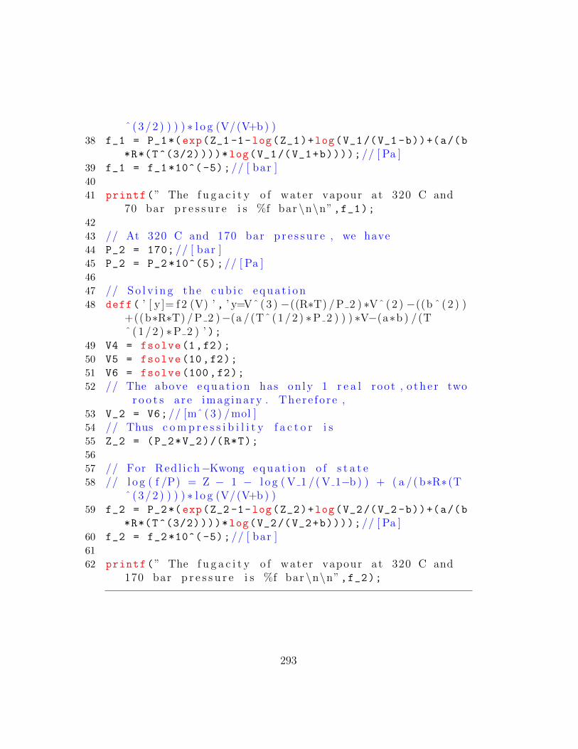
ˆ ( 3 / 2 ) ) ) ) ∗ l o g (V/(V+b ) )38 f_1 = P_1*(exp(Z_1 -1-log(Z_1)+log(V_1/(V_1 -b))+(a/(b

*R*(T^(3/2))))*log(V_1/(V_1+b))));// [ Pa ]39 f_1 = f_1 *10^( -5);// [ bar ]40

41 printf(” The f u g a c i t y o f water vapour at 320 C and70 bar p r e s s u r e i s %f bar \n\n”,f_1);

42

43 // At 320 C and 170 bar p r e s s u r e , we have44 P_2 = 170; // [ bar ]45 P_2 = P_2 *10^(5);// [ Pa ]46

47 // S o l v i n g the c u b i c e q u a t i o n48 deff( ’ [ y ]= f 2 (V) ’ , ’ y=Vˆ ( 3 ) −((R∗T) / P 2 ) ∗Vˆ ( 2 ) −((b ˆ ( 2 ) )

+((b∗R∗T) / P 2 )−(a /(Tˆ ( 1 / 2 ) ∗P 2 ) ) ) ∗V−(a∗b ) /(Tˆ ( 1 / 2 ) ∗P 2 ) ’ );

49 V4 = fsolve(1,f2);

50 V5 = fsolve (10,f2);

51 V6 = fsolve (100,f2);

52 // The above e q u a t i o n has on ly 1 r e a l root , o t h e r twor o o t s a r e imag ina ry . The r e f o r e ,

53 V_2 = V6;// [mˆ ( 3 ) /mol ]54 // Thus c o m p r e s s i b i l i t y f a c t o r i s55 Z_2 = (P_2*V_2)/(R*T);

56

57 // For Red l i ch−Kwong e q u a t i o n o f s t a t e58 // l o g ( f /P) = Z − 1 − l o g ( V 1 /( V 1−b ) ) + ( a /( b∗R∗ (T

ˆ ( 3 / 2 ) ) ) ) ∗ l o g (V/(V+b ) )59 f_2 = P_2*(exp(Z_2 -1-log(Z_2)+log(V_2/(V_2 -b))+(a/(b

*R*(T^(3/2))))*log(V_2/(V_2+b))));// [ Pa ]60 f_2 = f_2 *10^( -5);// [ bar ]61

62 printf(” The f u g a c i t y o f water vapour at 320 C and170 bar p r e s s u r e i s %f bar \n\n”,f_2);

293

Scilab code Exa 10.24 Determination of change in internal energy

1 clear;

2 clc;

3


8 // Given9 Vol = 0.057; // [mˆ ( 3 ) ] − Volume o f c a r t y r e10 P_1 = 300; // [ kPa ] − I n i t i a l p r e s s u r e11 P_1 = P_1 *10^(3);// [ Pa ]12 T_1 = 300; // [K] − I n i t i a l t empera tu re13 P_2 = 330; // [ kPa ] − Finna l p r e s s u r e14 P_2 = P_2 *10^(3);// [ Pa ]15 R = 8.314; // [ J/mol∗K] − U n i v e r s a l gas c o n s t a n t16 Cv_0 = 21; // [ J/mol−K] − Heat c a p a c i t y f o r a i r17

18 // For oxygen19 Tc_O2 = 154.6; // [K] − C r i t i c a l t empera tu r e20 Pc_O2 = 50.43; // [ bar ] − C r i t i c a l p r e s s u r e21 Pc_O2 = Pc_O2 *10^(5);// [ Pa ]22 y1 = 0.21; // − Mole f r a c t i o n o f oxygen23 // For n i t r o g e n24 Tc_N2 = 126.2; // [K] − C r i t i c a l t empera tu r e25 Pc_N2 = 34.00; // [ bar ] − C r i t i c a l p r e s s u r e26 Pc_N2 = Pc_N2 *10^(5);// [ Pa ]27 y2 = 0.79; // − Mole f r a c t i o n o f n i t r o g e n28

29 // ( 1 )30 // Assuming i d e a l gas behav i ou r . The volume rema ins

the same , t h e r e f o r e , we g e t31 // P 1 / T 1 = P 2 / T 232 T_2 = P_2*(T_1/P_1);// [K]33

34 n = (P_1*Vol)/(R*T_1);// [ mol ] − Number o f moles35 delta_U = n*Cv_0*(T_2 -T_1);// [ J ]

294

36

37 printf(” ( 1 ) . The change i n i n t e r n a l ene rgy ( f o ri d e a l gas behav i ou r ) i s %f J\n\n”,delta_U);

38

39 // ( 2 )40 // For van der Wal ls e q u a t i o n o f s t a t e41 a_O2 = (27*R^(2)*Tc_O2 ^(2))/(64* Pc_O2);// [ Pa−mˆ ( 6 ) /

mol ˆ ( 2 ) ]42 a_N2 = (27*R^(2)*Tc_N2 ^(2))/(64* Pc_N2);// [ Pa−mˆ ( 6 ) /

mol ˆ ( 2 ) ]43 a_12 = (a_O2*a_N2)^(1/2);

44 b_O2 = (R*Tc_O2)/(8* Pc_O2);// [mˆ ( 3 ) /mol ]45 b_N2 = (R*Tc_N2)/(8* Pc_N2);// [mˆ ( 3 ) /mol ]46

47 // For the mixture48 a = y1^(2)*a_O2 + y2^(2)*a_N2 + 2*y1*y2*a_12;// [ Pa−m

ˆ ( 6 ) /mol ˆ ( 2 ) ]49 b = y1*b_O2 + y2*b_N2;// [mˆ ( 3 ) /mol ]50

51 // From the c u b i c form o f van der Wal ls e q u a t i o n o fs t a t e

52 // At 300 K and 300 kPa ,53 deff( ’ [ y ]= f 1 (V) ’ , ’ y=Vˆ ( 3 )−(b+(R∗T 1 ) / P 1 ) ∗Vˆ ( 2 ) +(a/

P 1 ) ∗V−(a∗b ) / P 1 ’ );54 V_1 = fsolve (0.1,f1);

55 V_2 = fsolve (10,f1);

56 V_3 = fsolve (100,f1);

57 // The above e q u a t i o n has on ly 1 r e a l root , o t h e rtwo r o o t s a r e imag ina ry

58 V = V_1;// [mˆ ( 3 ) /mol ]59

60 // Now at P = 330 kPa and at molar volume V61 // The van der Wal ls e q u a t i o n o f s t a t e i s62 // (P + a/Vˆ ( 2 ) ) ∗ (V − b ) = R∗T63 T_2_prime = ((P_2 + a/V^(2))*(V - b))/R;// [K]64 n_prime = Vol/V;// [ mol ]65

66 // Tota l change i n i n t e r n a l ene rgy i s g i v e n by

295

67 // d e l t a U p r i m e = n pr ime ∗ d e l t a U i g + n pr ime ∗ (U R 2 − U R 1 )

68 // d e l t a U p r i m e = n pr ime ∗Cv 0 ∗ ( T 2 pr ime − T 1 ) +n pr ime ∗a (1/ V 2 − 1/ V 1 ) ;

69 // S i n c e V 1 = V 2 = V, t h e r e f o r e70 delta_U_prime = n_prime*Cv_0*( T_2_prime - T_1);

71

72 printf(” ( 2 ) . The change i n i n t e r n a l ene rgy ( f o r vander Wal ls e q u a t i o n o f s t a t e ) i s %f J\n\n”,delta_U_prime);

Scilab code Exa 10.25 Calculation of enthalpy and entropy change

1 clear;

2 clc;

3 funcprot (0);

4


9 // Given10 T_1 = 150 + 273.15; // [K] − I n i t i a l emperature11 T_2 = T_1;// I s o t h e r m a l p r o c e s s12 P_1 = 100*10^(3);// [ Pa ] − I n i t i a l p r e s s u r e13 P_2 = 450*10^(3);// [ Pa ] − F i n a l p r e s s u r e14 R = 8.314; // [ J/mol∗K] − U n i v e r s a l gas c o n s t a n t15 // For water16 Tc = 647.1; // [K] − C r i t i c a l t empera tu r e17 Pc = 220.55; // [ bar ] − C r i t i c a l p r e s s u r e18 Pc = Pc *10^(5);

19 w = 0.345;

20 Mol_wt = 18.015; // [ g/mol ] − Molecu l a r we ight o fwater

21 Cp_0 = 4.18; // [ J/mol−K] − Standard heat c a p a c i t y o f

296

water22

23 // Both phase s a r e s u p e r h e a t e d vapour phase s becauseat 150 C the vapour p r e s s u r e o f steam i s 4 . 6 7

bar and both o p e r a t i n g p r e s s u r e s a r e belows a t u r a t e d p r e s s u r e .

24 // In Peng−Robinson e q u a t i o n o f s t a t e25 m = 0.37464 + 1.54226*w - 0.26992*w^(2);

26 // At T 1 and P 1 , we have27 Tr = T_1/Tc;

28 alpha = (1 + m*(1 - Tr ^(1/2)))^(2);


30 b = (0.07780*R*Tc)/Pc;// [mˆ ( 3 ) /mol ]31

32 // Cubuc form o f Peng−Robinson e q u a t i o n o f s t s t e i sg i v e n by

33 // Vˆ ( 3 ) +(b−(R∗T) /P) ∗Vˆ ( 2 ) −((3∗b ˆ ( 2 ) ) +((2∗R∗T∗b ) /P)−(a/P) ) ∗V+b ˆ ( 3 ) +((R∗T∗ ( b ˆ ( 2 ) ) /P) −((a∗b ) /P) =0;

34 // S o l v i n g the c u b i c e q u a t i o n35 deff( ’ [ y ]= f (V) ’ , ’ y=Vˆ ( 3 ) +(b−(R∗T 1 ) / P 1 ) ∗Vˆ ( 2 ) −((3∗b

ˆ ( 2 ) ) +((2∗R∗T 1∗b ) / P 1 )−(a/ P 1 ) ) ∗V+b ˆ ( 3 ) +((R∗T 1∗ ( b ˆ ( 2 ) ) ) / P 1 ) −((a∗b ) / P 1 ) ’ );

36 V1 = fsolve(-1,f);




s y s t e m i s gas41 V_1 = V3;// [mˆ ( 3 ) /mol ]42 // Thus c o m p r e s s i b i l i t y f a c t o r i s43 Z_1 = (P_1*V_1)/(R*T_1);

44

45 // At T 2 and P 2 , we have46 // Cubuc form o f Peng−Robinson e q u a t i o n o f s t s t e i s

g i v e n by47 // Vˆ ( 3 ) +(b−(R∗T) /P) ∗Vˆ ( 2 ) −((3∗b ˆ ( 2 ) ) +((2∗R∗T∗b ) /P)

−(a/P) ) ∗V+b ˆ ( 3 ) +((R∗T∗ ( b ˆ ( 2 ) ) /P) −((a∗b ) /P) =0;

297

48 // S o l v i n g the c u b i c e q u a t i o n49 deff( ’ [ y ]= f (V) ’ , ’ y=Vˆ ( 3 ) +(b−(R∗T 2 ) / P 2 ) ∗Vˆ ( 2 ) −((3∗b

ˆ ( 2 ) ) +((2∗R∗T 2∗b ) / P 2 )−(a/ P 2 ) ) ∗V+b ˆ ( 3 ) +((R∗T 2∗ ( b ˆ ( 2 ) ) ) / P 2 ) −((a∗b ) / P 2 ) ’ );

50 V4 = fsolve(-1,f);




s y s t e m i s gas55 V_2 = V6;// [mˆ ( 3 ) /mol ]56 // Thus c o m p r e s s i b i l i t y f a c t o r i s57 Z_2 = (P_2*V_2)/(R*T_2);

58

59 // In the Peng−Robinson e q u a t i o n o f s t s t e60 // da/dT = −(a∗m) / ( ( a lpha ∗T∗Tc ) ˆ ( 1 / 2 ) )61 // The r e s i d u a l en tha lpy i s g i v e n by62 // H R = R∗T∗ (Z−1) + ( ( (T∗ ( da dT ) )−a ) / ( 2∗2 ˆ ( 1 / 2 ) ∗b ) )

∗ l o g ( ( Z+(1+2ˆ(1/2) ∗ ( (P∗b ) /(R∗T) ) ) ) /(Z+(1−2ˆ(1/2)∗ ( (P∗b ) /(R∗T) ) ) ) )

63

64 // At s t a t e 165 da_dT_1 = -(a*m)/(( alpha*T_1*Tc)^(1/2));// [ Pa∗mˆ ( 6 ) /

mol ˆ ( 2 ) ]66 H_R_1 = R*T_1*(Z_1 -1) + (((T_1*( da_dT_1))-a)

/(2*(2^(1/2))*b))*log((Z_1 +(1+2^(1/2))*((P_1*b)/(

R*T_1)))/(Z_1 +(1 -2^(1/2))*((P_1*b)/(R*T_1))));

67

68 // At s t a t e 269 da_dT_2 = -(a*m)/(( alpha*T_2*Tc)^(1/2));// [ Pa∗mˆ ( 6 ) /

mol ˆ ( 2 ) ]70 H_R_2 = R*T_2*(Z_2 -1) + (((T_2*( da_dT_2))-a)

/(2*2^(1/2)*b))*log((Z_2 +(1+2^(1/2))*((P_2*b)/(R*

T_1)))/(Z_2 +(1 -2^(1/2))*((P_2*b)/(R*T_1))));

71

72

73 // S i n c e the t empera tu r e i s the same , t h e r e f o r e i d e a lgas change i n en tha lpy i s z e r o and thus

298

74 delta_H = H_R_2 - H_R_1 ;; // [ J/mol ]75 delta_H = delta_H/Mol_wt;// [ kJ/ kg ]76

77 // The r e s i d u a l en t ropy r e l a t i o n f o r a s u b s t a n c ef o l l o w i n g Peng − Robinson e q u a t i o n o f s t a t e i a

78 // S R = R∗ l o g (Z − (P∗b ) /(R∗T) ) + ( da dT / ( 2∗2 ˆ ( 1 / 2 ) ∗b ) ) ∗ l o g ( ( Z+(1+2ˆ(1/2) ) ∗ ( (P∗b ) /(R∗T) ) ) /(Z+(1−2ˆ(1/2) ) ∗ ( (P∗b ) /(R∗T) ) ) )

79

80 // The r e s i d u a l en t ropy at s t a t e 1 i s81 S_R_1 = R*log(Z_1 - (P_1*b)/(R*T_1)) + (da_dT_1

/(2*2^(1/2)*b))*log((Z_1 +(1+2^(1/2))*((P_1*b)/(R*

T_1)))/(Z_1 +(1 -2^(1/2))*(( P_1*b)/(R*T_1))));

82

83 // The r e s i d u a l en t ropy at s t a t e 2 i s84 S_R_2 = R*log(Z_2 - (P_2*b)/(R*T_2)) + (da_dT_2

/(2*2^(1/2)*b))*log((Z_2 +(1+2^(1/2))*((P_2*b)/(R*

T_2)))/(Z_2 +(1 -2^(1/2))*(( P_2*b)/(R*T_2))));

85

86 delta_S_R = S_R_2 - S_R_1;// [ J/mol−K]87

88 // The i d e a l gas change i n ent ropy i s89 delta_S_ig = Cp_0*log(T_2/T_1) - R*log(P_2/P_1);// [ J

/mol−K]90

91 // T h e r e f o r e92 delta_S = delta_S_R + delta_S_ig;// [ J/mol−K]93

94 printf(” The en tha lpy change i s g i v e n by , d e l t a H =%f kJ/mol\n\n”,delta_H);

95 printf(” The ent ropy change i s g i v e n by , d e l t a S =%f J/mol−K\n\n”,delta_S);

Scilab code Exa 10.26 Calculation of final temperature and pressure

299

1 clear;

2 clc;

3 funcprot (0);

4


9 // Given10 Vol = 0.15; // [mˆ ( 3 ) ]11 T_1 = 170; // [K] − I n i t i a l emperature12 P_1 = 100; // [ bar ] − I n i t i a l p r e s s u r e13 P_1 = P_1 *10^(5);// [ Pa ]14 R = 8.314; // [ J/mol∗K] − U n i v e r s a l gas c o n s t a n t15 // For n i t r o g e n16 Tc = 126.2; // [K] − C r i t i c a l t empeature17 Pc = 34; // [ bar ] − C r i t i c a l p r e s s u r e18 Pc = Pc *10^(5);// [ Pa ]19 w = 0.038;

20 // Cp 0 = 27.2+4.2∗10ˆ( −3) ∗T21



28 // Vˆ ( 3 ) − ( b + (R∗T) /P) ∗Vˆ ( 2 ) + ( a/P) ∗V − ( a∗b ) /P =0

29 // On s i m p l i f i c a t i o n the e q u a t i o n changes to30 // Vˆ ( 3 ) − 1 . 7 9 9 ∗ 1 0 ˆ ( 4 ) ∗Vˆ ( 2 ) + 1.366∗10ˆ( −8) ∗V −

5 .269∗10ˆ( −13) = 031

32 // S o l v i n g the c u b i c e q u a t i o n33 deff( ’ [ y ]= f (V) ’ , ’ y=Vˆ ( 3 ) −1.799∗10ˆ(−4) ∗Vˆ ( 2 ) +

1.366∗10ˆ( −8) ∗V − 5 .269∗10ˆ( −13) ’ );34 V1 = fsolve(1,f);

300

35 V2 = fsolve (10,f);

36 V3 = fsolve (100,f);

37 // The above e q u a t i o n has on ly 1 r e a l root , o t h e rtwo r o o t s a r e imagimnary

38 V_1 = V1;// [mˆ ( 3 ) /mol ]39 // Thus t o t a l number o f moles i s g i v e n by40 n_1 = Vol/V_1;// [ mol ]41

42 // A f t e r 500 mol a r e withdrawn , the f i n a l number o fmoles i s g i v e n by

43 n_2 = n_1 - 500; // [ mol ]44 // Thus molar volume at f i n a l s t a t e i s45 V_2 = Vol/n_2;// [mˆ ( 3 ) /mol ]46

47 // The i d e a l en t ropy change i s guven by48 // d e l t a S i g = i n t e g r a t e ( ’ 27 . 2+4 .2∗10ˆ( −3) ∗T’ , ’ T’ ,

T 1 , T 2 ) − R∗ l o g ( P 2 / P 1 ) ;49 // The r e s i d u a l en t ropy change i s g i v e n by50 // d e l t a S R = R∗ l o g ( ( P 2 ∗ ( V 2−b ) ) /(R∗T 2 ) ) − R∗ l o g

( ( P 1 ∗ ( V 1−b ) ) /(R∗T 1 ) )51 // d e l t a S = d e l t a S i g = d e l t a S R52 // d e l t a S = i n t e g r a t e ( ’ 27 . 2+4 .2∗10ˆ( −3) ∗T’ , ’ T’ , T 1 ,

T 2 ) + R∗ l o g ( ( V 2−b ) /( V 1−b ) ) ;53 // During d i s c h a r g i n g d e l t a S = 0 , thus on

s i m p l i f i c a t i o n we g e t54 // 1 8 . 8 8 6∗ l o g ( T 2 ) + 4.2∗10ˆ( −3) ∗T 2 − 9 2 . 9 3 7 = 055 // S o l v i n g the above e q u a t i o n we g e t56 deff( ’ [ y ]= f 1 ( T 2 ) ’ , ’ y =18.886∗ l o g ( T 2 ) + 4.2∗10ˆ( −3) ∗

T 2 − 9 2 . 9 3 7 ’ );57 T_2 = fsolve(1,f1);

58

59 // Thus at T 2 ,60 P_2 = (R*T_2)/(V_2 -b) - a/V_2 ^(2);// [N/mˆ ( 2 ) ]61 P_2 = P_2 *10^( -5);// [ bar ]62

63 printf(” ( 1 ) . The f i n a l t empera tu re i s %f K\n”,T_2);64 printf(” The f i n a l p r e s s u r e i s %f bar \n\n”,P_2);65

301

66 // ( 2 )67 // In Peng−Robinson e q u a t i o n o f s t a t e68 m = 0.37464 + 1.54226*w - 0.26992*w^(2);

69 // At T 1 and P 1 , we have70 Tr = T_1/Tc;

71 alpha = (1 + m*(1 - Tr ^(1/2)))^(2);

72 a_2 = ((0.45724*(R*Tc)^(2))/Pc)*alpha;// [ Pa∗mˆ ( 6 ) /mol ˆ ( 2 ) ]

73 b_2 = (0.07780*R*Tc)/Pc;// [mˆ ( 3 ) /mol ]74

75 // Cubuc form o f Peng−Robinson e q u a t i o n o f s t s t e i sg i v e n by


77 // S o l v i n g the c u b i c e q u a t i o n78 deff( ’ [ y ]= f 2 (V) ’ , ’ y=Vˆ ( 3 ) +(b 2−(R∗T 1 ) / P 1 ) ∗Vˆ ( 2 )

−((3∗ b 2 ˆ ( 2 ) ) +((2∗R∗T 1∗ b 2 ) / P 1 )−( a 2 / P 1 ) ) ∗V+b 2 ˆ ( 3 ) +((R∗T 1 ∗ ( b 2 ˆ ( 2 ) ) ) / P 1 ) −(( a 2 ∗ b 2 ) / P 1 ) ’ );

79 V4 = fsolve(-1,f2);

80 V5 = fsolve(0,f2);

81 V6 = fsolve (0.006 ,f2);

82 //The above e q u a t i o n has on ly 1 r e a l root , the o t h e rtwo r o o t s a r e imag ina ry

83 V_1_2 = V6;// [mˆ ( 3 ) /mol ]84

85 // The number o f moles i n the i n i t i a l s t a t e i s g i v e nby

86 n_1_2 = Vol/V_1_2;// [ mol ]87 // A f t e r 500 mol a r e withdrawn , the f i n a l number o f

moles i s g i v e n by88 n_2_2 = n_1_2 - 500; // [ mol ]89 // Thus molar volume at f i n a l s t a t e i s90 V_2_2 = Vol/n_2_2;// [mˆ ( 3 ) /mol ]91

92 // At the f i n a l s t a t e the r e l a t i o n between p r e s s u r eand tempera tu r e i s

93 // P 2 2 = (R∗T 2 2 ) /( V 2 2−b 2 ) − a 2 / V 2 2 ˆ ( 2 )

302

94 // P 2 2 = 7 . 2 3 ∗ 1 0 ˆ ( 4 ) ∗T 2 − 3 . 9 3 ∗ 1 0 ˆ ( 7 ) ∗ a 295

96 // Now l e t us c a l c u l a t e the r e s i d u a l en t ropy ati n i t i a l s t a t e

97 Z_1 = (P_1*V_1_2)/(R*T_1);

98 da_dT_1 = -(a*m)/(( alpha*T_1*Tc)^(1/2));// [ Pa∗mˆ ( 6 ) /mol ˆ ( 2 ) ] − da/dT

99

100 // The r e s i d u a l en t ropy change f o r Peng−Robinsone q u a t i o b o f s t a t e i s g i v e n by

101 // S R = R∗ l o g (Z−(P∗b ) /(R∗T) ) + ( da dT / ( 2∗2 ˆ ( 1 / 2 ) ∗b )) ∗ l o g ( (V+(1+2ˆ(1/2) ) ∗b ) ) / ( (V+(1−2ˆ(1/2)∗b ) ) ) ) ;

102 S_R_1 = R*(log(Z_1 -(P_1*b_2)/(R*T_1))) + (da_dT_1

/(2*2^(1/2)*b_2))*(log((V_1_2 +(1+2^(1/2))*b_2)/(

V_1_2 +(1 -2^(1/2))*b_2)));

103

104 // The t o t a l en t ropy change i s g i v e n by105 // d e l t a S = d e l t a S i g + d e l t a S R106 // where , d e l t a S i g = i n t e g r a t e ( ’ 27 . 2+4 .2∗10ˆ( −3) ∗T

’ , ’ T’ , T 1 , T 2 2 ) − R∗ l o g ( P 2 2 / P 1 ) ;107 // and , P 2 2 = (R∗T 2 2 ) /( V 2 2−b 2 ) − a 2 / V 2 2

ˆ ( 2 )108 // On s i m p l i f i c a t i o n we ge t109 // d e l t a S = 2 7 . 2∗ l o g ( T 2 2−T 1 ) + 4.2∗10ˆ( −3) ∗ (

T 2 2−T 1 ) − R∗ l o g ( P 2 2 / P 1 ) + R∗ l o g ( Z 2−( P 2 2 ∗b ) /(R∗T 2 2 ) ) + 6226∗ ( da dT 2 ) + 9 . 2 2

110

111 // Now we have the de t e rmine the v a l u e o f T 2 2 suchtha t d e l t a S = 0

112 // S t a r t i n g with a t empera tu r e o f 150 K113 T_prime = 100; // [K]114 error = 10;


116 Tr_prime = T_prime/Tc;

117 alpha_prime = (1 + m*(1 - Tr_prime ^(1/2)))^(2);

118 a_prime = ((0.45724*(R*Tc)^(2))/Pc)*alpha_prime;

119 P_prime = 7.23*10^(4)*T_prime - 3.93*10^(7)*

a_prime;

303

120 Z_prime = (P_prime*V_2_2)/(R*T_prime);

121 da_dT_prime = -(a_prime*m)/(( alpha_prime*T_prime

*Tc)^(1/2));

122 delta_S = 27.2* log(T_prime/T_1) + 4.2*10^( -3) *(

T_prime -T_1) - R*log(P_prime/P_1) + R*log(

Z_prime -(( P_prime*b_2)/(R*T_prime))) + 6226*(

da_dT_prime) + 9.22;

123 error=abs(delta_S);


125 end

126

127 T_2_2 = T_prime;// [K] − F i n a l t empera tu r e128 P_2_2 = P_prime *10^( -5);// [ bar ] − F i n a l p r e s s u r e129

130 printf(” ( 2 ) . The f i n a l t empera tu re i s %f K\n”,T_2_2);

131 printf(” The f i n a l p r e s s u r e i s %f bar \n”,P_2_2);

Scilab code Exa 10.27 Calculation of vapour pressure

1 clear;

2 clc;

3 funcprot (0);

4


9 // Given10 T = 373.15; // [K]11 Tc = 562.16; // [K]12 Pc = 48.98; // [ bar ]13 Pc = Pc *10^(5);// [ Pa ]14 R = 8.314; // [ J/mol−K] − U n i v e r s a l gas c o n s t a n t15

304


17 // Vˆ ( 3 ) − ( (R∗T) /P) ∗Vˆ ( 2 ) − ( ( b 1 ˆ ( 2 ) ) + ( ( b 1 ∗R∗T)/P) − ( a /(Tˆ ( 1 / 2 ) ∗P) ) ∗V − ( a∗b ) /(Tˆ ( 1 / 2 ) ∗P) = 0

18

19 a = (0.42748*(R^(2))*(Tc ^(2.5)))/Pc;// [ Pa∗mˆ ( 6 ) ∗Kˆ ( 1 / 2 ) /mol ]

20 b = (0.08664*R*Tc)/Pc;// [mˆ ( 3 ) /mol ]21

22 // At 3 7 3 . 1 5 K, l e t us assume the p r e s s u r e to be 2 . 5bar and under t h e s e c o n d i t i o n s

23 P_1 = 2.5; // [ bar ]24 P_1 = P_1 *10^(5);// [ bar ]25

26 // Put t ing the v a l u e s i n R e d l i c h Kwong e q u a t i o n o fs t a t e , the e q u a t i o n becomes

27 // Vˆ ( 3 ) − 0 . 0 1 2 4∗Vˆ ( 2 ) + 8.326∗10ˆ( −6) ∗V −7 .74∗10ˆ( −10) = 0

28 // S o l v i n g the c u b i c e q u a t i o n29

30 deff( ’ [ y ]= f (V) ’ , ’ y=Vˆ ( 3 ) − 0 . 0 1 2 4∗Vˆ ( 2 ) +8.326∗10ˆ( −6) ∗V − 7 .74∗10ˆ( −10) ’ );

31 V1=fsolve(-9,f);

32 V2=fsolve (10,f);

33 V3=fsolve (0.1,f);

34 // The l a r g e s t r o o t and the s m a l l e s t r o o t i sc o n s i d e r e d f o r l i q u i d phase and vapour phaser e s p e c t i v e l y .

35 V_liq = V1;// [mˆ ( 3 ) /mol ] − Molar volume i n l i q u i dphase

36 V_vap = V3;// [mˆ ( 3 ) /mol ] − Molar volume i n vapourphase

37

38 // Let us c a l c u l a t e the f u g a c i t y o f vapour phase39 // l o g ( f v a p /P) = b /(V−b ) + l o g ( (R∗T) /(P∗ (V−b ) ) ) − (

a /(R∗Tˆ ( 1 . 5 ) ) ) ∗ ( 1 / (V+b ) − (1/ b ) ∗ l o g (V/(V+b ) ) )40 f_vap = P_1*exp(b/(V_vap -b) + log((R*T)/(P_1*(V_vap -

b))) - (a/(R*T^(1.5)))*(1/( V_vap+b) - (1/b)*log(

305

V_vap/(V_vap+b))));// [ Pa ]41

42 // Let us c a l c u l a t e the f u g a c i t y o f the l i q u i d phase43 f_liq = P_1*exp(b/(V_liq -b) + log((R*T)/(P_1*(V_liq -

b))) - (a/(R*T^(1.5)))*(1/( V_liq+b) - (1/b)*log(

V_liq/(V_liq+b))));

44

45

46 // The two f u g a c i t i e s a r e not same ; t h e r e f o r eano the r p r e s s u r e i s to be assumed . The newp r e s s u r e i s

47 P_new = P_1*(f_liq/f_vap);// [ Pa ]48

49 // At P new50 deff( ’ [ y ]= f 1 (V) ’ , ’ y=Vˆ ( 3 ) − ( (R∗T) /P new ) ∗Vˆ ( 2 ) − ( b

ˆ ( 2 ) + ( ( b∗R∗T) /P new ) − a /(Tˆ ( 1 / 2 ) ∗P new ) ) ∗V − (a∗b ) /(Tˆ ( 1 / 2 ) ∗P new ) ’ );

51 V4=fsolve(-9,f1);

52 V5=fsolve (10,f1);

53 V6=fsolve (0.1,f1);


55 V_liq_2 = V4;// [mˆ ( 3 ) /mol ] − Molar volume i n l i q u i dphase

56 V_vap_2 = V6;// [mˆ ( 3 ) /mol ] − Molar volume i n vapourphase

57

58 f_vap_prime = P_new*exp(b/(V_vap_2 -b) + log((R*T)/(

P_new*(V_vap_2 -b))) - (a/(R*T^(1.5)))*(1/( V_vap_2

+b) - (1/b)*log(V_vap_2 /( V_vap_2+b))));// [ Pa ]59 f_liq_prime = P_new*exp(b/(V_liq_2 -b) + log((R*T)/(

P_new*(V_liq_2 -b))) - (a/(R*T^(1.5)))*(1/( V_liq_2

+b) - (1/b)*log(V_liq_2 /( V_liq_2+b))));

60

61 // S i n c e the f u g a c i t i e s o f l i q u i d and vapourp h a s e s a r e a lmost same the assumed p r e s s u r e may be

taken as vapour p r e s s u r e at 3 7 3 . 1 5 K

306

62 P_new = P_new *10^( -5);// [ bar ]63

64 printf(” The vapour p r e s s u r e o f benzene u s i n gR e d l i c h Kwong e q u a t i o n o f s t a t e i s %f bar \n”,P_new);

Scilab code Exa 10.28 Determination of vapour pressure

1 clear;

2 clc;

3 funcprot (0);

4


9 // Given10 T = 150 + 273.15; // [K]11 Tc = 647.1; // [K]12 Pc = 220.55; // [ bar ]13 Pc = Pc *10^(5);// [ Pa ]14 w = 0.345;

15 R = 8.314; // [ J/mol−K] − U n i v e r s a l gas c o n s t a n t16

17 // Let us assume a p r e s s u r e o f 100 kPa .18 P_1 = 100*10^(3);// [ Pa ]19

20 // At 100 kPa and 4 2 3 . 1 5 K, from Peng−Robinsone q u a t i o n o f s t s t e

21 m = 0.37464 + 1.54226*w - 0.26992*w^(2);

22 Tr = T/Tc;

23 alpha = (1 + m*(1 - Tr ^(1/2)))^(2);


25 b = (0.07780*R*Tc)/Pc;// [mˆ ( 3 ) /mol ]

307

26 // Cubic form o f Peng−Robinson e q u a t i o n o f s t s t e i sg i v e n by


28 // S o l v i n g the c u b i c e q u a t i o n29 deff( ’ [ y ]= f (V) ’ , ’ y=Vˆ ( 3 ) +(b−(R∗T) / P 1 ) ∗Vˆ ( 2 ) −((3∗b

ˆ ( 2 ) ) +((2∗R∗T∗b ) / P 1 )−(a/ P 1 ) ) ∗V+b ˆ ( 3 ) +((R∗T∗ ( bˆ ( 2 ) ) ) / P 1 ) −((a∗b ) / P 1 ) ’ );

30 V1 = fsolve(-1,f);




34 V_liq = V1;// [mˆ ( 3 ) /mol ] − Molar volume i n l i q u i dphase

35 V_vap = V3;// [mˆ ( 3 ) /mol ] − Molar volume i n vapourphase

36

37 // The c o m p r e s s i b i l i t y f a c t o r i s g i v e n by38 Z_vap = (P_1*V_vap)/(R*T);// For l i q u i d phase39 Z_liq = (P_1*V_liq)/(R*T);// For vapour phase40

41 // The e x p r e s s i o n f o r f u g a c i t y o f Peng Robinsone q u a t i o n i s

42 // l o g ( f /P) = (Z−1) − l o g (Z−((P∗b ) /(R∗T) ) ) − ( a/ ( 2∗2 ˆ ( 1 / 2 ) ∗b∗R∗T) ) ∗ l o g ( ( Z+(1+2ˆ(1/2) ) ∗ ( (P∗b ) /(R∗T) ) ) / ( ( Z+(1−2ˆ(1/2) ) ∗ ( (P∗b ) /(R∗T) ) )

43 // For vapour phase44 f_P_vap = exp((Z_vap -1) - log(Z_vap -((P_1*b)/(R*T)))

- (a/(2*2^(1/2)*b*R*T))*log((Z_vap +(1+2^(1/2))

*(( P_1*b)/(R*T)))/( Z_vap +(1 -2^(1/2))*((P_1*b)/(R*

T)))));

45 // For l i q u i d phase46 f_P_liq = exp((Z_liq -1) - log(Z_liq -((P_1*b)/(R*T)))

- (a/(2*2^(1/2)*b*R*T))*log((Z_liq +(1+2^(1/2))

*(( P_1*b)/(R*T)))/( Z_liq +(1 -2^(1/2))*((P_1*b)/(R*

T)))));

308

47

48 // T h e r e f o r e f l i q / f v a p can be c a l c u l a t e d as49 fL_fV = (f_P_liq/f_P_vap);

50

51 // The two v a l u e s ( f /P) vap and ( f /P) vap a r e notsame [ ( f P l i q / f P v a p ) >1 ] ; t h e r e f o r e ano the rp r e s s u r e i s to be assumed . The new p r e s s u r e be

52 P_new = P_1*( f_P_liq/f_P_vap);// [ Pa ]53

54 // At P new and 4 2 3 . 1 5 K, from Peng−Robinsone q u a t i o n o f s t s t e

55


57 // S o l v i n g the c u b i c e q u a t i o n58 deff( ’ [ y ]= f (V) ’ , ’ y=Vˆ ( 3 ) +(b−(R∗T) /P new ) ∗Vˆ ( 2 ) −((3∗b

ˆ ( 2 ) ) +((2∗R∗T∗b ) /P new )−(a/P new ) ) ∗V+b ˆ ( 3 ) +((R∗T∗ ( b ˆ ( 2 ) ) ) /P new ) −((a∗b ) /P new ) ’ );

59 V4 = fsolve(-1,f);




63 V_liq_2 = V4;// [mˆ ( 3 ) /mol ] − Molar volume i n l i q u i dphase

64 V_vap_2 = V6;// [mˆ ( 3 ) /mol ] − Molar volume i n vapourphase

65

66 // The c o m p r e s s i b i l i t y f a c t o r i s g i v e n by67 Z_vap_2 = (P_new*V_vap_2)/(R*T);// For l i q u i d phase68 Z_liq_2 = (P_new*V_liq_2)/(R*T);// For vapour phase69

70 // For vapour phase71 f_P_vap_2 = exp((Z_vap_2 -1) - log(Z_vap_2 -(( P_new*b)

/(R*T))) - (a/(2*2^(1/2)*b*R*T))*log(( Z_vap_2

+(1+2^(1/2))*(( P_new*b)/(R*T)))/( Z_vap_2

+(1 -2^(1/2))*(( P_new*b)/(R*T)))));

309

72 // For l i q u i d phase73 f_P_liq_2 = exp((Z_liq_2 -1) - log(Z_liq_2 -(( P_new*b)

/(R*T))) - (a/(2*2^(1/2)*b*R*T))*log(( Z_liq_2

+(1+2^(1/2))*(( P_new*b)/(R*T)))/( Z_liq_2

+(1 -2^(1/2))*(( P_new*b)/(R*T)))));

74

75 // T h e r e f o r e f l i q / f v a p can be c a l c u l a t e d as76 fL_fV_2 = (f_P_liq_2/f_P_vap_2);

77

78 // And new p r e s s u r e i s g i v e n by79 P_new_prime = P_new *( f_P_liq_2/f_P_vap_2);// [ Pa ]80 P_new_prime = P_new_prime *10^( -5);

81

82 // S i n c e the change i n p r e s s u r e i s smal l , so we cantake t h i s to be the vapour p r e s s u r e at 150 C

83

84 printf(” The vapour p r e s s u r e o f water u s i n g Peng−Robinson e q u a t i o n o f s t s t e i s %f bar \n”,P_new_prime);

310

Chapter 11

Properties of a Component in aMixture

Scilab code Exa 11.1 Determination of volumes of ethanol and water

1 clear;

2 clc;

3


8 // Given9 Vol_total = 3; // [mˆ ( 3 ) ] − Tota l volume o f s o l u t i o n10 x_ethanol = 0.6; // Mole f r a c t i o n o f e t h a n o l11 x_water = 0.4; // Mole f r a c t i o n o f water12

13 //The p a r t i a l molar volumes o f the components i n themixture a r e

14 V_ethanol_bar = 57.5*10^( -6);// [mˆ ( 3 ) /mol ]15 V_water_bar = 16*10^( -6);// [mˆ ( 3 ) /mol ]16

17 //The molar volumes o f the pure components a r e18 V_ethanol = 57.9*10^( -6);// [mˆ ( 3 ) /mol ]

311

19 V_water = 18*10^( -6);// [mˆ ( 3 ) /mol ]20

21 //The molar volume o f the s o l u t i o n i s22 V_sol = x_ethanol*V_ethanol_bar + x_water*

V_water_bar;// [mˆ ( 3 ) /mol ]23 // Tota l number o f moles can be c a l c u l a t e d as24 n_total = Vol_total/V_sol;// [ mol ]25

26 // Moles o f the components a r e27 n_ethanol = n_total*x_ethanol;// [ mol ]28 n_water = n_total*x_water;// [ mol ]29

30 // F i n a l l y the volume o f the pure components r e q u i r e dcan be c a l c u l a t e d as

31 Vol_ethanol = V_ethanol*n_ethanol;

32 Vol_water = V_water*n_water;

33

34 printf(” Requ i red volume o f e t h a n o l i s %f c u b i c metre\n\n”,Vol_ethanol);

35 printf(” Requ i red volume o f water i s %f c u b i c metre ”,Vol_water);

Scilab code Exa 11.2 Developing an expression

1 clear;

2 clc;

3


8 // Given9 T = 25+273.15; // [K] − Temperature10 P = 1; // [ atm ]11 // Component 1 = water

312

12 // component 2 = methanol13 a = -3.2; // [ cm ˆ ( 3 ) /mol ] − A c o n s t a n t14 V2 = 40.7; // [ cm ˆ ( 3 ) /mol ] − Molar volume o f pure

component 2 ( methanol )15 // V1 bar = 1 8 . 1 + a∗ x 2 ˆ ( 2 )16

17 //From Gibbs−Duhem e q u a t i o n at c o n s t a n t t empera tu r eand p r e s s u r e we have

18 // x 1 ∗dV1 bar + x 2 ∗dV2 bar = 019 // dV2 bar = −( x 1 / x 2 ) ∗dV1 bar = −( x 1 / x 2 ) ∗a ∗2∗ x 2 ∗

dx 2 = −2∗a∗ x 1 ∗ dx 2 = 2∗a∗ x 1 ∗ dx 120

21 //At x 1 = 0 : x 2 = 1 and thus V2 bar = V222 // I n t e g r a t i n g the above e q u a t i o n from x 1 = 0 to x 1

i n the RHS, and from V2 bar = V2 to V2 i n theLHS , we g e t

23 // V2 bar = V2 + a∗ x 1 ˆ ( 2 ) − Molar volume o fcomponent 2( methanol ) i n the mixture

24

25 printf(”The e x p r e s s i o n f o r the p a r t i a l molar volumeo f methanol ( 2 ) i s \nV2 bar = V2 + a∗ x 1 ˆ ( 2 ) [ cmˆ ( 3 ) /mol ] \ n\n”);

26

27 //At i n f i n i t e d i l u t i o n , x 2 approach 0 and thus x 1approach 1 , t h e r e f o r e

28 x_1 = 1; // Mole f r a c t i o n o f component 1( water ) ati n f i n i t e d i l u t i o n

29 V2_bar_infinite = V2 + a*(x_1 ^(2));// [ cm ˆ ( 3 ) /mol ]30

31 printf(”The p a r t i a l molar volume o f methanol ati n f i n i t e d i l u t i o n i s %f cm ˆ ( 3 ) /mol”,V2_bar_infinite);

Scilab code Exa 11.3 Determination of partial molar volume

313

1 clear;

2 clc;

3


8 // This problem i n v o l v e s p rov ing a r e l a t i o n i n whichno mathemat ics and no c a l c u l a t i o n s a r e i n v o l v e d .


10 printf(” This problem i n v o l v e s p rov ing a r e l a t i o n i nwhich no mathemat ics and no c a l c u l a t i o n s a r e

i n v o l v e d . \ n\n”);11 printf(” For prove r e f e r to t h i s example 1 1 . 3 on

page number 386 o f the book . ”)

Scilab code Exa 11.4 Calculation of enthalpies

1 clear;

2 clc;

3


8 // Given9 //H = a∗ x 1 + b∗ x 2 +c∗ x 1 ∗ x 210

11 //The v a l u e s o f the c o n s t a n t s a r e12 a = 15000; // [ J/mol ]13 b = 20000; // [ J/mol ]14 c = -2000; // [ J/mol ]15

16 // ( 1 )

314

17 // Enthalpy o f pure component 1 = H1 i s o b t a i n e d atx 2 = 0 , thus

18 x_2 = 0;

19 x_1 = 1;

20 H1 = a*x_1 + b*x_2 +c*x_1*x_2;// [ J/mol ]21 printf(” ( a ) . The en tha lpy o f pure component 1 i s %f J

/mol\n”,H1);22

23 // S i m i l a r l y f o r component 2 ,24 // Enthalpy o f pure component 2 = H2 i s o b t a i n e d at

x 1 = 0 , thus25 x_1_prime = 0;

26 x_2_prime = 1;

27 H2 = a*x_1_prime + b*x_2_prime +c*x_1_prime*

x_2_prime;// [ J/mol ]28 printf(” The en tha lpy o f pure component 2 i s %f J

/mol\n\n”,H2);29

30 // ( b )31 // This pa r t i n v o l v e s p rov ing a r e l a t i o n i n which no

mathemat ics and no c a l c u l a t i o n s a r e i n v o l v e d .32 // For prove r e f e r to t h i s example 1 1 . 4 on page


34 // ( c )35 //From par t ( b ) , we have the r e l a t i o n36 // H1 bar = a + c ∗ ( x 2 ˆ ( 2 ) )37 // H2 bar = b + c ∗ ( x 1 ˆ ( 2 ) )38

39 // For en tha lpy o f component 1 at i n f i n i t e d i l u t i o n ,x 1 approach 0 and thus x 2 approach 1 , t h e r e f o r e

40 x_1_c = 0;

41 x_2_c = 1;

42 H1_infinite = a + c*( x_2_c ^(2));// [ cm ˆ ( 3 ) /mol ]43 printf(” (C) . The en tha lpy o f componenet 1 at i n f i n i t e

d i l u t i o n ( at x 1 = 0) i s %f J/mol\n”,H1_infinite);

44

315

45 //At x 1 = 0 . 246 x_1_c1 = 0.2;

47 x_2_c1 = 0.8;

48 H1_bar_c1 = a + c*( x_2_c1 ^(2));// [ J/mol ]49 printf(” The en tha lpy o f componenet 1 at ( at x 1

= 0 . 2 ) i s %f J/mol\n”,H1_bar_c1);50

51 //At x 1 = 0 . 852 x_1_c2 = 0.8;

53 x_2_c2 = 0.2;

54 H1_bar_c2 = a + c*( x_2_c2 ^(2));// [ J/mol ]55 printf(” The en tha lpy o f componenet 1 at ( at x 1

= 0 . 8 ) i s %f J/mol”,H1_bar_c2);56

57 //As x 1 i n c r e a s e s , ’ H1 bar ’ approache s the v a l u e o f’H1 ’

58

59 // ( d )60 // This pa r t i n v o l v e s p rov ing a r e l a t i o n i n which no

mathemat ics and no c a l c u l a t i o n s a r e i n v o l v e d .61 // For prove r e f e r to t h i s example 1 1 . 4 on page

number 387 o f the book .

Scilab code Exa 11.5 Developing an expression and calculation for en-thalpy change of mixture

1 clear;

2 clc;

3



316



11 printf(” For prove r e f e r to t h i s example 1 1 . 5 onpage number 389 o f the book . ”)


1 clear;

2 clc;

3








1 clear;

2 clc;

3

4 // Example − 1 1 . 7

317








1 clear;

2 clc;

3







Scilab code Exa 11.9 Calculation of minimum work required

318

1 clear;

2 clc;

3


8 // Given9 n = 1*10^(3);// [ mol ] − No o f moles10 P = 0.1; // [MPa] − P r e s s u r e o f the s u r r o u n d i n g11 T = 300; // [K] − Temperature o f the s u r r o u n d i n g12 x_1 = 0.79; // Mole f r a c t i o n o f N2 i n the a i r13 x_2 = 0.21; // Mole f r a c t i o n o f O2 i n the a i r14 R=8.314; // [ J/mol∗K]15

16 // Change i n a v a i l a b i l i t y when x 1 moles o f component1 goe s from pure s t a t e to tha t i n the mixture i s

17 // x 1 ∗ ( s i 1 − s i 2 ) = x 1 ∗ [ H1 − H1 bar − T 0 ∗ ( S1 −S1 bar ) ]

18 // S i m i l a r l y change i n a v a i l a b i l i t y o f x 2 moles o fcomponent 2 i s

19 // x 2 ∗ ( s i 1 − s i 2 ) = x 2 ∗ [ H2 − H2 bar − T 0 ∗ ( S2 −S2 bar ) ]

20

21 // and thus t o t a l a v a i l a b i l i t y change when 1 mol o fmixture i s formed from x 1 mol o f component 1 and

x 2 mol o f component 2 i s e q u a l to r e v e r s i b l ework

22 // W rev = x 1 ∗ [ H1 − H1 bar − T 0 ∗ ( S1 − S1 bar ) ] +x 2 ∗ [ H2 − H2 bar − T 0 ∗ ( S2 − S2 bar ) ]

23 // W rev = −[ x 1 ∗ ( H1 bar − H1) + x 2 ∗ ( H2 bar − H2) ] +T 0 ∗ [ x 1 ∗ ( S1 bar − S1 ) + x 2 ∗ ( S2 bar − S2 ) ]

24 // W rev = −[ d e l t a H mix ] +T 0 ∗ [ d e l t a S m i x ]25

26 // I f T = T 0 tha t i s , t empera tu r e o f mix ing i s sameas tha t o f su r r ound ing s , W rev = −de l t a G mix .

27 // W rev = −de l t a G mix = R∗T∗ ( x 1 ∗ l o g ( x 1 ) + x 2 ∗ l o g( x 2 ) )

319

28 W_rev = R*T*(x_1*log(x_1) + x_2*log(x_2));// [ J/mol ]29

30 // T h e r e f o r e t o t a l work t r a n s f e r i s g i v e n by31 W_min = (n*W_rev)/1000; // [ kJ ]32

33 printf(”The minimum work r e q u i r e d i s %f kJ”,W_min);

Scilab code Exa 11.10 Calculation of fugacity 0f the mixture

1 clear;

2 clc;

3


8 // Given9 x_A = 0.20; // Mole f r a c t i o n o f A10 x_B = 0.35; // Mole f r a c t i o n o f B11 x_C = 0.45; // Mole f r a c t i o n o f C12

13 phi_A = 0.7; // Fugac i ty c o e f f i c i e n t o f A14 phi_B = 0.6; // Fugac i ty c o e f f i c i e n t o f B15 phi_C = 0.9; // Fugac i ty c o e f f i c i e n t o f C16

17 P = 6.08; // [MPa] − P r e s s u r e18 T = 384; // [K] − Temperature19

20 //We know tha t21 // l o g ( ph i ) = x 1 ∗ l o g ( p h i ) + x 2 ∗ l o g ( p h i 2 ) + x 3 ∗

l o g ( p h i 3 )22 log_phi = x_A*log(phi_A) + x_B*log(phi_B) + x_C*log(

phi_C);// Fugac i ty c o e f f i c i e n t23 phi = exp(log_phi);

24

320

25 // Thus f u g a c i t y i s g i v e n by ,26 f_mixture = phi*P;// [MPa]27

28 printf(”The f u g a c i t y o f the mixture i s %f MPa”,f_mixture);


1 clear;

2 clc;

3





i n v o l v e d . \ n\n”);11 printf(” For prove r e f e r to t h i s example 1 1 . 1 1 on



1 clear;

2 clc;

3

4 // Example − 1 1 . 1 25 // Page number − 4016 printf(” Example − 1 1 . 1 2 and Page number − 401\n\n”);

321

7







1 clear;

2 clc;

3







322

Chapter 12

Partial Molar Volume andEnthalpy from ExperimentalData

Scilab code Exa 12.1 Calculation of partial molar volume

1 clear;

2 clc;

3


8 // Given9 // component 1 = methanol10 // component 2 = water11 T = 0 + 273.15; // [K] − Temperature12 P = 1; // [ atm ] − P r e s s u r e13 x_methanol = 0.5; // Mole f r a c t i o n o f methanol at

which molar volume i s to be c a l c u l a t e d14 x_water = 0.5; // Mole f r a c t i o n at which molar volume

i s to be c a l c u l a t e d15

323

16 //V = V1 at x1 = 1 and V = V2 at x1 = 0 , t h e r e f o r e17 V1 = 40.7; // [ cm ˆ ( 3 ) /mol ] − Molar volume o f pure

component 118 V2 = 18.1; // [ cm ˆ ( 3 ) /mol ] − Molar volume o f pure

component 219

20 x1 =[0.114 ,0.197 ,0.249 ,0.495 ,0.692 ,0.785 ,0.892]; //Values o f mole f r a c t i o n o f component 1

21 V=[20.3 ,21.9 ,23.0 ,28.3 ,32.9 ,35.2 ,37.9]; // Values o fmolar volume

22 x2=zeros (1,7);// Mole f r a c t i o n o f component 223 x_V=zeros (1,7);// x V = x1∗V 1 + x2∗V 224 V_mix=zeros (1,7);// V mix = V − x1∗V 1 − x2∗V 225 del_V=zeros (1,7);// de l V = V mix /( x1∗x2 )26

27 for i=1:7;

28 x2(1,i)=1-x1(i);

29 x_V(1,i)=x1(i)*V1 + x2(i)*V2;

30 V_mix(1,i)=V(i)-x1(i)*V1- x2(i)*V2;

31 del_V(1,i)=V_mix(i)/(x1(i)*x2(i));

32 end

33

34 //Now employ ing the concep t o f q u a d r a t i c r e g r e s s i o no f the data ( x1 , de l V ) to s o l v e the e q u a t i o no f the type

35 //y = a0 + a1∗x + a2∗x ˆ ( 2 )36 // Here the above e q u a t i o n i s i n the form o f37 // de l V = V mix /( x1∗x2 ) = a0 + a1∗x1 + a2∗x1 ˆ ( 2 )38

39 //From the matr ix method to s o l v e s i m u l t a n e o u sl i n e a r eq ua t i on s , we have

40 a=[7 sum(x1) sum(x1^2);sum(x1) sum(x1^2) sum(x1^3);

sum(x1^2) sum(x1^3) sum(x1^4)];

41 b=[sum(del_V);sum(x1.*del_V);sum((x1^2).*del_V)];

42 soln=a\b;

43 a0=soln (1);

44 a1=soln (2);

45 a2=soln (3);

324

46

47 // de l V = V mix /( x1∗x2 ) = a0 + a1∗x1 + a2∗x1 ˆ ( 2 )48 // V mix = ( a0 + a1∗x1 + a2∗x1 ˆ ( 2 ) ) ∗ ( x1 ∗ (1 − x1 ) )49 // For x1 = 0 . 550 x1 = 0.5;

51 V_mix_prime = (a0+(a1*x1)+(a2*x1^2))*(x1*(1-x1));// [cm ˆ ( 3 ) /mol ]

52

53 //Now d i f f e r e n t i a t i n g the above e q u a t i o n withr e s p e c t to x we g e t

54 //d/dx ( V mix ) = (−4∗a2∗x1 ˆ3) + ( 3∗ ( a2−a1 ) ∗x1 ˆ2) +( 2∗ ( a1−a0 ) ∗x1 )+ a0

55 // Again f o r x1 = 0 . 556 x1_prime = 0.5;

57 del_V_mix_prime = (-4*a2*x1_prime ^3) +(3*(a2-a1)*

x1_prime ^2) +(2*(a1-a0)*x1_prime)+a0;

58

59 // F i n a l l y , c a l c u l a t i n g the p a r t i a l molar volumes60 V1_bar = V1 + V_mix_prime + x_water*del_V_mix_prime;

// [ cm ˆ ( 3 ) /mol ]61 V2_bar = V2 + V_mix_prime - x_methanol*

del_V_mix_prime;// [ cm ˆ ( 3 ) /mol ]62

63 printf(”The p a r t i a l molar volume o f methanol (component 1) i s %f cm ˆ ( 3 ) /mol\n\n”,V1_bar);

64 printf(”The p a r t i a l molar volume o f water ( component2) i s %f cm ˆ ( 3 ) /mol”,V2_bar);

Scilab code Exa 12.2 Determination of volume of the mixture

1 clear;

2 clc;

3

4 // Example − 1 2 . 25 // Page number − 421

325

6 printf(” Example − 1 2 . 2 and Page number − 421\n\n”);7

8 // Given9 // component 1 = water10 // component 2 = methanol11 T = 25 + 273.15; // [K] − Temperature12

13 // de l t a V mix = x 1 ∗ x 2 ∗(−3.377 − 2 . 9 4 5∗ x 1 + 3 . 3 1∗x 1 ˆ ( 2 ) )

14 V1 = 18.0684; // [ cm ˆ ( 3 ) /mol ] − Molar volume o f purecomponent 1

15 V2 = 40.7221; // [ cm ˆ ( 3 ) /mol ] − Molar volume o f purecomponent 2

16 Vol_1 = 1000; // [ cm ˆ ( 3 ) ] − Volume o f pure component 117 Vol_2 = 1000; // [ cm ˆ ( 3 ) ] − Volume o f pure component 218

19 // Moles o f the componenets can be c a l c u l a t e d as20 n_1 = Vol_1/V1;// [ mol ]21 n_2 = Vol_2/V2;// [ mol ]22

23 // Mole f r a c t i o n o f the components24 x_1 = n_1/(n_1 + n_2);

25 x_2 = n_2/(n_1 + n_2);

26

27 delta_V_mix = x_1*x_2 *( -3.377 - 2.945* x_1 + 3.31* x_1

^(2));// [ cm ˆ ( 3 ) /mol ]28

29 // D i f f e r e n t i a t i n g the above equat i on , we g e t30 //d/dx ( de l t a V mix ) = (1 − 2∗ x 1 ) ∗(−3.377 − 2 . 9 4 5∗

x 1 + 3 . 3 1∗ x 1 ˆ ( 2 ) ) + ( x 1 − x 1 ˆ ( 2 ) ) ∗(−2.945 +6 . 6 2∗ x 1 )

31 del_delta_V_mix = (1 - 2*x_1)*( -3.377 - 2.945* x_1 +

3.31* x_1 ^(2)) + (x_1 - x_1 ^(2))*( -2.945 + 6.62*

x_1);// [ cm ˆ ( 3 ) /mol ]32

33 //Now c a l c u l a t i n g the p a r t i a l molar volumes34 V1_bar = V1 + delta_V_mix + x_1*del_delta_V_mix;// [

cm ˆ ( 3 ) /mol ]

326

35 V2_bar = V2 + delta_V_mix - x_2*del_delta_V_mix;// [cm ˆ ( 3 ) /mol ]

36

37 // F i n a l l y molar volume o f the s o l u t i o n i s g i v e n by38 V_sol = x_1*V1_bar + x_2*V2_bar;// [ cm ˆ ( 3 ) /mol ]39

40 // Tota l volume o f the s o l u t i o n i s g i v e n by41 V_total = (n_1 + n_2)*V_sol;// [ cm ˆ ( 3 ) ]42

43 printf(”The molar volume o f the s o l u t i o n i s %f cmˆ ( 3 ) /mol\n\n”,V_sol);

44 printf(”The t o t a l volume o f the s o l u t i o n i s %f cmˆ ( 3 ) ”,V_total);

Scilab code Exa 12.3 Determination of volumes

1 clear;

2 clc;

3


8 // Given9 // component 1 = methanol10 // component 2 = water11 Vol = 20; // [ cm ˆ ( 3 ) ] − Volume o f the s o l u t i o n12 T = 22 + 273.15; // [K] − Temperature13 W_bottle = 11.5485; // [ g ] − Weight o f d e n s i t y b o t t l e14 Mol_meth = 32.04; // Mo l e cu l a r we ight o f methanol15 Mol_water = 18.015; // Mo l e cu l a r we ight o f water16

17 // Dens i ty o f pure components can be found out at 0%and 100% o f volume p e r c e n t .

18 den_meth = 0.7929; // [ cm ˆ ( 3 ) /mol ] − Dens i ty o f pure

327

methanol19 den_water = 0.9937; // [ cm ˆ ( 3 ) /mol ] − Dens i ty o f pure

water20

21

22 Vol_perc =[5 ,10 ,20 ,30 ,40 ,50 ,60 ,70 ,80 ,90 ,95]; //Volumes p e r c e n t o f component 1 ( methanol )

23 W_total

=[31.2706 ,31.1468 ,30.8907 ,30.6346 ,30.3396 ,30.0053 ,29.5865 ,29.1453 ,28.5978 ,28.0325 ,27.7320];

// Weight o f s o l u t i o n + we ight o f d e n s i t y b o t t l e24

25 W_sol=zeros (1,11);// Weight o f 20 cm ˆ ( 3 ) o f s o l u t i o n26 den=zeros (1 ,11);// d e n s i t y o f the s o l u t i o n27 x1=zeros (1,11);// Mole f r a c t i o n o f methanol28 x2=zeros (1,11);// Mole f r a c t i o n o f water29

30 for i=1:11;

31 W_sol(1,i)=W_total(i)-W_bottle;

32 den(1,i)=W_sol(i)/Vol;

33 x1(1,i)=(( Vol_perc(i)*den_meth)/Mol_meth)/(((

Vol_perc(i)*den_meth)/Mol_meth)+(((100 -

Vol_perc(i))*den_water)/Mol_water));

34 x2(1,i)=1-x1(1,i);

35 end

36

37 // Again we have ,38 V_kg=zeros (1,11);// [ cm ˆ ( 3 ) ] − Volume o f 1 kg o f

s o l u t i o n39 n_mol=zeros (1,11);// [ mol ] − Number o f moles i n 1 kg

o f s o l u t i o n40 V_mol=zeros (1,11);// [ cm ˆ ( 3 ) /mol ] − Volume o f 1 mol

o f s o l u t i o n41 x_V=zeros (1 ,11);// [ cm ˆ ( 3 ) /mol ] − x V = x1∗V meth +

x2∗V water42 V_mix=zeros (1,11);// [ cm ˆ ( 3 ) /mol ] − V mix = V mol −

x1∗V meth − x2∗V water43 del_V=zeros (1,11);// [ cm ˆ ( 3 ) /mol ] − de l V = V mix /(

x1∗x2 )

328

44

45 // V mol = V meth at x1 = 1 and V mol = V water at x1= 0 , t h e r e f o r e

46 V_meth = 40.4114; // [ cm ˆ ( 3 ) /mol ] − Molar volume o fpure component 1 ( methanol )

47 V_water = 18.1286; // [ cm ˆ ( 3 ) /mol ] − Molar volume o fpure component 2 ( water )

48

49 for i=1:11;

50 V_kg(1,i)=1000/ den(i);

51 n_mol(1,i)=1000/( x1(i)*Mol_meth+x2(i)*Mol_water)

;

52 V_mol(1,i)=V_kg(i)/n_mol(i);

53 x_V(1,i)=V_meth*x1(i)+V_water*x2(i);

54 V_mix(1,i)=V_mol(i)-x1(i)*V_meth -x2(i)*V_water;

55 del_V(1,i)=V_mix(i)/(x1(i)*x2(i));

56 end

57





sum(x1^2) sum(x1^3) sum(x1^4)];


66 soln=a\b;

67 a0=soln (1);

68 a1=soln (2);

69 a2=soln (3);

70

71 // de l V = V mix /( x1∗x2 ) = a0 + a1∗x1 + a2∗x1 ˆ ( 2 )72 // V mix = ( a0 + a1∗x1 + a2∗x1 ˆ ( 2 ) ) ∗ ( x1 ∗ (1 − x1 ) )73 // S o l v i n g the above e q u a t i o n f o r x1 ,

329

74 deff( ’ [ y ]= f ( x1 ) ’ , ’ y=(a0+(a1∗x1 ) +(a2∗x1 ˆ2) ) ∗ ( x1∗(1−x1) ) ’ );

75



78 // Again s o l v i n g i t f o r x179 deff( ’ [ y ]= f 1 ( x1 ) ’ , ’ y=(−4∗a2∗x1 ˆ3) +(3∗( a2−a1 ) ∗x1 ˆ2)

+(2∗( a1−a0 ) ∗x1 )+a0 ’ );80

81 //Now82

83 x1_prime =[0 ,0.25 ,0.50 ,0.75 ,1.0];

84 V_mix_prime=zeros (1,5);// [ cm ˆ ( 3 ) /mol ] − V mix = V −x1∗V meth − x2∗V water

85 del_V_prime=zeros (1,5);// [ cm ˆ ( 3 ) /mol ] − de l V =V mix /( x1∗x2 )

86 V1_bar=zeros (1,5);// [ cm ˆ ( 3 ) /mol ] − P a r t i a l molarvolume o f component 1


88

89 for j=1:5;

90 V_mix_prime(j)=f(x1_prime(j));

91 del_V_prime(j)=f1(x1_prime(j));

92 V1_bar(j)=V_meth+V_mix_prime(j)+(1- x1_prime(j))*

del_V_prime(j);

93 V2_bar(j)=V_water+V_mix_prime(j)-x1_prime(j)*

del_V_prime(j);

94 printf(” For x1 = %f\n”,x1_prime(j));95 printf(”The p a r t i a l molar volume o f methanol (

component 1) i s %f cm ˆ ( 3 ) /mol\n”,V1_bar(j));96 printf(”The p a r t i a l molar volume o f water (

component 2) i s %f cm ˆ ( 3 ) /mol\n\n”,V2_bar(j));

97 end

330

Scilab code Exa 12.4 Determination of partial molar volumes

1 clear;

2 clc;

3


8 // Given9 // component 1 = f o r m i c a c i d10 // component 2 = water11 T = 20 + 273.15; // [K] − Temperature12 Mol_form = 46.027; // Mo l e cu l a r we ight o f f o r m i c a c i d13 Mol_water = 18.015; // Mo l e cu l a r we ight o f water14

15 Wt_perc =[10 ,18 ,30 ,50 ,72 ,78]; // Weight p e r c e n t o ff o r m i c a c i d

16 den =[1.0246 ,1.0441 ,1.0729 ,1.1207 ,1.1702 ,1.1818]; // [ g/cm ˆ ( 3 ) ] − Dens i ty o f s o l u t i o n

17

18 V_g=zeros (1,6);// [ cm ˆ ( 3 ) /g ] − Volume o f 1 g o fs o l u t i o n

19 x1=zeros (1,6);// Mole f r a c t i o n o f component 120 x2=zeros (1,6);// Mole f r a c t i o n o f component 221 n=zeros (1,6);// Number o f moles i n 1 g22 V_mol=zeros (1,6);// [ cm ˆ ( 3 ) /mol ] − Volume o f 1 mol o f

s o l u t i o n23 x_V=zeros (1,6);// [ cm ˆ ( 3 ) /mol ] − x V = x1∗V form + x2

∗V water24 V_mix=zeros (1,6);// [ cm ˆ ( 3 ) /mol ] − V mix = V − x1∗

V form − x2∗V water25 del_V=zeros (1,6);// [ cm ˆ ( 3 ) /mol ] − de l V = V mix /( x1

∗x2 )

331

26

27 // V mol = V form at x1 = 1 and V mol = V water at x1= 0 , t h e r e f o r e

28 V_form = 37.737; // [ cm ˆ ( 3 ) /mol ] − Molar volume o fpure f o r m i c a c i d ( component 1)

29 V_water = 18.050; // [ cm ˆ ( 3 ) /mol ] − Molar volume o fpure water ( component 2)

30

31 for i=1:6;

32 V_g(i)=1/den(i);

33 x1(1,i)=( Wt_perc(i)/Mol_form)/(( Wt_perc(i)/

Mol_form)+((100 - Wt_perc(i))/Mol_water));

34 x2(1,i)=1-x1(i);

35 n(1,i)=(( Wt_perc(i)/100)/Mol_form)+(((100 -

Wt_perc(i))/100)/Mol_water);

36 V_mol(1,i)=V_g(i)/n(i);

37 x_V(1,i)=V_form*x1(i)+V_water*x2(i);

38 V_mix(1,i)=V_mol(i)-x1(i)*V_form -x2(i)*V_water;

39 del_V(1,i)=V_mix(i)/(x1(i)*x2(i));

40 end

41





sum(x1^2) sum(x1^3) sum(x1^4)];


50 soln=a\b;

51 a0=soln (1);

52 a1=soln (2);

53 a2=soln (3);

54

332

55 // de l V = V mix /( x1∗x2 ) = a0 + a1∗x1 + a2∗x1 ˆ ( 2 )56 // V mix = ( a0 + a1∗x1 + a2∗x1 ˆ ( 2 ) ) ∗ ( x1 ∗ (1 − x1 ) )57 // S o l v i n g the above e q u a t i o n f o r x1 ,58 deff( ’ [ y ]= f ( x1 ) ’ , ’ y=(a0+(a1∗x1 ) +(a2∗x1 ˆ2) ) ∗ ( x1∗(1−x1

) ) ’ );59



62 // Again s o l v i n g i t f o r x163 deff( ’ [ y ]= f 1 ( x1 ) ’ , ’ y=(−4∗a2∗x1 ˆ3) +(3∗( a2−a1 ) ∗x1 ˆ2)

+(2∗( a1−a0 ) ∗x1 )+a0 ’ );64

65 //At 15 Wt% o f f o r m i c ac id , x1 i s g i v e n by66 x1_prime_1 = (15/ Mol_form)/((15/ Mol_form)+((100 -15)/

Mol_water));

67 // S i m i l a r l y at 75 Wt% o f f o r m i c ac id , x1 i s g i v e n by68 x1_prime_2 = (75/ Mol_form)/((75/ Mol_form)+((100 -75)/

Mol_water));

69

70 Wt_perc_prime =[15 ,75];

71 x1_prime =[x1_prime_1 ,x1_prime_2 ];

72 V_mix_prime=zeros (1,2);// [ cm ˆ ( 3 ) /mol ] − V mix = V −x1∗V meth − x2∗V water

73 del_V_prime=zeros (1,2);// [ cm ˆ ( 3 ) /mol ] − de l V =V mix /( x1∗x2 )



76

77 for j=1:2;

78 V_mix_prime(j)=f(x1_prime(j));

79 del_V_prime(j)=f1(x1_prime(j));

80 V1_bar(j)=V_form+V_mix_prime(j)+(1- x1_prime(j))*

del_V_prime(j);

81 V2_bar(j)=V_water+V_mix_prime(j)-x1_prime(j)*

333

del_V_prime(j);

82 printf(” For we ight p e r c e n t o f f o r m i c a c i d = %fp e r c e n t \n”,Wt_perc_prime(j));

83 printf(”The p a r t i a l molar volume o f f o r m i c a c i d( component 1) i s %f cm ˆ ( 3 ) /mol\n”,V1_bar(j));

84 printf(”The p a r t i a l molar volume o f water (component 2) i s %f cm ˆ ( 3 ) /mol\n\n”,V2_bar(j));

85 end

Scilab code Exa 12.5 Determination of enthalpy

1 clear;

2 clc;

3


8 // Given9 T = 40 + 273.15; // [K] − Temperature10

11 x1

=[0.083 ,0.176 ,0.268 ,0.353 ,0.428 ,0.720 ,0.780 ,0.850 ,0.900];

// Mole f r a c t i o n o f component 112 delta_H_mix

=[0.250 ,0.488 ,0.670 ,0.790 ,0.863 ,0.775 ,0.669 ,0.510 ,0.362];

// [ kJ/mol ] − Enthalpy o f the s o l u t i o n13

14 x2=zeros (1,9);// Mole f r a c t i o n o f component 215 del_H=zeros (1,9);// [ kJ/mol ] − de l H = de l t a H mix /(

x1∗x2 )16

17 for i=1:9;

18 x2(1,i)=1-x1(i);

334

19 del_H(1,i)=delta_H_mix(i)/(x1(i)*x2(i));

20 end

21

22 //Now employ ing the concep t o f q u a d r a t i c r e g r e s s i o no f the data ( x1 , de l H ) to s o l v e the e q u a t i o no f the type

23 //y = a0 + a1∗x + a2∗x ˆ ( 2 )24 // Here the above e q u a t i o n i s i n the form o f25 // de l H = de l t a H mix /( x1∗x2 ) = a0 + a1∗x1 + a2∗x1

ˆ ( 2 )26

27 //From the matr ix method to s o l v e s i m u l t a n e o u sl i n e a r equ a t i on s , we have


sum(x1^2) sum(x1^3) sum(x1^4)];

29 b=[sum(del_H);sum(x1.*del_H);sum((x1^2).*del_H)];

30 soln=a\b;

31 a0=soln (1);

32 a1=soln (2);

33 a2=soln (3);

34

35 // de l H = de l t a H mix /( x1∗x2 ) = a0 + a1∗x1 + a2∗x1ˆ ( 2 )

36 // de l t a H mix = ( a0 + a1∗x1 + a2∗x1 ˆ ( 2 ) ) ∗ ( x1 ∗ (1 − x1) )

37 //At x1 = 0 . 2 5 ,38 x_1 = 0.25; // [ mol ]39 delta_H_mix = (a0+(a1*x_1)+(a2*x_1 ^2))*(x_1*(1-x_1))

;// [ kJ/mol ]40


42 //d/dx ( de l t a H mix ) = d e l d e l t a H m i x = (−4∗a2∗x1 ˆ3)+ ( 3∗ ( a2−a1 ) ∗x1 ˆ2) + ( 2∗ ( a1−a0 ) ∗x1 )+ a0

43 // Again f o r x1 = 0 . 2 544 x_1_prime = 0.25; // [ mol ]45 del_delta_H_mix = (-4*a2*x_1_prime ^3) +(3*(a2-a1)*

x_1_prime ^2) +(2*(a1-a0)*x_1_prime)+a0;// [ kJ/mol ]

335

46

47 //We have the r e l a t i o n48 // H1 bar − H1 = de l t a H mix + x2∗ d e l d e l t a H m i x ,

and49 // H2 bar − H2 = de l t a H mix − x1∗ d e l d e l t a H m i x50

51 // Let us suppose52 // k 1 = H1 bar − H1 , and53 // k 2 = H2 bar − H254

55 k_1 = delta_H_mix + (1- x_1_prime)*del_delta_H_mix;//[ kJ/mol ]

56 k_2 = delta_H_mix - x_1_prime*del_delta_H_mix;// [ kJ/mol ]

57

58

59 printf(”The v a l u e o f ( H1 bar − H1) at x1 = 0 . 2 5 i s%f kJ/mol\n\n”,k_1);

60 printf(”The v a l u e o f ( H2 bar − H2) at x1 = 0 . 2 5 i s%f kJ/mol”,k_2);

336

Chapter 13

Fugacity of a Component in aMixture by Equations of State


1 clear;

2 clc;

3







337

Scilab code Exa 13.2 Caculation of fugacity coefficients

1 clear;

2 clc;

3


8 // Given9 T = 310.93; // [K] − Temperature10 P = 2.76*10^(6);// [ Pa ] − P r e s s u r e11 y1 = 0.8942; // [ mol ] − mole f r a c t i o n o f component 112 y2 = 1 - y1;// [ mol ] − mole f r a c t i o n o f component 213 R=8.314; // [ J/mol∗K] − U n i v e r s a l gas c o n s t a n t14

15 // For component 1 ( methane )16 Tc_1 = 190.6; // [K] − C r i t i c a l t empera tu r e17 Pc_1 = 45.99*10^(5);// [N/mˆ ( 2 ) ] − C r i t i c a l p r e s s u r e18 Vc_1 = 98.6; // [ cm ˆ ( 3 ) /mol ] − C r i t i c a l molar volume19 Zc_1 = 0.286; // − C r i t i c a l c o m p r e s s i b i l i t y f a c t o r20 w_1 = 0.012; // − C r i t i c a l a c e n t r i c f a c t o r21 // S i m i l a r l y f o r component 2 ( n−Butane )22 Tc_2 = 425.1; // [K]23 Pc_2 = 37.96*10^(5);// [N/mˆ ( 2 ) ]24 Vc_2 = 255; // [ cm ˆ ( 3 ) /mol ]25 Zc_2 =0.274;

26 w_2 =0.2;

27

28 // For component 129 Tr_1 = T/Tc_1;// Reduced tempera tu r e30 //At reduced tempera tu r e31 B1_0 = 0.083 -(0.422/( Tr_1)^(1.6));

32 B1_1 = 0.139 -(0.172/( Tr_1)^(4.2));

33 //We know , ( B∗Pc ) /(R∗Tc ) = B 0+(w∗B 1 )34 B_11 = ((B1_0+(w_1*B1_1))*(R*Tc_1))/Pc_1;// [mˆ ( 3 ) /

mol ]35

338

36 // S i m i l a r l y f o r component 237 Tr_2 = T/Tc_2;// Reduced tempera tu r e38 //At reduced tempera tu r e Tr 2 ,39 B2_0 = 0.083 -(0.422/( Tr_2)^(1.6));

40 B2_1 = 0.139 -(0.172/( Tr_2)^(4.2));

41 B_22 = ((B2_0+(w_2*B2_1))*(R*Tc_2))/Pc_2;// [mˆ ( 3 ) /mol ]

42

43 // For c r o s s c o e f f c i e n t44 Tc_12 = (Tc_1*Tc_2)^(1/2);// [K]45 w_12 = (w_1+w_2)/2;

46 Zc_12 = (Zc_1+Zc_2)/2;

47 Vc_12 = ((( Vc_1)^(1/3) +(Vc_2)^(1/3))/2) ^(3);// [ cmˆ ( 3 ) /mol ]


51 // Given , Z = 1 + (B∗P) /(R∗T)52 //Now we have , ( B 12∗Pc 12 ) /(R∗Tc 12 ) = B 0 + ( w 12∗

B 1 )53 // where B 0 and B 1 a r e to be e v a l u a t e d at Tr 1254 Tr_12 = T/Tc_12;

55 //At reduced tempera tu r e Tr 1256 B_0 = 0.083 -(0.422/( Tr_12)^(1.6));

57 B_1 = 0.139 -(0.172/( Tr_12)^(4.2));

58 B_12 = ((B_0+(w_12*B_1))*R*Tc_12)/Pc_12;// [mˆ ( 3 ) /mol]

59 // For the mixture60 B = y1^(2)*B_11 +2*y1*y2*B_12+y2^(2)*B_22;// [mˆ ( 3 ) /

mol ]61

62 //Now d e l 1 2 can be c a l c u l a t e d as ,63 del_12 = 2*B_12 - B_11 - B_22;// [mˆ ( 3 ) /mol ]64

65 //We have the r e l a t i o n , l o g ( p h i 1 ) = (P/(R∗T) ) ∗ ( B 11+ y2 ˆ ( 2 ) ∗ d e l 1 2 ) , t h e r e f o r e

66 phi_1 = exp((P/(R*T))*(B_11 + y2^(2)*del_12));

67 // S i m i l a r l y f o r component 2

339

68 phi_2 = exp((P/(R*T))*(B_22 + y1^(2)*del_12));

69

70 printf(” The v a l u e o f f u g a c i t y c o e f f i c i e n t o fcomponent 1 ( p h i 1 ) i s %f\n\n”,phi_1);

71 printf(” The v a l u e o f f u g a c i t y c o e f f i c i e n t o fcomponent 2 ( p h i 2 ) i s %f\n\n”,phi_2);

72

73 // F i n a l l y f u g a c i t y c o e f f i c i e n t o f the mixture i sg i v e n by

74 // l o g ( ph i ) = y1∗ l o g ( p h i 1 ) + y2∗ l o g ( p h i 2 ) ;75 phi = exp(y1*log(phi_1) + y2*log(phi_2));

76

77 printf(” The v a l u e o f f u g a c i t y c o e f f i c i e n t o f themixture ( ph i ) i s %f ”,phi);

78 //The f u g a c i t y c o e f f i c i e n t o f the mixture can a l s obe o b t a i n e d u s i n g

79 // l o g ( ph i ) = (B∗P) /(R∗T)


1 clear;

2 clc;

3






340



1 clear;

2 clc;

3








1 clear;

2 clc;

3



341






1 clear;

2 clc;

3







Scilab code Exa 13.7 Calculation of fugacity coefficients

1 clear;

2 clc;

3

4 // Example − 1 3 . 7

342


8 // Given9 T = 460; // [K] − Temperature10 P = 40*10^(5);// [ Pa ] − P r e s s u r e11 R=8.314; // [ J/mol∗K] − U n i v e r s a l gas c o n s t a n t12 // component 1 = n i t r o g e n13 // component 2 = n−Butane14 y1 = 0.4974; // Mole p e r c e n t o f n i t r o g e n15 y2 = 0.5026; // Mole p e r c e n t o f n−Butane16 Tc_nit = 126.2; // [K]17 Pc_nit = 34.00*10^(5);// [ Pa ]18 Tc_but = 425.1; // [K]19 Pc_but = 37.96*10^(5);// [ Pa ]20

21 // ( 1 ) . van der Wal ls e q u a t i o n o f s t a t e22

23 // The f u g a c i t y c o e f f i c i e n t o f component 1 i n ab i na r y mixture f o l l o w i n g van der Wal ls e q u a t i o no f s t a t e i s g i v e n by ,

24 // l o g ( p h i 1 ) = b 1 /(V−b ) − l o g (Z−B) −2∗(y1∗ a 11 +y2∗ a 12 ) /(R∗T∗V)

25 // and f o r component 2 i s g i v e n by ,26 // l o g ( p h i 2 ) = b 2 /(V−b ) − l o g (Z−B) −2∗(y1∗ a 12 +

y2∗ a 22 ) /(R∗T∗V)27 // Where B = (P∗b ) /(R∗T)28

29 // For componenet 1 ( n i t r o g e n )30 a_1 = (27*R^(2)*Tc_nit ^(2))/(64* Pc_nit);// [ Pa−mˆ ( 6 ) /

mol ˆ ( 2 ) ]31 b_1 = (R*Tc_nit)/(8* Pc_nit);// [mˆ ( 3 ) /mol ]32

33 // S i m i l a r l y f o r componenet 2 ( n−Butane )34 a_2 = (27*R^(2)*Tc_but ^(2))/(64* Pc_but);// [ Pa−mˆ ( 6 ) /

mol ˆ ( 2 ) ]35 b_2 = (R*Tc_but)/(8* Pc_but);// [mˆ ( 3 ) /mol ]36

343

37 // Here38 a_11 = a_1;

39 a_22 = a_2;

40 // For c r o s s c o e f f i c i e n t41 a_12 = (a_1*a_2)^(1/2);// [ Pa−mˆ ( 6 ) /mol ˆ ( 2 ) ]42

43 // For the mixture44 a = y1^(2)*a_11 + y2^(2)*a_22 + 2*y1*y2*a_12;// [ Pa−m

ˆ ( 6 ) /mol ˆ ( 2 ) ]45 b = y1*b_1 + y2*b_2;// [mˆ ( 3 ) /mol ]46

47 // The c u b i c form o f the van der Wal ls e q u a t i o n o fs t a t e i s g i v e n by ,

48 // Vˆ ( 3 ) − ( b+(R∗T) /P) ∗Vˆ ( 2 ) + ( a/P) ∗V − ( a∗b ) /P = 049 // S u b s t i t u t i n g the v a l u e and s o l v i n g f o r V, we g e t50 // S o l v i n g the c u b i c e q u a t i o n51 deff( ’ [ y ]= f (V) ’ , ’ y=Vˆ ( 3 )−(b+(R∗T) /P) ∗Vˆ ( 2 ) +(a/P) ∗V−(

a∗b ) /P ’ );52 V_1=fsolve(-1,f);

53 V_2=fsolve(0,f);

54 V_3=fsolve(1,f);

55 // The molar volume V = V 3 , the o t h e r two r o o t s a r eimag ina ry

56 V = V_3;// [mˆ ( 3 ) /mol ]57

58 // The c o m p r s s i b i l i t y f a c t o r o f the mixture i s59 Z = (P*V)/(R*T);

60 // And B can a l s o be c a l c u l a t e d as61 B = (P*b)/(R*T);

62

63 // The f u g a c i t y c o e f f i c i e n t o f component 1 i n themixture i s

64 phi_1 = exp(b_1/(V-b) - log(Z-B) -2*(y1*a_11 + y2*

a_12)/(R*T*V));

65 // S i m i l a r l y f u g a c i t y c o e f f i c i e n t o f component 2 i nthe mixture i s

66 phi_2 = exp(b_2/(V-b) - log(Z-B) -2*(y1*a_12 + y2*

a_22)/(R*T*V));

344

67

68 // The f u g a c i t y c o e f f i c i e n t o f the mixture i s g i v e nby ,

69 // l o g ( ph i ) = y1∗ l o g ( p h i 1 ) + y2∗ l o g ( p h i 2 )70 phi = exp(y1*log(phi_1) + y2*log(phi_2));

71

72 // Also the f u g a c i t y c o e f f i c i e n t o f the mixturef o l l o w i n g van der Wal ls e q u a t i o n o f s t a t e i sg i v e n by ,

73 // l o g ( ph i ) = b /(V−b ) − l o g (Z−B) −2∗a /(R∗T∗V)74 phi_dash = exp(b/(V-b) - log(Z-B) -2*a/(R*T*V));

75 // The r e s u l t i s same as o b t a i n e d above76

77 printf(” ( 1 ) van der Wal ls e q u a t i o n o f s t a t e \n”);78 printf(” The v a l u e o f f u g a c i t y c o e f f i c i e n t o f

component 1 ( n i t r o g e n ) i s %f\n”,phi_1);79 printf(” The v a l u e o f f u g a c i t y c o e f f i c i e n t o f

component 2 ( n−butane ) i s %f\n”,phi_2);80 printf(” The v a l u e o f f u g a c i t y c o e f f i c i e n t o f the

mixture i s %f\n”,phi);81 printf(” Also the f u g a c i t y c o e f f i c i e n t o f the

mixture from van der Wal ls e q u a t i o n o f s t a t e i s%f ( which i s same as above ) \n\n”,phi_dash);

82

83 // ( 2 ) . Red l i ch−Kwong e q u a t i o n o f s t a t e84

85 // For component 1 ,86 a_1_prime = (0.42748*R^(2)*Tc_nit ^(2.5))/Pc_nit;// [

Pa−mˆ ( 6 ) /mol ˆ ( 2 ) ]87 b_1_prime = (0.08664*R*Tc_nit)/Pc_nit;// [mˆ ( 3 ) /mol ]88

89 // s i m i l a r l y f o r component 2 ,90 a_2_prime = (0.42748*R^(2)*Tc_but ^(2.5))/Pc_but;// [

Pa−mˆ ( 6 ) /mol ˆ ( 2 ) ]91 b_2_prime = (0.08664*R*Tc_but)/Pc_but;// [mˆ ( 3 ) /mol ]92

93 // For c r o s s c o e f f i c i e n t94 a_12_prime = (a_1_prime*a_2_prime)^(1/2);// [ Pa−mˆ ( 6 )

345

/mol ˆ ( 2 ) ]95 // For the mixture96 a_prime = y1^(2)*a_1_prime + y2^(2)*a_2_prime +2*y1*

y2*a_12_prime;// [ Pa−mˆ ( 6 ) /mol ˆ ( 2 ) ]97 b_prime = y1*b_1_prime +y2*b_2_prime;// [mˆ ( 3 ) /mol ]98

99

100 //The c u b i c form o f R e d l i c h Kwong e q u a t i o n o f s t a t ei s g i v e n by ,

101 // Vˆ ( 3 ) −((R∗T) /P) ∗Vˆ ( 2 ) −((b ˆ ( 2 ) ) +((b∗R∗T) /P)−(a /(Tˆ ( 1 / 2 ) ∗P) ) ∗V−(a∗b ) /(Tˆ ( 1 / 2 ) ∗P)=0

102 // S o l v i n g the c u b i c e q u a t i o n103 deff( ’ [ y ]= f 1 (V) ’ , ’ y=Vˆ ( 3 ) −((R∗T) /P) ∗Vˆ ( 2 ) −(( b pr ime

ˆ ( 2 ) ) +(( b pr ime ∗R∗T) /P)−( a pr ime /(Tˆ ( 1 / 2 ) ∗P) ) ) ∗V−( a pr ime ∗ b pr ime ) /(Tˆ ( 1 / 2 ) ∗P) ’ );

104 V_4=fsolve(1,f1);

105 V_5=fsolve(0,f1);

106 V_6=fsolve(-1,f1);

107 // The molar volume V = V 4 , the o t h e r two r o o t s a r eimag ina ry

108 V_prime = V_4;// [mˆ ( 3 ) /mol ]109

110 // The c o m p r e s s i b i l i t y f a c t o r o f the mixture i s111 Z_prime = (P*V_prime)/(R*T);

112 // And B can a l s o be c a l c u l a t e d as113 B_prime = (P*b_prime)/(R*T);

114

115 // The f u g a c i t y c o e f f i c i e n t o f component 1 i n theb i na r y mixture i s g i v e n by

116 // l o g ( p h i 1 ) = b 1 /(V−b ) − l o g (Z−B) + ( ( a∗ b 1 ) / ( ( bˆ ( 2 ) ∗R∗Tˆ ( 3 / 2 ) ) ) ) ∗ ( l o g ( (V+b ) /V)−(b /(V+b ) ) ) −(2∗( y1∗ a 1+y2∗ a 12 ) /(R∗Tˆ ( 3 / 2 ) b ) ) ∗ ( l o g (V+b ) /b )

117

118 phi_1_prime = exp(( b_1_prime /(V_prime -b_prime))-log(

Z_prime -B_prime)+(( a_prime*b_1_prime)/(( b_prime

^(2))*R*(T^(3/2))))*(log(( V_prime+b_prime)/

V_prime)-(b_prime /( V_prime+b_prime))) -(2*(y1*

a_1_prime+y2*a_12_prime)/(R*(T^(3/2))*b_prime))*(

346

log(( V_prime+b_prime)/V_prime)));

119

120

121 // S i m i l a r l y f u g a c i t y c o e f f i c i e n t o f component 2 i nthe mixture i s

122 phi_2_prime = exp(( b_2_prime /(V_prime -b_prime))-log(

Z_prime -B_prime)+(( a_prime*b_2_prime)/(( b_prime

^(2))*R*(T^(3/2))))*(log(( V_prime+b_prime)/

V_prime)-(b_prime /( V_prime+b_prime))) -(2*(y1*

a_12_prime+y2*a_2_prime)/(R*(T^(3/2))*b_prime))*(

log(( V_prime+b_prime)/V_prime)));

123

124 // The f u g a c i t y c o e f f i c i e n t o f the mixture i s g i v e nby ,

125 // l o g ( ph i ) = y1∗ l o g ( p h i 1 ) + y2∗ l o g ( p h i 2 )126 phi_prime = exp(y1*log(phi_1_prime) + y2*log(

phi_2_prime));

127

128 // Also the f u g a c i t y c o e f f i c i e n t f o r the mixturef o l l o w i n g Red l i ch−kwong e q u a t i o n o f s t a t e i s a l s o

g i v e n by129 // l o g ( ph i ) = b /(V−b ) − l o g (Z−B) − ( a /(R∗Tˆ ( 3 / 2 ) ) )

∗ ( 1 / (V+b ) +(1/b ) ∗ l o g ( (V+b ) /V) )130 phi_prime_dash = exp(b_prime /(V_prime -b_prime) - log

(Z_prime -B_prime) - (a_prime /(R*T^(3/2)))*(1/(

V_prime+b_prime)+(1/ b_prime)*log(( V_prime+b_prime

)/ V_prime)));

131

132 printf(” ( 2 ) Red l i ch−Kwong e q u a t i o n o f s t a t e \n”);133 printf(” The v a l u e o f f u g a c i t y c o e f f i c i e n t o f

component 1 ( n i t r o g e n ) i s %f\n”,phi_1_prime);134 printf(” The v a l u e o f f u g a c i t y c o e f f i c i e n t o f

component 2 ( n−butane ) i s %f\n”,phi_2_prime);135 printf(” The v a l u e o f f u g a c i t y c o e f f i c i e n t o f the

mixture i s %f\n”,phi_prime);136 printf(” Also the f u g a c i t y c o e f f i c i e n t f o r the

mixture from Redl i ch−kwong e q u a t i o n o f s t a t e i s%f ( which i s same as above ) \n\n”,phi_prime_dash);

347

Chapter 14

Activity Coefficients Models forLiquid Mixtures

Scilab code Exa 14.1 Determination of expression for activity coefficients

1 clear;

2 clc;

3







349


1 clear;

2 clc;

3








1 clear;

2 clc;

3





i n v o l v e d . \ n\n”);

350


Scilab code Exa 14.4 Determination of value of Gibbs free energy changeand enthalpy change

1 clear;

2 clc;

3


8 // Given ,9 T = 300; // [K] − Temperature10 b = 100; // [ c a l /mol ]11 R = 1.987; // [ c a l /mol∗K] − U n i v e r s a l gas c o n s t a n t12 // R∗T∗ l o g ( Y 1 ) = b∗ x 2 ˆ ( 2 )13 // R∗T∗ l o g ( Y 2 ) = b∗ x 1 ˆ ( 2 )14

15 // For equ imo la r mixture16 x_1 = 0.5; // Mole f r a c t i o n o f component 117 x_2 = 0.5; // Mole f r a c t i o n o f component 218

19 //The e x c e s s Gibbs f r e e ene rgy i s g i v e n by20 // G exce s s = R∗T∗ ( x 1 ∗ l o g ( Y 1 ) + x 2 ∗ l o g ( Y 2 ) ) = b∗

x 1 ∗ x 2 ˆ ( 2 ) + b∗ x 2 ∗ x 1 ˆ ( 2 ) = b∗ x 1 ∗ ( x 1 + x 2 ) =b∗ x 1 ∗ x 2

21 G_excess = b*x_1*x_2;// [ c a l /mol ]22

23 //The i d e a l Gibbs f r e e ene rgy change o f mix ing i sg i v e n by ,

24 delta_G_id_mix = R*T*(x_1*log(x_1)+x_2*log(x_2));// [c a l /mol ]

25

351

26 //The Gibbs f r e e ene rgy o f mix ing i s g i v e n by27 delta_G_mix = delta_G_id_mix + G_excess;// [ c a l /mol ]28

29 // I t i s g i v e n tha t ent ropy change o f mix ing i s tha to f i d e a l mixture , t h e r e f o r e

30 // d e l t a S m i x = d e l t a S i d m i x = − R∗sum ( x i ∗ l o g (x i ) )

31

32 // de l t a G mix = de l t a H mix − T∗ d e l t a S m i x =de l t a H mix + R∗T∗ ( x 1 ∗ l o g ( x 1 )+x 2 ∗ l o g ( x 2 ) )

33 delta_H_mix = b*x_1*x_2;// [ c a l /mol ]34

35 printf(”The v a l u e o f Gibbs f r e e ene rgy change f o requ imo la r mixture f o r m a t i o n i s %f c a l /mol\n\n”,delta_G_mix);

36 printf(”The v a l u e o f en tha lpy change f o r equ imo la rmixture f o r m a t i o n i s %f c a l /mol\n\n”,delta_H_mix);

37

38 //Work r e q u i r e d f o r s e p a r a t i o n o f mixture i n t o purecomponents i s

39 W = delta_G_mix;

40 printf(”The l e a s t amount o f work r e q u i r e d f o rs e p a r a t i o n at 300 K i s %f c a l /mol\n\n”,W);


1 clear;

2 clc;

3


8 // This problem i n v o l v e s p rov ing a r e l a t i o n i n which

352

no mathemat ics and no c a l c u l a t i o n s a r e i n v o l v e d .9 // For prove r e f e r to t h i s example 1 4 . 5 on page

number 461 o f the book .10 printf(” This problem i n v o l v e s p rov ing a r e l a t i o n i n

which no mathemat ics and no c a l c u l a t i o n s a r ei n v o l v e d . \ n\n”);



1 clear;

2 clc;

3








1 clear;

2 clc;

3

353








1 clear;

2 clc;

3







354


1 clear;

2 clc;

3







Scilab code Exa 14.10 Comparision of Margules and van Laar eqations

1 clear;

2 clc;

3

4 // Example − 1 4 . 1 05 // Page number − 4666 printf(” Example − 1 4 . 1 0 and Page number − 466\n\n”)7

8 // Given ,9 T = 25 +173.15; // [K] − Temperature10 x_1

=[0.0115 ,0.0160 ,0.0250 ,0.0300 ,0.0575 ,0.1125 ,0.1775 ,0.2330 ,0.4235 ,0.5760 ,0.6605 ,0.7390 ,0.8605 ,0.9250 ,0.9625];

11 y_1

=[8.0640 ,7.6260 ,7.2780 ,7.2370 ,5.9770 ,4.5434 ,3.4019 ,2.8023 ,1.7694 ,1.3780 ,1.2302 ,1.1372 ,1.0478 ,1.0145 ,1.0070];

355

12 y_2

=[1.0037 ,1.0099 ,1.0102 ,1.0047 ,1.0203 ,1.0399 ,1.1051 ,1.1695 ,1.4462 ,1.8520 ,2.2334 ,2.6886 ,3.7489 ,4.8960 ,5.6040];

13

14 x_2 = zeros (1 ,15);// x 2 = (1 − x 1 )15 G_RT = zeros (1,15);// G RT = G exce s s /(R∗T)16 x1x2_G_RT = zeros (1 ,15);// x1x2 G RT = ( x 1 ∗ x 2 /(

G exce s s /(R∗T) ) )17 G_RTx1x2 = zeros (1,15);// G RTx1x1 = G exce s s /(R∗T∗

x 1 ∗ x 2 )18

19 for i=1:15;

20 x_2(1,i)=(1-x_1(i));

21 G_RT(1,i)=(x_1(i)*log(y_1(i)))+(x_2(i)*log(y_2(i

)));

22 x1x2_G_RT(1,i)=(x_1(i)*x_2(i))/G_RT(i);

23 G_RTx1x2(1,i)=1/ x1x2_G_RT(i);

24

25 end

26

27 //From Van Laar e q u a t i o n28 // G RTx1x2 = ( x 1 ∗ x 2 /( G exce s s /(R∗T) ) ) = 1/A + (1/

B −1/A) ∗ x 129 // s l o p e = (1/B −1/A) and i n t e r c e p t = 1/A30

31 //Now employ ing the concep t o f l i n e a r r e g r e s s i o n o fthe data ( x 1 , x1x2 G RT ) to f i n d the v a l u e o f

i n t e r c e p t and s l o p e o f the above e q u a t i o n32 // Let s l o p e = s l o p and i n t e r c e p t = i n t r33

34 [slop ,intr ,sig]= reglin(x_1 ,x1x2_G_RT);

35

36 A = 1/intr;

37 B = 1/( slop +(1/A));

38 printf(” The v a l u e o f van Laar paramete r s a r e \n A =%f and B = %f\n\n”,A,B);

39

356

40 // Now from Margules e q u a t i o n41 // G RTx1x2 = G exce s s /(R∗T∗ x 1 ∗ x 2 ) = B1∗ x 1 + A1∗

x 1 = A1 + (B1 − A1) ∗ x 142 // s l o p e = (B1 − A1) and i n t e r c e p t = A143

44 // Again employ ing the concep t o f l i n e a r r e g r e s s i o no f the data ( x 1 , G RTx1x2 ) to f i n d the v a l u eo f i n t e r c e p t and s l o p e o f the above e q u a t i o n

45 // Let s l o p e = s l o p 1 and i n t e r c e p t = i n t r 146

47 [slop1 ,intr1 ,sig1]= reglin(x_1 ,G_RTx1x2);

48

49 A1 = intr1;

50 B1 = slop1 + A1;

51 printf(” The v a l u e o f Margules pa ramete r s a r e \n A =%f and B = %f\n\n”,A1 ,B1);

52

53 printf(” Because o f the h i g h e r v a l u e o f c o r r e l a t i o nf a c t o r f o r Van Laar model , i t f i t s the datab e t t e r . ”);

Scilab code Exa 14.11 Calculation of activity coefficients

1 clear;

2 clc;

3


8 // Given ,9 T = 60 + 273.15; // [K] − Temperature10 R = 1.987; // [ c a l /mol∗K] − U n i v e r s a l gas c o n s t a n t11 // component 1 = a c e t o n e12 // component 2 = water

357

13 x_1 = 0.3; // Mole f r a c t i o n o f component 114 x_2 = 1 - x_1;// Mole f r a c t i o n o f component 215 V_mol_1 = 74.05; // [ cm ˆ ( 3 ) /mol ] − Molar volume o f

pure component 116 V_mol_2 = 18.07; // [ cm ˆ ( 3 ) /mol ] − Molar volume o f

pure component 217

18 // f o r Wilson e q u a t i o n19 a_12 = 291.27; // [ c a l /mol ]20 a_21 = 1448.01; // [ c a l /mol ]21

22 // For NRTL23 b_12 = 631.05; // [ c a l /mol ]24 b_21 = 1197.41; // [ c a l /mol ]25 alpha = 0.5343;

26

27 //Froom w i l s o n e q u a t i o n28 A_12=( V_mol_2/V_mol_1)*(exp(-a_12/(R*T)));

29 A_21 = (V_mol_1/V_mol_2)*(exp(-a_21/(R*T)));

30 Beta = A_12/(x_1+x_2*A_12) - A_21/(x_2+x_1*A_21);

31 // l o g (Y1) = − l o g ( x 1 + x 2 ∗A 12 ) + x 2 ∗Beta ;32 Y1 = exp(-log(x_1+x_2*A_12)+x_2*Beta);

33 // s i m i l a r l y f o r Y234 Y2 = exp(-log(x_2+x_1*A_21)-x_1*Beta);

35 printf(”The v a l u e o f a c t i v i t y c o e f f i c i e n t s f o rWilson e q u a t i o n a r e \n Y1 = %f \ t and \ t Y2 = %f\n\n”,Y1 ,Y2);

36

37 //From NRTL equat ion ,38 t_12 = b_12/(R*T);

39 t_21 = b_21/(R*T);

40 G_12 = exp(-alpha*t_12);

41 G_21 = exp(-alpha*t_21);

42

43 // l o g (Y1) = x 1 ˆ ( 2 ) ∗ [ t 1 2 ∗ ( G 12 /( x 1+x 2 ∗G 12 ) ) ˆ ( 2 )+ ( G 12∗ t 1 2 ) / ( ( G 12 /( x 1+x 2 ∗G 12 ) ) ˆ ( 2 ) ) ]

44 Y1_prime = exp(x_2 ^(2)*(t_21*(G_21/(x_1+x_2*G_21))

^(2)+(G_12*t_12)/((( x_2+x_1*G_12))^(2))));

358

45 // S i m i l a r l y f o r Y246 Y2_prime = exp(x_1 ^(2)*(t_12*(G_12/(x_2+x_1*G_12))

^(2)+(G_21*t_21)/((( x_1+x_2*G_21))^(2))));

47

48 printf(”The v a l u e o f a c t i v i t y c o e f f i c i e n t s f o r NRTLe q u a t i o n a r e \n Y1 = %f \ t and \ t Y2 = %f\n\n”,Y1_prime ,Y2_prime);

Scilab code Exa 14.12 Calculation of the value of activity coefficients

1 clear;

2 clc;

3


8 // Given9 T = 307; // [K]10 x_1 = 0.047;

11 x_2 = 1 - x_1;

12

13 // The subgroups i n the two components a r e14 // Acetone ( 1 ) : 1 CH3 , 1 CH3CO15 // n−pentane ( 2 ) : 2 CH3 , 3 CH216

17 // Group volume (Rk) and s u r f a c e a r ea (Qk) paramete r so f the subgroup a r e

18 k_CH3 = 1;

19 k_CH2 = 2;

20 k_CH3CO = 19;

21 Rk_CH3 = 0.9011;

22 Rk_CH2 = 0.6744;

23 Rk_CH3CO = 1.6724;

24 Qk_CH3 = 0.848;

359

25 Qk_CH2 = 0.540;

26 Qk_CH3CO = 1.4880;

27

28 // I n t e r a c t i o n paramete r s o f the subgroups i n k e l v i n(K) a r e

29 a_1_1 = 0;

30 a_1_2 = 0;

31 a_1_19 = 476.40;

32 a_2_1 = 0;

33 a_2_2 = 0;

34 a_2_19 = 476.40;

35 a_19_1 = 26.76;

36 a_19_2 = 26.76;

37 a_19_19 = 0;

38

39 r_1 = 1* Rk_CH3 + 1* Rk_CH3CO;

40 r_2 = 2* Rk_CH3 + 3* Rk_CH2;

41 q_1 = 1* Qk_CH3 + 1* Qk_CH3CO;

42 q_2 = 2* Qk_CH3 + 3* Qk_CH2;

43

44 J_1 = r_1/(r_1*x_1+r_2*x_2);

45 J_2 = r_2/(r_1*x_1+r_2*x_2);

46 L_1 = q_1/(q_1*x_1+q_2*x_2);

47 L_2 = q_2/(q_1*x_1+q_2*x_2);

48 t_1_1 = exp(-a_1_1/T);

49 t_1_2 = exp(-a_1_2/T);

50 t_1_19 = exp(-a_1_19/T);

51 t_2_1 = exp(-a_2_1/T);

52 t_2_2 = exp(-a_2_2/T);

53 t_2_19 = exp(-a_2_19/T);

54 t_19_1 = exp(-a_19_1/T);

55 t_19_2 = exp(-a_19_2/T);

56 t_19_19 = exp(-a_19_19/T);

57

58 e_1_1 = 1* Qk_CH3/q_1;

59 e_2_1 = 0;

60 e_19_1 = (1* Qk_CH3CO/q_1);

61 e_1_2 = 2* Qk_CH3/q_2;

360

62 e_2_2 = 3* Qk_CH2/q_2;

63 e_19_2 = 0;

64

65 B_1_1 = e_1_1*t_1_1 + e_2_1*t_2_1 + e_19_1*t_19_1;

66 B_1_2 = e_1_1*t_1_2 + e_2_1*t_2_2 + e_19_1*t_19_2;

67 B_1_19 = e_1_1*t_1_19 + e_2_1*t_2_19 + e_19_1*

t_19_19;

68 B_2_1 = e_1_2*t_1_1 + e_2_2*t_2_1 + e_19_2*t_19_1;

69 B_2_2 = e_1_2*t_1_2 + e_2_2*t_2_2 + e_19_2*t_19_2;

70 B_2_19 = e_1_2*t_1_19 + e_2_2*t_2_19 + e_19_2*

t_19_19;

71

72 theta_1 = (x_1*q_1*e_1_1 + x_2*q_2*e_1_2)/(x_1*q_1 +

x_2*q_2);

73 theta_2 = (x_1*q_1*e_2_1 + x_2*q_2*e_2_2)/(x_1*q_1 +

x_2*q_2);

74 theta_19 = (x_1*q_1*e_19_1 + x_2*q_2*e_19_2)/(x_1*

q_1 + x_2*q_2);

75

76 s_1 = theta_1*t_1_1 + theta_2*t_2_1 + theta_19*

t_19_1;


t_19_2;


t_19_19;

79

80 // l o g ( Y1 C ) = 1 − J 1 + l o g ( J 1 ) − 5∗ q 1 ∗(1− ( J 1 /L 1 ) + l o g ( J 1 / L 1 ) )

81 // l o g ( Y2 C ) = 1 − J 2 + l o g ( J 2 ) − 5∗ q 2 ∗(1− ( J 2 /L 2 ) + l o g ( J 2 / L 2 ) )

82 Y1_C = exp(1 - J_1 + log(J_1) - 5*q_1*(1- (J_1/L_1)

+ log(J_1/L_1)));

83 Y2_C = exp(1 - J_2 + log(J_2) - 5*q_2*(1- (J_2/L_2)

+ log(J_2/L_2)));

84

85 // For s p e c i e s 186 summation_theta_k_1 = theta_1 *(B_1_1/s_1) + theta_2

*(B_1_2/s_2) + theta_19 *( B_1_19/s_19);

361

87 summation_e_ki_1 = e_1_1*log(B_1_1/s_1) + e_2_1*log(

B_1_2/s_2) + e_19_1*log(B_1_19/s_19);

88

89 // For s p e c i e s 290 summation_theta_k_2 = theta_1 *(B_2_1/s_1) + theta_2

*(B_2_2/s_2) + theta_19 *( B_2_19/s_19);

91 summation_e_ki_2 = e_1_2*log(B_2_1/s_1) + e_2_2*log(

B_2_2/s_2) + e_19_2*log(B_2_19/s_19);

92

93 // l o g ( Y1 R ) = q 1 (1 − summat i on the ta k 1 +s u m m a t i o n e k i 1 )

94 // l o g ( Y2 R ) = q 2 (1 − summat i on the ta k 2 +s u m m a t i o n e k i 2 )

95 Y1_R = exp(q_1 *(1 - summation_theta_k_1 +

summation_e_ki_1));

96 Y2_R = exp(q_2 *(1 - summation_theta_k_2 +

summation_e_ki_2));

97

98 // l o g (Y1) = l o g ( Y1 C ) + l o g ( Y1 R )99 // l o g (Y2) = l o g ( Y2 C ) + l o g ( Y2 R )

100 Y1 = exp(log(Y1_C) + log(Y1_R));

101 Y2 = exp(log(Y2_C) + log(Y2_R));

102

103 printf(” The a c t i v i t y c o e f f i c i e n t s a r e Y1 = %f andY2 = %f\n”,Y1 ,Y2);


1 clear;

2 clc;

3


362

8 // Given ,9 T = 25 + 273.15; // [K] − Temperature10 R = 1.987; // [ c a l /mol∗K] − U n i v e r s a l gas c o n s t a n t11 // component 1 = c h l o r o f o r m12 // component 2 = carbon t e t r a c h l o r i d e13 x_1 = 0.5; // Mole f r a c t i o n o f component 1 // Equimolar

mixture14 x_2 = 0.5; // Mole f r a c t i o n o f component 215 V_mol_1 = 81; // [ cm ˆ ( 3 ) /mol ] − Molar volume o f pure

component 116 V_mol_2 = 97; // [ cm ˆ ( 3 ) /mol ] − Molar volume o f pure

component 217 del_1 = 9.2; // [ ( c a l /cm ˆ ( 3 ) ) ˆ ( 1 / 2 ) ] − Mole f r a c t i o n

o f component 118 del_2 = 8.6; // [ ( c a l /cm ˆ ( 3 ) ) ˆ ( 1 / 2 ) ] − Mole f r a c t i o n

o f component 219

20 // Sca t cha rd − H i l d e r b r a n d model21 phi_1 = (x_1*V_mol_1)/(x_1*V_mol_1+x_2*V_mol_2);

22 phi_2 = (x_2*V_mol_2)/(x_1*V_mol_1+x_2*V_mol_2);

23

24 // l o g (Y1) = ( V mol 1 /(R∗T) ) ∗ p h i 1 ˆ ( 2 ) ∗ ( d e l 1−d e l 2 )ˆ ( 2 )

25 Y1 = exp(( V_mol_1 /(R*T))*( phi_1 ^(2))*((del_1 -del_2)

^(2)));

26

27 // S i m i l a r l y , f o r Y228 Y2 = exp(( V_mol_2 /(R*T))*( phi_2 ^(2))*((del_1 -del_2)

^(2)));

29

30 printf(”The v a l u e o f a c t i v i t y c o e f f i c i e n t s f o rScatchard−H i l d e r b r a n d model a r e \n Y1 = %f \ t and\ t Y2 = %f\n\n”,Y1 ,Y2);


363

1 clear;

2 clc;

3


8 // Given ,9 T = 25 + 273.15; // [K] − Temperature10 mol_HCl = 0.001; // [ mol/ kg ] − M o l a l i t y o f HCl11 A = 0.510; // [ ( kg /mol ) ˆ ( 1 / 2 ) ]12 Z_positive = 1; // S t o i c h i o m e t r i c c o e f f i c i e n t o f ’H’

i on13 Z_negative = -1; // S t o i c h i o m e t r i c c o e f f i c i e n t o f ’ Cl ’

i on14 m_H_positive = mol_HCl;//15 m_Cl_negative = mol_HCl;

16

17 // I = 1 / 2 ∗ [ ( ( Z p o s i t i v e ) ˆ ( 2 ) ) ∗m H p o s i t i v e + ( (Z n e g a t i v e ) ˆ ( 2 ) ) ∗m C l n e g a t i v e ]

18 I = 1/2*((( Z_positive)^(2))*m_H_positive + ((

Z_negative)^(2))*m_Cl_negative);

19

20 // Using Debye−Huckel l i m i t i n g law wee get ,21 // l o g (Y1) = −A∗ ( abs ( Z p o s i t i v e ∗ Z n e g a t i v e ) ) ∗ ( I

ˆ ( 1 / 2 ) ) )22 Y = 10^(-A*(abs(Z_positive*Z_negative))*(I^(1/2)));

23 printf(”The mean a c t i v i t y c o e f f i c i e n t at 25 C u s i n gDebye−Huckel l i m i t i n g law i s Y = %f\n\n”,Y);

24

25 // Using Debye−Huckel extended model we g e t26 // l o g ( Y prime ) = (−A∗ ( abs ( Z p o s i t i v e ∗ Z n e g a t i v e ) ) ∗ ( I

ˆ ( 1 / 2 ) ) ) /(1 + ( I ˆ ( 1 / 2 ) ) ) ;27 Y_prime = 10^((-A*(abs(Z_positive*Z_negative))*(I

^(1/2)))/(1 + (I^(1/2))));

28 printf(”The mean a c t i v i t y c o e f f i c i e n t at 25 C u s i n gDebye−Huckel extended model i s Y = %f\n\n”,Y_prime);

364


1 clear;

2 clc;

3


8 // Given ,9 T = 25 + 273.15; // [K] − Temperature10 mol_CaCl2 = 0.001; // [ mol/ kg ] − M o l a l i t y o f HCl11 A = 0.510; // [ ( kg /mol ) ˆ ( 1 / 2 ) ]12 Z_positive = 2; // S t o i c h i o m e t r i c c o e f f i c i e n t o f ’Ca ’

i on13 Z_negative = -1; // S t o i c h i o m e t r i c c o e f f i c i e n t o f ’ Cl ’

i on14 m_Ca_positive = mol_CaCl2;

15 m_Cl_negative = 2* mol_CaCl2;

16

17 // I = 1 / 2 ∗ [ ( ( Z p o s i t i v e ) ˆ ( 2 ) ) ∗m C a p o s i t i v e + ( (Z n e g a t i v e ) ˆ ( 2 ) ) ∗m C l n e g a t i v e ]

18 I = 1/2*((( Z_positive)^(2))*m_Ca_positive + ((

Z_negative)^(2))*m_Cl_negative);

19

20 // Using Debye−Huckel l i m i t i n g law wee get ,21 // l o g (Y1) = −A∗ ( abs ( Z p o s i t i v e ∗ Z n e g a t i v e ) ) ∗ ( I

ˆ ( 1 / 2 ) ) )22 Y = 10^(-A*(abs(Z_positive*Z_negative))*(I^(1/2)));

23 printf(”The mean a c t i v i t y c o e f f i c i e n t at 25 C u s i n gDebye−Huckel l i m i t i n g law i s Y = %f\n\n”,Y);

365


1 clear;

2 clc;

3








1 clear;

2 clc;

3


8 // Given ,9 T = 50 + 273.15; // [K] − Temperature10 R=8.314; // [ J/mol∗K] − U n i v e r s a l gas c o n s t a n t11 x_1 = 0.3; // Mole f r a c t i o n o f component 112 x_2 = (1-x_1);// Mole f r a c t i o n o f component 213 // Increment o f 1% means Y2 = 1 . 0 1∗Y114

366

15 // Exces s volume o f the mixture i s g i v e n by ,16 V_excess = 4*x_1*x_2;// [ cm ˆ ( 3 ) /mol ]17 //Amd t h r e f o r e18 V_1_excess = 4*x_2*x_2 *10^( -6);// [mˆ ( 3 ) /mol ] − Exces

volume o f component 119 V_2_excess = 4*x_1*x_1 *10^( -6);// [mˆ ( 3 ) /mol ] − Exces

volume o f component 220

21 //We have from e q u a t i o n 1 4 . 8 9 o f the book ,22 // V i e x c e s s /(R∗T) = ( d e l l o g ( Y i ) / d e l P ) T , x23

24 // Rear rang ing above e q u a t i o n25 //d ( l o g (Y1) ) = ( V 1 e x c e s s /(R∗T) )dP26 // I n t e g r a t i n g the above e q u a t i o n at c o n s t a n t ’T’ and

’ x ’ i n the l i m i t from ’Y1 ’ to ’ 1 . 0 1∗Y1 ’ i n theLHS and from ’P ’ to ’P+de l ta P ’ i n the RHS

27 //On s i m p l i f i c a t i o n we g e t28 // l o g ( 1 . 0 1 ∗Y1/Y1) = ( V 1 e x c e s /(R∗T) ) ∗ d e l t a P29 delta_P = log (1.01) /( V_1_excess /(R*T));// [N/mˆ ( 2 ) ]30 delta_P = delta_P *10^( -6);// [MPa]31

32 printf(”The r e q u i r e d p r e s s u r e to i n c r e a s e thea c t i v i t y c o e f f i c i e n t by 1%% i s %f MPa”,delta_P);


1 clear;

2 clc;

3



367





Scilab code Exa 14.19 Determination of enthalpy

1 clear;

2 clc;

3


8 // g i v e n9 P = 2; // [ bar ] − P r e s s u r e

10 T = 310; // [K] − Temperature11 R=8.314; // [ J/mol∗K] − U n i v e r s a l gas c o n s t a n t12 A = (0.1665 + 233.74/T);// Margules parameter13 B = (0.5908 + 197.55/T);// Margules parameter14

15 // two parameter Margules e q u a t i o n i s g i v e n by16 // G exce s s /(R∗T∗ x 1 ∗ x 2 ) = B∗ x 1 + A∗ x 217 //On s i m p l i f i c a t i o n and p u t t i n g the v a l u e s we ge t18 // G exce s s = ( ( 0 . 5 9 0 8 + 1 9 7 . 5 5 /T) ∗ x 1 ˆ ( 2 ) ∗ x 2 +

( 0 . 1 6 6 5 + 2 3 3 . 7 4 /T) ∗ x 2 ˆ ( 2 ) ∗ x 1 )19

20

21 // H e x c e s s /(R∗Tˆ ( 2 ) ) = −[d/dT( G exce s s /(R∗T∗ x 1 ∗ x 2 )) ] P , x

22 //On s i m p l i f i c a t i o n and p u t t i n g the v a l u e s we ge t23 // H e x c e s s /(R∗Tˆ ( 2 ) ) = ( 1 9 7 . 5 5 /Tˆ ( 2 ) ) ∗ x 1 ˆ ( 2 ) ∗ x 2 +

368

( 2 3 3 . 7 4 /Tˆ ( 2 ) ) ∗ x 1 ∗ x 2 ˆ ( 2 )24

25 //We know tha t en tha lpy change o f mix ing i s g i v e n by26 // de l t a H mix = H − x 1 ∗H 1 − x 2 ∗H 2 =

d e l t a H i d m i x + H e x c e s s27

28 //But , d e l t a H i d m i x = 0 and H e x c e s s i s p o s i t i v e ,t h e r e f o r e en tha lpy o f muxture

29 // H > ( x 1 ∗H 1 + x 2 ∗H 2 )30 // T h e r e f o r e heat i s r e q u i r e d dur ing the f o r m a t i o n o f

mixture31

32 printf(” S i n c e en tha lpy o f mixture f o r m a t i o n (H)comes out to be p o s i t i v e , t h r e f o r e steam i sr e q u i r e d to ma inta in the c o n s t a n t t empera tu r e . ”);

Scilab code Exa 14.20 Determination of an expression

1 clear;

2 clc;

3


8 T = 40 + 273.15; // [K]9 P = 101.3; // [ kPa ]

10

11 // G E /(R∗T) = A∗ x 1 ∗ x 212

13 // The parameter A at 1 0 1 . 3 kPa and v a r i o u st e m p e r a t u r e s a r e

14 A_35 = 0.479; // A at 35 C15 A_40 = 0.458; // A at 40 C16 A_45 = 0.439; // A at 45 C

369

17

18 // At 40 C, G E /(R∗T) i s g i v e n by19 // G E /(R∗T) = A 40∗x1∗x220 // T h e r e f o r e l o g (Y1) = A 40∗x2 ˆ ( 2 ) and l o g (Y2) =

A 40∗x1 ˆ ( 2 )21

22 dA_dT = (A_45 -A_35)/(45 -35);// [Kˆ(−1) ] − dA/dT23 // H E /(R∗Tˆ ( 2 ) ) = −[ d e l (G E /(R∗T) ) / d e l (T) ] P , x = (

dA/dT) ∗x1∗x224 // H E /(R∗T) = −T∗ (dA/dT) ∗x1∗x2 = 1 . 2 5∗ x1∗x225

26 // S E = ( H E − G E) /T = (−R∗Tˆ ( 2 ) ∗ (dA/dT) ∗x1∗x2 − A∗R∗T∗x1∗x2 ) /T = −(R∗T∗ (dA/dT) + A∗R) ∗x1∗x2

27 // Thus S E/R = −(T∗ (dA/dT) + A) ∗x1∗x2 = 0 . 7 9 5∗ x1∗x228

29 printf(” The e x p r e s s i o n s a r e H E /(R∗T) = 1 . 2 5∗ x1∗x2\n\ t \ t S E/R = 0 . 7 9 5∗ x1∗x2 ”);

Scilab code Exa 14.21 Calculation of enthalpy entropy and Gibbs free en-ergy

1 clear;

2 clc;

3


8 // g i v e n9 T = 293.15; // [K] − Temperature

10 R=8.314; // [ J/mol∗K] − U n i v e r s a l gas c o n s t a n t11 A = 1280; // [ J/mol ]12

13 // (dA/dT) P , x = de l A ( say )14 dA_dT = -7.0; // [ J/mol−K]

370

15

16 // For equ i l omar mixture ,17 x_1 = 0.5; // Mole f r a c t i o n o f component 118 x_2 = 0.5; // Mole f r a c t i o n o f component 219

20 // l o g (Y1) = (A/(R∗T) ) ∗ x 2 ˆ ( 2 )21 // l o g (Y2) = (A/(R∗T) ) ∗ x 1 ˆ ( 2 )22 Y1 = exp((A/(R*T))*x_2 ^(2));

23 Y2 = exp((A/(R*T))*x_1 ^(2));

24

25 // G exce s s /(R∗T∗ ) = x 1 ∗ l o g (Y1) + x 2 ∗ l o g (Y2) = (A/(R∗T) ) ∗ x 1 ∗ x 2

26 G_excess = A*x_1*x_2;// [ J/mol ] − Exces s Gibbs f r e eene rgy

27

28 // H e x c e s s /(R∗Tˆ ( 2 ) ) = −[d/dT( G exce s s /(R∗T) ) ] P , x29 // H e x c e s s /(R∗Tˆ ( 2 ) ) = −(( x 1 ∗ x 2 ) /R) ∗ [ d/dT(A/T) ] P ,

x30 //On s i m p l i f i c a t i o n and p u t t i n g the v a l u e s we ge t31 H_excess = A*x_1*x_2 - T*dA_dT*x_1*x_2;// [ J/mol ] −

Exces s en tha lpy32

33 //Now e x c e s s ent ropy i s g i v e n by34 S_excess = (H_excess - G_excess)/T;// [ J/mol−K] −

Exces s ent ropy35

36 printf(” For equ imo la r mixture \n\n”);37 printf(” Exces s Gibbs f r e e ene rgy ( G exce s s ) i s %f J/

mol\n\n”,G_excess);38 printf(” Exces s en tha lpy ( H e x c e s s ) i s %f J/mol\n\n”,

H_excess);

39 printf(” Exces s ent ropy ( S e x c e s s ) i s %f J/mol\n\n”,S_excess);

40 printf(”The v a l u e o f a c t i v i t y c o e f f i c i e n t Y1 i s %f\n\n”,Y1);

41 printf(”The v a l u e o f a c t i v i t y c o e f f i c i e n t Y2 i s %f\n\n”,Y2);

371

Scilab code Exa 14.22 Determination of Gibbs free energy and enthalpychange

1 clear;

2 clc;

3


8 // Given9 T = 60 + 273.15; // [K] − Temperature


12 // l o g ( Y 1 i n f ) = l o g ( Y 2 i n f ) = 0 . 1 5 + 10/T13

14 // S i n c e the two l i q u i d s a r e s l i g h t l y d i s s i m i l a r ,we assume the a c t i v i t y c o e f f i e c i e n t s to f o l l o wvan Laar e q u a t i o n

15 // From van Laaar e q u a t i o n16 // A = l o g ( Y 1 i n f ) and B = l o g ( Y 2 i n f ) and s i n c e i t

i s g i v e n tha t l o g ( Y 1 i n f ) = l o g ( Y 2 i n f ) ,t h e r e f o r e A = B

17 // ( x 1 ∗ x 2 ) /( G exce s s /R∗T) = x 1 /B + x 2 /A = X 1/A +x 2 /A = 1/A

18 // G exce s s /(R∗T) = A∗ x 1 ∗ x 219

20 // For equ i l omar mixture ,21 x_1 = 0.5; // Mole f r a c t i o n o f component 122 x_2 = 0.5; // Mole f r a c t i o n o f component 223

24 // E x p r e s s i o n f o r A can be w r i t t e n as25 // A = 0 . 1 5 + 10/T, where T i s i n C . T h e r e f o r e26 A = 0.15 + 10/(T - 273.15);

372

27 // D i f f e r e n t i a t i n g i t with r e s p e c t to temprature weg e t

28 dA_dT = - 10/((T -273.15) ^(2));

29

30 // The e x c e s s Gibbs f r e e ene rgy can be c a l c u l a t e d as31 G_excess = A*x_1*x_2*(R*T);// [ J/mol ]32

33 // The i d e a l Gibbs f r e e ene rgy change can bec a l c u l a t e d as

34 delta_G_id_mix = R*T*(x_1*log(x_1) + x_2*log(x_2));

// [ J/mol ]35

36 // F i n a l l y we have ,37 delta_G_mix = G_excess + delta_G_id_mix;// [ J/mol ]38

39 printf(”The Gibbs f r e e ene rgy change o f mix ing f o requ imo la r mixture i s %f J/mol\n\n”,delta_G_mix);

40

41

42 // Now l e t us de t e rmine the e x c e s s en tha lpy . We knowtha t

43 // H e x c e s s /(R∗Tˆ ( 2 ) ) = −[d/dT( G exce s s /R∗T) ] P , x =− x 1 ∗ x 2 ∗ [ d/dT(A) ] P , x

44 // T h e r e f o r e at ’T’ = 60 C the e x c e s s en tha lpy i sg i v e n by

45 H_excess = -R*(T^(2))*x_1*x_2*dA_dT;// [ J/mol ]46

47 delta_H_id_mix = 0; // [ J/mol ] − Enthalpy change o fmix ing f o r i d e a l s o l u t i o n i s z e r o .

48

49 // Thus en tha lpy change o f mix ing f o r an equ imo la rmixture at 3 3 3 . 1 5 K i s g i v e n by

50 delta_H_mix = delta_H_id_mix + H_excess;// [ J/mol ]51

52

53 printf(”The en tha lpy change o f mix ing f o r equ imo la rmixture i s %f J/mol”,delta_H_mix);

373

Chapter 15

Vapour Liquid Equilibria

Scilab code Exa 15.1 Calculation of number of moles in liquid and vapourphase

1 clear;

2 clc;

3


8 // Given9 T = 90+ 273.15; // [K] − Temperature10 P = 1; // [ atm ] − P r e s s u r e11 x_1 = 0.5748; // E q u i l i b r i u m c o m p o s i t i o n o f l i q u i d

phase12 y_1 = 0.7725; // E q u i l i b r i u m c o m p o s i t i o n o f vapour

phase13

14 // We s t a r t with 1 mol o f mixture o f c o m p o s i t i o n z 1= 0 . 6 , from m a r t e r i a l b a l a n c e we g e t

15 // (L + V) ∗ z 1 = L∗ x 1 + V∗ y 116 // S i n c e t o t a l number o f moles i s 1 , we g e t17 // z 1 = L∗ x 1 + (1−L) ∗ y 1

374

18

19 z_1_1 = 0.6; // − Mole f r a c t i o n o f benzene20 L_1 = (z_1_1 - y_1)/(x_1 - y_1);

21 V_1 = 1 - L_1;

22

23 printf(” For z 1 = 0 . 6\ n”);24 printf(” The moles i n the l i q u i d phase i s %f mol\n”,

L_1);

25 printf(” The moles i n the vapour phase i s %f mol\n\n”,V_1);

26

27 z_1_2 = 0.7; // − Mole f r a c t i o n o f benzene28 L_2 = (z_1_2 - y_1)/(x_1 - y_1);

29 V_2 = 1 - L_2;

30

31 printf(” For z 1 = 0 . 7\ n”);32 printf(” The moles i n the l i q u i d phase i s %f mol\n”,

L_2);

33 printf(” The moles i n the vapour phase i s %f mol\n\n”,V_2);

34

35

36 // For z = 0 . 837 // The f e e d rema ins vapour and the l i q u i d i s not

formed at a l l a s i t i s o u t s i d e the two−phaser e g i o n ( x 1 = 0 . 5 7 4 8 and y 1 = 0 . 7 7 2 5 ) .

38 printf(” For z 1 = 0 . 8\ n”);39 printf(” The f e e d rema ins vapour and the l i q u i d i s

not formed at a l l a s i t i s o u t s i d e the two−phaser e g i o n ( x 1 = 0 . 5 7 4 8 and y 1 = 0 . 7 7 2 5 ) ”)

Scilab code Exa 15.2 Calculation of pressure temperature and composi-tion

1 clear;

375

2 clc;

3 funcprot (0);

4


9 // Given10 // l o g ( P 1 s a t ) = 1 4 . 3 9 1 5 5 − 2 7 9 5 . 8 1 7 / ( t + 2 3 0 . 0 0 2 )11 // l o g ( P 2 s a t ) = 1 6 . 2 6 2 0 5 − 3 7 9 9 . 8 8 7 / ( t + 2 2 6 . 3 4 6 )12

13 // ( a )14 x_1_a =0.43; // E q u i l i b r i u m c o m p o s i t i o n o f l i q u i d

phase15 t_a = 76; // [C ] − Temperature16 x_2_a = 1 - x_1_a;

17

18 // S i n c e l i q u i d phase c o m p o s i t i o n i s g i v e n we usethe r e l a t i o n

19 // P = x 1 ∗ P 1 s a t + x 2 ∗ P 2 s a t20 // At t = 76 C21 P_1_sat_a = exp (14.39155 - 2795.817/( t_a + 230.002))

;

22 P_2_sat_a = exp (16.26205 - 3799.887/( t_a + 226.346))

;

23 // T h e r e f o r e t o t a l p r e s s u r e i s24 P_a = x_1_a*P_1_sat_a + x_2_a*P_2_sat_a;// [ kPa ]25 y_1_a = (x_1_a*P_1_sat_a)/(P_a);

26 y_2_a = (x_2_a*P_2_sat_a)/(P_a);

27

28 printf(” ( a ) . The system p r e s s u r e i s , P = %f kPa\n”,P_a);

29 printf(” The vapour phase c o m p o s i t i o n i s , y 1 =%f\n\n”,y_1_a);

30

31 // ( b )32 y_1_b = 0.43; // E q u i l i b r i u m c o m p o s i t i o n o f vapour

phase

376

33 y_2_b = 1 - y_1_b;

34 t_b = 76; // [C ] − Temperature35

36 P_1_sat_b = exp (14.39155 - 2795.817/( t_b + 230.002))

;

37 P_2_sat_b = exp (16.26205 - 3799.887/( t_b + 226.346))

;

38

39 // S i n c e vapour phase c o m p o s i t i o n i s g i v e n , thesystem p r e s s u r e i s g i v e n by

40 // 1/P = y 1 / P 1 s a t + y 2 / P 2 s a t41 P_b = 1/( y_1_b/P_1_sat_b + y_2_b/P_2_sat_b);

42

43 x_1_b = (y_1_b*P_b)/P_1_sat_b;

44 x_2_b = (y_2_b*P_b)/P_2_sat_b;

45

46 printf(” ( b ) . The system p r e s s u r e i s , P = %f kPa\n”,P_b);

47 printf(” The l i q u i d phase c o m p o s i t i o n i s , x 1 =%f\n\n”,x_1_b);

48

49 // ( c )50 x_1_c = 0.32; // E q u i l i b r i u m c o m p o s i t i o n o f l i q u i d

phase51 x_2_c = 1 - x_1_c;

52 P_c = 101.33; // [ kPa ] − P r e s s u r e o f the system53

54 // We have , P = x 1 ∗ P 1 s a t + x 2 ∗ P 2 s a t55 t_1_sat = 2795.817/(14.39155 - log(P_c)) - 230.002;

56 t_2_sat = 3799.887/(16.26205 - log(P_c)) - 226.346;

57 t = x_1_c*t_1_sat + x_2_c*t_2_sat;

58

59 error = 10;


61 P_1_sat = exp (14.39155 - 2795.817/(t + 230.002))

;

62 P_2_sat = exp (16.26205 - 3799.887/(t + 226.346))

;

377

63 P = x_1_c*P_1_sat + x_2_c*P_2_sat;

64 error=abs(P - P_c);

65 t = t - 0.1;

66 end

67

68 P_1_sat_c = exp (14.39155 - 2795.817/(t + 230.002));

69 P_2_sat_c = exp (16.26205 - 3799.887/(t + 226.346));

70

71 y_1_c = (x_1_c*P_1_sat_c)/(P_c);

72 y_2_c = 1 - y_1_c;

73

74 printf(” ( c ) . The system tempera tu re i s , t = %f C\n”,t);

75 printf(” The vapour phase c o m p o s i t i o n i s , y 1 =%f\n\n”,y_1_c);

76

77 // ( d )78 y_1_d = 0.57; // Vapour phase c o m p o s i t i o n79 y_2_d = 1 - y_1_d;

80 P_d = 101.33; // [ kPa ] − P r e s s u r e o f the system81

82 // S i n c e vapour phase c o m p o s i t i o n i s g iven , we canuse the r e l a t i o n

83 // 1/P = y 1 / P 1 s a t + y 2 / P 2 s a t84 t_1_sat_d = 2795.817/(14.39155 - log(P_d)) -

230.002;

85 t_2_sat_d = 3799.887/(16.26205 - log(P_d)) -

226.346;

86 t_d = y_1_d*t_1_sat_d + y_2_d*t_2_sat_d;

87

88 fault = 10;


90 P_1_sat_prime = exp (14.39155 - 2795.817/( t_d +

230.002));

91 P_2_sat_prime = exp (16.26205 - 3799.887/( t_d +

226.346));

92 P_prime = 1/( y_1_d/P_1_sat_prime + y_2_d/

P_2_sat_prime);

378

93 fault=abs(P_prime - P_d);

94 t_d = t_d + 0.01;

95 end

96

97 P_1_sat_d = exp (14.39155 - 2795.817/( t_d + 230.002))

;

98 P_2_sat_d = exp (16.26205 - 3799.887/( t_d + 226.346))

;

99

100 x_1_d = (y_1_d*P_d)/( P_1_sat_d);

101 x_2_d = 1 - x_1_d;

102

103 printf(” ( d ) . The system tempera tu r e i s , t = %f C\n”,t_d);

104 printf(” The l i q u i d phase c o m p o s i t i o n i s , x 1 =%f\n\n”,x_1_d);


1 clear;

2 clc;

3 funcprot (0);

4


9 // Given10 // l o g ( P 1 s a t ) = 1 4 . 3 9 1 6 − 2 7 9 5 . 8 2 / ( t + 2 3 0 . 0 0 )11 // l o g ( P 2 s a t ) = 1 4 . 2 7 2 4 − 2 9 4 5 . 4 7 / ( t + 2 2 4 . 0 0 )12 // l o g ( P 3 s a t ) = 1 4 . 2 0 4 3 − 2 9 7 2 . 6 4 / ( t + 2 0 9 . 0 0 )13

14 // ( a )15 x_1_a = 0.25; // E q u i l i b r i u m c o m p o s i t i o n o f l i q u i d

379

phase16 x_2_a = 0.35;

17 x_3_a = 1 - x_1_a - x_2_a;

18 t_a = 80; // [C ] − Temperature19

20 // At t = 80 C21 P_1_sat_a = exp (14.3916 - 2795.82/( t_a + 230.00));

22 P_2_sat_a = exp (14.2724 - 2945.47/( t_a + 224.00));

23 P_3_sat_a = exp (14.2043 - 2972.64/( t_a + 209.00));

24

25 // S i n c e l i q u i d phase c o m p o s i t i o n i s g i v e n we usethe r e l a t i o n

26 P_a = x_1_a*P_1_sat_a + x_2_a*P_2_sat_a + x_3_a*

P_3_sat_a;// [ kPa ]27

28 y_1_a = (x_1_a*P_1_sat_a)/(P_a);

29 y_2_a = (x_2_a*P_2_sat_a)/(P_a);

30 y_3_a = (x_3_a*P_3_sat_a)/(P_a);

31

32 printf(” ( a ) . The system p r e s s u r e i s , P = %f kPa\n”,P_a);

33 printf(” The vapour phase c o m p o s i t i o n i s g i v e n by, y 1 = %f , y 2 = %f and y 3 = %f \n\n”,y_1_a ,y_2_a ,y_3_a);

34

35 // ( 2 )36 y_1_b = 0.50; // E q u i l i b r i u m c o m p o s i t i o n o f l i q u i d

phase37 y_2_b = 0.30;

38 y_3_b = 1 - y_1_a - y_2_a;

39 t_b = 85; // [C ] − Temperature40

41 // At t = 80 C42 P_1_sat_b = exp (14.3916 - 2795.82/( t_b + 230.00));

43 P_2_sat_b = exp (14.2724 - 2945.47/( t_b + 224.00));

44 P_3_sat_b = exp (14.2043 - 2972.64/( t_b + 209.00));

45

46 // S i n c e vapour phase c o m p o s i t i o n i s g i v e n we use

380

the r e l a t i o n47 P_b = 1/( y_1_b/P_1_sat_b + y_2_b/P_2_sat_b + y_3_b/

P_3_sat_b);// [ kPa ]48

49 // T h e r e f o r e we have50 x_1_b = (y_1_b*P_b)/P_1_sat_b;

51 x_2_b = (y_2_b*P_b)/P_2_sat_b;

52 x_3_b = (y_3_b*P_b)/P_3_sat_b;

53

54 printf(” ( b ) . The system p r e s s u r e i s , P = %f kPa\n”,P_b);

55 printf(” The l i q u i d phase c o m p o s i t i o n i s g i v e n by, x 1 = %f , x 2 = %f and x 3 = %f \n\n”,x_1_b ,x_2_b ,x_3_b);

56

57 // ( c )58 x_1_c = 0.30; // E q u i l i b r i u m c o m p o s i t i o n o f l i q u i d

phase59 x_2_c = 0.45;

60 x_3_c = 1 - x_1_c - x_2_c;

61 P_c = 80; // [ kPa ] − P r e s s u r e o f the system62

63 // We have , P = x 1 ∗ P 1 s a t + x 2 ∗ P 2 s a t + x 3 ∗P 3 s a t

64 t_1_sat = 2795.82/(14.3916 - log(P_c)) - 230.00; // [C]

65 t_2_sat = 2945.47/(14.2724 - log(P_c)) - 224.00; // [C]

66 t_3_sat = 2972.64/(14.2043 - log(P_c)) - 209.00; // [C]

67 t = x_1_c*t_1_sat + x_2_c*t_2_sat + x_3_c*t_3_sat;

68

69 error = 10;


71 P_1_sat = exp (14.3916 - 2795.82/(t + 230.00));

72 P_2_sat = exp (14.2724 - 2945.47/(t + 224.00));

73 P_3_sat = exp (14.2043 - 2972.64/(t + 209.00));

74 P = x_1_c*P_1_sat + x_2_c*P_2_sat + x_3_c*

381

P_3_sat;

75 error=abs(P - P_c);

76 t = t - 0.2;

77 end

78

79 P_1_sat_c = exp (14.3916 - 2795.82/(t + 230.00));

80 P_2_sat_c = exp (14.2724 - 2945.47/(t + 224.00));

81 P_3_sat_c = exp (14.2043 - 2972.64/(t + 209.00));

82

83 y_1_c = (x_1_c*P_1_sat_c)/(P_c);

84 y_2_c = (x_2_c*P_2_sat_c)/(P_c);

85 y_3_c = 1 - y_1_c - y_2_c;

86


88 printf(” The vapour phase c o m p o s i t i o n i s , y 1 =%f , y 2 %f and y 3 = %f\n\n”,y_1_c ,y_2_c ,y_3_c);

89

90 // ( d )91 y_1_d = 0.6; // Vapour phase c o m p o s i t i o n92 y_2_d = 0.2;

93 y_3_d = 1 - y_1_d - y_2_d;

94 P_d = 90; // [ kPa ] − P r e s s u r e o f the system95

96 // S i n c e vapour phase c o m p o s i t i o n i s g iven , we canuse the r e l a t i o n

97 // 1/P = y 1 / P 1 s a t + y 2 / P 2 s a t + y 3 / P 3 s a t98 t_1_sat_d = 2795.82/(14.3916 - log(P_d)) - 230.00;

99 t_2_sat_d = 2945.47/(14.2724 - log(P_d)) - 224.00;

100 t_3_sat_d = 2972.64/(14.2043 - log(P_d)) - 209.00;

101 t_d = y_1_d*t_1_sat_d + y_2_d*t_2_sat_d + y_3_d*

t_3_sat_d;

102

103 fault = 10;


105 P_1_sat_prime = exp (14.3916 - 2795.82/( t_d +

230.00));

106 P_2_sat_prime = exp (14.2724 - 2945.47/( t_d +

382

224.00));

107 P_3_sat_prime = exp (14.2043 - 2972.64/( t_d +

209.00));

108 P_prime = 1/( y_1_d/P_1_sat_prime + y_2_d/

P_2_sat_prime + y_3_d/P_3_sat_prime);

109 fault=abs(P_prime - P_d);

110 t_d = t_d + 0.2;

111 end

112

113 P_1_sat_d = exp (14.3916 - 2795.82/( t_d + 230.00));

114 P_2_sat_d = exp (14.2724 - 2945.47/( t_d + 224.00));

115 P_3_sat_d = exp (14.2043 - 2972.64/( t_d + 209.00));

116

117 x_1_d = (y_1_d*P_d)/( P_1_sat_d);

118 x_2_d = (y_2_d*P_d)/( P_2_sat_d);

119 x_3_d = 1 - x_1_d - x_2_d;

120

121 printf(” ( d ) . The system tempera tu r e i s , t = %f C\n”,t_d);

122 printf(” The l i q u i d phase c o m p o s i t i o n i s , x 1 =%f , x 2 = %f and x 3 = %f\n\n”,x_1_d ,x_2_d ,x_3_d);

Scilab code Exa 15.4 Calculation of pressure and composition

1 clear;

2 clc;

3


8 // Given9 T = 120; // [C ] − Temperature10 P_1 = 1; // [ atm ] − I n i t i a l p r e s s u r e

383

11 P_1 = P_1 *101.325; // [ kPa ]12 R = 8.314; // [ J/mol∗K] − U n i v e r s a l gas c o n s t a n t13

14 y_1 = 0.3; // Mole f r a c t i o n o f propane15 y_2 = 0.5; // Mole f r a c t i o n o f butane16 y_3 = 0.2; // Mole f r a c t i o n o f hexane17

18 // l o g ( P 1 s a t ) = 1 3 . 7 7 1 3 − 1 8 9 2 . 4 7 / ( t + 2 4 8 . 8 2 )19 // l o g ( P 2 s a t ) = 1 3 . 7 2 2 4 − 2 1 5 1 . 6 3 / ( t + 2 3 6 . 9 1 )20 // l o g ( P 3 s a t ) = 1 3 . 8 2 1 6 − 2 6 9 7 . 5 5 / ( t + 2 2 4 . 3 7 )21

22 // ( a )23 P_1_sat = exp (13.7713 - 1892.47/(T + 248.82));

24 P_2_sat = exp (13.7224 - 2151.63/(T + 236.91));

25 P_3_sat = exp (13.8216 - 2697.55/(T + 224.37));

26

27 // S i n c e vapour phase c o m p o s i t i o n i s g i v e n we canuse the r e l a t i o n ,

28 P_2 = 1/(y_1/P_1_sat + y_2/P_2_sat + y_3/P_3_sat);//[ kPa ]

29

30 printf(” ( a ) . The p r e s s u r e o f the mixture when f i r s tdrop conden s e s i s g i v e n by , P = %f kPa\n\n”,P_2);

31

32 // ( b )33 x_1 = (y_1*P_2)/P_1_sat;

34 x_2 = (y_2*P_2)/P_2_sat;

35 x_3 = (y_3*P_2)/P_3_sat;

36

37 printf(” ( b ) . The l i q u i d phase c o m p o s i t i o n i s g i v e nby , x 1 ( propane ) = %f , x 2 ( butane ) = %f and x 3

( hexane ) = %f \n\n”,x_1 ,x_2 ,x_3);38

39 // ( c )40 // Work t r a n s f e r per mol i s g i v e n by41 // W = i n t e g r a l (P∗dV) = i n t e g r a l ( (R∗T/V) ∗dV) = R∗T∗

l o g ( V 2/V 1 ) = R∗T∗ l o g ( P 1 / P 2 )42 w = R*(T+273.15)*log(P_1/P_2);// [ J/mol ]

384

43 // For 100 mol44 W = w*100; // [ J ]45 W = W*10^( -3);// [ kJ ]46 printf(” ( c ) . The work r e q u i r e d f o r 100 mol o f

mixture hande l ed i s %f kJ”,W);


1 clear;

2 clc;

3 funcprot (0);

4


9 // Given10 T = 27; // [C ] − Temperature11

12 // l o g ( P 1 s a t ) = 1 3 . 8 2 1 6 − 2 6 9 7 . 5 5 / ( t + 2 2 4 . 3 7 )13 // l o g ( P 2 s a t ) = 1 3 . 8 5 8 7 − 2 9 1 1 . 3 2 / ( t + 2 1 6 . 6 4 )14

15 // ( a )16 x_1_a = 0.2;

17 x_2_a = 1 - x_1_a;

18

19 // At t = 27 C20 P_1_sat = exp (13.8216 - 2697.55/(T + 224.37));// [ kPa

]21 P_2_sat = exp (13.8587 - 2911.32/(T + 216.64));// [ kPa

]22 P_a = x_1_a*P_1_sat + x_2_a*P_2_sat;// [ kPa ]23

24 y_1_a = x_1_a*P_1_sat/P_a;

385

25 y_2_a = x_2_a*P_2_sat/P_a;

26

27 printf(” ( a ) . The t o t a l p r e s s u r e i s , P = %f kPa\n”,P_a);

28 printf(” The vapour phase c o m p o s i t i o n i s g i v e n by, y 1 = %f and y 2 = %f\n\n”,y_1_a ,y_2_a);

29

30 // ( b )31 y_1_b = 0.2;

32 y_2_b = 1 - y_1_b;

33 // S i n c e vapour phase c o m p o s i t i o n i s g i v e n we canuse the r e l a t i o n

34 P_b = 1/( y_1_b/P_1_sat + y_2_b/P_2_sat);// [ kPa ]35

36 // T h e r e f o r e we have37 x_1_b = (y_1_b*P_b)/P_1_sat;

38 x_2_b = (y_2_b*P_b)/P_2_sat;

39

40 printf(” ( b ) . The t o t a l p r e s s u r e i s , P = %f kPa\n”,P_b);

41 printf(” The l i q u i d phase c o m p o s i t i o n i s g i v e n by, x 1 = %f and x 2 = %f\n\n”,x_1_b ,x_2_b);

42

43 // ( c )44 P_c = 30; // [ kPa ] − Tota l p r e s s u r e45 x_1_c = 0.2;

46 x_2_c = 1 - x_1_c;

47

48 // We have , P = x 1 ∗ P 1 s a t + x 2 ∗ P 2 s a t49 t_1_sat = 2697.55/(13.8216 - log(P_c)) - 224.37;

50 t_2_sat = 2911.32/(13.8587 - log(P_c)) - 216.64;

51 t = x_1_c*t_1_sat + x_2_c*t_2_sat;

52

53 fault = 10;


55 P_1_sat = exp (13.8216 - 2697.55/(t + 224.37));

56 P_2_sat = exp (13.8587 - 2911.32/(t + 216.64));

57 P = x_1_c*P_1_sat + x_2_c*P_2_sat;

386

58 fault = abs(P - P_c);

59 t = t - 0.1;

60 end

61

62 P_1_sat_c = exp (13.8216 - 2697.55/(t + 224.37));

63 P_2_sat_c = exp (13.8587 - 2911.32/(t + 216.64));

64

65 y_1_c = (x_1_c*P_1_sat_c)/(P_c);

66 y_2_c = 1 - y_1_c;

67


69 printf(” The vapour phase c o m p o s i t i o n i s , y 1 =%f and y 2 = %f \n\n”,y_1_c ,y_2_c);

Scilab code Exa 15.6 Determinatin of DPT and BPT

1 clear;

2 clc;

3 funcprot (0);

4


9 // Given10 P = 90; // [ kPa ] − P r e s s u r e11 R = 8.314; // [ J/mol∗K] − U n i v e r s a l gas c o n s t a n t12

13 // l o g ( P sa t ) = A − B/( t + C)14

15 // For benzene16 A_1 = 13.8594;

17 B_1 = 2773.78;

18 C_1 = 220.07;

387

19 // For e t h y l benzene20 A_2 = 14.0045;

21 B_2 = 3279.47;

22 C_2 = 213.20;

23

24 x_1 = 0.5; // Equimolar mixture25 x_2 = 0.5;

26

27 // The bubble p o i n t t empera tu r e e q u a t i o n i s28 // P = x 1 ∗ P 1 s a t + x 2 ∗ P 2 s a t29

30 t_1_sat = B_1/(A_1 - log(P)) - C_1;

31 t_2_sat = B_2/(A_2 - log(P)) - C_2;

32 t = x_1*t_1_sat + x_2*t_2_sat;

33

34 fault = 10;


36 P_1_sat = exp(A_1 - B_1/(t + C_1));

37 P_2_sat = exp(A_2 - B_2/(t + C_2));

38 P_net = x_1*P_1_sat + x_2*P_2_sat;

39 fault=abs(P_net - P);

40 t = t - 0.1;

41 end

42

43 printf(” The bubble p o i n t t empera tu r e i s %f C\n\n”,t);

44

45 // Now l e t us de t e rmine dew p o i n t t empera tu r e f o ry 1 = 0 . 5 , and P = 90 kPa

46 y_1 = 0.5; // Equimolar mixture47 y_2 = 0.5;

48

49 // 1/P = y 1 / P 1 s a t + y 2 / P 2 s a t50 // Let us s t a t r t with t = 1 0 4 . 0 751 t_old = 104.07;

52 error = 10;


54 P_1_sat_prime = exp(A_1 - B_1/( t_old + C_1));

388

55 P_2_sat_prime = exp(A_2 - B_2/( t_old + C_2));

56 P_net_prime = 1/(y_1/P_1_sat_prime + y_2/

P_2_sat_prime);

57 error=abs(P_net_prime - P);

58 t_old = t_old + 0.1;

59 end

60

61 printf(” The dew p o i n t t empera tu r e i s %f C”,t_old);

Scilab code Exa 15.7 Determination of range of temperature for whichtwo phase exists

1 clear;

2 clc;

3 funcprot (0);

4


9 // Given10 P = 1; // [ bar ] − P r e s s u r e11 P = P*10^(2);// [ kPa ]12


16 // The bubble p o i n t e q u a t i o n i s17 // P = x 1 ∗ P 1 s a t + x 2 ∗ P 2 s a t ;18

19 t_1_sat = 2773.78/(13.8594 - log(P)) - 220.07;

20 t_2_sat = 3103.01/(14.0098 - log(P)) - 219.79;

21

22 // For x 1 = 0 . 123 // t = x 1 1 ∗ t 1 s a t + x 2 1 ∗ t 2 s a t ;

389

24 x_1 = [0.1 ,0.5 ,0.9];

25

26 for i=1:3

27 x_2(i) = 1 - x_1(i);

28 t = x_1(i)*t_1_sat + x_2(i)*t_2_sat;

29 fault = 10;


31 P_1_sat = exp (13.8594 - 2773.78/(t + 220.07));

32 P_2_sat = exp (14.0098 - 3103.01/(t + 219.79));

33 P_net = x_1(i)*P_1_sat + x_2(i)*P_2_sat;


35 t = t - 0.1;

36 end

37

38 printf(” The bubble p o i n t t empera tu r e ( f o r x 1 = %f )i s %f C\n”,x_1(i),t);

39

40 end

41

42 printf(”\n\n”);43

44 // Now l e t us de t e rmine dew p o i n t t empera tu r e45 // 1/P = y 1 / P 1 s a t + y 2 / P 2 s a t46

47 y_1 = [0.1 ,0.5 ,0.9];

48

49 for j=1:3

50 y_2(j) = 1 - y_1(j);

51 t_prime = y_1(j)*t_1_sat + y_2(j)*t_2_sat;

52

53 error = 10;


55 P_1_sat = exp (13.8594 - 2773.78/( t_prime +

220.07));

56 P_2_sat = exp (14.0098 - 3103.01/( t_prime +

219.79));

57 P_net = 1/( y_1(j)/P_1_sat + y_2(j)/P_2_sat);

58 error=abs(P_net - P);

390

59 t_prime = t_prime + 0.1;

60 end

61

62 printf(” The dew p o i n t t empera tu r e ( f o r y 1 = %f ) i s%f C\n”,y_1(j),t_prime);

63

64 end

65


68 // T h e r e f o r e69 printf(” The tempera tu r e range f o r ( z 1 = 0 . 1 ) which

two phase e x i s t i s 1 0 5 . 6 1 C to 1 0 8 . 1 1 C\n”);70 printf(” The tempera tu r e range f o r ( z 1 = 0 . 5 ) which

two phase e x i s t i s 9 1 . 6 1 C to 9 8 . 4 0 C\n”);71 printf(” The tempera tu r e range f o r ( z 1 = 0 . 9 ) which

two phase e x i s t i s 8 1 . 7 1 C to 8 4 . 5 1 C\n”);

Scilab code Exa 15.8 Calculation of DPT and BPT

1 clear;

2 clc;

3 funcprot (0);

4


9 // Given10 x_1 = 0.20;

11 x_2 = 0.45;

12 x_3 = 0.35;

13 P = 10; // [ atm ]14 P = P*101325*10^( -3);// [ kPa ]15

391

16 // l o g ( P 1 s a t ) = 1 3 . 7 7 1 3 − 1 8 9 2 . 4 7 / ( t + 2 4 8 . 8 2 )17 // l o g ( P 2 s a t ) = 1 3 . 7 2 2 4 − 2 1 5 1 . 6 3 / ( t + 2 3 6 . 9 1 )18 // l o g ( P 3 s a t ) = 1 3 . 8 1 8 3 − 2 4 7 7 . 0 7 / ( t + 2 3 3 . 2 1 )19

20 // ( a )21 // The bubble p o i n t e q u a t i o n i s22 // P = x 1 ∗ P 1 s a t + x 2 ∗ P 2 s a t + x 3 ∗ P 3 s a t23

24 t_1_sat = 1892.47/(13.7713 - log(P)) - 248.82;

25 t_2_sat = 2151.63/(13.7224 - log(P)) - 236.91;

26 t_3_sat = 2477.07/(13.8183 - log(P)) - 233.21;

27 t = x_1*t_1_sat + x_2*t_2_sat + x_3*t_3_sat;

28

29 fault = 10;


31 P_1_sat = exp (13.7713 - 1892.47/(t + 248.82));

32 P_2_sat = exp (13.7224 - 2151.63/(t + 236.91));

33 P_3_sat = exp (13.8183 - 2477.07/(t + 233.21));

34 P_net = x_1*P_1_sat + x_2*P_2_sat + x_3*P_3_sat;


36 t = t - 0.003;

37 end

38

39 BPT = t;

40 printf(” ( a ) . The bubble p o i n t t empera tu r e i s %f C\n\n”,BPT);

41

42 // ( b )43 // Now l e t us de t e rmine dew p o i n t t empera tu r e f o r

y 1 = 0 . 5 , and P = 90 kPa44 y_1 = 0.20;

45 y_2 = 0.45;

46 y_3 = 0.35;

47

48 // 1/P = y 1 / P 1 s a t + y 2 / P 2 s a t + y 3 / P 3 s a t49

50 t_old = 90; // [C ]51 error = 10;

392


53 P_1_sat_prime = exp (13.7713 - 1892.47/( t_old +

248.82));


236.91));


233.21));

56 P_net_prime = 1/(y_1/P_1_sat_prime + y_2/

P_2_sat_prime + y_3/P_3_sat_prime);

57 error=abs(P_net_prime - P);

58 t_old = t_old + 0.003;

59 end

60

61 DPT = t_old;

62 printf(” ( b ) . The dew p o i n t t empera tu r e i s %f C\n\n”,DPT);

63

64 // ( c )65 // For the g i v e n c o m p o s i t i o n and p r e s s u r e the two

phase r e g i o n e x i s t s i n the t empera tu r e range o fDPT and BPT

66 // T h e r e f o r e at 82 C two phase e x i s t s67 // At 82 C and P = 1 0 1 3 . 2 5 kPa p r e s s u r e68 T_c = 82; // [C ]69 P_c = 1013.25; // [ kPa ]70 z_1 = 0.20;

71 z_2 = 0.45;

72 z_3 = 0.35;

73

74 P_1_sat_c = exp (13.7713 - 1892.47/( T_c + 248.82));

75 P_2_sat_c = exp (13.7224 - 2151.63/( T_c + 236.91));

76 P_3_sat_c = exp (13.8183 - 2477.07/( T_c + 233.21));

77

78 K_1 = P_1_sat_c/P_c;

79 K_2 = P_2_sat_c/P_c;

80 K_3 = P_3_sat_c/P_c;

81

82 // We have to f i n d such a V tha t the f o l l o w i n g

393

e q u a t i o n i s s a t i s f i e d .83 // summation ( y i ) = K i ∗ z i /(1−V+V∗K i ) = 184 // K 1∗ z 1 /(1−V+V∗K 1 ) + K 2∗ z 2 /(1−V+V∗K 2 ) + K 3∗

z 3 /(1−V+V∗K 3 ) = 185

86 deff( ’ [ y ]= f 1 (V) ’ , ’ y= K 1∗ z 1 /(1−V+V∗K 1 ) + K 2∗ z 2/(1−V+V∗K 2 ) + K 3∗ z 3 /(1−V+V∗K 3 )−1 ’ );

87 V = fsolve (0.4,f1);

88

89 // T h e r e f o r e now we have90 y_1_c = K_1*z_1/(1-V+V*K_1);

91 y_2_c = K_2*z_2/(1-V+V*K_2);

92 y_3_c = K_3*z_3/(1-V+V*K_3);

93 x_1_c = y_1_c/K_1;

94 x_2_c = y_2_c/K_2;

95 x_3_c = y_3_c/K_3;

96

97 printf(” ( c ) . The p r o p o r t i o n o f vapour i s g i v e n by , V= %f\n\n”,V);

98 printf(” The c o m p o s i t i o n o f vapour foemed i sg i v e n by , y 1 = %f , y 2 = %f and y 3 = %f \n\n”,y_1_c ,y_2_c ,y_3_c);

99 printf(” The c o m p o s i t i o n o f l i q u i d formed i sg i v e n by , x 1 = %f , x 2 = %f and x 3 = %f \n\n”,x_1_c ,x_2_c ,x_3_c);

Scilab code Exa 15.9 Calculation of range of pressure for which two phaseexists

1 clear;

2 clc;

3

4 // Example − 1 5 . 95 // Page number − 5266 printf(” Example − 1 5 . 9 and Page number − 526\n\n”);

394

7

8 // Given9 T = 27; // [C ] − Temperature10 z_1 = 0.4;

11 z_2 = 0.3;

12 z_3 = 0.3;

13

14 // l o g ( P sa t ) = A − B/( t + C)15

16 // For propane17 A_1 = 13.7713;

18 B_1 = 1892.47;

19 C_1 = 248.82;

20 // For i−butane21 A_2 = 13.4331;

22 B_2 = 1989.35;

23 C_2 = 236.84;

24 // For n−butane25 A_3 = 13.7224;

26 B_3 = 2151.63;

27 C_3 = 236.91;

28

29 // ( a )30 // The p r e s s u r e range f o r the e x i s t e n c e o f two phase

r e g i o n l i e s between dew p o i n t and bubble p o i n tp r e s s u r e s .

31 // At the dew p o i n t the whole f e e d l i e s i n thevapour phase and a drop o f l i q u i d i s formed ,t h e r e f o r e

32 y_1 = z_1;

33 y_2 = z_2;

34 y_3 = z_3;

35

36 // At 27 C,37 P_1_sat = exp(A_1 - B_1/(T + C_1));

38 P_2_sat = exp(A_2 - B_2/(T + C_2));

39 P_3_sat = exp(A_3 - B_3/(T + C_3));

40

395

41 // The dew p o i n t p r e s s u r e i s g i v e n by42 P_1 = 1/(y_1/P_1_sat + y_2/P_2_sat + y_3/P_3_sat);

43

44 // At the bubble p o i n t the whole f e e d l i e s i n thel i q u i d phase and an i n f i n i t e s i m a l amount o fvapour i s formed , t h e r e f o r e

45 x_1 = z_1;

46 x_2 = z_2;

47 x_3 = z_3;

48

49 // The bubble p o i n t p r e s s u r e i s g i v e n by50 P_2 = x_1*P_1_sat + x_2*P_2_sat + x_3*P_3_sat;

51

52 printf(” ( a ) . The two phase r e g i o n e x i s t s between %fand %f kPa\n\n”,P_1 ,P_2);

53

54 // ( b )55 // The mean o f the two−phase p r e s s u r e range i s g i v e n

by56 P_mean = (P_1 + P_2)/2;

57

58 // Now l e t us c a l c u l a t e the K v a l u e s o f thecomponents

59 K_1 = P_1_sat/P_mean;



62

63 // summation o f y i = 1 , g i v e s64 // ( K 1∗ z 1 ) /(1−V−K 1∗V) + ( K 2∗ z 2 ) /(1−V−K 2∗V) + (

K 3∗ z 3 ) /(1−V−K 3∗V) = 165 // S o l v i n g we g e t66 deff( ’ [ y ]= f (V) ’ , ’ y=(K 1∗ z 1 ) /(1−V+K 1∗V) + ( K 2∗ z 2 )

/(1−V+K 2∗V) + ( K 3∗ z 3 ) /(1−V+K 3∗V)−1 ’ );67 V = fsolve (0.1,f);

68

69 y_1_prime = (z_1*K_1)/(1-V+K_1*V);

70

71 printf(” ( b ) . The mole f r a c t i o n o f propane i n vapour

396

phase i s %f whereas i n the f e e d i s %f andf r a c t i o n o f vapour i n the system i s %f”,y_1_prime,z_1 ,V);

Scilab code Exa 15.10 Determination of vapour and liquid phase compo-sition

1 clear;

2 clc;

3


8 // Given9 T = 50; // [C ] − Temperature

10 P = 64; // [ kPa ] − P r e s s u r e11 z_1 = 0.7;

12 z_2 = 0.3;

13

14 // l o g ( P sa t ) = A − B/( t + C)15

16 // For a c e t o n e17 A_1 = 14.37824;

18 B_1 = 2787.498;

19 C_1 = 229.664;

20 // For a c e t o n i t r i l e21 A_2 = 14.88567;

22 B_2 = 3413.099;

23 C_2 = 250.523;

24

25 // At 50 C,26 P_1_sat = exp(A_1 - B_1/(T + C_1));// [ kPa ]27 P_2_sat = exp(A_2 - B_2/(T + C_2));// [ kPa ]28

397

29 // Now l e t us c a l c u l a t e the K v a l u e s o f thecomponents

30 K_1 = P_1_sat/P;

31 K_2 = P_2_sat/P;

32

33 // summation o f y i = 1 , g i v e s34 // ( K 1∗ z 1 ) /(1−V−K 1∗V) + ( K 2∗ z 2 ) /(1−V−K 2∗V) = 135 // S o l v i n g we g e t36 deff( ’ [ y ]= f (V) ’ , ’ y=(K 1∗ z 1 ) /(1−V+K 1∗V) + ( K 2∗ z 2 )

/(1−V+K 2∗V) −1 ’ );37 V = fsolve (0.1,f);

38 L = 1 - V;

39 // T h e r e f o r e40 y_1 = (K_1*z_1)/(1-V+K_1*V);

41 y_2 = (K_2*z_2)/(1-V+K_2*V);

42

43 x_1 = y_1/K_1;

44 x_2 = y_2/K_2;

45

46 printf(” The v a l u e o f V = %f\n”,V);47 printf(” The v a l u e o f L = %f\n\n”,L);48 printf(” The l i q u i d phase c o m p o s i t i o n i s , x 1 = %f

and x 2 = %f\n”,x_1 ,x_2);49 printf(” The vapour phase c o m p o s i t i o n i s , y 1 = %f

and y 2 = %f”,y_1 ,y_2);

Scilab code Exa 15.11 Calculation of temperature

1 clear;

2 clc;

3 funcprot (0);

4

5 // Example − 1 5 . 1 16 // Page number − 5287 printf(” Example − 1 5 . 1 1 and Page number − 528\n\n”);

398

8

9 // Given10 P = 12.25*101325*10^( -3);// [ kPa ]11 z_1 = 0.8;

12 z_2 = 1 - z_1;

13 V = 0.4;

14 // l o g ( P 1 s a t ) = 1 3 . 7 7 1 3 − 2 8 9 2 . 4 7 / (T + 2 4 8 . 8 2 )15 // l o g ( P 2 s a t ) = 1 3 . 7 2 2 4 − 2 1 5 1 . 6 3 / (T + 2 3 6 . 9 1 )16

17 // P 1 s a t = exp ( 1 3 . 7 7 1 3 − 2 1 8 9 2 . 4 7 / (T + 2 4 8 . 8 2 ) ) ;18 // P 2 s a t = exp ( 1 3 . 7 2 2 4 − 2 1 5 1 . 6 3 / (T + 2 3 6 . 9 1 ) ) ;19

20 // Let the t o t a l mixture be 1 mol21 // We have to assume a tempera tu re such that ,22 // y 1 + y 2 = ( K 1∗ z 1 ) /(1−V−K 1∗V) + ( K 2∗ z 2 ) /(1−

V−K 2∗V) = 123

24 // To assume a tempera tu r e we have to de t e rmine theBPT and DPT and take a t empera tu r e i n between the

range BPT to DPT25

26 // At the bubble p o i n t the whole f e e d l i e s i n thel i q u i d phase and an i n f i n i t e s i m a l amount o fvapour i s formed , t h e r e f o r e

27 x_1 = z_1;

28 x_2 = z_2;

29

30 // The bubble p o i n t p r e s s u r e i s g i v e n by31 // P = x 1 ∗ ( exp ( 1 3 . 7 7 1 3 − 2 1 8 9 2 . 4 7 / (T + 2 4 8 . 8 2 ) ) ) +

x 2 ∗ ( exp ( 1 3 . 7 2 2 4 − 2 1 5 1 . 6 3 / (T + 2 3 6 . 9 1 ) ) ) ;32

33 deff( ’ [ y ]= f (T) ’ , ’ y=x 1 ∗ ( exp ( 1 3 . 7 7 1 3 − 1 8 9 2 . 4 7 / (T +2 4 8 . 8 2 ) ) ) + x 2 ∗ ( exp ( 1 3 . 7 2 2 4 − 2 1 5 1 . 6 3 / (T +2 3 6 . 9 1 ) ) ) − P ’ );

34 T_1 = fsolve (0.1,f);

35 BPT = T_1;

36

37 // At the dew p o i n t the whole f e e d l i e s i n the

399

vapour phase and a drop o f l i q u i d i s formed ,t h e r e f o r e

38 y_1 = z_1;

39 y_2 = z_2;

40

41 // The dew p o i n t e q u a t i o n i s g i v e n by42 // 1/P = y 1 / P 1 s a t + y 2 / P 2 s a t43 deff( ’ [ y ]= f 1 (T) ’ , ’ y=1/( y 1 /( exp ( 1 3 . 7 7 1 3 − 1 8 9 2 . 4 7 / (T

+ 2 4 8 . 8 2 ) ) ) + y 2 /( exp ( 1 3 . 7 2 2 4 − 2 1 5 1 . 6 3 / (T +2 3 6 . 9 1 ) ) ) ) − P ’ );

44 T_2 = fsolve (0.1,f1);

45 DPT = T_2;

46

47 // Now the assumed tempera tu re shou ld be i n therange o f BPT and DPT

48 // Let the assumed tempera tu re be 47 C49 T = 47; // [C ]50 error = 10;


52 P_1_sat = exp (13.7713 - 1892.47/(T + 248.82));

53 P_2_sat = exp (13.7224 - 2151.63/(T + 236.91));

54 K_1 = P_1_sat/P;

55 K_2 = P_2_sat/P;

56 y1 = (K_1*z_1)/(1-V+K_1*V);

57 y2 = (K_2*z_2)/(1-V+K_2*V);

58 y = y1 + y2;

59 error=abs(y - 1);

60 T = T - 0.0001;

61 end

62

63 printf(” The tempera tu r e when 40 mol %% o f mixturei s i n the vapour i s %f C”,T);

Scilab code Exa 15.12 Determination of number of moles in liquid andvapour phase

400

1 clear;

2 clc;

3


8 // Given9 T = 105; // [C ]10 P = 1.5; // [ atm ]11 P = P*101325*10^( -3);// [ kPa ]12 z = [0.4 ,0.3667 ,0.2333]; // Feed c o m p o s i t i o n13 x = [0.3 ,0.3 ,0.4]; // E q u i l i b r i u m l i q u i d phase

c o m p o s i t i o n14 y = [0.45 ,0.40 ,0.15]; // E q u i l i b r i u m vapour phase

c o m p o s i t i o n15

16 // From the m a t e r i a l b a l a n c e e q u a t i o n o f component1 , we g e t

17 // (L + V) ∗ z 1 = L∗ x 1 + V∗ y 118

19 // S i n c e t o t a l moles a r e one , t h e r e f o r e L + V = 1and thus

20 // z 1 = L∗ x 1 + (1−L) ∗ y 121

22 for i=1:3;

23 L = (z(i) - y(i))/(x(i) - y(i));

24 V = 1 - L;

25 printf(” The number o f moles i n l i q u i d phase ( z= %f ) i s g i v e n by ,L = %f\n”,z(i),L);

26 printf(” The number o f moles i n vapour phase ( z= %f ) i s g i v e n by ,V = %f\n\n”,z(i),V);

27 end

401

Scilab code Exa 15.13 Determination of vapour and liquid phase compo-sition

1 clear;

2 clc;

3


8 // Given9 T = 90; // [C ]

10 P = 1; // [ atm ]11 P = P*101325*10^( -3);// [ kPa ]12 z_1 = [0.1 ,0.5 ,0.8];

13


17 //At T = 90 C18 P_1_sat = exp (13.8594 - 2773.78/(T + 220.07));

19 P_2_sat = exp (14.0098 - 3103.01/(T + 219.79));

20 K_1 = P_1_sat/P;

21 K_2 = P_2_sat/P;

22

23 // For z 1 = 0 . 124 // y1 = ( K 1∗ z 1 ( i ) ) /(1−V+K 1∗V) ;25 // y2 = ( K 2∗ z 2 ) /(1−V+K 2∗V) ;26 // We do not g e t a v a l u e between 0 and 1 such that ,

y = y1 + y2 = 1 ;27 // This means tha t at z 1 = 0 . 1 two phase s do not

e x i s t .28 // At g i v e n t empera tu re and p r e s s u r e , l e t us

de t e rmine the e q u i l i b r i u m l i q u i d and vapourphase c o m p o s i t i o n s

29

30 x_1 = (P - P_2_sat)/( P_1_sat - P_2_sat);

31 y_1 = (x_1*P_1_sat)/(P);

402

32

33 // For two phase r e g i o n to e x i s t at 90 C and 1 0 1 . 3 2 5kPa , z 1 sho lud l i e between x 1 and y 1

34

35 printf(” For two phase r e g i o n to e x i s t at 90 C and1 0 1 . 3 2 5 kPa , z 1 sho lud l i e between %f and %f\n\n”,x_1 ,y_1);

36 printf(” For z 1 = 0 . 1 and z 1 = 0 . 5 , on ly l i q u i dphase e x i s t s (V = 0) . \ n\n”);

37 printf(” For z 1 = 0 . 8 , on ly vapour e x i s t s (V = 1) . \n”)

Scilab code Exa 15.14 Preparation of table having composition and pres-sure data

1 clear;

2 clc;

3


8 // Given9 T = 90; // [C ]

10 P = 1; // [ atm ]11 P = P*101325*10^( -3);// [ kPa ]12 z_1 = [0.1 ,0.5 ,0.8];

13


17 // ( a )18 //At T = 90 C19 P_1_sat = exp (13.8594 - 2773.78/(T + 220.07));

20 P_2_sat = exp (14.0098 - 3103.01/(T + 219.79));

403

21 K_1 = P_1_sat/P;

22

23 x_1 = [0 ,0.1 ,0.2 ,0.3 ,0.4 ,0.5 ,0.6 ,0.7 ,0.8 ,0.9 ,1.0];

24 P_prime = zeros (1,11);

25 x_2 = zeros (11);

26 y_1 = zeros (11);

27

28 printf(” ( a ) . \ n\n”);29 printf(” x 1 \ t \ t P \ t \ t y 1 \n\n”);30

31 for i=1:11;

32 x_2(i) = 1 - x_1(i);

33 P_prime(i) = x_1(i)*P_1_sat + x_2(i)*P_2_sat;

34 y_1(i) = (x_1(i)*P_1_sat)/P_prime(i);

35 printf(” %f \ t %f \ t %f \n”,x_1(i),P_prime(i),y_1(i));

36 end

37

38 // ( b )39 T_1_sat = 2773.78/(13.8594 - log(P)) - 220.07; // [C ]40 T_2_sat = 3103.01/(14.0098 - log(P)) - 219.79; // [C ]41

42 T_prime =

[110.62 ,107 ,104 ,101 ,98 ,95 ,92 ,89 ,86 ,83 ,80.09];

43

44 P1_sat = zeros (11);

45 P2_sat = zeros (11);

46 x_1 = zeros (11);

47 y_1 = zeros (11);

48

49 printf(” \n\n ( b ) . \ n\n”);50 printf(” T(C) \ t \ t P 1 s a t ( kPa ) \ t \ t P 2 s a t (

kPa ) \ t \ t x 1 \ t \ t y 1 \n\n”);51

52 for j=1:11;

53 P1_sat(j) = exp (13.8594 - 2773.78/( T_prime(j) +

220.07));

54 P2_sat(j) = exp (14.0098 - 3103.01/( T_prime(j) +

404

219.79));

55 x_1(j) = (P-P2_sat(j))/( P1_sat(j)-P2_sat(j));

56 y_1(j) = (x_1(j)*P1_sat(j))/P;

57 printf(” %f \ t %f \ t %f \ t %f \t %f \n”,T_prime(j),P1_sat(j),P2_sat(j),x_1(j),y_1(j));

58 end

Scilab code Exa 15.15 Calculation of DPT and BPT

1 clear;

2 clc;

3 funcprot (0);

4


9 // Given10 // l o g (Y1) = 0 . 9 5∗ x 2 ˆ ( 2 )11 // l o g (Y2) = 0 . 9 5∗ x 1 ˆ ( 2 )12 P_1_sat = 79.80; // [ kPa ]13 P_2_sat = 40.45; // [ kPa ]14

15 // ( 1 )16 T = 373.15; // [K]17 x_1 = 0.05;

18 x_2 = 1 - x_1;

19 Y1 = exp (0.95* x_2 ^(2));

20 Y2 = exp (0.95* x_1 ^(2));

21

22 // The t o t a l p r e s s u r e o f the system i s g i v e n by23 P = x_1*Y1*P_1_sat + x_2*Y2*P_2_sat;// [ kPa ]24 y_1 = x_1*Y1*P_1_sat/P;

25 y_2 = x_2*Y2*P_2_sat/P;

405

26

27 printf(” ( 1 ) . The f i r s t bubble i s formed at %f kPaand the compos i t i on , y 1 = %f\n\n”,P,y_1);

28

29 // ( 2 )30 T = 373.15; // [K]31 y_1_prime = 0.05;

32 y_2_prime = 1 - y_1_prime;

33

34 // Let us assume a v a l u e o f x 1 ,35 x_1_prime = 0.0001;

36

37 error = 10;


39 x_2_prime = 1 - x_1_prime;

40 Y1_prime = exp (0.95* x_2_prime ^(2));

41 Y2_prime = exp (0.95* x_1_prime ^(2));

42 P_prime = x_1_prime*Y1_prime*P_1_sat + x_2_prime

*Y2_prime*P_2_sat;

43 x_1 = (y_1_prime*P_prime)/( Y1_prime*P_1_sat);

44 error=abs(x_1_prime - x_1);

45 x_1_prime = x_1_prime + 0.00001;

46 end

47

48 P_2 = x_1_prime*Y1_prime*P_1_sat + x_2_prime*

Y2_prime*P_2_sat;

49

50 printf(” ( 2 ) . The f i r s t drop i s formed at %f kPa andhas the compos i t i on , x 1 = %f”,P_2 ,x_1_prime);


1 clear;

2 clc;

3 funcprot (0);

406

4


9 // Given10 T = 78.15; // [C ]11 P_1_sat = 755; // [mm Hg ]12 P_2_sat = 329; // [mm Hg ]13

14 z_1 = 0.3;

15 V = 0.5;

16

17 // l o g (Y1) = 0 . 8 4 5 / ( 1 + 0 . 8 4 5 ∗ ( x 1 / x 2 ) ) ˆ ( 2 )18 // l o g (Y2) = 1/(1 + 1 . 1 8 3 ∗ ( x 2 / x 1 ) ) ˆ ( 2 )19

20 // A v a l u e o f x 1 i s to dete rmined f o r which V =0 . 5

21 // Let us assume a v a l u e o f x 1 , say x 1 = 0 . 1 5 022 x_1 = 0.150;

23

24 error = 10;


26 x_2 = 1 - x_1;

27 Y1 = exp (0.845/(1 + 0.845*( x_1/x_2))^(2));

28 Y2 = exp (1/(1 + 1.183*( x_2/x_1))^(2));

29 P = x_1*Y1*P_1_sat + x_2*Y2*P_2_sat;

30 y_1 = (x_1*Y1*P_1_sat)/P;

31 V_prime = (z_1 - x_1)/(y_1 - x_1);

32 error=abs(V_prime - V);

33 x_1 = x_1 + 0.00001;

34 end

35

36 P_prime = x_1*Y1*P_1_sat + x_2*Y2*P_2_sat;// [mm hg ]37

38 // At x 1 , V = 0 . 5 ,39 // T h e r e f o r e when the mixture i s 50 % v a p o r i z e d at

7 8 . 1 5 C the mole f r a c t i o n o f component 1 i n the

407

l i q u i d phase i s x 1 and the system p r e s s u r e i sP prime

40

41 printf(” The r e q u i r e d p r e s s u r e i s %f mm Hg\n\n”,P_prime);

42 printf(” and the mole f r a c t i o n o f component 1 i n thel i q u i d phase f o r t h i s p r e s s u r e i s x 1 = %f\n\n”,

x_1);

Scilab code Exa 15.17 Calculation of van Laar activity coefficient param-eters

1 clear;

2 clc;

3



10 P =

[118.05 ,124.95 ,137.90 ,145.00 ,172.90 ,207.70 ,227.70 ,237.85 ,253.90 ,259.40 ,261.10 ,262.00 ,258.70 ,252.00 ,243.80];

// [mm Hg ]11 x_1 =

[0.0115 ,0.0160 ,0.0250 ,0.0300 ,0.0575 ,0.1125 ,0.1775 ,0.2330 ,0.4235 ,0.5760 ,0.6605 ,0.7390 ,0.8605 ,0.9250 ,0.9625];

12 y_1 =

[0.1810 ,0.2250 ,0.3040 ,0.3450 ,0.4580 ,0.5670 ,0.6110 ,0.6325 ,0.6800 ,0.7050 ,0.7170 ,0.7390 ,0.8030 ,0.8580 ,0.9160];

13

14 // P r e s s u r e v a l u e f o r which x 1 = y 1 = 0 ,c o r r e s p o n d s to P 2 sa t , t h e r e f o r e

15 P_2_sat = 97.45; // [mm Hg ]16 // P r e s s u r e v a l u e f o r which x 1 = y 1 = 1 ,

408

c o r r e s p o n d s to P 1 sa t , t h e r e f o r e17 P_1_sat = 230.40; // [mm Hg ]18

19 x_2 = zeros (1 ,15);

20 y_2 = zeros (1 ,15);

21 Y1 = zeros (1,15);

22 Y2 = zeros (1,15);

23 GE_RT = zeros (1,15);

24 x1x2_GE_RT = zeros (1 ,15);

25 for i=1:15;

26 x_2(1,i) = 1 - x_1(i);

27 y_2(1,i) = 1 - y_1(i);

28 Y1(1,i) = (y_1(i)*P(i))/(x_1(i)*P_1_sat);

29 Y2(1,i) = (y_2(i)*P(i))/(x_2(i)*P_2_sat);

30 GE_RT(1,i) = x_1(i)*log(Y1(i)) + x_2(i)*log(Y2(i

));// G E /(R∗T)31 x1x2_GE_RT (1,i) = (x_1(i)*x_2(i))/GE_RT(i);

32 end

33

34 [M,N,sig]= reglin(x_1 ,x1x2_GE_RT);

35

36 // L i n e a r r e g r e s s i o n between x 1 and x 1 ∗ x 2 /( G E/R∗T) g i v e s i n t e r c e p t = N and s l o p e = M

37

38 // van Laar e q u a t i o n i s x 1 ∗ x 2 /( G E/R∗T) = 1/A +(1/B − 1/A)

39 // 1/A = N40 A = 1/N;

41 B = 1/(M + 1/A);

42

43 printf(” The v a l u e o f Van Laar c o e f f i c i e n t A = %f\n\n”,A);

44 printf(” The v a l u e o f Van Laar c o e f f i c i e n t B = %f\n”,B);

409

Scilab code Exa 15.18 Prediction of azeotrrope formation

1 clear;

2 clc;

3


8 // Given9 T = 343.15; // [K] − Temperature

10 // At 3 4 3 . 1 5 K11 // l o g (Y1) = 0 . 9 5∗ x 2 ˆ ( 2 )12 // l o g (Y2) = 0 . 9 5∗ x 1 ˆ ( 2 )13 P_1_sat = 79.80; // [ kPa ]14 P_2_sat = 40.50; // [ kPa ]15

16 // At x 1 = 0 ,17 Y1_infinity = exp (0.95);

18 alpha_12_x0 = (Y1_infinity*P_1_sat)/( P_2_sat);

19 // At x 1 = 1 ,20 Y2_infinity = exp (0.95);

21 alpha_12_x1 = (P_1_sat)/( Y2_infinity*P_2_sat);

22

23 // Within the range a l p h a 1 2 x 0 and a lpha 12 x1 , ther e l a t i v e v o l a t i l i t y c o n t i n u o u s l y d e c r e a s e and

thus a v a l u e o f 1 . 0 i s o b t a i n e d and thusa z e o t r o p e i s formed .

24 // At az eo t r ope , Y1∗P1 sa t = Y2∗P2 sa t25 // Y2/Y1 = P 1 s a t / P 2 s a t26 // Taking l o g a r i t h m o f both s i d e s we g e t27 // l o g (Y2) − l o g (Y1) = l o g ( P 1 s a t / P 2 s a t )28 // 0 . 9 5∗ x 1 ˆ ( 2 ) − 0 . 9 5∗ x 2 ˆ ( 2 ) = l o g ( P 1 s a t / P 2 s a t

)29 // S o l v i n g the above e q u a t i o n30 deff( ’ [ y ]= f ( x 1 ) ’ , ’ y =0.95∗ x 1 ˆ ( 2 ) − 0.95∗(1− x 1 ) ˆ ( 2 )

− l o g ( P 1 s a t / P 2 s a t ) ’ );31 x_1 = fsolve (0.1,f);

410

32

33 // At x 134 x_2 = 1 - x_1;

35 Y1 = exp (0.95* x_2 ^(2));

36 Y2 = exp (0.95* x_1 ^(2));

37 P = x_1*Y1*P_1_sat + x_2*Y2*P_2_sat;// [ kPa ] −Azeot rope p r e s s u r e

38 y_1 = (x_1*Y1*P_1_sat)/P;

39

40 // S i n c e x 1 = y 1 , ( a lmost e q u a l ) , the abovec o n d i t i o n i s o f a z e o t r o p e f o r m a t i o n

41

42 // S i n c e a l p h a 1 2 i s a c o n t i n u o u s curve and i nbetween a v a l u e o f a l p h a 1 2 = 1 , s h a l l come andat t h i s c o m p o s i t i o n the a z e o t r o p e s h a l l g e tformed .

43

44 printf(” S i n c e ( a l p h a 1 2 x =0) = %f and ( a l p h a 1 2 x=1) = %f \n”,alpha_12_x0 ,alpha_12_x1);

45 printf(” and s i n c e a l p h a 1 2 i s a c o n t i n u o u s curveand i n between a v a l u e o f a l p h a 1 2 = 1 , s h a l lcome and at t h i s c o m p o s i t i o n the a z e o t r o p e s h a l lg e t formed . \ n\n”)

46 printf(” The a z e o t r o p e c o m p o s i t i o n i s x 1 = y 1 = %f\n\n”,x_1);

47 printf(” The a z e o t r o p e p r e s s s u r e i s %f kPa\n”,P);

Scilab code Exa 15.19 Tabulation of activity coefficients relative volatil-ity and compositions

1 clear;

2 clc;

3


411


8 // Given9 T = 45; // [C ] − Temperature10

11 x_1 =

[0.0455 ,0.0940 ,0.1829 ,0.2909 ,0.3980 ,0.5069 ,0.5458 ,0.5946 ,0.7206 ,0.8145 ,0.8972 ,0.9573];

12 y_1 =

[0.1056 ,0.1818 ,0.2783 ,0.3607 ,0.4274 ,0.4885 ,0.5098 ,0.5375 ,0.6157 ,0.6913 ,0.7869 ,0.8916];

13 P =

[31.957 ,33.553 ,35.285 ,36.457 ,36.996 ,37.068 ,36.978 ,36.778 ,35.792 ,34.372 ,32.331 ,30.038];

14

15 // P r e s s u r e v a l u e f o r which x 1 = y 1 = 0 ,c o r r e s p o n d s to P 2 sa t , t h e r e f o r e

16 P_2_sat = 29.819; // [ kPa ]17 // P r e s s u r e v a l u e f o r which x 1 = y 1 = 1 ,

c o r r e s p o n d s to P 1 sa t , t h e r e f o r e18 P_1_sat = 27.778; // [ kPa ]19

20 x_2 = zeros (1 ,12);

21 y_2 = zeros (1 ,12);

22 Y1 = zeros (1,12);

23 Y2 = zeros (1,12);

24 alpha_12 = zeros (1,12);

25 GE_RT = zeros (1,12);

26 x1x2_GE_RT = zeros (1 ,12);

27

28 printf(” x 1 \ t \ t y 1 \ t P \ t \ t Y1 \ t \tY2 \ t a l p h a 1 2 \ t G E/RT \ t x1∗x2 /( G E/RT) \n\n”);

29

30 for i=1:12;

31 x_2(1,i) = 1 - x_1(i);

32 y_2(1,i) = 1 - y_1(i);

33 Y1(1,i) = (y_1(i)*P(i))/(x_1(i)*P_1_sat);

412

34 Y2(1,i) = (y_2(i)*P(i))/(x_2(i)*P_2_sat);

35 alpha_12(1,i) = (y_1(i)/x_1(i))/(y_2(i)/x_2(i));

36 GE_RT(1,i) = x_1(i)*log(Y1(i)) + x_2(i)*log(Y2(i

));// G E /(R∗T)37 x1x2_GE_RT (1,i) = (x_1(i)*x_2(i))/GE_RT(i);

38 printf(” %f\ t %f\ t %f \ t %f \ t %f \ t%f\ t %f \ t%f\n\n”,x_1(i),y_1(i),P(i),

Y1(i),Y2(i),alpha_12(i),GE_RT(i),x1x2_GE_RT(i

));

39 end

40

41 [M,N,sig]= reglin(x_1 ,x1x2_GE_RT);

42

43 // L i n e a r r e g r e s s i o n between x 1 and x 1 ∗ x 2 /( G E/R∗T) g i v e s i n t e r c e p t = N and s l o p e = M

44

45 // Now l e t us assume the system to f o l l o w van Laara c t i v i t y c o e f f i c i e n t model .

46 // x 1 ∗ x 2 /( G E /(R∗T) ) = x 1 /B + x 2 /A = x 1 /B + (1− x 1 ) /A = 1/A + (1/B − 1/A) ∗ x 1 = N + M∗ x 1

47

48 // 1/A = N49 A = 1/N;

50 // (1/B − 1/A) = M51 B = 1/(M + 1/A);

52

53 printf(”\n\n”)54 printf(” The v a l u e o f van Laar paramete r s are , A =

%f and B = %f \n\n”,A,B);55

56 Y1_infinity = exp(A);

57 Y2_infinity = exp(B);

58

59

60 // Azeot rope i s formed when maxima ( or mainina ) i np r e s s u r e i s ob s e rved and r e l a t i v e v o l a t i l i t ybecomes 1 .

61 // This i s the c a s e f o r x 1 between 0 . 2 9 8 0 and

413

0 . 5 4 5 8 .62 // The e z e o t r o p r os maximum p r e s s u r e ( and thus

minimum b o i l i n g ) because at a z e o t r o p e the systemp r e s s u r e i s g r e a t e r than vapour p r e s s u r e o f purecomponents .

63

64 // Now l e t us c a l c u l a t e the a z e o t r o p e c o m p o s i t i o n .65 // At az eo t r ope , Y1∗P1 sa t = Y2∗P2 sa t66 // l o g (Y1/Y2) = l o g ( P 2 s a t / P 1 s a t )67 // From van Laar model we ge t68 // l o g ( P 2 s a t / P 1 s a t ) = (A∗Bˆ ( 2 ) ∗2∗ x 2 ˆ ( 2 ) ) /(A∗ x 1

+ B∗ x 2 ) ˆ ( 2 ) + (B∗Aˆ ( 2 ) ∗2∗ x 1 ˆ ( 2 ) ) /(A∗ x 1 + B∗x 2 ) ˆ ( 2 )

69 // S o l v i n g the above e q u a t i o n70 deff( ’ [ y ]= f ( x 1 ) ’ , ’ y= l o g ( P 2 s a t / P 1 s a t ) − (A∗B

ˆ ( 2 ) ∗(1− x 1 ) ˆ ( 2 ) ) /(A∗ x 1 + B∗(1− x 1 ) ) ˆ ( 2 ) + (B∗Aˆ ( 2 ) ∗ x 1 ˆ ( 2 ) ) /(A∗ x 1 + B∗(1− x 1 ) ) ˆ ( 2 ) ’ );

71 x_1 = fsolve (0.1,f);

72

73 printf(” The a z e o t r o p e c o m p o s i t i o n i s g i v e n by x 1 =y 1 = %f\n”,x_1);

Scilab code Exa 15.20 Tabulation of partial pressure and total pressuredata of components

1 clear;

2 clc;

3



10 P_1_sat = 230.4; // [mm Hg ]

414

11 P_2_sat = 97.45; // [mm Hg ]12 Y1_infinity = 8.6;

13 Y2_infinity = 6.6;

14

15 // Assuming i d e a l vpour behav i ou r means tha t ph i = 1and s i n c e system p r e s s u r e i s low , t h e r e f o r e

16 // f i = P i s a t17 // Assuming the a c t i v i t y c o e f f i c i e n t s to f o l l o w van

Laar model we g e t18 A = log(Y1_infinity);

19 B = log(Y2_infinity);

20

21 // l o g (Y1) = A/(1+ (A∗ x 1 ) /(B∗ x 2 ) ) ˆ ( 2 )22 // l o g (Y2) = B/(1+ (B∗ x 2 ) /(A∗ x 1 ) ) ˆ ( 2 )23

24 x_1 = [0.1 ,0.2 ,0.3 ,0.4 ,0.5 ,0.6 ,0.7 ,0.8 ,0.9];

25

26 x_2 = zeros (9);

27 Y1 = zeros (9);

28 Y2 = zeros (9);

29 y1_P = zeros (9);

30 y2_P = zeros (9);

31 P = zeros (9);

32 y_1 = zeros (9);

33

34 printf(” ( a ) . \ n\n”);35 printf(” x 1 \ t \ t Y1 \ t \ t Y2 \ t \ t

y1∗P \ t \ t y2∗P \ t \ t P \ t \ t y 1\n\n”);

36

37 for i=1:9;

38 x_2(i) = 1 - x_1(i);

39 Y1(i) = exp(A/(1+ (A*x_1(i))/(B*x_2(i)))^(2));

40 Y2(i) = exp(B/(1+ (B*x_2(i))/(A*x_1(i)))^(2));

41 y1_P(i) = x_1(i)*Y1(i)*P_1_sat;

42 y2_P(i) = x_2(i)*Y2(i)*P_2_sat;

43 P(i) = x_1(i)*Y1(i)*P_1_sat + x_2(i)*Y2(i)*

P_2_sat;

415

44 y_1(i) = (x_1(i)*Y1(i)*P_1_sat)/P(i);

45 printf(” %f\ t \ t %f\ t \ t %f \ t \ t %f \ t \ t %f \ t \ t%f \ t %f\n\n”,x_1(i),Y1(i),Y2(i),y1_P(i),y2_P(i),P(i),y_1(i));

46

47 end

48

49 // ( b )50 // The t o t a l system p r e s s u r e v e r s u s x 1 shows a

maxima and thus a z e o t r o p e i s formed by the VLEsystem

51 // The maxima o c c u r s i n the range o f x 1 = 0 . 6 to0 . 8 , so an a z e o t r o p e i s formed i n t h i sc o m p o s i t i o n range

52

53 // At the a z e o t r o p e po int , Y1∗P1 sa t = Y2∗P2 sa t54 // l o g (Y1) − l o g (Y2) = l o g ( P 2 s a t / P 1 s a t )55 // On p u t t i n g the v a l u e s and then s o l v i n g the above

e q u a t i o n we g e t56 deff( ’ [ y ]= f ( x 1 ) ’ , ’ y= A/(1+1.14∗ x 1 /(1− x 1 ) ) ˆ ( 2 )− B

/(1+0.877∗(1− x 1 ) / x 1 ) ˆ ( 2 ) − l o g ( P 2 s a t / P 1 s a t )’ );

57 x_1_prime = fsolve (0.1,f);

58

59 // At x 160 x_2_prime = 1 - x_1_prime;

61 Y1_prime = exp(A/(1+ (A*x_1_prime)/(B*x_2_prime))

^(2));

62 Y2_prime = exp(B/(1+ (B*x_2_prime)/(A*x_1_prime))

^(2));

63 P_prime = x_1_prime*Y1_prime*P_1_sat + x_2_prime*

Y2_prime*P_2_sat;// [ kPa ] − Azeot rope p r e s s u r e64 y_1_prime = (x_1_prime*Y1_prime*P_1_sat)/P_prime;

65

66 // S i n c e x 1 = y 1 , a z e o t r o p e f o r m a t i o n w i l l t akep l a c e

67 printf(” ( b ) \n\n”);68 printf(” The t o t a l system p r e s s u r e v e r s u s x 1 shows

416

a maxima and thus a z e o t r o p e i s formed by the VLEsystem \n\n”);

69 printf(” The a z e o t r o p e c o m p o s i t i o n i s x 1 = y 1 = %f\n\n”,x_1_prime);

70 printf(” The a z e o t r o p e p r e s s s u r e i s %f mm Hg\n”,P_prime);

Scilab code Exa 15.21 Determination of azeotrope formation

1 clear;

2 clc;

3


8 // Given9 T = 50; // [C ]10 // At 50 C11 P_1_sat = 0.67; // [ atm ]12 P_2_sat = 0.18; // [ atm ]13 Y1_infinity = 2.5;

14 Y2_infinity = 7.2;

15

16 // ( 1 )17 // a l p h a 1 2 = ( y 1 / x 1 ) /( y 2 / x 2 ) = (Y1∗ P 1 s a t ) / ( (

Y2∗ P 2 s a t ) )18 // At x 1 t e n d i n g to zero ,19 alpha_12_x0 = (Y1_infinity*P_1_sat)/( P_2_sat);

20 // At x 1 t e n d i n g to 1 ,21 alpha_12_x1 = (P_1_sat)/(( Y2_infinity*P_2_sat));

22

23 // S i n c e a l p h a 1 2 i s a c o n t i n u o u s curve and i nbetween a v a l u e o f a l p h a 1 2 = 1 , s h a l l come andat t h i s c o m p o s i t i o n the a z e o t r o p e s h a l l g e t

417

formed .24 printf(” ( 1 ) . S i n c e ( a l p h a 1 2 x =0) = %f and (

a l p h a 1 2 x =1) = %f \n”,alpha_12_x0 ,alpha_12_x1);25 printf(” and s i n c e a l p h a 1 2 i s a c o n t i n u o u s

curve and i n between a v a l u e o f a l p h a 1 2 = 1 ,s h a l l come and at t h i s c o m p o s i t i o n a z e o t r o p es h a l l g e t formed . \ n\n”)

26

27 // ( b )28 // S i n c e the a c t i v i t y c o e f f i c i e n t v a l u e s a r e g r e a t e r

than 1 , t h e r e f o r e the d e v i a t i o n s from Roult ’ slaw i s p o s i t i v e

29 // and the a z e o t r o p e i s maximum p r e s s u r e ( or minimumb o i l i n g )

30 printf(” ( 2 ) . S i n c e the a c t i v i t y c o e f f i c i e n t v a l u e sa r e g r e a t e r than 1 , t h e r e f o r e the d e v i a t i o n s from

Rou l t s law i s p o s i t i v e \n”);31 printf(” and the a z e o t r o p e i s maximum p r e s s u r e (

or minimum b o i l i n g ) \n\n”);32

33 // ( 3 )34 // Let us assume the system to f o l l o w van Laar

a c t i v i t y c o e f f i c i e n t model35 A = log(Y1_infinity);

36 B = log(Y2_infinity);

37



e q u a t i o n44 deff( ’ [ y ]= f ( x 1 ) ’ , ’ y= A/(1+ (A∗ x 1 ) /(B∗(1− x 1 ) ) ) ˆ ( 2 )

− B/(1+ (B∗(1− x 1 ) ) /(A∗ x 1 ) ) ˆ ( 2 ) − l o g ( P 2 s a t /P 1 s a t ) ’ );

45 x_1 = fsolve (0.1,f);

46

418

47 // At x 148 x_2 = 1 - x_1;

49 Y1 = exp(A/(1+ (A*x_1)/(B*x_2))^(2));

50 Y2 = exp(B/(1+ (B*x_2)/(A*x_1))^(2));

51 P = x_1*Y1*P_1_sat + x_2*Y2*P_2_sat;// [ kPa ] −Azeot rope p r e s s u r e

52 y_1 = (x_1*Y1*P_1_sat)/P;

53

54 // S i n c e x 1 = y 1 , the a z e o t r o p e f o r m a t i o n w i l l t akep l a c e

55

56 printf(” ( 3 ) . The a z e o t r o p e c o m p o s i t i o n i s x 1 = y 1= %f\n”,x_1);

57 printf(” The a z e o t r o p e p r e s s s u r e i s %f atm\n”,P);

Scilab code Exa 15.22 Tabulation of pressure and composition data

1 clear;

2 clc;

3


8 // Given9 T = 25; // [C ]10 // At 50 C11 P_1_sat = 7.866; // [ kPa ]12 P_2_sat = 3.140; // [ kPa ]13

14 // G E /(R∗T) = 1 . 4 9 3 8∗ x 1 ∗ x 2 / ( 1 . 5 4 ∗ x 1 + 0 . 9 7∗ x 2 )15

16 // The e x c e s s Gibbs f r e e ene rgy e x p r e s s i o n can bew r i t t e n as

419

17 // x 1 ∗ x 2 /( G E /(R∗T) ) = 1 . 5 4∗ x 1 / 1 . 4 9 3 8 + 0 . 9 7∗ x 2/ 1 . 4 9 3 8 = x 1 / 0 . 9 7 + x 2 / 1 . 5 4

18

19 // Comparing with the van Laar e x p r e s s i o n20 // x 1 ∗ x 2 /( G E /(R∗T) ) = x 1 /B + x 2 /A, we g e t21 A = 1.54;

22 B = 0.97;

23

24 // The a c t i v i t y c o e f f i c i e n t s a r e thus g i v e n by25 // l o g (Y1) = A/(1+ (A∗ x 1 ) /(B∗ x 2 ) ) ˆ ( 2 )26 // l o g (Y2) = B/(1+ (B∗ x 2 ) /(A∗ x 1 ) ) ˆ ( 2 )27

28 x_1 = [0.1 ,0.2 ,0.3 ,0.4 ,0.5 ,0.6 ,0.7 ,0.8 ,0.9 ,0.95];

29

30 x_2 = zeros (1 ,10);

31 Y1 = zeros (1,10);

32 Y2 = zeros (1,10);

33 P = zeros (1 ,10);

34 y_1 = zeros (1 ,10);

35

36 printf(” x 1 \ t \ t Y1 \ t \ t Y2 \ t \ t P( kPa ) \ t \ t y 1 \n\n”);

37

38 for i=1:10;

39 x_2(1,i) = 1 - x_1(i);

40 Y1(1,i) = exp(A/(1+ (A*x_1(i))/(B*x_2(i)))^(2));

41 Y2(1,i) = exp(B/(1+ (B*x_2(i))/(A*x_1(i)))^(2));

42 P(1,i) = x_1(i)*Y1(i)*P_1_sat + x_2(i)*Y2(i)*

P_2_sat;

43 y_1(1,i) = (x_1(i)*Y1(i)*P_1_sat)/P(i);

44 printf(” %f\ t \ t %f\ t \ t %f \ t \ t %f \ t \ t %f \n\n”,x_1(i),Y1(i),Y2(i),P(i),y_1(i));

45

46 end

47

48 // The a z e o t r o p e i s formed near x 1 = 0 . 9 5 as i nt h i s r e g i o n a maxima i n p r e s s u r e i s o b t a i n e d .

49

420


e q u a t i o n53 deff( ’ [ y ]= f ( x 1 ) ’ , ’ y= A/(1+ (A∗ x 1 ) /(B∗(1− x 1 ) ) ) ˆ ( 2 )

− B/(1+ (B∗(1− x 1 ) ) /(A∗ x 1 ) ) ˆ ( 2 ) − l o g ( P 2 s a t /P 1 s a t ) ’ );

54 x_1_prime = fsolve (0.1,f);

55

56 // At x 157 x_2_prime = 1 - x_1_prime;


^(2));


^(2));


Y2_prime*P_2_sat;// [ kPa ] − Azeot rope p r e s s u r e61 y_1_prime = (x_1_prime*Y1_prime*P_1_sat)/P_prime;

62

63 // S i n c e x 1 p r i m e = y 1 pr ime , the a z e o t r o p ef o r m a t i o n w i l l t ake p l a c e

64

65 printf(” \n\nPart I I \n\n”);66 printf(” The a z e o t r o p e c o m p o s i t i o n i s x 1 = y 1 = %f

\n”,x_1_prime);67 printf(” The a z e o t r o p e p r e s s s u r e i s %f kPa \n”,

P_prime);

Scilab code Exa 15.23 Determination of van Laar parameters

1 clear;

2 clc;

3


421


8 // Given9 T = 58.7; // [C ]10 P = 1; // [ atm ]11 P = P*101325*10^( -3);// [ kPa ]12

13 // l o g ( P sa t ) = 1 6 . 6 7 5 8 − 3 6 7 4 . 4 9 / ( t + 2 2 6 . 4 5 ) − Fore t h y l a l c o h o l

14 // l o g ( P sa t ) = 1 3 . 8 2 1 6 − 2 6 9 7 . 5 5 / ( t + 2 2 4 . 3 7 ) − Forhexane

15

16 // Let us take hexane as ( 1 ) and e t h a n o l as ( 2 )17 // At 5 8 . 7 C18 P_1_sat = exp (13.8216 - 2697.55/(T + 224.37));// [ kPa

]19 P_2_sat = exp (16.6758 - 3674.49/(T + 226.45));// [ kPa

]20

21 Y1 = P/P_1_sat;

22 Y2 = P/P_2_sat;

23

24 x_2 = 0.332; // Mol % o f e t h a n o l ( g i v e n )25 x_1 = 1 - x_2;// Mol % o f hehane26

27 // The van Laar pa ramete r s a r e g i v e n by28 A = ((1 + (x_2*log(Y2))/(x_1*log(Y1)))^(2))*log(Y1);

29 B = ((1 + (x_1*log(Y1))/(x_2*log(Y2)))^(2))*log(Y2);

30

31 printf(” The v a l u e o f van Laar paramete r s are , A =%f and B = %f \n\n”,A,B);

32

33 // Now l e t us c a l v u l a t e the d i s t r i b u t i o n c o e f f i c i e n tK

34 x_1_prime = 0.5; // [ g i v e n ]35 x_2_prime = 1 - x_1_prime;

36

37 // The a c t i v i t y c o e f f i c i e n t s a r e thus g i v e n by

422



^(2));


^(2));


Y2_prime*P_2_sat;

44

45 // We have , K 1 = y 1 / x 1 = Y1∗ P 1 s a t /P46 K_1 = Y1_prime*P_1_sat/P_prime;

47

48 printf(” The d i s t r i b u t i o n c o e f f i c i e n t i s g i v e n byK 1 = %f\n”,K_1)

423

Chapter 16

Other Phase Equilibria

Scilab code Exa 16.1 Determination of solubility

1 clear;

2 clc;

3 funcprot (0);

4


9 // Given10 T = 0 + 273.15; // [K] − Temperature11 P = 20*10^(5);// [ Pa ] − P r e s s u r e12 R = 8.314; // [ J/mol∗K] − U n i v e r s a l gas c o n s t a n t13

14 // componenet 1 : methane ( 1 )15 // componenet 2 : methanol ( 2 )16

17 H_constant = 1022; // [ bar ] − Henry ’ s law c o n s t a n t18 H_constant = H_constant *10^(5);// [ Pa ]19

20 // The second v i r i a l c o e f f i c i e n t s a r e21 B_11 = -53.9; // [ cm ˆ ( 3 ) /mol ]

424

22 B_11 = B_11 *10^( -6);// [mˆ ( 3 ) /mol ]23 B_12 = -166; // [ cm ˆ ( 3 ) /mol ]24 B_12 = B_12 *10^( -6);// [mˆ ( 3 ) /mol ]25 B_22 = -4068; // [ cm ˆ ( 3 ) /mol ]26 B_22 = B_22 *10^( -6);// [mˆ ( 3 ) /mol ]27

28 den_meth = 0.8102; // [ g/cm ˆ ( 3 ) ] − Dens i ty o f methanolat 0 C

29 Mol_wt_meth = 32.04; // Mo l e cu l a r we ight o f methanol30 P_2_sat = 0.0401; // [ bar ] − Vapour p r e s s u r e o f

methanol at 0 C31

32 //The molar volume o f methanol can be c a l c u l a t e d as33 V_2_liq = (1/( den_meth/Mol_wt_meth))*10^( -6);// [m

ˆ ( 3 ) /mol ]34

35 //The phase e q u i l i b r i u m e q u a t i o n o f the componentsat h igh p r e s s u r e

36 // y1∗ p h i 1 ∗P = x 1 ∗H 137 // y2∗ p h i 2 ∗P = x 2 ∗H 238

39 // S i n c e methane f o l l o w s Henry ’ s law t h e r e f o r emethanol f o l l o w s the l e w i s−Rnada l l r u l e

40 // f 2 i s the f u g a c i t y o f the compressed l i q u i d whichi s c a l c u l a t e d u s i n g

41 // f 2 = f 2 s a t ∗ exp [ V 2 l i q ∗ (P − P s a t 2 ) /(R∗T) ]42 // where f 2 s a t can be c a l c u l a t e d u s i n g v i r i a l

e q u a t i o n43 // l o g ( p h i 2 s a t ) = l o g ( f 2 s a t / P 2 s a t ) = ( B 22∗

P 2 s a t ) /(R∗T)44

45 f_2_sat = P_2_sat*exp((B_22*P_2_sat *10^(5))/(R*T));

// [ bar ]46

47 // Put t ing the v a l u e o f ’ f 2 s a t ’ i n the e x p r e s s i o no f f 2 , we g e t

48 f_2 = f_2_sat*exp(V_2_liq *(P - P_2_sat *10^(5))/(R*T)

);// [ bar ]

425

49

50 //Now l e t us c a l c u l a t e the f u g a c i t y c o e f f i c i e n t s o fthe s p e c i e s i n the vapour mixture

51 del_12 = 2*B_12 - B_11 - B_22;// [mˆ ( 3 ) /mol ]52

53 // l o g ( p h i 1 ) = (P/(R∗T) ) ∗ ( B 11 + y2 ˆ ( 2 ) ∗ d e l 1 2 )54 // l o g ( p h i 2 ) = (P/(R∗T) ) ∗ ( B 22 + y1 ˆ ( 2 ) ∗ d e l 1 2 )55

56

57 //The c a l c u l a t i o n p r o c ed u r e i s to assume a v a l u e o fy1 , c a l c u l a t e ’ ph i 1 ’ and ’ ph i 2 ’ and c a l c u l a t e ’x 1 ’ and ’ x 2 ’ from the phase e q u i l i b r i u me q u a t i o n s and s e e whether x 1 + x 2 = 1 , i f notthen ano the r v a l u e o f y1 i s assumed .

58

59 y2 = 0.1;

60 error =10;

61


63 y1=1-y2;

64 phi_1 = exp((P/(R*T))*(( B_11 + y2^(2)*del_12)));

65 phi_2 = exp((P/(R*T))*(( B_22 + y1^(2)*del_12)));

66 x_1 = (y1*phi_1*P)/H_constant;

67 x_2 = (y2*phi_2*P)/(f_2 *10^(5));

68 x = x_1 + x_2;

69 error=abs(1-x);

70 y2=y2 - 0.000001;

71 end

72

73 printf(” The s o l u b i l i t y o f methane i n methanol i sg i v e n by x1 = %f\n”,x_1);

Scilab code Exa 16.2 Determination of solubility

1 clear;

426

2 clc;

3


8 // Given9 x_C2H6_1 = 0.33*10^( -4);// S o l u b i l i t y o f e thane i n

water at 25 C and 1 bar10

11 // componenet 1 : e thane ( 1 )12 // componenet 2 : water ( 2 )13

14 // Z = 1 − 7 . 6 3 ∗ 1 0 ˆ ( 3 ) ∗P − 7 .22∗10ˆ( −5) ∗Pˆ ( 2 )15

16 //The phase e q u i l i b r i u m e q u a t i o n o f e thane i s17 // f 1 V = x 1 ∗H 118 // s i n c e vapour i s pure gas , f 1 V = x 1 ∗H 1 or ,

p h i 1 ∗P = x 1 ∗H 1 , where ’ ph i 1 ’ i s f u g a c i t yc o e f f i c i e n t o f pure e thane

19 // l o g ( ph i ) = i n t e g r a l ( ’ Z−1)/P) from l i m i t ’ 0 ’ to ’P’

20

21 P1 = 0;

22 P2 = 1;

23 P3 = 35;

24 intgral = integrate( ’ (1−7.63∗10ˆ(−3) ∗P−7.22∗10ˆ(−5) ∗Pˆ ( 2 )−1)/P ’ , ’P ’ ,P1 ,P2);

25 phi_1_1 = exp(intgral);// − Fugac i ty c o e f f i c i e n t o fe thane at 1 bar

26 f_1_1 = phi_1_1*P2;// [ bar ] − Fugac i ty o f e thane at 1bar

27

28 // S i m i l a r l y29 intgral_1 = integrate( ’ (1−7.63∗10ˆ(−3) ∗P

−7.22∗10ˆ(−5) ∗Pˆ ( 2 )−1)/P ’ , ’P ’ ,P1 ,P3);30 phi_1_35 = exp(intgral_1);// Fugac i ty c o e f f i c i e n t o f

e thane at 35 bar

427

31 f_1_35 = phi_1_35*P3;// [ bar ] − Fugac i ty o f e thane at35 bar

32

33 // At ethane p r e s s u r e o f 1 bar , x C2H6 1∗H 1 =p h i 1 1

34 H_1 = phi_1_1/x_C2H6_1;// [ bar ] − Henry ’ s c o n s t a n t35

36 // At ethane p r e s s u r e o f 35 bar , x C2H6 35 ∗H 1 =p h i 1 3 5

37 x_C2H6_35 = f_1_35/H_1;// S o l u b i l i t y o f e thane at 35bar p r e s s u r e

38

39 printf(”The s o l u b i l i t y o f e thane at 35 bar i s g i v e nby x C2H6 = %e”,x_C2H6_35);


1 clear;

2 clc;

3







428

Scilab code Exa 16.4 Determination of composition

1 clear;

2 clc;

3


8 // Given9 T = 200; // [K]10 R = 8.314; // [ J/mol∗K] − u n i v e r s a l gas c o n s t a n t11 // G E = A∗ x 1 ∗ x 212 A = 4000; // [ J/mol ]13 x_1 = 0.6; // Mle f r a c t i o n o f f e e d c o m p o s i t i o n14

15 // S i n c e A i s g i v e n to be independent o f t empera tu re16 UCST = A/(2*R);// [K] − Upper c r i t i c a l s o l u t i o n

t empera tu re17 printf(” The UCST o f the system i s %f K\n\n”,UCST);18

19 // S i n c e the g i v e n t empera tu re i s l e s s than UCSTt h e r e f o r e two phase can g e t formed at the g i v e nt empera tu re .

20

21 // x 1 a l p h a = 1 − x 1 b e t a22 // We know that , x 1 a l p h a ∗Y 1 a lpha = x 2 a l p h a ∗

Y 2 a lpha23 // x 1 a l p h a ∗ exp [ (A/(R∗T) ) ∗ ( x 2 a l p h a ) ˆ ( 2 ) ] = (1 −

x 1 a l p h a ) ∗ exp [ (A/(R∗T) ) ∗ ( x 1 a l p h a ) ˆ ( 2 ) ]24 // where use has beeen made o f the f a c t tha t

x 1 a l p h a = 1 − x 1 b e t a and x 2 b e t a = 1 − x 1 b e t a= x 1 a l p h a . Taking l o g a r i t h m o f both s i d e we ge t

25 // l o g ( x 1 a l p h a ) + (A/(R∗T) ) ∗ (1 − x 1 a l p h a ) ˆ ( 2 ) =

429

l o g (1 − x 1 a l p h a ) + (A/(R∗T) ) ∗ x 1 a l p h a ˆ ( 2 )26 // l o g ( x 1 a l p h a /(1− x 1 a l p h a ) ) = (A/(R∗T) ) ∗ (2∗

x 1 a l p h a − 1)27

28 deff( ’ [ y ]= f ( x 1 a l p h a ) ’ , ’ y= l o g ( x 1 a l p h a /(1− x 1 a l p h a )) − (A/(R∗T) ) ∗ (2∗ x 1 a l p h a − 1) ’ );

29 x1_alpha = fsolve (0.1,f);

30 x1_beta = fsolve (0.9,f);

31 // Because o f symmetry 1 − x 1 b e t a = x 1 a l p h a32

33 // I t can be s e en tha t the equat i on , l o g ( x1/(1−x1 ) )= (A/(R∗T) ) ∗ (2∗ x1 − 1) has two r o o t s .

34 // The two r o o t s acn be dete rmined by t a k i n gd i f f e r e n t v a l u e s

35 // S t a r t i n g with x1 = 0 . 1 , we g e t x1 = 0 . 1 6 9 as thes o l u t i o n and s t a r t i n g with x1 = 0 . 9 , we ge t x1 =0 . 8 3 1 as the s o l u t i o n .

36 // Thus x1 = 0 . 1 6 9 i s the c o m p o s i t i o n o f phase a lphaand x1 = 0 . 8 3 1 i s o f phase beta

37 printf(” The c o m p o s i t i o n o f two l i q u i d phase s i ne q u i l i b r i u m i s g i v e n by , x 1 a l p h a = %f andx 1 b e t a = %f\n\n”,x1_alpha ,x1_beta);

38

39 // From the e q u i l i b r i u m data i t i s s e en tha t i f thef e e d has c o m p o s i t i o n x1 l e s s than 0 . 1 6 9 or morethan 0 . 8 3 1 the l i q u i d mixture i s o f s i n g l e phase

40 // whereas i f the o v e r a l l ( f e e d ) c o m p o s i t i o n i sbetween 0 . 1 6 9 and 0 . 8 3 1 two phase s s h a l l beformed .

41 // The amounts o f phase s can a l s o be c a l c u l a t e d . Thef e e d c o m p o s i t i o n i s g i v e n to be z1 = 0 . 6

42 z1 = 0.6;

43 // z1 = x 1 a l p h a ∗ a lpha + x 1 b e t a ∗ beta44 // beta = 1 − a lpha45 alpha = (z1 -x1_beta)/(x1_alpha -x1_beta);// [ mol ]46 Beta = 1 - alpha;// [ mol ]47 printf(” The r e l a t i v e amount o f phase s i s g i v e n by ,

a lpha = %f mol and beta = %f mol\n\n\n”,alpha ,

430

Beta);

48

49 // the r e l a t i v e amounts o f the phase s changes withthe f e e d c o m p o s i t i o n

50

51 // l o g ( x1/(1−x1 ) ) = (A/(R∗T) ) ∗ (2∗ x1 − 1)52 // I f the above e q u a t i o n has two r e a l r o o t s o f x1 (

one f o r phase a lpha and the o t h e r f o r phase beta )then two l i q u i d phase s g e t formed

53 // and i f i t has no r e a l r o o t s then a homogeneousl i q u i d mix tu r e s i s o b t a i n e d .

54

55 printf(” l o g ( x1/(1−x1 ) ) = (A/(R∗T) ) ∗ (2∗ x1 − 1) \n”);56 printf(” I f the above e q u a t i o n has two r e a l r o o t s o f

x1 ( one f o r phase a lpha and the o t h e r f o r phasebeta ) then two l i q u i d phase s g e t formed \n”);

57 printf(” and i f i t has no r e a l r o o t s then ahomogeneous l i q u i d mixture i s o b t a i n e d \n”);

Scilab code Exa 16.5 Determination of equilibrium composition

1 clear;

2 clc;

3


8 // Given9 T = 300; // [K]10 R = 8.314; // [ J/mol∗K] − u n i v e r s a l gas c o n s t a n t11 A = 7000; // [ J/mol ]12

13 // l o g ( x 1 /(1− x 1 ) ) = (A/(R∗T) ) ∗ (2∗ x 1 −1)14

431

15 deff( ’ [ y ]= f ( x 1 ) ’ , ’ y=l o g ( x 1 /(1− x 1 ) ) −((A/(R∗T) ) ∗ (2∗x 1 −1) ) ’ );

16

17 x1_alpha=fsolve (0.1,f);

18

19 x1_beta=1-x1_alpha;

20

21 printf(”The e q u i l i b r i u m c o m p o s i t i n o f the two l i q u i dphase system i s g i v e n by\n x 1 a l p h a \ t = %f \n

x 1 b e t a \ t = %f”,x1_alpha ,x1_beta);


1 clear;

2 clc;

3







Scilab code Exa 16.7 Determination of freezing point depression

1 clear;

432

2 clc;

3


8 // Given9 R = 8.314; // [ J/mol∗K] − U n i v e r s a l gas c o n s t a n t10 M_wt_meth = 32; // Mo l e cu l a r we ight o f methanol11 M_wt_water = 18; // Mo l e cu l a r we ight o f water12 m_meth = 0.01; // [ g ] − Mass o f methanol added per cm

ˆ ( 3 ) o f s o l u t i o n13

14 // S i n c e the c o n c e n t r a t i o n o f methanol i s ve ry s m a l lt h e r e f o r e we can assume tha t the d e n s i t y o fs o l u t i o n = pure water

15 den_sol = 1; // [ g/cm ˆ ( 3 ) ]16

17 //The mole f r a c t i o n o f s o l u t e i s g i v e n by18 // x 2 = ( moles o f s o l u t e i n cm ˆ ( 3 ) o f s o l u t i o n ) /(

moles o f s o l u t e + moles o f water ) i n 1 cm ˆ ( 3 ) o fs o l u t i o n

19 x_2 = (m_meth/M_wt_meth)/(( m_meth/M_wt_meth)+((1-

m_meth)/M_wt_water));

20

21 //We know tha t heat o f f u s i o n o f water i s22 H_fus = -80; // [ c a l /g ] − Enthalpy change o f f u s i o n at

0 C23 H_fus = H_fus *4.186* M_wt_water;// [ J/mol ]24

25 // T h e r e f o r e f r e e z i n g p o i n t d e p r e s s i o n i s g i v e n by26 // T − T m = (R∗ (Tˆ ( 2 ) ) ∗ x 2 ) / H fus27 T_f = 273.15; // [K] − F r e e z i n g p o i n t o f water28 delta_T_f = (R*(T_f ^(2))*x_2)/H_fus;// [K]29

30 printf(”The d e p r e s s i o n i n f r e e z i n g p o i n t i s g i v e n by\n d e l t a T = %f K”,delta_T_f);

433

Scilab code Exa 16.8 Determination of freezing point

1 clear;

2 clc;

3


8 // Given9 R = 8.314; // [ J/mol∗K] − u n i v e r s a l gas c o n s t a n t10 T_f = 273.15; // [K] − F r e e z i n g p o i n t o f water11 m_water = 100; // [ g ] − Mass o f water12 m_NaCl = 3.5; // [ g ] − Mass o f NaCl13 M_wt_water = 18.015; // Mo l e cu l a r we ight o f water14 M_wt_NaCl = 58.5; // Mo l e cu l a r we ight o f NaCl15 mol_water = m_water/M_wt_water;// [ mol ] − Moles o f

water16 mol_NaCl = m_NaCl/M_wt_NaCl;// [ mol ] − Moles o f NaCl17

18 H_fus = -80; // [ c a l /g ] − Enthalpy change o f f u s i o n at0 C

19 H_fus = H_fus *4.186* M_wt_water;// [ J/mol ]20

21 // Mole f r a c t i o n o f the s o l u t e ( NaCl ) i s g i v e n by22 x_2 = mol_NaCl /( mol_NaCl+mol_water);

23

24 // But NaCl i s c o m p i e t e l y i o n i z e d and thus each i o na c t s i n d e p e n d e n t l y to l owe r the water molef r a c t i o n .

25 x_2_act = 2*x_2;// Actua l mole f r a c t i o n26

27 //Now d e p r e s s i o n i n f r e e z i n g p o i n t i s g i v e n by28 // T − T m = (R∗ (Tˆ ( 2 ) ) ∗ x 2 a c t ) / H fus

434

29 delta_T_f = (R*(T_f ^(2))*x_2_act)/H_fus;// [C ]30

31 // Thus f r e e z i n g p o i n t o f s e a w a t e r = d e p r e s s i o n i nf r e e z i n g p o i n t

32

33 printf(”The f r e e z i n g p o i n t o f s e a w a t e r i s %f C”,delta_T_f);


1 clear;

2 clc;

3







Scilab code Exa 16.10 Determination of boiling point elevation

1 clear;

2 clc;

3

4 // Example − 1 6 . 1 0

435

5 // Page number − 5836 printf(” Example − 1 6 . 1 0 and Page number − 583\n\n”);7

8 // Given9 R = 8.314; // [ J/mol∗K] − u n i v e r s a l gas c o n s t a n t10 T_b = 373.15; // [K] − B o i l i n g p o i n t o f water11 m_water = 100; // [ g ] − Mass o f water12 m_C12H22 = 5; // [ g ] − Mass o f g l u c i s e ( C12H22 )13 M_wt_water = 18.015; // Mo l e cu l a r we ight o f water14 M_wt_C12H22 = 342.30; // Mo l e cu l a r we ight o f C12H2215 mol_water = m_water/M_wt_water;// [ mol ] − Moles o f

water16 mol_C12H22 = m_C12H22/M_wt_C12H22;// [ mol ] − Moles o f

C12H2217

18 H_vap = 540; // [ c a l /g ] − Enthalpy change o fv a p o r i s a t i o n

19 H_vap = H_vap *4.186* M_wt_water;// [ J/mol ]20

21 // Mole f r a c t i o n o f the s o l u t e ( C12H22 ) i s g i v e n by22 x_2 = mol_C12H22 /( mol_C12H22+mol_water);

23

24 //The b o i l i n g p o i n t e l e v a t i o n i s g i v e n by25 // T − T b = (R∗T b ˆ ( 2 ) ∗ x 2 ˆ ( 2 ) ) / H vap ˆ ( 2 )26

27 delta_T_b = (R*T_b ^(2)*x_2)/( H_vap);

28

29 printf(”The e l e v a t i o n i n b o i l i n g p o i n t i s g i v e n by \n d e l t a T = %f C”,delta_T_b);

Scilab code Exa 16.11 Determination of osmotic pressure

1 clear;

2 clc;

3

436


8 // Given9 R = 8.314; // [ J/mol∗K] − U n i v e r s a l gas c o n s t a n t10 T = 25 + 273.15; // [K] − Surround ing t empera tu r e11 den_water = 1000; // [ kg /mˆ ( 3 ) ] − Dens i ty o f water12 m_water = 100; // [ g ] − Mass o f water13 m_C12H22 = 5; // [ g ] − Mass o f g l u c i s e ( C12H22 )14 M_wt_water = 18.015; // Mo l e cu l a r we ight o f water15 M_wt_C12H22 = 342.30; // Mo l e cu l a r we ight o f C12H2216 mol_water = m_water/M_wt_water;// [ mol ] − Moles o f

water17 mol_C12H22 = m_C12H22/M_wt_C12H22;// [ mol ] − Moles o f

C12H2218

19 // Mole f r a c t i o n o f the water i s g i v e n by20 x_1 = mol_water /( mol_C12H22+mol_water);

21

22 // Molar volume o f water can be c a l c u l a t e d as23 V_l_water = (1/ den_water)*M_wt_water *10^( -3);// [m

ˆ ( 3 ) /mol ]24

25 //The osmot i c p r e s s u r e i s g i v e n by26 pi = -(R*T*log(x_1))/V_l_water;// [N/mˆ ( 2 ) ]27 pi = pi*10^( -5);// [ bar ]28

29 printf(”The osmot i c p r e s s u r e o f the mixture i s %fbar ”,pi);

Scilab code Exa 16.12 Determination of pressure

1 clear;

2 clc;

437

3


8 // Given9 R = 8.314; // [ J/mol∗K] − u n i v e r s a l gas c o n s t a n t10 T = 25 + 273.15; // [K] − Surround ing t empera tu r e11 den_water = 1000; // [ kg /mˆ ( 3 ) ] − Dens i ty o f water12 m_water = 100; // [ g ] − Mass o f water13 m_NaCl = 3.5; // [ g ] − Mass o f NaCl14 M_wt_water = 18.015; // Mo l e cu l a r we ight o f water15 M_wt_NaCl = 58.5; // Mo l e cu l a r we ight o f NaCl16 mol_water = m_water/M_wt_water;// [ mol ] − Moles o f

water17 mol_NaCl = m_NaCl/M_wt_NaCl;// [ mol ] − Moles o f NaCl18

19 H_fus = -80; // [ c a l /g ] − Enthalpy change o f f u s i o n at0 C

20 H_fus = H_fus *4.186* M_wt_water;// [ J/mol ]21

22 // Mole f r a c t i o n o f the s o l u t e ( NaCl ) i s g i v e n by23 x_2 = mol_NaCl /( mol_NaCl+mol_water);

24

25 // But NaCl i s c o m p i e t e l y i o n i z e d and thus each i o na c t s i n d e p e n d e n t l y to l owe r the water molef r a c t i o n .

26 x_2_act = 2*x_2;// Actua l mole f r a c t i o n27

28 x_1 = 1 - x_2_act;

29

30 // Molar volume o f water can be c a l c u l a t e d as31 V_l_water = (1/ den_water)*M_wt_water *10^( -3);// [m

ˆ ( 3 ) /mol ]32

33 //The osmot i c p r e s s u r e i s g i v e n by34 pi = -(R*T*log(x_1))/V_l_water;// [N/mˆ ( 2 ) ]35 pi = pi*10^( -5);// [ bar ]

438

36 //The minimum p r e s s u r e to d e s a l i n a t e s ea water i sno th ing but the o smot i c p r e s s u r e

37

38 printf(”The minimum p r e s s u r e to d e s a l i n a t e s ea wateri s %f bar ”,pi);

Scilab code Exa 16.13 Determination of amount of precipitate

1 clear;

2 clc;

3


8 // Given9 R = 8.314; // [ J/mol∗K] − u n i v e r s a l gas c o n s t a n t

10 T = 173.15; // [K] − Surround ing t empera tu r e11 P = 60; // [ bar ]12 P = P*10^(5);// [ Pa ]13

14 // componenet 1 : CO2 ( 1 )15 // componenet 2 : H2 ( 2 )16 P_1_sat = 0.1392; // [ bar ] − Vapour p r e s s r e o f pure

s o l i d CO217 P_1_sat = P_1_sat *10^(5);// [ bar ]18 V_s_1 = 27.6; // [ cm ˆ ( 3 ) /mol ] − Molar volume o f s o l i d

CO219 V_s_1 = V_s_1 *10^( -6);// [mˆ ( 3 ) /mol ]20 n_1 = 0.01; // [ mol ] − I n i t i a l number o f moles o f CO221 n_2 = 0.99; // [ mol ] − I n i t i a l number o f moles o f H222

23 // Let us de t e rmine the f u g a c i t y o f s o l i d CO2 ( 1 ) at60 C and 1 7 3 . 1 5 K

24 // f 1 = f 1 s a t ∗ exp ( V s 1 ∗ (P−P 1 s a t ) /(R∗T) )

439

25

26 // S i n c e vapour p r e s s u r e o f pure s o l i d CO2 i s verysmal l , t h e r e f o r e

27 f_1_sat = P_1_sat;

28 f_1 = f_1_sat*exp(V_s_1*(P-P_1_sat)/(R*T));

29

30 // S i n c e gas phase i s i d e a l t h e r e f o r e31 // y1∗P = f 132 y1 = f_1/P;

33

34 //Number o f moles o f H2 i n vapour phase ate q u i l i b r i u m remains the same as i n i t i a l number o f

moles .35 //Number o f moles o f CO2 i n vapour phase at

e q u i l i b r i u m can be c a l c u l a t e d as36 // y1 = ( n 1 e q /( n 1 e q + n 2 ) ) . T h e r e f o r e37 n_1_eq = n_2*y1/(1-y1);

38

39 // T h e r e f o r e moles o f CO2 p r e c i p i t a t e d i s40 n_ppt = n_1 - n_1_eq;// [ mol ]41

42 printf(”The moles o f CO2 p r e c i p i t a t e d i s %f mol”,n_ppt);


1 clear;

2 clc;

3


8 // Given9 R = 8.314; // [ J/mol∗K] − u n i v e r s a l gas c o n s t a n t

440

10 T = 350; // [K] − Surround ing t empera tu r e11

12 // componenet 1 : o r g a n i c s o l i d ( 1 )13 // componenet 2 : CO2 ( 2 )14

15 P_1_sat = 133.3; // [N/mˆ ( 2 ) ] − Vapour p r e s s r e o fo r g a n i c s o l i d

16 V_s_1 = 200; // [ cm ˆ ( 3 ) /mol ] − Molar volume o f o r g a n i cs o l i d

17 V_s_1 = V_s_1 *10^( -6);// [mˆ ( 3 ) /mol ]18

19 // /At 350 K, the v a l u e s o f the c o e f f i c i e n t s20 B_11 = -500; // [ cm ˆ ( 3 ) /mol ]21 B_22 = -85; // [ cm ˆ ˆ ( 3 ) /mol ]22 B_12 = -430; // [ cm ˆ ( 3 ) /mol ]23

24 //From phase e q u i l i b r i u m e q u a t i o n o f component 1 , weg e t

25 // y1∗P∗ p h i 1 = f 126 // f 1 = f 1 s a t ∗ exp ( V s 1 ∗ (P−P 1 s a t ) /(R∗T) )27

28 // S i n c e vapour p r e s s u r e o f o r g a n i c s o l i d i s ve rysmal l , t h e r e f o r e

29 f_1_sat = P_1_sat;

30

31 // Now l e t us de t e rmine the f u g a c i t y c o e f f i c i e n t o fo r g a n i c s o l i d i n the vapour mixture .

32 // l o g ( p h i 1 ) = (P/(R∗T) ) ∗ ( B 11 + y2 ˆ ( 2 ) ∗ d e l 1 2 )33 del_12 = (2* B_12 - B_11 - B_22)*10^( -6);// [mˆ ( 3 ) /mol

]34

35 // I t i s g i v e n tha t the p a r t i a l p r e s s u r e o f component1 i n the vapour mixture i s 1333 N?mˆ ( 2 )

36 // y1∗P = 1333 N/mˆ ( 2 ) or , y1 = 1333/P37 // y2 = 1− 1333/P38 // l o g ( p h i 1 ) = (P/(R∗T) ) ∗ ( B 11 + (1− 1333/P) ˆ ( 2 ) ∗

d e l 1 2 )39

441

40 //The phase e q u i l i b r i u m e q u a t i o n becomes41 // y1∗P∗ p h i 1 = f 1 s a t ∗ exp ( V s 1 ∗ (P−P 1 s a t ) /(R∗T) )42 // Taking l o g on both s i d e we have43 // l o g ( y1∗P) + l o g ( p h i 1 ) = l o g ( f 1 s a t ) + ( V s 1 ∗ (P

−P 1 s a t ) /(R∗T) )44 // ( V s 1 ∗ (P−P 1 s a t ) /(R∗T) ) − l o g ( p h i 1 ) = l o g

( 1 3 3 3 / 1 3 3 . 3 ) = l o g ( 1 0 )45

46 // s u b s t i t u t i n g f o r l o g ( p h i 1 ) from p r e v i o u s i n t o theabove e q u a t i o n we g e t

47 // ( V s 1 ∗ (P−P 1 s a t ) /(R∗T) ) − (P/(R∗T) ) ∗ ( B 11 + (1−1333/P) ˆ ( 2 ) ∗ d e l 1 2 ) − l o g ( 1 0 ) = 0

48 // On s i m p l i f i c a t i o n we get ,49 // 975∗Pˆ ( 2 ) − 6 . 7 ∗ 1 0 ˆ ( 9 ) ∗P + 4 . 8 9 ∗ 1 0 ˆ ( 8 ) = 050 // S o l v i n g the above q y a d r a t i c e q u a t i o n u s i n g

s h r e e d h a r c h a r y a r u l e51

52 P3 = (6.7*10^(9) + (( -6.7*10^(9))^(2)

-4*975*4.98*10^(8))^(1/2))/(2*975);// [ Pa ]53 P4 = (6.7*10^(9) - (( -6.7*10^(9))^(2)

-4*975*4.98*10^(8))^(1/2))/(2*975);// [ Pa ]54 // The second v a l u e i s not p o s s i b l e , t h e r e f o r e

p r e s s u r e o f the system i s P355 P3 = P3*10^( -5);// [ bar ]56

57 printf(” The t o t a l p r e s s u r e o f the system i s %f bar ”,P3);

442

Chapter 17

Chemical Reactions Equilibria


1 clear;

2 clc;

3





11 printf(” For prove r e f e r to t h i s example 1 7 . 1 on pagenumber 595 o f the book . ”)

Scilab code Exa 17.2 Determination of number of moles

443

1 clear;

2 clc;

3


8 // Given9 P = 1; // [ atm ] − Reactor p r e s s u r e10 T = 749; // [K] − Reactor t empera tu r e11 K = 74; // Equ l ibr ium c o n s t a n t12

13 // SO2 + ( 1 / 2 ) ∗O2 − SO314

15 Kp = P^(1);

16 Ky = K/Kp;

17

18 // ( 1 )19 // I n i t i a l number o f moles o f the components a r e20 n_SO2_1_in = 12;

21 n_O2_1_in = 9;

22 n_SO3_1_in = 0;

23

24 // Let the r e a c t i o n c o o r d i n a t e at e q u i l i b r i u m f o rthe r e a c t i o n be X

25 // At e q u i l i b r i u m , the moles o f the components be26 // n SO2 1 eq = 12 − X27 // n O2 1 eq = 9 − 0 . 5∗X28 // n SO3 1 eq = X29 // Tota l moles = 21 − 0 . 5∗X30

31 // The mole f r a c t i o n s o f the components ate q u i l i b r i u m ar e

32 // y SO3 = X/(21−0.5∗X)33 // y SO2 = (12−X) /(21−0.5∗X)34 // y O2 = (9−0.5∗X) /(21−0.5∗X)35

36 // Ky = y SO3 /( y SO2∗y O2 ˆ ( 2 ) )

444

37 // Ky = (X∗(21−0.5∗X) ˆ ( 1 / 2 ) ) /((12−X) ∗(9−0.5∗X) ˆ ( 1 / 2 ))

38 deff( ’ [ y ]= f (X) ’ , ’ y= Ky−(X∗(21−0.5∗X) ˆ ( 1 / 2 ) ) /((12−X)∗(9−0.5∗X) ˆ ( 1 / 2 ) ) ’ );

39 X_1 = fsolve (11,f);

40

41 y_SO3_1 = X_1 /(21 -0.5* X_1);

42 y_SO2_1 = (12-X_1)/(21 -0.5* X_1);

43 y_O2_1 = (9 -0.5* X_1)/(21 -0.5* X_1);

44

45 printf(” ( 1 ) . The moles o f SO3 formed = %f mol\n”,X_1);

46 printf(” The mole f r a c t i o n s at e q u i l i b r i u m ar ey S03 = %f , y SO2 = %f and y O2 = %f\n\n”,y_SO3_1,y_SO2_1 ,y_O2_1);

47


51 n_O2_2_in = 18;

52 n_SO3_2_in = 0;

53



61 // y SO3 = X/(42−0.5∗X)62 // y SO2 = (24−X) /(42−0.5∗X)63 // y O2 = (18−0.5∗X) /(42−0.5∗X)64

65 // Ky = y SO3 /( y SO2∗y O2 ˆ ( 2 ) )66 // Ky = (X∗(42−0.5∗X) ˆ ( 1 / 2 ) ) /((24−X) ∗(18−0.5∗X)

ˆ ( 1 / 2 ) )67 deff( ’ [ y ]= f 1 (X) ’ , ’ y= Ky−(X∗(42−0.5∗X) ˆ ( 1 / 2 ) ) /((24−X)

445

∗(18−0.5∗X) ˆ ( 1 / 2 ) ) ’ );68 X_2 = fsolve (22,f1);

69

70 y_SO3_2 = X_2 /(42 -0.5* X_2);

71 y_SO2_2 = (24-X_2)/(42 -0.5* X_2);

72 y_O2_2 = (18 -0.5* X_2)/(42 -0.5* X_2);



75


79 n_O2_3_in = 9;

80 n_SO3_3_in = 0;

81 n_N2 = 79;

82



90 // y SO3 = X/(100−0.5∗X)91 // y SO2 = (12−X) /(100−0.5∗X)92 // y O2 = (9−0.5∗X) /(100−0.5∗X)93

94 // Ky = y SO3 /( y SO2∗y O2 ˆ ( 2 ) )95 // Ky = (X∗(100−0.5∗X) ˆ ( 1 / 2 ) ) /((12−X) ∗(9−0.5∗X)

ˆ ( 1 / 2 ) )96 deff( ’ [ y ]= f 2 (X) ’ , ’ y= Ky−(X∗(100−0.5∗X) ˆ ( 1 / 2 ) ) /((12−X

) ∗(9−0.5∗X) ˆ ( 1 / 2 ) ) ’ );97 X_3 = fsolve (10,f2);

98

446

99 y_SO3_3 = X_3 /(100 -0.5* X_3);

100 y_SO2_3 = (12-X_3)/(100 -0.5* X_3);

101 y_O2_3 = (9 -0.5* X_3)/(100 -0.5* X_3);

102




1 clear;

2 clc;

3


8 // Given9 T = 600; // [K] − Reactor t empera tu r e10 P = 300; // [ atm ] − Reactor p r e s s u r e11 K = 0.91*10^( -4);// E q u i l i b r i u m c o n s t a n t12

13 // The f u g a c i t y c o e f f i c i e n t s o f the components a r e14 phi_CO = 1.0;

15 phi_H2 = 1.2;

16 phi_CH3OH = 0.47;

17

18 // CO + 2∗H2 − CH3OH19

20 // For gas phase r e a c t i o n s the s tandard s t a t e i spure i d e a l gas and thus f i 0 = 1 atm and thus

21 // a i c a p = f i c a p / f i 0 = y i ∗P∗ p h i i c a p /122 // Thus K = Ky∗Kp∗K phi

447

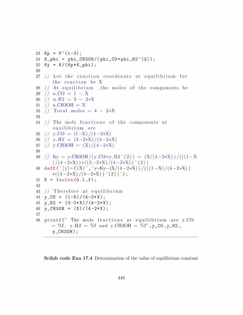
23 Kp = P^(1-3);

24 K_phi = phi_CH3OH /( phi_CO*phi_H2 ^(2));

25 Ky = K/(Kp*K_phi);

26


28 // At e q u i l i b r i u m , the moles o f the components be29 // n CO = 1 − X30 // n H2 = 3 − 2∗X31 // n CH3OH = X32 // Tota l moles = 4 − 2∗X33


35 // y CO = (1−X) /(4−2∗X)36 // y H2 = (3−2∗X) /(4−2∗X)37 // y CH3OH = (X) /(4−2∗X)38

39 // Ky = y CH3OH/( y CO∗y H2 ˆ ( 2 ) ) = (X/(4−2∗X) ) /(((1−X) /(4−2∗X) ) ∗((3−2∗X) /(4−2∗X) ) ˆ ( 2 ) )

40 deff( ’ [ y ]= f (X) ’ , ’ y=Ky−(X/(4−2∗X) ) /(((1−X) /(4−2∗X) )∗((3−2∗X) /(4−2∗X) ) ˆ ( 2 ) ) ’ );

41 X = fsolve (0.1,f);

42

43 // T h e r e f o r e at e q u i l i b r i u m44 y_CO = (1-X)/(4 -2*X);

45 y_H2 = (3-2*X)/(4-2*X);

46 y_CH3OH = (X)/(4 -2*X);

47

48 printf(” The mole f r a c t i o n s at e q u i l i b r i u m ar e y CO= %f , y H2 = %f and y CH3OH = %f”,y_CO ,y_H2 ,y_CH3OH);

Scilab code Exa 17.4 Determination of the value of equilibrium constant

448

1 clear;

2 clc;

3


8 // Given9 T = 600; // [K] − Reactor t empera tu r e10 P = 4; // [ atm ] − Reactor p r e s s u r e11 K = 1.175; // E q u i l i b r i u m c o n s t a n t12

13 // ( 1 / 2 ) ∗N2 + ( 3 / 2 ) ∗H 2 − NH314

15 // I n i t i a l number o f moles o f the components a r e16 n_N2 = 1;

17 n_H2 = 3;

18 n_HN3 = 0;

19

20 // Let the r e a c t i o n c o o r d i n a t e at e q u i l i b r i u m f o rthe r e a c t i o n be X.

21 // At e q u i l i b r i u m , the moles o f the components be22 // n N2 = 1 − 0 . 5∗X23 // n H2 = 3 − 1 . 5∗X24 // n NH3 = X25 // Tota l moles = 4 − X26

27 // We have , K = Ky∗Kp28 Kp = P^(1-2);// [ atmˆ(−1) ]29 Ky = K/(Kp);

30

31 // Ky = y NH3 /( y N2 ˆ ( 1 / 2 ) ∗y H2 ˆ ( 3 / 2 ) ) = (X/(4−X) )/( ( (1 −0 .5∗X) /(4−X) ) ˆ ( 1 / 2 ) ∗ ( (3−1 .5∗X) /(4−X) ) ˆ ( 3 / 2 ))

32 // S o l v i n g the above e q u a t i o n we g e t33 deff( ’ [ y ]= f (X) ’ , ’ y=Ky − (X/(4−X) ) /( ( (1 −0 .5∗X) /(4−X) )

ˆ ( 1 / 2 ) ∗ ( (3−1 .5∗X) /(4−X) ) ˆ ( 3 / 2 ) ) ’ );34 X = fsolve (0.1,f);

449

35

36 y_NH3 = X/(4-X);// Mole f r a c t i o n o f NH3 ate q u i l i b r i u m

37

38 printf(” The v a l u e o f Kp = %f and Ky = %f \n”,Kp ,Ky);

39 printf(” The mole f r a c t i o n s o f NH3 at e q u i l i b r i u m i s%f\n\n”,y_NH3);

40

41 // I f r e a c t i o n c a r r i e d out at c o n s t a n t t empera tu r eand volume

42

43 // We know tha t f o r i d e a l gas , P∗V = n∗R∗T and thusP i s d i r e c t l y p r o p o r t i o n a l to n at c o n s t a n t V and

T.44 // Let P = k∗n45 // I n i t i a l l y P = 4 atm and n = 4 moles , thus K = 1

and we g e t p = n , where P i s i n atm .46 // Thus at e q u i l i b r i u m P = 4 − X47

48 // Ky = K/Kp = 1 . 1 7 5∗P = 1 . 1 7 5∗ ( 4 − X)49 // (X/(4−X) ) /( ( (1 −0 .5∗X) /(4−X) ) ˆ ( 1 / 2 ) ∗ ( (3−1 .5∗X) /(4−

X) ) ˆ ( 3 / 2 ) ) = 1 . 1 7 5∗ ( 4 − X)50 // S o l v i n g the above e q u a t i o n we g e t51 deff( ’ [ y ]= f 1 (X) ’ , ’ y=(X/(4−X) ) /( ( (1 −0 .5∗X) /(4−X) )

ˆ ( 1 / 2 ) ∗ ( (3−1 .5∗X) /(4−X) ) ˆ ( 3 / 2 ) ) −1.175∗(4−X) ’ );52 X_prime = fsolve(1,f1);

53

54 // T h e r e f o r e at e q u i l i b r i u m55 P_prime = 4 - X_prime;

56 y_NH3_prime = X_prime /(4- X_prime);

57

58 printf(” I f r e a c t i o n i s c a r r i e d out at c o n s t a n tt empera tu re and volume , then \n”);

59 printf(” The e q u i l i b r i u m p r e s s u r e i s %f atm\n”,P_prime);

60 printf(” The e q u i l i b r i u m mole f r a c t i o n s o f NH3 i nthe r e a c t o r i s %f\n\n”,y_NH3_prime);

450

Scilab code Exa 17.5 Determination of mole fraction

1 clear;

2 clc;

3


8 // Given9 T = 400; // [K] − Reactor t empera tu r e10 P = 1; // [ atm ] − Reactor p r e s s u r e11 K = 1.52; // E q u i l i b r i u m c o n s t a n t12 y_H2 = 0.4; // E q u i l i b r i u m mole f r a c t i o n o f hydrogen13

14 // CO( g ) + 2∗H 2 ( g ) − CH3OH( g )15

16 // K = y CH3OH/( y CO∗y H2 ˆ ( 2 ) ∗Pˆ ( 2 ) )17 // Let t o t a l number o f moles at e q u i l i b r i u m be 118 // y CH3OH = 0 . 6 − y CO ;19 // ( 0 . 6 − y CO ) /y CO = K∗Pˆ ( 2 ) ∗y H2 ˆ ( 2 )20

21 y_CO = 0.6/(1 + K*P^(2)*y_H2 ^(2));

22 y_CH3OH = 0.6 - y_CO;

23

24 printf(” The mole f r a c t i o n s are , y CO = %f andy CH3OH = %f \n”,y_CO ,y_CH3OH);


1 clear;

451

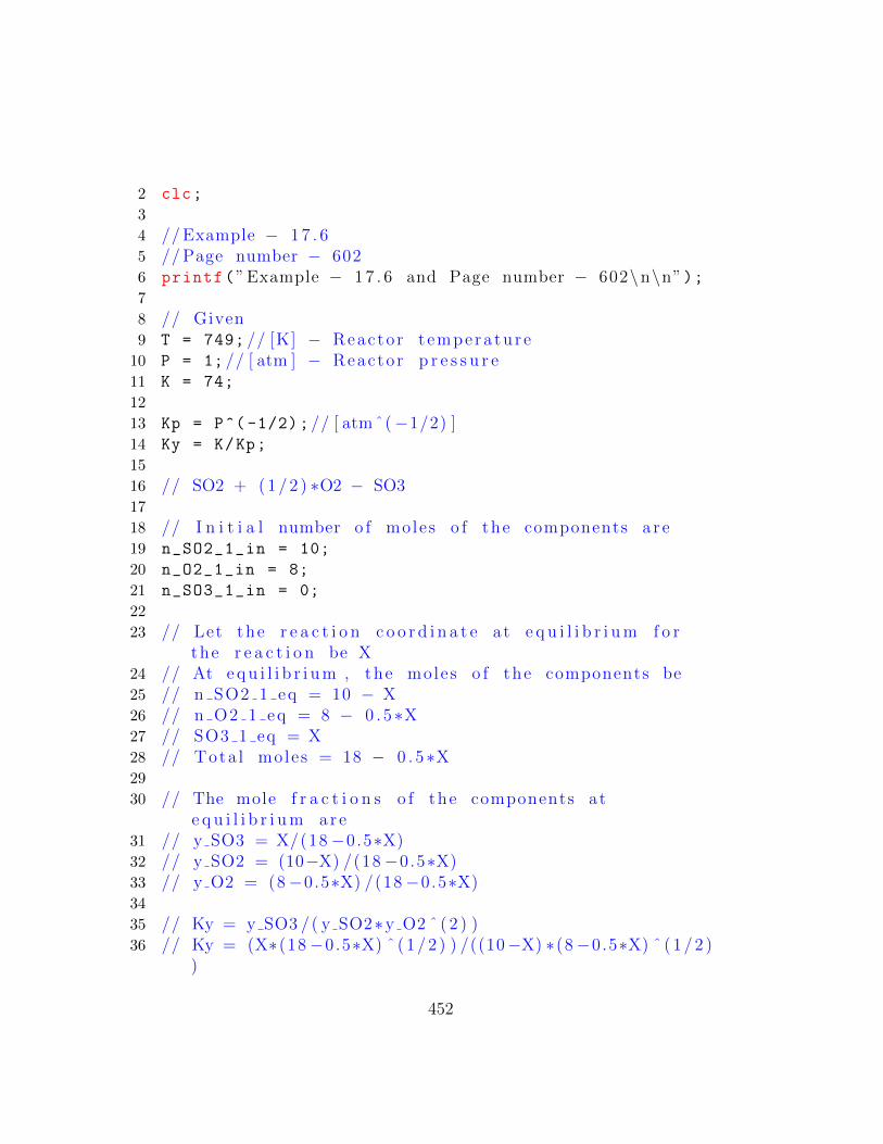
2 clc;

3


8 // Given9 T = 749; // [K] − Reactor t empera tu r e10 P = 1; // [ atm ] − Reactor p r e s s u r e11 K = 74;

12

13 Kp = P^( -1/2);// [ atmˆ(−1/2) ]14 Ky = K/Kp;

15

16 // SO2 + ( 1 / 2 ) ∗O2 − SO317

18 // I n i t i a l number o f moles o f the components a r e19 n_SO2_1_in = 10;

20 n_O2_1_in = 8;

21 n_SO3_1_in = 0;

22


24 // At e q u i l i b r i u m , the moles o f the components be25 // n SO2 1 eq = 10 − X26 // n O2 1 eq = 8 − 0 . 5∗X27 // SO3 1 eq = X28 // Tota l moles = 18 − 0 . 5∗X29


31 // y SO3 = X/(18−0.5∗X)32 // y SO2 = (10−X) /(18−0.5∗X)33 // y O2 = (8−0.5∗X) /(18−0.5∗X)34

35 // Ky = y SO3 /( y SO2∗y O2 ˆ ( 2 ) )36 // Ky = (X∗(18−0.5∗X) ˆ ( 1 / 2 ) ) /((10−X) ∗(8−0.5∗X) ˆ ( 1 / 2 )

)

452

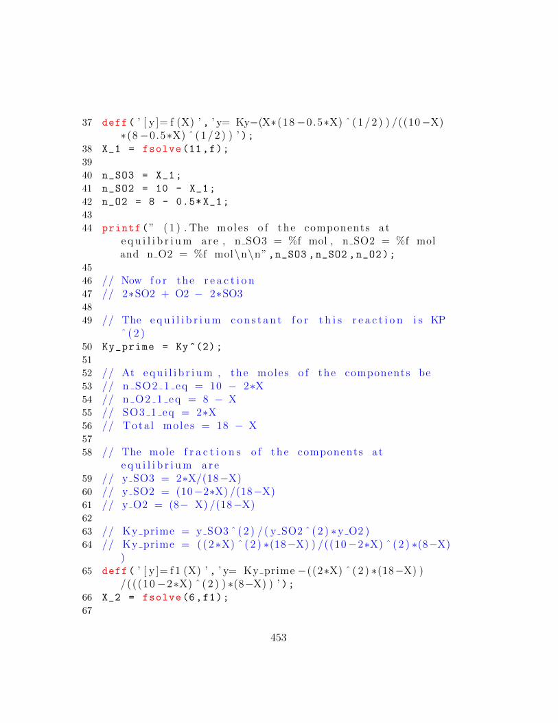
37 deff( ’ [ y ]= f (X) ’ , ’ y= Ky−(X∗(18−0.5∗X) ˆ ( 1 / 2 ) ) /((10−X)∗(8−0.5∗X) ˆ ( 1 / 2 ) ) ’ );

38 X_1 = fsolve (11,f);

39

40 n_SO3 = X_1;

41 n_SO2 = 10 - X_1;

42 n_O2 = 8 - 0.5* X_1;

43

44 printf(” ( 1 ) . The moles o f the components ate q u i l i b r i u m are , n SO3 = %f mol , n SO2 = %f moland n O2 = %f mol\n\n”,n_SO3 ,n_SO2 ,n_O2);

45

46 // Now f o r the r e a c t i o n47 // 2∗SO2 + O2 − 2∗SO348

49 // The e q u i l i b r i u m c o n s t a n t f o r t h i s r e a c t i o n i s KPˆ ( 2 )

50 Ky_prime = Ky^(2);

51

52 // At e q u i l i b r i u m , the moles o f the components be53 // n SO2 1 eq = 10 − 2∗X54 // n O2 1 eq = 8 − X55 // SO3 1 eq = 2∗X56 // Tota l moles = 18 − X57


59 // y SO3 = 2∗X/(18−X)60 // y SO2 = (10−2∗X) /(18−X)61 // y O2 = (8− X) /(18−X)62

63 // Ky prime = y SO3 ˆ ( 2 ) /( y SO2 ˆ ( 2 ) ∗y O2 )64 // Ky prime = ( ( 2∗X) ˆ ( 2 ) ∗(18−X) ) /((10−2∗X) ˆ ( 2 ) ∗(8−X)

)65 deff( ’ [ y ]= f 1 (X) ’ , ’ y= Ky prime −((2∗X) ˆ ( 2 ) ∗(18−X) )

/(((10−2∗X) ˆ ( 2 ) ) ∗(8−X) ) ’ );66 X_2 = fsolve(6,f1);

67

453

68 n_SO3_prime = 2*X_2;

69 n_SO2_prime = 10 - 2*X_2;

70 n_O2_prime = 8 - X_2;

71

72 printf(” ( 2 ) . The moles o f the components ate q u i l i b r i u m are , n SO3 = %f mol , n SO2 = %f moland n O2 = %f mol\n\n”,n_SO3_prime ,n_SO2_prime ,n_O2_prime);

73 printf(” Thus the number o f moles r ema ins thesame i r r e s p e c t i v e o f the s t o i c h o i m e t r y o f ther e a c t i o n ”)

Scilab code Exa 17.7 Calculation of mole fraction

1 clear;

2 clc;

3


8 // Given9 T = 500; // [K]10 // For the r e a c t i o n , 0 . 5∗A2 + 0 . 5∗B2 − AB11 delta_G = -4200; // [ J/mol ]12 R = 8.314; // [ J/mol∗K] − U n i v e r s a l gas c o n s t a n t13

14 // ( 1 )15 // A2 + B2 − 2∗AB16

17 // We know d e l t a G r k n 0 = −R∗T∗ l o g (K)18 delta_G_1 = 2* delta_G;

19 K_1 = exp(-delta_G_1 /(R*T));// E q u i l i b r i u m c o n s t a n tat 500 K f o r the above r e a c t i o n

20 // As can be s e en the r e a c t i o n i s not a f f e c t e d by

454

p r e s s u r e and t h e r e f o r e K = Ky as Kp = 121 Ky = K_1;

22

23 // I n i t i a l number o f moles o f the components a r e24 n_A2_1_in = 0.5;

25 n_B2_1_in = 0.5;

26 n_AB_1_in = 0;

27


29 // At e q u i l i b r i u m , the moles o f the components be30 // n A2 1 eq = 0 . 5 − X31 // n B2 1 eq = 0.5− X32 // n AB 1 eq = 2∗X33 // Tota l moles = 134

35 // Ky = (2∗X) ˆ ( 2 ) /(0.5−X) ˆ ( 2 )36 deff( ’ [ y ]= f (X) ’ , ’ y= Ky−(2∗X) ˆ ( 2 ) /(0.5−X) ˆ ( 2 ) ’ );37 X_1 = fsolve (0.2,f);

38


40 y_A2_1 = 0.5 - X_1;

41 y_B2_1 = 0.5- X_1;

42 y_AB_1 = 2*X_1;

43

44 printf(” ( 1 ) . The mole f r a c t i o n s at e q u i l i b r i u m a r ey A2 = %f , y B2 = %f and y AB = %f\n\n”,y_A2_1 ,y_B2_1 ,y_AB_1);

45

46 // ( 2 )47 // 0 . 5∗A2 + 0 . 5∗B2 − AB48

49 // We know d e l t a G r k n 0 = −R∗T∗ l o g (K)50 delta_G_2 = delta_G;

51 K_2 = exp(-delta_G_2 /(R*T));// E q u i l i b r i u m c o n s t a n tat 500 K f o r the above r e a c t i o n

52

455

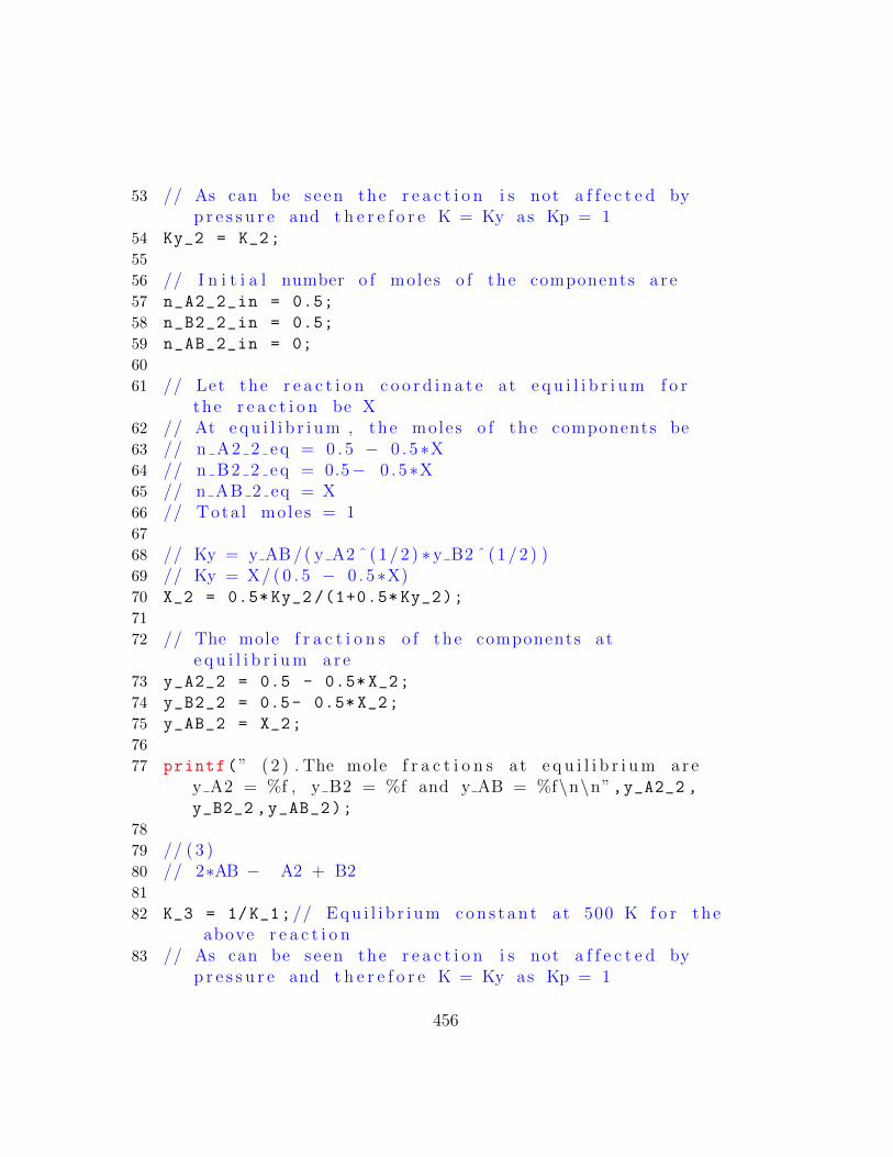
53 // As can be s e en the r e a c t i o n i s not a f f e c t e d byp r e s s u r e and t h e r e f o r e K = Ky as Kp = 1

54 Ky_2 = K_2;

55

56 // I n i t i a l number o f moles o f the components a r e57 n_A2_2_in = 0.5;

58 n_B2_2_in = 0.5;

59 n_AB_2_in = 0;

60


62 // At e q u i l i b r i u m , the moles o f the components be63 // n A2 2 eq = 0 . 5 − 0 . 5∗X64 // n B2 2 eq = 0.5− 0 . 5∗X65 // n AB 2 eq = X66 // Tota l moles = 167

68 // Ky = y AB /( y A2 ˆ ( 1 / 2 ) ∗y B2 ˆ ( 1 / 2 ) )69 // Ky = X/ ( 0 . 5 − 0 . 5∗X)70 X_2 = 0.5* Ky_2 /(1+0.5* Ky_2);

71


73 y_A2_2 = 0.5 - 0.5* X_2;

74 y_B2_2 = 0.5- 0.5* X_2;

75 y_AB_2 = X_2;

76


78

79 // ( 3 )80 // 2∗AB − A2 + B281

82 K_3 = 1/K_1;// E q u i l i b r i u m c o n s t a n t at 500 K f o r theabove r e a c t i o n

83 // As can be s e en the r e a c t i o n i s not a f f e c t e d byp r e s s u r e and t h e r e f o r e K = Ky as Kp = 1

456

84 Ky_3 = K_3;

85

86 // I n i t i a l number o f moles o f the components a r e87 n_AB_3_in = 1;

88 n_A2_3_in = 0;

89 n_B2_3_in = 0;

90


92 // At e q u i l i b r i u m , the moles o f the components be93 // n AB 3 eq = 1 − X94 // n A2 3 eq = X/295 // n B2 3 eq = X/296 // Tota l moles = 197

98 // Ky = (X/2) ˆ ( 2 ) /(1−X) ˆ ( 2 )99 deff( ’ [ y ]= f 1 (X) ’ , ’ y= Ky 3−(X/2) ˆ ( 2 ) /(1−X) ˆ ( 2 ) ’ );

100 X_3 = fsolve (0.4,f1);

101


103 y_A2_3 = X_3/2;

104 y_B2_3 = X_3/2;

105 y_AB_3 = 1-X_3;

106


Scilab code Exa 17.8 Calculation of heat exchange

1 clear;

2 clc;

3

4 // Example − 1 7 . 8

457


8 // Given9 // P∗P +q∗Q − r ∗R + s ∗S10 // Let Cp P = p , Cp Q = Q, Cp R = R and Cp S = S11

12 // ( 1 )13 // When r e a c t a n t s a r e heated from 10 to 25 C,

r e a c t i o n t a k e s p l a c e at 25 C and p r o d u c t s a r er a i s e d from 25 C to 1500 K the heat exchange i sg i v e n by

14 T_1 = 10 + 273.15; // [K]15 T_2 = 25 + 273.15; // [K]16 T_3 = 1500; // [K]17 // Q = i n t e g r a t e ( ’ ( p∗Cp P + q∗Cp q ) ∗dT ’ , ’ T’ , T 1 , T 2 )

+ d e l t a H r k n 2 9 8 + i n t e g r a t e ( ’ ( r ∗Cp R + s ∗Cp S )∗dT ’ , ’ T’ T 2 , T 3 ) ;

18 printf(” ( 1 ) . The e x p r e s s i o n f o r the heat exchangewith the s u r r o u n d i n g by the f i r s t path i s g i v e nbelow \n”);

19 printf(” Q = i n t e g r a t e ( ( p∗Cp P + q∗Cp q ) ∗dT , T,T 1 , T 2 ) + d e l t a H r k n 2 9 8 + i n t e g r a t e ( ( r ∗Cp R +s ∗Cp S ) ∗dT , TT 2 , T 3 ) ; \ n\n”)

20

21 // ( 2 )22 // When r e a c t a n t s a r e heated from 10 C to 1500 K,

r e a c t i o n take p l a c e at 1500 K the heat exchangei s g i v e n by

23 // Q = i n t e g r a t e ( ’ ( p∗Cp P + q∗Cp q ) ∗dT ’ , ’ T’ , T 1 , T 3 )+ d e l t a H r k n 1 5 0 0

24 // where , d e l t a H r k n 1 5 0 0 = d e l t a H r k n 2 9 8 +i n t e g r a t e ( ’ ( r ∗Cp R + s ∗Cp S − p∗Cp P − q∗Cp q ) ∗dT’ , ’ T’ T 2 , T 3 ) ;

25 // T h e r e f o r e26 // Q = i n t e g r a t e ( ’ ( p∗Cp P + q∗Cp q ) ∗dT ’ , ’ T’ , T 1 , T 3 )

+ d e l t a H r k n 2 9 8 + i n t e g r a t e ( ’ ( r ∗Cp R + s ∗Cp S− p∗Cp P − q∗Cp q ) ∗dT ’ , ’ T’ T 2 , T 3 ) ;

458

27 // Q = i n t e g r a t e ( ’ ( p∗Cp P + q∗Cp q ) ∗dT ’ , ’ T’ , T 1 , T 2 )+ d e l t a H r k n 2 9 8 + i n t e g r a t e ( ’ ( r ∗Cp R + s ∗Cp S )∗dT ’ , ’ T’ T 2 , T 3 ) ;

28

29 // which i s same as i n method ( 1 ) . The t o t a len tha lpy change between two f i x e d ponts i s af u n c t i o n on ly o f s t a t e and not the path taken .

30

31 printf(” ( 2 ) . The e x p r e s s i o n f o r the heat exchangewith the s u r r o u n d i n g by the second path i s g i v e nbelow \n”);

32 printf(” Q = i n t e g r a t e ( ( p∗Cp P + q∗Cp q ) ∗dT , T,T 1 , T 2 ) + d e l t a H r k n 2 9 8 + i n t e g r a t e ( ( r ∗Cp R +s ∗Cp S ) ∗dT , TT 2 , T 3 ) ; \ n\n”)

Scilab code Exa 17.9 Dtermination of heat of reaction

1 clear;

2 clc;

3


8 // Given9 // SO2 + ( 1 / 2 ) ∗O2 − SO310 R = 1.987; // [ c a l /mol−K]11

12 delta_H_SO2_298 = -70.96; // [ k c a l /mol ] − Enthalpy o ff o r m a t i o n o f S02 at 2 9 8 . 1 5 K

13 delta_H_SO3_298 = -94.45; // [ k c a l /mol ] − Enthalpy o ff o r m a t i o n o f S03 at 2 9 8 . 1 5 K

14 delta_G_SO2_298 = -71.79; // [ k c a l /mol ] − Gibbs f r e eene rgy change f o r f o r m a t i o n o f SO2 at 2 9 8 . 1 5 K

15 delta_G_SO3_298 = -88.52; // [ k c a l /mol ] − Gibbs f r e e

459

ene rgy change f o r f o r m a t i o n o f SO3 at 2 9 8 . 1 5 K16

17 // Cp 0 = a + b∗T + c ∗Tˆ ( 2 ) + d∗Tˆ ( 3 )18

19 a_SO2 = 6.157;

20 a_SO3 = 3.918;

21 a_O2 = 6.085;

22 b_SO2 = 1.384*10^( -2);

23 b_SO3 = 3.483*10^( -2);

24 b_O2 = 0.3631*10^( -2);

25 c_SO2 = -0.9103*10^( -5);

26 c_SO3 = -2.675*10^( -5);

27 c_O2 = -0.1709*10^( -5);

28 d_SO2 = 2.057*10^( -9);

29 d_SO3 = 7.744*10^( -9);

30 d_O2 = 0.3133*10^( -9);

31

32 // ( 1 )33 T_1 = 298.15; // [K]34

35 delta_H_rkn_298 = delta_H_SO3_298 - delta_H_SO2_298;

// [ k c a l ]36 delta_H_rkn_298 = delta_H_rkn_298 *10^(3);// [ c a l ]37 delta_G_rkn_298 = delta_G_SO3_298 - delta_G_SO2_298;

// [ k c a l ]38 delta_G_rkn_298 = delta_G_rkn_298 *10^(3);// [ c a l ]39

40 delta_a = a_SO3 - a_SO2 - (a_O2 /2);

41 delta_b = b_SO3 - b_SO2 - (b_O2 /2);

42 delta_c = c_SO3 - c_SO2 - (c_O2 /2);

43 delta_d = d_SO3 - d_SO2 - (d_O2 /2);

44

45 // d e l t a H r k n T = d e l t a H r k n 2 9 8 + i n t e g r a t e ( ’d e l t a a +( d e l t a b ∗T) +( d e l t a c ∗Tˆ ( 2 ) ) +( d e l t a d ∗Tˆ ( 3 ) ) ’ , ’T’ , T 1 ,T) ;

46 // On s i m p l i f i c a t i o n we ge t47 // d e l t a H r k n T = −22630.14 − 5 . 2 8 1 5∗T +

0.9587∗10ˆ( −2) ∗Tˆ ( 2 ) − 0 .5598∗10ˆ( −5) ∗Tˆ ( 3 ) +

460

1 .3826∗10ˆ( −9) ∗Tˆ ( 4 )48

49 printf(” ( 1 ) . The e x p r e s s i o n f o r d e l t a H r k n T as af u n c t i o n o f T i s g i v e n by\n”);

50 printf(” d e l t a H r k n T = −22630.14 − 5 . 2 8 1 5∗T +0.9587∗10ˆ( −2) ∗Tˆ ( 2 ) − 0 .5598∗10ˆ( −5) ∗Tˆ ( 3 ) +1.3826∗10ˆ( −9) ∗Tˆ ( 4 ) \n\n”);

51

52 // ( 2 )53 // R∗ l o g (K T/ K 298 ) = i n t e g r a t e ( ’ d e l t a H r k n T /Tˆ ( 2 )

’ ,T, T 1 ,T)54 // F i r s t l e t us c a l c u l a t e K 298 .55 // d e l t a G r k n T = − R∗T∗ l o g (K)56 K_298 = exp(-delta_G_rkn_298 /(R*T_1));

57

58 // On s u b s t i t u t i n g the v a l u e s and s i m p l i f y i n g we g e tthe e x p r e s s i o n

59 // l o g (K) = 3 . 8 7 + 1 1 3 80 . 1 0 /T − 2 . 6 5 8 0∗ l o g (T) +0.4825∗10ˆ( −2) ∗T − 0 .1409∗10ˆ( −5) ∗Tˆ ( 2 ) +0.2320∗10ˆ( −9) ∗Tˆ ( 3 )

60

61 printf(” ( 2 ) . The e x p r e s s i o n f o r l o g (K) as a f u n c t i o no f T i s g i v e n by\n”);

62 printf(” l o g (K) = 3 . 8 7 + 1 1 3 8 0 . 10 /T − 2 . 6 5 8 0∗ l o g(T) + 0.4825∗10ˆ( −2) ∗T − 0 .1409∗10ˆ( −5) ∗Tˆ ( 2 ) +0.2320∗10ˆ( −9) ∗Tˆ ( 3 ) \n\n”);

63

64 // ( 3 )65 P = 1; // [ atm ]66 T = 880; // [K]67 K = exp (3.87 + 11380.10/T - 2.6580* log(T) +

0.4825*10^( -2)*T - 0.1409*10^( -5)*T^(2) +

0.2320*10^( -9)*T^(3));

68 Kp = P^( -1/2);// [ atmˆ(−1/2) ]69 Ky = K/Kp;

70


461

72 // At e q u i l i b r i u m , the moles o f the components be73 // n SO2 eq = 1 − X74 // n O2 eq = 0.5− 0 . 5∗X75 // n SO3 1 eq = X76 // Tota l moles = 1.5−0 .5∗X77

78 // Ky = (X∗ (1 .5 −0 .5∗X) ˆ ( 1 / 2 ) ) /((1−X) ∗ (0 .5 −0 .5∗X)ˆ ( 1 / 2 ) )

79 deff( ’ [ y ]= f (X) ’ , ’ y= Ky − (X∗ (1 . 5 −0 .5∗X) ˆ ( 1 / 2 ) ) /((1−X) ∗ (0 .5 −0 .5∗X) ˆ ( 1 / 2 ) ) ’ );

80 X = fsolve (0.8,f);

81

82 // The mole f r a c t i o n o f SO3 at e q u i l i b r i u m i s g i v e nby

83 y_SO3 = X/(1.5 -0.5*X);

84

85 printf(” ( 3 ) . The mole f r a c t i o n o f SO3 at e q u i l i b r i u mi s g i v e n by , y SO3 = %f\n”,y_SO3);

Scilab code Exa 17.10 Tabulation of equilibrium constant values

1 clear;

2 clc;

3


8 // Given9 // ( 1 / 2 ) ∗N2 + ( 1 / 2 ) ∗O2 − NO10

11 R = 1.987; // [ c a l /mol−K]12

13 delta_H_NO_298 = 21.600; // [ k c a l /mol ] − Enthalpy o ff o r m a t i o n o f S02 at 2 9 8 . 1 5 K

462

14 delta_G_NO_298 = 20.719; // [ k c a l /mol ] − Gibbs f r e eene rgy change f o r f o r m a t i o n o f SO2 at 2 9 8 . 1 5 K

15

16 // Cp 0 = a + b∗T + c ∗Tˆ ( 2 ) + d∗Tˆ ( 3 )17

18 a_N2 = 6.157;

19 a_O2 = 6.085;

20 a_NO = 6.461;

21 b_N2 = -0.03753*10^( -2);

22 b_O2 = 0.3631*10^( -2);

23 b_NO = 0.2358*10^( -2);

24 c_N2 = 0.1930*10^( -5);

25 c_O2 = -0.1709*10^( -5);

26 c_NO = -0.07705*10^( -5);

27 d_N2 = -0.6861*10^( -9);

28 d_O2 = 0.3133*10^( -9);

29 d_NO = 0.08729*10^( -9);

30

31 // ( 1 )32 T_1 = 298.15; // [K]33

34 delta_H_rkn_298 = delta_H_NO_298;// [ k c a l ]35 delta_H_rkn_298 = delta_H_rkn_298 *10^(3);// [ c a l ]36 delta_G_rkn_298 = delta_G_NO_298;// [ k c a l ]37 delta_G_rkn_298 = delta_G_rkn_298 *10^(3);// [ c a l ]38

39 delta_a = a_NO - (a_N2 /2) - (a_O2 /2);

40 delta_b = b_NO - (b_N2 /2) - (b_O2 /2);

41 delta_c = c_NO - (c_N2 /2) - (c_O2 /2);

42 delta_d = d_NO - (d_N2 /2) - (d_O2 /2);

43


45 // On s i m p l i f i c a t i o n we ge t46 // d e l t a H r k n T = 2 1 5 8 4 . 6 3 − 0 . 0 3 3∗T +

0.0365∗10ˆ( −2) ∗Tˆ ( 2 ) − 0 .0293∗10ˆ( −5) ∗Tˆ ( 3 ) +0.0685∗10ˆ( −9) ∗Tˆ ( 4 )

463

47

48 printf(” The e x p r e s s i o n f o r d e l t a H r k n T as af u n c t i o n o f T i s g i v e n by\n”);

49 printf(” d e l t a H r k n T = 2 1 5 8 4 . 6 3 − 0 . 0 3 3∗T +0.0365∗10ˆ( −2) ∗Tˆ ( 2 ) − 0 .0293∗10ˆ( −5) ∗Tˆ ( 3 ) +0.0685∗10ˆ( −9) ∗Tˆ ( 4 ) \n\n”);

50

51 // Now l e t us c a l c u l a t e K 298 ( at 298 K)52 // We know d e l t a G r k n 2 9 8 = −R∗T∗ l o g ( K 298 )53 K_298 = exp(-delta_G_rkn_298 /(R*T_1));// E q u i l i b r i u m

c o n s t a n t at 2 9 8 . 1 5 K54

55 // l o g ( K 2/K 1 ) = i n t e g r a t e ( ’ d e l t a H r k n 2 9 8 /(R∗Tˆ ( 2 ) ) ’ , ’T’ , T 1 ,T)

56 // On s u b s t i t u t i n g the v a l u e s and s i m p l i f y i n g we g e tthe e x p r e s s i o n

57 // l o g (K) = 1 . 5 1 0 3 − 1 0 8 62 . 9 2 /T − 0 . 0 1 6 6∗ l o g (T) +1.84∗10ˆ( −4) ∗T − 7 .35∗10ˆ( −8) ∗Tˆ ( 2 ) +1.15∗10ˆ( −11) ∗Tˆ ( 3 )

58

59 printf(” The e x p r e s s i o n f o r l o g (K) as a f u n c t i o n o fT i s g i v e n by\n”);

60 printf(” l o g (K) = 1 . 5 1 0 3 − 1 0 8 6 2 . 9 2 /T − 0 . 0 1 6 6∗ l o g (T) + 1.84∗10ˆ( −4) ∗T − 7 .35∗10ˆ( −8) ∗Tˆ ( 2 ) +1.15∗10ˆ( −11) ∗Tˆ ( 3 ) \n\n\n\n”)

61

62 T = [500 ,1000 ,1500 ,2000 ,2500];

63 K = zeros (5);

64

65 printf(” T (K) \ t \ t \ t K \n\n”);66

67 for i=1:5;

68 K(i) = exp (1.5103 -10862.92/T(i) - 0.0166* log(T(i

)) + 1.84*10^( -4)*T(i) - 7.35*10^( -8)*T(i)

^(2) + 1.15*10^( -11)*T(i)^(3));

69

70 printf(” %f \ t \ t %e \n\n”,T(i),K(i));71 end

464

72


75 // I t can be s e en tha t f o r endothermic r e a c t i o n se q u i l i b r i u m c o n s t a n t i n c r e a s e s with t empera tu r e .

76 printf(” I t can be s e en tha t f o r endothe rmicr e a c t i o n s e q u i l i b r i u m c o n s t a n t i n c r e a s e s witht empera tu re \n”);

Scilab code Exa 17.11 Determination of mean standard enthalpy of reac-tion

1 clear;

2 clc;

3


8 // Given9 // SO2 + ( 1 / 2 ) ∗O2 − SO310 R = 8.314; // [ J/mol−K]11

12 K_800 = 0.0319; // E q u i l i b r i u m c o n s t a n t at 800 K13 K_900 = 0.153; // E q u i l i b r i u m c o n s t a n t at 900 K14 T_1 = 800; // [K]15 T_2 = 900; // [K]16

17 // We have the r e l a t i o n18 // l o g ( K 2/K 1 ) = −( d e l t a H r k n /R) ∗ (1/ T 2 − 1/ T 1 )19 // l o g ( K 900 / K 800 ) = −( d e l t a H r k n 8 5 0 /R) ∗ (1/ T 2 −

1/ T 1 )20 delta_H_rkn_850 = -R*log(K_900/K_800)/(1/ T_2 - 1/T_1

);// [ J ]21 delta_H_rkn_850 = delta_H_rkn_850 *10^( -3);// [ kJ ]

465

22

23 printf(” The mean s tandard en tha lpy change o fr e a c t i o n i n the r e g i o n 800 t0 900 i s g i v e n byd e l t a H r k n 8 5 0 = %f \n”,delta_H_rkn_850);

Scilab code Exa 17.12 Derivation of expression for enthalpy of reaction

1 clear;

2 clc;

3


8 // Given9 // l o g (K) = −2.61 + 2 3 67 2 . 6 2 /T − 7 . 1 7∗ l o g (T) +

1.24∗10ˆ( −2) ∗T − 0 .148∗10ˆ( −5) ∗Tˆ ( 2 ) +0.039∗10ˆ( −9) ∗Tˆ ( 3 )

10

11 // We know tha t12 // d l og (K) /dT = d e l t a H r k n /(R∗Tˆ ( 2 ) )13

14 // D i f f e r e n t i a t i n g the above e x p r e s s i o n o f l o g (K) , weg e t

15 // d l og (K) /dT = −23672.62/Tˆ ( 2 ) − 7 . 1 7 /T +1.24∗10ˆ( −2) − 2∗0 .148∗10ˆ( −5) ∗T +3∗0 .039∗10ˆ( −9) ∗Tˆ ( 2 )

16

17 // On f u r t h e r s i m p l i f i c a t i o n we g e t18 // d e l t a H r k n = −47037.5 − 1 4 . 2 4∗T + 2.46∗10ˆ( −2) ∗T

ˆ ( 2 ) − 0 .59∗10ˆ( −5) ∗Tˆ ( 3 ) + 0.23∗10ˆ( −9) ∗Tˆ ( 4 )19 printf(” d e l t a H r k n = −47037.5 − 1 4 . 2 4∗T +

2.46∗10ˆ( −2) ∗Tˆ ( 2 ) − 0 .59∗10ˆ( −5) ∗Tˆ ( 3 ) +0.23∗10ˆ( −9) ∗Tˆ ( 4 ) \n”);

466


1 clear;

2 clc;

3


8 // Given9 T_1 = 298.15; // [K]10 T = 2600; // [K]11 R = 1.987; // [ c a l /mol−K] − U n i v e r s a l gas c o n s t a n t12

13 // Cp 0 = a + b∗T + c ∗Tˆ ( 2 ) + d∗Tˆ ( 3 )14 delta_H_CO_298 = -26.416; // [ k c a l /mol ] − Enthalpy o f

f o r m a t i o n o f CO at 2 9 8 . 1 5 K15 delta_G_CO_298 = -32.808; // [ k c a l /mol ] − Gibbs f r e e

ene rgy change f o r f o r m a t i o n o f CO at 2 9 8 . 1 5 K16 delta_H_CO2_298 = -94.052; // [ k c a l /mol ] − Enthalpy o f

f o r m a t i o n o f C02 at 2 9 8 . 1 5 K17 delta_G_CO2_298 = -94.260; // [ k c a l /mol ] − Gibbs f r e e

ene rgy change f o r f o r m a t i o n o f CO2 at 2 9 8 . 1 5 K18

19 // CO + ( 1 / 2 ) ∗O2 − CO220

21 a_CO = 6.726;

22 a_O2 = 6.0685;

23 a_CO2 = 5.316;

24 b_CO = 0.04001*10^( -2);

25 b_O2 = 0.3631*10^( -2);

26 b_CO2 = 1.4285*10^( -2);

27 c_CO = 0.1283*10^( -5);

28 c_O2 = -0.1709*10^( -5);

467

29 c_CO2 = -0.8362*10^( -5);

30 d_CO = -0.5307*10^( -9);

31 d_O2 = 0.3133*10^( -9);

32 d_CO2 = 1.784*10^( -9);

33

34

35 delta_H_rkn_298 = delta_H_CO2_298 - delta_H_CO_298;

// [ k c a l ]36 delta_H_rkn_298 = delta_H_rkn_298 *10^(3);// [ c a l ]37 delta_G_rkn_298 = delta_G_CO2_298 - delta_G_CO_298;

// [ k c a l ]38 delta_G_rkn_298 = delta_G_rkn_298 *10^(3);// [ c a l ]39

40 delta_a = a_CO2 - (a_CO) - (a_O2 /2);

41 delta_b = b_CO2 - (b_CO) - (b_O2 /2);

42 delta_c = c_CO2 - (c_CO) - (c_O2 /2);

43 delta_d = d_CO2 - (d_CO) - (d_O2 /2);

44


46 // On s i m p l i f i c a t i o n we ge t47 delta_H_rkn_T = -66773.56 - 4.45*T + 0.605*10^( -2)*T

^(2) - 0.29*10^( -5)*T^(3) + 0.54*10^( -9)*T^(4);

48

49 // l o g (K/ K 298 ) = i n t e g r a t e ( ’ d e l t a H r k n T /(R∗Tˆ ( 2 ) )’ , ’T’ , T 1 ,T)

50

51 // We know tha t d e l t a G r k n T = −R∗T∗ l o g (K)52 // At 2 9 8 . 1 5 K53 K_298 = exp(-delta_G_rkn_298 /(R*T_1) );

54

55 // T h e r f o r e on s i m p l i f i c a t i o n we g e t56 // l o g (K) = 2 . 9 4 + 3 3 6 0 5 . 2 /T − 2 . 2 4∗ l o g (T) +

0.304∗10( −2) ∗T − 0 .073∗10ˆ( −5) ∗Tˆ ( 2 ) +0.09∗10ˆ( −9) ∗Tˆ ( 3 )

57 K = exp (2.94 + 33605.2/T - 2.24* log(T) +

0.304*10^( -2)*T - 0.073*10^( -5)*T^(2) +

468

0.09*10^( -9)*T^(3));

58

59 printf(” The v a l u e o f e q u i l i b r i u m c o n s t a n t at 2600K i s g i v e n by , K 298 = %f\n\n”,K);

60

61

62 // ( a )63 P_1 = 1; // [ atm ]64 Kp_1 = P_1 ^( -1/2);

65 Ky_1 = K/Kp_1;

66


68 // At e q u i l i b r i u m , the moles o f the components be69 // n CO 1 eq = 1 − X70 // n 0 2 1 e q = 0.5− 0 . 5X71 // n CO2 1 eq = X72 // Tota l moles = 1 . 5 − 0 . 5∗X73

74 // Ky = y CO2 /( y CO ˆ ( 1 / 2 ) ∗y CO )75 // ky = (X∗ (1 . 5 −0 .5∗X) ˆ ( 1 / 2 ) ) /((1−X) ∗ (0 . 5 −0 .5∗X)

ˆ ( 1 / 2 ) )76

77 deff( ’ [ y ]= f (X) ’ , ’ y= Ky 1−(X∗ (1 . 5 −0 .5∗X) ˆ ( 1 / 2 ) ) /((1−X) ∗ (0 .5 −0 .5∗X) ˆ ( 1 / 2 ) ) ’ );

78 X_1 = fsolve (0.9,f);

79

80 y_CO2_1 = X_1 /(1.5 -0.5* X_1);

81 y_CO_1 = (1-X_1)/(1.5 -0.5* X_1);

82 y_O2_1 = (0.5 -0.5* X_1)/(1.5 -0.5* X_1);

83

84 printf(” ( a ) . The e q u i l i b r i u m c o m p o s i t i o n ( at 1 atm )i s g i v e n by , y CO2 = %f , y CO = %f and y O2 = %f\n\n”,y_CO2_1 ,y_CO_1 ,y_O2_1);

85

86 // ( b )87 P_2 = 10; // [ atm ]88 Kp_2 = P_2 ^( -1/2);

469

89 Ky_2 = K/Kp_2;

90


ˆ ( 1 / 2 ) )93

94 deff( ’ [ y ]= f 1 (X) ’ , ’ y= Ky 2−(X∗ (1 .5 −0 .5∗X) ˆ ( 1 / 2 ) ) /((1−X) ∗ (0 .5 −0 .5∗X) ˆ ( 1 / 2 ) ) ’ );

95 X_2 = fsolve (0.9,f1);

96

97 y_CO2_2 = X_2 /(1.5 -0.5* X_2);

98 y_CO_2 = (1-X_2)/(1.5 -0.5* X_2);

99 y_O2_2 = (0.5 -0.5* X_2)/(1.5 -0.5* X_2);

100

101 printf(” ( b ) . The e q u i l i b r i u m c o m p o s i t i o n ( at 10 atm )i s g i v e n by , y CO2 = %f , y CO = %f and y O2 = %f\n\n”,y_CO2_2 ,y_CO_2 ,y_O2_2);

102

103 // ( c )104 P_3 = 1; // [ atm ]105 Kp_3 = P_3 ^( -1/2);

106 Ky_3 = K/Kp_3;

107


ˆ ( 1 / 2 ) )110

111 // At e q u i l i b r i u m , the moles o f the components be112 // n CO 3 eq = 1 − X113 // n 0 2 3 e q = 0.5− 0 . 5X114 // n CO2 3 eq = X115 // n N2 eq = 1 ;116 // Tota l moles = 2 . 5 − 0 . 5∗X117

118 deff( ’ [ y ]= f 2 (X) ’ , ’ y= Ky 3−(X∗ (2 .5 −0 .5∗X) ˆ ( 1 / 2 ) ) /((1−X) ∗ (0 .5 −0 .5∗X) ˆ ( 1 / 2 ) ) ’ );

119 X_3 = fsolve (0.9,f2);

120

470

121 y_CO2_3 = X_3 /(2.5 -0.5* X_3);

122 y_CO_3 = (1-X_3)/(2.5 -0.5* X_3);

123 y_O2_3 = (0.5 -0.5* X_3)/(2.5 -0.5* X_3);

124 y_N2 = 1/(2.5 -0.5* X_3);

125

126 printf(” ( c ) . The e q u i l i b r i u m c o m p o s i t i o n ( at 1 atmand 1 mol N2) i s g i v e n by , y CO2 = %f , y CO = %f, y O2 = %f and y N2 = %f\n\n”,y_CO2_3 ,y_CO_3 ,y_O2_3 ,y_N2);


1 clear;

2 clc;

3


8 // Given9 T = 25 + 298.15; // [K] − Temperature10 R = 8.314; // [ J/mol−K]11 delta_G_298 = -1000; // [ J ] − Gibbs f r e e ene rgy change

at 298 K12

13 // G E /(R∗T) = x 1 ∗ x 214

15 // We know tha t d e l t a G r k n = − R∗T∗ l o g (K) ,t h e r e f o r e

16 K = exp(-delta_G_298 /(R*T));

17

18 // ( 1 )19 // Let x 1 i s the mole f r a c t i o n o f A and x 2 be the

mole f r a c t i o n o f B20 // I f A and B form an i d e a l mixture then ,

471

21 Ky = 1;

22 // and K = Kx = x 2 / x 123 // and at e q u i l i b r i u m x 2 / x 1 = K24 // (1− x 1 ) / x 1 = K25 x_1 = 1/(1+K);

26

27 printf(” ( 1 ) . The e q u i l i b r i u m c o m p o s i t i o n ( f o r i d e a lb ehav i ou r ) i s g i v e n by x 1 = %f\n\n”,x_1);

28

29 // ( 2 )30 // The a c t i v i t y c o e f f i c i e n t s a r e g i v e n by31 // l o g (Y1) = [ d e l ( n∗G E /(R∗T) ) / d e l ( n 1 ) ] T , P , n 2 =

x 2 ˆ ( 2 )32 // s i m i l a r l y , l o g (Y2) = x 1 ˆ ( 2 )33

34 // The e q u i l i b r i u m c o n s t a n t f o r the l i q u i d phaser e a c t i o n i s g i v e n by

35 // K = Kx∗Ky = ( x 2 ∗Y2) /( x 1 ∗Y1) = ( x 2 ∗ exp ( x 1 ˆ ( 2 ) )) /( x 1 ∗ exp ( x 2 ˆ ( 2 ) ) )

36 // S o l v i n g the above e q u a t i o n we g e t37

38 deff( ’ [ y ]= f 2 ( x 1 ) ’ , ’ y= K −((1− x 1 ) ∗ exp ( x 1 ˆ ( 2 ) ) ) /(x 1 ∗ exp ((1− x 1 ) ˆ ( 2 ) ) ) ’ );

39 x_1_prime = fsolve (0.9,f2);

40

41 printf(” ( 2 ) . The e q u i l i b r i u m c o m p o s i t i o n ( f o r non−i d e a l b ehav i ou r ) i s g i v e n by x 1 = %f\n\n”,x_1_prime);

Scilab code Exa 17.15 Determination of the

1 clear;

2 clc;

3

4 // Example − 1 7 . 1 5

472


8 // Given9 T_1 = 298.15; // [K] − Standard r e a c t i o n t empera tu r e10 T_2 = 373; // [K] − Reac t i on t empera tu re11 P = 1; // [ atm ]12 R = 1.987; // [ c a l /mol−K] − U n i v e r s a l gas c o n s t a n t13

14 // CH3COOH ( l ) + C2H5OH ( l ) − CH3COOC2H5 ( l ) + H2O (l )

15

16 delta_H_CH3COOH_298 = -116.2*10^(3);// [ c a l /mol ]17 delta_H_C2H5OH_298 = -66.35*10^(3);// [ c a l /mol ]18 delta_H_CH3COOC2H5_298 = -110.72*10^(3);// [ c a l /mol ]19 delta_H_H2O_298 = -68.3174*10^(3);// [ c a l /mol ]20

21 delta_G_CH3COOH_298 = -93.56*10^(3);// [ c a l /mol ]22 delta_G_C2H5OH_298 = -41.76*10^(3);// [ c a l /mol ]23 delta_G_CH3COOC2H5_298 = -76.11*10^(3);// [ c a l /mol ]24 delta_G_H2O_298 = -56.6899*10^(3);// [ c a l /mol ]25

26 delta_H_rkn_298 = delta_H_CH3COOC2H5_298 +

delta_H_H2O_298 - delta_H_CH3COOH_298 -

delta_H_C2H5OH_298;// [ c a l /mol ]27 delta_G_rkn_298 = delta_G_CH3COOC2H5_298 +

delta_G_H2O_298 - delta_G_CH3COOH_298 -

delta_G_C2H5OH_298;// [ c a l /mol ]28


32

33 // We know tha t d l og (K) /dT = d e l t a H r k n /(R∗Tˆ ( 2 ) )34 // I f d e l t a H r k n i s assumed c o n s t a n t we g e t35 // l o g ( K 2/K 1 ) = (− d e l t a H r k n /R) ∗ (1/ T 2 − 1/ T 1 )36 // l o g ( K 373 / K 298 ) = (− d e l t a H r k n 2 9 8 /R) ∗ (1/ T 2 −

1/ T 1 )

473

37

38 K_373 = exp(log(K_298) + (-delta_H_rkn_298/R)*(1/ T_2

- 1/T_1));

39 // Note tha t the e q u i l i b r i u m c o n s t a n t v a l u e r i s e sb e c a u s e s the r e a c t i o n i s endothermic

40

41 printf(” The v a l u e o f e q u i l i b r i u m c o n s t a n t at 373 Ki s , K 373 = %f\n\n”,K_373);

42


44 // At e q u i l i b r i u m , the moles o f the components be45 // n CH3COOH = 1 − X46 // n C2H5OH = 1 − X47 // n CH3COOC2H5 = X48 // n H20 = X49 // Tota l moles = 250

51 // Kx = (x CH3COOH∗x C2H5OH) /(x CH3COOC2H5∗x H2O )52 // Assuming the l i q u i d mixture to be i d e a l , t ha t i s

Ky = 1 , t h e r e f o r e K x = K53 K_x = K_373;

54 // Xˆ ( 2 ) /(1−X) ˆ ( 2 ) = K x55 X = (K_x)^(1/2) /(1+( K_x)^(1/2));

56

57 // The mole f r a c t i o n o f e t h y l a c e t a t e i s g i v e n by58 x_CH3COOC2H5 = X/2;

59

60 printf(” The mole f r a c t i o n o f e t h y l a c e t a t e i n thee q u i l i b r i u m r e a c t i o n mixture i s g i v e n by ,x CH3COOC2H5 = %f\n”,x_CH3COOC2H5);

Scilab code Exa 17.16 Calculation of the value of Gibbs free energy

1 clear;

474

2 clc;

3


8 // Given9 // CaCO3 ( s1 ) − CaO ( s2 ) + CO2 ( g )10 T_1 = 898 + 273.15; // [K]11 T_2 = 700 + 273.15; // [K]12 R = 8.314; // [ J/mol−K] − U n i v e r s a l gas c o n s t a n t13

14 P_CO2_T_1 = 1; // [ atm ] − Decompos i t i on p r e s s u r e o fCO2 over CaCO3 at 898 C

15 P_CO2_T_2 = 0.0333; // [ atm ] − Decompos i t i on p r e s s u r eo f CO2 over CaCO3 at 700 C

16

17 // The e q u i l i b r i u m c o n s t a n t o f the r e a c t i o n i s g i v e nby

18 // K = ( a CO2∗a CaO ) /a CaCO319

20 // S i n c e the p r e s s u r e i s s m a l l t h e r e f o r e carbond i o x i d e can be assumed to behave as i d e a l gas and

thus21 // a CO2 = y CO2∗P/1 = P CO222

23 // The a c t i v i t y o f CaO i s (CaO i s pure )24 // a CaO = f CaO / f 0 CaO = exp [ V CaO∗ (P − P 0 ) /(R∗T)

] = 1 ( s i n c e p r e s s u r e i s low )25

26 // The a c t i v i t y o f CaCO3 i s (CaCO3 i s pure )27 // a CaCO3 = f CaCO3/ f 0 CaCO3 = exp [ V CaCO3∗ (P −

P 0 ) /(R∗T) ] = 1 ( s i n c e p r e s s u r e i s low )28

29 // S i n c e p r e s s u r e s a r e around 1 atm , t h e r e f o r ePoynt ing f a c t o r s a r e a l s o near 1 , and thusa c t i v i t y o f CaO and CaCO3 i s u n i t y ande q u i l i b r i u m c o n s t a n t i s g i v e n by

475

30 //K = P CO2 , t h e r e f o r e31

32 // At 898 C33 K_T_1 = P_CO2_T_1;

34 delta_G_T_1 = -R*T_1*log(K_T_1);

35

36 // At 700 C37 K_T_2 = P_CO2_T_2;

38 delta_G_T_2 = -R*T_2*log(K_T_2);

39

40 printf(” The v a l u e o f d e l t a G r k n at 700 C i s %f J\n\n”,delta_G_T_1);

41 printf(” The v a l u e o f d e l t a G r k n at 898 C i s %f J\n\n”,delta_G_T_2);

Scilab code Exa 17.17 Calculation of nu

1 clear;

2 clc;

3


8 // Given9 T = 700 + 273.15; // [K]

10 K = 7.403; // E q u i l i b r i u m c o n s t a n t f o r the r e a c t i o nat 700 C

11

12 // CH4 − C ( s ) + 2∗H213

14 // The e q u i l i b r i u m c o n s t a n t o f the r e a c t i o n i s g i v e nby

15 // K = ( a C∗a H2 ˆ ( 2 ) ) /a CH416

476

17 // S i n c e carbon i s pure t h e r e f o r e i t s a c t i v i t y i sg i v e n by

18 // a C = f / f 0 = 1 as p r e s s u r e i s 1 atm .19 // S i n c e the p r e s s u r e i s low , t h e r e f o r e the gas phase

can be taken to be i d e a l , t h e r e f o r e20 // K = ( y H2 ˆ ( 2 ) ∗Pˆ ( 2 ) ) /( y CH4∗P) = y H2 ˆ ( 2 ) /y CH4

( as P = 1 atm )21 Ky = K;// (Kp = 1 atm )22

23 // I n i t i a l moles o f the s p e c i e s a r e24 n_CH4 = 1;

25 n_H2 = 0;

26 n_C = 0;

27


29 // Moles at e q u i l i b r i u m be30 // n CH4 eq = 1 −X31 // n H2 eq = 2∗x32 // n C eq = X33

34 // Moles p r e s e n t i n gas phase35 // n CH4 gas = 1 −X36 // n H2 gas = 2∗x37 // Tota l moles = 1 + X38

39 // gas phase mole f r a c t i o n40 // y CH4 gas = (1 −X) /(1+X)41 // y H2 gas = 2∗x/(1+X)42

43 // Ky = y H2 gas ˆ ( 2 ) / y CH4 gaS44 X = (K/(4+K))^(1/2);

45

46 printf(” The number o f moles o f carbon b l a c k formedfrom one mole o f methane i s %f mol\n\n”,X);

47

48 // T h e r e f o r e mole f r a c t i o n o f components i n the gasphase at e q u i l i b r i u m i s

477

49 y_CH4 = (1-X)/(1+X);

50 y_H2 = 2*X/(1+X);

51

52 printf(” The mole f r a c t i o n o f components i n the gasphase at e q u i l i b r i u m i s g i v e n by y CH4 = %f andy H2 = %f \n”,y_CH4 ,y_H2);

Scilab code Exa 17.18 Determination of value of the equilibrium constant

1 clear;

2 clc;

3


8 // Given9 T_1 = 298.15; // [K] − Standard r e a c t i o n t empera tu r e10 T_2 = 1042; // [K] − Reac t i on t empera tu re11 R = 1.987; // [ c a l /mol−K] − U n i v e r s a l gas c o n s t a n t12

13 // CaCO3 ( s1 ) − CaO ( s2 ) + CO2 ( g )14

15 delta_H_CaCO3_298 = -289.5; // [ k c a l /mol ] − Enthalpyo f f o r m a t i o n o f CaCO3 at 2 9 8 . 1 5 K

16 delta_H_CaO_298 = -151.7; // [ k c a l /mol ] − Enthalpy o ff o r m a t i o n o f CaO at 2 9 8 . 1 5 K

17 delta_H_CO2_298 = -94.052; // [ k c a l /mol ] − Enthalpy o ff o r m a t i o n o f CO2 at 2 9 8 . 1 5 K

18 delta_G_CaCO3_298 = -270.8; // [ k c a l /mol ] − Gibbs f r e eene rgy change f o r f o r m a t i o n o f CaCO3 at 2 9 8 . 1 5 K

19 delta_G_CaO_298 = -144.3; // [ k c a l /mol ] − Gibbs f r e eene rgy change f o r f o r m a t i o n o f CaO at 2 9 8 . 1 5 K

20 delta_G_CO2_298 = -94.260; // [ k c a l /mol ] − Gibbs f r e eene rgy change f o r f o r m a t i o n o f CO2 at 2 9 8 . 1 5 K

478

21

22 // The s tandard heat c a p a c i t y data as a f u n c t i o n o ft empera tu re a r e g i v e n below

23 // Cp CO2 = 5 . 3 1 6 + 1 . 4 2 8 5∗ 1 0 ˆ ( 2 ) ∗T − 0 .8362∗10ˆ( −5)∗Tˆ ( 2 ) + 1.784∗10ˆ( −9) ∗Tˆ ( 3 )

24 // Cp CaO = 1 2 . 1 2 9 + 0.88∗10ˆ( −3) ∗T − 2 . 0 8 ∗ 1 0 ˆ ( 5 ) ∗Tˆ(−2)

25 // Cp CaCO3 = 2 4 . 9 8 + 5.240∗10ˆ( −3) ∗T − 6 . 1 9 9 ∗ 1 0 ˆ ( 5 )∗Tˆ(−2)

26 // T h e r e f o r e Cp 0 i s g i v e n by27 // Cp 0 = Cp CO2 + Cp CaO − Cp CaCO328 // Cp 0 = −7.535 + 9.925∗10ˆ( −3) ∗T − 0 .8362∗10ˆ( −5) ∗

Tˆ ( 2 ) + 1.784∗10ˆ( −9) ∗Tˆ ( 3 ) + 4 . 1 1 9 ∗ 1 0 ˆ ( 5 ) ∗Tˆ(−2)29

30 // The s tandard en tha lpy change o f the r e a c t i o n at2 9 8 . 1 5 K i s g i v e n by

31 delta_H_rkn_298 = delta_H_CO2_298 + delta_H_CaO_298

- delta_H_CaCO3_298;// [ k c a l ]32 delta_H_rkn_298 = delta_H_rkn_298 *10^(3);// [ c a l ]33 delta_G_rkn_298 = delta_G_CO2_298 + delta_G_CaO_298

- delta_G_CaCO3_298;// [ k c a l ]34 delta_G_rkn_298 = delta_G_rkn_298 *10^(3);// [ c a l ]35

36 // The s tandard en tha lpy change o f the r e a c t i o n att empera tu re T i s g i v e n by

37 // d e l t a H r k n T = d e l t a H r k n 2 9 8 + i n t e g r a t e( ’−7 .535 + 9.925∗10ˆ( −3) ∗T − 0 .8362∗10ˆ( −5) ∗Tˆ ( 2 )+ 1.784∗10ˆ( −9) ∗Tˆ ( 3 ) + 4 . 1 1 9 ∗ 1 0 ˆ ( 5 ) ∗Tˆ(−2) ’ , ’T

’ , T 1 ,T) ;38 // On s i m p l i f i c a t i o n we ge t39 // d e l t a H r k n T = 4 7 0 0 5 . 3 − 7 . 5 3 5∗T +

4.9625∗10ˆ( −3) ∗Tˆ ( 2 ) − 0 .2787∗10ˆ( −5) ∗Tˆ ( 3 ) +0.446∗10ˆ( −9) ∗Tˆ ( 4 ) − 4 . 1 1 9 ∗ 1 0 ˆ ( 5 ) ∗Tˆ(−1)

40

41

42 // l o g ( K 2/K 1 ) = i n t e g r a t e ( ’ d e l t a H r k n T /(R∗Tˆ ( 2 ) )’ , ’T’ , T 1 ,T)

43 log_K2_K1 = integrate( ’ ( 47005 .3 −7 .535∗T

479

+4.9625∗10ˆ(−3) ∗Tˆ ( 2 ) −0.2787∗10ˆ(−5) ∗Tˆ ( 3 )+0.446∗10ˆ(−9) ∗Tˆ ( 4 ) − 4 . 1 1 9 ∗ 1 0 ˆ ( 5 ) ∗Tˆ(−1) ) /Tˆ ( 2 )’ , ’T ’ ,T_1 ,T_2);// l o g ( K 2/K 1 )

44


48

49 // Put t ing the v a l u e s i n the above e x p r e s s i o n we g e t50 // l o g ( K 1042 / K 298 ) = log K2 K1 /R51 K_1042 = K_298*exp(log_K2_K1/R);

52

53 printf(” The v a l u e o f e q u i l i b r i u m c o n s t a n t at 1042 Ki s , K 1042 = %f\n\n”,K_1042);

54

55 // S i n c e f o r the g i v e n r e a c t i o n K = P CO2 , where P i si n atm , t h e r e f o r e ,

56 P_CO2 = K_1042;

57 // and thus d e c o m p o s i t i o n t a k e s p l a c e t i l l thep a r t i a l p r e s s u r e o f CO2 r e a c h e s 0 . 0 9 5 atm

58 // A f t e r tha t the d e c o m p o s i t i o n i n the c l o s e d v e s s e ls t o p s as e q u i l i b r i u m i s a c h i e v e d .

59

60 printf(” The e q u i l i b r i u m p r e s s u r e o f CO2 i s , P CO2 =%f atm \n”,P_CO2);

Scilab code Exa 17.19 Determination of the value of equilibrium constant

1 clear;

2 clc;

3


480

8 // Given9 T_1 = 298.15; // [ k ] − Standard r e a c t i o n t empera tu r e10 T_2 = 1200; // [K] − Reac t i on t empera tu re11 R = 1.987; // [ c a l /mol−K] − U n i v e r s a l gas c o n s a t n t12

13 // C ( s ) + CO2 ( g ) − 2∗CO2 ( g ) // Reac t i on 114 // CO2 + H2 − CO + H2O // Reacc t i on 215

16 K_1 = 63; // E q u i l i b r i u m c o n s t a n t f o r the f i r s tr e a c t i o n

17 K_2 = 1.4; // E q u i l i b r i u m c o n s t a n t f o r the s e c i n dr e a c t i o n

18

19 delta_G_H2O_298 = -54640; // [ c a l /mol ] − StandardGibbs f r e e ene rgy o f f o r m a t i o n o f water vapour

20 delta_H_H2O_298 = -57800; // [ c a l /mol ] − Standarden tha lpy change o f f o r m a t i o n o f water vapour

21 delta_G_rkn_298 = delta_G_H2O_298;

22

23 // The s tandard heat c a p a c i t y data o f the componentsi n c a l /mol−K a r e g i v e n below

24 // Cp H2 = 6 . 9 4 7 − 0 .2∗10ˆ( −3) ∗T + 4.8∗10ˆ( −7) ∗Tˆ ( 2 )25 // Cp O2 = 6 . 1 4 8 + 3.1∗10ˆ( −3) ∗T − 9 .2∗10ˆ( −7) ∗Tˆ ( 2 )26 // Cp H2O = 7 . 2 5 6 + 2.3∗10ˆ( −3) ∗T + 2.8∗10ˆ( −7) ∗T

ˆ ( 2 )27

28 // Let us c o n s i d e r two more r e a c t i o n s29 // C ( s ) + ( 1 / 2 ) ∗O2 − CO // Reac t i on 330 // H2 + ( 1 / 2 ) ∗O2 − H2O // Reac t i on 431

32 // C o n s i d e r i n g the above 4 r e a c t i o n s , i t can beshown tha t r e a c t i o n ( 3 ) = r e a c t i o n ( 1 ) + r e a c t i o n

( 4 ) − r e a c t i o n ( 2 )33 // Thus , d e l t a G r k n 3 = d e l t a G r k n 1 +

d e l t a G r k n 4 − d e l t a G r k n 234 // or , −R∗T∗ l o g ( K 3 ) = −R∗T∗ l o g ( K 1 ) + −R∗T∗ l o g ( K 4 )

− −R∗T∗ l o g ( K 2 )35 // K 3 = ( K 1∗K 4/K 2 )

481

36

37 // Now we have to de t e rmine K 4 at 1200 K.38 // The s tandard en tha lpy change o f r e a c t i o n ( 4 ) as a

f u c t i o n o f t empera tu r e i s g i v e n by39 // d e l t a H r k n T = −57020 − 2 . 7 6 5∗T + 0.475∗10ˆ( −3) ∗

Tˆ ( 2 ) + 8.67∗10ˆ( −8) ∗Tˆ ( 3 ) ;40

41 // l o g ( K 4 2 / K 4 1 ) = i n t e g r a t e ( ’ d e l t a H r k n T /(R∗Tˆ ( 2 ) ) ’ , ’T’ , T 1 ,T)

42 log_K2_K1_4 = integrate( ’ (−57020−2.765∗T+0.475∗10ˆ(−3) ∗Tˆ ( 2 ) +8.67∗10ˆ(−8) ∗Tˆ ( 3 ) ) /Tˆ ( 2 ) ’ , ’T ’ ,T_1 ,T_2);

43

44 // We know tha t d e l t a G r k n T = −R∗T∗ l o g (K)45 // At 2 9 8 . 1 5 K46 K_4_298 = exp(-delta_G_rkn_298 /(R*T_1) );

47

48 // Put t ing the v a l u e s i n the above e x p r e s s i o n we g e t49 // l o g ( K 4 1200 / K 4 298 ) = log K2 K1 R /R50 K_4_1200 = K_4_298*exp(log_K2_K1_4/R);

51 K_4 = K_4_1200;

52

53 // T h e r e f o r e the e q u i l i b r i u m c o n s t a n t f o r r e a c t i o n( 3 ) at 1200 K i s g i v e n by

54 K_3 = (K_1*K_4)/K_2;

55

56 printf(” The e q u i l i b r i u m c o n s t a n t at 1200 K f o r theg i v e n r e a c t i o n i s , K = %e\n”,K_3);

Scilab code Exa 17.20 Calculation of standard equilibrium cell voltage

1 clear;

2 clc;

3

4 // Example − 1 7 . 2 0

482


8 // Given9 delta_G_H2O_298 = -237.034; // [ kJ/mol ] − Standard

Gibbs f r e e ene rgy o f f o r m a t i o n o f H2O ( l ) at 298K

10 F = 96485; // [C/mol ] − Faraday c o n s t a n t11

12 // ( 1 )13 // For the r e a c t i o n14 // H2 ( g ) + ( 1 / 2 ) ∗O2 ( g ) − H2O ( l )15 n = 2; // Number o f e l e c t r o n s t r a n s f e r r e d i n the

r e a c t i o n16

17 // The s tandard Gibbs f r e e ene rgy change o f ther e a c t i o n i s g i v e n by

18 // d e l t a G r k n = de l t a G fo r H2O ( l ) − d e l t a G f o r H 2( g ) − ( 1 / 2 / ) ∗ d e l t a G f o r O 2 ( g )

19 // S i n c e d e l t a G f o r H 2 = 0 and d e l t a G f o r O 2 = 0( pure components )

20 delta_G_rkn = delta_G_H2O_298;// [ kJ ]21 delta_G_rkn = delta_G_rkn *10^(3);// [ J ]22

23 // d e l t a G r k n = −n∗F∗E 024 // Thus s tandard e q u i l i b r i u m c e l l v o l t a g e i s g i v e n

by25 E_0 = - delta_G_rkn /(n*F);// / [V]26

27 printf(” ( 1 ) . The s tandard e q u i l i b r i u m c e l l v o l t a g ei s %f V\n\n”,E_0);

28

29 // ( 2 )30 // For the r e a c t i o n31 // 2∗H2 ( g ) + O2 ( g ) − 2∗H2O ( l )32 n_prime = 4; // Number o f e l e c t r o n s t r a n s f e r r e d i n

the r e a c t i o n33

483

34 // The s tandard Gibbs f r e e ene rgy change o f ther e a c t i o n i s g i v e n by

35 // d e l t a G r k n = 2∗ de l t a G fo r H2O ( l ) − 2∗d e l t a G f o r H 2 ( g ) − d e l t a G f o r O 2 ( g )

36 // S i n c e d e l t a G f o r H 2 = 0 and d e l t a G f o r O 2 = 0( pure components )

37 delta_G_rkn_prime = 2* delta_G_H2O_298;// [ kJ ]38 delta_G_rkn_prime = delta_G_rkn_prime *10^(3);// [ J ]39

40 // d e l t a G r k n = −n∗F∗E 041 // Thus s tandard e q u i l i b r i u m c e l l v o l t a g e i s g i v e n

by42 E_0_prime = - delta_G_rkn_prime /( n_prime*F);// / [V]43

44 printf(” ( 2 ) . The s tandard e q u i l i b r i u m c e l l v o l t a g ei s %f V\n\n”,E_0_prime);

45

46 // Thus the r e s u l t o b t a i n e d i s same f o r both ther e a c t i o n s

Scilab code Exa 17.21 Calculation of number of chemical reactions

1 clear;

2 clc;

3


8 // Given9 P = 2; // Number o f phase s

10 C = 5; // Number o f components11

12 // F i r s t we w r i t e c h e m i c a l e q u a t i o n s f o r f o r m a t i o no f each component from b a s i c e l e m e n t s

484

13 // C + 2∗H2 = CH4 // ( r e a c t i o n 1)14 // H2 + ( 1 / 2 ) ∗O2 = H20 // ( r e a c t i o n 2)15 // C + ( 1 / 2 ) ∗O2 = CO // ( r e a c t i o n 3)16 // C + O2 = CO2 // ( r e a c t i o n 4)17

18 // We do not have C i n the e q u i l i b r i u m r e a c t i o nmixture , t h e r e f o r e we have to e l i m i n a t e i t .

19 // S u b s t i t u t i n g f o r C from r e a c t i o n ( 1 ) i n t or e a c t i o n s ( 3 ) and ( 4 ) we g e t the f o l l o w i n g s e t o f

r e a c t i o n s20 // H2 + ( 1 / 2 ) ∗O2 = H2021 // CH4 − 2∗H2 + ( 1 / 2 ) ∗O2 = CO22 // CH4 − 2∗H2 + O2 = CO223

24 // or ,25 // H2 + ( 1 / 2 ) ∗O2 = H2O26 // CH4 + ( 1 / 2 ) ∗O2 = CO + 2∗H227 // CH4 + O2 = CO2 + 2∗H228

29 // We do not have O2 i n the e q u i l i b r i u m r e a c t i o nmixture , t h e r e f o r e we have to e l i m i n a t e i t

30 // S u b s t i t u t i n g f o r O2 from the f i r s t r e a c t i o n o fthe above s e t i n t o s e e cond and t h i r d r e a c t i o n s o f

the above s e t we g e t the f o l l o w i n g s e t o fr e a c t i o n s .

31 // CH4 + H2O − H2 = CO + 2∗H232 // CH4 + 2∗H20 − 2∗H2 = CO2 + 2∗H233

34 // T h e r e f o r e one s e t o f i ndependent r e a c t i o n s i s35 // CH4 + H20 = CO + 3∗H236 // CH4 + 2∗H2O = CO2 + 4∗H237

38 // Another s e t o f i ndependent r e a c t i o n s can beo b t a i n e d by s u b s t i t u t i n g f o r CH4 from the f i r s tr e a c t i o n i n t o second and we g e t

39 // CH4 + H2O = CO + 3∗H240 // CO + 3∗H2 − H2O + 2∗H2O = CO2 4∗H241

485

42 // Or ,43 // CH4 + H2O = CO + 3∗H244 // CO + H2O = CO2 + H245 // This i s ano the r s e t o f i ndependent r e a c t i o n s .

Thus whatever be the s e t o f i ndependent r e a c t i o n s, the number o f i ndependent r e a c t i o n s a r e two

46 // I f d i f f e r e n t s e t o f r e a c t i o n s a r e c o n s i d e r e d ,then we g e t d i f f e r e n t e q u i l i b r i u m c o n s t a n t s ,d i f f e r e n t r e a c t i o n c o o r d i n a t e s but the f i n a lc o m p o s i t i o n w i l l be same

47 // Thus on ly 2 independent r e a c t i o n s occur , t h e r e f o r e48 r = 2;

49

50 // and the number o f d e g r e e o f f reedom becomes ,51 F = r - P + C;

52

53 printf(” The number o f i ndependent c h e m i c a lr e a c t i o n s a r e %f \n\n”,r);

54

55 printf(” The f i r s t s e t o f i ndependent r e a c t i o n s a r eg i v e n below \n”);

56 printf(” CH4 + H20 = CO + 3∗H2\n”);57 printf(” CH4 + 2∗H2O = CO2 + 4∗H2\n\n”);58

59 printf(” The second s e t o f i ndependent r e a c t i o n s a r eg i v e n below \n”);

60 printf(” CH4 + H20 = CO + 3∗H2\n”);61 printf(” CO + H2O = CO2 + H2”);

Scilab code Exa 17.22 Calculation of number of chemical reactions

1 clear;

2 clc;

3

4 // Example − 1 7 . 2 2

486


8 // Given9 T = 400; // [K] − Temperature10 P = 1; // [ atm ] − P r e s s u r e11 R = 1.987; // [ c a l /mol−K] − U n i v e r s a l gas c o n s a t n t12

13 delta_G_n_pentane_400 = 9600; // [ c a l /mol ] − StandardGibbs f r e e ene rgy o f f o r m a t i o n o f n−pentane at400 K

14 delta_G_iso_pentane_400 = 8200; // [ c a l /mol ] −Standard Gibbs f r e e ene rgy o f f o r m a t i o n o f i s o−pentane at 400 K

15 delta_G_neo_pentane_400 = 9000; // [ c a l /mol ] −Standard Gibbs f r e e ene rgy o f f o r m a t i o n o f neo−pentane at 400 K

16

17 // The t h r e e r e a c t i o n s f o r the f o r m a t i o n o f t h e s ei s o m e r s can be w r i t t e n as f o l l o w s

18 // 5∗C + 6∗H2 = n−pentane19 // 5∗C + 6∗H2 = i s o−pentane20 // 5∗C + 6∗H2 = neo−pentane21

22 // We can e l i m i n a t e e l e m e n t a l carbon and hydrogen asthey a r e not p r e s e n t i n e q u i l i b r i u m r e a c t i o n

mixture and g e t the f o l l o w i n g two s e t s o fi ndependent r e a c t i o n s

23 // n−pentane = i s o−pentane24 // n−pentane = neo−pentane25

26 // or ,27 // i s o−pentane = n−pentane28 // i s o−pentane = neo−pentane29

30 // or ,31 // noe−pentane = i s o−pentane32 // neo−pentane = n−pentane

487

33

34 // Let us take the f o l l o w i n g s e t o f i ndependentr e a c t i o n s

35 // i s o−pentane = n−pentane // ( r e a c t i o n 1)36 delta_G_rkn_1 = delta_G_n_pentane_400 -

delta_G_iso_pentane_400;// [ c a l ]37 K_1 = exp(-delta_G_rkn_1 /(R*T));

38 // i s o−pentane = neo−pentane // ( r e a c t i o n 2)39 delta_G_rkn_2 = delta_G_neo_pentane_400 -

delta_G_iso_pentane_400;// [ c a l ]40 K_2 = exp(-delta_G_rkn_2 /(R*T));

41

42 // Let the i n i t i a l number o f moles be43 // n i s o p e n t a n e = 144 // n n pen tane = 045 // n n e o p e n t a n e = 046

47 // Let the r e a c t i o n c o o r d i n a t e at e q u i l i b r i u m f o rthe two r e a c t i o n be X 1 and X 2 r e s p e c t i v e l y

48 // At e q u i l i b r i u m , the moles o f the components be49 // n i s o p e n t a n e e q = 1 − X 1 − X 250 // n n p e n t a n e e q = X 151 // n n e o p e n t a n e e q = X 252 // Tota l moles = 153

54 // P r e s s u r e has no e f f e c t on t h e s e r e a c t i o n s ( P = 1atm ) and t h e r e f o r e

55 Ky_1 = K_1;

56 Ky_2 = K_2;

57

58 // From r e a c t i o n ( 1 ) , we ge t59 // Ky 1 = X 1/(1−X 1−X 2 )60


64 // Put t ing the v a l u e o f X 1 from f i r s t e q u a t i o n i n t othe second we g e t

488

65 // X 1 = ( Ky 1∗(1−X 2 ) ) /(1+ Ky 1 )66 // Now p u t t i n g i t i n t o the second e q u a t i o n we g r t67 // Ky 2 = X 2 /(1−(( Ky 1∗(1−X 2 ) ) /(1+ Ky 1 ) )−X 2 )68 // Now s o l v i n g f o r X 269 deff( ’ [ y ]= f ( X 2 ) ’ , ’ y= Ky 2 − X 2 /(1−(( Ky 1∗(1−X 2 ) )

/(1+ Ky 1 ) )−X 2 ) ’ );70 X_2 = fsolve (0.8,f);

71

72 // T h e r e f o r e X 1 can be c a l c u l a t e d as73 X_1 = (Ky_1*(1-X_2))/(1+ Ky_1);

74

75 // F i n a l l y the mole f r a c t i o n s o f the components ate q u i l i b r i u m

76 y_n_pentane = X_1;

77 y_neo_pentane = X_2;

78 y_iso_pentane = 1 -X_1 - X_2;

79

80 printf(” The e q u i l i b r i u m c o m p o s i t i o n i s g i v e n by ,y n p e n t a n e = %f , y n e o p e n t a n e = %f andy i s o p e n t a n e = %f\n\n\n”,y_n_pentane ,y_neo_pentane ,y_iso_pentane);

81

82 // Let us c o n s i d e r ano the r s e t o f i ndependentr e a c t i o n s

83

84 // n−pentane = i s o−pentane // ( r e a c t i o n 3)85 delta_G_rkn_3 = delta_G_iso_pentane_400 -

delta_G_n_pentane_400;// [ c a l ]86 K_3 = exp(-delta_G_rkn_3 /(R*T));

87 // n−pentane = neo−pentane // ( r e a c t i o n 4)88 delta_G_rkn_4 = delta_G_neo_pentane_400 -

delta_G_n_pentane_400;// [ c a l ]89 K_4 = exp(-delta_G_rkn_4 /(R*T));

90

91 // Let the i n i t i a l number o f moles be92 // n n pen tane = 193 // n i s o p e n t a n e = 094 // n n e o p e n t a n e = 0

489

95


97 // At e q u i l i b r i u m , the moles o f the components be98 // n n p e n t a n e e q = 1 − X 3 − X 499 // n i s o p e n t a n e e q = X 4

100 // n n e o p e n t a n e e q = X 4101 // Tota l moles = 1102

103 // P r e s s u r e has no e f f e c t on t h e s e r e a c t i o n s (P = 1atm ) and t h e r e f o r e

104 Ky_3 = K_3;

105 Ky_4 = K_4;

106



113 // Put t ing the v a l u e o f X 3 from f i r s t e q u a t i o n i n t othe second we g e t

114 // X 3 = ( Ky 3∗(1−X 4 ) ) /(1+ Ky 3 )115 // Now p u t t i n g i t i n t o the second e q u a t i o n we g r t116 // Ky 4 = X 4 /(1−(( Ky 1∗(1−X 4 ) ) /(1+ Ky 3 ) )−X 4 )117 // Now s o l v i n g f o r X 4118 deff( ’ [ y ]= f 1 ( X 4 ) ’ , ’ y= Ky 4 − X 4 /(1−(( Ky 3∗(1−X 4 ) )

/(1+ Ky 3 ) )−X 4 ) ’ );119 X_4 = fsolve (0.8,f1);

120

121 // T h e r e f o r e X 3 can be c a l c u l a t e d as122 X_3 = (Ky_3*(1-X_4))/(1+ Ky_3);

123

124 // F i n a l l y the mole f r a c t i o n s o f the components ate q u i l i b r i u m

125 y_n_pentane1 = 1 - X_3 - X_4;

126 y_neo_pentane1 = X_4;

127 y_iso_pentane1 = X_3;

490

128

129 // The f i n a l c o m p o s i t i o n does not depend on the s e to f r e a c t i o n s c o n s i d e r e d .

130

131 printf(” For ano the r s e t o f i ndependent r e a c t i o n sc o n s i d e r e d \n”);

132 printf(” The e q u i l i b r i u m c o m p o s i t i o n i s g i v e n by ,y n p e n t a n e = %f , y n e o p e n t a n e = %f andy i s o p e n t a n e = %f\n\n\n”,y_n_pentane1 ,y_neo_pentane1 ,y_iso_pentane1);

133 printf(” Thus the f i n a l c o m p o s i t i o n does not dependon the s e t o f r e a c t i o n s c o n s i d e r e d \n\n\n”);

134 printf(” The number o f i ndependent r e a c t i o n s t a k i n gp l a c e i s two”);

Scilab code Exa 17.23 Calculation of equilibrium composition

1 clear;

2 clc;

3


8 // Given9 T = 600; // [K] − Temperature10 P = 1; // [ atm ] − P r e s s u r e11 R = 1.987; // [ c a l /mol−K] − U n i v e r s a l gas c o n s a t n t12

13 // CH4 + H2O = CO + 3∗H2 // ( Reac t i on 1)14 // CO + H2O = CO2 + H2 // ( Reac t i on 2)15

16 K_1 = 0.574; // E q u i l i b r i u m c o n s t a n t o f f i r s tr e a c t i o n

17 K_2 = 2.21; // E q u i l i b r i u m c o n s t a n t o f s econd

491

r e a c t i o n18

19 // I n i t i a l number o f moles o f the components a r e20 // n CH4 = 121 // n H2O = 522 // n CO = 023 // n H2 = O24 // n CO2 = 025


27 // At e q u i l i b r i u m , the moles o f the components be28 // n CH4 eq = 1 − X 129 // n H20 eq = 5 − X 1 − X 230 // n CO eq = X 1 − X 231 // n H2 eq = 3∗X 1 + X 232 // n CO2 eq = X 233 // Tota l moles = 6 + 2∗X 134

35 // S i n c e the p r e s s u r e i s 1 atm , K = Kp , Ky = K36 Ky_1 = K_1;

37 Ky_2 = K_2;

38

39 // From r e a c t i o n ( 1 ) , we ge t40 // Ky 1 = ( ( X 1−X 2 ) ∗ (3∗X 1+X 2 ) ˆ ( 3 ) ) /((1−X 1 ) ∗(5−

X 1−X 2 ) ∗(6+2∗X 1 ) ˆ ( 2 ) )41

42 // From r e a c t i o n ( 2 ) , we ge t43 // Ky 2 = ( X 2 ∗ (3∗X 1+X 2 ) ) / ( ( X 1−X 2 ) ∗(5−X 1−X 2 ) )44

45 // Let us assume a v a l u e o f X 146 X_1 = 0.1;

47

48 fault = 10;


50 deff( ’ [ y ]= f ( X 2 ) ’ , ’ y= Ky 1−((X 1−X 2 ) ∗ (3∗X 1+X 2) ˆ ( 3 ) ) /((1−X 1 ) ∗(5−X 1−X 2 ) ∗(6+2∗X 1 ) ˆ ( 2 ) ) ’ );

51 X_2 = fsolve (0.8,f);

492

52 X_2_prime = X_2;

53 deff( ’ [ y ]= f 1 ( X 1 pr ime ) ’ , ’ y= Ky 2−( X 2 pr ime ∗ (3∗X 1 pr ime+X 2 pr ime ) ) / ( ( X 1 prime−X 2 pr ime )∗(5−X 1 prime−X 2 pr ime ) ) ’ );

54 X_1_prime = fsolve (0.8,f1);

55 fault=abs(X_1 - X_1_prime);

56 X_1 = X_1 + 0.001;

57 end

58

59 n_CH4 = 1 - X_1;

60 n_H20 = 5 - X_1 - X_2;

61 n_CO = X_1 - X_2;

62 n_H2 = 3*X_1 + X_2;

63 n_CO2 = X_2;

64 Total_moles = 6 + 2*X_1;

65

66 printf(” The e q u i l i b r i u m c o m p o s i t i o n o f ther e s u l t i n g mixture i s g i v e n by\n”);

67 printf(” n CH4 = % f mol\n n H2O = %f mol\n n CO =%f mol\n n H2 = %f mol and\n n CO2 = %f mol\n\n”,n_CH4 ,n_H20 ,n_CO ,n_H2 ,n_CO2);

68 printf(” The t o t a l number o f moles i s %f mol\n”,Total_moles);


1 clear;

2 clc;

3


8 // Given9 T = 600 + 273.15; // [K] − Reac t i on t empera tu re

493

10 P = 1; // [ atm ] − Reac t i on p r e s s u r e11

12 // The Gibbs f r e e ene rgy o f f o r m a t i o n o f v a r i o u ss p e c i e s at 8 7 3 . 1 5 K ar e

13 delta_G_CH4_RT = -2.82; // delta G CH4 /(R∗T)14 delta_G_H2O_RT = -29.73; // delta G CH4 /(R∗T)15 delta_G_CO_RT = -27.51; // delta G CH4 /(R∗T)16 delta_G_H2_RT = -1.46; // delta G CH4 /(R∗T)17 delta_G_CO2_RT = -56.68; // delta G CH4 /(R∗T)18

19 // I n i t i a l number o f moles o f the components a r e20 // n CH4 = 121 // n H2O = 522 // n CO = 023 // n H2 = O24 // n CO2 = 025

26 // The d e l (F) / d e l ( n i ) = 0 e q u a t i o n s f o r CH4 ( 1 ) ,H2O ( 2 ) , CO ( 3 ) , H2 ( 4 ) and CO2 ( 5 ) becomes

27 // d e l t a G 1 T + R∗T∗ l o g ( ( n 1 ∗P) /n ) + lambda C + 4∗lambda H = 0

28 // d e l t a G 2 T + R∗T∗ l o g ( ( n 2 ∗P) /n ) + 2∗ lambda C +lambda O = 0

29 // d e l t a G 3 T + R∗T∗ l o g ( ( n 3 ∗P) /n ) + lambda c +lambda O = 0

30 // d e l t a G 4 T + R∗T∗ l o g ( ( n 4 ∗P) /n ) + 2∗ lambda H = 031 // d e l t a G 5 T + R∗T∗ l o g ( ( n 5 ∗P) /n ) + lambda C + 2∗

lambda O = 032

33 // Where n i s the t o t a l number o f moles i n thee q u i l i b r i u m r e a c t i o n mixture . D i v i d i n g the abovee q u a t i o n s by R∗T we ge t

34 // d e l t a G 1 T /(R∗T) + l o g ( ( n 1 ∗P) /n ) + lambda C /(R∗T) + 4∗ lambda H /(R∗T) = 0

35 // d e l t a G 2 T /(R∗T) + l o g ( ( n 2 ∗P) /n ) + 2∗ lambda C /(R∗T) + lambda O /(R∗T) = 0

36 // d e l t a G 3 T /(R∗T) + l o g ( ( n 3 ∗P) /n ) + lambda c /(R∗T) + lambda O /(R∗T) = 0

494

37 // d e l t a G 4 T /(R∗T) + l o g ( ( n 4 ∗P) /n ) + 2∗ lambda H /(R∗T) = 0

38 // d e l t a G 5 T /(R∗T) + l o g ( ( n 5 ∗P) /n ) + lambda C /(R∗T) + 2∗ lambda O /(R∗T) = 0

39

40 // S u b s t i t u t i n g the v a l u e s o f d e l t a G i T /(R∗T) i nthe above eq ua t i on s , the f u l l s e t o f e q u a t i o n s (i n c l u d i n g e l e m e n t a l b a l a n c e ) becomes

41 // −2.82 + l o g ( n 1 /n ) + lambda C /(R∗T) + 4∗ lambda H/(R∗T) = 0

42 // −29.73 + l o g ( n 2 /n ) + 2∗ lambda H /(R∗T) + lambda O/(R∗T) = 0

43 // −27.51 + l o g ( n 3 /n ) + lambda C /(R∗T) + lambda O /(R∗T) = 0

44 // −1.46 + l o g ( n 4 /n ) + 2∗ lambda H /(R∗T) = 045 // −56.68 + l o g ( n 5 /n ) + lambda C /(R∗T) + 2∗ lambda O

/(R∗T) = 046

47 // The c o n s t r a i n t e q u a t i o n s a r e48 // n 1 + n 3 + n 5 = 1 // ( moles o f C i n the

r e a c t i o n mixture = 1)49 // 4∗ n 1 + 2∗ n 2 + 2∗ n 4 = 14 // ( moles o f H i n the

r e a c t i o n mixture = 14)50 // n 2 + n 3 + 2∗ n 5 = 5 // ( moles o f O i n the

r a e c t i o n mixture = 5)51

52 // The t o t a l moles a r e g i v e n by53 // n = n 1 + n 2 + n 3 + n 4 + n 554

55 function[f]= solution(x)

56 f(1) = -2.82 + log(x(1)/x(6)) + x(7) + 4*x(8);

57 f(2) = -29.73 + log(x(2)/x(6)) + 2*x(8) + x(9);

58 f(3) = -27.51 + log(x(3)/x(6)) + x(7) + x(9);

59 f(4) = -1.46 + log(x(4)/x(6)) + 2*x(8);

60 f(5) = -56.68 + log(x(5)/x(6)) + x(7) + 2*x(9);

61 f(6) = x(1) + x(3) +x(5) - 1;

62 f(7) = 4*x(1) + 2*x(2) + 2*x(4) - 14;

63 f(8) = x(2) + x(3) +2*x(5) - 5;

495

64 f(9) = x(1)+ x(2) + x(3) + x(4) + x(5) - x(6);

65

66 funcprot (0);

67 endfunction

68 x = [0.01 ,3.5 ,0.2 ,3.0 ,0.5 ,5.0 ,2.0 ,1.0 ,25.0];

69 y = fsolve(x,solution);

70

71 printf(” n 1 = %f mol\n”,y(1));72 printf(” n 2 = %f mol\n”,y(2));73 printf(” n 3 = %f mol\n”,y(3));74 printf(” n 4 = %f mol\n”,y(4));75 printf(” n 5 = %f mol\n”,y(5));76 printf(” n = %f mol\n”,y(6));77 printf(” lambda C /RT = %f\n”,y(7));78 printf(” lambda H /RT = %f\n”,y(8));79 printf(” lambda O /RT = %f\n\n”,y(9));80

81 printf(” The Lagrange m u l t i p l i e r v a l u e s do not haveany p h y s i c a l s i g n i f i c a n c e \n”);

496

Chapter 18

Adiabatic ReactionTemperature

Scilab code Exa 18.1 Calculation of heat transfer

1 clear;

2 clc;

3


8 // Given9

10 T_1 = 298.15; // [K] − Standard r e a c t i o n t empera tu r e11 T_2 = 500; // [K] − Reac t i on t empera tu re12 P = 1; // [ atm ] − P r e s s u r e13

14 a_CO2 = 5.316;

15 a_O2 = 6.085;

16 a_N2 = 6.903;

17 a_H2O = 7.700;

18 a_C3H8 = -0.966;

19 b_CO2 = 1.4285*10^( -2);

497

20 b_O2 = 0.3631*10^( -2);

21 b_N2 = -0.03753*10^( -2);

22 b_H2O = 0.04594*10^( -2);

23 b_C3H8 = 7.279*10^( -2);

24 c_CO2 = -0.8362*10^( -5);

25 c_O2 = -0.1709*10^( -5);

26 c_N2 = 0.1930*10^( -5);

27 c_H2O = 0.2521*10^( -5);

28 c_C3H8 = -3.755*10^( -5);

29 d_CO2 = 1.784*10^( -9);

30 d_O2 = 0.3133*10^( -9);

31 d_N2 = -0.6861*10^( -9);

32 d_H2O = -0.8587*10^( -9);

33 d_C3H8 = 7.580*10^( -9);

34

35 // The s tandard en tha lpy o f f o r m a t i o n at 2 9 8 . 1 5 K i sg i v e n by

36 delta_H_for_CO2 = -94.052; // [ k c a l /mol ]37 delta_H_for_C3H8 = -24.820; // [ k c a l /mol ]38 delta_H_for_H2O = -57.7979; // [ k c a l /mol ]39

40 // The r e a c t i o n with s t o i c h i o m e t r i c amount o f a i r i s41 // C3H8 + 5(O2 + 3 . 7 N2) − 3CO2 + 4H2O + 1 8 . 8 N242

43 // The r e a c t i o n with 100% e x c e s s a i r i s44 // C3H8 + 10(O2 + 3 . 7 N2) − 3CO2 + 4H2O + 5O2 + 3 7 . 6

N245

46 // The s tandard en tha lpy change o f r e a c t i o n at2 9 8 . 1 5 K

47 delta_H_rkn_298 = 3* delta_H_for_CO2 + 4*

delta_H_for_H2O - delta_H_for_C3H8;

48

49 // For e x i t s t ream50 sum_ai_ni = 3*a_CO2 + 4*a_H2O + 5*a_O2 + 37.6* a_N2;

51 sum_bi_ni = 3*b_CO2 + 4*b_H2O + 5*b_O2 + 37.6* b_N2;

52 sum_ci_ni = 3*c_CO2 + 4*c_H2O + 5*c_O2 + 37.6* c_N2;

53 sum_di_ni = 3*d_CO2 + 4*d_H2O + 5*d_O2 + 37.6* d_N2;

498

54

55

56 // To r a i s e the e x i t s p e c i e s from 2 9 8 . 1 5 to 500 Kthe en tha lpy change i s

57 delta_H_rkn = integrate( ’ s u m a i n i+s u m b i n i ∗T+s u m c i n i ∗Tˆ ( 2 )+s u m d i n i ∗Tˆ ( 3 ) ’ , ’T ’ ,T_1 ,T_2);// [c a l ]

58 delta_H_rkn = delta_H_rkn *10^( -3);// [ k c a l ]59

60 // T h e r e f o r e per mole o f f u e l the heat exchange i s61 // Q = Heat exchange i n s t e p 1 + Heat exchange i n

s t e p 262 Q = delta_H_rkn_298 + delta_H_rkn;

63

64 printf(” The heat t r a n s f e r from the combust ionchamber per mole o f f u e l i s %f k c a l ( per mol o fC3H8) ”,Q);

Scilab code Exa 18.2 Calculation of adiabatic flame temperature

1 clear;

2 clc;

3


8 // Given9

10 T_1 = 298.15; // [K] − Standard r e a c t i o n t empera tu r e11

12 a_CO2 = 5.316;

13 a_H2O = 7.700;

14 a_O2 = 6.085;

15 a_C2H6 = 1.648;

499

16 b_CO2 = 1.4285*10^( -2);

17 b_H2O = 0.04595*10^( -2);

18 b_O2 = 0.3631*10^( -2);

19 b_C2H6 = 4.124*10^( -2);

20 c_CO2 = -0.8362*10^( -5);

21 c_H2O = 0.2521*10^( -5);

22 c_O2 = -0.1709*10^( -5);

23 c_C2H6 = -1.530*10^( -5);

24 d_CO2 = 1.784*10^( -9);

25 d_H2O = -0.8587*10^( -9);

26 d_O2 = 0.3133*10^( -9);

27 d_C2H6 = 1.740*10^( -9);

28



34 // The r e a c t i o n with s t o i c h i o m e t r i c amount o f a i r i s35 // C2H6 + ( 7 / 2 ) O2 − 2CO2 + 3H2O36

37 // The r e a c t i o n with 4 mol o f O2 and 10 mol CO2 i s38 // C2H6 + 4O2 + 10CO2 − 12H2O + 3H2O + 0 . 5 O239 // The product c o n s i s t s o f 12 mol o f CO2 , 3 mol o f

water vapour and 0 . 5 mol o f oxygen40 delta_H_rkn_298 = 2* delta_H_for_CO2 + 3*

delta_H_for_H2O - delta_H_for_C2H6;// [ k c a l ]41 delta_H_rkn_298 = delta_H_rkn_298 *10^(3);// [ c a l ]42

43 // For e x i t s t ream44 sum_ai_ni = 12* a_CO2 + 3*a_H2O + 0.5* a_O2;

45 sum_bi_ni = 12* b_CO2 + 3*b_H2O + 0.5* b_O2;

46 sum_ci_ni = 12* c_CO2 + 3*c_H2O + 0.5* c_O2;

47 sum_di_ni = 12* d_CO2 + 3*d_H2O + 0.5* d_O2;

48

49 // From energy b a l a n c e e q u a t i o n we g e t50 // d e l t a H r k n 2 9 8 + s u m a i n i ∗ ( T 2 − T 1 ) + (

500

s u m b i n i /2) ∗ ( T 2 ˆ ( 2 ) − T 1 ˆ ( 2 ) ) + ( s u m c i n i /3)∗ ( T 2 ˆ ( 3 ) − T 1 ˆ ( 3 ) ) + ( s u m d i n i /4) ∗ ( T 2 ˆ ( 4 ) −T 1 ˆ ( 4 ) )

51 // S o l v i n g above e q u a t i o n f o r T 252 deff( ’ [ y ]= f ( T 2 ) ’ , ’ y=d e l t a H r k n 2 9 8 +s u m a i n i ∗ ( T 2

−T 1 ) +( s u m b i n i /2) ∗ ( T 2 ˆ ( 2 )−T 1 ˆ ( 2 ) ) +( s u m c i n i/3) ∗ ( T 2 ˆ ( 3 )−T 1 ˆ ( 3 ) ) +( s u m d i n i /4) ∗ ( T 2 ˆ ( 4 )−T 1ˆ ( 4 ) ) ’ );

53 T_2 = fsolve(-1,f);

54

55 printf(” The a d i a b a t i c f l ame tempera tu r e i s %f K”,T_2);

Scilab code Exa 18.3 Calculation of mole fraction and average heat ca-pacity

1 clear;

2 clc;

3


8 // Given9 T_1 = 298.15; // [K] − Standard r e a c t i o n t empera tu r e10

11 // The r e a c t i o n with t h e o r i t i c a l a i r i s12 // CH4 + 2(O2 + 3 . 7 6 N2) − CO2 + 2H20 + 7 . 5 2 N213

14 // ( 1 )15 n_product = (1 + 2 + 7.52);// Tota l number o f moles

o f p roduct16 // The mole f r a c t i o n o f water vapour i s17 y_H2O = 2/( n_product);

18 printf(” ( 1 ) . The mole f r a c t i o n o f water vapour i s %f

501

\n\n”,y_H2O);19

20 // ( 2 )21 delta_H_rkn_298 = -730*10^(3);// [ J/mol ]22 C = 40; // [ J/mol−K] − Average molar heat c a p a c i t y23

24 // From energy b a l a n c e we have25 // d e l t a H r k n 2 9 8 + n produc t ∗C( T 2 − T 1 ) = 026 T_2 = - delta_H_rkn_298 /( n_product*C) + T_1;// [K]27 T_max = T_2 - T_1;

28

29 printf(” ( 2 ) . The maximum tempera tu r e r i s e o f theexhaus t g a s e s i s %f K\n”,T_max);

Scilab code Exa 18.4 Determination of adiabatic flame temperature

1 clear;

2 clc;

3


8 // Given9 T_1 = 298.15; // [K] − Standard r e a c t i o n t empera tu r e10



16 a_CO2 = 5.316;

17 a_H2O = 7.700;

18 a_N2 = 6.903;

502

19 b_CO2 = 1.4285*10^( -2);

20 b_H2O = 0.04595*10^( -2);

21 b_N2 = -0.03753*10^( -2);

22 c_CO2 = -0.8362*10^( -5);

23 c_H2O = 0.2521*10^( -5);

24 c_N2 = 0.1930*10^( -5);

25 d_CO2 = 1.784*10^( -9);

26 d_H2O = -0.8587*10^( -9);

27 d_N2 = -0.6861*10^( -9);

28

29 // ( a )30 // The r e a c t i o n with s t o i c h i o m e t r i c amount o f a i r i s31 // C3H18 + 1 2 . 5 ( O2 + 3 . 7 6 N2) − 8CO2 + 9H2O + 47N232

33 // The s tandard en tha lpy change o f r e a c t i o n at2 9 8 . 1 5 K i s



37 // For e x i t s t ream38 sum_ai_ni = 8*a_CO2 + 9*a_H2O + 47* a_N2;

39 sum_bi_ni = 8*b_CO2 + 9*b_H2O + 47* b_N2;

40 sum_ci_ni = 8*c_CO2 + 9*c_H2O + 47* c_N2;

41 sum_di_ni = 8*d_CO2 + 9*d_H2O + 47* d_N2;

42

43 // From energy b a l a n c e e q u a t i o n we g e t44 // d e l t a H r k n 2 9 8 + s u m a i n i ∗ ( T 2 − T 1 ) + (

s u m b i n i /2) ∗ ( T 2 ˆ ( 2 ) − T 1 ˆ ( 2 ) ) + ( s u m c i n i /3)∗ ( T 2 ˆ ( 3 ) − T 1 ˆ ( 3 ) ) + ( s u m d i n i /4) ∗ ( T 2 ˆ ( 4 ) −T 1 ˆ ( 4 ) )

45 // S o l v i n g above e q u a t i o n f o r T 246 deff( ’ [ y ]= f ( T 2 ) ’ , ’ y=d e l t a H r k n 2 9 8 +s u m a i n i ∗ ( T 2

−T 1 ) +( s u m b i n i /2) ∗ ( T 2 ˆ ( 2 )−T 1 ˆ ( 2 ) ) +( s u m c i n i/3) ∗ ( T 2 ˆ ( 3 )−T 1 ˆ ( 3 ) ) +( s u m d i n i /4) ∗ ( T 2 ˆ ( 4 )−T 1ˆ ( 4 ) ) ’ );

47 T_2 = fsolve(-1,f);

48

503

49 printf(” ( 1 ) . The a d i a b a t i c f l ame tempera tu re i s %f K\n\n”,T_2);

50

51 // ( 2 )52 // The mean s tandard heat c a p a c i t y o f v a r i o u s

components ove r the t empera tu re range from 25 to3000 C i s

53 Cp_CO2 = 13.91; // [ c a l /mol−K]54 Cp_H2O = 10.16; // [ c a l /mol−K]55 Cp_O2 = 7.88; // [ c a l /mol−K]56 Cp_N2 = 7.45; // [ c a l /mol−K]57

58 // From energy b a l a n c e e q u a t i o n we g e t59 // d e l t a H r k n 2 9 8 + (8∗Cp CO2 + 9∗Cp H2O + 47∗Cp N2

) ∗ ( T 2 pr ime )60 T_2_prime = - delta_H_rkn_298 /(8* Cp_CO2 + 9* Cp_H2O +

47* Cp_N2);// [K]61

62 printf(” ( 2 ) . The a d i a b a t i c f l ame tempera tu re i s %f K”,T_2_prime);

Scilab code Exa 18.5 Calculation of conversion

1 clear;

2 clc;

3


8 // Given9 // N2 + 3H2 − 2NH310 T_1 = 700; // [K] − Reac t i on t empera tu re11 Max_adia_rise = 100; // / [K] − Maximum a d i a b a t i c r i s e

i n t empera tu r e

504

12 T_2 = T_1 + Max_adia_rise;// [K] −13

14 delta_H_rkn_700 = -94.2; // [ kJ ] − Standard en tha lpyo f r e a c t i o n at 700 K

15 delta_H_rkn_700 = delta_H_rkn_700 *10^(3);// [ J ]16

17 // The mean s tandard heat c a p a c i t y o f v a r i o u scomponents ove r the t empera tu re range from 700 to

800 K i s18 Cp_N2 = 30.0; // [ c a l /mol−K]19 Cp_H2 = 28.9; // [ c a l /mol−K]20 Cp_NH3 = 49.2; // [ c a l /mol−K]21

22 // The ene rgy b a l a n c e e q u a t i o n i s23 // X∗ d e l t a H r k n 7 0 0 + i n t e g r a t e ( ’ ( s u m n i C p i e x i t ) ∗

dT ’ , ’ T’ , T 1 , T 2 )24

25 //At e x i t , l e t moles o f NH3 = (1−X) , moles o f H2 =(3−3X) , moles o f NH3 = 2X . T h e r e f o r e we have ,

26 // d e l t a H r k n 7 0 0 ∗X + {(1−X) ∗Cp N2 + (3−3X) ∗Cp H2 +(2X) ∗Cp NH3}∗ ( T 2 − T 1 )

27 // On s i m p l i f i c a t i o n we get , 9 6 0 . 3∗X = 1 1 6 . 728 X = 116.7/960.3;

29

30 printf(” The maximum a l l o w a b l e c o n v e r s i o n f r a c t i o ni n the r e a c t o r i s g i v e n by , X = %f \n”,X);

Scilab code Exa 18.6 Calculation of maximum pressure

1 clear;

2 clc;

3

4 // Example − 1 8 . 65 // Page number − 6536 printf(” Example − 1 8 . 6 and Page number − 653\n\n”);

505

7

8 // Given9 T_1 = 298.15; // [K] − Standard r e a c t i o n t empera tu r e10 V = 2.0*10^( -3);// [mˆ ( 3 ) ] − Volume o f c a l o r i m e t e r11 m = 10; // [ g ] − Mass o f l i q u i d oc tane12 Mol_wt = 114; // [ g/mol ] − Molecu l a r we ight o f o c tane13 n = m/Mol_wt;// [ mol ] − No o f moles o f o c tane14 R = 8.314; // [ J/mol∗K] − U n i v e r s a l gas c o n s t a n t15



21 // The s tandard molar heat c a p a c i t y o f v a r i o u scomponents i n h igh t empera tu r e range from i sg i v e n by

22 // Cp H2O = 6 . 9 7 0 + 0.3464∗10ˆ( −2) ∗T −0 .04833∗10ˆ( −5) ∗Tˆ ( 2 ) ;

23 // Cp O2 = 6 . 7 3 2 + 0.1505∗10ˆ( −2) ∗T −0 .01791∗10ˆ( −5) ∗Tˆ ( 2 ) ;

24 // Cp CO2 = 1 8 . 0 3 6 − 4 .474∗10ˆ( −5) ∗T − 1 5 8 . 0 8 / (Tˆ ( 1 / 2 ) ) ;

25 // T h e r e f o r e we have26 // S u m n i C p i e x i t = 2 4 9 . 0 9 + 0 . 0 4∗T − 0 .547∗10ˆ( −5)

∗Tˆ ( 2 ) − 1 2 6 4 . 6 4 / (Tˆ ( 1 / 2 ) )27

28 // The r e a c t i o n with s t o i c h i o m e t r i c amount o f oxygeni s

29 // C8H18 + 1 2 . 5 O2 − 8CO2 + 9H2O30

31 // The r e a c t i o n with 50% e x c e s s oxygen i s32 // C8H18 + 1 8 . 7 5 O2 − 8CO2 +9H2O + 6 . 2 5 O233

34 // The s tandard en tha lpy change o f r e a c t i o n at2 9 8 . 1 5 K i s


506


38 // From the ene rgy b a l a n c e e q u a t i o n we g e t39 // d e l t a H r k n 2 9 8 + i n t e g r a t e ( ’ ( s u m n i C p i e x i t ) ∗dT

’ , ’ T’ , T 1 , T 2 )40 // d e l t a H r k n 2 9 8 + 2 4 9 . 0 9∗ ( T 2 − T 1 ) + ( 0 . 0 4 / 2 ) ∗ (

T 2 ˆ ( 2 ) − T 1 ˆ ( 2 ) ) − ( ( 0 . 547∗10ˆ ( −5 ) ) /3) ∗ ( T 2 ˆ ( 3 )−T 1 ˆ ( 3 ) ) − ( 1 2 6 4 . 6 4 ∗ 2 ) ∗ ( T 2 ˆ ( 1 / 2 )−T 1 ˆ ( 1 / 2 ) )

41 // S o l v i n g above e q u a t i o n f o r T 242 deff( ’ [ y ]= f ( T 2 ) ’ , ’ y=d e l t a H r k n 2 9 8 + 2 4 9 . 0 9∗ ( T 2 −

T 1 ) + ( 0 . 0 4 / 2 ) ∗ ( T 2 ˆ ( 2 )−T 1 ˆ ( 2 ) ) −( ( 0 . 547∗10ˆ ( −5 ) ) /3) ∗ ( T 2 ˆ ( 3 )−T 1 ˆ ( 3 ) ) −( 1 2 6 4 . 6 4 ∗ 2 ) ∗ ( T 2 ˆ ( 1 / 2 )−T 1 ˆ ( 1 / 2 ) ) ’ );

43 T_2 = fsolve (1000,f);

44

45 // When 1 mol o f o c tane r e a c t s the f i n a l number o fmoles i n the c a l o r i m e t e r i s 2 3 . 2 5

46 // When n mol o f o c tane r e a c t s the f i n a l number o fmoles i n the c a l o r i m e t e r i s

47 n_total = n*23.25; // [ mol ]48

49 // The maximum e x p l o s i o n p r e s s u r e i s c a l c u l a t e d whenno heat i s d i s s i p a t e d to the s u r r o u n d i n g s and

thus bomb c a l o r i m e t e r a t t a i n s the a d i a b a t i c f l ametempera tu re

50 // Thus maximum e x p l o s i o n p r e s s u r e i s g i v e n by51 P = (n_total*R*T_2)/V;// [N/mˆ ( 2 ) ]52 P = P*10^( -5);// [ bar ]53

54 printf(” The maximum e x p l o s i o n p r e s s u r e i n s i d e thebomb c a l o r i m e t e r i s %f bar ”,P);

Scilab code Exa 18.7 Calculation of number of moles

507

1 clear;

2 clc;

3


8 // Given9 T_1 = 400 + 273.15; // [K]10 // SO2( g ) + 1/2∗ (O2) ( g ) − SO3 ( g )11

12 a_SO2 = 6.157;

13 a_SO3 = 3.918;

14 a_O2 = 6.085;

15 a_N2 = 6.903;

16 b_SO2 = 1.384*10^( -2);

17 b_SO3 = 3.483*10^( -2);

18 b_O2 = 0.3631*10^( -2);

19 b_N2 = -0.03753*10^( -2);

20 c_SO2 = -0.9103*10^( -5);

21 c_SO3 = -2.675*10^( -5);

22 c_O2 = -0.01709*10^( -5);

23 c_N2 = 0.1930;

24 d_SO2 = 2.057*10^( -9);

25 d_SO3 = 7.744*10^( -9);

26 d_O2 = 0.3133*10^( -9);

27 d_N2 = -0.6861*10^( -9);

28

29 // At 400 C, from the g i v e n e x p r e s s i o n s30 delta_H_rkn_T_1 = -22630.14 - 5.2815* T_1 +

0.9587*10^( -2)*T_1 ^(2) - 0.5598*10^( -5)*T_1 ^(3) +

1.3826*10^( -9)*T_1 ^(4);// [ c a l ]31 // This i s the s tandard en tha lpy change o f r e a c t i o n

f o r 1 mol o f SO2 r e a c t e d . S i n c e X moles o f SO2a r e r e a c t a n t s t h e r e f o r e

32 // de l t a H rkn T X ( f o r X moles o f SO2 r e a c t e d ) =d e l t a H r k n T 1 ∗X

33

508

34 // Let the number o f moles at e q u i l i b r i u m be35 // n O2 = 9−0.5∗X36 // n SO2 = 12−X37 // n SO3 = X38 // n N2 = 7939 // Tota l moles at e q u i l i b r i u m = 100−0.5X40 // Ky = y SO3 /( y SO2∗y O2 ˆ ( 1 / 2 ) )41 // Ky = (X∗(100−0.5∗X) ˆ ( 1 / 2 ) ) /((12−X) ∗(9−0.5∗X)

ˆ ( 1 / 2 ) )42 // We know tha t K = Ky∗Kp . S i n c e P = 1 atm ,

t h e r e f o r e Ky = K43

44 // Now we have to account f o r the heat r e q u i r e d tor a i s e 9−0.5∗X mol o f O2 , 12−X mol o f SO2 , X molo f SO3 and 79 mol o f N2 from T to ART

45 // s u m n i C p i = (12−X) ∗ ( a + b∗T + c ∗Tˆ ( 2 ) + d∗Tˆ ( 3 )) + (9−0.5∗X) ∗ ( a + b∗T + c ∗Tˆ ( 2 ) + d∗Tˆ ( 3 ) ) + X∗ (a + b∗T + c ∗Tˆ ( 2 ) + d∗Tˆ ( 3 ) ) + 79∗ ( a + b∗T + c ∗Tˆ

( 2 ) + d∗Tˆ ( 3 ) )46

47 // From energy b a l a n c e e q u a t i o n we g e t48 // d e l t a H r k n T 1 + i n t e g r a t e ( ’ sum ni Cp i ’ , ’ T’ , T 1

,T)49 // The above e q u a t i o n on s i m p l i f i c a t i o n becomes50 // (673 .99 −5 .2815∗X) ∗ (T−T 1 ) + ( 1 6 . 91 + 1 . 91 7 5∗X)

∗(10ˆ(−2) /2) ∗ (Tˆ ( 2 )−T 1 ˆ ( 2 ) ) + (2 .79 −1 .6793∗X)∗(10ˆ(−5) /3) ∗ (Tˆ ( 3 )−T 1 ˆ ( 3 ) ) + (−26.70+5.5304∗X)∗(10ˆ(−9) /4) ∗ (Tˆ ( 4 )−T 1 ˆ ( 4 ) ) = d e l t a H r k n T 1∗X

51

52 // Let us assume a temperature , say53 T = 800; // [K]54 fault = 10;

55


57 K = exp (3.87 + (11389.10/T) - 2.6580* log(T) +

0.4825*10^( -2)*T - 0.1409*10^( -5)*T^(2) +

0.2320*10^( -9)*T^(3));

509

58 deff( ’ [ y ]= f (X) ’ , ’ y= K − (X∗(100−0.5∗X) ˆ ( 1 / 2 ) )/((12−X) ∗(9−0.5∗X) ˆ ( 1 / 2 ) ) ’ );

59 X1 = fsolve (0.1,f);// X from e q u i l i b r i u me q u a t i o n

60 deff( ’ [ y ]= f 1 (X) ’ , ’ y= (673 .99 −5 .2815∗X) ∗ (T−T 1 )+(16 .91+1.9175∗X) ∗(10ˆ(−2) /2) ∗ (Tˆ ( 2 )−T 1 ˆ ( 2 ) )+(2.79−1.6793∗X) ∗(10ˆ(−5) /3) ∗ (Tˆ ( 3 )−T 1 ˆ ( 3 ) )+(−26.70+5.5304∗X) ∗(10ˆ(−9) /4) ∗ (Tˆ ( 4 )−T 1 ˆ ( 4 ))+d e l t a H r k n T 1 ∗X ’ );

61 X2 = fsolve(1,f1);// X from energy b a l a n c ee q u a t i o n

62 fault = abs(X1 -X2);

63 T = T + 0.01;

64 end

65

66 printf(” The moles o f SO2 r e a c t e d a r e %f mol\n\n”,X1);

67 printf(” The a d i a b a t i c r e a c t i o n t empera tu r e i s %f K\n”,T);

510

scilab textbook companion for chemical engineering

Documents