This documentation is made for the engineer who would like to leverage Proper OrthogonalDecompositionforhiswork,bringingsomeintelligenceintheuseofScilabModelReductionToolbox.

IntroductionTofullyunderstandthecapabilitiesandthelimitsofthePOD,youjusthavetoknowafewmainpoints.ThemainideasbehindthePOD:

1) PODisastatisticaltoolThePODanalysesthecoherentstructureofaflowthroughyourDOEsnapshots.Whatdoesthatmean?First of all, that the modes (eigenvectors of correlation matrix) you obtain could be realphysicalstructuresevolvingwithtimeorotherparameters.Thatisthecase,forexample, ifyou train your model on a turbulent unsteady CFD case. Modes could then be turbulentstructures.Secondof all, that theenergy associated to themodes (eigenvaluesof correlationmatrix)representstheprobabilityforsuchamodetoappearinyourSnapshotssimulations.HowtocorrectlyusethePODtool?

It’sallaboutsettingarelevantDOEdependingonyourcase.

- Ifyouwouldliketoleverageareducedbasis(consideringonlyafewmodes),andifyouarefocusingonaparticulardynamicbehaviour,trytomakeithappenmoreoften(moresnapshots)sothattheenergyassociatedtothatmodewillbehigher.ConsideringonlythefirstmoreenergeticmodeswillthenbeOK.

- If youwould like to simulate any kindof case, youhave tomakeaDOEasbigger andrandomaspossible.Doingso,youwillhavetoconsiderallthemodes,becausenoonewillbemorerelevantthananother(Ormaybethefewfirstsones.Butthosewon’tcaptureanyparticulardynamic.).

So,ifyouthinkthatyoursystemdynamicisnotwellreconstructed/predicted,firstofallcheckyourmodesandseeiftheparticulardynamicispresent.Ifit’snot,trytogenerateanewandmorerelevantDOE.

2) PODisjustaboutmodecomputingWhatisdifferentfromothersurrogatemodellingmethodlikeRBFinterpolationorkriging?ThefirststepwithPODistogenerateamodalbasisbasedonarelevantDOE.TheideabehindPODwith interpolation prediction is that you assume that your simulation can be linearlydecomposedonthisexactsamebasis.Good point: As modes correspond to coherent structures which are evolving following aparameter(OneDOEsnapshotforonesetofparameter), it isparticularlyrelevanttotrytointerpolatethebehaviourofthatmodesinordertopredictthewholesystembehaviour.Badpoint:As said, it isa lineardecomposition.So, it ishard topredict stronglynon-linearbehaviour(transonicshockforexample)withasinglePODbasis.TheideacouldthenbetogeneratemanylocalrelevantPODbasis.

3) WhataboutmodelreductionModelreductioncanbeconsideringonlyafewmodesforyourPODbasisbeforeinterpolatingormakeaprojectionofyourmathematicalmodelequationsonyourreducedbasis.

ScilabModelReductionToolboxEvenifallthefeaturesarenotavailableyet,everythinghasbeenimplementedinordertoconsider2D/3D,3/4nodescells,steady/unsteadycases.Notethatfor3DcasesyouwillhavetousetheEuclidianinnerproductandvisualizationwon’tbeavailable.Moreoveronlythesnapshotsmethodisavailable.

DataformatTosetupthelearningphase,youwillfirstneedtosetupyourmeshinScilab.TodosoyouwillneedtwotextfilesthatyoucantransformintoarrayinScilabusingthefscanfMatfunction.Thefirstonegathers X, Y, Z nodes coordinates, one column for each. The second one is the cell description(connectivity)ofyourmesh.Thisisanarraywherethenth lineiscomposedofthepositionofeachnodes(regardingthefirstcoordinatesfile)composingthenthcell(Yourfirstindexhavetobe1).

Intheexampleontheleft,wecanseethetheX and Y coordinates on the left on twocolumns. Beside lies the connectivity file,wherewecanseethatthemeshcomposedof quad cells (4 columns) and that the firstcell is composed of the 6219th, 6218th,

6294th,6295thnodesinthecoordinateslist.

Nowimportyourfielddata.Todoso,gatherthenodalvaluesforalltime/parametersimulations(onesnapshotpercolumn)andfollowthesameprocessasabove.

CreatemeshandsimulationIt’stimetoseeifalltheimportphase(mesh+data)wentright.Todoso,youwillneedtocreateaMeshandaSimulation.ThosearethetwomainobjectsoftheScilabPODtoolbox.

• Create_mesh

This functionwill allowyou tocreateameshobject,dependingon thenodescoordinatesandcelldescriptionyoupreviouslyimported.TheBooleaninputargumentcompute_datajustgivesyourmeshmoreproperties.Itismandatoryformathematicalmodelreduction.(Setcompute_dataas%ffor3Dcasesbecauseitrequires3Dintegralcomputation).

Mesh object properties: node_coords / nb_nodes / cell_type / elements / nb_elements /border_edges/border_normal_vectors/element_x/element_y/element_area

• Create_simulation

This functionwill allow you to create a simulation object, depending on themeshobject you justcreatedandthenodalvaluesofyourfield.Yournodalvalueisalistobjectcontainingarrayvaluesforunsteady simulation for each set of parameters. If you areworkingwith steady simulation, everyelementofyourlistwillthenbeasimplecolumnvector.Thepropertynb_samplesisthenarowarraycontainingthenumberoftimestepsforeachlistelement.

Simulationobjectproperties:_mesh/nb_case/nb_samples/values

• Show_simulation

Tryitandvalidatetheresultwiththeshow_simulationfunction.Youjusthavetoinsertyoursimulationobject(simulation)youjustcreatedanditwillplotyourfield.Dependingonthenumberofsnapshotsyouhave,youcandisplayasingleframeoracompleteanimation.Ifyousetvararginto%t,itwillsaveyoualltheframeas.gifimages.(Notavailablefor3Dcasesbecausefecisonly2D).

GeneratemodalbasisIfyouaredoingmathematicalmodelreduction,youwillhavetobecarefulaboutthelimitconditions.It’sforexamplemandatoryforthePODtoworkwithhomogeneouslimitconditions.Todosoyoucanusethefollowingfunction(It’squitelimitedthough).

• Prepare_limit_conditions

Limit_conditions(generatedbytheprepare_limit_conditionsfunction)isalsoanobjectinthistoolboxgathering this only two properties: homogeneous (Boolean) and time_invariant (Boolean). This is

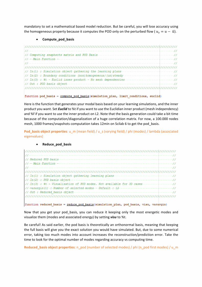
mandatorytosetamathematicalbasedmodelreduction.Butbecareful,youwillloseaccuracyusingthehomogeneouspropertybecauseitcomputesthePODonlyontheperturbedflow(𝑢" = 𝑢 −𝑢).

• Compute_pod_basis

Hereisthefunctionthatgeneratesyourmodalbasisbasedonyourlearningsimulations,andtheinnerproductyouwant.SetEuclidto%tifyouwanttousetheEuclidianinnerproduct(meshindependency)and%fifyouwanttousetheinnerproductonL2.Notethatthebasisgenerationcouldtakeabittimebecauseofthecomputation/diagonalizationofahugecorrelationmatrix.Fornow,a100.000nodesmesh,1000frames/snapshotscomputationtakes12minonScilab6togetthepod_basis.

Pod_basisobjectproperties:u_m(meanfield)/u_s(varyingfield)/phi(modes)/lambda(associatedeigenvalues)

• Reduce_pod_basis

Now that you get your pod_basis, you can reduce it keeping only themost energeticmodes andvisualizethem(modesandassociatedenergy)bysettingvisuto%t.

Becareful!Assaidearlier,thepodbasisistheoreticallyanorthonormalbasis,meaningthatkeepingthefullbasiswillgiveyoutheexactsolutionyouwouldhavesimulated.But,duetosomenumericalerror, taking toomuchmodes intoaccount increases the reconstruction/predictionerror.Take thetimetolookfortheoptimalnumberofmodesregardingaccuracyvscomputingtime.

Reduced_basisobjectproperties:n_pod(numberofselectedmodes)/phi(n_podfirstmodes)/u_m

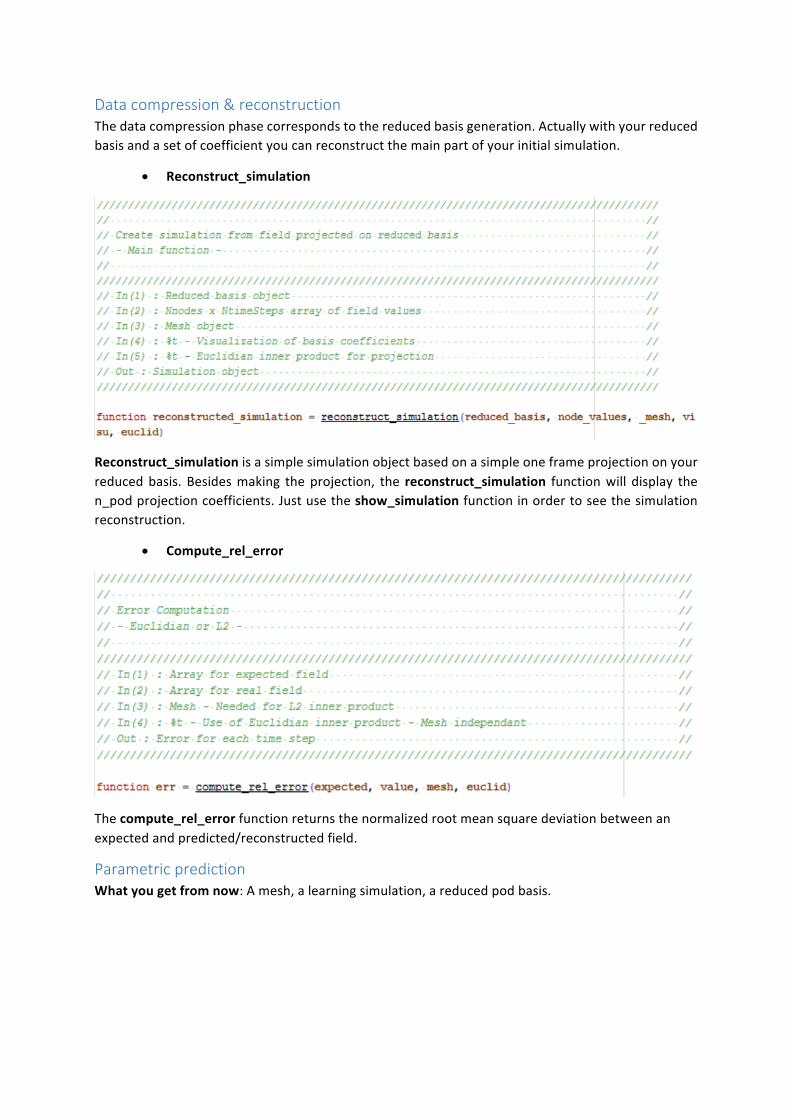
Datacompression&reconstructionThedatacompressionphasecorrespondstothereducedbasisgeneration.Actuallywithyourreducedbasisandasetofcoefficientyoucanreconstructthemainpartofyourinitialsimulation.

• Reconstruct_simulation

Reconstruct_simulationisasimplesimulationobjectbasedonasimpleoneframeprojectiononyourreducedbasis. Besidesmaking theprojection, the reconstruct_simulation functionwill display then_podprojectioncoefficients.Justusetheshow_simulationfunctioninordertoseethesimulationreconstruction.

• Compute_rel_error

Thecompute_rel_errorfunctionreturnsthenormalizedrootmeansquaredeviationbetweenanexpectedandpredicted/reconstructedfield.

ParametricpredictionWhatyougetfromnow:Amesh,alearningsimulation,areducedpodbasis.

1) Steadyparametricinterpolation

This function will first compute the projection coefficients on the reduced basis of your learningsimulationsandwillinterpolatethecoefficientsthenewparameterwithRadialBasisFunction.Todoso,youjustneedtosetyourentireDOEcomposedofyourparametersvaluesforeachsimulationcase,one parameter per column. Two different kernels are available: Gaussian andMultiquadric. If thesystemisill-conditioned,youcanaddrelaxationpolynomialswithorthogonalitycondition.Notethatthe choice of the interpolationmethoddepends on the physical field to predict. It is an empiricalprocess.

2) Unsteadymono-parametricinterpolationUnsteadysimulationsaremorecomplextopredictbecausewecan’tmakeasimpleinterpolationonthecoefficients,consideringthatthosearetime-andparameter-dependent.SoyouwillhavetomakeasecondPODonthereducedbasisyougot,usingn2_podfunction.Butfirst,makesurethatallyourunsteadysimulationshavethesamenumbersnapshots(=timesteps).

• N2_pod

Givingthenumberof learningparameters,thefirstreduced_basisandthe learningsimulation,thisfunctionreturnsanewPODbasisandtheassociatedcoefficients.Thosecoefficientsareusedfortheinterpolationinthefollowingfunction:

• One_parameter_interpolation

JustasRBF_interpolation,thisfunctionwillreturntheinterpolatedcoefficientsforthenewvalueofparameter,given theDOE (DOE–have tobe linevector), thenumberofmodesn_pod in the firstreducedbasisandthecoefficientsgivenbythen2_podfunction.

3) PredictionWhatyougetfromnow:Amesh,learningsimulation,reducedpodbasisandinterpolatedcoefficientsNewPInterp.

• Predict_simulation

The predict_simulation function creates the predicted simulation associated to the interpolatedcoefficients.Ifyouhaveusedthen2_podfunctiontogetinterpolatedcoefficientsforyourunsteadysimulation, setn2 inputargument to%tandadd thesecondPODbasispodi generatedbyn2_podfunction.

VisualizationSome visualization functions are already used in themain functions, but it may be interesting toleveragesomeofthemwithoutgeneratingafullPODbasis,again.

• Plot_basis_coefficients

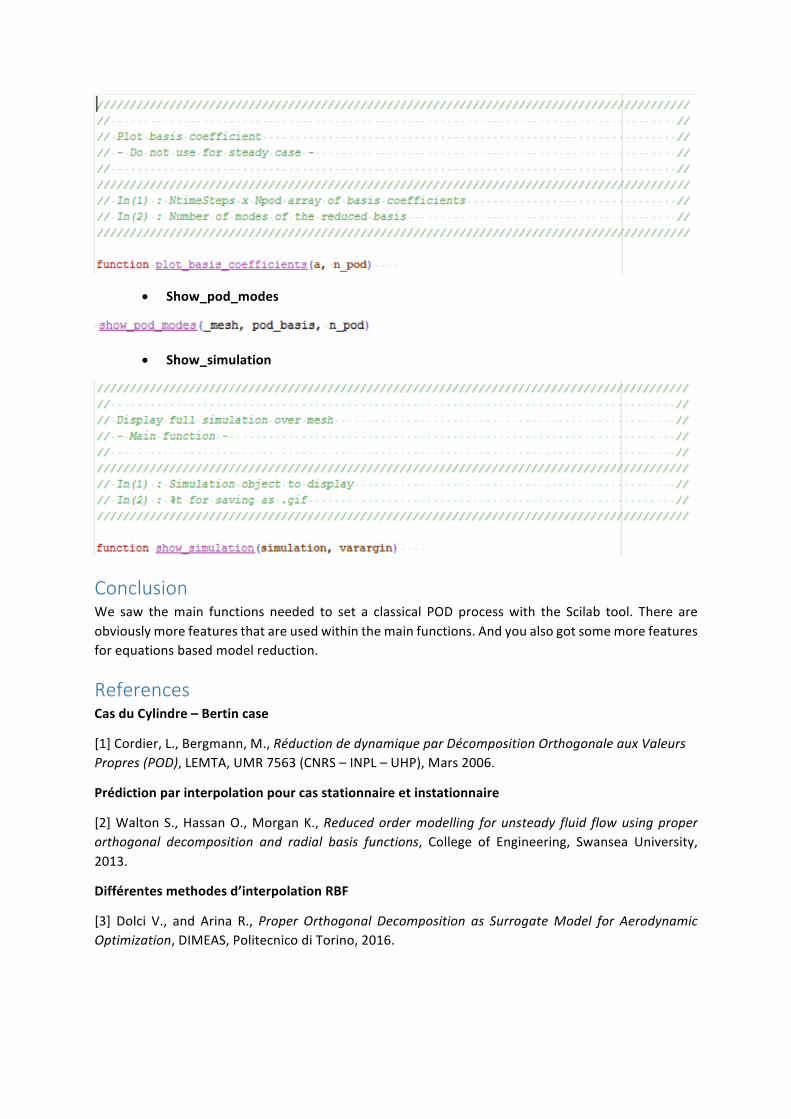
• Show_pod_modes

• Show_simulation

ConclusionWe saw themain functions needed to set a classical POD processwith the Scilab tool. There areobviouslymorefeaturesthatareusedwithinthemainfunctions.Andyoualsogotsomemorefeaturesforequationsbasedmodelreduction.

ReferencesCasduCylindre–Bertincase

[1]Cordier,L.,Bergmann,M.,RéductiondedynamiqueparDécompositionOrthogonaleauxValeursPropres(POD),LEMTA,UMR7563(CNRS–INPL–UHP),Mars2006.

Prédictionparinterpolationpourcasstationnaireetinstationnaire

[2]WaltonS.,HassanO.,MorganK.,Reducedordermodelling forunsteady fluid flowusingproperorthogonal decomposition and radial basis functions, College of Engineering, Swansea University,2013.

Différentesmethodesd’interpolationRBF

[3] Dolci V., and Arina R.,Proper Orthogonal Decomposition as SurrogateModel for AerodynamicOptimization,DIMEAS,PolitecnicodiTorino,2016.