scientific visualization of n-dimensional attainable …tpeterka/papers/peterka-thesis03.pdf ·...
TRANSCRIPT

SCIENTIFIC VISUALIZATION OF N-DIMENSIONAL ATTAINABLE REGIONS
BY
THOMAS PETERKA B.S., University of Illinois at Chicago, 1987
THESIS
Submitted as partial fulfillment of the requirements for the degree of Master of Science in Computer Science
in the Graduate College of the University of Illinois at Chicago, 2003
Chicago, Illinois

This thesis is dedicated to Melinda, Chris, and Amanda, whose unwavering support and
encouragement helped make a distant dream become a reality.
iii

ACKNOWLEDGEMENTS I would like to thank the following people individually for their contributions to this work. Some are
thesis committee members, others collaborators in one form or another. All were instrumental to the
success of this thesis and I am deeply indebted to them.
• Andrew Johnson of the Electronic Visualization Laboratory (EVL), University of Illinois at Chicago
(UIC) for helpful feedback and review of the thesis
• Jason Leigh, EVL, UIC for continued support and helpful input
• John Bell, lecturer, UIC. Dr. Bell tirelessly reviewed weekly progress, arranged collaborations, and
was instrumental in the success of this work from start to finish. His enthusiasm, involvement, and
high expectations helped this thesis become a truly meaningful endeavor.
• Peter Nelson, CS department head, UIC, for ongoing overseeing of the work
• Tumisang Seodigeng, researcher, Center of Process and Material Synthesis, School of Process
and Materials Engineering, University of Witwatersrand, Johannesburg, South Africa. Mr.
Seodigeng was most helpful with the second sample problem, and was our collaborator in the field
doing actual AR research. I am thankful not only for his data set, but for the invaluable feedback
as well.
• David Glasser, and Brendon Hausberger of the University of Witwatersrand, Johannesburg, South
Africa also for their collaboration on the second sample problem.
• Ken Clarkson, researcher, Bell Labs, Murray Hill, New Jersey. Mr. Clarkson generously provided
an open-source application for computing convex hulls in general numbers of dimensions. His
code was very reliable, and it played a valuable role in the visualization of the second sample
problem.
TP
iv
TABLE OF CONTENTS CHAPTER PAGE
1. INTRODUCTION ....................................................................................................... 1 2. BACKGROUND ......................................................................................................... 5 2.1 Computer Graphics and Virtual Reality......................................................... 5 2.1.1 CAVE ............................................................................................................ 6 2.1.2 Tiled Displays ............................................................................................... 7 2.1.3 Auto-Stereoscopic Displays ......................................................................... 9 2.1.4 Desktop Displays ....................................................................................... 10 2.2 User Interface Design ................................................................................ 11 2.2.1 Transparency .............................................................................................. 11 2.2.2 Direct Manipulation .................................................................................... 12 2.2.3 Building Tools.............................................................................................. 12 2.2.4 Color ........................................................................................................... 15 2.2.5 Testing and Evaluation ............................................................................... 16 2.3 Scientific Visualization ................................................................................ 18 2.3.1 General Principles ...................................................................................... 18 2.3.2 Multivariate Visualization ............................................................................ 20 2.3.3 Dimensional Attributes ............................................................................... 20 2.3.4 Animation ................................................................................................... 21 2.3.5 Dimension Reduction ................................................................................. 22 2.3.6 Coordinates and Coordinate Systems ....................................................... 23 2.3.7 Dimensionality ............................................................................................ 25 2.3.8 Convex Hulls .............................................................................................. 27 2.4 Attainable Regions ...................................................................................... 29 2.4.1 Attainable Region Theory ........................................................................... 31 2.4.2 Terminology and Definitions ....................................................................... 32 2.4.3 Fundamental Reactor Types and Operations ............................................ 32 2.4.4 Properties of the Attainable Region ........................................................... 37 2.4.5 Features of the Attainable Region ............................................................. 38 2.4.6 Current Attainable Region Visualizations.................................................... 39
3. APPLICATION DEVELOPMENT ............................................................................ 42 3.1 Introduction ................................................................................................. 42 3.2 Platforms .................................................................................................... 44 3.3 N-Dimensional Architecture ....................................................................... 47 3.4 Data File Format ........................................................................................ 49 3.5 Tetrahedral Coordinates ............................................................................ 51 3.6 Dimension Reduction .................................................................................. 52 3.6.1 User Interface.............................................................................................. 52 3.6.2 Relationship to Attainable Region Properties ............................................ 54 3.7 Convex Hulls Revisited ............................................................................... 57 3.7.1 View-Based 3-d Convex Hull ..................................................................... 57 3.7.2 General n-d Full Convex Hull ..................................................................... 58 3.8 Surface Rendering ..................................................................................... 60 3.9 Lighting ....................................................................................................... 64 3.10 Data Probing .............................................................................................. 66 3.10.1 Probing Points and Curves ........................................................................ 66 3.10.2 Probing Surfaces ........................................................................................ 67 3.10.3 Labeling ...................................................................................................... 69 3.11 Grid Scale Values ....................................................................................... 72
v

TABLE OF CONTENTS (continued)
CHAPTER PAGE 4. SAMPLE PROBLEM 1............................................................................................. 74 4.1 Equations and Rate Laws .......................................................................... 74 4.2 Results ....................................................................................................... 75 5. SAMPLE PROBLEM 2 ............................................................................................ 78 6. CONCLUSION ........................................................................................................ 83 6.1 Summary .................................................................................................... 83 6.2 Accomplishments ....................................................................................... 84 6.3 Future Work ................................................................................................ 85 CITED LITERATURE .............................................................................................. 87 APPENDICES ......................................................................................................... 90 Appendix A .............................................................................................................. 90 Appendix B .............................................................................................................. 95 Appendix C ........................................................................................................... 101 Appendix D ........................................................................................................... 104 VITA .................................................................................................................. 109
vi

LIST OF TABLES TABLE PAGE
I. SURVEY OF AR LITERATURE ................................................................................................. 41 II. MAJOR CONTRIBUTIONS AND OTHER ACCOMPLISHMENTS ............................................ 85
vii
LIST OF FIGURES FIGURE PAGE
1. Sample process flowchart ............................................................................................................. 2 2. CAVE architecture........................................................................................................................ 7 3. Tiled LCD display .......................................................................................................................... 8 4. Tiled projector display ................................................................................................................... 8 5. Auto-stereo 4-panel display ........................................................................................................ 10 6. Basic window elements ............................................................................................................... 13 7. Examples of dialog boxes ........................................................................................................... 14 8. Help system ................................................................................................................................ 14 9. Use of color as an identification tool ........................................................................................... 16 10. Daily weather map ...................................................................................................................... 20 11. Air quality visualization ................................................................................................................ 21 12. Ternary diagram.......................................................................................................................... 24 13. Tetrahedral coordinates .............................................................................................................. 25 14. Non-ideal reactor represented using ideal models...................................................................... 29 15. Modern chemical plant ................................................................................................................ 30 16. Plug flow reactor ......................................................................................................................... 33 17. Differential side-stream reactor ................................................................................................... 34 18. Continuous stirred tank reactor ................................................................................................... 35 19. Mixing.......................................................................................................................................... 36 20. Curved and ruled surfaces .......................................................................................................... 38 21. Data structure for storing n-d points ............................................................................................ 47 22. MVC model ................................................................................................................................. 48 23. Program structure ....................................................................................................................... 48 24. Collaborative approach to visualization....................................................................................... 49 25. 4-d tetrahedral view..................................................................................................................... 51 26. Coordinate system properties ..................................................................................................... 53 27. Triangulating between two curves............................................................................................... 60 28. Regular and skewed triangles..................................................................................................... 61 29. Good and bad triangulations ....................................................................................................... 63 30. Interpolating probed data ............................................................................................................ 69 31. Use of labels ............................................................................................................................... 71 32. Scale values dialog box .............................................................................................................. 72 33. Sample problem 1 results ........................................................................................................... 75 34. Sample problem 1 tetrahedral view............................................................................................. 76 35. Tetrahedral view of sample problem 2 ........................................................................................ 79 36. Tetrahedral view with visible convex hull .................................................................................... 80 37. Tetrahedral view with trace amounts of component E ................................................................ 81 38. Orthogonal view of B,C,D............................................................................................................ 81
viii

LIST OF ABBREVIATIONS
2-d, 3-d, 4-d, n-d 2-dimensional, 3-dimensional, 4-dimensional, n-dimensional
AR attainable region
CAVE CAVE Automatic Virtual Environment
CG computer graphics
CRT cathode ray tube
CSTR continuous stirred tank reactor
DSR differential side stream reactor
EVL Electronic Visualization Laboratory
GUI graphical user interface
LCD liquid crystal display
MFC Microsoft Foundation Classes
MVC model view controller
PC personal computer
PFR plug flow reactor
RAM random access memory
UIC University of Illinois at Chicago
VR virtual reality
ix
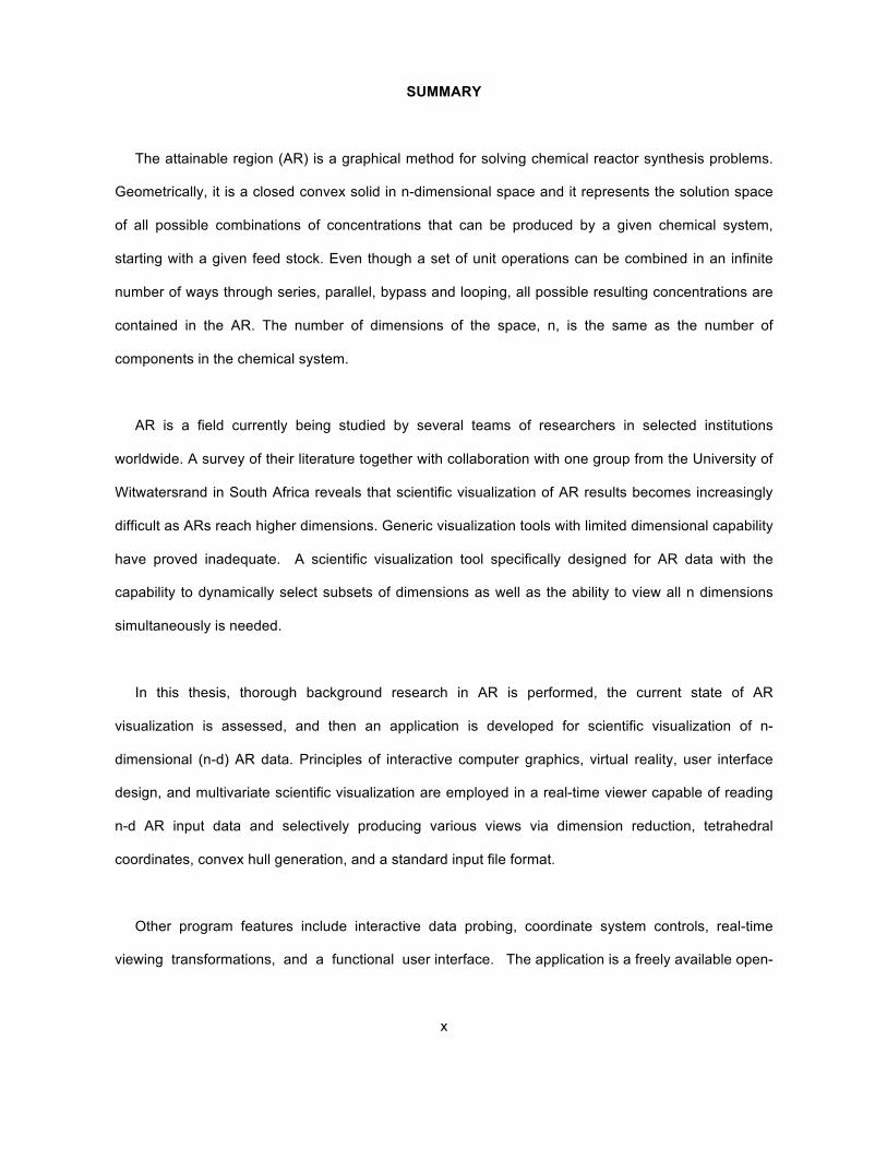
SUMMARY
The attainable region (AR) is a graphical method for solving chemical reactor synthesis problems.
Geometrically, it is a closed convex solid in n-dimensional space and it represents the solution space
of all possible combinations of concentrations that can be produced by a given chemical system,
starting with a given feed stock. Even though a set of unit operations can be combined in an infinite
number of ways through series, parallel, bypass and looping, all possible resulting concentrations are
contained in the AR. The number of dimensions of the space, n, is the same as the number of
components in the chemical system.
AR is a field currently being studied by several teams of researchers in selected institutions
worldwide. A survey of their literature together with collaboration with one group from the University of
Witwatersrand in South Africa reveals that scientific visualization of AR results becomes increasingly
difficult as ARs reach higher dimensions. Generic visualization tools with limited dimensional capability
have proved inadequate. A scientific visualization tool specifically designed for AR data with the
capability to dynamically select subsets of dimensions as well as the ability to view all n dimensions
simultaneously is needed.
In this thesis, thorough background research in AR is performed, the current state of AR
visualization is assessed, and then an application is developed for scientific visualization of n-
dimensional (n-d) AR data. Principles of interactive computer graphics, virtual reality, user interface
design, and multivariate scientific visualization are employed in a real-time viewer capable of reading
n-d AR input data and selectively producing various views via dimension reduction, tetrahedral
coordinates, convex hull generation, and a standard input file format.
Other program features include interactive data probing, coordinate system controls, real-time
viewing transformations, and a functional user interface. The application is a freely available open-
x

SUMMARY (continued)
source program that runs on most personal computers (PCs) under most versions of the Windows
operating systems. Virtual reality devices such as the CAVE, tiled display, and auto-stereoscopic
display have been examined as part of the background study, and feasibility for future migration of the
application to these devices is assessed.
Two sample problems are documented, the first theoretical and the second an actual data set from
current AR research. Collaboration with researchers has helped the application to evolve, and the
program and results have been shared to help guide researchers in further studies. Preliminary
feedback from collaborators has been positive. The overall contribution of this thesis is to provide an
interactive visualization tool for n-d ARs, which is needed to help AR research move to higher
dimensions.
xi
1
1. INTRODUCTION
Chemical engineering, like other engineering disciplines, often relies on graphical methods for
solving complex problems. This works well for “textbook” problems, but unfortunately graphical
methods are difficult to apply to many "real" problems because they are often much more complex.
The increased complexity is due to increased number of variables, ie. larger dimensional space. For
example, sample graphical problems are usually two-dimensional, while real problems may contain 5
or 10 variables. However, graphical solutions offer advantages over other numerical methods
because of the visual perception of the human mind, so graphical solutions for multivariate problems
are desirable. While it is difficult to visualize high dimensional data, a good visualization will reward the
engineer with extremely comprehensible results.
One such graphical method in chemical engineering is called "attainable regions", or AR. This is a
geometric representation of the solution space of all possible combinations of selected unit operations
for a system of chemical reactions, starting from a given feed point. The chemical engineer desires to
find an optimal flowchart combination of reactors and mixers to optimize some objective function, such
as production of a desired component, and the first step in this optimization process is to determine
what compositions are feasible, or attainable. The attainable region is a convex closed solid in n-
dimensional space, where n is the number of components in the chemical system.
The following example will serve to introduce ARs, especially to those readers with backgrounds
other than in the field of chemical engineering. Suppose that an engineer is charged with the task of
designing a new chemical plant consisting of a set of chemical reactors and mixers to operate on
some given chemical system such as below. (van de Vusse, 1964)
A1 ! A2
A2 ! A4
2A1 ! A3

2
Usually the goal is to maximize some objective function, for example maximizing production of A4
while minimizing the number of reactors used. The engineer also has a set of fundamental operations
to choose from. In this thesis, 4 ideal operations are considered: 3 types of reactors and bulk mixing.
Each of these can be described by an ideal model governed by a differential or algebraic equation.
The difficulty lies in the fact that the unit operations can be combined in an infinite number of ways
using series, parallel, bypass, looping, etc. For example, Figure 1 below shows a small flowchart of
several reactors connected together.
Figure 1. Sample process flowchart
Since the number of combinations of processes is infinite, the engineer has two choices. Either he
may reduce the number of possibilities by applying heuristics, rules of thumb, or historical experience,
or apply a more systematic scientific method. Obviously the latter is preferred, and ARs provide this
method. The AR is easy to visualize when the number of dimensions is small, say two or three, but
difficult to visualize when higher dimensions are used. Not surprisingly, it is just these high-
dimensional (high-d) ARs that occur in real-life chemical engineering situations, as opposed to low-d
“textbook” examples.

3
A survey of AR literature reveals that the current state of AR visualization follows two patterns.
Either the number of variables visualized is reduced (for example from 5 down to 2 or 3), or high-d
results produced by numerical methods may not be visualized at all. (See Section 2.4.6 for more
details.) The whole basis for the AR method first invented by Horn (Horn, 1964) is to see the space of
all possibilities, which then can lead to rational optimization paths. A useful n-d visualization tool
specifically designed for AR data can eliminate the necessity to discard variables, and provide a
visualization of data where there was none before.
A collaboration was formed with a key research group currently pursuing the study of high-d ARs.
A working partnership with the University of Witwatersrand, in Johannesburg, South Africa was begun
and a need was discovered for high-d visualization of AR results. A scientific visualization program
was developed as part of this thesis work which can interactively produce views based on dimension
reduction, tetrahedral coordinates, and convex hull generation. Other features include data probing,
real-time viewing transformations, and a functional user interface including online help. Through the
use of a standard file format (also developed as part of this thesis), researchers are able to focus on
what they do best, simulating and producing data sets, freeing them from developing visualization
methods.
Two sample problems were tested, 4-dimensional and 5-dimensional, and the application is
designed to accept even larger problem spaces. Concepts from several different disciplines are
employed, from chemical engineering, scientific visualization, and computer science. Chemical
engineering provides the basis for the AR method of modeling reactor synthesis, while concepts from
the study of scientific visualization to graphically represent high-d data are utilized to maximize
comprehension. Finally, several topics in computer science are explored to develop the computer
application that serves as the visualization tool, such as 3-d computer graphics, virtual reality, and
user interface design.
4
The following is a list of specific enhancements or additions that this thesis contributes to the
current state of AR visualization. The following chapters provide background and detail as to how this
was accomplished.
• Providing an interactive AR-specific visualization tool capable of maintaining all dimensions of a
problem space and selectively displaying a subset of dimensions under various settings as well
as displaying all dimensions simultaneously if desired
• Applying the tetrahedral coordinate system to AR visualization, which does not appear in any AR
literature as yet but is a useful display paradigm for chemical engineers and researchers
• Using n-d and 3-d convex hulls to view disorganized data sets and to filter extraneous data from
large data sets prior to viewing, allowing these data to be viewed as well
• Developing a standard file format for the transmission of data sets between simulation programs
and the visualization, enhancing communication of results between research organizations
5
2. BACKGROUND
A synthesis of concepts from the studies of AR, scientific visualization, and computer science form
the background material for the thesis. Computer science topics include a discussion of computer
graphics, virtual reality, and user interface design. Scientific visualization, specifically multivariate
visualization is explored in order to display higher numbers of dimensions within a limited dimensional
space. ARs are researched in order to understand AR theory, properties and features of the AR, and
the current state of visualization in this domain.
2.1 Computer Graphics and Virtual Reality
3d computer graphics (CG) is the rendering of objects in three-dimensional world-space onto a two-
dimensional computer display device; typical applications are computer aided design, user interfaces,
games, and artistic expression. Virtual reality (VR) is an extension of 3d computer graphics through
specialized software and hardware for the purpose of creating a sense of immersion in the computer
application. The list of applications suitable for VR is similar those for CG. Sherman and Craig define
VR as: “a medium composed of interactive computer simulations that sense the participant’s position
and actions or augment the feedback to one or more senses, giving the feeling of being mentally
immersed or present in the simulation (a virtual world).” (Sherman and Craig, 2003)
This is a specific textbook definition that also enumerates some key ingredients of VR, namely
position tracking, sensory feedback, and immersion. CG and VR are considered together in this thesis
as they relate to scientific visualization with the aim of maximizing data comprehension. What follows
is a very brief introduction to some common CG/VR display devices and systems as they relate to the
AR visualization. Some devices such as the CAVE are where the work began, others such as laptops
and PCs are the current platform, and still others such as tiled displays and auto-stereo displays are
the future intended targets for the AR work.
6
2.1.1 CAVE
The CAVE, or CAVE Automatic Virtual Environment, was invented at the Electronic Visualization
Laboratory (EVL) at the University of Illinois at Chicago (UIC) in 1992. (Cruz-Neira et al., 1992) It is a
10-foot x 10-foot x 10-foot cube in which several participants can stand simultaneously. Viewers are
surrounded by three walls of rear-projection screens, and together with the floor, this constitutes four
surfaces onto which images are seamlessly projected through the use of high quality projectors and
mirrors. Images are projected in field-sequential stereo, meaning that images alternate between left
and right eyes through the use of synchronized LCD shutter glasses to create a stunning 3d effect.
One viewer’s position is tracked through an ultrasonic tracking system, and the viewpoint is updated in
real-time to maintain first-person perspective. Finally, a high quality sound system is included.
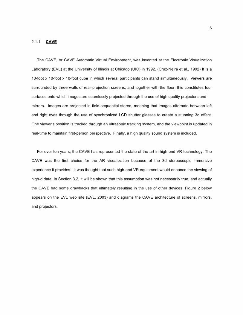
For over ten years, the CAVE has represented the state-of-the-art in high-end VR technology. The
CAVE was the first choice for the AR visualization because of the 3d stereoscopic immersive
experience it provides. It was thought that such high-end VR equipment would enhance the viewing of
high-d data. In Section 3.2, it will be shown that this assumption was not necessarily true, and actually
the CAVE had some drawbacks that ultimately resulting in the use of other devices. Figure 2 below
appears on the EVL web site (EVL, 2003) and diagrams the CAVE architecture of screens, mirrors,
and projectors.
7
Figure 2. CAVE architecture (image courtesy of EVL)
2.1.2 Tiled Displays
For years, VR technology was primarily either projection-based or head-based. Only recently has a
third display option emerged: tiled. A tiled display is a matrix of smaller individual displays, driven by a
cluster of PCs, and assembled to make a large-size, high resolution, high brightness, wide field of
view display. The individual components can be either liquid-crystal display panels (LCDs) or
projectors. EVL at UIC has been one of the innovators of the LCD tiled display, with their “Perspectile”
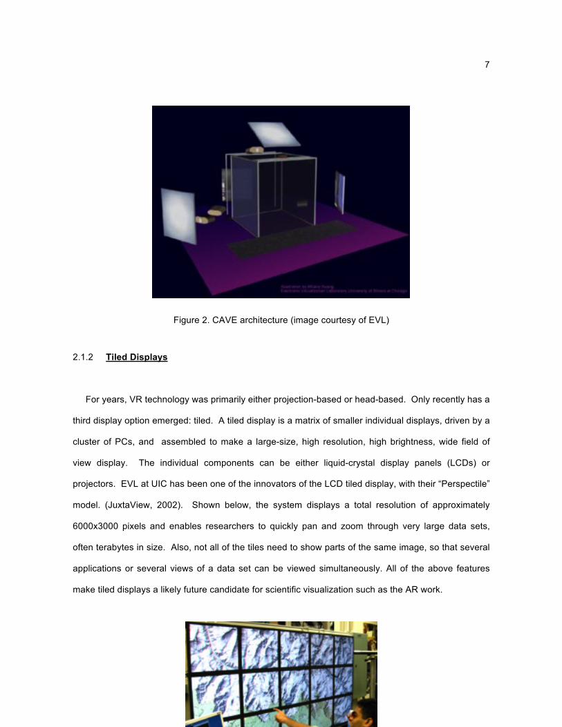
model. (JuxtaView, 2002). Shown below, the system displays a total resolution of approximately
6000x3000 pixels and enables researchers to quickly pan and zoom through very large data sets,
often terabytes in size. Also, not all of the tiles need to show parts of the same image, so that several
applications or several views of a data set can be viewed simultaneously. All of the above features
make tiled displays a likely future candidate for scientific visualization such as the AR work.
8
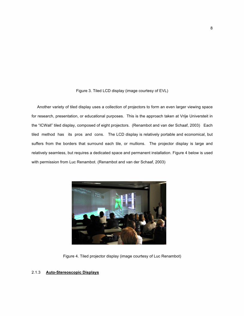
Figure 3. Tiled LCD display (image courtesy of EVL)
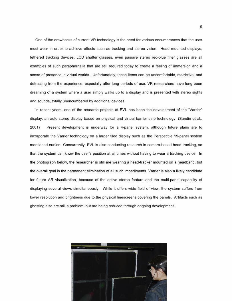
Another variety of tiled display uses a collection of projectors to form an even larger viewing space
for research, presentation, or educational purposes. This is the approach taken at Vrije Universteit in
the “ICWall” tiled display, composed of eight projectors. (Renambot and van der Schaaf, 2003) Each
tiled method has its pros and cons. The LCD display is relatively portable and economical, but
suffers from the borders that surround each tile, or mullions. The projector display is large and
relatively seamless, but requires a dedicated space and permanent installation. Figure 4 below is used
with permission from Luc Renambot. (Renambot and van der Schaaf, 2003)
Figure 4. Tiled projector display (image courtesy of Luc Renambot)
2.1.3 Auto-Stereoscopic Displays
9
One of the drawbacks of current VR technology is the need for various encumbrances that the user
must wear in order to achieve effects such as tracking and stereo vision. Head mounted displays,
tethered tracking devices, LCD shutter glasses, even passive stereo red-blue filter glasses are all
examples of such paraphernalia that are still required today to create a feeling of immersion and a
sense of presence in virtual worlds. Unfortunately, these items can be uncomfortable, restrictive, and
detracting from the experience, especially after long periods of use. VR researchers have long been
dreaming of a system where a user simply walks up to a display and is presented with stereo sights
and sounds, totally unencumbered by additional devices.
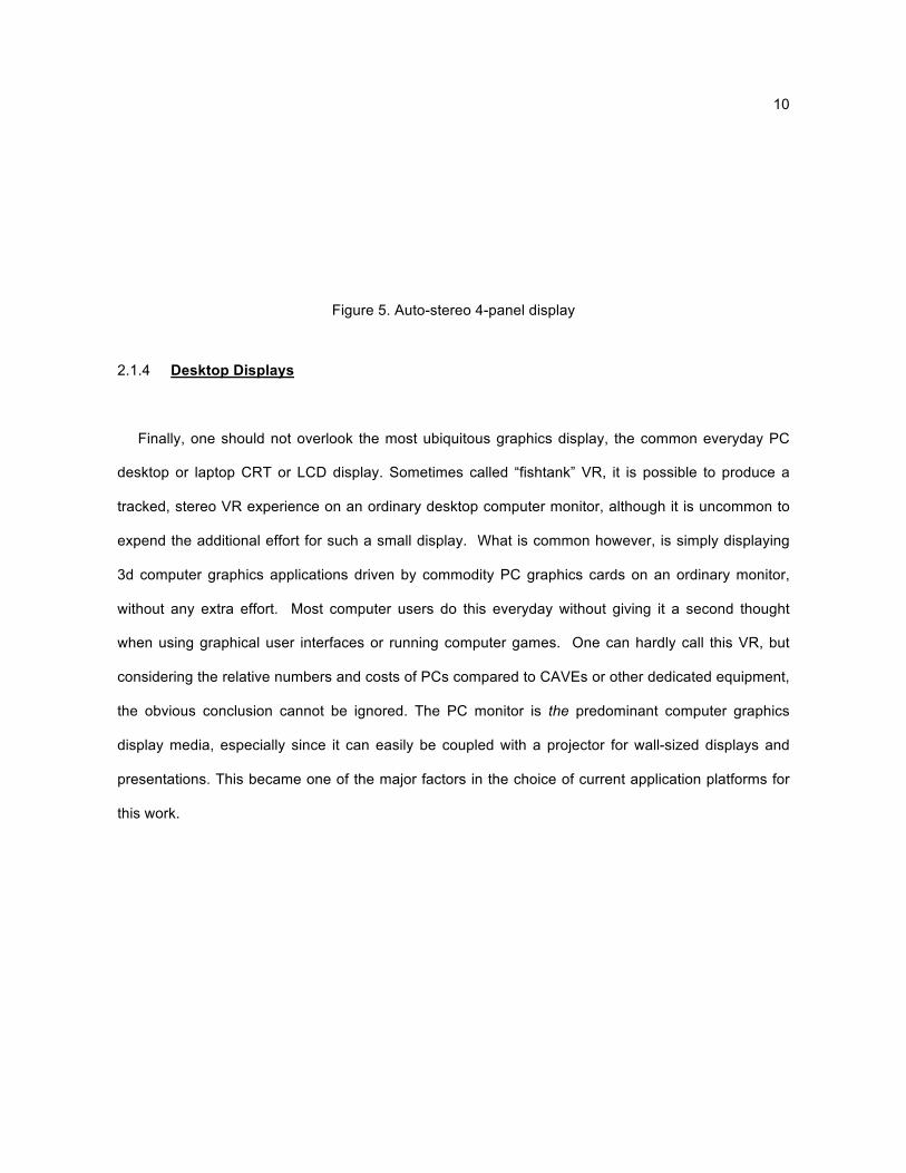
In recent years, one of the research projects at EVL has been the development of the “Varrier”
display, an auto-stereo display based on physical and virtual barrier strip technology. (Sandin et al.,
2001) Present development is underway for a 4-panel system, although future plans are to
incorporate the Varrier technology on a larger tiled display such as the Perspectile 15-panel system
mentioned earlier. Concurrently, EVL is also conducting research in camera-based head tracking, so
that the system can know the user’s position at all times without having to wear a tracking device. In
the photograph below, the researcher is still are wearing a head-tracker mounted on a headband, but
the overall goal is the permanent elimination of all such impediments. Varrier is also a likely candidate
for future AR visualization, because of the active stereo feature and the multi-panel capability of
displaying several views simultaneously. While it offers wide field of view, the system suffers from
lower resolution and brightness due to the physical linescreens covering the panels. Artifacts such as
ghosting also are still a problem, but are being reduced through ongoing development.
10
Figure 5. Auto-stereo 4-panel display
2.1.4 Desktop Displays
Finally, one should not overlook the most ubiquitous graphics display, the common everyday PC
desktop or laptop CRT or LCD display. Sometimes called “fishtank” VR, it is possible to produce a
tracked, stereo VR experience on an ordinary desktop computer monitor, although it is uncommon to
expend the additional effort for such a small display. What is common however, is simply displaying
3d computer graphics applications driven by commodity PC graphics cards on an ordinary monitor,
without any extra effort. Most computer users do this everyday without giving it a second thought
when using graphical user interfaces or running computer games. One can hardly call this VR, but
considering the relative numbers and costs of PCs compared to CAVEs or other dedicated equipment,
the obvious conclusion cannot be ignored. The PC monitor is the predominant computer graphics
display media, especially since it can easily be coupled with a projector for wall-sized displays and
presentations. This became one of the major factors in the choice of current application platforms for
this work.
11
2.2 User Interface Design
User interface design is the study of developing applications to be usable by other people than just
the author of the program. As Andrew Johnson writes, “Making a program work for you is pretty easy.
Making it work for another user is much harder.” (Johnson, 2002) User interfaces are not limited only
to computer applications either; they are all around us in everyday life as well, (Norman, 1988) but this
discussion will be limited to a brief summary of “user centered design” as it pertains to this
visualization. It is interesting to note that some of the goals of interface design are similar to those of
scientific visualization. In a broad sense, the visualization is an interface to the underlying data, much
the same way as widgets and controls are an interface to a computer application.
The following is a brief outline of some of the guiding principles of user centered interface design,
especially as they pertain to the application in question. This section is condensed from an entire
semester-long course, and the interested reader is encouraged to consult any number of user
interface texts, such as Schneiderman. (Schneiderman, 1998)
2.2.1 Transparency
The first and probably most important characteristic of a good user interface is transparency. In
other words, the best interfaces are the ones the user never sees. In a perfect world, the user
concentrates only on the task at hand, in this case the attainable region, and never thinks about which
menu item or dialog box is needed or where that option is documented in the online help. Such a
perfect application has yet to be developed, but every now and then some individual feature is
implemented well, and its use becomes transparent.
12
2.2.2 Direct Manipulation
A closely related concept is direct manipulation. The more directly an action can be done, the more
transparent it will become. In this context, the word “direct” means simple, concise, or most closely
affording the intended result. This is what makes the “drag-and-drop” metaphor so attractive in
windows desktop systems, for example dragging a file icon to the trash icon in order to delete it. A
distinguishing feature of direct manipulation is direct feedback, much like the way a car is driven. One
does not think, “I will now turn the steering wheel 35 degrees to the right.” Rather, the driver turns the
wheel slightly and the result is immediately sensed. Then the driver turns more, etc., performing a
rapid series of incremental motions and adjustments while the task is smoothly executed. When direct
manipulation occurs so easily that it requires little or no conscious thought, it again becomes
transparent.
Navigation within the AR visualization is designed with this in mind. Real-time panning, zooming,
and rotating are accomplished using the wand in the CAVE version and the mouse in the PC version.
In the CAVE, the user points the wand in the desired direction of travel and manipulates the joystick or
trackball to control the speed of the motion. In the PC version, dragging the mouse with the right
mouse button depressed along with shift and control keys accomplishes the same result. Both
methods are easy to learn, and become transparent quickly. Both offer direct manipulation and
feedback, with sensitive speed control.
2.2.3 Building Tools
Microsoft foundation classes (MFC) within the Visual C++ environment provide tools for
constructing standard window controls such as menus, dialog boxes, toolbar buttons, and icons in an
application. There are other similar tools and libraries such as Borland C++ Builder, FLTK for Linux,
but the choice of particular tool is not the point. The idea is that the use of building tools is necessary

13
in modern user interface development. It affords rapid prototyping and the resulting interface is
uniform across the application and similar to other applications the user is already accustomed to.
What follows are a few examples of how a building tool such as MFC helped standardize the AR
visualization.
Window controls, menus, toolbar, icons
Included are standard drag-able title bar, minimize, maximize, close buttons, and re-sizable
borders. A status bar appears at the bottom with several panes to display file name and useful
messages. The main menu is straightforward with only two levels of depth, and a toolbar appears
below the menu with several icons for the common menu operations. See Figure 6 below.
Figure 6. Basic window elements
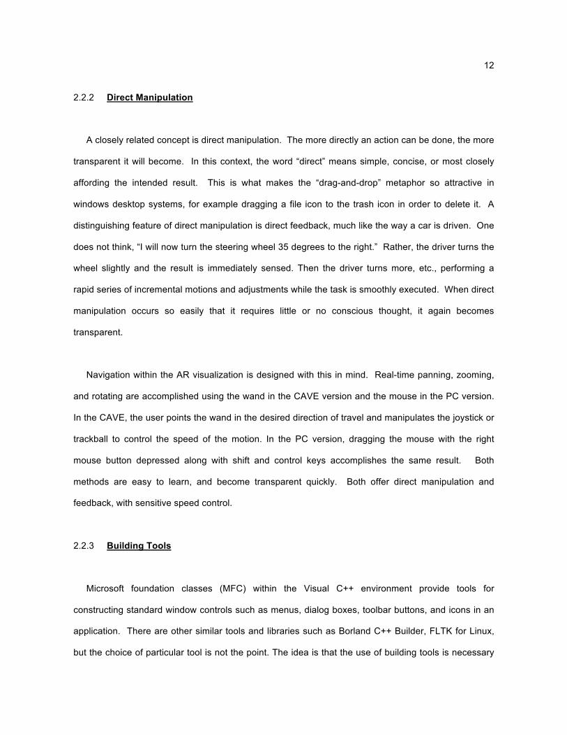
Dialog boxes
Dialog boxes are used to display information and to receive user input, as in the setting of various
options. The dialog shown below at left is the opening “splash” screen when the application starts up,
and is also used as the “help | about” screen. On the right is the scale values dialog box, an example
of a dialog used to set user options.
14
Figure 7. Examples of dialog boxes
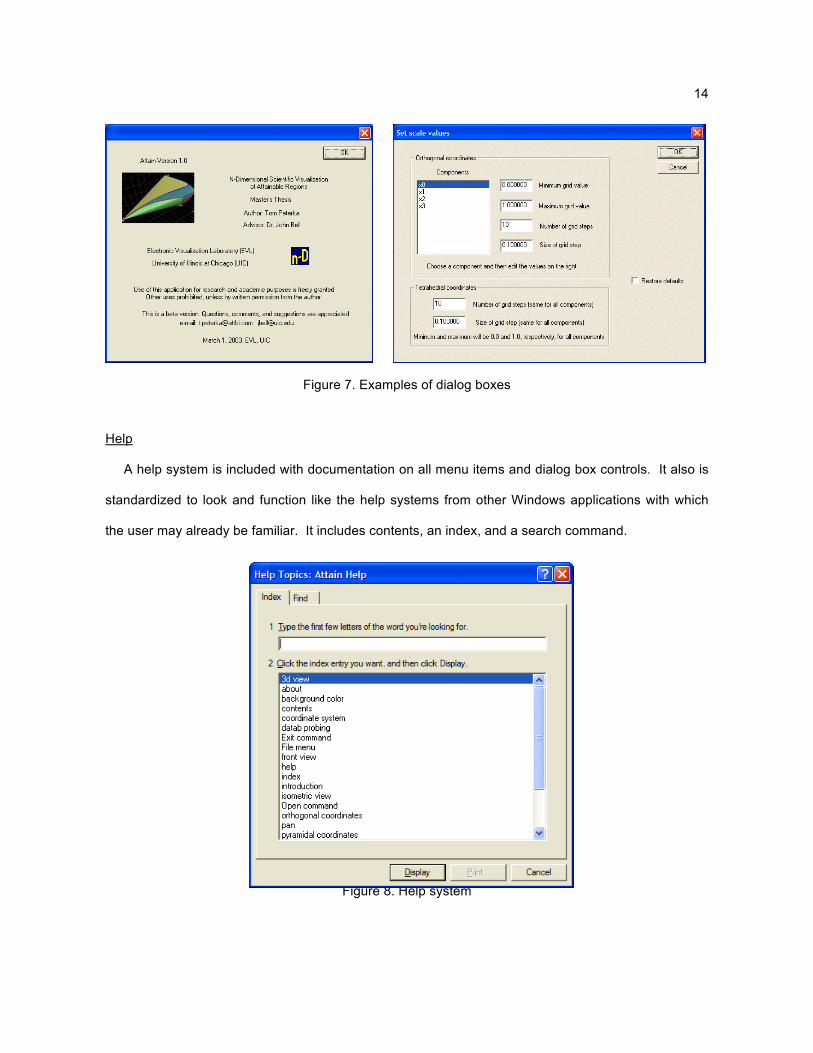
Help
A help system is included with documentation on all menu items and dialog box controls. It also is
standardized to look and function like the help systems from other Windows applications with which
the user may already be familiar. It includes contents, an index, and a search command.
Figure 8. Help system
15
2.2.4 Color
The effective use of color can be a tricky business. In a word processor or spreadsheet, color is
often used only as a highlighting mechanism, so it is easy to be conservative and use only 2 or 3
colors total. Other applications, especially scientific visualization, require a broad color spectrum
because color often conveys additional information such as an extra variable. (Nielson et al., 1997)
Unfortunately, color is also easy to misuse, resulting in color combinations that are difficult to see (eg.
red next to blue), unwanted meanings, or just plain unsightly displays. The opposite extreme is equally
bad: the over-use of color in order to produce an aesthetic display can mask the data’s true meaning,
the “pretty picture syndrome”. Finally, approximately 8 percent of men and .5 percent of women are
color-blind to some degree, making color even more difficult to use well.
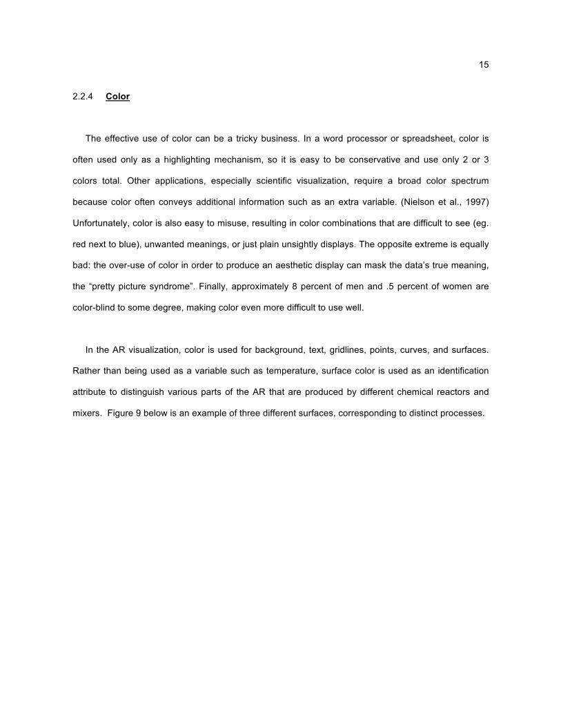
In the AR visualization, color is used for background, text, gridlines, points, curves, and surfaces.
Rather than being used as a variable such as temperature, surface color is used as an identification
attribute to distinguish various parts of the AR that are produced by different chemical reactors and
mixers. Figure 9 below is an example of three different surfaces, corresponding to distinct processes.
16
Figure 9. Use of color as an identification tool
Given the aforementioned difficulties in color selection, it becomes impossible to find color
combinations to satisfy everyone. So, the best policy is to let the user decide. Background and text
default to black and white respectively, but are selectable through color selection dialog boxes. Other
colors of geometric data objects are set through the input data file, documented in Appendix A. This
strategy is the best compromise to the color problem.
2.2.5 Testing and Evaluation
Testing and evaluation are major factors in user interface design, and the key is to test early and
often, rather than as an afterthought when the application is complete. The current state of the work
was reviewed on a weekly basis, so there were many opportunities to experiment and refine. Also,
our colleague, Tumi Seodigeng from the University of the Witwatersrand in Johannesbug, South
Africa, was supplied with several beta versions of the program, and provided input via e-mail.
Evaluation was largely informal, with comments and suggestions being implemented along the way.
Unfortunately, time did not allow for more formal techniques to be used on larger test groups of users.

17
However, a survey form to be used in the future as an evaluation instrument is included in Appendix
C.
18
2.3 Scientific Visualization
2.3.1 General Principles
Scientific visualization has its roots in the latter part of the eighteenth century with the graphs of
William Playfair, first published in 1786. (Tufte, 1983) It is not a new study, and goes by several names
including data visualization and data graphics. The goal of good visualization is to depict data visually,
graphically, or pictorially as opposed to only listing tables of numbers, in order to maximize data
comprehension. The old maxim, “A picture is worth a thousand words” applies here, as most people
recognize patterns and relationships graphically easier than numerically. Over the course of 200 years
or so, the discipline matured, and it became clear what comprises good quality, high-content data
graphics, at least in two dimensions on ink and paper.
Then, like so many areas, the field of scientific visualization was turned upside-down with the
advent of computer graphics, moreover with the availability of fast, cheap computer graphics
hardware. Computer-generated graphics began to be churned out at an amazing pace and with
incredible ease. Today, anyone who can enter numbers into a spreadsheet can produce printer tray-
fulls of charts and graphs in a matter of minutes. Of course, it is just as easy to produce bad, useless,
data-thin, and even nonsensical graphs at the same incredible pace. One does not have to look far to
find them either, usually a quick glance at any mass-produced news media will do.
Edward Tufte has written three excellent volumes on the study of data visualization, and he
devotes considerable effort characterizing the differences between good and bad graphics. (Tufte,
1983; Tufte, 1990; Tufte, 1997) What follows is only a brief list of some of his salient points.
19
According to Tufte, excellent graphics should:
1) show the data
2) encourage the viewer to focus on substance rather than design (transparency)
3) not distort the data (truthfulness)
4) present much information in a small space (high data density)
5) make large data sets coherent
6) encourage the drawing of comparisons and conclusions about the data
7) reveal several levels of detail, from broad to fine
8) display complex ideas with clarity, precision, and efficiency
9) display large numbers of variables (multivariate)
Tufte does a superb job elaborating on all of the above points and many others in his works and the
reader is encouraged to explore his volumes. The effort will be rewarded with a comprehensive and
interesting study of the history and theory of data visualization.
To repeat a previous concept, it is interesting to compare good interface design and good
visualization. Some points are identical: transparency, levels of detail, simple presentation of complex
ideas. Other aspects are specific to one topic of the other. Finally, in computer graphics scientific
visualizations, a widget or control or graphical element (eg. a button or dialog box) belongs both to the
user interface and to the visualization, so the topics become even more inter-twined. In this sense,
visualization is a broader concept than just the end-result graphic produced by the program. Rather,
visualization is the process of interacting with the data to producing desired and meaningful views of
the data, resulting ultimately in comprehension of the data.
20
2.3.2 Multivariate Visualization
The goal of this visualization research is to effectively display multivariate data (n-d) on a 2-d
device such as a computer screen, projection panel, or other VR or CG display medium. Keep in mind
that even 3-d computer graphics are still ultimately shown in 2-d, it is only our minds that are “fooled”
into thinking that we are seeing 3-d, since computer monitors and VR projection hardware still consist
of flat 2-d devices. So how do we “escape flatland”, as Edwin Abbot wrote over 100 years ago?
(Abbott, 1952; first published in 1884)
2.3.3 Dimensional Attributes
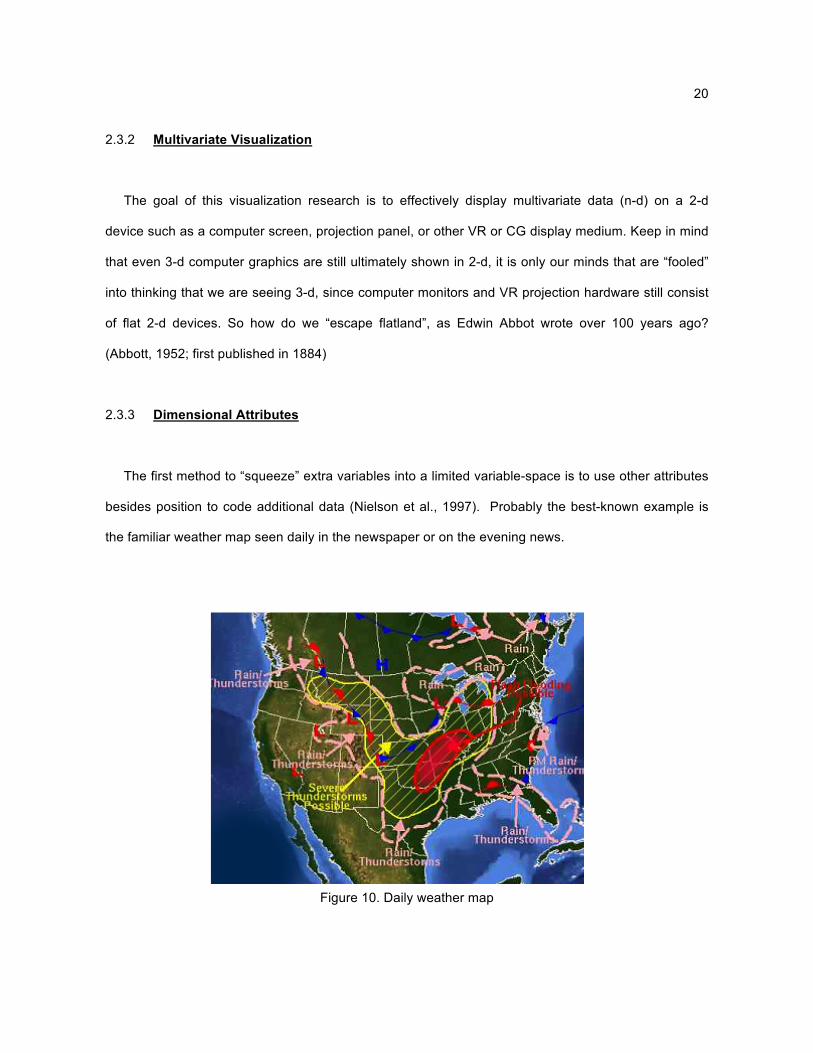
The first method to “squeeze” extra variables into a limited variable-space is to use other attributes
besides position to code additional data (Nielson et al., 1997). Probably the best-known example is
the familiar weather map seen daily in the newspaper or on the evening news.
Figure 10. Daily weather map

21
In Figure 10, 2-dimensional position is given by the (x,y) location of a point on the map. Since this is a
2-d graphic, no further positional variables can be displayed. So other attributes such as color,
shading, texture, annotations, etc. are used to extend the dimensional space beyond two dimensions.
Below is a slightly more complex example of the same idea.
Figure 11. Air quality visualization (courtesy Mike Rizzo and Tom Peterka)
Figure 11 is from an earlier project by the author and a partner from the U.S. Environmental
Protection Agency. The goal of the visualization was to search for a relationship between air
temperature and air quality, specifically ozone levels. This view compresses four dimensions onto a 2-
d computer screen. Three spatial dimensions are projected onto the 2-d display, and color is coded
for the fourth dimension. Specifically, (x,y) indicates the position along the earth in longitude and
latitude, z indicates ozone level, and color indicates temperature.
2.3.4 Animation
What Tufte calls “narratives of space and time,” (Tufte, 1990) is often called animation. When time
is one the variables, real-time computer graphics provides a direct and natural way to display it: to
22
show a “movie.” This is especially effective when the scene complexity and graphics hardware is such
that an acceptable frame rate (20-30 minimum frames per second) can be maintained so that smooth
motion results. To continue with the previous example, if ozone and temperature were displayed
across space and time (several hours, days, months, etc.), the display could be animated by
producing a time-series of individual snapshots as shown above, and played back along with a clock
display or time counter. The result would be compressing 5 dimensions down to 2.
2.3.5 Dimension Reduction
Multivariate display options are limited when there are multiple dimensions that cannot be codified
intuitively using animation, color, texture, or other display attributes. This is the nature of the problem
in the AR work. All dimensions in the problem space are spatial, and moreover the user will be
evaluating the AR based on geometric characteristics. Of particular importance is that an AR must be
convex, and the user will be looking for convexity in any of the produced views. Therefore, coding
spatial dimensions with color or other attributes is not useful. This leaves only one option: to view a
subset of dimensions at a time. Tufte calls this strategy “multiples”; (Tufte, 1997) the term used here
is dimension reduction, whereby the number of dimensions is reduced to three or four at any one time.
In dimension reduction, two strategies can reduce the dimensions of a space. One may either
project the data to the lower dimensional system, or create a cross-section through the data. A simple
example reducing three dimensions down to two will make this clear. Suppose a sphere in 3d is to be
projected to 2d. The result is essentially a top-down view of the sphere, a circle whose diameter is the
same as the diameter of the sphere. On the other hand, in a cross-section, a sectioning plane is
specified and the resulting view will be the intersection of the original model with the section plane.
Continuing with the sphere example, the result will be a circle again, but probably a smaller diameter
than the sphere depending on the position and orientation of the section plane. In the general n-d
case, the original model is n-dimensional and a subset of dimensions is viewed via projection or
23
section. The section plane becomes a hyper-plane, or a higher dimensional plane formed by fixing
various coordinates at specific values. Higher dimensional entities are discussed in more detail in
Section 2.3.7.
2.3.6 Coordinates and Coordinate Systems
Without coordinates, a visualization is nothing but a pretty picture. It is the assigning of coordinate
values that quantifies a data set and permits its visualization. There are many types of coordinate
systems, not just the familiar Cartesian. For example, logarithmic, polar, spherical, parabolic, etc. are
all possibilities. The choice of a coordinate system is not arbitrary; there are two reasons for choosing
one over another for a given application. First, a system may naturally lend itself to the data and
simplify the problem. For example, certain problems are much easier to solve in polar or spherical
coordinates because the equations are simpler and the number of coordinates fewer.
The other factor is comprehension. The real goal of scientific visualization is to tell a story about
the data (Tufte, 97). Data for its own sake is worthless; the value is in conclusions that are drawn,
inferences made, comparisons generated. The choice of coordinate system is critical because
patterns can become clear in one system that were obscured in another, just as a constant growth rate
pattern may not be obvious on a linear scale but takes the familiar straight-line form on a logarithmic
scale.
Besides the type of coordinate system, scale ranges and resolutions are also critical. If the goal is
to tell a story about the data, the interesting parts may be missed by looking in the wrong places, not
looking closely enough, or looking too closely and “missing the forest for the trees”. This is all a matter
of setting appropriate scale ranges and scale steps.
24
In the AR application, two types of coordinate systems are utilized to plot chemical concentrations
and mole fractions. Cartesian coordinates are used in 3-d concentration space, where concentration is
measured in amount per unit volume, such as moles per liter. The second coordinate system is called
“tetrahedral coordinates”. Here the plotted values are mole fraction rather than concentration, and
there are no units because the measurement is a fraction of the desired concentration to the whole.
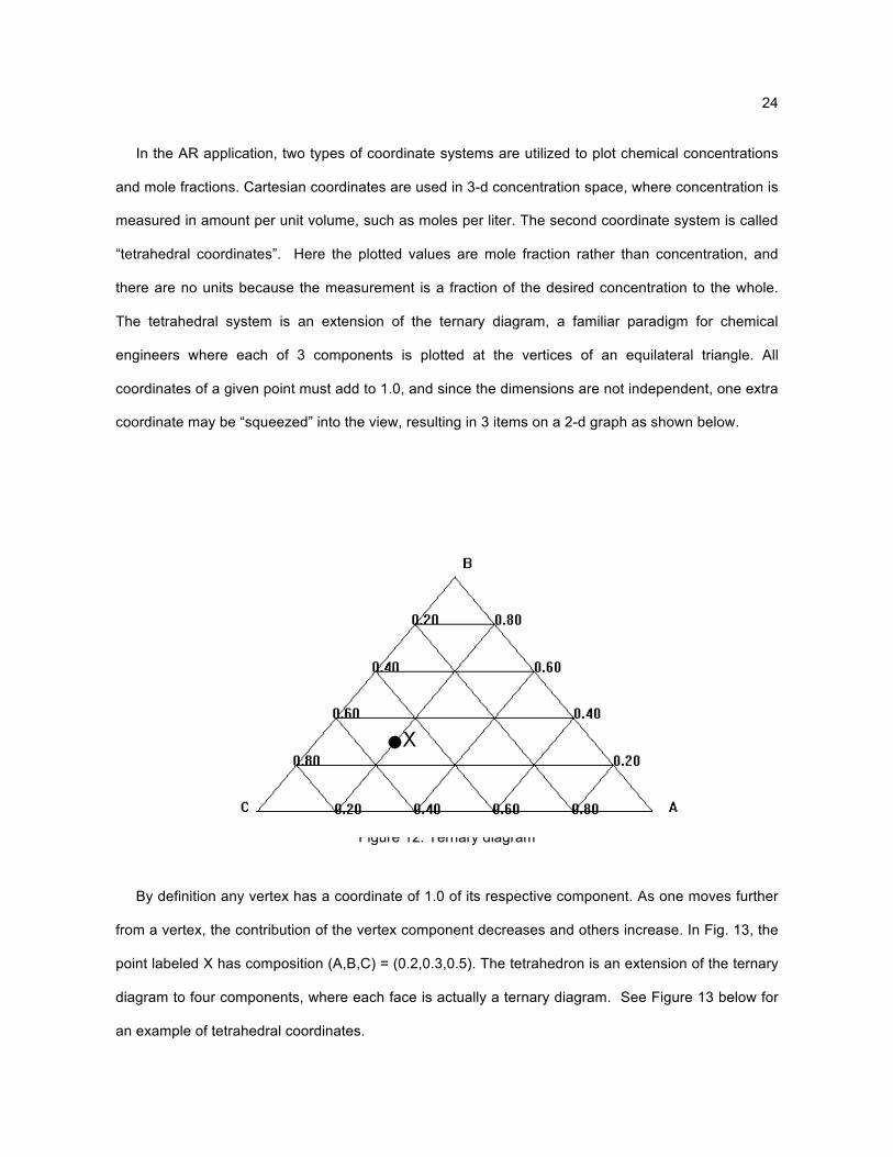
The tetrahedral system is an extension of the ternary diagram, a familiar paradigm for chemical
engineers where each of 3 components is plotted at the vertices of an equilateral triangle. All
coordinates of a given point must add to 1.0, and since the dimensions are not independent, one extra
coordinate may be “squeezed” into the view, resulting in 3 items on a 2-d graph as shown below.
Figure 12. Ternary diagram
By definition any vertex has a coordinate of 1.0 of its respective component. As one moves further
from a vertex, the contribution of the vertex component decreases and others increase. In Fig. 13, the
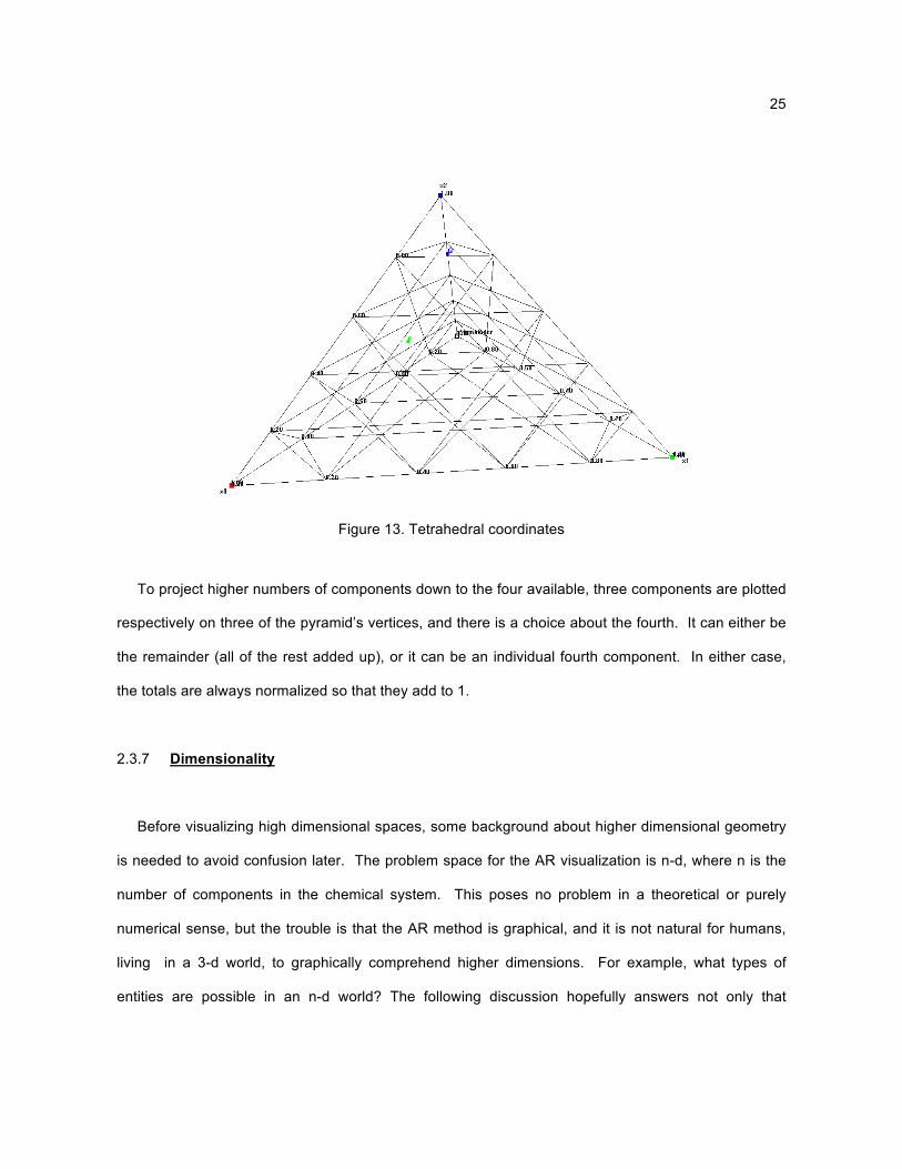
point labeled X has composition (A,B,C) = (0.2,0.3,0.5). The tetrahedron is an extension of the ternary
diagram to four components, where each face is actually a ternary diagram. See Figure 13 below for
an example of tetrahedral coordinates.
25
Figure 13. Tetrahedral coordinates
To project higher numbers of components down to the four available, three components are plotted
respectively on three of the pyramid’s vertices, and there is a choice about the fourth. It can either be
the remainder (all of the rest added up), or it can be an individual fourth component. In either case,
the totals are always normalized so that they add to 1.
2.3.7 Dimensionality
Before visualizing high dimensional spaces, some background about higher dimensional geometry
is needed to avoid confusion later. The problem space for the AR visualization is n-d, where n is the
number of components in the chemical system. This poses no problem in a theoretical or purely
numerical sense, but the trouble is that the AR method is graphical, and it is not natural for humans,
living in a 3-d world, to graphically comprehend higher dimensions. For example, what types of
entities are possible in an n-d world? The following discussion hopefully answers not only that
26
question, but also forms a coherent framework for visualizing objects in any arbitrary number of
dimensions.
First, only 3 different entities are permitted in any world, regardless of dimension:
• Point – a single location in n-d space, P(x0,x1,…xn-1)
• Curve – several points connected together in a path of straight lines; a single line segment is just a
curve with only two points
• Surface – a family of several curves
It will be shown later that the boundary of an AR is of concern and not its interior, so solids are not
included as a fourth entity, thus simplifying the problem. (A solid would be defined as a closed family
of surfaces.) Entities are always finite size, or zero size in the case of points. For example, there are
no lines of infinite length as in Euclidean geometry. Also, notice how each more complex item is built
recursively from a family of simpler items. Therefore, the complex entity may always be replaced with
many simpler ones, if that makes the thought process clearer. For example, the boundary of an AR is
a surface or several surfaces, but this may be considered simply as a large collection of n-d points. If
one can visualize an n-d point, one can visualize an n-d curve and an n-d surface. One final note: the
use of the prefix “hyper”, as it appears in some of the literature (eg. hyper-plane, hyper-surface, etc.) is
avoided in this discussion. It is understood that all spaces are n-d, and calling everything “hyper” adds
nothing new.
Points, curves, and surfaces also have their own dimensionality that is independent of the of the
original concentration problem space. That is, a way is needed to show that a point has no size, a
curve has length, and a surface has length and width. Fortunately, there is a convenient method to do
this, the parametric form. (Thomas and Finney, 1981) Any geometric entity can be defined
parametrically as well as conventionally. For example, think of the familiar definition of a 2-d line.
y=mx+b (among other forms) is a conventional equation, but a parametric equation can also be
27
formed: x = xstart + t * xdir Here x is a vector x(x,y), and t is the parameter. The dimensionality of the
original space has been separated from the dimensionality of the parametric space. In the above
example, x could just as well been 3-d, 4-d, or n-d, and the line would still have one parameter, t. In a
similar way, a surface depends on two parameters; u and v are commonly used. Thus, the following
conventions result.
• Points are parametrically 0-dimensional entities
• Curves are parametrically 1-dimensional entities
• Surfaces are parametrically 2-dimensional entities
Once again, points, curves, and surfaces exist within an n-d concentration space, and the above
definitions do not contradict that, as indicated by the qualifier “parametric”. Using the above
conventions, a surface in n-d is defined as a parametric 2-d collection of curves, which are in turn
parametric 1-d collections of n-d points.
2.3.8 Convex Hulls
Given a set of points in a space, the convex hull is the smallest convex set containing the points. It
is convenient to imagine a convex hull in 3 dimensions, but it is important to realize that convex hulls
can theoretically exist in n-dimensions. The bounding faces of the hull are called “facets”. In the 3d
case, the facets are triangles, but in the general case they are simplices. For reference, background
material on simplices can be found in Bell (Bell, 1987) and Murty (Murty, 1983). There are several
algorithms for computing convex hulls, such as incremental, gift wrap, divide and conquer, and quick
hull. For an overview, the reader may consult Lambert (Lambert, 1998), and Clarkson offers more
detail on the incremental algorithm. (Clarkson, 1993) In the following discussion, reference is made
both to n-d convex hulls (“full hulls”) and 3-d convex hulls (“view-based hulls”). It is important for the
reader to note which type of hull is the subject of discussion, as they serve different purposes.
28
In relation to ARs, there are three uses for convex hulls. First, some AR data-generation
algorithms produce interior points inside the AR as well as border points on the boundary of the AR.
Keep in mind that researchers producing candidate data points cannot visualize them until after the
data are generated and collated into an input data file for the visualizer, by which time their search for
candidate points may have produced both boundary and interior points. In ARs only the boundary is
of interest, so interior points can be filtered out by generating an n-d convex hull and determining
which of the input points are not included in the hull vertices.
Second, a 3-d view-based convex hull can be computed within the visualization and overlaid on the
current 3-d view as a way to check the convexity of the attainable region. By drawing the convex hull
as a semi-transparent “skin”, it can be seen to coincide with the AR. Finally, the third use is to actually
draw the AR surfaces as the 3-d convex hull. This is not needed when data are neatly organized into
curves and surfaces composed of adjacent curves, but becomes necessary when computer
simulations generate data in a disorganized fashion and adjacency information is unavailable.
Convex hull algorithms are a study in themselves. For this reason, previous research by Ken
Clarkson of Bell Laboratories, Murray Hill, New Jersey is utilized. (Clarkson et al., 1993) Mr. Clarkson
generously provides a complete stand-alone open-source application for computing convex hulls in
general numbers of dimensions, downloadable from (Clarkson, 2003). Clarkson’s algorithm is an
incremental one that grows the convex hull one point at a time. The basic data structure for storing
the hull is a splay tree. Splay trees are binary trees that maintain an average or amortized cost per
operation of O(logN) through a succession of tree node rotations that keep recently accessed nodes
near the top of the tree and also maintain a roughly balanced tree structure. (Weiss, 1999)
29
2.4 Attainable Regions
The application domain of this project is attainable regions or ARs, so some background
information in chemical reactor design and ARs is necessary before proceeding further. The AR is a
tool to solve the general problem of chemical reactor design synthesis, or the problem of determining
some combination of different types of chemical reactors to achieve a desired output. In practice,
chemical systems are not limited to just one operation or type of reactor. There are three common
types of ideal reactors plus mixing, and they can be combined in an infinite number of combinations
through series, parallel, bypass, looping, etc., so clearly it is a large problem.
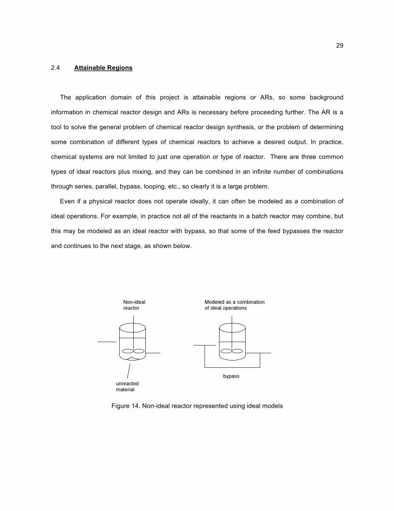
Even if a physical reactor does not operate ideally, it can often be modeled as a combination of
ideal operations. For example, in practice not all of the reactants in a batch reactor may combine, but
this may be modeled as an ideal reactor with bypass, so that some of the feed bypasses the reactor
and continues to the next stage, as shown below.
Figure 14. Non-ideal reactor represented using ideal models
30
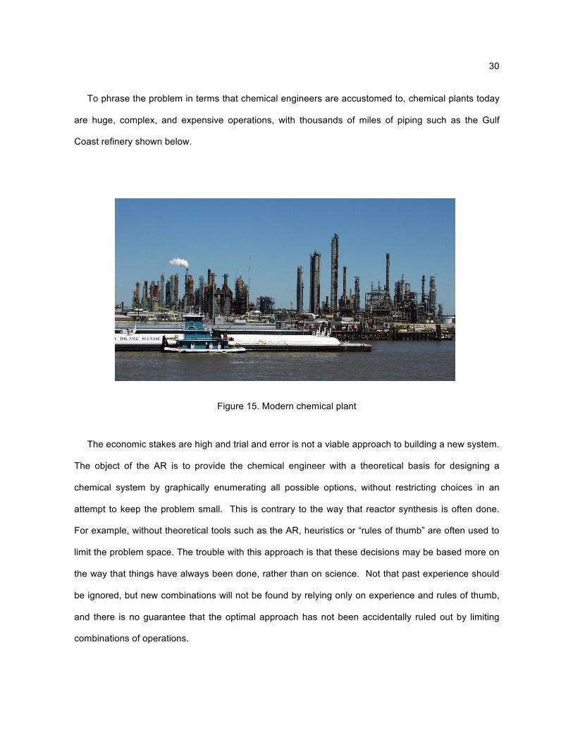
To phrase the problem in terms that chemical engineers are accustomed to, chemical plants today
are huge, complex, and expensive operations, with thousands of miles of piping such as the Gulf
Coast refinery shown below.
Figure 15. Modern chemical plant
The economic stakes are high and trial and error is not a viable approach to building a new system.
The object of the AR is to provide the chemical engineer with a theoretical basis for designing a
chemical system by graphically enumerating all possible options, without restricting choices in an
attempt to keep the problem small. This is contrary to the way that reactor synthesis is often done.
For example, without theoretical tools such as the AR, heuristics or “rules of thumb” are often used to
limit the problem space. The trouble with this approach is that these decisions may be based more on
the way that things have always been done, rather than on science. Not that past experience should
be ignored, but new combinations will not be found by relying only on experience and rules of thumb,
and there is no guarantee that the optimal approach has not been accidentally ruled out by limiting
combinations of operations.
31
A more scientific method is desired. The first step to finding an optimal system is to determine the
space of all possible systems. Then, the optimal or desired solution can be selected from that solution
space. The AR is this space of possible combinations, and represents a volume or solid in n-space,
where n is the number of chemical components in the system. This first step is of interest in this work,
finding the space of all possibilities or AR, and in particular visualizing what that space looks like. The
second step, using the AR to identify the desired state and an optimal path to reach that state, can still
be a complicated optimization problem and is beyond the scope of this work, but the AR at least
defines the possibilities. In the following sections, specific features of the AR are described in more
detail.
2.4.1 Attainable Region Theory
Attainable regions are not a new idea; Horn first described in 1964 the idea of the set of all possible
solutions to chemical reactor synthesis problems, which he called the attainable region. (Horn, 1964)
His definition of the AR was quite broad in the sense that he included as variables reactor
concentrations, holding time, pressure, temperature, economics, etc. This thesis closely follows the
more limited definitions of the AR proposed by later authors such as Glasser, Hildebrandt, and
Feinberg, where the AR is restricted to the possible set of reactor concentrations in isothermal
reactors involving mixtures of constant density, operating at steady state conditions. (Feinberg and
Hildebrandt, 1997; Glasser, et. al., 1987) Four different unit operations are allowed, three of which are
types of ideal reactors and the fourth is bulk mixing; all are described in the following sections.
It should be noted that these assumptions are not overly restrictive; many chemical processes are
performed using these four operations and under these conditions. Keep in mind that the unit
operations can be combined in any conceivable arrangement. On the other hand, processes such as
distillation, separation, and other conditions are not included in this work, and perhaps the scope of
32
future work will be to expand the generality of the method more closely to what Horn originally
envisioned.
2.4.2 Terminology and Definitions
Consider the concentration vector at any point in the system as an n-dimensional vector of
individual component concentrations c(c0, c1, c2,…, cn-1) where ci is the concentration of the (i+1)th
component of the system in moles per liter. (Vector quantities are denoted with a bold font.)
Graphically, the component compositions directly map to coordinates or dimensions in a coordinate
system. Let the rate of change of concentration be defined also as a vector, called the rate vector,
r(c), in units of moles reacted per unit volume per unit time. Lastly, define residence time or " as the
time that the reacting material spends inside the reactor; units are typical units of time such as
seconds, hours, etc. Finally, concentration and residence time are related, as the concentration within
a reactor changes over time, ie., current concentration is a function of residence time, c = f(").
2.4.3 Fundamental Reactor Types and Operations
Three types of ideal reactors plus bulk mixing are allowed for a total of 4 fundamental operations.
The following description is a very brief overview of these operations, but the reader is encouraged to
consult a chemical reactor design textbook such as Fogler (Fogler, 1999) for a complete reference.
Although attainable regions have been applied to other types of systems such as separations, (Nisoli
et. al., 1997) this thesis is limited to the following:
Plug-flow reactor (PFR)
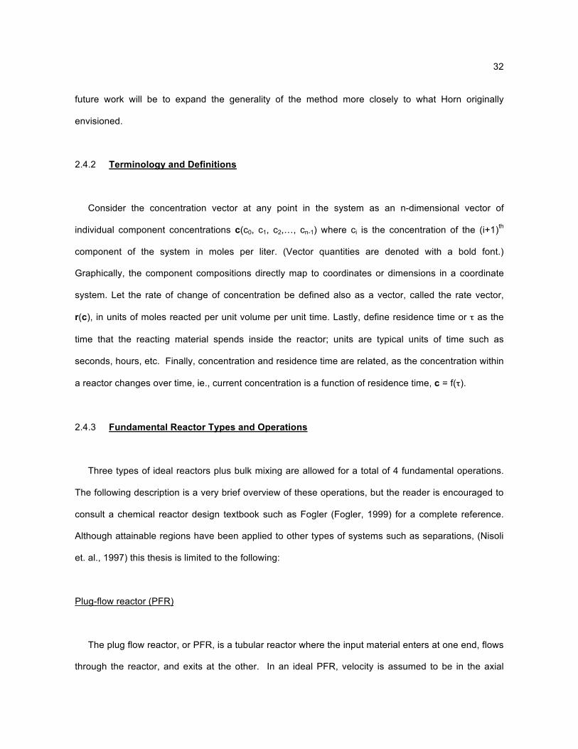
The plug flow reactor, or PFR, is a tubular reactor where the input material enters at one end, flows
through the reactor, and exits at the other. In an ideal PFR, velocity is assumed to be in the axial
33
direction only, and all quantities to be constant in all other directions. The flow is modeled as turbulent
plug flow as the name implies, and the PFR is usually diagrammed as shown below.
Figure 16. Plug flow reactor
The PFR is usually modeled by the following differential equation that is integrated along the length of
the reactor to determine the concentration at any point along the reactor:
dc/d" = r(c)
where c is the output concentration vector, r(c) is the reaction rate vector, and " is the residence time,
which in the PFR is the time it takes one unit of material (eg., one atom) just entering the reactor to
make its way to the exit. In an ideal PFR, " is the same for all atoms of the material at a given
position.
Differential side-stream reactor (DSR)
34
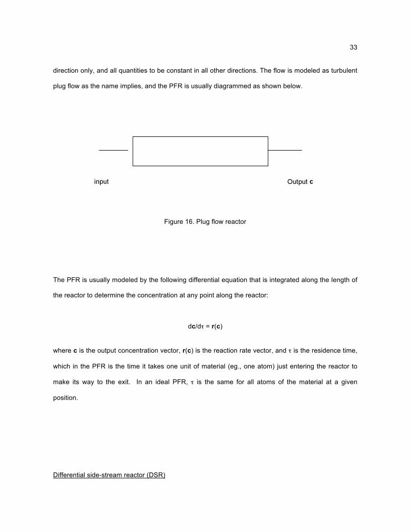
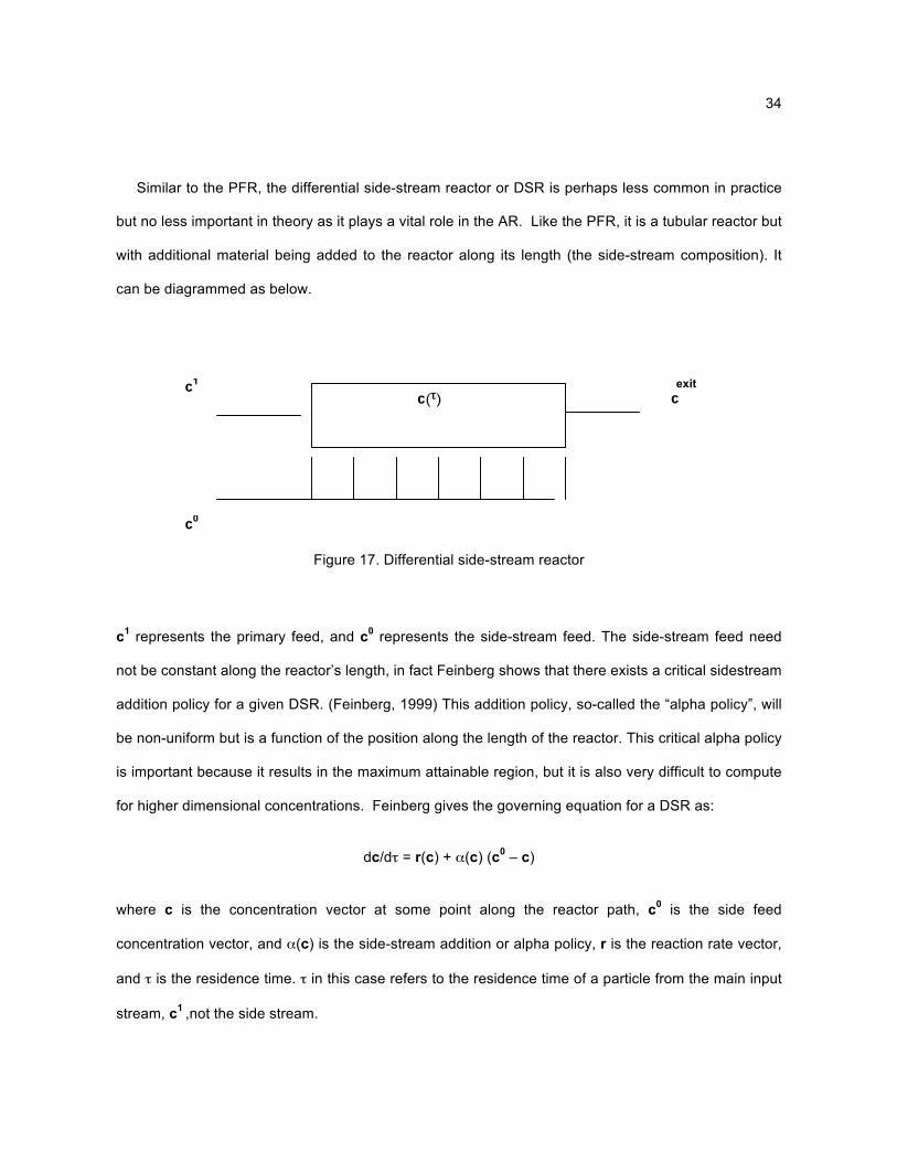
Similar to the PFR, the differential side-stream reactor or DSR is perhaps less common in practice
but no less important in theory as it plays a vital role in the AR. Like the PFR, it is a tubular reactor but
with additional material being added to the reactor along its length (the side-stream composition). It
can be diagrammed as below.
Figure 17. Differential side-stream reactor
c1 represents the primary feed, and c0 represents the side-stream feed. The side-stream feed need
not be constant along the reactor’s length, in fact Feinberg shows that there exists a critical sidestream
addition policy for a given DSR. (Feinberg, 1999) This addition policy, so-called the “alpha policy”, will
be non-uniform but is a function of the position along the length of the reactor. This critical alpha policy
is important because it results in the maximum attainable region, but it is also very difficult to compute
for higher dimensional concentrations. Feinberg gives the governing equation for a DSR as:
dc/d" = r(c) + #(c) (c0 – c)
where c is the concentration vector at some point along the reactor path, c0 is the side feed
concentration vector, and #(c) is the side-stream addition or alpha policy, r is the reaction rate vector,
and " is the residence time. " in this case refers to the residence time of a particle from the main input
stream, c1 ,not the side stream.
exit
35
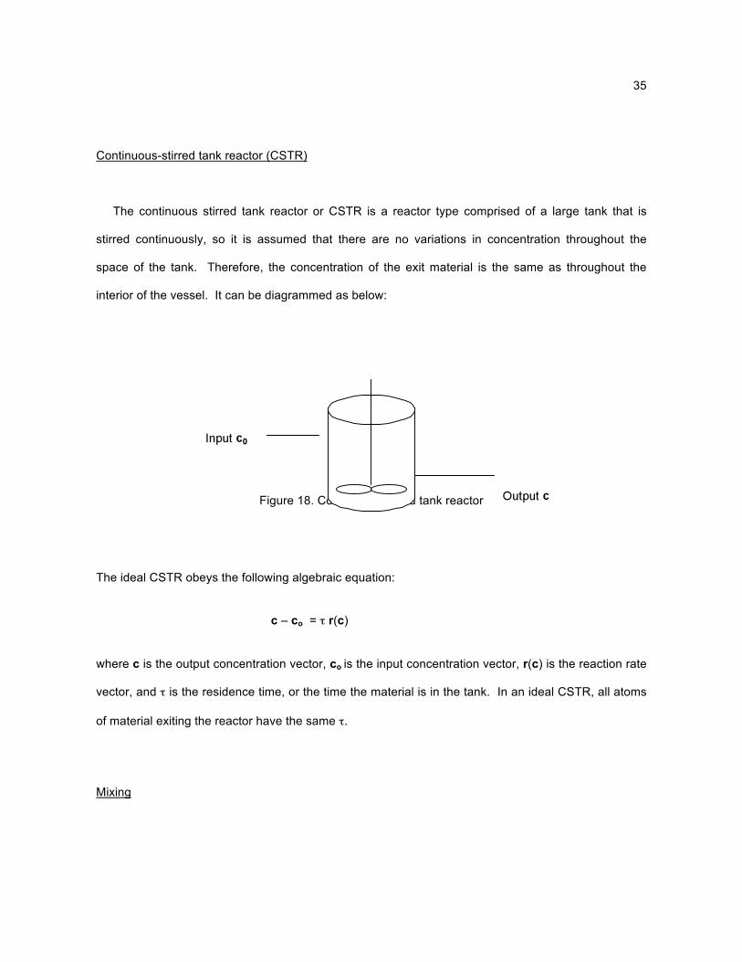
Continuous-stirred tank reactor (CSTR)
The continuous stirred tank reactor or CSTR is a reactor type comprised of a large tank that is
stirred continuously, so it is assumed that there are no variations in concentration throughout the
space of the tank. Therefore, the concentration of the exit material is the same as throughout the
interior of the vessel. It can be diagrammed as below:
Figure 18. Continuous stirred tank reactor
The ideal CSTR obeys the following algebraic equation:
c – co = " r(c)
where c is the output concentration vector, co is the input concentration vector, r(c) is the reaction rate
vector, and " is the residence time, or the time the material is in the tank. In an ideal CSTR, all atoms
of material exiting the reactor have the same ".
Mixing
36
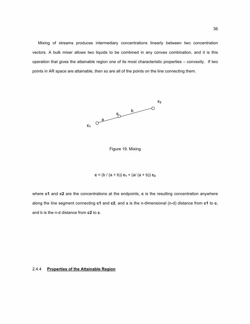
Mixing of streams produces intermediary concentrations linearly between two concentration
vectors. A bulk mixer allows two liquids to be combined in any convex combination, and it is this
operation that gives the attainable region one of its most characteristic properties – convexity. If two
points in AR space are attainable, then so are all of the points on the line connecting them.
Figure 19. Mixing
c = (b / (a + b)) c1 + (a/ (a + b)) c2
where c1 and c2 are the concentrations at the endpoints, c is the resulting concentration anywhere
along the line segment connecting c1 and c2, and a is the n-dimensional (n-d) distance from c1 to c,
and b is the n-d distance from c2 to c.
2.4.4 Properties of the Attainable Region
37
All of the groundwork is now in place to form an attainable region. The AR is the closed volume in
n-dimensional space representing all of the possible (attainable) chemical compositions that can be
produced by the chemical system, given some starting feed composition. In evaluating a candidate
AR, all of the following test conditions must necessarily hold in order for the AR to be valid. (Feinberg
and Hildebrandt, 1997)
• The boundary must be convex, since mixing can fill in any concavity.
• No rate vectors on the boundary may point outward from the AR. They must either be zero, or
tangent to the boundary, or point inward. If a rate vector from any point on the AR boundary were
to point outward, the AR would have to be extended (grown) because a new, larger AR would be
possible.
• No rate vectors in the complement of the AR, when extrapolated backwards, may intercept the AR
(known as the complement principle). If such a rate vector were to exist, its base point could be
reached from the boundary of the existing AR with a suitable CSTR, again growing the AR.
To summarize, the AR represents the largest possible volume formed by the chemical
compositions of the given system, since it represents all possible compositions that are attainable. If
there is any operation that can make the AR grow larger, then it must grow in order to be valid. The
above properties are three ways that this can happen. One final note: the AR represents operations in
the theoretical limit. For example, a point may be attainable through an infinitely long PFR. Although
in practice this is impossible, it is possible to come arbitrarily close through a sufficiently long PFR.
2.4.5 Features of the Attainable Region
38
Let us now further characterize an AR by the following features, according to Feinberg. (Feinberg
and Hildebrandt, 1997)
• The boundary of the AR is a 2d parametric surface, or a collection of such surfaces.
• The boundary determines the AR and vice versa, ie., the boundary is of interest rather than the
interior.
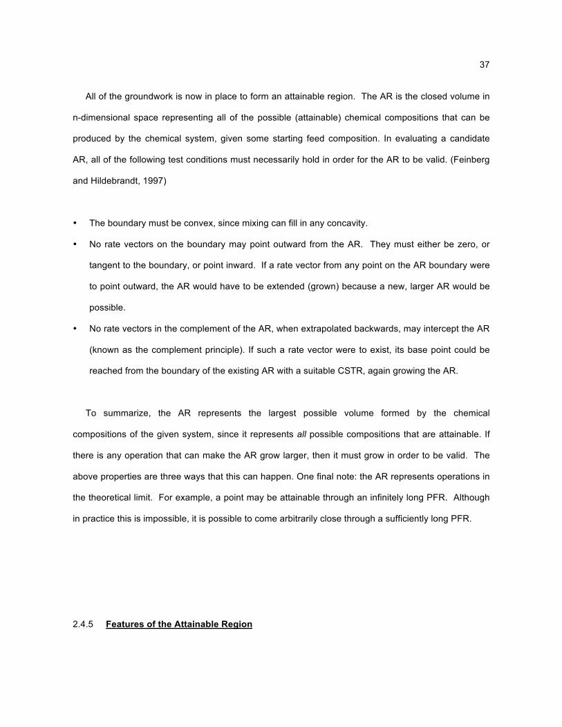
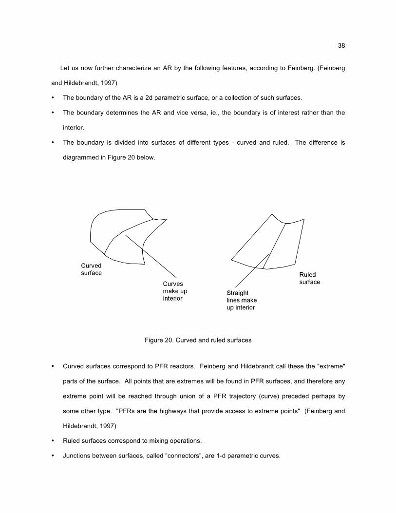
• The boundary is divided into surfaces of different types - curved and ruled. The difference is
diagrammed in Figure 20 below.
Figure 20. Curved and ruled surfaces
• Curved surfaces correspond to PFR reactors. Feinberg and Hildebrandt call these the "extreme"
parts of the surface. All points that are extremes will be found in PFR surfaces, and therefore any
extreme point will be reached through union of a PFR trajectory (curve) preceded perhaps by
some other type. "PFRs are the highways that provide access to extreme points" (Feinberg and
Hildebrandt, 1997)
• Ruled surfaces correspond to mixing operations.
• Junctions between surfaces, called "connectors", are 1-d parametric curves.

39
• Sharp connectors (adjacent surfaces not tangent) correspond to PFRs (no mixing, only reacting).
• Smooth connectors (adjacent surfaces tangent) correspond to DSRs (mixing and reacting
simultaneously).
• Endpoints of DSR connectors (smooth) correspond to CSTRs.
These features are evident in the results of sample problem 1; see Section 4.2. One of the
objectives of the AR visualization is to visually verify a candidate AR for validity. Functions built into
the program such as pan, zoom, rotate, coordinate system settings, and convex hulls permit the
critical viewing of the AR and the ability to quickly and easily spot the above features. When viewing
sample problem 1, it is instructive to refer back to this list and look for all of these features in the AR.
2.4.6 Current Attainable Region Visualizations
A survey of relatively recent AR literature reveals that visualization in general lags behind other
aspects of AR research such as theory, algorithms, numerical methods, etc. The following literature
review is not intended to be a criticism of publications in any way. It is however intended to be a
justification of the need for better visualization techniques in the AR field. As a direct example of this
fact, consider the following correspondence from a collaborator in South Africa. “I am currently
developing algorithms for higher AR and have 3D and 4D results. I am struggling with the 4D
interpretation, not easy without visualization!” (Seodigeng, 2002, personal communication)
Table I below summarizes eleven AR research papers published in recent years. Current research
is focused in a few locations: University of Witwatersrand in Johannesburg, South Africa, Carnegie
Mellon University in Pittsburgh Pennsylvania, University of Rochester in Rochester New York, and
University of Massachusetts in Amherst Massachusetts. A few trends stand out. First, the most
popular visualization method is still the 2-d line graph. Second, another common approach is to
discard dimensions altogether from a visualization, usually accompanied by an explanation that only
40
certain dimensions are of interest. For example, Feinberg and Hildebrandt write: “We shall suppose
that A2 and A3 are desirable products and that species A4 has no value.” (Feinberg and Hildebrandt,
1997) Thus, A4 is not plotted in resulting visualizations and a 4-d problem is displayed in 3-d. Finally,
the third approach is to not visualize the results at all in the publication. Even in these cases, a
sample problem of a certain dimension is discussed, but results are not displayed graphically.
In the majority of cases tabulated below, the dimensionality of the visualization is less than the
dimensionality of the sample problem. This is a contradiction in philosophy to the AR method, which is
inherently n-d. The basis for ARs is to display the space of all possible compositions in n-d space. If
results are displayed in a reduced space, (for whatever reason) then all possibilities are not visible,
reducing the efficacy of the AR method. It must be noted that there is a significant difference between
“temporary” dimension reduction on a per view basis, and “permanent” dimension reduction for an
entire visualization. The former case is indeed what is utilized in the AR visualization developed for
this thesis. A variety of views with different combinations of dimensions can be produced because all
dimensions are stored internally and subsets are viewed at any one time. The latter case involves
reducing dimensionality from the outset and only visualizing certain dimensions. In all of the
dimension-reduced visualizations below, no other views of different combinations of dimensions exist,
indicating that “permanent” reduction has occurred. One final footnote is that none of the AR literature
surveyed utilized tetrahedral coordinates as a display paradigm.
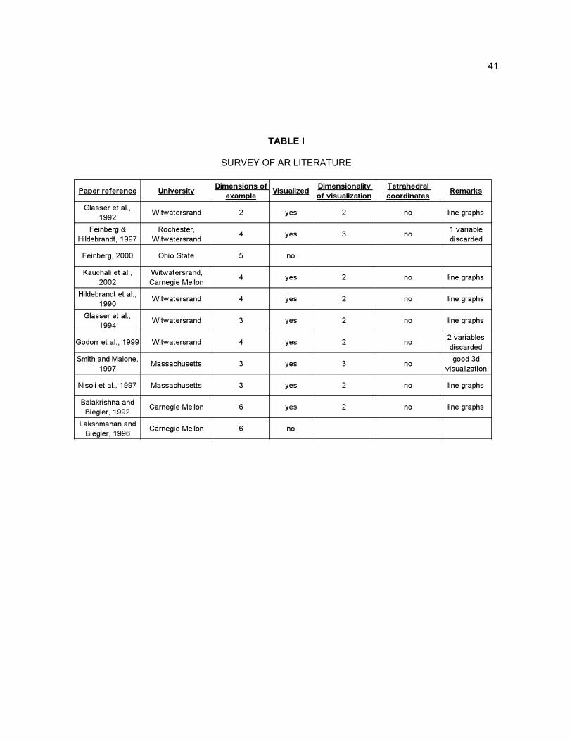
41
TABLE I
SURVEY OF AR LITERATURE
42
3. APPLICATION DEVELOPMENT
Many concepts developed in the previous chapter are implemented during the course of
developing a working computer application including dimension reduction, various coordinate systems,
and convex hulls. Other application features are explored in this chapter for the first time, such as
surface rendering, data probing, and development of a standard input file format.
3.1 Introduction
The synthesis of background knowledge from computer science, scientific visualization, and
chemical engineering is demonstrated through a working computer program. Two purposes are
served by the application development: to gain knowledge and to share knowledge with others.
Through collaboration with working researchers in ARs, one goal is to actually help someone else
solve a real visualization problem. In this way, not only is knowledge personally gained, but the
enhancement of the current state of AR visualization is shared through a scientific community for the
benefit of all.
The sections in this chapter may be roughly divided into two categories. The first group, Sections
3.2 through Sections 3.7, describe the implementation of the major contributions of this thesis to the
current state of AR visualization and closely relate to the background issues presented in the previous
chapter. The second group, Sections 3.8 through Sections 3.11, are a discussion of some of the
practical problems that had to be solved in order for the major contributions to become a reality. This
group of topics tends to be more specific to computer graphics and somewhat less specific to ARs. It
should be noted that while this second group is less theoretical in nature, research was still done into
various ways of accomplishing these tasks. This research is documented within these sections rather
than separately in the background chapter.
43
The application is an interactive viewer that allows an AR data file to be read in and viewed in real-
time 3d graphics. Choices of coordinate systems (orthogonal and tetrahedral) are available as well as
the ability to selectively view 3 or 4 dimensions out of any general number. The program includes
interactive viewing controls such as panning, rotating, and zooming, and includes realistic lighting and
shading of surfaces. Querying of the data is available through a data probing algorithm; various other
controls and options are available such as color choices, labels, etc. Through the use, with permission,
of open-source code for computing convex hulls, the program integrates a convex hull computation
feature. A data file format was developed for the input of AR data to the program, and is documented
in Appendix A. Finally, an “offline” pre-processing utility was written to accept large data sets and filter
out extraneous data.
44
3.2 Platforms
At EVL, there exist a variety of computer graphics and virtual reality hardware and software,
including two CAVEs, so some choices had to be made about hardware and software platforms. As
can happen, these decisions changed a few times during the course of development. The initial
design was to develop a CAVE-based application running under the CAVE Library, on Silicon
Graphics machines (IRIX 6.5) and written in C++ and OpenGL. Initial expectations were to gain an
advantage in high dimensional visualization through the use of a high-end virtual reality system such
as the CAVE. Development proceeded in this direction for several months, then a gradual migration
occurred toward a PC Windows-based application.
The reasons are several. From the onset, most of the development was actually done on a
Windows laptop running a console-based application that closely resembled the CAVE program. (A
console application in Windows terminology is an application that runs in a DOS-like console window,
similar to a UNIX console, without any of the Windows GUI features such as menus, dialog boxes,
etc.) In this way code was written offline and offsite, and each week ported and tested in the CAVE.
This continued for several months, and the user interface primarily consisted of pressing wand buttons
in the CAVE. In CAVE terminology, the “wand” is a tracked “3d mouse” with five buttons and a
joystick. (Some wand versions have only three buttons and a joystick or trackball.) Navigation is
performed by pointing the wand and operating the joystick, and features are selected by pressing the
various buttons.
Several ideas slowly evolved. First, testing became more frequent on the Windows console and
less frequent in the CAVE, primarily because the laptop could be conveniently set up wherever it was
needed, rather than making a trip down to the CAVE, sometimes to find it unavailable, etc. This
convenience made it clear that a full-fledged Windows application complete with GUI items such as
menus, dialog boxes, and online help would be more accessible than a CAVE program, especially
considering that the goal was to collaborate with other researchers who most likely would not have
45
access to CAVE hardware. Of course, the console application used for initial development had none
of those GUI elements, and a good deal of work would be required to build one.
At the same time, the interface elements provided by the CAVE, primarily the wand buttons,
became too restrictive. When the program was new and the list of features small, five wand buttons
were sufficient, but as features were added the burden on the user became to remember which button
or combination of buttons did what. A logical step would have been to display user interface elements
within the display space of the CAVE, such as menus and to select menu items by pointing at them
with the wand. However, the CAVE system, to the best of our knowledge, does not provide any tools
for building standardized user interface elements, as does Windows, or XWindows (the window
system under most UNIX operating systems).
That is not to say that GUI elements have not been programmed for the CAVE before; many have
been developed during the course of prior work. However, they are all project-specific and not general
purpose enough to re-use easily. What is required is a set of GUI building tools such as Microsoft’s
MFC for Windows, or FLTK for Linux. Recall from Section 2.2.3 that building tools are an essential
part of a modern user interface. Without them, all elements would have to be programmed in OpenGL
from “scratch”. Anyone who has ever done this knows that it rapidly becomes a project in itself,
quickly consuming the majority of the application’s code. While user interface design is certainly a
part of this thesis, it is not intended to become the focus of the work.
The last reason for the switch to a PC application is the growing trend to find economical graphics
cards on PCs that rival or surpass the highest-end graphics machines of just a few years ago.
Spurred by the computer games industry, high-speed realistic computer graphics can be found on just
about any commodity PC, or upgraded for a hundred dollars or so. In general, even at our own EVL
lab, the trend seems to be moving toward PCs and PC clusters, both Windows and Linux, and the
Silicon Graphics dedicated graphics machines tend to be used less and less.
46
That is not to say that a PC is the only intended platform for the AR visualization. Future plans are
to utilize a tiled display, either monoscopic (2-d) or auto-stereo (3-d) to display results. Recall from
Sections 2.1.2 and 2.1.3, that both of these devices provide wide field of view and high resolution,
making them primary candidates for this type of scientific visualization. Another advantage is the fact
that the tiled nature of the displays lends itself to showing multiple views simultaneously, one per tile if
desired. The program architecture described in the following section is designed to be scalable to
multiple views. The final advantage that both of these systems have over the CAVE is the availability
of a master display, keyboard, and mouse nearby to the tiled display which can function as a “control
panel” over the application. On the other hand, in a CAVE setup, this workstation is outside of the
CAVE and the user has to remove VR hardware and exit the CAVE to access it.
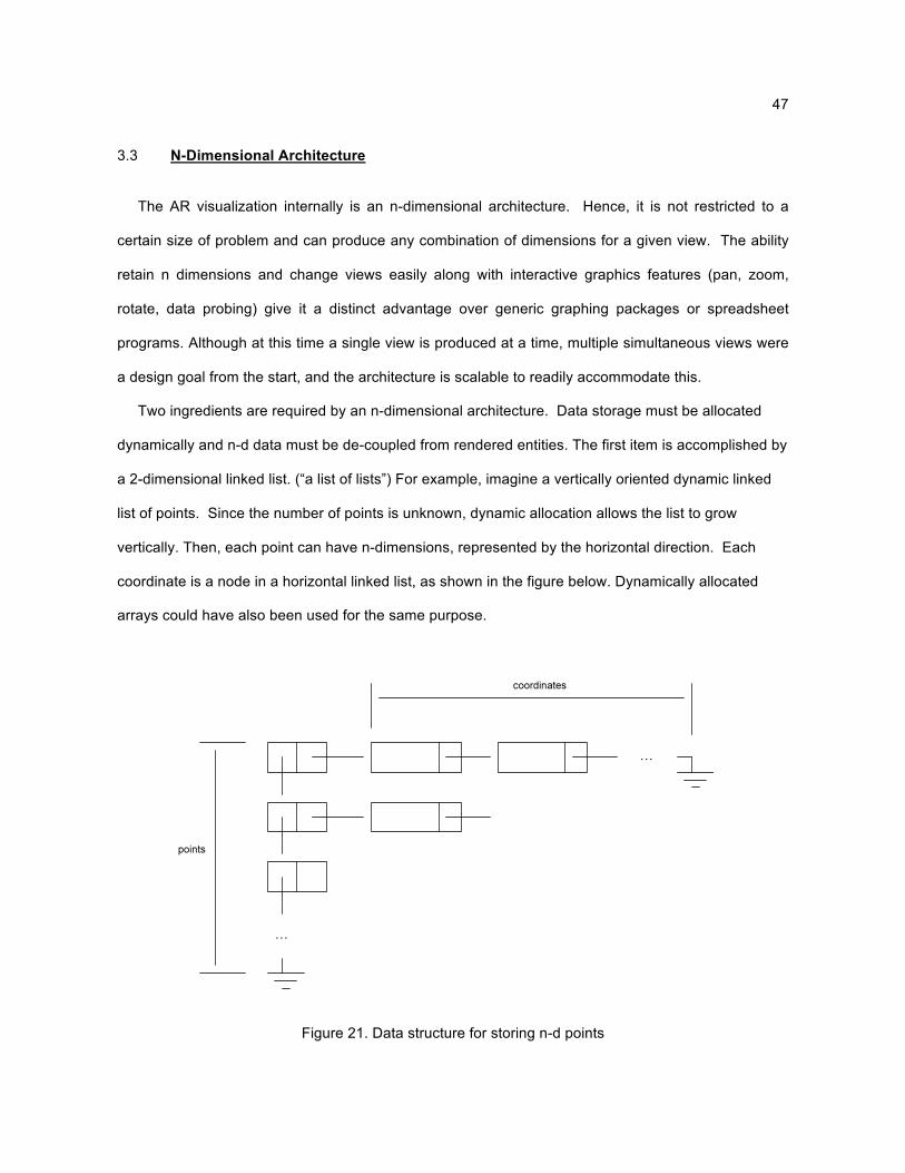
47
3.3 N-Dimensional Architecture
The AR visualization internally is an n-dimensional architecture. Hence, it is not restricted to a
certain size of problem and can produce any combination of dimensions for a given view. The ability
retain n dimensions and change views easily along with interactive graphics features (pan, zoom,
rotate, data probing) give it a distinct advantage over generic graphing packages or spreadsheet
programs. Although at this time a single view is produced at a time, multiple simultaneous views were
a design goal from the start, and the architecture is scalable to readily accommodate this.
Two ingredients are required by an n-dimensional architecture. Data storage must be allocated
dynamically and n-d data must be de-coupled from rendered entities. The first item is accomplished by
a 2-dimensional linked list. (“a list of lists”) For example, imagine a vertically oriented dynamic linked
list of points. Since the number of points is unknown, dynamic allocation allows the list to grow
vertically. Then, each point can have n-dimensions, represented by the horizontal direction. Each
coordinate is a node in a horizontal linked list, as shown in the figure below. Dynamically allocated
arrays could have also been used for the same purpose.
Figure 21. Data structure for storing n-d points
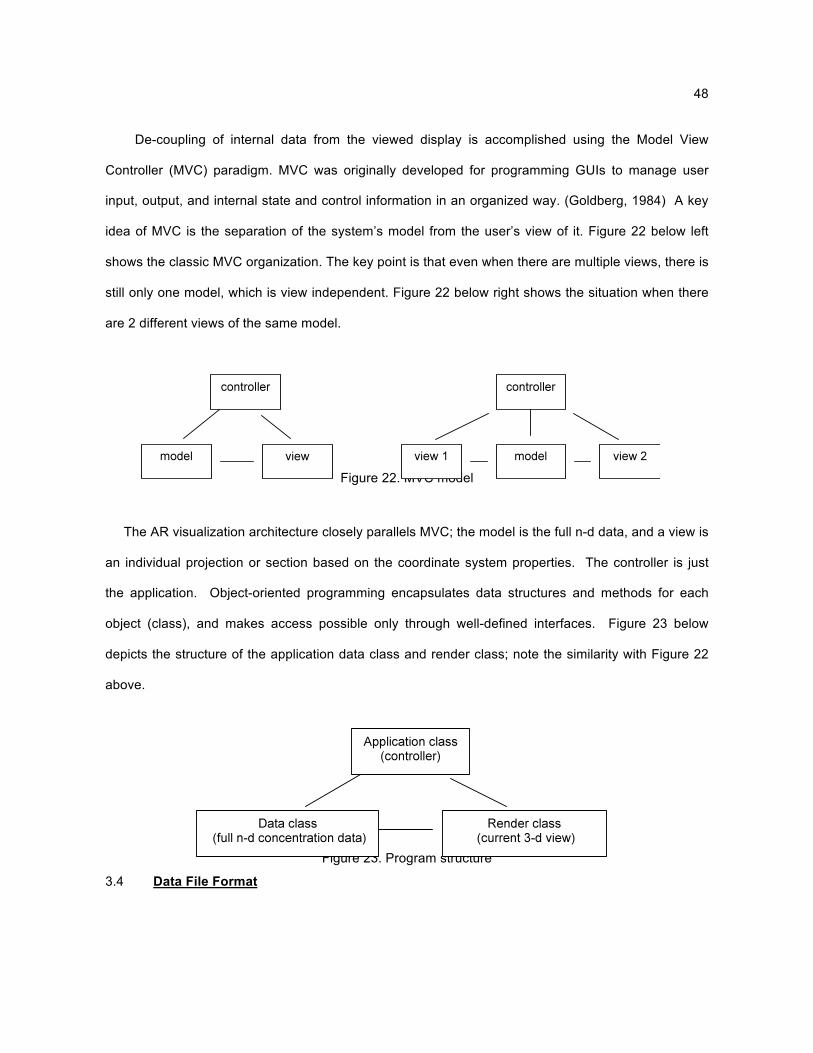
48
De-coupling of internal data from the viewed display is accomplished using the Model View
Controller (MVC) paradigm. MVC was originally developed for programming GUIs to manage user
input, output, and internal state and control information in an organized way. (Goldberg, 1984) A key
idea of MVC is the separation of the system’s model from the user’s view of it. Figure 22 below left
shows the classic MVC organization. The key point is that even when there are multiple views, there is
still only one model, which is view independent. Figure 22 below right shows the situation when there
are 2 different views of the same model.
Figure 22. MVC model
The AR visualization architecture closely parallels MVC; the model is the full n-d data, and a view is
an individual projection or section based on the coordinate system properties. The controller is just
the application. Object-oriented programming encapsulates data structures and methods for each
object (class), and makes access possible only through well-defined interfaces. Figure 23 below
depicts the structure of the application data class and render class; note the similarity with Figure 22
above.
Figure 23. Program structure
3.4 Data File Format
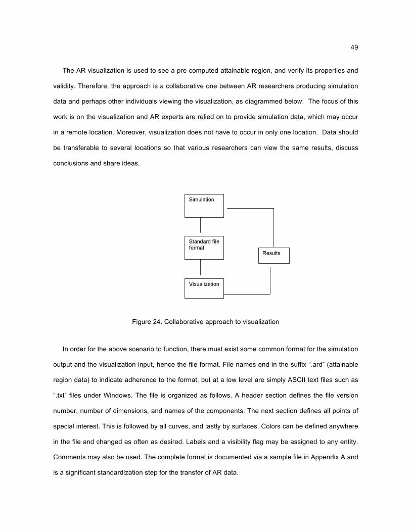
49
The AR visualization is used to see a pre-computed attainable region, and verify its properties and
validity. Therefore, the approach is a collaborative one between AR researchers producing simulation
data and perhaps other individuals viewing the visualization, as diagrammed below. The focus of this
work is on the visualization and AR experts are relied on to provide simulation data, which may occur
in a remote location. Moreover, visualization does not have to occur in only one location. Data should
be transferable to several locations so that various researchers can view the same results, discuss
conclusions and share ideas.
Figure 24. Collaborative approach to visualization
In order for the above scenario to function, there must exist some common format for the simulation
output and the visualization input, hence the file format. File names end in the suffix “.ard” (attainable
region data) to indicate adherence to the format, but at a low level are simply ASCII text files such as
“.txt” files under Windows. The file is organized as follows. A header section defines the file version
number, number of dimensions, and names of the components. The next section defines all points of
special interest. This is followed by all curves, and lastly by surfaces. Colors can be defined anywhere
in the file and changed as often as desired. Labels and a visibility flag may be assigned to any entity.
Comments may also be used. The complete format is documented via a sample file in Appendix A and
is a significant standardization step for the transfer of AR data.

50
The format is relatively new (version 1.0) and is still subject to revision through ongoing research.
Hopefully one day it may evolve into a standard that all AR simulation programs will write to. As a
courtesy to other researchers, outside data was temporarily accepted in any format (eg. multiple
smaller files of columnar spreadsheet data) and then parsed and collected it into one “.ard” file. This
was done by a combination of text editing and writing small utility parsing programs to help create the
final data file. It is expected that in the future AR researchers will perform this process locally, collating
their data into a file according to the standard.
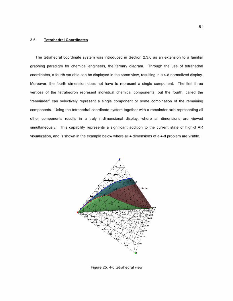
51
3.5 Tetrahedral Coordinates
The tetrahedral coordinate system was introduced in Section 2.3.6 as an extension to a familiar
graphing paradigm for chemical engineers, the ternary diagram. Through the use of tetrahedral
coordinates, a fourth variable can be displayed in the same view, resulting in a 4-d normalized display.
Moreover, the fourth dimension does not have to represent a single component. The first three
vertices of the tetrahedron represent individual chemical components, but the fourth, called the
“remainder” can selectively represent a single component or some combination of the remaining
components. Using the tetrahedral coordinate system together with a remainder axis representing all
other components results in a truly n-dimensional display, where all dimensions are viewed
simultaneously. This capability represents a significant addition to the current state of high-d AR
visualization, and is shown in the example below where all 4 dimensions of a 4-d problem are visible.
Figure 25. 4-d tetrahedral view
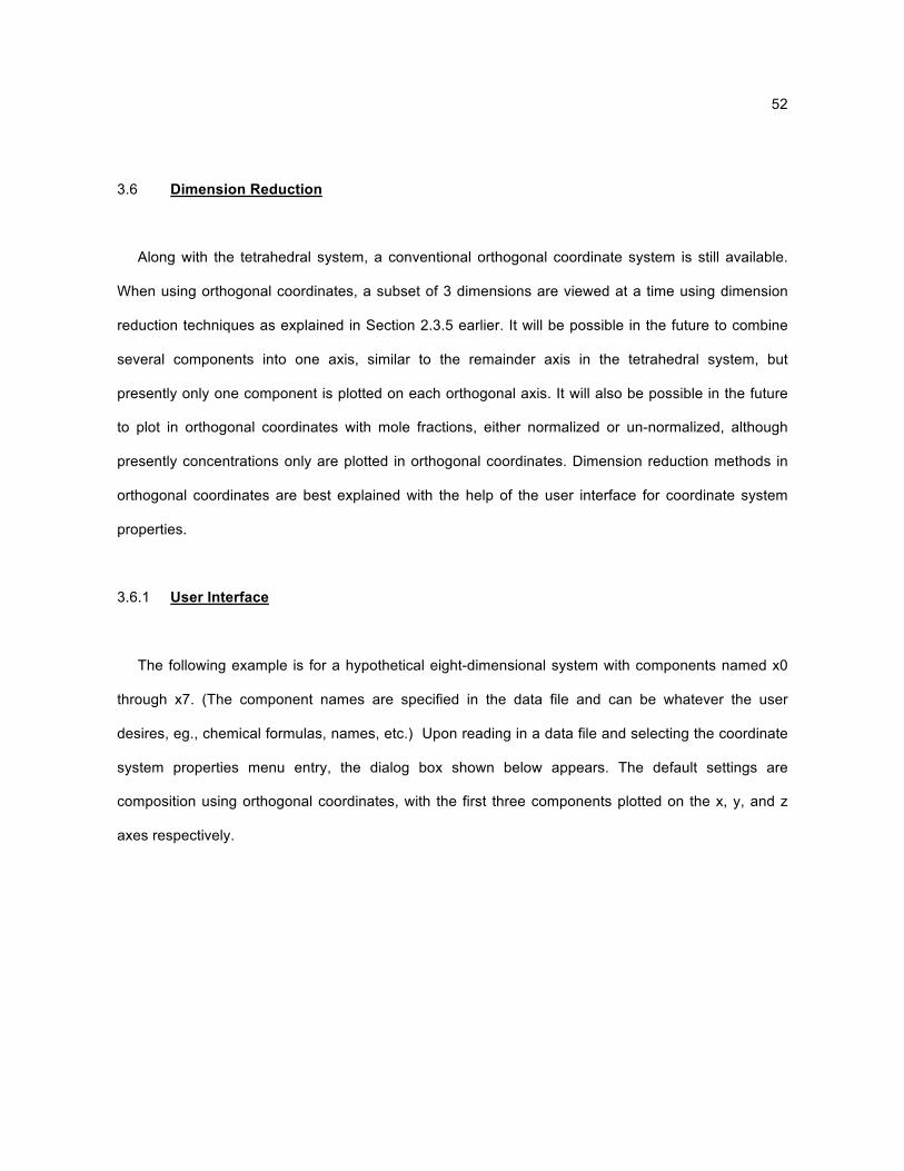
52
3.6 Dimension Reduction
Along with the tetrahedral system, a conventional orthogonal coordinate system is still available.
When using orthogonal coordinates, a subset of 3 dimensions are viewed at a time using dimension
reduction techniques as explained in Section 2.3.5 earlier. It will be possible in the future to combine
several components into one axis, similar to the remainder axis in the tetrahedral system, but
presently only one component is plotted on each orthogonal axis. It will also be possible in the future
to plot in orthogonal coordinates with mole fractions, either normalized or un-normalized, although
presently concentrations only are plotted in orthogonal coordinates. Dimension reduction methods in
orthogonal coordinates are best explained with the help of the user interface for coordinate system
properties.
3.6.1 User Interface
The following example is for a hypothetical eight-dimensional system with components named x0
through x7. (The component names are specified in the data file and can be whatever the user
desires, eg., chemical formulas, names, etc.) Upon reading in a data file and selecting the coordinate
system properties menu entry, the dialog box shown below appears. The default settings are
composition using orthogonal coordinates, with the first three components plotted on the x, y, and z
axes respectively.
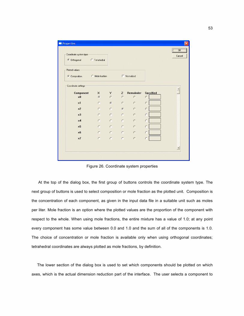
53
Figure 26. Coordinate system properties
At the top of the dialog box, the first group of buttons controls the coordinate system type. The
next group of buttons is used to select composition or mole fraction as the plotted unit. Composition is
the concentration of each component, as given in the input data file in a suitable unit such as moles
per liter. Mole fraction is an option where the plotted values are the proportion of the component with
respect to the whole. When using mole fractions, the entire mixture has a value of 1.0; at any point
every component has some value between 0.0 and 1.0 and the sum of all of the components is 1.0.
The choice of concentration or mole fraction is available only when using orthogonal coordinates;
tetrahedral coordinates are always plotted as mole fractions, by definition.
The lower section of the dialog box is used to set which components should be plotted on which
axes, which is the actual dimension reduction part of the interface. The user selects a component to
54
plot on each of the X,Y,and Z axes. Corresponding radio buttons automatically are enabled / disabled
based on prior inputs to prevent the user from composing an invalid view setting. The “Specified”
column is used when sectioning instead of projection is the method of dimension reduction, and a
cutting plane is specified by fixing the values of all other coordinates except those being plotted. This
feature is not yet available, as its need has yet to be determined. Thus far, the projection paradigm
has sufficed for the sample problems tested.
To reiterate, in the near future it will be permissible to assign multiple components to any axis in
both orthogonal and tetrahedral coordinates, as is presently available for the tetrahedral remainder
axis. In this way the user will have complete control over which dimensions to reduce, if any.
3.6.2 Relationship to Attainable Region Properties
Recall from Section 2.4.4, that an AR must be convex and that no rate vectors may point outward
from the region. If the AR had concavities, they would be filled by mixing, and if the region could have
grown outward through outward pointing rate vectors, it would have done so and have been larger. In
the simplest terms, the AR must be as large and as full as possible.
In order for visualization strategies such as dimension reduction to be valid, they must preserve the
convexity and zero-growth properties of the AR. The effects on convexity and zero-growth of
coordinate system choice and dimension reduction are examined next. These are not intended to be
rigorous mathematical proofs, but rather intuitive arguments.
First, consider the zero-growth property. This is really a characteristic of the underlying chemical
system and is unaffected by the visualization. No changes to visualization properties can change the
underlying chemistry governing the problem. As an analogy, consider a three-dimensional volume,
55
such as a balloon filled with air. Projecting the solid into any 2-dimensional plane or sectioning it with
any plane will not change the solid’s underlying growth characteristics. Granted, the sections or
projections will have different sizes and shapes, depending on the plane, but the boundary is still
closed and cannot grow on its own without some underlying physical or chemical change, such as
more air being added to the balloon. The choice of visualization can not change the underlying
science.
Next one must examine how convexity is affected by dimension reduction, both by sectioning and
projecting. In the case of sectioning, convexity is preserved because the section is a subset of the full
shape. A subset of a convex shape is still convex. Projecting does not maintain a one-to-one
mapping of original points to projected points, as it “flattens” dimensions so that many points in the
original data may map to just one point in the projection. The result is that points that used to lie on the
convex boundary of the original shape may lie in the interior of the projected shape. This does not
pose a problem however, because the boundary of the projected shape will still be convex. The
resulting interior points can simply be ignored realizing that they are projections of originally convex
points, and only the projected boundary need be checked for convexity. If the original volume was
convex, all projections will result in convex boundaries, with perhaps extra interior points.
Convexity under tetrahedral coordinates also must be considered. Tetrahedral coordinates are
normalized mole fractions, and this normalizing operation may “shift” points inward, making them
appear non-convex. In both sample problems however, all tetrahedral views appeared convex, so it
would appear based on this small sample study that convexity may be preserved. Furthermore,
normalization is a linear operation, which should preserve convexity. This is an area for further study,
hopefully resulting in rigorously-proven theorems. This work thus far provides a starting point for
suggested theorems worth further examination.

56
Convexity needs to be analyzed in the other direction as well. That is, if all projections and sections
are convex, the question is whether this is sufficient to show that the original n-d shape is convex. The
number of sections is infinite, so examining all section views is impossible, but the number of
projections is finite. For example, in a four component system such as sample problem 1, four
projections are possible, assuming order of components does not matter. However, checking only the
projections is not sufficient to guarantee convexity of the n-d shape. A concavity in the original can
occur in what becomes the interior of a projection and be missed. Only by checking all sections, or
sufficiently many in a practical sense, can convexity of the original shape be concluded. This may
become the definitive reason for requiring that the sectioning paradigm to be completed as another
method of dimension reduction.

57
3.7 Convex Hulls Revisited
In Section 2.3.8, convex hulls were introduced and the distinction between 3-d and n-d hulls was
made. Three uses for convex hulls with respect to ARs were listed, and more details about how this is
actually done are provided in this section. The convex hull algorithm is used with permission from Ken
Clarkson. (Clarkson, 2003) A header comment containing his name, disclaimer, etc. is included in all
source files that access his code, per written instructions in that header. His source files,
approximately 2000 lines of code, have been included in the AR visualization and modified from a
stand-alone application to a function directly invoked from within the application. The generous sharing
of his work is deeply appreciated.
3.7.1 View-Based 3-d Convex Hull
A 3-d convex hull is generated to draw a semi-transparent “skin” around the AR, in order to visibly
identify concavities or interior points. If the AR is visibly inside of the convex hull in any of the
projections, two possibilities exist. Entities may exist inside of the convex hull provided the boundary
still coincides with the hull. This is explained in Section 3.6.2 due to the many-to-one mapping of
projection. Entities that were on the original n-d convex hull may appear interior in a given projection.
Otherwise, if the boundary indeed does not coincide with the convex hull, then the AR is not convex
and needs to be extended by adding mixing operations.
Besides using a 3-d hull as an overlay, it may be used as a substitute for surface rendering when
existing curves cannot be readily triangulated. In the first sample problem which was computed
numerically from a well-known chemical system, curves were listed in the input file in order so that
surfaces could be triangulated from them. However, in the second sample problem, curves were listed
in no logical order, and there was no knowledge of adjacency or ordering of curves within surfaces.
Triangulation would have been difficult at best. The most reasonable and direct solution was to take all
58
of the points from the curves, and to construct a 3-d convex hull from all of them in any view in order to
visualize the attainable region.
To increase execution speed, some minor changes were made to the interface to Ken Clarkson’s
algorithm. As it appeared originally as a stand-alone program, the routine took its input points either
from the keyboard or from an input text file, and sent its output, a list of facets, to either the display or
an output file. As a function call within the visualization application, it made more sense to take the
input directly from the application’s list of rendered vertices, and likewise output the facets directly as a
list of to-be-rendered triangles. This saved the overhead of writing input and output files of points and
facets.
It was noted earlier that a splay tree is the data structure used by Clarkson. It is an efficient data
structure but even so, constructing the view based convex hull in real-time is expensive. The first
sample problem contained an input set of roughly 5000 points, and the 3-d convex hull was completed
in about 5 seconds. The second sample problem contained an input set of approximately 27,000
points, and took about 15 seconds to run. Tests were performed on a 1.6 GHz Intel Pentium-4 with
256 Mbytes RAM. This operation only needs to be updated when the coordinate system properties
change, not upon real-time viewing transformations such as pan, zoom, or rotate, so with an
appropriate progress indicator, the application can still be used interactively.
3.7.2 General n-d Full Convex Hull
When researchers produce candidate AR data such as in the second sample problem, copious
amounts of extraneous data can be produced, and it is useful to reduce the input file size by filtering
the data through a pre-processing step. To accompany the visualization application, a pre-processor
filtering utility was written. Its input is a “.ard” data file, and the output is a filtered “.ard” data file with
extraneous points removed. Points are checked for minimum resolution, and points nearer to each
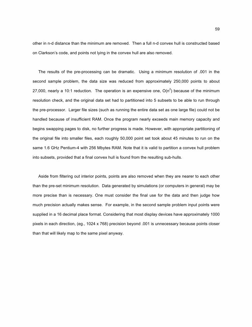
59
other in n-d distance than the minimum are removed. Then a full n-d convex hull is constructed based
on Clarkson’s code, and points not lying in the convex hull are also removed.
The results of the pre-processing can be dramatic. Using a minimum resolution of .001 in the
second sample problem, the data size was reduced from approximately 250,000 points to about
27,000, nearly a 10:1 reduction. The operation is an expensive one, O(n2) because of the minimum
resolution check, and the original data set had to partitioned into 5 subsets to be able to run through
the pre-processor. Larger file sizes (such as running the entire data set as one large file) could not be
handled because of insufficient RAM. Once the program nearly exceeds main memory capacity and
begins swapping pages to disk, no further progress is made. However, with appropriate partitioning of
the original file into smaller files, each roughly 50,000 point set took about 45 minutes to run on the
same 1.6 GHz Pentium-4 with 256 Mbytes RAM. Note that it is valid to partition a convex hull problem
into subsets, provided that a final convex hull is found from the resulting sub-hulls.
Aside from filtering out interior points, points are also removed when they are nearer to each other
than the pre-set minimum resolution. Data generated by simulations (or computers in general) may be
more precise than is necessary. One must consider the final use for the data and then judge how
much precision actually makes sense. For example, in the second sample problem input points were
supplied in a 16 decimal place format. Considering that most display devices have approximately 1000
pixels in each direction, (eg., 1024 x 768) precision beyond .001 is unnecessary because points closer
than that will likely map to the same pixel anyway.
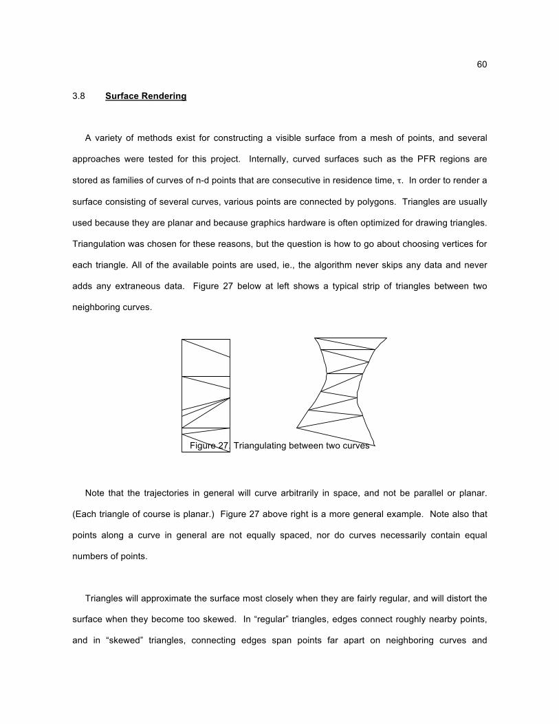
60
3.8 Surface Rendering
A variety of methods exist for constructing a visible surface from a mesh of points, and several
approaches were tested for this project. Internally, curved surfaces such as the PFR regions are
stored as families of curves of n-d points that are consecutive in residence time, ". In order to render a
surface consisting of several curves, various points are connected by polygons. Triangles are usually
used because they are planar and because graphics hardware is often optimized for drawing triangles.
Triangulation was chosen for these reasons, but the question is how to go about choosing vertices for
each triangle. All of the available points are used, ie., the algorithm never skips any data and never
adds any extraneous data. Figure 27 below at left shows a typical strip of triangles between two
neighboring curves.
Figure 27. Triangulating between two curves
Note that the trajectories in general will curve arbitrarily in space, and not be parallel or planar.
(Each triangle of course is planar.) Figure 27 above right is a more general example. Note also that
points along a curve in general are not equally spaced, nor do curves necessarily contain equal
numbers of points.
Triangles will approximate the surface most closely when they are fairly regular, and will distort the
surface when they become too skewed. In “regular” triangles, edges connect roughly nearby points,
and in “skewed” triangles, connecting edges span points far apart on neighboring curves and
61
approach degeneracy as the points approach co-linearity. Figure 28 below, left and right, shows
regular and skewed triangulations, respectively.
Figure 28. Regular and skewed triangles
Both diagrams use the same data points, but notice how the order in which vertices are chosen
affects the quality of the triangles. The right hand diagram results in long, narrow triangles, which will
result in a poor surface. The algorithm used for triangulation is as follows: Consider a set of two
neighboring curves as above. Starting at the same end of both, connect the end points to form the
base of a triangle. Then, consider as possible vertices the next point on either curve. Use a suitable
metric to choose one or the other next point as making a better triangle. Connect the diagonal chord
which crosses between trajectories, to complete the first triangle. This crossing chord becomes the
new base for the next triangle. Repeat the process, always considering as possible vertices the next
unused point in each trajectory, and always choose the “better” one. Finally, at the end, one trajectory
will be completed and the other may still have some unused points at its end. Form a fan of triangles
from the end of the completed trajectory to each unused point in the other.
At each iteration, two candidate points exist, one from each curve, and the question is, what metric
should be used to choose the better triangle. A good metric will keep the resulting triangles well-
behaved, and a poor metric will skew them more and more. Several unsuccessful metrics were
62
attempted, among them minimizing the resulting triangle perimeter, minimizing the ratio of the longest
to shortest side of the resulting triangle, and minimizing the length of the crossing chord.
Best results were achieved by minimizing the difference of path length fractions along the two
trajectories, where the path length fraction is expressed as a fraction of the current path length divided
by the total path length. Intuitively, if one trajectory is 10% complete, then the other should also be
about 10% complete, where the percentage completed is computed using path lengths (not numbers
of data points). Thus, the metric used at each iteration is to choose points that will minimize the
difference between path length fractions, where path length is computed in the 3-d projection space.
(not the full n-d problem space) Recall from Section 2.3.7 that a path or curve is a 1-d parametric
entity, in this case consisting of a set of 3-d points. Triangles are also checked for singularity (collinear
points) by testing for zero cross-product of two sides.
The path length fraction works well in all cases seen so far. The figure below shows examples of
successful and unsuccessful triangulations from the development of the final algorithm.

63
Figure 29. Good and bad triangulations
Skewed triangles from a poor metric
Resulting shading artifacts
Same area well-triangulated
Resulting in improved shading
64
3.9 Lighting
Lighting can add realism and aids understanding, especially for depth perception. 3-d depth
perception is accomplished through 2-d depth cues such as apparent size, perspective convergence,
and shading. Without lighting, each rendered surface has its own self-luminous color, but no shadows
are cast so the color is uniform across the surface. Other depth cues still help in visualizing the
surface, but shading adds a new degree of understandability, albeit at a performance cost. The
application originally began without lighting (self-luminous) to maximize performance, but once lighting
was added, it was clear that the trade-off was well worth it.
Having said that, lighting is a complex topic with a multitude of possibilities, many of which are not
being used here. A simple diffuse white directional light is all that is employed, where the light rays
are all parallel as if the source were infinitely far away. Each surface has a defined diffuse material
color, so that it reflects the same color diffuse light. Diffuse light is reflected in all directions equally, as
opposed to specular light that is reflected in a preferred direction, creating shiny highlights. The light
source maintains its relative direction to the viewpoint, shining downward from the viewpoint at all
times so that surfaces facing normal to the view appear brightest. A slight amount of ambient light is
also added to minimize glare.
A simple lighting model is used not only for performance reasons, but also to avoid distorting or
distracting from the data. Tufte stresses the importance of maintaining data integrity and focus on the
data, as opposed to obscuring data or replacing it with “pretty pictures”. (Tufte, 1983; Tufte, 1990;
Tufte,1997) In keeping with that theme, lighting is used only to help enhance depth perception, but
without features such as specularity that would change surface appearance from the basic colors that
are defined in the data file. Later, if other visible features such as texture or specularity could be used
in a constructive way to represent additional dimensions, then that would justify their use.

65
As a final note, one drawback of using lighting is that shading is created where it may not be
intended. Since surfaces are triangulated, each triangle has a slightly different normal direction than
its neighbors, and light falling on these faces gives the surface a more faceted appearance than when
it was all the same intensity. Hence, the triangular nature of the surface stands out more, even if the
surface should be theoretically smooth. Smooth shading, also known as Gouraud shading, is being
used to interpolate the triangle’s color between the three respective colors of the vertices. (Woo, et al.,
1999) The condition can be further improved by interpolating the normals at each vertex between all of
the triangles that share the vertex, as in Phong shading. (Foley et al., 1997) Presently this is not
done, as all three of the triangle’s vertices have the same normal, that of the triangle’s plane.
66
3.10 Data Probing
Data probing is the opposite of data rendering. Instead of starting with numerical values and
producing a rendered image, probing begins with a rendered image and returns numerical values at
desired places. The method used is to construct a ray extending from the mouse or wand, and
intersect it with all of the visible objects in the current view, as a ray tracer would do. This is done in
the order of points first, then curves, and lastly surfaces.
3.10.1 Probing Points and Curves
The first objects to be checked during probing are the “points of special interest.” These are the
labeled points such as feed point and origin that are identified in the data file. They are relatively few
in number, and are not to be confused with the numerous “ordinary” points that comprise curves.
Finding whether a point lies on a ray is straightforward; the only problem is that chances are that none
of the points lie exactly on the ray. However, the point on the ray which is closest to the given point
can be found (Glassner, 1998) and then the distance of closest approach is computed. This distance
must be less than or equal to some pre-determined probing radius in order to be considered a hit.
One final problem is that the probing radius is a floating-point distance in world coordinates, which
should vary depending on the current view transformation. To be useful, the probing radius should
be equivalent to some small number of pixels in window coordinates (5 pixels,
for example, regardless of the current view). Fortunately, the OpenGL UnProject() command (Woo, et
al., 1999) can be used to compute this probing radius for any view, based on the number of pixels
selected as the margin of probing error. Finally, in case the ray intersects more than one point within
the probe radius, the closest point to the viewer is selected.
Curves are handled similarly. All curves are composed of paths of short lines, and probing the
curves amounts to finding the intersection of a line with the probe ray. Once again, the chances of two
67
lines intersecting exactly in 3-space are small, but from Glassner (Glassner, 1998) one can compute
the respective points of closest approach on the line and the ray, where they are nearest to each
other. Again, “hits” are considered to be locations where the distance of closest approach is within the
probing radius, and from those curves the closest to the viewer is selected.
3.10.2 Probing Surfaces
Since surfaces are rendered as triangles, probing surfaces equates to probing all the visible
triangles. The ray usually intersects more than one triangle, in which case the point of intersection
nearest to the viewer is the result. The n-dimensional concentrations of that point are then displayed.
Finding the point of intersection of a ray and a triangle consists of several sub-steps, which are
outlined in the pseudo-code below (see actual application C++ code, file “probe.cxx” for more details)
a. describe the ray in terms of a parameter t as: ray = base point + t * direction vector
b. construct a plane (ax + by + cz + d = 0) containing the triangle
c. find the point of intersection of the ray with the plane (if it exists) by substituting the ray
equation into the plane equation and solving for t
d. determine if the point of intersection of the ray with the plane actually lies within the interior of
the triangle
The last step, finding whether a point lies within a triangle given that it lies in the triangle’s plane is
actually a sub-problem in itself. Foley and Van Dam (Foley et. al., 1997) give a well-known algorithm
for determining whether a point lies in a general polygon, but here a more specific algorithm for
triangles is used from Glassner. (Glassner, 1998)
Finally, the result of the data probe is a 3-d point in (x,y,z) coordinates that is a projection of the
original n-d data point. The user (eg. chemical engineer) however wants to know the concentrations at
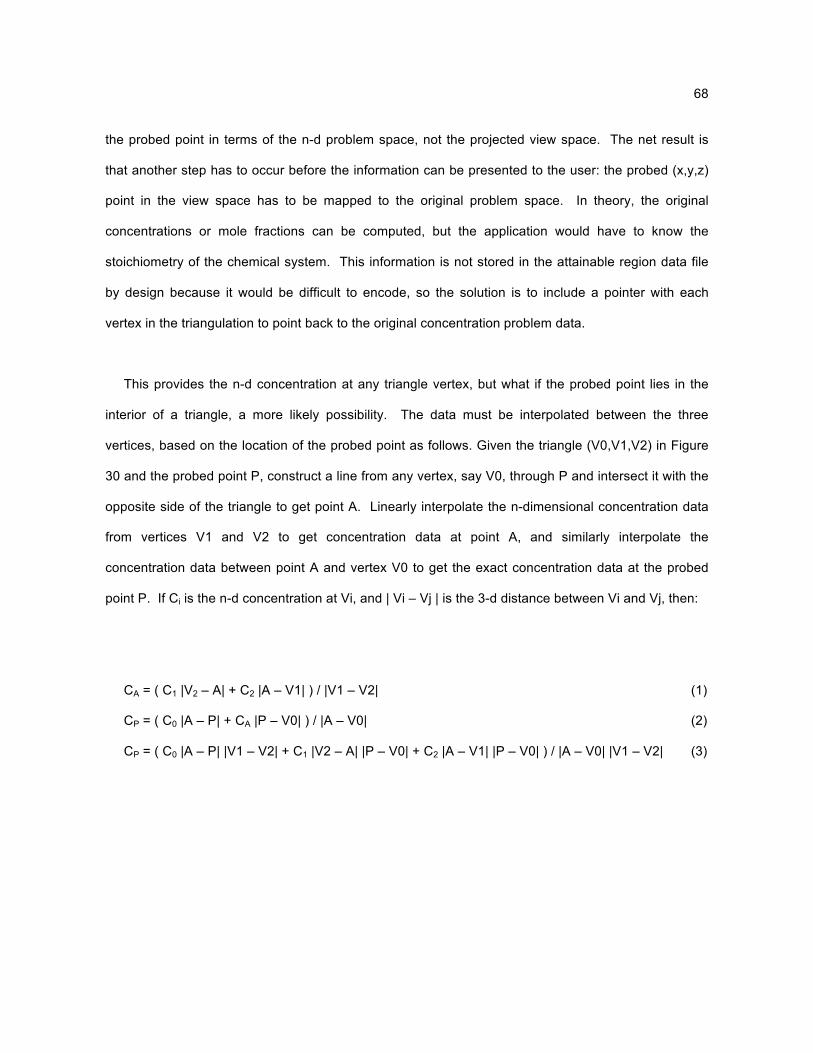
68
the probed point in terms of the n-d problem space, not the projected view space. The net result is
that another step has to occur before the information can be presented to the user: the probed (x,y,z)
point in the view space has to be mapped to the original problem space. In theory, the original
concentrations or mole fractions can be computed, but the application would have to know the
stoichiometry of the chemical system. This information is not stored in the attainable region data file
by design because it would be difficult to encode, so the solution is to include a pointer with each
vertex in the triangulation to point back to the original concentration problem data.
This provides the n-d concentration at any triangle vertex, but what if the probed point lies in the
interior of a triangle, a more likely possibility. The data must be interpolated between the three
vertices, based on the location of the probed point as follows. Given the triangle (V0,V1,V2) in Figure
30 and the probed point P, construct a line from any vertex, say V0, through P and intersect it with the
opposite side of the triangle to get point A. Linearly interpolate the n-dimensional concentration data
from vertices V1 and V2 to get concentration data at point A, and similarly interpolate the
concentration data between point A and vertex V0 to get the exact concentration data at the probed
point P. If Ci is the n-d concentration at Vi, and | Vi – Vj | is the 3-d distance between Vi and Vj, then:
CA = ( C1 |V2 – A| + C2 |A – V1| ) / |V1 – V2| (1)
CP = ( C0 |A – P| + CA |P – V0| ) / |A – V0| (2)
CP = ( C0 |A – P| |V1 – V2| + C1 |V2 – A| |P – V0| + C2 |A – V1| |P – V0| ) / |A – V0| |V1 – V2| (3)
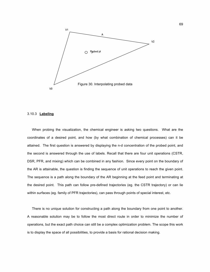
69
Figure 30. Interpolating probed data
3.10.3 Labeling
When probing the visualization, the chemical engineer is asking two questions. What are the
coordinates of a desired point, and how (by what combination of chemical processes) can it be
attained. The first question is answered by displaying the n-d concentration of the probed point, and
the second is answered through the use of labels. Recall that there are four unit operations (CSTR,
DSR, PFR, and mixing) which can be combined in any fashion. Since every point on the boundary of
the AR is attainable, the question is finding the sequence of unit operations to reach the given point.
The sequence is a path along the boundary of the AR beginning at the feed point and terminating at
the desired point. This path can follow pre-defined trajectories (eg. the CSTR trajectory) or can lie
within surfaces (eg. family of PFR trajectories), can pass through points of special interest, etc.
There is no unique solution for constructing a path along the boundary from one point to another.
A reasonable solution may be to follow the most direct route in order to minimize the number of
operations, but the exact path choice can still be a complex optimization problem. The scope this work
is to display the space of all possibilities, to provide a basis for rational decision making.
P
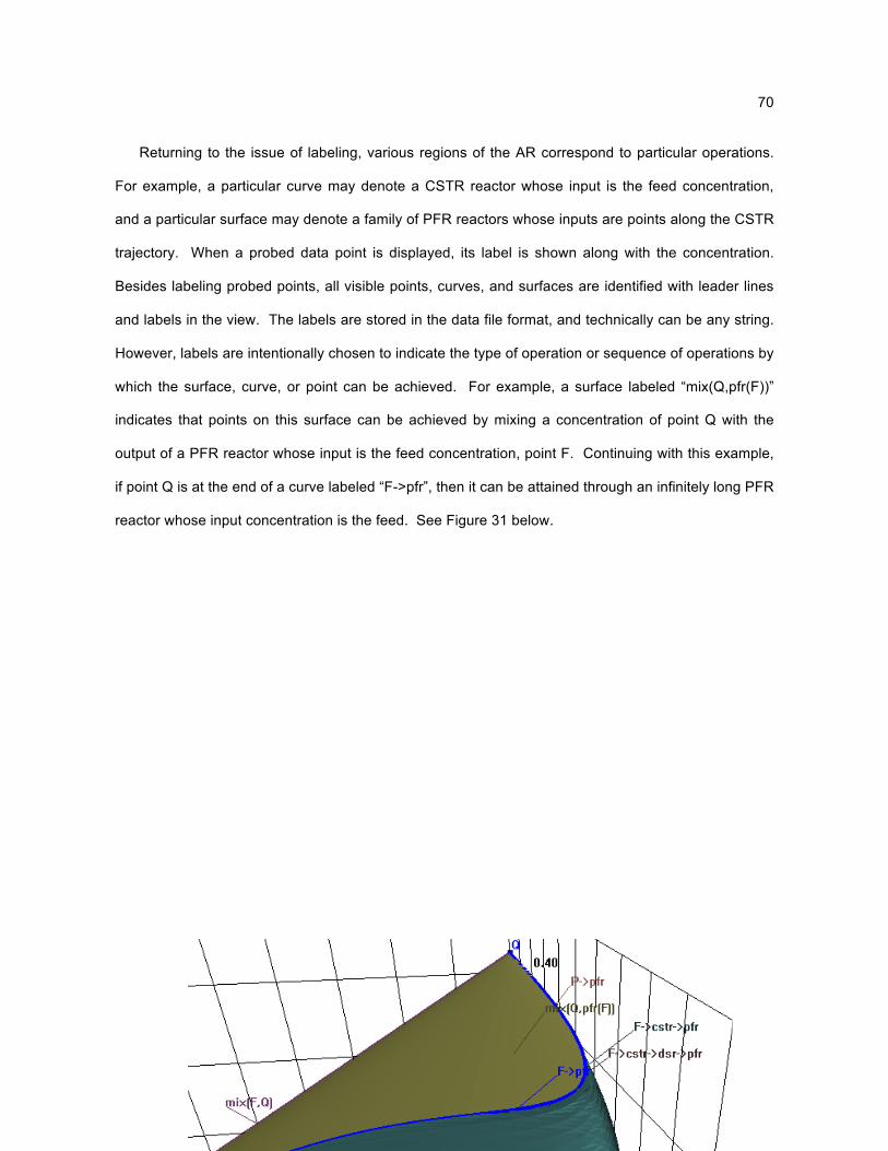
70
Returning to the issue of labeling, various regions of the AR correspond to particular operations.
For example, a particular curve may denote a CSTR reactor whose input is the feed concentration,
and a particular surface may denote a family of PFR reactors whose inputs are points along the CSTR
trajectory. When a probed data point is displayed, its label is shown along with the concentration.
Besides labeling probed points, all visible points, curves, and surfaces are identified with leader lines
and labels in the view. The labels are stored in the data file format, and technically can be any string.
However, labels are intentionally chosen to indicate the type of operation or sequence of operations by
which the surface, curve, or point can be achieved. For example, a surface labeled “mix(Q,pfr(F))”
indicates that points on this surface can be achieved by mixing a concentration of point Q with the
output of a PFR reactor whose input is the feed concentration, point F. Continuing with this example,
if point Q is at the end of a curve labeled “F->pfr”, then it can be attained through an infinitely long PFR
reactor whose input concentration is the feed. See Figure 31 below.

71
Figure 31. Use of labels
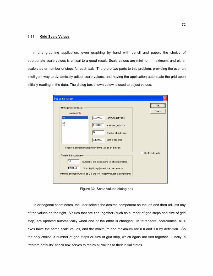
72
3.11 Grid Scale Values
In any graphing application, even graphing by hand with pencil and paper, the choice of
appropriate scale values is critical to a good result. Scale values are minimum, maximum, and either
scale step or number of steps for each axis. There are two parts to this problem: providing the user an
intelligent way to dynamically adjust scale values, and having the application auto-scale the grid upon
initially reading in the data. The dialog box shown below is used to adjust values:
Figure 32. Scale values dialog box
In orthogonal coordinates, the user selects the desired component on the left and then adjusts any
of the values on the right. Values that are tied together (such as number of grid steps and size of grid
step) are updated automatically when one or the other is changed. In tetrahedral coordinates, all 4
axes have the same scale values, and the minimum and maximum are 0.0 and 1.0 by definition. So
the only choice is number of grid steps or size of grid step, which again are tied together. Finally, a
“restore defaults” check box serves to return all values to their initial states.
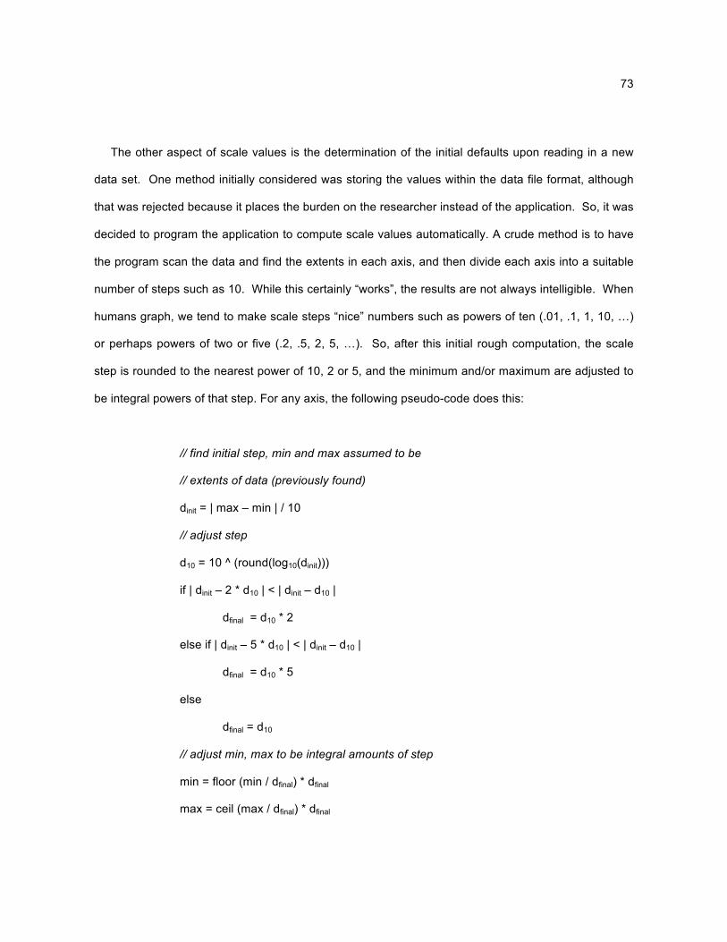
73
The other aspect of scale values is the determination of the initial defaults upon reading in a new
data set. One method initially considered was storing the values within the data file format, although
that was rejected because it places the burden on the researcher instead of the application. So, it was
decided to program the application to compute scale values automatically. A crude method is to have
the program scan the data and find the extents in each axis, and then divide each axis into a suitable
number of steps such as 10. While this certainly “works”, the results are not always intelligible. When
humans graph, we tend to make scale steps “nice” numbers such as powers of ten (.01, .1, 1, 10, …)
or perhaps powers of two or five (.2, .5, 2, 5, …). So, after this initial rough computation, the scale
step is rounded to the nearest power of 10, 2 or 5, and the minimum and/or maximum are adjusted to
be integral powers of that step. For any axis, the following pseudo-code does this:
// find initial step, min and max assumed to be
// extents of data (previously found)
dinit = | max – min | / 10
// adjust step
d10 = 10 ^ (round(log10(dinit)))
if | dinit – 2 * d10 | < | dinit – d10 |
dfinal = d10 * 2
else if | dinit – 5 * d10 | < | dinit – d10 |
dfinal = d10 * 5
else
dfinal = d10
// adjust min, max to be integral amounts of step
min = floor (min / dfinal) * dfinal
max = ceil (max / dfinal) * dfinal
74
4. SAMPLE PROBLEM 1
The first sample problem around which the application was initially designed is a classic in AR
literature. J.G. van de Vusse first published this problem in 1964, (van de Vusse, 1964) and the
version used here is taken from Feinberg and Hildebrandt. (Feinberg and Hildebrandt, 1997) The
chemical system is defined by the following equations.
4.1 Equations and Rate Laws
Chemical equations:
A1 ! A2 k1 = 1 [s-1]
A2 ! A4 k2 = 1 [s-1]
2A1 ! A3 k3 = 10 [m3 / (mol s)]
Let ci be the concentration of Ai
Feed point: c1 = 1.0, c2 = c3 = c4 = 0.0
Rate laws:
rA1 = -r1 – 2r3 = -k1c1 –2 k3c12 = -c1 – 20c1
2 [mol / (m3 s)] (1)
rA2 = r1 - r2 = k1c1 – k2c2 = c1 – c2 (2)
rA3 = r3 = k3c12 = 10 c1
2 (3)
rA4 = r2 = k2c2 = c2 (4)
Through a combination of computations and assistance from a differential equation solver known
as Polymath, (Cutlip, 2003) data points were generated for a CSTR trajectory, DSR trajectory, PFR
trajectories, and mixing regions. The details of those derivations appear in Appendix D.
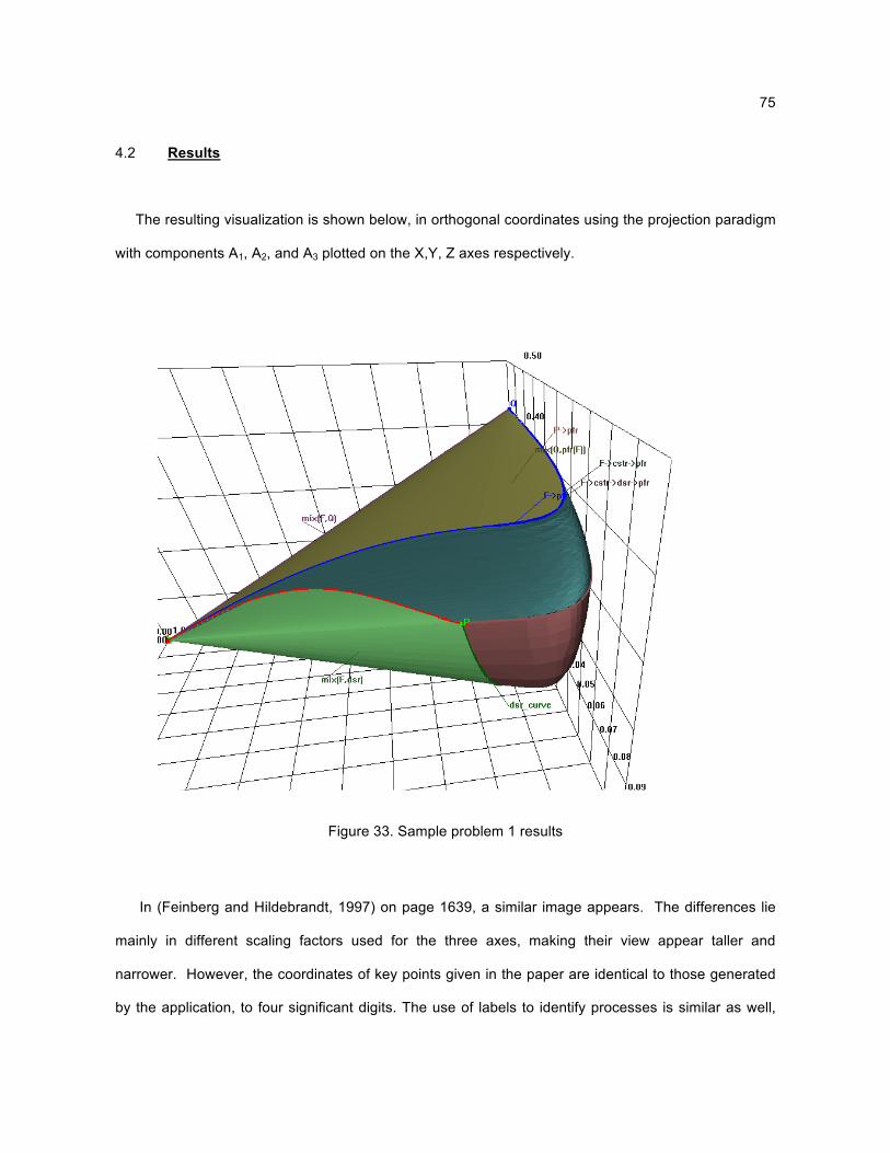
75
4.2 Results
The resulting visualization is shown below, in orthogonal coordinates using the projection paradigm
with components A1, A2, and A3 plotted on the X,Y, Z axes respectively.
Figure 33. Sample problem 1 results
In (Feinberg and Hildebrandt, 1997) on page 1639, a similar image appears. The differences lie
mainly in different scaling factors used for the three axes, making their view appear taller and
narrower. However, the coordinates of key points given in the paper are identical to those generated
by the application, to four significant digits. The use of labels to identify processes is similar as well,
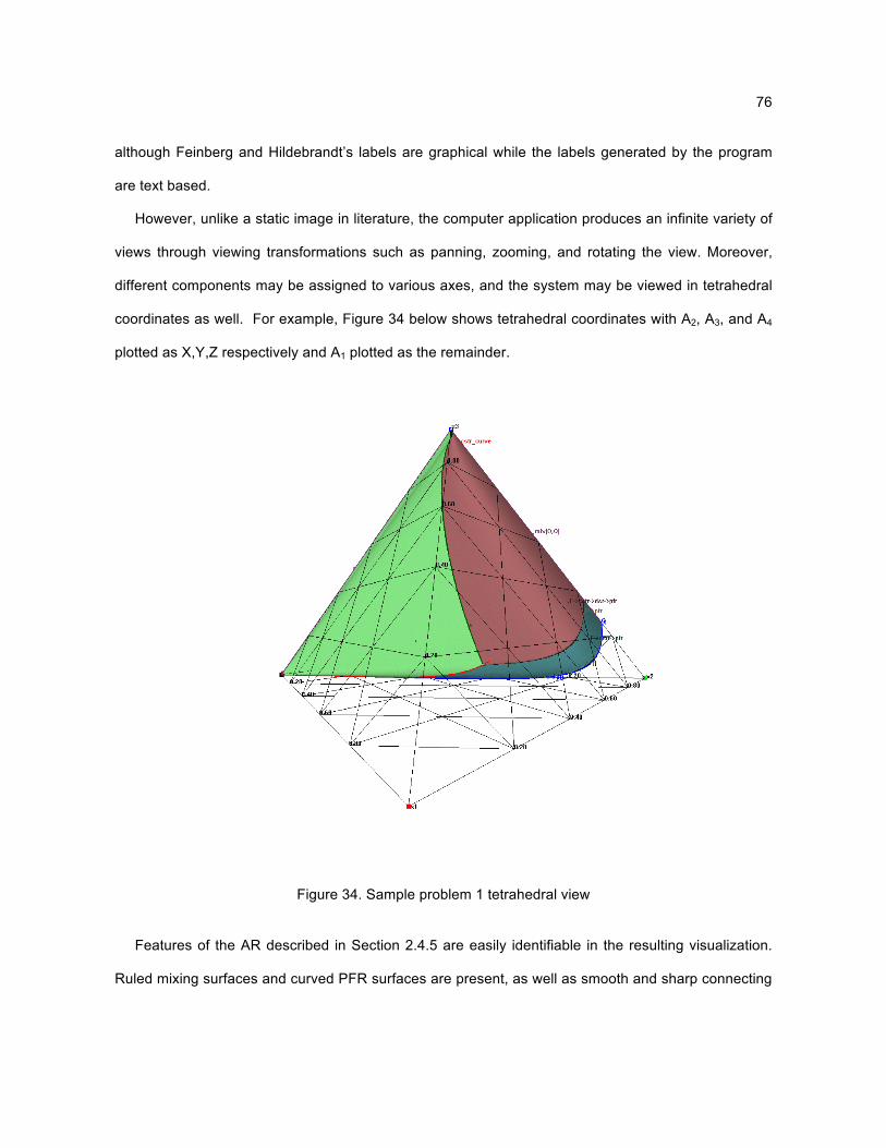
76
although Feinberg and Hildebrandt’s labels are graphical while the labels generated by the program
are text based.
However, unlike a static image in literature, the computer application produces an infinite variety of
views through viewing transformations such as panning, zooming, and rotating the view. Moreover,
different components may be assigned to various axes, and the system may be viewed in tetrahedral
coordinates as well. For example, Figure 34 below shows tetrahedral coordinates with A2, A3, and A4
plotted as X,Y,Z respectively and A1 plotted as the remainder.
Figure 34. Sample problem 1 tetrahedral view
Features of the AR described in Section 2.4.5 are easily identifiable in the resulting visualization.
Ruled mixing surfaces and curved PFR surfaces are present, as well as smooth and sharp connecting
77
curves. It is instructive to refer back to that section while running the application and note the
correspondence between AR theory and practical results.
The van de Vusse problem served as a foundation around which the “core” of the application was
developed. Through this problem, many program features were developed and tested, including n-d
architecture, dimension reduction, tetrahedral coordinates, standard file format, data probing,
interactive viewing, and the user interface. It is a classic AR problem, and the fact the results
generated by the application matched other published results was encouraging. The envelope of AR
visualization was extended through some of the aforementioned features, but van de Vusse has been
visualized many times before using other methods, albeit at the cost of discarding at least one
variable. Even our collaborators have such a visualization in Appendix B, generated using MATLAB
(MATLAB, 2003). A second, more demanding example was required.
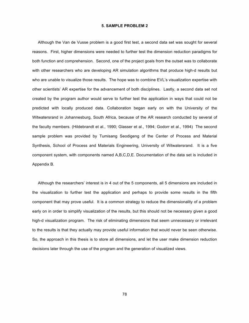
78
5. SAMPLE PROBLEM 2
Although the Van de Vusse problem is a good first test, a second data set was sought for several
reasons. First, higher dimensions were needed to further test the dimension reduction paradigms for
both function and comprehension. Second, one of the project goals from the outset was to collaborate
with other researchers who are developing AR simulation algorithms that produce high-d results but
who are unable to visualize those results. The hope was to combine EVL’s visualization expertise with
other scientists’ AR expertise for the advancement of both disciplines. Lastly, a second data set not
created by the program author would serve to further test the application in ways that could not be
predicted with locally produced data. Collaboration began early on with the University of the
Witwatersrand in Johannesburg, South Africa, because of the AR research conducted by several of
the faculty members. (Hildebrandt et al., 1990; Glasser et al., 1994; Godorr et al., 1994) The second
sample problem was provided by Tumisang Seodigeng of the Center of Process and Material
Synthesis, School of Process and Materials Engineering, University of Witwatersrand. It is a five
component system, with components named A,B,C,D,E. Documentation of the data set is included in
Appendix B.
Although the researchers’ interest is in 4 out of the 5 components, all 5 dimensions are included in
the visualization to further test the application and perhaps to provide some results in the fifth
component that may prove useful. It is a common strategy to reduce the dimensionality of a problem
early on in order to simplify visualization of the results, but this should not be necessary given a good
high-d visualization program. The risk of eliminating dimensions that seem unnecessary or irrelevant
to the results is that they actually may provide useful information that would never be seen otherwise.
So, the approach in this thesis is to store all dimensions, and let the user make dimension reduction
decisions later through the use of the program and the generation of visualized views.
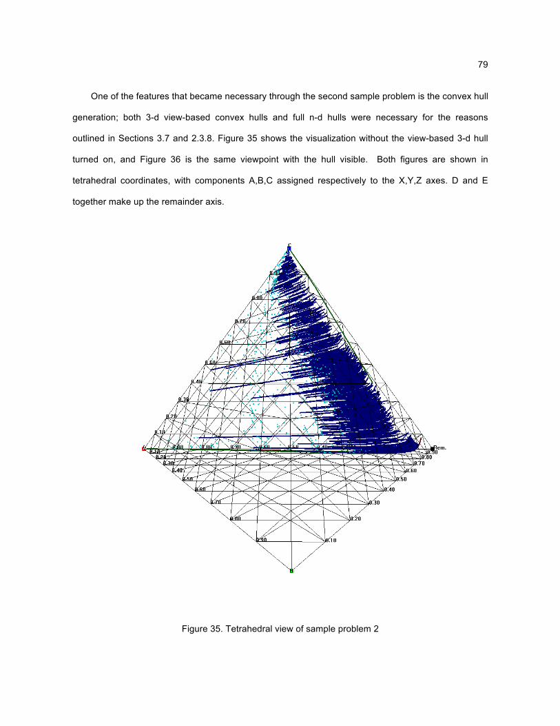
79
One of the features that became necessary through the second sample problem is the convex hull
generation; both 3-d view-based convex hulls and full n-d hulls were necessary for the reasons
outlined in Sections 3.7 and 2.3.8. Figure 35 shows the visualization without the view-based 3-d hull
turned on, and Figure 36 is the same viewpoint with the hull visible. Both figures are shown in
tetrahedral coordinates, with components A,B,C assigned respectively to the X,Y,Z axes. D and E
together make up the remainder axis.
Figure 35. Tetrahedral view of sample problem 2
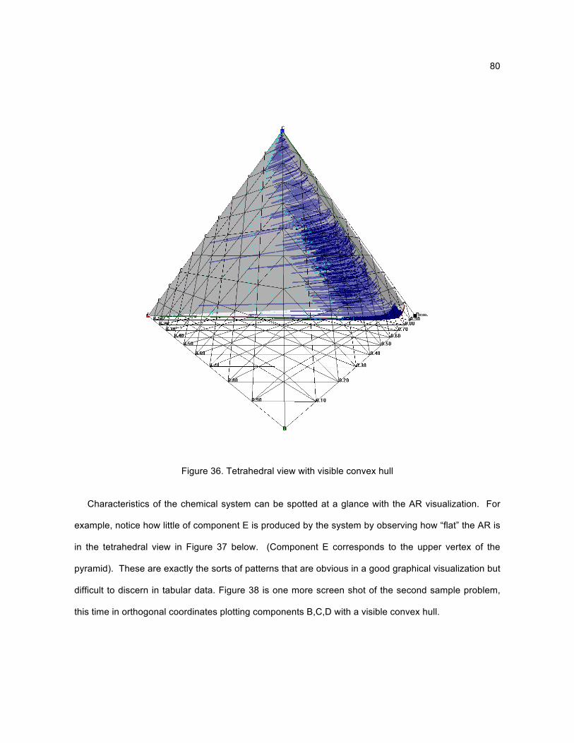
80
Figure 36. Tetrahedral view with visible convex hull
Characteristics of the chemical system can be spotted at a glance with the AR visualization. For
example, notice how little of component E is produced by the system by observing how “flat” the AR is
in the tetrahedral view in Figure 37 below. (Component E corresponds to the upper vertex of the
pyramid). These are exactly the sorts of patterns that are obvious in a good graphical visualization but
difficult to discern in tabular data. Figure 38 is one more screen shot of the second sample problem,
this time in orthogonal coordinates plotting components B,C,D with a visible convex hull.
81
Figure 37. Tetrahedral view with trace amounts of component E
Figure 38. Orthogonal view of B,C,D
This second problem further enhanced current AR visualization techniques with the addition of n-d
and 3-d convex hulls. It also provided more opportunity for collaboration and testing of the application
by other parties. The features developed for the first sample problem together with those added for the
second combine to make the application a useful tool for the visualization of high-d ARs. Compared to
the survey of visualizations in Section 2.4.6, the ability to view a 5-d problem in 5-d space is a
significant step in AR visualization. Our collaborators had no way to previously view these results.

82
Feedback from Tumisang Seodigeng of the University of Witwatersrand has been positive. The
following excerpts are from personal communications via e-mail after sharing results and the program:
“Thank you for the program and notes. The first set was very fascinating, I like the idea of switching
from one 3D projection to the other with ease (say ABD to ABE) … I have looked at the package Tom
sent me some time ago. It was impressive; he managed to sort out the data separation problem.”
(Seodigeng, 2003, personal communication) The data separation problem Seodigeng refers to is the
fact that points produced by his simulation were disorganized and thus could not be used to render
surfaces using triangulation methods, ie., could not be separated into adjacent curves. This was a
driving force for inclusion of convex hulls in the application.
One final distinction between the second and first sample problems is data size. The van de Vusse
example consisted of roughly 5000 data points, while the second problem consisted of around
270,000 points. This was another factor that necessitated the use of an n-d convex hull in order to
pre-process the data set and reduce its size to around 25,000 points, a size that could be viewed
interactively on current computer hardware. As ARs grow to higher dimensions and file sizes and data
set sizes increase, the techniques developed here can be used to make large data more manageable.
83
6. CONCLUSION
Background research having been conducted, concepts have been applied to develop a working
interactive visualization tool capable of viewing n-d ARs. The application has been tested through two
sample problems, and results have been shared with collaborators. This chapter summarizes
knowledge gained and plans for future work.
6.1 Summary
Engineering problems that rely on graphical solutions work well in small numbers of dimensions
such as 2 or 3, but are difficult to visualize when the dimensional space becomes large. However,
scientific and engineering actual problems are multi-dimensional by nature, and graphical
visualizations are desired because they leverage the visual perception of the human mind to quickly
see patterns and draw conclusions about the data.
One such graphical method in the domain of chemical reactor design synthesis is the attainable
region, or AR. The AR is a closed volume in n-d space that represents all possible chemical
compositions that can be attained from a chemical system, given some starting feed composition.
After research of chemical reactor design synthesis and a thorough survey of AR literature, principles
of computer science and scientific visualization were combined to produce a working computer
application capable of visualizing n-d ARs. The application program is capable of reading AR data
files of the format “.ard” in general numbers of dimensions, and producing views through dimension
reduction. Two choices of coordinate systems are available, orthogonal and tetrahedral, along with the
capability to view selected combinations of three or four components at a time. A 3-d convex hull
feature is included for checking the AR for convexity and for viewing non-ordered surfaces, and n-d
convex hulls are also utilized in a pre-processing filtering utility program. Other aspects of the
application include data probing, interactive view transformations, grid scale adjustment, color choices,
and a functional user interface including a comprehensive help system.
84
Two sample problems were used to test the application and develop it further. The first problem,
the 4-d van de Vusse system is a classic in AR literature. After successfully completing this, a more
difficult second test problem was sought. From the outset, one of the goals of this work has also been
to collaborate with researchers in the field, because they are the real AR experts. A partnership was
formed with the University of Witwatersrand, South Africa, and a second 5-d data set from research
currently being conducted was tested. The data was more demanding than the first problem, and
forced several new features to be included in the application program. Successful visualizations were
shared with the researchers, along with a copy of the application itself. Communication continues
between the research parties, and the collaborative effort has benefited all involved. Preliminary
feedback from collaborators has been positive. Moreover, a personal visit from Mr. Seodigeng to UIC
and EVL is expected later this year, where we expect to meet for the first time in person and discuss
findings and future work. The AR collaboration and visualization is expected to continue well beyond
the completion of the master’s thesis. On a personal note, the opportunity to aid other researchers in
their work and the ability to contribute to scientific research in a tangible way has been personally very
rewarding.
6.2 Accomplishments
The main accomplishments of this thesis can be grouped into two categories: major contributions
and other accomplishments. Major contributions enhance the current state of AR visualization. Other
accomplishments perhaps do not extend existing work in and of themselves, but were necessary in
order to achieve the major contributions and are worthwhile items of knowledge gained. The table
below summarizes these categories.
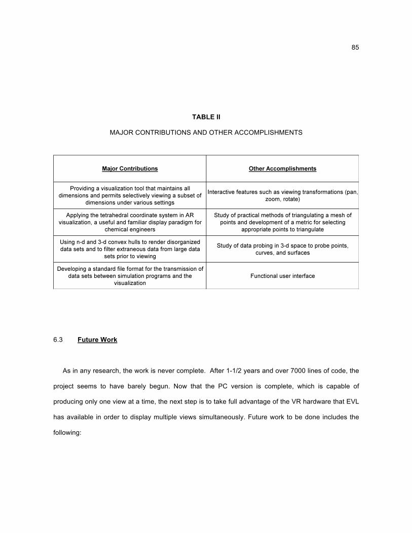
85
TABLE II
MAJOR CONTRIBUTIONS AND OTHER ACCOMPLISHMENTS
6.3 Future Work
As in any research, the work is never complete. After 1-1/2 years and over 7000 lines of code, the
project seems to have barely begun. Now that the PC version is complete, which is capable of
producing only one view at a time, the next step is to take full advantage of the VR hardware that EVL
has available in order to display multiple views simultaneously. Future work to be done includes the
following:
86
• Completing the sectioning paradigm of dimension reduction
• Porting the application to another medium such as a tiled display (Perspectile) or auto-stereo tiled
display (Varrier)
• Including simultaneous display of multiple views (appropriate for a tiled display)
• Allowing any combination of components to be displayed on any axis, similar to the function of the
tetrahedral remainder axis in the present implementation
• Completing the analysis of convexity properties during projection in the orthogonal and tetrahedral
coordinate systems
• Continuing collaboration with researchers to further evaluate the application and determine further
needs
87
CITED LITERATURE
Abbott, E.A.: Flatland A Romance of Many Dimensions. Mineola NY, Dover Publications, 1952. Achenie, L.E.K., Biegler, L.T.: Algorithmic Synthesis of Chemical Reactor Networks Using
Mathematical Programming. Industrial and Engineering Chemistry Research 25 no. 4: 621-627, 1986.
Balakrishna, S., Biegler, L.T.: Constructive Targeting Approaches for the Synthesis of Chemical
Reactor Networks. Industrial and Engineering Chemistry Research 31 no. 1: 300-312, 1992. Bell, J.T.: A Computational Representation of Thermodynamic Surfaces for Use in Process Flowsheet
Calculations. Master’s thesis, University of Wisconsin – Madison, Madison, WI, 1987. Clarkson K.L.: A Program for Convex Hulls. http://cm.bell-labs.com/netlib/voronoi/hull.html, 2003. Clarkson, K.L., Mehlhorn, K., Seidel, R.: Four Results on Randomized Incremental Constructions.
Comp. Geom.: Theory and Applications 185-121, 1993. Cruz-Neira, C.,Sandin, D., DeFanti, T.: Surround-Screen Projection-Based Virtual Reality: The Design
and Implementation of the CAVE. Computer Graphics, ACM SIGGRAPH 135-142, 1993. Cutlip, M.: Polymath Software. http://www.polymath-software.com, 2003. EVL: www.evl.uic.edu, 2003. Feinberg, M.: Optimal Reactor Design From a Geometric Viewpoint. Part II. Critical Sidestream
Reactors. Chemical Engineering Science 55: 2455-2479, 2000. Feinberg, M., Hildebrandt, D.: Optimal Reactor Design from a Geometric Viewpoint - I. Universal
Properties of the Attainable Region. Chemical Engineering Science 52 no. 10: 1637-1665, 1997.
Fogler, H. Scott.: Elements of Chemical Reaction Engineering 3rd Edition. Englewood Cliffs, NJ,
Prentice Hall, 1999. Foley, James D., Van Dam, Andries, Feiner, Steven K., Hughes, John F.: Computer Graphics
Principles and Practice 2nd Edition. Reading, MA, Addison Wesley, 1997. Glasser, D., Hildebrandt, D., Crowe, C.: A Geometric Approach to Steady Flow Reactors: The
Attainable Region and Optimization in Concentration Space. Industrial and Engineering Chemistry Research 26 no. 9: 1803-1810, 1987.
Glasser, B.J., Hildebrandt D., Glasser D.: Optimal Mixing for Exothermic Reversible Reactions.
Industrial and Engineering Chemistry Research 31 no. 6: 1541-1549, 1992. Glasser, D. Hildebrandt, D., Godorr, S.: The Attainable Region for Segregated, Maximum, Mixed, and
Other Reactor Models. Industrial and Engineering Chemistry Research 33 no. 5: 1136-1144, 1994.
Glassner, Andrew S.: Graphics Gems. San Diego, Academic Press, 1998. Godorr, S., Hildebrandt, D., Glasser, D.: The Attainable Region for Systems with Mixing and Multiple-
Rate Processes: Finding Optimal Reactor Structures. Chemical Engineering Journal 54: 175-186, 1994.
88
Goldberg, A.: Smalltalk-80: The Interactive Programming Environment. Reading, MA, Addison-
Wesley, 1984. Hildebrandt, D., Glasser, D., Crowe, C.: Geometry of the Attainable Region Generated by Reaction
and Mixing: With and Without Constraints. Industrial and Engineering Chemistry Research 29 no. 1: 49-58, 1990.
Horn, F.: Attainable and Non-Attainable Regions in Chemical Reaction Technique. Third European
Symposium on Chemical Reaction Engineering New York, Pergamon Press, 1964. Johnson, A.: User Interface Design and Programming. http://www.evl.uic.edu/aej/422/index.html,
2002 JuxtaView: http://www.evl.uic.edu/art/template_art_project.php3?indi=242, 2002 Kauchali, S., Rooney, W.C., Biegler, L.T.: Glasser, D. Hildebrandt, D. Linear Programming
Formulations for Attainable Region Analysis. Chemical Engineering Science 57: 2015-2028, 2002.
Lakshmanan, A., Biegler, L.T.: Synthesis of Optimal Chemical Reactor Networks. Industrial and
Engineering Chemistry Research 35 no. 4: 1344-1353, 1996. Lambert: Convex Hull Algorithms. http://www.cse.unsw.edu.au/~lambert/java/3d/hull.html, 1998. MATLAB: www.mathworks.com, 2003. Murty, Katta G.: Linear Programming. New York, John Wiley & Sons, 1983. Nielson, G., Hagen, H., Muller, H.: Scientific Visualization. IEEE Computer Society Press, 1997. Nisoli, A., Malone, M. F., Doherty, M. F.: Attainable Regions for Reaction with Separation. AIChe
Journal 43 no. 2: 374-387, 1997. Norman, D.: The Design of Everyday Things. New York, Doubleday, 1988. Renambot, L., van der Schaaf, T.: Enabling Tiled Displays for Education.
http://www.cs.vu.nl/~renambot/vr/papers/ccviz02.pdf, 2003. Sandin, D., Margolis, T., Dawe, G., Leigh, J., DeFanti, T.: The Varrier Auto-Stereographic Display.
SPIE 4297 no. 25: 2001. Schneiderman, B.: Designing the User Interface (3rd edition). Reading, MA, Addison Wesley Longman. Sherman, W., Craig, A.: Understanding Virtual Reality. San Francisco, Morgan Kaufmann Publishers,
2003. Smith, R. L., Malone, M. F.: Attainable Regions for Polymerization Reaction Systems. Industrial and
Engineering Chemistry Research 36 no. 4: 1076-1084, 1997. Thomas, G.B. Jr.,Finney, R.L.: Calculus and Analytic Geometry. Reading, MA, Addison-Wesley, 1981.

89
Tufte, E. R.: The Visual Display of Quantitative Information. Cheshire, Connecticut, Graphics Press, 1983.
Tufte, E. R.: Envisioning Information. Cheshire, Connecticut, Graphics Press, 1990. Tufte, E. R.: Visual Explanations. Cheshire, Connecticut, Graphics Press, 1997. van de Vusse, J.G.: Plug-Flow Type Reactor vs. Tank Reactor. Chemical Engineering Science 19:
994-997, 1964. Weiss, M. A.: Data Structures & Algorithm Analysis in C++, 2nd Edition. Reading, MA, Addison Wesley
Longman, 1999. Woo, M., Neider, J., Davis, T., Shreiner, D.: OpenGL Programming Guide. Reading, MA, Addison
Wesley Longman, 1999.
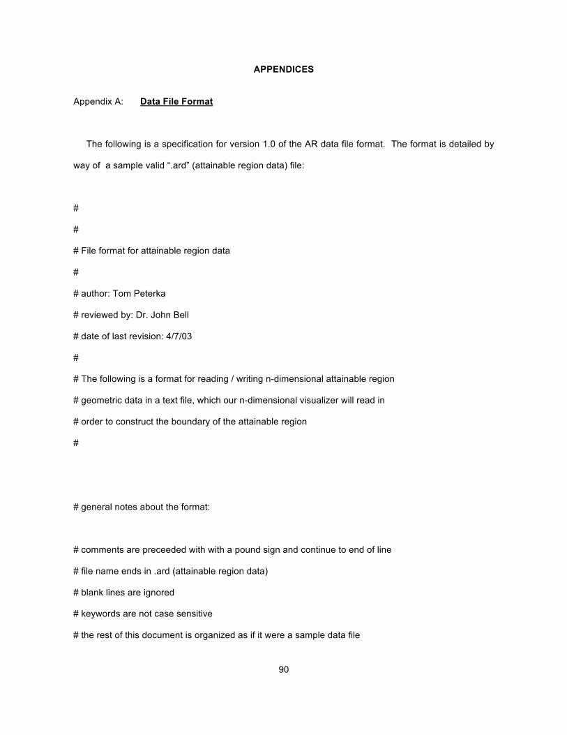
90
APPENDICES
Appendix A: Data File Format
The following is a specification for version 1.0 of the AR data file format. The format is detailed by
way of a sample valid “.ard” (attainable region data) file:
#
#
# File format for attainable region data
#
# author: Tom Peterka
# reviewed by: Dr. John Bell
# date of last revision: 4/7/03
#
# The following is a format for reading / writing n-dimensional attainable region
# geometric data in a text file, which our n-dimensional visualizer will read in
# order to construct the boundary of the attainable region
#
# general notes about the format:
# comments are preceeded with with a pound sign and continue to end of line
# file name ends in .ard (attainable region data)
# blank lines are ignored
# keywords are not case sensitive
# the rest of this document is organized as if it were a sample data file
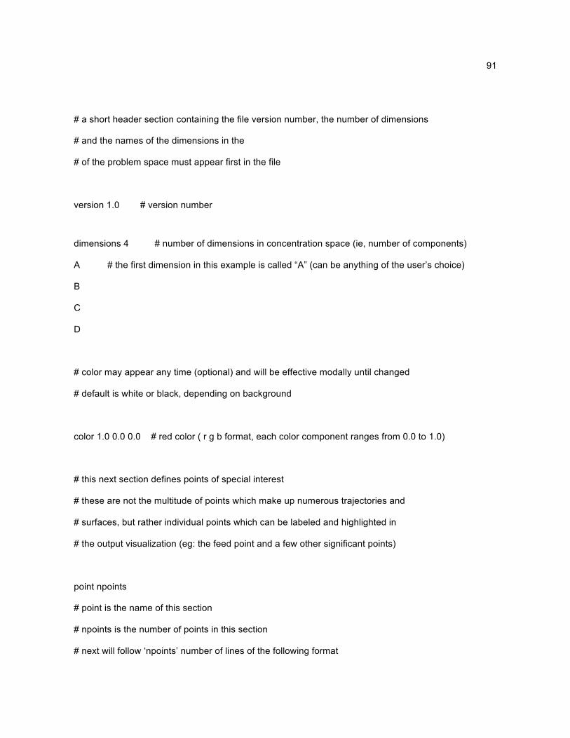
91
# a short header section containing the file version number, the number of dimensions
# and the names of the dimensions in the
# of the problem space must appear first in the file
version 1.0 # version number
dimensions 4 # number of dimensions in concentration space (ie, number of components)
A # the first dimension in this example is called “A” (can be anything of the user’s choice)
B
C
D
# color may appear any time (optional) and will be effective modally until changed
# default is white or black, depending on background
color 1.0 0.0 0.0 # red color ( r g b format, each color component ranges from 0.0 to 1.0)
# this next section defines points of special interest
# these are not the multitude of points which make up numerous trajectories and
# surfaces, but rather individual points which can be labeled and highlighted in
# the output visualization (eg: the feed point and a few other significant points)
point npoints
# point is the name of this section
# npoints is the number of points in this section
# next will follow ‘npoints’ number of lines of the following format
92
a b c d [T/F] [label]
# a b c d are the component concentrations, replace with floating point numbers or scientific notation
# label is optional, and will be displayed next to the point
# [T / F] is a visibility flag, T = draw the object, F= don't draw
# visibility is optional, except when a label is used, visibility is
# mandatory (to enable parsing)
color 0.0 1.0 0.0 # switching to blue color, for example
a b c d [T/F] [label] # labels may have spaces, and extend to the end of line
a b c d # default visibility is T, no label for this object
...
# this next section defines curves
# curves are used in a general sense to include: a individual point, a line segment
# (2 points), or a trajectory (any number of points)
# curves may be of the following types: mixing line segment, CSTR trajectory,
# DSR trajectory, or PFR trajectory
# note that any of the above curve types may be degenerate and have only one point
mix npoints [T/F] [label] # mixing line segment, 1 <= npoints <= 2
a b c d
a b c d
mix npoints [T/F] [label] # each curve individually identified by a new command
a b c d
93
a b c d
cstr npoints [T/F] [label] # CSTR trajectory, npoints >= 1
a b c d
...
dsr npoints [T/F] [label] # DSR trajectory, npoints >= 1
a b c d
...
pfr npoints [T/F] [label] # PFR trajctory, npoints >= 1
a b c d
# visibility is used in the same way as above in the point section
# label is similar, except that labels are required whenever the curve will be referred to below in a
surface
# this is typical, so most of the curves will have labels, and these labels are not displayed in the
visualization
...
# this last section defines surfaces
# surfaces are a triangulation of 2 or more of the above curve types
# if the number of curves is > 2, then the curves must all be of the same type
# if ncurves = 2, then the curve types may the same or different
# if different, then the result is a mixing surface between the 2 curves
# if ncurves > 2, then the curves must be listed in order (adjacent in the surface)
# ie, the surface will be triangulated by taking two adjacent curves at a time

94
surface ncurves [T/F] [label]
label 1 # label of a curve
label 2 # label of a curve
...
# default color for surfaces is the average of constituent curve colors
# (specific color can always be given with the color command (recommended))
95
Appendix B: Sample Problem 2 Materials
The following two documents were provided by Tumisang Seodigeng. They are re-printed here for
reference as supporting documents for the second sample problem, without any corrections or
modification. The entire documents are included, including any fonts, figures, etc. that appeared.
Figures are not listed in the table of figures and fonts may not be the same as in the thesis text. No
attempts were made to modify any of this data; it is meant to be included as a whole, in its original
form. The documents were received as personal communication, not as published or copyrighted
material.
B.1 Initial Documentation of Sample Problem 2 Dataset
The following is an initial document that accompanied the data set (TP)
The 4D study case
A k1f !k2r B k3"C
!k4 k5f"k6r
#D E
We are looking at the ABDE space. We built the candidate ARs using the algorithm we call ‘DSR Algorithm’.
The DSR algorithm traces out the optimal DSR (Feinberg 2000 a and b) using constant alpha values. We believe that a DSR in
4D is a surface, (as it is a curve in 3D).
My algorithm constructs 3D ARs successfully. These are the results for a 4D trial. I am working in the ABDE space.
The attached files are
cstr.txt contains cstr loci from feed. Columns are [ A B C D E tau]
96
pfr.txt plug flow trajectory from feed. Columns are [ A B C D E tau]
cdsrxtr.txt points on the DSR surface, Columns are [ A B C D E tau alpha]
pfrhiways.txt manifolds of pfr trajectories starting from the DSR surface
Columns are [ A B C D E tau alpha]
Space.txt all points in the space, (mess!)
Tau – residence time
Alpha – mixing policy value
If negative the point is a CSTR
Zero for a pfr
Any positive value for a DSR
There is also a cdsrxtr.mat file attached which as matlab file containing binary data of the above. Abde4d points on the DSR
surface. Others have the same name as above.
Extras are
k - rate constants as in the reaction above
alpha – constant alpha grid
co – feed
B.2 Follow-Up Document
Later, a document was received from Mr. Seodigeng clarifying the determination of the alpha policy
used in DSR tractories. Recall that alpha refers to the sidestream mixing policy for a differential
sidestream reactor, or DSR. This document is re-printed below. Again, it was received as personal
communication, not as published copyrighted material. No changes, corrections, or additions were
made to it. (TP)
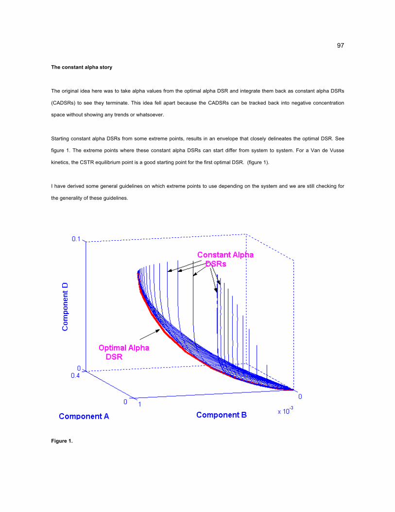
97
The constant alpha story
The original idea here was to take alpha values from the optimal alpha DSR and integrate them back as constant alpha DSRs
(CADSRs) to see they terminate. This idea fell apart because the CADSRs can be tracked back into negative concentration
space without showing any trends or whatsoever.
Starting constant alpha DSRs from some extreme points, results in an envelope that closely delineates the optimal DSR. See
figure 1. The extreme points where these constant alpha DSRs can start differ from system to system. For a Van de Vusse
kinetics, the CSTR equilibrium point is a good starting point for the first optimal DSR. (figure 1).
I have derived some general guidelines on which extreme points to use depending on the system and we are still checking for
the generality of these guidelines.
Figure 1.
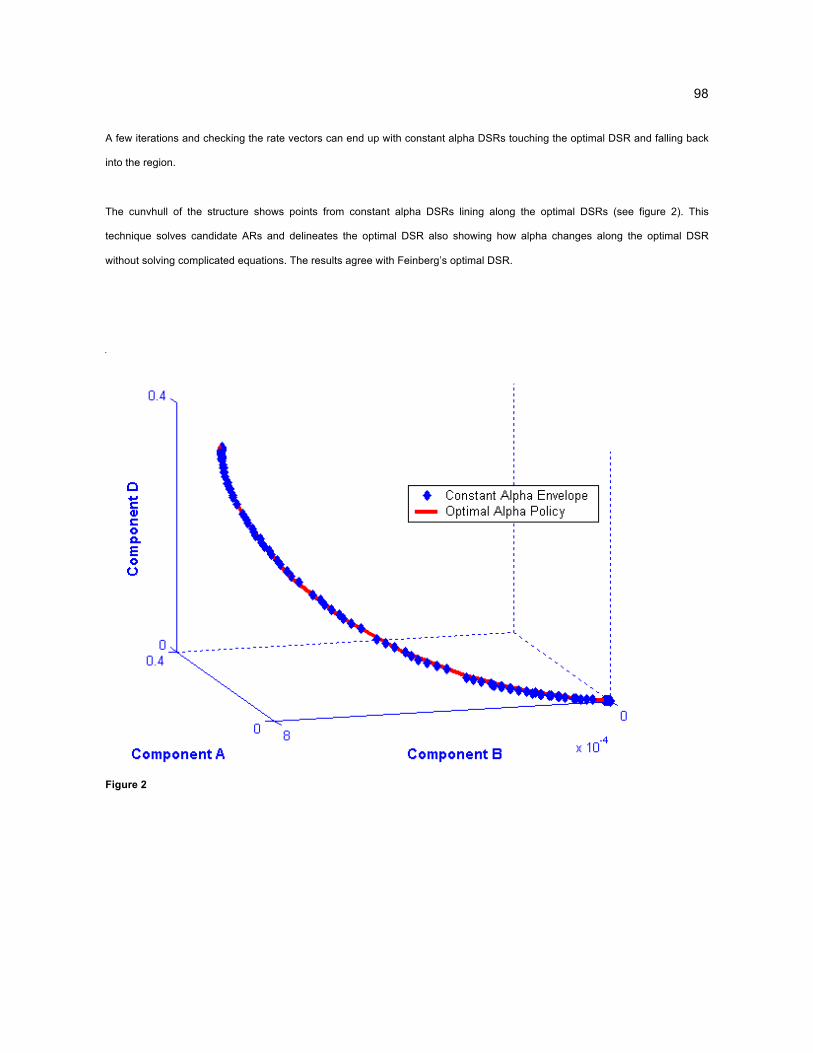
98
A few iterations and checking the rate vectors can end up with constant alpha DSRs touching the optimal DSR and falling back
into the region.
The cunvhull of the structure shows points from constant alpha DSRs lining along the optimal DSRs (see figure 2). This
technique solves candidate ARs and delineates the optimal DSR also showing how alpha changes along the optimal DSR
without solving complicated equations. The results agree with Feinberg’s optimal DSR.
Figure 2
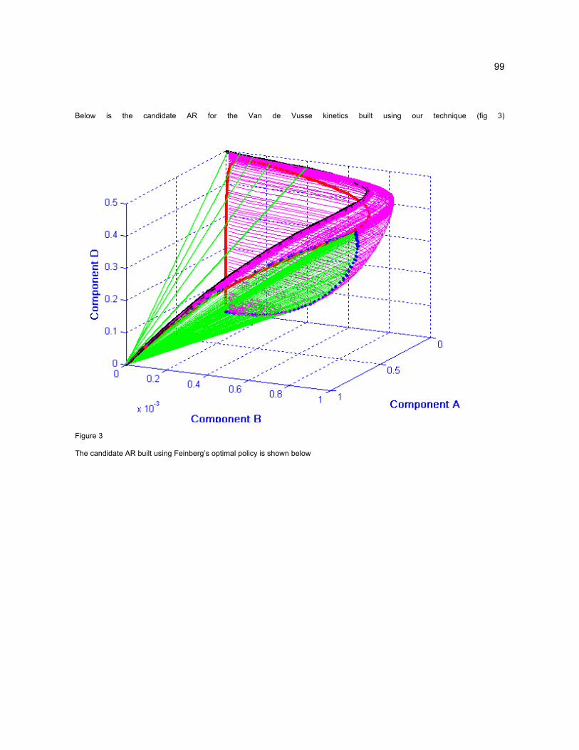
99
Below is the candidate AR for the Van de Vusse kinetics built using our technique (fig 3)
Figure 3
The candidate AR built using Feinberg’s optimal policy is shown below
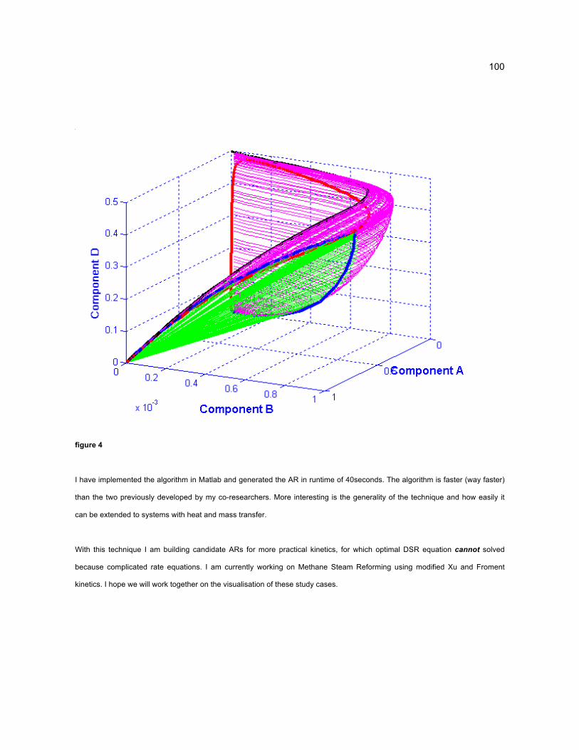
100
figure 4
I have implemented the algorithm in Matlab and generated the AR in runtime of 40seconds. The algorithm is faster (way faster)
than the two previously developed by my co-researchers. More interesting is the generality of the technique and how easily it
can be extended to systems with heat and mass transfer.
With this technique I am building candidate ARs for more practical kinetics, for which optimal DSR equation cannot solved
because complicated rate equations. I am currently working on Methane Steam Reforming using modified Xu and Froment
kinetics. I hope we will work together on the visualisation of these study cases.
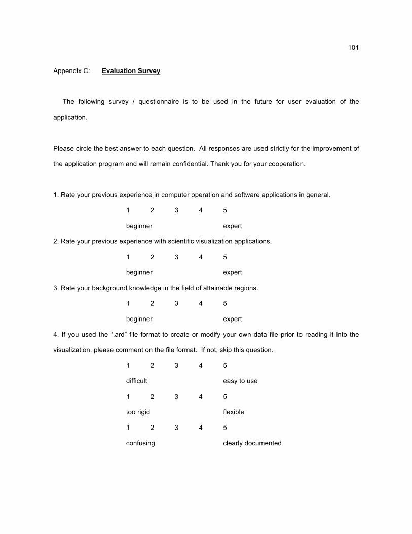
101
Appendix C: Evaluation Survey
The following survey / questionnaire is to be used in the future for user evaluation of the
application.
Please circle the best answer to each question. All responses are used strictly for the improvement of
the application program and will remain confidential. Thank you for your cooperation.
1. Rate your previous experience in computer operation and software applications in general.
1 2 3 4 5
beginner expert
2. Rate your previous experience with scientific visualization applications.
1 2 3 4 5
beginner expert
3. Rate your background knowledge in the field of attainable regions.
1 2 3 4 5
beginner expert
4. If you used the “.ard” file format to create or modify your own data file prior to reading it into the
visualization, please comment on the file format. If not, skip this question.
1 2 3 4 5
difficult easy to use
1 2 3 4 5
too rigid flexible
1 2 3 4 5
confusing clearly documented
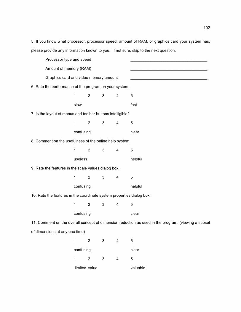
102
5. If you know what processor, processor speed, amount of RAM, or graphics card your system has,
please provide any information known to you. If not sure, skip to the next question.
Processor type and speed ___________________________________
Amount of memory (RAM) ___________________________________
Graphics card and video memory amount ___________________________________
6. Rate the performance of the program on your system.
1 2 3 4 5
slow fast
7. Is the layout of menus and toolbar buttons intelligible?
1 2 3 4 5
confusing clear
8. Comment on the usefulness of the online help system.
1 2 3 4 5
useless helpful
9. Rate the features in the scale values dialog box.
1 2 3 4 5
confusing helpful
10. Rate the features in the coordinate system properties dialog box.
1 2 3 4 5
confusing clear
11. Comment on the overall concept of dimension reduction as used in the program. (viewing a subset
of dimensions at any one time)
1 2 3 4 5
confusing clear
1 2 3 4 5
limited value valuable
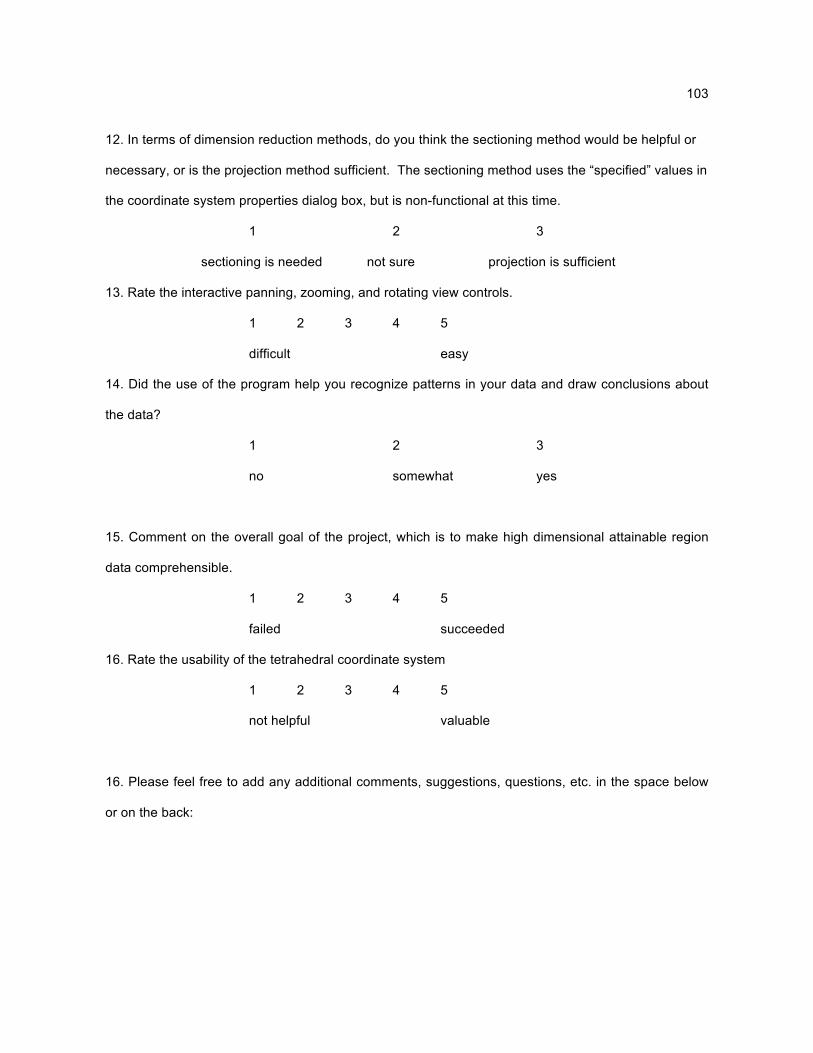
103
12. In terms of dimension reduction methods, do you think the sectioning method would be helpful or
necessary, or is the projection method sufficient. The sectioning method uses the “specified” values in
the coordinate system properties dialog box, but is non-functional at this time.
1 2 3
sectioning is needed not sure projection is sufficient
13. Rate the interactive panning, zooming, and rotating view controls.
1 2 3 4 5
difficult easy
14. Did the use of the program help you recognize patterns in your data and draw conclusions about
the data?
1 2 3
no somewhat yes
15. Comment on the overall goal of the project, which is to make high dimensional attainable region
data comprehensible.
1 2 3 4 5
failed succeeded
16. Rate the usability of the tetrahedral coordinate system
1 2 3 4 5
not helpful valuable
16. Please feel free to add any additional comments, suggestions, questions, etc. in the space below
or on the back:
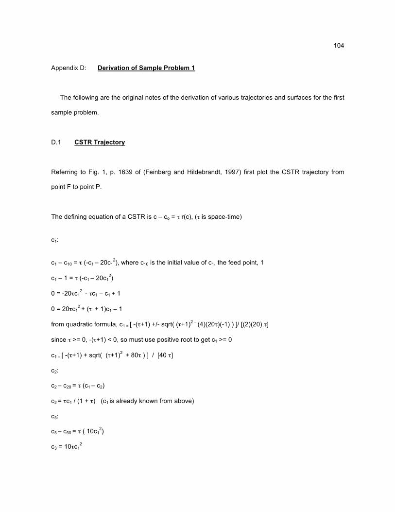
104
Appendix D: Derivation of Sample Problem 1
The following are the original notes of the derivation of various trajectories and surfaces for the first
sample problem.
D.1 CSTR Trajectory
Referring to Fig. 1, p. 1639 of (Feinberg and Hildebrandt, 1997) first plot the CSTR trajectory from
point F to point P.
The defining equation of a CSTR is c – co = " r(c), (" is space-time)
c1:
c1 – c10 = " (-c1 – 20c12), where c10 is the initial value of c1, the feed point, 1
c1 – 1 = " (-c1 – 20c12)
0 = -20"c12 - "c1 – c1 + 1
0 = 20"c12 + (" + 1)c1 – 1
from quadratic formula, c1 = [ -("+1) +/- sqrt( ("+1)2 – (4)(20")(-1) ) ]/ [(2)(20) "]
since " >= 0, -("+1) < 0, so must use positive root to get c1 >= 0
c1 = [ -("+1) + sqrt( ("+1)2 + 80" ) ] / [40 "]
c2:
c2 – c20 = " (c1 – c2)
c2 = "c1 / (1 + ") (c1 is already known from above)
c3:
c3 – c30 = " ( 10c12)
c3 = 10"c12
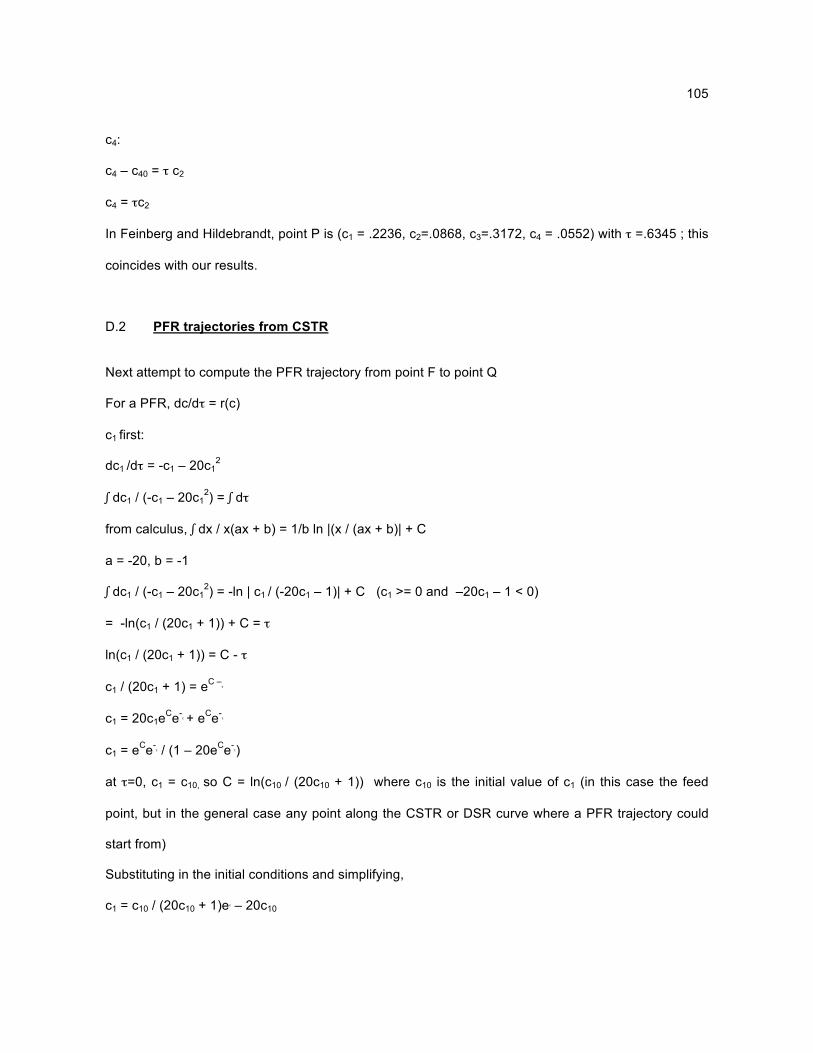
105
c4:
c4 – c40 = " c2
c4 = "c2
In Feinberg and Hildebrandt, point P is (c1 = .2236, c2=.0868, c3=.3172, c4 = .0552) with " =.6345 ; this
coincides with our results.
D.2 PFR trajectories from CSTR
Next attempt to compute the PFR trajectory from point F to point Q
For a PFR, dc/d" = r(c)
c1 first:
dc1 /d" = -c1 – 20c12
$ dc1 / (-c1 – 20c12) = $ d"
from calculus, $ dx / x(ax + b) = 1/b ln |(x / (ax + b)| + C
a = -20, b = -1
$ dc1 / (-c1 – 20c12) = -ln | c1 / (-20c1 – 1)| + C (c1 >= 0 and –20c1 – 1 < 0)
= -ln(c1 / (20c1 + 1)) + C = "
ln(c1 / (20c1 + 1)) = C - "
c1 / (20c1 + 1) = eC –"
c1 = 20c1eCe-" + eCe-
"
c1 = eCe-" / (1 – 20eCe-
")
at "=0, c1 = c10, so C = ln(c10 / (20c10 + 1)) where c10 is the initial value of c1 (in this case the feed
point, but in the general case any point along the CSTR or DSR curve where a PFR trajectory could
start from)
Substituting in the initial conditions and simplifying,
c1 = c10 / (20c10 + 1)e" – 20c10

106
However, computing c2, c3, and c4 became more difficult because the functions became difficult or
impossible to integrate directly. For example,
dc3 / d" = 10c12 = 10 c10
2 / [(20c10 + 1)e" – 20c10]2
Various integration methods such as substitution and integration by parts were attempted
unsuccessfully. So, a differential equation solver called Polymath was used to compute the solutions,
entering various initial conditions from the CSTR and DSR trajectory points and letting Polymath
compute the points of the resulting PFR trajectories. These points were produced by Polymath as one
text file per trajectory, which the application then read and parsed to get the points.
The system of ODE’s is:
dc1 / d" = -c1 – 20c12
dc2 / d" = c1 – c
dc3 / d" = 10 c12
dc4 / d" = c2
The ouput points are stored in files c0.txt – c21.txt in the data directory for the project.
D.3 DSR Trajectory
From (Feinberg, 2000), the governing equation of a DSR is
dc/d" = r(c) + #(c) (c0 – c)
where c0 is the side feed concentration, and #(c) is a function depending on the number of dimensions
of c
c0, the side feed concentration is (1,0,0), because the sample problem assumes an ample supply of
the original feed supply is available to use as side feed (given)
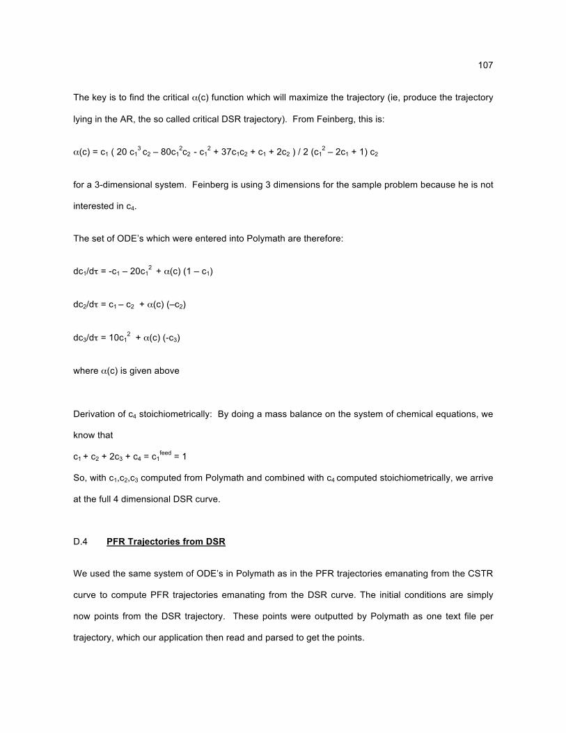
107
The key is to find the critical #(c) function which will maximize the trajectory (ie, produce the trajectory
lying in the AR, the so called critical DSR trajectory). From Feinberg, this is:
#(c) = c1 ( 20 c13 c2 – 80c1
2c2 - c12 + 37c1c2 + c1 + 2c2 ) / 2 (c1
2 – 2c1 + 1) c2
for a 3-dimensional system. Feinberg is using 3 dimensions for the sample problem because he is not
interested in c4.
The set of ODE’s which were entered into Polymath are therefore:
dc1/d" = -c1 – 20c12 + #(c) (1 – c1)
dc2/d" = c1 – c2 + #(c) (–c2)
dc3/d" = 10c12 + #(c) (-c3)
where #(c) is given above
Derivation of c4 stoichiometrically: By doing a mass balance on the system of chemical equations, we
know that
c1 + c2 + 2c3 + c4 = c1feed = 1
So, with c1,c2,c3 computed from Polymath and combined with c4 computed stoichiometrically, we arrive
at the full 4 dimensional DSR curve.
D.4 PFR Trajectories from DSR
We used the same system of ODE’s in Polymath as in the PFR trajectories emanating from the CSTR
curve to compute PFR trajectories emanating from the DSR curve. The initial conditions are simply
now points from the DSR trajectory. These points were outputted by Polymath as one text file per
trajectory, which our application then read and parsed to get the points.

108
The system of ODE’s we used is:
dc1 / d" = -c1 – 20c12
dc2 / d" = c1 – c2
dc3 / d" = 10 c12
dc4 / d" = c2
The output points are stored in files d0.txt – d25.txt in the data directory for the project.
109
VITA
NAME Thomas Peterka
EDUCATION University of Illinois at Chicago (UIC), Chicago, IL
Bachelor of Science, Computer Science Engineering June, 1987
HONORS Bell Honor Award for highest grade point average in the College of Engineering graduating class of 1987,5.0 / 5.0 GPA
RESEARCH Research assistant, Electronic Visualization Laboratory (EVL) at UIC. PROFESSIONAL Tau Beta Pi National Engineering Honor Society AFFILIATIONS Phi Kappa Phi National Honor Society