scientific journal of the ternopil national...
TRANSCRIPT

Вісник Тернопільського національного технічного університету
Scientific Journal of the Ternopil National Technical University
2016, № 1 (81)
ISSN 1727-7108. Web: visnyk.tntu.edu.ua
SCIENTIFIC JOURNAL OF THE TERNOPIL
NATIONAL TECHNICAL UNIVERSITY
Scientific Journal
Issued 4 times a year
Founded in September, 1996
№ 1 (81) 2016 Founder and publisher:
Ternopil Ivan Puluj National Technical University
List of journals ISSN 1727-7108
Copyright 10.06.2010 КВ № 16861-5624ПР
Recommended by the Scientific Council of the Ternopil Ivan Puluj National
Technical University, Protocol No 2, 22.03.2016
Editorial board: P.V. Yasniy (Editor-in-Chief), R.М. Rogatynskyi (Associate Editor), B.G. Shelestovskyi (Executive Editor), О.Ye. Andreikiv, V.А. Andriychuk, Z.Ya. Blikharskyi, М.І. Bobyr, B.М. Gevko, L.D. Didukh, Ya.P. Dragan, P.S. Yevtukh, М.P. Karpinskyi, V.А. Kryven, R.М. Kushnir, Yu.M. Lapusta, V.S. Loveikin, S.А. Lupenko, І.V. Lutsiv, J.J. Luchko, P.О. Marushchak, М.S. Mykhailyshyn, Z.Т. Nazarchuk, G.М. Nykyforchyn, М.R. Petryk, М.І. Pylypets, М.І. Pidgurskyi, М.V. Pryimak, Ch.V. Pulka, Т.І. Rybak, M.S. Stechyshyn, P.D. Stukhlyak, G.Т. Sulym, V.T. Troshchenko, О.М. Shabliy, B.І. Yavorskyi.
International editorial board: J. Fraissard (France), J. Kaleta (Poland), T. Lentla (Ectonia), G. Pluvinage (France),
K. Smedley (USA), L. Tóth (Hungary).
Editorial office address: Ternopil Ivan Puluj National Technical University,
56, Ruska Str. Ternopil 46001, Ukraine. Tel. (380) 0352 255798, (380) 352 253585. Fax: (380) 352 254983. E-mail: [email protected]
WWW-address: visnyk.tntu.edu.ua
Managing Editor A.V. Grytskiv; Ye.I. Grytsenko
Art Editor, design, typist О.A. Dzyaduk
ISSN 1727-7108
Ternopil Ivan Puluj National
Technical University, 2016

CONTENT
2
ВІСНИК ТЕРНОПІЛЬСЬКОГО
НАЦІОНАЛЬНОГО ТЕХНІЧНОГО УНІВЕРСИТЕТУ
Науковий журнал
Виходить 4 рази у рік
Заснований у вересні 1996 р.
№ 1 (81) 2016 р.
Засновник і видавець:
Тернопільський національний технічний університет імені Івана Пулюя
Реєстраційний номер ISSN 1727-7108
Свідоцтво про державну реєстрацію друкованого засобу масової інформації
серії КВ № 16861-5624ПР від 10.06.2010 р.
Рекомендовано до друку вченою радою Тернопільського національного
технічного університету імені Івана Пулюя 22.03.2016 р., протокол № 2.
Редакційна колегія
П.В. Ясній (головний редактор), Р.М. Рогатинський (заст. головного редактора),
Б.Г. Шелестовський (відповідальний секретар), О.Є. Андрейків, В.А. Андрійчук,
З.Я. Бліхарський, М.І. Бобир, Б.М. Гевко, Л.Д. Дідух, Я.П. Драган,
П.С. Євтух, М.П. Карпінський, В.А. Кривень, Р.М. Кушнір, Ю.М. Лапуста,
В.С. Ловейкін, С.А. Лупенко, І.В. Луців, Й.Й. Лучко, П.О. Марущак,
М.С. Михайлишин, З.Т. Назарчук, Г.М. Никифорчин, М.Р. Петрик,
М.І. Пилипець, М.І. Підгурський, М.В. Приймак, Ч.В. Пулька, Т.І. Рибак,
М.С. Стечишин, П.Д. Стухляк, Г.Т. Сулим, В.Т. Трощенко, О.М. Шаблій ,
Б.І. Яворський.
Міжнародна редакційна колегія
Є. Калєта (Польща), Т. Лехтла (Естонія), Ґ. Плювінаж (Франція),
К. Смедлі (США), Л. Тот (Угорщина), Ж. Фресад (Франція). Адреса редакції: 46001, Тернопіль, вул. Руська, 56.
Тернопільський національний технічний університет імені Івана Пулюя. Телефони: (0352) 255798, 253585, факс: (0352) 254983. E-mail: [email protected]
WWW-address: visnyk.tntu.edu.ua
Редактори: А.В. Грицьків; Є.І. Гриценко
Комп’ютерне макетування О.А. Дзядик
ISSN 1727-7108
Тернопільський національний технічний
університет імені Івана Пулюя, 2016

CONTENT
ISSN 1727-7108. Scientific Journal of the TNTU, No 1 (81), 2016 …………………………………………………………. 3
CONTENT
MECHANICS AND MATERIALS SCIENCE
Oleksandr Bahno. Wave propagation in the pre-deformed compressible elastic layer interacting with a layer of viscous compressible liquid ………………………………… 7
Natalia Shevtsova, Andrii Syaskyi. Stress distribution in an infinite orthotropic plate with partly reinforced elliptical contour …………………………..…………………… 15
Mykhailo Dudyk. Destruction zone near the tip of interfacial crack at a prevailing tensile loading ……...……………………………………………….…......................... 21
Bogdan Drobenko, Aleksander Buryk. Evaluation of fire resistance of structural elements considering nonlinearity of deformation processes during fire …..………….. 29
Oleksandr Bezverkhyi, Ludmila Grigoryeva, Sergiy Grigoryev. Resonance radial oscillations of a piezoceramic cylinders and spheres taking into account electromechanical losses ……………………………………..………………………… 41
Iaroslav Dubyk, Igor Orynyak. Fluid-structure interaction in free vibration analysis of pipelines ……………………………………………………………………………….. 49
MANUFACTURING ENGINEERING AND AUTOMATED PROCESSES
Ihor Lutsiv, Volodymyr Sharyk, Oleksandr Stakhurskiy, Dmytro Dyachuk. Analysis of dynamics of adaptive three edge heads with elastic guides and electromagnetic drives 59
Timothii Rybak, Oksana Oryshchyn, Taras Dovbush, Anatolii Dovbush. Energy and integrated method in evaluation of working life of supporting systems for mobile agricultural machines ………………………………………………………………….. 70
Roman Hevko, Yuriy Dzyadykevych, Ihor Tkachenko, Serhii Zalutskyi. Parameter justification for interworking relationship of elastic screw operating element with grain material …………………………………………………………………....…………… 77
Yakiv Nemyrovskyy, Oleksandr Chernyavskyy, Pavlo Yeryomin, Yuriy Tsekhanov. Issues about limit plastic deformations of deforming broaching of cast iron parts ……. 88
INSTRUMENT-MAKING
AND INFORMATION-MEASURING SYSTEMS
Petro Yevtukh, Oleksandr Vakulenko. Features of statistical data processing at insulation testing of enameled electric wires ………………………………………….. 98
Roman Mykhailyshyn, Yaroslav Prots’, Volodymyr Savkiv. Optimization of bernoulli gripping device’s orientation under the process of manipulations along direct trajectory 107
Oleksandr Osloinskyy. Error of methodical study at measurement of average energy consumption of microcontrollers ……………………………………..………………... 118

CONTENT
4 ……………………………………………….…………... ISSN 1727-7108. Scientific Journal of the TNTU, No 1 (81), 2016
MATHEMATICAL MODELING.
MATHEMATICS
Yurii Chui, Petro Martynyuk. Finite element method in spatial filtration consolidation
problem with thin semi-permeable inclusions under the influence of the heat and salt
transfer …….………………………………..……......................................................... 125
Tetyana Solyar. Ways to improve fourier series convergence and its application for
laplace numerical inversion …………………………..………………………............... 136
IN COMMEMORATION OF DR. OLEH M. SHABLIY .......................................... 145

ЗМІСТ
ISSN 1727-7108. Вісник ТНТУ, № 1 (81), 2016 ……………………..…………………………………………………………….. 5
ЗМІСТ
МЕХАНІКА ТА МАТЕРІАЛОЗНАВСТВО
Олександр Багно. Поширення хвиль у попередньо деформованому стисливому
пружному шарі, який взаємодіє з шаром в’язкої стисливої рідини ……………….. 7
Наталія Шевцова; Андрій Сяський. Розподіл напружень у нескінченній
ортотропній пластинці з частково підсиленим еліптичним контуром .…………… 15
Михайло Дудик. Зона деструкції біля вершини міжфазної тріщини при
переважаючих розтягувальних навантаженнях ………………..…………………… 21
Богдан Дробенко; Олександр Бурик. Оцінювання вогнетривкості елементів
конструкцій з урахуванням нелінійності процесів їх деформування ……..………. 29
Олександр Безверхий; Людмила Григор’єва; Сергій Григор’єв. Резонансні
радіальні коливання п’єзокерамічних циліндрів та куль з врахуванням
електромеханічних втрат ……………………………………..……………………… 41
Ярослав Дубик; Ігор Ориняк. Врахування взаємодії середовище-трубопровід при
аналізі власних частот трубопровідної системи ……………………………………. 49
МАШИНОБУДУВАННЯ, АВТОМАТИЗАЦІЯ ВИРОБНИЦТВА
ТА ПРОЦЕСИ МЕХАНІЧНОЇ ОБРОБКИ
Ігор Луців; Володимир Шарик; Олександр Стахурський; Дмитро Дячук.
Аналіз динаміки трирізцевих головок з пружними напрямними і
електромагнітними приводами ………………..…….………………………..……... 59
Тимофій Рибак; Оксана Орищин; Тарас Довбуш; Анатолій Довбуш. Енергетично інтегральний метод оцінки ресурсу роботи несучих систем
мобільних сільськогосподарських машин …………………………………….......... 70
Роман Гевко; Юрій Дзядикевич; Ігор Ткаченко; Сергій Залуцький.
Обгрунтування параметрів взаємодії еластичного гвинтового робочого органу із
зерновим матеріалом …...…………………………………………….......................... 77
Яків Немировський; Олександр Чернявський; Павло Єрьомін; Юрій Цеханов.
До питання про граничні пластичні деформації заготовок із чавуну, оброблених
деформувальним протягуванням ………………………………..…………………... 88
ПРИЛАДОБУДУВАННЯ ТА ІНФОРМАЦІЙНО ВИМІРЮВАЛЬНІ
СИСТЕМИ
Петро Євтух; Олександр Вакуленко. Особливості оброблення статистичних
даних при випробуваннях ізоляції емальованих електричних проводів ..…............ 98
Роман Михайлишин; Ярослав Проць; Володимир Савків. Оптимізація
орієнтації струминного захоплювального пристрою в процесі маніпулювання по
прямій траєкторії ……………………………………………………………………... 107

ЗМІСТ
6……………………………………………….……………………………… ISSN 1727-7108. Вісник ТНТУ, № 1 (81), 2016
Олександр Осолінський. Дослідження методичної похибки при вимірюванні
середнього енергоспоживання мікроконтролерів ………………………………….. 118
МАТЕМАТИЧНЕ МОДЕЛЮВАННЯ. МАТЕМАТИКА
Юрій Чуй; Петро Мартинюк. Метод скінченних елементів у просторовій задачі
фільтраційної консолідації грунтів з тонкими напівпроникними включеннями в
умовах впливу теплосолеперенесення ………………………………………………. 125
Тетяна Соляр. Спосіб покращення збіжності рядів Фур’є та його застосування
для числового обернення перетворення Лапласа …………………………………… 136
ПАМ’ЯТІ ОЛЕГА МИКОЛАЙОВИЧА ШАБЛІЯ ……………………………... 145

Вісник Тернопільського національного технічного університету
Scientific Journal of the Ternopil National Technical University
2016, № 1 (81)
ISSN 1727-7108. Web: visnyk.tntu.edu.ua
Corresponding author: Oleksandr Bahno; e-mail: [email protected] ………………………………………………………… 7
MECHANICS AND MATERIALS SCIENCE
МЕХАНІКА ТА МАТЕРІАЛОЗНАВСТВО
UDC 539.3
WAVE PROPAGATION IN THE PRE-DEFORMED COMPRESSIBLE
ELASTIC LAYER INTERACTING WITH A LAYER OF VISCOUS
COMPRESSIBLE LIQUID
Oleksandr Bahno
S.P. Tymoshenko Institute of Mechanics. National Academy of Sciences of
Ukraine, Kyiv, Ukraine
Resume. Based on three-dimensional equations of linearized elasticity theory for finite deformations of
elastic body and three-dimensional linearized Navier-Stokes equations for the liquid medium, the problem of
propagation of acoustic waves in preliminarily deformed compressible elastic layer in contact with a layer of
viscous compressible liquid has been formulated. A numerical study is conducted, dispersion curves are
constructed and dependencies of the phase velocities and attenuation coefficients modes to the thickness of layers
of elastic body and a viscous compressible liquid in a wide frequency range are determined. An effect of initial
stresses on phase-frequency spectrum of waves in the hydroelastic system is analyzed.
Keywords: compressible elastic layer, layer of viscous compressible liquid, initial stresses, harmonic
waves.
Received 26.11.2015
Problem setting. The development of science and technology brings new increased
requirements for research in hydro elasticity and in particular to study wave propagation in
elastic bodies in contact with the liquid. There is a strong need for comprehensive consideration
of real solid and liquid media properties and on this basis adequate description of different
phenomena and mechanical effects that characterize dynamic processes in hydroelastic
waveguides.
Analysis of the known research results. The waves propagating along the contact
boundary of elastic layer and the layer of liquid are among thoroughly studied generalized basic
types of acoustic waves, such as Rayleigh, Stoneley Lyave and Lamb waves. Work reviews and
analysis of results obtained within classical elasticity theory and models of ideal compressible
liquid are given in [1]. However, considerable practical use of surface waves raises the problem
of taking into account real medium properties. Among these factors are the initial tensions and
viscosity of the liquid. Tasks examined and results obtained on the basis of the properties of
solids and liquids are given in [2, 3].
The purpose of the work. Explore the dispersion spectrum of wave process in a pre-
stressed compressible layer – layer of viscous compressible liquid system based on three-
dimensional linearized Navier-Stokes equations for the liquid medium and three-dimensional
linearized elasticity equations for finite deformation of solids in the most complex theoretical
as well as important applied aspect of the case, which covers long-wave and short-wave part of
the spectrum.
Formulation of the problem. In this paper, to study wave propagation in a liquid
layer – elastic layer system a model is involved that takes into account the initial deformation
of solids, together with a model of viscous compressible Newtonian liquid. It uses three-

Wave propagation in the pre-deformed compressible elastic layer interacting with a layer of viscous compressible liquid
8 ………………………….…………….………………….… ISSN 1727-7108. Scientific Journal of the TNTU, No 1 (81), 2016
dimensional equations of linearized elasticity theory at finite deformations of solids and three-
dimensional linearized Navier-Stokes equations for the liquid at rest without taking into account
thermal effects. The approach chosen applies problem formulation and the method based on the
use of representations of general solutions to the equations of motion of an elastic compressible
body and a viscous compressible liquid proposed in works [4 – 10].
In the case of homogeneous stress-tension state coefficients in the equations for compressible
elastic bodies are constants values that provide a representation of general solutions. For flat
case under consideration, the general solution will have the form [4 – 10]
(1)
, (2)
where introduced functions satisfy equation
(3)
(4)
(5)
This problem has the following dynamic
(6)
and kinematic
(7)
boundary conditions. Here are the following notation: – the components of the elastic body
travel vector; – extension of the elastic layer in the directions of coordinate axes; and
– values which are determined from equations of state and depend on the type of elastic
;zz
u21
12
1
;tsazsa
s
za
sau 12
2
0
1111
2
1
2
1
2
2
2
0
1111
2
1
2
1
0
2212
2
1
2
2
2
1
2
1212
2
2
0
1111
2
1
2
;tztz
v
2
3
2
1
2
2
1
tztzv
1
3
2
2
2
2
2
i
22
2
01112
22
21
02222
22
22
21
2
2
2
01111
21
21
22
2
01111
21
21
02212
21
22
21
2
zs
sa
ztsazsa
s
z
242 42 12 12
12 2 22 2 0 2 0 2 0
1 21 1 12 11 1 11 11 2 12 11
0;a
t z zs a s s
;tazzta
*
01
3
41 22
2
2
0
2
2
2
2
1
2
2
0
2 2
*
32 2
1 2
0.t z z
;QP zz 0101 22 ;QP zz 0202 22 ;Q hz 0221 ;Q hz 0
222
;P hz 0121 0
122 hzP
;t
uv zz 02
1
021
0
202 22
zz
t
uv
іu
і ija
ij

Oleksandr Bahno
ISSN 1727-7108. Вісник ТНТУ, № 1 (81), 2016 ……………………..…………………………………………………………….. 9
potential [11]; – initial stresses ( ); – elastic layer matter density; –
the components of liquid velocity vector; and – kinematic and dynamic viscosity of the
liquid; and – the density and speed of sound in a liquid at rest. and
– the
components of the stress in a solid and a liquid.
Then parameters, characterizing the propagation of waves, are sought in the class of
traveling waves, presented as
(8)
where – wave number; – wave attenuation coefficient; – circular
frequency.
Note that chosen for this research class of harmonic waves, being the most simple and
convenient in theoretical studies, does not limit the generality of the results obtained as a linear
wave of arbitrary shape is known to be represented by a set of harmonic components. Then two
Sturm-Liouville problems on eigenvalues for equations of travel of an elastic body and liquid
are considered. On solving the equations their respective functions are found. After substitution
of the solutions into boundary conditions (6) – (7) we get a system of linear homogeneous
algebraic equations with reference to integration constants. Based on the conditions of a
nontrivial solution existence, and equating the system determinant to zero, we get the dispersion
equation
, (9)
where is the phase velocity of waves in hydroelastic system; – shear wave
velocity in the elastic body material; – shear modulus; – thickness layer of the viscous
liquid; – thickness of the elastic layer.
As is known in unlimited compressible elastic body both longitudinal and shear waves
exist. In an ideal compressible liquid medium only longitudinal waves spread. Longitudinal as
well as and shear waves exist in a viscous compressible liquid. These waves interact in free
boundary surfaces, as well as in media contact surfaces, generating a complex wave field in
hydroelastic system. Waves, thus created, spread with dispersion. Their phase velocities are in
some way dependent on the frequency.
Note that the resulting dispersion equation (9) does not depend on the form of elastic
potential. It is the most general and it is possible to obtain a number of partial cases considered
in [2, 12 – 14].
Analysis of numerical results. Subsequently the dispersion equation (9) was solved
numerically. Herewith the calculations were made for a system of organic glass – water, which
is characterized by the following parameters: resilient layer kg/m3, Pa;
liquid layer kg/m3, m/s,
Murnahan form of three-invariant potential was used in numerical realization of a
problem for organic glass [11]. With this in view, Murnahan constants for organic glass through
which equation values of state and state, were defined as follows [11, 12]:
Pa; Pa; Pa.
The results of calculations are presented in Figures 1 – 8.
0
iii
ii
ііs2
0
3210
іv
* *
0 0a jQ jP
,tkziexpzX jj 12 ,,j 31
k ik
,c/h,c/h,,а,,s,,a,,cedet ss
*
iiijijlm 02100
0 81,m,l
с )c(c ss 2
1h
2h
11609
10861 ,
10000 514590 ,а ,,caa s 1526100 .,*
0010
ija ij9
10913 ,a
910027 ,b
910411 ,c

Wave propagation in the pre-deformed compressible elastic layer interacting with a layer of viscous compressible liquid
10 ………………………….…………….………………….… ISSN 1727-7108. Scientific Journal of the TNTU, No 1 (81), 2016
For the elastic layer which does not interact with the liquid Fig. 1 shows dependencies
of dimensionless values of phase velocities of Lamb waves on dimensionless
thickness of the elastic layer (frequency) ( ) in the absence of initial
deformations. Numbers indicate antisymmetric modes and – symmetrical modes
accordingly.
Fig. 2 shows the dispersion curves for hydroelastic waveguide showing the
dependencies of dimensionless values of phase velocities modes on dimensionless value of
viscous liquid thickness ( ) for the elastic layer with a thickness equal to
and in the absence of initial deformations.
Curves for hydroelastic waveguide showing the dependencies of dimensionless values
of mode attenuation coefficients on dimensionless thickness of viscous liquid elastic
layer with a thickness that equals also in the absence of initial deformations, shown in
Fig. 3 – 4.
The nature of the impact of preliminary tension on the phase velocities
modes in an elastic layer that interacts with a layer of viscous liquid graphics is illustrated by
Fig. 5 – 6, showing the dependencies of the change in the relative phase velocities
( ; – phase velocities of modes in hydroelastic system of pre-stressed layer,
– phase velocities of modes in hydroelastic system in the absence of initial deformations) on
the thickness of viscous liquid layer for the first 11 modes. These Figures show hydroelastic
waveguide dispersion curves, with its elastic layer thickness equal to .
The nature of the impact of preliminary tension on the attenuation
coefficients of modes in an elastic layer that interacts with a layer of viscous liquid is illustrated
on diagrams in Fig. 7 – 9, which shows attenuation coefficient relative value changes
dependencies ( , – mode attenuation coefficients in hydroelastic system with
pre-stressed layer; – mode attenuation coefficients in hydroelastic system in the absence of
initial deformations) on the viscous liquid thickness for the first 11 modes. These Figures show
curves for hydroelastic waveguide with a thick elastic layer, whose thickness is .
Research results. From the graphs presented in Fig. 1, it follows that the speed of zero
antisymmetric Lamb mode with increasing thickness of the elastic layer (frequency) tends
to Rayleigh wave velocity ( ) from below, and of zero symmetrical
mode speed tends to Rayleigh wave velocity ( ) from above. Speeds of all
higher Lamb modes with increasing thickness of the elastic layer (frequency) tend to shear wave
velocity in the material of the elastic body .
Charts for hydroelastic systems, which are shown in Fig. 2, in the case of thick elastic
layer with show that with increasing thickness of the layer of viscous compressible
liquid zero antisymmetric mode velocity tends to Stoneley wave velocity
( ), and zero symmetrical mode velocity tends to Rayleigh wave velocity
( ). By increasing the thickness of the liquid layer the first antisymmetric mode
speed tends to wave velocity , the value of which is less than the speed of sound in a
liquid ( ). Phase velocities of all other higher modes tend to the speed of sound
in a liquid medium .
c )сcc( s
2h schh 22
аn sn
c
1h schh 11 ,h 102
1h
102 h
),( 00400
11
cс
ссс
с
с
102 h
),( 00400
11
102 h
2h
Rc 933560,ccc sRR
Rc 933560,cR
sc
102 h
stc 76910,сcc sstst
Rc 933560,cR
12861,c
0a 152610 ,a
0a

Oleksandr Bahno
ISSN 1727-7108. Вісник ТНТУ, № 1 (81), 2016 ……………………..…………………………………………………………….. 11
Figure 1. Dependencies of dimensionless phase
velocities of Lamb normal waves on the
dimensionless thickness of elastic layer in
absence of the initial stresses
Figure 2. Dependencies of dimensionless phase
velocities of modes on the dimensionless thickness of
layer of viscous compressible liquid in absence of the
initial stresses
Figure 3. Dependencies of dimensionless
attenuation coefficients of modes
and on the dimensionless thickness of layer
of viscous compressible liquid in absence of the
initial stresses
Figure 4. Dependencies of dimensionless attenuation
coefficients of modes 3 – 7 on the dimensionless
thickness of layer of viscous compressible liquid in
absence of the initial stresses
Charts in Fig. 2 show that in hydroelastic waveguide with an elastic layer of a given
thickness with increasing thickness of the liquid layer higher modes velocities tend to the speed of sound in the liquid, which for the considered hydroelastic systems with selected
mechanical parameters is greater than shear wave velocity in solid material ( ).
From the graphs presented in Fig. 3 – 4, it follows, that liquid layers of a certain thickness and certain frequencies, for which mode attenuation coefficients take minimum as well as maximum value, exist for all modes. However, for modes 3 – 7 generated by a liquid medium, there are not only certain frequencies, but also the frequency range in which the modes spread with both the smallest and the biggest fading.
Figure 5. Dependencies of relative changes of
phase velocities of modes and on
the dimensionless thickness of layer of viscous
compressible liquid in presence of the initial
stretching
Figure 6. Dependencies of relative changes of
phase velocities of modes 3 – 7 on the
dimensionless thickness of layer of viscous
compressible liquid in presence of the initial
stretching
asasa ,,,, 21100
s2
2h 1h
sca 0
asa ,, 100 s1 ,, sa 22

Wave propagation in the pre-deformed compressible elastic layer interacting with a layer of viscous compressible liquid
12 ………………………….…………….………………….… ISSN 1727-7108. Scientific Journal of the TNTU, No 1 (81), 2016
From the charts shown in Fig. 5 – 6, it follows that the initial tension of elastic layer
causes an increase in phase velocities of zero and first antisymmetric and symmetric modes.
Speeds of all higher modes 3 – 7, generated by a layer of liquid in the vicinity of the frequencies
of their origin have less velocities of relevant modes in a layer without initial stresses. The
impact of the initial tension on the phase velocities of all modes with increasing thickness of
the liquid is reduced. It is easy to see that starting with the second mode and onwards on all
subsequent there are certain liquid layer thickness and frequencies at which the pre-deformation
does not affect their phase velocity. This qualitatively new pattern, which is absent in the case
of wave propagation in unbounded and semibounded bodies, was first discovered for the elastic
layer that does not interact with the liquid and is presented in work [12]. In the case of thick
elastic layer considered here every mode 3 – 7, generated by liquid, has three such frequencies.
We also note that from the charts in Fig. 7 and 8 imply the existence for all modes except
, viscous liquid layers of a certain thickness and certain frequencies at which the pre-
deformation does not affect attenuation coefficients of these modes.
Figure 7. Dependencies of relative changes of
attenuation coefficients of modes and
on the dimensionless thickness of layer of
viscous compressible liquid in presence of the
initial stretching
Figure 8. Dependencies of relative changes of
attenuation coefficients of modes and
3 – 7 on the dimensionless thickness of layer of
viscous compressible liquid in presence of the
initial stretching
Note that the chosen approach, results obtained and identified patterns of mode
dispersion spectrum allow for wave processes to set limits of using the models based on
different versions of small initial deformations theory as well as perfect liquid model. The
results can also be used in ultrasonic non-destructive method of determining the stresses in the
surface layers of materials [15] as well as in areas such as seismology, seismic prospecting
etc. [11]
Conclusions. Within the framework of the three-dimensional equations of the linearized
elasticity theory of finite deformations for the elastic body and three-dimensional linearized
Navier-Stokes equations for a viscous liquid of the problem of propagation of acoustic waves
in a pre-deformed compressible elastic layer, that interacts with a layer of viscous compressible
liquid, was presented. The influence of the initial deformation, the thicknesses of the layers of
the elastic body and liquid on the phase velocities and the attenuation coefficients of modes
were analyzed. The dispersion curves for the modes in a wide range of frequencies were given.
For hydroelastic system it was shown, that with increast of the thickness layer of viscous liquid
the velocity of zero antisymmetric mode tends to the Stoneley wave velocity and velocity of
zero symmetric mode tends to the Rayleigh wave velocity. By increasing of the thickness of
the liquid layer, the velocity of the first antisymmetric mode tends to the wave velocity, the
value of which is less than the velocity of sound in the liquid. The phase velocities of all other
higher modes tends to the velocity of sound in the liquid. It was determined that the initial
tension of the elastic layer leads to the increasing the phase velocities of zero and first
antisymmetric and symmetric modes. The velocities of all higher modes which were generated
s0
sa ,00 a1sas ,, 221

Oleksandr Bahno
ISSN 1727-7108. Вісник ТНТУ, № 1 (81), 2016 ……………………..…………………………………………………………….. 13
by a layer of liquid in the vicinity of the frequency of their origin are less than relevant velocities
in a layer without initial stresses. The effect of the initial tension on the phase velocities of all
modes decreases with the increase of layer thickness of the liquid. It was determined that for
all the modes, beginning with the second, there exist thicknesses the liquid layer and the certain
frequencies, at which the initial tension of the elastic layer has no effect on their phase velocities
and attenuation coefficients. It was shown that in the case of thick elastic layer every mode that
was generated by the liquid has three such frequencies. An approach developed and the results
obtained allow to establish for the wave processes the limits applicability of the models based
on different versions of the theory of small initial deformations, as well the model of an ideal
liquid. The results can be well used in the ultrasonic non-destructive method determination of
stresses in near-the-surface layers of materials as well as in areas such as seismology, seismic,
etc.
References
1. Viktorov I.A. Zvukovye poverkhnostnye volny v tverdykh telakh, Moskva, Nauka, 1981, 288 p.
[in Russian].
2. Bagno A.M., Guz A.N. Elastic waves in pre-stressed bodies interacting with a fluid (survey), Int. Appl.
Mech., Vol. 33, No. 6, 1997, P. 435 – 463.
3. Ottenio M., Destrade M., Ogden R.W. Acoustic waves at the interface of a pre-stressed incompressible
elastic solid and a viscous fluid, Int. J. of Non-Linear Mech., Vol. 42, No. 2, 2007, P. 310 – 320.
4. Huz A.N. O zadachakh aerohidroupruhosti dlia tel s nachalnymi napriazheniiami, Prikladnaia
mekhanika, Vol. 16, No. 3, 1980, P. 3 – 21. [in Russian].
5. Huz A.N. Upruhie volny v telakh s nachalnymi napriazheniiami, V 2-kh tomakh, Kiev, Naukova
dumka, 1986. [in Russian]. 6. Huz A.N. Dinamika szhimaemoi viazkoi zhidkosti, Kiev, A.S.K., 1998, 350 p. [in Russian].
7. Huz A.N. A.N. Upruhie volny v telakh s nachalnymi (ostatochnymi) napriazheniiami, Kiev, A.S.K., 2004,
672 p. [in Russian].
8. Guz A.N. Compressible, viscous fluid dynamics (review). Part 1, Int. Appl. Mech., Vol. 36, No. 1, 2000,
P. 14 – 39.
9. Guz A.N. The dynamics of a compressible viscous liquid (review). II, Int. Appl. Mech., Vol. 36, No. 3,
2000, P. 281 – 302.
10. Guz A.N. Dynamics of compressible viscous fluid, Cambridge Scientific Publishers, 2009, 428 p.
11. Huz A.N., Makhort F.H., Hushcha O.I. Vvedenie v akustoupruhost, Kiev, Naukova dumka, 1977, 152 p.
[in Russian].
12. Huz A.N., Zhuk A.P., Makhort F.H. Volny v sloe s nachalnymi napriazheniiami, Kiev, Naukova dumka,
1976, 104 p. [in Russian].
13. Babich S.Y., Huz A.N., Zhuk A.P. Upruhie volny v telakh s nachalnymi napriazheniiami, Prikladnaia
mekhanika, Vol. 15, No. 4, 1979, P. 3 – 23. [in Russian].
14. Zhuk A.P. Volny Stonli v srede s nachalnymi napriazheniiami, Prikladnaia mekhanika, Vol. 16, No. 1,
1980, P. 113 – 116. [in Russian].
15. Guz A.N. On the foundations of the ultrasonic non-destructive determination of stresses in near-the-surface
layers of materials. Review, J. Phys. Science and Application, Vol. 1, No. 1, 2011, P. 1 – 1
Список використаної літератури
1. Викторов, И.А. Звуковые поверхностные волны в твердых телах [Текст] / И.А. Викторов – М.:
Наука, 1981. – 288 с.
2. Bagno, A.M. Elastic waves in pre-stressed bodies interacting with a fluid (survey) / A.M. Bagno,
A.N. Guz // Int. Appl. Mech. – 1997. – № 6 (33). – P. 435 – 463.
3. Ottenio, M. Acoustic waves at the interface of a pre-stressed incompressible elastic solid and a viscous
fluid / M. Ottenio, M. Destrade, R.W. Ogden // Int. J. of Non-Linear Mech. – 2007. – № 2 (42). – P. 310 – 320.
4. Гузь, А.Н. О задачах аэрогидроупругости для тел с начальными напряжениями [Текст] / А.Н. Гузь //
Прикладная механика. – 1980. – № 3 (16). – С. 3 – 21.
5. Гузь, А.Н. Упругие волны в телах с начальными напряжениями: в 2 т. [Текст] / А.Н. Гузь. – К.: Наук.
думка, 1986. Т. 1: Общие вопросы. – 376 с. Т. 2: Закономерности распространения. – 536 с.
6. Гузь, А.Н. Динамика сжимаемой вязкой жидкости [Текст] / А.Н. Гузь. – К.: А.С.К., 1998. – 350 с.
7. Гузь, А.Н. Упругие волны в телах с начальными (остаточными) напряжениями [Текст] /
А.Н. Гузь. – К.: А.С.К., 2004. – 672 с.

Wave propagation in the pre-deformed compressible elastic layer interacting with a layer of viscous compressible liquid
14 ………………………….…………….………………….… ISSN 1727-7108. Scientific Journal of the TNTU, No 1 (81), 2016
8. Guz, A.N. Compressible, viscous fluid dynamics (review). Part 1 / A.N. Guz // Int. Appl. Mech. – 2000. –
№ 1 (36). – P. 14 – 39.
9. Guz, A.N. The dynamics of a compressible viscous liquid (review). II / A.N. Guz // Int. Appl. Mech. –
2000. – № 3 (36). – P. 281 – 302.
10. Guz, A.N. Dynamics of compressible viscous fluid. / A.N. Guz – Cambridge Scientific Publishers, 2009. –
428 p.
11. Гузь, А.Н. Введение в акустоупругость [Текст] / А.Н. Гузь, Ф.Г. Махорт, О.И. Гуща. – К.: Наук.
думка, 1977. – 152 с.
12. Гузь, А.Н. Волны в слое с начальными напряжениями [Текст] / А.Н. Гузь, А.П. Жук, Ф.Г. Махорт. –
К.: Наук. думка, 1976. – 104 с.
13. Бабич, С.Ю. Упругие волны в телах с начальными напряжениями [Текст] / С.Ю. Бабич, А.Н. Гузь,
А.П. Жук // Прикладная механика. – 1979. – № 4 (15). – С. 3 – 23.
14. Жук, А.П. Волны Стонли в среде с начальными напряжениями [Текст] / А.П. Жук // Прикладная
механика. – 1980. – № 1 (16). – С. 113 – 116.
15. Guz, A.N. On the foundations of the ultrasonic non-destructive determination of stresses in near-the-surface
layers of materials. Review / A.N. Guz // J. Phys. Science and Application. – 2011. – № 1 (1), June. – P. 1 – 15.
УДК 539.
ПОШИРЕННЯ ХВИЛЬ У ПОПЕРЕДНЬО ДЕФОРМОВАНОМУ
СТИСЛИВОМУ ПРУЖНОМУ ШАРІ, ЯКИЙ ВЗАЄМОДІЄ З ШАРОМ
В'ЯЗКОЇ СТИСЛИВОЇ РІДИНИ
Олександр Багно
Інститут механіки ім. С.П. Тимошенка НАН України, Київ, Україна
Резюме. На основі тривимірних рівнянь лінеаризованої теорії пружності скінченних деформацій
для пружного тіла та тривимірних лінеаризованих рівнянь Нав'є-Стокса для рідкого середовища дано
постановку задачі про поширення акустичних хвиль у попередньо деформованому стисливому пружному
шарі, що контактує з шаром в'язкої стисливої рідини. Проведено чисельне дослідження, побудовано
дисперсійні криві, встановлено залежності фазових швидкостей та коефіцієнтів згасання мод від
товщини шарів пружного тіла і в'язкої стисливої рідини у широкому діапазоні частот. Проаналізовано
вплив початкових напружень на частотно-фазовий спектр хвиль у гідропружній системі.
Ключові слова: пружний стисливий шар, шар в'язкої стисливої рідини, початкові напруження,
гармонічні хвилі.
Отримано 26.11.2015

Вісник Тернопільського національного технічного університету
Scientific Journal of the Ternopil National Technical University
2016, № 1 (81)
ISSN 1727-7108. Web: visnyk.tntu.edu.ua
Corresponding author: Natalia Shevtsova; e-mail [email protected]. …………………………………………………….. 15
UDC 539.3
STRESS DISTRIBUTION IN AN INFINITE ORTHOTROPIC PLATE
WITH PARTLY REINFORCED ELLIPTICAL CONTOUR
Natalia Shevtsova; Andrii Syaskyi
Rivne State University of Humanities, Rivne, Ukraine
Resume. The work presents approximate solution of the problem of partial reinforcement of elliptical
aperture contour in an infinite orthotropic plate with elastic edge whose bonding surface with the plate does not
coincide with its axial surface. Simulating reinforcing beam with a curved rod having constant rectangular cross-
section, we built a system of integral equations to determine the contact forces between the plate and the
reinforcement, and functions to determine internal forces in the reinforcement. Numerical implementation of the
task has been carried out by mechanical quadrature and collocation.
Key words: orthotropic plate, reinforcing edge, contact efforts, singular integral equations.
Received 15.12.2015
Problem setting. Intensive development of modern technology and construction calls
for extensive use of plates with holes made of composite materials. To reduce the high stress
concentration around the holes in the plates their contours are reinforced with open-ended
elastic beams. Study of stressed state of the plate in the vicinity of reinforcement sections is one
of the urgent problems of mechanics of contact interaction of massive and thin elastic bodies.
Tasks on partial reinforcement of contours of curved holes in isotropic or orthotropic
plates that are in conditions of generalized flat stress, are thoroughly investigated for cases
where reinforcement is modeled with an elastic line of constant or variable stiffness in tension
(compression) and bend [1 – 3]. It is believed that the line of reinforcement and plate junction
coincides with its geometrical axis.
Analysis of recent research and published works. Research [4] offers the solution to
the problem of partial reinforcement of circle-shaped contour in an infinite isotropic plate and
elastic disc with rods of rectangular section through which concentrated force load is passed to
the plate. For curved openings in isotropic and orthotropic plates such problems were not
considered.
This paper offers a numerical and analytical solution of the problem of partial
reinforcement of contour of elliptical opening in the infinite orthotropic plate with an elastic
curved rod.
The aim is to determine the contact tensions in the line of connection of the plate with
reinforcing beam and to research the impact of plate material orthotropy and physical and
geometrical parameters of the beam on its stress state.
Formulation of the problem. Consider an infinite orthotropic plate with thickness 2h with an elliptical opening limited by smooth cylindrical surface. Let us denote the line of surface
intersection with the middle plate area by and call it contour of the hole.
The system of Cartesian ,x y and polar ,r coordinates with pole at the center of
the opening is set so that axis Ox coincides with the polar axis and ellipse symmetry axis and
determines one of the main areas of plate material orthotropy. We believe that the plate is in
state of generalized flat stress generated by forces p and q evenly distributed to infinity and
acting in the middle plane of the plate in the direction of the coordinate axes (Figure 1).

Stress Distribution in an Infinite Orthotropic Plate with Partly Reinforced Elliptical Contour
16 ……………………………………………………………. .ISSN 1727-7108. Scientific Journal of the TNTU, No 1 (81), 2016
Suppose that at the section * *
1 0 0, where * *
0 0, are polar angles, and contour
is reinforced with thin elastic beam of constant cross-section in the shape of a rectangle with
width 2 and height 0
2h .
Figure 1. Loading diagram of the plate
The form of elliptical hole in an
infinite plate is defined by function [5]
*z R
, (1)
performing conformal mapping of the
exterior of the unit circle in the plane of
the area ie
occupied by the middle
plane of the plate. Here *1
2
a bR
is
the characteristic size of the hole; a b
a b
;
a , b are half-axis of the ellipse, 1a ,
1b ; , – polar coordinates of the
points in the plane .
Research results. Provisionally separating the plate from its reinforcement, and
replacing the influence of one body on another with unidentified contact forces T
, S
applied
to 1
we get the first substantive problem for orthotropic plate with unreinforced elliptical hole
and elastic beam.
Stressed state in the plate is created by the load applied to infinities and contact forces
applied to 1
, and in the reinforcement – by contact forces only.
Deformations of 1
contour in orthotropic plate at a given load in the notation [2] are
determined by formulas
0
0
2 2
1 2 1 1 12 2
1 1( ) ( , ) ( , )
2 ( ) 2x
tT R t Q t ctg T t dt
E h
0
0
0 0
1 1
1( , ) ( , ) ;
2
tQ t R t ctg S t dt V
0
0
2 2
1 2 1 2 22 2
1 1( ) ( , ) ( , )
2 ( ) 2x
tV S R t Q t ctg S t dt
E h
0
0
0 0
2 2
1( , ) ( , ) ,
2
tQ t R t ctg T t dt V
(2)

Natalia Shevtsova, Andrii Syaskyi
ISSN 1727-7108. Вісник ТНТУ, № 1 (81), 2016 …………………………………………………………………………………. 17
where
0 2 2 2
1 2 1 2sin co s sinp a b b
2 2 2
1 2 1 2 1 2co s sin co sq a a b ; i ; i
e
; (3)
0
1 2 1 2 1 2 1 2 1 2sin cos 1 sin cos ;V p a b q a b
xE ,
x
are Young's modulus and Poisson's ratio of the plate material in the direction of the axis
Ox ; 1
, 2
are the roots of the characteristic equation [5]; 0 0,
– image of the reinforced
area * *
0 0, with the projection (1);
, V – relative lengthening of contour and the angle
of rotation of its normal.
If the contact forces are known, the ring efforts T
can be determined by the formulas
given in [2].
Reinforcement beam is simulated by a curved rod, geometrical axis of which does not
match with 1
. Its stressed state is characterized by longitudinal force N and transverse
force Q and bending moment bL arising in cross-sections and assigned to the beam axis [6]
1 2cos sin ;N bf af 1 2
sin cos ;Q af bf
0
1 2sin cos .
bL N af t t bf t t dt
(4)
here
0
1 2 1 1f if i T t iS t dt
; 1
.it
e (5)
Deformations of reinforcement fiber, which is in contact with the plate, are determined
from the ratio [6, 7]
0
4 0
1с br L
Ng R r
;
4 0
1b bd L
Nd g R r
, (6)
where с
,
b is relative elongation of the fiber and elastic turn angle of the normal to it;
4 0 0g E F tensile (compression) reinforcement strength; , R , 0
r , are curvature radiuses of
the considered, axial, and neutral for pure bending reinforcement fiber respectively;
0E – Young's modulus of reinforcement material; is an angle of normal inclination to the
axis Ox ; i ie e
.
The normal stresses that occur in the fiber with a radius of curvature * , are determined
by Hooke's law
*
0
*
0 0
1,
с br L
NF R r
(7)
and tangential tensions in cross-section are determined by Zhuravsky’s formula [6].

Stress Distribution in an Infinite Orthotropic Plate with Partly Reinforced Elliptical Contour
18 ……………………………………………………………. .ISSN 1727-7108. Scientific Journal of the TNTU, No 1 (81), 2016
Considering the contact between the plate and the reinforcement ideal, boundary
conditions at their bondage area, taking into account their denotation (5), can be presented as
2
1 2sin cos ;T af bf
2
1 2cos sin ;S bf af
с
;
bV , 0 0
; . (8)
Substituting (2), (6) to the boundary conditions (8) leads to a system of four singular
integral-differential equations with Hilbert kernels to determine the contact efforts T, S
, and
functions 1
f , 2
f . This system should be supplemented with conditions of reinforcement
equilibrium
1 0 2 00f f ;
0
0
1 2sin cos 0a f t t bf t t dt
. (9)
Assuming in the system (2), (8), (9) that 0
0x
E E , we obtain a solution to the
problem of partial reinforcement of elliptical aperture contour in orthotropic plate by an
absolutely rigid beam [2].
With 0
0x
E E , for this system we find the solution of the problem for unreinforced
elliptic opening [5], and with 0 , 0
0E – that for partially reinforced circular opening.
Approximate solution of the problem. The exact solution of system (2), (8), (9) cannot
be found. For its approximate solution it is necessary to establish the structure of the desired
functions at the ends of reinforced area.
Given the first two conditions of equilibrium (9) and formula (5) the following can be
written
1 0 1 00f f ; 2 0 2 0
0.f f (10)
Correlations (10) suggest that the functions 1
f , 2
f are limited to the area of
reinforcement, and are equal to zero at its ends.
Based on the first two boundary conditions (8) it can be established that contact forces
should be sought in the class of functions unlimited on the ends of the area 0 0; .
Given this, an approximate solution of the problem will be determined by method of
mechanical quadrature and collocation [1, 2]. This method was used to study the influence of
material orthotropy on stress distribution in the plate and reinforcements.
The results of numerical calculation of forces T, S
, T
at the contour of the plate
and normal stresses 1
c ,
2
c in boundary longitudinal reinforcement fibers with
05
x yE E E ;
04 3h h ;
03h ; *
2 R 0.1 ; 0
3 ; 0
3 ; 0p ; 1q are
shown in Figures 2 – 4. Characteristics of orthotropic materials and lines that correspond to
these materials on the figures are presented in Table 1.
Figure 3 shows tension 1
c that corresponds to fiber which is connected with the plate
in the section 1
. Figure 4 at the bottom shows the distribution of hoop efforts on the contour
of unreinforced opening.

Natalia Shevtsova, Andrii Syaskyi
ISSN 1727-7108. Вісник ТНТУ, № 1 (81), 2016 …………………………………………………………………………………. 19
Table № 1.
Characteristics of the researched materials
Plate material 1
2
x
x y
E E Lines
Isotropic material 1 1 0.300 1
Glass-epoxy 2.2712 0.7626 0.250 3
Graphite-epoxy 6.9992 0.7144 0.250 25
Epoxy-glass 0.4400 1.3100 0.083 1 3
Epoxy-graphite 0.1430 1.4010 0.010 1 25
Figure 2. Distribution of contact forces on
the area of reinforcement
Figure 3. Distribution of stresses in
the extreme fiber of reinforcement
Figure 4. Distribution of hoop efforts on the contour of the hole
Conclusions. As a result of numerical calculations the following has been established: - reinforcing rib, symmetric by the major axis of the ellipse, at the tension of plate in the
direction of the minor axis of the ellipse allows to decrease by half hoop efforts in the areas of maximum concentration at 0 . This is especially true for graphite-epoxide material. Its effects outside areas of reinforcement on the stress state of the plate are practically missed;

Stress Distribution in an Infinite Orthotropic Plate with Partly Reinforced Elliptical Contour
20 ……………………………………………………………. .ISSN 1727-7108. Scientific Journal of the TNTU, No 1 (81), 2016
- normal stresses in the extreme fiber of reinforcement with the decrementing x y
E E are
essentially increasing. The maximums of stresses of fiber, which is connected with the plate, are shifted directly to the ends of reinforcement;
- the dependence of the contact forces on the orthotropy of the material of the plate is shown as well as normal stresses in the extreme fibers;
- the efforts at the ends of area of contact in the plate are unbounded, which can be explained by the availability of local plastic areas. References
1. Syaskij A.A. Uprugoe ravnovesie plastinki s chastichno podkreplennym krivolinejnym otverstiem, Prikladnaya matematika i mexanika, Vol. 50, No 2, 1986, P. 247 – 254. [In Russian].
2. Siaskyi A., Batyshkina Yu. Kontaktna vzaiemodiia rozimknenykh stryzhniv zminnoi zhorstkosti z eliptychnym otvorom neskinchennoi ortotropnoi plastynky, Visnyk Ternopilskoho derzhavnoho tekhnichnoho universytetu, Vol. 9, No 3, 2004, P. 17 – 4. [In Ukrainian].
3. Siaskyi A., Shevtsova N. Kontaktna vzaiemodiia plastyn z kryvoliniinymy otvoramy i rozimknenykh nesymetrychnykh reber zminnoi zhorstkosti ,Visnyk Ternopilskoho derzhavnoho tekhnichnoho universytetu, Vol. 11, No 3, 2006, P. 20 – 26. [In Ukrainian]
4. Siaskyi A., Kombel S. Teoretychni osnovy utochnenoho rozrakhunku shlitsovykh ziednan, Mashynoznavstvo, No 4 (70), 2003, P. 27 – 33. [In Ukrainian].
5. Lexnickij S.G. Anizotropnye plastinki, Moscow, Gostexizdat, 1957. 464 p. [In Russian]. 6. Pysarenko H.S., Kvitka O.L., Umanskyi E.S. Opir materialiv, Kyiv, Vyshcha shkola, 2004, 655 p.
[In Ukrainian]. 7. Siaskyi A., Shevtsova N. Zastosuvannia metodu syl dlia statychnoho rozrakhunku zamknenykh
kryvoliniinykh stryzhniv zhorstkosti, Visnyk Ternopilskoho derzhavnoho tekhnichnoho universytetu, Vol. 79, No 3, 2015, P. 24 – 30. [In Ukrainian].
Список використаної літератури
1. Сяський, А.А. Упругое равновесие пластинки с частично подкрепленным криволинейным отверстием [Текст] / А.А. Сяський // Прикл. математика и механика. – 1986. – Т. 50, № 2. – С. 247 – 254.
2. Сяський, А. Контактна взаємодія розімкнених стрижнів змінної жорсткості з еліптичним отвором нескінченної ортотропної пластинки [Текст] / А. Сяський, Ю. Батишкіна // Вісник Тернопільського державного технічного університету. – 2004. – Т. 9, № 3. – С. 17 – 24.
3. Сяський, А. Контактна взаємодія пластин з криволінійними отворами і розімкнених несиметричних ребер змінної жорсткості [Текст] / А. Сяський, Н. Шевцова // Вісник Тернопільського державного технічного університету. – 2006. – Т. 11, № 3. – C. 20 – 26.
4. Сяський, А. Теоретичні основи уточненого розрахунку шліцьових з’єднань [Текст] / А. Сяський, С. Комбель // Машинознавство. – 2003. – № 4 (70). – С. 27 – 33.
5. Лехницкий, С.Г. Анизотропные пластинки [Текст] / С.Г. Лехницкий. – М.: Гостехиздат, 1957. – 464 с.
6. Писаренко, Г.С. Опір матеріалів [Текст] / Г.С. Писаренко, О.Л. Квітка, Е.С. Уманський. – К.: Вища школа, 2004. – 655 с.
7. Сяський, А. Застосування методу сил для статичного розрахунку замкнених криволінійних стрижнів жорсткості [Текст] / А. Сяський, Н. Шевцова // Вісник ТНТУ. – 2015. – Т. 79, № 3. – C. 24 – 30.
УДК 539.3
РОЗПОДІЛ НАПРУЖЕНЬ У НЕСКІНЧЕННІЙ ОРТОТРОПНІЙ ПЛАСТИНЦІ З ЧАСТКОВО ПІДСИЛЕНИМ ЕЛІПТИЧНИМ
КОНТУРОМ
Наталія Шевцова; Андрій Сяський
Рівненський державний гуманітарний університет, Рівне, Україна
Резюме. Побудовано наближений розв’язок задачі про часткове підсилення контуру еліптичного отвору в нескінченній ортотропній пластинці пружним ребром, поверхня сполучення якого з пластинкою не співпадає з його осьовою поверхнею. Моделюючи підсилювальне ребро криволінійним стрижнем сталого прямокутного поперечного перерізу, побудовано систему інтегральних рівнянь для визначення контактних зусиль між пластинкою та підсиленням і функцій для визначення внутрішніх сил у підсиленні. Числову реалізацію задачі здійснено методом механічних квадратур і колокації.
Ключові слова: ортотропна пластинка, підсилювальне ребро, контактні зусилля, сингулярні інтегральні рівняння.
Отримано 15.12.2015

Вісник Тернопільського національного технічного університету
Scientific Journal of the Ternopil National Technical University
2016, № 1 (81)
ISSN 1727-7108. Web: visnyk.tntu.edu.ua
Corresponding author: Mykhailo Dudyk; e-mail: [email protected] ……………………………………………………… 21
UDC 539.375
DESTRUCTION ZONE NEAR THE TIP OF INTERFACIAL CRACK AT
A PREVAILING TENSILE LOADING
Mykhailo Dudyk
Pavlo Tychyna Uman State Pedagogical University, Uman, Ukraine
Summary. Under the plane strain conditions at the prevailing tensile loading by Wiener-Hopf method
the solutions of problems about the calculation of a small-scale destruction zone in the pre-fracture zone part,
which is adjacent to the interface crack tip, located on a flat interface of two different materials, taking into account
and ignoring the contact of the lips near the tip have been found. The influence of the elastic characteristics of
joining materials and loading configurations on the parameters of the destruction zone has been investigated.
Key words: interfacial crack, pre-fracture zone, destruction zone, contact of the lips.
Received 23.12.15
Problem setting. Experimental investigations of fracture processes near the crack tip
revealed existence in their vicinity of pre-fracture zones with a complex structure and include
in the part adjacent directly to the tip of the relatively small area of material destruction with a
very high deformation level [1, 2]. The complex model of pre-fracture zone at the end of
interfacial crack [3, 4] except a destruction zone takes into account the contact of the lips.
In [5] within the framework of complex model of pre-fracture zone the calculation of a small-
scale contact zone has been done in the presence of a more developed pre-fracture zone, but the
sizes of the destruction zone has not been established. Under the prevailing tensile loadings in
the direction perpendicular to the plane of interfacial crack the size of the area of the lips contact
may be much smaller than the sizes of the pre-fracture zone and the destruction zone as well.
The aim of the work is to find the parameters of destruction zone taking into account
the contact of the lips and ignoring it.
1. Computation of a destruction zone taking into account the contact of the lips.
Statement of the problem. Under the plane strain conditions, we consider the problem
computing the destruction zone in the lateral pre-fracture zone propagating from the tip of the
crack, located in a piecewise homogeneous body on a straight-line interface of two different
isotropic elastic material with Young's moduli , and Poisson’s ratios , , taking into
account the contact of the lips near the crack tip. Due to the tearing nature of prefracture zone
and in accordance with the localization hypothesis it can be simulated as inclined at an angle α
to the interface with a straight line of rupture of a normal displacement of the length l
propagating from the crack tip into the first material, which is assumed to be less crack-
resistant. According to Leonov-Panasiuk’s model normal stress on the line of rupture is equal
to the resistance of the first material to separation σ1 [6]. The area of destruction of the material
in the pre-tip of the pre-fracture zone, which is characterized by a high level of both normal and
shear deformations, will be simulated as a rupture line of length d, where both the normal and
tangential displacement are undergone the rupture, and a tangential stress is equal to the shear
resistance of the first material τ1s [4]. We assume that the length of the zone of destruction is
much less than the length of the contact zone s, which in its turn is significantly less than the
length of the entire pre-fracture zone ( ). It allows us to regard the studied body as a
piecewise homogeneous plane, containing at the interface a semi-infinite zone of the contact
sliding of the lips, interacting according to the law of dry friction, from the O tip at an angle α
to the interface a semi-infinite straight line of rupture propagates which consists of two sections
1E 2E 1 2
d s l= =

Destruction Zone Near the Tip of Interfacial Crack at a Prevailing Tensile Loading
22 ……………………………………………………………. .ISSN 1727-7108. Scientific Journal of the TNTU, No 1 (81), 2016
(Fig.1). In the section ОО', which is adjacent to the crack tip, both normal and shear
displacement experience the rupture, and normal and tangential stresses are equal to σ1 і τ1s . In
the second section only the the normal displacement is ruptured and the normal stress is equal
to σ1.
Figure 1. The computational scheme of the problem
This model corresponds to the static boundary problem of elasticity theory with
boundary conditions
(1)
where is the jump of the quantity , μ is coefficient of friction, sign τ1 is determined by
the sign of tangential stress in the pre-fracture zone part adjacented to the crack tip.
At infinity the principal terms in the stresses expansions into asymptotic series coincide
with the principal terms in the stresses expansions asymptotic series near the crack tip in the
problem, which is similar to this, in case (without destruction area) and with finite area
of the contact of the lips, the solution of which has been found [5]. In particular, from [5] we
can find:
(2)
0 : 0, 0;r r u u
: 0, 0, ;r r < u
1: 0; , ;r
1 1, : ; , : 0,r s r r d r d u
f f
0d
1 1 0, : 2(1 ) 1/ ,kr k
k
r C C r o r
0 10
( 1) ( 1 ) ( 1 ) ( 1 ),
( 1) sin ( 1 )kk k k
k
k k k
C S S Q GC C s
D D
0 1
1
, ( ) ( ) ( ),( )( 1 ) ( 1 )
i ki i
i ki i i
C s S p S p S p
Q G
2 20 1 1 2 1 01( ) [(1 ) 4(1 )(1 )sin 4(1 )(1 ) ( )] ( )S p e p e e t p s p
2 1 02 2 03 2 3(1 )[(1 ) ( ) (1 ) ( ) 2(1 ) ( ) ( )],e s p e s p e t p t p
01( ) ( 1)sin sin ( )sin ,s p p p p
02 2( ) 2( 1)sin cos ( )sin sin ( ) ( )sin( 1) ,s p p p p p t p p
3 3 2 203( ) 2 sin cos sin sin( 1) sin sin sin ( )s p p p p p p p p
sin sin ( )sin[ ( ) ];p p p

Mykhailo Dudyk
ISSN 1727-7108. Вісник ТНТУ, № 1 (81), 2016 …………………………………………………………………………………. 23
a constant , degrees і in expansions of asymptotic fields of stresses into
series along the distance to the tip taking into consideration only the zone of pre-fracture or the
zone of pre-fracture and small-scale area of lips contact, accordingly, the functions
, , and the length of the contact zone are defined in [5]. Asymptotically the
largest contribution to the tangential stress in the pre-fracture zone near the crack tip has been
done by the term, which corresponds to the smallest in the interval (–1, 0) degree in
expansion (2), which is a stress singularity index in the area r << s. The sign of this term
determines the sign in the destruction zone: accordingly (2) .
Solution of the problem and numerical analysis of the results. The boundary problem
of elasticity has been formulated (1) – (2) which is similar to the boundary problem about
computing of the destruction zone at the end of interfacial crack with a significant contact of
the lips and a small-scale lateral pre-fracture zone that has been solved in [7], being different
from it by the condition at infinity (2). Using the obtained solution in [7], taking into account
the differences in conditions at the infinity we came to the transcendental equation for the
calculation the length of the destruction zone:
, (3)
is the gamma function; functions і are defined in [7].
The emergence of the destruction zone changes the stress-strain state near the crack tip
which at distances will be characterized by the stresses singularity index , which is
defined as the smallest one from the interval (–1, 0) the root of the equation . In
addition, the destruction of the material leads to the nonzero shear displacement of the lips at
the tip of the crack which is equal, accordingly to [7], to:
(4)
1 2 1 4 2 2 1( ) 4(1 )(1 )sin ( ) ( ) (1 ) ( )[(1 )cos( 1)S p e e p t p t p e t p p
2 1 22(1 )( 1)sin sin ] (1 )[2 (1 )sin cos ( )e p p e p p
2 2 21 4 2 114(1 )sin sin (1 )sin ] ( ) (1 ) ( ),e p p p t p e s p
2 211( ) sin cos( 1) sin cos ( )sin ( 2 )s p p p p p p
sin sin ( )cos[ ( ) ];p p p
2 2 2 2 2 21 2( ) sin sin , ( ) sin sin ( ),t p p p t p p p
3 4( ) sin cos cos sin , ( ) sin cos ( ) cos sin ( ),t p p p p t p p p p
1 21(2) 1(2)
2 1
1( ) ( ) / , ( ) ( ) / , 3 4 , ;
1
ES p S p p D p D p p e
E
0C 1i 1k
( )D p ( )Q p
1 ( )G p
1
1 1 1 1sgn( )s C
1 1
0
1 11
1 0
2(1 )(1 ) 1
kk k
k k k
C d K JC
K J
%%
2
1 21
ln cos(1 ) 1( ) , ( ) exp , ;
1/ 2 2 1 2sin
H it p D pрK p J x dt H p
р x it p D p
p 1D p 2D p
r d= 1d
2( 1 ) 0D x
21 1 1
21 1
( 1 )4(1 ) 2(1 ).
(1 )(0) cos
kk k k
kk k
C d Kd
E JH
%

Destruction Zone Near the Tip of Interfacial Crack at a Prevailing Tensile Loading
24 ……………………………………………………………. .ISSN 1727-7108. Scientific Journal of the TNTU, No 1 (81), 2016
To analyze the obtained solution, we should consider a piecewise homogeneous plane
with interfacial crack length L, which is loaded at infinity with the tensile normal stress
and tangential stress . The parameters of a pre-fracture zone and the contact
area are determined in accordance with [5, 8, 9]. In every calculation the coefficient of friction
is μ= – 0.5 and in both parts of the article is ν1 = ν2 = 0.3.
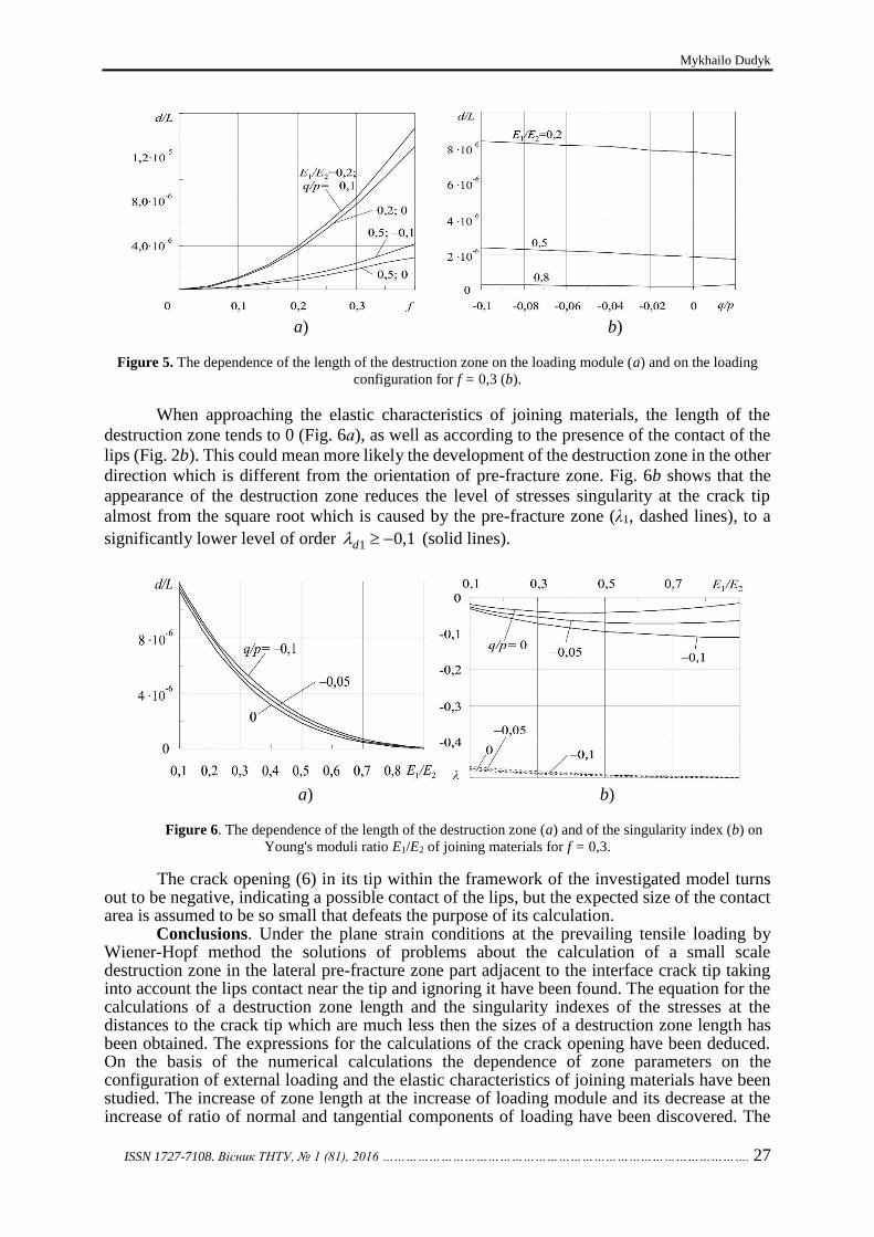
In Fig. 2 the dependence of the length of destruction zone (solid lines) and the sizes of
the area of the contact of the lips (dashed lines) on the loading for comparison are showed. The
length of the destruction zone increases with the increase of dimensionless loading module
(fig. 2а), but it decreases with increasing the ratio of normal and tangential
stresses q/p, which defines the configuration of loading (fig. 2b).
a) b)
Figure 2. The dependence of the lengths of the destruction zone d (solid lines) and the contact area of the lips s
(dashed lines) on the loading module f (a) and on the loading configuration q/p (b).
The analysis of the graphs shows that by ratio of normal and tangential stresses
within the destruction zone is much smaller than the size of the contact area,
which ensures the implementation of the initial condition of the model, whereas under decreasing the contribution in the loading of tangent component q, this condition is violated.
Fig. 3 shows the results of calculations of stresses singularity at different distances to
the tip: if , if and if . As singularity indexes satisfy
inequalities , we can make a conclusion that at distances the level of
stresses concentration is below the square root, but due to the formation of small-scale contact
zone it greatly increases at distances , and the establishment of a destruction zone
eliminates the strengthening of stresses concentration at distances .
Figure 3. The dependence of the singularity indexes of stresses at different distances to the crack tip on the
Young's moduli ratio E1/E2 of joining materials for f = 0,3, q/p = – 0,5.
0y p xy q
2 21/f p q
1 / 0,5q p
d s=
1 s r l= =1 d r s= =
1d r d=
1 1 1d s r l= =
d r s= =
r d=

Mykhailo Dudyk
ISSN 1727-7108. Вісник ТНТУ, № 1 (81), 2016 …………………………………………………………………………………. 25
Taking into account the lateral pre-fracture zone and the contact of the lips the opening
of the crack at its tip will be zero, so that according to deformation criterion the crack start is
impossible [4]. However, the appearance of destruction zones causes the relative shear of crack
lips in its tip, resulting in a shear crack opening δ (4). Fig. 4 shows the dependence of the
normalized shear opening on the magnitude of the external loading at
some of its configuration and some values of Young's modulus ratio of joining materials.
Figure 4. The normalized shear opening of the crack as function of the loading f for q/p = – 0,5 (solid lines) and
q/p = – 1 (dashed lines).
According to the calculations (Fig. 4), the crack opening increases with the magnitude
of the external loading. It behaves like the size of the contact area and the length of the zone of
destruction (Fig. 3): it decreases due to the increasing of normal tensile stress contribution and
due to the approach of the elastic characteristics of joining materials (E1→E2).
2. Computation of the destruction zone ignoring the contact of the lips.
Formulation of the problem and its solution. As it has been established above, with
the significant prevalence in the external loading of tensile efforts in a perpendicular direction
to the crack plane, the length of the contact zone may be smaller then the length of the zone of
destruction and the solution that has been received in the previous part of the article is incorrect.
In this regard, in this part the problem about the destruction zone in the lateral small-scale pre-
fracture zone ignoring the contact of the lips is solved. Assuming the lips of the crack are free
from loading we come to the boundary problem of elasticity which is similar to that one
discussed above with the replacement of conditions in (1) on the lips of the crack with the
conditions
and we formulate the condition at infinity due to the requirement the possibility of sewing
together the wanted solution with the asymptotic solution if in the problem about the
lateral small-scale pre-fracture zone near the tip of the open interfacial crack [8, 9]:
21 1 1/ 4 (1 )E L
: 0,r
0r
1 0
1, , ,i
r i
i
r C C r or
0 1 1
1
2 ( 1), ( ) ( ) / , ( ) ( ) / ,
( 1)
uC u p du p dp D p D p p
D
0,5
1 1
4(1 ) ( 1 ) ( 1 ) ( ) ( 0,5 ) 1 2Re ,
1 2 2( 1 ) ( 1 ) (0,5 ) ( 0,5 )
i
ii i i
i
ki i i
u G F l K iC l
D K i G i
22 1 2 2 1 2 3( ) (1 ) ( ) (1 )(1 ) ( ) ( )(1 ) ( )u p e u p e e u p e e u p
21 4 1 4(1 )( ) ( ) ( ) sin ( ),e e u p e p u p

Destruction Zone Near the Tip of Interfacial Crack at a Prevailing Tensile Loading
26 ……………………………………………………………. .ISSN 1727-7108. Scientific Journal of the TNTU, No 1 (81), 2016
functions , і , the length l of the pre-fracture zone and the angle of its
inclination α are defined in [8, 9]; are the roots of the equation , that satisfy
the condition .
The solution of the formulated problem was received by means of the Wiener-Hopf
method which is similar to the solution of the analogous problem in [7] and leads to the equation
for the determination the length of the zone of destruction d and to the expression for crack
opening δ in its tip:
, (5)
(6)
Analysis of numerical calculations. The numerical analysis of the obtained solution
was made for the same body configuration and loading, as in the previous part of the article,
but considering the ratio of tangential and normal stresses , for which the ignoring
of the contact of the lips is possible. The length of the destruction zone increases with the
increasing of the loading module (Fig. 5а) and decreases with the increasing ratio of tangent
and normal stresses (Fig. 5b). Moreover, its numerical values are of the same order of the length
of the destruction zone which were found with the same parameters of materials and of loading
in the presence of a contact zone in the previous part of the article (Fig. 2b).
21( ) ( 1)sin sin ( 2 ),u p p p p
2 2 22 ( ) sin sin (3 2 ) 2 sin [cos 2 sin ( 2 )u p p p p p p
2sin cos ( )] sin sin ( ),p p p p
2 2 2 23( ) sin sin ( 2 ) 2 sin sin cos ( )] sin sin ( ),u p p p p p p p p
2 2 2 24 ( ) sin sin ( 2 ) 2 sin sin ( )cos sin sin ( ),u p p p p p p p p
2 25( ) sin sin ( );u p p p
( )F 1( )D p ( )G p
i 1( 1 ) 0D x
Re 1i
2 1
0
12
1 0
(1 ) 1
ii i
i i i
C d K JC
K J
1 1 3
2 1
1
ln 4 ( )1( ) exp , ;
2 1 sin
G it t p D pJ x dt G p
x it p D p
2 23 1 31 2 32 33( ) (1 ) sin ( ) ( ) sin [ ( )cos ( )sin ],D p p D p t p p D p p D p p
2 2 231 2 2( ) (1 ) 4(1 )(1 )sin ,D p e e e p 32 1 2( ) (1 ) (1 )sin 2 ,D p e p
233 1 2( ) 2(1 )[ (1 ) 2(1 )]sin ;D p e e p
21 2 1
1 1 2 2 21 2 2
( 1 )2(1 ) ( )sin (1 )(0) ,
( ) sin (1 ) ( )
ii i i
i i i
C d Ked G
E J
1 2 1[ (1 ) (1 ) ]sin ,e
2 2 2 2 2 22 1 1 2 2(1 ) 2(1 ) (1 ) (1 ) ( sin ).e e
| | / 0,1q p
Mykhailo Dudyk
ISSN 1727-7108. Вісник ТНТУ, № 1 (81), 2016 …………………………………………………………………………………. 27
a) b)
Figure 5. The dependence of the length of the destruction zone on the loading module (a) and on the loading
configuration for f = 0,3 (b).
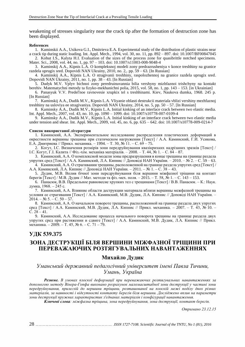
When approaching the elastic characteristics of joining materials, the length of the
destruction zone tends to 0 (Fig. 6а), as well as according to the presence of the contact of the
lips (Fig. 2b). This could mean more likely the development of the destruction zone in the other
direction which is different from the orientation of pre-fracture zone. Fig. 6b shows that the
appearance of the destruction zone reduces the level of stresses singularity at the crack tip
almost from the square root which is caused by the pre-fracture zone (λ1, dashed lines), to a
significantly lower level of order (solid lines).
a) b)
Figure 6. The dependence of the length of the destruction zone (a) and of the singularity index (b) on
Young's moduli ratio E1/E2 of joining materials for f = 0,3.
The crack opening (6) in its tip within the framework of the investigated model turns out to be negative, indicating a possible contact of the lips, but the expected size of the contact area is assumed to be so small that defeats the purpose of its calculation.
Conclusions. Under the plane strain conditions at the prevailing tensile loading by Wiener-Hopf method the solutions of problems about the calculation of a small scale destruction zone in the lateral pre-fracture zone part adjacent to the interface crack tip taking into account the lips contact near the tip and ignoring it have been found. The equation for the calculations of a destruction zone length and the singularity indexes of the stresses at the distances to the crack tip which are much less then the sizes of a destruction zone length has been obtained. The expressions for the calculations of the crack opening have been deduced. On the basis of the numerical calculations the dependence of zone parameters on the configuration of external loading and the elastic characteristics of joining materials have been studied. The increase of zone length at the increase of loading module and its decrease at the increase of ratio of normal and tangential components of loading have been discovered. The
1 0,1d
Destruction Zone Near the Tip of Interfacial Crack at a Prevailing Tensile Loading
28 ……………………………………………………………. .ISSN 1727-7108. Scientific Journal of the TNTU, No 1 (81), 2016
weakening of stresses singularity near the crack tip after the formation of destruction zone has been displayed.
References
1. Kaminskii A.A., Usikova G.I., Dmitrieva E.A. Experimental study of the distribution of plastic strains near a crack tip during static loading. Int. Appl. Mech., 1994, vol. 30, no. 11, pp. 892 – 897. doi: 10.1007/BF00847045
2. Kohut I.S., Kalyta H.I. Evaluation of the sizes of the process zone for quasibrittle notched specimens. Mater. Sci., 2008, vol. 44, no. 1, pp. 97 – 103. doi: 10.1007/s11003-008-9048-4
3. Kaminskij A.A., Kipnis L.A. O kompleksnoj modeli zony predrazrusheniya v konce treshhiny na granice razdela uprugix sred. Dopovidi NAN Ukrainy, 2010, no. 2,. pp. 59 – 63. [In Russian]
4. Kaminskij A.A., Kipnis L.A. O stragivanii treshhiny, raspolozhennoj na granice razdela uprugix sred. Dopovidi NAN Ukrainy, 2011, no. 1, pp. 38 – 43. [In Russian]
5. Dudyk M.V. Vplyv bichnoi zony peredruinuvannia bilia vershyny mizhfaznoi trishchyny na kontakt berehiv. Matematychni metody ta fizyko-mekhanichni polia, 2015, vol. 58, no. 1, pp. 143 – 153. [in Ukrainian]
6. Panasyuk V.V. Predel'noe ravnovesie xrupkix tel s treshhinami. Kiev, Naukova dumka, 1968. 245 p. [In Russian]
7. Kaminskij A.A., Dudik M.V., Kipnis L.A. Vliyanie oblasti destrukcii materiala vblizi vershiny mezhfaznoj treshhiny na usloviya ee stragivaniya. Dopovidi NAN Ukrainy, 2014, no. 5, pp. 50 – 57. [In Russian]
8. Kaminsky A.A., Dudik M.V., Kipnis L.A. Initial kinking of an interface crack between two elastic media. Int. Appl. Mech., 2007, vol. 43, no. 10, pp. 1090 – 1099. doi: 10.1007/s10778-007-0109-4
9. Kaminsky A.A., Dudik M.V., Kipnis L.A. Initial kinking of an interface crack between two elastic media under tension and shear. Int. Appl. Mech., 2009, vol. 45, no. 6, pp. 635 – 642. doi: 10.1007/s10778-009-0214-7 Список використаної літератури
1. Каминский, А.А. Экспериментальное исследование распределения пластических деформаций в окрестности вершины трещины при статическом нагружении [Текст] / А.А. Каминский, Г.И. Усикова, Е.А. Дмитриева // Прикл. механика. – 1994. – Т. 30, № 11. – С. 69 – 75.
2. Когут, І.С. Визначення розмірів зони передруйнування квазікрихких надрізаних зразків [Текст] / І.С. Когут, Г.І. Калита // Фіз.-хім. механіка матеріалів. – 2008. – Т. 44, № 1. – С. 84 – 87.
3. Каминский, А.А. О комплексной модели зоны предразрушения в конце трещины на границе раздела упругих сред [Текст] / А.А. Каминский, Л.А. Кипнис // Доповіді НАН України. – 2010. – № 2. – С. 59 – 63.
4. Каминский, А.А. О страгивании трещины, расположенной на границе раздела упругих сред [Текст] / А.А. Каминский, Л.А. Кипнис // Доповіді НАН України. – 2011. – № 1. – С. 38 – 43.
5. Дудик, М.В. Вплив бічної зони передруйнування біля вершини міжфазної тріщини на контакт берегів [Текст] / М.В. Дудик // Мат. методи та фіз.-мех. поля. – 2015. – Т. 58, № 1. – С. 143 – 153.
6. Панасюк, В.В. Предельное равновесие хрупких тел с трещинами [Текст] / В.В. Панасюк. – К.: Наук. думка, 1968. – 245 с.
7. Каминский, А.А. Влияние области деструкции материала вблизи вершины межфазной трещины на условия ее страгивания [Текст] / А.А. Каминский, М.В. Дудик, Л.А. Кипнис // Доповіді НАН України. – 2014. – № 5. – С. 50 – 57.
8. Каминский, А.А. О начальном повороте трещины, расположенной на границе раздела двух упругих сред [Текст] / А.А. Каминский, М.В. Дудик, Л.А. Кипнис // Прикл. механика. – 2007. – Т. 43, № 10. – С. 28 – 41.
9. Каминский, А.А. Исследование процесса начального поворота трещины на границе раздела двух упругих сред при растяжении и сдвиге [Текст] / А.А. Каминский, М.В. Дудик, Л.А. Кипнис // Прикл. механика. – 2009. – Т. 45, № 6. – С. 71 – 79.
УДК 539.375
ЗОНА ДЕСТРУКЦІЇ БІЛЯ ВЕРШИНИ МІЖФАЗНОЇ ТРІЩИНИ ПРИ ПЕРЕВАЖАЮЧИХ РОЗТЯГУВАЛЬНИХ НАВАНТАЖЕННЯХ
Михайло Дудик
Уманський державний педагогічний університет імені Павла Тичини, Умань, Україна
Резюме. В умовах плоскої деформації при переважаючих розтягувальних навантаженнях за допомогою методу Вінера-Гопфа виконано розрахунок маломасштабної зони деструкції у частині зони передруйнування, прилеглій до вершини тріщини, розташованої на плоскій межі поділу двох різних матеріалів, за наявності і відсутності контакту берегів біля вершини. Досліджено вплив на параметри зони деструкції пружних характеристик з'єднаних матеріалів і конфігурації навантаження.
Ключові слова: міжфазна тріщина, зона передруйнування, зона деструкції, контакт берегів.
Отримано 23.12.15

Вісник Тернопільського національного технічного університету
Scientific Journal of the Ternopil National Technical University
2016, № 1 (81)
ISSN 1727-7108. Web: visnyk.tntu.edu.ua
Corresponding author: Buryk Oleksandr; e-mail: [email protected] …………………………………………………….. 29
UDC 539.3
EVALUATION OF FIRE RESISTANCE OF STRUCTURAL ELEMENTS
CONSIDERING NONLINEARITY OF DEFORMATION PROCESSES
DURING FIRE
Bogdan Drobenko; Aleksander Buryk
Institute of Applied Problems of Mechanics and Mathematics named after
Y.S. Pidstryhach National Academy of Sciences of Ukraine
Summary. A mathematical model for quantitative description of thermomechanical processes in
structural elements under fire was proposed, with taking into account an elastic-plastic deformation and
temperature dependence of material properties. The model is grounded on the equations of heat transfer theory
and nonlinear thermo mechanics and is focused on the numerical methods of research. A method for numerical
simulation of deformation processes in element structures subjected to intensive thermal- power loads was built
on the bases of finite element method. The temperature dependent deformation curves, physical and mechanical
characteristics are approximated by interpolation splines reconstructed by the experimental points of well known
dependencies capturing the mechanical behavior of materials in wide temperature range. As an example, the
computer simulations of thermo mechanical behavior of a steel structure subjected to fire conditions was carried
out. Its fire resistance has been estimated.
Key words: thermo-mechanics, finite element method, fire resistance, the principle of virtual
displacements.
Received 17.02.2016
Problem setting. One of the most important characteristics of building structures is their fire resistance or property to withstand high temperatures during the fire, without losing its load capacity. The majority of works devoted to the study of the properties of structures, has an experimental character. The establishment of modern research programs of fire resistance of structural elements from fires is mainly based on some experiments under conditions of full-scale fires, or a large number of probations and tests in special furnaces, which can withstand ambient temperature according to introduced typical standards [1, 2]. However, opportunities for the study of the behavior of buildings in full-scale fire are rather limited and extremely expensive, and during the experiments in furnaces, as a rule, only some parameters of individual structural elements are taken into consideration often referring to unrealistic size samples, load conditions and destruction. Such experiments do not reflect the behavior of the design as a whole even at low temperatures, as many aspects of the behavior of complex mechanical structures resulting from the interaction of various components cannot be predicted or traced in experiments with isolated elements. Therefore, the actual stresses in real structures during a fire are often substantially lower than anticipated and are based on partial experiments with elements of designs in standard fire scenarios (due to their structural continuity and providing alternative ways of loading individual items).
Due to huge losses during the full-scale experiments and partial nature of the results of experiments in furnaces with individual structural elements a practical need to develop mathematical models with quantitative description and evaluation of fire resistance of structures under different deployment of fire scenarios arises. There is also the necessity to create appropriate software and on this basis to conduct computer modeling of deformation processes of structures under conditions of intense thermal loadings, that meets the requirements of fire.
Analysis of recent researches and publications. In recent years, researches which are dedicated to building of mathematical models predicting fire resistance of elements of building structures, particularly concrete and reinforced concrete buildings have been intensified.

Evaluation of Fire Resistance of Structural Elements Considering Nonlinearity of Deformation Processes During Fire
30 ……………………………………………………………. .ISSN 1727-7108. Scientific Journal of the TNTU, No 1 (81), 2016
Some authors believe that exact model for concrete under conditions of high
temperatures should take into account connectivity process of thermal conductivity, the flow of
viscous liquid, vapor diffusion, capillary effects, and to highlight hidden heat of water phases
variability. Thus series of complex hydro-thermo mechanical models have been proposed
(look, e.g. [3, 4] and other), where moving, temperature, gas pressure, capillary pressure, are
considered to be related. However, due to the complexity of such models, numerical researches
on its basis for the elements for concrete building structures under fire conditions as a rule are
not provided. The basis of simple models are unbound heat equations and the ratio of thermo-
mechanics on the basis of which it is much easier nowadays to conduct computational
experiments and to get adequate results. Transient temperature distributions in structural
elements structures that were defined during the first stage of solving complex tasks are
considered as the input for the second phase of the problem – analysis of stress-strain state of
the construction. There is wide debate concerning the necessity and the methods of
consideration of different factors of influence on the level of development of such models
(look e.g., [5, 6, 7 – 9]).
The purpose of the work is the development of mathematical model, methodology and
software for modeling of deformation processes of structural elements under conditions of
intensive thermal power taking into account loadings, temperature dependence of material
properties and elastic-plastic character of deformation. Availability of reliable software allows
analyzing the behavior of structures during fire, in the process of extinguishing and during
exploitation after fire, to get expert evaluation of fire resistance, stock of resource in the
individual structural elements during the fire, the level of residual stresses after the fire and so
on. This provision provides opportunities for rational choice of geometrical sizes of elements
of constructions, properties of structural and insulating materials with the purpose to continue
the duration of the elements of construction in the midst of the fire with the saving of bearing
capacity. This dramatically reduces the number of field experiments, as only rational projects
are experimentally tested that are obtained through computer simulation.
The formulation of the problem and methods of its solution.
Let’s consider a solid deformable body, which covers area V with the continuous
surface S according to Lipchitz. The body is influenced by the volumetric B
if and surface
S
if forces, given in accordance in the area V and in the part fS of the surface S , of the
movementsS
iu , given on the part uS of the part S ( ufuf SSSSS , ), and also due
to the action of thermal factors caused by the fire. The problem is to determine the stress state
of the body, caused by these influences. In the first phase we form a non-linear non-stationary
problem of thermal conductivity of the body. Environmental temperature change is given in
accordance with the time-temperature curve, which practically defines the scenario of fire
[1, 2].
The temperature field tТ ,r in the body describes the equation
*,0,
tVT
t
Tc r
(1)
under initial
rr 00, TT (2)
and boundary

Bogdan Drobenko, Aleksander Buryk
ISSN 1727-7108. Вісник ТНТУ, № 1 (81), 2016 …………………………………………………………………………………. 31
STТT S rn
(3)
conditions, where r – radius vector of point; Тcc ,r – specific heat; Т,r – density;
T,r – thermal conductivity;
– operator of Hamilton, (
) means the operation of
divergence; n – vector of external single unit to the surface S of the body V ; Т,r –
heat transfer coefficient; ST – environmental temperature. As we can see, thermal
characteristics depend on temperature and on the point which makes it possible to consider
heterogeneous, piecewise and thermo-sensitive bodies.
Since the fire conditions the body is at high temperatures, it can be assumed that the
heat radiation will significantly affect the temperature distribution in the body.
Assuming the generalized heat transfer coefficient as
3223, SSSS TTTTTTÒTÒ , (4)
we can consider that heat transfer between flame and the surface of the body by radiation within
the boundary conditions (3), where – is the index of type of radiation, – constant of
Stefan Boltsman, T та ST – absolute temperatures according to the surface of the body and
the environment (temperature of «pseudo-fire», which rises in accordance with the standards
imposed by fire scenarios), 11/1/1
Sf ( f – emissivity of the flame;
S – absorption capacity of the body surface) [5]. The methodology of solving the problem of
thermal conductivity for thermo-sensitive, piecewise bodies by means of the method of finite
elements of bodies has been proposed and tested in work [10], which presents the results of
solving specific practical problems and the comparative analysis of the numerical solutions with
the results of other authors and relevant experiments has been done.
Unsteady temperature fields that have been defined are the input for the problem of the
second stage which is the determination of the stress-strain state of the body using Lagrange’s
approach, and considering body movement in a fixed Cartesian coordinate system step by step,
when the approximate solution of basic equations, describing equilibrium and compatibility
conditions of the body, is got for discrete moments in time iii ttt 1 , ,1,0i ...
Let’s consider the random next step loading [ t , tt ] (solutions for all previous
discrete moments in time till t including are known).
According to the principle of virtual displacements the body is in equilibrium at the
moment of time tt , if [11]
RVdtt
Vij
tt
ij
tt
0
000 , (5)
where ij
tt
0 , ij
tt
0 – are components of the stress tensor of Piol-Kirchhoff of 2nd type and
deformations of Green-Lagrange that refer to the virtual movements iu imposed on
configuration of the body in the moment of time ttt , which are the functions of Cartesian
coordinates j
ttx
of material point in the moment of time ttt ( j
tt
jj
ttuxx
0);
SdufVdufRtt
S
S
i
S
i
tttt
Vi
B
i
tttt
ftttt
; (6)
Evaluation of Fire Resistance of Structural Elements Considering Nonlinearity of Deformation Processes During Fire
32 ……………………………………………………………. .ISSN 1727-7108. Scientific Journal of the TNTU, No 1 (81), 2016
VVtt
,0
– volume of body according to the moments of time 0t і ttt . Deformations
are determined through movement by using correlation
j
k
t
i
k
t
i
j
t
j
i
t
ij
t
x
u
x
u
x
u
x
u0
0
0
0
0
0
0
0
02
1. (7)
It should be noted that the relationship between the components of Piol-Kirchhoff’s
tensors ij
t0 and Koch’s tensors nm
t (when the forces are related to the unit of the area of the
deformed body) is:
nm
t
n
t
j
m
t
i
tij
t
x
x
x
x
000
0, (8)
where t
,0
– the density of the body in two configurations (when 0t and at the moment of
time t ).
All basic quantities in correlation with (5) are referred to one and the same (initial)
configuration of the body V0 . It gives the opportunity to define the searching movements,
deformations and tenses at the moment of time ttt through the known definitions
ij
t
ij
t
i
tu 000 ,, at the beginning of the proposed step of the loading and the corresponding
increases ijijiu 000 ,, on this stage, that is:
ijij
t
ij
tt
000 ; ijij
t
ij
tt
000 ; ii
t
i
ttuuu 0
. (9)
Taking into consideration the trivial correlation ij
t
ij
tt
ij
000 and presentation
ij
tt
0 and ij
t0 through the movement we get schedule for components
ijijij e 000 , (10)
where linear ( ije0 ) and non-linear ( ij0 ) terms look like:
i
k
j
k
t
j
k
i
k
t
i
j
j
i
ijx
u
x
u
x
u
x
u
x
u
x
ue
0
0
0
0
0
0
0
0
0
0
0
0
02
1 (11)
j
k
i
k
ijx
u
x
u0
0
0
0
02
1
, (12)
Since variation is taken relatively to configuration, corresponding the moment of time
ttt , then 00 ij
t і ijij
tt
00 the original equation of principle of virtual work (1)
taking into account the correlations (9) and (10) looks like:
VdeRVdVdV
ijij
ttt
Vijij
t
Vijij
0
0 00
0
0 00
0
0 00 . (13)

Bogdan Drobenko, Aleksander Buryk
ISSN 1727-7108. Вісник ТНТУ, № 1 (81), 2016 …………………………………………………………………………………. 33
Let’s linearize the resulting equation (13), as we still have a lot of non-linear expressions
in the left part.
Let’s consider approximation to deformation variations ( ijij e00 ) and to
relationships between the stresses and deformations:
)( 0000
T
rsrsijrsij eeC , (14)
where rs
t
ij
t
ijrsC 000 / (the process of constructing a matrix ijrsC0 in the case of non-
isothermal thermo-elastic-plasticity which is described in detail in the monograph [12]); T
rse0 – increases of the temperature deformations in a step of loading. Then:
VdVdeeCV
ijij
t
Vijrsijrs
0
0 00
0
0 000 VdeeCVdeRV
ij
T
rsijrsV
ijij
ttt 0
0 000
0
0 00 . (15)
We are going to write this equation in a convenient matrix-vector form:
V
tT
V
TVdVd
00
0
000
0
000 }{][}{}{][}{ gSgeCe
VdVdRV
T
TV
tTtt 0
000
0
00 00}{][}{}{}{
eCeSe .
(16)
Here tensor components of deformations and stresses are collected in vectors:
Teeeeee )2,2,2,,,(}{ 321312332211e ;
Tgggggg )2,2,2,,,(}{ 321312332211g ;
Tttttttt),,,,,(}{ 2301301203302201100 S .
After substituting the kinematic equations (11) and (12) in (16) we get the linear
approximation for the equations of the motion:
VNL
ttT
NL
tT
VL
tT
L
tTVdVd
00
0
00000
0
00000 }{][}{}{][}{ uBSBuuBCBu
VdeVdRV
TT
L
tT
V
tT
L
tTtt 0
0000
0
000 00}{][}{}{}{
CBuSBu ,
(17)
where T
uuu ),,(}{ 3020100 u – is the vector of increases of movements on the proposed step
of loading, L
tB0 and
NL
tB0 – matrix of differential operators of kinematic equations (11) and
(12) in accordance,
VdVdRS
ST
V
BTtt 0
0
0
0 00}{}{
fufu . (18)
We use the correlation of the principle of virtual works (17) for the definition of the
increases of the movements on the proposed step of loading. It should be noted that its structure
is universal and remains unchanged for all partial cases, in particular, for axisymmetric or plane
problems, and also for the problems which were got due to the usage of assumptions of the
theory of beams and cores. As a result, during the numerical implementation there will be the
only general structure of solution and only the blocks will be changed, that are responsible for

Evaluation of Fire Resistance of Structural Elements Considering Nonlinearity of Deformation Processes During Fire
34 ……………………………………………………………. .ISSN 1727-7108. Scientific Journal of the TNTU, No 1 (81), 2016
calculating the specific characteristics of the matrix-vector L
tB0 ,
NL
tB0 , ][0 C , ][0 S
tetc. For
example, in the case of three-dimensional space problem
T
L
t
xxx
xxx
xxx
2
0
0
3
0
0
3
0
0
1
0
0
3
0
0
2
0
0
1
0
0
2
0
0
1
0
0
0
0 0 0
00 0
00 0
][ B
2
0
0
3
0
30
3
0
0
2
0
30
2
0
0
3
0
20
3
0
0
2
0
20
2
0
0
3
0
10
3
0
0
2
0
10
1
0
0
3
0
30
3
0
0
1
0
30
1
0
0
3
0
20
3
0
0
1
0
20
1
0
0
3
0
10
3
0
0
1
0
10
1
0
0
2
0
30
2
0
0
1
0
30
1
0
0
2
0
20
2
0
0
1
0
20
1
0
0
2
0
10
2
0
0
1
0
10
3
0
0
3
0
30
3
0
0
3
0
20
3
0
0
3
0
10
2
0
0
2
0
30
2
0
0
2
0
20
2
0
0
2
0
10
1
0
0
1
0
30
1
0
0
1
0
20
1
0
0
1
0
10
xx
u
xx
u
xx
u
xx
u
xx
u
xx
u
xx
u
xx
u
xx
u
xx
u
xx
u
xx
u
xx
u
xx
u
xx
u
xx
u
xx
u
xx
u
xx
u
xx
u
xx
u
xx
u
xx
u
xx
u
xx
u
xx
u
xx
u
tttttt
tttttt
tttttt
ttt
ttt
ttt
;
T
NL
t
xxx
xxx
xxx
3
0
0
2
0
0
1
0
0
3
0
0
2
0
0
1
0
0
3
0
0
2
0
0
1
0
0
0
000000
000 000
000000
][ B ;
*0
*0
*0
0
][
S00
0S0
00S
S
t
t
t
t,
330320310
230220210
130120110
*0
ttt
ttt
ttt
tS ,
00 0
00 0
00 0
0 .
For two-dimensional beam of Euler-Bernoulli, which has been got by means of the
introduction of the hypothesis of flat sections [11], whereby movement 21, uu of beam points
define longitudinal movements 1v and hogging 2v of the points of its axis in relations:
)(),(,)(
)(),( 1
0
22
0
1
0
22
1
0
1
0
2
2
2
0
1
0
12
0
1
0
1 xvxxuxd
xvdxxvxxu
( 1x – coordinate along the beam axis), corresponding matrix characteristics have much simpler
form:

Bogdan Drobenko, Aleksander Buryk
ISSN 1727-7108. Вісник ТНТУ, № 1 (81), 2016 …………………………………………………………………………………. 35
2
1
0
2
2
0
1
0
1
0
20
1
0
10
1
00 1xd
dx
xd
d
xd
ud
xd
ud
xd
dtt
L
tB ;
1
0
1
0
0
0
0
xd
d
xd
d
NL
tB ;
11000 }{][ ttt SS .
All integrals in equation are simplified (17), because
1
000
00
xdAdVd
AV
, (19)
where A0 – is a cross-section of the beam.
Because of standard finite-element of sampling area V0 and a certain approximation of
desired increases of nodes movements of every separate element by means of form
function [11] key correlation (17) takes the form
}{}{}]){[]([ FPqKK tt
NLL , (20)
where }{q – is the global vector of the unknown nodes, that allow to determine the increases
movements of body.
We get matrix-vector properties in correlation (20) by means of summing certain
characteristics of specific finite elements: eV
0 :
dve
V
L
tT
L
tTe
L 0
][][][][][][ 000 NBCBNK ;
dve
V
NL
ttT
NL
tTe
NL 0
][][][][][][ 000 NBSBNK ;
le
V
Btt
S
SttTettdvds
00
T][ ][}{ fNfNP
;
dveT
V
t
L
tTe
e
}){][}]({[][}{ 00000
CSBNF . (21)
here ][N – is functions matrix of the form [11], that provides deformation compatibility through
transition from one finite element to another.
Iterative process of the building of nonlinear equations system solving (20) using the
method Newton-Raphson [11] can be represented in three steps.
Step 1. At і – iteration (at the beginning of calculations 1i ) we have initial approach:
for movements )1( ittu , which are defined from finite-element representation
)1()1(}{][
itittqNu (
)0(}{q = u
t ), and deformations )1(
itt
.
Step 2. According to these approximations we calculate )1( itt and then we calculate
tangential matrix of state )1(
0 ][i
C . If there is elastic on the certain step of deformation, then
deformations )1(
itt
give the opportunity to receive voltage directly )1( itt and matrix )1(
0 ][i
C . According to elastic-plastic deformation
)1(
)1(
itt
t
tittd .

Evaluation of Fire Resistance of Structural Elements Considering Nonlinearity of Deformation Processes During Fire
36 ……………………………………………………………. .ISSN 1727-7108. Scientific Journal of the TNTU, No 1 (81), 2016
According to received approach of stresses )1( itt (at the end of )1( i - iteration) we
calculate matrix )1(
0 ][i
C .
Step 3. We form matrix equation:
)1()(}{}{}]){[][(
itttti
NL
tt
L
ttFPqKK
out of which we can define another approach of increases of nodal movements )(
}{i
q on a
certain step of loading, next – approach for the moving of nodes )()1()(
}{}{}{iittitt
qqq
,
movements )(ittu
and deformations )(itt
, after which we go to step 1 of iteration process
(when 1 ii ). Then we continue the calculation on the steps 1 – 3 on the step of loading
[ ttt , ] to achieve convergence.
On the basis of the mathematical model and methodology of solving the formulated
problem of thermal conductivity and thermal elastic-plasticity appropriate software has been
developed.
Methodology of its development is described in detail in the works [12 – 14]. Using
software development thermo-mechanical behavior of a number of steel, concrete and
reinforced concrete structures has been investigated.
As an example of the proposed method we are going to simulate the thermomechanical
behavior of the П-construction, made of heat-sensitive steel С30 under conditions of fire.
The results of computer modeling and analysis.
The dimensions of the construction, terms of its consolidation and power of loading are
shown at the Figure 1.
Figure 1. Steel П-Construction
We consider that out of the inner surface the construction is under the influence of
«pseudo-fire», variable in temperature over time is considered as
)18(10
log3450
tTs
T (21)
according to the international standard ISO 834 [2] (this temperature is taken into account in
the boundary condition) (3) as the temperature of the environment). Other surfaces of the
constructions are isolated.

Bogdan Drobenko, Aleksander Buryk
ISSN 1727-7108. Вісник ТНТУ, № 1 (81), 2016 …………………………………………………………………………………. 37
The dependence of the thermal and mechanical properties of steel from the temperature
is given in the monograph [14]. For approximation of the temperature-dependent deformation
of the curves and physical and mechanical properties of materials the interpolation splines have
been used, which are built according to the points of already known experimental curves that
describes thermo-mechanical behavior of materials in a wide temperature range.
Thermal conductivity problem is solved by means of using isoperimetric quadratic finite
elements [10]. In order to solve thermal elastic-plasticity problem cubic beam finite elements
have been applied [11]. Convergence of the solutions has been investigated by means of
comparison of the numerical solutions on different, according to the density, finite-element
divisions of the construction at various steps of sampling process of thermal conductivity
according to time (when the solutions, that have been got on the certain steps coincide within
1% with the solutions on twice less steps and this convergence was considered to be achieved).
The temperature division in the middle section of the beam cross-bar at the moment of
time, when the construction exhausts its carrying capacity, is shown at Fig. 2.
At Fig. 3 temperature changes of «pseudo-fire» over time are shown TS (curve 1), and
also the temperature on the upper (curve 2) and the lower (curve 3) surfaces of the bar in its
median section of beam which have been in the midst of the fire for two hours.
Analysis of the results shows that during the fire in the beam cross-bar at the beginning
of the sixth minute (t = 320 с) first plastic deformations appear. Ability to elastic-plastic
deformation and further strengthening steel beam is exhausted after 19 minutes. Axial stresses
in the beam at this time are shown at Fig. 4.
Obviously, increasing of the fire resistance of the constructions is connected with the
using of insulation materials from the surface of possible ignition and also with the
manufacturing of the constructions from the materials physical and mechanical properties of
which counteract rapid heating and growth of temperature difference in the construction.
The approach will be used in future for the investigation of thermomechanical behavior
of structures during fire extinguishing and determination of residual stresses in them after a
sharp cooling on the stage of the fire extinguishing that have been launched until the loss of
structure bearing capacity, and also in order to receive expertise review of opportunities for
further exploitation after the fire extinguishing.
Figure 2. Temperature distribution in nodes of the bar middle section at t =19 min.

Evaluation of Fire Resistance of Structural Elements Considering Nonlinearity of Deformation Processes During Fire
38 ……………………………………………………………. .ISSN 1727-7108. Scientific Journal of the TNTU, No 1 (81), 2016
Figure 3. Temperature changes at the bottom (curve 1) and the top (curve 2) surfaces of the bar, and of a
«pseudo-fire» (curve 3).
Figure 4. Stresses at the bottom (curve 1) and the top (curve 2) surfaces of the bar
at moment t = 19 min.
Conclusions. Тhe process of elastic-plastic deformation and temperature dependence
of material properties should be taken into account when modeling thermomechanical processes
in structural elements under the fire. We get the significant deviations in the distributions of
received parameters characterizing stress-strain state structures from actual ones if we do not
consider these factors. It is also important to consider the stage of extinguishing the fire, on
which the residual stresses are actually formed, and evaluate the strength of structures at the
stage of their operation after the fire.
References
1. ASTM Designation: E119. Standard methods of fire test of building construction and materials.
Philadelphia, USA, PA: American Society for Testing and Materials, 1983.
2. International Organization for Standardization. Fire resistance test on elements of building construction.
ISO, 834, Geneva, Switzerland, 1975.
3. Gawin D, Majorana C, Pesavanto F, Schrefler B.A fully coupling multiphase model of higro-thermo-
mechanical behavior of concrete at high temperature. In: Computational mechanics, new trends and applications,
Barcelona, Spain: CIMNE, 1998, pp. 1 – 19.

Bogdan Drobenko, Aleksander Buryk
ISSN 1727-7108. Вісник ТНТУ, № 1 (81), 2016 …………………………………………………………………………………. 39
4. Mounajed G, Obeid W. A new coupling F.E. model for the simulation of thermal hydro-mechanical
behavior of concrete at high temperatures. Mater. Struct., 2004, vol. 37, pp. 422 – 432.
5. Chung K., Park S., Choi S. Material effect for predicting the fire resistance of concrete-filled square steel
tube column under constant axial load. Journal of Constructional Steel Research, 2008, vol. 64, no. 12, pp. 1505 –
1515.
6. Haksever A., Anderberg Y. Comparison between measured and computed structural response of some
reinforced concrete columns in fire. Fire Safety Journal, 1981, no. 4, pp. 293 – 297.
7. Huang Z., Platten A. Non-linear finite element analysis of planar reinforced concrete members subjected
to fires. ACI Struct. J., 1997, vol. 94, no. 3, pp. 272 – 282.
8. Huang Z., Platten A., Roberts J. Non-linear finite element model to predict temperature histories within
reinforced concrete in fires. Build Environ., 1996, vol. 31, no. 2, pp. 109 – 118.
9. Huang Z.-F., Tan K.-H., Fire resistance of compartments within a high-rise steel frame: New sub-frame
and isolated member models. Journal of Constructional Steel Research, 2006, vol. 62, pp. 974 – 986.
10. Drobenko B., Buryk O. To the estimation of temperature fields in building structures subjected to the fire.
Mechanical engineering, 2013, no. 5 – 6, pp. 16 – 20. [in Ukrainian]
11. Bathe, K.J. Finite Element Procedures Analysis. Englewood Cliffs: Prentice Hall, New Jersey, 1995.
1037 p.
12. Hachkevych О.R., Drobenko B.D. Special features of numerical analysis of coupled electromagnetic,
thermal and mechanical fields in thermo-sensitive electro-conductive solids subjected to quasi-steady
electromagnetic loadings, Mat. Metody and Fiz.-Mekh. Polya, 2007, vol. 50, no. 3, pp. 166 – 177. [in Ukrainian]
13. Drobenko B., Hachkevych A., Kournyts’kyi T. Thermomechanical behaviour of polarizable and
magnetizable electroconductive solids subjectted to induction heating, Journal of Engineering Mathematics, 2008,
vol. 61, no. 2 – 4, pp. 249 – 269.
14. Modeling and optimization In thermomechanics of electroconductive heterogeneous solids. Edited by
Ya.J. Burak and R.M. Kushnir. Vol. 4: Thermomechanics of magnetizable electroconductive thermosensitive
solids, O.R. Hachkevych, B.D. Drobenko, Lviv: SPOLOM, 2010. 256 p. [in Ukrainian]
Список використаної літератури
1. ASTM Designation: E119. Standard methods of fire test of building construction and materials.
Philadelphia, PA: American Society for Testing and Materials; 1983.
2. International Organization for Standardization. Fire resistance test on elements of building construction.
ISO/834, 1975.
3. Gawin D, Majorana C, Pesavanto F, Schrefler B. A fully coupling multiphase model of higro-thermo-
mechanical behavior of concrete at high temperature. In: Computational mechanics, new trends and applications. –
Barcelona, Spain: CIMNE. – 1998. – P. 1 – 19.
4. Mounajed G, Obeid W. A new coupling F.E. model for the simulation of thermal hydro-mechanical
behavior of concrete at high temperatures // Mater. Struct. – 2004. – 37. – P. 422 – 432.
5. Chung K., Park S., Choi S. Material effect for predicting the fire resistance of concrete-filled square steel
tube column under constant axial load // Journal of Constructional Steel Research. – 2008. – 64, № 12. – P. 1505 –
1515.
6. Haksever A., Anderberg Y. Comparison between measured and computed structural response of some
reinforced concrete columns in fire // Fire Safety Journal. – 1981. – 4. – P. 293 – 297.
7. Huang Z., Platten A. Non-linear finite element analysis of planar reinforced concrete members subjected
to fires // ACI Struct. J. – 1997. – 94, № 3. – P. 272 – 282.
8. Huang Z., Platten A., Roberts J. Non-linear finite element model to predict temperature histories within
reinforced concrete in fires // Build Environ. – 1996. – 31, № 2. – P. 109 – 118.
9. Huang Z.-F., Tan K.-H., Fire resistance of compartments within a high-rise steel frame: New sub-frame
and isolated member models // Journal of Constructional Steel Research. – 2006. – 62. – P. 974 – 986.
10. Дробенко, Б. До оцінювання температурних полів в елементах будівельних конструкцій за умов
пожежі [Текст] / Б. Дробенко, О. Бурик // Машинознавство. – 2013. – № 5 – 6. – С. 16 – 20.
11. Bathe, K.J. Finite Element Procedures Analysis. – Englewood Cliffs: Prentice Hall, 1995. – 1037 p.
12. Гачкевич, О.Р. Особливості числового розв’язування зв’язних задач про визначення
електромагнітних, теплових і механічних полів у деформівних термочутливих електропровідних тілах за
Evaluation of Fire Resistance of Structural Elements Considering Nonlinearity of Deformation Processes During Fire
40 ……………………………………………………………. .ISSN 1727-7108. Scientific Journal of the TNTU, No 1 (81), 2016
квазіусталених електромагнітних навантажень [Текст] / О.Р. Гачкевич, Б.Д. Дробенко // Мат. методи і
фіз.-мех. поля. – 2007. – 50, № 3. – С. 166 – 177.
13. Моделювання та оптимізація в термомеханіці електропровідних неоднорідних тіл; за заг. ред.
Я.Й. Бурака, Р.М. Кушніра. Т. 4: Термомеханіка намагнечуваних електропровідних термочутливих тіл
[Текст] / О.Р. Гачкевич, Б.Д. Дробенко. – Львів: СПОЛОМ, 2010. – 256 с.
14. Drobenko B., Hachkevych A., Kournyts’kyi T. Thermomechanical behaviour of polarizable and
magnetizable electroconductive solids subjectted to induction heating/ Journal of Engineering Mathematics. –
2008. – 61, № 2 – 4. – P. 249 – 269.
УДК 539.3
ОЦІНЮВАННЯ ВОГНЕТРИВКОСТІ ЕЛЕМЕНТІВ КОНСТРУКЦІЙ
З УРАХУВАННЯМ НЕЛІНІЙНОСТІ ПРОЦЕСІВ ЇХ
ДЕФОРМУВАННЯ
Богдан Дробенко; Олександр Бурик
Інститут прикладних проблем механіки і математики
ім. Я.С. Підстригача НАН України, Львів, Україна
Резюме. Запропоновано орієнтовану на використання числових методів дослідження
математичну модель кількісного опису термомеханічних процесів в елементах конструкцій під час
пожежі з урахуванням пружно-пластичного характеру деформування та температурної залежності
фізико-механічних характеристик матеріалів. Модель базується на залежностях теорії
теплопровідності та нелінійної термомеханіки. Побудовано з використанням методу скінченних
елементів методику чисельного моделювання процесів деформування конструкцій за інтенсивних
температурних та силових навантажень. Для апроксимації температурно-залежних кривих
деформування та фізико-механічних характеристик матеріалів використано інтерполяційні сплайни,
побудовані за точками відомих експериментальних кривих. Як приклад, виконано комп’ютерне
моделювання термомеханічної поведінки сталевої конструкції за умов пожежі. Отримано оцінку її
вогнетривкості.
Ключові слова: термомеханіка, метод скінченних елементів, вогнетривкість, принцип
віртуальних переміщень.
Отримано 17.02.2016

Вісник Тернопільського національного технічного університету
Scientific Journal of the Ternopil National Technical University
2016, № 1 (81)
ISSN 1727-7108. Web: visnyk.tntu.edu.ua
Corresponding author: Grigoryeva Ludmila; e-mail: [email protected] ………………………………………………….. 41
UDC 534-21: 537.226.86
RESONANCE RADIAL OSCILLATIONS OF A PIEZOCERAMIC
CYLINDERS AND SPHERES TAKING INTO ACCOUNT
ELECTROMECHANICAL LOSSES
Oleksandr Bezverhyi1; Ludmila Grigoryeva2; Sergiy Grigoryev3
1,2 S. P. Tymoshenko Institute of Mechanics of NAS of Ukraine, Kyiv, Ukraine
3 Kyiv National University of Building and Architecture, Kyiv, Ukraine
Summary. Hollow piezoceramic radially polarized cylinders and spheres widely used as sound
transducers and receivers are considered. The most characteristic run mode of piezoceramic transmitters is
resonant mode. In this paper, a universal approach to solving of problems of forced thickness oscillations of
piezoceramic cylinders and spheres is expanded on research of amplitude of the electromechanical state with due
regard to mechanical, dielectric, piezoelectric energy losses. General equation system of steady oscillation of
cylinders and spheres is reduced to Hamiltonian equation system which is solved by superposition of solutions of
initial problems. The suggested approach enables to research into oscillation of the transmitters under electrical
and mechanical load and arbitrary boundary conditions. For calculation of electromechanical state of
transmitters at resonance modes the energy dissipation counts towards by the introduction of complex physical
constants with predetermined values of tangents of losses. The oscillations of spheres and cylinders with electrode
free outer surfaces under loading by electric potential difference are studied. The amplitude of movement of the
outer surface depending on the loading frequency and geometrical dimension of the figures is considered. The
amplitude of movement in the neighbourhood of the first resonance at different values of tangents of losses is
studied; oscillations forms on the first three resonances are built.
Key words: piezoceramic transmitters, radially polarized cylinder and sphere, forced oscillations, energy
losses, tangents of losses, resonance frequencies.
Received 01.03.16
Introduction. Piezoceramic radially polarized cylinders and spheres are widely used in
different scientific and technical fields as sound transducers and receivers, which operate at
wide frequency range [1 – 4]. The most characteristic run mode of piezoceramic transmitters
is resonant mode [5]. Fixed oscillations of piezoceramic layers with curved surfaces have been
investigated in works [6, 7]. Propagation of oscillations in magneto-electro-elastic hollow
cylinders have been studied in work [8]. Free oscillations of piezoceramic hollow sphere have
been examined in work [9].
To calculate electromechanical condition of piezoceramic transmitters at resonance run
modes dissipation of material energy introducing complex material coefficients [1 – 3] with
specific meanings of tangents of losses should be taken into account. Experimental
determinative methods of real and imaginary complex material constants have been described
in works [10 – 13]. Investigations are done on series of samples of different forms and direction
of polarization. Considerable material, experimental and mathematical base is necessary for
finding nine unknown tangents of losses. Results depend on mode of load, conditions of
production and operation of a sample, operating temperature, quality factor, which may differ
at resonance and anti-resonance in several times.
§1. Problem statement. The influence of viscoelastic characteristics on radial
oscillations of polarized in thickness cylinders and spheres at loading by difference of potentials
was investigated. Coordinate is changed within , where − radius
of middle surface, − thickness of wall. Oscillations of body in general case are described
by equations of movement [4]
)(2 tV r hRrhR R
h2

Resonance radial oscillations of a piezoceramic cylinders and spheres taking into account electromechanical losses
42 ……………………………………………………………. .ISSN 1727-7108. Scientific Journal of the TNTU, No 1 (81), 2016
, (1.1)
quasi-static equation of Maxwell for electric variables
, (1.2)
which are added by material relations at radial polarization
;
;
. (1.3)
At equations (1.1), (1.2) are correspond to cylindrical coordinates, at
− spherical system of coordinates. The given scheme at gives also denouement
about oscillations of thickness of piezoceramic layer.
Energy dissipation can be taken into consideration introducing complex material
constants in physical correlation [3-5] (1.3) in mono-harmonic approaching within viscoelastic
model. Complex modules are introduced by following correlations:
, , , (1.4)
where , , – tangents of angles of mechanical, dielectric and piezoelectric losses.
Energy dissipation influence is the most noticeable at resonance run modes owing to
smallness of loss tangents. Thus, to compare forced oscillations of transmitters taking into
account energy dissipation and without it and investigate oscillations of piezoceramic bodies at
resonance frequencies is our aim. Because of difficulty of defining full set of material
characteristics together with loss tangents, we will consider the case when tangents of
mechanic, dielectric and piezoelectric losses are equal and occur in the range from 0.5% to 2%.
Forced oscillations of cylinders and spheres. Harmonic oscillations
, arising at load of piezo-element owing to difference of electric
potential , applied to electroded outer surfaces is going to be considered.
Approach, suggested in works [6, 7] will be used to investigate forced oscillations. By
transformation of dependences (1.1) (1.2) together with (1.3), operating system of Hamiltonian
equations along spatial coordinate for amplitude meanings of parameters of electromechanical
state is got
a
r
Na
rr
Na
rr
N
Drr
Ner
r
N
c
c
r
r
*33
*31
*33
*13
a
r
Nucc
Nc
c
cc
ee
r
Nr
121111
*33
*13
13
*33
*13
132
2
2
2
1
,
2
2
)(t
u
r
N
rrr
rr
0
r
DN
r
D rr
re
r
uNc
r
ucrr
331333
re
r
uccNcN
r
uc
3123111113 )])(1(
2
1[
rr
uNe
r
ueDr
333133
1N
2N 0N
)1( ij
E
ijij cicc
)1( ijijij eiee
)1( ij
S
ijij i
ijc ije ij
tirftrfa expRe,
tiV exp2Re 0

Oleksandr Bezverhyi, Ludmila Grigoryeva, Sergiy Grigoryev
ISSN 1727-7108. Вісник ТНТУ, № 1 (81), 2016 …………………………………………………………………………………. 43
,
,
(2.1)
according to functions , , , . Signs are used here
, , 33
3313
13*13c
ecee , .
System (2.1) can be reduced to Hamilton equation system introducing chosen canonic
variables and characteristic function of Hamilton.
For equation system (2.1), boundary conditions are put on surfaces і
using one of alternative couples
,
. (2.2)
When needed, limit conditions of impedance (mixed) type can be established.
Further denouement can be searched as a vector
. (2.3)
Equation system of electric elasticity (2.1) and conditions (2.2) are reduced to non-
dimensional form
, , , , ,
, , , ,
, , , ,
. (2.4)
0
r
Dra
r
N
a
r
a
r
N
N
a
rr
N
N
a
r urc
NcDr
rc
er
rcr
u
*33
*31
*3333
33
*33
1
a
r
a
r
N
N
a
rr
N
N
a
ur
NeDr
rc
cr
rc
e
r *33
*31
*3333
33
*3333
33
rr
Nr r
NDr
ru
33
3313
13*13
eecc
33
3333
33*33
eecc
33
3333
33*33c
ee
hRr 0
hRr 1
tutruttr rrrrrr
0
0
0
0 ,,
tutruttr rrrrrr
1
1
1
1 ,,
),,,( 4321 YYYYY ),,,(aa
r
a
r
Na
rr
NuDrr
xRr h
xx
ht
tt
h
uu
00c
σσ rr
rr
00c
00
00
ch
0000c
DD r
r 00
00
ch
00
00c
cc
ijij
0000c
ee
ijij
00
3333
R
h

Resonance radial oscillations of a piezoceramic cylinders and spheres taking into account electromechanical losses
44 ……………………………………………………………. .ISSN 1727-7108. Scientific Journal of the TNTU, No 1 (81), 2016
where , , , . Here − parameter of curvature. Taken
non-dimension allows to transfer from spatial coordinate to non-dimensional coordinate
, . Further signs of non-dimension are omitted.
System (2.1) in non-dimensional form is of the following form
,
,
,
. (2.5)
Amplitude of oscillations of electrical potential on outer surfaces is known
(2.6)
Let mechanic load of outer surfaces be absent
. (2.7)
To do boundary value problem (2.5) – (2.7), generally accepted problem-solving
methods (discrete orthogonalization method, collocation method, superposition of denouement
of initial problems [6, 7]) can be used.
Oscillations of radial polarized bodies of ceramic PZT-4 with following material
parameters are examined:
, ,
, , ,
, , .
00E
cc 3300 S3300 E
h cht 33
r
x 11 x
2
*33
*31
1
*33
*131
11Y
x
NeY
x
N
c
c
x
Y
3121111
*33
*13
13
*33
*13
132
22
2
2
1
)1(
1Ycc
Nc
c
cc
ee
x
NxN
02
x
Y
3
*33
*31
2
*3333
33
1
*33
3
1)1()1(Y
x
N
c
cY
xc
eY
xcx
YN
N
N
N
3
*33
*31
2
*3333
33
1
*3333
334
1)1()1(Y
x
NeY
xc
cY
xc
e
x
YNN
0)( VhRa
04 )1( VY
0)( hRrr
a 0)1(1 Y
210
11 /109,13 мНcE
210
12 /1078,7 мНcE
210
13 /1043,7 мНcE
210
33 /105,11 мНcE
2
31 /2,5 мКлe
2
33 /1,15 мКлe мФS
/1056211
33
3
/7500 мкг
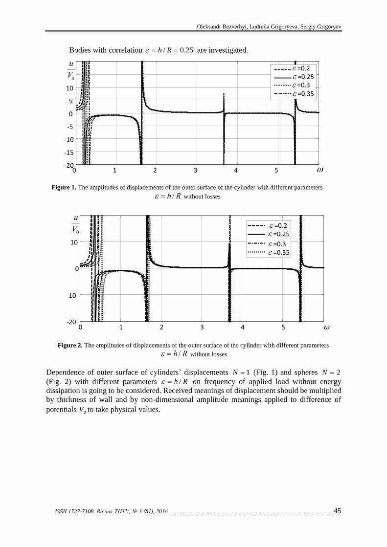
Oleksandr Bezverhyi, Ludmila Grigoryeva, Sergiy Grigoryev
ISSN 1727-7108. Вісник ТНТУ, № 1 (81), 2016 …………………………………………………………………………………. 45
Bodies with correlation are investigated.
Dependence of outer surface of cylinders’ displacements (Fig. 1) and spheres
(Fig. 2) with different parameters on frequency of applied load without energy
dissipation is going to be considered. Received meanings of displacement should be multiplied
by thickness of wall and by non-dimensional amplitude meanings applied to difference of
potentials to take physical values.
25.0/ Rh
1N 2N
Rh /
0V
0 1 2 3 4 5 -20
-15
-10
-5
0
5
10
=0.2 =0.25 =0.3 =0.35
Figure 1. The amplitudes of displacements of the outer surface of the cylinder with different parameters
without losses
0 1 2 3 4 5 -20
-10
0
10
=0.2 =0.25
=0.3 =0.35
Figure 2. The amplitudes of displacements of the outer surface of the cylinder with different parameters
without losses

Resonance radial oscillations of a piezoceramic cylinders and spheres taking into account electromechanical losses
46 ……………………………………………………………. .ISSN 1727-7108. Scientific Journal of the TNTU, No 1 (81), 2016
Interval of frequency change involves first four own frequencies. Amplitude of
displacements on resonances takes theoretically unlimited meanings. Higher resonances for
different bodies are close to each other, the most difference is observed at first resonance. At
decreasing the first resonance approaches to zero. There are following resonance frequencies
at 25.0 : for cylinder , for sphere .
Detailed curves of modules of the amplitude of displacements taking into account
energy dissipation with different tangents meanings of losses were shown in
Fig. 3 and Fig. 4. Distinct dependence between the amplitude of oscillations and tangents of
losses is observed. Dependence nonlinearity is more observable for sphere.
)662.3,627.1,235.0( )677.3,651.1,381.0(
ijc ije cij
0.2 0.22 0.24 0.26 0
50
100
150
200
250
c=0.005
c=0.01
c=0.015
c=0.02
Figure 3. Modules of the amplitude of
displacements of the cylinder near
the first resonance at different values of loss
tangents
0.35 0.36 0.37 0.38 0.39 0.4 0
50
100
150
200
250
c=0.005
c=0.001 c=0.015 c=0.02
Figure 4. Modules of the amplitude of
displacements of the sphere near
the first resonance at different values of loss
tangents
-1 -0.5 0 0.5 х -1.5
-1
-0.5
0
0.5
1
и
=0.23
=1.627
=3.661 -1 -0.5 0 0.5 х
-2
-1.5
-1
-0.5
0
0.5
1
1.5
и
=0.377 =1.65 =3.678
Figure 5. The first three forms of cylinder
vibration ( )
Figure 6. The first three forms of sphere
vibration ( )

Oleksandr Bezverhyi, Ludmila Grigoryeva, Sergiy Grigoryev
ISSN 1727-7108. Вісник ТНТУ, № 1 (81), 2016 …………………………………………………………………………………. 47
Oscillation forms at first three resonances are shown in Fig. 5, 6. Displacement
correlations of body points to the amplitude of oscillations of outer surface were illustrated in
these figures.
Conclusions. Suggested generalized approach to solving of problems of radial
oscillations of piezoceramic cylinders and spheres gives opportunity to effectively investigate
forced oscillations of piezoceramic bodies with different geometrical parameters, define
resonance frequencies, investigate dependence of the amplitude of parameters of
electromechanical state on tangents of losses.
References
1. Karnauxov V.G. Nelinejnaya termomexanika p'ezoe'lektricheskix neuprugix tel pri monogarmonicheskom
nagruzhenii / Karnauxov V.G., Mixajlenko V.V. – Zhitomir: ZhGTU, 2005. – 428 s.
2. Mason, W. Piezoelectric crystals and their applications to ultrasonics. – Van Nostrand, New York. – 1950. –
448 с.
3. Parton V.Z. E'lektromagnitouprugost' p'ezoe'lektricheskix i e'lektroprovodnyx tel / Parton V.Z.,
Kudryavcev B.A. – M.: Nauka, 1988. – 472 s.
4. Shul'ga N.A. Kolebaniya p'ezokeramicheskix tel / Shul'ga N.A., Bolkisev A.M. – K.: Naukova dumka,
1990. – 228 s.
5. Shul'ha M.O. Rezonansni elektromekhanichni kolyvannya p’yezoelektrychnykh plastyn / Shul'ha M.O.,
Karlash V.L. – K.: Naukova dumka, 2007. – 186 s.
6. Shul'ga N.A. Comparative Analysis of the Electroelastic Thickness Vibrations of Layers with Curved
Boundaries / Shul'ga N.A., Grigor'eva L.O. // Int. Appl. Mech. – 2011. – 47, N 2. – P. 177 – 185.
7. Shulga M.O. Electromechanical unstationary thickness vibrations of piezoceramic transformers at electric
excitation / Shulga M.O., Grigoryeva L.O. // Mechanical Vibrations: Types, Testing and Analysis. − Nova Science
Publishers, New York. − 2011. − Р. 179 – 204.
8. J. Yu. Wave propagation in non-homogeneous magneto-electro-elastic hollow cylinders / J. Yu, Q. Ma,
Sh. Su. // Ultrasonics. – Volume 48, Issue 8, December 2008, Pages 664 – 677.
9. V. Chiroiu. On the free vibrations of a piezoceramic hollow sphere / V. Chiroiu, L. Munteanu // Mechanics
Research Communications. Volume 34, Issue 2, March 2007, Pages 123 – 129.
10. Bolkisev A.M. Dissipaciya e'nergii pri garmonicheskom nagruzhenii vyazkouprugogo
p'ezokeramicheskogo materiala / Prikl. mexanika. – 1987. – 23, № 3. – S. 48 – 53.
11. Karlash V.L. Shche raz pro vtraty enerhiyi v p"yezokeramichnykh rezonatorakh // Akust. visnyk. – 2015. –
T. 17, № 1. – S. 34 – 47.
12. S. Sherrit. Non-iterative Evaluation of the Real and Imaginary Material Constants of Piezoelectric
Resonators / S. Sherrit, H.D. Wiederick, B.K. Mukherjee // Ferroelectric, 1992, Vol. 134, pp. 111 – 119.
13. Uchino K. Loss Determination Metodology for a Piezoelectrical Theory and Experimental Proposals /
Uchino K., Zhuang Y., O. Ural S. // J. of Advanced Dielectrics. Vol. 1, No. 1. – 2011. – P. 17 – 31.
Список використаної літератури
1. Карнаухов, В.Г. Нелинейная термомеханика пьезоэлектрических неупругих тел при
моногармоническом нагружении [Текст] / Карнаухов В.Г., Михайленко В.В. – Житомир: ЖГТУ, 2005. –
428 с.
2. Мэзон, У. Пьезоэлектрические кристаллы и их применения в ультраакустике [Текст] /
Мэзон У. – М.: Изд-во иностр. лит., 1952. – 448 с.
3. Партон, В.З. Электромагнитоупругость пьезоэлектрических и электропроводных тел [Текст] /
Партон В.З., Кудрявцев Б.А. – М.: Наука, 1988. – 472 с.
4. Шульга, Н.А. Колебания пьезокерамических тел [Текст] / Шульга Н.А., Болкисев А.М. – К.: Наукова
думка, 1990. – 228 с.
5. Шульга, М.О. Резонансні електромеханічні коливання п’єзоелектричних пластин [Текст] /
Шульга М.О., Карлаш В.Л. – К.: Наукова думка, 2007. – 186 с.
6. Shul'ga N.A. Comparative Analysis of the Electroelastic Thickness Vibrations of Layers with Curved
Boundaries / Shul'ga N.A., Grigor'eva L.O. // Int. Appl. Mech. – 2011. – 47, N 2. – P. 177 – 185.

Resonance radial oscillations of a piezoceramic cylinders and spheres taking into account electromechanical losses
48 ……………………………………………………………. .ISSN 1727-7108. Scientific Journal of the TNTU, No 1 (81), 2016
7. Shulga M.O. Electromechanical unstationary thickness vibrations of piezoceramic transformers at electric
excitation / Shulga M.O., Grigoryeva L.O. // Mechanical Vibrations: Types, Testing and Analysis. − Nova Science
Publishers, New York. − 2011. − Р. 179 – 204.
8. J. Yu. Wave propagation in non-homogeneous magneto-electro-elastic hollow cylinders / J. Yu, Q. Ma,
Sh. Su. // Ultrasonics. – Volume 48, Issue 8, December 2008, Pages 664 – 677.
9. V. Chiroiu. On the free vibrations of a piezoceramic hollow sphere / V. Chiroiu, L. Munteanu // Mechanics
Research Communications. Volume 34, Issue 2, March 2007, Pages 123 – 129.
10. Болкисев, А.М. Диссипация энергии при гармоническом нагружении вязкоупругого
пьезокерамического материала [Текст] / А.М. Болкисев // Прикл. механика. – 1987. – Т. 23, № 3. – С. 48 –
53.
11. Карлаш, В.Л. Ще раз про втрати енергії в п’єзокерамічних резонаторах [Текст] / В.Л. Карлаш //
Акуст. вісник. – 2015. – Т. 17, № 1. – С. 34 – 47.
12. S. Sherrit. Non-iterative Evaluation of the Real and Imaginary Material Constants of Piezoelectric
Resonators / S. Sherrit, H.D. Wiederick, B.K. Mukherjee // Ferroelectric, 1992, Vol. 134, pp. 111 – 119.
13. Uchino K. Loss Determination Metodology for a Piezoelectrical Theory and Experimental Proposals /
Uchino K., Zhuang Y., O. Ural S. // J. of Advanced Dielectrics. Vol. 1, No. 1. – 2011. – P. 17 – 31.
УДК 534-21:537.226.86
РЕЗОНАНСНІ РАДІАЛЬНІ КОЛИВАННЯ П’ЄЗОКЕРАМІЧНИХ
ЦИЛІНДРІВ ТА КУЛЬ
З УРАХУВАННЯМ ЕЛЕКТРОМЕХАНІЧНИХ ВТРАТ
Олександр Безверхий1; Людмила Григор’єва2; Сергій Григор’єв3
1,2Інститут механіки ім. С.П. Тимошенка НАН України, Київ, Україна 3Київський національний університет будівництва і архітектури,
Київ, Україна
Резюме. Поширено універсальний підхід до розв’язання задач про вимушені товщинні коливання
п’єзокерамічних циліндрів та куль на дослідження амплітудних значень електромеханічного стану в околі
резонансних частот із урахуванням механічних, діелектричних, п’єзоелектричних втрат енергії.
Розглянуто амплітудні значення переміщень зовнішньої поверхні залежно від частоти навантаження та
геометричних розмірів тіл, досліджено амплітудні значення переміщень в околі першого резонансу при
різних значеннях тангенсів втрат, побудовано форми коливань на перших трьох резонансах.
Ключові слова: п’єзокерамічні перетворювачі, радіально поляризований циліндр та куля,
вимушені коливання, втрати енергії, тангенси втрат, резонансні частоти.
Отримано 01.03.16

Вісник Тернопільського національного технічного університету
Scientific Journal of the Ternopil National Technical University
2016, № 1 (81)
ISSN 1727-7108. Web: visnyk.tntu.edu.ua
Corresponding author: Dubyk Iaroslav; e-mail: [email protected] …………………………………………………………………… 49
UDC 539.4
FLUID-STRUCTURE INTERACTION IN FREE VIBRATION
ANALYSIS OF PIPELINES
Iaroslav Dubyk; Igor Orynyak
G.S. Pisarenko Institute for Problems of Strength, National Academy of Sciences
of Ukraine, 2 Tymiryazevs’ka str., Kyiv, Ukraine
Summary. We analyze the impact of the transported fluid on the natural frequencies of a pipeline. Solution of coupled acousto-mechanical problem for straight pipe is given by the Transfer Matrix Method. The equations for junction coupling are given. Several practical examples demonstrate the importance of taking into account the fluid-structure interaction. It is shown that treating fluid as an added mass at the axial vibrations can lead to significant errors.
Key words: pipeline, acousto-mechanical vibration, natural frequency Received 10.03.2016
Introduction. The presence of the fluid in the pipe affect the dynamic behavior of the considered system. In its simplest form, one can take into account the fluid as an added mass, but this approach can lead to significant errors, especially in the calculation of dynamic events such as a water hammer. In a more detailed analysis is necessary to consider the interaction that occurs between the pipe and the fluid. The interaction between the internal fluid (liquid or gas) and the pipeline is performed by superimposing of the four mechanisms [1 – 3]:
Fitting coupling;
Poisson coupling;
Friction coupling;
Burdon coupling. The interaction may be strong or bilateral, and unilateral or weak. One-way interaction
is a classical scheme, at the beginning the speed and pressure in the fluid are calculated, and then these values as external loads are applied to the pipeline. Calculation scheme of bilateral interaction is more complicated, but allows you to get the correct dynamic response of the system.
The main effects of fluid-structure interaction are problem dependent [1]. When compared to predictions of conventional water hammer and uncoupled analyses, predictions including fluid-structure interaction may lead to: higher or lower extreme pressures and stresses, changes in the natural frequencies of the system, and more damping and dispersion in the pressure and stress histories. Fully coupled analysis is required in the calculation of compliant structures, which are subject to sudden loads. Generally speaking, coupled analysis gives more accurate results in the calculation pressures, stresses and displacements, and its own resonance frequency and damping forces in the supports.
The natural frequencies of the pipeline are usually obtained by taking into account the fluid as an added mass. The natural frequencies of the fluid, if necessary, get on the assumption of the rigid walls. This approach will give wrong results in systems where the natural frequencies of the pipeline and the fluid are close to each other. A coupled analysis of the interaction on the fittings (i.e. pipe bends) will lead to a separation of coincident natural frequencies [1, 4]. Thus, the coupling accounting prevents resonance, which is obtained by the uncoupled analysis.
Despite the practical importance and numerous studies [1, 5], the calculation scheme of coupled FSI is in the area of academic interest and almost has no use in practice. It is due to several factors:

Fluid-Structure Interaction in free vibration analysis of pipelines
50 ……………………………………………………………. .ISSN 1727-7108. Scientific Journal of the TNTU, No 1 (81), 2016
The solution of separate problems by numerical methods. These solutions are aimed
to show the presence of the coupling effect and do not offer a universal algorithm for solving
the entire class of similar problems. Such solutions are cumbersome and are hardly
programmed, their practical application is limited.
Pipeline software packages (ASTRA, CAESAR) do not have the possibility of
coupled analysis, fluid is accounted as an added mass;
Universal FEM computer codes (ANSYS, ABAQUS), can solve the problems of
coupled FSI only in three-dimensional form, that is expensive and impractical in the calculation
of piping systems.
Show practicability of coupled acousto-mechanical calculations in the analysis of piping
vibration is the main goal of this work. To solve this purpose it is necessary to address the
following tasks:
Summarize the work on the analysis of the FSI for complex systems;
Demonstrate the practical application of the proposed analysis algorithm and show
the importance of considering FSI.
At the beginning the brief derivation of the basic equations is given, in more detail it
can be found elsewhere [2, 3]. Then, the search algorithm of the natural frequencies is
presented, and in the second part a few practical examples are considered.
Mathematical equations for the straight pipe. Set of the Skalak equations for the
straight pipe run:
FE
txN
hE
RK
K
txP
x
txutf
f
ff ,221
,,
; (1a)
2
2,,
t
txu
x
txP ff
f
; (1b)
hE
RtxP
FE
txN
x
txv ftt,,,
; (1c)
2
2,,
t
txvF
x
txN tt
t
, (1d)
where h is the pipe wall thickness; R is the inner radius, F – is the cross-sectional area of the
pipe material, hRhF 2 ; tf / – is the density of the fluid or pipe material; t is time,
tN is the axial force, tv is the pipe longitudinal displacement, fP is the fluid pressure pulsation
fu is fluid longitudinal displacement. fK is bulk elasticity of fluid and E is the Young
modulus of pipe material.
In classical case when we assume that Poisson coefficient 0 , we get two
independent system of equations. The first one will describe acoustical vibrations of fluid in the
pipe, notice that expression hERK f21 in the eq.(1а) is adjusted for pipe thinness. The
second one describe axial vibration of a pipe.
We assume all the processes to be harmonic ones, i.e., proportional to tsin , where
is some frequency of harmonic vibrations. The same notation will be used for the new

Iaroslav Dubyk, Igor Orynyak
ISSN 1727-7108. Вісник ТНТУ, № 1 (81), 2016 …………………………………………………………………………………. 51
introduced functions that depend on x only. Differentiation of (1a) and (1c) and substitution of
(1b) and (1d) into them give the following system of initial differential equations:
duavdx
vdft
t 2
2
; (2a)
duavdx
udft
f 2
2
2
, (2b)
where:
Ea t2 ,
221
hE
RK
Kd
f
f
f; (3a)
1)21/( 11 , hE
RK f1 . (3b)
A general solution of the system (2) is written in TMM form:
);(~
)(sin~
)()(cos)(
101110
20210
xFPxFxN
xFuxFxvxv
yft
yftt
(4a)
,)(sin~
)(~
)(cos)()(
122010
12020
xFxPxFN
xFxuxFvxu
fxt
fxtf
(4b)
);(~
)(cos~
)()(sin)(~
20210
303110
xFPxFxN
xFuxFxvxN
yft
yftt
(4c)
.)(cos~
)(~
)(sin)()(~
22020
322030
xFxPxFN
xFxuxFvxP
срxt
fxtf
(4d)
where functions tN
~ ,fP
~ are connected with initial functions tN ,
fP with relations:
FE
N
hE
RK
K
PP tf
f
ff
2
21
~
, (5a)
hE
RP
FE
NN
ftt
~. (5b)

Fluid-Structure Interaction in free vibration analysis of pipelines
52 ……………………………………………………………. .ISSN 1727-7108. Scientific Journal of the TNTU, No 1 (81), 2016
The following functions are entered for convenience:
22111 sinsin)( xxxF (6a)
xxxF 212 coscos)( ; (6b)
xxxF 22113 sinsin)( , (6c)
Also following notations are introduced:
222
1
ax ;
222
1
dy ;
222
1
22
22
21
21
da. (7a)
2
8)()(22
22,1
addada (7b)
Solutions of eq. (4) have been obtained in the form suitable for programming in TMM.
The advantage of such solutions over similar ones is that the set of equations does not
degenerate for any fluid and pipe parameters and any Poisson’s ratio µ. Furthermore, these
expressions are easy to use in practice.
Fitting coupling. Fittings are specific points of the pipelines (tees, bends, valves) in
which there is a strong interaction between the fluid and the pipeline. For the calculation of
complex pipe systems we need to know the transmission conditions in these particular points.
Closed end(Valve). It can serve as the source of considerable effort, if the closed end of
the tube is rigidly fixed pressure wave can be doubled. strong fluid-structure interaction may
occur for a flexible pipe end:
02
tfNRP (8a)
tfvu (8b)
In the calculations also must be consider the presence of the masses at the end, for
example a closed valve mass, which modifies (8a):
Mt
vNRP tf 2
22
(8a')
Tee element. Also is the source of strong fluid-structure interaction. The equation for
pressure and displacement at a junction point is a trivial one and based on the condition for
pressure and volume continuity at the point:
...321 fff PPP (9a)
j
jt
jfj
ii
tifi vuFvuF
outin
(9b)

Iaroslav Dubyk, Igor Orynyak
ISSN 1727-7108. Вісник ТНТУ, № 1 (81), 2016 …………………………………………………………………………………. 53
The equation of continuity for mechanical forces at a junction of several elements is
well known and based on the equilibrium condition for the junction. To allow for the pressure
pulsation fP , we should put down the total axial force пN
= xN
+ tPFf
(where t
is the
tangent vector in the section and f
PF represents a force in the bore due to the inner pressure)
in place of the axial force xN
in the respective equations. Thus, the equilibrium equation for
the junction is written, in view of fP , as follows:
j
jz
jyj
jfj
jx
iiz
iyi
ifi
ix QQtPFNQQtPFN
outin
)()(
. (10)
Mass and dimensions of the tee are neglected, as well as forces change in the fluid. It is
believed that the right angle between the pipes is maintained in the process of dynamic
interaction. Out of plane vibration, which isn't connected with in-plane vibration, has no FSI
mechanism.
Pipe bend (elbow). Elbow – is the most common source of FSI. It can be modeled more
efficiently with concept of «dimensionless rotary element» [6], thus curved pipes are presented
by a finite set of linear and rotary elements.
In [6] the solution of a common problem for screw rotary element is given. For a planar
rotary element the solution is greatly simplified:
sinsincos 001FPNQQ fyy (11a)
cos1sincos001
FPQNN fy (11b)
In addition to the force transmission, the movement transmission is also present:
sincos1 0001 ttffwvuu , (11c)
sincos 001vww
yy
(11d)
sincos001 y
wvv
(11e)
The rest of the equation for the rotary element are similar to the straight pipe connection
relations:
0011 FPFP ff ; 01 MM ; 01 . (11f)
Out of plane vibration, which isn't connected with in-plane vibration, has no FSI
mechanism.
Frequency search algorithm. Acousto-mechanical vibrations are modeled by
supplementing the mechanical-vibration TMM with two unknown parameters for each section,
two coupling equations for each element, two parameters-continuity equations for each
boundary between elements and for the edge conditions. The design model and the method of
constructing the mathematical model remain unchanged. Since all of the 14 parameters of the

Fluid-Structure Interaction in free vibration analysis of pipelines
54 ……………………………………………………………. .ISSN 1727-7108. Scientific Journal of the TNTU, No 1 (81), 2016
stress-strain state of the fluid and pipe (12 mechanical parameters and two acoustic ones) are
related to each other, we should model the coupled acousto-mechanical vibrations «as a whole»
rather than split the vibration analysis into subtasks.
In some cases, a separate analysis of acousto-mechanical vibrations without any
influence of the pipe displacements on the fluid should be carried out. This is easy to accomplish
by using equations (4) as written without beam components. Such a «simplified» analysis
makes it possible to find natural frequencies of acousto-mechanical vibrations of a fluid in a
pipeline of a preset configuration, disregarding the pipe displacements during vibrations; this
is important, for example, for TMM verification and for comparing the results to those
published elsewhere.
There are many algorithms to search for natural frequencies, TMM formulation of the
governing equations greatly simplifies this algorithm. We use a matrix formulation for a whole
system, in contrast to the finite element method the size of this matrix is much smaller, and it
is not very tenuous. Boundary conditions, or equations that consider the boundary conditions,
such as (8) are also included in this matrix. After all the boundary conditions are substitute,
determinant is set to zero, the natural frequencies are determined from this equation. Since we
get a non-linear equation with respect to frequency, the most convenient is to use numerical
methods for solving frequency (characteristic) equation.
Test examples. To verify the correctness of implementation of the mutual influence of
acoustical and mechanical vibrations we considered a number of test cases. In the solutions
obtained we checked whether all of the coupling equations, boundary conditions, and
conjugation conditions were met.
Straight pipe. The use of the analysis is illustrated for the case of a fluid-filled pipe,
closed at both ends and subjected to axial excitation [7, 8]. The pipe is suspended on wires and
is excitated be axial impact of a 5 m long, 51 mm diameter steel rod. Pressures, strains and
structural velocities are measured at several positions along the pipe. Transient cavitation does
not occur because of the initial static pressure, the movement of the pipe on the wires is
considered horizontal. It is an accurate experiment because of the avoidance of complications
encountered in conventional reservoir-pipe-valve systems, such as unknown support
conditions, unsteady valve behavior, non-constant reservoir pressure, disturbing pump
vibrations, etc.
Figure 1. Discrete axial impact of free hanging pipe.
The pipe parameters: mmh 945.3 , mmR 01.26 , 3/7985 mkgт , PaE
111068.1 ,
3.0 ; the fluid parameters: 3/999 mkgf , PaK f
91014.2 . On the left there is cap
about 60mm thick, on the right cap about 5 mm.
Pure acoustic frequencies can be determined by the formula:
...3,2,1,2
n
L
ncf n (12)

Iaroslav Dubyk, Igor Orynyak
ISSN 1727-7108. Вісник ТНТУ, № 1 (81), 2016 …………………………………………………………………………………. 55
Here
Kc speed of sound in fluid. Speed of sound with wall correction:
hE
RKKc
ff21*
(13)
Mechanical frequency determined trivially, for beam with free ends. For a coupled
analysis of such a system we will use eq (4) for the straight pipe directly. Both ends of the pipe
are closed, so the boundary conditions (8) are used, more precisely is to take into account mass
of end caps, i.e. instead of (8a) to use the expression (8a').
Table № 1.
Natural frequencies (in Hz) of axial vibration of water-filled pipe with free ends
No Mechanical Acoustical Coupled Experiment
[6] ρ=7985 ρ*=11046 с=1464 с*=1354 μ=0 μ=0.3
1 509 433 163 150 169 172 173
2 1019 866 325 301 288 286 289
3 1528 1299 488 451 453 453 459
4 2038 1733 650 602 493 493 485
5 2547 2166 813 752 629 633 636
6 3057 2599 975 902 743 741 750
7 3566 3032 1138 1053 906 907 918
8 4075 3465 1300 1203 980 980 968
Table 1 summarizes the results of measurements and calculations. Mechanical
frequency are defined excluding water (ρ=7985 kg/m3) and accounting for the water as the
added mass (ρ*=11046 кг/м3). Analysis of Table 1 shows that this approach leads to significant
difference between the experimental and calculated values, but exactly this approach is
incorporated in pipeline software (CAESAR, ASTRA). The acoustic frequency are calculated
both with (с*=1354 m/s) and without (с=1464 m/s) accounting for pipe thinness. This approach
also does not provide acceptable accuracy especially for higher frequencies. Coupled
calculations are presented in two versions: with and without taking into account the Poisson
coupling. In this example, the interaction on the fittings is dominant, Poisson coupling makes
an insignificant contribution. Analyzing the results of table 1 is obvious the need to consider
FSI when calculating the frequency of the axial vibrations.
In the next experimental study pipe was struck lateraly [7,8] (Figure 2).
Figure 2. Discrete lateral impact of free hanging pipe.

Fluid-Structure Interaction in free vibration analysis of pipelines
56 ……………………………………………………………. .ISSN 1727-7108. Scientific Journal of the TNTU, No 1 (81), 2016
Calculation results for air-filled pipe and water-filled pipe are summarized in table.2. In
this results fluid is considered as an added mass.
Table № 2.
Natural frequencies (in Hz) of lateral vibration of pipe with free ends.
Air-filled pipe Water-filled pipe
No Exper. Calc. No Exper. Calc. No Exper. Calc. No Exper. Calc.
1 15 16 7 373 385 1 13 14 7 320 328
2 41 44 8 478 491 2 36 37 8 411 418
3 81 86 9 595 607 3 70 73 9 510 518
4 135 141 10 723 735 4 116 120 10 619 627
5 202 210 11 859 872 5 173 179 11 737 744
6 281 291 12 1008 1019 6 241 248 12 864 870
As we can see, the fluid does not have a noticeable effect on the lateral vibration.
Coupling in the transverse direction occurs due to the centripetal force and the Coriolis force,
and is directly proportional to the flow rate, the dynamic buckling of pipe [9] occurs at
considerable high fluid speeds. However, such speeds are much higher than the fluid speed in
industrial pipes [9].
Pipeline system [4]. Let's consider system which is shown at Fig.3 [4]. The system has
a total length of mL 944.33 , pipe outer radius mR 15.0 , wall thickness mmh 5 , bend
compliance 95.15 , fluid density 3/1000 mkgf , metal density 3
/7800 mkgt , Young
modulus PaE11
102 , speed of sound in fluid smc /1000 .
Figure 3. Model of a fluid-filled piping system [4].
Points B and C at the straight runs are mechanically fixed, the acoustical edge conditions
at points A and G are as follows: 0fP . In [4] the mechanical and coupled acousto-
mechanical vibrations were modeled only for the pipe portion from point B to point G, while
the run between points A and B was taken to be purely acoustical. Geometrical and mechanical
parameters of the piping system are designed so that the natural frequencies of the mechanical
model and purely acoustical model would have the same value, in order to increase the coupling
influence. The acoustical natural frequencies are not discussed as they are easy determine by
simple formulation (12), using numerical values we can find the acoustical frequencies:

Iaroslav Dubyk, Igor Orynyak
ISSN 1727-7108. Вісник ТНТУ, № 1 (81), 2016 …………………………………………………………………………………. 57
Hzf 73.141 , Hzf 46.292 . Then if we consider fluid as an added mass for axial and lateral
vibrations, we can find mechanical frequencies 14.96 Hz and 26.89 Hz, which are closed to acoustical ones. Afterwards we performed coupled calculations, where fluid was considered as an added mass only in lateral direction, in axial direction we used eq. (4). Strong coupling occurs at junctions, bends CD and EF, in accordance to eq. (11). Results of calculations are summarized in table 3. Calculations were performed for in-plane and out of plane motion.
Table № 3. Comparison of natural frequencies for pipeline (Fig. 3).
Frequency, Hz
In plane Out of plane Frequency No 1 2 3 1 2 3
Mechanical (Added mass) CIRCUS [4] 14.8 26 – – – –
Code_ASTER [4] 14.91 27.05 – 14.50 21.01 – Our calculation 14.96 26.89 78.33 15.44 21.10 – Acoustomechanical (Coupled)
CIRCUS [4] 12.65 18.04 26.30 – – – Code_ASTER [4] 12.72 18.09 26.66 14.29 20.90 14.29
Our calculation 12.93 18.24 26.86 15.44 21.09 48.80
Figure 4 shows amplitude-frequency characteristics for pressure at points D and F (Fig. 3), which are close to those obtained in [4]. It should be mentioned that because of the complex mutual influence of acoustical and mechanical vibrations the values of natural frequencies of coupled vibrations (the resonance spikes in the pressure curves) do not coincide with the values of acoustical and mechanical frequencies and are not mean ones in between.
Figure 4. Amplitude-frequency characteristics for pressure at points D and F. Solid symbols – natural
frequencies of acoustic vibrations, open symbols – natural frequencies of mechanical vibrations.
This piping system is a good illustration the difference between the coupled and the
mechanical calculations. It is shown that due to the coupling, the natural frequencies of the
piping system can't coincide, and that no super-resonance can occur.

Fluid-Structure Interaction in free vibration analysis of pipelines
58 ……………………………………………………………. .ISSN 1727-7108. Scientific Journal of the TNTU, No 1 (81), 2016
Conclusions. In this paper we summarize the experience of the analysis of pipeline natural frequencies with Fluid-Structure Interaction. For the straight section of the pipeline acousto-mechanical vibrations equations are written in form of TMM, Poisson coupling is considered. The equation of junctions coupling at bends, tees, caps are formulated. Several practical examples show the importance of taking into account FSI, in particular it is established that:
in the calculation of axial vibrations, treating fluid as an added mass can lead to significant errors, for a more realistic simulation it is necessary to use coupled analysis;
in the calculation of lateral vibrations fluid can be considered as an added mass;
due to mutual interactions, coupled vibrations frequencies do not coincide with the values of acoustical or mechanical frequencies and are not mean ones in between;
strong liquid-pipe coupling occurs at the closed ends and elbows, weak coupling exists along the pipes due to axial-radial Poisson contraction/expansion. Coupled analysis gives more accurate results in the calculation of pressures, stresses and displacements, and natural frequency and damping forces in the supports. References
1. Tijsseling A.S. Fluid-structure interaction in liquid-filled pipe systems: A review. – J. Fluids Struct. – 1996. – 10. – P. 109 – 146.
2. Orynyak I.V., Batura A.S., Dubyk I.R. Application of the method of initial parameters to analysis of coupled hydromechanical vibrations in piping systems. Part 2. Natural frequencies and modes of coupled hydromechanichal vibrations of fluid transported in pipelines. – Strength of Materials. – 2012. – Vol. 44, No 1. – P. 8 – 19.
3. Orynyak I.V., Radchenko S.A., Dubyk I.R. Application of the Transfer Matrix Method to the Analysis of Hydro-mechanical Vibration of NPP Piping. ASME 2013 Pressure Vessels & Piping Conference (PVP 2013), July 14 – 18, 2013 Paris, France. PVP2013-97676.
4. Moussou P, Vaugrante P, Guivarch M, and Seligmann D (2000), Coupling effects in a two elbows piping system. Proc of 7th Int Conf on Flow Induced Vibrations, Lucerne, Switzerland, 579 – 586.
5. Wiggert D.C., Tijsseling A.S., Fluid transients and fluid-structure interaction in flexible liquid-filled piping, ASME Applied Mechanics Reviews 54 (2001) 455 – 481.
6. Orynyak I.V., Batura A.S., Radchenko S.A. Application of the method of initial parameters to analysis of coupled hydromechanical vibrations in piping systems. Part 1. Vibrodiagnostics of piping under mechanical vibrations – Strength of Materials. – 2011. – Vol. 43, No 6. – P. 628 – 636.
7. Vardy A.E. and Fan D. Proceedings of the 6th International Conference on Pressure Surges, BHRA, Cambridge, UK, October, 43 – 57. Flexural waves in a closed tube, 1989.
8. Zhang L, Tijsseling AS, and Vardy AE ~1999!, FSI analysis of liquidfilled pipes, J. Sound Vib. 224 (1), 69 – 99.
9. Paїdoussis M.P., Fluid-Structure Interactions (Slender Structures and Axial Flow), Vol 1, 598p., Academic Press, 1998.
УДК 539.4
ВРАХУВАННЯ ВЗАЄМОДІЇ СЕРЕДОВИЩЕ-ТРУБОПРОВІД ПРИ АНАЛІЗІ ВЛАСНИХ ЧАСТОТ ТРУБОПРОВІДНОЇ СИСТЕМИ
Ярослав Дубик; Ігор Ориняк
Інститут проблем міцності ім. Г.С. Писаренко НАН України, вул. Тимірязєвська 2, Київ.
Резюме. Аналізується вплив середовища, що транспортується, на власні частоти трубопроводу. Рішення зв’язаної акусто-механічної задачі для прямої труби записані з використанням методу початкових параметрів. Наведені рівняння взаємодії на фітингах. На декількох практичних прикладах продемонстрована важливість врахування взаємодії середовище-трубопровід. Показано що врахування середовища як додаткової маси при поздовжніх коливаннях може привести до значних помилок. Ключові слова: трубопровід, акусто-механічні коливання, власна частота.
Отримано 10.03.2016
Вісник Тернопільського національного технічного університету
Scientific Journal of the Ternopil National Technical University
2016, № 1 (81)
ISSN 1727-7108. Web: visnyk.tntu.edu.ua
Corresponding author: Lutsiv Ihor; e-mail: [email protected] ……………………………………………………………………………… 59
MANUFACTURING ENGINEERING
AND AUTOMATED PROCESSES
МАШИНОБУДУВАННЯ, АВТОМАТИЗАЦІЯ
ВИРОБНИЦТВА ТА ПРОЦЕСИ МЕХАНІЧНОЇ
ОБРОБКИ
UDC 621.881
ANALYSIS OF DYNAMICS OF ADAPTIVE THREE EDGE HEADS
WITH ELASTIC GUIDES AND ELECTROMAGNETIC DRIVES
Ihor Lutsiv; Volodymyr Sharyk; Oleksandr Stakhurskiy; Dmytro Dyachuk
Ternopil Ivan Puluj National Technical University, Ternopil, Ukraine
Summary. The paper deals with the dynamics analysis of the developed by the authors three edge head
with elastic guides and electromagnetic drives in order to compare their operation dynamic features against the
single tool machining ones. The three edge heads of proposed design of adaptive type have the possibility of
adjustment to the changing cutting conditions. The adjustment of the head cutting edges positions in the process
of machining is performed by two-direction electromagnetic drives with microcontroller based on intellectual
control. So the simulation theoretical model was developed in a form of calculating scheme and the differential
second order equations set. These equations are being solved using the software techniques and computer program
graph interpretations. Thus the diagrams illustrating the oscillograms of the work piece and the head cutting
elements vibrations in the machining process were obtained. The results of the investigation make possible to
testify the developed three edge head productivity and dynamic accuracy increasing as compared with that of the
single tool machining. They show that in most cases it is possible to increase the dynamic accuracy of machining
in 1,2-5 to 3,17-9,6 times.
Key words: three edge head, oscillations, dynamical theoretical model, elastic guides.
Received 18.02.16
Problem statement. The task of metal cutting process technical and economic efficiency upgrading can be completed by one of the following techniques: setting variable cutting conditions taking advantage of empirical engineering methods including the single parameter only and on the other hand using the cutting process adaptive control systems.
In such a case the adaptive processing requires the permanent control of the machining conditions dynamical changes by using the regular monitoring of the cutting process. It helps to take into account even those factors that are unknown on the stage of production design engineering.
Analysis of previous research. Automation machine tools machinery and the adaptive type accessories make it possible to achieve the effect of self adjusting cutting [1]. Thereby the essence of self adjusting cutting lies in the fact, that each of the identical cutting edges symmetrically located against the machining surface have a single axial state of freedom in the direction of the longitudinal feed [2]. Besides the cutting tools are interlinked with each other with taking advantage of mechanisms or techniques that perform the kinematic inter-tool linkage of adaptive type [3]. Such machine tool accessories in the structure of the total manufacturing cutting system are of substantial importance [4].

Analysis of dynamics of adaptive three edge heads with elastic guides and electromagnetic drives
60 ……………………………………………………………. .ISSN 1727-7108. Scientific Journal of the TNTU, No 1 (81), 2016
The design process of multi-edge accessories for different machining conditions has a great number of possible functional scheme and engineering design construction options [5]. The design goal thereby lies in searching and performing of the optimal multi edge accessory design basing on the selecting the structural scheme, which will correspond to the machining productivity upgrading machine tool system accuracy increase [6].
Main idea principle of the adaptive type multi edge machining using elastic tool guides and electromagnetic drives lies in the fact that all cutting system elements characteristics were taken into account including information and dynamical properties [7]. The system fulfills the feedback control approach to reach the goal task to provide regulation of the transient cutting process behavior [8]. This allows to decrease the elastic deformation errors that affect the work piece surface roughness, dimensional and form accuracy as well as the tools and machine tool specified life and machining productivity [6].
The objective. Taking into account the actual problems of the adaptive multi edge and multi tool machining process, the analysis and mathematical simulating of the dynamical features of the proposed multi edge mechatronic cutting heads are of much value to design the engineering constructions of such accessories in order to use them widely in production. In the process of adaptive type machining on the base of the mentioned multi edge heads the integration of the precision mechanics, electronics and electric techniques is needed. That is why the paper objective is to conduct the dynamical analysis of the simulation scheme of the designed multi edge head with the elastic guides and electromagnetic drives as compared with that of single tool machining system. In regard to this investigation goal it is necessary to obtain the oscillation diagrams in order to prove the efficiency of the multi edge machining.
Simulation of theoretical model and research results. The multi edge design construction [9] with three tools was developed at the machine tools, tools and machines department of the Ternopil National Technical University. The head (Fig. 1) consists of the housing 1, in which three tool holders 2 are symmetrically mounted against the work piece surface with 120 dg angle with a help of the plate-like elastic guides 3. The tools 4 are being set into the machining dimension in the tool holders 2. The tool holders are rigidly connected to the electromagnets 5 armatures and these electromagnets are fixed to the housing. The plate-like elastic elements 6 are built in on the electromagnet armatures. The plates 6 are equipped with strain transducer indicators 7. Electromagnets as operating devices and elastic elements with transducer indicators are connected to the CNC system.
Figure 1. Scheme of multi edge head with the elastic guides and electromagnetic drives

Ihor Lutsiv, Volodymyr Sharyk, Oleksandr Stakhurskiy, Dmytro Dyachuk
ISSN 1727-7108. Вісник ТНТУ, № 1 (81), 2016 …………………………………………………………………………………. 61
To conduct the comparative dynamical analysis of three edge heads with elastic guides
operation it is necessary to start with the case of a single tool machining. The the calculating
model can be presented as a single-mass system, which is being deformed in the y direction
(Fig. 2) with the mass yM , reduced to the radial direction, damping coefficient
yH and radial
rigidity yC . Thereafter let us write the equation of such system displacements as follows:
y y yM y H y C y Py
, (1)
where Py is a variation of the cutting force radial component caused by the external
perturbations (they can be exemplified by the machining eccentricity radius with ratio
coefficient e).
In this way let us represent the cutting force radial component as the static model [10]:
X Yp пр
y rPy Cp t S V
where yCp – coefficient that depends on the cutting conditions; t – instantaneous value of the
depth of cut (mm); S – instantaneous feed value (mm per rev); rV – cutting velocity
(m per min) in accordance with the diameter d (mm) of machining and rotational frequency n
(rev per min), X, pY ,
pn being the exponential orders of the relative values of cutting depth,
feed and velocity. Besides let us assume that the ration of tangential and radial components of
the cutting force is equal to 0,5.
Figure 2. The single-mass system calculating model
As to the work piece radial rigidity yC in the cutting zone, let us use the well-known
dependence [11]
3/yC EI l
where l – work piece length; E – the Young modulus; 4/ 64I d – the work piece axial
moment of inertia; α – coefficient that depends on the method of the work piece holding. In this
way α = 3 in a case of single sided support; α = 48 in a case of conical pins holding; α = 102
in a case of single sided support and back conical pin tailstock holding; α = 66,7 in a case of
machining in conical pins and rest using.

Analysis of dynamics of adaptive three edge heads with elastic guides and electromagnetic drives
62 ……………………………………………………………. .ISSN 1727-7108. Scientific Journal of the TNTU, No 1 (81), 2016
When 112 10E N/m2 for steel and
110,3 10E N/m2 for fiber glass, then we have
10 310 / ( / )yC d l d for steel and
10 30,15 10 / ( / )yC d l d for fiber glass respectively.
Let us set /l d and assume that d is determined in mm. Then we can obtain the
formula to calculate work piece rigidity in the cutting zone: 7 3
10 /yC d for steel and
7 30,15 10 /yC d for fiber glass respectively.
The work piece deformation static value under the effect of the radial cutting force
component as follows
0,9 0,6 0,30,5 2430ystP t S V
can by derived for different values of α and β and two diameters d = 20mm and d = 10mm
values. Here t = 0,1 mm and 0S = 0,3 mm per rev. Thus for d = 20mm the
ystP reaches the value
of 21,5N and for d=10mm the ystP reaches the value of 26,5N.
Table 1 comprises the calculated values of work piece rigidity and their static
deformations in the cutting zone in a single tool machining for different α and β in regard to the
work piece diameters d = 20 mm and d = 10mm.
Table № 1.
Values of work piece rigidity and their deformations in the cutting zone
β d=20 mm d=10 mm
Cy·10-7[N/m] Yст·107[m] Cy·10-7[N/m] Yст·107[m]
α=3
5 0,48 44,8 0,24 110,4
6 0,28 76,8 0,139 190,6
7 0,17 126,5 0,087 304,6
8 0,12 179,1 0,058 456,7
9 0,08 286,7 0,041 646,3
10 0,06 358 0,03 883,3
20 0,0075 2866 0,004 66250
α=48
5 7,68 2,8 3,84 6,9
6 4,44 4,8 2,22 11,9
7 2,8 7,7 1,399 18,9
8 1,78 11,5 0,937 28,3
9 1,32 16,3 0,658 40,3
10 0,96 22,4 0,48 55,2
20 0,12 179 0,06 441,7
α=102
5 16,32 1,32 8,16 3,25
6 9,44 2,3 4,72 5,61
7 5,95 3,61 2,97 8,92
8 3,98 5,4 1,99 13,3
9 2,8 7,7 1,399 18,94
10 2,04 10,5 1,02 25,98
20 0,255 84,3 0,1275 207,8
Thus, let us write the change in cutting force radial component value causing vibrations
by the following equation:

Ihor Lutsiv, Volodymyr Sharyk, Oleksandr Stakhurskiy, Dmytro Dyachuk
ISSN 1727-7108. Вісник ТНТУ, № 1 (81), 2016 …………………………………………………………………………………. 63
2
0 0 01 sin
np Yp x Yp
y rPy Cp V t e t S t S
where 0t – the cutting depth, mm, constant state value; st
y – the work piece static deformation,
mm; y – the radial deformation dynamical component, mm; 0S – the longitudinal feed, mm per
rev, constant state value; ω is the work piece rotational frequency, 1s .
ydP and
ystP (N)
represent respectively the dynamical and static radial components of the cutting force.
In this way the simulation model (1) can be solved using the Runge-Kutta method taking
advantage of the «MathCad» program.
Simulation of three tool machining using the developed head with elastic guides and
electromagnet drives is based on the head elements calculating schemes. The illustration of
such element diagram is presented in the Fig. 2, showing the cutting tool elements of the head
that are elastically connected to the housing.
Figure 3. Calculating model diagram of the three edge head with the elastic guides
The model of such an element is presented by the single mass scheme. The reduced mass m of the tool element and both the elastic guide rigidity and damping reduced coefficients c and h respectively are the components of this scheme. Each of the three cutting elements is
forced by the axial cutting force component xiP (i = 1, 2, 3) effect. The element displacement
from the steady position is of ix value. Besides, let us consider in addition that the ratio of the
axial and radial force components is 0,4, that is 0, 4xi yiP P . Here we consider the static values
of the mentioned components, without their variations under the cutting conditions changing effect.
The displacement motions of the moving cutting elements due to the elastic guides are controlled by the additional electromagnetic drive. In this way it is clear that considering the cutting elements oscillation motions it is necessary to take in account the control effect of the
electromagnets that can be presented as ( )i ifk x ( 1,2,3)i
x functions that are different for
certain cutting elements according to the concrete control algorithm. As a result the differential equation of the separate cutting element motion can be
derived as:
d
i i i imx hx Cx Px
where iPx – change of the cutting force axial component on the separate element. This force
depends not only on the cutting conditions variations, but on the control function effect too.
Analysis of dynamics of adaptive three edge heads with elastic guides and electromagnetic drives
64 ……………………………………………………………. .ISSN 1727-7108. Scientific Journal of the TNTU, No 1 (81), 2016
Let us assume, that such a function is the signal of the summary equal-zero of the separate cutting elements displacements. In this way dynamical values of each of the cutting elements axial displacements are the following:
1 1 2 3
2 2 1 3
3 3 1 2
0,5( )
0,5( )
0,5( )
d
d
d
x x x x
x x x x
x x x x
.
(2)
It is obvious that 3
1
0d
i
i
x
, that is
1 2 3 1 2 3 2 1 3 3 1 2
1 1 1 2 2 2 3 3 3
0,5( ) 0,5( ) 0,5( )
( 0,5 0,5 ) ( 0,5 0,5 ) ( 0,5 0,5 ) 0
d d dx x x x x x x x x x x x
x x x x x x x x x
.
Foremost, the cutting depths variations must be taken into account and first of all the variations caused by the work piece holding eccentricity e. (We take into account that static deformations in radial directions are compensated in this case). Thus:
1 0
2 0
3 0
(1 sin )
21 sin
3
41 sin
3
t t e t
t t e t
t t e t
So the cutting elements under the effect of the control signals and due to the elastic guides are found in the process of continuous oscillation. It is obvious that the separate elements feed values are changing too.
In this way the instantaneous feed values at each of the cutting elements depend on the relative velocities of their displacements in regard to the control signal. So,
3
1 0 1 2 3
3
2 0 2 1 3
3
3 0 3 1 2
0,5( ) 10 / 60
0,5( ) 10 / 60
0,5( ) 10 / 60
d
d
d
S S x x x n
S S x x x n
S S x x x n
where dn – work piece rotation frequency, rev per min. In this case the coefficient 3
10 / 60d
n
signifies the reducing of the feed change speed in m/s to the rotational feed value in mm/rev. Thus we can derive the ordinary differential equations system of the second order that
define the axial motions of the cutting elements regarding the changing both of the cutting conditions and control signals stabilizing the summary value of the mentioned axial tool displacements. This system of equations looks like:

Ihor Lutsiv, Volodymyr Sharyk, Oleksandr Stakhurskiy, Dmytro Dyachuk
ISSN 1727-7108. Вісник ТНТУ, № 1 (81), 2016 …………………………………………………………………………………. 65
1 1 1 2 3
3
0 0 1 2 3 0 0
2 2 2 1 3
3
0 0 2 1 3 0 0
0,5( )
(1 sin ) / 3 0,5( ) 10 / 60 / 3
0,5( )
21 sin / 3 0,5( ) 10 / 60 / 3
3
p
p
YpX Xp Yp
x d
XYp
Xp Yp
x d
mx hx C x x x
k t e t S x x x n t S
mx hx C x x x
k t e t S x x x n t S
3 3 3 1 2
3
0 0 3 1 2 0 0
0,5( )
41 sin / 3 0,5( ) 10 / 60 / 3
3
pXYp
Xp Yp
x d
mx hx C x x x
k t e t S x x x n t S
(3)
In this formula xk is constant value, which takes into account the coefficient
pzC that
depends on the cutting conditions and ratio of the axial and tangential cutting forces components.
So, it is quite evident, that we can find the total force change value of the cutting
elements radial force components affecting the work piece with the reduced massyM . In this
way we get such the second order differential equation:
3
0 0 1 2 3 0 0
3
0 0 2 1 3 0 0
0
(1 sin ) / 3 0,5( ) 10 / 60 / 3
21 sin / 3 0,5( ) 10 / 60 / 3
3
41 sin
3
y y y
YpXp Xp Yp
y d
XpYp
Xp Yp
y d
x
M y H y C y
k t e t S x x x n t S
k t e t S x x x n t S
k t e t
3
0 3 1 2 0 0/ 3 0,5( ) 10 / 60 / 3
XpYp
Xp Yp
dS x x x n t S
(4)
Mutual solution of the differential equations (3) and (4) is done taking advantage of the Runge-Kutta method with a help of the «MathCad» software taking into account the initial conditions.
So, the initial data being: yM = 100kg;
yH = 100kg/s;
85 10yC N/m; 0
t = 0,2mm;
0S = 0,3mm/rev; d = 20mm; d
n = 1000rev/min; е = 0,1; exponential orders p
X = 0,9; pY = 0,6;
pn = –0,3 and regarding the initial conditions 8
(0) 3 10y
м; (0) 0I
y we obtain for the
single tool machining the stable picture of the work piece vibrations in its middle zone (Fig. 4):

Analysis of dynamics of adaptive three edge heads with elastic guides and electromagnetic drives
66 ……………………………………………………………. .ISSN 1727-7108. Scientific Journal of the TNTU, No 1 (81), 2016
Figure 4. Work piece vibrations oscillogram picture in a case of the single tool machining
Let us compare the dynamic picture of vibrations for the case of three edges machining using the head with elastic guides and electromagnet drives under the same initial conditions as for single tool variant. Here we have the following parameters of cutting elements: m = 1kg;
h = 100kg/s; 510C N/m together with initial conditions taking into account the cutting
elements oscillations: 4
1(0) 10x
m;
1(0) 0
Ix ; 4
2 (0) 10x
m; 2(0) 0
Ix ; 4
3(0) 10x
m;
3(0) 0
Ix . Thus we obtain the following work piece vibrations oscillogram (Fig. 5) that
significantly differs from the single tool machining picture (Fig. 4).
Figure 5. Oscillogram of work piece vibrations in machining using three edge head with elastic guides and
electromagnet drives
In this case for the cutting elements velocities timing differences are getting stable and
tend to zero (Fig. 6).
Figure 6. Oscillogram of relative velocities of three edge head cutting elements

Ihor Lutsiv, Volodymyr Sharyk, Oleksandr Stakhurskiy, Dmytro Dyachuk
ISSN 1727-7108. Вісник ТНТУ, № 1 (81), 2016 …………………………………………………………………………………. 67
The similar picture can be observed for the signal function 3
1
0reg i
i
SS x
that
provides control process (Fig. 7).
Figure 7. Control signal oscillogram in a case of machining using three edge head with elastic guides and
electromagnet drives
The developed method of the three edge head machining as compared with that of single
tool machining is demonstrable for a set of machining options (tables 2, 3).
Table № 2.
Comparison of the dynamical displacement amplitudes K for steel machining in the cases of single tool (yI) and
three edge head cutting (yIII) (d = 20mm)
α = 3 α = 48
d = 20 mm β = 5 β = 10 β = 20 β = 5 β = 10 β = 20
c·10-7,N/m 0,48 0,06 0,073 7,68 0,96 0,12
yI, m 3·10-6 4,5·10-5 12,5·10-5 6,9·10-7 1,7·10-6 9,5·10-6
yIII, m 0,6·10-6 6,7·10-6 1,3·10-5 6·10-7 6,33·10-7 3·10-6
yI/ yIII, var 5,0 6,7 9,6 1,15 2,68 3,17
Table № 3.
Comparison of the dynamical displacement amplitudes K for steel machining in the cases of single tool (yI) and
three edge head cutting (d=10mm) (yIII)
α = 3 α=48
d = 10 mm β = 5 β = 10 β = 20 β = 5 β = 10 β = 20
c·10-7,N/m 0,24 0,03 0,037 3,84 0,48 0,06
yI,m 4·10-6 1,7·10-4 0,9·10-3. 6·10-6 1,7·10-6 5·10-5
yIII,m 1,7·10-6 2,7·10-5 1,1·10-4 5,1·10-6 0,8·10-6 0,9·10-5
yI/ yIII,var 2,36 6,29 8,18 1,18 2,13 5,5
Summarizing the presented results it is possible to obtain graph diagrams of efficiency
coefficients with regard to use the three edge head cutting against the single tool machining in
the cases of steel processing (Fig. 8).

Analysis of dynamics of adaptive three edge heads with elastic guides and electromagnetic drives
68 ……………………………………………………………. .ISSN 1727-7108. Scientific Journal of the TNTU, No 1 (81), 2016
Figure 8. Graph diagrams of the efficiency coefficients with regard to use the three edge head cutting
against the single tool machining
These diagrams illustrate high efficiency upgrading in a case of the developed techniques. They testify that in some cases it is possible to increase the dynamic accuracy of machining in 1,2 – 5 to 3,17 – 9,6 times. The similar diagrams can be obtained in a case of fiber glass machining.
Conclusions. The dynamic analysis of the proposed three edge head design with elastic guides and electromagnetic drives in order to compare its operation dynamic features against the single tool machining ones was conducted. The simulation theoretical model was developed in a form of calculating scheme and the differential second order equations set. As a result of the equations solution the diagrams illustrating the oscillograms of the work piece and the head cutting elements vibrations in the machining process were obtained.
The results of the investigation make possible to testify the developed three edge head productivity and dynamic accuracy increasing as compared with that of the single tool machining. They show that in most cases it is possible to increase the dynamic accuracy of machining in 1,2 – 5 to 3,17 – 9,6 times.
References
1. Petrakov, Yu.V. Avtomatychne upravlinnia protsesamy obrobky materialiv rizanniam [Text] / Yu.V. Petrakov. – K.: Vyd-vo UkrNDIAT, 2004. – 383 p.
2. 3. Tekhnolohichne osnashchennia dlia vysokoefektyvnoi obrobky detalei na tokarnykh verstatakh: monograph [Text] / Yu.M. Kuznetsov, I.V. Lutsiv, O.V. Shevchenko, V.N. Voloshyn. – T.: Ternohraf, 2011. – 692 p.
3. Lutsiv, I.V. Strukturnyi syntez bahatolezovoho osnashchennia z kinematychnymy instrumentalnymy zviazkamy [Text] / I.V. Lutsiv // Visnyk TDTU, 1997. – No 1. – P. 78 – 84.
4. Nahorniak, S.H. Predokhranitelnye mekhanizmy metalloobrabatyvaiushcheho oborudovaniia: spravochnik [Text] / S.H. Nahorniak, I.V. Lutsiv. – K.:Tekhnika, 1992. – 72 p.
5. Teoriya tekhnichnykh system: pidruchnyk / Yu.M. Kuznetsov, Yu.K. Novos'olov, I.V. Lutsiv. – Sevastopol': SevNTU, 2012. – 256 p.
6. Matalin, A.A. Tekhnolohiia mashinostroeniia [Text] / A.A. Matalin. – L.: Mashinostroenie, 1985. – 496 p.
7. Pat. 82786 Ukraine, MPK V23V29/00. Prystrii dlia tochinnia [Text] / I.V. Lutsiv, P.D. Kryvyi, Yu.B. Pidhainyi, V.M. Sharyk; zaiavnyk i patentovlasnyk: Ternopilskyi derzhavnyi tekhnichnyi universytet, Ternopil; Decl. 25.01.2013; Publ.12.08.2013, Bull. No 15.
8. Pat. 85022 Ukraine, MPK V23V25/00. Prystrii dlia tochinnia [Text] / I.V. Lutsiv, P.D. Kryvyi, V.M. Sharyk; zaiavnyk i patentovlasnyk: Ternopilskyi derzhavnyi tekhnichnyi universytet, Ternopil; Decl. 19.04.2013; Publ.11.11.2013, Bull. No 21.
9. Pat. 85871 Ukraine, MPK V23V29/24. Bahatoriztseva holovka dlia tochinnia [Text] / I.V. Lutsiv, P.D. Kryvyi, V.M. Sharyk; zaiavnyk i patentovlasnyk: Ternopilskyi derzhavnyi tekhnichnyi universytet, Ternopil; Decl. 29.03.2013; Publ.10.12.2013, Bull. No 23.

Ihor Lutsiv, Volodymyr Sharyk, Oleksandr Stakhurskiy, Dmytro Dyachuk
ISSN 1727-7108. Вісник ТНТУ, № 1 (81), 2016 …………………………………………………………………………………. 69
10. Kosilova, A.H. Spravochnik tekhnoloha mashinostroitelia v 2-kh t.; ed. A.H. Kosilovoi, R.K. Meshcheriakova. – 4-e izd., perepab. i dop. [Text] / A.H. Kosilova. – M.: Mashinostroenie, 1986. – 656 p.
11. Kolev, K.S. Voprosy tochnosti pri rezanii metallov [Text] / K.S. Kolev. – M.: Mashhiz, 1961. – 131 p. Список використаної літератури
1. Петраков, Ю.В. Автоматичне управління процесами обробки матеріалів різанням [Текст] / Ю.В. Петраков. – К.: Вид-во УкрНДІАТ, 2004. – 383 с.
2. Технологічне оснащення для високоефективної обробки деталей на токарних верстатах: монографія [Текст] / Ю.М. Кузнецов, І.В. Луців, О.В. Шевченко, В.Н. Волошин. – Т.: Тернограф, 2011. – 692 с.
3. Луців, І.В. Структурний синтез багатолезового оснащення з кінематичними інструментальними зв'язками [Текст] / І.В. Луців // Вісник ТДТУ, 1997. – № 1. – С. 78 – 84.
4. Нагорняк, С.Г. Предохранительные механизмы металлообрабатывающего оборудования: справочник [Текст] / С.Г. Нагорняк, И.В. Луцив. – К.:Техника, 1992. – 72 с.
5. Теорія технічних систем: підручник [Текст] / Ю.М. Кузнецов, Ю.К. Новосьолов, І.В. Луців. – Севастополь: СевНТУ, 2012. – 256 с.
6. Маталин, А.А. Технология машиностроения [Текст] / А.А. Маталин. – Л.: Машиностроение, 1985. – 496 с.
7. Пат. 82786 Україна, МПК В23В29/00. Пристрій для точіння [Текст] / І.В. Луців, П.Д. Кривий, Ю.Б. Підгайний, В.М. Шарик; заявник і патентовласник: Тернопільський державний технічний університет, Тернопіль; заявл. 25.01.2013; опубл.12.08.2013, Бюл. № 15.
8. Пат. 85022 Україна, МПК В23В25/00. Пристрій для точіння [Текст] / І.В. Луців, П.Д. Кривий, В.М. Шарик; заявник і патентовласник: Тернопільський державний технічний університет, Тернопіль; заявл. 19.04.2013; опубл.11.11.2013, Бюл. № 21.
9. Пат. 85871Україна, МПК В23В29/24. Багаторізцева головка для точіння [Текст] / І.В. Луців, П.Д. Кривий, В.М. Шарик; заявник і патентовласник: Тернопільський державний технічний університет, Тернопіль; заявл. 29.03.2013; опубл.10.12.2013, Бюл. № 23.
10. Косилова, А.Г. Справочник технолога машиностроителя в 2-х т.; под ред. А.Г. Косиловой, Р.К. Мещерякова. – 4-е изд., перепаб. и доп. [Текст] / А.Г. Косилова. – М.: Машиностроение, 1986. – 656 с.
11. Колев, К.С. Вопросы точности при резании металлов [Текст] / К.С. Колев. – М.: Машгиз, 1961. – 131 с.
УДК 621.881
АНАЛІЗ ДИНАМІКИ ТРИРІЗЦЕВИХ ГОЛОВОК З ПРУЖНИМИ НАПРЯМНИМИ І ЕЛЕКТРОМАГНІТНИМИ ПРИВОДАМИ
Ігор Луців; Володимир Шарик; Олександр Стахурський; Дмитро Дячук
Тернопільський національний технічний університет імені Івана Пулюя, Тернопіль, Україна
Резюме. Розглянуто аналіз динаміки розробленої авторами трирізцевої головки з пружними
напрямними і електромагнітними приводами для порівняння їх динамічних особливостей однорізцевою обробкою. Трирізцеві головки запропонованої конструкції мають можливість регулювання режимів та умов різання за допомогою адаптивної системи керування. Регулювання позиції різальних лез головки в процесі обробки виконується двонаправленими електромагнітними приводами із мікроконтролерним інтелектуальним керуванням. Отже, моделювання теоретичної моделі розроблялося у вигляді розрахункових схем і диференціальних рівнянь другого порядку. Ці рівняння вирішувалися за допомогою використання програмного забезпечення та комп’ютерних графічних програм. На схемах продемонстровано осцилограми вібрацій заготовки та різальних елементів головки, що були отримані в процесі обробки. Результати дослідження дають можливість довести продуктивність розроблюваних трирізцевих головок і підвищення динамічної точності в порівнянні з однорізцевою обробкою. Вони показують, що у більшості випадків можливе підвищення динамічної точності обробки від 2 – 4 до 10 – 16 разів.
Ключові слова: трирізцева головка, вібрації, динамічна теоретична модель, пружні напрямні.
Отримано 18.02.16

Вісник Тернопільського національного технічного університету
Scientific Journal of the Ternopil National Technical University
2016, № 1 (81)
ISSN 1727-7108. Web: visnyk.tntu.edu.ua
70 ........................................................................................Corresponding author: Rybak Timothy; e-mail: [email protected].
UDC 631.356.2
ENERGY AND INTEGRATED METHOD IN EVALUATION OF
WORKING LIFE OF SUPPORTING SYSTEMS FOR MOBILE
AGRICULTURAL MACHINES
Timothii Rybak1; Оksana Oryshchyn2; Taras Dovbush1; Anatolii Dovbush1
1 Ivan Puliui National Technical University of Ternopil
2 Polytechnic National University of Lviv
Summary. This paper analyzes the structural uncertainty disclosure of static structures modified by
potential energy minimum deformation (MMPED). In general, the potential energy of deformation consists of
several components, namely energy from stretching-compression deformation, cut, bend and torsion. It is shown
that the potential energy of deformation tension-compression does not significantly affect the results of the
calculation, so they are mostly ignored [1]. For constructions whose elements consist of open profiles, in most
cases the solution depends on the total potential energy of deformation of torsion, which decomposes into potential
energy and compressed pure twisting. Significant simplification in the formation of the system of canonical
equations has been made by the use of some properties of integral calculus.
Keywords: potential energy of deformation, bending, twisting, frame, bimoment.
Received 25.02.16
Problem setting. The development of analytical methods for calculating the stress-strain state of constructive bearing structures, including mobile agricultural machines, that is the disclosure of the static uncertainty in relation to external supports and internal power factors, clearly require further improvements.
In many cases the most destructive load is a load-bearing frame, which is mainly equipped with public profiles of torsion. We consider the more complex deformation process of loading, consisting of pure torsion and so-called compressed torsion. Potential energy of deformation in this case is solely from bimoment
B . In addition, a specific example shows the
actual design feature and effectiveness of this type of loading. It has also been researched that this strain energy of structural system is the dominant uncertainty in the disclosure of the static structural systems whose elements consist of open profiles.
Analysis of recent research and publications. Advantages of MMPED, compared with the traditional numerical methods, are grounded in the simplicity of algorithms, the possibility of obtaining results without any additional complications [2]. The stress-strain state of MMPED frame structures has been studied in [3], [4] and experimental confirmation by strain gauges has been conducted.
The purpose of the article is to develop energy-integral method for estimating the life of the bearing of mobile agricultural machinery in a dynamic tasks setting. For structural system, which consists of an open structure elements, given the complex stress-strain process, the task is determine the potential energy of bending, twisting and deplanation deformations. In addition, it has been researched how a potential energy of deplanation has a dominant influence on the disclosure of static uncertainty and automated formation of canonical equations. It is worth mentioning that the application of the rule of integrand Leibniz differentiation of power functions significantly simplifies the solution of such problems. It is necessary to calculate linking elements of bearing systems consisting of open profiles.
Objectives setting. It is necessary to calculate the frame structure loaded with asymmetric loads considering different energies of deformation. The second objective is to calculate weld coupling in a dangerous intersection. Then an integrated energy resource evaluation method of agricultural machinery in a dynamic tasks setting should be created.
Timothii Rybak, Оksana Oryshchyn, Taras Dovbush, Anatolii Dovbush
ISSN 1727-7108. Вісник ТНТУ, № 1 (81), 2016 …………………………………………………………………………………. 71
Research results. In engineering, namely in mobile agricultural, elements of supporting
systems primarily are coupled with welded seams. In the nodes of the connections of various
types of profiles that make up the whole bearing structural system, there are complex
deformations which are in engineering classified as compressed torsion. The peculiarity of the
compressed torsion is the actual mode of deformation which occurs in the joints as a result of
bending and twisting moments. Such deformation mechanical process in engineering is
described as bimoments, that is bipair moments which are marked as B . Referring to the
power method of the set problem, the deformation energy of the compressed torsion is generally
recorded as [1]:
n
l i
i
BEI
dsBU
1
2
,2
(1)
where n – the number of sections into which the proposed bar system is divided;
iB
– bipair moment of the i element, Н m2; E – Young's module, H/m2;
iI
– sectorial
moment of inertia i element, m6.
We used the relation (1) and Kastylyano’s theorem in which the partial derivative of
potential energy at the specified power factor determines the movement in the intersection of
power factor. When considering statically indeterminate structures design with unknown
redundant internal power factors on the basis of the theorem about the least workload,
movements in the section turns into a minimum that is zero, we get the dependence:
.0
і
B
X
U (2)
To calculate partial derivatives of the total potential energy (1), we use dependence (2)
and form a system of equations.
Thus, to determine і
X of the unknown (i = 1 ... n), we obtain an advantageous system
of canonical equations of the unknown. An element of integration potential energy functions
strain are functions of the second degree, whose solution is complicated by the classic method.
To simplify the solutions of equations (2), we use Leibniz’s rule which is easily converted into
an algorithm during integrand functions with differentiation [1]:
.,
,
0
0ds
sfdssf
b
b
(3)
That is, if the integrand consists of parameters and variables, it independently can be
differentiated according to parameter and integrate with the variable s .
In a modification of the minimum potential energy of deformation using another
characteristics of calculus of appointed integrals, i.e. the integral sum (difference) equals to the
sum (difference) of integrals:
bbbb
dssndsskdsscsdsnkc0000
....... (4)
It is the most appropriate to show the effectiveness of the above and other provisions in
specific example which will be considered in this article (Fig. 1).

Energy and Integrated Method in evaluation of Working Life of Supporting Systems for Mobile Agricultural Machines
72 ……………………………………………………………. .ISSN 1727-7108. Scientific Journal of the TNTU, No 1 (81), 2016
Figure 1. Schematization of loads on the structural system: Р1=1200Н, Р2=1000Н, R1=1100Н, R2=1300Н,
IK=3,634 10-8m4, Io =436 10- 8m4, I =768,3 10-12 m6, E=2,1 1011 Pа, G=8 1010 Pа, k=4,245.
Functions of bending and twisting moments are recorded within internal power factors
and output for external loads of two parts of the given system. The current scheme (Figure 1)
shows that the internal power factors1K ,
1M , 1Q are equal in magnitude and opposite in their
signs.
The right side of the structural system, areas I, II, III and IV (Fig. 1) record moments
functions:
І area, bs 0 :
;11
sQMsM
.1KsK
ІІІ area, as 0 :
;211111 sRaPsPaQsQKsM
.11 bQMsK
ІІ area, as 0 :
;111 sPsQKsM
.11 bQMsK
IV area, bs 0 :
;21111 sRsPsQbQMsM
.22 2111 aRaPaQKsK (5)
The left side of the structural system, areas V, VІ, VІІ і VIII (Fig. 1):
V area, bs 0 :
;11 sQMsM
.1KsK
VІ area, as 0 :
;11 sQKsM
.11 bQMsK
VІІ area, as 0 :
;1111 sRaQsQKsM
VIII area, bs 0 :
;12111 sRsPsQbQMsM

Timothii Rybak, Оksana Oryshchyn, Taras Dovbush, Anatolii Dovbush
ISSN 1727-7108. Вісник ТНТУ, № 1 (81), 2016 …………………………………………………………………………………. 73
.11 bQMsK .2 111 aRaQKsK (6)
The total potential energy of bending and torsion deformations in both parts of the frame
is the following:
.
2
)(
2
)( 8
1 0
28
1 0
2
dsGI
sKds
EI
sMUUU
i
s
K
i
i
s
o
iKM
(7)
The internal power factors when torsion is compressed in any cross section of the rod
frame are determined by the function of angular deformation )(s ad recorded by differential
equations [5]:
);()( sGIsM KK );()( sEIsB ),(sGIM
(8)
МК – pure torsional moment; B – bimoment; M – flexion-torque moment.
Mounting of cross beams to longitudinal longerons within frames, eg mobile
agricultural machines, eliminates deplanation of transverse beam at the intersection of its
accession to the spar and at the crossroads junction of longitudinal spars. This allows to consider
transverse beams as console tightly pinched at one end, and the longitudinal longeron as a single
console beam also pinched at one end and loaded with torque fixing at its cross beams. We
disregard the influence of cross beams bimoments on longerons. This simplifies recording of
bimoments functions [1].
Generalized bimoments equation for a single i-element of the frame construction is:
;)(
)()(
kch
sksh
k
KsB i
i
.
IE
IGk K (9)
k – flexion-torque characteristic of the rod stiffness
Potential energy of deplanation of the examining system and the whole structure is:
s
BEI
dsBU i
i
0
2
;2
8
1i
BB iUU
(10)
We conduct determination of unknown internal power factors1M ,
1K , 1Q for three cases
of potential energy deformation, namely:
KMUUU ; (11)
KUU ; (12)
BUU . (13)
The systems of equations are formed using the method of potential energy minimum:
;0
i
KМ
X
UU ;0
i
K
X
U .0
i
B
X
U (14)

Energy and Integrated Method in evaluation of Working Life of Supporting Systems for Mobile Agricultural Machines
74 ……………………………………………………………. .ISSN 1727-7108. Scientific Journal of the TNTU, No 1 (81), 2016
Using potential energy of torsion deformation (12) and the relationship (5) and (6) we
will show a modification MMPED with Leibniz’s rule:
ds
GI
aRaPaQKds
GI
bQMds
GI
bQMds
GI
KU
b
K
a
K
a
K
b
K
K
0
2
2111
0
2
11
0
2
11
0
2
1
2
22
222
.
2
2
2220
2
111
0
2
11
0
2
11
0
2
1 dsGI
aRaQKds
GI
bQMds
GI
bQMds
GI
Kb
K
a
K
a
K
b
K
(15)
According to Leibniz’s rule, we differentiate degree integrand:
ds
GI
bQMds
GI
bQMds
GI
bQM
M
Ua
K
a
K
a
K
K
0
11
0
11
0
11
1 2
2
2
12
2
12
;0
2
2
0
11
dsGI
bQMa
K
ds
GI
Kds
GI
aRaPaQKds
GI
K
K
Ub
K
b
K
b
K
K
0
1
0
2111
0
1
1 2
2
2
1222
2
2
;0
2
122
0
111
dsGI
aRaQKb
K
ds
GI
aaRaPaQKds
GI
bbQMds
GI
bbQM
Q
Ub
K
a
K
a
K
K
0
2111
0
11
0
11
1 2
2222
2
2
2
2
;0
2
222
2
2
2
2
0
111
0
11
0
11
dsGI
aaRaQKds
GI
bbQMds
GI
bbQMb
K
a
K
a
K
(16)
and solve a system of equations:
dsbQMdsbQMdsbQM
aaa
0
11
0
11
0
11 ;00
11 dsbQM
a
dsKdsaRaPaQKdsK
bbb
0
1
0
2111
0
1 22 ;020
111 dsaRaQK
b
dsaRaPaQaKdsbQMbdsbQMb
baa
0
2
2
2
1
2
11
0
2
11
0
2
11 2442
.02420
2
1
2
11
0
2
11
0
2
11 dsaRaQaKdsbQbMdsbQbM
baa
(17)
We provide enumeration of internal power factors for the cases (14). The calculation
results are shown in Table 1.

Timothii Rybak, Оksana Oryshchyn, Taras Dovbush, Anatolii Dovbush
ISSN 1727-7108. Вісник ТНТУ, № 1 (81), 2016 …………………………………………………………………………………. 75
Table 1.
The results of the calculation of the frame construction
М1 К1 Q1
KМ UU 0.47 551 -2199.2
KU 0 550 -2200
BU 0 550 -2200
Figure. 2. Front weld coupling of the frame construction elements
Calculation of the weld seam has been made in the intersection of cross-arm (channel)
joining to longeron frame (Figure 2). In the considered coupling there is a complex stress-strain
state of: Q – cutting force, M – bending moment, MK – pure torsional moment, B – bipair
moment, M – flexion-torque moment (Figure 3).
Figure. 3. Schematization of internal power factors of weld coupling: НQ 2200 , м1100 НM ,
мНK 550 , 20,15 мНB
, мНM 0,66 , мНM K 484

Energy and Integrated Method in evaluation of Working Life of Supporting Systems for Mobile Agricultural Machines
76 ……………………………………………………………. .ISSN 1727-7108. Scientific Journal of the TNTU, No 1 (81), 2016
The destruction of the weld seam in this summary is due to the bisector planes cut. Height of cut plane is 0,7 k. In this case there are only shear stresses in the fracture plane whose vectors are identical to internal power factors.
We analyse stress-strain of the weld coupling state (Figure 2) and (Figure 3). In this case only the extreme points of intersection of the weld coupling are dangerous, ie, points 1 and 2. The maximum shear stress points according to the settings of the profile are:
МПа4,858,713,4622
max .
Conclusions. The proposed energy-integral method for estimating the life of the bearing of mobile agricultural machines shows that the bimoment impact is dominant on its mode of deformation. An updated calculation of the weld coupling considering internal force factors arising in compressed twist.
References
1. Rybak, T.I., eds Poshukove konstruiuvannia na bazi optymizatsii resursu mobilnykh silskohospodarskykh mashyn. Ternopil, VAT. TVPK «ZBRUCh» Publ., 2003. 332 p. [In Ukrainian].
2. Eremenko, S.Yu. Metody konechnyx e'lementov v mexanike deformiruemyx tel. Kharkiv. Osnova Publ., 1991. 272 p. [In Ukrainian].
3. Chernikov, S.A., eds. O dostovernosti raschetnyx ocenok NDS ramy gruzovogo avtomobilya «Problemy mashinostroeniya i nadezhnost' mashin» Publ., 1998. – No 3. p. 117 – 121. [In Rassian].
4. Vyrskij, A.N., eds. Issledovanie nagruzhennosti ramnyx konstrukcij. «Traktory i sel'xozmashiny» Publ., 1990. – No 11. – p. 26 – 27. [In Rassian].
5. Mirolyubov I.N., eds. Posobie k resheniyu zadach po soprotivleniyu materialov: «Vysshaya shkola» Publ. 1985, 400 p. [In Rassian].
Список використаної літератури
1. Рибак, Т.І. Пошукове конструювання на базі оптимізації ресурсу мобільних сільськогосподарських машин [Текст] / Рибак Т.І. – Збруч. – 2003. – 332 с.
2. Еременко, С.Ю. Методы конечных элементов в механике деформируемых тел [Текст] / С.Ю. Еременко. – Харьков: Основа, 1991. – 272 с.
3. Черников, С.А. О достоверности расчетных оценок НДС рамы грузового автомобиля [Текст] / С.А. Черников, К.В. Садчиков // Проблемы машиностроения и надежность машин. – 1998. – № 3. – С. 117 – 121.
4. Вырский, А.Н. Исследование нагруженности рамных конструкций [Текст] / А.Н. Вырский // Тракторы и сельхозмашины. – 1990. – № 11. – С. 26 – 27.
5. Миролюбов, И.Н. Пособие к решению задач по сопротивлению материалов [Текст] / И.Н. Миролюбов. – М.: Высшая школа, 1985. – 400 с.
УДК 631.356.2
ЕНЕРГЕТИЧНО ІНТЕГРАЛЬНИЙ МЕТОД ОЦІНКИ РЕСУРСУ РОБОТИ НЕСУЧИХ СИСТЕМ МОБІЛЬНИХ
СІЛЬСЬКОГОСПОДАРСЬКИХ МАШИН
Тимофій Рибак1; Оксана Орищин2; Тарас Довбуш1; Анатолій Довбуш1
1Тернопільський національний технічний університет імені Івана Пулюя, Тернопіль, Україна
2Національний університет «Львівська політехніка», Львів, Україна
Резюме. Проведено аналіз розкриття статичної невизначеності конструктивних структур модифікованим методом мінімуму потенціальної енергії деформації (ММПЕД). У загальному випадку потенціальна енергія деформації складається з кількох складових, а саме, енергій від деформацій розтягу-стиску, зрізу, згину та кручення. Показано, що потенціальні енергії деформацій розтягу-стиску не суттєво впливають на результати розрахунку, тому ними переважно нехтують [1]. Для конструкцій елементи яких складаються з відкритих профілів у більшості випадків розв‘язок залежить лише від потенціальної енергії деформації загального кручення, яка розкладається на потенціальні енергії чистого кручення та стисненого кручення. Значне спрощення при формуванні системи канонічних рівнянь дало, використання окремих властивостей інтегрального числення.
Ключові слова: потенціальна енергія деформації, згин, кручення, рама, бімомент.
Отримано 25.02.16

Вісник Тернопільського національного технічного університету
Scientific Journal of the Ternopil National Technical University
2016, № 1 (81)
ISSN 1727-7108. Web: visnyk.tntu.edu.ua
Corresponding author: Tkachenko Ihor; e-mail:[email protected] …………………………………………………………77
UDC 631.358.42
PARAMETER JUSTIFICATION FOR INTERWORKING
RELATIONSHIP OF ELASTIC SCREW OPERATING ELEMENT
WITH GRAIN MATERIAL
Roman Hevko1; Yuriy Dzyadykevych1; Ihor Tkachenko2; Serhii Zalutskyi2
1Ternopil National Economic University, Ternopil, Ukraine 2Ternopil Ivan Pulyuy National Technical University, Ternopil, Ukraine
Summary. Famous constructions of auger operating elements with elastic surfaces and screw operating
conveyors have been analyzed. New construction of auger conveyor with elastic screw surface was developed and
designed. The influence of constructive and technological parameters of elastic screw operating element upon force
value acting on stuck grain was theoretically grounded. Experimental research findings concerning evaluation of impact
of elastic blade section constructive parameters on its deformation value were provided.
Key words: auger conveyor, elastic screw blade, elastic blade section, deformation, blade width,
overhang size.
Received 12.01.2016
Type Codes αп – starting angle of interworking relationship of auger elastic rib with grain material, deg;
αТ – current value angle of interworking relationship of auger elastic rib with grain material, deg;
β – tilt angle of screw blade of auger elastic rib, deg;
Nb – normal force of interworking relationship of auger elastic rib with grain material, N;
Nу – vertical element from interworking relationship of auger elastic rib with grain material, N;
Nх – horizontal element from interworking relationship of auger elastic rib with grain material, N;
Fк – friction force between grain and internal surface of auger conveyor jacket, N;
Fb – friction force between grain and the surface of auger elastic rib, N;
Rк – reaction of interworking relationship reaction of grain material with internal surface of auger conveyor
jacket, N;
rз – radius of dome-shaped corn grain surface, m;
l – overhang length of auger elastic rib, N;
δ – backlash size between elastic rib and internal surface of auger conveyor jacket, m;
No – axial element of force action Nb, N;
Nk – circular element of force action Nb, N;
fa – magnitude of movement of auger elastic rib end, m;
N – force acting on running end of auger elastic rib, N;
Е – module of elasticity of auger elastic rib, Pa;
І – moment of rib inertia, m4;
k – coefficient taking into account auger elastic rib profile;
в – width of bigger base of trapezoidal rib, m;
а – width of smaller base of trapezoidal rib, m;
∆п – value of starting overlap of elastic rib with a grain, m;
∆T – value of the current value overlap of elastic rib with a grain, m;
∆з – value of residual overlap of elastic rib with a grain, m.
Problem statement. One of the problems arising at transporting bulk agricultural
products is high degree of their damage because of stuck of grain particles between internal
static surface of guiding jacket and rotational peripheral surface of screw operating element.
Because of this, it is also possible stuck of operating element causing its breakdowns and energy
costs increase. This problem can not be solved completely by the selection of different operating
modes of screw conveyors, rational constructive, kinematic and technological parameters,
backlashes change between auger conveyor periphery and surface of guiding jacket, use of

Parameter justification for interworking relationship of elastic screw operating element with grain material
78 ……………………………………………………………. .ISSN 1727-7108. Scientific Journal of the TNTU, No 1 (81), 2016
different profiles of external ribs of screw blades depending on geometrical and rheological
parameters of bulk products.
Analysis of recent investigations and publications. The actuality of the stated above
problem was proved by analysis of famous investigations. Solution of the given tasks, in
particular development of original constructions of screw operating elements and selection of
their rational parameters and operating modes were discussed in the following works [1, 2, 3,
4, 5].
In patent literature, constructive solutions are written more and more often, issuing
effective determination of the given tasks [6, 7, 8, 9]. «Lundell Plastics Corp» Company (USA)
suggests using of polymer spiral laps in screw ribs. Italy Company «WAM Group» suggests
screw operating element design, metal base of which is covered with polymer material. There
is a famous construction of auger conveyor made by Australian Company «Bulknet», peripheral
surface of which was developed in the form of elastic brush.
The main drawback of such constructions of auger conveyors and their designs is
displacement of elastic laps and, as a result, there are backlashes between them causing uneven
wear of auger conveyor blade. Besides, labor input and energy costs increase manufacturing
auger conveyors and their repairability is also decreased. Mainly, the majority of operating
blades of auger conveyors are inhomogeneous and thus, in transition from entire spiral to elastic
brush owing to centrifugal forces, there may be changes of speed and directions of movement
of transported material causing its increased damage.
The research objective is to develop new constructions of auger conveyor with
changeable elastic screw blade, make its design and provide theoretical grounds concerning the
impact of constructive and technological parameters of elastic screw blade upon force value
influencing stuck grain and also to design bench and make test investigations.
Problem definition. To evaluate the impact of constructive parameters, tilt angles and
module of elasticity of auger elastic rib section upon values of axial and circular forces, and test
the impact of overhang size of auger elastic rib upon deformation size of its running end for a
case of stuck grain on the base of theoretical investigations.
Results of investigation. New construction of auger conveyor with elastic screw blades
and design options of auger elastic rib in the form of petals (sections) [10] depicted in Fig. 1
were developed for the implementation of set tasks.
Auger conveyor with elastic screw blade consists of shaft 1, in which band screw
spiral 2, to which elastic spiral 3, which can be made as entire one or of separate petals
(sections) was fixed with the help of sectional blades 4 and bolt connections with half-round
heads 5 and nipples 6.
Figure 1. Auger conveyor with elastic screw blades and blades design options

Roman Hevko, Yuriy Dzyadykevych, Ihor Tkachenko, Serhii Zalutskyi
ISSN 1727-7108. Вісник ТНТУ, № 1 (81), 2016 …………………………………………………………………………………. 79
Width and stiffness of petals are chosen depending on physical and mechanical qualities
of transported material.
Granular materials interact with operating elastic screw blades while their transporting
in guiding jacket 7. In case, when grain falls and it is stuck between unmovable blade of guiding
jacket and rotational elastic screw blade, cut petals bend to protect grain from its decay.
An offered construction of auger conveyor with elastic screw blade gives the opportunity
to change quickly an operating elastic spiral in case of its runout or when it is necessary to
transport materials of another rheological quality.
Defining efforts arising during close interaction of elastic rib screw blade, corn grain is
going to be investigated, the form of which can be described as half-sphere transiting to cone.
Performing theoretical calculations (on the first stage), we take the following
hypotheses: the grain form is ideal and it is described by basic mathematical formulas;
peripheral surface of operating element is ideal and it is described by the form of right angle;
friction coefficient in the process of elastic rib screw blade interworking with grain products is
stable; elastic surface of operating element is up to parameters of absolutely elastic blade (for
small deformations); we ignore movements of radial and angular grain; centrifugal forces are
not taken into consideration; fluctuation between elements interaction are not taken into
account; deformation of elastic sections fixed on the surface of auger conveyor rib is defined
according to common formulas of products resistance; in the process of deformation the bend
line of elastic rib screw blade is formalized by ideal span.
The process of interworking screw auger blades (Fig. 2) with half-spherical corn grain
surface 1 stuck between internal surface of guiding jacket 2 and peripheral surface of auger elastic
rib 3 is going to be investigated.
Corn grain position, which can be much more likely stuck, is shown in Fig. 2. In this
case, corn grain touches surface of internal jacket surface with its cone surface and spherical
surface interworks with auger elastic rib.
There is stuck corn grain only when maximal starting angle αп between normal force of
interaction of auger elastic rib with the surface of grain Nb and plane, which is perpendicular to
axis of rotation of auger conveyor, is less than angle of grain friction on internal surface of
jacket.
In the process of grain stuck, auger conveyor rotates and its elastic blade slips in circular
and axial directions with corresponding deformation regarding to grain. During this process
force direction Nb approaches to axis ОY and its size increases.
The aim of theoretical calculation is defining such parameters of interaction of auger
elastic rib with grain material, which protect its possible decay. That is to say, auger conveyor rib
will rotate with definite deformation relatively to grain not damaging it. Interaction parameters
include constructive and geometrical system parameters, and rheological qualities of transporting
object and materials used for manufacturing auger elastic rib.
Stuck corn grain is deformed in the process of rotation of auger elastic rib. The process
of rotating of elastic rib from the start of its contact with grain p. A, which is defined by angle
αТ to definite the current value position p. B is going to be investigated.
As far as auger elastic rib is not absolutely elastic and its deflection size is insignificant,
then in first approximation we take that length of span OB is equal to overhang length of elastic
rib l.
Preliminary let us define the height of elastic rib in deformed state УТ at transporting its
running end from p. А to p. В that is from starting angle of contact αп to the current value αТ.
Then
УТ = l – ∆Т. (1)

Parameter justification for interworking relationship of elastic screw operating element with grain material
80 ……………………………………………………………. .ISSN 1727-7108. Scientific Journal of the TNTU, No 1 (81), 2016
Value ∆Т is defined in statement
∆Т = ∆п – ∆з, (2)
Figure 2. Design model for the evaluation of transpositions, deformations and forces, which occur between
elastic rib screw blade and stuck grain
Values ∆п and ∆з are correspondingly defined
∆п = rз – rзcos αп = rз (1 – cos αп), (3)
∆з = rз – rзcos αТ = rз (1 – cos αТ). (4)
Substituting dependences (3) and (4) into (2), we get
∆Т = rз (1 – cos αп) – rз (1 – cos αТ) = rз (cos αТ – cos αп). (5)
Substituting (5) into (1), we get
cos cosТ з T n
У l r . (6)
Then in triangle ВООТ we define the current value meaning of sag of elastic rib
2 2 2
a Тf l У , (7)

Roman Hevko, Yuriy Dzyadykevych, Ihor Tkachenko, Serhii Zalutskyi
ISSN 1727-7108. Вісник ТНТУ, № 1 (81), 2016 …………………………………………………………………………………. 81
22
cos cos .a з T n
f l l r
After transformations we get
cos cos 2 cos cos .a з T n з T n
f r l r (8)
According to known dependences of resistance of materials [11] transporting of loaded
cantilever fitted beam end is defined as
3
.3
a
Nlf k
EI (9)
In case of using elastic rib in the form of trapezium, its moment of inertia is defined by
dependence
4 4
48
l b aI
b a
.
Substituting meaning fa from equation (8) into equation (9), and also taking into account
the moment of inertia of rib of force Nb, which appear between periphery of elastic rib and grain
is defined by dependence
4 4
2
cos cos 2 cos cos.
16
з T n з T n
b
E b a r l rN
l b a k
(10)
To the case when width of element of elastic rib changes in length l from a to b,
coefficient k in the first approximation will be equal 14
b ak
l
.
Analyzing dependence (10) we preliminary define the intensity impact one or other
parameters of interaction on value of Nb.
For this, possible limits of change of value of parameters should be defined. Elastic rib
section of auger conveyor is in the form of trapezium and can be made of rubber, polyethylene
of law and high pressure, and polypropylene can be accepted as the fact. According to data [11]
module of elasticity for these materials is: rubber (at law deformation) –
Е = (0.01…0.1)·109 Pa; polyethylene of law pressure – Е = 0.2·109 Pa; polyethylene of high
pressure – Е = 0.8·109 Pa.
Let us accept that analysis of the dependence (10) will be done in the range of meanings
Е = (0.05…0.25) 109 Pa, at medium meaning Е = 0.15·109 Pa.
Overhang size of auger elastic rib will be changed in the range of l = 0.024…0.032 m, at
average meaning l = 0.028 m.
Width of bigger в and less а base of auger rib section in the form of trapezium is accepted
in the range of в = 0.020…0.024 m (average meaning в = 0.022 m); а = 0.014…0.018 m (average
meaning а = 0.016 m).
According to known investigations [12] corn grain is from 5.2 to 14 mm long; from 5 to
11 mm wide; from 3 to 8 mm thick. That is why radius of its dome-shaped surface is considered in
the range of rз = 0.0015…0.0045 m (average meaning rз = 0.003 m).
According to [12] let us take the range of change of friction angle of corn grains along
different types of materials and roughness of guiding jacket internal surface in the range of
αп = 6…14 (average meaning αп = 10). The current value angle αТ varies from αп to zero.
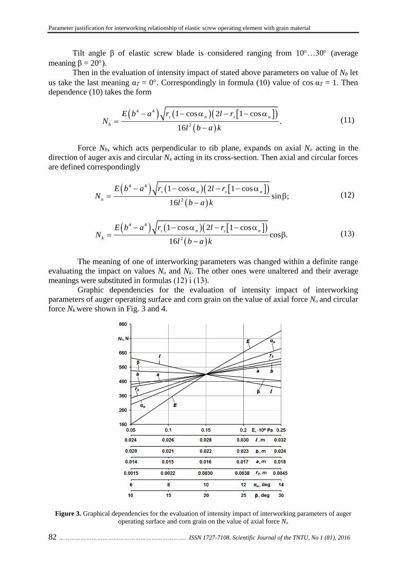
Parameter justification for interworking relationship of elastic screw operating element with grain material
82 ……………………………………………………………. .ISSN 1727-7108. Scientific Journal of the TNTU, No 1 (81), 2016
Tilt angle β of elastic screw blade is considered ranging from 10…30 (average
meaning β = 20).
Then in the evaluation of intensity impact of stated above parameters on value of Nb let
us take the last meaning αТ = 0. Correspondingly in formula (10) value of cos αТ = 1. Then
dependence (10) takes the form
4 4
2
1 cos 2 1 cos.
16
з n з n
b
E b a r l rN
l b a k
(11)
Force Nb, which acts perpendicular to rib plane, expands on axial Nо acting in the
direction of auger axis and circular Nк acting in its cross-section. Then axial and circular forces
are defined correspondingly
4 4
2
1 cos 2 1 cossin ;
16
з n з n
o
E b a r l rN
l b a k
(12)
4 4
2
1 cos 2 1 coscos .
16
з n з n
k
E b a r l rN
l b a k
(13)
The meaning of one of interworking parameters was changed within a definite range
evaluating the impact on values Nо and Nk. The other ones were unaltered and their average
meanings were substituted in formulas (12) і (13).
Graphic dependencies for the evaluation of intensity impact of interworking
parameters of auger operating surface and corn grain on the value of axial force Nо and circular
force Nk were shown in Fig. 3 and 4.
Figure 3. Graphical dependencies for the evaluation of intensity impact of interworking parameters of auger
operating surface and corn grain on the value of axial force Nо
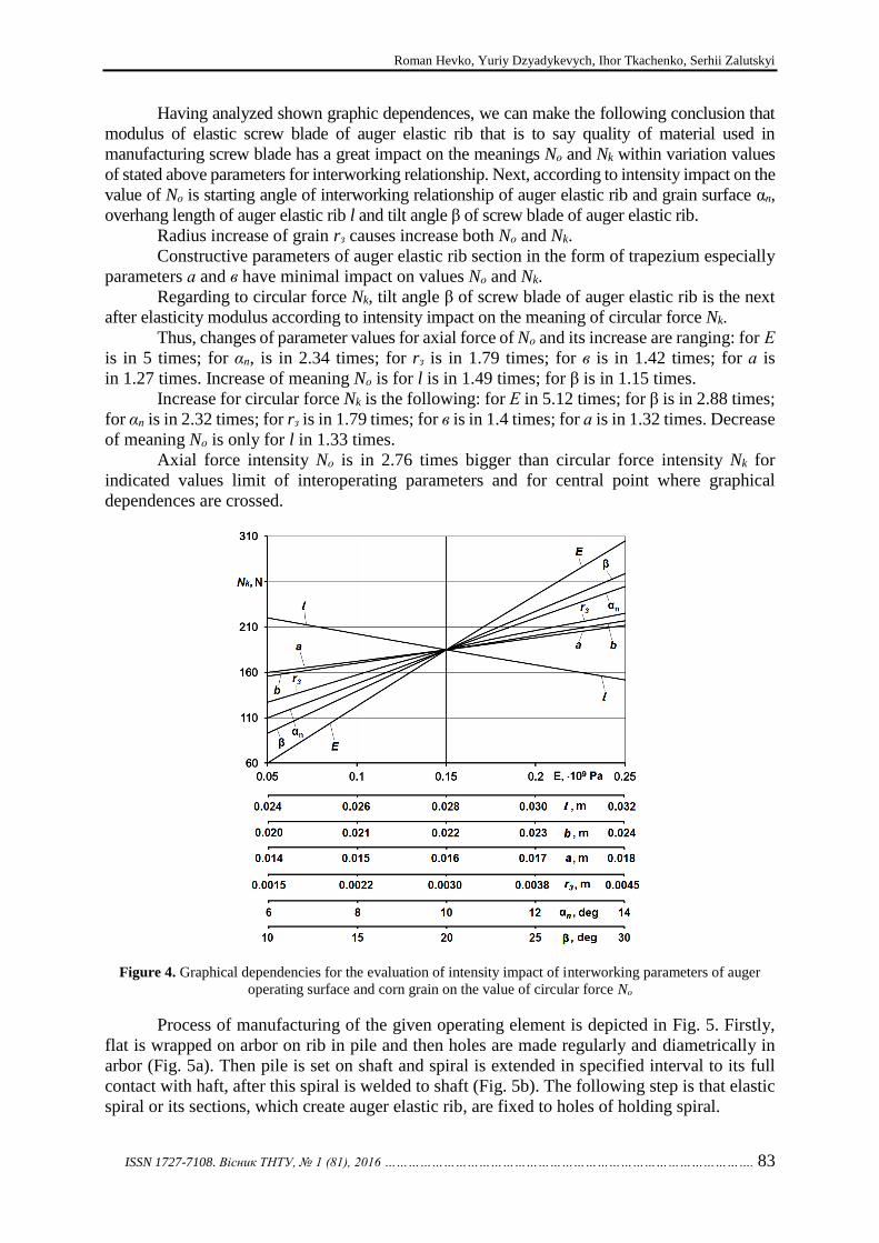
Roman Hevko, Yuriy Dzyadykevych, Ihor Tkachenko, Serhii Zalutskyi
ISSN 1727-7108. Вісник ТНТУ, № 1 (81), 2016 …………………………………………………………………………………. 83
Having analyzed shown graphic dependences, we can make the following conclusion that
modulus of elastic screw blade of auger elastic rib that is to say quality of material used in
manufacturing screw blade has a great impact on the meanings Nо and Nk within variation values
of stated above parameters for interworking relationship. Next, according to intensity impact on the
value of Nо is starting angle of interworking relationship of auger elastic rib and grain surface αп,
overhang length of auger elastic rib l and tilt angle β of screw blade of auger elastic rib.
Radius increase of grain rз causes increase both Nо and Nk.
Constructive parameters of auger elastic rib section in the form of trapezium especially
parameters а and в have minimal impact on values Nо and Nk.
Regarding to circular force Nk, tilt angle β of screw blade of auger elastic rib is the next
after elasticity modulus according to intensity impact on the meaning of circular force Nk.
Thus, changes of parameter values for axial force of Nо and its increase are ranging: for Е
is in 5 times; for αп, is in 2.34 times; for rз is in 1.79 times; for в is in 1.42 times; for а is
in 1.27 times. Increase of meaning Nо is for l is in 1.49 times; for β is in 1.15 times.
Increase for circular force Nk is the following: for Е in 5.12 times; for β is in 2.88 times;
for αп is in 2.32 times; for rз is in 1.79 times; for в is in 1.4 times; for а is in 1.32 times. Decrease
of meaning Nо is only for l in 1.33 times.
Axial force intensity Nо is in 2.76 times bigger than circular force intensity Nk for
indicated values limit of interoperating parameters and for central point where graphical
dependences are crossed.
Figure 4. Graphical dependencies for the evaluation of intensity impact of interworking parameters of auger
operating surface and corn grain on the value of circular force Nо
Process of manufacturing of the given operating element is depicted in Fig. 5. Firstly,
flat is wrapped on arbor on rib in pile and then holes are made regularly and diametrically in
arbor (Fig. 5a). Then pile is set on shaft and spiral is extended in specified interval to its full
contact with haft, after this spiral is welded to shaft (Fig. 5b). The following step is that elastic
spiral or its sections, which create auger elastic rib, are fixed to holes of holding spiral.

Parameter justification for interworking relationship of elastic screw operating element with grain material
84 ……………………………………………………………. .ISSN 1727-7108. Scientific Journal of the TNTU, No 1 (81), 2016
Figure 5. Manufacturing method for auger conveyor with elastic screw blade
Test bench, depicted in Fig. 6 was developed and made for evaluating the impact of
width B and overhang size h of petal (section) of auger elastic rib on its deformation value Δ.
It consists of two hard planks 1, which are compressed together by bolted joints 2. There is
elastic blade 3 between them modeling auger elastic rib section. The bar 4 is fixed to blade
running end on which on the other side is cup for measured weight 6.
Since, load intensity of blade should be insignificant and bar shift should be vertical,
balls of diameter 4.5 mm were used as measured weight to be uniformly distributed on the
bottom of cup.
Because of elastic blade load, its running end bends and deformation value is fixed to
vertical wall 7, where horizontal lines with distance of 1 mm between them are drawn.
Test investigations were done for material of elastic blade «polyurethane PU-60»
2.5 mm thick.
Overhang size and elastic blade width were determined discretely with 5 mm step
ranging: h = 25…10 mm; В = 25…5 mm.
Figure 6. Test bench scheme for evaluation of impact on elastic blade section deformation value Δ of its width B
and overhang size h
Experimental research findings for the dependency of blade running end deformation
value Δ from measured load mass m for different values of В and h were shown in Fig. 7. Having analyzed the given dependencies, we made the following conclusions, that
dependencies are mostly linear, moreover for overhang size of elastic blade h = 25 mm, its
increase in width from 5 to 25 mm causes increase of load intensity for Δ = 2 mm – in 4.9 times;
for Δ = 4 mm – in 5.6 times; for Δ = 6 mm – in 5.8 times; for Δ = 8 mm – in 5.3 times.
For overhang size of elastic blade h = 20 mm, analogical meanings are the following:
for Δ = 2 mm – in 4.8 times; for Δ = 4 mm – in 4.6 times; for Δ = 6 mm – in 4.4 times;
for Δ = 8 mm – in 4.3 times.

Roman Hevko, Yuriy Dzyadykevych, Ihor Tkachenko, Serhii Zalutskyi
ISSN 1727-7108. Вісник ТНТУ, № 1 (81), 2016 …………………………………………………………………………………. 85
For overhang size of elastic blade h = 15 mm, analogical meanings are the following:
for Δ = 2 mm – in 4.8 times; for Δ = 4 mm – in 5.8 times; for Δ = 6 mm – in 5.9 times;
for Δ = 8 mm – in 5.7 times.
For overhang size of elastic blade h = 10 mm, analogical meanings are the following:
for Δ = 2 mm – in 4.8 times; for Δ = 4 mm – in 4.1 times; for Δ = 6 mm – in 4.0 times;
for Δ = 8 mm – in 4.2 times.
Error n between minimal and maximal meanings of increase of load for range
Δ = 2...8 mm and stated above values of elastic blade width is: for h = 25 mm – n = 15.5 %; for
h = 20 mm – n = 10.4 %; for h = 15 mm – n = 18.7 %; for h = 10 mm – n = 16.7 %.
Figure 7. Experimental research findings for the dependency of blade running end deformation value Δ from
measured load mass m for different values of В and h
Experimental research findings for the dependency of impact of overhang size value h
of elastic rib from load mass m in deformation of running rib end Δ = 8 mm were shown
in Fig. 8.
Having analyzed graphical dependencies, depicted in Fig. 8, we can make such
conclusions, that load mass should be increased in 2.8 times, from 180 to 500 gr; for h = 15 mm
in 4.8 times; for h = 20 mm in 4.2 times; for h = 25 mm in 4.3 times for overhang size of elastic
blade h = 10 mm, the increase of its width ranging from В = 5 mm to В = 25 mm for support of
deformation value of running end of elastic blade Δ = 8 mm.
It should be noted that the character of graphical dependences of elastic blade overhang
size h from measured load mass m changes from linear to curvilinear in decreasing of elastic
blade width В.
Conclusions. Based on the patent search analysis of screw operating surfaces and
literary sources concerning the evaluation of their operating modes a new design of auger
conveyor with elastic screw blades and its manufacturing method has been proposed.

Parameter justification for interworking relationship of elastic screw operating element with grain material
86 ……………………………………………………………. .ISSN 1727-7108. Scientific Journal of the TNTU, No 1 (81), 2016
Theoretical predictions have been conducted to evaluate the impact of design
parameters, tilt angles and elasticity coefficient of elastic rib screw as well as its interoperation
specifications with multiple-shaped stuck corn grains on axial and circular force values.
Figure 8. Experimental research findings for the dependency of impact value of elastic blade
overhang size h from measured load mass m at blade running end deformation Δ = 8 mm
Based on theoretical research analysis impact degree of elastic rib screw interoperating
specifications with grain has determined on delimitations that prevent grain bulk damage, and
those specifications have been set, which impose dominant effect on grain decay process.
A test bench for conducting experimental research has been developed and designed.
Experimental research findings have been produced to determine the impact of elastic blade
section, its width, overhang size and measured load mass upon deformation value.
Obtained findings may find practical application in designing different types of auger
operating parts with elastic operating surfaces according to deformation characteristics of
conveying bulk agricultural material and intensity accepted values leading to its decay.
References
1. Herrmann H. Shnekovye mashiny v texnologi. perevod s nem. L. Vedenyapinoj; [pod obshh. red.
M.L. Fridmana], Leningrad, Ximiya, 1975. 232 p. [In Russian]
2. Hevko R.B., Vitrovyi A.O., Pik A.I. Pidvyshchennia tekhnichnoho rivnia hnuchkykh hvyntovykh
konveieriv. monohrafiia, Ternopil, Aston, 2012. 204 p. [In Ukrainian]
3. Hevko R., Klendiy O. Obgruntuvannia parametriv zakhysnykh mekhanizmiv shnekovykh transporteriv.
Visnyk Ternopilskoho natsionalnoho tekhnichnoho universytetu imeni Ivana Puliuia, Naukovyi zhurnal, Ternopil,
Vydavnytstvo TNTU, 2013, no. 2 (70), p.p. 103 – 13. [In Ukrainian]
4. Zenkov R.L., Ivanov N.I., Kolobov L.I. Mashiny nepreryvnogo transporta. Moscow, Mashinostroenie,
1987. 320 p. [In Russian]
5. Hevko R.B. Hlado Y.B., Shynkaryk M.I., Klendiy O.M. Dynamichnyi rozrakhunok zapobizhnoho prystroiu
shnekovoho transportera. Visnyk inzhenernoi akademii Ukrainy, Kyiv, 2014, no 2, p.p. 163 – 168. [In Ukrainian]
6. Hevko R.B., Klendiy O.M. The investigation of the process of a screw conveyer safety device actuation.
INMATEH: Agricultural engineering, Bucharest, 2014, vol. 42, no 1, p.p. 55 – 60.
7. Hevko R.B., Dzyura V.O., Romanovsky R.M. Mathematical model of the pneumatic-screw conveyor screw
mechanism operation. INMATEH: Agricultural engineering, Bucharest, 2014, vol. 44, no 3,
p.p. 103 – 110.
8. Hevko R.B., Zalutskyi S.Z., Tkachenko I.G., Klendiy O.M. Development and investigation of reciprocating
screw with flexible helical surface. INMATEH: Agricultural engineering, Bucharest, 2015, vol. 46, no 2,
p.p. 133 – 138.
9. Hevko R.B., Zalutskyi S.Z. Rozrobka konstruktsii shneka z elastychnoiu hvyntovoiu poverkhneiu ta
rezultaty yii eksperymentalnykh doslidzhen. Visnyk Inzhenernoi akademii Ukrainy, Kyiv, 2015, no. 1,
p.p. 242 – 247. [In Ukrainian]
Roman Hevko, Yuriy Dzyadykevych, Ihor Tkachenko, Serhii Zalutskyi
ISSN 1727-7108. Вісник ТНТУ, № 1 (81), 2016 …………………………………………………………………………………. 87
10. Patent Ukrainy na korysnu model 101095 Ukraine, MPK B65G 33/26. Shnek z elastychnoiu hvyntovoiu
poverkhneiu. Krysovatyi A.I., Hevko R.B., Zalutskyi S.Z., Tkachenko I.G., Hradova M.V. u201502180, zaiavl.
12.03.15 opubl. 25.08.15, Biul. no. 16. [In Ukrainian]
11. Shvabiuk V.I. Opir materialiv: navchalnyi posibnyk. Kyiv, Znannia, 2009. 380 p. [In Ukrainian]
12. Mekhaniko-tekhnolohichni vlastyvosti silskohospodarskykh materialiv: navch. posibnyk. / Tsarenko O.M.,
Voitiuk D.H., Shvaiko V.M. Kyiv, Meta, 2003. 448 p. [In Ukrainian]
Список використаної літератури
1. Геррман, Х. Шнековые машины в технологи [Текст] / Х. Геррман; перевод с нем. Л. Веденяпиной;
под общ. ред. М.Л. Фридмана. – Л.: Химия, 1975. – 232 с.
2. Гевко, Р.Б. Підвищення технічного рівня гнучких гвинтових конвеєрів [Текст]: монографія /
Р.Б. Гевко, А.О. Вітровий, А.І. Пік. – Тернопіль: Астон, 2012. – 204 с.
3. Гевко, Р. Обґрунтування параметрів захисних механізмів шнекових транспортерів [Текст] /
Р. Гевко, О. Клендій // Вісник Тернопільського національного технічного університету імені Івана Пулюя.
Науковий журнал. – 2013. – № 2 (70). – C. 103 – 113.
4. Зенков, Р.Л. Машины непрерывного транспорта [Текст] / Р.Л. Зенков, Н.И. Иванов, Л.И. Колобов. –
М.: Машиностроение, 1987. – 320 с.
5. Гевко, Р.Б. Динамічний розрахунок запобіжного пристрою шнекового транспортера [Текст] /
Р.Б. Гевко, Ю.Б. Гладьо, М.І. Шинкарик, О.М. Клендій // Вісник інженерної академії України. – 2014. –
№ 2. – C. 163 – 168.
6. Hevko, R.B. The investigation of the process of a screw conveyer safety device actuation [Текст] /
R.B. Hevko, O.M. Klendiy // INMATEH: Agricultural engineering. – Bucharest: 2014. Vol. 42, No 1. – P. 55 – 60.
7. Hevko, R.B. Mathematical model of the pneumatic-screw conveyor screw mechanism operation [Текст] /
R.B. Hevko, V.O. Dzyura, R.M. Romanovsky // INMATEH: Agricultural engineering. – Bucharest: 2014. Vol. 44,
№ 3, – P. 103 – 110.
8. Hevko, R.B. Development and investigation of reciprocating screw with flexible helical surface [Текст] /
R.B. Hevko, S.Z. Zalutskyi, I.G. Tkachenko, O.M. Klendiy // INMATEH: Agricultural engineering. – Bucharest:
2015. Vol. 46, № 2. – P. 133 – 138.
9. Гевко, Р.Б. Розробка конструкції шнека з еластичною гвинтовою поверхнею та результати її
експериментальних досліджень [Текст] / Р.Б. Гевко, С.З. Залуцький // Вісник Інженерної академії
України. – 2015. – № 1. – С. 242 – 247.
10. Патент України на корисну модель 101095 Україна, МПК B65G 33/26. Шнек з еластичною
гвинтовою поверхнею [Текст] / Крисоватий А.І., Гевко Р.Б., Залуцький С.З., Ткаченко І.Г., Градова М.В. –
№ u201502180; заявл. 12.03.15 опубл. 25.08.15, Бюл. № 16.
11. Шваб’юк, В.І. Опір матеріалів [Текст]: навчальний посібник / В.І. Шваб’юк. – К.: Знання, 2009. – 380 с.
12. Механіко-технологічні властивості сільськогосподарських матеріалів: навч. посібник [Текст] /
О.М. Царенко, Д.Г. Войтюк, В.М. Швайко та ін. – К.: Мета, 2003. – 448 с.
УДК 631.358.42
ОБГРУНТУВАННЯ ПАРАМЕТРІВ ВЗАЄМОДІЇ ЕЛАСТИЧНОГО
ГВИНТОВОГО РОБОЧОГО ОРГАНУ ІЗ ЗЕРНОВИМ МАТЕРІАЛОМ
Роман Гевко1; Юрій Дзядикевич1; Ігор Ткаченко2; Сергій Залуцький2
1 Тернопільський національний економічний університет, Тернопіль, Україна
2 Тернопільський національний технічний університет імені Івана Пулюя,
Тернопіль, Україна
Резюме. Здійснено аналіз відомих конструкцій робочих органів шнеків з еластичними поверхнями та
процесів роботи гвинтових конвеєрів. Запропоновано нову конструкцію шнека з еластичною гвинтовою
поверхнею та спосіб його виготовлення. Проведено теоретичне обґрунтування щодо визначення впливу
конструктивних і технологічних параметрів еластичної поверхні гвинтового робочого органу на величину
зусиль, що діють на защемлену зернину. Наведено результати експериментальних досліджень щодо
визначення впливу конструктивних параметрів секції еластичної пластини на величину її деформації.
Ключові слова: шнек, еластична гвинтова поверхня, секція еластичної пластини, деформація,
ширина пластини, величина консольного виступу.
Отримано 12.01.2016

Вісник Тернопільського національного технічного університету
Scientific Journal of the Ternopil National Technical University
2016, № 1 (81)
ISSN 1727-7108. Web: visnyk.tntu.edu.ua
88 …………………………………………. Corresponding author: Nemyrovskyy Yakiv; e-mail: [email protected]
UDC 621.735.34.001
ISSUES ABOUT LIMIT PLASTIC DEFORMATIONS OF DEFORMING
BROACHING OF CAST IRON PARTS
Yakiv Nemyrovskyy1; Oleksandr Chernyavskyy1; Pavlo Yeryomin1;
Yuriy Tsekhanov2
1Kirovohrad National Technical University,
Kirovohrad, Ukraine 2Voronezh State University of Architecture and Civil Engineering,
Voronezh, Russia
Summary. Scientific and technical issues about the possibility of deforming broaching of bores in cast
iron parts were investigated in the article. New methods to deform cast iron parts under conditions of all-round
compression were developed. The diagram of plasticity was built according to results of mechanical tests of cast
iron samples. The conditions of plastic deformation of half-brittle cast iron were determined. The dependence of
the resource of cast iron plasticity from structural components and form of graphite inclusions was indicated.
Necessary conditions for effective deforming broaching of bores in cast iron parts were determined. The measure
of plastic deforming broaching of cast iron parts was chosen. The influence of tool geometry, thick walls of a part
and element strain on plasticity during deforming broaching were investigated. The dependence to define limit
deformations during deforming broaching of cast iron parts was suggested.
Key words: deforming broaching, cast iron, plastic deformation.
Received 01.03.16
Problem setting. Graphite cast iron is widely used as a constructive material in modern
mechanical engineering. Traditional methods of deforming broaching of cast iron parts require
considerable time consumption, however more than 80% is for total factory labour hours.
Deforming broaching is a highly productive operation on plastic materials and it is
widely used. The use of this method during deforming broaching of bores in cast iron parts is
restrained by low resource of plasticity of processed material.
The resource of used plasticity is one of important parameter of quality of parts
machined by plastic deforming and characterizes the deficiency of finished surface. In works
[1, 2] it was stated that the plasticity during cold plastic deforming depends on characteristics
of machined material and the history of its deforming.
Consequently, the investigation of this quality parameter during plastic deforming of
cast iron, which is half-brittle and composite material, should be certainly done.
Research objective. To study the possibilities of bores deforming broaching
investigating its resource of plasticity and choice of optimal conditions of deformation.
Review of recent investigations and papers.
The issues of plasticity during deforming broaching were investigated in works
[1, 2, 3], where tense state of machined material on the surface of the contact with the tool
corresponds to volumetric pressure allowing to do considerable plastic deformations. At the
same time, tense state corresponds to double-axis tension. While index of tense state 0
3
(where – hydrostatical pressure, 0 – stress intensity) changes owing to negative meanings
(–7.16) in contact area up to positive meanings (+2) on external surface. It helps to forecast the
beginning of failure during distribution of parts with different thickness of wall near external
surface of a part.

Yakiv Nemyrovskyy, Oleksandr Chernyavskyy, Pavlo Yeryomin, Yuriy Tsekhanov
ISSN 1727-7108. Вісник ТНТУ, № 1 (81), 2016 …………………………………………………………………………………. 89
Therefore, authors [1] suggest to use the directed deformation е' to external surface
depending on relative deformation of tension 0/a d and thick walls of a part 0 0
/t r as
determinative factor according to their investigations. This suggestion is caused by the
following reasons. Conducted investigations regard to deforming broaching of plastic parts
while at their distributions big tensions on considerable total plastic deformations of a bore are
used. Using such big strains, transparent plastic deformation of bore is found that is either
internal or external diameter of a part increases. The degree of used resource of plasticity ,
caused, correspondingly by suggestions [1] made by V. Kolmohorov, is maximum near external
surface where the failure of a part takes place.
Cast iron is known to be half-brittle composite material consisting of ferrite-pearlitic
structure including free graphite of different form presenting brittle component of this
material [4]. Methods and results shown in works [5, 6, 7, 8] are used for investigations of
plastic deforming of cast iron parts.
Research results. Peculiarities of plastic deforming of cast ironware should be
considered. Grey cast iron СЧ20 (hardness HB 1.7 GPa) and high-test cast iron ВЧ50
(HB 2.1 GPa) are widely used in modern mechanical engineering.
Diagram of plasticity (Fig. 1) was constructed to determine possibilities of plastic
deforming of cast ironware that is mechanical characteristic of deformation of cast iron
Figure 1. Diagram of plasticity of grey cast iron СЧ20
According to suggestions [5], to make such diagram, mechanical tests of cast iron under
conditions of simple load and deformation when stresses change proportionally to one
parameter were done. Such tests are of the following types: tension, torsion and compression.
Besides, original methods of testing cast iron under conditions of deformation close to all-round
compression have been developed in the given research.
Tests on tension of cast iron patterns СЧ20 and ВЧ50 were done on special tension
testing machine.
For tests on compression, there were made samples, geometrical sizes of which were
defined according to correlation h/d = 1.5, where h = 15 mm – height of a part; d = 10 – its
diameter. On patterns’ ends, according to suggestions [6], cylindrical grooves about 0.4 mm in
depth and 9.2 mm in diameter were made. Grooves were filled with hard oiling on the base of
varnish Ф-9-К with MoS2 that should support deformations that are more homogeneous. Tests
were made on press ПММ-200 using special instrument providing parallelism of supports.
Compression of samples was made until their failure took place. After failure of samples on
compression and tension, there were made sections on which toughness according to Vickers’
scale was measured at the load Р = 49 N.

Issues about limit plastic deformations of deforming broaching of cast iron parts
90 ……………………………………………………………. .ISSN 1727-7108. Scientific Journal of the TNTU, No 1 (81), 2016
The following methods were used at deformation of cast iron under conditions close to
all-round compression. Research data [7] used at deformation of plastic production were taken
into consideration for the development of the first method. Samples made of investigated
materials of cylindrical form about 35 mm in diameter and h = 15 mm in height were prepared
for using this method. Being previously machined by turning, samples’ ends were polished on
planogrinding machine tool of mod. 3Б71М. Micro-hardness of samples in starting position
and strained state was measured by Vickers’ method using micro-hardness tester «Shimadzu»
(Japan). Load on indenter (diamond pyramid) at measuring micro-hardness of ferrite composite
was 25 gr. and for pearlitic one – 100 gr. Microscope МИМ-7, optical microscope «Altamy»,
raster electronic microscope РЕМ-106И and instrumental microscope БМИ-1 were used to
investigate microstructure of samples and state of machined surface.
Investigations were done according to recommendations [7] in the following way. Hard-
alloyed ball about 10 mm in diameter with effort 30 kN was filled in previously polished
surface. This operation was being processed on hardness tester ТШ-2М during 30 sec. After
removing load, received bore and micro-hardness were measured and external strained area was
observed for magnification. In case of failure on the surface of contact, deforming of sample
was stopped. Surface of samples, where failure was not found out, was polished until initial
diameter of bore was decreased in two times. After this, the sample was put on hardness tester
and repeated cycles of load were done.
After each load, hardness of investigated area of a sample (according to Vickers) in the
range of points situated radially starting from the centre of bore and ending with transition area
was measured. Then, strained samples were cut in the middle of bore in cross-section, filled
with epoxy resin to protect strained area and then they were polished and grinded.
Micro-hardness measuring of strained area was done in three areas (Fig. 2) in the
direction from strained surface to the depth of a sample until hardness of material reached its
initial value.
Figure 2. Dimension scheme of micro-hardness on samples
Dimension step was = 40 mkm. Areas were chosen on these samples, they were
pickled by 5% solution of hydrogen nitrate in ethyl alcohol and then change of areas of ferrite
and pearlite in initial and strained states was investigated.
We have developed one more method of modeling conditions close to all-round
compression reproducing deformation of micro-ends on internal surface of bore deforming
broaching. Model tests were made on samples of conic form made from stated above cast iron
brands with angle 90 according to the scheme (Fig. 3)

Yakiv Nemyrovskyy, Oleksandr Chernyavskyy, Pavlo Yeryomin, Yuriy Tsekhanov
ISSN 1727-7108. Вісник ТНТУ, № 1 (81), 2016 …………………………………………………………………………………. 91
Figure 3. Test materials gain rate device: 1 – conic sample of test material; 2 – high-alloy head;
3 – guide pin bushing
Axial load, which is sufficient for plastic deformation of its top with the next unloading
and measuring of contact area was applied to the top of a sample 1, which was fixed in the iron
band 2, through high-alloy plunger. Besides, axial load was fixed using tensometric
dynamometer of the known design [1].
Sections were made of fractured tested samples. Hardness measurements showed that
in all test points the value of hardness is almost identical and is correspondent to initial hardness
of samples. It shows the absence of strengthening and, thus the absence of plastic deformation
at one-axial tension (that is at =+1).
S. Lopatenko received similar results [8] at defining the limit deformation during
torsion. His experiments showed the absence of visible plastic deformation at torsion
(that is = 0).
The results for deformation of samples of stated above cast iron brands at one-axial
compression should be considered. Experiments, conducted according to method presented
above, supported relatively more homogenous plastic deformations (for high-test cast iron
ВЧ50 up to 50% and for grey cast iron СЧ20 up to 9%). Then sections were made of fractured
samples, which were tested on hardness according to Vickers when load was 49N. Test results
showed that test cast iron samples are essentially strengthened at compression. Thus, hardness
of cast iron ВЧ50 was changed from initial 2 up to 2.95 GPa and cast iron СЧ20 was changed
from 1.7 up to 2.25 GPa, in this case the degree of strengthening was 48 and 30%
correspondingly. Such degree of strengthening shows the availability of considerable plastic
deformations at deforming of cast iron at one-axial compression (that is = –1).
As test results show, the diagram of limit plasticity for cast iron unlike similar diagram
for plastic materials is developed from meanings of deformations which are correspond to
= –1, that is one-axial compression of samples.
The process of deformation of cast iron samples at conditions close to all-round
compression should be considered. The meaning of tense state index is equal to –7 and is
corresponding to this condition.
In Fig. 4 the change of hardness of deformed material on test area after some cycles of
loading is shown, in addition the distance from the centre of bore is put on axis of abscissas and
the hardness according to Vickers is put on axis of ordinates.

Issues about limit plastic deformations of deforming broaching of cast iron parts
92 ……………………………………………………………. .ISSN 1727-7108. Scientific Journal of the TNTU, No 1 (81), 2016
Figure 4. Change of hardness of cast iron СЧ20, НВ1.7 GPa at deformation of a ball in 10 mm at load
Р = 30 kN. Deformation cycles – 1; – 2; – 3; ▼– 4
As it is shown in Fig. 4 at such method of deformation, grey cast iron is under essential
plastic deformations (to 20%), which explains the increase of hardness to HV 2.2 GPa, while
maximum increase of hardness is observed near edge limiting bore. Identical picture is observed
at deformation of high-test cast iron ВЧ50 changing to maximum hardness HV 3.0 GPa.
Tests on modeling conditions close to all-round compression owing to compression of
tops of cast iron cones СЧ20 and high-test cast iron ВЧ50 (Fig. 5) according to stated above
method showed that the dependence of hardness from cycles of additional load is of extreme
nature.
Figure 5. Dependence of hardness of strengthened layer from axial load on the top of cone:
1 – cast iron ВЧ50, 2 – cast iron СЧ20
Initial cone material hardness and hardness after each cycle of deformation were shown
on axis of ordinates. Firstly, at first cycles of deformation, hardness increases and achieves its
maximum while its maximum meaning is correspondent to hardness of identical materials
received at pressing of a ball. Thus, for cast iron СЧ20 maximum meaning of hardness is
HV 2.25 GPa, and for high-test ВЧ50 – HV 3.0 GPa.
Decrease of hardness of cast iron after peak achievement, especially for grey cast iron
СЧ20 was caused by relatively small resource of plasticity of the material leading to micro-
failures on fractured surface of a cone. Limit contraction degree of cones is up to 18% before
failure tracks appear on a fractured surface.
Changes of microstructure of test samples after deformation should be considered.
Microstructure of test samples in initial state is shown in Fig. 6.
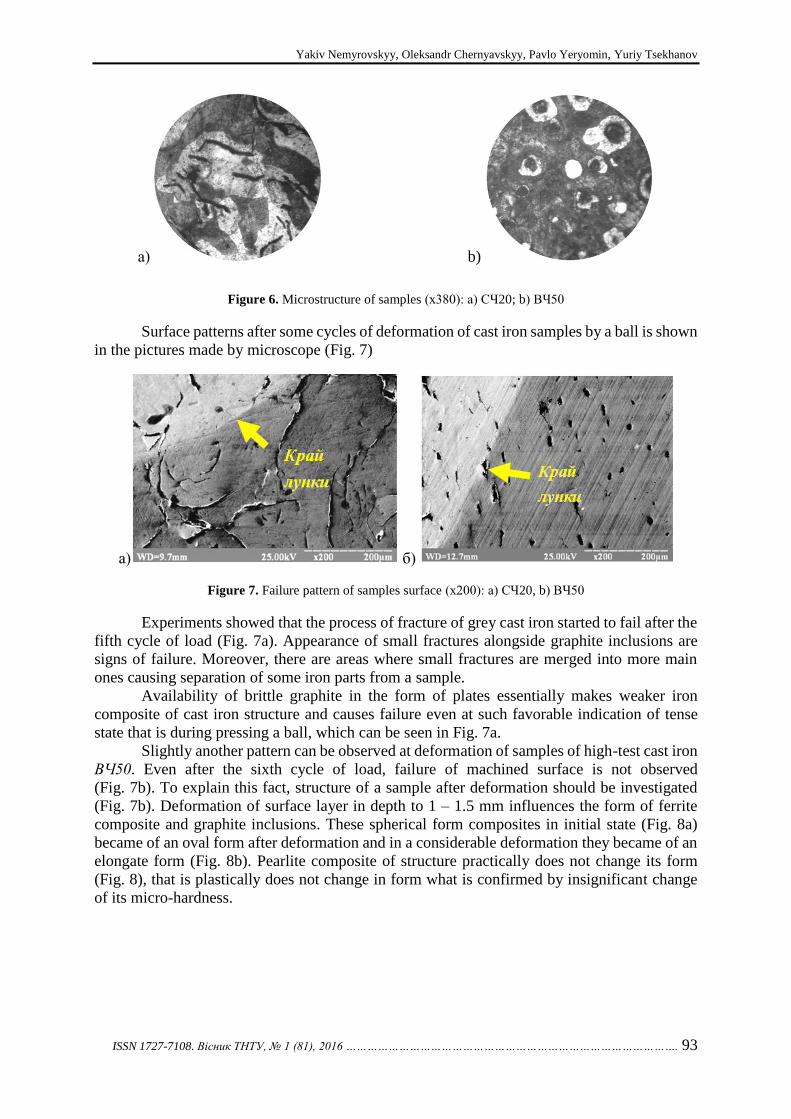
Yakiv Nemyrovskyy, Oleksandr Chernyavskyy, Pavlo Yeryomin, Yuriy Tsekhanov
ISSN 1727-7108. Вісник ТНТУ, № 1 (81), 2016 …………………………………………………………………………………. 93
а) b)
Figure 6. Microstructure of samples (х380): а) СЧ20; b) ВЧ50
Surface patterns after some cycles of deformation of cast iron samples by a ball is shown
in the pictures made by microscope (Fig. 7)
а) б)
Figure 7. Failure pattern of samples surface (х200): а) СЧ20, b) ВЧ50
Experiments showed that the process of fracture of grey cast iron started to fail after the
fifth cycle of load (Fig. 7a). Appearance of small fractures alongside graphite inclusions are
signs of failure. Moreover, there are areas where small fractures are merged into more main
ones causing separation of some iron parts from a sample.
Availability of brittle graphite in the form of plates essentially makes weaker iron
composite of cast iron structure and causes failure even at such favorable indication of tense
state that is during pressing a ball, which can be seen in Fig. 7a.
Slightly another pattern can be observed at deformation of samples of high-test cast iron
ВЧ50. Even after the sixth cycle of load, failure of machined surface is not observed
(Fig. 7b). To explain this fact, structure of a sample after deformation should be investigated
(Fig. 7b). Deformation of surface layer in depth to 1 – 1.5 mm influences the form of ferrite
composite and graphite inclusions. These spherical form composites in initial state (Fig. 8a)
became of an oval form after deformation and in a considerable deformation they became of an
elongate form (Fig. 8b). Pearlite composite of structure practically does not change its form
(Fig. 8), that is plastically does not change in form what is confirmed by insignificant change
of its micro-hardness.

Issues about limit plastic deformations of deforming broaching of cast iron parts
94 ……………………………………………………………. .ISSN 1727-7108. Scientific Journal of the TNTU, No 1 (81), 2016
а) b)
Figure 8. Cast iron structure ВЧ50 (х380): a) in initial state; b) after deformation
If cross-section of bore in area of maximum deformation of material is investigated,
then for cast iron СЧ20, there can be observed areas, where strained grains of graphite forming
micro-fractures are present, which are merged into main fractures (Fig. 9a). Strained graphite
inclusions of spherical and oval form are observed on samples of high-test cast iron (Fig. 9b),
fracture porosity of which is considerably less.
а) б)
Figure 9. Strained area of samples in cross-section of bore (х25), where A – compound (epoxy resin),
Б – body of a sample. а) СЧ20; b) ВЧ50
It explains additionally higher resource of plasticity of high-test cast iron ВЧ50. Consequently, conducted investigations showed that cast iron is deformed plastically
under conditions of deformation close to all-round compression. Resource of plasticity of cast iron depends on its structural composites and form of free graphite.
As it was sated above, limit deformation for plastic materials is considered to be the deformation led to external surface of samples. Investigations conducted at developing a diagram of cast iron plasticity (Fig. 1) showed that its plastic deformation is possible only at negative meanings of index of tense state. Thus, at deforming broaching of cast iron samples it is necessary to avoid cross-section plastic deformation of a sample that is its external surface would not be plastically strained. That is why, plastic area should cover only internal part of a wall of a part. To make theoretical definition of a radius of limit of plastic area is a complex task. So, to determine limit deformation of cast iron samples, experimental methods were used to define limit deformation analyzing experimental results on a phenomenological level.
Total intensity of deformation of a part before failure should be taken into consideration according to suggestions [9] to evaluate quantitatively the meaning of plastic deformation before the failure appears during deforming broaching.
As a result, small plastic deformations appear on cast iron parts and deforming broaching is done by consecutive single deforming elements with identical nominal tensions, it can be suggested that in radial direction on some removing from contact area, deformation is monotonous and close to the scheme of distribution of pipe by internal pressure [1]. In this case, intensity of deformation can be shown in the following form:

Yakiv Nemyrovskyy, Oleksandr Chernyavskyy, Pavlo Yeryomin, Yuriy Tsekhanov
ISSN 1727-7108. Вісник ТНТУ, № 1 (81), 2016 …………………………………………………………………………………. 95
2 2 22
,3
i r z z re e e e e e e (1)
where re , e , z
e – linear deformations in cylindrical coordinates: 0/
r ie t t ;
0/ie r r ;
0/
z ie l l .
Using the condition of incompressibility for ze definition the equation (1) can be shown
in the next form:
2 2
2 2
0 0 0 0
2 2 2 2 i i i ii r r
t t r re e e e e
t t r r
(2)
Dependence (2) was used for definition of limit plastic deformation прe of cast iron
bushes СЧ20 at their machining by deforming elements of different angles . In Fig. 10
dependence 0
i
ae f
d
is shown, from which comes ie , which increases proportionally to
total tension.
Figure 10. Intensiveness dependency of plastic deformations on total tension at deforming broaching of cast iron
parts СЧ20, HCI1.7 GPa with thick wall 0 0/ 0,56t r , tension on element 0/ 0,0028a d , angles of operating
cone: – 2 ; – 4 ; ▼ – 8 ; – 12
In such a case, limit plastic deformation reaches 4%. From Fig. 10 it can be observed that angle of operating cone of deforming element at using small tensions on element practically does not influence the value of limit deformation.
In technological practice, it is convenient to use relative total tension 0
a
d
, as a measure
of deformation of parts. Thickness of wall of a part influences the meaning of limit total tension
0
гр
ae a
d
. The more is thickness of a wall, the higher is the contact pressure as well as
hydrostatic pressure on plastic area, which increases the value of limit deformation a . It is proved by results of experiments (Fig. 11).

Issues about limit plastic deformations of deforming broaching of cast iron parts
96 ……………………………………………………………. .ISSN 1727-7108. Scientific Journal of the TNTU, No 1 (81), 2016
Figure 11. Dependency 0
a
d
on 0 0/t r at deforming broaching of cast iron bushes СЧ20 by deforming elements
with angle 4 and tensions on element 0/a d : 1 – 0.0042; 2 – 0.0028; 3 – 0.0014
As can be seen in Fig. 11, the increase of thickness of a wall of a part causes the increase of limit meaning a . Tension on each deforming element influences the value of limit deformation too. The minimum tension is the most favorable for increase of resource of
plasticity on element ( 0/ 0,0014a d , straight line 1). The value of limit deformation decreases
while relative tension of value of limit deformation increases. Extrapolation of straight
lines 1,2,3 on axis of ordinates, that is 0 0/ 0t r shows the meaning of cast iron deformation at
single-axle tension. For straight line 1 – е=0.7%; for 2 – 0.6%; 3 – 0.5%, which approximately corresponds to limit of elasticity of this material.
Statistical data processing, shown in Fig. 11, allowed receiving the equation:
0
0 0 0
0,008 0,71 0,014 0,71гр
ta ae
d d r
(3)
Conclusions. Having investigated the stated above issues, we can make the following conclusions:
1) Half-brittle cast iron was determined to be plastically strained at negative meanings of tense state index.
2) It was shown that the resource of plasticity depends on structural composites and the form of graphite inclusions at deforming cast iron. However, cast iron has maximum resource of plasticity, where ferrite structure and spherical form of free graphite are prevailing.
3) It was investigated that the main condition for deforming broaching of cast iron parts is the absence of plastic deformation on external surface of a part and plastic deformations should be expand only on internal part of thickness of a wall of a part.
4) It was suggested to evaluate plasticity of cast iron parts at deforming broaching using
the value of total tension 0
a
d
before the failure, which does not depend on angle of operating
cone of deforming element and increases while thickness of a wall of a part increases and tension on each deforming element decreases.
5) The dependence to define limit deformations at distribution of cast iron parts determining necessary quantity of deforming elements and distribution of tensions has been suggested. References
1. Tsehanov Yu. A. Mehanika formoobrazovaniya zagotovok pri deformiruyuschem protyagivanii, Yu. A. Tsehanov, S. E. Sheykin, Voronezh, VGTA, 2001. – 203 p. [in Russian]
2. Smelyanskiy V.M. Mehanika uprochneniya detaley poverhnostnyim plasticheskim deformirovaniem. – M. Mashinostroenie. – 300 p. [in Russian]
3. Tsehanov Yu. A. Mehanika deformiruyuschego protyagivaniya, kak nauchnaya osnova otsenki kachestva detaley i rabotosposobnosti instrumenta s iznosostoykimi pokryitiyami. Avtoreferat diss. dokt. tek. nauk, 05.02.08, KPI. – Kiev, 1993. – 43 p. [in Russian]

Yakiv Nemyrovskyy, Oleksandr Chernyavskyy, Pavlo Yeryomin, Yuriy Tsekhanov
ISSN 1727-7108. Вісник ТНТУ, № 1 (81), 2016 …………………………………………………………………………………. 97
4. Gulyaev A.P. Metallovedenie. – M.: Metallurgiya, 1978. – 646 p. [in Russian] 5. Ogorodnikov V.A. Otsenka deformiruemosti metalla pri obrabotke davleniem. – Kiev: Vischa shkola,
1983. – 175 p. [in Russian] 6. Metodika ispyitaniy pri bolshih odnorodnyih plasticheskih deformatsiyah, V.I. Levitas, A.B. Nemirovskiy,
I.E. Stashkevich, A.V. Chernyavskiy, Prochnost, plastichnost i novyie protsessyi polucheniya i obrabotki materialov. – Minsk: Nauka i tehnika, 1985. – pp. 14 – 15. [in Russian]
7. Rozenberg A.M., Rozenberg O.A., Krivosheya V.V. Uprochnenie poverhnosti pri deformiruyuschem protyagivanii vtulok s beskonechnoy tolschinoy stenki i sposob opredeleniya predelnogo uprochneniya, Rezanie i instrument: Resp. mezhved. nauchn-tehn. sb. – no. 33. – Harkov: Vischa shkola, 1985. – pp. 103 – 107. [in Russian]
8. Lopatenko S.G. Osobennosti deformiruyuschego protyagivaniya neravnozhestkih detaley iz chuguna: Avtoreferat. diss. kand. tek. nauk. spets. 05.03.01 «Protsessyi mehanicheskoy obrabotki, stanki i instrument», S.G. Lopatenko – Kiev, 1998. – 16 p. [in Russian]
9. Smirnov-Alyaev G.A. Soprotivlenie materialov plasticheskomu deformirovaniyu – Moskva – Leningrad: Mashgiz, 1961. – 464 p. [in Russian] Список використаної літератури
1. Цеханов, Ю.А. Механика формообразования заготовок при деформирующем протягивании [Текст] / Ю.А. Цеханов, С.Е. Шейкин // Воронеж, ВГТА, 2001. – 203 с.
2. Смелянский, В.М. Механика упрочнения деталей поверхностным пластическим деформированием [Текст] / В.М. Смелянский. – М. Машиностроение. – 300 с.
3. Цеханов, Ю.А. Механика деформирующего протягивания, как научная основа оценки качества деталей и работоспособности инструмента с износостойкими покрытиями [Текст] / Ю.А. Цеханов //Автореферат дис. … докт. техн. наук /05.02.08/КПИ. – Киев, 1993. – 43 с.
4. Гуляев, А.П. Металловедение [Текст] / А.П. Гуляев. – М.: Металлургия, 1978. – 646 с. 5. Огородников, В.А. Оценка деформируемости металла при обработке давлением [Текст] /
В.А. Огородников. – Киев: Вища школа, 1983. – 175 с. 6. Методика испытаний при больших однородных пластических деформациях [Текст] / В.И. Левитас,
А.Б. Немировский, И.Е. Сташкевич, А.В. Чернявский // Прочность, пластичность и новые процессы получения и обработки материалов. – Минск: Наука и техника, 1985. – С. 14 – 15.
7. Розенберг, А.М. Упрочнение поверхности при деформирующем протягивании втулок с бесконечной толщиной стенки и способ определения предельного упрочнения [Текст] / А.М. Розенберг, О.А. Розенберг, В.В. Кривошея // Резание и инструмент: Респ. межвед. научн-техн. сб. – Вып. 33. – Харьков: Вища школа, 1985. – С. 103 – 107.
8. Лопатенко, С.Г. Особенности деформирующего протягивания неравножестких деталей из чугуна: автореф. дис. … канд. техн. наук спец. 05.03.01 «Процессы механической обработки, станки и инструмент» [Текст] / С.Г. Лопатенко. – Киев, 1998. – 16 с.
9. Смирнов-Аляев, Г.А. Сопротивление материалов пластическому деформированию [Текст] / Г.А. Смирнов-Аляев. – Москва – Ленинград: Машгиз, 1961. – 464 с.
УДК 621.735.34.001
ДО ПИТАННЯ ПРО ГРАНИЧНІ ПЛАСТИЧНІ ДЕФОРМАЦІЇ ЗАГОТОВОК ІЗ ЧАВУНУ, ОБРОБЛЕНИХ ДЕФОРМУВАЛЬНИМ
ПРОТЯГУВАННЯМ
Яків Немировський1; Олександр Чернявський1; Павло Єрьомін1; Юрій Цеханов2
1Кіровоградський національний технічний університет, Кіровоград, Україна
2Воронезький державний архітектурно-будівельний університет, Воронеж, Росія
Резюме. Розглянуто науково-технічні питання можливості обробки отворів у деталях із чавуну деформувальним протягуванням. Розроблено нові методики деформування зразків з чавуну в умовах всебічного стиску. За результатами механічних випробувань зразків із чавуну побудовано діаграму пластичності. Установлено умови пластичного деформування напівкрихкого чавуну. Показано залежність ресурсу пластичності чавуну від структурних складових та форми графітових включень. Установлено необхідні умови для ефективної обробки отворів у заготовках із чавуну деформувальним протягуванням. Вибрано міру пластичності при деформувальному протягуванні чавунних заготовок. Вивчено вплив геометрії інструмента, товстостінності заготовки та натягу на елемент на пластичність при деформувальному протягуванні. Запропоновано залежність для визначення граничних деформацій при деформуванні заготовок із чавуну.
Ключові слова: деформувальне протягування, чавун, пластична деформація.
Отримано 01.03.16

Вісник Тернопільського національного технічного університету
Scientific Journal of the Ternopil National Technical University
2016, № 1 (81)
ISSN 1727-7108. Web: visnyk.tntu.edu.ua
98 ……………………………………………….. Corresponding author: Vakulenko Oleksandr; e-mail: [email protected]
INSTRUMENT-MAKING
AND INFORMATION-MEASURING SYSTEMS
ПРИЛАДОБУДУВАННЯ
ТА ІНФОРМАЦІЙНО-ВИМІРЮВАЛЬНІ СИСТЕМИ
UDC 519.241.2; 621.317.333.6
FEATURES OF STATISTICAL DATA PROCESSING AT INSULATION
TESTING OF ENAMELED ELECTRIC WIRES
Petro Yevtukh; Oleksandr Vakulenko
Ivan Puliui National Technical University of Ternopil, Ternopil, Ukraine
Abstract. The necessity of checking of variation series of voltage by insulation breakdown of enameled
wire for the sharply differing values from statistical laws is substantiated. The need for additional research of
causes of abnormal values of voltage breakdown of enameled wires insulation within standard testing methods is
established. The methodology of enameled wire insulation testing by high voltage to evaluate the degree of their
defectiveness using methods of statistical analysis is developed. The advantage of statistical modeling in the study
of enameled coating directly in the locations of indulgence and insulation defects is proved.
Key words: enameled wire, high voltage tests, insulation defects, statistical methods. Received 02.12.15
Problem setting. Requirements for enameled wires used to manufacture winding
elements of electrical devices, envisage (2 ... 3) – time breakdown voltage exceeding of lacquer
layer of wire insulation, measured using a standard method of double wire «twist» samples
according to IEC 60317-0-1 (GOST 14340.7-74), above standard value, which is considered a
reasonable level of quality assurance of the winding technological process [1].
However, conducted control tests on winding elements after their winding process prove
that the given excess does not always guarantee their quality. Moreover, testing has also
revealed that the above stock voltage breakdown mostly does not exist due to peculiarities of
the breakdown in the discharge gap of the standard sample.
This disadvantage of standard methodology is due to the fact that the breakdown of
insulation is conducted under the scheme «dielectric – air – dielectric». The same occurs to the
dielectric where there is insulation derogation and some defects.
The presence of the air layer in the discharge gap significantly alters the largest voltage
breakdown of lacquer layer of enameled wire and causes it considerable variation, «masking»
thus the real state of insulation, especially in its minimum voltage breakdown in the controlled
samples [2].
Therefore, the standard method of determining the breakdown voltage insulation of
enameled wire can be considered only as determining one with low information content of its
defectiveness.
However, extreme values of the insulation voltage breakdown variations series from
enameled wire sample the statistical test results in the recommended literature are often
contradictory. Thus, the standard method of testing insulation using samples such as double

Petro Yevtukh, Oleksandr Vakulenko
ISSN 1727-7108. Вісник ТНТУ, № 1 (81), 2016 …………………………………………………………………………………. 99
wire «twist» allows rejection lowest from the five values of breakdown voltage insulation
without appropriate regulation. The majority of special regulations (e.g. ISO GOST
5725-2:2005), including developed standards instead of outdated ones, recommend the
researcher to reject and do not take into account the «problem» results of measurements that
disturb statistical regularity of variation members.
The basis of the recommendations constitutes the techniques of the well-known
researcher of statistical series Grubbs, in which a number of variations can be used to detect the
minimum (maximum) anomalous values or both [3]. B. Lemeshko’s recommendations are a
further development of Grubbs’ methods on the allocation of the normal number of variations
of several anomalous minimum or maximum values in their various combinations [4]. Thus the
presence of such values inevitably affects the measurement of dispersion and other studied
characteristics of scattering value. Therefore, using Grubbs’ criteria it is necessary to test
statistical sample, consistently increasing the amount of the potential anomalous values.
More closer to reality are such researchers as M. Shcherbakov, A. Orlov, who cast doubt
on the allegations of a comprehensive broad applicability of normal distribution and
recommend a cautious attitude as to remove measurements that sharply differ, for safety reasons
underlying statistical analysis and so as to the allocation of the special values in the statistics
that may indicate the presence of new physical effect [5].
The purpose of the work is to suggest, using metrological analysis, new approaches to
consideration of abnormal values in statistical research samples of electric strength of enameled
wires insulation for a more adequate assessment and mathematical description of its
defectiveness.
Material and methodology of the research. The study involved the most common for
the winding elements of electrical machines and apparatus enameled wires of the following
makrs PET – 155 TU U 31.3-20006134-015:2004, PET–155 GOST 21428-75, PETD – 200 TU
U 31.3-20006134-014:2004, PETD2 – 200 TU U 13970259.001-97 and PEEIDKH2 – 200 TU
U 31.3-0021534.035:2005 of nominal diameters from 0.18 to 1.50 mm.
The program includes the following studies of enameled wires insulation:
- establishing of normality of dispersion values of voltage breakdown of air gaps
between weakened spots or defective insulation ones;
- metrological research of the breakdown voltage abnormal values;
- definition and mathematical description of the spread of values of real electric strength
of weakened spot of insulation defect locations during testing its electric strength.
To implement the program the following research methods are used:
- breakdown voltage insulation of the investigated enameled wire is determined using
standard double wire «twists» according to the methods IEC 60317-0-1 (GOST 14340.7-74).
Processing of the received measurements for determining the metrological characteristics of the
distributions of voltage breakdown is done with GOST ISO 5725-2:2005 method;
- dielectric strength of the lacquer insulation layer in defects spots is determined by
«continuous contact» according to [6].
Research results. For research the impact of technological and structural factors during
manufacture of winding elements of various structural dimensions on the lacquer layer of
enameled wire insulation, they are unwind without insulation damage and the electric strength
along the element is determined.
Sample of the groups controlled by electric vehicles (semi-finished) are tested. Their
winding elements are made, for example, from enameled wire mark PET–155-0.56 TU U 31.3-
20006134-015:2004 as rectangular products with combined folding frame and aspect ratio
(2.0 ... 2.5): 1 with 900 convolutions and their winding speed is about 1600 turns / min.-1 on
one and the same winding machine.
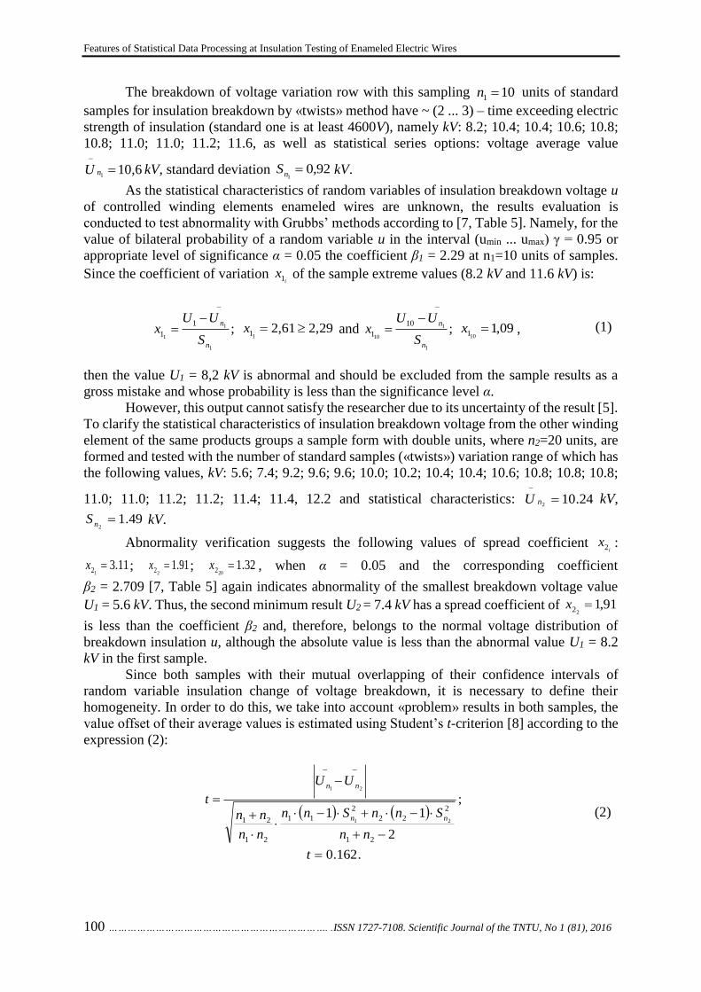
Features of Statistical Data Processing at Insulation Testing of Enameled Electric Wires
100 ……………………………………………………………. .ISSN 1727-7108. Scientific Journal of the TNTU, No 1 (81), 2016
The breakdown of voltage variation row with this sampling units of standard
samples for insulation breakdown by «twists» method have ~ (2 ... 3) – time exceeding electric
strength of insulation (standard one is at least 4600V), namely kV: 8.2; 10.4; 10.4; 10.6; 10.8;
10.8; 11.0; 11.0; 11.2; 11.6, as well as statistical series options: voltage average value
kV, standard deviation kV.
As the statistical characteristics of random variables of insulation breakdown voltage u
of controlled winding elements enameled wires are unknown, the results evaluation is
conducted to test abnormality with Grubbs’ methods according to [7, Table 5]. Namely, for the
value of bilateral probability of a random variable u in the interval (umin ... umax) γ = 0.95 or
appropriate level of significance α = 0.05 the coefficient β1 = 2.29 at n1=10 units of samples.
Since the coefficient of variation of the sample extreme values (8.2 kV and 11.6 kV) is:
and , (1)
then the value U1 = 8,2 kV is abnormal and should be excluded from the sample results as a
gross mistake and whose probability is less than the significance level α.
However, this output cannot satisfy the researcher due to its uncertainty of the result [5].
To clarify the statistical characteristics of insulation breakdown voltage from the other winding
element of the same products groups a sample form with double units, where n2=20 units, are
formed and tested with the number of standard samples («twists») variation range of which has
the following values, kV: 5.6; 7.4; 9.2; 9.6; 9.6; 10.0; 10.2; 10.4; 10.4; 10.6; 10.8; 10.8; 10.8;
11.0; 11.0; 11.2; 11.2; 11.4; 11.4, 12.2 and statistical characteristics: kV,
kV.
Abnormality verification suggests the following values of spread coefficient :
; ; , when α = 0.05 and the corresponding coefficient
β2 = 2.709 [7, Table 5] again indicates abnormality of the smallest breakdown voltage value
U1 = 5.6 kV. Thus, the second minimum result U2 = 7.4 kV has a spread coefficient of
is less than the coefficient β2 and, therefore, belongs to the normal voltage distribution of
breakdown insulation u, although the absolute value is less than the abnormal value U1 = 8.2
kV in the first sample.
Since both samples with their mutual overlapping of their confidence intervals of
random variable insulation change of voltage breakdown, it is necessary to define their
homogeneity. In order to do this, we take into account «problem» results in both samples, the
value offset of their average values is estimated using Student’s t-criterion [8] according to the
expression (2):
(2)
101 n
6,101
nU 92,01nS
ix1
;
1
1
1
1
1
n
n
S
UUx
29,261,2
11 x ;
1
1
10
10
1
n
n
S
UUx
09,1
101 x
24.102
nU
49.12nS
ix2
11.312 x 91.1
22 x 32.1202 x
91,122 x
;
2
11
21
2
22
2
11
21
21 21
21
nn
SnnSnn
nn
nn
UU
t
nn
nn
.162.0t

Petro Yevtukh, Oleksandr Vakulenko
ISSN 1727-7108. Вісник ТНТУ, № 1 (81), 2016 …………………………………………………………………………………. 101
With the value of bilateral probability of a random variable u in the interval (umin ... umax)
γ = 0.95 and the number of degrees of freedom ; k = 28, according to [8]
confidence factor is . Thus, according to this criterion of compatibility
sample medium and are differ insignificantly and samples can be considered as being
derived from a general summation of the random variable u.
The results of some research [9] may question the latter conclusion, arguing that the
t-criterion only allows to test the hypothesis of equality of mathematical expectations
considering the limited volume samples (at least two orders of magnitude). Instead of Students’
criteria to test homogeneity Cramer – Welch’s T-criterion is proposed to use being based on
such statistics (3) which adapted for these studies:
. (3)
There follows a decision based on asymptotic normality of T-statistics: if ,
where , – quantile of normal distribution with probability p (in this case – the critical
value for significance level α), then the hypothesis of homogeneity (equality) mathematical
expectations is taken at significance level α. This means that investigating the statistical
characteristics of both samples (including their anomalous values) with probability γ = 0.95
from equation (3) a disparity is received which confirms this hypothesis:
.
Admissibility of average-deviation spread is checked using Fisher’s F-criterion [10]
according to (4) with regard to anomalous values of breakdown voltage and inequality :
, (4)
where for value γ = 0.95 with the numbers of freedom degrees ; and ;
formed by the expression (4) inequality [7] indicates equal
accuracy of the conducted measurements of enameled wire insulation voltage breakdown of
both samples according to standard «twists» method. The measurements themselves are devoid
of systematic error.
Finally, as both samples contain some anomalous values and are homogeneous, it can
be suggested that understated abnormal voltages have some information about technological
and constructive factors. These ones act on the enameled wire insulation in the process of
winding elements formation whose essence is not disclosed by this standard method of testing.
Their movement beyond confidence intervals of values of the random variable indicates a slight
deviation from the normal distribution of the insulation breakdown voltage.
Rank nonparametric Wilcoxon’s T-criterion is applied to prove deviation from the
normal law of insulation voltage breakdown values in both samples and homogeneity of the
results. According to this criterion [9] two samples of experimental data: and
are considered as relatively homogeneous comparing to their average
221 nnk
ttt 048,295,0
1nU
2nU
2
1
2
2
21
21
21
nn
nn
SnSn
UUnn
T
21
uT
puu
21
96,1814,0 975,0 uT
12 nn SS
122
2
211
;;
1
1
2 ffFS
SF
ffF n
n
111 nf 91 f 122 nf
192 f 908,2623,2396,0
1...,, 21 nxxx
2...,, 21 nyyy 512 nn

Features of Statistical Data Processing at Insulation Testing of Enameled Electric Wires
102 ……………………………………………………………. .ISSN 1727-7108. Scientific Journal of the TNTU, No 1 (81), 2016
arithmetic, if the calculated value of the sum satisfies the condition:
(5)
where Ri – elements ranks xi-yi in both samples, equal to their numbers (1, 2, ... 30) in the ranking
table according to the variational series of insulation voltage breakdown [8];
– mathematical expectation of the rank sum W;
– variance of the rank sum W;
– quantile of normal distribution (see (3)).
The following components of Wilcoxon’s T-criterion are received as a result of
compiling rank table and the corresponding calculations: W = 168.5 ≈ 169; M(W) = 155;
D(W) ≈ 517.
Since in the process of ranking revealed some spots of interconnectedness of both
variational series, variance D (W) is adjusted by the factor kW according to the expression (6):
;
,
(6)
where ti – size l connection, which includes ranks in both samples. According to the ranking
table one can received: t1 = 4; t2 = 2; t3 = 5; t4 = 4; t5 = 3.
Thus, according to (5) and (6) obtained inequality indicates the validity
of the null hypothesis about homogeneity of the two sample distributions of enameled wire
insulation breakdown voltage which differs from the normal law.
To eliminate uncertainty about abnormal voltage values by insulation breakdown there
has been developed a special technique to diagnose enameled wires. Given method allows
increasing accuracy and informative contents of test results compared to the standard ones. In
addition, it provides opportunity to bind defects to the technological level during manufacturing
winding items of electrical equipment, and the homogeneity of lacquer layer of enameled wire
in the initial state. The methodology has been verified by numerous tests and based on the patent
use [6]. As a result of the experiment a statistical number of discrete values of minimum
quantities of insulation voltage breakdown in its most heterogeneous, clearly weakened or
defected locations, normalized to a unit of length of enameled wire is obtained.
The most effective mathematical laws for modeling distributions of breakdown voltage
insulation of enameled wire, taking into account their existing asymmetry and kurtosis are
derived from normal distribution convergent Gram-Charlier’s statistical series, which is
described using the density distribution function by equation [10]:
, (7)
1
1
n
i
iRW
21
uWD
WMWT
2
1211
nnnWM
12
12121
nnnnWD
96,1975,0
21
uu
11
1
1212121
1
2
nnnnnn
tt
k
l
i
ii
W
99.001,01 Wk
96,162,0 T
xfS
xxS
xxfIVIIIk
S
246

Petro Yevtukh, Oleksandr Vakulenko
ISSN 1727-7108. Вісник ТНТУ, № 1 (81), 2016 …………………………………………………………………………………. 103
where – density of the standard normal distribution; , – 3rd and 4th
derivatives order of the function ; , – asymmetry and kurtosis of investigational
distribution.
The method of «continuous contact» according to [6] is used to test given above
enameled wires in course of the research program. Synthesized result is shown below in the
following example of the same make of enameled wire mark PET–155–0.56 TU
U 31.3-20006134-015: 2004 mounted from winding element of the investigated group using
the methodology in [11].
The distribution of voltage by insulation breakdown N1 = 34 units of samples along
array of winding element and N2 = 16 units at the beginning of winding in their intervals ΔU
are given in Table 1, where the number of intervals in accordance with Sturges’ rules r = 7;
nU – interval number of samples; h – value of interval voltage change, kV.
Table № 1.
The distributions of enameled wire insulation breakdown voltage PET – 155 – 0.56
ΔU1, кV [1.54 ...
2.24)
[2.24 …
2.94)
[2.94 …
3.64)
[3.64 …
4.34)
[4.34 …
5.04)
[5.04 …
5.74
[5.74 …
6.40)
nU1 1 3 10 8 7 3 2
ΔU2, кV [0.46 ...
0.60)
[0.60 …
0.74)
[0.74 …
0.88)
[0.88 …
1.02)
[1.02 …
1.16)
[1.16 …
1.30
[1.30 …
1.44)
nU2 2 4 4 2 2 1 1
As a result of these calculations the following statistical characteristics of insulation
breakdown voltage are obtained:
- mathematical expectation М1(U) = 3.99 кV; М2(U) = 0.86 кV;
- mode ℳ1 ≈ 3.29 кВ < M1(U); ℳ2 ≈ 0.76 кВ < M2(U);
- standard deviation 1(U) = 1.01 кV; 2(U) = 0.24 кV;
- asymmetry Sk1 = +0.24 ≥ 0; Sk2 = +0.60 ≥ 0;
- kurtosis ε1 = – 0.60 ≤ 0; ε2 = – 0.50 ≤ 0.
Given the existing asymmetry, it is assumed that the distribution of insulation
breakdown voltage is mathematically described by Gram-Charlier’s statistics (7) with the
computed coefficients Sk , and ε and relative frequency ws (8):
. (8)
Then the relative frequencies distributions of insulation breakdown voltage of enameled
wire along winding element and at the beginning winding according to the simulation results
can be presented by the following expressions, respectively:
; ;
; .
Fig. 1 shows graph distribution functions of given voltage U by insulation breakdown
of enameled wire mark PET-155-0.56, winded off from the winding element.
x xIII x
IV
x kS
3624
36
12
1 2222
2
yyyyS
eU
hw k
y
S
36025.03039.012
1
01.1
70.0 2
1
2
1
2
112
21
1
yyyyew
y
S 01.1
99.31
Uy
36021.031.012
1
24.0
14.0 2
2
2
2
2
222
22
2
yyyyew
y
S 24.0
86.02
Uy

Features of Statistical Data Processing at Insulation Testing of Enameled Electric Wires
104 ……………………………………………………………. .ISSN 1727-7108. Scientific Journal of the TNTU, No 1 (81), 2016
Figure 1. Graphs of distribution functions of insulation breakdown voltage:
F1* – along winding element without beginning of the coiling; Fs1 – is the same, according to the simulation
results; F2* – beginning of the coiling; Fs2 – is the same, according to the simulation results.
To confirm the hypothesis of test precision modeling, namely Kolmogorov’s parametric
test (D – criterion), [10] is used. Having calculated the corresponding statistical distribution
function F*(x) and theoretical (integral) distribution function F(x) parameter λ in this criterion
is defined:
; , (9)
where D = 0.040; λ1 = 0,23; λ2 = 0.27.
Then [10], the numerical value of probability : P1(0.23) ≈ 1.0
and P2(0.27) ≈ 1.0 indicates the validity of the accepted hypotheses.
Since the threshold and nominal dielectric strength of insulation enameled wire mark
PET-155-0.56 with diametrical insulation thickness of (0.052 ... 0.060) mm is respectively:
kV∙mm-1 ≥ 20 kV∙mm-1
and
kV∙mm-1 ≥ 150 kV∙mm-1,
then according to [6] investigated enameled wire along winding element should be attributed
to the classification group: insulation with an average degree of defectiveness.
The same characteristics apply to coiling at the beginning, respectively:
kV mm-1 ≤ 20 kV∙mm-1
and
kV∙mm-1 ≤ 100 kV∙mm-1,
and therefore, according to [6] the researched enameled wire at the early stage of coiling of the
winding element should be attributed to the classification group: insulation with a high degree
of defectiveness. The most probable electrical insulation strength of this segment is:
ND UFUFD *
max
j
jjeP
222
11
96...82060.0...052.0
52.2...46.221.01
threshE
170...146060.0...052.0
42.4...38.4275.01
nomE
20...16060.0...052.0
52.0...46.021.02
threshE
36...30060.0...052.0
92.0...88.0275.02
nomE
0
0,2
0,4
0,6
0,8
1
0 0,5 1 1,5 2 2,5 3 3,5 4 4,5 5 5,5 6 U, кВ
F1*
Fs1
F2*
Fs2

Petro Yevtukh, Oleksandr Vakulenko
ISSN 1727-7108. Вісник ТНТУ, № 1 (81), 2016 …………………………………………………………………………………. 105
kV∙mm-1,
which is (5 ... 7) times less than electric insulation strength values of enameled wire along
winding element.
Therefore, researches using methodologies [6] is found that at manufacturing of the
winding elements party of electrical apparatus from the enameled wire mark PET-155-0.56
TU U 31.3-20006134-015:2004 its insulation at the beginning of winding as a result of
intensive technological factors gets significant damage. However, these damages visualize in
the tests using standard methodology only as implied «emission» of distribution statistical law.
It should be noted that a significant variation of enameled wire insulation breakdown
voltage along the array of coiling element with obvious asymmetry towards small values
indicates its heterogeneity, and increased breakdown probability due to the relative position of
defective insulation spots at critically short distances within its thickness. During its
exploitation the longitudinal defectiveness of insulation only increases, negatively acting on the
operating time of winding element in electrical devices.
Conclusions. Insufficient informative contents of the widely used metrological
procedures of objects research such as insulation electric strength of enameled wires using
standard methods of their testing is detected.
The necessity of taking into account and additional research of abnormal test results
without systematic errors, to improve the diagnosing efficiency of objects research is
substantiated.
The proposed methodology is more accurate instrument for insulation research of the
enameled wire. It enables improvement of information content of the existing standard
methodologies, especially at presence in statistical samples minimal values of insulation
breakdown voltage, which are substantiated by metrological procedures as abnormal.
The developed methodology enables to mathematically describe the breakdown voltage
random variables distributions in weakened locations and insulation defects of enameled wires
by using the derived from normal law Gram-Charlier’s statistical series. The method makes it
possible to create mathematical models that take into account the real insulation defectiveness
both in the initial state of enameled wire and as a result traumatic actions of technological
factors during manufacturing of electrical products with winding elements.
References
1. Delivery Instructions for Round Enamelled Winding Wires. LS–QW–03. Vossloh Schwabe Urbach,
1993, 6 p.
2. Yevtukh P.S., Vakulenko O.O. Doslidzhennia informatyvnosti metodiv vyprobovuvan napruhoiu
emalovanykh provodiv. Enerhetyka i avtomatyka – Energy and Automation, 2013, Vol. 2, pp. 20 – 31
[in Ukrainian].
3. Grubbs F., Beck G. Extension of sample sizes and percentage points for significance tests of outlying
observations, Technometrics, 1972, Vol. 14, no. 4, pp. 847 – 854.
4. Lemeshko B.Yu. Rasshyreniie oblasti primienieniia kritieriiev tipa Grabbsa, ispolzuiemykh pri otbrakovkie
anomalnykh izmierienii. Izmieritielnaia tiekhnika – Measuring technology, 2005, Vol. 6, pp.13 – 19 [in Russian].
5. Orlov A.I. O sovriemennykh probliemakh vniedrieniia prikladnoi statistiki i druhikh statistichieskikh
mietodov. Zavodskaia laboratoriia – Factory Laboratory, 1992, Vol. 1, pp. 67 – 74 [in Russian].
6. Patent Ukrainy 54560 UA, IPC 7 G01R31/12 Sposib otsinky stupenia defektnosti izoliatsii emalprovodiv.
Vakulenko O.O.; zaiavnyk VAT «Vatra», № 2000042307; zaiavlenyi 24.04.2000; opublikovanyi 17.03.2003,
Biuleten № 3/2003 [in Ukrainian].
7. Tochnost (pravilnost i prietsizionnost) mietodov i riezultatov izmierienii. Chast 2 Osnovnoi mietod
opriedielieniia povtoriaiemosti i vosproizvodimosti standartnoho mietoda izmierienii. GOST R ISO 5725–2–
2002. Moskva, Izdatielstvo standartov, 2002, 43 p. [in Russian].
8. Danilchienko V.P., Yehoshyn R.A. Mietrolohichieskoie obiespiechieniie promyshliennoho proizvodstva:
Spravochnik. Kyiv, Tekhnika, 1982, 151 p. [in Russian].
9. Orlov A.I. Prikladnaia statistika. Uchiebnik. Moskva, Izdatelstvo «Ekzamien», 2004, 656 p. [in Russian].
30...24060.0...052.0
76.0...72.0250.02
E

Features of Statistical Data Processing at Insulation Testing of Enameled Electric Wires
106 ……………………………………………………………. .ISSN 1727-7108. Scientific Journal of the TNTU, No 1 (81), 2016
10. Kobzar A.I. Prikladnaia matiematichieskaia statistika. Dlia inzhenierov i nauchnykh rabotnikov. Moskva,
Fizmatlit, 2006, 816 p. [in Russian].
11. Yevtukh P.S., Vakulenko O.O. Modeliuvannia defektnosti izoliatsii emalprovodiv pid chas vyhotovlennia
obmotkovykh elementiv elektrychnykh aparativ. Visnyk NU «Lvivska politekhnika» – Visnyk NU «Lviv
Polytechnic», 2010, Vol. 677, pp. 138 – 147 [in Ukrainian].
Список використаної літератури
1. Delivery Instructions for Round Enamelled Winding Wires: LS–QW–03. – Vossloh Schwabe Urbach,
1993. – 6 p.
2. Євтух, П.С. Дослідження інформативності методів випробовувань напругою ізоляції емальованих
проводів [Текст] / П.С. Євтух, О.О. Вакуленко // Енергетика і автоматика. – 2013. – № 2. – С. 20 – 31.
3. Frank E. Grubbs, Glenn Beck Extension of sample sizes and percentage points for significance tests of
outlying observations // Technometrics, 1972. – Vol. 14. – No. 4. – P. 847 – 854.
4. Лемешко, Б.Ю. Расширение области применения критериев типа Граббса, используемых при
отбраковке аномальных измерений / Б.Ю. Лемешко, С.Б. Лемешко // Измерительная техника. – 2005. –
№ 6. – С. 13 – 19.
5. Орлов, А.И. О современных проблемах внедрения прикладной статистики и других статистических
методов [Текст] / А.И. Орлов // Заводская лаборатория. – 1992. – № 1. – С. 67 – 74.
6. Патент України 54560 UA, МПК 7 G01R31/12 Спосіб оцінки ступеня дефектності ізоляції
емальпроводів / Вакуленко О.О.; заявник ВАТ «Ватра». – № 2000042307; заявл. 24.04.2000;
опубл. 17.03.2003, Бюл. № 3/2003.
7. Точность (правильность и прецизионность) методов и результатов измерений. Часть 2. Основной
метод определения повторяемости и воспроизводимости стандартного метода измерений:
ГОСТ Р ИСО 5725–2–2002. – [Введ. впервые; введ. 2002–04–23]. – М.: Изд-во стандартов, 2002. – 43 с.
(Межгосударственный стандарт).
8. Данильченко, В.П. Метрологическое обеспечение промышленного производства: Справочник
[Текст] / В.П. Данильченко, Р.А. Егошин; под ред. В.П. Данильченко. – К.: Техника, 1982. – 151 с.
9. Орлов, А.И. Прикладная статистика: учебник [Текст] / А.И. Орлов. – М.: Изд-во «Экзамен», 2004. –
656 с.
10. Кобзарь, А.И. Прикладная математическая статистика. Для инженеров и научных работников
[Текст] / А.И. Кобзарь. – М.: Физматлит, 2006. – 816 с.
11. Євтух, П.С. Моделювання дефектності ізоляції емальпроводів під час виготовлення обмоткових
елементів електричних апаратів [Текст] / П.С. Євтух, О.О. Вакуленко // Вісник НУ «Львівська політехніка»
«Теплоенергетика. Інженерія довкілля. Автоматизація». – 2010. – № 677. – С. 138 – 147.
УДК 519.241.2; 621.317.333.6
ОСОБЛИВОСТІ ОБРОБЛЕННЯ СТАТИСТИЧНИХ ДАНИХ ПРИ
ВИПРОБУВАННЯХ ІЗОЛЯЦІЇ ЕМАЛЬОВАНИХ ЕЛЕКТРИЧНИХ
ПРОВОДІВ
Петро Євтух; Олександр Вакуленко
Тернопільський національний технічний університет імені Івана Пулюя,
м. Тернопіль, Україна
Резюме. Обґрунтовано необхідність перевірки варіаційного ряду напруги пробою ізоляції
емальованих проводів на наявність різко відмінних значень від виявленої статистичної закономірності.
Встановлено необхідність додаткового дослідження причин появи аномальних значень напруги пробою
ізоляції емальованих проводів при стандартних методиках випробувань. Розроблено методику
випробувань ізоляції емальованих проводів підвищеною напругою для оцінювання ступеня їх дефектності
методами статистичного аналізу. Доведено перевагу статистичного моделювання при дослідженні
емальованого покриття безпосередньо у місцях розташування послаблень і дефектів ізоляції.
Ключові слова: емальований провід, випробування підвищеною напругою, дефектність ізоляції,
статистичні методи.
Отримано 02.12.15
Вісник Тернопільського національного технічного університету
Scientific Journal of the Ternopil National Technical University
2016, № 1 (81)
ISSN 1727-7108. Web: visnyk.tntu.edu.ua
Corresponding author: Mykhailyshyn Roman; e-mail: [email protected] ………………………………………… 107
UDC 621.865.8
OPTIMIZATION OF BERNOULLI GRIPPING DEVICE’S
ORIENTATION UNDER THE PROCESS OF MANIPULATIONS
ALONG DIRECT TRAJECTORY
Roman Mykhailyshyn; Yaroslav Prots’; Volodymyr Savkiv
Ivan Puliuy Ternopil National Technical University
Ukraine
Summary. There was appointed the task to define the optimal orientation of bernoulli gripping device
aiming to minimal consumption of compressed air under given parameters of bernoulli gripping device,
manipulation object and trajectory. The author suggested splitting of rectilinear trajectory into 5 sections. These
sections secure permanent transportation of manipulation object by means of pure momentum and weight power.
Two intermediate re-orientation sections secure permanent transportation being limited with gravitation of
gripping device. There was presented the task solution for the particular example under permanent transportation
of manipulation object along the whole trajectory.
Key-words: bernoulli gripping device, manipulation object, permanent transportation, manipulator,
orientation, industrial robot.
Received 02.03.16
Problem setting. The modern stage of automation requires the decrease of energy
consumption during transportation of and manipulation with industrial objects. Manipulation
objects are gripped and relocated by industrial robot into different positions. The lifting power
in bernoulli gripping devices is formed by aerodynamic gravitation effect due to compressed
air. One has to limit motion and acceleration speed to retain equilibrium of manipulated object.
It will result in increasing of manipulation time and energy consumption respectfully.
Analysis of the latest research and issues. The research project [1 – 3] stipulates the
definition of admissible acceleration of bernoulli gripping device during vertical motion for
permanent transportation of manipulation object. There was investigated one of the most
adverse cases of gripping device allocation relatively manipulation object. There were
stipulated the rotation parameters ω, ε, which secure relative equilibrium of manipulation
object.
Research objectives. One has to optimize the orientation of bernoulli gripping device
during plate-type object manipulation along direct trajectory.
Task setting. Let’s investigate the case when gripping device, which was designed for
transportation of NCT (non-contact transport unit) [2]. The operation principle for this device
is shown on Fig. 1.
Motion along the given rectilinear is made by means of IRB 1200 (ABB corporation)
manipulator which has 6 stages of freedom. Software and motion simulation (Fig. 2) of gripping
device towards manipulation object is carried out by means of RobotStudio (ABB corporation).
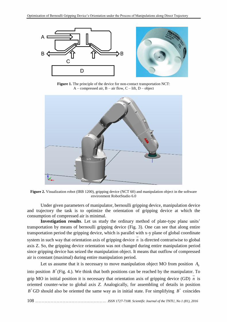
Optimization of Bernoulli Gripping Device’s Orientation under the Process of Manipulations along Direct Trajectory
108 ……………………………………………………………. .ISSN 1727-7108. Scientific Journal of the TNTU, No 1 (81), 2016
Figure 1. The principle of the device for non-contact transportation NCT:
A – compressed air, B – air flow, C – lift, D – object
Figure 2. Visualization robot (IRB 1200), gripping device (NCT 60) and manipulation object in the software
environment RobotStudio 6.0
Under given parameters of manipulator, bernoulli gripping device, manipulation device
and trajectory the task is to optimize the orientation of gripping device at which the
consumption of compressed air is minimal.
Investigation results. Let us study the ordinary method of plate-type plane units’
transportation by means of bernoulli gripping device (Fig. 3). One can see that along entire
transportation period the gripping device, which is parallel with x-y plane of global coordinate
system in such way that orientation axis of gripping device n is directed contrariwise to global
axis Z. So, the gripping device orientation was not changed during entire manipulation period
since gripping device has seized the manipulation object. It means that outflow of compressed
air is constant (maximal) during entire manipulation period.
Let us assume that it is necessary to move manipulation object MO from position 0A
into position *
B (Fig. 4.). We think that both positions can be reached by the manipulator. To
grip MO in initial position it is necessary that orientation axis of gripping device (GD) n is
oriented counter-wise to global axis Z. Analogically, for assembling of details in position *
B GD should also be oriented the same way as in initial state. For simplifying *
B coincides

Roman Mykhailyshyn, Yaroslav Prots’, Volodymyr Savkiv
ISSN 1727-7108. Вісник ТНТУ, № 1 (81), 2016 …………………………………………………………………………………. 109
with з 0B . We are going to plan the motion trajectoty in the form of three rectilinear areas –
10 AA , 11BA , 01BB . Along section 10 AA there is made MO lifting and changing of GD orientation
so it would be optimal in energy consumption during retaining of permanent transportation
along section11BA . Along section 01BB there is made MO sinking down to storage place and
changing of GD orientation to necessary one in final position. The usage of compressed air on
these two sections is sufficient for all types of operations (for example, maximal). Along the
section 11BA we are going to plan MO movement and orientation in such way that energy
consumption of compressed air will be minimal. For this purpose it is necessary to cut the
motion time along this section to minimal one, and GD orientation should cut to minimum the
consumption of compressed air.
Figure 3. Trajectory without reorientation of gripping device while manipulating RobotStudio 6.0 software
It is known that motion during the shortest time under limited power of manipulator
drives is made when the movement on a first half of trajectory 11BA goes on with maximal
acceleration, and with maximal deceleration on the second half of trajectory.
Let us find the optimal GD orientation on the section part where MO moves with
maximal acceleration a .Lifting force of GD is directed counter-wise to GD orientation
axis n . Obviously, orientation axis should be directed in such way so the MO aggregate power
from gravitation and inertia forces would perform the rple of lifting power. Figure 4 shows that
manipulator orientation axis is focused in vector n direction.
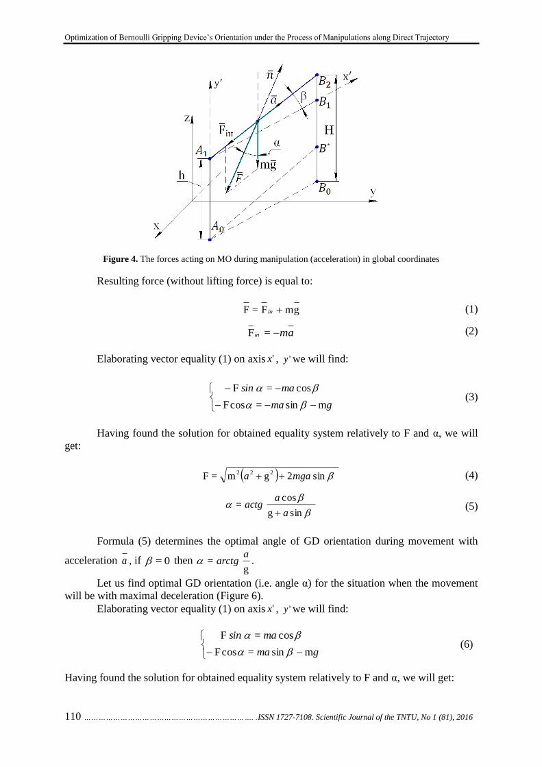
Optimization of Bernoulli Gripping Device’s Orientation under the Process of Manipulations along Direct Trajectory
110 ……………………………………………………………. .ISSN 1727-7108. Scientific Journal of the TNTU, No 1 (81), 2016
Figure 4. The forces acting on MO during manipulation (acceleration) in global coordinates
Resulting force (without lifting force) is equal to:
gmF=F іn (1)
amіn =F (2)
Elaborating vector equality (1) on axis 'x , 'y we will find:
gma
masin
msin=cosF
cos=F
(3)
Having found the solution for obtained equality system relatively to F and α, we will
get:
sin2gm=F222
mgaa (4)
sing
cos=
a
aactg
(5)
Formula (5) determines the optimal angle of GD orientation during movement with
acceleration a , if 0= then g
=a
arctg .
Let us find optimal GD orientation (i.e. angle α) for the situation when the movement
will be with maximal deceleration (Figure 6).
Elaborating vector equality (1) on axis 'x , 'y we will find:
gma
masin
msin=cosF
cos=F
(6)
Having found the solution for obtained equality system relatively to F and α, we will get:
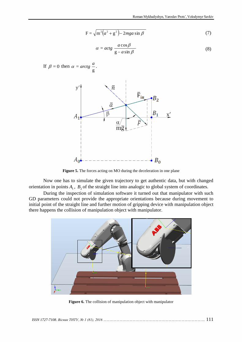
Roman Mykhailyshyn, Yaroslav Prots’, Volodymyr Savkiv
ISSN 1727-7108. Вісник ТНТУ, № 1 (81), 2016 …………………………………………………………………………………. 111
sin2gm=F222
mgaa (7)
sing
cos=
a
aactg
(8)
If 0= then g
=a
arctg .
Figure 5. The forces acting on MO during the deceleration in one plane
Now one has to simulate the given trajectory to get authentic data, but with changed
orientation in points1A ,
2B of the straight line into analogic to global system of coordinates.
During the inspection of simulation software it turned out that manipulator with such
GD parameters could not provide the appropriate orientations because during movement to
initial point of the straight line and further motion of gripping device with manipulation object
there happens the collision of manipulation object with manipulator.
Figure 6. The collision of manipulation object with manipulator

Optimization of Bernoulli Gripping Device’s Orientation under the Process of Manipulations along Direct Trajectory
112 ……………………………………………………………. .ISSN 1727-7108. Scientific Journal of the TNTU, No 1 (81), 2016
That is why we suggested using popular methods that are applied during contour
welding; in particular it was proposed to extend the GD bolting and shift GD axis quadrant
depression �̅� on 30 degrees relatively to final link orientation (Figure 7). Owing to this the
manipulator can easily regenerate any required orientation.
Figure 7. Extension of gripping device with reorientation
Before the simulation one has to mark the main points of reorientation on our rectilinear
trajectory as it is shown on Figure 8. It is also necessary to limit the acceleration along entire
distance by means of function PathAccLim (PathAccLim TRUE \ AccMax:= 2,
TRUE\DecelMax:= 2;).
Figure 8. – Reorientation points location on rectilinear path
Having done the simulation with extender, we will obtain the velocity graph for
manipulation object (Figure 9). As we need the trapezoid velocity profile, one sufficiently has
to limit velocity to point M, which has the slowest speed on path interval 51 TT by means of
function VAR speeddata vmedium (0,44 meters per second).

Roman Mykhailyshyn, Yaroslav Prots’, Volodymyr Savkiv
ISSN 1727-7108. Вісник ТНТУ, № 1 (81), 2016 …………………………………………………………………………………. 113
Figure 9. Velocity of manipulation object
Having limited the velocity to 0,44 meters per second, we obtained the trapezoid
velocity profile (Figure 10).
Figure 10. Graph of trapezoid velocity profile of the manipulation object
Now it is possible to build the graph of gripping device acceleration (Figure 11), which
is necessary to find orientation.
Figure 11. Graph of gripping device acceleration

Optimization of Bernoulli Gripping Device’s Orientation under the Process of Manipulations along Direct Trajectory
114 ……………………………………………………………. .ISSN 1727-7108. Scientific Journal of the TNTU, No 1 (81), 2016
Next step is downloading of GD orientation, particularly the angle between axis’s �̅� and
Z on the section 10TT we download equal to angle α (5) for acceleration on the section
𝑇4𝑇5 – to angle α (8) for deceleration. On the section 21TT we download the change of
orientation from angle α (5) to zero as there is no acceleration on the middle section 𝑇2𝑇3,
orientation stays unchanged and the angle to global system of coordinates is equal to zero. Next
step is downloading of orientation variable on section 𝑇3𝑇4 from zero to angle α (8), which is
optimal on the section with further deceleration. Such orientation is retained on the section
𝑇4𝑇5.
One has to admit from mentioned above that there are two sections 𝑇1𝑇2 і 43TT of
trajectory where we are not sure in secure MO transportation. Perhaps, the most unfavorable
option will occur when in point 1T the acceleration is equal to zero, and the angle here is still
equal to angle α (5) (Figure 12). Let us find the limits for lifting force rate in this case. If there
is no acceleration, then as result of orientation with angle α (5) MO can lose relative balance
and move in S direction. As result, there appears friction force in points of contact between
MO and GD, due to fNF fr , where f friction rate.
Conditions of MO balance are the following
,0cos пFmgN
.0sin mgF fr
Out of the first equation we will find
.cos пFmgN
Then 0=sin=Fcosm mggf п
To provide permanent MO transportation it is necessary to accomplish the condition
,sinFcosm f
mgg п
.cossin
F
fmgабо п (9)
The analogical limits of lifting force rate (9) are on section 𝑇3𝑇4 but the angle is
important (8). For device with m = 0,1 kg, friction rate f = 0,2, angle α = 11.3° we obtain the following
limit:
0294,0F п
It indicates that on sections 𝑇1𝑇2 and 𝑇3𝑇4 the transportation will be permanent and without
applying of lifting force i.e. without supply of GD with compressed air. Under other given
parameters there can appear a necessity in lifting force. It can be done on theses sections with
opening of automatic valve of compressed air supply.
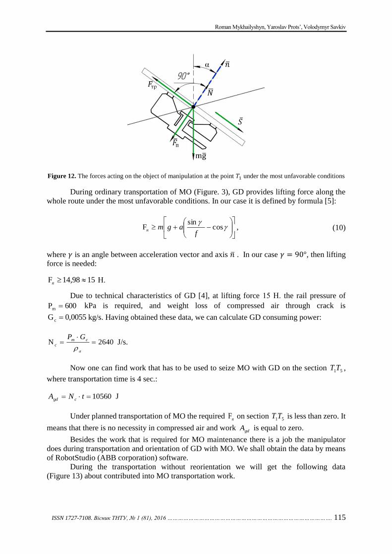
Roman Mykhailyshyn, Yaroslav Prots’, Volodymyr Savkiv
ISSN 1727-7108. Вісник ТНТУ, № 1 (81), 2016 …………………………………………………………………………………. 115
Figure 12. The forces acting on the object of manipulation at the point 𝑇1 under the most unfavorable conditions
During ordinary transportation of MO (Figure. 3), GD provides lifting force along the
whole route under the most unfavorable conditions. In our case it is defined by formula [5]:
cos
sinF
fagmп , (10)
where 𝛾 is an angle between acceleration vector and axis �̅� . In our case 𝛾 = 90°, then lifting
force is needed:
1598,14F п Н.
Due to technical characteristics of GD [4], at lifting force 15 Н. the rail pressure of
600Pm kPa is required, and weight loss of compressed air through crack is
0055,0G c kg/s. Having obtained these data, we can calculate GD consuming power:
2640N
а
cm
c
GP
J/s.
Now one can find work that has to be used to seize MO with GD on the section 51TT ,
where transportation time is 4 sec.:
10560 tNA cgd J
Under planned transportation of MO the required пF on section 51TT is less than zero. It
means that there is no necessity in compressed air and work gdA is equal to zero.
Besides the work that is required for MO maintenance there is a job the manipulator
does during transportation and orientation of GD with MO. We shall obtain the data by means
of RobotStudio (ABB corporation) software.
During the transportation without reorientation we will get the following data
(Figure 13) about contributed into MO transportation work.

Optimization of Bernoulli Gripping Device’s Orientation under the Process of Manipulations along Direct Trajectory
116 ……………………………………………………………. .ISSN 1727-7108. Scientific Journal of the TNTU, No 1 (81), 2016
Figure 13. Work spent on transportation of manipulator of the object manipulation without reorientation
During transportation without reorientation on the section 51TT the MO contributed
140)()( 15 TATAA mmm J of work, and during transportation with reorientation on the
section 51TT the MO contributed 256mA J of work.
Figure 14. Work spent on transportation by manipulator of the object with reorientation
Now we can obtain the aggregate work contributed into MO transportation under two different types of movement.
During transportation without reorientation the aggregate work on section 51TT is
equal to:
107001 mgd AAA J,
and during transportation with reorientation the aggregate work on section 51TT is equal to:
2562 mgd AAA Дж.
Let us find the efficiency coefficient for MO transportation with reorientation:
.402
1 A
A

Roman Mykhailyshyn, Yaroslav Prots’, Volodymyr Savkiv
ISSN 1727-7108. Вісник ТНТУ, № 1 (81), 2016 …………………………………………………………………………………. 117
It means that MO transportation with reorientation allows minimizing the loss of compressed air and decreasing the contributed work into MO transportation along rectilinear trajectory.
Conclusion. There was proposed the optimization of the orientation of the gripping device during the transport of object manipulation on a straight-line trajectory. Transportation using the optimum orientation allows reducing in 40 times the energy consumption comparing to transportation without reorientation. References
1. Mantriota, G. Theoretical model of the grasp with vacuum gripper, Mantriota G., Mechanism and machine Theory. – Taranto, Italy. – N 42. – P. 2 – 17.
2. Mantriota, G. Optimal grasp of vacuum grippers with multiple suction cups, Mantriota G., Mechanism and machine Theory. – Taranto, Italy. – N 42. – P. 18 – 33.
3. Mykhailyshyn M.S. Doslidzhennia umov bezvidryvnoho transportuvannia obiektiv zakhopliu valnymy prystroiamy strumenevoho typu, M. Mykhailyshyn, Ya. Prots, T. Detsyk, Visnyk Ternopilskoho natsionalnoho tekhnichnoho universytetu, 2012, no. 3 (67). – pp. 162 – 172. [in Ukrainian]
4. The official website of the company Bosch Rexroth. Available at: http://www.aventics.com/en/non-contact-transport-system-nct-pk-series/. (accessed 03.03.2016) [In English]
5. Savkiv, V.B. Avtomatyzatsiia protsesiv zavantazhennia obiektiv typu tila obertannia na osnovi strumenevykh zakhopliuiuchykh prystroiv: Diss. kand. tek. nauk. Sevastopol, 1999. [In Ukrainian] Список використаної літератури
1. Mantriota, G. Theoretical model of the grasp with vacuum gripper / Mantriota G. // Mechanism and machine Theory. – Taranto, Italy. – N 42. – P. 2 – 17.
2. Mantriota, G. Optimal grasp of vacuum grippers with multiple suction cups / Mantriota G. // Mechanism and machine Theory. – Taranto, Italy. – N 42. – P. 18 – 33.
3. Михайлишин, М.С. Дослідження умов безвідривного транспортування об’єктів захоплених вальними пристроями струменевого типу [Текст] / М. Михайлишин, Я. Проць, Т. Децик // Вісник Тернопільського національного технічного університету. – 2012. – № 3 (67). – С. 162 – 172.
4. Офіційний сайт фірми Bosch Rexroth [Електронний ресурс]. – Режим доступу: http://www. boschrexroth.com/pneumatics-catalog
5. Савків, В.Б. Автоматизація процесів завантаження об’єктів типу тіла обертання на основі струменевих захоплюючих пристроїв [Текст] / В.Б. Савків.: дис. ... канд. техн. наук.
УДК 621.865.8
ОПТИМІЗАЦІЯ ОРІЄНТАЦІЇ СТРУМИННОГО ЗАХОПЛЮВАЛЬНОГО ПРИСТРОЮ В ПРОЦЕСІ МАНІПУЛЮВАННЯ ПО ПРЯМІЙ ТРАЄКТОРІЇ
Роман Михайлишин; Ярослав Проць; Володимир Савків
Тернопільський національний технічний університет імені Івана Пулюя, Україна
Резюме. Поставлено задачу при заданих параметрах маніпулятора, струминного
захоплювального пристрою, об’єкта маніпулювання і траєкторії визначити оптимальну орієнтацію захоплювального пристрою, при якому споживання стисненого повітря буде мінімальним. Запропоновано розділення прямолінійної траєкторії на 5 ділянок. Визначається оптимальна орієнтація на першій, середній і кінцевій ділянці. На цих ділянках забезпечується безвідривність транспортування об’єкта маніпулювання за допомогою лише сили інерції і сили ваги. На двох проміжних ділянках переорієнтації забезпечується безвідривність транспортування з обмеженням на силу притягання захоплювального пристрою. Наведено розв’язання задачі для конкретного прикладу, при забезпеченні безвідривного транспортування об’єкта маніпулювання на усій траєкторії.
Ключові слова: струминний захоплювальний пристрій, об’єкт маніпулювання, безвідривне транспортування, маніпулятор, орієнтація, промисловий робот.
Отримано 02.03.16

Вісник Тернопільського національного технічного університету
Scientific Journal of the Ternopil National Technical University
2016, № 1 (81)
ISSN 1727-7108. Web: visnyk.tntu.edu.ua
118……………………………………………….………..Corresponding author: Osolinskyy Oleksandr; e-mail:[email protected]
UDC 004.08.01
ERROR OF METHODICAL STUDY AT MEASUREMENT OF
AVERAGE ENERGY CONSUMPTION OF MICROCONTROLLERS
Oleksandr Osolinskyy
The Research Institute for Intelligent Computer Systems, Ternopil National
Economic University, Ternopil, Ukraine
Abstract. The article deals with the comprehensive research of methodical error appearing during
applying of new measurement method for average energy consumption of microcontrollers whole performing
instructions, applications or their fragments. The author revealed that methodical error is rather insignificant, so
the method provides high measurement accuracy and performance in terms of error probability.
Key words: microcontroller, measurement of power consumption, method.
Received 29.12.15
Type Codes
MC – microcontroller;
СS – current stabilizer;
ОB – operation booster;
VS – voltage stabilizer;
SCR – subsystem of current regulation;
SVM – subsystem of voltage measurement.
Problem setting. Built-in computer systems with autonomous power supply have been
widely used lately. Usually, such systems are built on the base of those microcontrollers (MC)
to provide the widest range of methods for economizing of battery and accumulator charge.
One of the relevant tasks of elaboration of such systems is to increase the operation time without
recharging of batteries that requires the corresponding optimization.
According to [1], there exist three main ways to solve the task of increasing of system
operation time in autonomous mode: (i) to increase the capacity of power sources; (ii) to
upgrade the production technology for integrated circuits; (iii) to optimize the power-
consumption software. The two former ways require fundamental research. The third one needs
only the equipment to measure power consumption.
The difficulty of power consumption measurement for MC (as well as for
microprocessors) is evoked with the character of their power consumption. Modern MCs, made
under CMOS (Complementary-symmetry/metal-oxide semiconductor) technology, consume
the current in the form of peaks. These peaks are linked to impulses fronts of clock generator.
Their amplitude exceeds the current constant in tens of times.
Analysis of the latest research and published works. The initial research [2] assumed
the measurement of average energy consumption of MC. Therefore, the built models of MC
power consumption have considerable error (10 per cent and more). Prof. Laopoulos’ group
from University of Salonika (Greece) [3] studied the power consumption of ARM7TDMI
nucleus by means of measurement of instantaneous current of consumption with symmetric
«current mirror». It allowed simultaneous grounding of the digital oscillograph during MC
measurement [3]. The error analysis, made in [1], displayed low accuracy of «current mirror»
due to the change in voltage drop on its transistors during change of MC consumption current.
Into the bargain, the circuit capacitors are cut from MC with «current mirror» (MC power
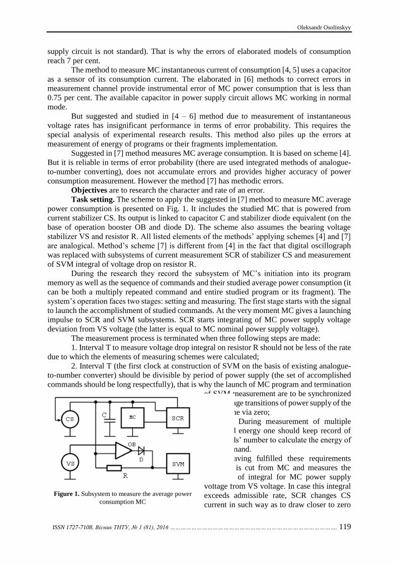
Oleksandr Osolinskyy
ISSN 1727-7108. Вісник ТНТУ, № 1 (81), 2016 …………………………………………………………………………………. 119
supply circuit is not standard). That is why the errors of elaborated models of consumption
reach 7 per cent.
The method to measure MC instantaneous current of consumption [4, 5] uses a capacitor
as a sensor of its consumption current. The elaborated in [6] methods to correct errors in
measurement channel provide instrumental error of MC power consumption that is less than
0.75 per cent. The available capacitor in power supply circuit allows MC working in normal
mode.
But suggested and studied in [4 – 6] method due to measurement of instantaneous
voltage rates has insignificant performance in terms of error probability. This requires the
special analysis of experimental research results. This method also piles up the errors at
measurement of energy of programs or their fragments implementation.
Suggested in [7] method measures MC average consumption. It is based on scheme [4].
But it is reliable in terms of error probability (there are used integrated methods of analogue-
to-number converting), does not accumulate errors and provides higher accuracy of power
consumption measurement. However the method [7] has methodic errors.
Objectives are to research the character and rate of an error.
Task setting. The scheme to apply the suggested in [7] method to measure MC average
power consumption is presented on Fig. 1. It includes the studied MC that is powered from
current stabilizer CS. Its output is linked to capacitor C and stabilizer diode equivalent (on the
base of operation booster OB and diode D). The scheme also assumes the bearing voltage
stabilizer VS and resistor R. All listed elements of the methods’ applying schemes [4] and [7]
are analogical. Method’s scheme [7] is different from [4] in the fact that digital oscillograph
was replaced with subsystems of current measurement SCR of stabilizer CS and measurement
of SVM integral of voltage drop on resistor R.
During the research they record the subsystem of MC’s initiation into its program
memory as well as the sequence of commands and their studied average power consumption (it
can be both a multiply repeated command and entire studied program or its fragment). The
system’s operation faces two stages: setting and measuring. The first stage starts with the signal
to launch the accomplishment of studied commands. At the very moment MC gives a launching
impulse to SCR and SVM subsystems. SCR starts integrating of MC power supply voltage
deviation from VS voltage (the latter is equal to MC nominal power supply voltage).
The measurement process is terminated when three following steps are made:
1. Interval T to measure voltage drop integral on resistor R should not be less of the rate
due to which the elements of measuring schemes were calculated;
2. Interval T (the first clock at construction of SVM on the basis of existing analogue-
to-number converter) should be divisible by period of power supply (the set of accomplished
commands should be long respectfully), that is why the launch of MC program and termination
of SVM measurement are to be synchronized
with voltage transitions of power supply of the
same name via zero;
3. During measurement of multiple
command energy one should keep record of
commands’ number to calculate the energy of
one command.
Having fulfilled these requirements
the SCR is cut from MC and measures the
deviation of integral for MC power supply
voltage from VS voltage. In case this integral
exceeds admissible rate, SCR changes CS
current in such way as to draw closer to zero
Figure 1. Subsystem to measure the average power
consumption MC

Error of Methodical Study at Measurement of Average Energy Consumption of Microcontrollers
120 ……………………………………………………………. .ISSN 1727-7108. Scientific Journal of the TNTU, No 1 (81), 2016
the voltage change in MC circuit during measurement. After this SCR dumps VC and described
setting process is repeated. During a couple of iterations the deviation of MC power supply
voltage from nominal one will not exceed admissible rate. Then the regulation system records
Cs current rate, launches SVM and dumps MC again. SVM starts integrating of voltage drop
on resistor R. After measurement termination (fulfillment of three listed requirements) SCR
again checks up the deviation of MC power supply voltage from VS voltage. If this deviation
exceeds the admissible rate, SCR does not suspend the research process. It again draws CS
current to necessary rate and initiates new measurement cycle. Unless this deviation exceeds
the admissible rate, SCR suspends the research process and launches the calculation of average
rate of energy for a command fulfillment.
The average energy is determined due to the following formula
(1)
where u and i are instantaneous MC voltage and current power rates МК; t – current time ratio;
T – energy measurement period.
Energy balance in switch-board with plugged in CS, MC, C and stabilitron equivalent
can be recorded in strict accordance with Kirchhoff 1st law. Having selected capacity C, one
can succeed in obtaining maximum VC power supply voltage deviations that are rather low
(0,5 – 1 per cent). Then the balance of generated and consumed energy will be recorded as
follows
(2)
where ECS, EMC, EC and ER – according to energy CS (generated, input to switch-board),
MC (consumed, output from switch-board), capacitor C (output from switch-board when
voltage on C grows and comes to switch-board-input, when voltage on C goes down), linked
via OB at MC protection during voltage exceeding of admissible rate on C (consumed, on the
switch-board output).
We neglect the energies consumed by measurement circuits. The change of capacitor
energy конденсатора ∆EC
(3)
where ∆UC is voltage change on the capacitor.
As it was mentioned at the beginning they set current C at first in order to direct MC
voltage deviation integral from initial rate during period T to zero . Then
energy change accumulated by C will go to zero ∆EC→0. That is why the capacitor, which
creates standard work conditions for MC, does not really change the energy balance of
generating / consuming (there are used ceramic capacitors with outflow current). That means
EC can be excluded from (2) and (2) can be re-written as
(4)
ECC in turn does not depend upon MC consuming energy, It can be defined as
(5)
T
t
dtiuE0
RCMCCS EEEE
2/)(2
CC UCE
0)(0
T
REFi dtUu
RCCMK EEE
TIUE CCCHCC

Oleksandr Osolinskyy
ISSN 1727-7108. Вісник ТНТУ, № 1 (81), 2016 …………………………………………………………………………………. 121
When the commands’ set is accomplished with relatively small energy then C voltage
can grow higher than admissible one for this MC. Then OB through D and R «withdraws»
excessive current from MC power supply switch-board. «Withdrawn» energy is taken into
consideration through R by integration of voltage drop for the time period T.
(6)
where uMK, iR are MC ongoing current and
voltage rates through resistor R respectfully.
One has to emphasize that in case
uMK UREF, then (6) can be re-written as
(7)
In this respect (4) can be re-written as
(8)
According to (8) the energy EMK
(consumed by MC) can be defined by means of
voltage UCH (it can be measured by precision
digital volt-meter of direct current), current
струмом ICC (it can measured with precision
digital ampere-meter of direct current)
measurement time T (it can be measured with
digital counter with incoming impulses from
quartz generator with frequency identified by
precision frequency-meter), electrical
resistance R (it can be measured with precision
digital ohmmeter of direct current) and voltage
drop integral on R. Thus, during the experiment
it is necessary to identify only mentioned
integral. For this purpose it is worth to use the
method of two-stroke integrating as one of the
most precise and performing in terms of error
probability during analogue-to-number
transformation [8]. Besides, , so measurement error for
«withdrawn» excessive energy has the minor impact upon measurement result error during MC
energy consumption.
Methodical errors and methods to study them. Methodical errors are intrinsic to
suggested method of measurement of average power of MC energy consumption. The first one
was caused by the change of product integral for instantaneous voltage and current according
T
t
RMK
T
t
RMKR dtR
uudtiuE
00
T
t
RREF
R dtuR
UE
0
T
t
R
CH
CCCHMK dtuR
UTIUE
0
T
t
RREF
VYMREFIREF dtuR
UTIU
0
Set of parameters for research option
∆max, Umax, Umin, Imax,
Imin, n
Cycle under n
Calculation of absolute,
relative, and aggregate
methodical error
Output current
values of
methodological
error
Output the sum
of values the
methodological
error
End cycle under n
end
start
Figure 2. The general algorithm of simulation study

Error of Methodical Study at Measurement of Average Energy Consumption of Microcontrollers
122 ……………………………………………………………. .ISSN 1727-7108. Scientific Journal of the TNTU, No 1 (81), 2016
to (1) on product of nominal values of voltage
and current according to (5). This process can
be described by the equation
(9)
where uj and ij – instantaneous voltage and
current rates on MC power supply contacts
that were measured with system Fig. 1, t –
period of one measurement, T – time of
energy measure.
In case , the voltage changes
on MC are inconsiderable, i.e.
and studied device of
energy consumption is linear, then there is no
methodical error at changes according to (9).
However, MC is semiconducting device so it
has considerable non-linearity. Thus, there is
methodical error due to approximate character
of equation (9). The value of this error is to be
studied. Experimental research of error
dependence from MC power consumption is not reasonable. Every studied MC will reflect only one option of methodical error. That is why t is necessary to apply the imitation modeling method. It will assist in
implementation of all options of methodical error in given framework (even those practically impossible). General algorithm of the research is shown on Fig. 2.
It assumes determination of correlations between absolute and relative rates of methodical current and aggregate errors and number of command implementation cycles or program, non-linearity of energy consumption, maximum voltage and current rates of power supply in accordance with required research conditions. For its implementation it is necessary to build the model of MC power consumption
Model f MC non-linear consumption. The real character of different types MC energy consumption I defined by their technological characteristics. So it is necessary to build up aggregate model of consumption МК IMK (Fig. 3). It includes the minimal consumption current IMIN linear ILIN and non-linear INONLIN current constituents of MC consumption.
(10)
ILIN is defined as ILIN=k∙∆UMK=k∙(UMK-UMIN), where UMK і ∆UMK – current MC voltage and its change; k – coefficient, k=(IMAX-IMIN)/(UMK-UMIN) . INONLIN are defined as
, where A, B – coefficients obtained as result of equation system
solution.
(11)
TIUtiudtiuE REFREF
T
j
jj
T
t
00
)(
TtT
j
0
0)(0
T
REFi dtUu
NONLINLINMINMK IIII
MCMCNONLIN UBUAI 2
MAXMINMAXMINMAX
MINMAXMINMAX
UUBUUA
UUBUUA
2/2/
0
2
2
Figure 3. The generalized model of energy
consumption of MC
Figure 4. Dependence of the relative total average
error of method on number of cycles n performed
commands

Oleksandr Osolinskyy
ISSN 1727-7108. Вісник ТНТУ, № 1 (81), 2016 …………………………………………………………………………………. 123
where ∆MAX – maximal absolute rate of methodical error.
It should be mentioned that for known MC types ∆MAX and its marker are not fixed. Their research is also unknown. So, the model on Fig. 3 assumes ∆MAX of both polarities. Its maximal value during imitation research is given within 10 … 40 per cent.
During the imitation modeling the value ∆UMC is given at random. Thus, different energy consumption of MC is imitated. Methodical error ∆MET grows simultaneously with deviation UMC from UVS. That is why there was selected the equable law of distribution ∆UMC.
Results of methodical error research. Fig. 4 displays the correlation between aggregate average relative methodical error
and number of command cycles n (or
number of rows in the program) as well as non-linearity of MC energy consumption (non-linearity is given to the right side from graphs).
As Fig. 5 shows, considerably drops
simultaneously with n growth. It is explained with the fact that at initial setting of the system (see Fig. 1) the consumption current is set in such way that aggregate MC voltage deviation during given number of cycles n approaches zero. Then values of ∆MET will be both positive
and negative and compensate each other.
Fig. 5 displays the correlations between aggregate relative methodical error
for n = 500 and non-linear type A from non-linearity of MC energy consumption МК в межах 10…40% within 10 … 40 per cent and maximal voltage change on MC from ±10 до ± 50 megavolts (shown right side from graph).
As it show on Fig. 5, in case of non-linearity of consumption current at 40 per cent and
voltage change ± 50 megavolts), . During decrease on non-linearity and voltage
change on MC, decreases considerably.
For non-linearity of B type and under the research conditions the relative methodical error
, as it displayed on Fig. 6, is less. In this case the mutual compensation of errors it acts
more successfully. Conclusions. The research of the methodical error of the proposed method for
measuring the average energy consumption of MC (caused by replacing the integral of product of instantaneous values of voltage and current with the product of the nominal values of voltage and current supply of MC), have shown that it is quite small during multiple performance of an instruction or a program. One should investigate another methodological error that appears due to inequality voltage on the capacitor in the circuit of MC before and after studies (inability to ensure the accurate condition ΔEC → 0) to solve the problem of designing of precision measuring system of MC energy consumption on the basis of the proposed method.
References 1. Borovyi A. Konstantakos V., Kochan V. [et al.] Analysis of CPU's instructions energy consumption device
circuits, Proceedings of the fourth IEEE international workshop on Intelligent Data Acquisition and Advancing Computing Systems (IDAACS’2007), September 9 – 11, 2007, Dortmund, Germany. P. 42 – 47.
2. Tiwari V., Sharad Malik and Wolfe A. Power Analysis of Embedded software: A First Step Towards Software Power Minimization, IEEE Transactions on Very Large Scale Integration (VLSI) Systems, Vol. 2, No. 4, December 1994, pp. 437 – 445.
3. Laopoulos Th., Neofotistos P., Kosmatopoulos C.A., Nikolaidis S. Measurement of current variations for the estimation of software-related power consumption, IEEE Transactions on instrumentation and measurement, Vol. 52 (4), 2003, pp. 1206 – 1212.
MET
MET
MET
%018,0
MET
MET
MET
Figure 5. Dependence of the relative total
average error of method on type A nonlinearity of
energy consumption and maximum voltage
change
Figure 6. Dependence of the relative total
average error of method on type B nonlinearity of
energy consumption and maximum voltage
change

Error of Methodical Study at Measurement of Average Energy Consumption of Microcontrollers
124 ……………………………………………………………. .ISSN 1727-7108. Scientific Journal of the TNTU, No 1 (81), 2016
4. Borovyi A.M., Maikiv I.M., Kochan R.V., Dombrovskyi Z.I., Kochan V.V. Prystrii vymiriuvannia enerhii impulsnykh spozhyvachiv, Zaiavnyk i patentovlasnyk – Borovyi A.M., Maikiv I.M., Kochan R.V., Dombrovskyi Z.I., Kochan V.V. Pat. 90922 Ukrainy, MPK7 G05F 5/00, G01K 17/00., № a200806325; zaiavl. 13.05.08; opubl. 10.06.10, Biul. № 11. [in Ukrainian]
5. Borovyi A., Kochan V., Dombrovskyy Z., Turchenko V., Sachenko A. Device for Measuring Instant Current Values of CPU's Energy Consumption, Proceedings of the fifth IEEE international workshop on Intelligent Data Acquisition and Advancing Computing Systems (IDAACS’2009), September,21 – 23, 2009, Rende, Cosenza, Italy, pp. 126 – 130.
6. Borovyi A. Informatsiino-vymiriuvalna systema doslidzhennia parametriv enerhospozhyvannia mikroprotsesoriv. Diss. kand. tek. nauk. Ternopil, 2012. 266 p. [in Ukrainian]
7. Osolinskyi O.R., Kochan V.V., Dombrovskyi Z.I., Kochan O.V Sposib vymiriuvannia serednoi enerhii impulsnoho spozhyvacha ta prystrii dlia yoho realizatsii, Zaiavnyk i patentovlasnyk Osolinskyi O.R., Kochan V.V., Dombrovskyi Z.I., Kochan O.V. Pat. 110142 Ukrainy, MPK G01R 11/00, G01R 21/00, G05F 5/00., № a2014 03292; zaiavl. 31.03.14; opubl. 25.11.15, Biul. № 22. [in Ukrainian]
8. Kester W. Analogo-cifrovoe preobrazovanie [Pod red. Wolta Kestera]. Moscow, Texnosfera, Publ., 2007. 1016 p. [In Russian] Список використаної літератури
1. Borovyi, A. Analysis of CPU's instructions energy consumption device circuits [Text] / A. Borovyi V. Konstantakos, V. Kochan [et al.] // Proceedings of the fourth IEEE international workshop on Intelligent Data Acquisition and Advancing Computing Systems (IDAACS’2007) / September 9 – 11, 2007, Dortmund, Germany. – Dortmund, 2007. – P. 42 – 47.
2. Tiwari, V. Power Analysis of Embedded software: A First Step Towards Software Power Minimization [Text] / Vivek Tiwari, Sharad Malik and Andrew Wolfe // IEEE Transactions on Very Large Scale Integration (VLSI) Systems. – Vol. 2, No. 4. – December 1994. – P. 437 – 445.
3. Laopoulos, Th. Measurement of current variations for the estimation of software-related power consumption [Text] / Th. Laopoulos, P. Neofotistos, C.A. Kosmatopoulos, S. Nikolaidis // IEEE Transactions on instrumentation and measurement. – Vol. 52 (4). – 2003. – P. 1206 – 1212.
4. Пат. 90922 України, МПК7 G05F 5/00, G01K 17/00. Пристрій вимірювання енергії імпульсних споживачів [Текст] / Боровий А.М., Майків І.М., Кочан Р.В., Домбровський З.І., Кочан В.В. Заявник і патентовласник: Боровий А.М., Майків І.М., Кочан Р.В., Домбровський З.І., Кочан В.В. – № а200806325; заявл. 13.05.08; опубл. 10.06.10, Бюл. № 11.
5. Borovyi, A. Device for Measuring Instant Current Values of CPU's Energy Consumption [Text] / A. Borovyi, V. Kochan, Z. Dombrovskyy, V. Turchenko, A. Sachenko // Proceedings of the fifth IEEE international workshop on Intelligent Data Acquisition and Advancing Computing Systems (IDAACS’2009) / September, 21 – 23, 2009 ,Rende, Cosenza, Italy, – Italy, 2009. – P. 126 – 130.
6. Боровий, А. Інформаційно-вимірювальна система дослідження параметрів енергоспоживання мікропроцесорів: дис. на здобуття наук. ступеня канд. техн. наук: спец. 05.13.05 Комп'ютерні системи та компоненти [Текст] / Андрій Модестович Боровий. – Тернопіль: ТНЕУ, 2012. – 266 с.
7. Пат. 110142 України, МПК G01R 11/00, G01R 21/00, G05F 5/00. Спосіб вимірювання середньої енергії імпульсного споживача та пристрій для його реалізації [Текст] / Осолінський О.Р., Кочан В.В., Домбровський З.І., Кочан О.В.; заявник і патентовласник Осолінський О.Р., Кочан В.В., Домбровський З.І., Кочан О.В.; – № а 2014 03292; заявл. 31.03.14; опубл. 25.11.15, Бюл. № 22.
8. Кестер, Уолт Аналого-цифровое преобразование [Текст] / Уолт Кестер. – М.: Техносфера, 2007. – 1016 с.
УДК 004.08.01
ДОСЛІДЖЕННЯ МЕТОДИЧНОЇ ПОХИБКИ ПРИ ВИМІРЮВАННІ СЕРЕДНЬОГО ЕНЕРГОСПОЖИВАННЯ
МІКРОКОНТРОЛЕРІВ
Олександр Осолінський
Науково-дослідний інститут Інтелектуальних комп’ютерних систем, Тернопільський національний економічний університет,
Тернопіль, Україна Резюме. Розглянуто методичну похибку, що виникає при використанні нового методу
вимірювання середнього енергоспоживання мікроконтролерів під час виконання інструкцій, програм або їх фрагментів. Показано, що методична похибка є достатньо малою, тому метод забезпечує високу точність і завадостійкість вимірювань.
Ключові слова: мікроконтролер, вимірювання енергоспоживання, метод.
Отримано 29.12.15

Вісник Тернопільського національного технічного університету
Scientific Journal of the Ternopil National Technical University
2016, № 1 (81)
ISSN 1727-7108. Web: visnyk.tntu.edu.ua
Corresponding author: Chui Yurii; [email protected] …………………………………………………………………………125
MATHEMATICAL MODELING.
MATHEMATICS
МАТЕМАТИЧНЕ МОДЕЛЮВАННЯ.
МАТЕМАТИКА
UDC 627.324.2/3:532.72
FINITE ELEMENT METHOD IN SPATIAL FILTRATION
CONSOLIDATION PROBLEM WITH THIN SEMI-PERMEABLE
INCLUSIONS UNDER THE INFLUENCE OF THE HEAT AND SALT
TRANSFER
Yurii Chui; Petro Martynyuk
National University of Water Management and Natural Resources Use,
Rivne, Ukraine
Summary. Mathematical model of filtration consolidation of soils, taking into account available there
thin semi-permeable inclusions in three-dimensional case, has been constructed. The finite element method was
used for numerical solution of three-dimensional problem. A number of numerical experiments has been done and
the influence of the heat and salt transfer and semi-permeable inclusions on the distribution of the pressures in
soil massifs has been shown.
Key words: filtration consolidation, matching conditions, semi-permeable inclusion, finite element
method.
Received 11.01.16
Introduction. Soil massifs can contain heterogeneity under natural conditions [7, 15,
16]. Semi-permeable inclusions, through properties of the materials, from which they are
composed, are free to pass water and partly to pass various chemicals dissolved in water. This
kind of inclusions has properties of semi-permeable membranes [17].
Availability of semi-permeable properties in the clays is explained by the phenomenon
of chemical osmosis, in other words, by the dissolvent flow through semi-permeable partition,
which is free to pass molecules of dissolvent and blocks molecules of dissolved substance [6].
Osmosis appears at micro and macro levels in soils. Availability of osmosis flow is like
filtration anomaly, so far as osmotic flow, depending on direction, can speed up diffusion and
filtration or prevent them.
The phenomena of internal and external osmosis, under the influence of which double
electrical layer of particles, that serves as a semi-permeable membrane and correspondingly has
their properties, were investigated in the article [13]. Due to this, there is the necessity of
forecast amendment of engineering structures based on the soils with semi-permeable
inclusions.

Finite Element Method in Spatial Filtration Consolidation Problem with Thin Semi-permeable Inclusions under the Influence
of the Heat and Salt Transfer
126 ……………………………………………………………. .ISSN 1727-7108. Scientific Journal of the TNTU, No 1 (81), 2016
The actuality of the research of consolidation processes in multivendor environment is
explained by the necessity of defining stability of industrial, civil, hydro-technical structures
built on heterogeneous soil layers [10].
Consolidation of heterogeneous soil foundation during vertical drainage establishment
was investigated in [11]. Mathematical model was built in three-dimensional case. The solution
of corresponding boundary problem was shown in the form of combination of Bessel functions.
Fractional differential mathematical model for investigation of locally unbalanced geo-
migration processes, including chemical osmosis and ultra filtration, and mathematical
modeling for consolidation dynamics of double-layer geoporous massif located on
impenetrable base non-equilibrium in time, were constructed in [1, 2].
Works of the following scholars as I. Serhiyenko, V. Skopetskyy, V. Deyneka,
A. Vlasyuk, Th. J.S. Keijzer, M. Petryk were dedicated to processes of heterogeneous porous
medium [7, 14 – 16, 17, 18]. Particularly, mathematical models for filtration soil consolidation
under the influence of the heat and salt transfer with the availability of thin inclusions which
have characteristics of semi-permeable membranes were constructed in [4]. However, only one-
dimensional case of problem was examined there.
There were a great number of damages because of non-uniform settings of big buildings
built in the first half of the last century, when only general theoretical principles of filtration
consolidation of clay soils were known. For example, there was a collapse of Transcona elevator
in Canada, which was located on lake clay deposits with a depth
of 9 m [8].
Nowadays, the whole range of examples emphasizes the actuality of investigations of
filtration consolidation processes, particularly taking into consideration salt transfer under
anisothermic conditions, – while building and operation of Rivne, Zaporizhzhya, Balakiv
atomic power stations, the necessity arose for solving problems, concerning non-uniform soil
deformation of bases of constructions. In particular, while building Balakiv atomic power
station, counter-loads of thousand tons (hinged vessels filled with water), the weight of which
had to be always corrected, were used to avoid big slopes of reactor blocks [12].
The special attention should be paid to three-dimensional case. It shows the influence
of different factors the most completely and equally, and study of three-dimensional case gives
a possibility to take into consideration the area of consolidation, and to set a location of thin
clay semi-permeable inclusions in sand soils more precisely.
Research objective is to investigate processes of consolidation of soil with available
there semi-permeable inclusions in three-dimensional case and the influence of the heat and salt
transfer on the given processes in soil.
Problem statement and its mathematical model. Considering the given area Ω ,
consisting of homogeneous soil and thin semi-permeable inclusions, without loss of generality,
we will suppose that such inclusion is one ( * Fig. 1).
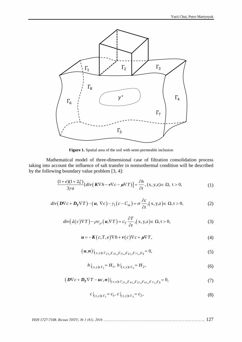
Yurii Chui, Petro Martynyuk
ISSN 1727-7108. Вісник ТНТУ, № 1 (81), 2016 …………………………………………………………………………………. 127
Figure 1. Spatial area of the soil with semi-permeable inclusion
Mathematical model of three-dimensional case of filtration consolidation process
taking into account the influence of salt transfer in nonisothermal condition will be described
by the following boundary value problem [3, 4]:
(1 )(1 2 )
[ ) , (x, y,z) Ω, t 0,3
e hdiv h c T
a t
K ν μ (1)
1, , x, y,z Ω, t 0,m
cdiv c T c c C
t
TD D u (2)
, , x, y,z Ω, t 0,T
Tdiv c T c T c
t
λ u (3)
, , ,c T e h c c T u K ν μ (4)
2 4 5 6 7 8, Γ Γ Γ Γ Γ Γ, | 0,
x y
u n (5)
1 31 2, Γ , Γ| , | ,
x y x yh H h H
(6)
2 4 5 6 7 8, Γ Γ Γ Γ Γ Γ, | 0,
x yc T c
TD D u n (7)
1 31 2, Γ , Γ| , | ,
x y x yc c c c
(8)
Γ5
Γ4 Γ6
Γ1 Γ3
𝛾∗
Γ2
Γ7
Γ8

Finite Element Method in Spatial Filtration Consolidation Problem with Thin Semi-permeable Inclusions under the Influence
of the Heat and Salt Transfer
128 ……………………………………………………………. .ISSN 1727-7108. Scientific Journal of the TNTU, No 1 (81), 2016
2 7 84 5 6, Γ Γ Γ Γ Γ Γ( , ) | 0,
x yc T c T
λ u n (9)
1 31 2, Γ , Γ| , | ,
x y x yT T T T
(10)
* * *
**
, , , , 0,k
h h c c T T x y td d d
u n (11)
**
***
, 1 , , , , 0,TDDc c T T x y t
d d
cq n u n (12)
*
* **
, , , , , 0,c u n T T T x y td
Tq n (13)
* * *, | 0, , | 0, , | 0, 0,t
c Tu n q n q n (14)
, ,c c T c T c T c T Tq u D D q u λ (15)
0 0 0, , , 0 , , , , , , 0 , , , , , , 0 , , ,h x y z h x y z c x y z c x y z T x y z T x y z
( , , ) ,x y x
(16)
where h – pressure; c – concentration; T – temperature; ( , , )c T eK K – filtration coefficient;
ν – chemical osmosis coefficient; μ – thermal osmosis coefficient; – specific gravity of
pore liquid; e – coefficient of soil porosity; – coefficient of lateral soil pressure;
a – coefficient of soil constriction; u – vector of filtration speed; D – coefficient of convective
diffusion; TD – coefficient of thermal diffusion; mC – concentration of soil saturation limit;
1 – coefficient of mass-transfer rate; – soil porosity; λ – coefficient of effective damp soil
thermal conductivity; – density of pore solution; c – specific heat of pore solution;
Tc – soil volumetric heat; d – thickness of semi-permeable inclusion; *
k
, * ,
* , *
D ,
*
TD
, * – characteristics of semi-permeable inclusion * ; – degree of ideality of semi-
permeable inclusion, 0 1 ; n – directed vector of directional cosine of the normal before
semi-permeable inclusion; 0 , ,h x y z , 0 , ,c x y z , 0 , ,T x y z , 1H , 2H , 1c , 2c , 1T , 2T –
specified functions; 71 2 3 4 5 6 8Γ Γ Γ Γ Γ Γ Γ Γ Γ – area border Ω .
Numerical solution of boundary value problem received with the help of finite
element method (FEM). Considering 0H – as space of vector-functions
1 2 3, , ( , , ; , , ; , , )s x y z s x y z s x y z s x y z , each element 1 2 3, , , , , , , ,s x y z s x y z s x y z
of which in area Ω (except limit points Γ and inclusions * ) belong to Sobolyev space
12 (Ω)W , besides that 1 2 3, , , , , , , ,s x y z s x y z s x y z obtain zero meaning in those parts of
area Ω , where correspondingly for the next functions , , , , , , , , , , ,h x y z t c x y z t T x y z t ,
limit conditions of the first kind are established.

Yurii Chui, Petro Martynyuk
ISSN 1727-7108. Вісник ТНТУ, № 1 (81), 2016 …………………………………………………………………………………. 129
Multiplying equations (1) – (3) and each of initial conditions (16) by functions
1 2 3 0( , , ; , , ; , , )s x y z s x y z s x y z H and having integrated received equations in area Ω ,
after use of the Gauss-Ostrogradsky formula, taking into account limit conditions (5) – (10) and
matching conditions (11) – (14), we will receive
1
Ω Ω
1 1 2( , ,
3
ehs dxdydz c T e h c c T
t a
K ν μ
* * *
*
1 1
1( )[ ] ) 0,s dxdydz k h c T s dГ
d
(17)
1 0 1
Ω Ω
, , ,0 , , ( , , ) , , ,h x y z s x y z dxdydz h x y z s x y z dxdydz (18)
2 2 2
Ω Ω Ω
( , ) ( , )c
s dxdydz c s dxdydz T s dxdydzt
TD D
**
*
2 1 2
Ω Ω
, 1 (( TDDc s dxdydz cs dxdy c T
d d
u
* *2 2 1 2
Ω
) ]), , [ ,mc s cs dГ C s dxdydz
u n u n
(19)
2 0 2
Ω Ω
, , , 0 , , ( , , ) , , ,c x y z s x y z dxdydz c x y z s x y z dxdydz (20)
*
*
3 3
Ω Ω
1, ((T
Tc s dxdydz c T s dxdydz T c
t d d
λ
* *3 3 3
Ω
, , [ ])) , 0,T s c Ts dГ c T s dxdydz
u n u n u
(21)
3 0 3
Ω Ω
, , , 0 , , ( , , ) , , .T x y z s x y z dxdydz T x y z s x y z dxdydz (22)
We will seek approximate generalized solution in the following equation
1 2
1 1
, , , ; , , , ; , , , (ˆ , , ; , ,ˆ ;ˆn n
i i j j
i j
h x y z t c x y z t T x y z t a t N x y z b t N x y z
3
1
, , ),n
S s
s
r t N x y z
де 31 2;0;0 , 0; ;0 , 0;0; ,i j kN N N
i j kN N N
, ,1i n 1, , j n 1,k n – basic vector-functions of finite-dimensional subspace 0 0M H ,
which are discontinuous on inclusion [5, 10, 11].
To solve the problem with the help of finite element method, we will discretise area Ω
into tetrahedrons with double numeration of points placed on inclusion. Substituting form of
approximate solution in equations (17) – (22), we will receive Cauchy problem for the system
of non-linear differential equations relating to vector ( ; ; ( ))t t t tU A B R
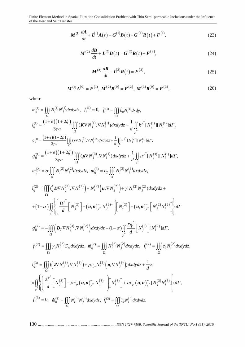
Finite Element Method in Spatial Filtration Consolidation Problem with Thin Semi-permeable Inclusions under the Influence
of the Heat and Salt Transfer
130 ……………………………………………………………. .ISSN 1727-7108. Scientific Journal of the TNTU, No 1 (81), 2016
1 1 1 1(1),
dt t t
dt
'AM L A G B G R F (23)
2 2 2(2),
dt t
dt
BM L B G R F (24)
3 3(3),
dt
dt
RM L R F (25)
0 1 2 0 2 3 0 3(1)
, , , M A F M B F M R F (26)
where
1 1(1)
Ω
,ij i jm N N dxdydz (1)
0,if (1) (1)0
Ω
,i if h N dxdy
*
*
1 1(1) (1) (1)1 1 2 1( , ) [ ][ ] ,
3ij j i j i
el N N dxdydz k N N dГ
a d
K
*
*
2 1(1) (2) (1)1 1 2 1( , ) [ ][ ] ,
3ij j i j i
eg N N dxdydz N N dГ
a d
ν
*
*
3 1'(1) (3) (1)1 1 2 1( , ) [ ][ ] ,
3ij j i j i
eg N N dxdydz N N dГ
a d
μ
2 2(2)
Ω
,ij i jm N N dxdydz 3 3(3)
,ij T i jm c N N dxdydz
*
* *
*
2 2 2 2(2) (2) (2)1
2 2 2 2 2
( , , )
1 , ,
ij j i i j i j
j j i j i
l N N N N N N dxdydz
DN N N N N dГ
d
D u
u n u n
*
*
3 2 3 2(2), (1 ) [ ] ,T
ij j i j i
Dg N N dxdydz N N dГ
d
TD
2(2)1 ,i i mf N C dxdydz
2 2(2)
,ij i jm N N dxdydz
2(2)
0 ,i if c N dxdydz
*
* *
*
3 3 3 3(3)
3 3 3 3 3
1( , , )
, , [ ] ,
ij j i i j
j j i j i
l N N c N N dxdydzd
N c N N c N N dГd
λ u
u n u n
(3)0, if 3 3(3)
, ij i jm N N dxdydz
3(3)
0 .i if T N dxdydz

Yurii Chui, Petro Martynyuk
ISSN 1727-7108. Вісник ТНТУ, № 1 (81), 2016 …………………………………………………………………………………. 131
We will receive approximate solution of the system of non-linear differential equations
(23) – (25) with the help of the Crank-Nicolson scheme [9]
1
3 3 1/2 1/ (32 1/2 2 1)1/ /2( ) , , ,( )
j jj j j j j
R R
M L A B R R F
1
2 2 1/2 1/2 1/2 1/2 2 1/ (2)2 1/2( ) ( , , ) ,
j jj j j j j j
B B
M L A B R B G R F+
1
1 1 1/2 1/2 1/2 1 1/ ( )2 /1 1 2( ) ( , ) ,
j jj j j j j
A A
M L B R A F+G B
where 0
1
t
m , 10,1,2,..., 1,j m ( )j
A – value of elements at ,t j 10, 1;j m
( 1/2) ( 1) ( )1( )
2
j j j A A A . Another vectors and matrices have similar notations.
Received scheme is non-linear relatively to required functions on time layers
1( 1), 0, 1j j m . That is why, for its solution, it is necessary to use iterated methods. To
avoid this, the scheme predicator-corrector can be used [15].
Results of numeral experiments. Three-dimensional problem of filtration
consolidation of soil in the basis of hydro-technical construction taking into account the heat
and salt transfer with the following basic data was investigated:
0.7e , 0.75 , 26
5.12 10 мaн
, 4 1
10 доба , 5
2 10 q м ,
5511 22 2.8 10 м
кг доба
, 26
11 22 2.8 10 мград доба
,
2
11 22 0.02 мD Dдоба
,
*7
6 10 мkдоба
,
* 5510 м
кг доба
,
* 2610 м
град доба
, 0.2 d м ,
350 mгC
літр ,
* 20.0002 мD
доба , 0.1 ,
31100 кгм
, 4.2 кДж
cкг град
,
32137 TкДж
cм град
, 11 0 доба , 108
кДжм град доба
, *
108 кДж
м град доба
,
1 8 H м , 2 2 H м , 1 350 гс
літр , 1 30 T ℃ ,
0 5 гслітр
, 1 20 T ℃ , 10 діб .
(м-m, кг-kg, град-grade, доба-day, діб-days, літр-liter, кДж-kJ) Experimental
dependencies for filtration coefficient and their approximation were taken from work [5].
Soil area is right-angled parallelepiped 10 10 10м м м . Area of load application q is
located between right lines 2.9x м і 7.1x м in plane 0z .
Semi-permeable inclusion is located in the depth of 5 m. It is in the form of rectangle
with tops (3;3) , (3; 7) , (8; 7) , (8;3) .

Finite Element Method in Spatial Filtration Consolidation Problem with Thin Semi-permeable Inclusions under the Influence
of the Heat and Salt Transfer
132 ……………………………………………………………. .ISSN 1727-7108. Scientific Journal of the TNTU, No 1 (81), 2016
Figure 2. Distribution of the pressures when t=720 days with taking into account heat and salt transfer
Figure 3. Distribution of the pressures when t=720 days without taking into account heat and salt transfer
Table № 1.
Jumps of pressure on inclusion taking into account the heat and salt transfer (dimension is defined by meters)
x y z t=30
days
t=180
days
t=360
days
t=720
days
t=1080
days
t=1440
days
3 5 5 0,2152 -0,6366 -0,3934 0,0359 0,2196 0,2920
4,643 5,893 5 0,2275 -1,3838 -0,9825 -0,1550 0,2071 0,3487
4,000 5,000 5 0,3130 -1,2567 -0,8491 -0,0513 0,2932 0,4273
7,274 6,310 5 -0,1634 -1,2844 -0,9507 -0,3467 -0,0744 0,0359
5,714 6,786 5 0,0852 -1,2145 -0,8825 -0,2317 0,0565 0,1698
5 5 5 0,2893 -1,6253 -1,1573 -0,2084 0,2063 0,3681
7,786 5,714 5 -0,2860 -1,2546 -0,9377 -0,3673 -0,1076 -0,0007
8,000 5,000 5 -0,2702 -1,0523 -0,7867 -0,3129 -0,0971 -0,0079
4,286 3,214 5 0,2678 -0,8096 -0,5465 -0,0290 0,1964 0,2830
4,643 4,107 5 0,2960 -1,3766 -0,9612 -0,1286 0,2350 0,3765
6,381 4,048 5 -0,0007 -1,5514 -1,1363 -0,3494 0,0009 0,1407
7,238 3,571 5 -0,1883 -1,0700 -0,7912 -0,2907 -0,0637 0,0289

Yurii Chui, Petro Martynyuk
ISSN 1727-7108. Вісник ТНТУ, № 1 (81), 2016 …………………………………………………………………………………. 133
Table № 2.
Jumps of pressure on inclusion without taking into account the heat and salt transfer
(dimension isdefined by meters)
x y z t=30 days t=180
days
t=360
days
t=720
days
t=1440
days
3 5 5 0,2316 -0,0170 -0,2329 -0,3005 -0,2203
4,643 5,893 5 0,2456 -0,1672 -0,6451 -0,8011 -0,6495
4,000 5,000 5 0,3359 -0,0941 -0,5349 -0,6750 -0,5284
7,274 6,310 5 -0,1379 -0,4028 -0,6964 -0,7901 -0,6763
5,714 6,786 5 0,1046 -0,2713 -0,6289 -0,7440 -0,6219
5 5 5 0,3098 -0,2185 -0,7534 -0,9289 -0,7572
7,786 5,714 5 -0,2554 -0,4237 -0,6903 -0,7741 -0,6655
8,000 5,000 5 -0,2433 -0,3595 -0,5777 -0,6461 -0,5561
4,286 3,214 5 0,2872 -0,0784 -0,3657 -0,4557 -0,3576
4,643 4,107 5 0,3181 -0,1568 -0,6284 -0,7822 -0,6291
6,381 4,048 5 0,0247 -0,3933 -0,8021 -0,9342 -0,7886
7,238 3,571 5 -0,1595 -0,3425 -0,5852 -0,6608 -0,5648
Considering the stated above results (Fig. 2, 3), we can see how the heat and salt transfer
influence the distribution of the pressures in the soil. Taking into account the given processes,
filtration consolidation takes place nearly in one and a half times more rapid than while without
taking into account the heat and salt transfer.
As we can see in Table 1, jump of the pressures is observed on semi-permeable
inclusion, besides almost at all points it is negative and then it becomes positive, (taking into
account the heat and salt transfer at time layer t = 1080 days). Without considering the heat and
salt transfer, the change of jump of the pressure takes place more slowly without change of a
sign.
Conclusions. The model of filtration consolidation of soils with semi-permeable
inclusions in three-dimensional case has been constructed. The influence of the heat and salt
transfer, taking into account the level of ideality of semi-permeable inclusion, on the
distributions of pressures has been shown. Jump of the pressure on the inclusion was found and
the dynamics of its change was investigated. A number of numerical experiments has been
conducted.
Theoretical investigations of quality characteristics of obtained numerical solutions
are planned to be done in future.
References
1. Blagoveshhenskaya T.Yu., Bulavackij V.M., Gladkij A.V. Analiticheskoe reshenie zadachi
matematicheskogo modelirovaniya odnogo lokal'no-neravnovesnogo izotermicheskogo geomigracionnogo
processa, Komp'yuternaya matematika, 2013, No 1, p. 13 – 20. [In Russian]
2. Blagoveshhenskaya T.Yu., Bulavackij V.M. Zadacha modelirovaniya drobno-differencial'noj
konsolidacionnoj dinamiki dvuxslojnoj geoporistoj sredy, Komp'yuternaya matematika, 2014, No 1, p. 3 – 9.
[In Russian]
3. Vlasiuk A.P., Martyniuk P.M. Matematychne modeliuvannia konsolidatsii gruntiv v protsesi filtratsii
solovykh rozchyniv, Rivne: Vyd-vo UDUVHP, 2004, 211 p. [in Ukrainian]
4. Vlasiuk A.P., Martyniuk P.M. Matematychne modeliuvannia konsolidatsii gruntiv pry filtratsii solovykh
rozchyniv v neizotermichnykh umovakh, Rivne: NUVHP, 2008, 416 p. [in Ukrainian]

Finite Element Method in Spatial Filtration Consolidation Problem with Thin Semi-permeable Inclusions under the Influence
of the Heat and Salt Transfer
134 ……………………………………………………………. .ISSN 1727-7108. Scientific Journal of the TNTU, No 1 (81), 2016
5. Vlasiuk A.P., Martyniuk P.M., Koziuk O.V. Eksperymentalni zalezhnosti kharakterystyk gruntiv vid
vplyvu tekhnohennykh faktoriv ta yikh obrobka za metodom naimenshykh kvadrativ, Visnyk Natsionalnoho
universytetu vodnoho hospodarstva ta pryrodokorystuvannia., 2007, Vol. 1 (37), p. 268 – 281. [in Ukrainian]
6. Gruntovedenie, pod. red. V.T. Trofimova, M.:Izd-vo MGU, 2005, 1024 p. [In Russian]
7. Dejneka V.S., Sergienko I.V., Skopeckij V.V. Modeli i metody resheniya zadach s usloviyami
sopryazheniya, Kiev: Nauk. dumka, 1998, 614 p. [In Russian]
8. Zhilenkov V.N., Belkova I.N. Sposob regulirovaniya osadok tyazhelyx sooruzhenij, fundiruemyx v
vodonosnoj tolshhe slabopronicaemyx gruntov, Izvestiya VNIIG imeni B. E. Vedeneeva, 2009, Vol. 256,
p. 10 – 22. [In Russian]
9. Zenkevich O. Konechnye e'lementy i approksimaciya, K. Morgan, M.: Mir, 1986, 318 c. [In Russian]
10. Ivanov P.L. Grunty i osnovaniya gidrotexnicheskix sooruzhenij. Mexanika gruntov, Moskva: Vyssh.
Shkola, 1985, 352 p. [In Russian]
11. Konsolidaciya neodnorodnyx gruntovyx osnovanij pri ustrojstve vertikal'nyx dren, A.D. Dasibekov,
A.A. Yunusov, O.B. Kambarova, A.M. Polatbek, Mezhdunarodnyj zhurnal prikladnyx i fundamental'nyx
issledovanij, 2014, No8, S. 13 – 17. [In Russian]
12. Opyt kontrolya i korrektirovki naklona zdanij reaktornyx otdelenij Balakovskoj AE'S, A.G. Zalizskij,
V.I. Skrypnikov, Yu.V. Tinyakov i dr., Atomnye e'lektricheskie stancii, 1991, Vol. 12. p. 12 – 27. [In Russian]
13. Osipov V.I. Fiziko-ximicheskaya teoriya e'ffektivnyx napryazhenij v gruntax, Gruntovedenieyu, 2013,
No 2, p. 3 – 34. [In Russian]
14. Petryk M.R., Deineka V.S., Vorobiiev Ye.I., Matematychne modeliuvannia filtratsiinoi konsolidatsii v
neodnoridnykh bahatokomponentnykh tsylindrychnykh dyspersnykh mikroporystykh seredovyshchakh,
Kompiuternaia matematyka, 2013, No 1, s. 37 – 45. [in Ukrainian]
15. Sergienko I.V., Skopeckij V.V., Dejneka V.S. Matematicheskoe modelirovanie i issledovanie procesov v
neodnorodnіx sredax, Kiev: Nauk. dumka, 1991, 432 p. [in Ukrainian]
16. Serhiienko I.V., Deineka V.S. Informatsiina tekhnolohiia doslidzhennia protsesiv v bahatokomponentnykh
hruntovykh seredovyshchakh ta optymalne keruvannia yikh stanamy, Nauka ta innovatsii, 2005, Vol. 1., No 3,
p. 34 – 50. [in Ukrainian]
17. Keijzer Th.J.S. Chemical osmosisin natural clayey materials, Geologica Ultraiectina, 2000, No 196, 152 p.
18. Skopetskii V.V., Volokh L.V. Mathematical modeling of filtration consolidation of water-saturated
randomly inhomogeneous soil masses, Cybernetics and System Analysis, 2008, Vol. 44, No. 1, p. 68 – 77.
Список використаної літератури
1. Благовещенская, Т.Ю. Аналитическое решение задачи математического моделирования одного
локально-неравновесного изотермического геомиграционного процесса [Текст] / Т.Ю. Благовещенская,
В.М. Булавацкий, А.В. Гладкий // Компьютерная математика. – 2013. – № 1. – С. 13 – 20.
2. Благовещенская, Т.Ю. Задача моделирования дробно-дифференциальной консолидационной
динамики двухслойной геопористой среды [Текст] / Т.Ю. Благовещенская, В.М. Булавацкий //
Компьютерная математика. – 2014. – № 1. – С. 3 – 9.
3. Власюк, А.П. Математичне моделювання консолідації ґрунтів у процесі фільтрації сольових
розчинів [Текст] / А.П. Власюк, П.М. Мартинюк. – Рівне: Вид-во УДУВГП, 2004. – 211 с.
4. Власюк, А.П. Математичне моделювання консолідації ґрунтів при фільтрації сольових розчинів у
неізотермічних умовах [Текст] / А.П. Власюк, П.М. Мартинюк. – Рівне: НУВГП, 2008. – 416 с.
5. Власюк, А.П. Експериментальні залежності характеристик ґрунтів від впливу техногенних факторів
та їх обробка за методом найменших квадратів [Текст] / А.П. Власюк, П.М. Мартинюк, О.В. Козюк //
Вісник Національного університету водного господарства та природокористування. –
2007. – Вип. 1 (37). – С. 268 – 281.
6. Грунтоведение; под. ред. В.Т. Трофимова. – М.:Изд-во МГУ, 2005. – 1024 с.
7. Дейнека, В.С. Модели и методы решения задач с условиями сопряжения [Текст] / В.С. Дейнека,
И.В. Сергиенко, В.В. Скопецкий. – Киев: Наук. думка, 1998. – 614 с.
8. Жиленков, В.Н. Способ регулирования осадок тяжелых сооружений, фундируемых в водоносной
толще слабопроницаемых грунтов [Текст] / В.Н. Жиленков, И.Н. Белкова // Известия ВНИИГ
имени Б.Е. Веденеева. – 2009. – Том 256. – С. 10 – 22.
9. Зенкевич, О. Конечные элементы и аппроксимация [Текст] / О. Зенкевич, К. Морган. – М.: Мир,
1986. –318 c.

Yurii Chui, Petro Martynyuk
ISSN 1727-7108. Вісник ТНТУ, № 1 (81), 2016 …………………………………………………………………………………. 135
10. Иванов, П.Л. Грунты и основания гидротехнических сооружений. Механика грунтов [Текст] /
П.Л. Иванов. – Москва: Высш. школа, 1985. – 352 с.
11. Консолидация неоднородных грунтовых оснований при устройстве вертикальных дрен [Текст] /
А.Д. Дасибеков, А.А. Юнусов, О.Б. Камбарова, А.М. Полатбек // Международный журнал прикладных и
фундаментальных исследований. – 2014. – № 8. – С. 13 – 17.
12. Опыт контроля и корректировки наклона зданий реакторных отделений Балаковской АЭС [Текст] /
А.Г. Зализский, В.И. Скрыпников, Ю.В. Тиняков и др. // Атомные электрические станции. – 1991. –
Вып. 12. – С. 12 – 27.
13. Осипов, В.И. Физико-химическая теория эффективных напряжений в грунтах [Текст] / В.И. Осипов
// Грунтоведениею – 2013. – № 2. – С. 3 – 34.
14. Петрик, М.Р. Математичне моделювання фільтраційної консолідації в неоднорідних
багатокомпонентних циліндричних дисперсних мікропористих середовищах [Текст] / М.Р. Петрик,
В.С. Дейнека, Є.І. Воробієв // Компьютерная математика. – 2013. – №1. – C. 37 – 45.
15. Сергиенко, И.В. Математическое моделирование и исследование процесов в неоднородных средах
[Текст] / И.В. Сергиенко, В.В. Скопецкий, В.С. Дейнека. – Киев: Наук. думка, 1991. – 432 с.
16. Сергієнко, І.В. Інформаційна технологія дослідження процесів у багатокомпонентних грунтових
середовищах та оптимальне керування їх станами [Текст] / І.В. Сергієнко, В.С. Дейнека // Наука та
інновації. – 2005. – Т. 1, № 3. – С. 34 – 50.
17. Keijzer Th.J.S. Chemical osmosisin natural clayey materials / Th.J.S. Keijzer // Geologica Ultraiectina. –
2000. – № 196. – 152 p.
18. Skopetskii V.V. Mathematical modeling of filtration consolidation of water-saturated randomly
inhomogeneous soil masses / V.V. Skopetskii, L.V. Volokh // Cybernetics and System Analysis. – 2008. – Vol. 44,
No. 1. – Р. 68 – 77.
УДК 627.324.2/3:532.72
МЕТОД СКІНЧЕННИХ ЕЛЕМЕНТІВ У ПРОСТОРОВІЙ ЗАДАЧІ
ФІЛЬТРАЦІЙНОЇ КОНСОЛІДАЦІЇ ҐРУНТІВ З ТОНКИМИ
НАПІВПРОНИКНИМИ ВКЛЮЧЕННЯМИ В УМОВАХ ВПЛИВУ
ТЕПЛОСОЛЕПЕРЕНЕСЕННЯ
Юрій Чуй; Петро Мартинюк
Національний університет водного господарства та
природокористування, Рівне, Україна
Резюме. Сформовано математичну модель фільтраційної консолідації ґрунтів з урахуванням
наявних там тонких напівпроникних включень у просторовому випадку. Для чисельного розв’язання
тривимірної задачі використано метод скінченних елементів. Проведено ряд чисельних експериментів та
показано вплив теплосолеперенесення і напівпроникних включень на розподіл напорів у ґрунтових пластах.
Ключові слова: фільтраційна консолідація, умови спряження, напівпроникне включення, метод
скінченних елементів.
Отримано 11.01.16

Вісник Тернопільського національного технічного університету
Scientific Journal of the Ternopil National Technical University
2016, № 1 (81)
ISSN 1727-7108. Web: visnyk.tntu.edu.ua
136………………………………………….…………….. Corresponding author: Solyar Tetyana; e-mail: [email protected]
UDC 539.3
WAYS TO IMPROVE FOURIER SERIES CONVERGENCE AND ITS
APPLICATION FOR LAPLACE NUMERICAL INVERSION
Тetyana Solyar
Pidstryhach Institute for Applied Problems of Mechanics and Mathematics,
National Academy of Sciences of Ukraine, Lviv, Ukraine
Summary. The solution of a wide class of the problems of mathematical physics can be obtained in the
form of Fourier series. When considering the problems, concerned with study of the localized actions, the quick-
changing solutions are obtained, in this connection the series converge slowly. To solve complex problems the
Fourier series method is used jointly with other approaches, in particular, when using in addition the boundary
element method the series coefficients are determined by solving one- and two-dimensional integral equations that
demands a large amount of calculations. The series coefficients are determined with certain errors what can cause
the loss of calculation accuracy. In such cases the problem of improvement the series convergence with controlled
accuracy of calculations will be of high priority. Below we propose method of improving the Fourier series
convergence for functions which can be approximated with sufficiently high accuracy by the least squares method
by means of the first degree piecewise-continuous polynomials on whole interval of series specifying.
Keywords: Fourier series, improvement of series convergence, piecewise-continuous polynomials, conformal
mapping, numerical inversion of Laplace transform
Received 03.03.16
Introduction. The solutions for wide range of applied problems can be found in Fourier
series. Here often the series convergence is low that requires calculations of a large number of
series terms. As it indicated in references [1], in such cases they predominantly use the formulas
that are obtained from series summing-up as incorrect [2]. As the functions, being described by
the series with improved convergence, are here calculated as certain averaging of basic
value [1] then fast-variable values within localized operations will be determined with the
largest error.
The article deals with the comprehensive research of the ways to improve Fourier series
convergence for the functions in assumption that they can be approximated with given accuracy
by piecewise-continuous polynomials of first degree. The constructed formula was used to improve
the accuracy of numerical inversion of Laplace transform.
Formulation of problem. Let the function ( )f x at 0 x L is given by the series
( ) ni x
n
n
f x a e
, (1)
where na are given coefficients,
2n
n
L
, constL .
Let us look up the case when coefficients na slowly decrease during the increasing of
n parameter due to which the series converge slowly. To define functions with given accuracy
one has to consider a large number of series terms (around 1000). While finding solution of
complicated problems in mathematical physics the series terms can be defined numerically (for
example, by method integral equations [3, 4, 5]), that requires large number of calculations.
Due to this fact there appears the relevant question how to find functions with controlled
accuracy on the basis of relatively small number of coefficients in na series.

Тetyana Solyar
ISSN 1727-7108. Вісник ТНТУ, № 1 (81), 2016 …………………………………………………………………………………. 137
Approximation of functions with piecewise-continuous polynomials. Let us look at
continuous along section c x d function ( )f x . We shall describe it along this section
approximately with the following function
0
( ) ( ) ( )N
j j
j
f x f x A g x
,
where ( )j
g x are given linearly independent functions. Coefficients j
A are found with the
method of least squares in order to minimize the formula
2
1
( ) ( ) ( )
b N
j j
ja
I x f x A g x dx
,
where ( )x is a given function weighting. There comes system of equities to determine
coefficients j
A
0
N
ij j i
j
A
, 0,...,i N , (2)
where
b
ij i j
a
g g dx ,
b
i i
a
fg dx .
Let us study the approximation of functions with linear piecewise-continuous functions.
The section ,c d is divided into N subsections with the step d c
hN
and put onto
| |1
j j
j
x x x xg S
h h
,
where xj=c+jh, S(z)=1 at |z|1 and S(z) = 0 at |z|>1.
It should be mentioned that in this case ( )j j
f x A .
Then the equation system (2) at 1 will be following
1 1
0 1 0
1
, 1,..., 1 ,
0,5 ,
0,5 ,
j j j j
N N N
aA bA aA j N
bA aA
aA bA
(3)
where 2
3b h ,
1
6a h ,
| |( ) 1
h
i i
h
xf x x dx
h
, 1,..., 1i N ,
0
0
( ) 1
hx
f x c dxh
,
0
( ) 1
h
N
xf d x dx
h
.
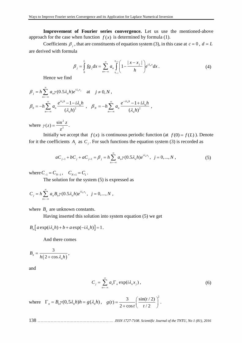
Ways to Improve Fourier series Convergence and its Application for Laplace Numerical Inversion
138 ……………………………………………………………. .ISSN 1727-7108. Scientific Journal of the TNTU, No 1 (81), 2016
Improvement of Fourier series convergence. Let us use the mentioned-above
approach for the case when function ( )f x is determined by formula (1).
Coefficients j
, that are constituents of equation system (3), in this case at 0c , d L
are derived with formula
1
10
| |1
i
n
i
xL
j i x
j j n
n x
x xfg dx a e dx
h
. (4)
Hence we find
(0.5 ) n ji x
j n n
n
h a h e
at 0,j N ,
0 2
1
( )
ni h
n
n
n n
e i hh a
h
, 2
1
( )
ni h
n
N n
n n
e i hh a
h
,
where 2
2
sin( )
zz
z .
Initially we accept that ( )f x is continuous periodic function (at (0) ( )f f L ). Denote
for it the coefficients j
A as j
C . For such functions the equation system (3) is recorded as
1 1(0.5 ) , 0,...,n ji x
j j j j n n
n
aC bC aC h a h e j N
, (5)
where 1 1NC C
, 1 1N
C C .
The solution for the system (5) is expressed as
(0.5 ) , 0,...,n ji x
j n n n
n
C h a B h e j N
,
where nB are unknown constants.
Having inserted this solution into system equation (5) we get
exp( ) exp( ) 1n n n
B a i h b a i h .
And there comes
3
2 cosn
n
Bh h
,
аnd
exp( )j n n n j
n
C a i x
, (6)
where (0,5 ) ( )n n n n
B h h g h ,
23 sin( / 2)
( )2 cos / 2
tg t
t t
.

Тetyana Solyar
ISSN 1727-7108. Вісник ТНТУ, № 1 (81), 2016 …………………………………………………………………………………. 139
To find solution for equation system (3) in general case (when (0) ( )f f L ) one has to
additionally investigate relevant to it homogenous system which is recorded as
* * *
1 10
j j jaA bA aA
, 0,...,j N .
The general solution for this difference equation system is
*
1 1 2 2
j j
jA U U ,
where 1,2
U are arbitrary constants, 1,2 are roots of equation
2
0a b a ,
that are equal to 1,22 3 .
Then the full solution for the equation system (3) is recorded as
2
1 1 2
2
j j
j j N
UA C U
.
The first system equation (3) is solved identically. Out of two last equations we obtain
the following system
1 1 2 2 2 0 0 1
1
1 1 1 2 2 1
0,5 0,5 0,5 ,
0,5 0,5 / 0,5 .
N
N
N N N
U b a U b a bC aC
U b a U b a bC aC
At 10N practically precise solution to this system can be recorded in simple manner
0 0 1 0 0 1
1
1
0,5 6 / 2,
0,5 3
bC aC h C CU
b a
1 1
2
2
0,5 6 / 2
0,5 / 3
N N N N N NbC aC h C C
Ub a
.
Thus, we have
1 1 2 2( ) exp( )
j j N
j n n n j
n
f x a i x U U
. (7)
For periodic functions the joint points can be selected at random and we will get the
formula for series calculation
( ) exp( )n n n
n
f x a i x
.
At large arguments values 2
( ) ( )g t O t
, i.e. 2( ) 0
nO n
as n , so the
series (7) converges faster than initial series (4). The coefficients n are defined by means of
function g. The graph of this function is displayed on Figure 1.

Ways to Improve Fourier series Convergence and its Application for Laplace Numerical Inversion
140 ……………………………………………………………. .ISSN 1727-7108. Scientific Journal of the TNTU, No 1 (81), 2016
Figure 1. The graph of function g
Figure 1 shows that in order to improve the convergence of slow-converging series it is
worth to limit terms in M series. They have to be selected in such way that 2 ,4M
h , i.e.
accept M N or 2M N . Here the first series terms will be least due to the close to zero
values of n multipliers.
The next one is the example highlighting the peculiarities of the formula (6). We accept
that ( ) sign( ),f x x x , i.e. the function is split. Fourier series distribution for this
function is
1
4 sin(2 1)( )
2 1n
n xf x
n
. (8)
Having used the formulas to improve the convergence we get (function f is periodic)
1
4 sin(2 1)( )
2 1n
n
n xf x
n
. (9)
At 2 /h N in nodal points j
x hj the precise value of this function is
( ) sign( )(1 )j
j jf x x , where 2 3 . (10)
Here N is an arbitrary integer number, 0, 1, 2,...j .
Out of formula (10) it is seen that relative error of the formula (9) in nodal points is
equal to j
j . This error is alternating and decreases fast during counter-wise movement
from point of discontinuity because -0.2679 . Maximal error value is reached in the first
point. In the third point the relative error is less than 2 per cent.
Table 1 displays the function f(x) in nodal points at 60N and at series (8) there are
10000 terms (2nd column) and 60 terms ( ( )N
f x , 3rd column). The 4th and 5th columns display the
precise f function value and approximate series value (9) when they retain 60 terms ( ( )N
f x ).

Тetyana Solyar
ISSN 1727-7108. Вісник ТНТУ, № 1 (81), 2016 …………………………………………………………………………………. 141
Table № 1
Estimation of efficiency of the formula of convergence improvement (9) for the series (8)
x ( )f x ( )N
f x ( )f x ( )N
f x
0 -0,00009 0 0 0
0,1047 1,0003 0,90264 1,26302 1,26795
0,2094 1,00016 0,94957 0,93026 0,9282
0,3142 0,9998 0,96585 1,01893 1,01924
0,4189 1,00008 0,97399 0,99503 0,99484
0,5236 1,00006 0,97882 1,00139 1,00138
0,6283 0,99991 0,98197 0,99966 0,99963
0,7330 1,00005 0,98416 1,00011 1,0001
0,9425 0,99992 0,98689 1,00001 1,00001
1,0472 1,0001 0,98775 1 1
1,2566 0,99996 0,98885 1 1
1,3614 1,00003 0,98916 1 1
1,5708 0,99994 0,98939 1 1
Table 1 displays that to sum up directly the slowly converging series with high accuracy one has to calculate up to 10000 terms. The formula of convergence improvement allows finding of series value with accuracy higher than 1 per cent everywhere except for three nodal points being closest to point of discontinuity; the series in formula (6) is fast converging (data of 4th and 5th columns). The presented results illustrate inherent features of the selected formula of convergence improvement: high accuracy in the areas where the function is smooth; fast decreasing of errors during counter-wise movement from the function special points.
Let us use the obtained formula for convergence improvement of series that describe functions being used during conformable displaying of the exterior of the unit disk in given area
0
( ) , 1n
n
n
c c
,
where j
c are given coefficients.
The closest convergence of this series appears on the line where
, , . (11)
After convergence improvement in correlation (11) we get
. (12)
Having extended analytically this series we obtain approximate formula for conformable displaying
. (13)
Let us present some properties of formula (13). During application of this formula the ellipsis stays the ellipsis with the same correlation of semi-axis, but its dimensions grow into ( )g h times. Really, in general case for arbitrary allocation of ellipsis hole we get
( ) /a b c ,
where a, b, c are known constants.
int
0
( )n
n
c c e
ite 0 2t
int
0
( )n n
n
c c e
0
( ) /n
n n
n
c c

Ways to Improve Fourier series Convergence and its Application for Laplace Numerical Inversion
142 ……………………………………………………………. .ISSN 1727-7108. Scientific Journal of the TNTU, No 1 (81), 2016
Having applied the suggested convergence improvement we obtain
1( ) /a b c .
As result it is seen that at ~ 0.1h we have 1~ 1.001 , i.e. the dimensions remain
practically unchangeable. It also means that selected transformation retains rectilinear crack the same crack. The boundaries fragments being ellipses, straight lines, and cracks retain their forms except for small junction areas between them.
Fourier series convergence improvement in Laplace inversion formula on Prudnikov main formulas.
Let us study the problem of function f(t) allocation on the basis of popular Laplace
integral image 0
exp( )F s f t st dt
. We mark via constant the fact that function F s
is analytical at Re .s Then there exists the precise formula of original exterior through its
image [6]
, (14)
where ( 2 ) /n
s c ni l ; c is the constant to improve solution convergence ( Re( ) 0c ); l is a
certain constant, 0 t l
. (15)
As a rule, the series in formula (14) converges slowly due to the fact that for wide class
of functions ( ) 1 /n
F s O n , where at large n values the series is alternating. That is why
during series calculations with formula (14) one has to keep a large number of terms in it. Accordingly, it is problematic to use the formula (14) directly. In certain list of issues [7 – 9] for the class of functions with known values of the original and its derivative at 0t and at large values of the independent variable the were obtained the specified inversion formulas that facilitate calculating the original with controlled accuracy via fast converging series.
Let us investigate the wide-spread case when the only known fact is original, which can be approximated with predetermined accuracy by the first degree piecewise-continuous polynomials.
To apply formula (14) it is necessary to sum-up slowly converging series with predetermined accuracy
( ) exp(2 / ), 0n
n
S t A nit l t l
, where n nA F s .
We indicate that formula (7) can be efficiently applied with this purpose. As an example
let us study the image predetermined with the formula2 2
( ) 1F s s a , where consta . It
should be mentioned, that an original for this image is the function 0( ) ( )f t J at , where 0
( )J at
is the Bessel first class function. We accepted 8c , 1a , 6l and denied remainder term
1R , as it has small multiplier here 8 4
3 10e .
Table 2 displays values of precise function ( )T
y f t and relative error in per cent
1
1100T
T
y y
y
, 2
2100T
T
y y
y
,
1
1exp( / ) exp(2 / )
n
n
f t ct l F s nit l Rl
1
1
expn
R nc f t nl

Тetyana Solyar
ISSN 1727-7108. Вісник ТНТУ, № 1 (81), 2016 …………………………………………………………………………………. 143
where 1y is the function obtained on the basis of formula (7) at 60N (there are 60 terms in
series), 2y is starting series with 1000 terms.
Table № 2.
Precise values of the originals and the error of Laplace inversion formula
0( )y J x x
y e
T Ty 1
2 T
y 1 2
0,000 1,000 -1,014 -50,0 1,000 -1,345 -50,0 0,500 0,938 -0,153 0,099 0,607 -0,448 0,140 1,000 0,765 -0,226 0,013 0,368 -0,450 0,000 1,500 0,512 -0,349 -0,212 0,223 -0,450 -0,526 2,000 0,224 -0,717 1,206 0,135 -0,450 1,953 2,500 -0,048 2,523 6,725 0,082 -0,449 -3,985 3,000 -0,260 0,272 0,007 0,050 -0,453 0,039 3,500 -0,380 0,044 -3,236 0,030 -0,490 40,91 4,000 -0,397 -0,070 9,601 0,018 -0,769 -207,7 4,500 -0,321 -0,122 -20,03 0,011 -3,078 579,2 5,000 -0,178 0,623 0,333 0,007 -29,2 -11,47
As it can be seen from Table 2 the suggested formula (7) facilitates higher accuracy at
60 terms in series than direct calculation of series with 1000 terms. The most relative errors of
the formula (7) occur in points where function f(x) is small in terms of value.
Table 2 also displays the results of calculations for the function ( )t
f t e
, which image
is ( ) 1/ ( 1)F s s . We can see that original allocation accuracy due to formula (7) for this
function is also high.
Conclusions. The author suggested Fourier series convergence improvement for the
functions that can be approximated with sufficiently high accuracy with the method of least
squares by piecewise – continuous polynomials of the first degree along the entire task section
within a series. The obtained formulas are applied to improve the series convergences which
appear at Laplace numerical transformation by means of Prudnikov formula. The basic problem
in this method is reduced to finding the sum of slowly convergent Fourier series. Given
examples illustrate the efficiency of given approach for numerical determination the originals
on basis of their Laplace images.
References
1. Kalitkin N.N. Chislennye metody. Moscow, Nauka, 1978. 512 p. [In Russian]
2. Tikhonov A.N., Arsenin V.Ya. Metody resheniya nekorrektnykh zadach. Moscow, Nauka, 1974. 286 p.
[In Russian]
3. Kushnir R.M., Solyar T.Ya. Termopruzhnyi stan bahatozv"yaznykh plastynok za yikh nahrivu. Fizyko-
khimichna mekhanika materialiv, 2006, vol. 42, no. 6, pp 27 – 33 [in Ukrainian]
4. Kushnir R.M., Solyar T.Ya. Neustaleni temperaturni napruzhennia bilia kryvoliniynoho otvoru v plastyntsi
z teploviddacheiu pry nahrivi potokom tepla. Matematychni metody ta fizyko-mekhanichni polya, 2008, vol. 51,
no. 1, pp. 105 – 111 [in Ukrainian]
5. Maksymovych O.V., Solyar T.Ya. Vyznachennya tryvymirnykh temperaturnykh poliv u bahatozv"yaznykh
ortotropnykh tilakh za nahrivu dzherelamy ta potokamy tepla. Matematychni metody ta fizyko-mekhanichni polya,
2009, vol. 52, no. 1, pp. 188 – 192 [in Ukrainian]
6. Ditkin V.A., Prudnikov A.P. Operatsyonnoe vyschyslenie. Moscow, Vysshaya shkola, 1975. 407 p. [In
Russian]
7. Kushnir R.M., Maksymovych V.N., Solyar T.Ya. Vyznachennya nestatsionarnykh temperatur na osnovi
utochnenykh formul obernennya peretvorennya Laplasa. Fizyko-khimichna mekhanika materialiv, 2002, vol. 38,
no. 2, pp. 18 – 26 [in Ukrainian]
8. Maksymovych V.N., Solyar T.Ya. Utochnennye formuly dlya opredeleniya obratnoho preobrazovaniya
Laplasa i ikh prymenenie v zadachakh teploprovodnosti. Inzhenerno-fizicheskii zhurnal, 2002, vol. 75, no. 3,

Ways to Improve Fourier series Convergence and its Application for Laplace Numerical Inversion
144 ……………………………………………………………. .ISSN 1727-7108. Scientific Journal of the TNTU, No 1 (81), 2016
pp. 102 – 103 [in Belarusian]
9. Solyar T.Ya. Vyznachennia nestatsionarnykh temperaturnykh poliv u bahatozv"yaznykh plastynkakh z
teploviddacheiu. Prykladni problemy mekhaniky i matematyky, 2006, vol. 4, pp. 109 – 116 [in Ukrainian]
Список використаної літератури
1. Калиткин, Н.Н. Численные методы [Текст] / Н.Н. Калиткин. – М.: Наука, 1978. – 512 с.
2. Тихонов, А.Н. Методы решения некорректных задач [Текст] / А.Н. Тихонов, В.Я. Арсенин – М.:
Наука, 1974. – 286 с.
3. Кушнір, Р.М. Термопружний стан багатозв’язних пластинок за їх нагріву [Текст] / Р.М Кушнір,
Т.Я. Соляр // Фіз.-хім. механіка матеріалів. – 2006. – 42, №6. – С. 27 – 33.
4. Кушнір, Р.М. Неусталені температурні напруження біля криволінійного отвору в пластинці з
тепловіддачею при нагріві потоком тепла [Текст] / Р.М. Кушнір, Т.Я. Соляр // Мат. методи та фіз.-мех.
поля. – 2008. – 51, № 1. – С. 105 – 111.
5. Максимович, О.В. Визначення тривимірних температурних полів у багатозв’язних ортотропних
тілах за нагріву джерелами та потоками тепла [Текст] / О.В. Максимович, Т.Я. Соляр // Мат. методи та
фіз.-мех. поля. – 2009. – 52, № 1. – С. 188 – 192.
6. Диткин, В.А. Операционное исчисление [Текст] / В.А. Диткин, А.П. Прудников. – М.: Высшая
школа, 1975. – 407 с.
7. Кушнір, Р.М. Визначення нестаціонарних температур на основі уточнених формул обернення
перетворення Лапласа [Текст] / Р.М. Кушнір, В.М. Максимович, Т.Я. Соляр // Фіз.-хім. механіка
матеріалів. – 2002. – 38, № 2. – С. 18 – 26.
8. Максимович, В.Н. Уточненные формулы для определения обратного преобразования Лапласа и их
применение в задачах теплопроводности [Текст] / В.Н. Максимович, Т.Я. Соляр // Инж. физ. журн. –
2002. – 75, № 3. – С. 102 – 103.
9. Соляр, Т.Я. Визначення нестаціонарних температурних полів у багатозв'язних пластинках з
тепловіддачею [Текст] / Т.Я. Соляр // Прикл. проблеми механіки і математики. – 2006. – Вип. 4. – С. 109 –
116.
УДК 539.3
СПОСІБ ПОКРАЩЕННЯ ЗБІЖНОСТІ РЯДІВ ФУР’Є ТА ЙОГО
ЗАСТОСУВАННЯ ДЛЯ ЧИСЛОВОГО ОБЕРНЕННЯ
ПЕРЕТВОРЕННЯ ЛАПЛАСА
Тетяна Соляр
Інститут прикладних проблем механіки і математики
ім. Я. С. Підстригача НАН України, Львів, Україна
Резюме. Розв’язок широкого кола задач математичної фізики може бути отримано у вигляді
рядів Фур’є. При розгляді задач, що пов’язані з дослідженням локалізованих дій, отримують швидкозмінні
розв’язки, у зв’язку з чим ряди повільно збігаються. Для розв’язування складних задач метод рядів Фур’є
використовують сумісно з іншими підходами. Зокрема, при додатковому застосуванні методу граничних
елементів коефіцієнти рядів знаходяться шляхом розв’язування одно- або двовимірних інтегральних
рівнянь, що відповідно вимагає значного обсягу обчислень. При цьому коефіцієнти рядів знаходять з
певними похибками, що відповідно може призвести до втрати точності розрахунків. У таких випадках
актуальною є проблема покращення збіжності рядів з контрольованою точністю розрахунків. Нижче
запропоновано метод покращення збіжності рядів Фур’є для функцій, які можуть бути з достатньо
високою точністю апроксимовані методом найменших квадратів кусково-неперервними поліномами
першого степеня на всьому проміжку задавання ряду.
Ключові слова: ряди Фур’є, покращення збіжності рядів, кусково-неперервні поліноми,
конформне відображення, числове обернення перетворення Лапласа.
Отримано 03.03.16

ISSN 1727-7108. Вісник ТНТУ, № 1 (81), 201 …………………………………………………………………………….………..145
IN COMMEMORATION OF DR. OLEH M. SHABLIY.
On the 31st January 2016 the first
Rector of the Ternopil Ivan Pul’uj National
Technical University Dr. Oleh Shabliy,
aged 81, passed away.
He was a talanted scientist and a public
figure, highly intellectual person, tolerant
friend and colleague, Doctor of Sciences
(Physics and Mathematics), Professor,
Member of the Academy of Engineering
Sciences of Ukraine, Honoured Scientist of
Ukraine.
Dr. Oleh M. Shabliy was born on the
18th June 1935 in the Ternopil region. In
1958 he graduated from the Lviv Ivan
Franko State University. In 1963 he
defended the Candidate of Sciences thesis
and in 10 years he gained his Doctor of
Sciences Degree in Physics and
Mathematics.
In 1961 Dr. O. Shabliy started his
career as the Assistant of the Department of
the theoretical mechanics at the Ternopil
branch of the Lviv Politechnical Institute,
1963 – 1964 – Sin. Teacher, from 1964 till
1985 – Head of Department.
He challenged himself as the capable guide
and administrative manager: Director of the
Ternopil branch of the Lviv Politechnic
Institute (TBLPI, 1985 – 1991), Rector of
the Ternopil Instrument – making Institute
(1991 – 1997), Rector of the Ternopil Ivan
Pul’uj State Technical University (1997 –
2007). Besides, he has been one of the first
Doctors of Sciences (Physics and
Mathematics) in the Ternopil region (since
1974), Professor (since 1976), Member of
the Academy of Engineering Sciences of
Ukraine (since 1991), Honoured Scientist of
Ukraine (since 1992).
Being supervised by him the Ternopil
branch of the Lviv Politechnics developed
and maintained facilities, trained teaching
staff, which resulted in reorganisation of the
institution into the Ternopil Instrument –
making Institute in 1991. Inspired by
Academician O. Shabliy, the Institute was
named after Ivan Pul’uj, famous Ukrainian
physicist, electrical engineer, public figure
and the patriot of Ukraine.
In two years the Ternopil Ivan Pulu’j
State Technical University was founded, the
4th accreditation level institution, on the
basis of the Instrument – making Institute,
where he was elected as the first Rector.
Having become more academically
ambitious our University gained the
membership in the European Association of
Universities in 1999, and in 6 years it joined
the Magna Gharta Universitatum.
During the period of 1991 – 2007 years
Dr. O. Shabliy strived to facilitate the
progress in educational and teaching
excellence, paying special attention to
physical training of students. We honour his
philosophy of education: TO TEACH, TO
EDUCATE, TO CULTIVATE HEALTHY
LIFE STYLE as the pre-conditions to equip
students with a high level of knowledge and
to adjust them to a new academic culture.
He seeked to provide comfortable rooms,
designed to accomodate the needs of
students and the staff. Estate facilities
comprise about 100 thousand squre meters,
accomodating more than 900 computer
users connected in local net and having
good WF access, 85 special teaching –
scientific laboratories, 33 computer classes,
scientific – technical library, provided with
audio-visual support and other AV services,

146 ……………………………………………………………. .ISSN 1727-7108. Scientific Journal of the TNTU, No 1 (81), 2016
educational-art and sport-training complex
«Politechnic», which includes concert – hall
accomodating 650 people, conference –
hall, canteen, versatile sport ground, gyms
and 25-meter long swimming pool.
During all his career the scientist
strived to facilitate and generate new
knowledge and understanding of the
potential for progress and to foster new
research agendas. In 1978 he founded a
scientific school «Facilitation of the stress-
strain state of solid fractured bodies», where
the problem of the solid fractured bodies
mechanics, optimal manufacturing process
design, heating systems design,
development and design of the satellite
television and communication antennae
have become of paramount importance. He fostered high – level cooperation
for many years between our University and the Institute for Electric Welding named after Y.O. Paton (IEW) of the National Academy of Sciences of Ukraine paying special attention to the welding production technologies. Investigations in the development of the energy – saving technologies of the induction fusion of the structure thin elements, recovering of the weared railway wheel pairs and mathematic modeling of the stress-strain state kinetics under multiple-pass welding of the structure elements, taking into account the phase transformation, have been carried out. Nurturing academic ambitions and being promoted by IEW the department «Technologies and equipment of the welding production» has been founded, where under the supervision of Dr. Oleh M. Shabliy the Candidate’s Degree Thesis and the Doctor’s Degree Thesis in the field of welding have been defended.
Aiming to build bridges between science and production the Rector of our University started the Technologies Transfer Center (TTC) by pioneering what has never been tried in more than ten areas in different fields of fundamental and applied sciences, Welding Technologies Center (WTTC) in particular, of the Ternopil Ivan Pul’uj National Technical
University. Development and application of
new energy-saving technologies for
strengthening and recovering of weared
machine parts and mechanisms for the
national economy have become
challenging.
Famous scientist has supervised and
was the Head of more than ten International
all-Ukrainian scientific symposia,
conferences and working-shops, the
International scientific – educational
Conference, I. Pul’uj’s Readings in
particular, dedicated to the 150th
anniversary of the famous physicist our
University is named after.
Dr. Oleh M. Shablij was the author of
more than 250 edited scientific papers,
2 monographies, the owner of 25 invention
patents of Ukraine, the owner of 20
Author’s rights Certificates. Some results of
scientific investigations are published in
foreign journals, in «Automatic Welding»
in particular.
A man of ideas and a man of action, he
was seeking to impart his knowledge to
young scientists promoting reasoning skills
and training. He supervised three Doctor’s
Degree theses and twelve Candidate’s
Degree theses in the field of engineering
and physical – mathematic sciences. Ten
scientific – investigation production –
related topics were researched under his
supervision. During this period the
University was ranked as one of the top
Universities of Ukraine.
His scientific activity was successfully
incorporated with the scientific –
management and public activity: he was the
Counsil Head of the Technologies Transfer
Center of the University (2006 – 2016),
Head of the Ternopil regional Fund named
after Ivan Pul’uj (1997 – 2016), Head of the
Ternopil Organisation of the Ukrainian
Union of the scientific – engineering
intellectuals (2002 – 2016), supervisior
of the Ternopil scientific – coordenation
Counsil of the Western scientific center of
the National Academy of Sciences of
Ukraine and the Ministry of Education of
Ukraine (1985 – 2000), supervisor of the

ISSN 1727-7108. Вісник ТНТУ, № 1 (81), 2016 …………………………………………………………………………………. 147
scientific working – shop on the solid body
mechanics and optimisation methods, Head
and a member of Academic Counsils for
defending Candidate’s and Doctor’s theses,
Head of the educational scientific –
production complex «Svitlo», Chief Editor
and a member of the Editorial Board of the
«Digest of the Ternopil National Technical
University» (1996 – 2007).
Academician Oleh M. Shabliy was
awarded by the Badge of Honour (1986),
Badge for Public Service (third class, 2009).
Gold medal of the American Biographic
Institute of the USA (2008). He was
decorated by the order «St. Sophia» (2005),
«Petro Mohyla» of the Ministry of
education of Ukraine (2007), Diploma of
the All-Union Programs «Ukraine National
Leaders» (2013) and «Fuel – energy
complex of Ukraine» (2013). Cambridge
International Bibliographic Center
recognised him as the Person of the year in
1998 in the nomination «Science».
Dr. Oleh M. Shabliy was Honourable
Citizen of Ternopil (since 2003).
Dr. Oleh M. Shabliy should be paid
tribute to for gaining the status of the
National University. Since 2007 he has
been working as the Vice – Rector
(Production Cooperation Affairs) and as the
Head of the department of programming
and mathematic modeling of the Ternopil
Ivan Pul’uj National Technical University.
Oleh Mykolayovych Shabliy is a
notable person in our society. He strived to
nurture academic ambitions to contribute
the people of Ukraine. He has been working
hard for all his life having benefited our
University, our town, our country.
Dr. Oleh Shabliy was open – hearted
person, wise and faithful. He was not only a
good leader and manager, devoted scientist,
but close friend, imparting colleague and
supervisor of young scientists. His
phylosophy of live and success was «To
live – is to work. This is what makes the life
of people notable».
University alumni appreciate his
contribution in challenging their scientific
careers and express their gratitude to a
Teacher. He inspired to aim high adjusting
young people to a new academic culture,
educating new generation of the scientific
engineering intellectuals.
In loving memory of Oleh
Mykolayovych Shabliy.
Ternopil Ivan Pul’uj National Technical
University
The E.O. Paton Electric Welding Institute
of the National Academy of Sciences of
Ukraine
Edition Board of «Avtomaticheskaya
svarka».

148 ……………………………………………………………….ISSN 1727-7108. Scientific Journal of the TNTU, No 1 (81), 2016
ПАМ’ЯТІ ОЛЕГА МИКОЛАЙОВИЧА ШАБЛІЯ
31 січня 2016 року на 81-му році
життя перестало битися серце першого
ректора Тернопільського національного
технічного університету імені Івана
Пулюя, талановитого вченого і
громадського діяча, людини високого
інтелекту, доброго товариша та колеги,
доктора фізико-математичних наук,
професора, дійсного члена Академії
інженерних наук України, заслуженого
діяча науки і техніки України Шаблія
Олега Миколайовича. Він народився
18 червня 1935 року на Тернопільщині.
1958 р. закінчив Львівський державний
університет імені Івана Франка. 1963 р.
захистив кандидатську дисертацію, а
через 10 років — докторську.
Олег Шаблій 1961 року розпочав
трудову діяльність із посади асистента
кафедри теоретичної механіки
Тернопільського загальнотехнічного
факультету Львівського політехнічного
інституту. Від 1963 до 1964 року був
старшим викладачем, а від 1964 до 1985
року – завідувачем цієї ж кафедри.
Олег Миколайович пройшов довгий
шлях адміністративно-організаційної
роботи як умілий і далекоглядний
керівник: директор Тернопільського
філіалу Львівського політехнічного
інституту (ТФЛПІ) (1985 – 1991 рр.),
ректор Тернопільського приладобудів-
ного інституту (1991 – 1997 рр.), ректор
Тернопільського державного технічного
університету імені Івана Пулюя (1997 –
2007 рр.). Окрім того, він став одним із
перших докторів фізико-математичних
наук на Тернопільщині (від 1974 р.),
професором (від 1976 р.), дійсним
членом Академії інженерних наук
України (від 1991 р.), заслуженим діячем
науки і техніки України (від 1992 р.).
У Тернопільській філії Львівської
політехніки за його керівництва було
інтенсивно розвинуто матеріально-
технічну базу і зміцнено кадровий склад.
Це дало змогу 1991 року реорганізувати
навчальний заклад у Тернопільський
приладобудівний інститут. За ініціативи
академіка О.М. Шаблія 1995 р. інституту
було присвоєно ім’я видатного
українського фізика, електротехніка,
громадського діяча і патріота Івана
Пулюя.
Через два роки на базі
приладобудівного інституту він
ініціював створення навчального
закладу IV рівня акредитації –
Тернопільський державний технічний
університет імені Івана Пулюя, де його
обрали першим ректором. Великим
досягненням стало те, що 1999 р. виш
набув членства в Європейській Асоціації
Університетів, а через 6 років
приєднався до Болонської Хартії
Університетів – Magna Gharta Universita-
tum.
За час ректорства Олега
Миколайовича (1991 – 2007 рр.) було
здійснено велику роботу з
удосконалення навчального процесу,
патріотичного виховання та фізичного
зміцнення молоді, що стало підґрунтям
для успішного впровадження триєдиної
моделі: НАВЧИТИ, ВИХОВАТИ,
ОЗДОРОВИТИ як необхідної умови
здобуття якісної освіти, гармонійного
розвитку та фізичного зміцнення
студентів. Керівник робив усе, для того
ISSN 1727-7108. Вісник ТНТУ, № 1 (81), 2016 …………………………………………………………………………………. 149
щоби забезпечити комфортні умови
студентам і працівникам. Насамперед
він створив матеріально-технічну базу:
близько 100 тис. м2 площі, понад
900 робочих комп’ютерних місць,
об’єднаних у локальну мережу з
виходом в Iнтернет, 85 спеціалізованих
навчально-наукових лабораторій, 33
комп’ютерні класи, науково-технічна
бібліотека з електронною читальною
залою, освітньо-мистецький і навчаль-
ний спортивно-оздоровчий комплекс
«Політехнік», до складу якого входять
простора актова зала на 650 місць,
конференц-зала, студентське кафе,
універсальна ігрова спортивна зала,
тренажерні зали та 25-метровий басейн.
Все це стало основою для втілення
високого рівня навчального і виховного
процесу.
Упродовж усієї трудової діяльності
вчений особливу увагу приділяв освіті та
підготовці наукових кадрів. Для цього
1978 року заснував наукову школу
«Оптимізація керування напружно-
деформованим станом деформівних
твердих тіл», де тема механіки
деформівного твердого тіла,
оптимального проектування технологіч-
них процесів, проектування нагріваль-
них систем, розробки і проектування
антен супутникового телебачення і
зв’язку стала предметом основних
досліджень.
За час багаторічної співпраці з
Інститутом електрозварювання (ІЕЗ)
імені Є.О. Патона НАН України
професор зосереджував велику увагу на
технологіях зварювального виробницт-
ва. Так, за його активної участі
проводилися дослідження з розробки
енергоощадних технологій індукційного
наплавлення тонких елементів
конструкцій, відновлення спрацьованих
залізничних колісних пар та
математичне моделювання кінетики
напружено-деформованого стану при
багатопрохідному зварюванні елементів
конструкцій з урахуванням фазових
перетворень. Завдяки його ж ініціативі
та підтримці ІЕЗ 1988 року було
створено кафедру «Технології і
обладнання зварювального виробницт-
ва», де безпосередньо під керівництвом
О.М. Шаблія працівники кафедри
захистили кандидатську і докторську
дисертації в галузі зварювання.
З метою забезпечення інтеграції
науки з виробництвом тодішній ректор
заснував Центр трансферу технологій
(ЦТТ), який на сьогодні має більше
десяти напрямів роботи у різних галузях
фундаментальної та прикладної науки,
зокрема Центр трансферу зварювальних
технологій (ЦТЗТ) Тернопільського
національного технічного університету
імені Івана Пулюя. Його основним
завданням стала розробка і
впровадження нових енергоощадних
технологій для зміцнення та відновлення
спрацьованих деталей машин і
механізмів для народного господарства.
Відомий вчений очолював роботу
більше десяти міжнародних,
всеукраїнських наукових симпозіумів,
конференцій та семінарів, серед яких
Міжнародна науково-освітня конферен-
ція з Пулюєвими читаннями, присвячена
150-річчю від дня народження відомого
фізика, ім’я якого носить ТНТУ.
Академік був автором понад 250-и
друкованих праць, зокрема 2-х
монографій, 25-ти патентів України на
винаходи, 20-и свідоцтв авторських прав
на новітні технології. Низку наукових
досліджень опубліковано в закордонних
виданнях і у журналі «Автоматическая
сварка».
Мудрий наставник щедро ділився
своїми знаннями з молоддю і сприяв
підвищенню фахового рівня наукових
кадрів. Він був керівником трьох
докторських і 12-и кандидатських
дисертацій у галузі технічних та фізико-
математичних наук. Десять науково-
дослідних тем за державним
замовленням, а також замовленням
юридичних осіб було виконано під його
150 ……………………………………………………………. .ISSN 1727-7108. Scientific Journal of the TNTU, No 1 (81), 2016
керівництвом. За час перебування
О.М. Шаблія на посаді ректора
університет мав один із найвищих
рейтингів серед ВНЗ України.
Плідну наукову роботу Олег
Миколайович успішно поєднував із
науково-організаційною і суспільною:
голова ради директорів Центру
трансферу технологій університету
(2006 – 2016 рр.), голова Тернопільсь-
кого обласного фонду імені Івана Пулюя
(1997 – 2016 рр.), голова Тернопільської
організації Українського союзу науково-
технічної інтелігенції (2002 – 2016 рр.),
керівник Тернопільської науково-
координаційної ради Західного науково-
го центру НАН України і МОН України
(1985 – 2000 рр.), керівник наукового
семінару з механіки твердого тіла і
методів оптимізації. Голова і член
спеціалізованих рад із захисту
кандидатських і докторських дисерта-
цій, голова навчально-науково-виробни-
чого комплексу «Світло», головний
редактор і член редколегії «Вісника
Тернопільського національного техніч-
ного університету» (1996 – 2007 рр.).
Академік О.М. Шаблій нагородже-ний
орденами «Знак пошани» (1986 р.) та «За
заслуги» ІІІ ступеня (2009 р.), золотою
медаллю Американського біографічного
інституту США (2008 р.). Відзначений
нагородою «Свята Софія» (2005 р.),
«Петро Могила» МОН України (2007 р.),
дипломами всеукраїнської програми
«Золотий фонд нації» (2013 р.),
всеукраїнської програми «Національні
лідери України» (2013 р.),
всеукраїнської програми «Паливно-
енергетичний комплекс України»
(2013 р.). Кембріджський міжнародний
бібліографічний центр 1998 р. визнав
його людиною року в номінації «Наука»,
а ще Олег Шаблій був почесним
громадянином міста Тернополя (2003 р.).
У наданні статусу університету
національного, безперечно, є його
велика заслуга: науковцю від 2007 року
вдалося здійснити чимало творчих
задумів на посадах проректора з питань
зв’язків із виробництвом та завідувача
кафедри інформатики і математичного
моделювання Тернопільського націо-
нального технічного університету імені
Івана Пулюя.
Олег Миколайович – це знакова
людина для суспільства. Він був тим
полум’ям, що запалювало пристрасне
прагнення служити науці, своєму
народові та Україні. Усе його життя – це
невтомна праця задля розвитку
університету, міста і країни.
Професор Шаблій – людина
глибокої віри, відкритості та мудрості.
Він був не лише хорошим керівником,
проникливим науковцем, а й добрим
другом, порадником для колег і
наставником для молоді. Не випадково
філософською квінтесенцією та
формулою його успіху стали слова:
«Жити – значить працювати. Праця є
життя людини».
Олег Миколайович Шаблій виховав
і проклав шлях у велику науку багатьом
учням, які безмежно вдячні за це своєму
Вчителеві. Він бачив у молодих людях
майбутнє країни, а тому всі свої сили і
розум віддавав вихованню нового
покоління науково-технічної інтеліген-
ції. Високо цінуючи дар життя, вчений
присвятив себе тому, щоби творити у
світі лише добрі та шляхетні справи.
Олег Шаблій житиме доти, доки його
будуть пам’ятати учні та будуть
продовжені його благородні починання.
Пам’ять про НЬОГО – чиста і
світла – назавжди залишиться в серцях
тих, хто знав, любив і поважав його.
Тернопільський національний
технічний університет ім. І. Пулюя
Інститут електрозварювання
ім. Є.О. Патона НАН України,
Редколегія журналу «Автоматическая
сварка»

ISSN 1727-7108. Вісник ТНТУ, № 1 (81), 2016 …………………………………………………………………………………. 151

152 ……………………………………………………………. .ISSN 1727-7108. Scientific Journal of the TNTU, No 1 (81), 2016
ВІСНИК ТЕРНОПІЛЬСЬКОГО
НАЦІОНАЛЬНОГО ТЕХНІЧНОГО
УНІВЕРСИТЕТУ
Науковий журнал
№ 1 (81) 2016
Редактори: А.В. Грицьків, Є.І. Гриценко
Коректор Н.Б. Коваль
Комп’ютерне макетування О.А. Дзядик
Тираж 125 пр. Зам. № 2659
Видавець Тернопільський національний
технічний університет ім. Івана Пулюя
вул. Руська, 56, м. Тернопіль, 46001
E-mail: [email protected]
Тел. 52-21-99, 42-79-65
Свідоцтво про внесення суб’єкта видавничої справи до державного реєстру видавців,
виготівників і розповсюджувачів видавничої продукції ДК № 4226 від 08.12.2011 р.