scientific computing

Scientific Computing

Linear Systems – LU Factorization

LU Factorization

• Today we will show that the Gaussian Elimination method can be used to factor (or decompose) a square, invertible, matrix A into two parts, A = LU, where: – L is a lower triangular matrix with 1’s on the

diagonal, and– U is an upper triangular matrix

LU Factorization

• A= LU

• We call this a LU Factorization of A.

LU Factorization Example

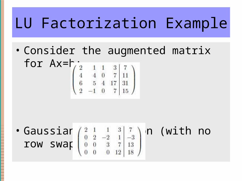
• Consider the augmented matrix for Ax=b:

• Gaussian Elimination (with no row swaps) yields:


• Let’s Consider the first step in the process – that of creating 0’s in first column:

• This can be achieved by multiplying the original matrix [A|b] by M1


• Thus, M1 [A|b] =

• In the next step of Gaussian Elimination, we pivot on a22 to get:

• We can view this as multiplying M1 [A|b] by


• Thus, M2 M1 [A|b] =

• In the last step of Gaussian Elimination, we pivot on a33 to get:

• We can view this as multiplying M2 M1 [A|b] by


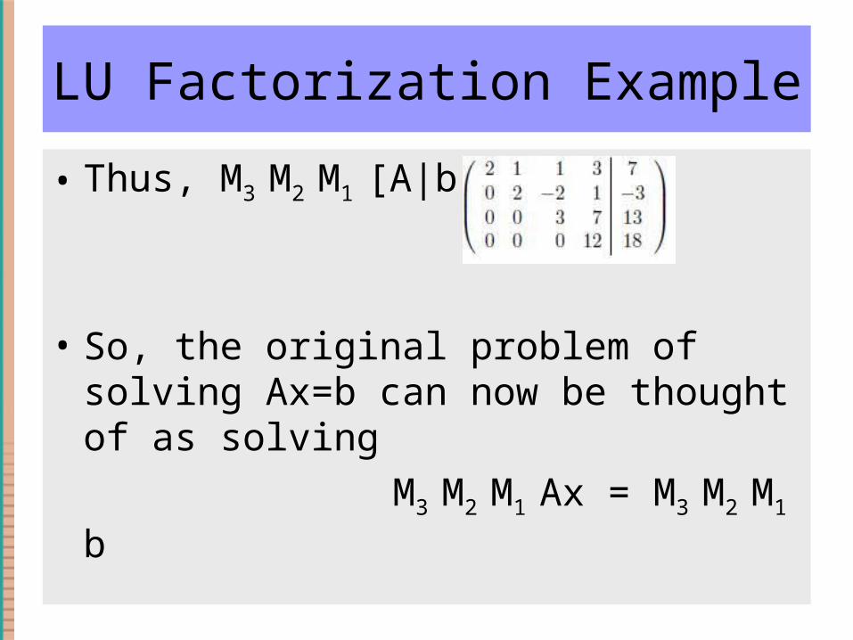
• Thus, M3 M2 M1 [A|b] =

• So, the original problem of solving Ax=b can now be thought of as solving

M3 M2 M1 Ax = M3 M2 M1 b


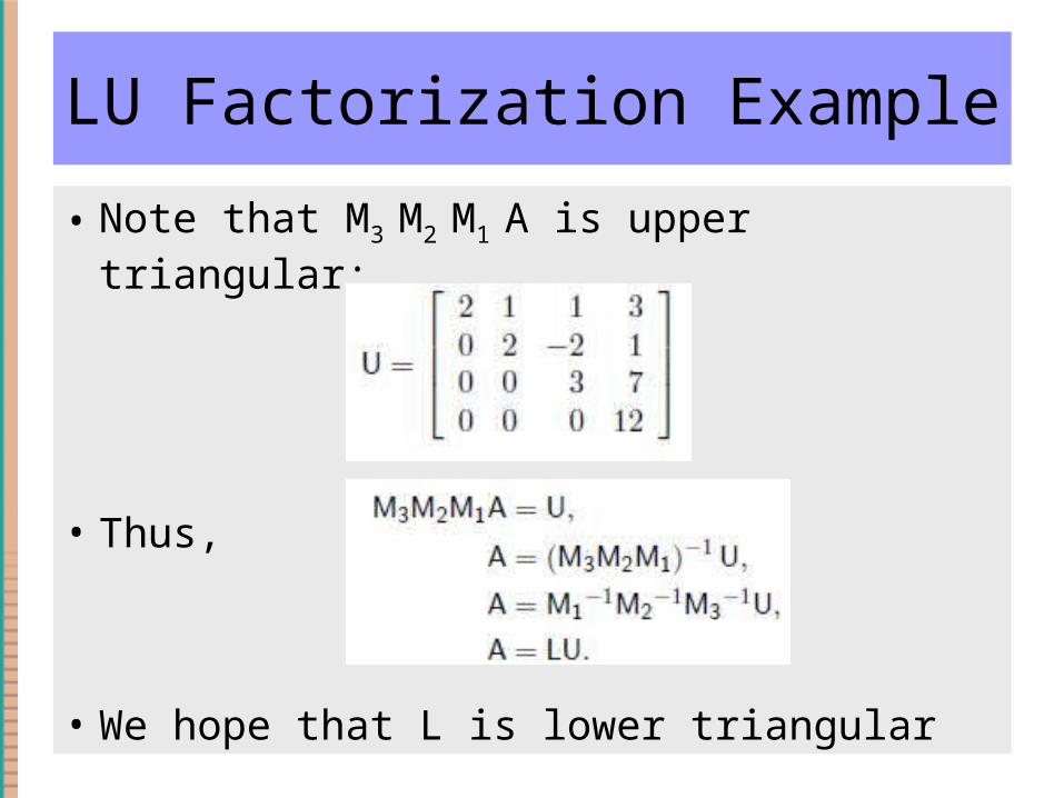
• Note that M3 M2 M1 A is upper triangular:

• Thus,

• We hope that L is lower triangular


• Recall: In Exercise 3.6 you proved that the inverse to the matrix

• Is the matrix


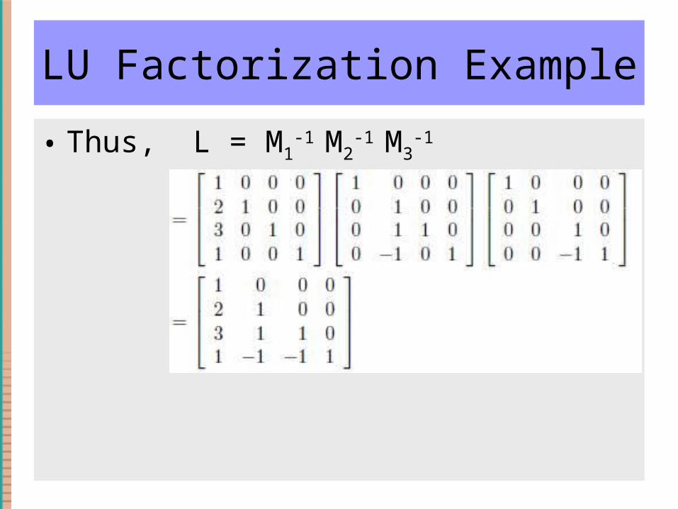
• Thus, L = M1-1

M2-1

M3-1


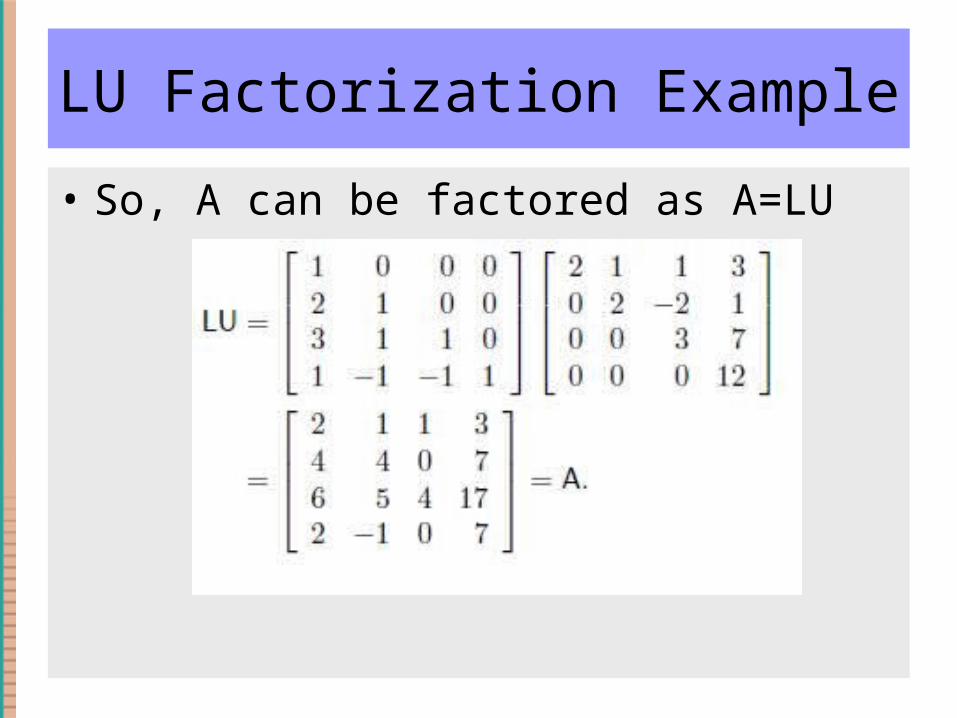
• So, A can be factored as A=LU

Solving Ax=b using LU Factorization

• To solve Ax=b we can do the following:– Factor A = LU– Solve the two equations:• Lz = b• Ux = z

– This is the same as L(Ux) = b or Ax=b.


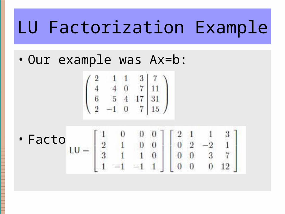
• Our example was Ax=b:

• Factor:


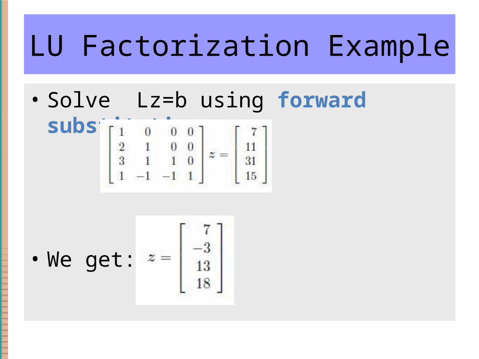
• Solve Lz=b using forward substitution:

• We get:


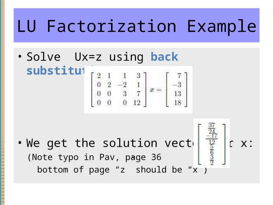
• Solve Ux=z using back substitution:

• We get the solution vector for x: (Note typo in Pav, page 36 bottom of page “z” should be “x”)

LU Factorization Theorem

• Theorem 3.3. If A is an nxn matrix, and Gaussian Elimination does not encounter a zero pivot (no row swaps), then the algorithm described in the example above generates a LU factorization of A, where L is a lower triangular matrix (with 1’s on the diagonal), and U is an upper triangular matrix.

• Proof: (omitted)

LU Factorization Matlab Function(1 of 2)

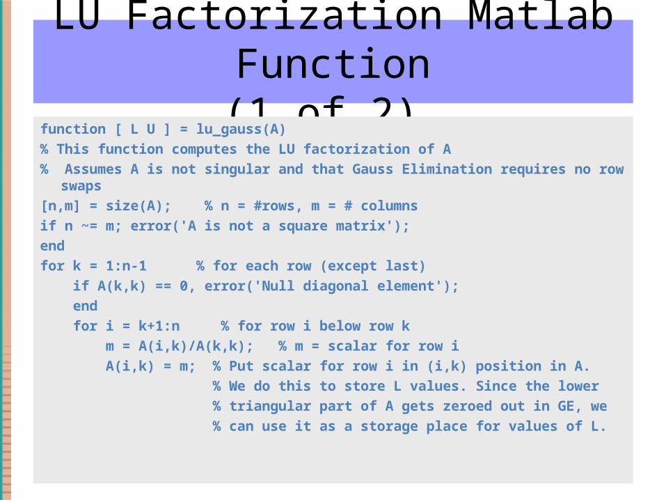
function [ L U ] = lu_gauss(A)% This function computes the LU factorization of A% Assumes A is not singular and that Gauss Elimination requires no row swaps[n,m] = size(A); % n = #rows, m = # columnsif n ~= m; error('A is not a square matrix');endfor k = 1:n-1 % for each row (except last) if A(k,k) == 0, error('Null diagonal element'); end for i = k+1:n % for row i below row k m = A(i,k)/A(k,k); % m = scalar for row i A(i,k) = m; % Put scalar for row i in (i,k) position in A. % We do this to store L values. Since the lower % triangular part of A gets zeroed out in GE, we % can use it as a storage place for values of L.

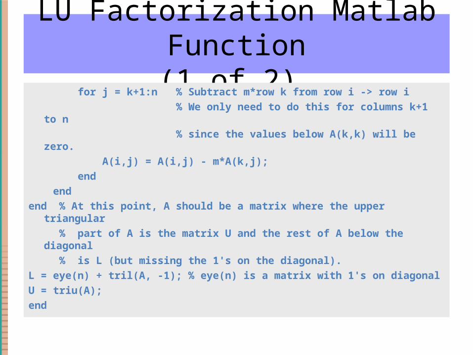
LU Factorization Matlab Function(1 of 2)

for j = k+1:n % Subtract m*row k from row i -> row i % We only need to do this for columns k+1 to n % since the values below A(k,k) will be zero. A(i,j) = A(i,j) - m*A(k,j); end endend % At this point, A should be a matrix where the upper triangular % part of A is the matrix U and the rest of A below the diagonal % is L (but missing the 1's on the diagonal). L = eye(n) + tril(A, -1); % eye(n) is a matrix with 1's on diagonalU = triu(A);end

LU Factorization Matlab

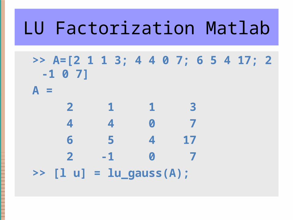
>> A=[2 1 1 3; 4 4 0 7; 6 5 4 17; 2 -1 0 7]A = 2 1 1 3 4 4 0 7 6 5 4 17 2 -1 0 7>> [l u] = lu_gauss(A);

LU Factorization Matlab

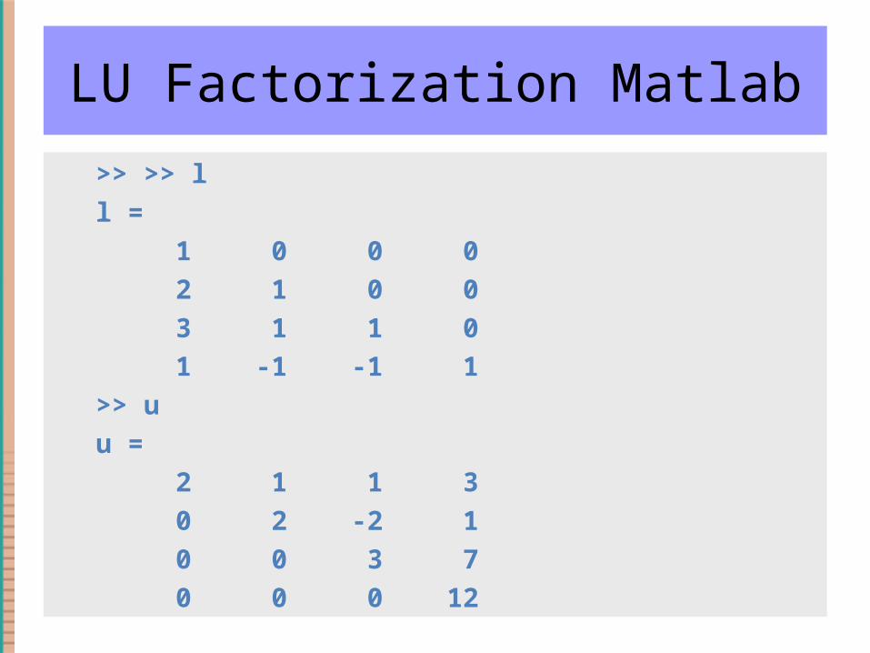
>> >> ll = 1 0 0 0 2 1 0 0 3 1 1 0 1 -1 -1 1>> uu = 2 1 1 3 0 2 -2 1 0 0 3 7 0 0 0 12

LU Factorization Matlab Solve Function

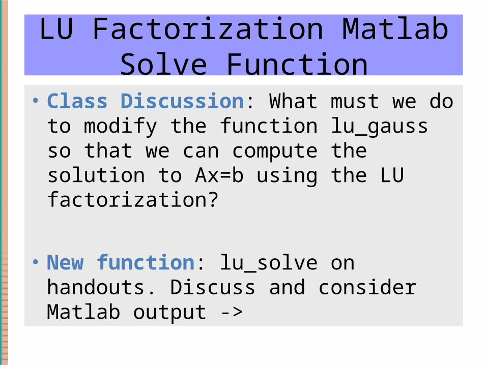
• Class Discussion: What must we do to modify the function lu_gauss so that we can compute the solution to Ax=b using the LU factorization?

• New function: lu_solve on handouts. Discuss and consider Matlab output ->

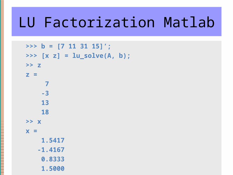
LU Factorization Matlab>>> b = [7 11 31 15]’;>>> [x z] = lu_solve(A, b);>> zz = 7 -3 13 18>> xx = 1.5417 -1.4167 0.8333 1.5000

Linear Algebra Review

• Now that we have covered some examples of solving linear systems, there are several important questions:– How many numerical operations does Gaussian

Elimination take? That is, how fast is it? – Why do we use LU factorization? In what cases

does it speed up calculation? – How close is our solution to the exact solution?– Are there faster solution methods?

Operation Count for Gaussian Elimination

• How many floating point operations (+-*/) are used by the Gaussian Elimination algorithm?

• Definition: Flop = floating point operation. We will consider a division to be equivalent to a multiplication, and a subtraction equivalent to an addition.

• Thus, 2/3 = 2*(1/3) will be considered a multiplication.

• 2-3 = 2 + (-3) will be considered an addition.


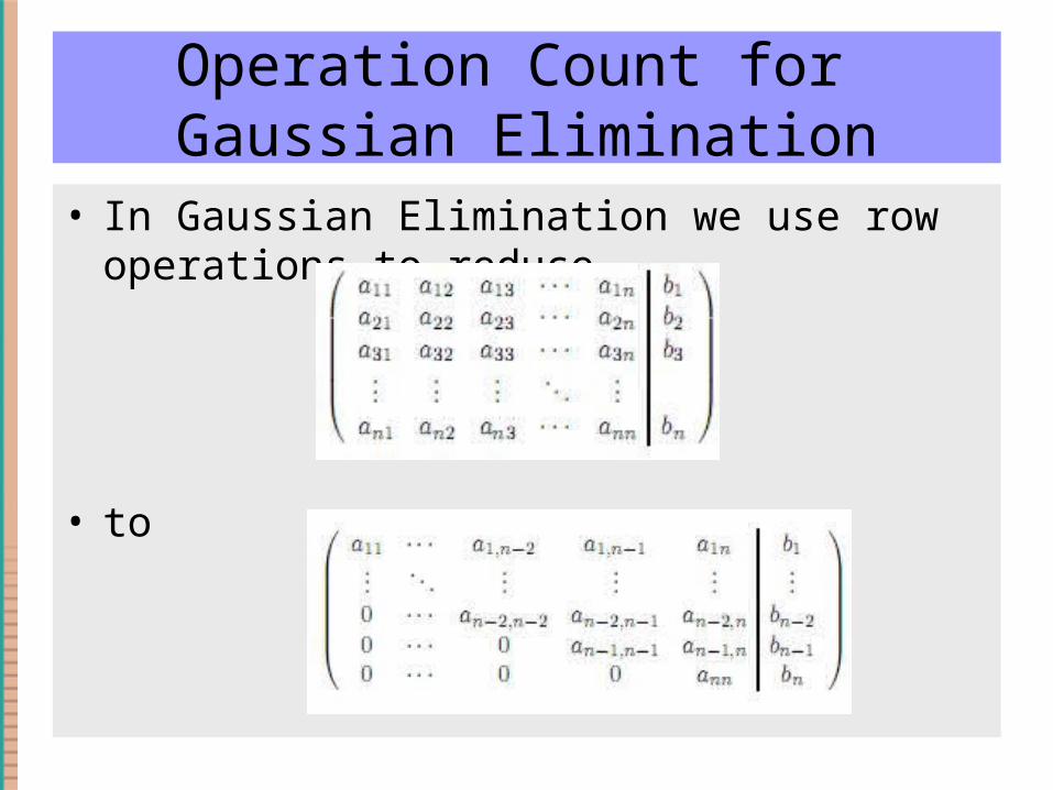
• In Gaussian Elimination we use row operations to reduce

• to


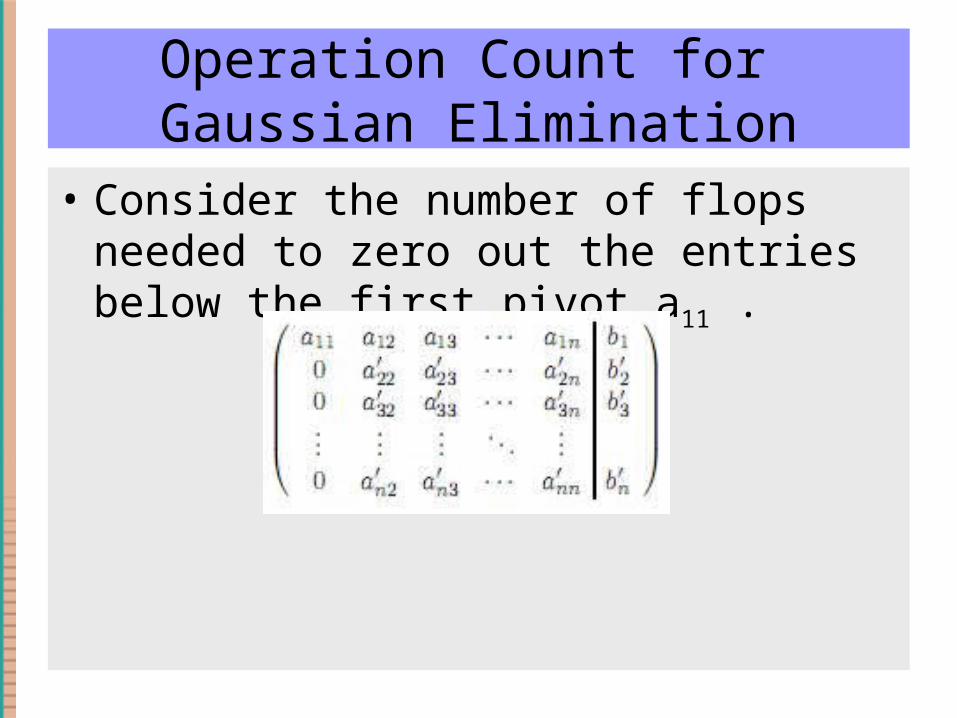
• Consider the number of flops needed to zero out the entries below the first pivot a11 .


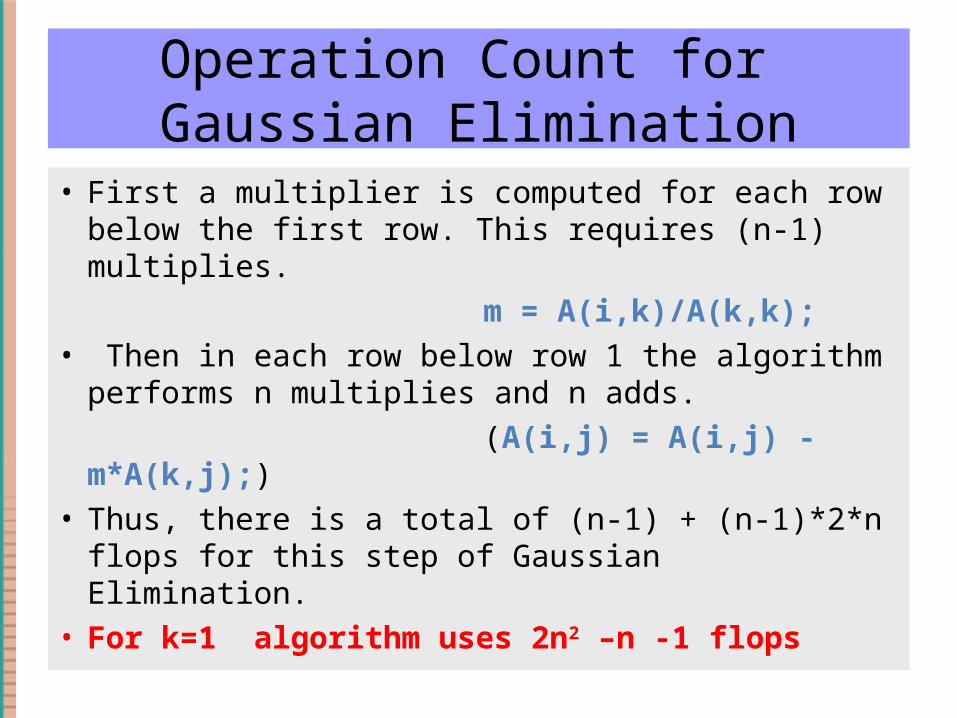
• First a multiplier is computed for each row below the first row. This requires (n-1) multiplies.

m = A(i,k)/A(k,k); • Then in each row below row 1 the algorithm

performs n multiplies and n adds. (A(i,j) = A(i,j) - m*A(k,j);) • Thus, there is a total of (n-1) + (n-1)*2*n flops for

this step of Gaussian Elimination. • For k=1 algorithm uses 2n2 –n -1 flops


• For k =2, we zero out the column below a22 .

• There are (n-2) rows below this pivot, so this takes 2(n-1)2 –(n-1) -1 flops.

• For k =3, we would have 2(n-2)2 –(n-2) -1 flops, and so on.

• To complete Gaussian Elimination, it will take In flops, where


• Now,

• So, In = (2/6)n(n+1)(2n+1) – (1/2)n(n+1) – n

= [(1/3)(2n+1)-(1/2)]*n(n+1) – n = [(2/3)n – (1/6)] * n(n+1) - n = (2/3)n3 + (lower power terms in n)• Thus, the number of flops for Gaussian

Elimination is O(n3).

Operation Count for LU Factorization

• In the algorithm for LU Factorization, we only do the calculations described above to compute L and U. This is because we save the multipliers (m) and store them to create L.

• So, the number of flops to create L and U is O(n3).

Operation Count for using LU to solve Ax = b

• Once we have factored A into LU, we do the following to solve Ax = b:

• Solve the two equations:• Lz = b• Ux = z

• How many flops are needed to do this?


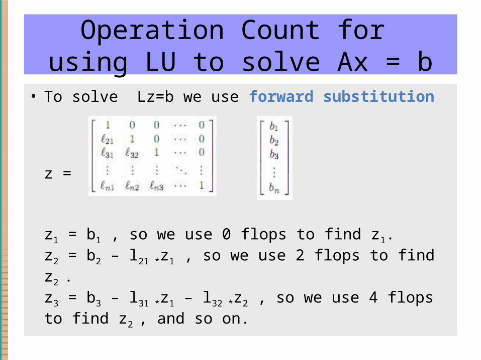
• To solve Lz=b we use forward substitution

z =

z1 = b1 , so we use 0 flops to find z1.z2 = b2 – l21 *z1 , so we use 2 flops to find z2 .z3 = b3 – l31 *z1 – l32 *z2 , so we use 4 flops to find z2 , and so on.


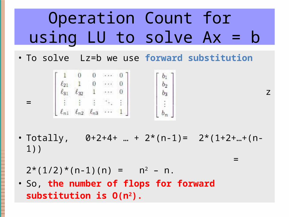
• To solve Lz=b we use forward substitution

z =

• Totally, 0+2+4+ … + 2*(n-1)= 2*(1+2+…+(n-1)) = 2*(1/2)*(n-1)(n) = n2 – n. • So, the number of flops for forward substitution is

O(n2).


• To solve Ux=z we use backward substitution

• A similar analysis to that of forward substitution shows that the number of flops for backward substitution is also O(n2).

• Thus, the number of flops for using LU to solve Ax=b is O(n2).

Summary of Two Methods

• Gaussian Elimination requires O(n3) flops to solve the linear system Ax = b.

• To factor A = LU requires O(n3) flops • Once we have factored A = LU, then, using L

and U to solve Ax = b requires O(n2) flops.

• Suppose we have to solve Ax = b for a given matrix A, but for many different b vectors. What is the most efficient way to do this?

Summary of Two Methods

• Suppose we have to solve Ax = b for a given matrix A, but for many different b vectors. What is the most efficient way to do this?

• Most efficient is to use LU decomposition and then solve

• Lz = b• Ux = z

• Computing LU is O(n3), but every time we solve Lz=b, Ux=z we use O(n2) flops!

scientific computing

Documents