science of sound laboratory manual - dissidents welcome to the first edition of science of sound...

Science of SoundScience of SoundLaboratory ManualLaboratory Manual

James M. FioreJames M. Fiore

2 Science of Sound Laboratory Manual

Science of SoundLaboratory Manual

by

James M. Fiore

Version 1.0.1, 07 March 2018


This Science of Sound Laboratory Manual, by James M. Fiore is copyrighted under the terms of a Creative Commons license:

This work is freely redistributable for non-commercial use, share-alike with attribution

Device datasheets and other product information are copyright by their respective owners

Published by James M. Fiore via dissidents

For more information or feedback, contact:James Fiore, ProfessorElectrical Engineering TechnologyMohawk Valley Community College1101 Sherman DriveUtica, NY 13501www.mvcc.edu/[email protected]

Cover photo Demarimbow by the author


http://www.dissidents.com/

mailto:[email protected]

http://www.mvcc.edu/jfiore

http://creativecommons.org/licenses/by-nc-sa/4.0/

PrefaceWelcome to the first edition of Science of Sound Laboratory Manual, an open educational resource (OER). The goal of this work is to support the lab portion of a general college physics course that focuses on sound, acoustics and audio. It covers a variety of topics including speed of sound, resonance, loudness, basic electricity (in association with loudspeakers and microphones) and the human voice. The following equipment should be available for each lab station: General purpose physics components including mass set, spring, stopwatch, meterstick/tape measure and an L-rod (hanger); electrical test gear including a digital oscilloscope, two sine wave generators, a voltmeter capable of reading dB, a DC power supply, two dynamic microphones such as the Shure SM-58 with mic pre-amps, PVC pipe, a pair of headphones and two raw frame loudspeakers (a 4” to 6” general purpose plus an 8” to 12” woofer). A purpose-built apparatus is required for the Tensioned String exercise along with different gauges of piano wire (long scale bass guitar strings can also be used) and a guitar pickup (a removable acoustic guitar pickup works well). A BNC switch box is handy for the Loudness exercise and is relatively easy to make. The Room Modes demo makes use of an SPL meter and a subwoofer or PA loudspeakerwith amplifier. Finally, a personal computer running Windows is required for the final four exercises. These exercises make use of the Sample Wrench free audio editor and analyzer. It is available from my web site www.dissidents.com.

I cannot say enough about the emerging Open Educational Resource movement and I encourage budding authors to consider this route. While there are (generally) no royalties to be found, having complete control over your own work (versus the “work for hire” classification of typical contracts) is not to be undervalued. Neither should contributions to the profession nor the opportunity to work with colleagues be dismissed. Given the practical aspects of the society in which we live, I am not suggesting that people “work for free”. Rather, because part of the mission of institutes of higher learning is to promote and disseminate formalized instruction and information, it is incumbent on those institutions to support their faculty in said quest, whether that be in theform of sabbaticals, release time, stipends or the like.

If you have any questions regarding this lab manual or my other OER works, or are interested in contributing to these projects, do not hesitate to contact me. Finally, please be aware that the most recent versions of all of my OER texts and manuals may be found at my MVCC web site as well as my mirror site: www.dissidents.com

AcknowledgmentsFor their continued support, my family and friends. For their input on draft versions, my colleagues and students. For continued sanity enhancement, musicians and composers to numerous to mention. For unintentional diversionary humor elicitation, Wally and pals (again).

Finally, a serious thank you, thank you, thank you to all of the people who have created useful software and other OER tools without which this project would have been impossible. When we each do a little, we all gain a lot. This text was created using free and open software applications including Open Office. Screen imagery was often manipulated though the use of XnView.

- Jim Fiore, 2016


http://www.xnview.com/en/

https://www.openoffice.org/



- Frank Zappa,Vibraphone ostinato from The Deathless Horsie


Table of Contents1. Force and Pressure . . . . . 8

2. Speed of Sound . . . . . 12

3. Simple Harmonic Motion . . . . 16

4. Tensioned String . . . . . 22

5. Resonant Pipes . . . . . 28

6. Human Voice: Range and Timbre . . . 32

7. Loudness . . . . . . 36

8. Basic Electricity . . . . . 42

9. Loudspeaker Impedance Magnitude . . 46

10. Microphone Patterns . . . . 50

11. Sample Wrench Audio Editor . . . 54

12. Equalization & Spectral Analysis . . . 64

13. Time Delay Effects . . . . . 66

14. Special Effects . . . . . 68

15. Room Modes Demonstration . . . 72


1 Force and PressureIntroductionIn this exercise, force and pressure are examined through direct observation in a qualitative manner. Force may be computed by multiplying the mass of an object by acceleration:

f=ma

If the mass is measured in kilograms and the acceleration in meters per second squared, the resulting unit of force is kilogram meters per second squared, or Newtons (N). For comparison, one pound of force is equivalent to approximately 4.45 N. A mass sitting on the Earth is affected by Earth’s gravitational acceleration, 9.8 m/s2, sothe force acting on it at rest (i.e., its weight) is the mass in kg times 9.8 m/s2.

Pressure is defined as force per unit area:

p=f/area

Given a force in Newtons and an area in square meters, the resulting unit (Newtons per square meter) is called a Pascal (Pa). Note that pressure can be increased by either increasing the force or by decreasing the area. Even a modest force can produce extremely high pressure if it is applied over an exceedingly small area.

Equipment1 meter stick or tape measure1 metric mass set1 metal plate1 sheet of foam rubber


Procedure

Part A: Calculating Force and Pressure

1. Calculate the expected force for the 1000 g (1 kilogram) mass based on the acceleration due to Earth’s gravity and record in Table 1.

2. Repeat step one for the 500 g and 200 g masses.

3. Measure the diameter of the 1000 g mass. Calculate the resulting area (area = π r 2) and record in table two. Using the force computed in Table 1, calculate and enter the resulting pressure in Table 2.

4. Repeat step three for the 500 g and 200 g masses.

Part B: Observing Pressure via Deformation

5. A simple qualitative way of observing pressure is to note the deformation of a semi-soft material. Inthis exercise, a slab of foam rubber will serve this purpose. Simply place the 1000 g mass on the slab and note the degree of deformation (none, slight, moderate, etc.). Enter your observation in the final column of Table 2

6. Repeat step five for the 500 g and 200 g masses.

7. Using the same force, pressure may be increased or decreased by decreasing or increasing the area, respectively. To increase the effective area, a metal plate may be introduced between the mass and foam rubber. Calculate the area of the plate, and based on this value, calculate the new pressures forthe three masses and enter these data in Table 3.

8. Place the metal plate on the foam rubber and position the 1000 g mass in its center. Note the degree of deformation of the foam rubber and record in Table 3.

9. Repeat step five for the 500 g and 200 g masses.

10. To illustrate the effect of decreasing the area, place the plate on the foam rubber on edge, that is, theplate should be perpendicular to the foam rubber. Carefully balance the 1000 g mass on the top edge of the plate (you will have to steady it with your hands) and note the deformation. The area in this instance is the area of the edge of the plate, and thus very, very small compared to the plate faceor the bottom of the mass. (This observation is sufficient and there is no need to attempt to measure the area of this edge.)


Data TablesMass Force

1000 g

500 g

200 g

Table 1

Mass Diameter Area Pressure Observations

1000 g

500 g

200 g

Table 2

Mass Plate Area Pressure Observations

1000 g

500 g

200 g

Table 3


Questions1. What is the affect of increasing mass on force?

2. What is the affect of increasing area on pressure?

3. Does the higher of two masses always produce a higher force given the same acceleration?

4. Does the higher of two masses always produce a higher pressure?

5. Based on established theory, if this exercise had been repeated on the moon, would you expect the deformations recorded in Tables 2 and 3 to be the same, greater, or smaller? Why?


2 Speed of SoundIntroductionThe speed of sound in air at room temperature is approximately 343 meters per second, or 1125 feet persecond, and increases with increasing temperature. This velocity is roughly equivalent to approximately1 foot every .9 milliseconds. Thus, for the dimensions of typical class and lab rooms, time delays are generally less than 50 milliseconds, and are therefore difficult to measure without specialized equipment. Digital oscilloscopes can easily resolve time differences several orders of magnitude less than one millisecond, and thus are a good candidate for this exercise. Care must be taken to make sure that no differential delay is caused by the recording circuitry.

Equipment

Digital Sampling Oscilloscope2 Microphones, stands, and cables (one cable at least 6 meters long)2 Microphone pre-amps (optional)Transient generator (clicker, wood blocks, etc.)

Procedure

1. Mount the microphones on the stands at a comfortable height, placing them relatively close to each other. Connect a short cable to the first microphone and a long cable to the second. Connect the microphones to the pre-amps (if available). Connect the pre-amp output for microphone one (short cable) to channel one of the oscilloscope, and similarly, connect the pre-amp output for microphonetwo (long cable) to channel two of the oscilloscope.

2. Depress the oscilloscope’s “Quick Menu” button and use the following settings: Input Coupling=AC, Input Impedance=1M, Bandwidth=20MHz. Set the Trigger Source to Channel One.

3. Adjust the oscilloscope time base (Horizontal Scale) to approximately 1 millisecond per division and the amplitude (Vertical Scale) to 5 mV per division if no pre-amps, and 100 mV otherwise. Position the Trigger Start Position toward the left edge of the display (this is the little orange triangle at the top of the grid; move it using the Horizontal Position knob).

4. Position the transient generator close to the microphones and equally distant from them. Generate a transient while observing the oscilloscope display. Adjust the vertical sensitivity scale so that the waveform peaks are seen clearly.


5. Using the sample capture/freeze ability of the oscilloscope (the “single shot” button on the extreme right side) adjust the Trigger Level control so that a transient triggers the oscilloscope. This will create a “freeze frame” of the transient events recorded by the microphones. This may take some trial and error. (Generate a transient and decrease the Trigger Level until the transient is captured. Ifthe level is set too low, false triggers will occur on random sounds.)

6. With the oscilloscope set properly, generate a transient and examine the waveforms on the oscilloscope.

7. Adjust the Vertical Position of the two waveforms so that the starting points are visible clearly. Record the time delay between channel one and channel two in Table 1. If the delay is considerably less than one millisecond, leave the velocity column blank. If not, make sure that the transient device is located equal distances from the microphones and try again.

8. Move the second microphone to a new position at least a few meters away from the first microphone.

9. Measure the distance between the two microphones and record in the first column of Table 1.

10. Set the Horizontal Scale to 2 milliseconds per division.

11. Generate a transient very close and somewhat to the side of the first microphone. Examine the waveforms on the oscilloscope. If the second channel transient is beyond the right edge of the display, increase the Horizontal Scale and try again. The Vertical Scale (or pre-amp gain) for the second microphone may need to be increased in order to see the transient waveform.

12. Measure the time delay between the two channels and record in Table 1. Based on this time and the separation recorded in column one, compute the velocity of sound and record in Table 1.

13. Repeat steps 8 through 12 for two other microphone separations. One of them should be at least 6 meters.


Data TablesSeparation Time Delay Velocity Comments

Equidistant

Table 1

Questions1. What is the purpose of initially setting the microphones next to each other?

2. Is the time delay constant, proportional, or inversely proportional to the separation distance?

3. Is the velocity of sound constant, proportional, or inversely proportional to the separation distance?

4. In general, if this experiment had been repeated outside on a very cold day, would the time delays have been longer, shorter, or the same for the distances used?


3 Simple Harmonic MotionIntroductionThe simple harmonic motion is examined in this exercise through the observation of a simple pendulum and a mass-loaded spring. A pendulum is an example of simple harmonic motion. For small displacements of the mass relative to the length of the pendulum, and assuming that the weight of the suspending rod or wire is negligible, the frequency of oscillation is

l

gf

21

where f is the frequency in Hertz, g is the gravitational attraction (9.8 m/s2 on Earth) and l is the length of the pendulum in meters. Note that longer pendulums produce a lower frequency of oscillation and that mass does not affect the frequency.

For the mass-loaded spring, the frequency of oscillation is

m

kf

21

where f is the frequency in Hertz, k is the spring constant in kilograms per second squared (higher values indicate a stiffer spring) and m is the suspended mass in kilograms. Note that a stiffer spring produces a higher frequency of oscillation and that a larger mass produces a lower frequency.

Equipment1 suspension arm1 meter stick1 length of string, approximately 1.5 meters1 metric hooked mass set1 lab-quality spring (k ≈10 N/m)1 stopwatch


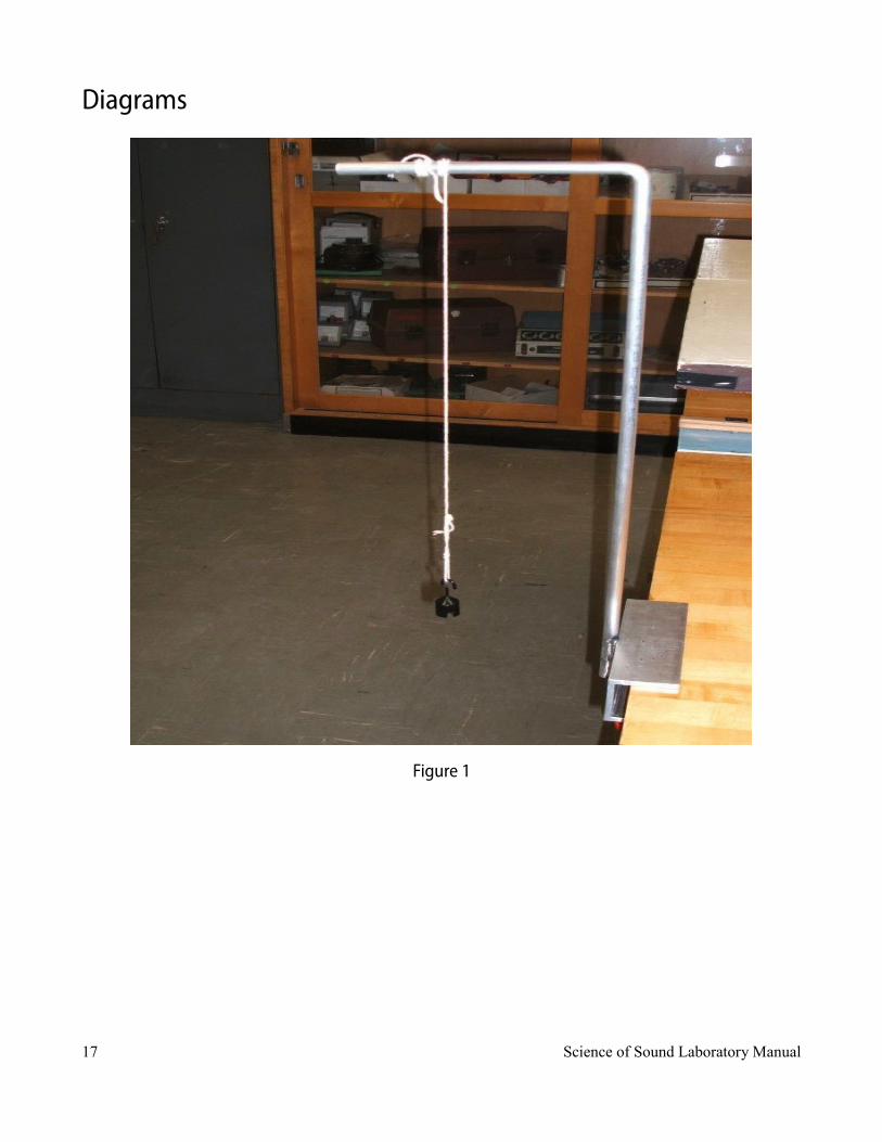
Diagrams

Figure 1


Figure 2

Procedure

Part A: Pendulum

1. Clamp the suspension arm to the side of the bench as shown in Figure 1. At one end of the string, tie a loop leaving over one meter of string dangling free. Hook on the 20 gram mass.


2. From the center of the mass, measure along the string to a point one meter away. Wrap the remaining string around the horizontal arm and suspend the mass away from any obstruction.

3. Move the mass horizontally from its resting position about one-tenth the length of the string. Let goof the mass and time how long it takes to complete 30 back-and-forth swings. Record this value in the first column of Table 1. Based on this value, compute the frequency of oscillation and record that value in the second column of Table 1. Also, record the theoretical value (predicted by formula)in the third column and place any comments or observations in the fourth column.

4. Repeat steps 2 and 3 above, first using a .5 meter length and then a .25 meter length, recording the appropriate values in Table 1.

5. Copy the values in the first row (1 meter) of Table 1 to the first row (20 grams) of Table 2.

6. Replace the 20 gram mass with a 50 gram mass.

7. Once again, measure along the string one meter away from the center of the mass. Pinch the string at this point and suspend the mass away from any obstruction.

8. Move the mass horizontally from its resting position about one-tenth the length of the string. Let goof the mass and time how long it takes to complete 30 back-and-forth swings. Record this value in the first column of Table 2. Based on this value, compute the frequency of oscillation and record that value in the second column of Table 2.

9. Repeat steps 7 and 8 above using a 100 gram mass in place of the 50, recording the appropriate values in Table 2.

Part B: Spring

10. Attach the spring to the arm so that it hangs vertically as shown in Figure 2 and attach a 200 gram mass to the bottom.

11. Deflect the mass downward and release. Caution: do not over stretch the spring so that the mass flies upward past the spring’s fully compressed position! Time how long it takes to complete 30 up-and-down cycles and record in column one of Table 3. Based on this value, compute the frequency of oscillation and record the value in the second and third columns of Table 3. Again, theory and observations go in the third and fourth columns.

12. Repeat step 11 using a 300 gram total mass and then a 500 gram mass.


Data Tables

Length Time Frequency (Exp) Frequency (Theory) Comments

1 meter

.5 meter

.25meter

Table 1

Mass Time Frequency (Exp) Frequency (Theory) Comments

20 grams

50grams

100grams

Table 2

Mass Time Frequency (Exp) Frequency (Theory) Comments

200grams

300grams

500grams

Table 3


Questions1. What is the affect of changing pendulum length on the frequency of motion?

2. What is the affect of changing mass on the pendulum’s frequency of motion?

3. What is the affect of changing mass on the spring’s frequency of motion?

4. Based on established theory, if this exercise had been repeated on the moon, would you expect the frequencies noted in Table 1 to be higher, lower, or the same?

5. What are the some of the possible sources of experimental error in this exercise and how might theybe reduced?


4 Tensioned String IntroductionA tensioned string is a classic example of controlled vibration which may create waveforms with many overtones or harmonics. This may result in a waveform considerably more complex in appearance than a simple sine wave although it will have a discernable period. Pythagoras studied the variables in the system circa 500 BCE and made important contributions to the science behind Western musical scales. The frequency of oscillation of a tensioned string is

u

T

lf

2

1

where f is the frequency in Hertz, T is the tension in kilogram meters per second squared (Newtons), u is the mass per unit length of the string in kilograms per meter, and l is the vibrating length of the stringin meters. In this experiment, the tension, T, is simply the product of a suspended mass (kilograms) times the acceleration due to gravity (9.8 meters per second squared). That is, tension is a force and force is equal to mass times acceleration. Note that longer strings and more massive strings produce a lower frequency of oscillation and that increased tension increases frequency.

Equipment

1 meter stick3 lengths of varying gauge steel piano wire, approximately 1.2 meters each, or guitar/bass strings1 metric hooked mass set1 tensioned string apparatus1 magnetic pickup1 oscilloscope1 microphone pre-amp


Diagram

Figure 1

Procedure

1. Connect the channel one output of the mic pre-amp to channel one of the oscilloscope with a BNC to BNC cable. Connect the magnetic pickup to the channel one input of the mic pre-amp with an alligator clip to BNC cable. Turn on the mic pre-amp and set the gain to 3/4ths maximum. Turn on the oscilloscope and select the Quick Menu button. For initial settings, set Bandwidth to 20 MHz instead of Full, set the Time Base to 10 milliseconds per division and the Amplitude to 50 millivolts per division.

2. Referring to Figure 1, connect one end of the first wire to the hook on the back of the apparatus. Feed the wire over the groove on top of the adjustable stop piece, over the pulley at the far end, andleaving the other end of the wire dangling free.

Variation of Mass

3. Adjust the movable stop of the apparatus (an Allen wrench may be required) so that the center of the stop is 1 meter away from the center of the pulley opposite.

4. Hook on the 1000 gram mass and position the pickup just below the center of the string (i.e., about .5 meters from the pulley or stop). There should only be about 5 mm (.2 inches) between the string and the pickup.

5. Pluck the string and watch the waveform on the oscilloscope. After the initial transient you should


see a fairly repeatable wave shape, although it may not appear perfectly sinusoidal. You can “freeze” the image by hitting the Capture/Single Shot button. Determine the time for one cycle based on the Time Base setting and the number of divisions in one cycle. The Vertical MeasurementCursors can make this job a little easier. Compute the frequency of oscillation and record that valuein the first column of Table 1. Alternately, if fairly clean waveforms can be produced consistently, the Frequency Measurement Function of the oscilloscope may be used. Also, compute the theoretical frequency value and place it in the second column. Place any comments or observations in the third column.

6. Repeat steps 4 and 5 above, first using 1500 grams and then 2000 grams, recording the appropriate values in Table 1.

7. Copy the values in the middle row (1500 grams) of Table 1 to the first row (1 meter) of Table 2.

Variation of Length

8. Apply 1500 grams total to the end of the wire.

9. Reposition the stop so that it is .5 meters from the center of the pulley and reposition the pickup so that it remains centered along the length of the wire. Pluck the string, determine and record the frequency as per step 5, recording the result in the second row of Table 2.

10. Reposition the stop so that it is .25 meters from the center of the pulley and reposition the pickup sothat it remains centered along the length of the wire. Pluck the string, determine and record the frequency as per step 5, recording the result in the third row of Table 2.

11. Copy the values in the middle row (.5 meters) of Table 2 to the first row (gauge one) of Table 3.

Variation of Wire Gauge (mass per unit length)

12. Return the stop to .5 meters and replace the wire with another gauge wire (or guitar/bass string as available). Configure it as indicated in step 2 and hook on 1500 grams. Position the pickup mid-wire again.

13. Pluck the string and determine the frequency, recording the result in the second row of Table 3.

14. Repeat steps 12 and 13 using the third wire gauge, recording the results in the third row of Table 3.

15. Using the final setup, move the pick up to various positions along the wire, plucking at each new location. Note how the wave shape changes at each position.


Data Tables

Mass Frequency (Exp) Frequency (Theory) Comments

1000grams

1500grams

2000grams

Table 1 (one meter length/wire gauge 1)

Length Frequency (Exp) Frequency (Theory) Comments

1 meter

.5meter

.25meter

Table 2 (1.5 kg mass/wire gauge 1)

Wire Gauge Frequency (Exp) Frequency (Theory) Comments

One

Two

Three

Table 3 (.5 meters/1.5 kg)


Comments/Sketches Regarding Wave Shape Versus Pickup Position:

Questions1. What is the affect of changing wire length on the frequency?

2. What is the affect of changing mass on the frequency?

3. What is the affect of changing wire gauge on the frequency?

4. Based on established theory, if this exercise had been repeated on the moon, would you expect the frequencies noted in Table 3.1 to be higher, lower, or the same? What about Tables 2 and 3?


6. What effect (if any) does the pickup position have on the wave shape?


5 Resonant Pipes IntroductionA pipe closed at one end will have a natural resonant frequency that is inversely proportional to its length. Such apipe can support one quarter wavelength. Therefore, its fundamental resonant frequency will be:

l

vf

4

where f is the frequency in Hertz, v is the velocity of sound in air (roughly 343 meters per second), and l is the length of the tube in meters. Pipes closed at one end will produce an odd harmonic sequence, that is, besides the strong fundamental they will also produce smaller amounts of three times the fundamental, five times the fundamental, seven times the fundamental and so on. These additional harmonics give the pipe its characteristic sound or timbre. Ideally, increased length decreases frequencyand the diameter of the tube is inconsequential. In a more precise analysis, the diameter does play a minor role by slightly increasing the effective length of the tube as the diameter grows. The impact of this can be computed via an “end correction factor” which states that the effective length is increased by an additional .6 times the pipe’s inside radius (.3 times its diameter). For slender pipes this effect will shift the frequency by only a few percent or less.

)6.(4 rl

vf

If excessive force of air is used, it is possible to strongly excite the third harmonic while suppressing the fundamental. The pipe will appear to resonate at three times the frequency predicted by the formula.

Equipment1 Measuring tapeSeveral pieces of PVC or similar pipe 10 to 20 cm in length and 1 to 2 cm in diameter1 Oscilloscope1 BNC to BNC cable1 Microphone with cable 1 Microphone pre-ampSanitizing wipes


Procedure

1. Connect the channel one output of the mic pre-amp to channel one of the oscilloscope with a BNC to BNC cable. Connect the microphone to the channel one input of the mic pre-amp. Turn on the mic pre-amp and set the gain to 3/4ths maximum. Turn on the oscilloscope and select the Quick Menu button. For initial settings, set Bandwidth to 20 MHz instead of Full, set the Horizontal Time Base to 4 milliseconds per division and the Vertical Amplitude to 200 millivolts per division. Turn on the Frequency Measurement function. Speak into the mic to make sure that you are getting a signal on the oscilloscope display.

Variation of Length

2. Obtain four lengths of pipe of the same diameter. Measure their lengths and diameter, and record in Table 1.

3. Compute the ideal and end-corrected resonant frequencies using the formulas above and record in Table 1.

4. Clean the top of the longest tube and hold it near (but not directly in front of) the microphone. Close off the bottom with your thumb and blow across the open end until you hear a clear tone. This may require slight repositioning of the tube near your mouth. Once you are able to achieve a clear, solid tone, check the oscilloscope display to make sure that it is showing one to two cycles of the wave and that the amplitude fills the vertical portion of the display without going beyond it. Adjust the oscilloscope’s Horizontal and Vertical controls to achieve this if necessary.

5. Read the frequency measurement from the oscilloscope and record in Table 1.

6. Repeat steps 4 and 5 above using the remaining tubes, recording the appropriate values in Table 1.

Variation of Diameter

7. Obtain three identical lengths of pipe of different diameters. Measure their lengths and diameters, and record in Table 2.

8. Compute the ideal and end-corrected resonant frequencies using the formulas above and record in Table 2.

9. Clean the top of the widest tube and hold it near (but not directly in front of) the microphone. Closeoff the bottom with your thumb and blow across the open end until you hear a clear tone. This may require slight repositioning of the tube near your mouth. Once you are able to achieve a clear, solid tone, check the oscilloscope display to make sure that it is showing one to two cycles of the wave and that the amplitude fills the vertical portion of the display without going beyond it. Adjust the oscilloscope’s Horizontal and Vertical controls to achieve this if necessary. Note that wider tubes may need to be held slightly away from the lips and may require greater force of exhale.


10. Read the frequency measurement from the oscilloscope and record in Table 2.

11. Repeat steps 4 and 5 above using the remaining tubes, recording the appropriate values in Table 2.

Variation of Force

12. If excessively large exhaling force is used, it is possible to “over blow” the tube which will result init producing a strong third harmonic, or three times the fundamental resonant frequency. Using one of the thinner pipes from Table 2, copy its measured frequency into Table 3. Blow across it, this time using much greater force, until a noticeably higher pitch is obtained. Record this new frequency in Table 3.

Data Tables

Length (cm)

Diameter (cm)

Frequency (Ideal)

Frequency (End Corrected)

Frequency(Experimental)

Table 1 (Length Variation)


Length (cm)

Diameter (cm)

Frequency (Ideal)

Frequency (End Corrected)

Frequency(Experimental)

Table 2 (Diameter Variation)

Length (cm)

Diameter (cm)

Frequency (Normal)

Frequency(Overblown)

Table 3 (Force Variation)

Questions1. What is the effect of changing pipe length on the frequency?

2. What is the effect of changing pipe diameter on the frequency?

3. What is the effect of changing the exhaling force on the frequency?



6 Human Voice: Range and TimbreIntroductionHealthy young humans can hear sounds in the range of 20 Hz to 20 kHz although humans generally cannot vocalize across this entire range. The object of this exercise is to become familiar with the rangefrequencies produced by the human voice as well as the effect of additional harmonics or overtones. It is these overtones, collectively referred to as the timbre, that make dissimilar sounds at the same pitch sound different as well as appear different on an oscilloscope.

Equipment

Digital Sampling OscilloscopeMicrophone, stand and pre-amp (optional)

Procedure

1. Mount the microphone on the stand at a comfortable height. Connect it to the pre-amp (if available), and the pre-amp to channel one of the oscilloscope.

2. Depress the oscilloscope’s “Quick Menu” button and use the following settings: Input Coupling=AC, Input Impedance=1M, Bandwidth=20MHz.

3. Adjust the oscilloscope time base (horizontal scale) to approximately 2 milliseconds per division and the amplitude (vertical scale) to 5 mV per division if no pre-amp, and 100 mV otherwise.

4. Position yourself a few inches away from the microphone and speak in a normal voice while observing the oscilloscope display. Adjust the vertical sensitivity scale so that the waveform peaks do not go off-screen.

5. Compare the oscilloscope displays using both faster and slower time base settings (100 microseconds per division and 20 milliseconds per division).

6. Using the sample capture/freeze ability of the oscilloscope (the “single shot” button on the extreme right side), grab portions of speech and examine them. How do these waveforms compare to sine waves?

7. Use the microphone and oscilloscope to determine the lowest pitch capable of being generated by the first member in the group. Do your best to hold a “long A” vowel sound for several seconds andcapture the waveform using the single shot button. How does this waveform compare to a simple


sine wave? Determine the fundamental frequency and record it in Table 1. Do likewise for the highest pitch attainable using a “long A” sound.

8. Repeat Step 7 for a “long E” sound and for a “long O” sound for this group member. Pay particular attention to the change in wave shape between the vowel sounds as shown on the oscilloscope.

9. Repeat Steps 7 and 8 for the remaining group members. Record the frequencies in Table 2 (replicatemore tables if needed so that each member gets a turn).

10. Repeat Steps 7 through 9 but whistle instead. Again, examine the wave shape and record the frequency in Table 3 (stretch the table if there are more than two members in the group).

Data TablesSound Lowest Pitch (Hz) Highest Pitch (Hz)

Long A

Long O

Long E

Table 1

Sound Lowest Pitch (Hz) Highest Pitch (Hz)

Long A

Long O

Long E

Table 2


Sound Lowest Pitch (Hz) Highest Pitch (Hz)

Whistle -Member 1

Whistle - Member 2

Table 3

Questions1. Describe the overall differences in character between the three vowel sounds.

2. Based on the frequency measurements, estimate the main frequency range of human speech. How does this compare with the frequency range of whistling?

3. Of the sounds tested in the Tables, which appears the most like a pure sine wave?

4. How much pitch range variation is there between the group members? What do you suppose might cause this variation?


7 Loudness IntroductionLoudness is the human perception of sound pressure level (SPL). While there is a broad, general correlation between the two (a higher SPL is generally deemed to be “louder” than a lower SPL), this isstrictly true only for tones of the same frequency and timbre. When comparing different frequencies, it is possible for one tone to be deemed louder than another even though its SPL may be lower. This is due to the varying sensitivity of the human hearing response across the range of audible frequencies. In general, humans are very sensitive to sounds in the upper midrange (l to 5 kHz) and much less sensitiveto bass frequencies, particularly deep bass well below 100 Hz. This effect can be investigated by comparing the perceived intensity of a reference tone (typically 1 kHz) to that of a secondary tone, adjusting the SPL of the second tone so that it is perceived to be “just as loud” as the reference tone. Early work this area was performed by Fletcher and Munson in the 1930s and then re-evaluated by Robinson and Dadson in the 1950s. The current ISO standard (ISO 226:2003) draws from the work of several researchers from around the world.

Equipment2 Sine wave generators 3 BNC cables1 Pair of headphones1 A/B Switchbox1 Decibel-reading voltmeter such as the Fluke 8060A


Diagram

Figure 1

Procedure

1. On the front panel of the switchbox, plug the headphones into the headphone (mini-jack) output andconnect the output BNC connector to the voltmeter. Set the voltmeter to read AC volts on its lowestrange. Also set it to read in decibels by depressing the dB button.

2. On the back panel of the switchbox connect the output of the reference generator to input one of theswitchbox with a BNC to BNC cable (the right side of the rear panel when viewed from the front). Similarly, connect the output of the second generator to input two of the switchbox.

3. Set the reference generator to a 1 kHz sine wave and adjust the amplitude to 500 mV peak-to-peak. Leave this as is for the remainder of the experiment.

4. Set the second generator to a 1 kHz sine wave and adjust the amplitude to 500 mV peak-to-peak.

5. Listen through the headphones. Flick and hold the toggle switch to the left to engage the second generator. Ideally, this should sound exactly the same as the reference tone.

6. If required, adjust the amplitude level of the second generator so that it sounds just as loud as the reference. Flick back and forth between the two several times for comparison. It sometimes helps if this is performed with eyes closed to remove visual distractions. Once the two levels are identical, listen to the second generator and depress the Reference button (Ref) on the voltmeter. The meter should now read approximately 0 dB. Record the precise value and any relevant comments in the


first row of Table 1.

7. Set the second generator to 125 Hz. While comparing the reference to the second tone, adjust the amplitude (voltage) of the second tone so that the two tones sound as loud as each other. Make sure that you flick back and forth several times for a precise comparison. As these are pure tones, some people like to compare them on the basis of being “equally irritating”. Once the two tones have achieved equal loudness, listen to the second generator and record the decibel value in Table 1 along with any relevant comments. Make sure to include the + or – sign of the reading. A “-” indicates a decrease in required level and therefore an increase in hearing sensitivity. A positive value indicates the opposite situation.

8. Repeat step 7 for the remaining frequencies in Table 1.

9. Repeat steps 4 through 8 for the second lab partner using Table 2. Repeat and add a third table if there is a third lab partner.

10. Compare your results in Tables 1 and 2 to the ISO 226 standard graph (included after the data tables). For proper comparison, the headphone level is in the vicinity of 70 dB SPL. You may wish to plot your data using a spreadsheet. In doing so, make sure that you set the horizontal axis to a logarithmic scale.


Data Tables

Frequency (Hz) Level (dB) Comments

1000

125

250

500

2000

4000

Table 1

Frequency (Hz) Level (dB) Comments

1000

125

250

500

2000

4000

Table 2


ISO 226:2003 Equal Loudness Graph


Questions1. Based on the data from Tables 1 and 2, is human hearing equally sensitive across all frequencies?

2. Based on your measurements, how much of a sensitivity variance (in decibels) is there from 125 Hzto 4 kHz?

3. Based on the ISO standard graph, if this experiment had been repeated at a considerably lower average SPL, would the dB variances be identical to those measured here? Why/why not?

4. What are some of the possible sources of error in this experiment?


8 Basic ElectricityIntroductionThe two fundamental circuit connections are series and parallel. The primary relation of any circuit, whether series or parallel, is Ohm’s Law:

V = I * R

Where V is the voltage (in volts)I is the current (in amps)R is the resistance (in ohms)

A series circuit is denoted by a single loop, that is, the only way to get back to any given starting point in the circuit is by passing through every component in the circuit. Because of this, the current is the same throughout a series circuit. The sum of the voltages across each component must equal the supplied voltage. In contrast, a parallel circuit has only two connection points and each component is connected to these two points, and only these two points. By their very nature, parallel circuits will produce a splitting of current, but the voltage across each component will be the same. The sum of the currents in the various branches must equal the supplied current. Remember, current is always measured in-line while voltage is always measured across a component.

Equipment1 DC power supply1 Digital Multimeter (DMM)1 1 K Ohm resistor (1/4 watt or higher)1 2.2 K Ohm resistor (1/4 watt or higher)

Diagram

Figure 1


Figure 2

Procedure

Part A: Series Circuit

1. The theoretical current of Figure 1 may be found by dividing the power supply voltage by the sum of the two resistors. This should be the same everywhere in the circuit. Compute this value and record it in the first column of Table 1.

2. Set the DC power supply to 10 volts. Construct the circuit of Figure 1.

3. To measure current, set the digital multimeter (DMM) to current mode. Break open the circuit and insert the DMM between the top of power supply and the left end of the 1 k resistor. Record this current in Table 1.

4. Repeat step 2 inserting the DMM in between the 1 k and the 2.2 k, and again between the bottom ofthe 2.2 k and the bottom of the power supply.

5. The theoretical voltage across each resistor may be found by multiplying the resistor value by the current recorded in Table 1. Compute the voltages and record them in the first column of Table 2.

6. Set the DMM to measure voltage and record the voltages measured across the 1 k and 2.2 k resistors in Table 2.

Part B: Parallel Circuit

7. The voltage across each resistor in Figure 2 should be the same as the source voltage. The two currents may be found by dividing this voltage by the resistor value. Compute these currents and record them in the first column of Table 3.

8. Set the DMM to measure current. Insert the DMM between the top wire and the top of the 1 k resistor. Record the resulting current in the second column of Table 3.

9. Repeat step 2 except inserting the DMM between the top wire and the top of the 2.2 k resistor.

10. Repeat step 2 except inserting the DMM to the immediate right of the top of the power supply, before the 1 k resistor.


Data Tables

PositionTheoretical

CurrentMeasuredCurrent

Comments

First

Second

Third

Table 1

ResistorTheoretical

Voltage MeasuredVoltage

Comments

1 k

2.2 k

Table 2

PositionTheoretical

CurrentMeasuredCurrent

Comments

1 k

2.2 k

Source

Table 3


Questions1. Is the current everywhere the same in a series circuit?

2. Do the voltages across multiple series elements add up to the total supplied voltage?

3. Do the currents in the branches of a parallel circuit add up to the total supplied current?

4. Does this experiment verify Ohm’s Law?

5. If a third resistor was added in series in Figure 1, would the total current increase, decrease, or stay the same? Would the voltages across the first two resistors increase, decrease, or stay the same?

6. If a third resistor was added in parallel in Figure 2, would the total current increase, decrease, or stay the same? Would the currents through the first two resistors increase, decrease, or stay the same?


9 Loudspeaker Impedance MagnitudeIntroductionLoudspeakers are typically specified with nominal impedance, often 8 Ohms or 4 Ohms, although other values are possible. The actual impedance of a typical loudspeaker can vary widely from this rating. In the exercise we shall examine the impedance of two different permanent magnet-voice coil type transducers with respect to frequency. Devices of this type normally exhibit a resonant peak in the bass end and a gradual rise in magnitude as frequency increases. Typical loudspeaker impedance is not nearly as consistent as simple resistors.

Equipment

Function generatorOscilloscope1 k Ohm resistor6” or larger woofer4” nominal general purpose loudspeaker

Procedure1. In order to measure the magnitude of the impedance across frequency, it is desirable to drive the

loudspeaker with a fixed current source. By measuring the voltage across the loudspeaker with an oscilloscope, the magnitude of impedance can be calculated by using a variant of Ohm's Law: Z = V/I. A current source may be approximated by placing a large resistor in series with the function generator. If the resistance value is many times greater than the loudspeaker impedance, the loudspeaker may be ignored to a first approximation. Therefore, virtually all of the generator voltage drops across the series resistor, producing a constant current. For this exercise, a 1 k Ohm value will suffice. For all measurements, simply place a 1 k Ohm resistor in series with the generator and the loudspeaker under test. Using a 10 volt signal from the generator, the approximate current value will be 10 milliamps.

2. Hook up the woofer between the resistor and ground. Make sure that the woofer is magnet-side down, with the cone facing up, and unobstructed.

3. First, find the resonant frequency. To do this, set the output of the generator (i.e., before the resistor)to approximately 100 Hz, sine wave, and 10 volts peak. Now move the oscilloscope probe so that it is across the loudspeaker. Sweep the generator frequency until an amplitude peak is found at the loudspeaker. Note this frequency and amplitude in Table 1. This is called the free-air resonance, or


fs. Compute the impedance and enter it in the table (Z=Vloudspeaker/10 milliamps).

4. For the remaining frequencies in Table 1, determine the amplitude at the loudspeaker and compute the impedance.

5. Swap the woofer with the general purpose loudspeaker and repeat steps 3 and 4 using Table 2.

6. Plot the magnitude of each device on semi-log graph paper.

Data Tables

Frequency Loudspeaker Voltage Impedance

fs=

20 Hz

40 Hz

50 Hz

60 Hz

75 Hz

100 Hz

200 Hz

500 Hz

1 kHz

Table 1


Frequency Loudspeaker Voltage Impedance

fs=

80 Hz

120 Hz

150 Hz

170 Hz

200 Hz

500 Hz

1 kHz

3 kHz

Table 2


10 Microphone PatternsIntroductionMicrophones come in two basic varieties: omni-directional and directional. Omni microphones pick up sounds from all directions equally well whereas directional microphones favor certain regions. Directional microphones are further broken down in the categories cardioid, super-cardioid, hyper-cardioid, and figure-eight. Cardiod directional microphones favor sounds directly in front of the microphone while rejecting sounds that are off the main axis, while figure-eight (or dipole) reject sounds at 90 degrees to the main axis.

Equipment

1 Oscilloscope1 Function generator1 Cardioid microphone (such as Shure SM-58), stand, and cable1 Microphone pre-amp 1 Medium wide range loudspeaker (4 to 5 inch diameter)1 Small power amplifier (optional)

Procedure

1. Mount the microphone on the stand at a comfortable height. Connect a short cable to the microphone. Connect the microphone to the pre-amp. Connect the pre-amp output to channel one ofthe oscilloscope. Connect the function generator to the power amplifier (if available) and the outputof the power amp to the loudspeaker.

2. Depress the oscilloscope’s “Quick Menu” button and use the following settings: Input Coupling=AC, Input Impedance=1M, Bandwidth=20MHz. Set the Trigger Source to Channel One.

3. Adjust the oscilloscope time base (Horizontal Scale) to approximately 2 milliseconds per division and the amplitude (Vertical Scale) to 50 mV per division. Position the Trigger Start Position toward the left edge of the display (this is the little orange triangle at the top of the grid; move it using the Horizontal Position knob).

4. Set the function generator to 125 Hertz. Set the amplitude level to produce a comfortable volume, sufficient to produce at least 100 mV on the oscilloscope when the loudspeaker is aimed at the microphone about one foot on-axis. Record the actual voltage in column one, row one of Table 1.

5. Repeat the voltage measurement at the other angles, also at one foot distant, indicated in the top


row of Table 1.

6. Repeat steps 4 and 5 for the remaining frequencies in Table 1.

7. To determine the decibel values for off-axis rejection, use the following formula:

on

off

v

vdB log20

Where voff is the off-axis voltage of interest and vin is the on-axis voltage for that particular frequency (i.e., the reference level). Utilizing the data from Table 1 and the formula above, fill out Table 2 with the resulting attenuations in decibels.

8. For comparison, consider Table 3, the approximate published data for the Shure SM-58 cardioid microphone.

Data TablesFrequency On Axis 45 degrees 90 degrees 135 degrees 180 degrees

125 Hz

500 Hz

2 kHz

8 kHz

Table 1


Frequency On Axis 45 degrees 90 degrees 135 degrees 180 degrees

125 Hz 0 dB

500 Hz 0 dB

2 kHz 0 dB

8 kHz 0 dB

Table 2

Frequency On Axis 45 degrees 90 degrees 135 degrees 180 degrees

125 Hz 0 dB -2 dB -6 dB -15 dB -20 dB

500 Hz 0 dB -2 dB -6 dB -20 dB -25 dB

2 kHz 0 dB -3 dB -6 dB -15 dB -19 dB

8 kHz 0 dB -3 dB -10 dB -15 dB -10 dB

Table 3 Shure SM 58 (typical)


Questions1. Does the microphone show considerable directivity?

2. Is the off-axis response identical across all tested frequencies?

3. Is 180 degree off-axis response always less than the 90 degree off-axis response?

4. What are some possible experimental error sources?


11 Sample Wrench Audio Editor IntroductionSample Wrench is a digital audio editor. It allows you to record and import prerecorded sounds. With it you can view the sound in a flexible manner and edit it in a variety of ways using advanced digital signal processing techniques. It also has a built-in macro/control language that allows you to create custom signal editing functions. Sample Wrench will be used to explore a variety of editing processes and special effects, as well as allow further examination of topics introduced earlier in lecture. Prior to the advent of inexpensive yet powerful desktop computers, the capabilities of a program such as Sample Wrench would’ve required racks of specialized equipment. In fact, a few decades ago some of the functions available in Sample Wrench were simply not available to audio and recording engineers in any form.

While Sample Wrench is available for use in the on-campus lab, you may wish to download the program for your home use. The demo version will do everything the normal version does except that it will not allow you to record or save sound files. You can, however, open existing sound files, view and edit them, and also listen to them. To download the demo, go to http://www.dissidents.com and follow the links to Audio Downloads. Select “Sample Wrench” (not Sample Wrench XE). This will program will run under any recent version of Windows, from 95 up. A full installation will need less than 10 Meg of hard drive space. If the sound files are kept small, it will run happily with as little as 64 Meg of RAM.

The first order of business with any reasonably sophisticated tool is to get to know your way around it. This is true whether you’re working with a new digital oscilloscope, a distortion analyzer, or yes, a digital audio editor. Sample Wrench is a fairly deep and specialized program and a haphazard “diving in” is not necessarily the best to familiarize yourself with it. There are many aspects of the program that may be new to you, particularly if youare not a musician (particularly a musician familiar with electronic music production).

This tutorial will show you most of what you need to know to get started. The standard install includes a variety of sounds using the .WAV format that you can use for further exploration. You may also wish to load, view, and edit other sounds that you may have. Finally, it will be useful to record a short sentence of your own voice for future lab work.

Equipment

PC, preferably with a 3 button mouseSample Wrench audio editor

Overview and Procedure

Simply put, Wrench is designed to let you manipulate and alter sounds to your desire. In short, Wrench lets you see what your ears hear. It is to the world of sound, as a desktop publisher is to words and images. With the flexibility and power of its many functions, the resulting sound may be so altered that it becomes a new sound in its own right. Wrench stores sound data using 32 bit floating point values.



The theoretical signal to noise ratio can be greater than 140 dB, and the dynamic range can be over 190dB. The sound data maintains a minimum 24 bit resolution at all stages. Mind you, there are no sound cards which can match these specs, although converters in the 20 bit range are becoming more popular. 32 bit floating point data ensures that your sounds are always treated with kid gloves. In fact, many of Sample Wrench’s internal calculations use 64 bits for best results. One obvious difference between Sample Wrench and most other editors is that it allows signals to be over-scaled. In other words, signalscan go over clipping level and not be damaged. Over-scaled waves will be drawn as though they are clipped, and they’ll even sound clipped if you preview them. These serve as important reminders since you don’t want to save your sounds over-scaled. The huge advantage is that you can rescale the waves by reducing their gain (volume level). Since the wave really wasn’t clipped in the traditional sense, youcan rescale to get back a nice undistorted wave. (The Maximize function is particularly good for this purpose). This can save a lot of time since you won’t have to gain scale waves prior to certain functions(like EQ) in order to avoid clipping.

Wrench is a RAM-based sample editor. This means that it loads sound files into the computer’s main memory (RAM) from disk rather than operating directly on the disk files. This approach has certain advantages. RAM is much faster than disk drives are, and thus, you get the fastest possible performance. Also, you are never working directly on original source material, so if you foul up an edit,you haven’t lost the source. The only cost to you is that once an edit session is finished, the sound sample must be saved back to disk. (If you forget, Wrench will warn you about closing an editor which contains a wave with unsaved edits).

Let’s take a closer look at how some of this is accomplished with an example. First, start up Wrench. Once Wrench is up and running, you should see a window with a title bar at the top. This is your background work area. It is here where you’ll start the editors and eventually quit the program. You will also see a smaller window contained within it. This second window is an editor. Individual waves are loaded into editor windows and you can have up to 99 editors open at once (more on the editors in amoment). Along the top you will see a list of menus. They include File, Setup, Format, Sampler, Window and Help. These are the general menus. There are also a bunch of items specifically for editingchores. These include Edit, View, Mode, Functions, Effects (FX), and Loops + Markers. Let’s look at the general purpose menus first.

The File menu allows you to open each of the editors, open and save sounds, control playback and recording, initiate sample transfers, and quit Wrench. The Setup menu has many uses, one of the more important ones being deciding which segment of the wave is affected by edits. Besides selecting which channel of a stereo wave is to be affected by edits (a mono wave is considered to be sole “left channel”), you can specify which portion of a given channel is to be affected. You can affect the entire wave, the portion presently in view in the editor window, a range specified by a pair of markers, or a range defined with the mouse. For now, select Setup/Affect All and Setup/Edit Left (i.e., make sure thatthese items are check-marked).

Under Setup you’ll also find the choices Backups, Edit and Play, Abortable, Auto Zoom-out, Smoothing, Save/Load Config, Save/Load/Assign/Record Macros, Sounds/Presets Path and Toolbars. The Backups item works in conjunction with the editors’ Undo/Redo feature. You are going to need theUndo feature, so Backups must be enabled (make sure that Backups is set to one level deep). The Config items allow you to save and load Wrench configuration files. These files are used to remember


your operating environment (such as your paths, editor attributes, and so forth). The Macros items are for assigning, loading, creating, and saving macro scripts. The Path items let you set the default directories for your sound and presets files. Generally, the Setup items are set-and-forget. We don’t recommend constantly changing these choices.

The Format menu determines how newly saved waves will be written. Wrench can load and save waveforms in a variety of formats. Note that Wrench is smart enough to figure out the type of file it is reading in, so the desired type need only be checked for file saves (the sole exception to this is when you’re using the Enable scripting language to read in the RAW formats. These need the proper menu selection to be read in, since RAW files contain no internal descriptions). Also, note that it is possible tooverride the default format choice when using the Save As dialog.

Moving on, the Sampler menu allows you to set a specific sampler. Next comes the standard Window menu which is used to arrange the various editor windows. The final menu is Help, which leads to on-line assistance. Help/About... shows the program version number and date, as well as our address. In order to keep things consistent for all users, the example will use an existing disk-based sound.

Since you would like to view and manipulate a sound, you must call up an editor. By default, Wrench opens an editor for you when first started. (If you need more editors later, simply select File/New Editor to start up another editor. The new editors look just like the first one except that they are numbered differently.) You will note that the borders contain small push-buttons and sliders. These allow you to zoom in/out and pan left/right/up/down. The size of the window may be adjusted by grabbing and moving any of the edges. Note that the sliders are scaled along with the window. In the upper right corner you will find the standard window close, maximize and minimize buttons. When youare done with this editor, you may close it down by clicking on close (but not yet). Also, note that the center section of the main window’s status bar (at the bottom) indicates that this is the active editor by showing the editor’s number and sound name.

You would like to load a wave from disk so Select File/Open. The standard system file dialog appears. Move to the Sample Wrench Sounds directory. The center area lists many of the available files. You may move through this list with the arrows and scroll bar. You may also preview sounds directly off of disk by selecting the file and then hitting Preview (8, 16, and 32 bit WAV files only). To stop preview inmidstream, simply hit Preview a second time. Look for a file called Flute_demo and double click on it. The disk drive light should come on and a moment later, the edit window will contain a picture of the wave. The horizontal axis represents time, with the start of the wave at the extreme left. The vertical axis represents signal strength. This representation is called a time domain view, and is similar to what you would see on an oscilloscope.


The Ever-Changing Flute

Now that you have the flute loaded, you can start having some fun. First off, notice what happens whenthe window is resized; the wave is scaled to fit the new window. You can zoom in and out in both the horizontal and vertical directions by using the four double-arrow buttons in the top toolbar. These change magnification by factors of two. Notice that as you zoom in, the slider knobs get progressively smaller. The knobs indicate how much of the wave you are presently looking at. You may also pan left, right, up, or down by using the single arrow buttons next to the scrollbars/sliders (panning is often referred to as scrolling). These will move your viewing position about 10% of the present view size. Note that when you pan, the position of the slider knob will change indicating which part of the wave ispresently in view. You may also pan by dragging the slider’s knob to a desired view location. By clicking in the slider area next to the knob, you can page through a wave. You will be looking at the next page or data frame of the wave. In other words, the right-most edge will now be on the left, or viceversa (likewise for top to bottom). Note that once you zoom in far enough, the wave will not be drawn in a filled in manner, but rather, like a single pencil line. When the wave looks like this, you’re ready for micro-surgery!


Sometimes, you’d like to zoom in on a specific area, and the zoom buttons can be rather cumbersome. For this case, use the Zoom Box mode. Before using this, make sure that you are not already zoomed all the way in from using the Zoom In buttons. Simply click on the two Zoom Out buttons a couple of times. A very quick way of zooming out completely is to select the Show Full button (four diagonal outward arrows). To enter Zoom Box mode, hit the button with the magnifying glass on it (or select Mode/Zoom Box). The mouse pointer will turn into a small picture of a magnifying glass. The hot spot for this pointer is in the upper left (the reflection point). To use this, position the pointer near the area that you’d like to take a closer look at. Hold down the left mouse button and move the mouse over the area of interest (any direction). You should see an outline over the wave. This is the area that will be shown in the new view. Release the mouse button. In a moment the new view will be drawn. Before you proceed, return to Normal mode by selecting the pushbutton with the normal mouse arrow on it (orselect Mode/Normal).

You now know the basics for moving around in a wave. This will be very helpful later on when you set loop points, do free hand drawing, or use any number of functions.

Previewing the Wave

Seeing may be believing but the ears have final say in matters of sound. It is possible to use the computer’s sound circuits to listen to the wave. Be aware that the quality of this sound may be greater or less than that of the associated samplers. To listen to the flute, first make sure that the audio outputs are connected and turned up to a moderate level. There are a few different ways of listening to sounds with Sample Wrench. The easiest way is to simply click on the loudspeaker button with the little “P” in it found in the toolbar of the editor window (P stands for Playback). This will play the sound with limited looping, assuming that a loop has been set. The playback can be aborted early bit clicking on the loudspeaker button with the K (Kill Playback) button. Feel free to play the flute! The button with the little A on it is for playing back the current edit Affect area (in looped mode, usually). This can also be achieved by hitting the Spacebar.

Another way to preview waves is with the Keyboard window. This is somewhat more advanced and is typically used to help with key-mapping. If you’re new to sound sample editing or don’t use MIDI samplers, you might want to skip to the next page. To use the Keyboard window, select Looping and Key Maps/MIDI Keyboard... from the Functions menu. A window will open up with a 128 note keyboard. Three colored squares will indicate the root, high and low note settings for the wave. To playa sound, simply place the mouse over a key and depress the left mouse button without releasing it. The sound will begin to play. It will continue to play for as long as the button remains down, assuming that this is a looping sound, and not a one-shot type. To stop playback, release the mouse button. While the


mouse button is depressed, you can hear new pitches by sliding the mouse along the keyboard. Playback will also stop if you move the mouse off of the keyboard. Before continuing, close the Keyboard window.

Now that you can preview sounds, you’ll be able to hear the results of your edits immediately.

Maximize (Scale to Full) and Undo

Let’s dive right into a few functions. One very useful function is called Maximize (Scale to Full). This increases the wave to its maximum amplitude. Judicious use of this function can keep your noise floor at its minimum. Select Functions/Level Control/Maximize. Wrench will calculate just how much gain this wave needs for you, and then apply it. Since no further input is needed from you, no function dialog is displayed. While Wrench is figuring out the gain, the mouse pointer will turn into an hourglasssymbol, indicating that the editor is busy. Wrench will also update a progress bar in the lower right corner of the main window. Once the calculations are completed, the new wave is drawn and the mousepointer is reset. Also, the elapsed calculation time is given in the lower left corner of the main window. If you’d like, you may preview this sound by selecting the P button as before. Note that the flute soundsbasically the same, it’s simply louder.

If for some reason, you decided that you didn’t like the results of this function, you could get back the previous wave by selecting the Undo button, which looks like a counterclockwise arrow (or by selecting File/Undo). Do this now. Note that the wave that existed right before the Maximize function was used has reappeared. It’s as if the function was never used. For Undo to work, Backups must be enabled at startup (remember?) Note that the Undo can be undone. This will return the fully scaled wave. Do this by selecting Redo. Select Undo one more time to get back the original un-scaled wave.

Markers and Looping

This section will be of particular interest if you need to create instrument or beat loops. Also, if you’re interested in creating a cut list or keep list, you’ll want to pay attention to the markers section since markers are used for defining the list segments. Markers can also be used to precisely define edit Affectareas. Even if you do not wish to follow this section step-by-step, we recommend reading through it anyway since it touches on a few important points.

If you have worked with samplers for a while, you know the importance of making good seamless loops. You probably also know the frustration of trying to achieve those ideal loops! Loops are a necessary evil if you want a sound to sustain over long periods of time (several seconds). Without loops, sustaining sounds would require tremendous amounts of memory. A loop is defined by start and end points within the wave. The audio circuitry in the sampler (or computer) plays the wave until it reaches the loop end point. When it gets to this position, the circuit immediately jumps back to the loopstart point and continues playback. Every time the loop end is reached, the circuit jumps back to the start point. This goes on for as long as a key remains depressed. Visual editing is an absolute boon to the hardcore looper. By seeing what you’re trying to loop, the whole process becomes much easier. Generally, you’ll arrive at satisfactory loops in considerably less time. The trick is to visually determine


front and back parts of the wave which are similar. By doing this, discontinuities in the loop are minimized, and thus tell-tale clicks and thumps are reduced. Some waves are easier to loop than others.Very clangorous or harmonically complex waves can be virtually impossible to loop perfectly. The flutewave is not particularly difficult.

In this section, you’re going to create a new sustain loop for the flute wave since the default loop was not very good. At this point, you’re interested in the Loops+Markers menu. First of all, loops are shownon the wave drawing as vertical lines connected by a horizontal bar. Loop ID numbers are drawn at the intersections of these lines. To see where your loops are, select Loops+Markers/Loop View/Sustain. You should see one line at the front of the wave and one at the rear. Only one loop is presently in use. Ithas been pre-defined to indicate the sustain loop. You can verify all of this by selecting File/Properties (Info). Info will tell you the exact position of the loops (in samples). Wrench can deal with three different kinds of loops, a Sustain loop, a Release loop, and trial loops (for now, you only care about the Sustain loop). As you can see, this dialog provides other items of interest including the sampling frequency, wave size, and Marker locations. Markers are like bookmarks, and we’ll take a look at them a bit later. Exit the Info dialog by selecting the OK button.

The reason why the default loop is so lousy is because the start and end points were poorly placed (on purpose). Zoom in on the start by using either the Zoom Buttons or Zoom Box. Magnify your view until only a few cycles (repetitions) of the wave can be seen. Try to memorize the shape of the wave and pay particular attention to where the loop line intersects (is it above, on, or below the center line?) Now, by using the horizontal scroll slider, move over to the loop end (if you can’t see the horizontal loop line on the display, you’ve gone too far, so backup). You will notice that the cycles in this section of the wave look a bit different than in the first part. Also, this loop point is intersecting in a different area. So, that’s two good reasons why the loop sounds so bad! To fix this, you’ll need to pick out similar areas. First, zoom out fully so that you can see the entire wave again. (Select View/Show Full). The loop start was placed on the attack portion of the wave. Usually, this is not a good place to start a loop because the sound has not yet reached full volume. Fortunately, the loop end is reasonably placed.

What you would like to do now is reposition the loop start. You can do this by selecting Loops+Markers/Loop Set and typing in a position from the keyboard. A more direct way is to use the mouse to grab the loop start line and move it to where you want it to be. Do this by positioning the mouse over the vertical loop start line, where it intersects with the horizontal loop line. Press the left mouse button. When you do this, the mouse pointer turns into an Insert pointer, and a highlight line is drawn. As you move the mouse, the highlight line moves with it. This line represents where you’d like the loop start to be moved to. We would like to skip over the initial attack portion, so move somewhat to the right of the original position and release the mouse button. The wave will be redrawn, showing your new loop start.

This positioning was rather broad. Although you are in the right area, you don’t know if the precise intersection is that good. Usually, loop points are set at zero-crossing points on the wave. You would like to do this. Zoom in on the loop start until only a few cycles are visible. Chances are, it will not be on a zero-crossing. You will have to fine-tune your position. For the sake of convenience, look for a positive going zero-crossing (i.e., a point where the wave intersects the centerline as it rises). Grab the start line with the mouse as outlined previously, and move it to the desired location. Before proceeding,note the general shape of the wave in the vicinity of the loop point. By using the horizontal scroll slider,move to the loop end. You will probably have to reposition this one a bit as well. Try to find a zero-


crossing area that looks like the one you just did. Reposition this point as you did the previous one. Once this is accomplished, the loop is done. You may audition your work by selecting the P button as you did before. If you made reasonable choices, the loop should be much smoother than the original.

Successful looping is half art and half science. Do not be dismayed if this first attempt was less than perfect. As time progresses and you become more comfortable with Wrench and waves, your looping skill will increase. To make your life easier, Wrench offers certain automated looping features, as well various forms of cross-fade looping for those more difficult sounds. Of primary interest is the Interactive Loop Window item found under the Functions/Looping and Key Maps menu. Selecting this item will open a new window which shows the start and end portions of the loop. You may zoom in on this display using the window buttons as you would in an editor window. The difference here is that you have two sets of left/right arrows. These arrows control the positioning of the loop start and end points. You may select one of two views: Simultaneous, or Spliced. Simultaneous places the loop points in the middle of each display (loop end on the left, loop start on the right). Spliced places the twoloop points between the two displays. In this way, you can see what the effective waveform is, as if youhad spliced the portions together (ah yes, memories of magnetic tape and razor blades). A good loop will have a seamless (i.e., non-abrupt) splice. We’ll take a closer look at this function a bit later. Make sure that the Loop Window is closed before you continue. As a side note, even though you only fiddled with one loop, you may define up to 256 different loops using Loops+Markers/Loop Set.

For details on creating, managing, editing and other advanced uses of markers and loops, refer to the Markers, Loops, and Clips section in the manual.

Free Hand Drawing

Well the looping tour was rather involved, so let’s turn to something a little more, shall we say, artistic. That little something is called Free Hand Drawing. It’s kind of like painting with sound. You can draw arbitrary wave shapes! As an extreme example, you could draw an entire sound by hand. This is no small feat, though, and is best left to lunatics, millionaires, and other people with lots of time on their hands. Usually, Free Hand Drawing is used to smooth out discontinuities due to cut-and-paste splicing operations. It can also be used to smooth out clicks or other extraneous impulse noises from source material. (Please be advised that sampling sounds from albums and CDs is normally a copyright infringement, and as such, is against the law. Please respect the artist’s rights). In this example, you canjust have a little fun with it, and forget about being serious for a moment.

To use Free Hand Draw, select the button that looks like a pencil (or select the Mode/Free Hand Draw menu item). The mouse pointer will turn into a pencil. In order to draw with the pencil, the wave must be magnified to the point where it is no longer filled in. Trying to draw at a lower magnification could destroy the wave, so Wrench automatically disables the pencil for you. Once you’ve zoomed in far enough, place the pencil over the wave. Press the left mouse button and sweep the mouse from left to right as if you were writing. Notice how the old wave is overwritten with one from the pencil. When you release the mouse button, drawing stops and the exact shape of your new wave segment is calculated and redrawn. As long as you are in this mode, you can keep pushing the mouse button and drawing! If you move from right to left, the pencil will erase the preceding wave segment, so that you can redraw over the segment without releasing the mouse button. If you decide that you don’t like what


you just drew, move back over it to erase it and then release the mouse button. By doing this, Wrench will ignore the drawing and replace it with what you started with. As with all of Wrench’s functions, theUndo feature works on Free Hand Drawing as well. You may find the backward erase action of the pencil to be quicker, though. Before you leave this section, return to Normal Mode by selecting the Normal Mode pushbutton which looks like a regular mouse pointer (or by selecting Mode/Normal). The pencil pointer should be replaced by the standard pointer.

Cut, Paste and Clip

In this final section, you shall perform cut and paste operations. This is kind of like tape editing with a microscopic razor blade! Functionally, it works a lot like the cut and paste operations found in many word processors. You can do some pretty neat things with these functions. You can lengthen or shorten sounds, splice different sounds together, or even rearrange different parts of a sound. For example, you might sample someone speaking a sentence, and then alter the order of the words. (As a gag, you mightrearrange your favorite politician’s latest speech and turn it into a pile of meandering, useless, gibberish. Don’t be surprised though, if you can’t tell the difference).

Before you start, make sure that you can see the entire wave (select View/Show Full or the Show Full pushbutton).

Sample Wrench’s basic Cut, Copy, and Paste operations are found under the Edit menu. These utilize the system clipboard so sound segments can be imported or exported from/to other audio programs. Wrench also has its own extensive internal clipboard called the Multi-Clipboard. Multi-Clips are a bit more advanced so we’ll hold off looking at them for now.

In brief, Copy copies the edit Affect area to the system clipboard. Cut is similar. It removes the edit Affect area from the wave and copies it to the system clipboard. Paste replaces the edit Affect area withwhatever is in the clipboard. Note that the system clipboard can only hold one sound clip at a time, so ifyou perform several Cuts or Copies in a row, only the last one remains in the clipboard (you guessed it - if you need multiple clips, that’s what the Multi-Clipboard is for).

Although you can use any Affect mode you’d like, Cut and Paste operations generally work best if you define edit areas with the mouse. Select Setup/Affect Mouse. You can now define an edit area with the mouse. For this example, we’ll grab the beginning part of the waveform. First, position the mouse about one third of the way into the main waveform drawing (the wave starts on the left and progresses to the right). Now depress the left mouse button and sweep the mouse toward the start (to the left). You will notice that the area is drawn in reverse highlight. Release the mouse button when you get near (but not past) the left edge of the drawing where the amplitude is small. The area should remain in reverse highlight. This is your new edit Affect area. We’ll cut this from the wave, so select Edit/Cut. In a moment the wave will be redrawn. Note the rather abrupt change where the section was cut out. The highlighted section was removed and copied to the system clipboard. Hit the Play button to hear the newly edited wave. It probably has a bad click in it now! Normally, you wouldn’t just randomly remove bits of waves like this - we’re doing this just for demonstrative purposes. Since the original chunk presently resides in the clipboard, we can paste it wherever we’d like. We can even paste it in several different spots if we want.


To paste the clipboard contents into our wave, we first need to indicate where we’d like the chunk to go. For this example, we’ll paste it into the back portion of the wave. Position the mouse near the back (right side) of the wave. Since we want a simple insert without replacing anything, just click the left mouse button once. A line will appear where you clicked. This is the insertion point. Now select Edit/Paste. The contents of the clipboard are inserted and the wave expands. To see the entire wave, select View/Show Full. If you wanted to replace an area with the clipboard contents, you’d highlight the area to be replaced by holding down the mouse button instead of just giving the single click for the insertion point. That’s all there is to it! Remember, since all audio programs are using the same system clipboard, you can Copy something in Wrench and then Paste it into another audio program, and vice versa. Sample Wrench also allows you to “grab” parts of a sound with the mouse and move them around, rather like shuffling cards in a deck. For more details, see the section entitled Shuffle under Edit Modes in the usermanual.

Final Helpful Items

You may have noticed one menu area which has been largely ignored up to now, and that’s the middle to lower portion of the View menu. These items do not alter the wave, they simply make it a bit easier for you to read and interpret them. You have probably noticed that the horizontal and vertical axes are calibrated. The defaults are seconds for the time axis and percentage of full scale for the amplitude axis.These can be altered via the Horizontal and Vertical items to display a variety of formats. Also useful isan XY Readout. By selecting this, the XY position of the mouse pointer will be reported in the upper left hand corner of the window. Color Point is useful when you are working at extreme magnifications. When this is selected, each individual sample is highlighted. Box Outline draws a box around the working wave area. Its purpose is purely aesthetic. Use it if you like it, ignore it if you don’t. Overviews allows you to see a second drawing of the entire wave at the top of your edit window. The area you have zoomed in on is shown on the overview in reverse highlight. Further, the area which has been defined for editing is shown as a thin, highlighted bar along the top of the Overview. Selecting Edit Status creates a line of info along the bottom of each editor which details the area which has been chosen for edits. With Set Colors, you can customize the colors used to draw the waveform and such. Set Font brings up a standard Font Dialog. The selected font will used for the waveform labels and axisvalues. It is suggested that you stick with simple mono-spaced fonts of modest size in order to maximize the waveform drawing area. The Set Offset item allows you to have the time axis offset by a particular amount, which can be useful if you’re “flying in” segments of audio. It also serves as a seconds/samples/SMPTE frames calculator.

Of final interest are the Get View and Set View items. Each sound can have up to 10 auxiliary views. These can be useful if you’re constantly bouncing between a few different areas of a large waveform. To use them, zoom and pan to a desired magnification level and portion of the wave, and then select one of Set View items. You can now change magnification and position, and immediately revert to the original view by selecting the corresponding Get View item at a later time.


12 Equalization & Spectral AnalysisIntroductionEqualization and spectral analysis go hand in hand. As EQ changes spectral balance, spectrum analysis tools can be used to examine the frequency domain changes that are not immediately apparent from the normal time domain view. Several different types of EQ will be examined here including filters, shelving EQ, and parametric EQ. Spectral analysis will include both “flat” sonograph and pseudo 3D “water fall” types. Processing will be performed on a square wave as this waveform contains a series of well behaved harmonics (3x frequency at 1/3 amplitude, 5x frequency at 1/5 amplitude, and so on).

Equipment

PC, preferably with a 3 button mouseSample Wrench audio editorSound file of human voice (preferably no more than a few seconds)

Procedure1. Start Sample Wrench. Make sure that at least one level of backups is enabled and that the Affect region is set

to All (both found under the Setup menu). If an empty edit window is not open, open one (under File).

2. Under the File menu, select Generate. Create a 1 kHz square wave using 44.1 kHz sampling with a duration of .5 seconds (50% duty cycle).

3. Zoom into the wave horizontally so that individual cycles can be seen. The waveform display should appear as a line, not filled in.

4. Select Functions-Level Control-Gain and apply a –6 dB cut to the signal. This will prevent possible overloadin later steps. Listen to the sound.

5. Select Spectrum Analysis from the Functions menu. Make sure Draw Styles is set to just Zones. This will create a flat sonograph Also make sure that the point size is 512, Frequency Scale is linear, Amplitude Scale is dB, and that High Resolution is checked. Click OK. In a moment the sonogrph is drawn. The graph shouldshow a sequence of horizontal lines, each representing a harmonic, with the lowest one being the fundamental. You can reopen the dialog by clicking the right mouse button and selecting Options from the pop up menu. To create a 3D style graph, also select Mesh and Shaded from the Draw Styles, and then click OK. If you have a 3 button mouse, you can rotate the diagram by holding down the middle mouse button andmoving the mouse. There are many variations on this including specific axis rotations and zoom capabilities.Also, on some systems the middle mouse button can be emulated by clicking the left and right mouse buttons together. For further details, see the Help file. It is worthwhile to spend a few minutes investigating various views of the waveform. You may wish to save graphs for future reference (from the File menu of the Spectrum window). Once you are satisfied, close the Spectrum window and go back to the editor window.


6. From the EQ menu (under Functions) select Filters. Create a 2nd order low pass filter tuned to 2 kHz and apply it to the signal. Note the resultant shape of the waveform and listen to the sound. It should sound less bright than before. It is much more sinusoidal now due to the reduction in the amplitude of the harmonics. This can be verified by calling up Spectrum Analysis. It will be noticed that the lines in the sonograph are much lighter indicating amplitude reduction. In the 3D display the “fins” created by the harmonics will be much smaller. You may wish to save the graph for future reference. Close the Spectrum window, return to the editor and select the Undo button (counterclockwise arrow) to bring back the original waveform.

7. Create a 2nd order high pass filter tuned to 2 kHz. This will leave the harmonics intact but remove a portion of the fundamental. Notice the resulting spikes in the time domain. You can almost see how the fundamental sine wave has been subtracted out, leaving just the harmonics. Listen to the sound.

8. Open Spectrum Analysis and investigate the waveform using both sonograph and 3D styles. Again, you may wish to save the waveform for future reference. Close the Spectrum window, return to the editor and select the Undo button to bring back the original waveform.

9. Repeat steps 7 and 8 using the following settings for Bass and Treble EQ: Bass only, 200 Hz, both 10 dB cut and boost. You will note that only the top flat portion of the wave is effected (typical for low frequency manipulation). The spectrum will show little change is the signal contains nothing below 1 kHz. Also use Treble only, 3 kHz, both 10 dB of boost and cut. Note that boosting creates a large spike at the leading edge while cutting creates a much softer leading edge. Spectrum analysis will show a change in the relative amplitudes of the harmonics.

10. Repeat steps 7 and 8 using the following settings for Parametric EQ: Use A only, 1 kHz, -20 dB cut, .1 octave width. This will remove most of the fundamental leaving the harmonics pretty much untouched. The resultant clearly shows how the fundamental has been subtracted out. This is also easy to see in the spectrum. Also use A only, 9 kHz, 10 dB boost, .1 octave width. The time domain display clearly shows the increase in this harmonic. It is also very obvious in the spectrum display. If the bandwidth is increased is to .5 octaves, it will be noticed that 7 kHz and 11 kHz harmonics are also effected. Increasing bandwidth furtherwould boost even more harmonics.

11. Repeat the major portions of this exercise using a sample of human voice. Pay primary attention to listening rather than looking, and note the way the voice quality and intelligibility change with EQ settings. Depending on the nature of the signal, spectrum analysis may be very useful (although in other cases it may not be illuminating at all).


13 Time Delay EffectsIntroductionEcho, reverb, flanging, and chorusing are all classified as time delay effects. Basically, the sound is delayed by a certain amount of time and then added back to the original sound. The precise details on how the process occurs;the delay times, possible feedback paths and so forth define these processes. Echoes are distinct repeats of the signal, usually a few hundred or more milliseconds in spacing. A single relatively short echo is referred to as a slap echo, and if a little shorter yet, as doubling. Reverb is a collection of complex echoes, each with some filtering, creating a smooth continuous wash of sound. Flanging and chorusing are similar and are based on relatively short time delays (about 1 to 10 milliseconds for flanging and in the vicinity of 20 to 30 milliseconds for chorusing). These delays are varied over time and give rise to comb filter effects that impart a unique character to the signal.

Equipment

PC with Sample Wrench audio editorSound file of human voice (at least a few seconds, but no more than about 20)

Procedure1. Start Sample Wrench. Make sure that at least one level of backups is enabled and that the Affect region is set

to All (both found under the Setup menu). If an empty edit window is not open, open one (under File).

2. Under the File menu, select Generate. Create a 500 Hz square wave using 44.1 kHz sampling with a durationof .5 seconds (50% duty cycle).


4. Select Functions-Level Control-Gain and apply a –6 dB cut to the signal. This will prevent possible overloadin later steps. Listen to the sound.

5. Many of the following effects will need some silence at the end in order to hear the effect. Select Functions-Silence Insert. Set the Amount to 5 seconds, and select Sample End.

6. Select Effects-Echo. Set the Delay Time to 1 second, Feedback to 0%, and Loudness to 50%. This will createa single echo at reduced amplitude. Select OK, note the change to the waveform, and then listen to the wave.Click Undo to bring back the original wave.

7. Repeat the previous step using Feedback of 50%. Note how the number of echoes increases yet their amplitude decreases over time. Click Undo to bring back the original wave.


8. Select Effects-Reverb. Set Decay Time to 5 seconds, Pre Delay to 0, Damping to 10, Loudness to 50%, Diffusion to 10, and Enclosure to Hall. This will create a fairly obvious reverb effect. Select OK, note the change to the waveform, paying particular attention to the overall envelope, especially a few seconds out. Then listen to the wave. Click Undo to bring back the original wave.

9. Repeat the previous step using Damping of 0. This will result in a much brighter reverb, which corresponds to a brighter, more live room. You may also wish to experiment with the other controls (always after hitting Undo of course). Increasing Diffusion tends to create a more complex and smoother sound. Loudness and Decay Time will change the overall intensity of the effect, Loudness by increasing the volume and Decay Time by lengthening it. Pre Delay inserts a time delay between the original and reverb signals so that the reverb doesn’t “step on” the signal. This is characteristic of larger venues. The Enclosure variable chooses different algorithms with Hall being the most complex and Spring emulating a cheesy spring unit.

10. For the next set of effects, delete the square wave and generate a new one. Use the same settings as before except stretch the length to 5 seconds. Again, reduce the amplitude by 6 dB. (Silence Insert is not required this time.)

11. Select Effects-Flange. Set Delay to 5 milliseconds, Feedback and Loudness to 50%, Sweep Speed to 1 second, and Sweep Depth to 30%. This will create a fairly obvious flange effect. Select OK. Note the changeto the waveform, paying particular attention to the overall envelope as well as the cycle to cycle changes. Then listen to the wave. Click Undo to bring back the original wave

12. Repeat the previous step using a Sweep Speed of .2 seconds, Sweep Depth of 20%, and also select Invert. This will result in some detuning of the pitch, and warbling character. You may also wish to experiment withthe other controls (always after hitting Undo of course). Increasing Delay Time, Feedback, and Loudness all intensify the effect, but in differing ways. The Sweep settings control how the delay changes over time. The Sweep Rate controls how quickly the delay goes from one extreme to the other while Sweep Depth controls just how much change there is from the Delay setting (i.e., a setting of 0% produces no sweep at all).

13. Select Effect-Chorus. Use a Delay of 30 milliseconds, Feedback and Loudness of 50%, Sweep Speed of 10 seconds, and Sweep Depth of 20%. This will create a middle-of-the-road chorus effect. Using a simple square wave, it probably won’t sound too much different from some Flange settings. Select OK. Note the change to the waveform, paying particular attention to the overall envelope as well as the cycle to cycle changes. Then listen to the wave. Click Undo to bring back the original wave. You may wish to experiment with other settings as well.

14. Although the square wave tests are easy and predictable, it is best to try these effects with a recording of a simple voice to hear them in realistic situations. Delete the previous wave, open a voice recording, and retry the above processing.


14 Special EffectsIntroductionThere are a variety of effects the character of which can only be described as “special”. All manner of waveform processing and mangling come under this banner. Such processing is often used to create entirely new sounds, although it may be used to alter existing sounds in an extreme manner. In part one of this exercise, the effects of rectification, amplitude and frequency modulation, and arbitrary amplitude transfer function generation are investigated. These techniques have been used to create music synthesizers and to alter existing sounds in novel ways. Part two examines the processes of noise reduction, convolution, and spectral warping (shifting). Noise reduction has obvious uses in the field of archival audio, and also in telecommunications. Convolution is generaltechnique used to impart various characteristics to a sound via an impulse response. Applications include equalization, device emulation, and reverb. Spectral warping is a unique effect. The idea is to move existing frequency content to new places in the spectrum. The results of spectral warping or shifting can range from subtle to bizarre.

Equipment

PC with Sample Wrench audio editorSound file of human voice (a few seconds to about 20 seconds in length)

Procedure

Part One

1. Start Sample Wrench. Make sure that at least one level of backups is enabled and that the Affect region is setto All (both found under the Setup menu). If an empty edit window is not open, open one (under File).

2. Under the File menu, select Generate. Create a 500 Hz sine wave using 44.1 kHz sampling with a duration of 5 seconds.


4. Select Effects-Halfwave Rectify. Note the change to the waveform, and then listen to the wave. Use Functions-Spectrum Analysis to investigate the changes in the frequency content. Use Log frequency axis with dB amplitude axis, and also check High Resolution. Note that the wave now contains higher harmonics as well as a large DC offset. The harmonics make the wave sound brighter. Close the Spectrum window and click Undo to bring back the original wave.

5. Repeat the previous step using Effects-Fullwave Rectify. Make sure that you click Undo to bring back the original wave.


6. Select Effects-Amplitude Modulate. Set the Mod Speed to 200 milliseconds and the Mod Depth to 50%. This will create a fairly obvious tremolo effect. Select OK, note the change to the waveform, paying particular attention to the overall envelope. Then listen to the wave. Use Spectrum Analysis to see the frequency domain effects. The intensity of the main line should vary, indicating a volume change. Click Undo to bring back the original wave.

7. Repeat the previous step using Mod Speed set to 5 milliseconds. This results in AM sidebands with a drastic change in timbre. Spectrum Analysis will show the new frequency components. Click Undo to bring back the original wave.

8. Select Effects-Frequency Modulate. Set the Mod Speed to 200 milliseconds and the Mod Depth to 10%. Thiswill create a very obvious vibrato effect. Select OK, note the change to the waveform, paying particular attention to the cycle to cycle variation. Then listen to the wave. Use Spectrum Analysis to see the frequencydomain effects. Click Undo to bring back the original wave.

9. Repeat the previous step using Mod Speed set to 5 milliseconds. This results in FM sidebands with a drastic change in timbre. Spectrum Analysis will show the new frequency components. Click Undo to bring back the original wave. You may wish to experiment with other settings as well. Very high Mod Depth settings with slow Mod Speeds will create simple frequency sweeps. High Mod Depth settings with very fast Mod Speeds will create very complex timbres.

10. Select Effects-Transfer Function. The graph represents how the input amplitude will be transformed into the output amplitude (input horizontal, output vertical). Select the “double fold back” preset from the drop-downlist and select OK. Note how the waveform has changed drastically. Listen to it and then examine it using Spectrum Analysis. New high frequency components should be obvious. Click Undo to bring back the original wave. You may wish to try some of the other presets as well as drawing your own arbitrary function.To draw your own, simple draw over the graph while depressing the left mouse button. Moving left to right draws while moving right to left erases. Arbitrary transfer functions can create bizarre new sounds although the results are not always easy to predict.

11. Although the sine wave tests are easy and predictable, it is interesting to try these effects with a recording of a simple voice to hear them in realistic situations. Generally, the more complex the waveform, the greater theimpact of these effects. Delete the previous wave, open a voice recording, and retry the above processing.

Part Two

12. Make sure that at least one level of backups is enabled and that the Affect region is set to All (both found under the Setup menu). If an empty edit window is not open, open one (under File).

13. Under the File menu, select Open. Navigate to Program Files\dissidents\Wrench\Sounds and open the file clean123.wav. This file contains clicks, background hum, and quantization noise. Listen carefully to the waveform and try to pick out the three types. The quantization noise should be most apparent during the words.

14. Select Functions-Reduce Clicks and Pops. Set Reduction to Normal and click OK. Note the change to the waveform, and then listen to the wave. The pops should be gone. Do not click Undo.

15. To reduce the hum and noise, select Functions-Reduce Noise. This is a rather involved process with many controls, so you may wish to click on the Help button to bring up information on each control. At the bottomof the help info, click on “jump to description” for a detailed description of the process and example settings.


First, highlight “Clean Me” under the Noiseprint selection. Next, select the “Noiseprint with Thresholding-Basic” preset from the drop down list. Change the Threshold setting to –55 dB and set Reduction to “Normal”. Click OK. This process may take the better part of a minute on slower computers. When the process is complete, listen to the waveform. The vast majority of the noise and hum will have been removed.Do not click Undo.

16. We are now going to look at Convolution. There are a number of convolution-friendly impulse responses found in the directory “Program Files\dissidents\Wrench\Sounds”. They all end in “_Conv.wav”. The impulse responses we shall use have been designed to work with waveforms recorded at 22.05 kHz. The clean123.wav file was recorded at 44.1 kHz, so it needs to be recalculated. Select Functions-Sample Rate Transpose. Select the “Bring down to multimedia” preset from the drop down list. Click OK.

17. To use convolution we shall need an impulse response. Open a second editor (File-New Editor). In this new editor, open the file “Program Files\dissidents\Wrench\Sounds\HighPass_Conv.wav”. This is the impulse response for a simple 200 Hz high pass filter. Click on the first editor (the one with the voice) and select Effects-Convolution. In the waves list, select “High pass filter”. Also make sure that “Wave editor” is selected in the “Convolve with” box. Click OK. Look at and listen to the waveform. It should be lacking in bass (note: If you are using small computer loudspeakers, you may not notice much difference). Click Undo to bring back the unfiltered wave.

18. Convolution can also be used for reverb effects. In the second editor (the one with the filter impulse), select Open again (answer yes to delete the existing wave). Open the file file “Program Files\dissidents\Wrench\Sounds\SimpleReverb_Conv.wav”. Zoom and pan around this waveform. You will note that it contains many smaller impulses and bumps. These represent the individual reflections of a simplereverb. Click on the first editor (the one with the voice) and select Effects-Convolution. In the waves list, select “Simple and sparse reverb”. Also make sure that “Wave editor” is selected in the “Convolve with” box. Click OK. Look at and listen to the waveform. The reverb effect is not extreme, although the change in the waveform is easy to see. Click Undo to bring back the unaffected wave. Warning: Do not try the NiceReverb_ImpMod.wav file in place of the SimpleReverb file. This file is intended for the Impulse Modeling function and will take far too long to compute when using direct convolution.

19. Some effects are just fun to play with. Spectral Warping can perform serious audio twistage. Select Effects-Spectral Warp. The Start and End Factors set frequency multipliers. For example, If Start is .5 and End is 3, then the sound begins at half of its normal pitch and finishes at three times its normal pitch. The Bias settingsare similar, but present constant offsets rather than factors. At the bottom, the rates of change can be set to either linear or logarithmic sweeps. It is best to experiment with these settings individually at first. Select the“It’s wearing off now” preset. This begins with an increase in pitch and finishes with a decrease in pitch. Select OK. Listen the waveform and note how the pitch moves. Click Undo.

20. Repeat step 19 using the “Wacky-Normal-Wacky” preset. This preset just uses the Bias shift. Select OK and listen to the waveform. Note how the texture or timbre of the sound has changed considerably, yet the base pitch hasn’t changed that much. This is due to the fact that the shifted harmonics are no longer nice integer multiples of the fundamental. Click Undo.

21. Repeat step 19 using the “It crawled out of the TV…” preset. This utilizes both Factor and Bias sweeps to create a very unique effect. Equally odd effects can be heard with the “Captain, we’re at warp 6.9…” and “…black hole” presets.


15 Room Modes DemonstrationIntroduction

Room resonance modes can produce wide variations in bass response depending on the listener's position. Peak-to-valley variation can exceed 10 dB which is clearly audible to even casual listeners. Generally, maximums will occur along wall, floor and ceiling boundaries, especially in the corners where these boundaries meet. The precise locations of peaks and valleys will depend on the room size, shape and construction; as well as the frequency being tested.

Equipment

Sine wave generatorAudio power amplifierPA loudspeaker or subwoofer capable of high output in the 40 to 150 Hz rangeSPL meterRolls of colored tape

Procedure

1. First, make sure there are no loose items on shelves in the laboratory. The low frequency vibrations may shake them from their positions. Also, be advised that this demonstration may be bothersome to those in nearby laboratories or classrooms.

2. Place the loudspeaker/subwoofer on the floor with its back along a wall. Connect it to the power amplifier making sure the volume is set to minimum.

3. Set the generator to 100 Hz. Mute the output and connect it to the power amplifier. Turn the level up to a sufficiently high value that will not overdrive the power amplifier (typically several hundredmillivolts).

4. Turn up the amplifier's volume to a fairly loud level. An SPL meter in the middle of the room should indicate around 90 dB-SPL, unweighted. If the loudspeaker can't reach this level without distortion, lower the level until it can (the results will simply not be as dramatic).

5. Move around the room freely, listening for volume changes. Go everywhere it is practical to do so. This includes moving vertically (getting as close to the floor and ceiling as is possible). Pinpoint a few areas of particularly high loudness. Mark these locations on the floor with a plus sign made from one of the colors of tape. Record the associated SPLs for two or three of the loudest locations.

6. In similar fashion, pinpoint a few areas of minimal loudness. Mark these locations on the floor with


a minus sign made from the same color tape as used in the prior step. Record the associated SPLs.

7. Repeat the proceeding two steps using different frequencies, preferably not at octaves or other simple ratios. For example, consider using 70 Hz, 55 Hz and 40 Hz. Be aware that the maximum SPLs found may change from frequency to frequency due to the capabilities of the loudspeaker/subwoofer. What is important here is the locations of the peaks and valleys along with the difference between their SPLs.

8. Compare the locations of where the peaks and valleys occur as well as the decibel differences between them. If time allows, repeat the demonstration using a different location for the loudspeaker/subwoofer (e.g., a room corner vs. along a wall).


science of sound laboratory manual - dissidents welcome to the first edition of science of sound...

Documents