Schwarzschild and Kerr Solutionsof Einstein’s Field Equation

— an introduction —

Christian Heinicke1,† and Friedrich W. Hehl1,2,?

1Inst. Theor. Physics, Univ. of Cologne, 50923 Koln, Germany

2Dept. Physics & Astron., Univ. of Missouri, Columbia, MO 65211, USA

†christian.heinicke@t-online.de ?hehl@thp.uni-koeln.de

7 March 2015

Abstract

Starting from Newton’s gravitational theory, we give a general in-troduction into the spherically symmetric solution of Einstein’s vac-uum field equation, the Schwarzschild(-Droste) solution, and into onespecific stationary axially symmetric solution, the Kerr solution. TheSchwarzschild solution is unique and its metric can be interpreted asthe exterior gravitational field of a spherically symmetric mass. TheKerr solution is only unique if the multipole moments of its massand its angular momentum take on prescribed values. Its metric canbe interpreted as the exterior gravitational field of a suitably rotat-ing mass distribution. Both solutions describe objects exhibiting anevent horizon, a frontier of no return. The corresponding notion of ablack hole is explained to some extent. Eventually, we present somegeneralizations of the Kerr solution.

file schwarzkerr29arxiv.tex, 7 March 2015

Invited review article. To appear in Wei-Tou Ni (editor) “One Hundred Years of General

Relativity: Cosmology and Gravity,” World Scientific, Singapore (2015). Also published

in Int. J. Mod. Phys. D 24 (2015) 1530006 (78 pages), DOI: 10.1142/S0218271815300062.

1

arX

iv:1

503.

0217

2v1

[gr

-qc]

7 M

ar 2

015

Contents

1 Prelude1 31.1 Newtonian gravity . . . . . . . . . . . . . . . . . . . . . . . . 31.2 Minkowski space . . . . . . . . . . . . . . . . . . . . . . . . . 91.3 Einstein’s field equation . . . . . . . . . . . . . . . . . . . . . 13

2 The Schwarzschild metric (1916) 162.1 Historical remarks . . . . . . . . . . . . . . . . . . . . . . . . . 162.2 Approaching the Schwarzschild metric . . . . . . . . . . . . . 192.3 Six classical representations of the Schwarzschild metric . . . . 222.4 The concept of a Schwarzschild black hole . . . . . . . . . . . 242.5 Using light rays as coordinate lines . . . . . . . . . . . . . . . 292.6 Penrose-Kruskal diagram . . . . . . . . . . . . . . . . . . . . . 332.7 The Reissner-Nordstrom metric . . . . . . . . . . . . . . . . . 352.8 The interior Schwarzschild solution and the TOV equation . . 36

3 The Kerr metric (1963) 403.1 Historical remarks . . . . . . . . . . . . . . . . . . . . . . . . . 403.2 Approaching the Kerr metric . . . . . . . . . . . . . . . . . . . 443.3 Three classical representations of the Kerr metric . . . . . . . 493.4 The concept of a Kerr black hole . . . . . . . . . . . . . . . . 523.5 The ergoregion . . . . . . . . . . . . . . . . . . . . . . . . . . 563.6 Beyond the horizons . . . . . . . . . . . . . . . . . . . . . . . 593.7 Penrose-Carter diagram and Cauchy horizon . . . . . . . . . . 613.8 Gravitoelectromagnetism, multipole moments . . . . . . . . . 653.9 The Kerr-Newman metric . . . . . . . . . . . . . . . . . . . . 713.10 On the uniqueness of the Kerr black hole . . . . . . . . . . . . 723.11 On interior solutions with material sources . . . . . . . . . . . 74

4 Kerr beyond Einstein 754.1 Kerr metric accompanied by a propagating linear connection . 754.2 Kerr metric in higher dimensions and in string theory . . . . . 77

A Exterior calculus and computer algebra 79

2

1 Prelude1

In Sec.1.1, we provide some background material on Newton’s theory of grav-ity and, in Sec.1.2, on the flat and gravity-free Minkowski space of specialrelativity theory. Both theories were superseded by Einstein’s gravitationaltheory, general relativity. In Sec.1.3, we supply some machinery for formu-lating Einstein’s field equation without and with the cosmological constant.

1.1 Newtonian gravity

Newton’s gravitational theory is described—in particular tidal gravitationalforces—and applied to a spherically symmetric body (a“star”).

Gravity exists in all bodies universally and is proportional to the quan-tity of matter in each [ . . . ] If two globes gravitate towards each other,and their matter is homogeneous on all sides in regions that are equallydistant from their centers, then the weight of either globe towards theother will be inversely as the square of the distance between the centers.

Isaac Newton[136] (1687)

The gravitational force of a point–like mass m2 on a similar one of massm1 is given by Newton’s attraction law,

F2→1 = −G m1m2

|r|2r

|r|, (1)

where G is Newton’s gravitational constant (CODATA 2010),

GSI= 6.67384(80)× 10−11 (m/s)4

N.

The vector r := r1 − r2 points from m2 to m1, see the Fig. 1.According to actio = reactio (Newton’s 3rd law), we have F2→1 = −F1→2.

Thus a complete symmetry exists of the gravitational interaction of thetwo masses onto each other. Let us now distinguish the mass m2 as field–generating active gravitational mass and m1 as (point–like) passive test–mass. Accordingly, we introduce a hypothetical gravitational field as describ-ing the force per unit mass (m2 →M , m1 → m):

f :=F

m= −GM

|r|2r

|r|. (2)

With this definition, the force acting on the test–mass m is equal to field

1Parts of Secs.1 & 2 are adapted from our presentation[83] in Falcke et al.[56].

3

m1

m2

r1

r2

F12

z

x

y

r

F21

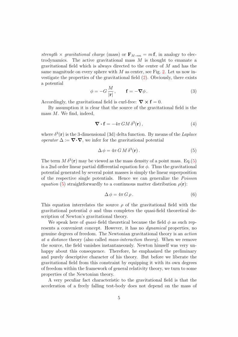
Figure 1: Two mass points m1 and m2 attracting each other in 3-dimensionalspace, Cartesian coordinates x, y, z.

M

m

rf

Figure 2: The “source” M attracts the test mass m.

4

strength × gravitational charge (mass) or FM→m = m f , in analogy to elec-trodynamics. The active gravitational mass M is thought to emanate agravitational field which is always directed to the center of M and has thesame magnitude on every sphere with M as center, see Fig. 2. Let us now in-vestigate the properties of the gravitational field (2). Obviously, there existsa potential

φ = −G M

|r|, f = −∇φ . (3)

Accordingly, the gravitational field is curl-free: ∇× f = 0.By assumption it is clear that the source of the gravitational field is the

mass M . We find, indeed,

∇ · f = −4π GM δ3(r) , (4)

where δ3(r) is the 3-dimensional (3d) delta function. By means of the Laplaceoperator ∆ :=∇·∇, we infer for the gravitational potential

∆φ = 4π GM δ3(r) . (5)

The term M δ3(r) may be viewed as the mass density of a point mass. Eq.(5)is a 2nd order linear partial differential equation for φ. Thus the gravitationalpotential generated by several point masses is simply the linear superpositionof the respective single potentials. Hence we can generalize the Poissonequation (5) straightforwardly to a continuous matter distribution ρ(r):

∆φ = 4π Gρ . (6)

This equation interrelates the source ρ of the gravitational field with thegravitational potential φ and thus completes the quasi-field theoretical de-scription of Newton’s gravitational theory.

We speak here of quasi–field theoretical because the field φ as such rep-resents a convenient concept. However, it has no dynamical properties, nogenuine degrees of freedom. The Newtonian gravitational theory is an actionat a distance theory (also called mass-interaction theory). When we removethe source, the field vanishes instantaneously. Newton himself was very un-happy about this consequence. Therefore, he emphasized the preliminaryand purely descriptive character of his theory. But before we liberate thegravitational field from this constraint by equipping it with its own degreesof freedom within the framework of general relativity theory, we turn to someproperties of the Newtonian theory.

A very peculiar fact characteristic to the gravitational field is that theacceleration of a freely falling test-body does not depend on the mass of

5

tidal accelerationtidal

acceleration

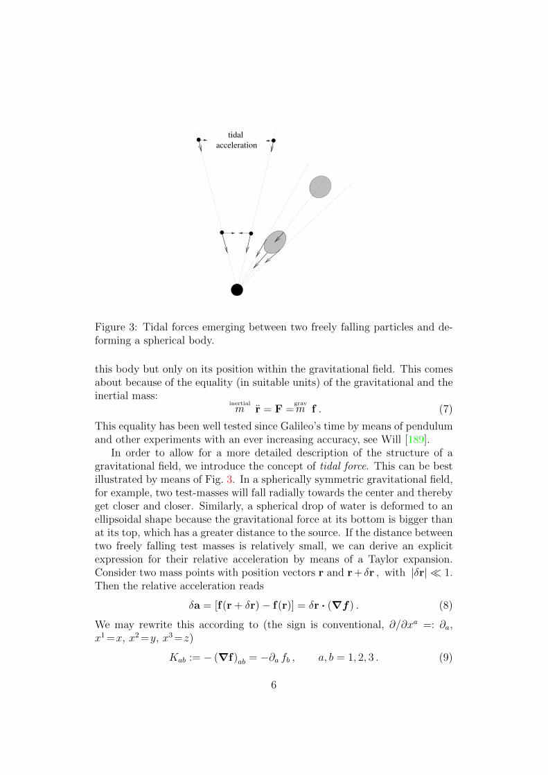
Figure 3: Tidal forces emerging between two freely falling particles and de-forming a spherical body.

this body but only on its position within the gravitational field. This comesabout because of the equality (in suitable units) of the gravitational and theinertial mass:

inertial

m r = F =grav

m f . (7)

This equality has been well tested since Galileo’s time by means of pendulumand other experiments with an ever increasing accuracy, see Will [189].

In order to allow for a more detailed description of the structure of agravitational field, we introduce the concept of tidal force. This can be bestillustrated by means of Fig. 3. In a spherically symmetric gravitational field,for example, two test-masses will fall radially towards the center and therebyget closer and closer. Similarly, a spherical drop of water is deformed to anellipsoidal shape because the gravitational force at its bottom is bigger thanat its top, which has a greater distance to the source. If the distance betweentwo freely falling test masses is relatively small, we can derive an explicitexpression for their relative acceleration by means of a Taylor expansion.Consider two mass points with position vectors r and r + δr , with |δr| 1.Then the relative acceleration reads

δa = [f(r + δr)− f(r)] = δr · (∇f) . (8)

We may rewrite this according to (the sign is conventional, ∂/∂xa =: ∂a,x1 =x, x2 =y, x3 =z)

Kab := − (∇f)ab = −∂a fb , a, b = 1, 2, 3 . (9)

6

We call Kab the tidal force matrix. The vanishing curl of the gravitationalfield is equivalent to its symmetry, Kab = Kba. Furthermore, Kab = ∂a ∂b φ.Thus, the Poisson equation becomes,

3∑a=1

Kaa = traceK = 4π Gρ . (10)

Accordingly, in vacuum Kab is trace-free.Let us now investigate the gravitational potential of a homogeneous star

with constant mass density ρ and total mass M = (4/3) π R3 ρ. For

our Sun, the radius is R = 6.9598 × 108 m and the total mass is M =1.989× 1030 kg.

Outside the sun (in the idealized picture we are using here), we havevacuum. Accordingly, ρ(r) = 0 for |r| > R. Then the Poisson equationreduces to the Laplace equation

∆φ = 0 , for r > R . (11)

In 3d polar coordinates, the r-dependent part of the Laplacian has the form(1/r2) ∂r (r2 ∂r). Thus (11) has the solution

φ =α

r+ β , (12)

where α and β are integration constants. Requiring that the potential tendsto zero as r goes to infinity, we get β = 0. The integration constant α willbe determined from the requirement that the force should change smoothlyas we cross the star’s surface, that is, the interior and exterior potential andtheir first derivatives have to be matched continuously at r = R.

Inside the star we have to solve

∆φ = 4π Gρ , for r ≤ R . (13)

We find

φ =2

3πGρ r

2 +C1

r+ C2 , (14)

with integration constants C1 and C2. We demand that the potential in thecenter r = 0 has a finite value, say φ0. This requires C1=0. Thus

φ =2

3π Gρ r

2 + φ0 =GM(r)

2r+ φ0 , (15)

where we introduced the mass function M(r) = (4/3) πr3ρ which measuresthe total mass inside a sphere of radius r.

7

interiorR0

φ

∼ r2

φ0−

∼ 1r

∞rexterior −→

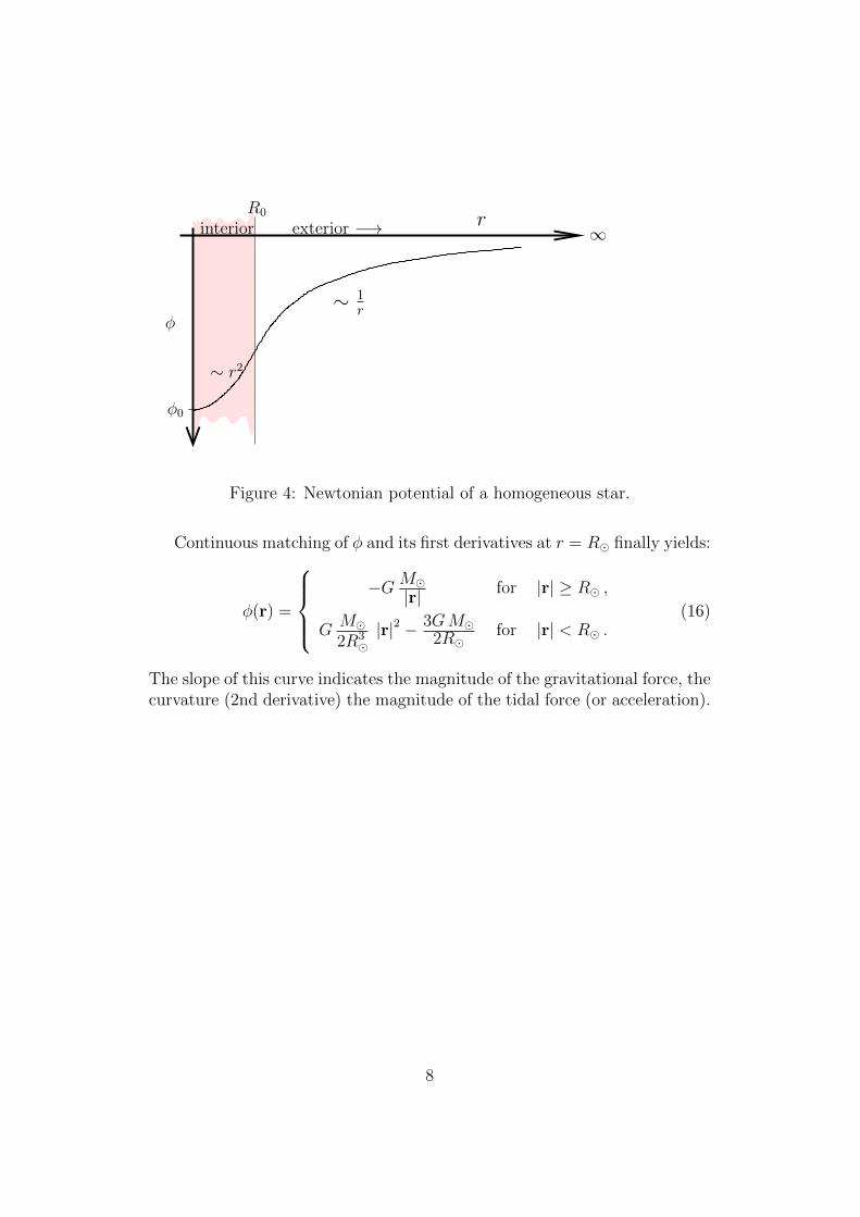
Figure 4: Newtonian potential of a homogeneous star.

Continuous matching of φ and its first derivatives at r = R finally yields:

φ(r) =

−G M

|r| for |r| ≥ R ,

GM2R3|r|2 − 3GM

2Rfor |r| < R .

(16)

The slope of this curve indicates the magnitude of the gravitational force, thecurvature (2nd derivative) the magnitude of the tidal force (or acceleration).

8

1.2 Minkowski space

When, in a physical experiment, gravity can be safely neglected, we seem tolive in the flat Minkowski space of special relativity theory. We introducethe metric of the Minkowksi space and rewrite it in terms of so-called nullcoordinates, that is, we use light rays for a parametrization of Minkowskispace.

Henceforth space by itself, and time by itself, are doomed tofade away into mere shadows, and only a kind of union ofthe two will preserve an independent reality.

Hermann Minkowski (1908)

It was Minkowski who welded space and time together into spacetime,thereby abandoning the observer-independent meaning of spatial and tem-poral distances. Instead, the spatio-temporal distance, the line element,

ds2 = −c2 dt2 + dx2 + dy2 + dz2

is distinguished as the invariant measure of spacetime. The Poincare (orinhomogeneous Lorentz) transformations form the invariance group of thisspacetime metric. The principle of the constancy of the speed of light isembodied in the equation ds2 = 0. Suppressing one spatial dimension, thesolutions of this equation can be regarded as a double cone. This light conevisualizes the paths of all possible light rays arriving at or emitted fromthe cone’s apex. Picturing the light cone structure, and thereby the causalproperties of spacetime, will be our method for analyzing the meaning of theSchwarzschild and the Kerr solution.

Null coordinates

We first introduce so-called null coordinates. The Minkowski metric (withc = 1), in spherical polar coordinates reads

ds2 = −dt2 + dr2 + r2(dθ2 + sin2 θ dφ2

)= −dt2 + dr2 + r2 dΩ2 . (17)

We define advanced and retarded null coordinates according to

v := t+ r , u := t− r , (18)

and find

ds2 = −dv du+1

4(v − u)2 dΩ2 . (19)

9

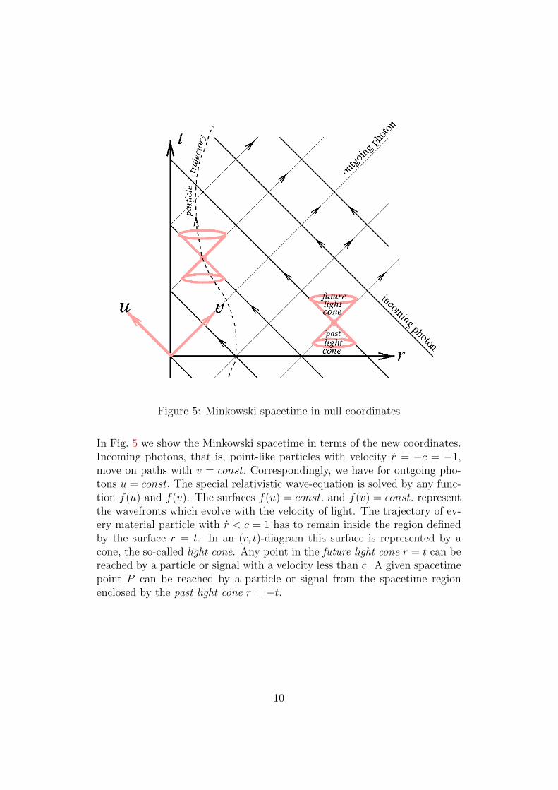
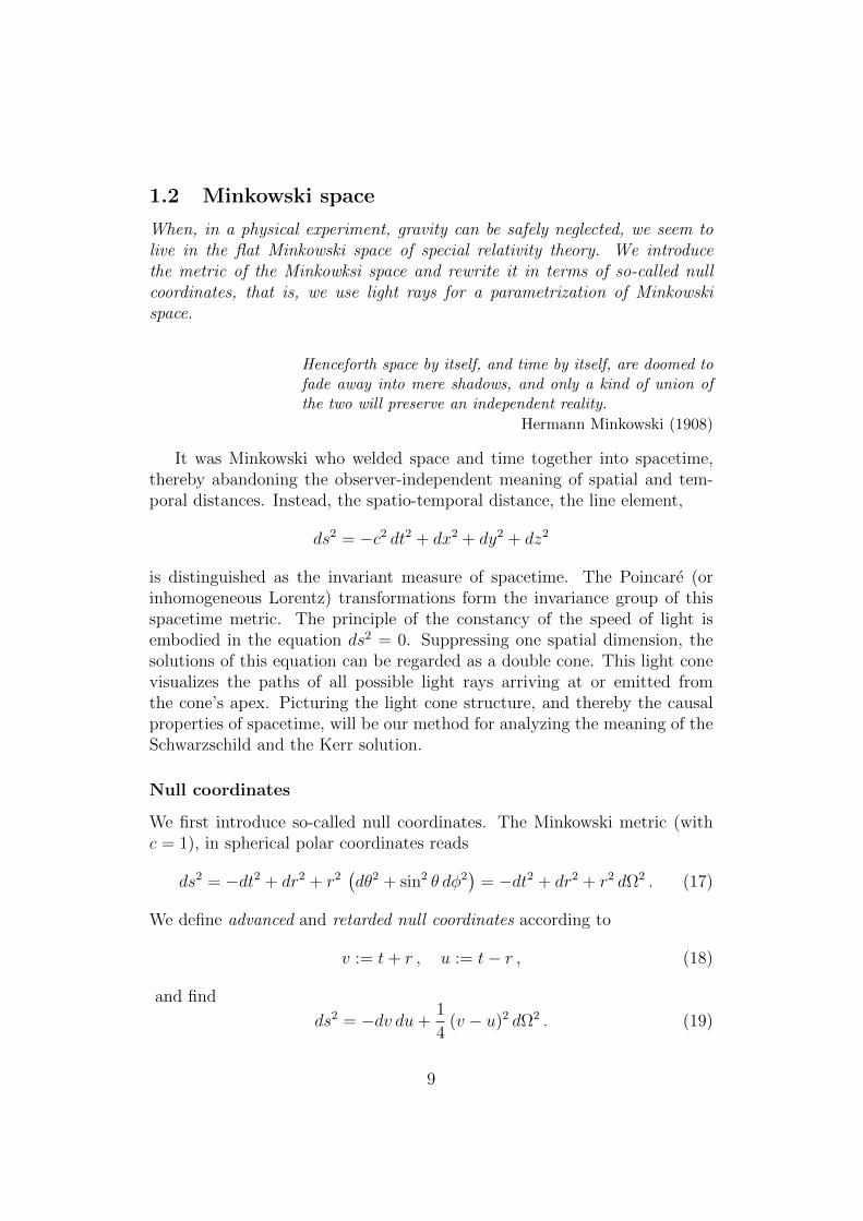
Figure 5: Minkowski spacetime in null coordinates

In Fig. 5 we show the Minkowski spacetime in terms of the new coordinates.Incoming photons, that is, point-like particles with velocity r = −c = −1,move on paths with v = const. Correspondingly, we have for outgoing pho-tons u = const. The special relativistic wave-equation is solved by any func-tion f(u) and f(v). The surfaces f(u) = const. and f(v) = const. representthe wavefronts which evolve with the velocity of light. The trajectory of ev-ery material particle with r < c = 1 has to remain inside the region definedby the surface r = t. In an (r, t)-diagram this surface is represented by acone, the so-called light cone. Any point in the future light cone r = t can bereached by a particle or signal with a velocity less than c. A given spacetimepoint P can be reached by a particle or signal from the spacetime regionenclosed by the past light cone r = −t.

10

Penrose diagram

We can map, following Penrose, the infinitely distant points of spacetime intofinite regions by means of a conformal transformation which leaves the lightcones intact. Then we can display the whole infinite Minkowski spacetimeon a (finite) piece of paper. Accordingly, introduce the new coordinates

v := arctan v , u := arctan u , for − π/2 ≤ (v , u) ≤ +π/2 . (20)

Then the metric reads

ds2 =1

cos2 v

1

cos2 u

[−dv du+

1

4sin2 (v − u) dΩ2

]. (21)

We can go back to time- and space-like coordinates by means of the trans-formation

t := v + u , r := v − u , (22)

see (18). Then the metric reads,

ds2 =−dt2 + dr2 + sin2 r dΩ2

4 cos2 t+r2

cos2 t−r2

, (23)

that is, up to the function in the denominator, it appears as a flat metric.Such a metric is called conformally flat (it is conformal to a static Einsteincosmos). The back-transformation to our good old Minkowski coordinatesreads

t =1

2

(tan

t+ r

2+ tan

t− r2

), (24)

r =1

2

(tan

t+ r

2− tan

t− r2

). (25)

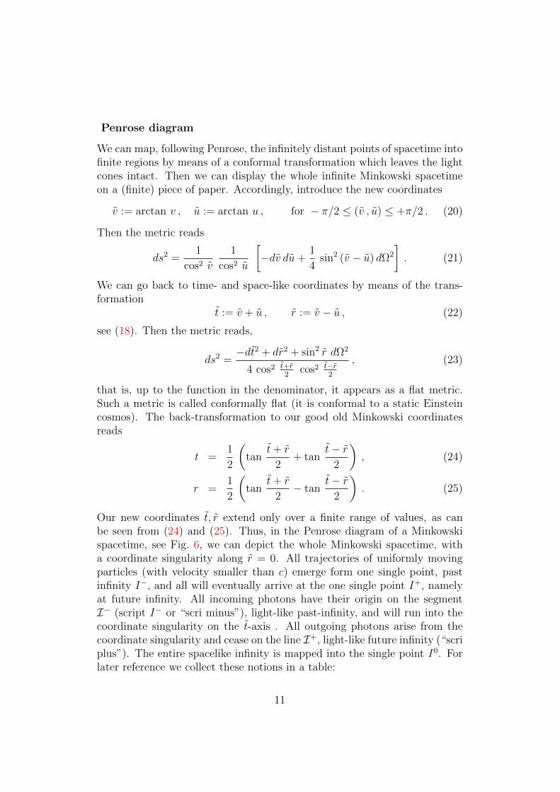
Our new coordinates t, r extend only over a finite range of values, as canbe seen from (24) and (25). Thus, in the Penrose diagram of a Minkowskispacetime, see Fig. 6, we can depict the whole Minkowski spacetime, witha coordinate singularity along r = 0. All trajectories of uniformly movingparticles (with velocity smaller than c) emerge form one single point, pastinfinity I−, and all will eventually arrive at the one single point I+, namelyat future infinity. All incoming photons have their origin on the segmentI− (script I− or “scri minus”), light-like past-infinity, and will run into thecoordinate singularity on the t-axis . All outgoing photons arise from thecoordinate singularity and cease on the line I+, light-like future infinity (“scriplus”). The entire spacelike infinity is mapped into the single point I0. Forlater reference we collect these notions in a table:

11

−πI−

+πI+

+π

I0

I+

I−

t

r

r = const

t = const

light cone

light cone

coor

din

ate

singu

lari

ty

Figure 6: Penrose diagram of Minkowski spacetime.

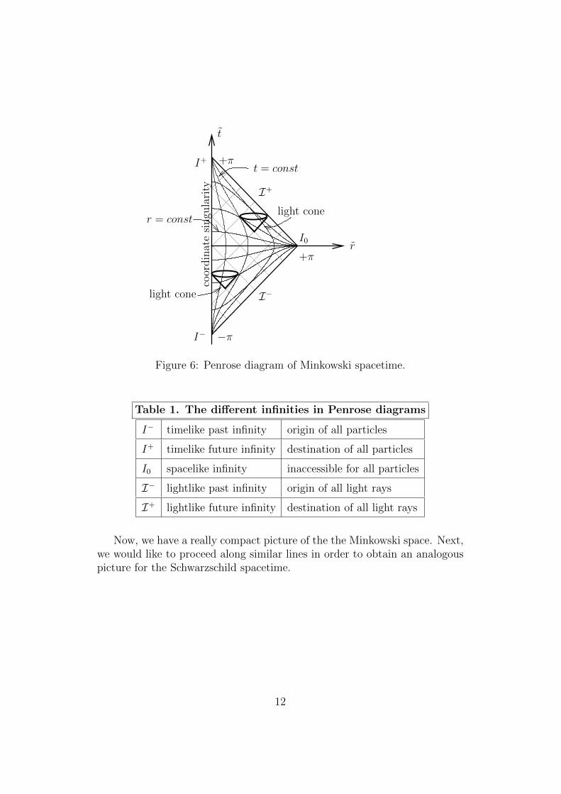
Table 1. The different infinities in Penrose diagrams

I− timelike past infinity origin of all particles

I+ timelike future infinity destination of all particles

I0 spacelike infinity inaccessible for all particles

I− lightlike past infinity origin of all light rays

I+ lightlike future infinity destination of all light rays

Now, we have a really compact picture of the the Minkowski space. Next,we would like to proceed along similar lines in order to obtain an analogouspicture for the Schwarzschild spacetime.

12

1.3 Einstein’s field equation

We display our notations and conventions for the differential geometric toolsused to formulate Einstein’s field equation.

We assume that our readers know at least the rudiments of general relativ-ity (GR) as represented, for instance, in Einstein’s Meaning of Relativity[50],which we still recommend as a gentle introduction into GR. More advancedreaders may then want to turn to Rindler[165] and/or to Landau-Lifshitz[106].

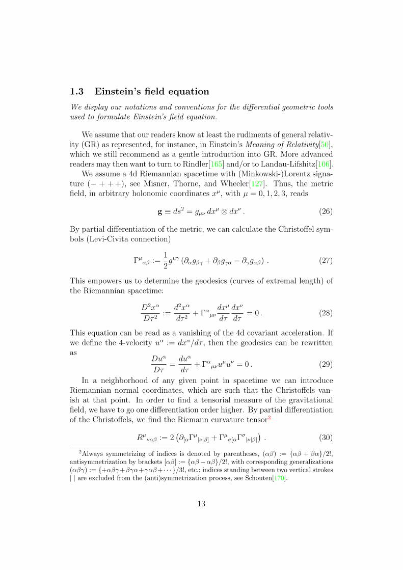
We assume a 4d Riemannian spacetime with (Minkowski-)Lorentz signa-ture (− + + +), see Misner, Thorne, and Wheeler[127]. Thus, the metricfield, in arbitrary holonomic coordinates xµ, with µ = 0, 1, 2, 3, reads

g ≡ ds2 = gµν dxµ ⊗ dxν . (26)

By partial differentiation of the metric, we can calculate the Christoffel sym-bols (Levi-Civita connection)

Γµαβ :=1

2gµγ (∂αgβγ + ∂βgγα − ∂γgαβ) . (27)

This empowers us to determine the geodesics (curves of extremal length) ofthe Riemannian spacetime:

D2xα

Dτ 2:=

d2xα

dτ 2+ Γαµν

dxµ

dτ

dxν

dτ= 0 . (28)

This equation can be read as a vanishing of the 4d covariant acceleration. Ifwe define the 4-velocity uα := dxα/dτ , then the geodesics can be rewrittenas

Duα

Dτ=duα

dτ+ Γαµνu

µuν = 0 . (29)

In a neighborhood of any given point in spacetime we can introduceRiemannian normal coordinates, which are such that the Christoffels van-ish at that point. In order to find a tensorial measure of the gravitationalfield, we have to go one differentiation order higher. By partial differentiationof the Christoffels, we find the Riemann curvature tensor2

Rµναβ := 2

(∂[αΓµ|ν|β] + Γµσ[αΓσ |ν|β]

). (30)

2Always symmetrizing of indices is denoted by parentheses, (αβ) := αβ + βα/2!,antisymmetrization by brackets [αβ] := αβ−αβ/2!, with corresponding generalizations(αβγ) := +αβγ+βγα+γαβ+ · · · /3!, etc.; indices standing between two vertical strokes| | are excluded from the (anti)symmetrization process, see Schouten[170].

13

The curvature is doubly antisymmetric, its two index pairs commute, and itstotally antisymmetric piece vanishes:

R(µν)αβ = 0 , Rµν(αβ) = 0 ; Rµναβ = Rαβµν ; R[µναβ] = 0 . (31)

If we define collective indices A,B, .. = 1, ..., 6 for the antisymmetric indexpairs according to the rule 01, 02, 03; 23, 31, 12 −→ 1, 2, 3; 4, 5, 6, thenthe algebraic symmetries of (31) can be rephrased as

RAB = RBA , trace(RAB) = 0. (32)

Thus, in 4d the curvature can be represented as a trace-free symmetric 6×6-matrix. Hence it has 20 independent components.

With the curvature tensor, we found a tensorial measure for the grav-itational field. Freely falling particles move along geodesics of Riemannianspacetime. What about the tidal accelerations between two freely falling par-ticles? Let the “infinitesimal” vector nα describe the distance between twoparticles moving on adjacent geodesics. A standard calculation[127], linearto the order of n, yields the geodesic deviation equation

D2nα

Dτ 2= uβuγRα

βγδ nδ . (33)

This equation describes the relative acceleration of neighboring particles,similar as (8) and (9) in the Newtonian case. The role of the tidal matrixKab is taken over by Kαδ := uβuγRα

βγδ.By contraction of the curvature, we can define the 2nd rank Ricci tensor

Rµν and the curvature scalar R, respectively:

Rµν := Rαµαν , R := gµνRµν . (34)

For convenience, we can also introduce the Einstein tensor Gµν := Rµν −12gµνR. The curvature with its 20 independent components can be irreducibly

decomposed into smaller pieces according to 20 = 10 + 9 + 1. The Weylcurvature tensor Cαβγδ is trace-free and has 10 independent components,whereas the trace-free Ricci tensor has 9 components and the curvature scalarjust 1.

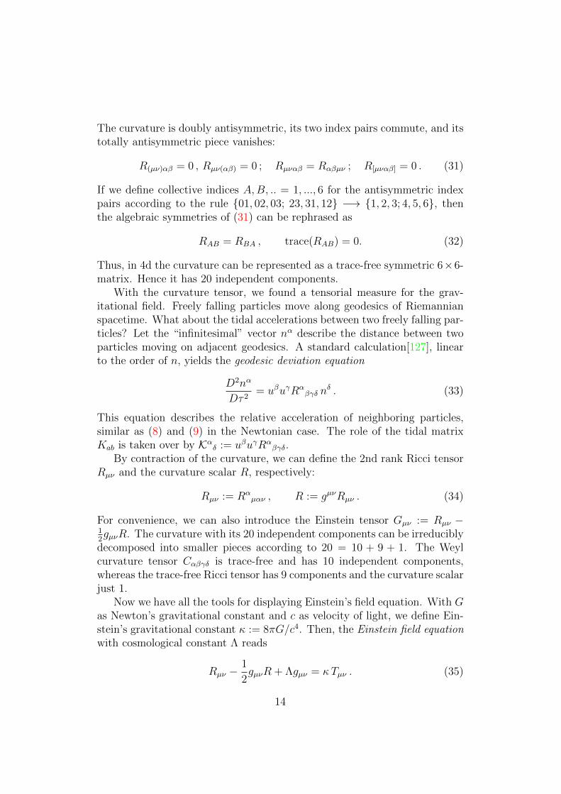
Now we have all the tools for displaying Einstein’s field equation. With Gas Newton’s gravitational constant and c as velocity of light, we define Ein-stein’s gravitational constant κ := 8πG/c4. Then, the Einstein field equationwith cosmological constant Λ reads

Rµν −1

2gµνR + Λgµν = κTµν . (35)

14

The source on the right-hand side is the energy-momentum tensor of matter.The vacuum field equation, without cosmological constant, simply reduces toRµν = 0. Mostly this equation will keep us busy in this article. A vanishingRicci tensor implies that only the Weyl curvature Cαβγδ 6= 0. Accordingly,the vacuum field in GR (without Λ) is represented by the Weyl tensor.

Eq.(35) represents a generalization of the Poisson equation (10). There,the contraction of the tidal matrix is proportional to the mass density; inGR, the contraction of the curvature tensor is proportional to the energy-momentum tensor.

The physical mass is denoted by M . Usually, we use the mass parameter,m := GM

c2. The Schwarzschild radius reads rS := 2m = 2GM

c2. Usually we put

c = 1 and G = 1. We make explicitly use of G and c as soon as we stressanalogies to Newtonian gravity or allude to observational data.

15

2 The Schwarzschild metric (1916)

Spatial spherical symmetry is assumed and a corresponding exact solutionfor Einstein’s theory searched for. After a historical outline (Sec.2.1), weapply the equivalence principle to a freely falling particle and try to imple-ment that on top of the Minkowskian line element. In this way, we heuristi-cally arrive at the Schwarzschild metric (Sec.2.2). In Sec.2.3, we display theSchwarzschild metric in six different classical coordinate systems. We out-line the concept of a Schwarzschild black hole in Sec.2.4. In Secs.2.5 and 2.6,we construct the Penrose diagram for the Schwarzschild(-Kruskal) spacetime.We add electric charge to the Schwarzschild solution in Sec.2.7. The interiorSchwarzschild metric, with matter, is addressed in Sec.2.8.

It is quite a wonderful thing that from such an abstractidea the explanation of the Mercury anomaly emerges so in-evitably.

Karl Schwarzschild[171] (1915)

2.1 Historical remarks

The genesis of the Schwarzschild solution (1915/16) is described. In par-ticular, we show that Droste, a bit later than Schwarzschild, arrived at theSchwarzschild metric independently. He put the Schwarzschild solution intothat form in which we use it today.

The first exact solution of Einstein’s field equation was born in hospi-tal. Unfortunately, the circumstances were more tragic than joyful. Theastronomer Karl Schwarzschild joined the German army right at the begin-ning of World War I and served in Belgium, France, and Russia. At theend of the year 1915, he was admitted to hospital with an acute skin dis-ease. There, not far from the Russian front, enduring the distant gunfire,he found time to “stroll through the land of ideas” of Einstein’s theory,as he puts it in a letter to Einstein3 dated 22 December 1915. Accordingto this letter, Schwarzschild started out from the approximate solution inEinstein’s “perihelion paper”, published November 25th. Since presumablyletters from Berlin to the Russian front took a few days, Schwarzschild[172]found the solution within about a fortnight. Fortunately, the premature fieldequation of the “perihelion paper” is correct in the vacuum case treated bySchwarzschild.

3 The letters from and to Einstein can be found in Einstein’s Collected Works[51], seealso Schwarzschild’s Collected Works[171].

16

In February 1916, Schwarzschild[173] submitted the spherically symmet-ric solution with matter—the “interior Schwarzschild solution”—now basedon Einstein’s final field equation. In March 1916, he was sent home were hepassed away on 11 May 1916.

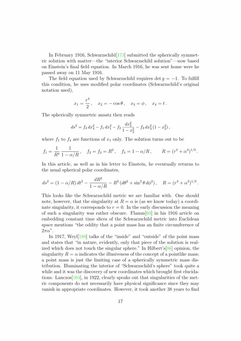
The field equation used by Schwarzschild requires det g = −1. To fulfillthis condition, he uses modified polar coordinates (Schwarzschild’s originalnotation used),

x1 =r3

2, x2 = − cos θ , x3 = φ , x4 = t .

The spherically symmetric ansatz then reads

ds2 = f4 dx24 − f1 dx

21 − f2

dx22

1− x22

− f3 dx23 (1− x2

2) ,

where f1 to f4 are functions of x1 only. The solution turns out to be

f1 =1

R4

1

1− α/R, f2 = f3 = R2 , f4 = 1− α/R , R = (r3 + α3)1/3 .

In this article, as well as in his letter to Einstein, he eventually returns tothe usual spherical polar coordinates,

ds2 = (1− α/R) dt2 − dR2

1− α/R−R2 (dθ2 + sin2 θ dφ2) , R = (r3 + α3)1/3 .

This looks like the Schwarzschild metric we are familiar with. One shouldnote, however, that the singularity at R = α is (as we know today) a coordi-nate singularity, it corresponds to r = 0. In the early discussion the meaningof such a singularity was rather obscure. Flamm[60] in his 1916 article onembedding constant time slices of the Schwarzschild metric into Euclideanspace mentions “the oddity that a point mass has an finite circumference of2πα”.

In 1917, Weyl[188] talks of the “inside” and “outside” of the point massand states that “in nature, evidently, only that piece of the solution is real-ized which does not touch the singular sphere.” In Hilbert’s[86] opinion, thesingularity R = α indicates the illusiveness of the concept of a pointlike mass;a point mass is just the limiting case of a spherically symmetric mass dis-tribution. Illuminating the interior of “Schwarzschild’s sphere” took quite awhile and it was the discovery of new coordinates which brought first elucida-tions. Lanczos[104], in 1922, clearly speaks out that singularities of the met-ric components do not necessarily have physical significance since they mayvanish in appropriate coordinates. However, it took another 38 years to find

17

a maximally extended fully regular coordinate system for the Schwarzschildmetric. We will become acquainted with these Kruskal/Szekeres coordinatesin Sec.2.5.

Schwarzschild’s solution, published in the widely read minutes of thePrussian Academy, communicated by Einstein himself, nearly instantly trig-gered further investigations of the gravitational field of a point mass. Alreadyin March 1916, Reissner[163], a civil engineer by education, published a gen-eralization of the Schwarzschild metric, including an electrical charge; thiswas later completed by Weyl[188] and by Nordstrom[140]. Today it is calledReissner-Nordstrom solution.

Nevertheless, one should not ignore the Dutch twin of Schwarzschild’ssolution. On 27 May 1916, Droste[47] communicated his results on “thefield of a single centre in Einstein’s theory of gravitation, and the motionof a particle in that field” to the Dutch Academy of Sciences. He presentsa very clear and easy to read derivation of the metric and gives a quitecomprehensive analysis of the motion of a point particle. Since 1913, he hadbeen working on general relativity under the supervision of Lorentz at LeidenUniversity. Published in Dutch, Droste’s results are fairly unknown today.Einstein, probably informed by his close friend Ehrenfest, rather appreciatedDroste’s work, praising the graceful mathematical style. Weyl[188] also citesDroste, but in Hilbert’s[86] second communication the reference is not found.Einstein, Hilbert, and Weyl always allude to “Schwarzschild’s solution”.

After Droste took his PhD in 1916, he worked as school teacher andeventually became professor for mathematics in Leiden. He never resumed hiswork on Einstein’s theory and his name faded from the relativistic memoirs.In Leiden, people like Lorentz, de Sitter, Nordstrom, or Fokker learned aboutthe gravitational field of a point mass primarily from Droste’s work. Thus,the name “Schwarzschild–Droste solution” would be quite justified from ahistorical point of view.

The importance of the Schwarzschild metric is made evident by the Birk-hoff[16] theorem4: For vanishing cosmological constant, the unique spheri-cally symmetric vacuum spacetime is the Schwarzschild solution, which canbe expressed most conveniently in Schwarzschild coordinates, see Table 3,entry 1. Thus, a spherically symmetric body is static (outside the horizon).In particular, it cannot emit gravitational radiation. Moreover, the asymp-totic Minkowskian behavior of the Schwarzschild solution is dictated by thesolution itself, it is not imposed from the outside.

4The “Birkhoff” theorem was discovered by Jebsen[95], Birkhoff[16], andAlexandrow[4]. For more details on Jebsen, see Johansen & Ravndal[96]. The objectionsof Ehlers & Krasinski[48] appear to us as nitpicking.

18

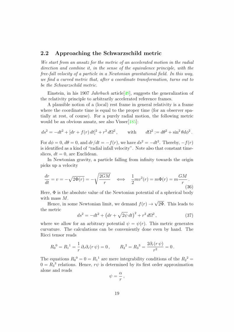
2.2 Approaching the Schwarzschild metric

We start from an ansatz for the metric of an accelerated motion in the radialdirection and combine it, in the sense of the equivalence principle, with thefree-fall velocity of a particle in a Newtonian gravitational field. In this way,we find a curved metric that, after a coordinate transformation, turns out tobe the Schwarzschild metric.

Einstein, in his 1907 Jahrbuch article[49], suggests the generalization ofthe relativity principle to arbitrarily accelerated reference frames.

A plausible notion of a (local) rest frame in general relativity is a framewhere the coordinate time is equal to the proper time (for an observer spa-tially at rest, of course). For a purely radial motion, the following metricwould be an obvious ansatz, see also Visser[185]:

ds2 = −dt2 + [dr + f(r) dt]2 + r2 dΩ2 , with dΩ2 := dθ2 + sin2 θdφ2 .

For dφ = 0, dθ = 0, and dr/dt = −f(r), we have ds2 = −dt2. Thereby, −f(r)is identified as a kind of “radial infall velocity”. Note also that constant time-slices, dt = 0, are Euclidean.

In Newtonian gravity, a particle falling from infinity towards the originpicks up a velocity

dr

dt= v = −

√2Φ(r) = −

√2GM

r⇐⇒ 1

2mv2(r) = mΦ(r) = m

GM

r.

(36)Here, Φ is the absolute value of the Newtonian potential of a spherical bodywith mass M .

Hence, in some Newtonian limit, we demand f(r)→√

2Φ. This leads tothe metric

ds2 = −dt2 +(dr +

√2ψ dt

)2+ r2 dΩ2 , (37)

where we allow for an arbitrary potential ψ = ψ(r). This metric generatescurvature. The calculations can be conveniently done even by hand. TheRicci tensor reads

R00 = R1

1 =1

r∂r∂r(r ψ) = 0 , R2

2 = R33 =

2∂r(r ψ)

r2= 0 .

The equations R00 = 0 = R1

1 are mere integrability conditions of the R22 =

0 = R33 relations. Hence, rψ is determined by its first order approximation

alone and readsψ =

α

r,

19

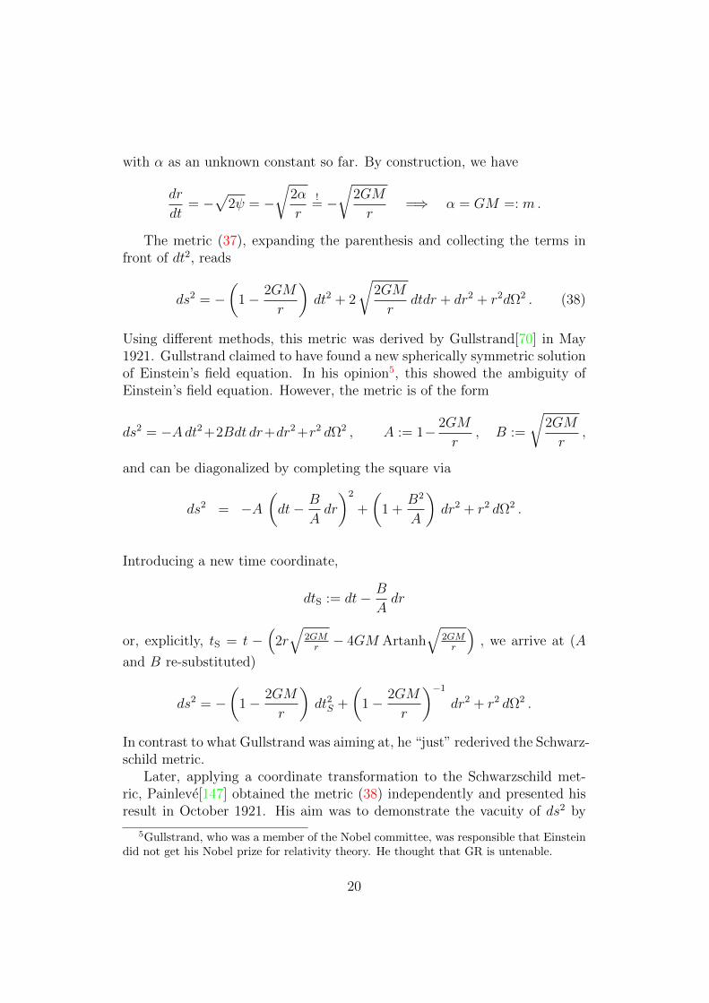
with α as an unknown constant so far. By construction, we have

dr

dt= −

√2ψ = −

√2α

r!

= −√

2GM

r=⇒ α = GM =: m.

The metric (37), expanding the parenthesis and collecting the terms infront of dt2, reads

ds2 = −(

1− 2GM

r

)dt2 + 2

√2GM

rdtdr + dr2 + r2dΩ2 . (38)

Using different methods, this metric was derived by Gullstrand[70] in May1921. Gullstrand claimed to have found a new spherically symmetric solutionof Einstein’s field equation. In his opinion5, this showed the ambiguity ofEinstein’s field equation. However, the metric is of the form

ds2 = −Adt2 +2Bdt dr+dr2 +r2 dΩ2 , A := 1− 2GM

r, B :=

√2GM

r,

and can be diagonalized by completing the square via

ds2 = −A(dt− B

Adr

)2

+

(1 +

B2

A

)dr2 + r2 dΩ2 .

Introducing a new time coordinate,

dtS := dt− B

Adr

or, explicitly, tS = t −(

2r√

2GMr− 4GM Artanh

√2GMr

), we arrive at (A

and B re-substituted)

ds2 = −(

1− 2GM

r

)dt2S +

(1− 2GM

r

)−1

dr2 + r2 dΩ2 .

In contrast to what Gullstrand was aiming at, he “just” rederived the Schwarz-schild metric.

Later, applying a coordinate transformation to the Schwarzschild met-ric, Painleve[147] obtained the metric (38) independently and presented hisresult in October 1921. His aim was to demonstrate the vacuity of ds2 by

5Gullstrand, who was a member of the Nobel committee, was responsible that Einsteindid not get his Nobel prize for relativity theory. He thought that GR is untenable.

20

showing that an exact solution does not determine the physical geometryand is therefore meaningless. In a letter (Dec. 7th 1921) to Painleve, Ein-stein stresses on the contrary the meaninglessness of the coordinates! In thewords of Einstein himself (our translation): “. . . merely results obtained byeliminating the coordinate dependence can claim an objective meaning.”

In the subsequent section, we will meet the Schwarzschild metric in manydifferent coordinate systems. All of them have their merits and their short-comings.

Using Gullstrand-Painleve coordinates for the Schwarzschild metric doesnot change the physics, of course. However, as a coordinate system it is whatGustav Mie[126] calls a sensible coordinate system. In contrast to manyother coordinate systems, the physics looks quite like we are used to. As anexample, we analyze the motion of a radial infalling particle in Schwarzschildand Gullstrand-Painleve coordinates.

The equations of motion for point particles in general relativity are ob-tained via the geodesic equation (28). It can be shown that this equa-tion is equivalent to the solution of the variational principle δ

∫xαds2 =

δ∫xα xβ gαβ dτ

2. We choose the proper time τ for the parametrization ofthe curve, the dot denotes the derivative with respect to τ . In the present con-text, we are only interested in the velocity of particles along ingoing geodesics(“freely falling particles”). For time-like geodesics we have −1 = ds2

dτ2. This

allows the algebraic determination of r provided we know t. Since we con-

sider static metrics here, t is a cyclic variable and(∂∂t

ds2

dτ2

)= K = const.

The constant is determined by the boundary condition r = 0 for r → ∞.The calculation yields:

Table 2. Velocities in different coordinate systems6

Schwarzschild Gullstrand-Painlevecoordinate

velocitydrdt

±(1− 2GM

r

)√2GMr −

√2GMr

particlespropervelocity

drdτ

±√

2GMr ±

√2GMr

light rays

coordinatevelocity

drdt

±(1− 2GMr ) ±1−

√2GMr

6The velocities of outgoing particles are valid only for the boundary condition specified.The coordinate velocity for outgoing particles in GP coordinates does not fit in our tableand is thus suppressed.

21

The difference between the coordinate systems appears in the first lineof Table 2: In Gullstrand-Painleve coordinates, the coordinate velocity of afreely infalling particle increases smoothly towards the center. Nothing spe-cial happens at r = 2GM . From a given position, the particle will plunge intothe center in a finite time. Even numerically this looks quite Newtonian. Incontrast, the velocity with respect to Schwarzschild coordinates approacheszero as the particle approaches r = 2GM . Hence, the particle apparentlywill not be able to go further than r = 2GM .

For the Gullstrand-Painleve metric for incoming light the radial coordi-nate velocity is always larger in magnitude than −1, at r = 2GM it is −2,for outgoing rays it vanishes at r = 2GM and is negative for r < 2GM .

Taking the mere numerical values is misleading. Contemplate for incom-ing light (

drdt

)particle(

drdt

)light

=1

1 +√

r2GM

≤ 1 .

So the particle is always slower than light, however it approaches the velocityof light when approaching r = 0.

The Gullstrand-Painleve form of the metric is regular at the surface r =2GM . This shows that it is not any kind of barrier, but this observation wasnot made until much later, see Eisenstaedt [52].

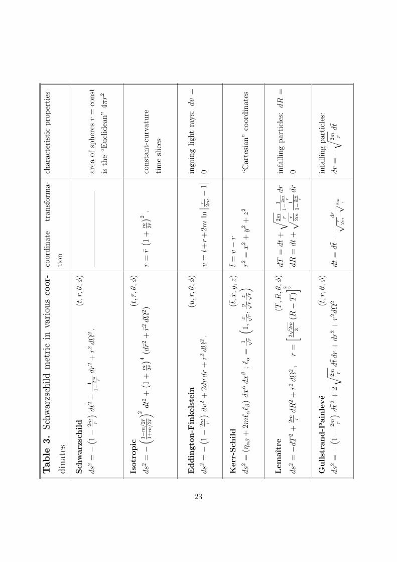
2.3 Six classical representations of the Schwarzschildmetric

As we mentioned, a coordinate system should be chosen according to its con-venience for describing a certain situation. In the following table (Table 3),we collect six widely used forms of the Schwarzschild metric.

22

Tab

le3.

Sch

war

zsch

ild

met

ric

inva

riou

sco

or-

din

ates

coor

din

ate

tran

sfor

ma-

tion

char

acte

rist

icpro

per

ties

Sch

warz

schild

(t,r,θ,φ

)

ds2

=−( 1−

2m r

) dt2+

11−

2m r

dr2

+r2dΩ

2.

area

ofsp

her

esr

=co

nst

isth

e“E

ucl

idea

n”

4πr2

Isotr

op

ic(t,r,θ,φ

)

ds2

=−( 1−m/2r

1+m/2r

) 2 dt2

+( 1

+m 2r

) 4 (dr2

+r2dΩ

2)

r=r( 1

+m 2r

) 2 .co

nst

ant-

curv

ature

tim

esl

ices

Eddin

gto

n-F

inkels

tein

(u,r,θ,φ

)

ds2

=−( 1−

2m r

) dv2+

2dvdr

+r2dΩ

2.

v=t+r+

2mln∣ ∣r 2m−

1∣ ∣ingo

ing

ligh

tra

ys:dv

=

0

Kerr

-Sch

ild

(t,x,y,z

)

ds2

=(ηαβ

+2m

` α` β

)dxαdxβ

;` α

=1 √r

( 1,x √r,y √rz √r

)t

=v−r

r2=x

2+y

2+z2

“Car

tesi

an”

coor

din

ates

Lem

aıt

re(T,R,θ,φ

)

ds2

=−dT

2+

2m rdR

2+r2dΩ

2,

r=[ 2√

2m

3(R−T

)]2 3

dT

=dt

+√ 2

m r1

1−

2m r

dr

dR

=dt

+√ r 2

m1

1−

2m r

dr

infa

llin

gpar

ticl

es:dR

=

0

Gullst

ran

d-P

ain

leve

(t,r,θ,φ

)

ds2

=−( 1−

2m r

) dt2+

2√ 2

m rdtdr

+dr2

+r2dΩ

2dt

=dt−

dr

√r

2m−√

2m r

infa

llin

gpar

ticl

es:

dr

=−√ 2

m rdt

23

2.4 The concept of a Schwarzschild black hole

We first draw a simple picture of a black hole. The event horizon and thestationary limit emerge as characteristic features. These are subsequentlydefined in a more mathematical way.

In 1783 John Michell communicated his thoughts on the means of dis-covering the Distance, magnitude, etc. of the fixed stars, in consequence ofthe diminuation of the velocity of their light . . . [125] to the Royal Societyin London. In the context of Newton’s particle theory of light, he calcu-lated that sufficiently massive stars exhibit a gravitational attraction to suchvast an amount that even light could not escape. A few years later (1796)Pierre-Simon Laplace published similar ideas.

In modern notation, we may reconstruct the arguments as follows. Wethrow a mass m from the surface of the Earth, assuming that there were noair, in upward direction with an initial velocity v. It will always fall back,unless its initial velocity reaches a sufficiently high value vescape providingthe mass with such a kinetic energy that it can overpower the gravitationalattraction of the Earth. Energy conservation yields then immediately theformula

vescape =

√2GM⊕R⊕

,

where G is Newton’s gravitational constant and M and R⊕ the mass and theradius of the spherically conceived Earth, respectively.

For the Earth we find vescape ≈ 11.2 km/s. If we now compress the Earthappreciably (thought experiment!) until the escape velocity coincides withthe speed of light vescape = c, its compressed “Schwarzschild” radius becomesr⊕ = 2GM⊕/c

2 ≈ 1 cm. For the Sun, with its mass M, we have7

r =2GMc2

≈ 3 km .

At any smaller radius the light will be confined to the corresponding body.This is an intuitive picture of a spherically symmetric invisible “black hole”.8

It is very intriguing to see how far-sighted Michell anticipated the statusof today’s observational black hole physics:

7For the sake of clarity, we display here the speed of light c explicitly.8The phrase “black hole” is commonly associated with Wheeler (1968). It appears

definitely earlier in the literature: In the January 1964 edition of the Science News Letterthe journalist Ann Ewing entitled her report at the meeting of the American Associationfor the Advancement of Science in Cleveland “Black Holes” in space. And if you havea look into an arbitrary English language dictionary published before ca. 1970, you willlearn that “black hole” refers to a notorious dungeon in Calcutta (now Kolkata) in the18th century, apparently a place of no return . . .

24

If there should really exist in nature bodies, whose density is not less than that

of the sun, and whose diameters are more than 500 times the diameter of the sun,

since their light could not arrive at us; [. . . ] we could have no information from

sight; yet, if any other luminous bodies should happen to revolve about them we

might still perhaps from the motions of these revolving bodies infer the existence

of the central ones with some degree of probability . . .

This could be a verdict on the current observations of the black hole SgrA∗ (“Sagittarius A-star”) in the center of our Milky Way—and this is not athought experiment—for a popular account, see Sanders[168]. Sgr A∗ has amass of about 4 × 106M. Thus its Schwarzschild radius is far from beingminute, it is about 3× 4× 106 km or about 17 solar radii.

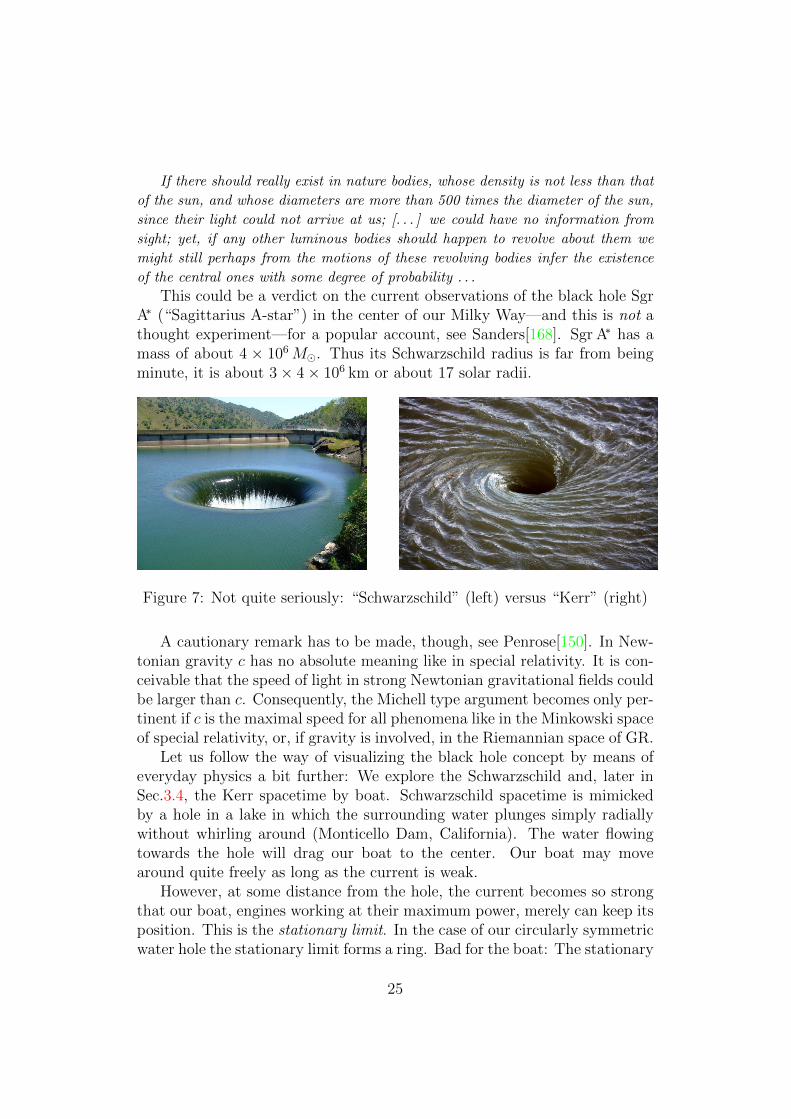
Figure 7: Not quite seriously: “Schwarzschild” (left) versus “Kerr” (right)

A cautionary remark has to be made, though, see Penrose[150]. In New-tonian gravity c has no absolute meaning like in special relativity. It is con-ceivable that the speed of light in strong Newtonian gravitational fields couldbe larger than c. Consequently, the Michell type argument becomes only per-tinent if c is the maximal speed for all phenomena like in the Minkowski spaceof special relativity, or, if gravity is involved, in the Riemannian space of GR.

Let us follow the way of visualizing the black hole concept by means ofeveryday physics a bit further: We explore the Schwarzschild and, later inSec.3.4, the Kerr spacetime by boat. Schwarzschild spacetime is mimickedby a hole in a lake in which the surrounding water plunges simply radiallywithout whirling around (Monticello Dam, California). The water flowingtowards the hole will drag our boat to the center. Our boat may movearound quite freely as long as the current is weak.

However, at some distance from the hole, the current becomes so strongthat our boat, engines working at their maximum power, merely can keep itsposition. This is the stationary limit. In the case of our circularly symmetricwater hole the stationary limit forms a ring. Bad for the boat: The stationary

25

limit is also the ring of no return. At best, the boat remains at its position,it never will escape. Any millimeter across the stationary limit will doom theboat, it will be inevitably sucked into the throat. Accordingly, the stationarylimit coincides in this spherically symmetric case with the so-called eventhorizon.

Event horizon

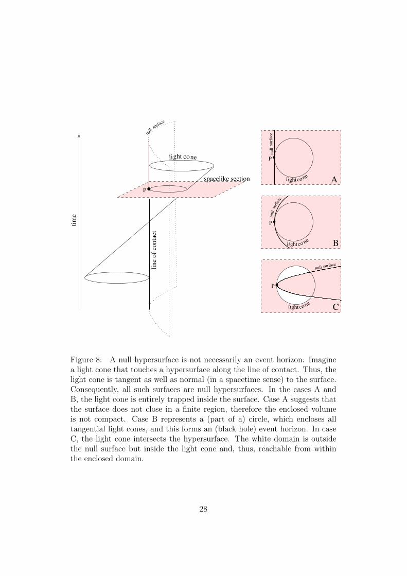
In 1958, Finkelstein[59] characterized the surface r = 2m as a “semi-permeablemembrane” in spacetime, that is, a surface which can be crossed only in onedirection. As soon as our boat has passed the event horizon, it can nevercome back. This property can be formulated in an invariant way: The lightcones at each point of the surface have to nestle tangentially to the mem-brane. In 1964, Penrose[149] termed the null cone which divides observablefrom unobservable regions an event horizon. Mathematically speaking, theevent horizon is characterized by having tangent vectors which are light-likeor null at all points. Therefore, the event horizon is a null hypersurface. Thisis what is meant by a trapped surface[29], see Fig. 8 and Fig. 9, left image: acompact, spacelike, 2-dimensional submanifold with the property that out-going future-directed light rays converge in both directions everywhere onthe submanifold. All these characterizations quite intuitively show up in thePenrose-Kruskal diagram to be discussed later.

In view of the preceding paragraph, we define a black hole as a regionof spacetime separated from infinity by an event horizon, see Carroll[29] andBrill[22].

Observational evidence in favor of black holes was reviewed by Narayanand McClintock[129].

Killing horizon

The stationary limit surface is rendered more precise in the notion of a Killinghorizon. A particle at rest (with respect to the infinity of an asymptoticallyflat, stationary spacetime) is to be required to follow the trajectories of thetimelike Killing vector9. However, if we have a Killing vector K describing

9 Using the definitions of the covariant derivative and of the Christoffel symbols, wecan derive the following equation for an arbitrary vector K,

Kα∂α gµν = 2∇(µKν) − 2gα(µ∂ν)Kα . (39)

Assuming Kα and gµν to be constant in time, demands ∇(µKν) = 0. Hence K has to bea Killing vector. In this coordinate system, we have KαKα = g00. Although K acts astime translation, it is not necessarily timelike!

26

a stationary spacetime, then at some points K may become lightlike, thatis KµKµ = 0. If all these points build up a hypersurface Σ, then this nullhypersurface is called a Killing horizon. Apparently, this notion is of a localcharacter, in contrast to the definition of an event horizon, the definition ofwhich refers to events in the future, it is of a nonlocal character, see Fig. 8.

As we will see for the Schwarzschild black hole, see Fig. 9, outside theblack hole the Killing vector is timelike, that is, KµKµ < 0, on the Killinghorizon it becomes null KµKµ = 0 (by definition of the horizon), and insideit becomes spacelike KµKµ > 0.

In the Schwarzschild case it will turn out that the event horizon andKilling horizon coincide, in the Kerr case they separate.

Surface gravity

From the definition of the Killing horizon it can be shown[29] that the quan-tity

κ2 := −1

2(∇µKν)(∇µKν) |Σ (40)

is constant on the Killing horizon and positive. The quantity κ is calledsurface gravity. In simple cases, it has the interpretation of an accelerationor gravitational force per unit mass on the horizon. In the Schwarzschildspacetime it takes the value κ = 1/4m, which is the acceleration of a particlewith unit mass as seen from infinity, compare with the Newtonian “fieldstrength” (2) for r = 2m:

f =GM

r2=

m

(2m)2=

1

4m. (41)

In general, there is no such simple interpretation.

Infinite redshift

Another property associated with the surface KµKν = 0 is the infinite red-shift. In view of the relation for the general relativistic time delay,

τ0(~xB) =

√gtt(~xB)√gtt(~xA)

τ0(~xA) .

gtt → 0 can be interpreted as follows. Consider τ0(~xB) the time measured bya clock B resting well away from the Killing horizon, whereas clock A withτ0(~xA) is nearly at the Killing horizon. If gtt(~xA) → 0 we get τ0(~xB) → ∞.From the point of view of clock B, clock A’s last signal, right before A hits

27

li ght neco

li ght neco

li ght neco

ght coneli li

ne

of

con

tact

spacelike section

P

P

P

P

nu

llsu

rfac

esu

rfac

e

null

surfacenull

surface

null

A

B

C

tim

e

Figure 8: A null hypersurface is not necessarily an event horizon: Imaginea light cone that touches a hypersurface along the line of contact. Thus, thelight cone is tangent as well as normal (in a spacetime sense) to the surface.Consequently, all such surfaces are null hypersurfaces. In the cases A andB, the light cone is entirely trapped inside the surface. Case A suggests thatthe surface does not close in a finite region, therefore the enclosed volumeis not compact. Case B represents a (part of a) circle, which encloses alltangential light cones, and this forms an (black hole) event horizon. In caseC, the light cone intersects the hypersurface. The white domain is outsidethe null surface but inside the light cone and, thus, reachable from withinthe enclosed domain.

28

the Killing horizon, will not reach B in a finite time, that is, never. To put ita little bit different: Signals sent with respect to A with constant frequencyarrive increasingly delayed at B; for B the frequency approaches zero. Thisis called infinite redshift.

Let us work out these ideas for the Schwarzschild solution and let us take“photons” in spacetime instead of boats on a lake.

2.5 Using light rays as coordinate lines

Schwarzschild coordinates exhibit a coordinate singularity at r = 2m. Thisobstructs the discussion of the event horizon considerably. As we have seen,light rays penetrate the horizon without difficulty. This suggests to use lightrays as coordinate lines. Therefore we introduce in- and outgoing Eddington-Finkelstein coordinates. By combining both, we arrive at Kruskal-Szekerescoordinates, which provide a regular coordinate system for the whole Schwarz-schild spacetime.

Eddington-Finkelstein coordinates

In relativity, light rays, the quasi-classical trajectories of photons, are nullgeodesics. In special relativity, this is quite obvious, since in Minkowski spacethe geodesics are straight lines and “null” just means v = c. A more rigorousargument involves the solution of the Maxwell equations for the vacuumand the subsequent determination of the normals to the wave surface (rays)which turn out to be null geodesics. This remains valid in general relativity.Null geodesics can be easily obtained by integrating the equation 0 = ds.We find for the Schwarzschild metric, specializing to radial light rays withdφ = 0 = dθ,

t = ±(r + 2m ln

∣∣∣ r2m− 1∣∣∣)+ const . (42)

If we denote with r0 the solution of the equation r + 2m ln∣∣ r

2m− 1∣∣ = 0, we

have for the t-coordinate of the light ray t(r0) =: v. Hence, if r = r0, we canuse v to label light rays. In view of this, we introduce v and u

v := t+ r + 2m ln∣∣∣ r2m− 1∣∣∣ , (43)

u := t− r − 2m ln∣∣∣ r2m− 1∣∣∣ . (44)

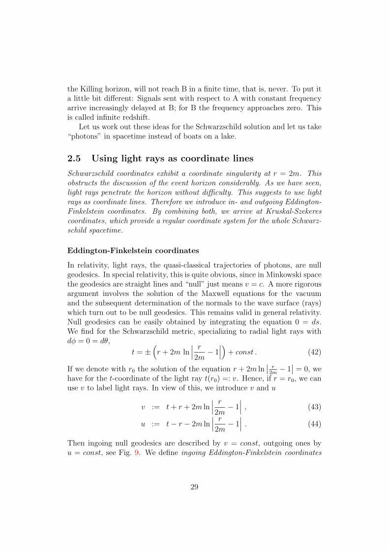
Then ingoing null geodesics are described by v = const, outgoing ones byu = const, see Fig. 9. We define ingoing Eddington-Finkelstein coordinates

29

r

t’

v

incoming photon

outg

oin

g p

hoto

n

r=2m

u

t’

r

outg

oing

pho

ton

inco

min

g p

hoto

n

r=2m

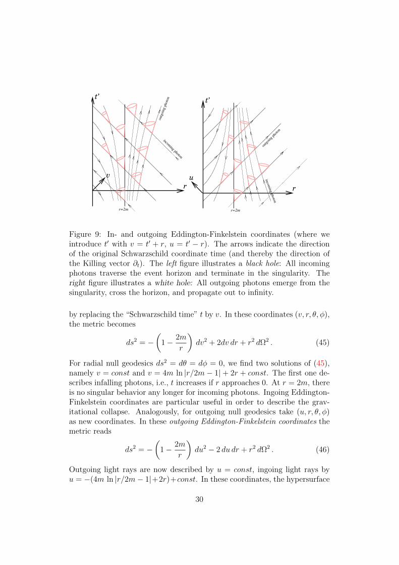
Figure 9: In- and outgoing Eddington-Finkelstein coordinates (where weintroduce t′ with v = t′ + r, u = t′ − r). The arrows indicate the directionof the original Schwarzschild coordinate time (and thereby the direction ofthe Killing vector ∂t). The left figure illustrates a black hole: All incomingphotons traverse the event horizon and terminate in the singularity. Theright figure illustrates a white hole: All outgoing photons emerge from thesingularity, cross the horizon, and propagate out to infinity.

by replacing the “Schwarzschild time” t by v. In these coordinates (v, r, θ, φ),the metric becomes

ds2 = −(

1− 2m

r

)dv2 + 2dv dr + r2 dΩ2 . (45)

For radial null geodesics ds2 = dθ = dφ = 0, we find two solutions of (45),namely v = const and v = 4m ln |r/2m− 1| + 2r + const. The first one de-scribes infalling photons, i.e., t increases if r approaches 0. At r = 2m, thereis no singular behavior any longer for incoming photons. Ingoing Eddington-Finkelstein coordinates are particular useful in order to describe the grav-itational collapse. Analogously, for outgoing null geodesics take (u, r, θ, φ)as new coordinates. In these outgoing Eddington-Finkelstein coordinates themetric reads

ds2 = −(

1− 2m

r

)du2 − 2 du dr + r2 dΩ2 . (46)

Outgoing light rays are now described by u = const, ingoing light rays byu = −(4m ln |r/2m− 1|+2r)+const. In these coordinates, the hypersurface

30

r = 2m (the “horizon”) can be recognized as a null hypersurface (its normalis null or lightlike) and as a semi-permeable membrane.

Kruskal-Szekeres coordinates

Next we try to combine the advantages of in- and outgoing Eddington-Finkelstein coordinates in the hope to obtain a fully regular coordinatesystem of the Schwarzschild spacetime. Therefore we assume coordinates(u, v, θ, φ). Some (computer) algebra yields the corresponding representa-tion of the metric:

ds2 = −(

1− 2m

r(u, v)

)du dv + r2(u, v) dΩ2 . (47)

Unfortunately, we still have a coordinate singularity at r = 2m. We can getrid of it by reparametrizing the surfaces u = const and v = const via

v = exp( v

4m

), u = − exp

(− u

4m

). (48)

In these coordinates, the metric reads (r = r(u, v) is implicitly given by (48)and (44), (43), rS = 2m)

ds2 = − 4r3S

r(u, v)exp

(−r(u, v)

2m

)dv du+ r2(u, v) dΩ2 . (49)

Again, we go back from u and v to time- and space-like coordinates:

t :=1

2(v + u) , r :=

1

2(v − u) . (50)

In terms of the original Schwarzschild coordinates we have

r =

√∣∣∣ r2m− 1∣∣∣ exp

( r

4m

)cosh

t

4m, (51)

t =

√∣∣∣ r2m− 1∣∣∣ exp

( r

4m

)sinh

t

4m. (52)

The Schwarzschild metric

ds2 =4r3

S

rexp

(− r

2m

) (−dt 2 + dr2

)+ r2 dΩ2 , (53)

in these Kruskal-Szekeres coordinates (t, r, θ, φ), behaves regularly at thegravitational radius r = 2m. If we substitute (53) into the Einstein equation

31

(via computer algebra), then we see that it is a solution for all r > 0. Eqs.(51)and (52) yield

r2 − t 2 =∣∣∣ r2m− 1∣∣∣ exp

( r

2m

). (54)

Thus, the transformation is valid only for regions with |r| > t. However, wecan find a set of transformations which cover the entire (t, r)-space. They arevalid in different domains, indicated here by I, II, III, and IV, to be explainedbelow:

(I)

t =

√r

2m− 1 exp

(r

4m

)sinh t

4m

r =√

r2m− 1 exp

(r

4m

)cosh t

4m

(55)

(II)

t =

√1− r

2mexp

(r

4m

)cosh t

4m

r =√

1− r2m

exp(r

4m

)sinh t

4m

(56)

(III)

t = −

√r

2m− 1 exp

(r

4m

)sinh t

4m

r = −√

r2m− 1 exp

(r

4m

)cosh t

4m

(57)

(IV)

t = −

√1− r

2mexp

(r

4m

)cosh t

4m

r = −√

1− r2m

exp(r

4m

)sinh t

4m

(58)

The inverse transformation is given by( r

2m− 1)

exp( r

2m

)= r2 − t 2 , (59)

t

4m=

Artanh t/r , for (I) and (III) ,

Artanh r/t , for (II) and (IV) .. (60)

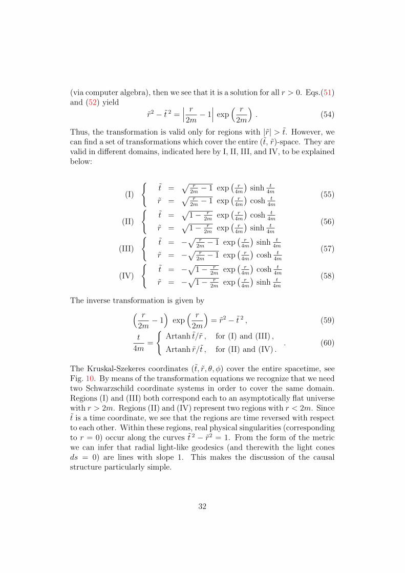
The Kruskal-Szekeres coordinates (t, r, θ, φ) cover the entire spacetime, seeFig. 10. By means of the transformation equations we recognize that we needtwo Schwarzschild coordinate systems in order to cover the same domain.Regions (I) and (III) both correspond each to an asymptotically flat universewith r > 2m. Regions (II) and (IV) represent two regions with r < 2m. Sincet is a time coordinate, we see that the regions are time reversed with respectto each other. Within these regions, real physical singularities (correspondingto r = 0) occur along the curves t 2 − r2 = 1. From the form of the metricwe can infer that radial light-like geodesics (and therewith the light conesds = 0) are lines with slope 1. This makes the discussion of the causalstructure particularly simple.

32

IVt=1.5m

t=-4m

t=4m

r=3.4m

r=4m

IIII

r=2.5m

t=-1.5mII

t

r

t

~

~

r

IIIIV

r=2

m

r=1.3m

r=1.8m

light cone

ingoing

t=-4m

t=1.5m

t=-1.5m

t=-4m

-r

outg

oing

-t~

~

t

r

r=2

m

II I

r=0

r=0

r=2m

Figure 10: Kruskal-Szekeres diagram of the Schwarzschild spacetime.

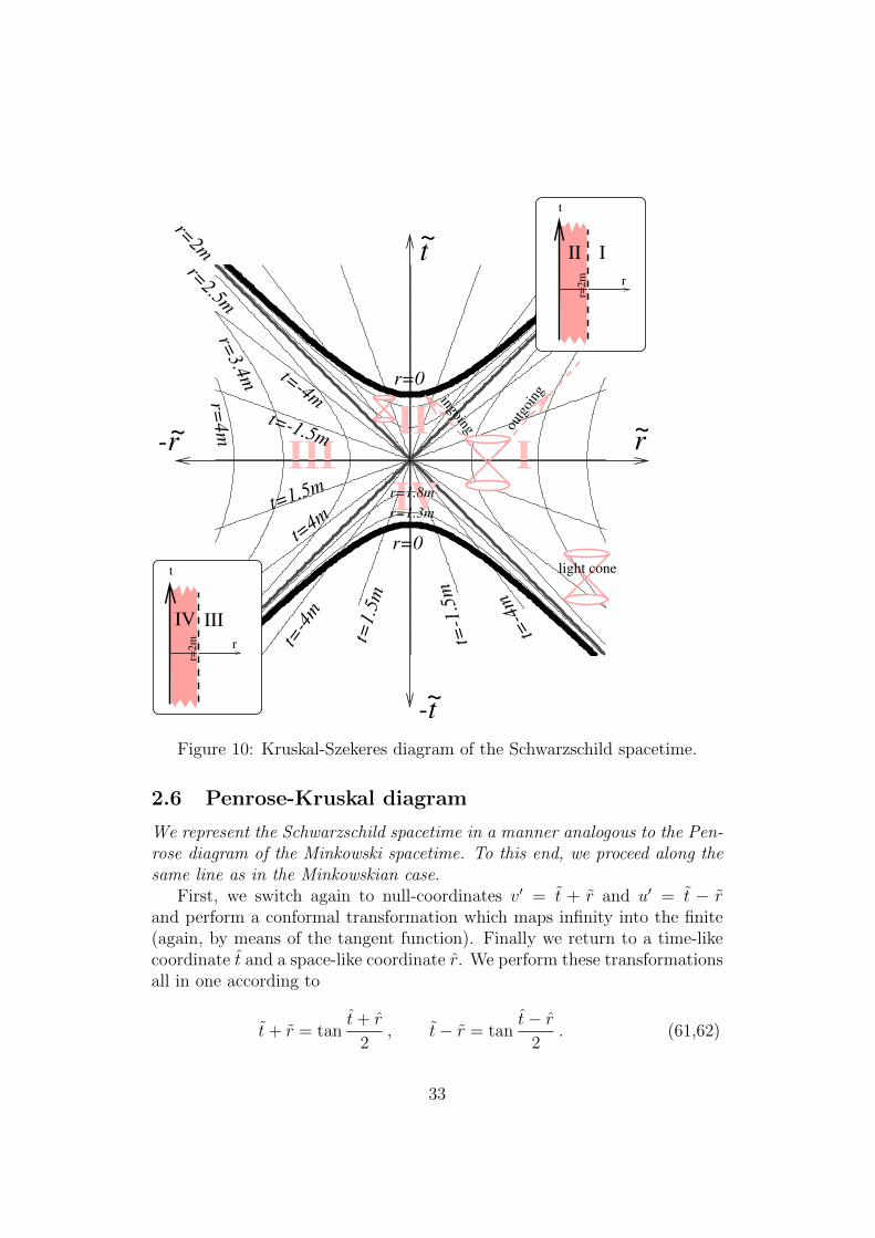
2.6 Penrose-Kruskal diagram

We represent the Schwarzschild spacetime in a manner analogous to the Pen-rose diagram of the Minkowski spacetime. To this end, we proceed along thesame line as in the Minkowskian case.

First, we switch again to null-coordinates v′ = t + r and u′ = t − rand perform a conformal transformation which maps infinity into the finite(again, by means of the tangent function). Finally we return to a time-likecoordinate t and a space-like coordinate r. We perform these transformationsall in one according to

t+ r = tant+ r

2, t− r = tan

t− r2

. (61,62)

33

II

IV

III II0−π

I0π

I+I+

I−I−

singularity r = 0

singularity r = 0

r=

2mI+ I+

I− I−

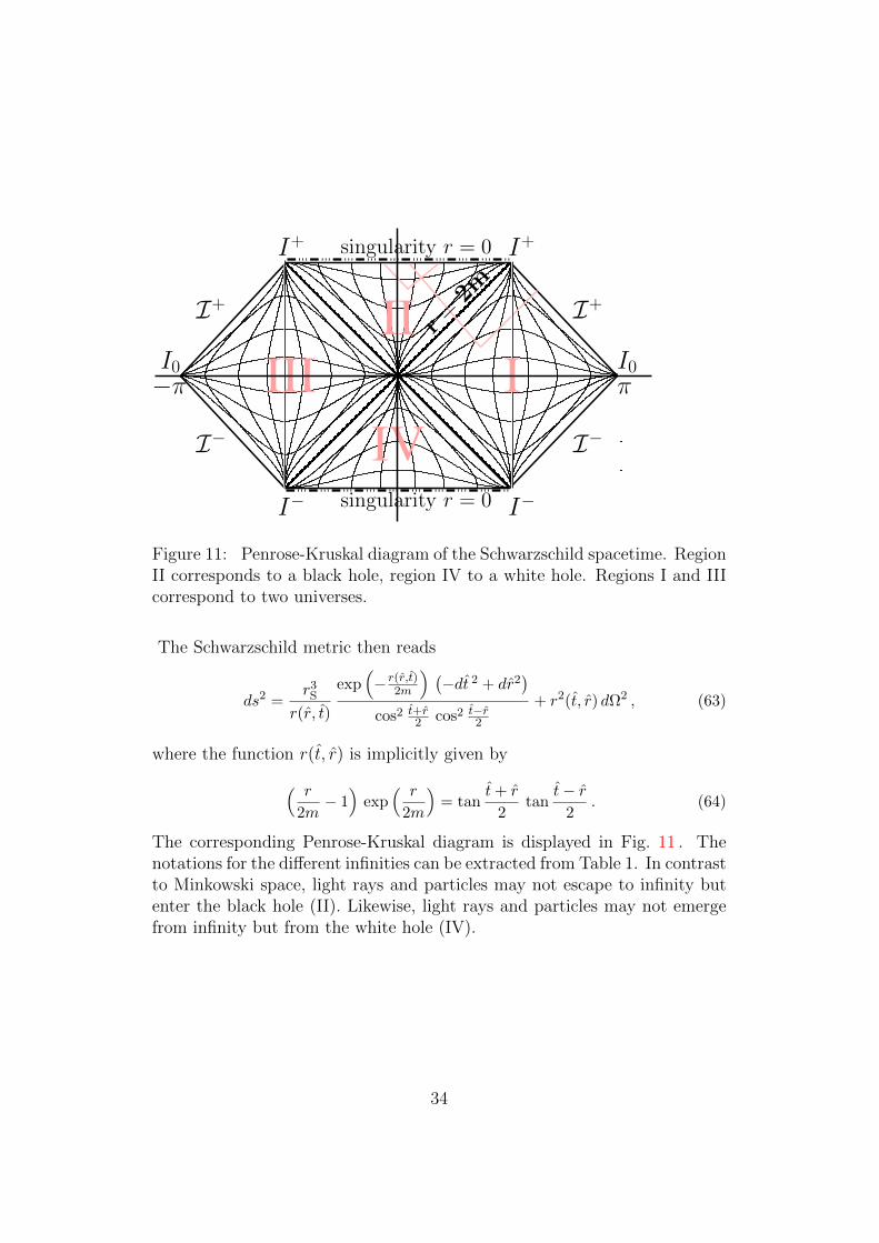
Figure 11: Penrose-Kruskal diagram of the Schwarzschild spacetime. RegionII corresponds to a black hole, region IV to a white hole. Regions I and IIIcorrespond to two universes.

The Schwarzschild metric then reads

ds2 =r3

S

r(r, t)

exp(− r(r,t)

2m

) (−dt 2 + dr2

)cos2 t+r

2 cos2 t−r2

+ r2(t, r) dΩ2 , (63)

where the function r(t, r) is implicitly given by( r

2m− 1)

exp( r

2m

)= tan

t+ r

2tan

t− r2

. (64)

The corresponding Penrose-Kruskal diagram is displayed in Fig. 11 . Thenotations for the different infinities can be extracted from Table 1. In contrastto Minkowski space, light rays and particles may not escape to infinity butenter the black hole (II). Likewise, light rays and particles may not emergefrom infinity but from the white hole (IV).

34

2.7 Adding electric charge and the cosmological con-stant: Reissner Nordstrom

As mentioned in the historical remarks, soon after Schwarzschild’s solution,the first generalizations, including electric charge and the cosmological con-stant were published. We can be even quicker . . . We already calculated theRicci tensor for the Gullstrand-Painleve ansatz. If we use the well-knownenergy-momentum tensor for a point charge[81], the field equation may bewritten as10

Rµν − 1

2Rδνµ + Λ δνµ = κλ0

q2

2r4diag(−1,−1, 1, 1) . (65)

Taking the trace, we find R = 4Λ and arrive at

R22 = R3

3 =2∂r(rψ)

r2= Λ− q2

r4. (66)

This equation can be integrated elementarily,

2ψ =1

3Λr2 − q2

r2+

2α

r. (67)

This function also solves the remaining two field equations. The integrationconstant α is again the mass m. Substituted into (37) and transformed toSchwarzschild coordinates (f = 1− 2ψ) the solution reads

ds2 = −f(r) dt2 +dr2

f(r)+ r2 dΩ2 , (68)

with

f(r) := 1− 2m

r+q2

r2− Λ

3r2 . (69)

A detailed derivation using Schwarzschild coordinates and computer algebracan be found in Puntigam et al.[158]

A discussion of the Reissner-Nordstrom(-de Sitter) solution can be foundin Griffiths & Podolsky[69], for example. We only remark, that we recoverthe Schwarzschild solution for q = 0 and Λ = 0. The algebraic structure ofthe solution is identical to the Schwarzschild case. Thus, we find, in general,a singularity at r = 0. However, a pure cosmological solution, m = 0, q = 0

10Einstein’s gravitational constant is denoted by κ, λ0 =√

ε0µ0

is the admittance of the

vacuum. With c = 1 and G = 1 we have κλ0 = 2.

35

and Λ 6= 0, possesses no singularity and no horizon! On the other hand, anelectrically charged black hole, Λ = 0, exhibits two horizons,

f(r) = 0 ⇔ r± = m±√m2 − q2 . (70)

In this respect, the charged black hole shows some similarities to a rotating(Kerr) black hole. We will pick up this discussion in Sec.3.4.

2.8 The interior Schwarzschild solution and the TOVequation

In the last section we investigated the gravitational field outside a sphericallysymmetric mass-distribution. Now it is time to have a look inside matter,see Adler, Bazin, and Schiffer [1]. Of course, in a first attempt, we haveto make decisive simplifications on the internal structure of a star. We willconsider cold catalyzed stellar material during the later phase of its evolutionwhich can be reasonably approximated by a perfect fluid. The typical massdensities are in the range of ≈ 107 g/cm3 (white dwarfs) or ≈ 1014 g/cm3

(neutron stars, e.g., pulsars). In this context we assume vanishing angularmomentum.

We start again from a static and spherically symmetric metric

ds2 = −eA(r) c2 dt2 + eB(r) dr2 + r2 dΩ2 (71)

and the energy-momentum tensor

Tµν =(ρ+

p

c2

)uµ uν + p gµν , (72)

where ρ = ρ(r) is the spherically symmetric mass density and p = p(r) thepressure (isotropic stress). This has to be supplemented by the equation ofstate which, for a simple fluid, has the form p = p(ρ).

We compute the non-vanishing components of the field equation by meansof computer algebra as (here κ = 8πG/c4 is Einstein’s gravitational constantand ()′ = d/dr)

− eBκr2c2ρ+ eB +B′r − 1 = 0 , (73)

−eBκpr2 − eB + A′r + 1 = 0 , (74)

−4eBκpr + 2A′′r + (A′)2r − A′B′r + 2A′ − 2B′ = 0 . (75)

The (φ, φ)-component turns out to be equivalent to the (θ, θ)-component.For convenience, we define a mass function m(r) according to

e−B =: 1− 2m(r)

r. (76)

36

We can differentiate (76) with respect to r and find, after substituting(73), a differential equation for m(r) which can be integrated, provided ρ(r)is assumed to be known

m(r) =

∫ r

0

κ

2ρc2 ξ2 dξ . (77)

Differentiating (74) and using all three components of the field equation, weobtain a differential equation for A:

A′ = − 2p′

p+ ρc2. (78)

We can derive an alternative representation of A′ by substituting (76) into(74). Then, together with (78), we arrive at the Tolman-Oppenheimer-Volkoff(TOV) equation

p′ = −(ρc2 + p)(m + κ pr3/2)

r(r− 2m). (79)

Terms that survive in the Newtonian limit are emphasized by boldface letters.The system of equations consisting of (77), (78), the TOV equation (79),and the equation of state p = p(ρ) forms a complete set of equations for theunknown functions A(r), ρ(r), p(r), and m(r), with

ds2 = −eA(r) c2 dt2 +dr2

1− 2m(r)r

+ r2 dΩ2 . (80)

These differential equations have to be supplemented by initial conditions.In the center of the star, there is, of course, no enclosed mass. Hence we

demand m(0) = 0. The density has to be finite at the origin, i.e. ρ(0) = ρc,where ρc is the density of the central region. At the surface of the star,at r = R, we have to match matter with vacuum. In vacuum, there isno pressure which requires p(R) = 0. Moreover, the mass function shouldthen yield the total mass of the star, m(R) := GM/c

2. Finally, we haveto match the components of the metric. Therefore, we have to demandexp[A(r0)] = 1− 2m(R)/R.

Equations (73), (74), (75) and certain regularity conditions which gener-alize our boundary conditions, that is,

• regularity of the geometry at the origin,

• finiteness of central pressure and density,

• positivity of central pressure and density,

37

• positivity of pressure and density,

• monotonic decrease of pressure and density,

impose conditions on the functions ρ and p. Then, even without the explicitknowledge of the equation of state, the general form of the metric can bedetermined. For recent work, see Rahman and Visser [162] and the literaturegiven there.

We can obtain a simple solution, if we assume a constant mass density

ρ = ρ(r) = const. (81)

One should mention here that ρ is not the physically observable fluid density,which results from an appropriate projection of the energy-momentum tensorinto the reference frame of an observer. Thus, this model is not as unphysicalas it may look at the first. However, there are serious but more subtleobjections which we will not discuss further in this context.

When ρ = const., we can explicitly write down the mass function (77),

m(r) =r3

2R2, with R =

√3

κρc2, m :=

R3

2R2. (82)

This allows immediately to determine one metric function

eB =1

1− r2

R2

. (83)

The TOV equation (79) factorizes according to

dp

dr= −1

2(ρc2 + p)(1 + κR2p)

r

R2 − r2. (84)

It can be elementarily solved by separation of variables,

p(r) = ρc2

√R2 −R2

−√R2 − r2√

R2 − r2 − 3√R2 −R2

. (85)

Using (78) as A′ = −2 [ln(p+ ρc2)]′

and continuous matching to the exte-rior, eventually yields the interior & exterior Schwarzschild solution for aspherically symmetric body [173]

ds2 =

−(

32

√1− R2

R2− 1

2

√1− r2

R2

)2

c2 dt2 + 1

1− r2

R2

dr2 + r2dΩ2 , r ≤ R ,

−(1− 2m

r

)c2 dt2 + 1

1− 2mr

dr2 + r2 dΩ2 , r > R .

(86)

38

The solution is only defined for R < R. For the Sun11 we have M ≈2 × 1030 kg, R ≈ 7 × 108 m and accordingly ρ ≈ 1.4 × 103 kg/m3. This

leads to R ≈ 3 × 1011 m, that is, the radius of the star R is much smallerthan R: R < R. Hence the square roots in (86) remain real.

The condition R < R suggests that a sufficiently massive object cannotbe stable since no static gravitational field seems possible. This conjecturecan be further supported. Even before reaching R, the central pressure be-comes infinite,

p(0) → ∞ for R →√

8

9R , or m →

4

9R . (87)

If there is no static solution and the situation remains spherically symmetric,we are forced to the conclusion that such a mass distribution must radiallycollapse; either in an infinite time or to a single point in space. With reason-able simplifications, it was first shown by Oppenheimer and Snyder[145] thatthe second alternative is true: A very massive object collapses to a blackhole. As various singularity theorems show today, this behavior is indeedgeneric, see Chrusciel et al.[38] and Sec.3.10.

11To ascertain the consistency of dimensions and units, we recollect the basic definitions:

[G] =(m/s)4

N=

m3

kg s2, κ =

8πG

c4.

The mass M carries the unit kg, the mass parameter has the dimension of a length:

m :=GM

c2, [m] =

m3 kg s2

kg s2 m2= m .

The definition of m(r) in Eq.(77) is consistent. For ρ = const, we have

m(r) =κ

2ρc2

1

3r3 =

G

c24

3π r3 ρ =

GM(r)

c2.

Here ρ denotes the physical mass density, [ρ] = kg/m3. Thus

M(r) :=4

3π r3 ρ

is the physical mass with the unit kg.

39

3 The Kerr metric (1963)

After some historical reminiscences (Sec.3.1), we point out how one can ar-rive at the Kerr metric (Sec.3.2). For that purpose, we derive, in cylindricalcoordinates, the four corresponding partial differential equations and explainhow this procedure leads to the Kerr metric. In Sec.3.3, we display the Kerrmetric in three classical coordinate systems. Thereafter we develop the con-cept of the Kerr black hole (Sec.3.4). In Secs.3.5 to 3.7, we depict and dis-cuss the geometrical/kinematical properties of the Kerr metric. Subsequently,in Sec.3.8, we turn to the multipole moments of the mass and the angularmomentum of the Kerr metric, stressing analogies to electromagnetism. InSec.3.9, we present the Kerr-Newman solution with electric charge. Even-tually, in Sec.3.10, we wonder in which sense the Kerr black hole is distin-guished from the other stationary axially symmetric vacuum spacetimes, and,in Sec.3.11, we mention the rotating disk metric of Neugebauer-Meinel as arelevant interior solution with matter.

....When I turned to Alfred Schild, who was still sitting inthe armchair smoking away, and said “Its rotating!” he waseven more excited than I was. I do not remember how wecelebrated, but celebrate we did!

Roy P. Kerr (2009)

3.1 Historical remarks

The search for axially symmetric solutions of the Einstein equation startedin 1917 with static and was extended in 1924 to stationary metrics. It cul-minated in 1963 with the discovery of the Kerr metric.

The Schwarzschild solution, as we have seen, describes the gravitationalfield of a spherically symmetric body. Obviously, most planets, moons, andstars rotate so that spherical symmetry is lost and one spatial direction isdistinguished by the 3-dimensional angular momentum vector J of the body.Hence the next problem to attack was to search for the gravitational field ofa massive rotating body.

When one considers a static and axially symmetric situation—this is thecase if the body does not carry angular momentum—then one can choose therotation axis as the z-axis of a cylindrical polar coordinate system: x1 = z,x2 = ρ and x3 = φ. Then static axial symmetry means that the componentsof the metric gµν = gµν(z, ρ) do not depend on the time t and the azimuthal

40

angle φ (we have here one timelike and one spacelike Killing vector12).Already in 1917, Weyl[188] started to investigate static axially symmetric

vacuum solutions of Einstein’s field equation. He took cylindrical coordinatesand proposed the following “canonical” form of the static axisymmetric vac-uum line element:13

ds2 = fdt2 −h(dz2 + dρ2) +

ρ2dφ2

f

; (89)

here f = f(z, ρ) and h = h(z, ρ) and (x0 = t, x1 = z, x2 = ρ, x3 = φ).Weyl was led, in analogy to Newton’s theory, to a Poisson equation andfound thereby a family of static cylindrically symmetric solutions that couldbe understood as the exterior field of a line distribution of mass along therotation axis. Similar investigations were undertaken by Levi-Civita[108](1917/19).

In the year 1918, Lense and Thirring[107] investigated a rotating body.They specified the energy-momentum tensor of a slowly rotating ball of mat-ter of homogeneous density and integrated the Einstein equation in lowestapproximation. They found, for a ball rotating around the z-axis of a spa-tial Cartesian coordinate system, the linearized Schwarzschild solution inisotropic coordinates, see Table 2, together with two new “gravitomagnetic”correction terms in off-diagonal components of the metric (κ is Einstein’sgravitational constant):

ds2 =

(1− 2κM

r

)dt2 −

(1 +

2κM

r

)(dx2 + dy2 + dz2)︸ ︷︷ ︸

linearized Schwarzschild

− 4κJzr3

(xdy − ydx)dt︸ ︷︷ ︸gravitomagnetic term

;

(90)

12Remark on Killing vectors: Consider a point P of spacetime with coordinates xα.We specify a direction ξµ at P . If we have a flat Minkowski space, the components gµνof the metric, given in Cartesian coordinates, would not change under a motion in theξ-direction. However, in a curved spacetime, the gµν will change in general. If ξµ fulfillsthe Killing equations (see Stephani [179])

∇µξν +∇νξµ = 0 , (88)

with ∇ as covariant derivative operator, then ξµ is called a Killing vector, and this vectorspecifies a direction under which the metric does not change. The Schwarzschild metric isstatic, that is, it has one timelike Killing vector along the time coordinate. Furthermore,it is spherically symmetric and thus has three additional spacelike Killing vectors. Inthe Weyl case, because of the axial symmetry around the z-axis, two of those spacelikeKilling vectors get lost. Left over in the Weyl case are the two Killing vectors, one timelike(1)ξt = ∂t and one spacelike (2)ξφ = ∂φ.

13Weyl used ρ → r , φ → ϑ.

41

this is valid for κM r and κJz r2. This gravitomagnetic effect (“theLense-Thirring effect”) is typical for GR: in Newton’s theory a rotating rigidball has the same gravitational field as a non-rotating one. Gravitomagnetismis alien to Newton’s gravitational theory.

In the meantime, the Lense-Thirring effect has been experimentally con-firmed by the Gravity Probe B experiment, see Everitt et al.[55]. They tooka gyroscope in a satellite falling freely around the (rotating) Earth. The spinaxis of the gyroscope pointed to a fixed guide star. Because of the gravito-magnetic term in (90), the gyroscope executed a (very small) Lense-Thirringprecession.14 This can be understood as an interaction of the spin of thegyroscope with the spin of the Earth (spin-spin interaction). Since the gy-roscope moves along a 4d geodesic of a spacetime curved by the mass of theEarth, an additional geodetic precession occurs that has to be experimen-tally separated from the Lense-Thirring term. The geodetic precession hadalready been derived earlier by de Sitter[43] in 1916.15

In spherical polar coordinates we have ydx−xdy = r2 sin2θ dφ. Thus, thegravitomagnetic cross-term in (90) may be rewritten as (4κJz sin2θ/r) dt dφ.A comparison with (89) shows that the canonical Weyl form of the staticmetric is too narrow for describing rotating bodies.

From 1919 on, there appeared further articles on axisymmetric solutions.Levi-Civita16 (1919) reacted to Weyl’s article, and Bach[8] (1922) pushed theLense-Thirring line element to the second order in the approximation.

Then, in 1924, Lanczos[105] extending the Weyl ansatz, started to inves-tigate stationary17 solutions. He found an exact solution for uniformly ro-tating dust. However, his work was apparently partially overlooked. Later,Akeley[2, 3] (1931), Andress[6] (1930) and, in a more definite form, Lewis[109](1932) generalized the static Weyl metric to a stationary one by taking intoaccount the gravitomagnetic term of Lense-Thirring. Lewis (1932) wrote, incylindrical polar coordinates (x1 ρ , x2 z),

ds2 = fdt2 − (eµdx12 + eνdx2

2 + ldφ2)− 2mdt dφ . (91)

He found some exact solutions, typically for rotating cylinders, but not for

14For related experiments, see Ciufolini et al.[35, 34] and Iorio et al.[89, 92] A recentcomprehensive review was given by Will[189]. A textbook presentation may be found inOhanian & Ruffini[143].

15De Sitter had applied it to the Earth-Moon system conceived as a gyroscope precessingaround the Sun (the rotation of which can be neglected). This effect can nowadays bemeasured by Lunar Laser Ranging, see Will[189].

16See Ref.[108], note 8 with the subtitle “Soluzioni binarie di Weyl”.17Stationary spacetimes are those that admit a time-like Killing vector. Static space-

times are stationary spacetimes for which this Killing vector is hypersurface orthogonal;physically this implies time reversal invariance and thus the absence of rotation.

42

rotating balls. It became definitely clear that, in the axially symmetriccase, we may have many different exact vacuum solutions, in contrast tothe case of spherical symmetry with, according to the Birkhoff theorem, theSchwarzschild solution as being unique.

Not much later, van Stockum[184] (1937) determined the gravitationalfield of an infinite rotating cylinder of dust particles, thereby recovering theLanczos solution, inter alia. He fitted one of the interior matter solutions ofLewis to an exterior vacuum solution. Continuing on this line of research,Papapetrou[148] (1953) started from the Andress-Lewis line element, puttingit in a slightly different form, suitable for all stationary axisymmetric vacuumsolutions:

ds2 = −eµ(dρ2 + dz2)− ldφ2 − 2mdφdt+ fdt2 . (92)

The functions µ, l,m, and f depend only on ρ and z. Papapetrou integratedthe field equations and found exact stationary rotating vacuum solutions.However, his solution carried either mass and no angular momentum or an-gular momentum and no mass. Thus[148], “this solution is very special andphysically of little interest.”

A year later, a new result was published, which gave the problem offinding solutions for a rotating ball a new direction. Petrov[152] (1954),from Kazan, classified algebraically the Einstein vacuum field, that is, theWeyl curvature tensor, according to its eigenvalues and eigenvectors. Thisinformation reached the West, in the time of the Cold War, with some delay.A bit later, Pirani[154] (1957) developed a related formalism. It was thePetrov classification and the picking of a suitable class for the gravitationalfield of an isolated body (Petrov class D, with two double principal nulldirections) that finally led to the discovery of the Kerr solution during 1963,ten years after the unphysical solutions of Papapetrou.

Accordingly, it turned out to be a formidable task to find an exact solutionfor a rotating ball and it was only found nearly half a century after thepublication of Einstein’s field equation, namely in 1963 by Roy Kerr [98], aNew Zealander, who worked at the time in Texas within the research group ofAlfred Schild. It is a 2-parameter solution of Einstein’s vacuum field equationwith mass M and rotation (or angular momentum) parameter a := J/M .

The story of the discovery of the Kerr solution was told by Kerr himselfat a conference on the occasion of his 70th birthday [99]. A decisive startingpoint of Kerr’s investigations was, as mentioned, the Petrov classification.Melia, in his popular book[124] “Cracking the Einstein Code”, which doesnot contain any mathematical formula—apart from those appearing in twocopies of Kerr’s notes and on a blackboard in another figure—has told this

43

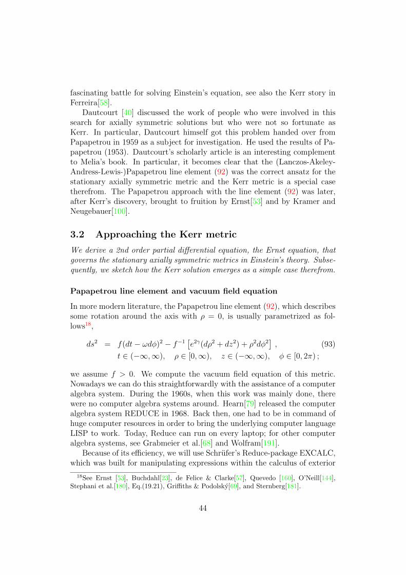
fascinating battle for solving Einstein’s equation, see also the Kerr story inFerreira[58].

Dautcourt [40] discussed the work of people who were involved in thissearch for axially symmetric solutions but who were not so fortunate asKerr. In particular, Dautcourt himself got this problem handed over fromPapapetrou in 1959 as a subject for investigation. He used the results of Pa-papetrou (1953). Dautcourt’s scholarly article is an interesting complementto Melia’s book. In particular, it becomes clear that the (Lanczos-Akeley-Andress-Lewis-)Papapetrou line element (92) was the correct ansatz for thestationary axially symmetric metric and the Kerr metric is a special casetherefrom. The Papapetrou approach with the line element (92) was later,after Kerr’s discovery, brought to fruition by Ernst[53] and by Kramer andNeugebauer[100].

3.2 Approaching the Kerr metric

We derive a 2nd order partial differential equation, the Ernst equation, thatgoverns the stationary axially symmetric metrics in Einstein’s theory. Subse-quently, we sketch how the Kerr solution emerges as a simple case therefrom.

Papapetrou line element and vacuum field equation

In more modern literature, the Papapetrou line element (92), which describessome rotation around the axis with ρ = 0, is usually parametrized as fol-lows18,

ds2 = f(dt− ωdφ)2 − f−1[e2γ(dρ2 + dz2) + ρ2dφ2

], (93)

t ∈ (−∞,∞), ρ ∈ [0,∞), z ∈ (−∞,∞), φ ∈ [0, 2π) ;

we assume f > 0. We compute the vacuum field equation of this metric.Nowadays we can do this straightforwardly with the assistance of a computeralgebra system. During the 1960s, when this work was mainly done, therewere no computer algebra systems around. Hearn[79] released the computeralgebra system REDUCE in 1968. Back then, one had to be in command ofhuge computer resources in order to bring the underlying computer languageLISP to work. Today, Reduce can run on every laptop; for other computeralgebra systems, see Grabmeier et al.[68] and Wolfram[191].

Because of its efficiency, we will use Schrufer’s Reduce-package EXCALC,which was built for manipulating expressions within the calculus of exterior

18See Ernst [53], Buchdahl[23], de Felice & Clarke[57], Quevedo [160], O’Neill[144],Stephani et al.[180], Eq.(19.21), Griffiths & Podolsky[69], and Sternberg[181].

44

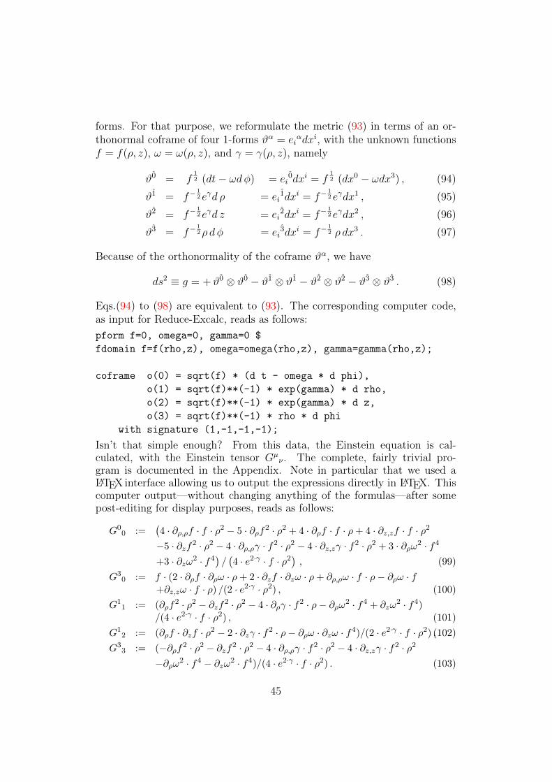
forms. For that purpose, we reformulate the metric (93) in terms of an or-thonormal coframe of four 1-forms ϑα = ei

αdxi, with the unknown functionsf = f(ρ, z), ω = ω(ρ, z), and γ = γ(ρ, z), namely

ϑ0 = f12 (dt− ωdφ) = ei

0dxi = f12 (dx0 − ωdx3) , (94)

ϑ1 = f−12 eγd ρ = ei

1dxi = f−12 eγdx1 , (95)

ϑ2 = f−12 eγd z = ei

2dxi = f−12 eγdx2 , (96)

ϑ3 = f−12ρ d φ = ei

3dxi = f−12 ρ dx3 . (97)

Because of the orthonormality of the coframe ϑα, we have

ds2 ≡ g = +ϑ0 ⊗ ϑ0 − ϑ1 ⊗ ϑ1 − ϑ2 ⊗ ϑ2 − ϑ3 ⊗ ϑ3 . (98)

Eqs.(94) to (98) are equivalent to (93). The corresponding computer code,as input for Reduce-Excalc, reads as follows:

pform f=0, omega=0, gamma=0 $

fdomain f=f(rho,z), omega=omega(rho,z), gamma=gamma(rho,z);

coframe o(0) = sqrt(f) * (d t - omega * d phi),

o(1) = sqrt(f)**(-1) * exp(gamma) * d rho,

o(2) = sqrt(f)**(-1) * exp(gamma) * d z,

o(3) = sqrt(f)**(-1) * rho * d phi

with signature (1,-1,-1,-1);

Isn’t that simple enough? From this data, the Einstein equation is cal-culated, with the Einstein tensor Gµ

ν . The complete, fairly trivial pro-gram is documented in the Appendix. Note in particular that we used aLATEX interface allowing us to output the expressions directly in LATEX. Thiscomputer output—without changing anything of the formulas—after somepost-editing for display purposes, reads as follows:

G00 :=

(4 · ∂ρ,ρf · f · ρ2 − 5 · ∂ρf2 · ρ2 + 4 · ∂ρf · f · ρ+ 4 · ∂z,zf · f · ρ2

−5 · ∂zf2 · ρ2 − 4 · ∂ρ,ργ · f2 · ρ2 − 4 · ∂z,zγ · f2 · ρ2 + 3 · ∂ρω2 · f4

+3 · ∂zω2 · f4)/(4 · e2·γ · f · ρ2

), (99)

G30 := f · (2 · ∂ρf · ∂ρω · ρ+ 2 · ∂zf · ∂zω · ρ+ ∂ρ,ρω · f · ρ− ∂ρω · f

+∂z,zω · f · ρ) /(2 · e2·γ · ρ2) , (100)

G11 := (∂ρf

2 · ρ2 − ∂zf2 · ρ2 − 4 · ∂ργ · f2 · ρ− ∂ρω2 · f4 + ∂zω2 · f4)

/(4 · e2·γ · f · ρ2) , (101)

G12 := (∂ρf · ∂zf · ρ2 − 2 · ∂zγ · f2 · ρ− ∂ρω · ∂zω · f4)/(2 · e2·γ · f · ρ2) ,(102)

G33 := (−∂ρf2 · ρ2 − ∂zf2 · ρ2 − 4 · ∂ρ,ργ · f2 · ρ2 − 4 · ∂z,zγ · f2 · ρ2

−∂ρω2 · f4 − ∂zω2 · f4)/(4 · e2·γ · f · ρ2) . (103)

45

This calculation of the Einstein tensor by machine did not require more thanabout 15 minutes, including the programming and the typing in; for sampleprograms, see Socorro et al.[176] and Stauffer et al.[178].

Inspecting these equations, it becomes immediately clear that the numer-ator of (100) does not depend on γ. In order to get a better overview, weabbreviate the partial derivatives of Reduce ∂ρf by subscripts, fρ, and dropthe superfluous multiplication dots of Reduce. We find

G30 = 0 → 0 = f(ωρρ + ωzz −

1

ρωρ) + 2(fρωρ + fzωz) . (104)

Moreover, by subtracting (103) from (99) we find another equation free of γ:

G00−G3

3 = 0 → 0 = f(fρρ+1

ρfρ+fzz)−f 2

ρ −f 2z +

f 4

ρ2(ω2

ρ+ω2z) . (105)

Left over are the equations (101) and (102), which can be resolved withrespect to the first derivatives of γ:

G11 = 0 → γρ =

ρ

4f 2(f 2ρ − f 2

z ) +f 2

4ρ(ω2

z − ω2ρ) , (106)

G12 = 0 → γz =

ρ

2f 2fρfz −

f 2

2ρωρωz . (107)

Collected, we have these four equations determining the stationary ax-isymmetric vacuum metric:

0 = f(fρρ +1

ρfρ + fzz)− f 2

ρ − f 2z +

f 4

ρ2(ω2

ρ + ω2z) , (108)

0 = f(ωρρ + ωzz −1

ρωρ) + 2(fρωρ + fzωz) , (109)

γρ =ρ

4f 2(f 2ρ − f 2

z ) +f 2

4ρ(ω2

z − ω2ρ) , (110)

γz =ρ

2f 2fρfz −

f 2

2ρωρωz . (111)

Let us underline how effortless—under computer assistance—we arrived atthese four partial differential equations (PDEs) for determining stationaryaxially symmetric solutions of Einstein’s field equation.

Ernst equation (1968)

It is one step ahead, before we arrive at a still more convincing form of thesePDEs. After some attempts, one recognizes that (109) can be written as(

f 2

ρωρ

)ρ

+

(f 2

ρωz

)z

= 0 . (112)

46

With the ansatz (Ω = Ω(ρ, z)),

Ωz =f 2

ρωρ , Ωρ = −f

2

ρωz , (113)

Eq.(112) is identically fulfilled. We substitute (113) into (108):

f(fρρ +1

ρfρ + fzz)− f 2

ρ − f 2z + Ω2

ρ + Ω2z = 0 . (114)

Since (109) is already exploited, we can find Ω by differentiating the Ω’sin (113) with respect to z and ρ, respectively, and by adding the emergentexpressions (ωρz = ωzρ):

f(Ωρρ +1

ρΩρ + Ωzz)− 2fρΩρ − 2fzΩz = 0 . (115)

Eqs.(108) and (115) can be put straightforwardly into a vector analyticalform, if we recall that our functions do not depend on the angle φ:19

f∆f − (∇f) ·∇f + (∇Ω) ·∇Ω = 0 , (116)

f∆Ω− 2(∇f) ·∇Ω = 0 . (117)

The last equation can also be written as ∇ · (f−2∇Ω) = 0. Eqs.(116) and(117) liberate ourselves from the cylindrical coordinates, that is, this expres-sion is now put in form independent of the specific 3d coordinates. With thepotential (i2 = −1)

E := f + iΩ , (118)

which was found by Ernst[53] and Kramer & Neugebauer[100], we find theErnst equation[53]

(Re E) ∆E =∇E · ∇E , (119)

or, in components,

(ReE)

[∂2E∂z2

+1

ρ

∂

∂ρ

(ρ∂E∂ρ

)]=

(∂E∂z

)2

+

(∂E∂ρ

)2

. (120)

The “Re” denotes the real part of a complex quantity. Under stationaryaxial symmetry—the corresponding metric is displayed in (93)—the Ernstequation (119), together with Eqs.(118, 113, 110, 111), are equivalent to thevacuum Einstein field equation.

19In cylindrical coordinates, we have for a vector V and a scalar s the following formulas,

see Jackson[94]:

∇ ·V = 1ρ ∂ρ(ρV1) + ∂zV2 + 1

ρ∂φV3 , ∇2s ≡ ∆s = 1ρ∂ρ(ρ ∂ρs) + ∂2zs+ 1

ρ2 ∂2φs ,

∇s = e1∂ρs+ e2∂zs+ e31ρ∂φs , ∇s ·∇s = (∂ρs)

2 + (∂zs)2 + 1

ρ2 (∂φs)2 .

47

From Ernst back to Kerr

This reduces the problem of axial symmetry to the solution of the secondorder PDE (119). This method, which came along only five years after Kerr’spublication, led to many new exact solutions, amongst them the Kerr solution(1963) as one of the simplest cases. We are only going to sketch how onearrives at the Kerr solution eventually. We follow here closely Buchdahl[23].

One introduces a new complex potential ξ by

E =:ξ − 1

ξ + 1. (121)

Then the Ernst equation becomes

(ξξ − 1)∆ξ = 2ξ∇ξ · ∇ξ , (122)

where the overline denotes complex conjugation. If one has a solution of thisequation, we can determine the functions f , ω and γ by

f = Reξ − 1

ξ + 1, (123)

ωρ = −2ρIm[(ξ + 1)2ξz]

(ξξ − 1)2, ωz = 2ρ

Im[(ξ + 1)2ξρ]

(ξξ − 1)2, (124)

γρ = ρξρξρ − ξzξz(ξξ − 1)2

, γz = 2ρRe(ξρξz)

(ξξ − 1)2. (125)

For rotating bodies, spherical prolate coordinates x, y, with a constant k,are much more adapted:

ρ = k(x2 − 1)12 (1− y2)

12 , z = kxy . (126)

It turns out that one simple potential solving the Ernst equation, with theconstants p and q, is

ξ = px− iqy with p2 + q2 = 1 ; (127)

it leads to the Kerr metric. For this purpose, one has to introduce theredefined constants m := k/p (mass) and a := kq/p (angular momentumper mass) and to execute subsequently the transformations px = (ρ/m)− 1and qy = (a/m) cos θ to the new coordinates ρ and θ. Then one arrives atthe Kerr metric in Boyer-Lindquist coordinates, which is displayed in thetable on the next page. For more detail, compare, for instance, the books ofBuchdahl[23], Islam[93], Heusler[85], Meinel et al.[123], or Griffiths et al.[69].

48

By similar techniques, a Kerr solution with a topological defect was foundby Bergamini et al.[14].

Incidentally, in the context of the Ernst equation, Geroch made the fol-lowing interesting conjecture: A subset of all stationary axially symmetricvacuum space-times, including all of its asymptotically flat members, thatis, in particular the Kerr solution, can be obtained from Minkowski space bytransformations generated by an infinite-dimensional Lie group. This con-jecture was “proved” by Hauser and Ernst[76], see also Ref.[75] However, theproof contained a mistake that was subsequently corrected in Ref.[77]

Starting from 4d ellipsoidal coordinates, Dadhich[39] gave a heuristicderivation of the Kerr metric by requiring, amongst other things, that lightpropagation should be influenced by gravity.

3.3 Three classical representations of the Kerr metric

We collected these three classical versions of the Kerr metric in Table 4, seealso Visser[186].Three more coordinate systems should at least be mentioned:

• Pretorius & Israel[157] double null coordinates:

very convenient to tackle the initial value problem

• Doran[46] coordinates:

Gullstrand-Painleve like; useful in analog gravity

• Debever/Plebanski/Demianski[155] coordinates:

components of the metric are rational polynomials; convenient for (com-puter assisted) calculations

49

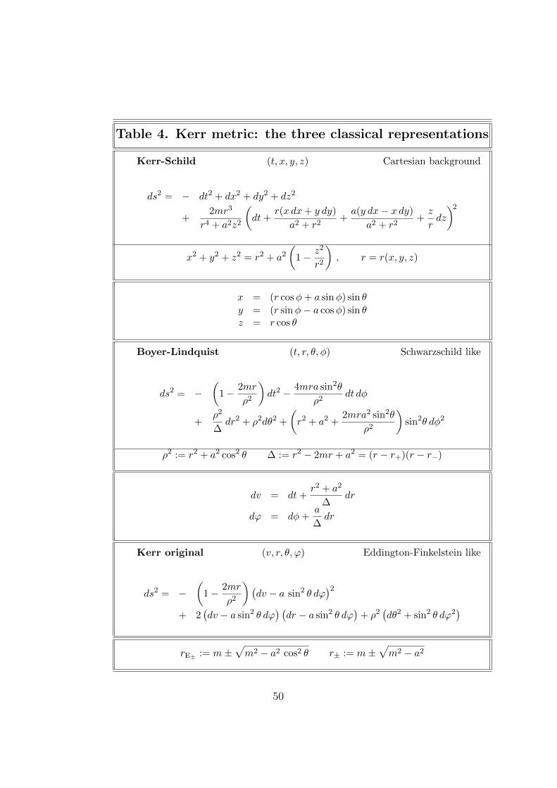
Table 4. Kerr metric: the three classical representations

Kerr-Schild (t, x, y, z) Cartesian background

ds2 = − dt2 + dx2 + dy2 + dz2

+2mr3

r4 + a2z2

(dt+

r(x dx+ y dy)

a2 + r2+a(y dx− x dy)

a2 + r2+z

rdz

)2

x2 + y2 + z2 = r2 + a2

(1− z2

r2

), r = r(x, y, z)

x = (r cosφ+ a sinφ) sin θ

y = (r sinφ− a cosφ) sin θz = r cos θ

Boyer-Lindquist (t, r, θ, φ) Schwarzschild like

ds2 = −(

1− 2mr

ρ2

)dt2 − 4mra sin2θ

ρ2dt dφ

+ρ2

∆dr2 + ρ2dθ2 +

(r2 + a2 +

2mra2 sin2θ

ρ2

)sin2θ dφ2

ρ2 := r2 + a2 cos2 θ ∆ := r2 − 2mr + a2 = (r − r+)(r − r−)

dv = dt+r2 + a2

∆dr

dϕ = dφ+a

∆dr

Kerr original (v, r, θ, ϕ) Eddington-Finkelstein like

ds2 = −(

1− 2mr

ρ2

)(dv − a sin2 θ dϕ

)2+ 2

(dv − a sin2 θ dϕ

) (dr − a sin2 θ dϕ

)+ ρ2

(dθ2 + sin2 θ dϕ2

)rE± := m±

√m2 − a2 cos2 θ r± := m±

√m2 − a2

50

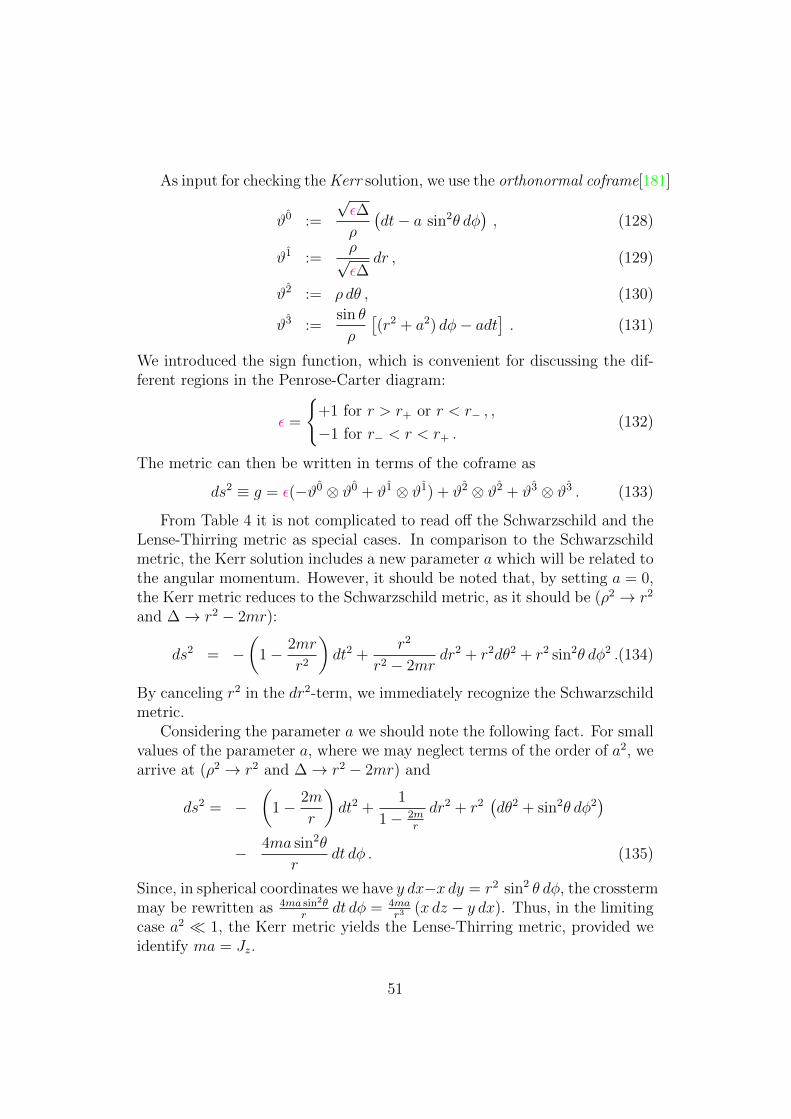
As input for checking the Kerr solution, we use the orthonormal coframe[181]

ϑ0 :=

√ε∆

ρ

(dt− a sin2θ dφ

), (128)

ϑ1 :=ρ√ε∆

dr , (129)

ϑ2 := ρ dθ , (130)

ϑ3 :=sin θ

ρ

[(r2 + a2) dφ− adt

]. (131)

We introduced the sign function, which is convenient for discussing the dif-ferent regions in the Penrose-Carter diagram:

ε =

+1 for r > r+ or r < r− , ,

−1 for r− < r < r+ .(132)

The metric can then be written in terms of the coframe as

ds2 ≡ g = ε(−ϑ0 ⊗ ϑ0 + ϑ1 ⊗ ϑ1) + ϑ2 ⊗ ϑ2 + ϑ3 ⊗ ϑ3 . (133)

From Table 4 it is not complicated to read off the Schwarzschild and theLense-Thirring metric as special cases. In comparison to the Schwarzschildmetric, the Kerr solution includes a new parameter a which will be related tothe angular momentum. However, it should be noted that, by setting a = 0,the Kerr metric reduces to the Schwarzschild metric, as it should be (ρ2 → r2

and ∆→ r2 − 2mr):

ds2 = −(

1− 2mr

r2

)dt2 +

r2

r2 − 2mrdr2 + r2dθ2 + r2 sin2θ dφ2 .(134)

By canceling r2 in the dr2-term, we immediately recognize the Schwarzschildmetric.

Considering the parameter a we should note the following fact. For smallvalues of the parameter a, where we may neglect terms of the order of a2, wearrive at (ρ2 → r2 and ∆→ r2 − 2mr) and

ds2 = −(

1− 2m

r

)dt2 +

1

1− 2mr

dr2 + r2(dθ2 + sin2θ dφ2

)− 4ma sin2θ

rdt dφ . (135)

Since, in spherical coordinates we have y dx−x dy = r2 sin2 θ dφ, the crosstermmay be rewritten as 4ma sin2θ

rdt dφ = 4ma

r3(x dz − y dx). Thus, in the limiting

case a2 1, the Kerr metric yields the Lense-Thirring metric, provided weidentify ma = Jz.

51

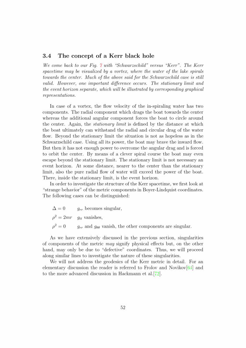
3.4 The concept of a Kerr black hole

We come back to our Fig. 7 with “Schwarzschild” versus “Kerr”. The Kerrspacetime may be visualized by a vortex, where the water of the lake spiralstowards the center. Much of the above said for the Schwarzschild case is stillvalid. However, one important difference occurs. The stationary limit andthe event horizon separate, which will be illustrated by corresponding graphicalrepresentations.

In case of a vortex, the flow velocity of the in-spiraling water has twocomponents. The radial component which drags the boat towards the centerwhereas the additional angular component forces the boat to circle aroundthe center. Again, the stationary limit is defined by the distance at whichthe boat ultimately can withstand the radial and circular drag of the waterflow. Beyond the stationary limit the situation is not as hopeless as in theSchwarzschild case. Using all its power, the boat may brave the inward flow.But then it has not enough power to overcome the angular drag and is forcedto orbit the center. By means of a clever spiral course the boat may evenescape beyond the stationary limit. The stationary limit is not necessary anevent horizon. At some distance, nearer to the center than the stationarylimit, also the pure radial flow of water will exceed the power of the boat.There, inside the stationary limit, is the event horizon.

In order to investigate the structure of the Kerr spacetime, we first look at“strange behavior” of the metric components in Boyer-Lindquist coordinates.The following cases can be distinguished:

∆ = 0 grr becomes singular,

ρ2 = 2mr gtt vanishes,

ρ2 = 0 grr and gθθ vanish, the other components are singular.

As we have extensively discussed in the previous section, singularitiesof components of the metric may signify physical effects but, on the otherhand, may only be due to “defective” coordinates. Thus, we will proceedalong similar lines to investigate the nature of these singularities.

We will not address the geodesics of the Kerr metric in detail. For anelementary discussion the reader is referred to Frolov and Novikov[64] andto the more advanced discussion in Hackmann et al.[72].

52

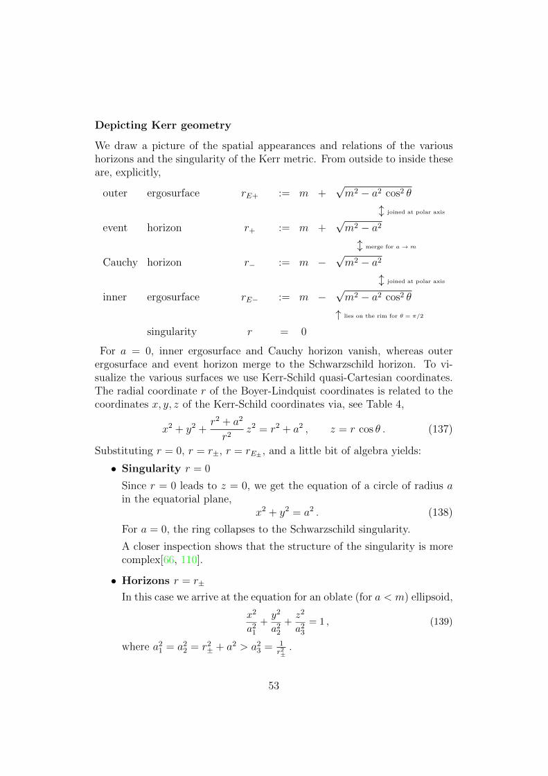
Depicting Kerr geometry

We draw a picture of the spatial appearances and relations of the varioushorizons and the singularity of the Kerr metric. From outside to inside theseare, explicitly,

outer ergosurface rE+ := m +√m2 − a2 cos2 θ

l joined at polar axis

event horizon r+ := m +√m2 − a2

l merge for a→ m

Cauchy horizon r− := m −√m2 − a2

l joined at polar axis

inner ergosurface rE− := m −√m2 − a2 cos2 θ

↑ lies on the rim for θ = π/2

singularity r = 0

For a = 0, inner ergosurface and Cauchy horizon vanish, whereas outerergosurface and event horizon merge to the Schwarzschild horizon. To vi-sualize the various surfaces we use Kerr-Schild quasi-Cartesian coordinates.The radial coordinate r of the Boyer-Lindquist coordinates is related to thecoordinates x, y, z of the Kerr-Schild coordinates via, see Table 4,

x2 + y2 +r2 + a2

r2z2 = r2 + a2 , z = r cos θ . (137)

Substituting r = 0, r = r±, r = rE± , and a little bit of algebra yields:

• Singularity r = 0

Since r = 0 leads to z = 0, we get the equation of a circle of radius ain the equatorial plane,

x2 + y2 = a2 . (138)

For a = 0, the ring collapses to the Schwarzschild singularity.

A closer inspection shows that the structure of the singularity is morecomplex[66, 110].

• Horizons r = r±

In this case we arrive at the equation for an oblate (for a < m) ellipsoid,

x2

a21

+y2

a22

+z2

a23

= 1 , (139)

where a21 = a2

2 = r2± + a2 > a2

3 = 1r2±.

53

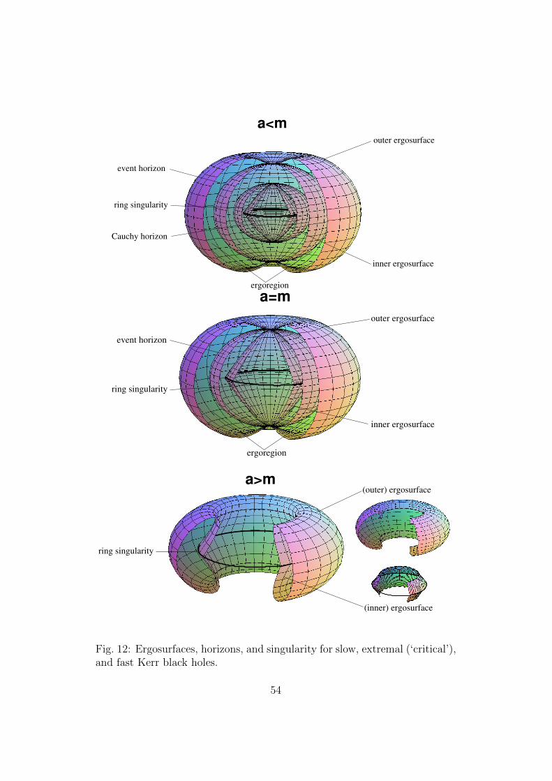
inner ergosurface

outer ergosurface

ergoregion

a<m

Cauchy horizon

event horizon

ring singularity

a=m

ergoregion

event horizon

outer ergosurface

inner ergosurface

ring singularity

a>m(outer) ergosurface

(inner) ergosurface

ring singularity

Fig. 12: Ergosurfaces, horizons, and singularity for slow, extremal (‘critical’),and fast Kerr black holes.

54

• Ergosurfaces r = rE±(θ)

Things are a little bit more involved in this case because r is not con-stant. We can also derive a “ellipsoid-like” equation (for a ≤ m),

x2

a21(θ)

+y2

a22(θ)

+z2

a23(θ)

= 1 , (140)

now with

a21(θ) = a2

2(θ) = r2E±(θ) + a2 , a2

3(θ) =1

r2E±

(θ). (141)

The θ-dependence will deform the ellipsoid. On the equatorial planewith θ = π we have r2

E±= 0. Hence, a1 = a2 = a and a3 diverges. This

results in a non-regular rim on which the ring singularity is located.

For a > m, the rE± is partly not defined, since the term under thesquare-root changes sign, and becomes negative if

cos(θ) =m

a. (142)

This defines two rings with θ1 = arccos(m/a), θ2 = π − θ1 and r = m.As a consequence, the outer ergosurface only extends to these rings fromthe outside, and the inner ergosurface up to the rings from the inside.The outcome is a kind of torus. The center-facing side is constituted bya part of the inner ergosurface (along with the ring singularity), whereasthe outside facing parts are given by a part of the outer ergosurface.

An extensive discussion of the embedding of the ergosurfaces into Eu-clidean space, together with corresponding Mathematica-programs, canbe found in Ref.[114].

The surfaces are visualized in Fig. 12. We did not use a faithful embeddingbut rescaled axes in order to achieve better visibility.

The presence of the term√m2 − a2 requires the distinction of three differ-

ent cases dependent on the values of the mass parameter m and the angularmomentum parameter a:

m > a slow rotation m = a critical rotation m < a fast rotation

The slow rotating case shows the richest structure. Both ergosurfaces andboth horizons are present and distinct from each other. As a approachesm, the event and the Cauchy horizon draw nearer and nearer. At criticalrotation, a = m, both horizons merge into one single event horizon withr = m. Eventually, for fast rotation a > m, the event horizon disappearsand reveals the naked ring singularity which now is located at the inner edgeof the now toroidal shaped (outer) ergosurface.

55

3.5 The ergoregion

We explore the region between the outer ergosurface and the event horizon.There it is not possible to stand still, anything has to rotate, even the eventhorizon. The compulsory rotation in the ergoregion allows one to extractenergy from the black hole. This so-called Penrose process leads to black holethermodynamics.

Constrained rotation

The outer ergosurface, r = RE+ , is defined by the equation g00(rE+) = 0.Thus, it is a surface of infinite redshift and a Killing horizon. For a thirdcharacterization of the ergo surfaces we have to deal not only with radial butalso with rotational motion. Consider the Kerr metric in Boyer-Lindquistcoordinates with dr = dθ = 0,

ds2 = gttdt2 + 2 gtφ dt dφ+ gφφdφ

2 ,

or, after dividing by dt2,(ds

dt

)2

= gtt + 2gtφdφ

dt+ gφφ

(dφ

dt

)2

.

The explicit form of the metric components is not needed here. Note thatΩ = dφ

dtis the angular velocity with respect to a distant observer,(

ds

dt

)2

= gtt + 2gtφ Ω + gφφ Ω2 . (143)

The worldline of a particle has to be timelike, ds2 < 0. Since the last equationis quadratic in Ω, this is only possible between the roots ds2 = 0,

Ωmin/max := − gtφgφφ∓

√(gtφgφφ

)2

− gttgφφ

.

What doesΩmin < Ω < Ωmax

mean?! In flat Minkowski spacetime (with Cartesian coordinates), Ωmin/max =±1 implies that a particle, e.g., may freely circle around a point, restrictedonly by the condition |v| = |r · Ω| < c. In the Kerr spacetime, at r = rE± ,the smallest possible value of Ω becomes 0. The particle may just stay atrest, but can rotate only in one direction, namely in direction of the angular

56

momentum of the black hole. Beyond rE+ , Ω is forced to be larger than zero:The particle must co-rotate with the black hole.

The preceding statement is only correct for radially infalling particles. Ingeneral, the influence of the rotating black hole on the motion of particles ismore complex[165].

Rotation of the event horizon

The behavior of Ω± on the event horizon is quite remarkable. By using theidentities

2mr± = r2± + a2 , ρ2 − r2 = a2 cos2 θ = a2 − a2 sin2 θ , (144)

one finds for the event horizon (r = r+),

Ω+ = Ω− = ΩH :=a

2mr+

. (145)

To interpret this result we use (143) and write

gµν lµ lν |r=r+ = 0 , with lµ = (1, 0, 0,ΩH) . (146)

The integral lines of lµ = xµ,

xµ = (t, r+, θ0,ΩH t) , (147)

define a lightlike hypersurface rotating with a uniform angular velocity: Theevent horizon of a Kerr black hole rotates “rigidly” with ΩH , see in thiscontext Frolov & Frolov[63]. A consequence of this finding is discussed in thenext paragraph.

Penrose process and black hole thermodynamics

The (outer) ergosurface is a Killing horizon, not an event horizon. It ispossible for particles to pass from the inside to the outside. This allows fora peculiar scenario: Since inside the Killing horizon the particle is forced tospin around, it picks up an additional rotational energy. This energy canbe partly extracted by means of the Penrose process. An infalling particletraverses the Killing horizon, picks up rotational energy and subsequentlydecays into two parts. If one part plunges into the event horizon, the otherpart, carrying away some of the rotational energy, can return to the outsideof the Killing horizon. Thus, the region between Killing and event horizonis justly labeled as “ergoregion” (from Greek ergon = work).

57

The observation that energy can also be extracted from the black holegave rise to black hole thermodynamics. The next question is then howthe parameters change if the black hole is infinitesimally disturbed. It wasBekenstein[13] who established a relation between the variations of the mass,the angular momentum, and the area of the event horizon. Using the coframe(185), for λ = 0, we find for the area of the event horizon

A =

∫r = r+t = const.

ϑ2∧ϑ3 =

∫r = r+t = const.

sin θ (r2+a2) dθ∧dφ = 4π(r2

+ + a2). (148)

We can rewrite (148), using (144) and J = ma,

A = 8πmr+ = 8π (m2 −√m4 − J2) . (149)

The differential of this equation is

dA =∂ A

∂mdm+

∂ A

∂JdJ =

8π

κdm− 8π

κΩH dJ , (150)

with

κ =1

2m

√m4 − J2

m2 +√m4 − J2

, ΩH = κJ√

m4 − J2. (151)

The parameter ΩH is the angular velocity of the horizon (145). The param-eter κ is the surface gravity. Eq.(150) can be rewritten as

dm =κ

8πdA+ ΩH dJ . (152)

The infinitesimal change of the mass, dm, is proportional to the the infinites-imal change of the energy, dE. The term ΩH dJ describes the infinitesimalchange of the rotational energy. This suggests the identification of (152)with the first law of thermodynamics. The analogy is still more compellingby observing that, for a given black hole of initial (or irreducible) mass m,the area of the horizon is always increasing. Even by exercising a Penroseprocess, which extracts rotational energy from the black hole, a fragment ofthe incoming particle will fall into the black hole thereby increasing its massand, in turn, the area of the horizon. Accordingly, the area A of the hori-zon behaves formally as if it is proportional to an entropy S and the surfacegravity κ as if it is proportional to a temperature T . In fact, the Hawkingtemperature and the Bekenstein-Hawking entropy turn out to be

T =~

2πkB

κ , S =1

4G~A , (153)

58

with kB as the Boltzmann constant. Eq.(152) together with its thermody-namical interpretation (153) can be considerably generalized thereby estab-lishing the new discipline of “black hole thermodynamics”, see Heusler[85]and Carlip.[28]

3.6 Beyond the horizons

In the Schwarzschild spacetime, event horizon and Killing horizon coincide.In the Kerr spacetime, for m > a, there is an outer Killing horizon, anevent horizon, an inner Killing horizon and an inner horizon. So far, allthe coordinate systems we used for the Kerr metric show singularities at theouter and inner horizons r = r±. The construction of a regular coordinatesystem is possible along the same lines as for the Schwarzschild metric. Ofcourse, the corresponding calculations are much more involved for the Kerrcase. Therefore, we will give more a kind of heuristic approach to motivateKruskal-like coordinates for the Kerr metric.

Using light rays as coordinate lines

Our first task is to construct Eddington-Finkelstein like coordinates for theKerr metric by considering radial light rays. We restrict ourselves to thecase θ = 0 = φ. The Kerr metric in Boyer-Lindquist coordinates reduces to(θ = 0 → ρ2 = r2 + a2 = ∆ + 2mr):

ds2 = −∆

ρ2dt2 +

ρ2

∆dr2 .

Hence, for in-/out-going light rays, ds2 = 0, we find

dt = ±ρ2

∆dr = ± r2 + a2

(r − r+)(r − r−)dr

or, explicitly,

±t =

∫dr

r2 + a2

(r − r−)(r − r+)= r+

r2+ + a2

r+ − r−ln |r − r+|−

r2− + a2

r+ − r−ln |r − r−|+const.

(154)

Unlike in the Schwarzschild spacetime, there form two event horizons, atr = r− and r = r+, respectively. However, as a → 0, r− goes to 0, whereasr+ approaches 2m and the Schwarzschild situation is reproduced.

We next focus on the (Boyer-Lindquist) coordinates (t, r) and how thehorizons etc. will appear in terms of the new coordinates. The other co-ordinates and the regularity of the metric is not addressed. However, all

59

the details can be found in the literature, see Refs.[20, 30, 78]. Using (154)analogously to (42), we introduce Eddington-Finkelstein like coordinates forKerr,

v := t+ r + σ+ ln |r − r+| − σ− ln |r − r−| , (155)

u := t− r − σ+ ln |r − r+|+ σ− ln |r − r−| , (156)

where (according to the notation in Ref.[20])

σ± :=r2± + a2

r+ − r−=

mr±√m2 − a2

. (157)

Again, we can get rid of the coordinate singularity by rescaling u and vanalogously to (48). Since we have two horizons, r = r+ and r = r−, we haveto decide with respect to which singularity we rescale. We firstly choose r+

and define, see (48),

v := exp

(v

2σ+

)=|r − r+|

12

|r − r−|ν2

er+t2σ+ , (158)

u := − exp

(− u

2σ+

)= −|r − r+|

12

|r − r−|ν2

er−t2σ+ , (159)

withν :=

σ−σ+

=r−r+

> 1 . (160)

Again, we go back to time- and space-like coordinates, exactly like in (50),

t :=1

2(v + u) , r :=

1

2(v − u) . (161)

Then we work out the four coordinate patches exactly like (55) to (60).We arrive at a Kruskal like coordinate system. However, there arises animportant difference: The coordinate system still is singular for r = r−. Thiscan be most easily seen from the analog to (59), the inverse transformationto r, which now reads

r2 − t2 = −vu =r − r+

(r − r−)νerσ+ . (162)

The horizon r = r+ is regular in this coordinate system and is described byr = ±t. The transformation(s) are valid in the domain r− < r < +∞

r = r+ : r = ±t as for Schwarzschild

r → +∞ : r2 − t2 → +∞ particularly r → ±∞ for t = 0

r → r− : r2 − t2 → −∞ particularly t→ ±∞ for r = 0

r = rE+ : r2 − t2 = const. > 0 hyperbolas in I, II patches

60

In contrast to the Schwarzschild case, the full upper and lower halfplanesof the (r, t) plane is covered. It is not limited by the hyperbolas of theSchwarzschild singularity r = 0!

We can regularize with respect to r− by introducing

v := − exp

(− v

2σ−

), u := exp

(u

2σ−

). (163)

Now we find

r2 − t2 =r − r−

(r − r+)1ν

e− rσ− . (164)

This coordinate system covers the domain −∞ < r < r+. Like the firstcoordinate system, it contains also the region between the horizons, r− <r < r+. This time, r ≥ r+ is excluded.

r = r− : r = ±t as above

r → −∞ : r2 − t2 →∞ particularly t→ ±∞ for r = 0

r → r+ : r2 − t2 → −∞ particularly r → ±∞ for t = 0

r = rE− : r2 − t2 = const. > 0 hyperbola in I*, II* patches

r = 0 : r2 − t2 = − r−r+< 0 hyperbola in I*, II* patches

Again, the whole (r, t) plane is covered. Note that the spacetime extendsbeyond the ring(!) singularity.

3.7 Penrose-Carter diagram and Cauchy horizon

We compactify the Kruskal-like coordinate system for Kerr, yielding confor-mal Penrose-Carter diagrams. We discuss the analytical extension and therole of the inner horizon as Cauchy horizon.

In order to draw a Penrose-Carter diagram for the Kerr spacetime, wecompactify the coordinates via the tangent function like in Sec.2.6. Theresult looks at first quite similar to Schwarzschild in Fig. 11. However, thecutoff at r = 0 vanishes. The diagrams Fig. 13 and Fig. 14 both show theentire compactified (r, t)-space.

The two coordinate sets overlap in the region between the horizons. Thus,the corresponding coordinate patches have to be identified. And we can evendraw beyond that . . . Patch II is identified with patch IV*, II* with anotherpatch IV**. And so on: We find an infinite sequence of coordinate systems.Formally, this constitutes a maximal analytic extension of the Kerr spacetime.Alas, there are good reasons for not believing in such vast an extension.

The Kerr metric is a vacuum solution of Einstein’s field equation—itdescribes a totally empty spacetime. To render it physically meaningful, we

61

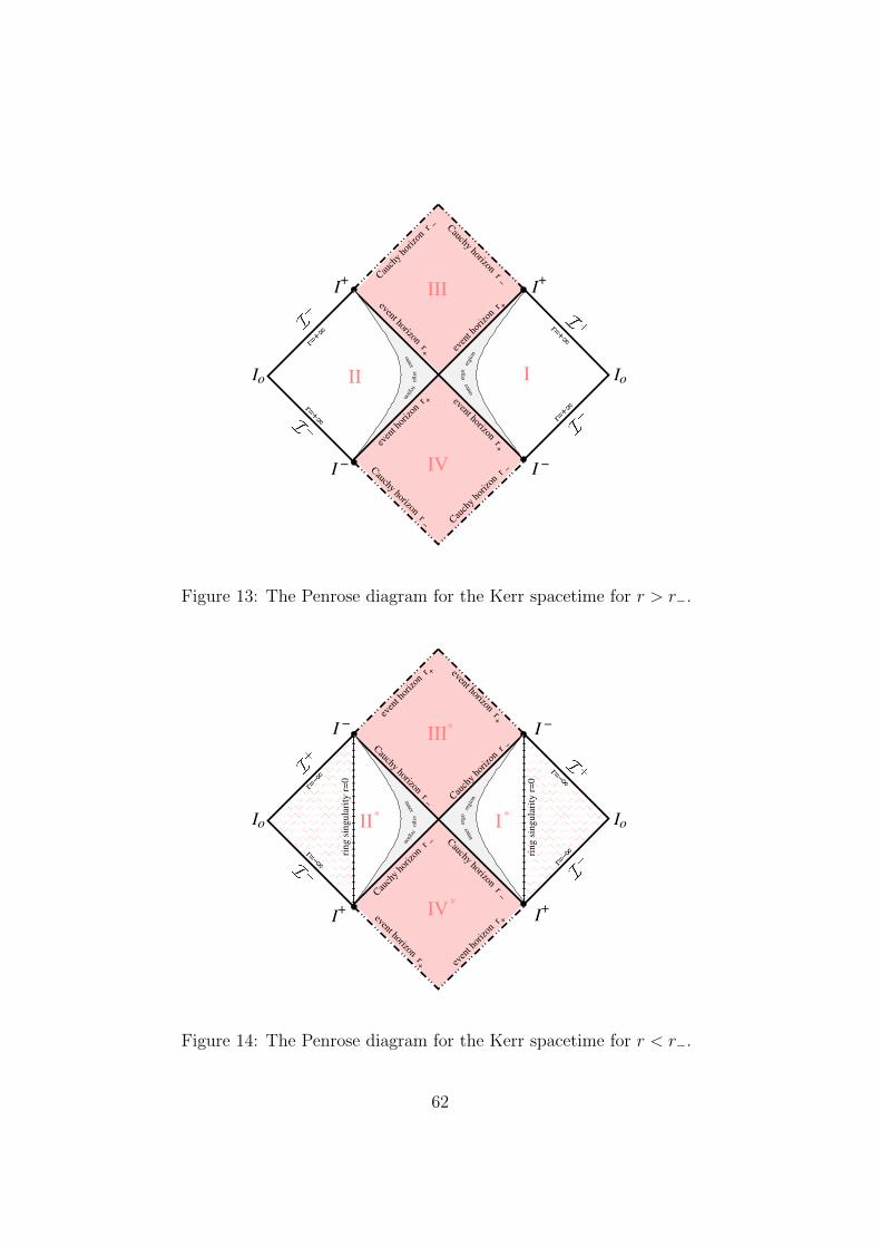
IoIo

I+

I−

I−

I+

III

IV

I

r=+ 8

r=+8r=+ 8

r=+8

even

t hor

izon

r +event horizon r+

even

t hor

izon

r +

Cauchy horizon r

−Cau

chy

horiz

on r

−

event horizon r+

Cau

chy

horiz

on r

−Cauchy horizon r

−

ergo

outerregion

erg

o

oute

rre

gion

II

Figure 13: The Penrose diagram for the Kerr spacetime for r > r−.

ring s

ingula

rity

r=

0

ring s

ingula

rity

r=

0

IoIo

I−

I−

I+

I+

III

IV

event horizon r+

Cau

chy

horiz

on r

−Cauchy horizon r

−

even

t hor

izon

r +

even

t hor

izon

r +event horizon r

+

Cau

chy

horiz

on r

− Cauchy horizon r

−

ergo

region

erg

ore

gioninner

inne

r

* *

r=−8

r=−8

r=− 8

r=− 8

*

*

II I

Figure 14: The Penrose diagram for the Kerr spacetime for r < r−.

62

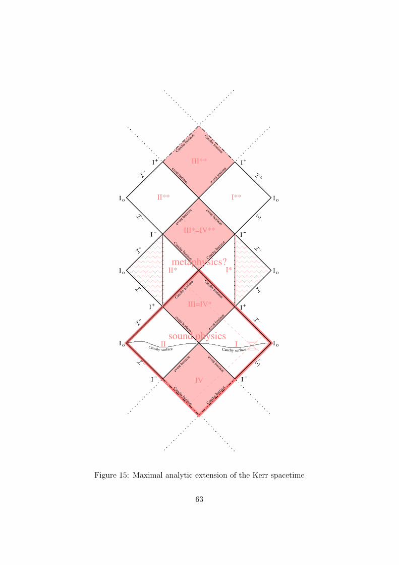
Cauchy surface Cauchy surface

I o

I o

I o

I o

I o

I+

I+

I−I

−

I+

I−

I−

I+

I o III

III=IV*

II** I**

Cau

chy

horiz

on

Cau

chy

horiz

on

Cauchy horizon

Cauchy horizon

Cauchy horizon

Cauchy horizon C

auch

y ho

rizon

Cau

chy

horiz

on

even

t hor

izon

even

t hor

izon

event horizon

event horizon

event horizon even

t hor

izon

event horizon even

t hor

izon

I*

IV

III**

II*

sound physics

metaphysics?

III*=IV**

Figure 15: Maximal analytic extension of the Kerr spacetime

63

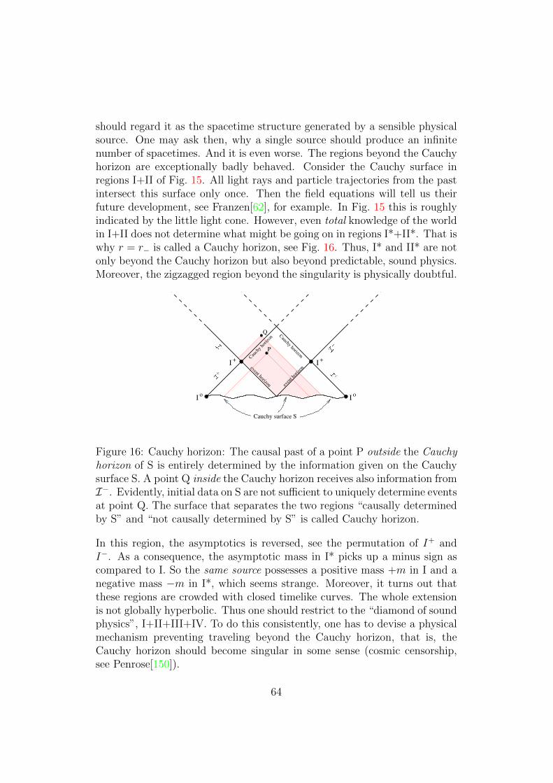
should regard it as the spacetime structure generated by a sensible physicalsource. One may ask then, why a single source should produce an infinitenumber of spacetimes. And it is even worse. The regions beyond the Cauchyhorizon are exceptionally badly behaved. Consider the Cauchy surface inregions I+II of Fig. 15. All light rays and particle trajectories from the pastintersect this surface only once. Then the field equations will tell us theirfuture development, see Franzen[62], for example. In Fig. 15 this is roughlyindicated by the little light cone. However, even total knowledge of the worldin I+II does not determine what might be going on in regions I*+II*. That iswhy r = r− is called a Cauchy horizon, see Fig. 16. Thus, I* and II* are notonly beyond the Cauchy horizon but also beyond predictable, sound physics.Moreover, the zigzagged region beyond the singularity is physically doubtful.

P

Q

Io

Io

I+

I+

event horizon even

t hor

izon

Cau

chy

horiz

onCauchy horizon

Cauchy surface S

Figure 16: Cauchy horizon: The causal past of a point P outside the Cauchyhorizon of S is entirely determined by the information given on the Cauchysurface S. A point Q inside the Cauchy horizon receives also information fromI−. Evidently, initial data on S are not sufficient to uniquely determine eventsat point Q. The surface that separates the two regions “causally determinedby S” and “not causally determined by S” is called Cauchy horizon.

In this region, the asymptotics is reversed, see the permutation of I+ andI−. As a consequence, the asymptotic mass in I* picks up a minus sign ascompared to I. So the same source possesses a positive mass +m in I and anegative mass −m in I*, which seems strange. Moreover, it turns out thatthese regions are crowded with closed timelike curves. The whole extensionis not globally hyperbolic. Thus one should restrict to the “diamond of soundphysics”, I+II+III+IV. To do this consistently, one has to devise a physicalmechanism preventing traveling beyond the Cauchy horizon, that is, theCauchy horizon should become singular in some sense (cosmic censorship,see Penrose[150]).

64

3.8 Gravitoelectromagnetism, multipole moments

The curvature tensor of the Kerr metric is calculated. By squaring it suitably,we find the two quadratic curvature invariants. Subsequently, we determinethe gravitoelectric and the gravitomagnetic multipole moments of the Kerrmetric, and we mention the Simon-Mars tensor the vanishing of which leadsto the Kerr metric.

The analogy between gravity and electrostatics became apparent whenthe Coulomb law was discovered in 1785. The gravitational and the elec-trostatic forces both obeyed an inverse-square law, with the difference thatthe mass can only be positive whereas the electric charge exists with bothsigns. Equal electric charges repel, opposite ones attract; in contrast, gravityis always attractive.

In 1820 electromagnetism was discovered by Oersted, and the emergingunified theory, called “electrodynamics” by Ampere, eventually found itsexpression in the Maxwell equations of 1864. Besides the electric field Erelated to charge, we have the magnetic field B related to moving charge.These fields, together with the electric and magnetic excitations D and H ,respectively, obey the Maxwell equations.

Newton’s gravitational theory was only superseded in 1915/16 by Ein-stein’s gravitational theory, general relativity. However, already in the 1870sphysicists began to speculate whether, besides Newton’s “gravitoelectric”field, related to mass at rest, there may also exist a new “gravitomag-netic” field, accompanying moving mass; for more details and references seeMashhoon[116]. As we saw above, these speculations became a solid basisin general relativity. In (90), the gravitomagnetic Lense-Thirring term sur-faced, which found solid experimental verification in the meantime. Thus, wecan speak with justification of gravitoelectromagnetism[116] (GEM), a notionwhich can guide our intuition, see in this context also Ni and Zimmermann[137].

Gravitoelectromagnetic field strength

Electrodynamics is a linear theory, GR a nonlinear one. Still, if we takea linearized version of GR, there are those strong analogies between elec-trodynamics and gravitodynamics, as worked out, for instance, nicely inRindler’s[165] book. However, the analogies go even further, as pointed outparticularly by Mashhoon[116]. Even in an arbitrary gravitational field, if re-ferred to a Fermi propagated reference frame with coordinates (T,X), GEMis a useful concept. If we apply the geodesic deviation equation (33) to such aframe, the gravitoelectromagnetic field strength, representing the tidal forces,

65

turns out to be[116]20

GEMFαβ = −Rαβ0i(T )X i . (165)

If we develop (33) up to the order linear in the velocity V := dX/dT , wefind

d2X i

dT 2= −R0i0jX

j + 2Rik0jXjV k = −GEMFi0 − 2 GEMFki V

k . (166)

Now we recall that in electrodynamics the electric and the magnetic fieldsE and B, respectively, are accommodated in the 4d electromagnetic fieldstrength tensor according to

(Fαβ) =

0 −E1 −E2 −E3

0 B3 −B2

0 B1

0

= − (Fβα) . (167)

The diamond symbol denotes matrix elements already known because ofthe antisymmetry of the matrix involved. The corresponding 2-form readsF = 1

2Fαβ dx

α ∧ dxβ. Keeping (167) in mind, Eq.(166) can be rewritten as avector equation

d2X

dT 2= −grE− 2V×grB . (168)

In accordance with the equivalence principle, this equation of motion is in-dependent of the mass. The analogy with electromagnetism requires that thegravitoelectric charge, in terms of the mass m, is −1 and the gravitomagneticcharge −2. In electrodynamics, both quantities are +1. The difference comesfrom the vector nature of the electromagnetic potential Aα as compared tothe tensor nature of the gravitational potential gαβ, that is, helicity 1 ascompared to helicity 2. The relation between the gravitomagnetic to thegravitoelectic charge, that is, the gyrogravitomagnetic ratio, is two: grγ = 2.Note that in Gravity Probe-B the authors specify the gyrogravitomagneticratio as 1. However, their gyros carried only orbital angular momentumrather than spin angular momentum. Hence this is to be expected; for moredetailed discussions on this difference, see Ref.[80, 138].

20Alternatively, we could generalize the Newtonian tidal force matrix of (9) to the grav-itoelectric and gravitomagnetic tidal force matrices, Eij = Ri0j0 and Bij = εiklRklj0,respectively, see Scheel & Thorne[169]. Both matrices are symmetric and trace-free. Notethat GEMFαβ is an antisymmetric 4×4 matrix and E and B are both symmetric trace-free3× 3 matrices.

66

It has been pointed out by Ni[139] that the “measurement of the gyrograv-itational ratio of [a] particle would be a further step [138] towards probingthe microscopic origin of gravity. GP-B serves as a starting point for themeasurement of the gyrogravitational factor of particles.”

Quadratic invariants

In electrodynamics, we have two quadratic invariants [81]:

1

2FαβF

αβ = ?(?F ∧ F ) = B2 − E2 ,1

2FαβF

∗αβ = ?(F ∧ F ) = 2E·B ,

(169)where we used for the tensor dual the notation F ∗αβ := 1

2εαβγδFγδ. We also

employed the very concise notation of exterior calculus with the Hodge staroperator.21

The first invariant is proportional to the Maxwell vacuum Lagrangianand is an ordinary scalar, whereas the second one corresponds to a surfaceterm and is a pseudoscalar (negative parity).

Turn now directly to the Kerr metric and list for this example the tidalgravitational forces, which are represented by the curvature tensor. With its20 independent components, it can be represented by a trace-free symmetric6× 6 matrix, see (32). The collective indices A,B, .. = 1, ..., 6 are defined asfollows: tr, tθ, tφ; θφ, φr, rθ −→ 1, 2, 3; 4, 5, 6. We throw the orthonor-mal Kerr coframe (128) to (133) into our computer and out pops the 6 × 6curvature matrix,

(RAB) =

−2E 0 0 2B 0 0 E 0 0 −B 0 E 0 0 −B 2E 0 0 −E 0 −E

= (RBA) , (170)

with

E := mrr2 − 3a2 cos2 θ

(r2 + a2 cos2 θ)3, B := ma cos θ

3r2 − a2 cos2 θ

(r2 + a2 cos2 θ)3. (171)

It is straightforward to identify E as the gravitoelectric and B as the gravit-omagnetic component of the curvature. This is in accordance with (165).

21The Hodge star ?ω of a p-form ω = (1/p!)ωµ1···µpdxµ1∧· · ·∧dxµp is an (n−p)-form ?ω,

with the components (?ω)µ1···µn−p= (1/p!)εν1···νpµ1···µn−p

ων1···νp , where ε is the totallyantisymmetric unit tensor and n the dimension of the space, see Eq.(C.2.90) in Ref.[81]

67

It is obvious how we should continue. Our gravitoelectromagnetic invari-ants will be22

K :=1

2RαβγδR

αβγδ = − ?(?Rαβ ∧Rαβ

), (172)

P :=1

4εγδµνRαβγδR

αβµν = ?

(Rαβ ∧Rαβ

). (173)

Again, our program determines the Kretschmann23 scalar K and the Chern-Pontryagin pseudoscalar P to be[19]

K = −24(B2 − E2) , P = −48EB . (174)

The similarity to (169) is impressive. The GEM analogy quite apparentlyapplies to the full nonlinear theory. The results in (174), partly in moreinvolved representations, can be found in the literature, see, for instance, thebooks of de Felice & Clarke[42] and of Ciufolini & Wheeler[36], but comparealso de Felice & Bradley[41], Henry[84], and Cherubini et al.[32].

Thus, the quadratic invariants K and P confirm that the Kerr metricis the exterior field of a rotating mass distribution. In order to get moreinformation about this distribution, we proceed, like in electrodynamics, andlook into the gravitoelectromagnetic multipole moments of this rotating mass.

Gravitomagnetic clock effect of Mashhoon, Cohen, et al.

According to the results of Lense-Thirring, the rotation of the Sun changesthe spacetime around it by inducing gravitomagnetic effects. As we sawabove, in a similar way the temporal structure around a Kerr metric is af-fected by the angular momentum of the Kerr source. Thus, a gravitomagneticclock effect should emerge,24 the measurability of which requires very accu-rate clocks. The effect can be demonstrated by two clocks that move onequatorial orbits, one in prograde and the other in retrograde orbit aroundthe Kerr metric. It turns out[117] that the prograde equatorial clock is slowerthan the retrograde one. This is not necessarily what our intuition would

22In exterior calculus, we have the Euler 4-form E := Rαβ ∧ ?Rαβ , with K = ?E.Analogously, we have the Chern-Pontryagin 4-form P := −Rαβ ∧Rβα, which is an exactform, with P := ?P , cf. Obukhov et al.[141].

23Usually in the literature[36, 42], the Kretschmann scalar is defined as RαβγδRαβγδ,

even though the electrodynamics analogy would suggest to include the factor 1/2.24This was first predicted by Cohen and Mashhoon[37] and worked out in greater detail

by Mashhoon et al.[118, 117], see also Bonnor & Steadman[18] and the review papers in theworkshop of Lammerzahl et al.[103]. In a similar way, there emerges also a gravitomagnetictime delay, see Ciufolini et al.[33].

68

tell us. It is connected with the fact that the dragging of frames in a Kerrmetric can sometimes turn out to be an “antidragging”, thus making thisnotion less intuitive,[165] as we already recognized in Sec.3.5.

Generalizations of this clock effect were studied, for example, by Hack-mann & Lammerzahl[71]. The recent discussion of the Clocks around Sgr A?,by Angelil & Saha[7] is, in effect, just one more manifestation of the gravit-omagnetic clock effect.

Multipole moments: gravitoelectric and gravitomagnetic ones

In Newton’s theory, one gets a good idea about a mass distribution andits gravitational field by determining the multipole moments of the massdistribution M . In GR, because of the existence gravitomagnetism, we haveto expect a new type of multipole moments, namely the moments J of theangular momentum distribution.

If a stationary axially symmetric line element of the form (93) is asymp-totically flat, then it is possible[180] to define two sets of multipole mo-ments, the gravitoelectric moments Ms (“mass multipole moments”) and thegravitomagnetic moments Js (“angular momentum multipole moments”), fors = 0, 1, 2, .... These moments were found by Geroch[67] for the static and byHansen[73] for the stationary case. They were reviewed by Quevedo[160] andused for constructing new exact solutions by Quevedo & Mashhoon[159, 161].Hansen computed the multipole moments for the Kerr solution and found

s = 0 M0 = −m J1 = ma (175)

s = 1 M2 = ma2 J3 = −ma3 (176)

s = 2 M4 = −ma4 J5 = ma5 (177)

s = 3 . . . M6 = ma6 . . . J7 = −ma7 . . . (178)

More compactly, we have

M2s = (−1)s+1ma2s , M2s+1 = 0 ; (179)

J2s = 0 , J2s+1 = (−1)sma2s+1 . (180)

It is possible to introduce normalized multipole moments, see Meinel etal.[123], such that for Kerr we have Ms + iJs = m(ia)s. Then the mass

monopole M0 = m is positive. Apparently, the Kerr metric has a simplemultipolar structure or, formulated differently, only very specific matter dis-tributions can represent the interior of the Kerr metric.

Quevedo[160] compiled a number of theorems which illustrate the use ofthe multipole moments:

69

1) A stationary spacetime is static if and only if all its gravitomagneticmultipole moments vanish (Xanthopoulos 1979).

2) A static metric is flat if and only if all its gravitoelectric multipolemoments vanish (Xanthopoulos 1979).

3) A stationary metric is axisymmetric if and only if all its multipolemoments are axisymmetric (Gursel 1983).

4) Two metrics with the same multipole moments have the same geometryat large distances from the source (Beig & Simon 1981; Kundu 1981;Van den Bergh & Wils 1985).

5) Any stationary, axisymmetric, asymptotically flat solution of Einstein’svacuum equation approaches the Kerr solution asymptotically (Beig &Simon 1980).

6) Any static, axisymmetric, asymptotically flat vacuum solution approachesthe Schwarzschild solution asymptotically (Beig 1980).

In the formulation of Stephani, Kramer, et al.[180]:

7) A given asymptotically flat stationary vacuum spacetime is uniquelycharacterized by its multiple moments.

We recognize that the knowledge of the multipole moments provides a lot ofinsight into the physical properties of an exact solution.

From the point of view of the Kerr solution, theorem 5), see Beig &Simon[12], is perhaps the most interesting one. It underlines the centralimportance of the Kerr solution. The considerations in the context of theorem5) were further developed by Simon[174, 175]. On the 3-dimensional spatialslices of a stationary axially symmetric metric, he defined the 3d “Simontensor”,[15] a kind of complexified generalized Cotton-Bach tensor[65]. Thevanishing of the Simon tensor then leads to the multipole moments of the Kerrsolution. Later, Mars[112], see also Mars[111] and Mars & Senovilla[113],generalized this approach and was led to the 4d “Simon-Mars tensor”. InIonescu & Klainerman[88], one can find a more extended discussion of theSimon-Mars tensor, see also Wong[192]. More recently, Backdahl & ValienteKroon[9] have proposed replacing the Simon-Mars tensor by another measureof “non-Kerrness”, namely a scalar parameter.

70

3.9 Adding electric charge and the cosmological con-stant: Kerr-Newman metric

Enriching the Kerr metric by an electric charge is straightforwardly possible.We start from the metric (133) with coframe (128) to (132). This coframecan accommodate the Kerr, the Schwarzschild, and the Reissner-Nordstromsolutions. The different forms of the function ∆ suggest how a charged Kerrsolution should look like . . .

Schwarzschild (m) ρ = r2 ∆ = r2 − 2mr

Reissner-Nord. (m, q) ρ = r2 ∆ = r2 − 2mr +q2

Kerr (m, a) ρ = r2 + a2 cos2 θ ∆ = r2 − 2mr +a2

Kerr-Newman (m, a, q) ρ = r2 + a2 cos2 θ ∆ = r2 − 2mr +q2 +a2

Charging the Schwarzschild solution is achieved by adding q2 to the func-tion ∆. Since the charged Kerr solution should encompass the Reissner-Nordstrom solution, we tentatively keep the term q2 for the case a 6= 0.Now, we can indeed find a potential,

A = −qrρ2

(dt− a sin2 θ dφ) , (181)

such that the Einstein-Maxwell equations are fulfilled. The potential de-scribes a line-like charge distribution at ρ = 0, that is, on the ring singu-larity of the Kerr spacetime, which is quite satisfying[135]. This chargedKerr solution was first worked out by Newman, Couch, Chinnapared, Ex-ton, Prakash, and R. Torrence[134] (1965), using “methods which transcendlogic”, as Ernst[54] puts it. He, in turn, proceeded from (120). Replacing25

ξ by√

1− qq∗ ξ generates a solution of the Einstein-Maxwell equations withpotential At + iAφ = q/(ξ + 1).

The Kerr and the Kerr-Newman solution behave quite similarly. We canadopt most of the discussion of the Kerr metric by substituting a2 + q2 fora2.

We can further generalize the Kerr-Newman metric to include also a cos-mological constant, see Sec.4.1., and even more parameters, see Fig. 17.

25Here, q is not the charge but a complex parameter in the solution of the Ernst equation.

71

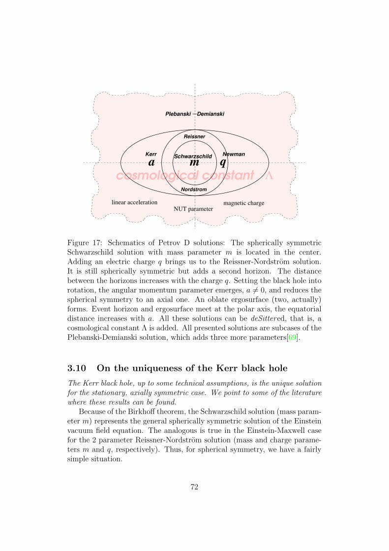
magnetic chargelinear accelerationNUT parameter

cosmological constant Λ

NewmanKerrSchwarzschild

m qa

Reissner

Nordstrom

Plebanski Demianski

Figure 17: Schematics of Petrov D solutions: The spherically symmetricSchwarzschild solution with mass parameter m is located in the center.Adding an electric charge q brings us to the Reissner-Nordstrom solution.It is still spherically symmetric but adds a second horizon. The distancebetween the horizons increases with the charge q. Setting the black hole intorotation, the angular momentum parameter emerges, a 6= 0, and reduces thespherical symmetry to an axial one. An oblate ergosurface (two, actually)forms. Event horizon and ergosurface meet at the polar axis, the equatorialdistance increases with a. All these solutions can be deSittered, that is, acosmological constant Λ is added. All presented solutions are subcases of thePlebanski-Demianski solution, which adds three more parameters[69].

3.10 On the uniqueness of the Kerr black hole

The Kerr black hole, up to some technical assumptions, is the unique solutionfor the stationary, axially symmetric case. We point to some of the literaturewhere these results can be found.

Because of the Birkhoff theorem, the Schwarzschild solution (mass param-eter m) represents the general spherically symmetric solution of the Einsteinvacuum field equation. The analogous is true in the Einstein-Maxwell casefor the 2 parameter Reissner-Nordstrom solution (mass and charge parame-ters m and q, respectively). Thus, for spherical symmetry, we have a fairlysimple situation.

72

In contrast, in the axially symmetric case, there does not exist a gener-alized Birkhoff theorem. The 2-parameter Kerr solution (mass and rotationparameters m and a, respectively), is just a particular solution for the axi-ally symmetric case. As we saw in Sec.3.8, the Kerr solution has very simplegravitoelectric and gravitomagnetic multipole moments (179,180). Numer-ous solutions are known that represent the exterior of matter distributionswith different multipole moments. The analogous is valid for the 3 parame-ter Kerr-Newman solution (parameters m, a, q), see Stephani et al.[180] andGriffiths & Podolsky[69].

However, one can show under quite general conditions that the Kerr-Newman metric represents the most general asymptotically flat, stationaryelectro-vacuum black hole solution (“no-hair theorem”), see Meinel’s shortreview[122]. Important contributions to the subject of black hole uniquenesswere originally made by Israel[90, 91], Carter[30, 31], Hawking & Ellis[78],Robinson[166, 167], and Mazur[120] (1967-1982), for details see the recentreview of Chrusciel et al.[38].

More recently Neugebauer and Meinel[130, 133] found a constructivemethod for proving the uniqueness theorem for the Kerr black hole met-ric. This was extended to the Kerr-Newman case by Meinel.[121] By inversescattering techniques, they showed how one can construct the Ernst potentialof the Kerr(-Newman) solution amongst the asymptotically flat, stationary,and axially symmetric (electro-)vacuum spacetimes surrounding a connectedKilling horizon.

Let us then eventually pose the following questions[27]:(i) Are axially symmetric, stationary vacuum solutions outside some mat-

ter distribution “Kerr”? The answer is “certainly not”, and it makessense to figure out ways to characterize the Kerr metric, see Sec.3.8.

(ii) Is the Kerr solution the unique axially symmetric, stationary vacuumblack hole? The answer is essentially “yes” (modulo some technicalissues)—see, for example Mazur[120].

The general tendency in the recent development of the subject is to useadditional scalar or other matter fields. They weaken the uniqueness theo-rems, which is probably not too surprising.

Let us conclude with a quotation that may make you curious to learnstill more about the beauty of the Kerr metric: We have many differentaxially symmetric solutions. The Kerr solution is characterized by “station-ary, axially symmetric, asymptotically flat, Petrov type D vacuum solution ofthe vanishing of the Simon tensor, admitting a rank-2 Killing-Stackel (KS)tensor of Segre type [(11)(11)] constructed from a (non-degenerate) rank-2Killing-Yano (KY) tensor”, see Hinoui et al.[87].

73

3.11 On interior solutions with material sources

To match the Kerr (vacuum) metric to a material source consistently is oneof the big unsolved problems. Only the rotating disc solution of Neugebauer& Meinel provides some hope.

This section is added in order to draw your attention to an unsolved prob-lem, to the solution of which you might want to contribute. Find a realisticmaterial source for the Kerr metric in the sense of an exact solution. Manyunsuccessful attempts have been made, see the early review of Krasinski[101]of 1978. More recently, in 2006, Krasinski[156] concludes “that a bright newidea is needed, as opposed to routine standard tricks tested so far.” Thisstatement was not made lightheartedly, Krasinski knows what he is talkingabout.

Many axially symmetric vacuum solutions were constructed. Quevedo &Mashhoon[161], for example, deformed the multipole moments of the Kerr(-Newman) metric and constructed appropriate solutions of the Einstein(-Maxwell) equation that describe the exterior gravitational field of a (charged)rotating mass. It is always the hope that somebody may find a suitable mat-ter distribution with the multipole moments of the Kerr solution—but thisdid not happen so far; for another approach see Marsh[115].

We are only aware of one exact solution that fits into this general context:It is the infinitesimally thin and rigidly rotating dust solution of Neugebauer& Meinel[131, 132] (1993). It is an exact analytical solution of the Einsteinequation with matter. It depends on 2 independent parameters, the radiusρ0 of the disk and its angular velocity Ω. Petroff & Meinel[151] developed,by means of an iterative procedure, a post-Newtonian approximation of thesolution that helps to understand the Newtonian limit.

We recall that in electrostatics in flat space, for example, we prescribean electric charge distribution and we are used to solve the correspondingboundary value problem within Maxwell’s theory. Similarly, Neugebauer &Meinel specified a very thin rotating disk of dust and solved the boundaryvalue problem within GR. This is a well-defined procedure. The problem is,however, that within a non-linear theory, such as GR, it is extremely hardto implement. Remarkably, for certain parameter values, the gravitationalfield of the disk approach the extremal Kerr case. Accordingly, there existsa certain relation to the Kerr problem. The desideratum would be to finda rotating matter distribution the external field of which coincides with thecomplete Kerr field.

Driven by the fact that the electrically charged Kerr solution, the Kerr-Newman solution, has a g-factor of 2, exactly like the electron (see also Pfister

74

& King[153]), Burinskii[24, 25] speculated that a soliton like solution of theDirac equation may be the source of the Kerr metric, see also Burinskii &Kerr[26]. Is that the “bright new idea” Krasinski was talking about? We donot know but a hard check of the Burinskii ansatz seems worthwhile.

4 Kerr beyond Einstein

In generalizations of Einstein’s theory of gravity, the Riemannian geometryof spacetime is often extended to a more general geometrical framework. Wedescribe two such examples in which the Kerr metric still plays a vital role.

4.1 Kerr metric accompanied by a propagating linearconnection

We display the Kerr metric with cosmological constant that, together withan explicitly specified torsion, represents an exact vacuum solution of thetwo field equations of the Poincare gauge theory of gravity with quadraticLagrangian.

In gauge theories of gravitation, see Blagojevic et al.[17], the linear con-nection becomes a field that is at least partially independent from the met-ric. It can be either metric-compatible, then it is a connection with values inthe Lie-algebra of the Lorentz group SO(1, 3) and the geometry is called aRiemann-Cartan geometry, or it can be totally independent, then it residesin a so-called metric-affine space and the connection is GL(4, R)-valued. Forsimplicity, we concentrate here on the former case, the Poincare gauge theoryof gravity, but the latter case is also treated in the literature[187, 11].

Let us shortly sketch the theory. Gauging the Poincare group leads to aspacetime with torsion Tα and curvature Rαβ (Riemann-Cartan geometry26):

Tα := Dϑα = dϑα + Γβα ∧ ϑβ =

1

2Tij

αdxi ∧ dxj , (182)

Rαβ := dΓαβ − Γαγ ∧ Γγβ = −Rβα =

1

2Rij

αβdxi ∧ dxj . (183)

Besides the coframe 1-form ϑα, the Lorentz connection 1-form Γαβ = Γiαβdxi =

−Γβα is a second field variable of the gauge theory. For a Riemannian space,torsion Tα = 0 and Γαβ becomes the Levi-Civita connection.

26Experimental limits of a possible torsion of spacetime were recently specified in aremarkable paper by Obukhov et al.,[142] see also the literature given there.

75

We choose a model Lagrangian quadratic in torsion and curvature, inactual fact (for ~ = 1, c = 1),

V = − 1

2κ(Tα ∧ ϑβ) ∧ ?(Tβ ∧ ϑα)− 1

2%Rαβ ∧ ?Rαβ , (184)

with Einstein’s gravitational constant κ (dimension length-squared) and adimensionless strong gravity coupling constant %. One can calculate the twovacuum field equations by varying with respect to ϑα and Γαβ. In 1988, forthese two field equations, a Kerr metric with torsion[10] was found as anexact solution.

We display here the orthonormal coframe and the torsion: The coframeϑα, in terms of Boyer-Lindquist coordinates (t, r, θ, φ), reads (in the conven-tions used in Ref.[10])

ϑ0 :=

√∆

ρ

(dt+ a sin2θ dφ

), (185)

ϑ1 :=ρ√∆dr , (186)

ϑ2 :=ρ√Fdθ , (187)

ϑ3 :=

√F sin θ

ρ

[adt+ (r2 + a2) dφ

]. (188)

As before, we have ρ2 := r2+a2cos2 θ. However, the other structure functionspick up a cosmological constant λ:

F := 1 +1

3λa2cos2 θ , ∆ := r2 + a2 − 2Mr − 1

3λr2(r2 + a2) . (189)

The corresponding metric is called a Kerr-deSitter metric. The coframe isorthonormal. Then the metric reads

g = −ϑ0 ⊗ ϑ0 + ϑ1 ⊗ ϑ1 + ϑ2 ⊗ ϑ2 + ϑ3 ⊗ ϑ3 . (190)

It is a characteristic feature of these exact solutions that even though theLagrangian (184) does not carry a cosmological constant, in the coframe andthe metric there emerges such a constant, namely λ := −3%/(4κ). This couldbe of potential importance for cosmology.

76

The torsion Tα of this stationary axially symmetric solution of the Poincaregauge theory reads (ϑαβ := ϑα ∧ ϑβ),

T 0 =ρ√∆

[−v1ϑ

01 +ρ√∆

[v2(ϑ02 − ϑ12) + v3(ϑ03 − ϑ13)

]− 2v4ϑ

23

],

T 1 = T 0 ,

T 2 =ρ√∆

[v5(ϑ02 − ϑ12) + v4(ϑ03 − ϑ13)

],

T 3 =ρ√∆

[−v4(ϑ02 − ϑ12) + v5(ϑ03 − ϑ13)

], (191)

with the following gravitoelectric and gravitomagnetic functions:

v1 =M

ρ4(r2 − a2cos2 θ) , v5 =

Mr2

ρ4; (192)

v2 = −Ma2rsin θcos θ

ρ5

√F , v3 =

Mar2sin θ

ρ5

√F , v4 =

Mar cos θ

ρ4.(193)

Metric and torsion of this exact solution are closely interwoven. Note, inparticular, that the leading gravitoelectric part in the torsion, for small a,is ∼ M/r2, a definitive Coulombic behavior proportional to the mass. Fora = 0, we find a Schwarzschild-deSitter solution with torsion.

One may legitimately ask, why is it that the Lagrangian (184) yieldsan exact solution with a Kerr-deSitter metric? The answer is simple: TheLagrangian was devised such that the torsion square-piece, in lowest orderin κ, encompasses a Newtonian approximation. This is already sufficient inorder to enable the existence of a Kerr-deSitter metric. One could even addanother torsion-square piece to V for getting an Einsteinian approximation,but this is not even necessary. Thus, only a Newtonian limit of some kindseems necessary for the emergence of the Kerr structure.

4.2 Kerr metric in higher dimensions and in string the-ory

There exist also Schwarzschild and Kerr metrics in higher dimensional space-times. These investigations are mainly motivated by supergravity and stringtheory.

Tangherlini[183] (1963) started to investigate higher dimensional Schwarzschildsolutions, with n − 1 spatial dimensions. He studied the (“planetary”) or-bits in an n-dimensional Schwarzschild field (“Sun”) and found that only forn = 4 we have stable orbits, see also Ortin[146]. According to Tangherlini,this is then the only case that is interesting for physics. Nowadays, however,

77

many physicists hypothesize that higher dimensions do exist because stringtheory suggests it.

Somewhat later, Myers and Perry[128] (1986) generalized these consid-erations to higher-dimensional Kerr metrics. In the meantime a plethoraof such higher-dimensional objects have been found, see Allahverdizadeh etal.[5] and Frolov & Zelnikov[64]. Recently Keeler et al.[97] investigated, inthe context of string theory, the separability of Klein-Gordon or Dirac fieldson top of a higher-dimensional Kerr type solutions. Lately Brihaye et al.[21],for example, discussed the exact solution of a 5d Myers-Perry black holes ascoupled to a to a massive scalar field. The physical interpretations of theseresults remain to be seen.

Acknowledgments

We are grateful to Wei-Tou Ni (Hsin-chu) for inviting us to contribute tohis Einstein volume. Georg Dautcourt (Berlin), Anne Franzen (Utrecht),Bahram Mashhoon (Columbia, Missouri), Reinhard Meinel (Jena), GernotNeugebauer (Jena), Hernando Quevedo (Mexico City), and Walter Simon(Vienna) helped us to understand gravitoelectromagnetism, the Kerr solu-tion, and more. We would like to thank Jens Boos (Cologne), Alberto Favaro(Oldenburg/Treviso), Eva Hackmann (Bremen), Gerald Marsh (Chicago),and Herbert Pfister (Tubingen) for valuable remarks. Our three referees,Steve Carlip (Davis), James Nester (Chung-li), and Dah-Wei Chiou (Taipei)helped us to avoid a number of slips. Our sincere thanks for their numeroussuggestions. We thank Mikael Ragstedt (Djursholm), librarian of the Mittag-Leffler Institute, for sending us a copy of Gullstand’s original paper[70] andfor providing information about Gullstrand.

78

Appendix

A Exterior calculus and computer algebra

We want to use as input the Papapetrou metric (93). We take the equivalentrepresentation in the form of the orthonormal coframe of the Eqs.(94) to(98). How such a Reduce-Excalc program can be set up, is demonstratedin Stauffer et al.[178] and in Socorro et al.[176], for the Einstein 3-form, seeHeinicke[82]:

%*****************************************************

% Coframe of Andress-Lewis-Papapetrou-Buchdahl metric

%*****************************************************

% file Buchdahl03.exi, 29 July 2014, fwh & chh

% in "Buchdahl03.exi";

load_package excalc;

off exp$

pform f=0, omega=0, gamma=0 $

fdomain f=f(rho,z), omega=omega(rho,z), gamma=gamma(rho,z) ;

coframe o(0) = sqrt(f) * (d t - omega * d phi),

o(1) = sqrt(f)**(-1) * exp(gamma) * d rho,

o(2) = sqrt(f)**(-1) * exp(gamma) * d z,

o(3) = sqrt(f)**(-1) * rho * d phi

with signature (1,-1,-1,-1);

displayframe;

frame e$

%*****************************************************

% Connection, curvature, and Einstein forms

%*****************************************************

pform conn1(a,b)=1, curv2(a,b)=2$

antisymmetric conn1, curv2$

factor o(0), o(1), o(2), o(3)$

conn1(-a,-b) := (1/2)*( e(-a)_|d o(-b) - e(-b)_|d o(-a)

- (e(-a)_|(e(-b)_|d o(-c))) * o(c))$

curv2(-a,b) := d conn1(-a,b) - conn1(-a,c) ^ conn1(-c,b)$

79

% Einstein tensor = Einstein 0-form

pform einstein3(a)=3, einstein0(a,b)=0$

symmetric einstein0$

einstein3(-a) := -(1/2) * curv2(b,-c) ^ # (o(-a) ^ o(-b) ^ o(c))$

einstein0(a,-b):= #( o(a) ^ einstein3(-b))$

on exp, gcd$

factor ^$

on nero;

einstein0(a,-b):= #( o(a) ^ einstein3(-b));

off nero;

% by inspection, we find

einstein0(1,-1) + einstein0(2,-2); % equals 0

einstein0(0,-0) - einstein0(3,-3); % eliminates gamma

out "Buchdahl03.exo";

load_package tri;

on tex;

on TeXBreak;

einstein0(a,-b):=einstein0(a,-b);

off tex;

einstein0(a,-b):=einstein0(a,-b);

omega:=0;

einstein0(a,-b):=einstein0(a,-b);

shut "Buchdahl03.exo";

;end;

80

References

[1] R. Adler, M. Bazin, and M. Schiffer, Introduction to General Relativity,2nd ed., McGraw-Hill, New York (1975). 36

[2] E. S. Akeley, The axially symmetric stationary gravitational field, Phil.Mag. 11, 322–330 (1931). 42

[3] E. S. Akeley, The rotating fluid in the relativity theory, Phil. Mag. 11,330–344 (1931). 42

[4] W. Alexandrow, Uber den kugelsymmetrischen Vakuumvorgang in derEinsteinschen Gravitationstheorie, Ann. Phys. (Berlin)27 377, 141–152(1923). 18

[5] M. Allahverdizadeh, J. Kunz and F. Navarro-Lerida, Charged RotatingBlack Holes in Higher Dimensions, J. Phys. Conf. Ser. 314, 012109(2011) [arXiv:1012.5052]. 78

[6] W. R. Andress, Some solutions of Einstein’s gravitational equations forsystems with axial symmetry, Proc. Roy. Soc. (London) A 126, 592–602(1930). 42

[7] R. Angelil and P. Saha, Clocks around Sgr A∗, Mon. Not. Roy. Astron.Soc. 444, 3780–3791 (2014) [arXiv:1408.0283]. 69

[8] R. Bach, Neue Losungen der Einsteinschen Gravitationsgleichungen. A.Das Feld in der Umgebung eines langsam rotierenden kugelahnlichenKorpers von beliebiger Masse in 1. und 2. Annaherung, MathematischeZeitschrift 13, 119–133 (1922). 42

[9] T. Backdahl and J. A. Valiente Kroon, Constructing “non-Kerrness” oncompact domains, J. Math. Phys. 53, 042503 (2012) [arXiv:1111.6019].70

[10] P. Baekler, M. Gurses, F. W. Hehl and J. D. McCrea, The exteriorgravitational field of a charged spinning source in the Poincare gaugetheory: a Kerr-Newman metric with dynamic torsion. Phys. Lett. A128, 245–250 (1988). 76

[11] P. Baekler and F. W. Hehl, Rotating black holes in metric-affine gravity,Int. J. Mod. Phys. D 15, 635–668 (2006) [arXiv:gr-qc/0601063]. 75

27We refer to the Annalen der Physik (formerly Leipzig, now Berlin), in the way thejournal is organized in the Wiley Online Lirary [WileyOnlineLibrary.Ann.Phys.(Berlin)].

81

[12] R. Beig and W. Simon, The stationary gravitational field near spatialinfinity, Gen. Rel. Grav. 12, 1003–1013 (1980). 70

[13] J. D. Bekenstein, Extraction of energy and charge from a black hole,Phys. Rev. D 7, 949–953 (1973). 58

[14] R. Bergamini and S. Viaggiu, A novel derivation for Kerr metricin Papapetrou gauge, Class. Quant. Grav. 21, 4567 (2004) [arXiv:gr-qc/0305035]. 49

[15] D. Bini and R. T. Jantzen, Stationary spacetimes and the Simon tensor,Nuovo Cim. B 119, 863–873 (2004) [arXiv:gr-qc/0411051]. 70

[16] G. D. Birkhoff, Relativity and Modern Physics, Harvard UniversityPress, Cambridge, MA (1923) p.253. 18

[17] M. Blagojevic and F. W. Hehl (eds.), Gauge Theories of Gravitation: AReader with Commentaries, Imperial College Press, London (2013). 75

[18] W. B. Bonnor and B. R. Steadman, The gravitomagnetic clock effect,Class. Quantum Grav. 16, 1853–1861 (1999). 68

[19] J. Boos, Curvature (pseudo-)invariants of the Kerr solution. Computeralgebra programs (12 July 2014), see also [arXiv:1412.1958 51 pages(2014)]. 68

[20] R. H. Boyer and R. W. Lindquist, Maximal analytic extension of theKerr metric, J. Math. Phys. 8, 265–281 (1967). 60

[21] Y. Brihaye, C. Herdeiro and E. Radu, Myers-Perry black holes withscalar hair and a mass gap, [arXiv:1408.5581 11 pages (2014)]. 78

[22] D. Brill, History of a black hole horizon, Grav. & Cosmol. 20, 165–170(2014). 26

[23] H. A. Buchdahl, Seven Simple Lectures on General Relativity Theory,Wiley, New York (1981). 44, 48

[24] A. Burinskii, Complex structure of the four-dimensional Kerr geome-try: stringy system, Kerr theorem, and Calabi-Yau twofold. Adv. HighEnergy Phys. 2013, 509749 (2013) [arXiv:1211.6021]. 75

[25] A. Burinskii, Emergence of the Dirac equation in the solitonic source ofthe Kerr spinning particle [arXiv:1404.5947, 4 pages (2014)]. 75

82

[26] A. Burinskii and R. P. Kerr, Nonstationary Kerr congruences, [arXiv:gr-qc/9501012]. 75

[27] S. Carlip, private communication (September 2014). 73

[28] S. Carlip, Black Hole Thermodynamics, Int. J. Mod. Phys. D 23,1430023 (2014) [arXiv:1410.1486]. 59

[29] S. Carroll, Spacetime and Geometry. An Introduction to General Rela-tivity, Addison Wesley, San Francisco (2004). 26, 27

[30] B. Carter, Black hole equilibrium states, In Ref.[45], pp.57–214 (1973).60, 73

[31] B. Carter, Global and local problems solved by the Kerr metric. InRef.[190], pp.95–114 (2009). 73

[32] C. Cherubini, D. Dini, S. Cappozziello and R. Ruffini, Second orderscalar invariants of the Riemann tensor: applications to black hole space-times, Int. J. Mod. Phys. D 11, 827–841 (2002) [arXiv:gr-qc/0302095].68

[33] I. Ciufolini, S. Kopeikin, B. Mashhoon and F. Ricci, On the gravit-omagnetic time delay, Phys. Lett. A 308, 101–109 (2003) [arXiv:gr-qc/0210015]. 68

[34] I. Ciufolini and E. C. Pavlis, A confirmation of the general relativisticprediction of the Lense-Thirring effect, Nature 431, 958–960 (2004). 42

[35] I. Ciufolini, E. Pavlis, F. Chieppa, E. Fernandes-Vieria, and J. Perez-Mercader, Test of general relativity and the measurement of the Lense-Thirring effect with two earth satellites, Science 279, 2100–2104 (1998).42

[36] I. Ciufolini and J. A. Wheeler, Gravitation and Inertia, Princeton Univ.Press, Princeton, NJ (1995). 68

[37] J. M. Cohen and B. Mashhoon, Standard clocks, interferometry, andgravitomagnetism, Phys. Lett. A 181, 353–358 (1993). 68

[38] P. T. Chrusciel, J. L. Lopes Costa and M. Heusler, Stationary blackholes: uniqueness and beyond, Living Rev. Rel. 15, no.7, 1–69 (2012).[arXiv:1205.6112]. 39, 73

83

[39] N. Dadhich, A novel derivation of the rotating black hole metric, Gen.Rel. Grav. 45, 2383–2388 (2013) [arXiv:1301.5314]. 49

[40] G. Dautcourt, Race for the Kerr field, Gen. Rel. Grav. 41, 1437–1454(2009) [arXiv:0807.3473]. 44

[41] F. de Felice and M. Bradley, Rotational anisotropy and repulsive effectsin the Kerr metric, Class. Quant. Grav. 5, 1577–1585 (1988). 68

[42] F. de Felice and C. J. S. Clarke, Relativity on curved manifolds, Cam-bridge Univ. Press, Cambridge, UK (1990). 68

[43] W. de Sitter, On Einstein’s theory of gravitation, and its astronomicalconsequences, first paper and second paper, Mon. Not. Roy. Astron. Soc.76, 699–728 (1916), 77, 155–184 (1916). 42

[44] C. DeWitt and B. DeWitt (eds.), Relativity, Groups and Topology, LesHouches Summer School 1963, Gordon and Breach, New York (1964).92

[45] C. DeWitt and B. S. DeWitt (eds.), Black Holes, Les Houches SummerSchool 1972, Gordon and Breach, New York (1973). 83

[46] C. Doran, New form of the Kerr solution, Phys. Rev. D 61, 067503(2000) [arXiv:gr-qc/9910099].

[47] J. Droste, The field of a single centre in Einstein’s theory of gravitation,and the motion of a particle in that field, Gen. Rel. Grav. 34, 1545–1563(2002); translation of the Dutch original of 1916. 49

[48] J. Ehlers and A. Krasinski, Comment on the paper by J. T. Jebsenreprinted in Gen. Rel. Grav 37, 2253–2259 (2005), Gen. Rel. Grav 38,1329–1330 (2006). 18

[49] A. Einstein, Uber das Relativitatsprinzip und die aus demselben gezoge-nen Folgerungen. In [177] pp.411–462 (1907). 18

[50] A. Einstein, The Meaning of Relativity, 5th ed., Princeton Univ. Press,Princeton, NJ (1992) [first published in 1922]. 19

[51] A. Einstein, The Collected Papers of Albert Einstein, Vol. 8: The BerlinYears: Correspondence, 1914–1918, Part A: 1914–1917, Part B: 1918.R. Schulmann, A. J. Kox, et al. (eds.), Princeton Univ. Press, Princeton,NJ (1998). 13

84

[52] J. Eisenstadt: The early interpretation of the Schwarzschild solution, in:Einstein and the History of General Relativity, D. Howard & J. Stachel(eds.), Birkhauser, Boston (1989), pp.213–233. 16

[53] F. J. Ernst, New formulation of the axially symmetric gravitational fieldproblem, Phys. Rev. 167, 1175–1179 (1968). 22

[54] F. J. Ernst, New formulation of the axially symmetric gravitational fieldproblem. II, Phys. Rev. 168, 1415–1417 (1968); Erratum 172, 1850. 44,47

71

[55] C. W. F. Everitt et al., Gravity Probe B: Final results of a space ex-periment to test general relativity . Phys. Rev. Lett. 106, 221101 (2011)[arXiv:1105.3456]. 42

[56] H. Falcke and F. W. Hehl (eds.), The Galactic Black Hole, Lectureson General Relativity and Astrophysics, IoP Publishing, Bristol, UK(2003). 3, 87

[57] F. de Felice and C. J. S. Clarke: Relativity on curved manifolds. Cam-bridge Univ. Press, Cambridge, UK (1990). 44

[58] P. G. Ferreira, Perfect Theory: A Century of Geniuses and the Battleover General Relativity, Houghton Mifflin Harcourt, Boston, MA (2014).44

[59] D. Finkelstein: Past-future asymmetry of the gravitational field of apoint particle, Phys. Rev. 110, 965–967 (1958). 26

[60] L. Flamm: Beitrage zur Einsteinschen Gravitationstheorie, Phys. Zeits.17, 448–454 (1916). 17

[61] J. Fleischer, J. Grabmeier, F. W. Hehl, and W. Kuchlin (eds.): Com-puter algebra in science and engineering, World Scientific, Singapore(1995). 93

[62] A. Franzen, Boundedness of massless scalar waves on Reissner-Nordstrom interior backgrounds, [arXiv:1407.7093]. 64

[63] A. V. Frolov and V. P. Frolov, Rigidly rotating ZAMO surfaces in theKerr spacetime, [arXiv:1408.6316, 11 pages (2014)]. 57

[64] V. P. Frolov and A. Zelnikov, Introduction to Black Hole Physics, OxfordUniv. Press, Oxford, UK (2011). 52, 78

85

[65] A. Garcıa, F. W. Hehl, C. Heinicke and A. Macıas, The Cotton tensorin Riemannian space-times. Class. Quant. Grav. 21, 1099–1118 (2004)[arXiv:gr-qc/0309008]. 70

[66] H. Garcia-Compean and V. S. Manko, Are maximal analytic exten-sions of the Kerr and Kerr-Newman spacetimes physically meaningful?[arXiv:1205.5848]. 53

[67] R. P. Geroch, Multipole moments. II. Curved space, J. Math. Phys. 11,2580–2588 (1970). 69

[68] J. Grabmeier, E. Kaltofen, and V. Weispfenning (eds.), Computer Al-gebra Handbook. Foundations, Applications, Systems. Springer, Berlin(2003). 44

[69] J. B. Griffiths and J. Podolsky, Exact Space-Times in Einstein’s GeneralRelativity, Cambridge Univ. Press, Cambridge, UK (2009). 35, 44, 48,72, 73

[70] A. Gullstrand, Allgemeine Losung des statischen Einkorperproblems inder Einsteinschen Gravitationstheorie (General solution of the staticone-body problem in Einstein’s gravitational theory), Arkiv. Mat. As-tron. Fys. 16, 1–15 (1922) [presented on 25 May 1921]. 20, 78

[71] E. Hackmann and C. Lammerzahl, A generalized gravitomagnetic clockeffect, Phys. Rev. D 90, 044059 (2014) [arXiv:1406.6232]. 69

[72] E. Hackmann, C. Lammerzahl, Y. N. Obukhov, D. Puetzfeld andI. Schaffer, Motion of spinning test bodies in Kerr spacetime, Phys. Rev.D 90, 064035 (2014) [arXiv:1408.1773]. 52

[73] R. O. Hansen, Multipole moments of stationary spacetimes, J. Math.Phys. 15, 46–52 (1974). 69

[74] A. Harvey, On Einstein’s Path: Essays in Honor of Engelbert Schucking,Springer, New York (1999). 87

[75] I. Hauser and F. J. Ernst, A homogeneous Hilbert problem for theKinnersley-Chitre transformations, J. Math. Phys. 21, 1126–1149(1980). 49

[76] I. Hauser and F. J. Ernst, Proof of a Geroch conjecture, J. Math. Phys.22, 1051–1063 (1981). 49

86

[77] I. Hauser and F. J. Ernst, A new proof of an old conjecture, in Ref.[164]pp.165–214 (1987). 49

[78] S. W. Hawking and G. F. R. Ellis, The Large Scale Structure of Space-time, Cambridge Univ. Press, Cambridge, UK (1973). 60, 73

[79] A. C. Hearn, Reduce User’s Manual, Version 3.5, RAND PublicationCP78 (Rev. 10/93). The RAND Corporation, Santa Monica, CA 90407-2138, USA (1993). Nowadays Reduce is freely available for download;for details see [reduce-algebra.com] and [sourceforge.net]. 44

[80] F. W. Hehl, A. Macıas, E. W. Mielke, Yu. N. Obukhov, On the struc-ture of the energy-momentum and the spin currents in Dirac’s electrontheory, in Ref.[74] pp.257–274 (1999). 66

[81] F. W. Hehl and Yu. N. Obukhov, Foundations of Classical Electrody-namics: Charge, flux, and metric. Birkhauser, Boston (2003). 35, 67

[82] C. Heinicke, The Einstein 3-form Gα and its equivalent 1-Form Lα inRiemann-Cartan space. Gen. Rel. Grav. 33, 1115–1130 (2001) [arXiv:gr-qc/0012037]. 79

[83] C. Heinicke and F. W. Hehl, The Schwarzschild black hole: a generalrelativistic introduction. In Ref.[56], pp.3–34 (2003). 3

[84] R. C. Henry, Kretschmann scalar for a Kerr-Newman black hole, Astro-phys. J. 535, 350–353 (2000) [arXiv:astro-ph/9912320]. 68

[85] M. Heusler, Black Hole Uniqueness Theorems, Cambridge Univ. Press,Cambridge, UK (1996). 48, 59

[86] D. Hilbert, Die Grundlagen der Physik. (Zweite Mitteilung), Nachr.Gesell. Wissensch. zu Gottingen, Math.-Phys. Klasse, pp.53–76 (1917).17, 18

[87] K. Hinoue, T. Houri, C. Rugina and Y. Yasui, General Wahlquist metricsin all dimensions, [arXiv:1402.6904]. 73

[88] A. D. Ionescu and S. Klainerman, On the uniqueness of smooth, station-ary black holes in vacuum, [arXiv0711.0040: 60 pages]. 70

[89] L. Iorio, An assessment of the systematic uncertainty in present and fu-ture tests of the Lense-Thirring effect with satellite laser ranging, SpaceSci. Rev. 148, 363–381 (2009) [arXiv:0809.1373]. 42

87

[90] W. Israel, Event horizons in static vacuum space-times, Phys. Rev. 164,1776–1779 (1967). 73

[91] W. Israel, Event horizons in static electrovac space-times, Comm. Math.Phys. 8, 245–260 (1968). 73

[92] L. Iorio, H. I. M. Lichtenegger, M. L. Ruggiero and C. Corda, Phe-nomenology of the Lense-Thirring effect in the Solar System, Astrophys.Space Sci. 331, 351–395 (2011) [arXiv:1009.3225]. 42

[93] J. N. Islam, Rotating fields in general relativity, Cambridge Univ. Press,Cambridge, UK (1985). 48

[94] J. D. Jackson, Classical Electrodynamics, 3rd edition, Wiley, New York(1999). 47

[95] J. T. Jebsen, On the general spherically symmtric solutions of Einstein’sgravitational equations in vacuo, Gen. Rel. Grav. 37, 2253–2259 (2005);reprinted, the original was published in German in 1921. 18

[96] N. V. Johansen and F. Ravndal, On the discovery of Birkhoff’s theorem,Gen. Rel. Grav. 38, 537–540 (2006) [arXiv:physics/0508163]. 18

[97] C. Keeler and F. Larsen, Separability of black holes in string theory,JHEP 1210, 152 (2012) [arXiv:1207.5928]. 78

[98] R. P. Kerr, Gravitational field of a spinning mass as an example ofalgebraically special metrics, Phys. Rev. Lett. 11, 237–238 (1963). 43

[99] R. P. Kerr, Discovering the Kerr and Kerr-Schild metrics, in [190] ,pp.38–72 (2009) [arXiv:arXiv:0706.1109]. 43

[100] D. Kramer und G. Neugebauer, Zu axialsymmetrischen stationarenLosungen der Einsteinschen Feldgleichungen fur das Vakuum, Comm.Math. Phys. 10, 132–139 (1968). 44, 47

[101] A. Krasinski, Ellipsoidal spacetimes, sources for the Kerr metric, Ann.Phys. (NY) 112, 22–40 (1978). 74

[102] A. Krasinski, G. F. R. Ellis, M. A. H. MacCallum (eds.), Golden Oldiesin General Relativity. Hidden Gems, Springer, Heidelberg (2013). Thisbook contains 14 of the 58 “Golden Oldie” articles that had been orig-inally republished (partly translated into the English) in the journalGeneral Relativity and Gravitation. 89, 92

88

[103] C. Lammerzahl, C. W. F. Everitt, and F. W. Hehl (eds.), Gyros,Clocks, Interferometers. . . : Testing Relativistic Gravity in Space. Lec-ture Notes in Physics Vol. 562, Springer, Berlin (2001). 68, 90

[104] K. Lanczos, Ein vereinfachendes Koordinatensystem fur die Einstein-schen Gravitationsgleichungen, Phys. Zeits. 23, 537–539 (1922). 17

[105] K. Lanczos, Uber eine stationare Kosmologie im Sinne der Einstein-schen Gravitationstheorie, Z. Physik 21, 73–110 (1924). 42

[106] L. D. Landau and E. M. Lifshitz: The Classical Theory of Fields, Vol.2of Course of Theoretical Physics, p. 281; transl. from the Russian, 4threv. English ed., Elsevier, Amsterdam (1975). 13

[107] J. Lense and H. Thirring, Uber den Einfluss der Eigenrotation der Zen-tralkorper auf die Bewegung der Planeten und Monde nach der Einstein-schen Gravitationstheorie, Physikalische Zeitschrift 19, 156–163 (1918);an English translation is provided in Ref.[119], see also Ref.[102], Chap-ter 6. 41

[108] T. Levi-Civita, ds2 einsteiniani in campi newtoniani. Seven notes inRendiconti della R. Academia dei Lincei, 27, 28, 29 (1917–1919). 41,42

[109] T. Lewis, Some special solutions of the equations of axially symmetricgravitational fields, Proc. Roy. Soc. Lond. A 136, 176–192 (1932). 42

[110] V. S. Manko and H. Garcia-Compean, On non-disk geometry ofr = 0 in Kerr-de Sitter and Kerr-Newman-de Sitter spacetimes,[arXiv:1406.3434]. 53

[111] M. Mars, A Space-time characterization of the Kerr metric, Class.Quant. Grav. 16, 2507–2523 (1999) [arXivgr-qc/9904070]. 70

[112] M. Mars, Uniqueness properties of the Kerr metric, Class. Quant. Grav.17, 3353–3373 (2000) [arXiv:gr-qc/0004018]. 70

[113] M. Mars and J. M. M. Senovilla, A spacetime characterization of theKerr-NUT-(A)de Sitter and related metrics, [arXiv:1307.5018, 39 pages(2013)]. 70

[114] G. E. Marsh, The Infinite red-shift surfaces of the Kerr solution, 55

[arXiv:gr-qc/0702114, 23 pages (2007)].

89

[115] G. E. Marsh: Rigid rotation and the Kerr metric [arXiv:1404.5297, 15pages (2014)]. 74

[116] B. Mashhoon, Gravitoelectromagnetism: A Brief Review [arXiv:gr-qc/0311030]. 65, 66

[117] B. Mashhoon, F. Gronwald and H. I. M. Lichtenegger, Gravitomag-netism and the clock effect, Lect. Notes Phys. 562, 83–108 (2001), seeRef.[103] [arXiv:gr-qc/9912027]. 68

[118] B. Mashhoon, F. Gronwald, D. S. Theiss, On measuring gravitomag-netism via spaceborne clocks: a gravitomagnetic clock effect, Ann. Phys.(Lpz.) 8, 135–152 (1999) [arXiv:gr-qc/9804008]. 68

[119] B. Mashhoon, F. W. Hehl and D. S. Theiss, On the gravitational effectsof rotating masses: The Thirring-Lense papers. Gen. Rel. Grav. 16, 711–749 (1984). 89

[120] P. O. Mazur, Proof of uniqueness of the Kerr-Newman black hole solu-tion, J. Phys. A 15, 3173–3180 (1982). 73

[121] R. Meinel, Constructive proof of the Kerr-Newman black hole unique-ness including the extreme case, Class. Quant. Grav. 29, 035004 (2012)[arXiv:1108.4854]. 73

[122] R. Meinel, A physical derivation of the Kerr-Newman black hole solu-tion, 73

[arXiv:1310.0640, 8 pages (2013)].

[123] R. Meinel, M. Ansorg, A. Kleinwachter, G. Neugebauer and D. Petroff,Relativistic Figures of Equilibrium, Cambridge Univ. Press, Cambridge,UK (2008). 48, 69, 91

[124] F. Melia, Cracking the Einstein Code. Relativity and the Birth of BlackHole Physics, Univ. of Chicago Press, Chicago (2009). 43

[125] J. Michell, On the means of discovering the distance, magnitude, &c.of the fixed stars..., Phil. Trans. R. Soc. London 74, 35–57 (1784). 24

[rstl.royalsocietypublishing.org/content/74.toc].

[126] G. Mie, Die Einfuhrung eines vernunftgemaßen Koordinatensystemsin die Einsteinsche Gravitationstheorie und das Gravitationsfeld einerschweren Kugel, Ann. Phys. (Berlin) 367, 47–74 (1920). 21

90

[127] C.W. Misner, K.S. Thorne, and J.A. Wheeler: Gravitation. Freeman,San Francisco (1973). 13, 14

[128] R. C. Myers and M. J. Perry, Black holes in higher dimensional space-times, Ann. Phys. (NY) 172, 304–347 (1986). 78

[129] R. Narayan and J. E. McClintock, Observational evidence for blackholes, to be published in General Relativity and Gravitation: A Centen-nial Perspective, A. Ashtekar et al. (eds.), Cambridge University Press,Cambridge (2014/15) [arXiv:1312.6698]. 26

[130] G. Neugebauer, Rotating bodies as boundary value problems, Ann.Phys. (Leipzig) 9, 342–354 (2000). 73

[131] G. Neugebauer and R. Meinel, The Einsteinian gravitational field ofa rigidly rotating disk of dust, Astrophys. J. 414, L97–L99 (1993); seealso Sec.2.3 of Ref.[123]. 74

[132] G. Neugebauer and R. Meinel, General relativistic gravitational field ofa rigidly rotating disk of dust: Solution in terms of ultraelliptic func-tions, Phys. Rev. Lett. 75, 3046–3047 (1995) [arXiv:gr-qc/0302060]. 74

[133] G. Neugebauer and R. Meinel, Progress in relativistic gravitational the-ory using the inverse scattering method, J. Math. Phys. 44, 3407–3429(2003) [arXiv:gr-qc/0304086]. 73

[134] E. T. Newman, E. Couch, K. Chinnapared, A. Exton, A. Prakash,R. Torrence: Metric of a rotating, charged mass, J. Math. Phys. 6, 918–919 (1965). 71

[135] E. T. Newman, A. I. Janis, Note on the Kerr spinning-particle metric,J. Math. Phys. 6, 915–917 (1965). 71

[136] I. Newton, The Principia: mathematical principles of natural philoso-phy. Translation by B. I. Cohen, A. Whitman, and J. Budenz. Univeristyof California Press, Berkeley (1999). 3

[137] W. T. Ni and M. Zimmermann, Inertial and gravitational effects in theproper reference frame of an accelerated, rotating observer, Phys. Rev.D 17, 1473–1476 (1978). 65

[138] W. T. Ni, Searches for the role of spin and polarization in gravity,Rept. Prog. Phys. 73, 056901 (2010) [arXiv:0912.5057]. 66, 67

91

[139] W. T. Ni, Rotation, Equivalence Principle, and GP-B Experiment,Phys. Rev. Lett. 107, 051103 (2011) [arXiv:1105.4305]. 67

[140] G. Nordstrom, On the energy of the gravitational field in Einstein’stheory, Proc. Kon. Ned. Akad. Wet. 20, 1238–1245 (1918). 18

[141] Y. N. Obukhov and F. W. Hehl, On the relation between quadraticand linear curvature Lagrangians in Poincare gauge gravity, Acta Phys.Polon. B 27, 2685–2694 (1996) [arXiv:gr-qc/9602014]. 68

[142] Y. N. Obukhov, A. J. Silenko and O. V. Teryaev, Spin-torsion couplingand gravitational moments of Dirac fermions: theory and experimentalbounds [arXiv:1410.6197, 28 pages (2014)]. 75

[143] H. C. Ohanian and R. Ruffini, Gravitation and Spacetime, 3rd ed.,Cambridge Univ. Press, New York, NY (2013). 42

[144] B. O’Neill, The Geometry of Kerr Black Holes, Peters, Wellesley, MA1995. 44

[145] J. R. Oppenheimer, H. Snyder: On continued gravitational contraction,Phys. Rev. 56, 455–459 (1939). 39

[146] T. Ortın, Gravity and Strings, Cambridge Univ. Press, Cambridge, UK(2004). 77

[147] P. Painleve, La mecanique classique et la theorie de la relativite (Clas-sical mechanics and relativity theory), C. R. Acad. Sci. (Paris) 173,677–680 (1921) [presented on 24 October 1921]. 20

[148] A. Papapetrou, Eine rotationssymmetrische Losung in der allgemeinenRelativitatstheorie, Ann. Phys. (Berlin) 447, 309–315 (1953). 43

[149] R. Penrose, Conformal treatment of infinity, in Ref.[44], pp. 563–584(1964); reprinted in Gen. Rel. Grav. 43, 901–922 (2011). 26

[150] R. Penrose, The Road to Reality. A Complete Guide to the Laws ofthe Universe, Knopf, New York (2005). 25, 64

[151] D. Petroff and R. Meinel, The post-Newtonian approximation of therigidly rotating disc of dust to arbitrary order, Phys. Rev. D 63, 064012(2001) [arXiv:gr-qc/0101081]. 74

[152] A. Z. Petrov, The classification of spaces defining gravitational fields.Translation from the Russian original of 1954, in Ref.[102], Chapter 4,see also Gen. Rel. Grav. 32, 1665–1685 (2000). 43

92

[153] H. Pfister and M. King, The gyromagnetic factor in electrodynamics,quantum theory and general relativity, Class. Quantum Grav. 20, 205–213 (2003). 75

[154] F. A. E. Pirani, Invariant formulation of gravitational radiation theory,Phys. Rev. 105, 1089–1099 (1957). 43

[155] J. F. Plebanski and M. Demianski, Rotating, charged uniformly accel-erated mass in general relativity, Annals of Physics (NY) 98, 98–127(1976). 49

[156] J. Plebanski and A. Krasinski, An Introduction to General Relativityand Cosmology, Cambridge Univ. Press, Cambridge, UK (2006). 74

[157] F. Pretorius and W. Israel: Quasi-spherical light cones of the Kerrgeometry, Class. Quant. Grav. 15, 2289–2301 (1998). 49

[158] R. A. Puntigam, E. Schrufer, and F. W. Hehl: The use of computeralgebra in Maxwell’s theory, in Ref.[61] pp.195–211 (1995), [arXiv:gr-qc/9503023]. 35

[159] H. Quevedo, General static axisymmetric solution of Einstein’s vacuumfield equations in prolate spheroidal coordinates, Phys. Rev. D 39, 2904–2911 (1989). 69

[160] H. Quevedo, Multipole moments in general relativity—Static and sta-tionary vacuum solutions— Fortschr. Phys./Progr. Phys. 38, 733–840(1990). 44, 69

[161] H. Quevedo and B. Mashhoon, Generalization of Kerr spacetime, Phys.Rev. D 43, 3902–3906 (1991). 69, 74

[162] S. Rahman and M. Visser, Spacetime geometry of static fluid spheres,Class. Quant. Grav. 19, 935–952 (2002) [arXiv:gr-qc/0103065]. 38

[163] H. Reissner: Uber die Eigengravitation des elektrischen Feldes nach derEinsteinschen Theorie, Ann. Phys. (Berlin) 355, 106–120 (1916). 18

[164] W. Rindler and A. Trautman (eds.), Gravitation and Geometry,Festschrift for I. Robinson, Bibliopolis, Naples, Italy (1987). 87

[165] W. Rindler, Relativity. Special, General, and Cosmological, OxfordUniv. Press, Oxford, UK (2001). 13, 57, 65, 69

93

[166] D. C. Robinson, Uniqueness of the Kerr black hole, Phys. Rev. Lett.34, 905–906 (1975). 73

[167] D. C. Robinson, Four decades of black hole uniqueness theorems. InRef.[190], pp.115–142 (2009).

[168] R. H. Sanders, Revealing the Heart of the Galaxy, the Milky Way andits black hole, Cambridge Univ. Press, Cambridge, UK (2014). 73

[169] M. A. Scheel and K. S. Thorne, Geometrodynamics: the nonlinear dy-namics of curved spacetime, Phys. Usp. 57, 342–351 (2014) [Usp. Fiz.Nauk 184, no. 4, 367–378 (2014)]. 25

[170] J. A. Schouten, Ricci-Calculus, 2nd ed. Springer, Berlin (1954). 66

[171] K. Schwarzschild, Gesammelte Werke/Collected Works, Vols.1, 2, and3. Edited by H. H. Voigt, Springer, Berlin (1992). 13

[172] K. Schwarzschild, Uber das Gravitationsfeld eines Massenpunktes nachder Einsteinschen Theorie (On the gravitational field of a mass pointaccording to Einstein’s theory), Sitzungsber. Preuss. Akad. Wiss. Berlin,pp.189–196 (1916). 16

[173] K. Schwarzschild, Uber das Gravitationsfeld einer Kugel aus inkom-pressibler Flussigkeit nach der Einsteinschen Theorie (On the gravita-tional field of a ball of an incompressible fluid according to Einstein’stheory), Sitzungsber. Preuss. Akad. Wiss. Berlin, pp.424–434 (1916). 16

[174] W. Simon, Characterizations of the Kerr metric, Gen. Relativ. Grav.16, 465–476 (1984). 17, 38

[175] W. Simon, The multiple expansion of stationary Einstein-Maxwellfields, J. Math. Phys. 25, 1035–1038 (1984). 70

[176] J. Socorro, A. Macias, and F. W. Hehl, Computer algebra in gravity:Reduce-Excalc programs for (non-)Riemannian space-times. I, Comput.Phys. Commun. 115, 264–283 (1998) [arXiv:gr-qc/9804068]. 70

[177] J. Stark (ed.), Jahrbuch der Radioaktivitat und Elektronik, Vol.4(1907). Hirzel, Leipzig (1908). 46, 79

[178] D. Stauffer, F. W. Hehl, N. Ito, V. Winkelmann, and J. G. Zabolitzky,Computer Simulation and Computer Algebra. Lectures for Beginners,3rd ed., Springer, Berlin (1993). 84

94

[179] H. Stephani, General Relativity. An introduction to the theory of thegravitational field, 2nd ed., Cambridge Univ. Press, Cambridge, UK(1990). 46, 79

[180] H. Stephani, D. Kramer, M. A. H. MacCallum, C. Hoenselaers, andE. Herlt, Exact Solutions to Einstein’s Field Equations, 2nd ed., Cam-bridge Univ. Press, Cambridge, UK (2003). 41

[181] S. Sternberg, Curvature in Mathematics and Physics, Dover, Mineola,NY (2012). 44, 69, 70, 73

[182] N. Straumann, General Relativity, 2nd ed., Springer, Dordrecht (2013).44, 51

[183] F. R. Tangherlini, Schwarzschild field in n dimensions and the dimen-sionality of space problem, Nuovo Cim. 27, 636–651 (1963).

[184] W. J. van Stockum, The gravitational field of a distribution of particlesrotating about an axis of symmetry, Proc. Roy. Soc. Edinburgh A 57,135–154 (1937). 77

[185] M. Visser, Heuristic approach to the Schwarzschild geometry, Int. J.Mod. Phys. D 14, 2051 (2005) [arXiv:gr-qc/0309072]. 43

[186] M. Visser, The Kerr spacetime—a brief introduction, in Ref.[190], pp.3–37 (2009) [arXiv:0706.0622]. 19

[187] E. J. Vlachynsky, R. Tresguerres, Y. N. Obukhov and F. W. Hehl, AnAxially symmetric solution of metric affine gravity, Class. Quant. Grav.13, 3253–3259 (1996) [arXiv:gr-qc/9604035]. 49

[188] H. Weyl, Zur Gravitationstheorie, Ann. Phys. (Berlin) 359, 117–145(1917); an English translation is provided in Gen. Rel. Grav. 44, 779–810 (2012). 75

[189] C. M. Will, The Confrontation between General Relativity and Experi-ment. Living Rev. Relativity 17, no.4 (2014) [arXiv:1403.7377]. 17, 18,41

[190] D. L. Wiltshire, M. Visser and S. M. Scott (eds.), The Kerr Spacetime.Rotating Black Holes in General Relativity, Cambridge Univ. Press,Cambridge, UK (2009). 6, 42

[191] S. Wolfram, Mathematica, Wolfram Research, Inc., Mathematica Edi-tion: Version 9.0, Champaign, IL (2013). 83, 88, 94, 95

95

[192] W. W. Wong, A space-time characterization of the Kerr-Newman met-ric, Annales Henri Poincare (Birkhauser, Basel) 10, 453–484 (2009)[arXiv:0807.1904]. 44

96