school of science and humanities department of mathematics

SCHOOL OF SCIENCE AND HUMANITIES

DEPARTMENT OF MATHEMATICS

UNIT – I – CURVES AND SURFACES – SMT5204

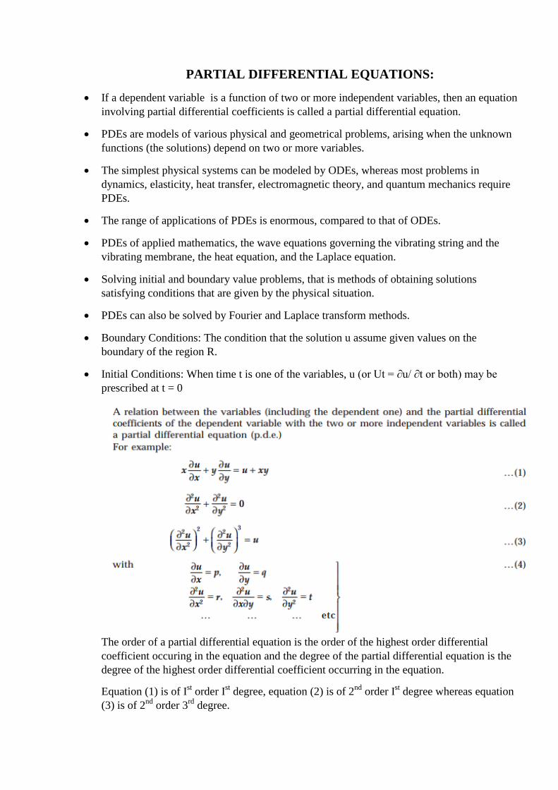
PARTIAL DIFFERENTIAL EQUATIONS:

If a dependent variable is a function of two or more independent variables, then an equation

involving partial differential coefficients is called a partial differential equation.

PDEs are models of various physical and geometrical problems, arising when the unknown

functions (the solutions) depend on two or more variables.

The simplest physical systems can be modeled by ODEs, whereas most problems in

dynamics, elasticity, heat transfer, electromagnetic theory, and quantum mechanics require

PDEs.

The range of applications of PDEs is enormous, compared to that of ODEs.

PDEs of applied mathematics, the wave equations governing the vibrating string and the

vibrating membrane, the heat equation, and the Laplace equation.

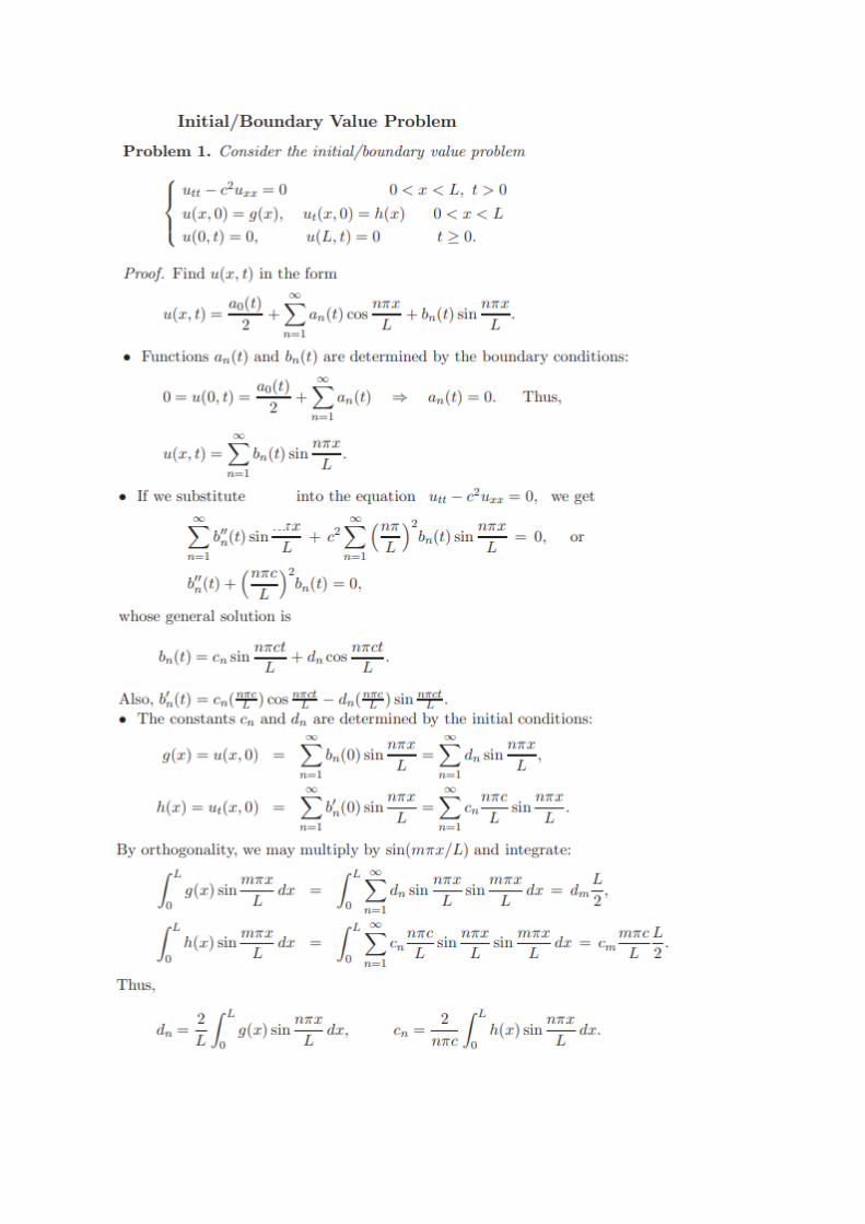
Solving initial and boundary value problems, that is methods of obtaining solutions

satisfying conditions that are given by the physical situation.

PDEs can also be solved by Fourier and Laplace transform methods.

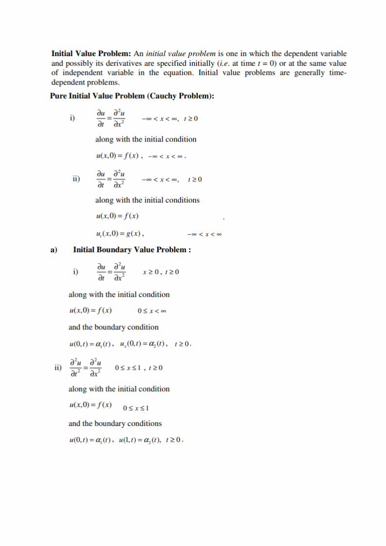
Boundary Conditions: The condition that the solution u assume given values on the

boundary of the region R.

Initial Conditions: When time t is one of the variables, u (or Ut = ∂u/ ∂t or both) may be

prescribed at t = 0

The order of a partial differential equation is the order of the highest order differential

coefficient occuring in the equation and the degree of the partial differential equation is the

degree of the highest order differential coefficient occurring in the equation.

Equation (1) is of Ist order I

st degree, equation (2) is of 2

nd order I

st degree whereas equation

(3) is of 2nd

order 3rd

degree.

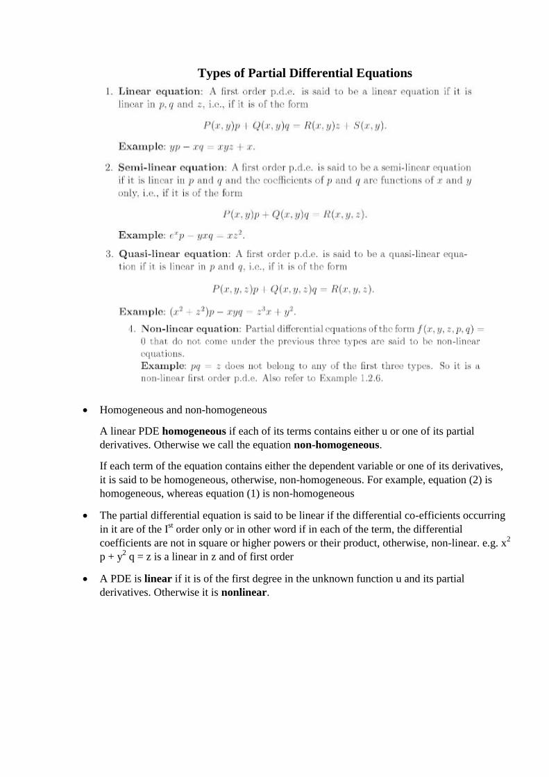
Types of Partial Differential Equations

Homogeneous and non-homogeneous

A linear PDE homogeneous if each of its terms contains either u or one of its partial

derivatives. Otherwise we call the equation non-homogeneous.

If each term of the equation contains either the dependent variable or one of its derivatives,

it is said to be homogeneous, otherwise, non-homogeneous. For example, equation (2) is

homogeneous, whereas equation (1) is non-homogeneous

The partial differential equation is said to be linear if the differential co-efficients occurring

in it are of the Ist order only or in other word if in each of the term, the differential

coefficients are not in square or higher powers or their product, otherwise, non-linear. e.g. x2

p + y2 q = z is a linear in z and of first order

A PDE is linear if it is of the first degree in the unknown function u and its partial

derivatives. Otherwise it is nonlinear.

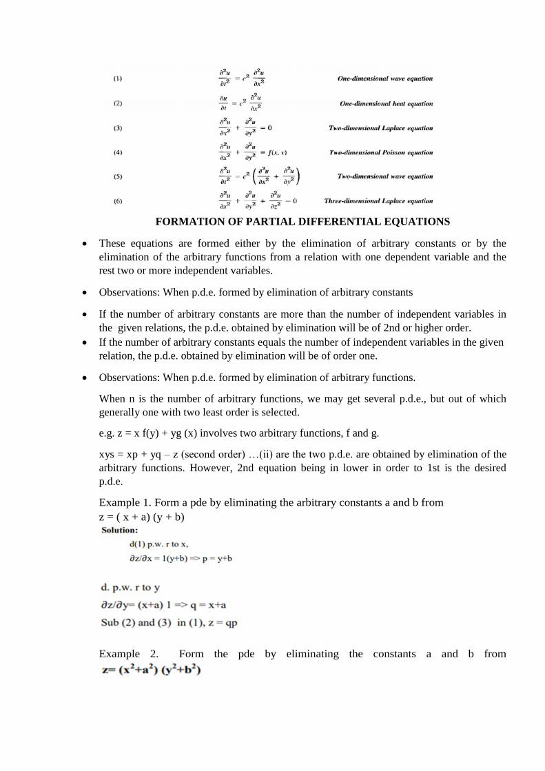
FORMATION OF PARTIAL DIFFERENTIAL EQUATIONS

These equations are formed either by the elimination of arbitrary constants or by the

elimination of the arbitrary functions from a relation with one dependent variable and the

rest two or more independent variables.

Observations: When p.d.e. formed by elimination of arbitrary constants

If the number of arbitrary constants are more than the number of independent variables in

the given relations, the p.d.e. obtained by elimination will be of 2nd or higher order.

If the number of arbitrary constants equals the number of independent variables in the given

relation, the p.d.e. obtained by elimination will be of order one.

Observations: When p.d.e. formed by elimination of arbitrary functions.

When n is the number of arbitrary functions, we may get several p.d.e., but out of which

generally one with two least order is selected.

e.g. z = x f(y) + yg (x) involves two arbitrary functions, f and g.

xys = xp + yq – z (second order) …(ii) are the two p.d.e. are obtained by elimination of the

arbitrary functions. However, 2nd equation being in lower in order to 1st is the desired

p.d.e.

Example 1. Form a pde by eliminating the arbitrary constants a and b from

z = ( x + a) (y + b)

Example 2. Form the pde by eliminating the constants a and b from

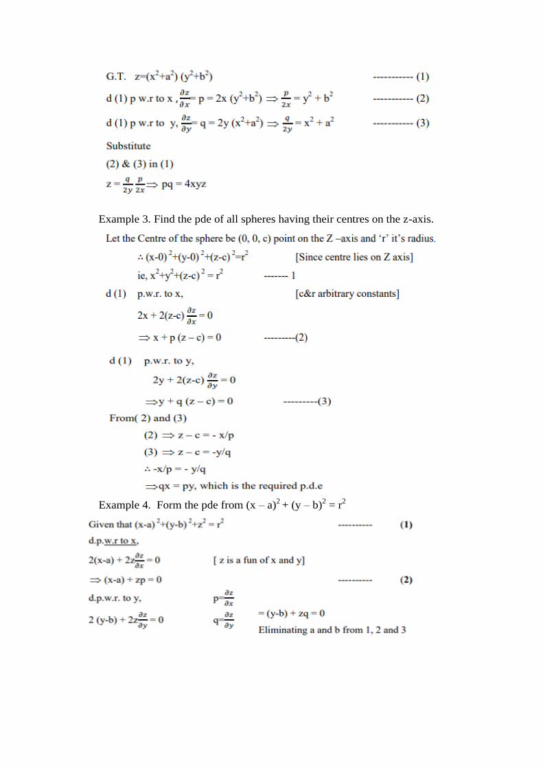
Example 3. Find the pde of all spheres having their centres on the z-axis.

Example 4. Form the pde from (x – a)

2 + (y – b)

2 = r

2

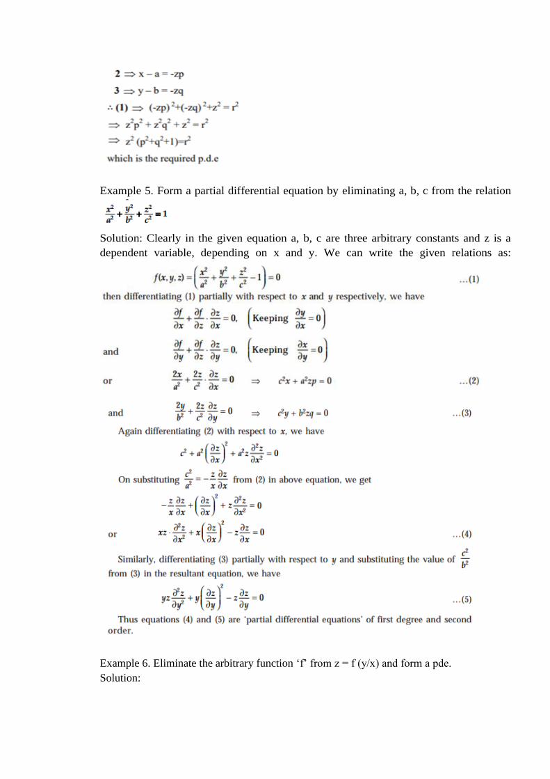
Example 5. Form a partial differential equation by eliminating a, b, c from the relation

Solution: Clearly in the given equation a, b, c are three arbitrary constants and z is a

dependent variable, depending on x and y. We can write the given relations as:

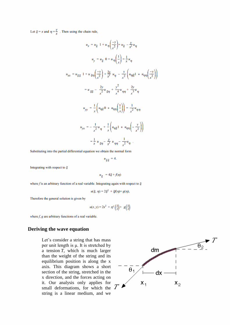
Example 6. Eliminate the arbitrary function ‘f’ from z = f (y/x) and form a pde.

Solution:

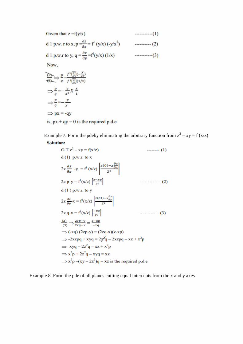
Example 7. Form the pdeby eliminating the arbitrary function from z2 – xy = f (x/z)

Example 8. Form the pde of all planes cutting equal intercepts from the x and y axes.

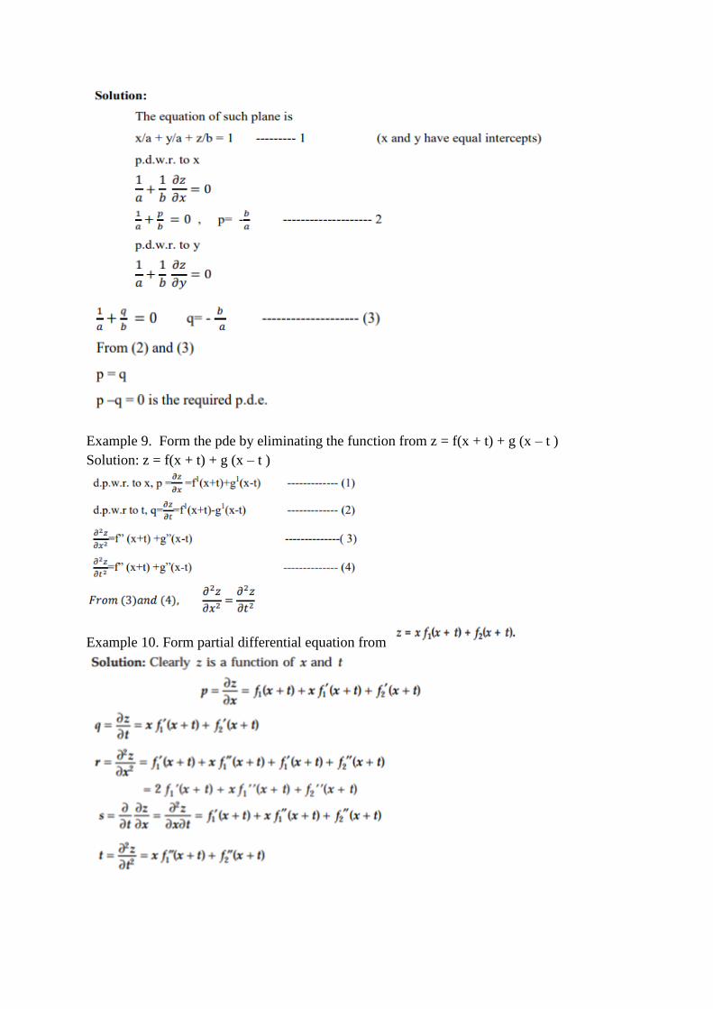
Example 9. Form the pde by eliminating the function from z = f(x + t) + g (x – t )

Solution: z = f(x + t) + g (x – t )

Example 10. Form partial differential equation from

COMPATIBLE SYSTEMS OF FIRST-ORDER PDEs

A system of two first-order PDEs f (x, y, u, p, q) = 0 (1) and g(x, y, u, p, q) = 0 (2) are said to be

compatible if they have a common solution

Equations (1) and (2) are compatible on a domain D if

(i) J = ∂(f ,g)/ ∂(p,q) = 0 on D.

(ii) p and q can be explicitly solved from (1) and (2) as p = φ(x, y, u) and q = ψ(x, y, u). Further, the

equation du = φ(x, y, u)dx + ψ(x, y, u)dy is integrable.

Theorem:

A necessary and sufficient condition for the integrability of the equation du = φ(x, y, u)dx + ψ(x, y,

u)dy is

[f , g] ≡ ∂(f , g) /∂(x, p) + ∂(f , g) /∂(y, q) + p ∂(f , g) /∂(u, p) + q ∂(f , g) /∂(u, q) = 0. ----(3)

equations (1) and (2) are compatible iff (3) holds

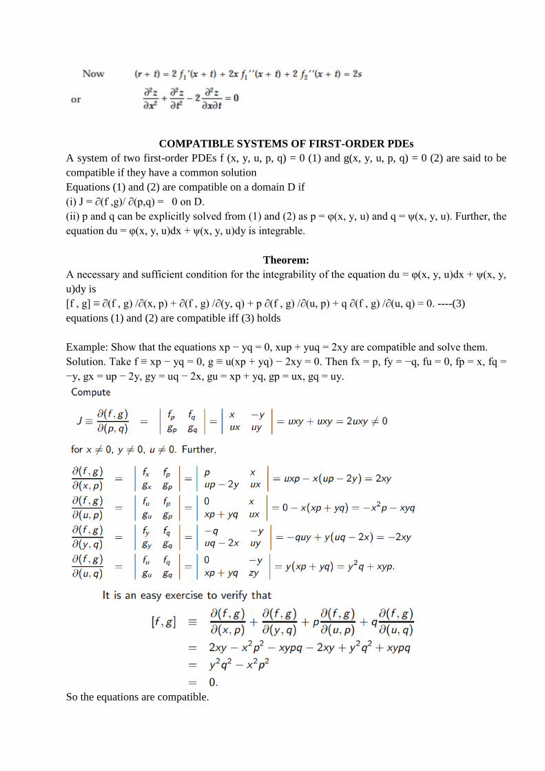
Example: Show that the equations xp − yq = 0, xup + yuq = 2xy are compatible and solve them.

Solution. Take f ≡ xp − yq = 0, g ≡ u(xp + yq) − 2xy = 0. Then fx = p, fy = −q, fu = 0, fp = x, fq =

−y, gx = up − 2y, gy = uq − 2x, gu = xp + yq, gp = ux, gq = uy.

So the equations are compatible.

Next step is to determine p and q from the two equations xp − yq = 0, u(xp + yq) = 2xy. Using

these two equations, we have uxp + uyq − 2xy = 0 =⇒ xp + yq = 2xy u =⇒ 2xp = 2xy u =⇒ p = y u

= φ(x, y, u). and xp − yq = 0 =⇒ q = xp y = xy yu =⇒ q = x u = ψ(x, y, u).

Substituting p and q in du = pdx + qdy, we get udu = ydx + xdy = d(xy), and hence integrating, we

obtain u 2 = 2xy + k, where k is a constant.

CHARPIT’S METHOD

It is a general method for finding the general solution of a nonlinear PDE of first-order of the form f

(x, y, u, p, q) = 0.

Basic Idea: To introduce another partial differential equation of the first order g(x, y, u, p, q, a) = 0

which contains an arbitrary constant a and is such that

(i) equations can be solved for p and q to obtain p = p(x, y, u, a), q = q(x, y, u, a).

(ii) The equation du = p(x, y, u, a)dx + q(x, y, u, a)dy is integrable.

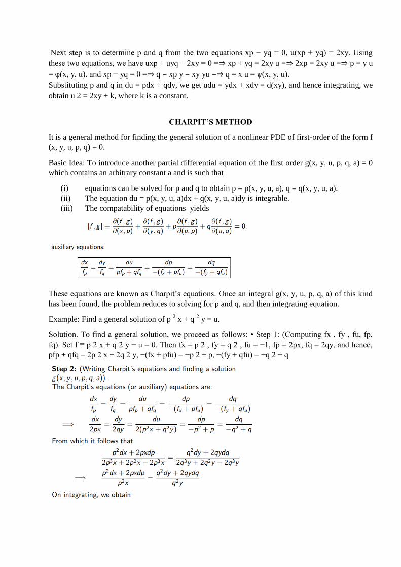
(iii) The compatability of equations yields

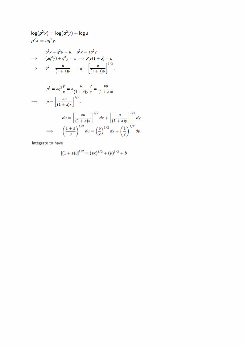
These equations are known as Charpit’s equations. Once an integral g(x, y, u, p, q, a) of this kind

has been found, the problem reduces to solving for p and q, and then integrating equation.

Example: Find a general solution of p 2 x + q

2 y = u.

Solution. To find a general solution, we proceed as follows: • Step 1: (Computing fx , fy , fu, fp,

fq). Set f ≡ p 2 x + q 2 y − u = 0. Then fx = p 2 , fy = q 2 , fu = −1, fp = 2px, fq = 2qy, and hence,

pfp + qfq = 2p 2 x + 2q 2 y, −(fx + pfu) = −p 2 + p, −(fy + qfu) = −q 2 + q



UNIT –II – CURVES AND SURFACES,FIRST ORDER PDE – SMT5204

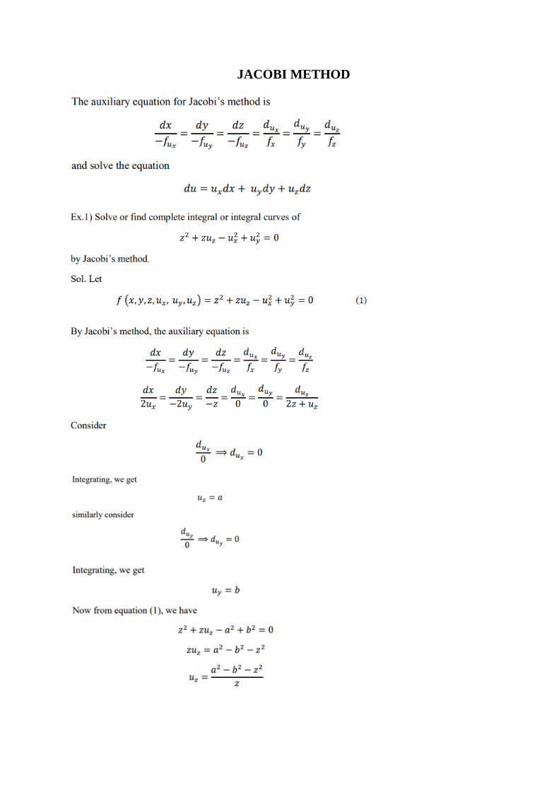
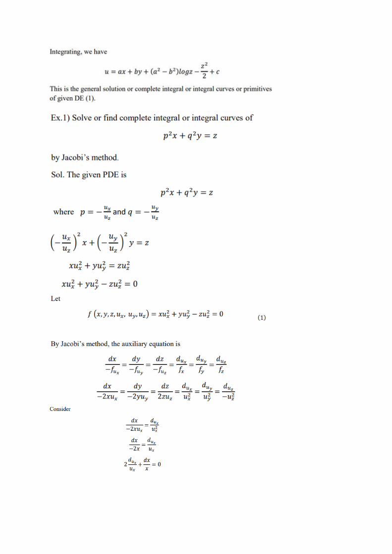
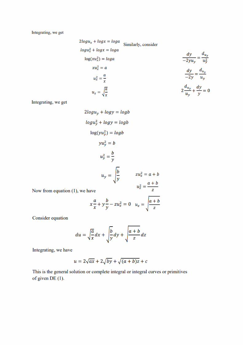
JACOBI METHOD

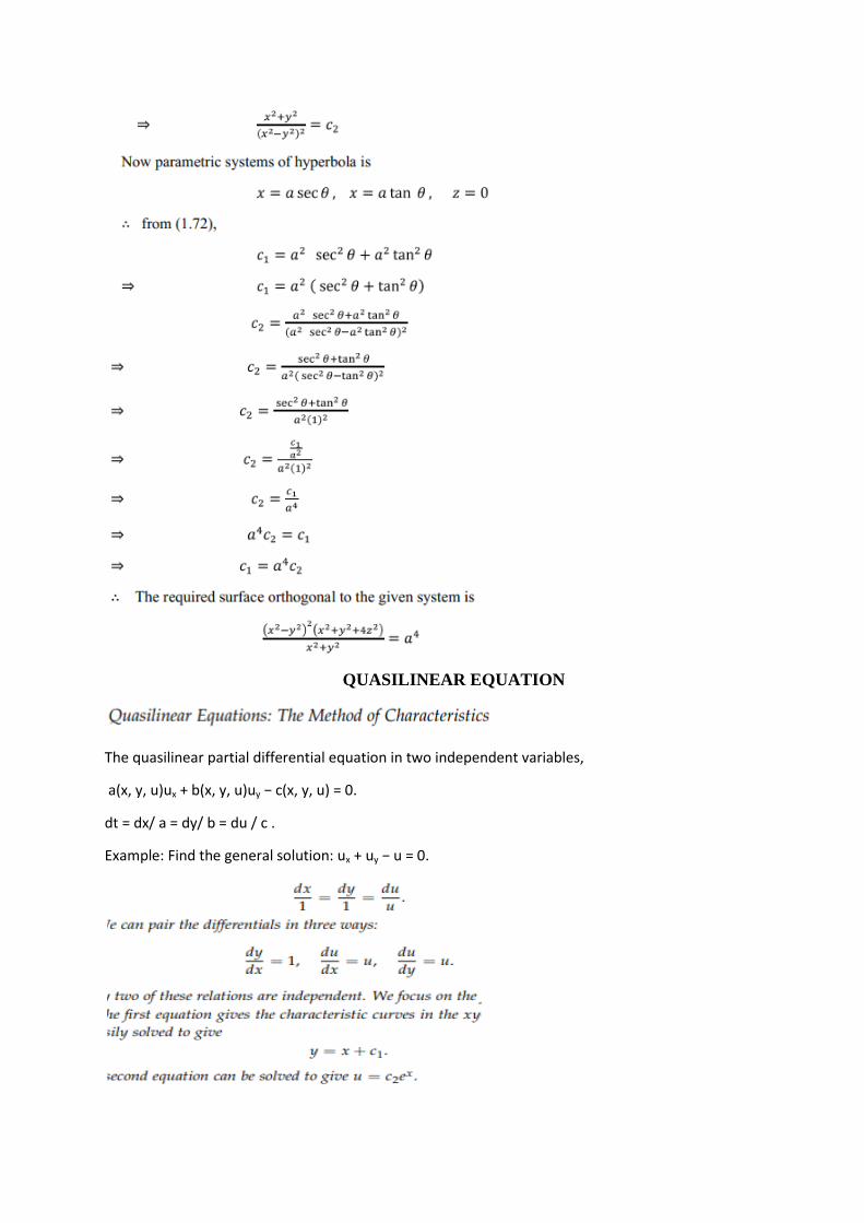
QUASILINEAR EQUATION

The quasilinear partial differential equation in two independent variables,

a(x, y, u)ux + b(x, y, u)uy − c(x, y, u) = 0.

dt = dx/ a = dy/ b = du / c .

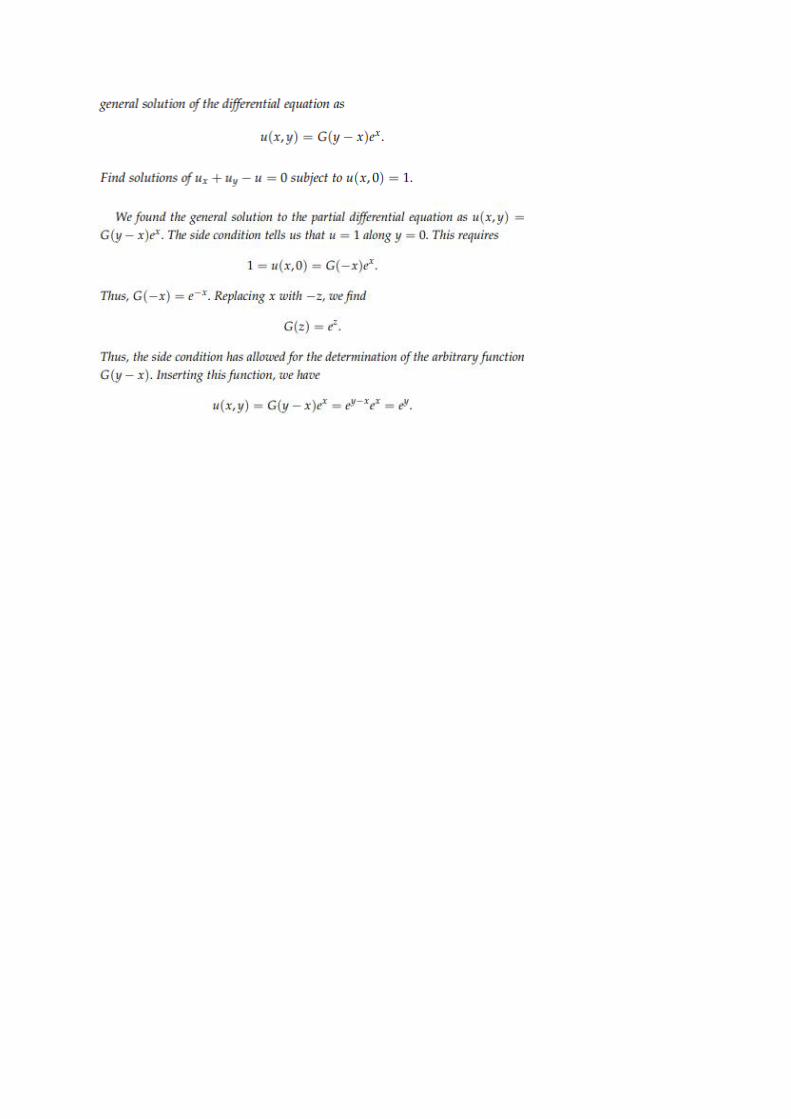
Example: Find the general solution: ux + uy − u = 0.



UNIT –III – SECOND ORDER PDE – SMT5204

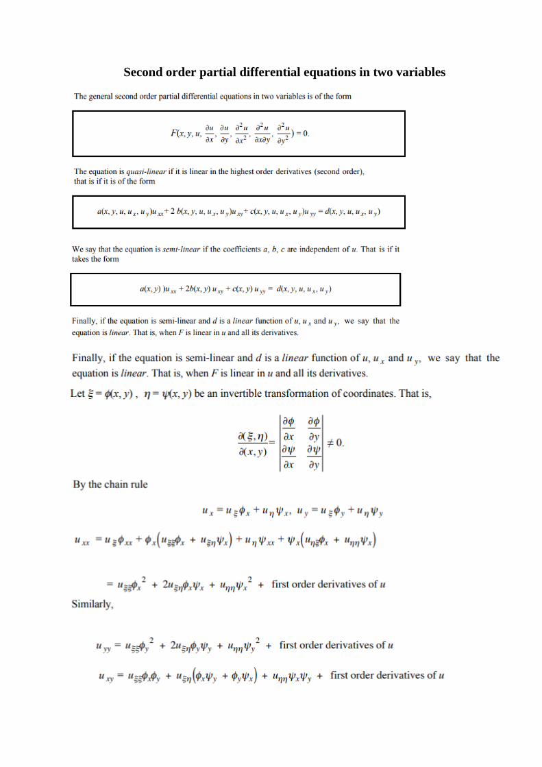
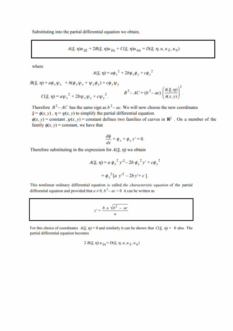
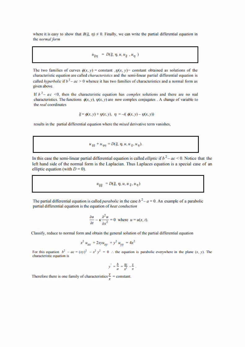
Second order partial differential equations in two variables

Deriving the wave equation

Let’s consider a string that has mass

per unit length is μ. It is stretched by

a tension T, which is much larger

than the weight of the string and its

equilibrium position is along the x

axis. This diagram shows a short

section of the string, stretched in the

x direction, and the forces acting on

it. Our analysis only applies for

small deformations, for which the

string is a linear medium, and we

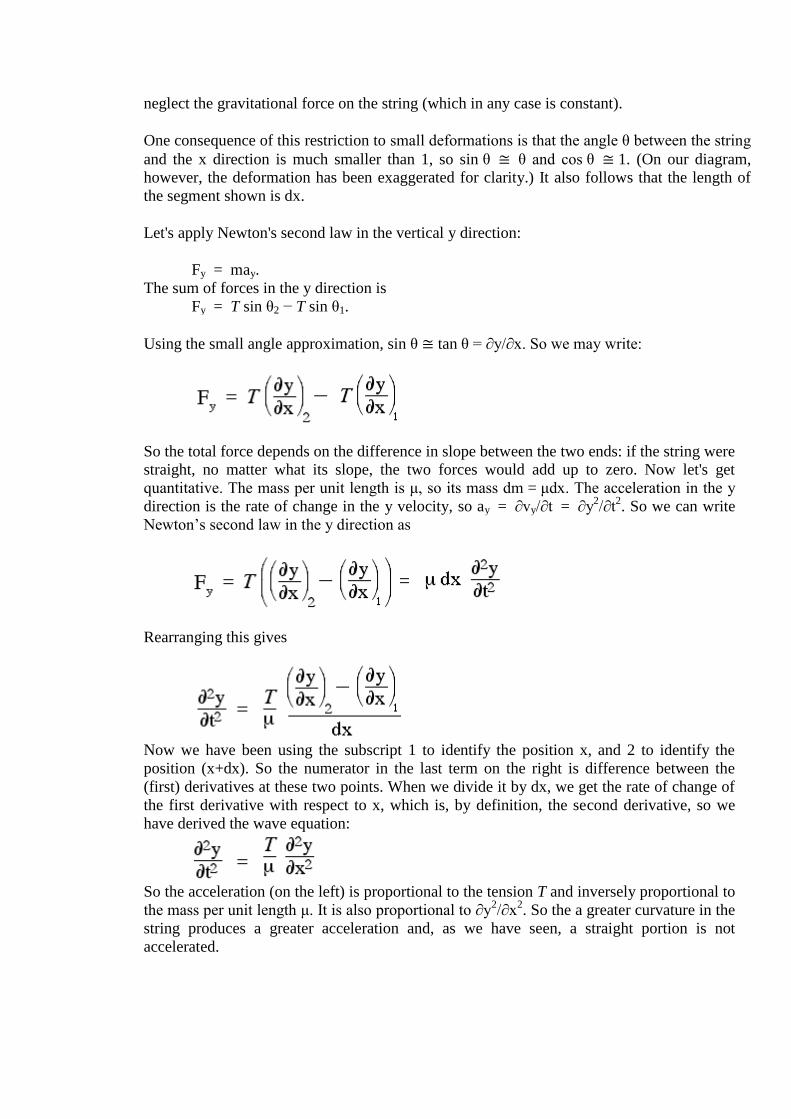
neglect the gravitational force on the string (which in any case is constant).

One consequence of this restriction to small deformations is that the angle θ between the string

and the x direction is much smaller than 1, so sin θ ≅ θ and cos θ ≅ 1. (On our diagram,

however, the deformation has been exaggerated for clarity.) It also follows that the length of

the segment shown is dx.

Let's apply Newton's second law in the vertical y direction:

Fy = may.

The sum of forces in the y direction is

Fy = T sin θ2 − T sin θ1.

Using the small angle approximation, sin θ ≅ tan θ = ∂y/∂x. So we may write:

So the total force depends on the difference in slope between the two ends: if the string were

straight, no matter what its slope, the two forces would add up to zero. Now let's get

quantitative. The mass per unit length is μ, so its mass dm = μdx. The acceleration in the y

direction is the rate of change in the y velocity, so ay = ∂vy/∂t = ∂y2/∂t

2. So we can write

Newton’s second law in the y direction as

Rearranging this gives

Now we have been using the subscript 1 to identify the position x, and 2 to identify the

position (x+dx). So the numerator in the last term on the right is difference between the

(first) derivatives at these two points. When we divide it by dx, we get the rate of change of

the first derivative with respect to x, which is, by definition, the second derivative, so we

have derived the wave equation:

So the acceleration (on the left) is proportional to the tension T and inversely proportional to

the mass per unit length μ. It is also proportional to ∂y2/∂x

2. So the a greater curvature in the

string produces a greater acceleration and, as we have seen, a straight portion is not

accelerated.

A solution to the wave equation

The wave equation is a partial differential equation. Sine waves can propagate in a one

dimensional medium like a string. And we know that any function f(x − vt) is a wave

travelling at speed v. In the first chapter on travelling waves, we saw that an elegant version

of the general expression for a sine wave travelling in the positive x direction is

y = A sin (kx − ωt + φ). A suitable choice of x or t axis allows us to set φ to zero, so let's

look at the equation

y = A sin (kx − ωt)

to see whether and when this is a solution to the wave equation

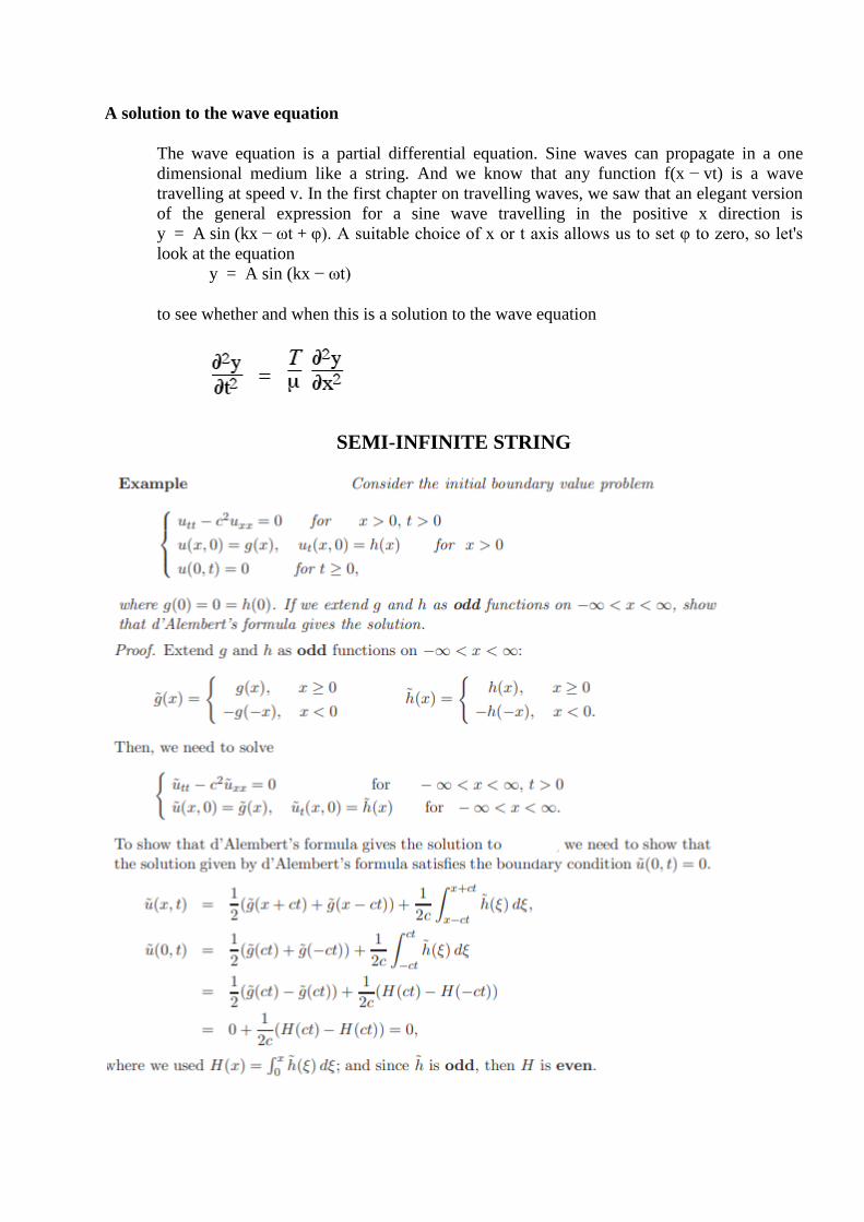
SEMI-INFINITE STRING



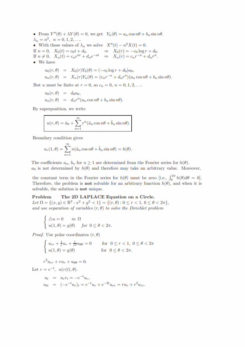
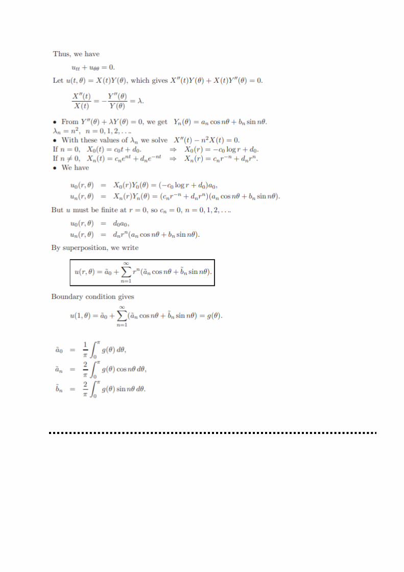
UNIT – IV – BOUNDARY VALUE PROBLEMS – SMT5204

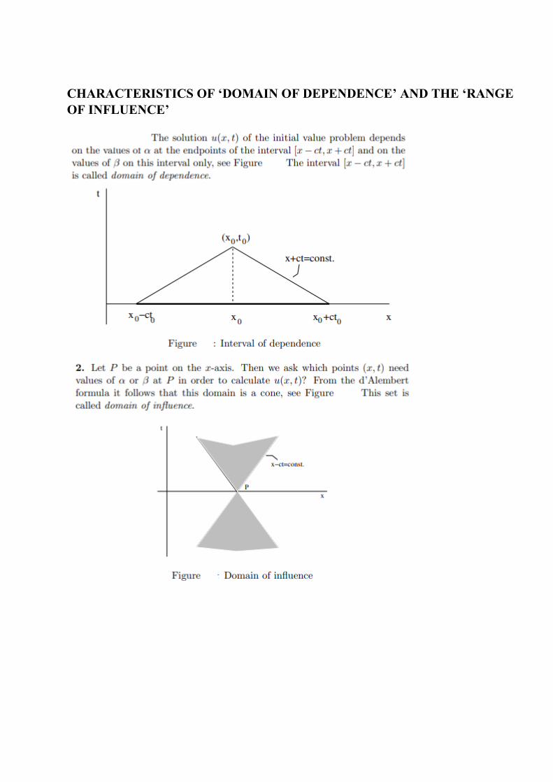
CHARACTERISTICS OF ‘DOMAIN OF DEPENDENCE’ AND THE ‘RANGE

OF INFLUENCE’

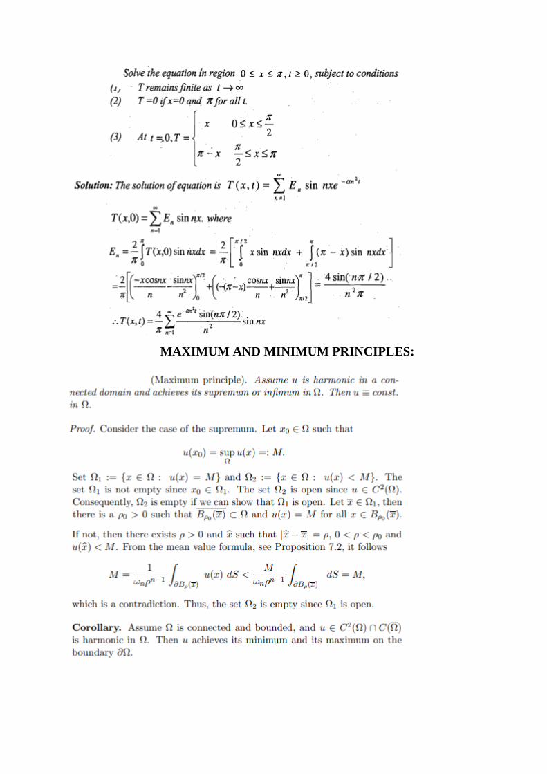
MAXIMUM AND MINIMUM PRINCIPLES:



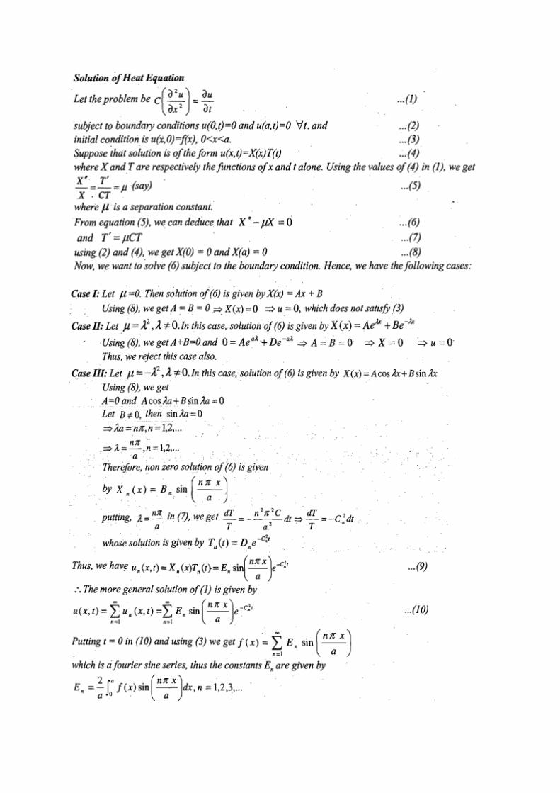
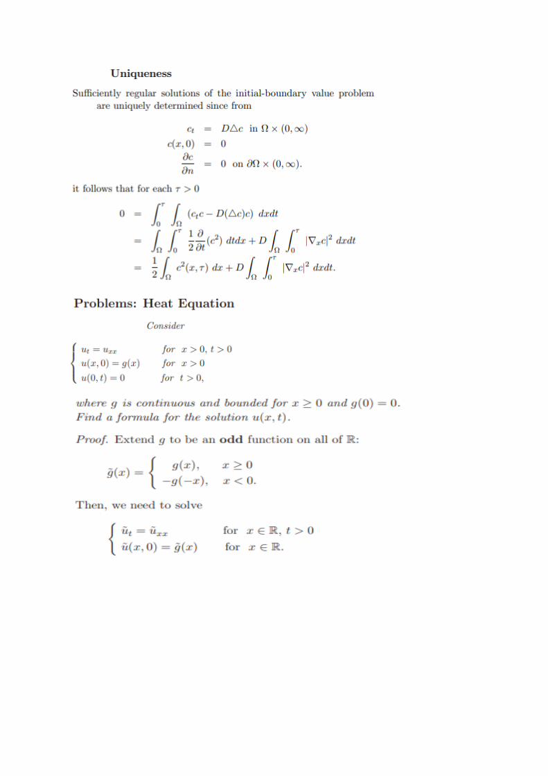
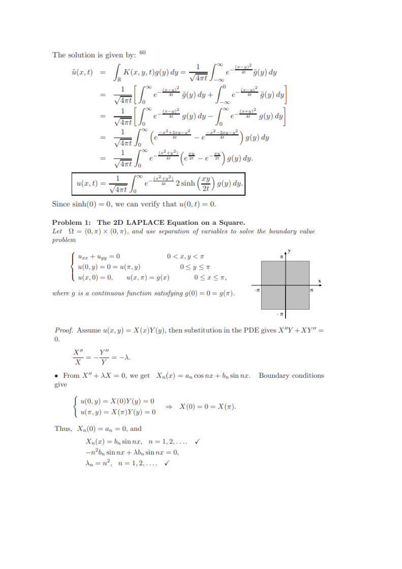
UNIT – V – DIRICHLET AND HEAT PROBLEM – SMT5204

school of science and humanities department of mathematics

Documents