School Choice, Student Sorting and AcademicPerformance†

Andrei Munteanu§

September 20, 2021

AbstractIn this paper, I first study the effects of school choice on student sorting patterns andacademic performance. Second, I explore possible channels through which sorting impactsperformance. The main finding is that school choice greatly increases the dispersion in testscores rather than acting as a “tide that lifts all boats”. The setup I study is Romanianhigh schools, where students compete for seats based on national standardized exams. Iscrape and construct a novel dataset matching twelve years and more than two millionstudent admission and graduation records, teacher hiring records and school spendingrecords. I first show that having more schools to choose from increases student sorting. Ifind that across towns of similar sizes, whenever there are more schools to choose from,student sorting by ability across schools is more pronounced. Second, using this variation inschool numbers across similar locations, I show that increases in student sorting causallybenefit high-scoring students and hinder low-scoring students, thus increasing outcomeinequalities. I confirm these findings by focusing on high school openings in small towns.Openings lead to increases in student sorting across schools and result in higher score gapsbetween high- and low-ability students. Lastly, I use teacher and expenditure data to showthat observed effects on student scores can mainly be attributed differences in teachersacross schools (48%), compared to peer effects (25%) and school spending (5%). My resultsuggest that increased school choice leads to a polarization in student outcomes that isdriven by high-scoring students sorting into schools with better teachers and better peers.

JEL Classification : I21, I24, H52Keywords: education, sorting, inequality, peers, teachers

†A previous version of this paper circulated under the title “Student Sorting and Academic Performance”.§Center for Economic and Social Research, University of Southern California. email: amuntean@usc.edu.

I am deeply indebted to Fabian Lange, Francesco Amodio and Nicolas Gendron-Carrier for excellent supervi-sion and advice, as well as Christopher Barrington-Leigh, Rui Castro, Ana-Maria Dimand, Rohan Dutta, JohnGalbraith, Andra Hiriscau, John Klopfer, Laura Lasio, Daniela Morar, Markus Poschke, Fernando Saltiel, XianZhang and all the seminar participants and organizers at McGill University, Goethe University, UQAM, Univer-sity of Pittsburgh, GEEZ, Nederlandse Economenweek 2020 and the E-conomics of Education Graduate StudentWorkshop. I am also indebted to Andreea Mitrut, Gabriel Kreindler, Cristian Pop-Eleches and Diana Comanfor help on obtaining the data used for this study. All errors are my own.

1 Introduction

In this paper, I attempt to shed light on the claim that school choice can act as a “rising

tide that lifts all boats” (e.g. Hoxby (2007)). The implication is that expanding school choice

would exert competitive pressures on schools, forcing them to improve their service or risk losing

students. In the United States in particular, where student literacy and numeracy levels have

stagnated for the past decades, school choice has often been presented as a panacea. However,

the system-wide implications of school choice have been difficult to prove, especially since a very

small proportion of students attend schools operating under school choice and these schools tend

to be high-quality, selective schools.

In this paper, I first study the link between school choice, student sorting patterns and

subsequent student performance, in the context of Romanian high schools. Unlike in the US,

Romanian high school admissions are fully based on school choice. Students compete for seats

in schools across the country based on standardized exam scores. This allows me to study the

system-wide implications of school choice. To this end, I put together a dataset covering the

universe of Romanian high school students across 11 years (2004-2015 entering cohorts). These

data consist of more than two million students originating from more than 10,000 middle schools

and attending close to 1,500 high schools across more than 500 towns. I augment these data by

adding detailed geographic information on the location of the middle and high schools.

Second, I explore the underlying channels through which school choice ultimately affects

student performance. I match the student admission and graduation records to novel, web

scraped data on the universe of teacher hires over five years. These data include teacher exam

scores on subject-specific exams used to allocate them to teaching jobs and education, experience

and GPA information and cover close to 200,000 teacher exam scores and in excess of 40,000

teacher hires. I build a dataset containing all high school expenditures on goods and services for

more than ten years, totaling more than a million transactions. I thus have unique data, rich

in information on students, locations, inputs, and teachers that I leverage to study sorting on

ability, its effects on academic performance, and the mechanisms through which sorting affects

academic performance.

1

The causal effect of student sorting on academic performance is difficult to identify because

school choices are endogenous. I overcome this issue in two ways. First, I exploit mechanically-

arising variation in sorting patterns induced by differences in high school numbers across towns

of similar sizes. In Romania, a national entrance exam determines high school admissions.

High-scoring students have priority over low-scoring ones when it comes to high school choices.

Students can then sort across high schools along entrance grades at will. As a result, student

sorting levels are high across the country. Moreover, this setup induces differences in sorting

patterns across towns with similar populations but different numbers of high schools. For

example, a high entrance grade student in a town with two high schools can sort into a much

more selective high school than their counterpart in a similar-sized town with only one high

school. By interacting student entrance scores with number of high schools in their towns, I

construct an instrument that shifts the type of high school students attend. This allows me to

compare graduation scores of similar-ability students across otherwise comparable towns that

differ only in the number of high schools to identify the effects of sorting.

Second, I use new high school openings in towns with few high schools in a triple difference

framework. The data’s panel nature allows me to key in specifically on school openings, which

disrupt preexisting sorting patterns. A new school opening disrupts sorting patterns at the local

level. More specifically, I measure how a school opening differentially affects high-ability and

low-ability students by comparing them to their counterparts in similarly-sized towns where

there are no new schools opening.

Lastly, I disentangle the channels through which sorting affects academic performance. The

rich data in the Romanian setup allow me to speak to three possible channels: peer effects,

differences in teacher ability and school expenditure. Leveraging differences in peer entrance

scores across cohorts within the same high schools and differences in teacher examination grades

and per-student school expenditures across high schools, I measure these three channels’ relative

contribution toward student performance.

I contribute directly to the literature on student tracking and sorting, which has mixed

findings. While some studies find that tracking or school choice increase dispersion of outcomes

2

between high- and low-ability students,1 others find that tracking can benefit both low-ability

students and high-ability ones.2 One reason behind these mixed finding is the fact that student

sorting and its effects on learning are very context-specific. For example, in terms of peers

and access to high-ability teachers and other learning resources, student sorting in rural sub-

Saharan Africa, where students of very different ages and abilities are often pooled into one

classroom, has very different implications than in large urban areas in the Unites States, where

sorting often leads to unequal access to teaching resources. Thus, studying the channels through

which sorting impact performance and their relative importance is crucial if we are to gain any

understanding about the ways in which sorting affects student outcomes.

My main results follow. Student sorting along ability is more prevalent in towns with more

high schools, even after controlling for student population. The largest jump in sorting occurs

between towns with one high school, in which no sorting at the school level is possible, and

comparable towns with two high schools. This suggests that the number of schools is the main

driver of student sorting.

The instrumental variable approach suggests that conditional on student entrance score,

attending a high school with a 1 percentile higher average entrance score increases a student’s

graduation score by 0.16 percentiles. This has two implications on graduation scores. First,

increasing sorting levels are accountable for widening graduation score gaps between high- and

low-ability students within towns. Thus, this gap is larger in many-high school towns, which

experience high degrees of sorting. More specifically, in locations with more than 15 high schools,

the high levels of sorting at the school levels lead to a 12 percentile widening of the performance

gap between top entrance score decile students and their counterparts in the lowest decile. In

towns with only one high school, this figure shrinks to 3 percentiles.

Additionally, sorting widens the performance gap between urban high-ability students (who

can attend selective schools) and rural high-ability students (who cannot). The gap between

low-ability urban students (who attend the worst urban schools) and low-ability rural students

(who benefit from low sorting in rural areas) shrinks via sorting. Sorting at the school levels1Hanushek and Wößmann (2006), Malamud and Pop-Eleches (2011), Imberman (2011), Pop-Eleches andUrquiola (2013), Chmielewski (2014) and Jakubowski et al. (2016)

2Figlio and Page (2002), Duflo et al. (2011) and Collins and Gan (2013).

3

is responsible for a 4 percentile widening of the graduation score gap between top entrance

grade decile students in cities and their counterparts who attend school towns with only one

high school. At the other end of the distribution, sorting causes low entrance score students in

cities to underperform compared to their counterparts in one high school towns by 4 percentiles.

These findings are persistent even when controlling for town fixed effects, student populations

across locations and interactions between student populations and entrance scores. Thus, the

results are not driven by differences in town sizes. There is a strong sense that, conditional on

town size and own entrance score, the number of high schools in a location directly impacts

student scores via sorting.

The results generated from school openings confirm these findings: the opening of a new

school disproportionately benefits high-ability students who can self-select into the best school,

while low-ability students become increasingly segregated into worse schools. A school’s opening

in a small town leads to a 4 to 10 percentile widening of the graduation gap between top entrance

score quartile students and their counterparts in the lowest quartile, compared to similar towns

without new school openings. Moreover, there is evidence that a school opening lowers average

graduation scores in a town, conditional on student entrance grades.

I proceed to a decomposition of the channels through which sorting into a better school

impacts grades. Overall, the three channels I study (peer effects, teacher ability and school

expenditures) explain roughly 78% of the effect of attending a better high school. Differences

in teacher ability and peer effects each explain 48% and 25% of the total effects of attending a

better high school, while differences in school spending only explain 5% of the total effect.

I conduct several robustness checks. First, I adjust for students dropping out of high school

(or out of my data) using a Heckman correction. I then address the potentially endogenous

migration of students between towns by defining local education markets endogenously. I use

them as the unit of analysis instead of towns. Lastly, my models allow similar entrance grade

students from towns (or markets) with different populations to perform differently on the grad-

uation exam. This captures the fact that similar-ability students in towns of different sizes

face potentially different levels of income, socioeconomic inequality, parent education, etc. The

4

results are robust to all these different specifications.

As a secondary set of results, I explore how student sorting correlates with teacher sorting,

school expenditures, and student achievement at graduation. This sheds light on the possible

channels through which sorting impacts student achievement. The analysis delivers four sets of

results.

First, using data from teacher examinations used to assign teachers to teaching jobs, I find

that teacher sorting patterns mirror those of students: high-ability teachers sort into schools

with high-ability students. Moreover, conditional on ability, students in schools with better

teachers score higher on the graduation exam. On average, a one percentile point higher grade

on teacher examinations is associated to a 0.08 increase in student graduation score on that

subject, conditional on student ability. This estimate is likely a lower bound, as the data do not

allow for student-teacher matching at the classroom level, only at the school level and teacher

data contain only newly-hired teachers, excluding teachers who were already employed. Lastly,

there are complementarities between student and teacher abilities: high-ability students benefit

from high-ability teachers more than low-ability students.

Second, using year to year quasi-random variation in the abilities of entering cohorts within a

school to identify potential peer effects. While, on average, peer effects are not significant, there

is evidence that this effect is heterogeneous in students’ ranking within their track. Higher

ability students within their tracks or schools benefit more from increases in peer admission

scores. A one percentile increase in average peer entrance score at the school level increases

top student graduation grades by 0.17 percentiles on average. Lowest entrance score students’

graduation grades are negatively impacted, with a magnitude of 0.10.3

Third, there is no evidence that school spending on goods and services improves student

scores. Although low-admission score students in Romania attends schools with higher levels

of per-student spending, both nationally and within towns, this does not translate into higher

scores at graduation, conditional on admission scores and teacher ability.

Several policy implications follow from this analysis. First of all, policies that increase3This is consistent with so-called “single crossing” peer effects models. See Sacerdote (2011) for more details.This is also consistent with survey evidence by Pop-Eleches and Urquiola (2013), who document higher instancesof bullying aimed at low-ability students within Romanian high schools, leading to marginalization.

5

student segregation on ability (for example, school choice policies or tracking) exacerbate per-

formance gaps between high- and low-achieving students and between top urban and top rural

students. In particular, low-ability students in urban areas emerge as the most negatively af-

fected group by sorting and school choice. On the bright side, my results suggest that the

exacerbation of inequalities caused by student sorting can be mitigated by incentivizing high-

ability teachers to work in low-ranking schools. However, this may be socially wasteful, as

there is evidence that high-ability students disproportionately benefit from being taught by

high-ability teachers. Thus, reallocating top teachers to bad schools may not be a particularly

efficient allocation of teaching resources.

Second, school openings, especially when there is significant school choice, may not bene-

fit students equally. The findings suggest that school openings, in particular in small towns,

disproportionately benefit high-ability students. These students benefit from the increase in

school-level sorting following the opening of a new school. After the opening, they are sepa-

rated from their low-ability counterparts, who are segregated into low-quality schools. Thus,

policymakers have to be very mindful of sorting effects when opening a new school and how this

can be detrimental to low-ability students.

This paper contributes to the literature in two ways. First of all, it speaks directly to the

literature on student tracking and student sorting. The main challenge in this literature is

addressing the endogeneity of school choices. Indeed, student enrollment in schools may be

correlated with unobserved individual, family or location characteristics.4 To address this issue,

authors use quasi-experimental shifters of school choice. For example, some studies use busing

or lotteries of low-income students to high-income schools or variations in student assignments

to schools.5 While these designs are useful in pinpointing the effects of attending better schools

for students benefiting from these policies, they do not speak to the effects of sorting on the

entire population of students.

In this paper, I introduce a new instrument that shifts local student sorting patterns. Indeed,

4Such as motivation, parental involvement or distance to school.5For example, Dobbie and Fryer Jr (2011) exploit a Harlem lottery system, Angrist et al. (2012) exploit asimilar Massachusetts system, Banerjee et al. (2007) study an experimental intervention in India and Chettyet al. (2011) use random assignment to kindergarten classes from Project STAR.

6

in the Romanian high school system, the number of schools in an educational market affects the

type of schools students attend, conditional on ability for the entire distribution of students.

This enables me to causally estimate the effects of sorting on the entire student population. I

provide credible evidence that increases in sorting exacerbate educational inequalities.

Second, the student-teacher-school spending dataset I build allows me to investigate the

effects of peers, teachers and school resources on educational outcomes. Most importantly, this

setup allows me to measure the relative contribution of these channels towards educational

achievement. To the best of my knowledge, this is the first paper that succeeds in disentangling

these channels. In particular, the finding that teacher ability is of much greater consequence

than peer effects is new and has important policy implications.

In terms of peer effects, Chetty et al. (2011), Sacerdote (2001), Sacerdote (2011) and recently

Patacchini et al. (2017) and Carrell et al. (2018) find significant, but typically small, peer effects

on student outcomes. However, other studies, including Burke and Sass (2013) find little in

the way of economically meaningful peer effects and highlight. Angrist (2014) also identifies

potential identification issues that put into question some of the literature’s findings. My own

results suggest that peer effects are not significant for the average student. However, this masks

significant heterogeneity, as relatively high-ability students benefit from better peers, while

low-ability students do not.

I also contribute to the study of teacher value-added. It is found to be the main driver

of student achievement differences, conditional on student ability, in several papers.6 The

effects of teacher ability on student achievement are obfuscated, however, by poor measures

of teacher ability. In particular, teacher’s education or experience does not seem to correlate

with teacher value-added.7 In practice, many studies avoid this issue by directly measuring

teacher value-added by observing teachers who switch schools or classrooms.8 Unfortunately,

this identification strategy is plagued by the issue that teacher mobility and student school

choice are most likely non-random, particularly along unobserved dimensions. The Romanian

6For example Rockoff (2004), Hanushek et al. (2005), Chetty et al. (2014), Petek and Pope (2016) and andJackson (2018).

7For example, Dobbie and Fryer Jr (2013).8For example, Rivkin et al. (2005).

7

data provide very rich measures of teacher ability, which allows me to directly measure teaching

skills without having to resort to teacher mobility.9 In line with the literature, I find that

teacher ability is the main channel through which attending a better school impacts educational

achievement.

To summarize, using very rich data on student admission and graduation records, teacher hir-

ing and school expenditures, I analyze how student sorting affects academic performance. I find

that students sort more along entrance grades in locations with more high schools, even when

controlling for town population. Using the variation in sorting patterns induced by differences

in high school numbers across similar-sized towns, I find that increases in sorting exacerbate

educational outcome inequalities between high- and low-ability students. An analysis of high

school openings confirms these findings: when a new high school opens in a small town, student

sorting becomes more pronounced and the graduation score gap increases. Lastly, roughly half

of the observed effects of sorting on grades can be attributed to differences in teacher ability,

compared to one quarter for peer effects and a mere 5% for school expenditures.

The remainder of this paper is structured as follows. Section 2 describes the Romanian high

school system and all the data sources used. Section 3 highlights student sorting and student

achievement gaps prevalent in the data that serve as a motivation for the paper. Section

4 lays out the primary identification strategy and causal results linking student sorting and

achievement. Section 5 analyzes the possible channels through which sorting likely impacts

student scores. Lastly, section 6 provides a discussion and conclusion.

2 Setup and Data

2.1 Institutional Framework

The Romanian high school allocation system is unique and very useful for studying the conse-

quences of school choice. In other setups, such as the US, only a limited number of jursidictions

and schools allow school choice, typically in parallel to large traditional public and private school

9Mainly from a subject-specific exam used to assign teachers to jobs, with high scoring teachers having priorityover low scoring ones. Additionally, teacher undergraduate GPA, education level and another set of exam usedby teachers to advance in rank (advances in rank come with a salary increase) are also available.

8

systems. Even then, school choice is constrained by a number of geographic, family and/or so-

cioeconomic and demographic conditions, or students are simply selected by schools on case

by case basis. For example, charter schools, even those serving underprivilegd children, may

select students and their families based on interviews, thus cherrypicking the best students and

maintaining high attrition rates in order to keep only the highest-performing students. Even

in the Boston public school mechanism, where students are assigned to schools via a lottery,

distance to school is a criterion used to assign students to schools. The fragmented nature

of these markets, their coexsitence with other, more tradiaitonal, school alternatives and the

complicated selection of students into schools make it difficult, if not impossible, to asses the

impact of school choice, especially across the ability distribution.

In contrast, as will be described shortly, the Romanian high school system offers an uncon-

strained, transparent and centralized allocation mechanism in which school choice is absolute.

Moreover, since public high schools account for more than 98% of enrolment,10 there are no

concerns of selection into the school choice system and it allows the study of the consequences

of school choice across the entire distribution of students. In addition, even though all schools

in this setup are public, they face considerable competitive pressures to attract better students

and teachers, as schools at the bottom end of the distribution that cannot fill their available

seats or cannot attract teachers face pressures to merge with other schools or close down en-

tirely. Therefore, this setup is useful for studying the competitive pressures that proponents of

school choice argue can improve the eduactional system not unlike a “rising tide that lifts all

boats”.

In the next paragraphs, I describe how the Romanian high school admission system works

and how it presents a perfect setup to study school choice, uncontaminated by the issues high-

lighted previously. I was able to scrape and build a dataset of more than two million matched

student admission and graduation records and match it, for the first time, to close to 40,000

scraped teacher evaluation and hiring records and to more than a million school purchases of

goods and services. These allow me to explore the ways in which school choice impacts student

101.7% of high school students attended a private school in the 2017-2018 school year, according to the RomanianNational Institute of Statistics.

9

sorting, what the impact of sorting is on student outcomes and how unequl access to teachers

and resources impact the effects of school choice on students in different parts of the test score

distribution.

2.1.1 High School Admissions and School Choice

Each year, Romanian middle school graduates are assigned to high schools based on a unique

centralized mechanism. Each student receives an admission score. This score is based on two

components: first, their middle school (grades 5-8) GPA and, second, a score on a national,

standardized high school admission exam covering different subjects (mathematics, Romanian,

and a choice of history or geography). The admission score places different weight on the two

components in different years, but at least half of the score is attributed to the admission exam.

After writing the exam and receiving their admission scores, students fill out a list of ranked

preferences over combinations of high schools and tracks they wish to attend. Tracks include,

but are not limited to: mathematics and computer science, literature, natural sciences, social

sciences and many technical or service tracks. For example, a student can rank the literature

track in high school A as their first choice, the literature track in high school B as their second

choice and the science track in high school A as their third choice. Students can choose more than

a hundred preferences if they so desire, so preference truncation is not an issue. Moreover, there

is no geographic restriction constraining which high schools students can express preferences

over.

Students are then allocated to high schools based on a centralized algorithm. After all

students submit their preference lists, they are ranked in descending order of their admission

scores. Then, starting with the top-ranked student, students are assigned to their most preferred

high school track that still has vacant seats. There are no other geographic, socioeconomic or

family criteria that is used to assign students to schools. This mechanism ensures, first, that

high-scoring students have absolute priority over lower-etrance score students and, second, that

students have no incentive to strategically manipulate their preferences over tracks in hope of

a better assignment.11

11In other words, the mechanism, which is equivalent to a serial dictatorship, is incentive compatible.

10

2.1.2 High School Graduation Exam

After completing four years of high school (grades 9-12), Romanian high school students register

to take a national, standaridized high school exit exam. This exam consists of several subjects,

including Romanian, mathematics, as well as other track-specific subjects. Receiving a high

school diploma is contingent on passing this exam (obtaining a grade of at least 50% on all

components). Morevoer, for students planning to attend postsecondary schooling, the exit

exam grade exam can be used as an admission requirement. This exam is thus high stakes

and is useful in comparing student abilities at high school graduation. I match the high school

graduation exam data to the high school admission data to obtain more than two million student

records.12

2.1.3 Teacher Allocation

Each year, teachers are assigned to high school teaching jobs in a way that mirrors the way

students are assigned to high school seats. In order to apply for teaching jobs, prospective

teachers must pass a yearly, standardized subject-specific examination that has an oral and a

written component. Although the teacher allocation mechanism is slightly more complicated

than the student one,13 high-scoring teachers in general have priority over low-scoring ones

in choosing the school where they work. Salaries are standardized for all teachers, so techer

preferences are not infuenced by monetary considerantions.

In latter sections, I show that teachers prefer to work in schools with better students, so that

teacher sorting closely mirrors student sorting. This ultimately means that schools struggling

to attract high-scoring students also have to settle for low-scoring teachers, which will have

implications on how school choice affects student outcomes. I was able to scrape data on close

to 200,000 prospective teacher exam scores, education and other skills for a period of five years,

resulting in close to 40,000 teacher job assignments across Romanian high schools.

12The data used in this study were obtained mainly from Diana Coman (Coman (2020)), who hosts a data repos-itory with scraped records from the high school admissions and graduation websites hosted by the RomanianEducation Ministry.

13Partially because there is priority given to teachers who want to return to their hometown and to temporaryteachers who want to apply for permanent jobs in their current school.

11

2.1.4 School Spending

I also use school spending information in order to get at the way in which resources are allocated

across schools and how these impact student performance. Since school budgets come from the

central government, but also from local councils, there may be regional variations in school

budgets. To get an idea of school spending, I scraped the Romanian Electronic Purchase

System (SEAP). According to EU legislation, all public institutions, including schools, must

publicly post their expenditures on goods and services. I was able to obtain more than one

million transactions made by schools, ranging from utilities and food to classroom material and

renovations.

2.1.5 Data

The data are summarized in Table 1. Since I will later use variation in the number of high

schools across towns, the summary statistics are broken down by towns with different numbers

of high schools. Generally speaking, the schools in one-high school towns are smaller than those

in towns with more high schools. At the same time, high school admission scores, graduation

scores and teacher test scores are increasing in the number of high schools in a town, which

probably captures socioeconomic differences between rural and urban areas. Schools typically

offer the same number of tracks and hire the same amount of new teachers regardless of town

size, except for town with more than 16 high schools, where more teachers per school are hired.

Lastly, schools spend more money per capita in places with many high schools, but this is

mainly driven by large contract items, such as renovations. Spending on day-to-day items is

similar across the different considered categories.

3 School Choices, Student Sorting and Achievement Gaps

In this section, I present several motivating empirical findings. First I show that student sorting

increases in the number of high schools in a town, even after controlling for student popula-

tion. Then, I relate student achievement to these sorting patterns by showing how student

achievement varies across entrance score deciles by number of high schools.

12

Table 1: Summary of Data

Number of High Schools in Town 1 2 3 4-15 16+

Towns (Yearly)349.8 54.1 25.6 54.1 19.3(29.4) (1.4) (2.2) (1.5) (0.5)

Tracks (per School)1.5 1.7 1.8 1.8 1.7

(1.2) (1.4) (1.6) (1.5) (1.3)

Admitted Students (Total) 329,254 160,755 126,640 755,450 543,825

Yearly Admitted Students (per Town) 76 231 369 977 3125(72) (128) (231) (742) (3,121)

Yearly Admitted Students (per School) 76 115 123 133 114(72) (75) (93) (105) (82)

Entrance Score (Percentile)38 48 50 52 56

(26) (27) (28) (29) (29)

Exit Exam Students (Total) 337,442 153,905 122,532 624,363 893,506Exit Exam Pass Rate 0.49 0.60 0.64 0.64 0.65

Yearly Exit Exam Students (per Town) 79 237 399 961 3851(79) (131) (186) (555) (3831)

Yearly Exit Exam Students (per School) 79 119 133 133 135(79) (80) (88) (85) (96)

Exit Exam Score (Percentile) 41 48 51 52 52(27) (28) (28) (29) (29)

Hired Teachers (Total) 5,050 1,680 969 5,339 6,957

Yearly Hired Teachers (per Town) 3.1 6.3 9.1 21.8 133.8(2.1) (3.4) (3.9) (15.1) (175.0)

Yearly Hired Teachers (per School) 3.1 3.1 3.0 3.0 4.5(2.1) (2.1) (2.0) (2.3) (3.4)

Teacher Score (Percentile)47 47 49 49 54

(28) (28) (28) (29) (29)

Total Town Spending (EUR 000s)79 154 98 359 2,418

(556) (1025) (108) (1231) (2975)

Total School Spending (EUR 000s) 79 92 37 56 91(556) (724) (62) (477) (371)

Spending per Student (Town) 533 950 199 548 1,774(5,337) (11,468) (351) (2,639) (4,905)

Direct Spending per Student (Town) 461 681 128 482 250(5,453) (12,118) (308) (133) (4,905)

Note: This table contains summary statistics of the admission, graduation, teacher and spendingrecords. The values in the table are, unless otherwise specified, means, with standard deviationsbetween parentheses. School closures and openings mean that the number of towns in each categorychanges from year to year. Entrance, exit and teacher exam scores are calculated as percentilesat the year-national level. School spending can be direct (for smaller, day-to-day amounts) or bycontract (for larger expenditures, such as renovations).

I find that the more high schools there are in a town, the larger the achievement gap

between top and bottom entrance score students within that town. The largest increase in this

achievement gap is registered between towns with one high school and towns with two high

schools. This suggests that the results are indeed driven by sorting pattern differences (which

are largest between these two types of towns) rather than by any town size effect.

Across towns, high entrance score students in towns with more high schools outperform their

counterparts in towns with few high schools. At the other end of the distribution, low entrance

13

score students in areas with few high schools surprisingly outperform their urban counterparts.

These results are consistent with sorting exacerbating educational inequalities between high-

ability and low-ability students.

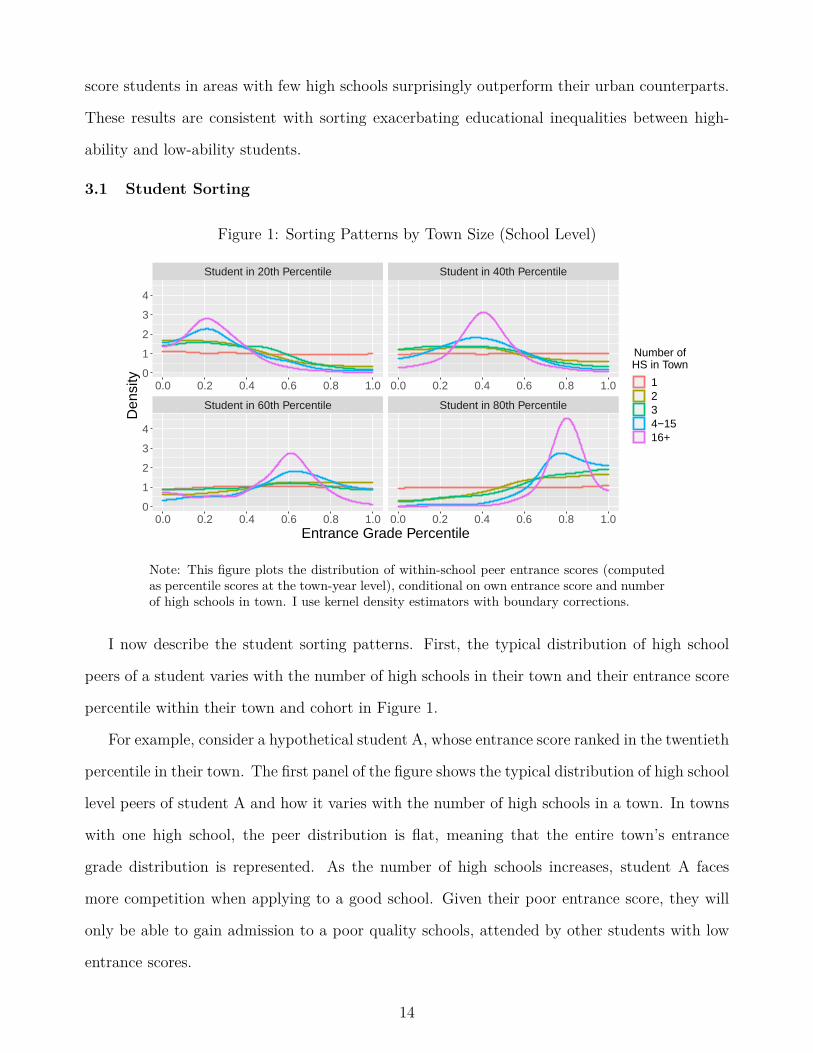
3.1 Student Sorting

Figure 1: Sorting Patterns by Town Size (School Level)

Student in 60th Percentile Student in 80th Percentile

Student in 20th Percentile Student in 40th Percentile

0.0 0.2 0.4 0.6 0.8 1.0 0.0 0.2 0.4 0.6 0.8 1.0

0.0 0.2 0.4 0.6 0.8 1.0 0.0 0.2 0.4 0.6 0.8 1.00

1

2

3

4

0

1

2

3

4

Entrance Grade Percentile

Den

sity

Number ofHS in Town

1234−1516+

Note: This figure plots the distribution of within-school peer entrance scores (computedas percentile scores at the town-year level), conditional on own entrance score and numberof high schools in town. I use kernel density estimators with boundary corrections.

I now describe the student sorting patterns. First, the typical distribution of high school

peers of a student varies with the number of high schools in their town and their entrance score

percentile within their town and cohort in Figure 1.

For example, consider a hypothetical student A, whose entrance score ranked in the twentieth

percentile in their town. The first panel of the figure shows the typical distribution of high school

level peers of student A and how it varies with the number of high schools in a town. In towns

with one high school, the peer distribution is flat, meaning that the entire town’s entrance

grade distribution is represented. As the number of high schools increases, student A faces

more competition when applying to a good school. Given their poor entrance score, they will

only be able to gain admission to a poor quality schools, attended by other students with low

entrance scores.

14

Figure 2: Student vs High School Peer Entrance Grades

−40

−30

−20

−10

0

10

20

30

40

50

1 2 3 4 5 6 7 8 9 10Student Own Entrance Grade Decile

Sch

ool A

vera

ge E

ntra

nce

Gra

de

Number ofHS in Town

One HS Town

Small Towns

Medium Towns

Large Towns

Note: This figure shows the relationship between student own high school entrance scoreand average peer entrance within the same high school, and how this relationship variesby town size and student entrance score. Specifically, it plots δd + δn + δd×n for differentcombinations of d and n in equation 1. Small Towns have 2-6 HS, Medium Towns have7-15 HS, Large Towns have 16+ HS.

At the other end of the spectrum, in the last panel of Figure 1, I plot the typical high school

peer distribution of student B, whose entrance score ranked in the eightieth percentile within

their town. In a one high school town, B’s typical peers will be no different than A’s, as all

students attend the same high school. However, in towns with more high schools, B’s high

entrance score will enable them to gain admission to a more selective school, where their peers

will also have high entrance grades.

Next, to get a more tangible sense of the extent to which students sort into high schools, I

regress student entrance scores on average entrance scores within their schools. I also interact

student ability with number of high schools to capture how peer entrance scores vary by student

entrance score, number of high schools in town of attendance and town population. Specifically,

I estimate the following model, which should capture differences in peer scores across student

15

ability and town characteristics:

µe−ihy =β0 + δd + δn + δd×n + δy + δp + δl + εi (1)

where µehy is the high school entrance score mean in high school h and year y and I use the

following fixed effects: entrance score decile of student i within their cohort, nationally (δd),

number of high schools in town l where student attends high school (δn), the interaction between

number of high school and student entrance decile (δd×n), year (δy), type of high school track or

program (δp) and town or location (δl). The results are presented in Table 9 of the Appendix

and illustrated in Figure 2.

Figure 3: Across- and Within-School Student Sorting

0.25

0.50

0.75

1 2 3 4 5 to 9 10 to 15 16 to 19 20 or MoreNumber of HS in Town

Ow

n vs

Pee

r E

ntra

nce

Gra

de S

core

Cor

rela

tion

Level

SchoolTrack

Note: This figure shows the distribution of the correlations between own admission scoresand peer scores (within tracks and within schools), across towns with different numbersof high schools.

Students in the highest decile in large towns attend schools with average entrance scores

that are 33 percentiles higher than their one high school town counterparts. At the other end

of the spectrum, students with bottom decile entrance scores in cities attend schools where the

average entrance grade is 27 percentiles lower than their rural counterparts. In large cities, the

average entrance score difference between the typical school attended by high-ability students

and those attended by low-ability students is 66 percentiles. In one high school towns, this

16

difference shrinks to a mere 6 percentiles.14

In terms of between-school and within-school sorting, the advantage of the Romanian high

school admission system is that students apply directly to tracks, so within-school sorting is

transparent. Figure 3 illustrates the correlation patterns between students and their peers’

entrance scores, at the high school and high school-track levels and how these vary across towns

with different numbers of high schools. In Appendix C, I show that student sorting occurs

principally at high school level, rather than at the track or classroom level. Even in towns with

few high schools, between-track sorting is limited and does not make up for students having

limited high school choices.

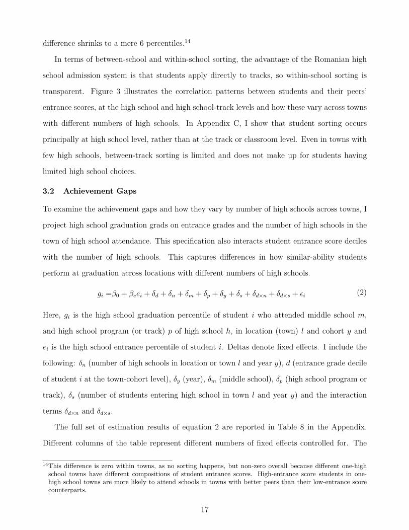
3.2 Achievement Gaps

To examine the achievement gaps and how they vary by number of high schools across towns, I

project high school graduation grads on entrance grades and the number of high schools in the

town of high school attendance. This specification also interacts student entrance score deciles

with the number of high schools. This captures differences in how similar-ability students

perform at graduation across locations with different numbers of high schools.

gi =β0 + βeei + δd + δn + δm + δp + δy + δs + δd×n + δd×s + εi (2)

Here, gi is the high school graduation percentile of student i who attended middle school m,

and high school program (or track) p of high school h, in location (town) l and cohort y and

ei is the high school entrance percentile of student i. Deltas denote fixed effects. I include the

following: δn (number of high schools in location or town l and year y), d (entrance grade decile

of student i at the town-cohort level), δy (year), δm (middle school), δp (high school program or

track), δs (number of students entering high school in town l and year y) and the interaction

terms δd×n and δd×s.

The full set of estimation results of equation 2 are reported in Table 8 in the Appendix.

Different columns of the table represent different numbers of fixed effects controlled for. The

14This difference is zero within towns, as no sorting happens, but non-zero overall because different one-highschool towns have different compositions of student entrance scores. High-entrance score students in one-high school towns are more likely to attend schools in towns with better peers than their low-entrance scorecounterparts.

17

baseline model has a full set of fixed effects, except town fixed effects (column (6)). Given that

the many interaction terms in this model, I graph out students’ predicted graduation scores

based on their entrance scores and the number of high schools in their town based on the

regression results (Figure 4).

Figure 4: Predicted Graduation Percentile by Town Size and Entrance Decile

0

10

20

30

40

50

60

70

1 2 3 4 5 6 7 8 9 10Entrance Grade Decile

Gra

duat

ion

Gra

de P

erce

ntile

Numberof High

Schools inTown

1234−1516+

Note: This figure plots the expected graduation percentile using the town size, entrancedecile (within town cohort) and their interaction, i.e. δd+δn+δd×n from equation 2. I alsouse a student’s expected entrance percentile conditional on their town size and entrancegrade decile (i.e. βeE[ei|dly(ei), nly]) so that the estimates are not driven by differences inentrance grade within deciles across towns with different numbers of high schools. I plotthe 95% confidence interval bounds.

The regression results show that, first, the graduation score gap between students in many-

high school towns and those of similar ability in few-high school towns is increasing in entrance

scores. For example, students whose entrance score is in the top decile in towns with more

than 15 high schools score, on average, 16 percentiles higher on the graduation exam than their

counterparts in towns with only one high school. Second, at the other end of the spectrum,

students who entered high school in the bottom decile in many-high school towns score 3 per-

centiles lower on the graduation exam than similar students in one high school towns. Third,

the graduation gap between high- and low-ability students within towns increases in the number

of high schools. While the graduation gap between students who scored in the highest decile

(nationally) on the entrance exam and those who scored in the bottom decile is 42 percentiles

18

in one high school towns, this figure is 63 percentiles in cities.

The reader should note that the graduation gaps described here vary with the number of

schools even though I include an interaction term between student ability and the number

of students in a town. This specification thus addresses the concern that these graduation

gaps occur because of different socioeconomic inequality levels, for example, between students

living in large towns and students living in smaller towns. There is a strong sense that even

conditional on town population or student population, the number of schools in a town is crucial

in explaining the graduation gap.

Moreover, the results indicate that the largest differences in graduation score gaps do not

occur between students in large, many-high school towns and very small, few-high school towns.

Instead, the largest differences in graduation gaps across ability occur between towns with one

high school and towns with two high schools. This is true even though the differences in these

towns’ populations and socioeconomic characteristics are plausibly much smaller than between,

say, towns with two high schools and large cities. These differences in graduation gaps are

mainly driven by differences in the number of high schools rather than by differences in town

size.

One of this paper’s main objectives is to explain why graduation score gaps follow the pat-

terns described above. I hypothesize that, given the competitive admission system in Romania,

different numbers of schools across locations mechanically give rise to starkly different student

sorting patterns. These sorting patterns are ultimately responsible for the observed graduation

gaps.

The intuition is that, in one high schools towns, sorting along ability is impossible.15 All the

students in these towns attend the same high school and their peers have entrance scores from

all across the entrance grade distribution. On the other hand, in towns with two high schools,

students can sort along ability. To the extent that some consensus exists about which school is

more desirable and given that high entrance score students receive priority, one would expect

to see a large degree of sorting along entrance grades. Looking at towns with higher number of15Except for migrating to a town with more high schools, which is costly and uncommon in the data. Moreover,in an alternate specification, I define education markets endogenously based on migration patterns in order toalleviate this issue. I also exclude students who migrate between these markets.

19

high schools, the potential for sorting is even greater. Still, the largest increase in the potential

for sorting is between towns with one high school and towns with two high schools.

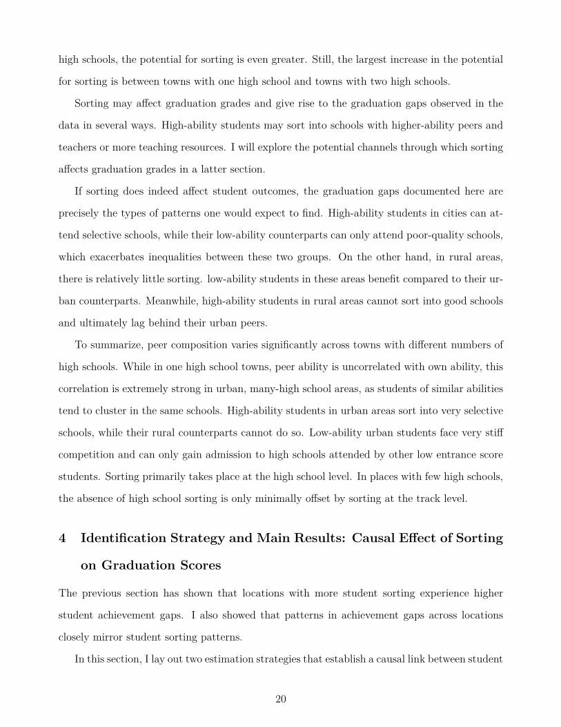
Sorting may affect graduation grades and give rise to the graduation gaps observed in the

data in several ways. High-ability students may sort into schools with higher-ability peers and

teachers or more teaching resources. I will explore the potential channels through which sorting

affects graduation grades in a latter section.

If sorting does indeed affect student outcomes, the graduation gaps documented here are

precisely the types of patterns one would expect to find. High-ability students in cities can at-

tend selective schools, while their low-ability counterparts can only attend poor-quality schools,

which exacerbates inequalities between these two groups. On the other hand, in rural areas,

there is relatively little sorting. low-ability students in these areas benefit compared to their ur-

ban counterparts. Meanwhile, high-ability students in rural areas cannot sort into good schools

and ultimately lag behind their urban peers.

To summarize, peer composition varies significantly across towns with different numbers of

high schools. While in one high school towns, peer ability is uncorrelated with own ability, this

correlation is extremely strong in urban, many-high school areas, as students of similar abilities

tend to cluster in the same schools. High-ability students in urban areas sort into very selective

schools, while their rural counterparts cannot do so. Low-ability urban students face very stiff

competition and can only gain admission to high schools attended by other low entrance score

students. Sorting primarily takes place at the high school level. In places with few high schools,

the absence of high school sorting is only minimally offset by sorting at the track level.

4 Identification Strategy and Main Results: Causal Effect of Sorting

on Graduation Scores

The previous section has shown that locations with more student sorting experience higher

student achievement gaps. I also showed that patterns in achievement gaps across locations

closely mirror student sorting patterns.

In this section, I lay out two estimation strategies that establish a causal link between student

20

sorting along ability and student performance. I first use variation in sorting patterns across

towns brought about by the different high school numbers across towns in an instrumental

variable framework. Secondly, I deploy triple difference framework to analyze the disruption in

preexisting sorting patterns caused by school openings in towns with few high schools.

4.1 Causal Effect of Sorting on Grades at Graduation

4.1.1 Using Variation in Number of Schools (IV)

The model I first exploit in order to asses the impact of sorting on graduation grades is a

variation of the Manski (1993) peer effects model:

gi = β0 + βeei + βµµe-ihy + δn + δd + δl + δm + δp + δy + δs + δs×d + εi (3)

Here, gi is the student percentile on the high school graduation exam, ei is the student percentile

on the high school entrance exam and µ−ihy is the mean entrance grade in high school h and year

y (excluding student i). I include fixed effects denoted with δ. These include the following fixed

effects: δn (number of high schools in town), δd (entrance grade decile at the town-cohort level),

δl (town), δm (middle school), δp (high school track or program), δy (year), δs (the number

of students entering high schools in town l and year y) and interaction δs×d. Typically, this

model is used when estimating peer effects when group formation is random. In this paper, the

interpretation will be different.

In this specification, the variable µ−ihy will be used a proxy for school quality and not a peer

effect estimate. I assume that students are rational and seek admittance to good schools when

given the choice. Good schools may be defined by higher-scoring students or teachers, better

management or better learning resources, but, for the moment, I do not yet take a stand on

what exactly school quality means. Simply, I assume that, on average, schools that are able to

attract higher entrance score students are of higher quality than those with low-entrance score

students.

A more immediate concern is that in the Romanian high school setup, µ−ihy is endogenous,

as it results from a student choice. Endogeneity could be modeled as an omitted variable that

21

is correlated with the peer entrance scores. I model the error term in equation 3, as:

εi = ζfi + χi (4)

where fi are unobservable characteristics of individual i that impact high school performance and

is correlated with µ−ihy. One example of this is the motivation to attend university. Conditional

on entrance score, this may drive a student to seek a higher quality school, while also impacting

their motivation to perform well in school. This would bias the estimates of βµ upward and

overstate the importance of school quality on the graduation exam grade. The instrument I use

to address this issue is an interaction between the number of schools in the student’s town and

their ranking within the town,16 so that the first stage of the estimation is:17

µehy = γ0 + γeei + ηn + ηd + ηd×n + ηm + ηl + ηp + ηy + ηs + ηs×d + ξi (5)

The intuition follows. This instrument exploits variation in the number of high schools across

locations of similar populations. In places with more high schools, there is more potential for

sorting across schools, and high-ability students will, on average, attend a better (or high-

entrance score) high school. In contrast, low-ability students will attend worse (low-entrance

score) schools in locations with more high schools, ceteris paribus, as seen in Figure 4.

For example, Figure 5 illustrates how, high-entrance grade students are able to sort into more

selective high schools, on average, than their counterparts in towns with similar populations,

but fewer high schools. At the other end of the spectrum, low-entrance grade students are

relegated to less selective high schools in tows with more high schools.

Secondly, this instrument satisfies the exclusion restriction. In other words, for students

with the same entrance scores and attending high school in towns with the same number of

high schools, their in-town ranking and size of their town is plausibly uncorrelated with their

motivation or other personal characteristics which may affect their scores at graduation. More

formally, ηd×n is conditionally independent of fi and χi.

Another identifying assumption is that the number of high schools across locations of sim-

16i.e. dly(ei)× nl, abbreviated as d× n for notational simplicity.17Where the η variables represent fixed effects, in order to avoid confusion with the δ fixed effects in the secondstage.

22

Figure 5: Instrumental Variable: An Illustration

Note: This figure illustrates the way in which the instrument shifts the type of schoolstudents attend. In locations with more high schools (town A), high-entrance score stu-dents attend, on average, a more selective school than their counterparts in a similar-sizedtowns with fewer high school (town B). Low-entrance score students in towns with morehigh schools (A) are relegated to less selective schools than in locations with fewer highschools (B).

ilar sizes affects students grades only through the type of schools that students attend. In

other words, I assume that the number of high schools across locations of similar populations

is not correlated with other non-observable town-level characteristics that affect high school

performance gaps between high- and low-ability students.

One observation that alleviates this type of concern is related to school closures. Romania

underwent massive depopulation since the fall of the communist regime in 1989, affecting towns

heterogenously. However, school closures are extremely rare. Thus, there is a sense that the

number of high schools in a given town is determined by decades-old decisions that are divorced

from that town’s current economic, social and demographic realities and is very unlikely to be

systematically correlated with student performance gaps.

Figure 6 shows that there is significant overlap in number of high schools across towns with

similar incoming high school student populations. This variation is precisely the one captured

by the instrumental variable. Notice that this variation implies that school sizes across these

locations differ. However, classroom sizes are fixed at 28 students, typically and, since most

schools are oversubscribed, there variation in classroom size is not a major concern.

Lastly, for now, I assume that the effect of attending a better school on student performance

23

Figure 6: Number of Students vs Number of High Schools Across Towns

1

2

3

4

5

6

7

8

9

10−19

20−29

30−39

40+

1 10 100 1000 10000

Yearly Students Admitted to High Schools in Town

Hig

h S

choo

ls in

Tow

n

Note: This figure plots the distribution of the number of students admitted to high schoolsacross towns with different numbers of high schools. Notice that, while the number ofadmitted students is increasing in the number of high schools, there is significant overlapin the number of students across towns with different numbers of high schools.

is homogeneous for all students. This assumption will be relaxed later, when I study the channels

through which sorting affects student scores.

Several identification challenges, including sample selection and student migration issues,

are addressed later in the section. I conduct appropriate robustness checks in order to alleviate

concerns regarding them.

First Stage I estimate equation 3, using the interaction between student entrance score decile

(at the town-cohort level) and the number of high schools in the student’s town as an instrument

for the ability of his or her peers at the school (µ−ihy) and at the school-track levels (µ−ihpy).

As explained previously, the peer means and their corresponding estimates should not be inter-

preted as peer effects. Rather, they are proxies for school (or track) quality and may capture

superior teaching and school facilities, as well as peer effects.

Figure 7 and Table 10 (Table 11) in the Appendix present the first stage estimates at the

school (track) levels. The differences in sorting on entrance grades across towns with different

24

numbers of high schools are substantial. On average, lowest entrance grade decile students’

peers in one high school towns score 29 (15) percentiles higher than their counterparts in many-

high school towns. At the other end of the spectrum, highest entrance grade decile students’

peers in one high school towns score 28 (19) percentiles lower at high school entrance than their

counterparts in towns with at least 15 high schools.

F-statistics for weak instrument tests are computed for the first stages. All F-statistics are

extremely large and rule out weak instruments beyond any doubt. The F-statistics for school

(track) first stages are all larger than 297 (378). These far exceed the threshold derived by

Stock and Yogo (2002) for a maximum bias of 0.05.18 Moreover, these also exceed the more

conservative threshold of 104.7 recently developed by Lee et al. (2020).19

The first stage results suggest that sorting intensity within schools and tracks increases

rapidly in the number of high schools in a town, even when controlling for student population.

Intuitively, the instrumental variable picks up variation in the average peer entrance score of

students who have similar abilities and live in towns with similar student populations, but with

different numbers of high schools. This difference in sorting patterns is especially stark between

towns with one high school and towns with two high schools. For example, a high entrance

score student in a two high school town will typically attend the high school in their town with

a higher average entrance score. In contrast, an identical student in a similar-size town that

only has one high school will not be able to select into a high entrance grade high school.20

Thus, the average entrance score of this student’s peers will be significantly lower than that of

two-high school town counterpart.

To summarize, conditional on town population, I find that the ability of peers is increasing

both in own ability and in the number of high schools in the town for students who are above-

average. The competitive admission system works in their advantage and they are able to

sort into selective schools. For below-average student, average peer entrance score is increasing

18This stands at approximaetly 21.4 for 40 instruments and one endogenous variable.19Intuitively, Lee et al. (2020) find that unless the first stage F-statistic is at least 104.7, the true confidenceintervals of the second stage estimate of the β on the endogenous variable should be constructed using t-valueslarger than 1.96. In my setup, this is can be dismissed out of hand, since the F-statistics all far exceed thisthreshold.

20That is, without migrating to a different town. Migration is addressed later in this section.

25

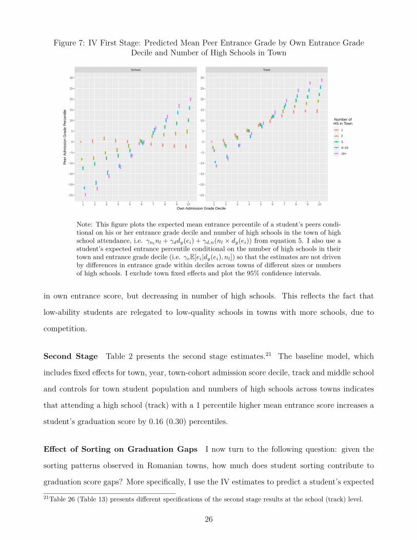
Figure 7: IV First Stage: Predicted Mean Peer Entrance Grade by Own Entrance GradeDecile and Number of High Schools in Town

School Track

1 2 3 4 5 6 7 8 9 10 1 2 3 4 5 6 7 8 9 10

−25

−20

−15

−10

−5

0

5

10

15

20

25

30

−25

−20

−15

−10

−5

0

5

10

15

20

25

30

Own Admission Grade Decile

Pee

r A

dmis

sion

Gra

de P

erce

ntile

Number ofHS in Town

1

2

3

4−15

16+

Note: This figure plots the expected mean entrance percentile of a student’s peers condi-tional on his or her entrance grade decile and number of high schools in the town of highschool attendance, i.e. γnl

nl + γddy(ei) + γd,n(nl × dy(ei)) from equation 5. I also use astudent’s expected entrance percentile conditional on the number of high schools in theirtown and entrance grade decile (i.e. γeE[ei|dy(ei), nl]) so that the estimates are not drivenby differences in entrance grade within deciles across towns of different sizes or numbersof high schools. I exclude town fixed effects and plot the 95% confidence intervals.

in own entrance score, but decreasing in number of high schools. This reflects the fact that

low-ability students are relegated to low-quality schools in towns with more schools, due to

competition.

Second Stage Table 2 presents the second stage estimates.21 The baseline model, which

includes fixed effects for town, year, town-cohort admission score decile, track and middle school

and controls for town student population and numbers of high schools across towns indicates

that attending a high school (track) with a 1 percentile higher mean entrance score increases a

student’s graduation score by 0.16 (0.30) percentiles.

Effect of Sorting on Graduation Gaps I now turn to the following question: given the

sorting patterns observed in Romanian towns, how much does student sorting contribute to

graduation score gaps? More specifically, I use the IV estimates to predict a student’s expected

21Table 26 (Table 13) presents different specifications of the second stage results at the school (track) level.

26

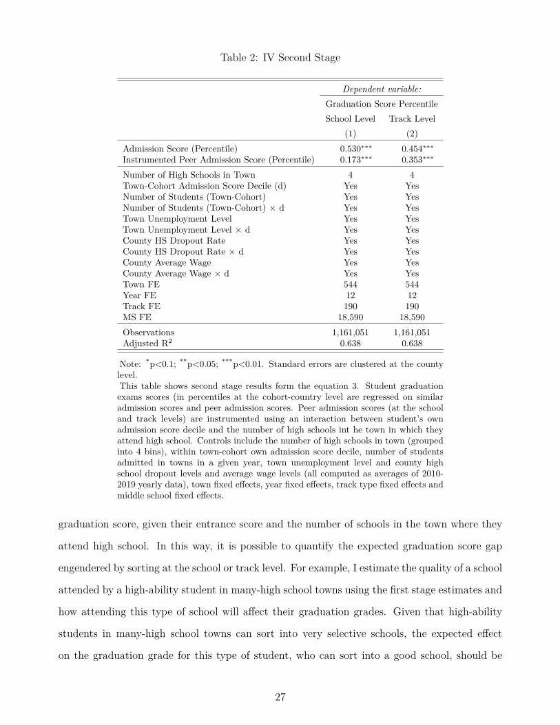
Table 2: IV Second Stage

Dependent variable:Graduation Score PercentileSchool Level Track Level

(1) (2)Admission Score (Percentile) 0.530∗∗∗ 0.454∗∗∗Instrumented Peer Admission Score (Percentile) 0.173∗∗∗ 0.353∗∗∗

Number of High Schools in Town 4 4Town-Cohort Admission Score Decile (d) Yes YesNumber of Students (Town-Cohort) Yes YesNumber of Students (Town-Cohort) × d Yes YesTown Unemployment Level Yes YesTown Unemployment Level × d Yes YesCounty HS Dropout Rate Yes YesCounty HS Dropout Rate × d Yes YesCounty Average Wage Yes YesCounty Average Wage × d Yes YesTown FE 544 544Year FE 12 12Track FE 190 190MS FE 18,590 18,590Observations 1,161,051 1,161,051Adjusted R2 0.638 0.638

Note: *p<0.1; **p<0.05; ***p<0.01. Standard errors are clustered at the countylevel.This table shows second stage results form the equation 3. Student graduationexams scores (in percentiles at the cohort-country level are regressed on similaradmission scores and peer admission scores. Peer admission scores (at the schooland track levels) are instrumented using an interaction between student’s ownadmission score decile and the number of high schools int he town in which theyattend high school. Controls include the number of high schools in town (groupedinto 4 bins), within town-cohort own admission score decile, number of studentsadmitted in towns in a given year, town unemployment level and county highschool dropout levels and average wage levels (all computed as averages of 2010-2019 yearly data), town fixed effects, year fixed effects, track type fixed effects andmiddle school fixed effects.

graduation score, given their entrance score and the number of schools in the town where they

attend high school. In this way, it is possible to quantify the expected graduation score gap

engendered by sorting at the school or track level. For example, I estimate the quality of a school

attended by a high-ability student in many-high school towns using the first stage estimates and

how attending this type of school will affect their graduation grades. Given that high-ability

students in many-high school towns can sort into very selective schools, the expected effect

on the graduation grade for this type of student, who can sort into a good school, should be

27

Figure 8: Predicted Mean Causal Effect of Sorting

School Track

1 2 3 4 5 6 7 8 9 10 1 2 3 4 5 6 7 8 9 10−6

−4

−2

0

2

4

6

8

10

12

−6

−4

−2

0

2

4

6

8

10

12

Admission Grade Decile

Gra

duat

ion

Gra

de P

erce

ntile

Number ofHS in Town

1

2

3

4−15

16+

Note: This figure plots the expected mean causal effect of sorting on graduation grade, byentrance grade decile and number of high schools in the town of high school attendance.This is computed as βµE[µ̂ehy|dly(ei), nl]]. I also plot the 95% confidence intervals.

positive. This contrasts with students of similar ability in few-high school towns, who will lack

the option of attending selective schools.

Specifically, I first use the first stage estimates to predict, based on student entrance score and

town they attend high school in, the school quality they attend.22 Then, given this estimate

of school quality, I use the second stage estimates to predict the estimated effect of sorting

on their grade at graduation.23 Note that, alternatively, I could have used the second stage

estimates directly with the realized school quality (µ−ihy) rather than using estimated school

quality (µ̂−ihy). However, given that school quality is endogenous, this would lead to a biased

estimate.24 I plot this estimate and corresponding confidence intervals for students in different

entrance deciles and attending high school in towns with different numbers of high schools.

I find that students in the sixth decile or above benefit from attending a high school (high

school track) in many-high school towns and this benefit increases in both in the number of high

22I compute µ̂−ihy = γnlnly + γddly(ei) + γd,n(nly × dly(ei)) + γeE[ei|dly, nly] from equation 5.

23More specifically, I compute βµµ̂−ihy24For example, if, conditional on entrance scores, more motivated students perform better in high school and alsotend to enroll into better schools, using this approach would lead to results that are upward biased. Indeed,this approach would capture the effect of attending a better school via sorting, but also the effect of havinghigher motivation.

28

schools and student entrance score. On the other hand, students in the third decile or lower in

their town are better off attending high school in towns with fewer high schools. It turns out

that in cities, students in the top entrance grade decile receive a 7 (12) percentile boost on their

graduation grade from sorting, on average.25 This is in contrast to the 3 (7) percentile increase

seen by their high-ability counterparts in one high school towns, who are penalized by not being

able to choose more selective high schools. At the other end of the spectrum, students in the

lowest entrance grade decile who attend high school in large cities receive a 4 (4) graduation

grade percentile penalty from sorting when compared to their counterparts in one high school

towns.

Moreover, in large cities, the high levels of sorting at the school (track) levels lead to a 12

(17) percentile widening of the performance gap between top entrance score decile students and

their counterparts in the lowest decile. In towns with only one high school, this figure shrinks

to 3 (7) percentiles.

Significantly, these result is not driven by students with similar admission scores performing

differently in towns of different populations. By controlling for student population in towns and

interacting it with individual student admission scores, the model allows students with similar

admission scores living in towns with different populations to have different graduation scores.

The identifying variation is thus variation in graduation grades of students of similar abilities

across towns with similar populations, but different numbers of high schools.

To summarize, increasing levels of sorting are accountable for a widening in graduation

score gaps between high- and low-ability students within towns. Second, sorting widens the

performance gap between urban high-ability students (who can attend selective schools) and

rural high-ability students (who cannot). The gap between low-ability urban students (who

attend the worst urban schools) and low-ability rural students (who benefit from low sorting in

rural areas) shrinks via sorting.

25Compared to the baseline case of students in the lowest decile in one high school towns.

29

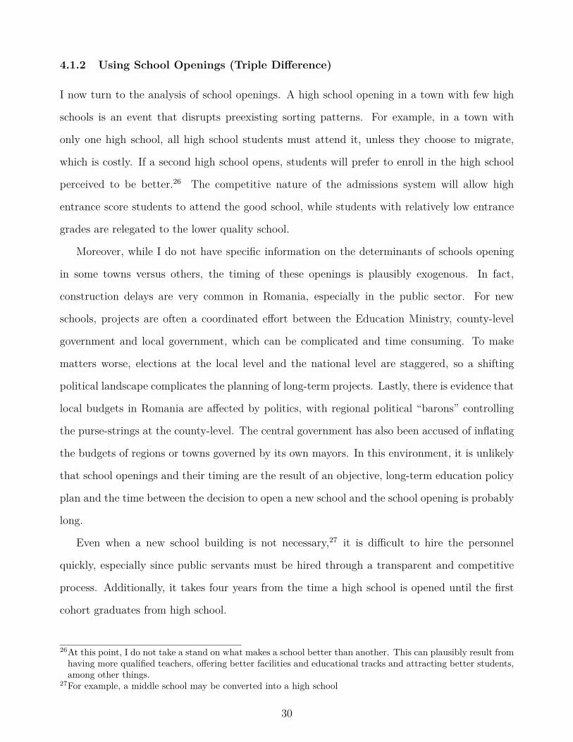
4.1.2 Using School Openings (Triple Difference)

I now turn to the analysis of school openings. A high school opening in a town with few high

schools is an event that disrupts preexisting sorting patterns. For example, in a town with

only one high school, all high school students must attend it, unless they choose to migrate,

which is costly. If a second high school opens, students will prefer to enroll in the high school

perceived to be better.26 The competitive nature of the admissions system will allow high

entrance score students to attend the good school, while students with relatively low entrance

grades are relegated to the lower quality school.

Moreover, while I do not have specific information on the determinants of schools opening

in some towns versus others, the timing of these openings is plausibly exogenous. In fact,

construction delays are very common in Romania, especially in the public sector. For new

schools, projects are often a coordinated effort between the Education Ministry, county-level

government and local government, which can be complicated and time consuming. To make

matters worse, elections at the local level and the national level are staggered, so a shifting

political landscape complicates the planning of long-term projects. Lastly, there is evidence that

local budgets in Romania are affected by politics, with regional political “barons” controlling

the purse-strings at the county-level. The central government has also been accused of inflating

the budgets of regions or towns governed by its own mayors. In this environment, it is unlikely

that school openings and their timing are the result of an objective, long-term education policy

plan and the time between the decision to open a new school and the school opening is probably

long.

Even when a new school building is not necessary,27 it is difficult to hire the personnel

quickly, especially since public servants must be hired through a transparent and competitive

process. Additionally, it takes four years from the time a high school is opened until the first

cohort graduates from high school.

26At this point, I do not take a stand on what makes a school better than another. This can plausibly result fromhaving more qualified teachers, offering better facilities and educational tracks and attracting better students,among other things.

27For example, a middle school may be converted into a high school

30

I use a triple difference (DDD) approach to compare the differences in graduation grades

of high entrance score students versus low entrance score students, in towns of where a new

school was opened versus towns with no new schools, before and after the school opening. Since

schools open in different years for different towns, it is impossible to define a before and after

opening period. Following Wooldridge (2002), I adopt the standard approach of staggered DDD,

including time dummies, town dummies and all pairwise interactions with the quartiles. The

equation I estimate is:

gi =β0 + βeei + βTT + δq + δl + δy + δqy + δlq + δs + ηs×q + δTq + εi (6)

Here, gi is the student percentile on the high school graduation exam, ei is the student entrance

grade percentile and fixed effects are denoted by δ. These include: the entrance grade quartile

within town-year of student i (δq), town (δl), year (δy), quartile-year (δqy), town-quartile (δlq),

number of students in a town in a cohort (δs), number of students in the town-cohort interacted

with a student’s entrance grade quartile (δq×s) and treatment-year (δTy) . I also include Tly

(the treatment variable, abbreviated T ), a dummy variable indicating whether or not town l

was subject to a school opening before or during year y. It is non-zero only for treated towns

after a new school opens. Note that the inclusion of the interaction term δq×s means that the

model is flexible, allowing students with similar entrance grades to perform differently in towns

with different populations.

An alternate specification, using the relative number of seats in the opening high school

relative to the town’s preexisting seats as a treatment variable, instead of a simple treatment

dummy, is estimated and results are presented in the Appendix (Table 14).28

For this estimation, I restrict my attention to towns with either one or two high schools in

the pre-period. Indeed, the opening of one high school in many-high school towns is unlikely

to disrupt the preexisting sorting patterns in that town sufficiently. Moreover, I exclude the

28In this alternative specification, the treatment variable T and it is computed as the number of seats in anewly-opened school relative to the number of seats in the old schools of that town. For example, if a townl has 1,000 seats and a new school with 100 seats opens in year y, T will take a value of 0.1 for town l andany year including and after y. It will take a value of zero for any town before a new school is built and forany town in which there are no school openings. The DDD coefficient of interest is δTq. It captures how thethe difference in graduation scores between students in different entrance score quartiles evolves after a schoolopening in a town versus before the opening compared to towns where there was no school opening.

31

Figure 9: DDD: Sorting Patterns Before and After School Opening (Treatment Group), byEntrance Score

Student in 90th Percentile Student in 99th Percentile

Student in 50th Percentile Student in 75th Percentile

Student in 10th Percentile Student in 25th Percentile

0.00 0.25 0.50 0.75 1.00 0.00 0.25 0.50 0.75 1.00

0

1

2

3

4

0

1

2

3

4

0

1

2

3

4

Entrance Grade (Percentile)

Den

sity Timing

After Opening

Before Opening

Note: This figure plots the distribution of student peers (within the same school) in thetreatment group, conditional on own entrance score, before and after high school opening.

openings of schools that are not suitable substitutes for preexisting schools (e.g. religious high

schools29 and high schools where teaching is conducted in a foreign language30) and schools that

already existed in a different form (e.g. vocational or other type of schools and were changed

into high schools). Table 15 of Appendix A provides more information on the school openings

retained for this analysis.

The triple difference results follow. As noted previously, this approach exploits disturbances

in sorting patterns caused by school openings in few-high school towns. Figures 9 and 13 in

the Appendix show the changes in sorting patterns before and after high school openings in

the treatment and control groups, respectively. The control group shows very little change over

time in the distribution of peers conditional on entrance score. In contrast, the changes in the

treatment group sorting patterns are quite stark. In particular, the high school opening seem-29These can have different denominations, the main ones being Greek Orthodox, Roman Catholic and GreekCatholic. In addition, some of these are exclusive to boys or girls.

30Typically, Hungarian or German, the two largest minority languages in Romania.

32

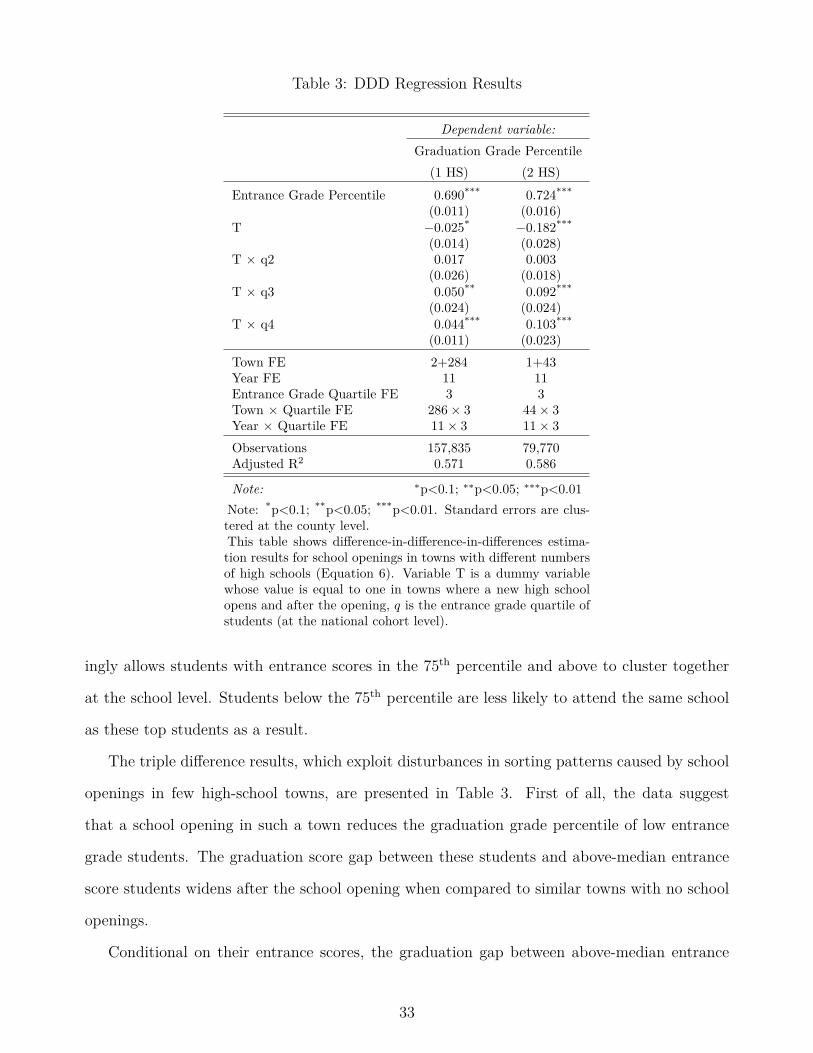
Table 3: DDD Regression Results

Dependent variable:Graduation Grade Percentile

(1 HS) (2 HS)Entrance Grade Percentile 0.690*** 0.724***

(0.011) (0.016)T −0.025* −0.182***

(0.014) (0.028)T × q2 0.017 0.003

(0.026) (0.018)T × q3 0.050** 0.092***

(0.024) (0.024)T × q4 0.044*** 0.103***

(0.011) (0.023)Town FE 2+284 1+43Year FE 11 11Entrance Grade Quartile FE 3 3Town × Quartile FE 286× 3 44× 3Year × Quartile FE 11× 3 11× 3Observations 157,835 79,770Adjusted R2 0.571 0.586

Note: ∗p<0.1; ∗∗p<0.05; ∗∗∗p<0.01Note: *p<0.1; **p<0.05; ***p<0.01. Standard errors are clus-tered at the county level.This table shows difference-in-difference-in-differences estima-tion results for school openings in towns with different numbersof high schools (Equation 6). Variable T is a dummy variablewhose value is equal to one in towns where a new high schoolopens and after the opening, q is the entrance grade quartile ofstudents (at the national cohort level).

ingly allows students with entrance scores in the 75th percentile and above to cluster together

at the school level. Students below the 75th percentile are less likely to attend the same school

as these top students as a result.

The triple difference results, which exploit disturbances in sorting patterns caused by school

openings in few high-school towns, are presented in Table 3. First of all, the data suggest

that a school opening in such a town reduces the graduation grade percentile of low entrance

grade students. The graduation score gap between these students and above-median entrance

score students widens after the school opening when compared to similar towns with no school

openings.

Conditional on their entrance scores, the graduation gap between above-median entrance

33

score students and their low entrance score counterparts widens by 4 to 10 percentiles in towns

where a new high school opened compared to towns with no new openings.31 Perhaps even more

worryingly, there is evidence suggesting that conditional on entrance scores, school openings

decrease graduation scores, on average.

These findings suggest that school construction benefits are not equally distributed among

students of different abilities. While Duflo (2001) uses Indonesian data to suggest that school

construction has strong and persistent effects on average educational outcomes and wages, the

Romanian data suggest that, at least in a context in which there is school choice, high-ability

students disproportionately absorb these gains. Meanwhile, low-ability students may actually be

negatively impacted by school construction, as they become more segregated from their high-

ability counterparts. Overall, the results indicate a possible decrease in average graduation

scores in towns where new high schools open.

To summarize, both using differences in numbers of high schools across locations and high

school openings confirm the causal link between increases in sorting and increases in achievement

gaps between high- and low-entrance grade students. In the following sections, I explore the

possible channels through which sorting plausibly affects student achievement.

4.1.3 Identification Concerns and Robustness Checks

Town Size A potential issue with identification is that the number of high schools corre-

lates with other underlying, unobserved town-level characteristics that are the main drivers of

increasing grade inequality.

For example, in towns with more high schools, socioeconomic inequality between high en-

trance score and low entrance score students may be higher. This inequality could then explain

the increasing graduation gaps. Low entrance score students in large, many-high school towns

may be poorer, face more social exclusion, on average, than their counterparts in small, few-

high school towns, which may later have a bearing on their scores at graduation. Adding middle31In the alternate specification, I estimate that the opening of a new school which accounts for 10% extra seatsin that town will cause a 2 to 4 percentile widening of the gap between lowest-quartile students and theirabove-median counterparts post-opening in one and two high school towns, respectively. This is consistentwith entrance grade sorting heterogeneously affecting student results post-opening. As before, higher levels ofsorting are detrimental to low entrance score students and benefit high entrance score students.

34

school fixed effects partially addresses this concern. Middle schools in Romania are more numer-

ous than high schools and typically serve a relatively narrow geographic area, especially in cities.

Thus, middle school fixed effects can control for neighborhood-specific average characteristics.

Moreover, if student selection into towns driven by unobservable characteristics and socioe-

conomic differences unaddressed by middle school fixed effects are real concerns, controlling

for the student populations in towns and interacting it with student abilities mitigates these

issues. These interaction terms add extra flexibility to the model. They capture differences in

the performance of students with similar entrance scores across towns of different populations.

Once these controls are introduced, the instrument captures only differences in sorting patterns

mechanically resulting from differences in high school numbers across locations, conditional on

town populations.

Migration Another issue is migration. Given the institutional setup in Romania, where

there are no school districts, there are no barriers preventing students from migrating to attend

a specific high school. The concern is that more motivated or academically inclined students

sort into larger, many-high school towns to attend better schools, which would bias results.

I propose two solutions to this problem. First of all, geographic migration is limited. Indeed,

roughly 70% of all high school students attend a high school at most 10 km away from their

middle school, while over 90% of them attend a high school at most 30 km away from the middle

school they attended. In this sense, even if there is migration, the data suggest it is limited in

scope and that the hometown of a student plays a big role in the type of school they attend.

Second, I estimate an alternate specification to the IV estimation. Instead of using towns

as separate educational markets, I define these markets endogenously. For example, if a non-

negligible number of students32 graduating from a middle school attend high schools in town A,

I consider this middle school to be part of the same educational market, even if it is not loacted

in the same town. Moreover, if sufficiently many students from other middle schools enroll in

high schools in both town A and B, then both towns A and B will be considered part of the

32In practice, I use different specifications to decide this threshold. However, these do not affect the estimatedIV results significantly.

35

same market. I then reestimate the IV specification, replacing towns with these endogenous

markets. I also estimate this new specification after excluding all students who migrate (i.e.

who attend high school in a different market than their middle school; there are approximately

7% of these in my data). The second stage results are presented in Tables ?? to ?? of the

Appendix. The results are very robust to these different specifications. Indeed, attending a

high school (high school track) with a one percentile higher average entrance score causes an

average score increase of 0.15 (0.30) percentiles when using the number of high schools across

market rather than across towns as instruments. This estimate is 0.13 (0.27) percentiles when

excluding across-market migration.

Sample Selection Lastly, there is a possible sample selection issue: I can only observe the

graduation grades of students who write the graduation exam and not of those who drop out

of high school. In order to address this, I use a Heckman two-stage correction for models with

endogenous variables. The idea behind this approach is to use an instrument that, conditional

on other covariates, can predict a student’s probability of dropping out without directly affecting

their grades. I use the proportion of high school dropouts in a student’s middle school peers.

The intuition is that conditional on entrance grade, this instrument does not affect high school

performance, but observing middle school peers dropping out may dissuade a student (or their

parents) from exerting extra effort to keep the child in high school. Although there is some

evidence of sample selection, the results adjusted for sample selection are qualitatively similar

to the unadjusted ones. For more details, consult Appendix D.

5 Decomposing Sorting Effects

In this section, I analyze three possible channels through which student sorting plausibly impacts

grades. First, student sorting may directly impact scores via peer or social effects. Second, high

entrance score students may sort into schools with higher ability teachers, which would likely

improve their graduation scores. Third, high entrance score students may sort into schools with

better classroom learning facilities or better infrastructure.

36

5.1 Sorting Patterns

5.1.1 Teacher Sorting

I now turn to teacher sorting. Teacher sorting patterns display two main trends. These are are

summarized in Table 4. The first trend is that teachers sort on test scores both across towns

and within towns. Second, high-scoring teachers disproportionately work in schools attended

by high-admission score students.

To be more specific, higher test score teachers are more likely to work in larger towns, as

shown in the first row of the table. While teachers in locations with one high school on average

score in the 47th percentile on their placement exam, this figure is the 54th percentile in locations

with 16 or more high schools. Teacher sorting by test scores across high schools is strong. Across

towns with similar numbers of high schools (row 2), the palcement scores of coworkers teaching

the same subject display a correlation of around 0.25, regardless of town size. Within towns

(row 3), sorting is far more pronounced in localities with many high schools. These two findings

together suggest that in smaller towns, there is significant across-town sorting of teachers on

placement scores, but but less within-town sorting. For many-high school locations, teachers

sort on placement scores across high schools, but not so much across towns.

Moreover, teacher sorting mirrors student sorting, with higher-scoring teachers dispropor-

tionately teaching high entrance-score students. Rows 4 suggests that high-scoring teachers

are hired by schools attended by high-scoring students and this effect is more pronounced in

locations with many high schools, where access to good teachers is particularly difficult for

low-scoring students.

In summary, there is evidence of teacher sorting. High-scoring teachers tend to sort into the

same schools and these schools are disproportionately urban, more selective schools. The two

findings are important. To the extent that teacher placement scores correlate with teacher value-

added, this raises concerns about inequalities due to school choice. Indeed, the implication is

that high-scoring students will be able to sort into schools with high-scoring teachers and receive

a better education, while low-scoring students will farther be penalized by being segregated into

37

schools not only with lower-achieving peers, but with less competent teachers.

Table 4: Teacher Sorting

Number of High Schools in Town 1 2 3 4-15 16+

Average Teacher Score (Percentile) 47 47 49 49 54

Teacher-Coworker Score Correlation 0.25 0.23 0.32 0.27 0.29

Average within-Town Teacher-Coworker Score Correlation −0.11 0.13 0.23 0.21 0.30

Teacher-Student Score Correlation 0.04 0.11 0.07 0.12 0.14

a

5.1.2 School Spending

Next, I investigate whether high entrance score students attend high schools that spend rel-

atively more money per student. This may either be due to students preferring high schools

which spend more per capita or, alternatively, schools who attract high entrance score students

may be able to harness more financial resources for their students subsequently.

Either way, if student sorting is correlated to school expenditures, one should observe high

entrance grade students disproportionately attending high budget schools. In order to study

this, I estimate several versions of the following model, for student i attending high school h:

exph =β0 + δd + δn + δl + δy + δd×n + εi,h (7)

Here, exph is the average annual per-student expenditure of high school h. Fixed effects are

denoted by δ. They include: δd (entrance grade decile), δn (number of high schools in town), δl

(town), δy (year) and δd×n (town size-entrance score decile).

The results are presented in Figure 10 and Table 18 in the Appendix. The results suggest

several interesting patterns in the school expenditures. First, low-entrance score students receive

more money per capita than their high-entrance score counterparts. Indeed, top decile students

receive €25 per capita per year less than the bottom decile students.33 This suggests that the

government is making efforts to target spending towards disadvantaged students.

33The average amount is €30 per student per year and the standard deviation is roughly €60.

38

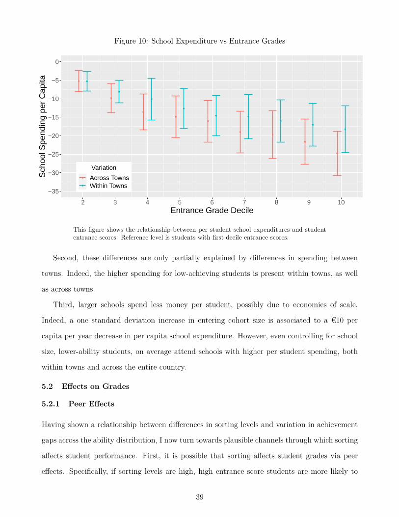
Figure 10: School Expenditure vs Entrance Grades

−35

−30

−25

−20

−15

−10

−5

0

2 3 4 5 6 7 8 9 10Entrance Grade Decile

Sch

ool S

pend

ing

per

Cap

ita

Variation

Across TownsWithin Towns

This figure shows the relationship between per student school expenditures and studententrance scores. Reference level is students with first decile entrance scores.

Second, these differences are only partially explained by differences in spending between

towns. Indeed, the higher spending for low-achieving students is present within towns, as well

as across towns.

Third, larger schools spend less money per student, possibly due to economies of scale.

Indeed, a one standard deviation increase in entering cohort size is associated to a €10 per

capita per year decrease in per capita school expenditure. However, even controlling for school

size, lower-ability students, on average attend schools with higher per student spending, both

within towns and across the entire country.

5.2 Effects on Grades

5.2.1 Peer Effects

Having shown a relationship between differences in sorting levels and variation in achievement

gaps across the ability distribution, I now turn towards plausible channels through which sorting

affects student performance. First, it is possible that sorting affects student grades via peer

effects. Specifically, if sorting levels are high, high entrance score students are more likely to

39

have high-ability schoolmates or classmates. Low entrance score students are more likely to

have schoolmates or classmates that are of low-ability. To the extent that students generate

learning spillovers that affect their peers’, high levels of sorting can create virtuous feedback

loops for high-ability students and negative feedback loops for low-ability students.

To estimate the peer effects, I use the year to year variation in the entrance grades of different

cohorts within the same school. The idea is that, if school quality34 is relatively stable over

time, then the differences in average entrance score within a school from one year to another are

quasi-random. Indeed, given the relatively small number of students admitted to a given high

school in a given year, one would expect small, random deviations in entering cohort ability

from year to year. This assumption can break down if unobserved school characteristics change

over time and the student applicant pool also changes in response to this. However, anecdotally

speaking, the rankings of high schools in Romania are quite persistent and the admission system

enforces this persistence: a good school attracts top students and top teachers, which in turn

creates a virtuous cycle, attracting more high-scoring students and teachers. In order to capture

peer effects, the estimated equation is:

gi =β0 + βeei + βµµe−ihy + δl + δh + δm + δp + δy + δs + δd+

δn + δn×d + δh×p + δs×d + εi

(8)

Here, gi is student i’s high school graduation percentile, ei is their high school entrance per-

centile, µe−ihy is the peer mean entrance percentile in high school h and cohort y, excluding

student i. Fixed effects are denoted by δ. I include the following fixed effects: town (δl), high

school (δh), middle school (δm), high school track or program type (δp), year (δy), number of

high school students admitted in town l and year y (δs), entrance decile within town-year (δd),

number of high schools in town (δn) and interactions δn×d, δh×p and δs×d.

While µe−ihy is endogenous because it directly results from a student decision to enroll in

high school h, conditioning on high school and track fixed effects (δh×p) means that βµ will be

identified by the yearly variation in the average entrance grade of students within high school

tracks, which I assume to be quasi-random. If the quasi-randomness assumption is true, then

34In terms of facilities, teachers or any other factor that impacts student achievement except for peer effects.

40

conditional on high school, βµ will be the coefficient of interest and will capture peer effects on

the student graduation grades.

The estimation results for the peer effects regressions are presented in Table 5, where a

student’s peers are defined as students entering the same track, within the same high school,

in the same year. The most relevant model is the full-fixed effects models and are presented

in columns (5) of table 5. In this specification, I am comparing students enrolled in the same

track within the same high schools, but who happen to have peers of different abilities. As a

robustness check, similar models are estimated at the high school, rather than high school-track

level.35 Once all fixed effects are included, the results suggest the absence of a meaningful

relationship between variations in peer ability and student graduation scores.

Lastly, in order to allow for possible heterogeneity in the peer effects, I estimate and alterna-

tive specification in which I interact the student’s relative ranking within their school’s entering

cohort with the peer average entrance score:36

gi =β0 + βeei + βµµe−ihy + δl + βµ,d(µe−ihpy × dhpy(ei)) + δh + δm + δp + δy + δs + δd+

δn + δn×d + δh×p + δs×d + εi

(9)

The estimated results are shown in Table 20 in the Appendix and illustrated in Figure 11.

The peer effects increase with a student’s rank within their entrance grade track (or school).

Only high entrance score students benefit from increases in cohort ability, while lower entrance

score students are negatively affected by having stronger peers. This is consistent with survey

results by Pop-Eleches and Urquiola (2013), who show that students near the entrance score

thresholds in Romania are more likely to face bullying, social exclusion and low confidence of

their ability than students with similar grades who attend less selective schools. This type of

heterogeneity in peer effects is consistent with the single crossing peer effects models, as per

Sacerdote (2011).

35Results are presented in Table 19 of the Appendix.36Where gi is student i’s high school graduation percentile, ei is their high school entrance percentile, µe−ihyis the peer mean entrance percentile in high school h and cohort y, excluding student i and the followingfixed effects are included: town (δl), high school (δh), middle school (δm), high school track or program type(δp), year (δy), number of high school students admitted in town l and year y (δsly

, abbreviated δs), entrancedecile within town-year (δdly

, abbreviated δd), number of high schools in town (δnly, abbreviated δn) andinteractions δn×d, δh×p and δs×d. Lastly, I include an interaction term µe−ihpy × dhpy(ei) (interaction betweenstudent ability and peer ability at high school entrance) that will capture heterogeneities in peer effects.

41

Table5:

Peer

Effects

Regression(T

rack

Level)

Dep

ende

ntva

riab

le:

Gradu

ationEx

amPe

rcentile

(1)

(2)

(3)

(4)

(5)

(NoHS,HS-Tr

ackFE

)En

tran

ceGrade

Percentile

0.53

2∗∗∗

0.53

6∗∗∗

0.51

5∗∗∗

0.51

5∗∗∗

0.53

1∗∗∗

0.53

1∗∗∗

(0.0

32)

(0.0

32)

(0.0

21)

(0.0

21)

(0.0

19)

(0.0

19)

MeanEn

tran

cePe

rcentile(H

S-Tr

ack-Coh

ort)

−0.

063∗∗

∗−

0.06

6∗∗∗

−0.

009

−0.

009

−0.

017

−0.

017

(0.0

23)

(0.0

23)

(0.0

19)

(0.0

19)

(0.0

17)

(0.0

17)

Num

berof

HighScho

olStud

ents

(Tow

n-Yr

)Ye

sYe

sYe

sYe

sYe

sYe

sEn

tran

ceDecile

(Tow

n-Yr

)FE

(1+9)

Yes

Yes

Yes

Yes

Yes

Yes

Num

berof

HSin

TownFE

(1+5)

Yes

Yes

Yes

Yes

Yes

Yes

Num

berof

HSin

Town×

Entran

ceDecile

Yes

Yes

Yes

Yes

Yes

Yes

Num

berof

HSStud

ents

(Tow

n-Yr

)×

Entran

ceDecile

Yes

Yes

Yes

Yes

Yes

Yes

HSFE

(1+1,47

0)Ye

sYe

sYe

sYe

sYe

sNo

HS-Tr

ackFE

(8,984

)Ye

sYe

sYe

sYe

sYe

sYe

sTo

wnFE

(1+55

7)No

Yes

Yes

Yes

Yes

Yes

Year

FE(1+11

)No

No

Yes

Yes

Yes

Yes

TrackFE

(1+55

7)No

No

No

Yes

Yes

Yes

MSFE

(1+19

,214

)No

No

No

No

Yes

Yes

Observatio

ns1,18

2,89

71,18

2,89

71,18

2,89

71,18

2,89

71,18

2,89

71,18

2,897

AdjustedR

20.61

90.61

90.63

90.63

90.66

50.66

5

Note:

* p<0.1;

**p<

0.05

;***p<

0.01

.Stan

dard

errors

areclusteredat

thetownlevel.

Thistableshow

stherelatio

nshipbe

tweengrad

uatio

nexam

scores

andaverag

eentran

cescoreof

stud

ents

with

inhigh

scho

ol-track-year,

cond

ition

alon

ownentran

cegrad

e.By

controlling

forhigh

scho

ol-track

fixed

effects,I

identifyeff

ects

ongrad

uatio

ngrad

escaused

byyear-to-year

varia

tionin

track-levelc

ohortpe

erab

ility.

42

Figure 11: Heterogeneity in Peer Effects

−0.16

−0.14

−0.12

−0.10

−0.08

−0.06

−0.04

−0.02

0.00

0.02

0.04

0.06

0.08

0.10

0.12

1 2 3 4 5 6 7 8 9 10Entrance Grade Decile

Effe

ct o

n G

radu

atio

n P

erce

ntile

Level

SchoolTrack

Note: This figure plots the marginal effect of an increase in average high school peerentrance score on own high school graduation exam percentile (i.e. βµ,d(µe−ihpy×dhpy(ei))in equation 9).

5.2.2 Teacher Ability

I now turn towards the effects of teacher ability on high school performance. I use the following

specification, which includes an interaction term between student entrance grade decile and

teacher ability, in order to capture any complementarities between student and teacher skill:37

gic =β0 + βeei + βtthyc + βd×td× t+ δd + δn + δl + δy + εi,j (10)

Results are presented in Table 21 in the Appendix and illustrated in Figure 12. Conditional

37This regression is at the student-subject level. Variable gic is the student percentile on the high schoolgraduation exam component c (the graduation exam has a Romanian language component, a mandatory field-specific component and an elective component), ei is the student percentile on the high school entrance exam,thyc is the average entrance grade of teachers teaching subject component c in high school h who could havetaught graduating class y, weighted by the number of hours they teach per week. For example, for graduatingclass 2019, I include all teachers working in the high school between the years 2015 and 2019. I also includefixed effects for: number of high schools in town (nly, abbreviated to n), town (l), entrance grade decile(dy(ei), abbreviated to dy) and year (y). Lastly, I add an interaction term d × t such that βd×t capturescomplementarities in teacher-student ability.

43

on entrance scores, students who attend schools with higher ability teachers in a particular

subject tend to score higher on that subject during the high school graduation exam. A one

percentile increase in high school teacher score percentile is associated with a 0.08 increase in

graduation exam percentile. Note that, in the data, it is impossible to observe exactly which

teacher teaches which students. Therefore, this point estimate likely represents a lower bound

for the effect of teacher ability on graduation grades. For example, a high-ability teacher who

only teaches one class will realistically have no direct effect on students’ graduation grades in

other classes, but still boosts average teacher ability within the high school in the data.

Figure 12: Heterogeneity in Teacher Effects on Graduation Grades

0.00

0.01

0.02

0.03

0.04

0.05

0.06

0.07

0.08

0.09

0.10

0.11

0.12

0.13

0.14

0.15

0.16

0.17

1 2 3 4 5 6 7 8 9 10Entrance Grade Decile

Gra

duat

ion

Gra

de P

erce

ntile

Note: This figure plots the marginal effect of a one percentile point increase in averageteacher examination score own high school graduation exam percentile (for a given sub-ject), by student entrance score decile, with 95% confidence intervals.

The last four columns of the table show that the teacher ability effect estimate hides signif-

icant heterogeneities in teacher effects across student ability. By interacting student entrance

score ranks within high schools or high school tracks, I find that high entrance score students

benefit more from high-ability teachers than low entrance score students. In fact, estimates

suggest that top decile students benefit from a one percentile point increase in teacher ability

44

is roughly four times that of bottom decile students. This result applies both when comparing

students in different high schools and tracks and within tracks of the same high school. This

result is thus not driven by teachers selecting into tracks with higher ability students within

high schools. This result, along with high-ability teachers sorting into schools where high-ability

students enroll, may partially explain the widening gap in high school achievement during high

school.

Although the mechanism through which this occurs remains an open question, relatively

high-ability students may receive more teacher attention. It could also be that teachers teach

more challenging or a higher volume of material when higher entrance score students are present

and that lower-ranked students have difficulties keeping up. It is also possible that students who

rank relatively low in a classroom suffer from self-confidence issues that hamper their ability to

take advantage of high-ability teachers.

Lastly, the heterogeneity observed in teacher effects is policy-relevant as it potentially limits

the scope for narrowing the student achievement gap by moving high-ability teachers to teach

low-entrance score students. Moving high-ability teachers to worse schools may help alleviate

inequalities in outcomes at graduation. However, relatively higher entrance score students

within these schools are likely to benefit more from such a policy.

5.2.3 School Expenditures

An additional channel through which sorting can affect student performance on the high school

exit exam is school resources and infrastructure. For example, good quality science and com-

puter labs or interactive classroom equipment can improve student grades. Conversely, poor

classroom conditions, such as inadequate heating in winter or low-quality meals could adversely

impact student attendance rates, concentration and performance. Suppose students prefer at-

tending high schools endowed with good infrastructure. In that case, given the nature of the

admissions system, high entrance score students will disproportionately be admitted to good in-

frastructure schools. This would exacerbate the performance gap between high- and low-ability

students.

45

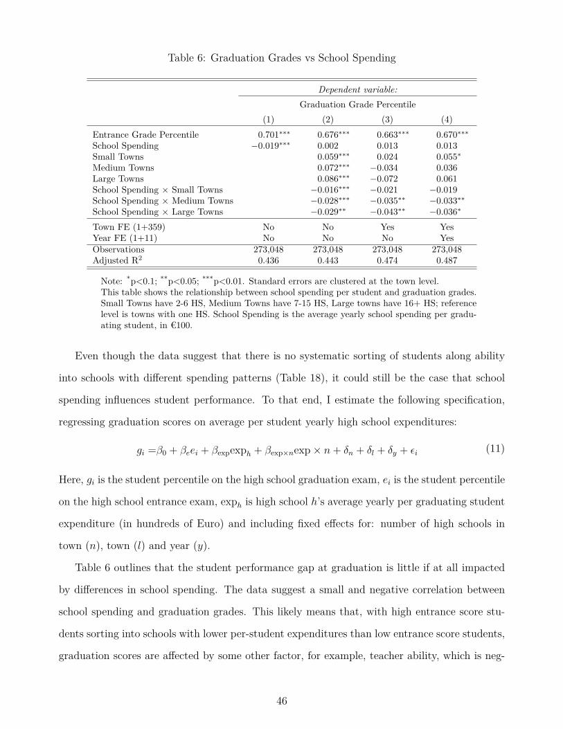
Table 6: Graduation Grades vs School Spending

Dependent variable:Graduation Grade Percentile

(1) (2) (3) (4)Entrance Grade Percentile 0.701∗∗∗ 0.676∗∗∗ 0.663∗∗∗ 0.670∗∗∗School Spending −0.019∗∗∗ 0.002 0.013 0.013Small Towns 0.059∗∗∗ 0.024 0.055∗Medium Towns 0.072∗∗∗ −0.034 0.036Large Towns 0.086∗∗∗ −0.072 0.061School Spending × Small Towns −0.016∗∗∗ −0.021 −0.019School Spending × Medium Towns −0.028∗∗∗ −0.035∗∗ −0.033∗∗School Spending × Large Towns −0.029∗∗ −0.043∗∗ −0.036∗

Town FE (1+359) No No Yes YesYear FE (1+11) No No No YesObservations 273,048 273,048 273,048 273,048Adjusted R2 0.436 0.443 0.474 0.487

Note: *p<0.1; **p<0.05; ***p<0.01. Standard errors are clustered at the town level.This table shows the relationship between school spending per student and graduation grades.Small Towns have 2-6 HS, Medium Towns have 7-15 HS, Large towns have 16+ HS; referencelevel is towns with one HS. School Spending is the average yearly school spending per gradu-ating student, in €100.

Even though the data suggest that there is no systematic sorting of students along ability

into schools with different spending patterns (Table 18), it could still be the case that school

spending influences student performance. To that end, I estimate the following specification,

regressing graduation scores on average per student yearly high school expenditures:

gi =β0 + βeei + βexpexph + βexp×nexp× n+ δn + δl + δy + εi (11)

Here, gi is the student percentile on the high school graduation exam, ei is the student percentile

on the high school entrance exam, exph is high school h’s average yearly per graduating student

expenditure (in hundreds of Euro) and including fixed effects for: number of high schools in

town (n), town (l) and year (y).

Table 6 outlines that the student performance gap at graduation is little if at all impacted

by differences in school spending. The data suggest a small and negative correlation between

school spending and graduation grades. This likely means that, with high entrance score stu-

dents sorting into schools with lower per-student expenditures than low entrance score students,

graduation scores are affected by some other factor, for example, teacher ability, which is neg-

46

atively correlated with school expenditures.

Note that school expenditures here exclude staff wages and represent a flow variable that

may be uninformative of the infrastructure stock accumulated in a school. In that sense, if

schools with an infrastructure deficit are more likely to spend more money in order to close

this gap, the results in Table 6 can be consistent with infrastructure having a positive effect on

grades and driving some of the observed graduation grade gap. Unfortunately, data on material

school stock is not available.

5.3 Decomposing Sorting Effects

I explored the relationship between peer effects, school spending, teacher ability and graduation

grades. The evidence suggests that teacher and peer abilities are associated with better educa-

tional outcomes and may widen performance gaps. On the other hand, peer effects and school

expenditures seem to have a much smaller, if any, impact on school performance. I now provide

a simple model explaining each of these three channels’ relative importance in explaining the

effect of student sorting on performance. I use the following baseline model:

gi = β0 + βeei + βµµ̂e-ih + δn + δd + δy + δl + εi (12)

Here, gi is the student percentile on the high school graduation exam, ei is the student percentile

on the high school entrance exam and µe−ih is the mean entrance exam grade in high school h,

excluding student i.38 Fixed effects are denoted by δ and include the following: δd (town-cohort

entrance grade decile of student i), δn (number of high schools in town), δy (year) and town

(δl).

I instrument µ̂eh, using the relative rank of a student within their town (dly(ei)), interacted

with the number of high schools in that town (nly):

µhy = γ0 + γeei + ηn + ηd + ηd×n + ηy + ηl + ξi (13)

This baseline specification is then sequentially augmented to include measures of high school-

38Note that this is slightly different than the specification in Equation 3. In that model, I used high school-yearentrance grade averages (µe−ihy) as a proxy of school quality. Here, I am using high school entrance gradeaverages. The reason is that I want to use yearly changes in cohort ability to identify peer effects, while thetime-invariant average is used to proxy school quality over the entire sample period.

47

level teacher ability (µthy), school expenditures per student (exph) and peer ability (more specif-

ically, the yearly deviation from the mean in peer entrance scores, µhy(ei)− µh(ei)):

gi =β0 + βeei + βµµ̂eh + δn + δdl(ei) + δy + δl+

βtµthy + βexpexph + βpeer(µhy(ei)− µh(ei)) + εi

(14)

After adding teacher, expenditure and peer variables, we can observe how the coefficient of

interest βµ changes. If this coefficient shrinks to the point of becoming insignificant, it is

possible to conclude that the three channels we consider explain most of the sorting effects on

graduation grades. Moreover, by adding the variables to the model one by one and observing

the impact on βµ, I can quantify the relative impact of each channel in explaining the effects of

sorting.

Table 7: Decomposition of Sorting Effects (Second Stage)

Dependent variable:Graduation Exam Component Percentile

(Baseline) (Peers) (Teachers) (Exp) (P+T) (P+T+E)Adm. Score Percentile (Ro) 0.155∗∗∗ 0.145∗∗∗ 0.158∗∗∗ 0.155∗∗∗ 0.147∗∗∗ 0.147∗∗∗

Adm. Score Percentile (Math) 0.070∗∗∗ 0.059∗∗∗ 0.076∗∗∗ 0.070∗∗∗ 0.070∗∗∗ 0.063∗∗∗

Peers (School) −0.178∗∗∗ −0.178∗∗∗ −0.185∗∗∗

Teacher 0.097∗∗∗ 0.097∗∗∗ 0.096∗∗∗

Expenditure −0.001 −0.002∗

Instrumented Peer Adm. Score (School) 0.063∗ 0.048 0.028 0.060∗ 0.013 0.009Number of High Schools in Town 4 4 4 4 4 4Town-Cohort Adm. Score Decile (d) 10 10 10 10 10 10N. Students Cohort (Town-Year) Yes Yes Yes Yes Yes YesN. Students Cohort (T-Y) × d Yes Yes Yes Yes Yes YesTown Unemployment Level Yes Yes Yes Yes Yes YesCounty HS Dropout Rate Yes Yes Yes Yes Yes YesCounty Average Wage Yes Yes Yes Yes Yes YesTown FE 337 337 337 337 337 337Year FE 5 5 5 5 5 5

Note: *p<0.1; **p<0.05; ***p<0.01. Standard errors are clustered at the town level.This table shows estimation results of Equation 14. It shows the relationship between graduationexam subject scores (e.g. math, Romanian) and school quality, proxied by average admission scores,conditional on own entrance grade. Each column represents a specification in which I add peer effects,teacher ability and/or school expenditure to the baseline model. Number of high schools are groupedinto four bins. Town-cohort admissions core deciles (d) are student entrance exam deciles within theirtown and cohort; reference level is the bottom entrance grade decile (d1). Peer quality is identifiedby the differences in within-school average admission scores from year to year. Teacher ability is theaverage placement test percentile of teacher who worked during a student’s four year stay, weightedby the number of weekly hours worked. Since I look at graduation exam components separately,onlyteachers teaching relevant subjects are included on the righ-hand side (e.g. math and physicsteachers for science component grades). Expenditures are measured in hundreds of Euro/student/year.Peer admission scores are instrumented by an interaction of town-cohort admission deciles and thenumber of high schools within a town.

Table 7 presents the results of this decomposition. The baseline specification shows that

48

going to a school with a one percentage point higher average entrance grade causes a 0.069

percentile increase in graduation grade.39 A similar specification at the track-level is estimated

in Table 22.

I find that the three channels explored in this paper explain 78% (83%) of the effects of

attending a better high school (track). Using a Gelbach decomposition,40 I find that at the

high school level, differences in teacher ability, peer effects and school spending account for

62%, 32% and 6%, respectively of the explained component. As much as 84% of the explained

variation is accounted for by differences in teacher ability at the track level. These two findings

imply that, within high schools, there are significant track-level differences in teacher ability.

Meanwhile, peer effects and school expenditures only account for 7% and 9% of track-level

explained variation.

It is plausible that the estimates for teacher ability’s relative contribution are relatively

conservative for two reasons. First of all, the teacher data is quite noisy and only captures new

hires, of which many are temporary teachers. There is no information on the variation of the

abilities of existing teachers within a school. Second, and perhaps more importantly, the data

does not allow the matching of students to teachers. As such, the variation in teacher ability is

at the school-year level. I expect the hiring of a new teacher to have a relatively small impact

on the average student’s graduation grade in a school. Indeed, this teacher will only be matched

to some classes of the four grades in a high school.

Thus, the decomposition shows that student sorting affects performance mainly by creating

inequalities in access to competent teachers. While peer effects and school expenditures do seem

to play a role, their contribution is dwarfed by that of teachers.

39This is different from the IV specification results for several reasons. First of all, the sample used here isrestricted to the students who have matching teachers and school expenditures. Moreover, the school qualityproxy used in the present specification is the mean entrance score of student within the school, rather thanthe mean in the year a student was admitted. This is because I want to use the yearly variation in cohortability to identify peer effects. Lastly, graduation and entrance scores are broken down by subject componentto match the data to the teacher data, which is subject-specific.

40Intuitively, this decomposition is not sensitive to the order in which we add the explanatory variables to thefull model and capturing variance and covariance structures of the variables of interest. For more details,consult Gelbach (2016).

49

6 Discussion and Conclusion

This paper investigates the effects of student sorting along ability on educational outcomes.

The competitive high school admission system in Romania gives rise to very extreme sorting

patterns that display significant and systematic geographic variation that can be used to identify

the effects of sorting on student outcomes. Moreover, student admission and graduation records

are matched to teacher ability and school expenditure data for the first time, which allows the

exploration of the different channels through which sorting impacts school performance.

I first document how students sort in schools and how this sorting affects student grades.

I find that sorting markedly increases in the number of high school choices available to stu-

dents. As the number of local high schools increases, segregation of students across ability rises

markedly and there is a widening the performance gap between high-ability and low-ability

students. Thus, the data paint a stark picture when it comes to school choice policies: increases

in school choices exacerbate educational inequalities.

Second, I decompose the channels through which sorting impacts school outcomes. While

peer effects are not, on average, significant, there is significant heterogeneity: high entrance score

students within tracks or schools benefit from having better peers, while this is detrimental to

low entrance score students.

I also show that teacher sorting closely mirrors student sorting, such that high-ability stu-

dents are more likely to attend schools where high-ability teachers work. This happens in two

ways: high-ability teachers are more likely to work in bigger cities and, within cities, high-

ability teachers are more likely to find teaching positions in schools attended by high-ability

students. This occurs despite the fact that teacher salaries do not vary by school or town in

this educational system. By exploiting between-school variation in the quality of teaching bod-

ies, conditional on student abilities, I find that high-ability teachers add value. Moreover, I

find evidence that high-ability students benefit from high-ability teachers more than low-ability

students.

To conclude, the results suggest that the main channel through which sorting increases

inequality is access to high-ability teachers. A higher degree of school choice leads to a high

50

entrance score students gaining access to higher ability teachers than their low entrance score

counterparts. Moreover, peer and teacher ability results suggest that there are tradeoffs in terms

of policy. Policymakers may reduce inequalities in education by either reducing the extent of

student sorting41 or by assigning high-ability teachers to low-ability students. However, doing

this comes with an efficiency loss. There are performance complementarities to be obtained both

by grouping high-ability students and assigning high-ability teachers to high-ability students.

Lastly, there is also a policy implication about school construction. While Duflo (2001)

suggests that school openings have strong and persistent effects on average educational outcomes

and wages, the Romanian data suggest that, at least in a context in which there is school choice,

high-ability students are the main beneficiaries. Meanwhile, low-ability students may actually

be negatively impacted by school construction. Overall, there is evidence that a new school

opening in a location negatively affects average student scores while also increasing inequality.

41For example, by randomly assigning students to schools.

51

References

Joshua D Angrist. The perils of peer effects. Labour Economics, 30:98–108, 2014.

Joshua D Angrist, Susan M Dynarski, Thomas J Kane, Parag A Pathak, and Christopher R

Walters. Who benefits from kipp? Journal of policy Analysis and Management, 31(4):

837–860, 2012.

Abhijit V Banerjee, Shawn Cole, Esther Duflo, and Leigh Linden. Remedying education: Evi-

dence from two randomized experiments in india. The Quarterly Journal of Economics, 122

(3):1235–1264, 2007.

Mary A Burke and Tim R Sass. Classroom peer effects and student achievement. Journal of

Labor Economics, 31(1):51–82, 2013.

Scott E Carrell, Mark Hoekstra, and Elira Kuka. The long-run effects of disruptive peers.

American Economic Review, 108(11):3377–3415, 2018.

Raj Chetty, John N Friedman, Nathaniel Hilger, Emmanuel Saez, Diane Whitmore Schanzen-

bach, and Danny Yagan. How does your kindergarten classroom affect your earnings? evi-

dence from project star. The Quarterly journal of economics, 126(4):1593–1660, 2011.

Raj Chetty, John N Friedman, and Jonah E Rockoff. Measuring the impacts of teachers i:

Evaluating bias in teacher value-added estimates. American Economic Review, 104(9):2593–

2632, 2014.

Anna K Chmielewski. An international comparison of achievement inequality in within-and

between-school tracking systems. American Journal of Education, 120(3):293–324, 2014.

Courtney A Collins and Li Gan. Does sorting students improve scores? an analysis of class

composition. Technical report, National Bureau of Economic Research, 2013.

Diana Coman. Bac data. http://ossasepia.com/bac-data, 2020. Accessed: 2020-03-20.

52

Will Dobbie and Roland G Fryer Jr. Are high-quality schools enough to increase achievement

among the poor? evidence from the harlem children’s zone. American Economic Journal:

Applied Economics, 3(3):158–87, 2011.

Will Dobbie and Roland G Fryer Jr. Getting beneath the veil of effective schools: Evidence

from new york city. American Economic Journal: Applied Economics, 5(4):28–60, 2013.

Esther Duflo. Schooling and labor market consequences of school construction in indonesia:

Evidence from an unusual policy experiment. American economic review, 91(4):795–813,

2001.

Esther Duflo, Pascaline Dupas, and Michael Kremer. Peer effects, teacher incentives, and the

impact of tracking: Evidence from a randomized evaluation in kenya. American Economic

Review, 101(5):1739–74, 2011.

David N Figlio and Marianne E Page. School choice and the distributional effects of ability

tracking: does separation increase inequality? Journal of Urban Economics, 51(3):497–514,

2002.

Jonah B Gelbach. When do covariates matter? and which ones, and how much? Journal of

Labor Economics, 34(2):509–543, 2016.

Eric A Hanushek and Ludger Wößmann. Does educational tracking affect performance and

inequality? differences-in-differences evidence across countries. The Economic Journal, 116

(510):C63–C76, 2006.

Eric A Hanushek, John F Kain, Daniel M O’Brien, and Steven G Rivkin. The market for

teacher quality. Technical report, National Bureau of Economic Research, 2005.

Caroline M Hoxby. School choice and school productivity: Could school choice be a tide that

lifts all boats? In The economics of school choice, pages 287–342. University of Chicago

Press, 2007.

53

Scott A Imberman. The effect of charter schools on achievement and behavior of public school

students. Journal of Public Economics, 95(7-8):850–863, 2011.

C Kirabo Jackson. What do test scores miss? the importance of teacher effects on non–test

score outcomes. Journal of Political Economy, 126(5):2072–2107, 2018.

Maciej Jakubowski, Harry Anthony Patrinos, Emilio Ernesto Porta, and Jerzy Wiśniewski. The

effects of delaying tracking in secondary school: evidence from the 1999 education reform in

poland. Education Economics, 24(6):557–572, 2016.

David L Lee, Justin McCrary, Marcelo J Moreira, and Jack Porter. Valid t-ratio inference for

iv. arXiv preprint arXiv:2010.05058, 2020.

Ofer Malamud and Cristian Pop-Eleches. School tracking and access to higher education among

disadvantaged groups. Journal of Public Economics, 95(11-12):1538–1549, 2011.

Charles F Manski. Identification of endogenous social effects: The reflection problem. The

review of economic studies, 60(3):531–542, 1993.

Eleonora Patacchini, Edoardo Rainone, and Yves Zenou. Heterogeneous peer effects in educa-

tion. Journal of Economic Behavior & Organization, 134:190–227, 2017.

Nathan Petek and Nolan Pope. The multidimensional impact of teachers on students. Technical

report, University of Chicago Working Paper, 2016.

Cristian Pop-Eleches and Miguel Urquiola. Going to a better school: Effects and behavioral

responses. American Economic Review, 103(4):1289–1324, 2013.

Steven G Rivkin, Eric A Hanushek, and John F Kain. Teachers, schools, and academic achieve-

ment. Econometrica, 73(2):417–458, 2005.

Jonah E Rockoff. The impact of individual teachers on student achievement: Evidence from

panel data. American economic review, 94(2):247–252, 2004.

Bruce Sacerdote. Peer effects with random assignment: Results for dartmouth roommates. The

Quarterly Journal of Economics, 116(2):681–704, 2001.

54

Bruce Sacerdote. Peer effects in education: How might they work, how big are they and how

much do we know thus far? In Handbook of the Economics of Education, volume 3, pages

249–277. Elsevier, 2011.

James H Stock and Motohiro Yogo. Testing for weak instruments in linear iv regression. Tech-

nical report, National Bureau of Economic Research, 2002.

Jeffrey M Wooldridge. Econometric analysis of cross section and panel data mit press. Cam-

bridge, MA, 108:146–151, 2002.

55

Appendices

A Tables, Figures and Regression Results

Table 8: Regression of Graduation Grade vs Entrance Grade, by Town Size

Dependent variable:Graduation Grade Percentile

(1) (2) (3) (4) (5) (6)Entrance Grade Percentile 0.710∗∗∗ 0.582∗∗∗ 0.631∗∗∗ 0.571∗∗∗ 0.563∗∗∗ 0.644∗∗∗

d2 × n2-6 −0.015∗∗ −0.013∗ −0.010 −0.014∗∗ −0.014∗∗ −0.015∗∗

d3 × n2-6 −0.014∗ −0.009 −0.005 −0.015∗∗ −0.016∗∗ −0.020∗∗∗

d4 × n2-6 −0.011 −0.002 0.004 −0.015∗ −0.016∗∗ −0.022∗∗∗

d5 × n2-6 0.0001 0.011 0.018∗∗ −0.011 −0.010 −0.018∗∗

d6 × n2-6 0.018∗ 0.031∗∗ 0.037∗∗∗ 0.001 0.003 −0.006d7 × n2-6 0.029∗∗∗ 0.043∗∗∗ 0.048∗∗∗ 0.008 0.009 −0.001d8 × n2-6 0.030∗∗∗ 0.044∗∗∗ 0.049∗∗∗ 0.012 0.013 0.002d9 × n2-6 0.042∗∗∗ 0.055∗∗∗ 0.059∗∗∗ 0.025∗∗ 0.024∗∗ 0.014d10 × n2-6 0.054∗∗∗ 0.060∗∗∗ 0.064∗∗∗ 0.036∗∗∗ 0.030∗∗∗ 0.023∗∗

d2 × n7-15 −0.026∗∗∗ −0.023∗∗ −0.017∗ −0.019∗∗ −0.021∗∗ −0.023∗∗∗

d3 × n7-15 −0.031∗∗ −0.022 −0.015 −0.018 −0.019∗ −0.025∗∗

d4 × n7-15 −0.016 −0.003 0.005 −0.007 −0.008 −0.018d5 × n7-15 0.009 0.026 0.032∗∗ 0.008 0.008 −0.004d6 × n7-15 0.040∗∗∗ 0.058∗∗∗ 0.063∗∗∗ 0.030∗ 0.028∗∗ 0.015d7 × n7-15 0.059∗∗∗ 0.079∗∗∗ 0.081∗∗∗ 0.040∗∗∗ 0.038∗∗∗ 0.023∗

d8 × n7-15 0.066∗∗∗ 0.087∗∗∗ 0.088∗∗∗ 0.047∗∗∗ 0.044∗∗∗ 0.028∗∗

d9 × n7-15 0.075∗∗∗ 0.094∗∗∗ 0.094∗∗∗ 0.055∗∗∗ 0.049∗∗∗ 0.034∗∗

d10 × n7-15 0.082∗∗∗ 0.092∗∗∗ 0.094∗∗∗ 0.058∗∗∗ 0.048∗∗∗ 0.038∗∗∗

d2 × n16+ −0.014∗ −0.006 0.0004 −0.0004 −0.002 −0.004d3 × n16+ −0.008 0.007 0.015 0.013 0.009 0.002d4 × n16+ 0.003 0.023 0.032∗∗∗ 0.026∗∗ 0.021∗∗ 0.009d5 × n16+ 0.031∗∗ 0.055∗∗∗ 0.063∗∗∗ 0.043∗∗∗ 0.039∗∗∗ 0.025∗∗

d6 × n16+ 0.056∗∗∗ 0.082∗∗∗ 0.088∗∗∗ 0.055∗∗∗ 0.051∗∗∗ 0.035∗∗∗

d7 × n16+ 0.070∗∗∗ 0.098∗∗∗ 0.101∗∗∗ 0.063∗∗∗ 0.058∗∗∗ 0.041∗∗∗

d8 × n16+ 0.074∗∗∗ 0.102∗∗∗ 0.105∗∗∗ 0.068∗∗∗ 0.062∗∗∗ 0.044∗∗∗

d9 × n16+ 0.087∗∗∗ 0.112∗∗∗ 0.114∗∗∗ 0.080∗∗∗ 0.071∗∗∗ 0.055∗∗∗

d10 × n16+ 0.096∗∗∗ 0.110∗∗∗ 0.115∗∗∗ 0.084∗∗∗ 0.072∗∗∗ 0.061∗∗∗

Entrance Grade Decile (1+9) Yes Yes Yes Yes Yes YesN HS Students (Town) Yes Yes Yes Yes Yes YesN HS Students (Town) × Yes Yes Yes Yes Yes YesEntrance Grade DecileN HS Town (1+4) Yes Yes Yes Yes Yes YesTown FE (1+537) No Yes Yes Yes Yes NoYear FE (1+11) No No Yes Yes Yes YesTrack FE (1+116) No No No Yes Yes YesMS FE (1+19,271) No No No No Yes YesObservations 1,170,680 1,170,680 1,170,680 1,170,680 1,170,680 1,170,680Adjusted R2 0.518 0.539 0.568 0.599 0.635 0.633

Note: *p<0.1; **p<0.05; ***p<0.01. Standard errors are clustered at the county level.This table shows the estimation results of Equation 2, where d is the entrance grade decile (at the town-cohort level) and nis the number of high schools in a town.

56

Table 9: Student vs High School Peers Entrance Grades

Student Entrance GradePercentile

d2 0.013***

d3 0.023***

d4 0.031***

d5 0.037***

d6 0.042***

d7 0.046***

d8 0.050***

d9 0.054***

d10 0.060***

Small Towns −0.236***

Medium Towns −0.257***

Large Towns −0.273***

d2 × Small Towns 0.024***

d3 × Small Towns 0.059***

d4 × Small Towns 0.106***

d5 × Small Towns 0.167***

d6 × Small Towns 0.235***

d7 × Small Towns 0.303***

d8 × Small Towns 0.356***

d9 × Small Towns 0.392***

d10 × Small Towns 0.419***

d2 × Medium Towns 0.014***

d3 × Medium Towns 0.039***

d4 × Medium Towns 0.077***

d5 × Medium Towns 0.141***

d6 × Medium Towns 0.226***

d7 × Medium Towns 0.325***

d8 × Medium Towns 0.422***

d9 × Medium Towns 0.489***

d10 × Medium Towns 0.530***

d2 × Large Towns 0.008***

d3 × Large Towns 0.036***

d4 × Large Towns 0.086***

d5 × Large Towns 0.153***

d6 × Large Towns 0.248***

d7 × Large Towns 0.351***

d8 × Large Towns 0.443***

d9 × Large Towns 0.528***

d10 × Large Towns 0.600***

Town FE (1+554) YesYear FE (1+11) YesObservations 1,843,891Adjusted R2 0.766

Note: *p<0.1; **p<0.05; ***p<0.01.This table shows the relationship between astudent’s entrance grade and their high schoolpeer’s average entrance grade.Small Towns have 2-6 HS, Medium Townshave 7-15 HS, Large towns have 16+ HS; ref-erence level is towns with one high school.Deciles (d) are student entrance grade decileswithin their cohort (nationallu); referencelevel is the bottom entrance grade decile (d1).

57

Table 10: IV First Stage (School)

Dependent variable:Average Peer Exam Score Percentile(1) (2) (3)

Admission Score (Percentile) 0.662∗∗∗ 0.285∗∗∗ 0.269∗∗∗

d2 × n2 −0.001 −0.002 −0.001d3 × n2 0.011 0.009 0.010d4 × n2 0.032∗∗ 0.029∗∗∗ 0.031∗∗∗

d5 × n2 0.063∗∗∗ 0.053∗∗∗ 0.055∗∗∗

d6 × n2 0.099∗∗∗ 0.086∗∗∗ 0.089∗∗∗

d7 × n2 0.126∗∗∗ 0.110∗∗∗ 0.112∗∗∗

d8 × n2 0.139∗∗∗ 0.123∗∗∗ 0.125∗∗∗

d9 × n2 0.146∗∗∗ 0.132∗∗∗ 0.134∗∗∗

d10 × n2 0.163∗∗∗ 0.143∗∗∗ 0.144∗∗∗

d2 × n3 0.001 0.008 0.010d3 × n3 0.008 0.014 0.019∗

d4 × n3 0.023 0.028∗ 0.037∗∗∗

d5 × n3 0.053∗∗ 0.052∗∗∗ 0.065∗∗∗

d6 × n3 0.105∗∗∗ 0.097∗∗∗ 0.113∗∗∗

d7 × n3 0.157∗∗∗ 0.141∗∗∗ 0.154∗∗∗

d8 × n3 0.199∗∗∗ 0.179∗∗∗ 0.187∗∗∗

d9 × n3 0.224∗∗∗ 0.203∗∗∗ 0.208∗∗∗

d10 × n3 0.261∗∗∗ 0.226∗∗∗ 0.226∗∗∗

d2 × n4-15 0.001 0.010∗∗ 0.012∗∗

d3 × n4-15 0.019∗ 0.033∗∗∗ 0.040∗∗∗

d4 × n4-15 0.050∗∗∗ 0.064∗∗∗ 0.075∗∗∗

d5 × n4-15 0.102∗∗∗ 0.111∗∗∗ 0.124∗∗∗

d6 × n4-15 0.163∗∗∗ 0.169∗∗∗ 0.184∗∗∗

d7 × n4-15 0.237∗∗∗ 0.235∗∗∗ 0.247∗∗∗

d8 × n4-15 0.301∗∗∗ 0.290∗∗∗ 0.297∗∗∗

d9 × n4-15 0.352∗∗∗ 0.335∗∗∗ 0.337∗∗∗

d10 × n4-15 0.411∗∗∗ 0.370∗∗∗ 0.367∗∗∗

d2 × n16+ −0.006 0.010∗∗ 0.011d3 × n16+ 0.017 0.040∗∗∗ 0.045∗∗∗

d4 × n16+ 0.056∗∗∗ 0.080∗∗∗ 0.089∗∗∗

d5 × n16+ 0.117∗∗∗ 0.138∗∗∗ 0.141∗∗∗

d6 × n16+ 0.196∗∗∗ 0.211∗∗∗ 0.208∗∗∗

d7 × n16+ 0.274∗∗∗ 0.287∗∗∗ 0.273∗∗∗

d8 × n16+ 0.348∗∗∗ 0.353∗∗∗ 0.333∗∗∗

d9 × n16+ 0.424∗∗∗ 0.416∗∗∗ 0.390∗∗∗

d10 × n16+ 0.520∗∗∗ 0.481∗∗∗ 0.437∗∗∗

Number of High Schools in Town 4 4 4Town-Cohort Admission Score Decile (d) No Yes YesNumber of Students (Town-Cohort) No No YesNumber of Students (Town-Cohort) × d No No YesTown Unemployment Level No No YesTown Unemployment Level × d No No YesCounty HS Dropout Rate No No YesCounty HS Dropout Rate × d No No YesCounty Average Wage No No YesCounty Average Wage × d No No YesTown FE No 552 544Year FE No 12 12Track FE No 191 191MS FE No 18,921 18,590Observations 1,180,088 1,180,088 1,161,360Adjusted R2 0.717 0.823 0.827Weak Instrument Test p-value 0 0 0Wu-Hausman p-value 0 0.54 0

Note: *p<0.1; **p<0.05; ***p<0.01. Standard errors are clusteredat the county level.This table shows first stage results form the equation 3. Peer admis-sion scores (at the school level) are instrumented using an interac-tion between student’s own admission score decile and the number ofhigh schools int he town in which they attend high school. Controlsinclude the number of high schools in town (grouped into 4 bins),within town-cohort own admission score decile, number of studentsadmitted in towns in a given year, town unemployment level andcounty high school dropout levels and average wage levels (all com-puted as averages of 2010-2019 yearly data), town fixed effects, yearfixed effects, track type fixed effects and middle school fixed effects.

58

Table 11: IV First Stage (Track)

Dependent variable:Average Peer Exam Score Percentile(1) (2) (3)

Admission Score (Percentile) 0.698∗∗∗ 0.370∗∗∗ 0.358∗∗∗

d2 × n2 0.008 0.006 0.007d3 × n2 0.014∗ 0.010∗ 0.011∗

d4 × n2 0.022∗∗ 0.017∗∗ 0.018∗∗

d5 × n2 0.034∗∗∗ 0.022∗∗∗ 0.023∗∗∗

d6 × n2 0.046∗∗∗ 0.032∗∗∗ 0.033∗∗∗

d7 × n2 0.051∗∗∗ 0.037∗∗∗ 0.039∗∗∗

d8 × n2 0.053∗∗∗ 0.042∗∗∗ 0.044∗∗∗

d9 × n2 0.062∗∗∗ 0.051∗∗∗ 0.053∗∗∗

d10 × n2 0.083∗∗∗ 0.062∗∗∗ 0.064∗∗∗

d2 × n3 0.001 0.005 0.006d3 × n3 0.007 0.008 0.012d4 × n3 0.013 0.012 0.019d5 × n3 0.021 0.014 0.021∗

d6 × n3 0.042∗∗ 0.029∗∗ 0.037∗∗∗

d7 × n3 0.061∗∗∗ 0.046∗∗∗ 0.053∗∗∗

d8 × n3 0.078∗∗∗ 0.062∗∗∗ 0.065∗∗∗

d9 × n3 0.093∗∗∗ 0.077∗∗∗ 0.077∗∗∗

d10 × n3 0.126∗∗∗ 0.095∗∗∗ 0.093∗∗∗

d2 × n4-15 0.004 0.008∗ 0.009∗

d3 × n4-15 0.011 0.019∗∗∗ 0.025∗∗∗

d4 × n4-15 0.023∗ 0.029∗∗∗ 0.038∗∗∗

d5 × n4-15 0.046∗∗∗ 0.046∗∗∗ 0.055∗∗∗

d6 × n4-15 0.067∗∗∗ 0.067∗∗∗ 0.077∗∗∗

d7 × n4-15 0.097∗∗∗ 0.093∗∗∗ 0.101∗∗∗

d8 × n4-15 0.124∗∗∗ 0.118∗∗∗ 0.122∗∗∗

d9 × n4-15 0.154∗∗∗ 0.145∗∗∗ 0.144∗∗∗

d10 × n4-15 0.206∗∗∗ 0.175∗∗∗ 0.169∗∗∗

d2 × n16+ 0.000 0.007 0.010d3 × n16+ 0.012 0.022∗∗∗ 0.033∗∗∗

d4 × n16+ 0.029∗ 0.038∗∗∗ 0.054∗∗∗

d5 × n16+ 0.054∗∗∗ 0.058∗∗∗ 0.070∗∗∗

d6 × n16+ 0.089∗∗∗ 0.086∗∗∗ 0.091∗∗∗

d7 × n16+ 0.122∗∗∗ 0.122∗∗∗ 0.119∗∗∗

d8 × n16+ 0.158∗∗∗ 0.158∗∗∗ 0.149∗∗∗

d9 × n16+ 0.204∗∗∗ 0.198∗∗∗ 0.184∗∗∗

d10 × n16+ 0.284∗∗∗ 0.248∗∗∗ 0.217∗∗∗

Number of High Schools in Town 4 4 4Town-Cohort Admission Score Decile (d) No Yes YesNumber of Students (Town-Cohort) No No YesNumber of Students (Town-Cohort) × d No No YesTown Unemployment Level No No YesTown Unemployment Level × d No No YesCounty HS Dropout Rate No No YesCounty HS Dropout Rate × d No No YesCounty Average Wage No No YesCounty Average Wage × d No No YesTown FE No 552 544Year FE No 12 12Track FE No 191 191MS FE No 18,592 18,590Observations 1,179,769 1,179,769 1,161,051Adjusted R2 0.753 0.860 0.860Weak Instrument Test p-value 0 0 0Wu-Hausman p-value 0 0 0

Note: *p<0.1; **p<0.05; ***p<0.01. Standard errors are clusteredat the county level.This table shows first stage results form the equation 3. Peer admis-sion scores (at the track level) are instrumented using an interactionbetween student’s own admission score decile and the number ofhigh schools int he town in which they attend high school. Controlsinclude the number of high schools in town (grouped into 4 bins),within town-cohort own admission score decile, number of studentsadmitted in towns in a given year, town unemployment level andcounty high school dropout levels and average wage levels (all com-puted as averages of 2010-2019 yearly data), town fixed effects, yearfixed effects, track type fixed effects and middle school fixed effects.

59

Table 12: IV Second Stage (School)

Dependent variable:Graduation Exam Score Percentile(1) (2) (3)

Admission Score (Percentile) 0.590∗∗∗ 0.566∗∗∗ 0.530∗∗∗Instrumented Peer Admission Score (Percentile) 0.367∗∗∗ 0.322∗∗∗ 0.356∗∗∗

Number of High Schools in Town 4 4 4Town-Cohort Admission Score Decile (d) No Yes YesNumber of Students (Town-Cohort) No No YesNumber of Students (Town-Cohort) × d No No YesTown Unemployment Level No No YesTown Unemployment Level × d No No YesCounty HS Dropout Rate No No YesCounty HS Dropout Rate × d No No YesCounty Average Wage No No YesCounty Average Wage × d No No YesTown FE No 552 544Year FE No 12 12Track FE No 191 191MS FE No 18,592 18,590Observations 1,180,088 1,180,088 1,161,360Adjusted R2 0.638 0.638 0.639

Note: *p<0.1; **p<0.05; ***p<0.01. Standard errors are clustered at the county level.This table shows second stage results form the equation 3. Student graduation exams scores(in percentiles at the cohort-country level) are regressed on similar admission scores and peeradmission scores. Peer admission scores (at the track level) are instrumented using an interactionbetween student’s own admission score decile and the number of high schools int he town in whichthey attend high school. Controls include the number of high schools in town (grouped into 4bins), within town-cohort own admission score decile, number of students admitted in towns ina given year, town unemployment level and county high school dropout levels and average wagelevels (all computed as averages of 2010-2019 yearly data), town fixed effects, year fixed effects,track type fixed effects and middle school fixed effects.

60

Table 13: IV Second Stage (Track)

Dependent variable:Graduation Exam Score Percentile(1) (2) (3)

Admission Score (Percentile) 0.486∗∗∗ 0.521∗∗∗ 0.454∗∗∗Instrumented Peer Admission Score (Percentile) 0.341∗∗∗ 0.246∗∗∗ 0.353∗∗∗

Number of High Schools in Town 4 4 4Town-Cohort Admission Score Decile (d) No Yes YesNumber of Students (Town-Cohort) No No YesNumber of Students (Town-Cohort) × d No No YesTown Unemployment Level No No YesTown Unemployment Level × d No No YesCounty HS Dropout Rate No No YesCounty HS Dropout Rate × d No No YesCounty Average Wage No No YesCounty Average Wage × d No No YesTown FE No 552 544Year FE No 12 12Track FE No 191 191MS FE No 18,592 18,590Observations 1,179,769 1,179,769 1,161,051Adjusted R2 0.533 0.638 0.638

Note: *p<0.1; **p<0.05; ***p<0.01. Standard errors are clustered at the county level.This table shows second stage results form the equation 3. Student graduation exams scores(in percentiles at the cohort-country level) are regressed on similar admission scores and peeradmission scores. Peer admission scores (at the track level) are instrumented using an interactionbetween student’s own admission score decile and the number of high schools int he town in whichthey attend high school. Controls include the number of high schools in town (grouped into 4bins), within town-cohort own admission score decile, number of students admitted in towns ina given year, town unemployment level and county high school dropout levels and average wagelevels (all computed as averages of 2010-2019 yearly data), town fixed effects, year fixed effects,track type fixed effects and middle school fixed effects.

61

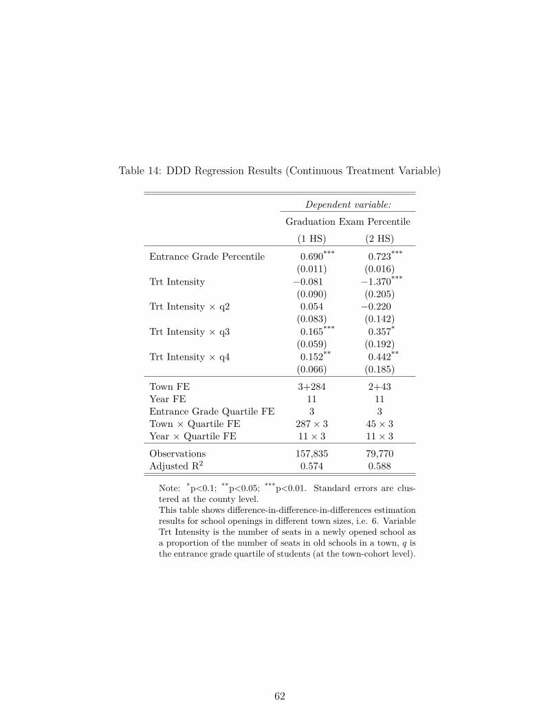
Table 14: DDD Regression Results (Continuous Treatment Variable)

Dependent variable:Graduation Exam Percentile

(1 HS) (2 HS)

Entrance Grade Percentile 0.690*** 0.723***(0.011) (0.016)

Trt Intensity −0.081 −1.370***(0.090) (0.205)

Trt Intensity × q2 0.054 −0.220(0.083) (0.142)

Trt Intensity × q3 0.165*** 0.357*(0.059) (0.192)

Trt Intensity × q4 0.152** 0.442**(0.066) (0.185)

Town FE 3+284 2+43Year FE 11 11Entrance Grade Quartile FE 3 3Town × Quartile FE 287× 3 45× 3Year × Quartile FE 11× 3 11× 3Observations 157,835 79,770Adjusted R2 0.574 0.588

Note: *p<0.1; **p<0.05; ***p<0.01. Standard errors are clus-tered at the county level.This table shows difference-in-difference-in-differences estimationresults for school openings in different town sizes, i.e. 6. VariableTrt Intensity is the number of seats in a newly opened school asa proportion of the number of seats in old schools in a town, q isthe entrance grade quartile of students (at the town-cohort level).

62

Table 15: List of HS Openings

Number of HS (before opening) Occurences First Full Cohort Graduation Year1 2 2012, 20172 1 2011

Note: This table contains information on the high school openings retained for the analysis.The “First Full Cohort Graduation Year” indicates the graduation year of the first studentsthat completed all four years in the newly opened high school.

Figure 13: DDD: Sorting Patterns Before and After School Opening (Control Group), byEntrance Score

Student in 90th Percentile Student in 99th Percentile

Student in 50th Percentile Student in 75th Percentile

Student in 10th Percentile Student in 25th Percentile

0.00 0.25 0.50 0.75 1.00 0.00 0.25 0.50 0.75 1.00

0

1

2

3

4

0

1

2

3

4

0

1

2

3

4

Entrance Grade (Percentile)

Den

sity Timing

After Opening

Before Opening

Note: This figure plots the distribution of student peers (within the same school) in thecontrol group, conditional on own entrance score, before and after high schools open inthe treatment group. Because the opening dates of high schools are staggered, I cannotdefine a unique “before” and “after” period for the control group. Instead, I use a “stackedcohort” approach: a different “before”/“after” dummy variable is created for the controlgroup based on each relevant high school opening year in the treatment group. This way,each high school opening has its corresponding control group with a well-defined perioddummy. The data is then “stacked” based on the period dummies.

63

Table 16: Teacher vs Coworkers Exam Grades

Teacher GradePercentile

q2 0.020**

q3 0.034***

q4 0.048***

Small Towns −0.007nMedium Towns 0.022Large Towns 0.056***

q2 × Small Towns 0.004q3 × Small Towns −0.006q4 × Small Towns 0.004q2 × Medium Towns 0.012q3 × Medium Towns 0.008q4 × Medium Towns 0.026q2 × Large Towns −0.002q3 × Large Towns 0.003q4 × Large Towns 0.017Subject FE (1+347) YesYear FE (1+4) YesObservations 18,634Adjusted R2 0.059

Note: *p<0.1; **p<0.05; ***p<0.01.This table shows the relationship be-tween a new teacher’s exam grade andtheir coworker’s average grade.Small Towns have 2-6 HS, MediumTowns have 7-15 HS, Large towns have16+ HS; reference level is towns withone high school. Quartiles (q) areteacher exam quartiles within theirsubject and cohort; reference level isthe bottom entrance grade quartile(q1).

64

Table 17: Teacher vs Student Exam Grades: Regression Results

Teacher GradePercentile

Entrance Grade Percentile 0.080***

q2 −0.018***

q3 −0.036***

q4 −0.055***

Small Towns −0.010***

Medium Towns −0.057***

Large Towns −0.056***

q2 × Small Towns 0.005***

q3 × Small Towns 0.004***

q4 × Small Towns 0.007***

q2 × Medium Towns 0.013***

q3 × Medium Towns 0.040***

q4 × Medium Towns 0.078***

q2 × Large Towns 0.008***

q3 × Large Towns 0.046***

q4 × Large Towns 0.094***

Subject FE (1+305) YesTown FE (1+529) YesYear FE (1+5) YesObservations 2,035,048Adjusted R2 0.258

Note: *p<0.1; **p<0.05; ***p<0.01.This table shows the relationship betweenstudent entrance scores and teachers work-ing in the same high school’s exam scores,by town size. Small Towns have 2-6 HS,Medium Towns have 7-15 HS, Large townshave 16+ HS; reference level is towns withone high school. Quartiles (q) are studententrance exam quartiles within their cohort;reference level is the bottom entrance gradequartile (q1).

65

Table 18: School Expenditure vs Entrance Grades

Dependent variable:Average School Expenditure per Student per Year (€)

Across Towns Within Towns(1) (2) (3) (4)

d2 −5.243*** −3.634∗∗∗ −5.260*** −3.876***

d3 −9.829*** −6.606*** −8.089*** −5.553***

d4 −13.590*** −8.498*** −10.105*** −6.930**

d5 −14.877*** −9.170*** −12.657*** −9.214***

d6 −16.045*** −10.320*** −14.596*** −11.885***

d7 −19.013*** −14.197*** −14.847*** −12.939***

d8 −19.692*** −15.765*** −16.042*** −14.326***

d9 −21.636*** −17.488*** −17.032*** −15.279***

d10 −24.773*** −19.487*** −18.227*** −16.135***

High School Cohort Size −10.114*** −8.550***

Town FE (1+359) No No Yes YesYear FE (1+11) Yes Yes Yes YesWithin-Town-Year Deciles No No Yes YesNational-Year Deciles No No Yes YesObservations 390,085 390,085 390,085 390,085Adjusted R2 0.205 0.232 0.419 0.428

Note: *p<0.1; **p<0.05; ***p<0.01. Standard errors are clustered at the county level.This table shows the relationship between per student school expenditures and studententrance scores. Reference level is students with first decile entrance scores. Deciles(d) are student entrance exam deciles (national, for columns 1 and 2, within cohort-town for column 3 and 4); reference level is the bottom entrance grade decile (d1).High school cohort sizes are standardized.

66

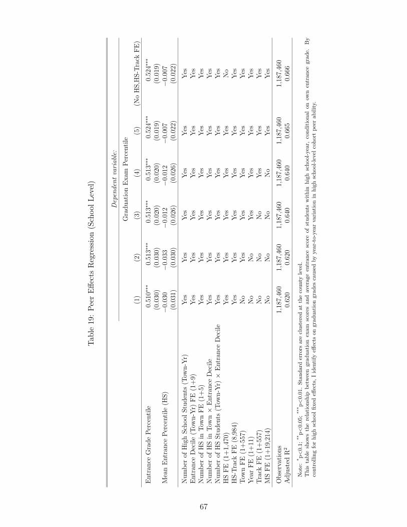
Table19:Pe

erEff

ects

Regression(Schoo

lLevel)

Dep

ende

ntva

riab

le:

Gradu

ationEx

amPe

rcentile

(1)

(2)

(3)

(4)

(5)

(NoHS,HS-Tr

ackFE

)En

tran

ceGrade

Percentile

0.51

0∗∗∗

0.51

3∗∗∗

0.51

3∗∗∗

0.51

3∗∗∗

0.52

4∗∗∗

0.52

4∗∗∗

(0.0

30)

(0.0

30)

(0.0

20)

(0.0

20)

(0.0

19)

(0.0

19)

MeanEn

tran

cePe

rcentile(H

S)−

0.03

0−

0.03

3−

0.01

2−

0.01

2−

0.00

7−

0.00

7(0.0

31)

(0.0

30)

(0.0

26)

(0.0

26)

(0.0

22)

(0.0

22)

Num

berof

HighScho

olStud

ents

(Tow

n-Yr

)Ye

sYe

sYe

sYe

sYe

sYe

sEn

tran

ceDecile

(Tow

n-Yr

)FE

(1+9)

Yes

Yes

Yes

Yes

Yes

Yes

Num

berof

HSin

TownFE

(1+5)

Yes

Yes

Yes

Yes

Yes

Yes

Num

berof

HSin

Town×

Entran

ceDecile

Yes

Yes

Yes

Yes

Yes

Yes

Num

berof

HSStud

ents

(Tow

n-Yr

)×

Entran

ceDecile

Yes

Yes

Yes

Yes

Yes

Yes

HSFE

(1+1,47

0)Ye

sYe

sYe

sYe

sYe

sNo

HS-Tr

ackFE

(8,984

)Ye

sYe

sYe

sYe

sYe

sYe

sTo

wnFE

(1+55

7)No

Yes

Yes

Yes

Yes

Yes

Year

FE(1+11

)No

No

Yes

Yes

Yes

Yes

TrackFE

(1+55

7)No

No

No

Yes

Yes

Yes

MSFE

(1+19

,214

)No

No

No

No

Yes

Yes

Observatio

ns1,18

7,46

01,18

7,46

01,18

7,46

01,18

7,46

01,18

7,46

01,18

7,460

AdjustedR

20.62

00.62

00.64

00.64

00.66

50.66

6

Note:

* p<0.1;

**p<

0.05

;***p<

0.01

.Stan

dard

errors

areclusteredat

thecoun

tylevel.

Thistableshow

stherelatio

nshipbe

tweengrad

uatio

nexam

scores

andaverag

eentran

cescoreof

stud

ents

with

inhigh

scho

ol-year,

cond

ition

alon

ownentran

cegrad

e.By

controlling

forhigh

scho

olfix

edeff

ects,I

identifyeff

ects

ongrad

uatio

ngrad

escaused

byyear-to-year

varia

tionin

high

scho

ol-le

velc

ohortpe

erab

ility.

67

Table 20: Heterogeneity in Peer Effects

Dependent variable:Graduation Exam Percentile

Entrance Grade Percentile 0.522∗∗∗ 0.526∗∗∗

Mean Peer Entrance Percentile −0.067∗∗∗ −0.096∗∗∗

Mean Peer Entrance Percentile × d2 0.012∗∗∗ 0.011∗

Mean Peer Entrance Percentile × d3 0.021∗∗∗ 0.027∗∗∗

Mean Peer Entrance Percentile × d4 0.024∗∗∗ 0.034∗∗∗

Mean Peer Entrance Percentile × d5 0.029∗∗∗ 0.045∗∗∗

Mean Peer Entrance Percentile × d6 0.030∗∗∗ 0.056∗∗∗

Mean Peer Entrance Percentile × d7 0.044∗∗∗ 0.071∗∗∗

Mean Peer Entrance Percentile × d8 0.058∗∗∗ 0.090∗∗∗

Mean Peer Entrance Percentile × d9 0.079∗∗∗ 0.113∗∗∗

Mean Peer Entrance Percentile × d10 0.125∗∗∗ 0.170∗∗∗

Number of High School Students (Town-Yr) Yes YesEntrance Decile (Town-Yr) FE (1+9) Yes YesNumber of HS in Town FE (1+5) Yes YesNumber of HS in Town × Entrance Decile Yes YesNumber of HS Students (Town-Yr) × Entrance Decile Yes YesHS FE (1+1,470) Yes YesHS-Track FE (8,984) Yes YesTown FE (1+557) Yes YesYear FE (1+11) Yes YesTrack FE (1+557) Yes YesMS FE (1+19,214) Yes YesObservations 1,182,897 1,187,460Adjusted R2 0.665 0.666

Note: *p<0.1; **p<0.05; ***p<0.01. Standard errors are clustered at thecounty level.This table shows estimates of hetereogeneity in peer effects, i.e. equation9, where d is the entrance grade decile (at the high school-cohort and highschool-track-cohort levels, respectively).

68

Table 21: Graduation Grades vs Teacher Ability

Dependent variable:Graduation Exam Subject Component (Percentile)

(1) (2) (3) (4) (5)Entrance Grade (Percentile) 0.754∗∗∗ 0.814∗∗∗ 0.801∗∗∗ 0.815∗∗∗ 0.803∗∗∗Teacher 0.079∗∗∗ 0.021∗ 0.026∗∗ 0.024∗ 0.026∗∗d2 × Teacher 0.009 0.011 0.016 0.015d3 × Teacher 0.013 0.016 0.018 0.017d4 × Teacher 0.017 0.020∗ 0.022∗ 0.029∗∗d5 × Teacher 0.023∗ 0.027∗∗ 0.031∗∗ 0.039∗∗∗d6 × Teacher 0.036∗∗ 0.044∗∗∗ 0.048∗∗∗ 0.055∗∗∗d7 × Teacher 0.061∗∗∗ 0.067∗∗∗ 0.073∗∗∗ 0.074∗∗∗d8 × Teacher 0.084∗∗∗ 0.088∗∗∗ 0.099∗∗∗ 0.098∗∗∗d9 × Teacher 0.094∗∗∗ 0.107∗∗∗ 0.117∗∗∗ 0.116∗∗∗d10 × Teacher 0.083∗∗∗ 0.098∗∗∗ 0.108∗∗∗ 0.110∗∗∗

Decile FE (1+9) No Yes Yes Yes YesTown FE (1+587) Yes Yes Yes Yes YesYear FE (1+11) No Yes Yes Yes YesHS FE (1+1,214) No No Yes Yes YesMS FE (1+12,295) No No No Yes YesHS-Track FE (1+7,344) No No No No YesObservations 496,884 496,884 496,884 496,884 496,884Adjusted R2 0.483 0.488 0.500 0.523 0.541

Note: *p<0.1; **p<0.05; ***p<0.01. Standard errors are clustered at the county level.This table presents results of individual student graduation subject scores regressed on entrance scoresand within-school average subject teacher evaluation scores (Teacher). Interactions between entrancescore deciles (d) and teacher ability (Teacher) are also included in order to capture any complemen-tarities between student and teacher ability.

69

Table 22: Decomposition of Sorting Effects (Second Stage): Track Level

Dependent variable:Graduation Exam Component Percentile

(Baseline) (Peers) (Teachers) (Exp) (P+T) (P+T+E)Adm. Score Percentile (Ro) 0.152∗∗∗ 0.151∗∗∗ 0.160∗∗∗ 0.160∗∗∗ 0.160∗∗∗ 0.160∗∗∗

Adm. Score Percentile (Math) 0.061∗∗∗ 0.061∗∗∗ 0.076∗∗∗ 0.078∗∗∗ 0.077∗∗∗ 0.078∗∗∗

Peers (Track) −0.078∗∗∗ −0.049∗∗∗ −0.048∗∗∗

Teachers 0.097∗∗∗ 0.097∗∗∗ 0.098∗∗∗

Expenditures −0.001 −0.002Instrumented Peer Adm. Score (Track) 0.100 0.075 0.021 0.093 −0.001 −0.008Number of High Schools in Town 4 4 4 4 4 4Town-Cohort Adm. Score Decile (d) 10 10 10 10 10 10Number of Students (Town-Cohort) Yes Yes Yes Yes Yes YesNumber of Students (Town-Cohort) × d Yes Yes Yes Yes Yes YesTown Unemployment Level Yes Yes Yes Yes Yes YesCounty HS Dropout Rate Yes Yes Yes Yes Yes YesCounty Average Wage Yes Yes Yes Yes Yes YesTown FE 337 337 337 337 337 337Year FE 5 5 5 5 5 5

Note: *p<0.1; **p<0.05; ***p<0.01. Standard errors are clustered at the county level.This table shows estimation results of Equation 14, using track peers rather than school peers. It shows therelationship between graduation exam subject scores (e.g. math, Romanian) and school quality, proxiedby average admission scores, conditional on own entrance grade. Each column represents a specificationin which I add peer effects, teacher ability and/or school expenditure to the baseline model. Number ofhigh schools are grouped into four bins. Town-cohort admissions core deciles (d) are student entranceexam deciles within their town and cohort; reference level is the bottom entrance grade decile (d1). Peerquality is identified by the differences in within-school average admission scores from year to year. Teacherability is the average placement test percentile of teacher who worked during a student’s four year stay,weighted by the number of weekly hours worked. Since I look at graduation exam components separately,onlyteachers teaching relevant subjects are included on the righ-hand side (e.g. math and physics teachersfor science component grades). Expenditures are measured in hundreds of Euro/student/year. Peeradmission scores are instrumented by an interaction of town-cohort admission deciles and the number ofhigh schools within a town.

70

B Notes on Matching

In this section, I will briefly discuss the matching of graduation records to admission records.

Matching is conducted by student name (as no unique student identifier exists) within high

schools. Thus, students who drop out or change high schools will not be matched. As a note,

high school changes can occur for legitimate reasons (moving, for example) and, anecdotally,

due to corruption.

Table 23 shows summary statistics regarding yearly match rates. Several additional factors,

aside from drop outs and transfers, negatively impact the match rate. Students in many pro-

grams write the high school graduation exam, but do not enter high school via the national

admission exam. For example, students in religious, arts, teaching, sports and architecture,

may be admitted based on other aptitudes, such as playing an instrument, sporting prowess,

knowledge of the Bible, drawing skills, etc. Students in these tracks will not appear in the ad-

mission records. Moreover, some students may repeat a year, while others are former drop-outs

who decide to complete their high school studies.

Likewise, not all high school students admitted to high schools complete the high school

program write the graduation exam. This is the case with students in low-ranked schools

and typically in non-academic or technical programs that aim to prepare students for tertiary

education. Furthermore, students who do not feel confident of passing the exit exam will

sometimes not register for it.

Regarding year to year variation in match rates, generally speaking, the match rate improves

with time. This may be a sign of better data quality or of enforcement of school switching, as

well as changes in drop-out rates.

71

Table 23: Statistics Regarding Yearly Match Rates of Graduating and Entering Students

Min Q1 Median Mean Q3 Max

Graduating Students 56% 59% 64% 66% 71% 75%Entering Students 48% 52% 59% 59% 66% 67%Graduating Students (filtered) 58% 64% 79% 74% 84% 85%Graduating Students (filtered andexcluding technical tracks)

67% 73% 84% 80% 85% 86%

Note: This table contains summary statistics regarding yearly match ratesbetween entering and graduating students. The third line shows match rates forgraduating students, after filtering arts, music, education, architecture, sportsand religious track students, who typically are not admitted through the regularadmission exam, as well as graduating students from previous cohorts. Thefourth line also excludes all technical track students, some of which (dependingon their track), do not gain admission through the entrance exam.

72

C Notes on Sorting

C.1 Student Sorting

Figure 14: Decomposition of Student Entrance Grade Variance by Town Size

0%

25%

50%

75%

100%

1 2 3 4−6 7−15 16+Number of Schools in Town

Per

cent

of T

otal

Var

iatio

n in

Ent

ranc

e G

rade

s

Source ofVariation

StudentLanguage TrackTrackHigh SchoolTown

Note: This figure decomposes the variation in student en-trance scores into: between student (within track) varia-tion, between track variation (within school), between highschool variation (within town) and between town variation,as per Equation 15. The relative contribution of each ofthese sources is then plotted by town size.

I show that student sorting occurs principally at high school level, rather than at the track or

classroom level. I decompose the variation in student entrance scores into different components:

between students who choose the same track and foreign language,42 between different foreign

language choices within the same track, between tracks within the same high school, between

high schools within the same town and between towns, as follows:43N∑i=1

(ei − µe)2 =N∑i=1

(ei − µetrack)2 +N∑i=1

(µelanguage-track − µetrack)2+

N∑i=1

(µetrack − µehs)2 +N∑i=1

(µehs − µetown)2 +N∑i=1

(µetown − µe)2(15)

42When applying to high schools, students can submit their preferences at the “classroom” level. More specif-ically, they can apply to classrooms offering specific tracks (e.g. science, humanities) and specific foreignlanguages to be taught (e.g. English immersion, German). One can identify which track-language program astudent was admitted to in high school using the admission records.

43The proof that this equality holds essentially mirrors the proof that SST = SSR+ SSE for regressions.

73

where e is a student entrance grade and µe is the average entrance grade.44 This will make

it possible to measure at which level sorting is more prevalent. For example, if students were

randomly allocated to schools within towns (and thus there were no school sorting), the fourth

component of equation 15 would be close to zero. On the other hand, if students systematically

sort into high schools by ability, there would be significant variation in mean entrance scores

between high schools and the last component of equation 15 would be large.

In Figure 14, I plot this decomposition of entrance scores for towns of different sizes. The

main takeaway is that the proportion of the total variation in grades explained by between-

school differences is large and increasing in the number of high schools in a town, as illustrated

by the blue area in Figure 14. Indeed, in two high school towns, between high school differences

explain just around 40% of the variation in student entrance grades. In contrast, in large cities,

more than 70% of the variation in student entrance grades can be explained by differences in

average entrance scores between different high schools. In other words, student sorting across

high schools increases markedly in the number of schools in a town.

This is consistent with my initial prediction that a relative consensus about the hierarchy of

high schools exists and that the degree of student sorting is mostly a function of the number of

high school choices available to students.

44Unless otherwise specified, all peer averages in this paper are leave-out averages, i.e. they exclude observationi.

74

Teacher Sorting

I turn towards teacher sorting. In order to better understand to what extent teachers of similar

ability sort into schools, I estimate a model relating a teacher’s individual ability to the average

teacher ability of their coworkers who were hired in the same school:

µthy =β0 + δq + δn + δq×n + δy + δsubject + εi (16)

Here, µthy is the average exam score of teachers in high school h and year y. Fixed effects are

denoted by δ. I use the following fixed effects: exam decile of teacher i within their cohort

and subject, nationally (δd), number of high schools in town l where teacher i works (δn), the

interaction between number of high school and teacher exam score decile (δd×n), year (δy) and

subject (δsubject).

The results of the regression are presented in Table 16 and Figure 15. Teachers who are hired

by schools whose other teachers score higher, on average, on the entrance exam also tend to have

higher scores. Moreover, teachers hired in larger towns tend to score roughly 6 percentile points

higher than those who obtain rural area jobs. Finally, although poorly identified, interaction

terms indicate that teachers hired in high teacher entrance score schools in large towns have

disproportionately high entrance scores compared to those in high entrance score schools in

smaller towns.

On average, teachers hired in top schools in cities score 7 percentiles higher than teachers

hired in top schools in small towns. Teachers hired in bottom quartile schools in cities score 6

percentiles higher than teachers hired in bottom schools in small towns. The average difference

between top and bottom quartile school hires in cities stands at 6 percentiles. In comparison,

this figure is 5 percentiles in one high school towns, highlighting the slightly higher level of

teacher sorting in urban areas. In Appendix C, I show more evidence that teacher sorting

across high schools is increasing in the number of high schools in towns.

I now show that teacher sorting on ability across high schools is increasing in the number

of high schools. In other words, the more high schools there are in a town, the more teachers

sort on ability across these high schools. This is especially true for permanent teachers. Thus,

75

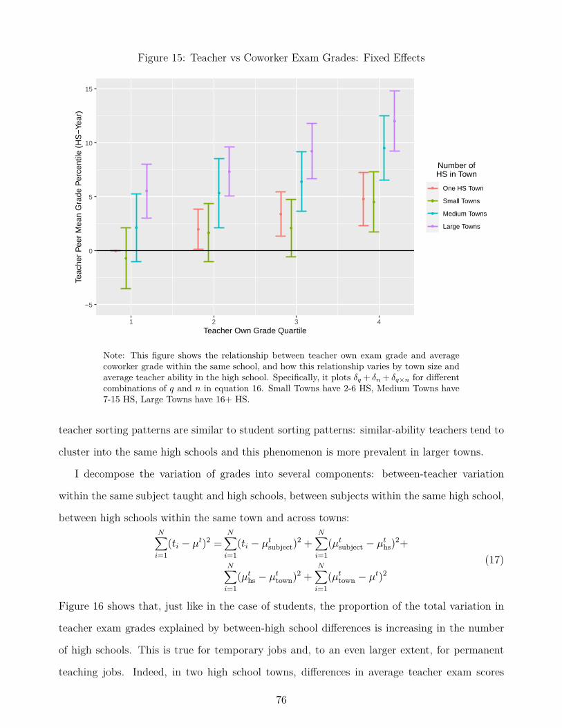
Figure 15: Teacher vs Coworker Exam Grades: Fixed Effects

−5

0

5

10

15

1 2 3 4Teacher Own Grade Quartile

Teac

her

Pee

r M

ean

Gra

de P

erce

ntile

(H

S−

Year

)

Number ofHS in Town

One HS Town

Small Towns

Medium Towns

Large Towns

Note: This figure shows the relationship between teacher own exam grade and averagecoworker grade within the same school, and how this relationship varies by town size andaverage teacher ability in the high school. Specifically, it plots δq + δn + δq×n for differentcombinations of q and n in equation 16. Small Towns have 2-6 HS, Medium Towns have7-15 HS, Large Towns have 16+ HS.

teacher sorting patterns are similar to student sorting patterns: similar-ability teachers tend to

cluster into the same high schools and this phenomenon is more prevalent in larger towns.

I decompose the variation of grades into several components: between-teacher variation

within the same subject taught and high schools, between subjects within the same high school,

between high schools within the same town and across towns:N∑i=1

(ti − µt)2 =N∑i=1

(ti − µtsubject)2 +N∑i=1

(µtsubject − µths)2+

N∑i=1

(µths − µttown)2 +N∑i=1

(µttown − µt)2(17)

Figure 16 shows that, just like in the case of students, the proportion of the total variation in

teacher exam grades explained by between-high school differences is increasing in the number

of high schools. This is true for temporary jobs and, to an even larger extent, for permanent

teaching jobs. Indeed, in two high school towns, differences in average teacher exam scores

76

Figure 16: Decomposition of Teacher Exam Grade Variance by Town Size

Permanent Jobs Temporary Jobs

1 2 3 4−6 7−15 16+ 1 2 3 4−6 7−15 16+

0%

25%

50%

75%

100%

Number of Schools in Town

Per

cent

of T

otal

Var

iatio

n in

Tea

cher

Eva

luat

ions

Source ofVariation

TeacherSubjectHigh SchoolTown

Note: This figure decomposes the variation in teacherexam scores into: between teacher variation (within sub-ject taught and in the same high school), between subjectvariation (within high school), between high school varia-tion (within town) and between town variation. The rel-ative contribution of each of these sources is then plottedby town size.

between high schools account for less than 10% (15%) of the total variation in teacher scores

for permanent (temporary) jobs. In contrast, for cities, between school differences account for

more than 50% (25%) of the total variation in teacher exam scores.

77

D Identification Concerns and Robustness Checks

The Heckman selection procedure implemented uses the proportion of a student’s middle school

classmates who drop out of high school, interacted with a student’s grade in a probit model

to predict a student’s probability of dropping out, as per Wooldridge (2002). The idea is that

a student’s middle school peers may exert indirect influence on a student’s decision to drop

out, without having an influence on student performance at school, conditional on the student’s

entrance score and middle school attended. Then, the estimates of this model are used to

compute an inverse Mills ratio (λ) used as a regressor in the first and second stages of the

IV estimation. First, the sample selection equation, which includes all exogenous variables, is

estimated via probit:

dropi =1[ψ0 + ψmms dropmy + ψmdms dropmy × δd + ψeei + δn + δd + δl + δm+

δp + δy + δs + δs×d + εi]

where dropi is a an indicator of whether student i dropped out from high school (i.e. they

have a high school entrance grade, but no corresponding graduation grade), ms dropmy is the

proportion of high school drop outs in cohort y of middle school m. The inverse Mills ratio is

computed as:

λi = φ(d̂ropi)Φ(d̂ropi)

where φ is the standard normal probability density function and Φ is the standard normal

cumulative probability function. The first and second stages of the IV estimation will then

include this new variable. The second stage is:

gi = β0 + βeei + βµµe-ihy + δn + δd + δl + δm + δp + δy + δs + δs×d + βλλi + εi

and the first stage is:

µehy = γ0 + γeei + ηn + ηd + ηd×n + ηm + ηl + ηp + ηy + ηs + ηs×d + ηλλi + ξi

The results of the selection equation are presented in Table 24. Conditional on their entrance

scores and ranking within town-cohort, students who attended a high drop-out rate middle

school are more likely to drop out of high school, and this effect is more pronounced for students

78

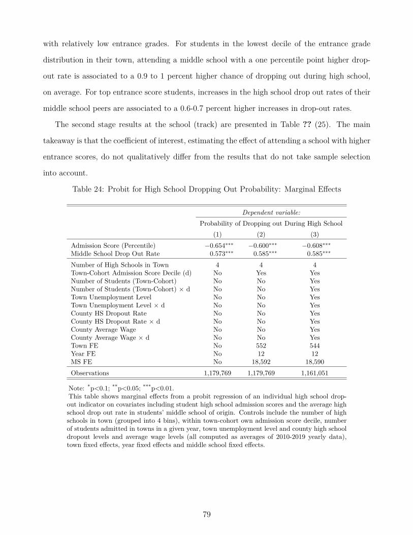
with relatively low entrance grades. For students in the lowest decile of the entrance grade

distribution in their town, attending a middle school with a one percentile point higher drop-

out rate is associated to a 0.9 to 1 percent higher chance of dropping out during high school,

on average. For top entrance score students, increases in the high school drop out rates of their

middle school peers are associated to a 0.6-0.7 percent higher increases in drop-out rates.

The second stage results at the school (track) are presented in Table ?? (25). The main

takeaway is that the coefficient of interest, estimating the effect of attending a school with higher

entrance scores, do not qualitatively differ from the results that do not take sample selection

into account.

Table 24: Probit for High School Dropping Out Probability: Marginal Effects

Dependent variable:Probability of Dropping out During High School

(1) (2) (3)Admission Score (Percentile) −0.654∗∗∗ −0.600∗∗∗ −0.608∗∗∗Middle School Drop Out Rate 0.573∗∗∗ 0.585∗∗∗ 0.585∗∗∗

Number of High Schools in Town 4 4 4Town-Cohort Admission Score Decile (d) No Yes YesNumber of Students (Town-Cohort) No No YesNumber of Students (Town-Cohort) × d No No YesTown Unemployment Level No No YesTown Unemployment Level × d No No YesCounty HS Dropout Rate No No YesCounty HS Dropout Rate × d No No YesCounty Average Wage No No YesCounty Average Wage × d No No YesTown FE No 552 544Year FE No 12 12MS FE No 18,592 18,590Observations 1,179,769 1,179,769 1,161,051

Note: *p<0.1; **p<0.05; ***p<0.01.This table shows marginal effects from a probit regression of an individual high school drop-out indicator on covariates including student high school admission scores and the average highschool drop out rate in students’ middle school of origin. Controls include the number of highschools in town (grouped into 4 bins), within town-cohort own admission score decile, numberof students admitted in towns in a given year, town unemployment level and county high schooldropout levels and average wage levels (all computed as averages of 2010-2019 yearly data),town fixed effects, year fixed effects and middle school fixed effects.

79

Table 25: IV Second Stage (Track Level) with Heckman Correction

Dependent variable:Graduation Exam Score (Percentile)(1) (2) (3)

Admission Score (Percentile) 0.367∗∗∗ 0.322∗∗∗ 0.356∗∗∗Inverse Mills Ratio 0.086∗∗∗ 0.005 0.005Instrumented Peer Admission Score (Percentile) 0.341∗∗∗ 0.246∗∗∗ 0.353∗∗∗

Number of High Schools in Town 4 4 4Town-Cohort Admission Score Decile (d) No Yes YesNumber of Students (Town-Cohort) No No YesNumber of Students (Town-Cohort) × d No No YesTown Unemployment Level No No YesTown Unemployment Level × d No No YesCounty HS Dropout Rate No No YesCounty HS Dropout Rate × d No No YesCounty Average Wage No No YesCounty Average Wage × d No No YesTown FE No 552 544Year FE No 12 12MS FE No 18,592 18,590Observations 1,179,769 1,179,769 1,161,051

Note: *p<0.1; **p<0.05; ***p<0.01.

This table shows second stage results form the equation 3. Student graduation exams scores(in percentiles at the cohort-country level) are regressed on similar admission scores and peeradmission scores. Peer admission scores (at the school level) are instrumented using an interac-tion between student’s own admission score decile and the number of high schools int he townin which they attend high school. Controls include the number of high schools in town (groupedinto 4 bins), within town-cohort own admission score decile, number of students admitted intowns in a given year, town unemployment level and county high school dropout levels andaverage wage levels (all computed as averages of 2010-2019 yearly data), town fixed effects, yearfixed effects and middle school fixed effects.

80

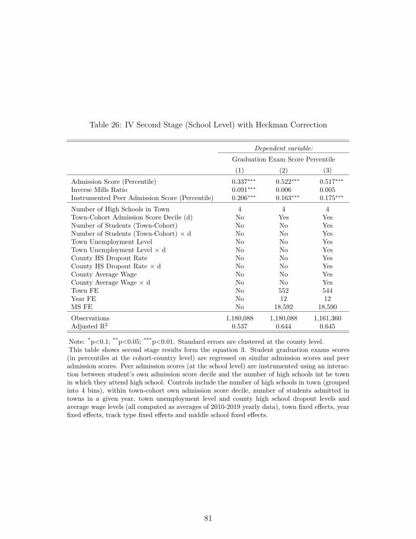
Table 26: IV Second Stage (School Level) with Heckman Correction

Dependent variable:Graduation Exam Score Percentile(1) (2) (3)

Admission Score (Percentile) 0.337∗∗∗ 0.522∗∗∗ 0.517∗∗∗Inverse Mills Ratio 0.091∗∗∗ 0.006 0.005Instrumented Peer Admission Score (Percentile) 0.206∗∗∗ 0.163∗∗∗ 0.175∗∗∗

Number of High Schools in Town 4 4 4Town-Cohort Admission Score Decile (d) No Yes YesNumber of Students (Town-Cohort) No No YesNumber of Students (Town-Cohort) × d No No YesTown Unemployment Level No No YesTown Unemployment Level × d No No YesCounty HS Dropout Rate No No YesCounty HS Dropout Rate × d No No YesCounty Average Wage No No YesCounty Average Wage × d No No YesTown FE No 552 544Year FE No 12 12MS FE No 18,592 18,590Observations 1,180,088 1,180,088 1,161,360Adjusted R2 0.537 0.644 0.645

Note: *p<0.1; **p<0.05; ***p<0.01. Standard errors are clustered at the county level.This table shows second stage results form the equation 3. Student graduation exams scores(in percentiles at the cohort-country level) are regressed on similar admission scores and peeradmission scores. Peer admission scores (at the school level) are instrumented using an interac-tion between student’s own admission score decile and the number of high schools int he townin which they attend high school. Controls include the number of high schools in town (groupedinto 4 bins), within town-cohort own admission score decile, number of students admitted intowns in a given year, town unemployment level and county high school dropout levels andaverage wage levels (all computed as averages of 2010-2019 yearly data), town fixed effects, yearfixed effects, track type fixed effects and middle school fixed effects.

81