scholarships at risk: the mathematics of merit

UC Irvine Law ReviewVolume 7Issue 1 Higher Education Access Article 4

1-2017

Scholarships at Risk: The Mathematics of MeritStipulations in Financial Aid AwardsJames Ming [email protected]

Follow this and additional works at: https://scholarship.law.uci.edu/ucilr

This Article is brought to you for free and open access by UCI Law Scholarly Commons. It has been accepted for inclusion in UC Irvine Law Review byan authorized editor of UCI Law Scholarly Commons.

Recommended CitationJames M. Chen, Scholarships at Risk: The Mathematics of Merit Stipulations in Financial Aid Awards, 7 U.C. Irvine L. Rev. 43 (2017).Available at: https://scholarship.law.uci.edu/ucilr/vol7/iss1/4

https://scholarship.law.uci.edu/ucilr?utm_source=scholarship.law.uci.edu%2Fucilr%2Fvol7%2Fiss1%2F4&utm_medium=PDF&utm_campaign=PDFCoverPages

https://scholarship.law.uci.edu/ucilr/vol7?utm_source=scholarship.law.uci.edu%2Fucilr%2Fvol7%2Fiss1%2F4&utm_medium=PDF&utm_campaign=PDFCoverPages

https://scholarship.law.uci.edu/ucilr/vol7/iss1?utm_source=scholarship.law.uci.edu%2Fucilr%2Fvol7%2Fiss1%2F4&utm_medium=PDF&utm_campaign=PDFCoverPages

https://scholarship.law.uci.edu/ucilr/vol7/iss1/4?utm_source=scholarship.law.uci.edu%2Fucilr%2Fvol7%2Fiss1%2F4&utm_medium=PDF&utm_campaign=PDFCoverPages

https://scholarship.law.uci.edu/ucilr?utm_source=scholarship.law.uci.edu%2Fucilr%2Fvol7%2Fiss1%2F4&utm_medium=PDF&utm_campaign=PDFCoverPages

https://scholarship.law.uci.edu/ucilr/vol7/iss1/4?utm_source=scholarship.law.uci.edu%2Fucilr%2Fvol7%2Fiss1%2F4&utm_medium=PDF&utm_campaign=PDFCoverPages

Final to Printer_Chen (Do Not Delete) 9/19/2017 8:30 AM

43

Scholarships at Risk: The Mathematics of Merit Stipulations in Financial Aid Awards

James Ming Chen*

Introduction: Forewarned Is Forearmed ...................................................................... 43 I. The Expected Value of Financial Aid Subject to a Merit Stipulation................... 45 II. Evaluating Merit Stipulations According to a Law School’s Break-Even

Point ....................................................................................................................... 48 III. A Statistical Moment or Two: From Standard Scores to Value-at-Risk

Analysis .................................................................................................................. 51 A. Standard Scores and Grading on a Curve ............................................... 52 B. Estimating the Probability of Failure to Satisfy a Merit

Stipulation .................................................................................................... 55 IV. Scholarships at Risk: Extrapolating Mean Grades and Standard

Deviation Through an Application of Value-at-Risk Analysis ..................... 63 Conclusion .......................................................................................................................... 71

INTRODUCTION: FOREWARNED IS FOREARMED

American law schools often condition financial aid grants on the maintenance of a certain grade point average (GPA).1 “Merit stipulations,” as these conditions are known, require that students meet or exceed minimum academic standards, typically at the end of their first year in law school. Students must meet these stipulations in order to keep all or part of their financial aid for the remaining two years of law study.2 Many law schools charge $40,000 or more in annual tuition.3 The grants they award routinely carry a face value of $15,000, theoretically

* Justin Smith Morrill Chair in Law, Michigan State University; Of Counsel, Technology Law Group of Washington, D.C. Ann Levine, Jerome M. Organ, and Brian Tamanaha provided helpful comments. Special thanks to Heather Elaine Worland Chen.

1. See Jerome M. Organ, How Scholarship Programs Impact Students and the Culture of Law School, 61 J. LEGAL EDUC. 173, 173–74 (2011).

2. David Segal, Behind the Curve: How Law Students Lose the Grant Game, and How Their Schools Win, N.Y. TIMES, May 1, 2011, at BU6.

3. Debra Cassens Weiss, Tuition and Fees at Private Law Schools Break $40K Mark, on Average, ABA JOURNAL (Aug. 20, 2012, 10:30 AM), http://www.abajournal.com/news/article/average_tuition_at_private_law_schools_breaks_40k_mark [https://perma.cc/RGF9-8VWW].


44 UC IRVINE LAW REVIEW [Vol. 7:43

renewable for all three years of full-time law study.4 But the very existence of a merit stipulation discounts the value of a grant. That discount can, and should, be calculated according to the probability that a student may fail to fulfill the merit stipulation attached to her or his financial aid grant.

Students should take merit stipulations into account when they decide whether to accept an offer of admission paired with a conditional grant of financial aid. By all accounts, they do not. Law schools should transparently disclose the likely effect of merit stipulations on their financial aid awards and, by extension, the likely impact of a lost award on the affected student’s future financial well-being. By all accounts, law schools do no such thing. Absent external coercion, they are unlikely to change their current practices. Although the Law School Admissions Council (LSAC) and the American Bar Association (ABA) do urge law schools to provide full consumer information to prospective students, neither the LSAC nor the ABA requires full, transparent disclosure of the probability that a merit stipulation will result in the partial or full loss of financial aid.5 Instead, many schools merely state the terms of their merit stipulation. In order to retain their grants in full, students must meet some GPA target, such as 2.95 or 3.2.6

Prospective students need and deserve fuller information regarding financial aid. Financial and moral responsibility demands no less of law schools.7 Although I have framed the problem as one stemming from the exigencies of legal education, this problem arises in any educational setting where financial aid is conditioned upon the maintenance of a particular GPA. Furthermore, even though I have made no real effort to assess the impact of merit stipulations or other financial aid practices on access, opportunity, and diversity in higher education, there is universal awareness that indebtedness undermines every one of these socially progressive objectives.8

In the absence of industry-wide standards counseling full disclosure of financial aid practices, this Article will take a first step toward equipping prospective students to assess their own economic prospects. This Article will frame the problem of merit stipulations in law school financial aid as one of applied mathematics. Schools often do offer enough information for prospective students

4. See Which Private Law Schools Award the Most Financial Aid?, U.S. NEWS & WORLD

REPORT, http://grad-schools.usnews.rankingsandreviews.com/best-graduate-schools/top-law-schools/finaid-private-rankings?int=98ee08 [https://perma.cc/QFV2-87KS] (last visited July 24, 2016); Which Public Law Schools Award the Most Financial Aid?, U.S. NEWS & WORLD REPORT, http://grad-schools.usnews.rankingsandreviews.com/best-graduate-schools/top-law-schools/finaid-public-rankings [https://perma.cc/BQC5-MGAW] (last visited July 24, 2016).

5. Organ, supra note 1, at 195–96, 195 n.45. 6. See Segal, supra note 2, at BU6. 7. See Jim Chen, A Degree of Practical Wisdom: The Ratio of Educational Debt to Income as a

Basic Measurement of Law School Graduates’ Economic Viability, 38 WM. MITCHELL L. REV. 1185, 1185–87 (2012).

8. See, e.g., Deborah J. Merritt, Race, Debt, and Opportunity, LAW SCHOOL CAFE (Mar. 10, 2016), http://www.lawschoolcafe.org/2016/03/10/race-debt-and-opportunity [https://perma.cc/HEL2-FDJM].


2017] THE MATHEMATICS OF MERIT STIPULATIONS 45

to evaluate, with some degree of accuracy, the actual cost of attendance. I hope that this Article completes the informational package and enables prospective students to make fully informed decisions about their education and their professional future.

Part I of this Article outlines a simple methodology for calculating the expected value of a financial aid award subject to a merit stipulation. Part II evaluates one extraordinary circumstance in which a law school (Chicago-Kent) has implicitly revealed its break-even point—the amount of aid that the school would award if it could not impose any merit stipulations on a scholarship recipient. These preliminary steps serve as a prelude to the heart of this Article.

Part III performs a comprehensive analysis of law school grades and merit stipulations as artifacts of the standard normal distribution—also known as the Gaussian distribution in honor of Carl Friedrich Gauss. Part III performs three distinct tasks. First, it defines standard scores. Second, it explains how law school grading is based on the relationship between the standard score of each student’s raw score and the mean and standard deviation of the distribution as a whole. Finally, Part III describes the risk of failure to satisfy a merit stipulation in terms of the normal distribution’s cumulative distribution function.

For those instances in which the risk of failure to satisfy a particular school’s merit stipulation is known (if only through negative reporting in the press), Part IV of this Article demonstrates how to use the quantile function, or inverse cumulative distribution function, to estimate the mean and standard deviation of a school’s grade distribution. This final exercise represents an academic application of value-at-risk analysis, a leading tool for assessing market risk in American and global capital markets.

I. THE EXPECTED VALUE OF FINANCIAL AID SUBJECT TO A MERIT STIPULATION

In his 2011 series of articles on legal education, David Segal of the New York Times shed unflattering light on the financial aid practices of American law schools.9 He took special aim at merit stipulations, or “stips,” as a tool that enhances law schools’ U.S. News and World Report rankings at the expense of their students.10 Merit scholarships, on any terms, have become much more commonplace in American legal education:

Nobody knows exactly how many law school students nationwide lose scholarships each year—no oversight body tallies that figure—but what’s clear is that American law schools have quietly gone on a giveaway binge in the last decade. In 2009, the most recent year for which the American Bar Association has data, 38,000 of 145,000 law school students—more than one in four—were on merit scholarships. The total tab for all schools in all three years: more than $500 million.11

9. See Segal, supra note 2. 10. Id. at BU1, BU6. 11. Id. at BU6.



The typical merit stipulation merely states the minimum GPA that a student must maintain in order to continue receiving financial aid, or at least the full amount of the grant awarded at the time of admission.12 According to Mr. Segal, “[t]he University of Florida’s law school requires students to maintain a 3.2 GPA to keep their scholarships; at the Benjamin N. Cardozo School of Law in Manhattan, it’s a 2.95.”13 Some merit stipulations target first-year grades. This practice appears to be prevalent, and perhaps even dominant, throughout American legal education.

In his study of financial aid practices at American law schools, Professor Jerome Organ assumes that schools enforce merit stipulations at the end of the first year of study, but not between the second and third years.14 Even if schools do enforce merit stipulations throughout all three years, upper-level grades correlate so strongly with first-year grades that passing through the 1L bottleneck may provide a good starting point for quantifying the financial impact of merit stipulations.

Much of Mr. Segal’s article focused on the Golden Gate University School of Law in San Francisco.15 According to Mr. Segal, “57 percent of first-year students” who entered Golden Gate “—more than 150 in a class of 268—ha[d] merit scholarships.”16 Mr. Segal also reported, however, that “in recent years, only the top third of students at Golden Gate wound up with a 3.0 or better” after one year of law study.17 According to Golden Gate’s own description of its entering class, its full-time J.D. program consisted of 229 students.18 Adding thirty-three students in the honors lawyering program brings the total of full-time matriculants to 262, much closer to the number reported by the New York Times.19 Although the information may not be complete enough to warrant this inference, it appears that 153 Golden Gate students received some sort of award (57% of the 269 counted by the Times).20

These facts provide the basis for our first and simplest exercise in evaluating the probable economic impact of a merit stipulation on financial aid. In fairness to Golden Gate, I will treat that school’s 269 full-time students as the entering cohort at a wholly fictional school, the Silver Path College of Law. I further stipulate that Silver Path charges $38,375 per year as “sticker price” tuition, before discounts are applied in the form of financial aid. Fifty-seven percent of this entering class (153 students out of 269) receive aid. The average award per student receiving aid is $14,683. Silver Path does enforce a merit stipulation: students receiving aid must finish the first year of law studies with a GPA no less than 3.0. Failure to attain at least a 3.0 GPA results in the complete loss of financial aid. Only the top third of

12. Id. 13. Id. 14. See Organ, supra note 1, at 179, 194. 15. Segal, supra note 2. 16. Id. at BU6. 17. Id. 18. Admissions, GGU LAW (Apr. 21, 2012), http://law.ggu.edu/admissions [https://

web.archive.org/web/20120421023553/http://law.ggu.edu/admissions]. 19. Id. 20. Id.



Silver Path’s first-year class satisfies this 3.0 threshold. These are ultimately stylized figures, not a detailed analysis of the financial aid situation at Golden Gate or any other actual school.

Our initial question is a simple one: What is the expected value of a $14,683 financial aid award from the Silver Path College of Law? I will adopt certain simplifying assumptions. Even though there is strong reason to believe that Silver Path directs its financial aid in a strategic effort to enhance its standing within the U.S. News and World Report ’s annual law school rankings,21 and even though the leading indicators of preparedness for law study are highly correlated with actual grades in law school, I will assume that financial aid is randomly distributed within the entering class. I will further assume that a scholarship recipient and a student paying full fare face equal odds of any given academic outcome after matriculation. Finally, I will dispense with discount rates, the cost of debt service, and every other adjustment rooted in the assumption that money has nonzero time value.

From the perspective of a rational student weighing Silver Path’s scholarship offer, the school’s award of $14,683 for each year of law school, subject to a one-time merit stipulation enforced at the end of the first year, has the following expected value:

Year 1: $14,683 × 1.00 probability ≈ $14,683 expected value Year 2: $14,683 × 0.33 probability ≈ $4,894 expected value Year 3: $14,683 × 0.33 probability ≈ $4,894 expected value

Over three years, this award has a total expected value of approximately $24,472.22 The annual value of that award is the total divided by three, or $8,157.

More generally, the expected value of a financial aid award subject to a merit stipulation enforced at the end of the first year of law study is expressed by the following equation:

where E represents the expected annualized value of the award, F represents the face value of the award per year, and p represents the probability of renewal upon satisfaction of the merit stipulation. Substituting one-third for p dictates that F, the $14,683 face value of the award, be evaluated at five-ninths of its value, or

21. See Organ, supra note 1, at 176 (internal citation omitted) (adopting the assumption that no law school “is interested in distributing scholarship money evenly among all students” and that law schools “distribute scholarship assistance across their pools of applicants in an effort to get the pool of students with the highest median LSAT and GPA, because these are two of the key reference points in the U.S. News & World Report ’s rankings system”).

22. I have rounded all numbers to the nearest dollar.

E 1 2p

3 F



5

9

approximately 55.6%. , after all, equals .

This is a straightforward calculation of expected value. We nevertheless have reason to believe that law students do not approach the problem as one of mathematics or probability. In his interview by David Segal of the New York Times, Dean Harold J. Krent of the Chicago-Kent College of Law lamented, “The real issue is that students don’t think about this decision in the sophisticated way that you’d like them to. . . . A lot of students think, ‘Well, worst comes to worst, I’ll borrow the money,’ without realizing how painful it is to pay that money back over time.”23 If Dean Krent’s assessment bears any resemblance to behavioral reality, then the factor that wields outsized influence over student decisions is F, the face value of a law school’s financial aid offer. The trouble is that the variable that truly dictates students’ financial future is E, the expected value of the award, discounted by the probability of loss traceable to a failure to uphold the award’s merit stipulation.

II. EVALUATING MERIT STIPULATIONS ACCORDING TO A LAW SCHOOL’S

BREAK-EVEN POINT

The previous section’s discussion of financial aid at the partially fictionalized Silver Path College of Law rested on the premise that a law school would reveal the exact rate at which it expects students to fall short of the merit stipulation in their financial aid awards. Such straightforward disclosure should be standard practice in American legal education.24 But it is not. Law schools nevertheless do disclose information that enables students to estimate the rate at which grant recipients fail to meet a merit stipulation. The Chicago-Kent College of Law provides the factual backdrop for an exercise in estimating the probability of failure based on a law school’s de facto disclosure of the point at which it would break even on its financial aid awards, relative to a known financial baseline.

Once again, David Segal’s quick survey of financial aid practices among American law schools sets the stage:

The Chicago-Kent College of Law has a number of grant offerings, one of which sounds like the refueling options for a rental car: students can get a $9,000 annual scholarship guaranteed for all three years, no matter what their G.P.A., or $15,000 a year on the condition that they earn a 3.25 or above. If they get between a 3.0 and 3.25, they keep half the scholarship. Below a 3.0, it’s gone.25

23. Segal, supra note 2, at BU7. 24. See Organ, supra note 1, at 194. 25. Segal, supra note 2, at BU6.

3

321



Although Chicago-Kent did not disclose the probability that a student would satisfy this set of merit stipulations, that school did provide ample information by which we may make a well-informed set of projections.

Chicago-Kent’s willingness to award a guaranteed scholarship worth $9,000 a year sets a financial baseline by which we may evaluate the superficially generous but fundamentally riskier option of $15,000 subject to a matching pair of merit stipulations. We again assume that the GPA hurdle applies exactly once, at the end of the first year. We again dispense with discount rates and other complexities arising from the time value of money. On these simplifying assumptions, Chicago-Kent’s guaranteed financial aid option is obviously worth 3 × $9,000, or $27,000. If we presume that Chicago-Kent is indifferent as between offering the guaranteed award and offering the conditional award—as a rational institutional actor assuredly would be—then the expected value of the conditional award should be the same as the guaranteed award.

Let p3.25 represent the probability that a scholarship recipient at Chicago-Kent fully satisfies the merit stipulation by achieving a first-year GPA of 3.25 or higher. Let p3.00 represent the probability that a scholarship recipient partially satisfies the merit stipulation by achieving a first-year GPA greater or equal to 3.00, but less than 3.25. Failure to meet even the lower 3.00 GPA threshold results in complete loss of the scholarship. In the interest of completeness, we can assign this probability to the variable p<3.00. Because these three probabilities exhaust the universe of possible outcomes, . The expected value of the conditional scholarship over three years is represented by the following equation:

With simplification:

We must solve for two variables with a single equation. That is not algebraically possible. But we can make an informed guess. Holding p3.00 at 0 implies a maximum value of 0.4 for p3.25 ($4,000/$10,000 = 0.4). Holding p3.25 at 0 implies a maximum value of 0.8 for p3.00 ($4,000/$5,000 = 0.8). Neither extreme is realistic. On the other hand, the arbitrary expedient of splitting the difference between extremes yields a solution that is at once simple, workable, and even elegant. At the midpoint of these ranges—p3.25 = 0.2 and p3.00 = 0.4—the probabilistically adjusted expected value of each outcome makes an equal contribution toward the three-year expected value of 3E. If $15,000 of the expected value of 3E = $27,000 is achieved in the first year, then setting p3.25 = 0.2 and p3.00 = 0.4 adds $6,000 each to these expected outcomes: A 0.2 probability of keeping $30,000 over the final two years of law school produces $6,000 of expected value. A 0.4 probability of keeping $15,000 over the final two years of law school also produces $6,000 of expected value. $15,000 + (2 × $6,000) = $27,000.

p3.25 p3.00 p3.00 1

3E $15,000 p3.25 2 $15,000 p3.00 2 $7,500 p3.00 2 $0 $27,000

p3.25 $10,000 p3.00 $5,000 $4,000



The relationship between p3.25 and p3.00 is straightforward. It allows us to build a little room for guesswork in what is an inescapably imprecise mathematical exercise. (It bears repeating that you cannot solve for two variables with a single equation.) Designating every unit of change in p3.25 as p3.25 allows us to state, formally, that p3.00 moves in the opposite direction by two units for every unit of p3.25:

In other words, for every student who achieves a GPA exceeding 3.25, we should expect two other students to fall short of a 3.00 GPA. Some actual numbers may enable us to see this relationship more clearly. If we fix p3.25 at 0.16, or 0.2 minus 0.04, then the value of p3.00 will be 0.48, or 0.4 plus 0.08. If we fix p3.25 at 0.24, or 0.2 plus 0.04, then p3.00 will equal 0.32, or 0.4 minus 0.08. For values of p3.25 = 0.2 ± 0.04, p3.00 = 0.4 ± 0.08. Within these values, the ratio p3.00/p3.25 ranges from 1.33 to 3.00:

Unlike many (if not most) other law schools that place academic conditions on their financial aid offers, Chicago-Kent offers its students a choice.26 The truly curious aspect of Chicago-Kent’s arrangement is the frequency with which students choose each option, either the safer but smaller amount of $9,000, guaranteed over three years, or the flashier but shakier amount of $15,000, subject to a merit stipulation. Given what must be Chicago-Kent’s obvious message—that a guaranteed $9,000 scholarship offer is financially equivalent to a “teaser” scholarship of $15,000 subject to the school’s two-tiered merit stipulation—one would expect students to choose each of the two options with roughly equal frequency. If one accounts for risk aversion, especially in a population as reputedly risk-averse as law students, one would expect Chicago-Kent students to flock affirmatively to the safer, guaranteed $9,000 option. One would be wrong on both counts. According to Dean Krent and his colleagues, “[n]inety percent” of Chicago-Kent students offered this choice between scholarships “opt for the larger and riskier sum.”27 Not surprisingly, a “‘significant’ number later lose their scholarships.”28

Garrison Keillor purportedly set his imaginary Lake Wobegon among roughly ten thousand other bodies of fresh water in Minnesota.29 The host of Prairie Home

26. Id. 27. Id. 28. Id. 29. See GARRISON KEILLOR, LAKE WOBEGON DAYS (1990); see also Minnesota, WIKIPEDIA,

http://en.wikipedia.org/wiki/Minnesota [https://perma.cc/33U4-QURL] (last modified Sept. 11, 2016).

1.33 p3.00

p3.25

3.00



Companion is nothing if not a master of misdirection. Behavioral evidence from Chicago-Kent places Lake Wobegon closer to Cook County’s legendary Gold Coast.30 Like residents of Lake Wobegon, most human beings believe—in defiance of the laws of probability—they are above average in ability.31 Notwithstanding their school’s effort to inoculate them against the emotional and financial trauma of a de facto $15,000 tuition increase after one year of legal education, many Chicago-Kent students quite evidently place themselves at some considerable positive distance from that school’s class mean.32

III. A STATISTICAL MOMENT OR TWO: FROM STANDARD SCORES TO VALUE-AT-RISK ANALYSIS

Our incomplete, but reasonably well-informed, evaluation of Chicago-Kent’s merit stipulation leads to a final exercise. Once we know the probability that a scholarship recipient will satisfy the merit stipulation on her or his award, applied mathematics enables us to estimate the mean grade and the standard deviation of GPAs within a particular law school. Indeed, both the real financial aid policies of Chicago-Kent and the stylized policies of Silver Path (the thinly disguised surrogate for Golden Gate) provide fodder for a further mathematical adventure.

We are told, flat-out, that merit stipulations eliminate all but a third of financial aid awards at Silver Path at the 3.0 GPA threshold. We surmise that Chicago-Kent predicts that two-tenths of its students will meet or exceed the 3.25 GPA benchmark and another four-tenths will land between 3.00 and 3.25. Even if we allow some room for error in our evaluation of the 3.25 GPA benchmark, as in p3.25 ≈ 0.2 ± 0.04, the relationship between that benchmark and the 3.00–3.25 GPA benchmark enables us to estimate the probability associated with this lower GPA range within a comparably narrow range: p3.00 ≈ 0.4 ± 0.08. This information enables us to make educated guesses about grades at both schools. We can predict the overall GPA and the approximate distribution of GPAs among students at those schools. Indeed, since many American law schools publish their grade distributions,33 which are then aggregated at sources such as the NALP Directory of Law Schools34 and even Wikipedia,35 the analysis I am about to outline should enable any prospective student to make an educated (and in some cases, depressingly

30. See generally Segal, supra note 2. 31. See generally Justin Kruger, Lake Wobegon Be Gone! The “Below-Average Effect” and the

Egocentric Nature of Comparative Ability Judgments, 77 J. PERSONALITY & SOC. PSYCHOL. 221, 221 (1999).

32. Segal, supra note 2, at BU6–BU7. 33. See, e.g., Grades & Quartiles, U. OF MINN. L. SCH., http://www.law.umn.edu/careers/

grades.html [https://perma.cc/FM6Y-PAJM] (last visited Sept. 12, 2016) (reporting that the University of Minnesota Law School requires first-year grades to fall between a 3.0000 and 3.3333 GPA and recommends the same grade range for upper-level courses).

34. See NALP Directory of Law Schools, NALP, http://www.nalplawschoolsonline.org [https:// perma.cc/5XBZ-3B25] (last visited Sept. 12, 2016).

35. List of Law School GPA Curves, WIKIPEDIA, http://en.wikipedia.org/wiki/List_of_ law_school_GPA_curves [https://perma.cc/46XX-MTHD] (last modified Aug. 12, 2016).



accurate) guess about the likelihood that she or he will satisfy a merit stipulation on an offer of financial aid.

This exercise is made possible by a statistical artifact of academic grading. Although the world of risk assessment and management is slowly, grudgingly coming to grips with the reality that many probabilities refuse to follow the symmetrical “bell curve” of the Gaussian distribution,36 there is a reason that the Gaussian distribution is considered the “normal” distribution. Many physical and social phenomena follow the normal, Gaussian distribution.37 Academic grading is one of those phenomena. Sometimes, we really can allow ourselves to be seduced by the mathematical elegance of “beautifully Platonic models on a Gaussian base.”38 Deciphering law school grade distributions is one of those times. Let us now turn to the task at hand.

A. Standard Scores and Grading on a Curve

We should begin by defining standard scores, also known as z-scores.39 In statistical terms, a grade is simply a scaled score, or a digestible expression of a raw score that has been converted to a standard score according to the multiple of standard deviations by which the raw score departs from the arithmetic mean of the whole population of grades. Let x represent the raw score; let z represent the scaled score. Conventional statistical notation uses μ (mu) to designate the mean of the population and σ (sigma) to designate that population’s standard deviation.40 The standard score z of a raw score x is:

With varying degrees of awareness, nearly all academics (and not just in law) engage in some variation on the theme of standard scoring when they assign grades.41 In practice, most values of z will be greater than –2 and less than 2. Absolute values of z exceeding 2 correspond to true outliers. Those students are either ironclad locks for the book award, or good candidates for receiving an F. In

36. See, e.g., Daniel A. Farber, Probabilities Behaving Badly: Complexity Theory and Environmental Uncertainty, 37 U.C. DAVIS L. REV. 145, 146–47 (2003).

37. See, e.g., GEORGE CASELLA & ROGER L. BERGER, STATISTICAL INFERENCE 102 (Duxbury Press, 2d ed. 2002) (1990).

38. NASSIM NICHOLAS TALEB, THE BLACK SWAN: THE IMPACT OF THE HIGHLY

IMPROBABLE 277 (2007). 39. See generally Standard Score, WIKIPEDIA, http://en.wikipedia.org/wiki/Standard_score

[https://perma.cc/WLD4-JUDT] (last modified Sept. 9, 2016). 40. See Standard Deviation, WIKIPEDIA, https://en.wikipedia.org/wiki/Standard_deviation

[https://perma.cc/6SEU-7V5G] (last modified Sept. 12, 2016). 41. Much of the ensuing discussion in the text is drawn from Jim Chen, Practical Advice for New

Law Professors: Grading on a Curve, MONEYLAW, (Nov. 25, 2011 10:10 PM), http://money-law.blogspot.com/2011/11/practical-advice-for-new-law-professors.html [https://perma.cc/3FXH-NQJR].

z x



my own career, I have issued Fs very sparingly because the D and D– grades carry roughly the same message without automatically depriving a student of academic credit. Generally speaking, if the absolute value of z exceeds 2—that is, |z| > 2—I counsel removing the grade in question from the automated curving algorithm I am about to describe. After careful comparison to the other student performances that are in closest proximity, I typically assign grades “manually” for performances that are outstandingly good or outstandingly bad.

For clarity’s sake, I will adopt a straightforward map of grade quality points corresponding to traditional letter grades. In increments of 0.333, we shall progress from 0.000 for an F to 4.333 for an A+. In other words, a C+ is worth 2.333. A B– is worth 2.667. Many schools use no more than one significant digit after the decimal point, which leads to mathematical anomalies arising from crude rounding. At 2.3, a C+ is 0.3 points removed from a C, but 0.4 points removed from a B– (presumably set at 2.7).

If the target class mean is a C+, or 2.333, and the instructor is willing to stretch the distribution of grades from a dummy grade of F+ (.333, or 2.333 – 2, as the midpoint between an F at 0.000 and a D– at 0.667) to A+ (4.333, or 2.333 + 2), then each student’s grade can be very simply calculated:

g = 2.333 + z

This example works because it is a special case, with very easy figures, of the more general formula for standardizing a set of normally distributed raw scores:

Where: g = Scaled grade z = The z-score (standardized score) as defined above = Target class mean M = Maximum grade point value, typically 4.333 in a system with an A+

The denominator in the final fraction, or 2, reflects the maximum absolute value of z that we realistically expect to encounter in this population. It would not be inappropriate to adjust this denominator slightly upward to catch not just most but all scores we expect to fall between the first and ninety-ninth percentiles. Nor is it inappropriate for an instructor to give close personal attention to exams whose z-scores approach –2. In the absence of a true F+ grade, a scaled grade of 0.333 invites discretion to choose between an F and a D– (or between an F and a D in universities that have abolished the grade of D–).

Substituting 2.333 for and 4.333 for M yields the simpler formula above. Recall my earlier observation that most (though not all) z-score values will fall

between –2 and 2. In other words, –2 ≤ z ≤ 2 in most instances. Dividing the z-

g zM

2



score range from –2 to 2 into equal bands of 0.5 generates ten zones corresponding very nicely to the ten passing grades from D+ to A+, inclusive:

Minimum z-score Letter grade

<–2.0 D+ (or lower, in truly extreme cases)

–2.0 C–

–1.5 C

–1.0 C+

–0.5 B–

0 B

+0.5 B+

+1.0 A–

+1.5 A

+2.0 A+

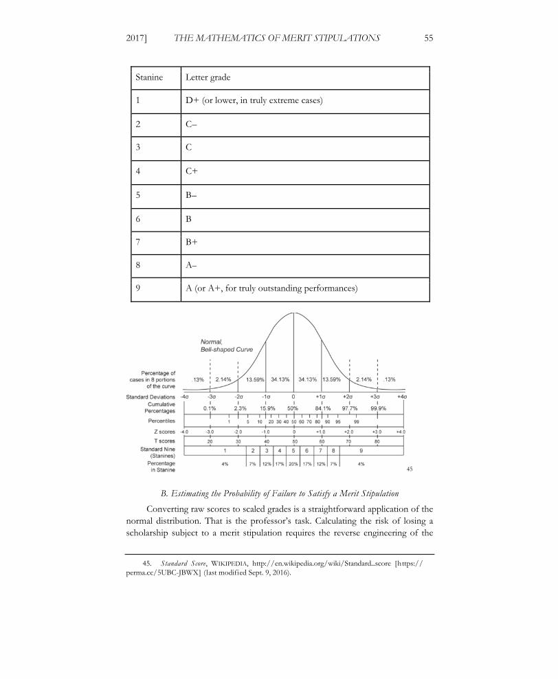
The closely related system of stanines (Standard Nines)42 also works very well with the grading scale I have just described. The United States military historically valued stanines as a way of translating the z-scores of standard scoring, which range across either side of zero, to a scale of single-digit integers from one to nine inclusive.43 To use stanines, divide a Gaussian distribution into nine bands, centered on the fifth band.44 The second through eighth bands each traverse 0.35 standard deviations; the first and ninth stanine cover, respectively, the lowest and highest ends of the distribution. Assigning a B– (2.667) to the fifth stanine and moving one-third of a letter grade in each direction yields the following table of converted grades:

42. See generally ROBERT L. THORNDIKE, APPLIED PSYCHOMETRICS 131 (1982); Stanine, WIKIPEDIA, http://en.wikipedia.org/wiki/Stanine [https://perma.cc/Q7RS-RSAM] (last modified Oct. 20, 2015).

43. Chen, supra note 41. 44. Id.



Stanine Letter grade

1 D+ (or lower, in truly extreme cases)

2 C–

3 C

4 C+

5 B–

6 B

7 B+

8 A–

9 A (or A+, for truly outstanding performances)

45

B. Estimating the Probability of Failure to Satisfy a Merit Stipulation

Converting raw scores to scaled grades is a straightforward application of the normal distribution. That is the professor’s task. Calculating the risk of losing a scholarship subject to a merit stipulation requires the reverse engineering of the

45. Standard Score, WIKIPEDIA, http://en.wikipedia.org/wiki/Standard_score [https://perma.cc/5UBC-JBWX] (last modified Sept. 9, 2016).



grading curve. That is the student’s task. It is certainly possible to approach this assignment in a purely anecdotal, subjective, and nonquantitative way. After years of presumed academic success, every prospective law student has a deep pool of personal experience from which to make a subjective projection of the probability of clearing a GPA hurdle. “I’ve never made below a B in my life,” thinks the student. “How hard can it be to maintain a 3.0 average?”

Therein lies the treacherous trap called the representative heuristic.46 Almost too cavalierly, students project their experiences onto their expectations of legal education. Given the amount of money at stake, to say nothing of the misleading potential of personal experience, students should not approach this assignment without a complete mathematical apparatus. As one of Sean Connery’s movie characters once advised, you shouldn’t “bring[ ] a knife to a gunfight.”47

Because the same curve—the Gaussian distribution—is doing the work, applied mathematics drives both the professor’s task and the student’s task. For any statistical distribution, the probability density function describes the likelihood that a random variable will have a particular value.48 The probability density function (pdf) of a standard normal distribution is:49

Recall the definition of a standard score: . This definition enables us

to restate the pdf of a standard normal distribution in an extremely compact and convenient form—in terms of the mean (μ) and the variance (σ2), or the square of the standard distribution)—of the distribution:

The whole point of this exercise is to determine the parameters μ and σ of the school’s GPA distribution. That task in turn requires us to examine the cumulative distribution function.

The cumulative distribution function (cdf ) describes the probability that a random variable will fall within the interval (–∞, x). In colloquial terms, perhaps the best way to understand the difference between the cumulative distribution function

46. See Daniel Kahneman & Amos Tversky, Subjective Probability: A Judgment of Representativeness, in JUDGMENT UNDER UNCERTAINTY: HEURISTICS AND BIASES 32, 32–33 (Daniel Kahneman, Paul Slovic, & Amos Tversky eds., 1982).

47. Watch THE UNTOUCHABLES (Paramount Pictures 1987). 48. See Probability Density Function, WIKIPEDIA, http://en.wikipedia.org/wiki/Probability_

density_function [https://perma.cc/9D6D-FY3Q] (last modified Jul. 25, 2016). 49. The ensuing discussion draws very heavily from Wikipedia’s article on normal distribution.

Normal Distribution, WIKIPEDIA [hereinafter Normal Distribution], http://en.wikipedia.org/wiki/Normal_distribution [https://perma.cc/LQ93-RAL3] (last visited Apr. 7, 2016).

(x) 1

2e 1

2 x 2

z x

f (x; , 2) 1

x

, 0



and the pdf is to visualize the familiar “bell curve.” Start at the extreme left, at the lowest range of possible values. By reporting the height of the bell curve at any particular value on the horizontal axis, the pdf describes the probability of that value. In this casual, visual sense, the pdf is a one-dimensional value.

By contrast, the cumulative distribution function tallies all the values on the curve as you move left to right, from its lowest extreme toward the highest. It describes the sum of those values as the total area under the curve. Calculating the area under a curve is the aim of integral calculus.50 Intuitively, then, the cdf is computed as the integral of the pdf:

This integral cannot be expressed through elementary functions. Instead, it is

expressed through a special function called the error function, or erf:

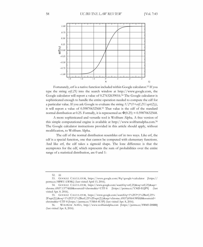
For its own part, computing the error function is a formidable task. Erf is an integral that cannot be expressed through elementary functions:51

Erf takes the form of a sigmoid curve whose asymptotes are ±1:

50. See Integral, WIKIPEDIA, https://en.wikipedia.org/wiki/Integral [https://perma.cc/5Y8G-4CLM] (last modified Aug. 30, 2016).

51. See Error Function, WIKIPEDIA [hereinafter Error Function], http://en.wikipedia.org/wiki/Error_function [https://perma.cc/P4FN-66N9] (last modified Aug. 27, 2016).

(x) 1

2e

t2

2 dt

x

2erf1

2

1)(

xx

erf (x) 2

et 2

dt0

x



52

Fortunately, erf is a native function included within Google calculator.53 If you type the string erf(.25) into the search window at http://www.google.com, the Google calculator will report a value of 0.27632639016.54 The Google calculator is sophisticated enough to handle the entire operation needed to compute the cdf for a particular value. If you ask Google to evaluate the string 1/2*(1+erf(.25/sqrt(2))), it will report a value of 0.59870632568.55 That value is the cdf of the standard normal distribution at 0.25. Formally, it is represented as: Φ(0.25) ≈ 0.59870632568.

A more sophisticated and versatile tool is Wolfram Alpha. A free version of this simple computational engine is available at http://www.wolframalpha.com.56 The Google calculator instructions provided in this article should apply, without modification, to Wolfram Alpha.

The cdf of the normal distribution resembles erf in two ways. Like erf, the cdf is a special function, one that cannot be computed with elementary functions. And like erf, the cdf takes a sigmoid shape. The lone difference is that the asymptotes for the cdf, which represents the sum of probabilities over the entire range of a statistical distribution, are 0 and 1:

52. Id. 53. GOOGLE CALCULATOR, https://www.google.com/#q=google+calculator [https://

perma.cc/8BWU-LW8K] (last visited April 13, 2016). 54. GOOGLE CALCULATOR, https://www.google.com/search?q=erf(.25)&oq=erf(.25)&aqs=

chrome..69i57.13774j0j8&sourceid=chrome&ie=UTF-8 [https://perma.cc/Y36D-EQP9] (last visited Apr. 8. 2016).

55. GOOGLE CALCULATOR, https://www.google.com/search?q=1%2F2*(1%2Berf(.25% 2Fsqrt(2)))&oq=1%2F2*(1%2Berf(.25%2Fsqrt(2)))&aqs=chrome..69i57j69i64.989j0j8&sourceid= chrome&ie=UTF-8 [https://perma.cc/VM64-4U5P] (last visited Apr. 8, 2016).

56. WOLFRAM ALPHA, http://www.wolframalpha.com [https://perma.cc/FBM5-DSRR] (last visited Apr. 8, 2016).



Fx

; , 2

(

x

) 1

21 erf

x 2

F z ; , 2 (z ) 1

21 erf

z

2

57

Like the pdf, the cdf can be expressed in terms of standard scores. Because grades expressed as standard scores are our ultimate objective, it will be useful to expressing the cdf in terms of the standard score, :

Or, even more simply, in terms of z directly:

At this point, it behooves us to pause and admire what applied mathematics can do. If we know the parameters of a law school’s GPA distribution, we can express the probable rank within any class associated with a particular grade. I shall take an example from my own teaching experience. On many occasions, I was instructed to set the mean grade point average in my first-year courses in a range between 2.800 and 2.933. Let us split the difference and stipulate that my value for μ found the sweet spot at the midway point of 2.867. I also found, for reasons that will be obvious to anyone who understands the standard normal distribution, that assigning all but roughly 5% of the grades—combining outliers at both extremes, the worst and the best performances in the class—within the range defined by 0.867 < g < 3.867 generated a standard deviation close to 0.500. Therefore, σ = 0.500. With these parameters, μ = 2.867 and σ = 0.500, we can predict what fraction of my students would have met a merit stipulation of 3.000 or perhaps even 3.250. For any merit stipulation, the cdf for the z-score corresponding to the stipulated

57. Cumulative Distribution Function, WIKIPEDIA, http://en.wikipedia.org/wiki/Cumulative_ distribution_function [https://perma.cc/8XPM-GJZY] (last modified July 29, 2016).

z x



minimum grade point average describes the probability that a student will fail to satisfy that merit stipulation:

Failure rate associated with a merit stipulation =

The following table describes the failure rate corresponding to merit stipulations requiring GPAs of 2.500, 3.000, 3.200, and 3.333, within a law school environment where μ ≈ 2.867 and σ ≈ 0.500. Note that it is crucial to begin by converting each GPA to its corresponding z-score by applying the formula for the standard score, :

Merit stipulation expressed as a grade point average

z-score (standard score):

Predicted failure rate:

2.500 –0.733 23.2%

3.000 0.267 60.5%

3.200 0.667 74.7%

3.333 0.933 82.4%

Each row in the table can be calculated with nothing more than the GPA in question, the parameters μ = 2.867 and σ = 0.500, and either Google calculator or the free version of Wolfram Alpha. Focus on the second row, which expresses a perfectly ordinary merit stipulation that students must meet or beat a GPA of 3.000 in order to retain their financial aid. First, calculate z by submitting this string to Google or Wolfram Alpha:

(3–2.867)/0.5

This should report a value for z of 0.266. In the table, I rounded the value to 0.267, since 2.867 really is 2.866667, carried out to six places after the decimal point. The rounding error ultimately makes little difference. Now submit this value of z for purposes of calculating the cdf, Φ(0.266):

1/2*(1+erf(0.266/sqrt(2)))

z x

(z) 1

21 erf

z

2

(z) 12

1 erf z 2

z x



Google will report a value of 0.60488039548 for Φ(0.266).58 This represents the aggregation of all GPAs from the lowest to a z-score of 0.266, which, given the parameters of this school’s grade distribution, corresponds to a GPA of 3.000. Those who are supremely confident in their ability to count nesting parentheses can compute the predicted failure rate with a single Google calculator operation:

1/2*(1+erf((3 – 2.867)/(.5*sqrt(2))))

All of the foregoing formulas work in Excel as well as Google calculator. Excel does exhibit an additional quirk. The erf function in Excel demands a non-negative argument. Since erf(–x) = –erf(x), the following expression works when μ (the school-wide mean GPA) exceeds x (the merit stipulation), as in the first line of the table above:

1/2*(1–erf((2.867 – 2.5)/(.5*sqrt(2))))

In my experience, law schools seldom disclose the parameters of their grade distributions.59 I suspect that the reason for this failure is that law school administration, let alone the faculty, rarely if ever computes those statistical parameters. In most cases, a school will name the grade point average at which it enforces its merit stipulations, albeit without providing further details about the full distribution of grades, much less targeted information about the mean and the standard distribution.60 In mathematical terms, schools often report x but conceal μ and σ. Recall David Segal’s New York Times story about law school financial aid and merit stipulations: “The University of Florida’s law school requires students to maintain a 3.2 GPA to keep their scholarships; at the Benjamin N. Cardozo School of Law in Manhattan, it’s a 2.95.”61

As a first cut, an applicant hoping to evaluate a scholarship from a school that does nothing beyond defining its merit stipulation can calculate the cdf for a range of values for μ and σ. I will offer one suggestion. The grade of A– tends to fall at or near two standard deviations above the mean. We may begin by assuming that a GPA of 3.667 has a z-score of 2. Since rearrangement of the formula for the standard score defines the standard deviation as the difference between the scaled grade and the mean, divided by the standard score,

58. GOOGLE, https://www.google.com/webhp?sourceid=chromeinstant&ion=1&espv= 2&ie=UTF-8#q=1%2F2*(1%2Berf(.266%2Fsqrt(2)))%3D [https://perma.cc/7RU9-ES6E] (last visited Apr. 4, 2016).

59. See Debra Cassens Weiss, Bait and Switch? Law Schools Gain in US News with Merit Scholarships Conditioned on High Grades, ABA JOURNAL (May 2, 2011, 12:34 PM), http:// www.abajournal.com/news/article/bait_and_switch_law_schools_gain_in_us_news_with_merit_ scholarships_conditi/[https://perma.cc/U6WW-C7VJ].

60. See id. 61. Segal, supra note 2, at BU6.



, we can estimate σ by substituting 3.667 (the GPA value of an A–) for x and

2 for z : .

The following table estimates the failure rates for a range of merit stipulations from 2.8 through 3.2, on the assumption that the school’s mean GPA ranges from 2.667 through 3.333 with a standard deviation corresponding to (3.667 – μ) / 2. Since 47.7% of a standard normal distribution falls between the mean and two standard deviations above the mean (in other words, Φ(2) – Φ(0) ≈ 0.477), one implication of this assumption is that the school assigns 47.7% of its grades between its mean and the grade of A–. Data on honors at graduation may shed light on the validity of this assumption, though its interpretation must be tempered by awareness of survivorship bias (informally, the tendency of “winners” in a competitive process to skew estimates of the likelihood of success).62

μ = 2.8 = 2.9 = 3.0 = 3.1 = 3.2

2.667 0.5000 70.31% 82.47% 90.88% 95.85% 98.36%

2.750 0.4583 58.64% 74.36% 86.23% 93.67% 97.52%

2.833 0.4167 43.64% 62.55% 78.81% 89.97% 96.08%

2.917 0.3750 26.69% 46.46% 67.16% 83.59% 93.46%

3.000 0.3333 11.51% 27.43% 50.00% 72.57% 88.49%

3.083 0.2917 2.60% 10.44% 28.39% 54.55% 78.81%

3.167 0.2500 0.17% 1.64% 9.12% 29.69% 60.51%

3.250 0.2083 0.00% 0.04% 0.82% 7.49% 31.56%

3.333 0.1667 0.00% 0.00% 0.00% 0.26% 5.48%

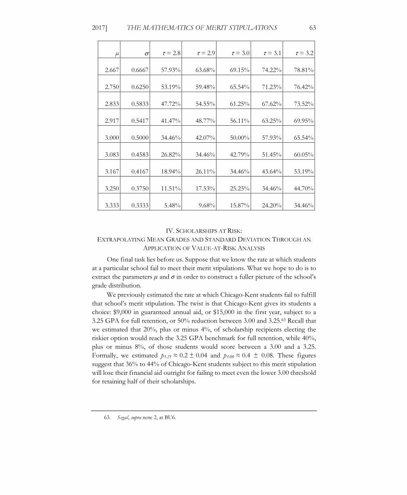
Suppose instead that the distance from the school-wide mean GPA to the

grade of A (4.000) is equivalent to a z-score of 2. This may be a more realistic assumption, in the sense that grades are more widely dispersed from the mean. In that event, the table of failure rates changes rather dramatically:

62. See generally, e.g., Edwin J. Elton, Martin J. Gruber & Christopher R. Blake, Survivorship Bias and Mutual Fund Performance, 9 REV. FIN. STUD. 1097 (1996); Marc Mangel & Francisco J. Samaniego, Abraham Wald’s Work on Aircraft Survivability, 79 J. AM. STAT. ASS’N 259 (1984).

z x

3.667

2



µ = 2.8 = 2.9 = 3.0 = 3.1 = 3.2

2.667 0.6667 57.93% 63.68% 69.15% 74.22% 78.81%

2.750 0.6250 53.19% 59.48% 65.54% 71.23% 76.42%

2.833 0.5833 47.72% 54.55% 61.25% 67.62% 73.52%

2.917 0.5417 41.47% 48.77% 56.11% 63.25% 69.95%

3.000 0.5000 34.46% 42.07% 50.00% 57.93% 65.54%

3.083 0.4583 26.82% 34.46% 42.79% 51.45% 60.05%

3.167 0.4167 18.94% 26.11% 34.46% 43.64% 53.19%

3.250 0.3750 11.51% 17.53% 25.25% 34.46% 44.70%

3.333 0.3333 5.48% 9.68% 15.87% 24.20% 34.46%

IV. SCHOLARSHIPS AT RISK: EXTRAPOLATING MEAN GRADES AND STANDARD DEVIATION THROUGH AN

APPLICATION OF VALUE-AT-RISK ANALYSIS

One final task lies before us. Suppose that we know the rate at which students at a particular school fail to meet their merit stipulations. What we hope to do is to extract the parameters μ and σ in order to construct a fuller picture of the school’s grade distribution.

We previously estimated the rate at which Chicago-Kent students fail to fulfill that school’s merit stipulation. The twist is that Chicago-Kent gives its students a choice: $9,000 in guaranteed annual aid, or $15,000 in the first year, subject to a 3.25 GPA for full retention, or 50% reduction between 3.00 and 3.25.63 Recall that we estimated that 20%, plus or minus 4%, of scholarship recipients electing the riskier option would reach the 3.25 GPA benchmark for full retention, while 40%, plus or minus 8%, of those students would score between a 3.00 and a 3.25. Formally, we estimated p3.25 ≈ 0.2 ± 0.04 and p3.00 ≈ 0.4 ± 0.08. These figures suggest that 36% to 44% of Chicago-Kent students subject to this merit stipulation will lose their financial aid outright for failing to meet even the lower 3.00 threshold for retaining half of their scholarships.

63. Segal, supra note 2, at BU6.



We now face the mirror image of the problem we confronted in the previous section. There, we presumably knew something about a school’s grade distribution or, at the very least, made an informed guess as to the values of the critical parameters, mean and standard deviation. For instance, I gave an example, drawn from my own teaching experience, of a school where the parameters of the grade distribution were set by policy and refined by faculty custom. If you know that μ ≈ 2.867 (as a matter of formal policy) and σ ≈ 0.500 (as a matter of custom), you should expect roughly 60.5% of the students receiving financial aid subject to a merit stipulation will fail to reach the make-or-break GPA boundary of 3.00.

Suppose instead that you know that a third to a half of the students subject to a merit stipulation will lose their scholarships, in part or in whole, after the first year of law school. At the very least, the journalistic efforts of a muckraking New York Times reporter give you good reason to believe that the rate of failure falls somewhere between 36% and 44%.64 You will find it very useful to reverse engineer this school’s mean GPA and its standard deviation. Knowing those parameters unlocks the entire garden of mysteries lying within the Gaussian distribution.

We can tackle this problem with a simplified version of a risk assessment tool used widely in the financial industry: value-at-risk analysis, or VaR.65 Suppose that an investor stakes $1 million on an index fund tracking the Standard & Poor’s 500.66 She asks her financial advisor, “If capital markets go down to an extent witnessed only once in a hundred trading days, what can I lose by tomorrow’s market close?” In its simplest form, VaR analysis assumes normally distributed returns. VaR1% is this quantitative tool’s answer to the investor’s question. An advisor using conventional VaR analysis will report a one-day value of VaR1% as $23,260 for a $1 million portfolio. VaR1% = $23,260 is a fancy, technocratic way of telling this investor that she faces a 1% chance of losing $23,260 or more on her S&P 500 index fund on any given trading day. Global guidelines for regulating systemically important financial institutions have prescribed a version of VaR analysis for assessing banks’ exposure to market risk.67

In other words, despite its flaws and limitations, VaR analysis arguably represents the most important tool for evaluating market risk as one of several

64. See id. 65. See generally LINDA ALLEN ET AL., UNDERSTANDING MARKET, CREDIT, AND

OPERATIONAL RISK: THE VALUE AT RISK APPROACH 1–20 (2004) (providing an introduction to value-at-risk analysis); PHILIPPE JORION, VALUE AT RISK: THE NEW BENCHMARK FOR MANAGING

FINANCIAL RISK (3d ed. 2007). 66. This example is drawn from ALLEN ET AL., supra note 65, at 5–7, and developed at greater

length in James Ming Chen, Measuring Market Risk Under the Basel Accords: VaR, Stressed VaR, and Expected Shortfall, 8 AESTIMATIO 184, 186–89 (2014).

67. See BASEL COMM. ON BANKING SUPERVISION, BANK FOR INT’L SETTLEMENTS, INTERNATIONAL CONVERGENCE OF CAPITAL MEASUREMENT AND CAPITAL STANDARDS: A REVISED FRAMEWORK ¶¶178–81 (2004), http://www.bis.org/publ/bcbs107.pdf [https://perma.cc/S3U8-V4BD]. For further discussion of the Basel Accords and their treatment of VaR and the leading alternative methodology for measuring market risk (expected shortfall), see generally Chen, supra note 66, at 184.



threats to the global financial system. VaR analysis enables financial analysts—in a personal, institutional, or regulatory setting—to estimate what portion of their portfolios may decline over some interval of time.68 Stripped to its essentials, however, VaR operates on the same terms as law school grading. Both exercises in evaluating performance rely on the mathematics of the Gaussian distribution.69 Mathematical analysis of merit stipulations in financial aid boils down to an exercise in VaR, albeit with retail-level sums much smaller than those in most commercial VaR scenarios—and with a vastly higher probability of failure.

It takes very little imagination to realize that a law student accepting financial aid subject to a merit stipulation needs to perform a VaR calculation of her own. The amounts at stake do differ. So do the probabilities. But at the level of mathematical mechanics, the problems are remarkably similar. Applied mathematics does not care whether a problem is smaller in magnitude. Nor does it care whether the problem is more personally intense. Our investor feared a 1% chance of losing 2.326% ($23,260) of her $1 million portfolio. The only difference in the financial aid setting is the amount at risk and the level at which the likelihood of loss becomes critical.

The Chicago-Kent student who accepts a $15,000 scholarship subject to a merit stipulation has every objective reason to know, based on the school’s willingness to guarantee $9,000 a year over three years, that the risk-adjusted value of the financial aid package must be $27,000, or a 40% discount off the hoped-for value of three annual awards of $15,000 each, or $45,000 over three years in law school. The Chicago-Kent College of Law has all but equated these two financial aid packages. It has further divided its merit stipulation into two tiers: partial (50%) loss of a scholarship for a GPA between 3.00 and 3.25, and complete loss for a GPA below 3.00.70 Surely this information enables students to estimate the mean and standard deviation of Chicago-Kent’s grade distribution.

As it happens, the Chicago-Kent inquiry does require more math than the Wall Street problem. Although both problems begin with basic VaR analysis, the law school problem asks us to compute the parameters μ and σ. That, too, we can do. It will take an additional mathematical step.

In generalized, formal terms, VaR for a certain risk or confidence level is the quantile that solves the following equation:71

68. See JORION, supra note 65, at 115. 69. In principle, parametric VaR analysis may be “generalize[d] to other distributions as long as

all the uncertainty is contained in .” JORION, supra note 65, at 113. For applications of VaR analysis using Gaussian and non-Gaussian distributions, compare James Ming Chen, The Promise and the Peril of Parametric Value-at-Risk (VaR) Analysis, 2 CENT. BANK J.L. & FIN. 1, 5–7 (2015) (Gaussian VaR), with id. at 7–17 (Student’s t-distribution), and id. at 18–23 (logistic distribution). Non-Gaussian VaR, to say nothing of nonparametric VaR, lies beyond the scope of this Article. See generally JORION, supra note 65, at 108–10.

70. Segal, supra note 2, at BU6. 71. See Jón Daníelsson & Jean-Pierre Zigrand, On Time-Scaling of Risk and the Square-Root-of-

Time Rule, 30 J. BANKING & FIN. 2701, 2702 (2006).



represents the confidence level. In the case of my hypothetical investor with a $1 million portfolio invested in an S&P 500 index fund, = 0.01. In the case of Chicago-Kent or any other law school subjecting financial aid awards to a merit stipulation, the level of risk at stake, under any set of assumptions, is considerably higher. f(x) refers to the relevant probability density function, whether it involves the distribution of returns on a portfolio or a financial institution, or the distribution of grades in a law school.

Both the Wall Street problem of value at risk in a $1 million portfolio and the goal of discerning the distribution of grades at Chicago-Kent require the computation of statistical quantiles.72 In education, quantiles matter because schools and employers use them ruthlessly to sort students and to make high-impact decisions.73 All sorts of benefits within law school and in the job market, from law review membership and graduation with honors to opportunities to interview with prestigious, high-paying employers, hinge on class rank or membership in a particular quartile, decile, or percentile.

In statistical terms, the quantile function of a distribution is the inverse of the cumulative distribution function. The quantile function of the standard normal distribution is expressed as a transformation of the inverse error function:

In spite of its notation, the inverse error function, or erf–1, is not the reciprocal of the error function, erf. Formally, if somewhat tautologically, erf–1 is defined as the function that satisfies these two identities:74

R represents the set of real numbers. The inverse error function looks like this:

72. Once again, I draw very heavily from Normal Distribution, supra note 49. I have also drawn material from Quantile Function, WIKIPEDIA, http://en.wikipedia.org/wiki/Quantile_function [https://perma.cc/9Z8F-8XXV] (last modified Sept. 9, 2016), and Error Function, supra note 51.

73. See Richard Sander & Jane Bambauer, The Secret of My Success: How Status, Eliteness, and School Performance Shape Legal Careers, 9 J. EMPIRICAL LEGAL STUD. 893, 910–12 (2012).

74. See Inverse Erf, WOLFRAM ALPHA, http://mathworld.wolfram.com/InverseErf.html [https://perma.cc/BB9V-7RZQ] (last visited Apr. 7, 2016).

f (x) dx

VaR

zp 1(p) 2 erf 1(2p 1)

erf[erf 1(x)] x, 1 x 1

erf 1[erf(x)] x, x R



75

Because the quantile function is the inverse of the cumulative distribution function, it is designated as the inverse of the capital phi symbol that designates the cdf: Φ–1( p). Designating the quantile function, alternatively, as zp may help us visualize what we really seek. The quantile zp describes the statistical distance, in multiples of standard deviation , that a standard normal random variable will fall from the mean for a given probability p. Formally: “A normal random variable x will exceed + zp with probability 1 – p and will lie outside the interval ± zp with probability 2(1 – p).”76

More intuitively, perhaps, we can ask what standard score, or z, corresponds to the value of the cdf representing a certain percentage of the total under the curve that defines the pdf. Recall that we defined the failure rate associated with a merit stipulation as the cumulative distribution function of the standardized academic cutoff score—that is, the cdf of the GPA, expressed as a z-score, that defines the merit stipulation:

Algebraic rearrangement to solve for z shows that the solution is in fact the inverse cumulative distribution function of Φ(z ):

75. Inverse Erf, WOLFRAMMATHWORLD, http://mathworld.wolfram.com/InverseErf.html [https://perma.cc/KHL9-RTY9] (last updated Feb. 27. 2017).

76. LEE RAZDOLSKY, PROBABILITY-BASED STRUCTURAL FIRE LOAD 85 (2014); see also F.M. DEKKING, C. KNAAIKAMP, H.P. LOPUHAÄ & L.E. MEESTER, A MODERN INTRODUCTION TO

PROBABILITY AND STATISTICS § 23.2, at 345 (2006); KEVIN J. HASTINGS, INTRODUCTION TO

PROBABILITY WITH MATHEMATICA 220 (2d ed. 2009).

(z ) 1

21 erf

z 2



(z ) 1 2

1 erf z

2

2 (z ) 1 erf z 2

2 (z) 1 erf z 2

At this point, a worked example or two seems in order. The inverse error function, unfortunately, is not readily found on calculators. It is not supported in Google calculator or in Excel. Online inverse erf calculators, however, can be found.77 More straightforwardly, Wolfram Alpha supports inverse erf with the simple command, InverseErf(x), where argument x falls in the range –1 < x < 1.78

Let us begin with our simplified VaR analysis. Recall that we have assumed our investor has staked $1 million in an S&P 500 index fund. The variable VaRp expresses the value at risk given a particular probability of a loss as the product of that probability (p), the total value of the portfolio (v), and –zp.79

The negative sign before –zp allows us to state value at risk as a positive sum at risk of loss. For p = 1% and v = $1,000,000:

All that stands between us and a complete calculation of VaR1% is the value of z1%. That value in turn requires the application of the quantile function:

Inserting this value of z1% into the formula for VaR1% yields a conclusion of VaR1% ≈ $23,260.

Applying the quantile function to Chicago-Kent’s merit stipulation proceeds in similar fashion. Recall that we identified three scenarios representing the range of rates at which Chicago-Kent students would fail to satisfy the merit stipulations

77. At times, I have used the Casio’s “Ke!san” high-accuracy calculation service. KE!SAN

ONLINE CALCULATOR, http://keisan.casio.com/exec/system/1180573448 [https://perma.cc/ XFY3-EC55] (last updated 2017).

78. See, e.g., WOLFRAM ALPHA, supra note 74. 79. See ALLEN ET AL., supra note 65, at 7.

VaRp zp p v

VaRp zp 0.01 $1,000,000

z1% 1(0.01) 2 erf 1[2 0.011] 2.326

z2 e rf 1 [2 (x )1]

z 2 erf 1 [2 (x) 1]



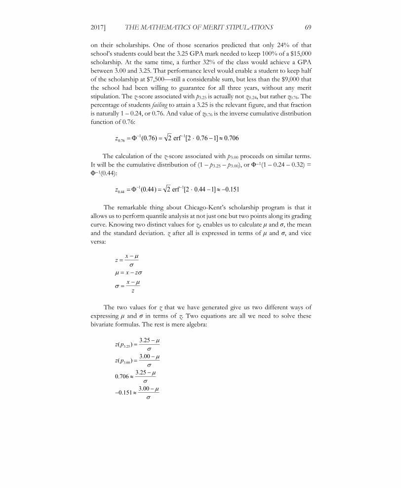
on their scholarships. One of those scenarios predicted that only 24% of that school’s students could beat the 3.25 GPA mark needed to keep 100% of a $15,000 scholarship. At the same time, a further 32% of the class would achieve a GPA between 3.00 and 3.25. That performance level would enable a student to keep half of the scholarship at $7,500—still a considerable sum, but less than the $9,000 that the school had been willing to guarantee for all three years, without any merit stipulation. The z-score associated with p3.25 is actually not z0.24, but rather z0.76. The percentage of students failing to attain a 3.25 is the relevant figure, and that fraction is naturally 1 – 0.24, or 0.76. And value of z0.76 is the inverse cumulative distribution function of 0.76:

The calculation of the z-score associated with p3.00 proceeds on similar terms. It will be the cumulative distribution of (1 – p3.25 – p3.00), or Φ–1(1 – 0.24 – 0.32) = Φ–1(0.44):

The remarkable thing about Chicago-Kent’s scholarship program is that it allows us to perform quantile analysis at not just one but two points along its grading curve. Knowing two distinct values for zp enables us to calculate μ and σ, the mean and the standard deviation. z after all is expressed in terms of μ and σ, and vice versa:

The two values for z that we have generated give us two different ways of expressing μ and σ in terms of z. Two equations are all we need to solve these bivariate formulas. The rest is mere algebra:

z0.76 1(0.76) 2 erf 1[2 0.76 1] 0.706

z0.44 1(0.44) 2 erf 1[2 0.44 1] 0.151

z x

x z

x

z

z(p3.25) 3.25

z(p3.00) 3.00

0.706 3.25

0.1513.00



Subtracting the second equation from the first eliminates the final addend,

. This leaves a simple formula for σ, after which it is easy to insert values for σ

and z to calculate μ:

By performing similar analysis for other values for p3.25 and p3.00, we can generate a table of possible values for μ and σ:

p3.25 P3.00 Φ–1(1–p3.25) Φ–1(1–p3.25–p3.25) μ

0.24 0.32 0.706 –0.151 3.044 0.292

0.20 0.40 0.842 –0.253 3.057 0.229

0.16 0.48 0.994 –0.358 3.067 0.185

The range of plausible values for μ is incredibly tight. The mean GPA at Chicago-Kent is almost certainly in the neighborhood of 3.05. The standard deviation calculation, however, covers a much wider range. Deciding which of these possible values is closest to the actual value of σ demands the application of experience and instinct beyond the purely mathematical aspects of this exercise. We can now use the scaled grade at two standard deviations (multiples of σ) above the mean to evaluate the plausibility of our assumptions. The first row generates a value for z = μ + 2σ at 3.628. This is more credible than the supposition that 3.515 or 3.437 would mark the ninety-eighth percentile (give or take) of grades at Chicago-Kent or, for that matter, any other law school. It is therefore reasonable to surmise that Chicago-Kent’s mean GPA is 3.044, with a standard deviation of 0.292. Formally, μ ≈ 3.044; σ ≈ 0.292.

The foregoing exercise demonstrates that even modest disclosures of information by schools can enable prospective students to conduct a more accurate evaluation of financial aid awards that are contingent upon the maintenance of a particular grade point average. To reach this conclusion, however, I had to deploy value-at-risk analysis (albeit in a relatively simple form), a quantitative tool used by financial institutions and their regulators.

0.857 0.25

0.292

x z 3.25 0.706 0.292

3.00 (0.151 0.292)

3.044



The subtext of this Article, which I shall make clear as I conclude, is that law schools have all but buried the information that would permit prospective students to make fully informed decisions about their professional education and the financial burdens they may have to bear. Parametric VaR analysis lies beyond the quantitative skills of most law school deans and professors.80 It is a bit rich—both in the sense of rich as affluent and rich as ironic—for law schools to shift the risk of conditional financial aid awards onto students, when the tools needed to evaluate the true value of such awards lie beyond the competence of most schools’ faculty and administration.

CONCLUSION

As the twin forces of competition and technology tighten their grip on the legal services industry in the United States, the personal return on investment in legal education continues to decline. The fall may yet become more precipitous than law schools can bear.81 In the meanwhile, however, the very existence of financial aid subject to merit stipulations, to say nothing of the rapid spread in this practice among American law schools, suggests that law schools are willing to shift squarely to their students the bulk of the economic risk inherent in entering their profession. Although this Article can do little to arrest these trends, it does seek to give prospective law students a fuller set of mathematical weapons with which to evaluate the economic landscape of American legal education. Whatever its intangible benefits, legal education ultimately must earn its keep in the form of enhanced future earnings at a price that students can afford here and now.82 At a minimum, this Article should enable students to evaluate more accurately the real value of a scholarship that is contingent upon satisfaction of a merit stipulation.

80. This tool figures prominently in JAMES MING CHEN, POSTMODERN PORTFOLIO THEORY: NAVIGATING ABNORMAL MARKETS AND INVESTOR BEHAVIOR 236–325 (2016); JAMES MING

CHEN, FINANCE AND THE BEHAVIORAL PROSPECT: RISK, EXUBERANCE, AND ABNORMAL

MARKETS 266–71 (2016). 81. See generally BRIAN Z. TAMANAHA, FAILING LAW SCHOOLS (2012). 82. See generally Chen, supra note 7.

scholarships at risk: the mathematics of merit

Documents