I ,,,os..T. 81 -o5 88

FLUID, THERMAL AND AEROSPACE SCIENCES

'DTIC

ELECTEJUL 28 18

DEPARTMENT OF MECHANICAL AND AEROSPACE illII CASE INSTITUTE OF TECHNOLOGY

SCASE WESTERN RESERVE UmNESITYUNIVERSITY CIRCLE * CLEVELAND, I1,0.44106.,

2A, 0V24 O1 wwuutfb~gg

~M~flsu2

TT RAMI

r'TIC TAB ,. ,93

J,,, f€€.

J tii.ton/___.

-Di s t r j oil/

I'RELIMINARY EXPERIMENTAL STUDY OF DISTURBANCES IN A

LAMINAR BOUN1)ARY-LAYER DUE TO

DISTRIBUTED SURFACE ROUGHNESS

by

Leon Leventhal and Eli Reshotko

Department of Mechanical and Aerospace Engineering

CASE WESTERN RESERVE UNIVERSITY '- " "

May 1981 1981j UL 3 18

Approved for public release; distribution umlimited D

i I

IiI

Qualified requestors may obtain additional copies from the Defense

Technical Information Service.

Conditions of Reproduction

Reproduction, translation, publication, use and disposal

in whole or in part by or for the United States Government

is permitted.

...

THIS DOCUMENT IS BEST QUALITY AVAILABLE. THE COPY

FURNISHED TO DTIC CONTAINED

A SIGNIFICANT NUMBER OF

PAGES WHICH DO NOT

REPRODUCE LEGIBLYo

F. ~UNCLASSIFIED _____

SECURITrY Ci S ASS ICATION3 OF TFI' PACE (Wh-i !).1,,t,

REPORT DOCUMENTATION PACE RE.AD INSTRIIChroNS11.I-I)RE f ')NIPLET.IN(.1H

__ANUPiBF R .8 AC58. ',SION NOi 3 RFf 1IFNT , (ATAI, 0", NtjII R

4. TTLF(.r S~tite) TYPL OF REPORT & Pf RIOD COVERED

PRELIMINARY-EXPERIMENTAL ,ST1bY OF -DISTRBANCES IN/A U\AMINAR _BOUNDARY-LAYER D5uE TO DI TRIBLTE1)""/ 44SURF~ACE ROVUGHNESS* " 6.PRORMING 030G. RZPORT Nmr

YAUTHOR(n' B CONTRACT OR GRANT NUMBFERj,)

LEON -LEVENThTATFLI RESH1OTKO 1 AFAR-78-3562 t

9 PkRFORMING OYGANIZA-:rN NAME AND ADDRESS 10 PROGRAM ELEMENT.'PROJECT, TASKAREA 6 W ORK UNIT NUMBERS

CASE WESTERN URESERUE UNIVERSITY .

DEPARTMNT OF MECIHANICAT, & AEROSPACE ENGINEERING ~'2307/A2 /7~CL VFLAND OH 441(, 61102FICONTPOLLING ,>F FICLh N AM!- ANO ADDRESS 12- REPORT DATE

I TT FORCE OFFICE OF SCiENTTFIC RESYARCH /NA // av 1981JjOLLING AFB, 1W~ 2033213NME PFAf.A

4 M (NV0NNu AOF N'>' N AMt 8 AOORFS, i~,r I r~, fifi.1 "i. Ui'I S. EURITY CLASS. (0f ,,1 -t,

q ~ +UNCLASSIFIED15i- OF'CLASSIFICATION U)OWNO-RAL)Nt,

6 0ST lI,,TON STA-LMENT '-f !hi, H~p-tr)

Approved for pub ic release; distribution i ili~ite1

R 015'! P -TRUT IN 5'. ATCMFVN- -.) 9th.. _lv , -n ti f Im (?f.A 2u, f 'If''ilIron Rep-0(

Pt ,.JP .NTAP'/ NOTf

A" . . . . . . . . *. .... h-

Ill F ' 1w.f 1', ' , .RU low4 Speed WinId I ItII 11 1 tlin, I1 1~L~ -Wi I-C aineiiomiet I v.

colkict(t wdi :i setplate anid wi Lh two d i ferent g~rades of' sand-papet I t. ; !it wiiLi a vandpaper covering, giving Re,,, valuies centered

aro0! i W an," kyf Ii coa rser sandpaper 1lavi og Rek, valuies of abot 1,50.

The f1.1W ;ndicated B~lasius profiles for the smooth plate andW i I) T'Wr '61"w' . ',-itli the coarser roughness, the profile was bestA PPr,:x ide ":( .-I o ;- orcfi c at ',be early' stations biit then progressed

DD ,473 .. ,. ' , UNCLASSIFIED /M~ ,(4

I C P C, ASSIri' A' Or .1' pS AGE 'Wte. IWO F,,.d,

UNCLASSIFIEDSECURITY CLASSIFICATION OF THIS PAGE(Iflhem Date Entered)

toward a turbulent profile. The finer surface roughness (Rek 1 10) had only avery slight effect on the u~ms distributions relative to those for a smoothplate. This showed up primarily through examination of the distribution of localturbulence intensity, u'rms/a , which proved to be a much more sensitive indicatotthan dimensionless turbulent energy, "2 2 For the coarser roughness

urms/Uer(Rek , 150), local u'ms intensities in the boundary layer of the order of 5%were observed before the mean profile departed from a Blasius shape. Theprogression toward turbulent mean velocity profiles was accompanied by largeincreases in turbulent intensities over the whole boundary layer but especiallynear the wall. A study of disturbance spectra for this case shows largestamplitudes and amplifications at frequencies well below the Blasius neutralcurve. The maximum amplification rates are about three times those forTollmien-Schlichting instability over a smooth plate. Transition occurs atRex 350,000 which is much below that for a smooth plate.

UNCLASSIFIED

SECURITY CLASSIFICATIO N Of T11 PA F,(fW h1., I['r' t-llf--f,

ABSTRACT

Mean flow and disturbance measurements have been made on a flat

plate model, one meter long in the CWRU low speed wind tunnel using

hot-wire anemometry. Tests were conducted on a smooth plate and with

two different grades of sandpaper covering; first with a sandpaper

covering giving Re values centered around 10 and then with a coarserk

sandpaper having Rek values of about 150.

The mean flow measurements indicated Blasius profiles for the

smooth plate and with the finer roughness. With the coarser rough-

ness, the profile was best approximated by a Blasius profile at the

early stations but then progressed toward a turbulent profile.

The finer surface roughness (Rek 1 10) had only a very slight

effect on the L' distributions relative to those for a smoothrms

plate. This showed up primarily through examination of the distri-

bution of local turbulence intensity, u' /u, which proved to be a

rms

much more sensitive indicator than dimensionless turbulent energy,

U'2 /12 . For the coarser roughness (Re, z 150), local u' intensi-rms C rms

tics in the boundary layer of the order of 5% were observed before

thle mean profile departed from a Blasius shape. The progression

toward turbulent mean velocity profiles w:is accompanied by large

increases in turbulent intensities over the whole boundary layer but

especially near the wall. A study of disturbance spectra for this

ii

case shows largest amplitudes and amplifications at frequencles well

below the Blasius neutral curve. The maximum amplification rates

are about three times those for Tollmien-Schlichting instability

over a smooth plate. Transition occurs at Rex 350,000 which is

much below that for a smooth surface.

4

I

iii

f

ACKNOWLEDGEMENTS

The authors wish to thank Dr. Yasuhiro Kamotani for his very

important help with the hot-wire instrumentation. Special thanks

are also due to Mr. Mike Marhefka for his help concerning equipment

design and maintenance, and to Mrs. Helena Mencl for typing this

report.

This work was supported by the U.S. Air Force Office of

Scientific Research.

iv

TABLE OF CONTENTS

Page

ABSTRACT ii

ACKNOWLEDGEMENTS iv

TABLE OF1' CONTENTS v

LIST OF FIGURES vii

CHAPTER I - INTRODUCTION 1

CHAPTER II - TEST FACILITIES 6

2.1 Low Speed Wind Tunnel 6

2.1.1 Physical Description 6

2.1.2 Calibration 6

2.2 Flat Plate Model 6

2.2.1 The Plate 6

2.2.2 The Mounting 72.2.3 Roughness 8

2.3 Measuring Equipment 9

2.3.1 Pitot-Static Tube 9

2.3.2 Hot Wire 10

2.3.3 Traverse Mechanism 13

2.3.4 Spectrum Analyzer 14

CHAPTER III - EXPERIMENTAL PROCEDURE 15

3.1 Calibration 15

3.2 Smooth Plate 15

3.2.1 Adjustment of Zero Pressure Gradient 15

3.3.2 Measurement of Mean and Fluctuating 17Informat ion

3.3. Rough Plate 18

V

IPage

3.3.1 Additional Adjustments 18

3.3.2 Measurements Taken with Each of the Two 19

Sandpapers

CHAPTER IV - RESULTS AND DISCUSSION 21

4.1 Smooth Plate 21

4.2 Distributed Roughness of Re, (X = 30 cm) = 10.6 22

4.3 Distributed Roughne,-s of Rek (X 30 cm) = 155 24

4.3.1 Mean and Fluctuation Measurements 24

4.3.2 The Spectrum 29

4.3.3 Filtering 31

4.4 Leading Edge of the Distributed Roughness 32

CHAPTER V - SUMMARY AND CONCLUSIONS 34

REFERENCES 36

FIGURES 38

i

AIp FORCE OFFICE Op nCIENTIFIC RESARCH (APSC)

NOTICE OF tAMITTA TO DDCTh!3 teohnical rep'rt has been reviewed eIud (s

.approv:d for pulIc rtleate IkW AFR 19-1.2 (lb)VIDivtril.inTl is u.Dl.IteL.~~~A. D. L':"

I

LIST OF FIGURES

Figure Page

I Schematic diagram of effect of distributed 38rougness on transition on a flat plate

2 The mean velocity distortion due to 2-D rough- 38ness element

3 View of wind tunnel looking upstream toward 39entrance

4 Side view of test section with plate installed 39

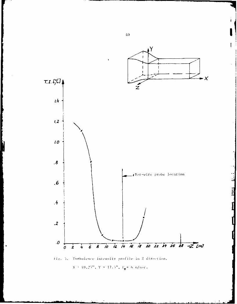
5 Turbulence intensity profile in Z direction 40X = 49.25", Y = 17.5", Ue = 6 m/sec.

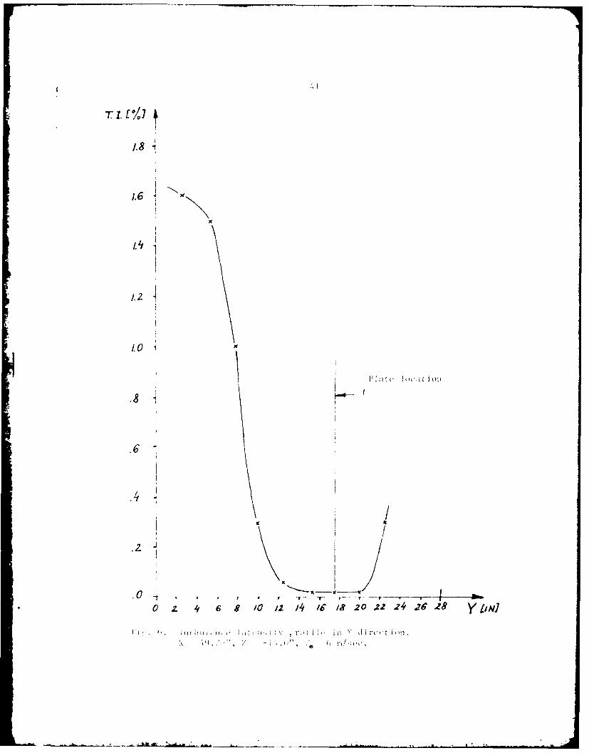
Turbulence itrtensity profile in Y direction 41X - 49.25", Z =-14.0", Ue

= 6 m/see.

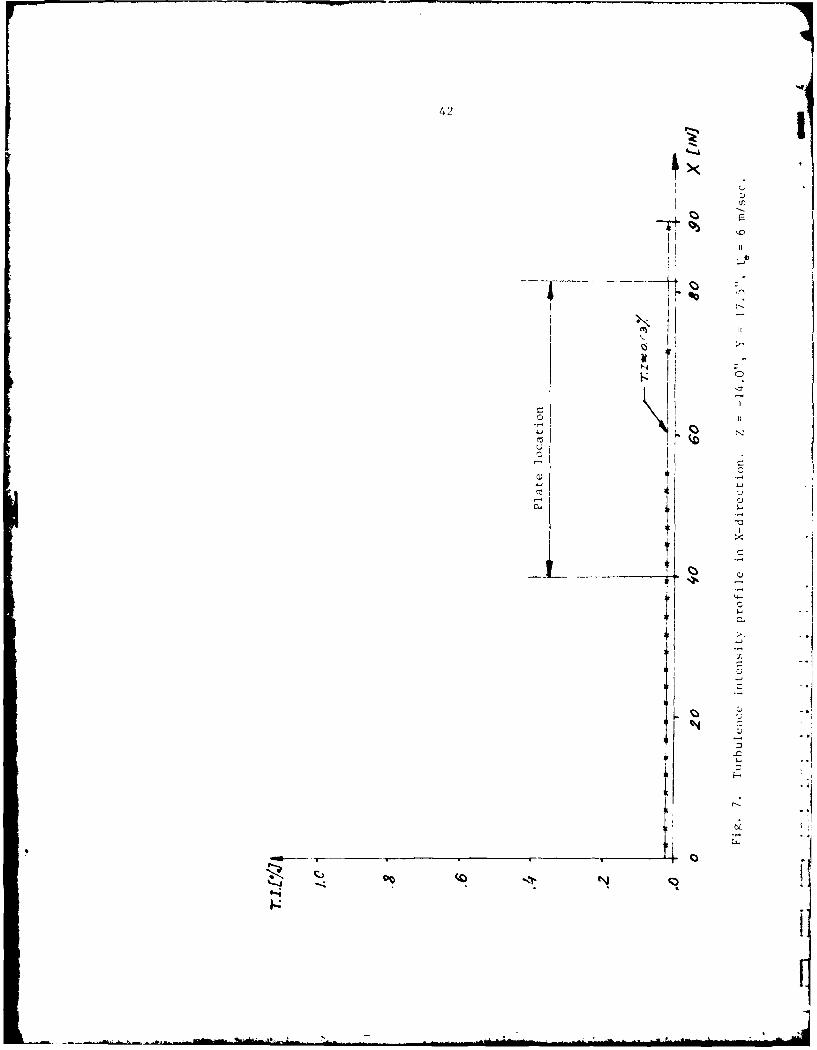
7 Turbulence intensity profile in X-direction 42

Z -14.0", Y = 17.5", Ue = 6 m/sec.

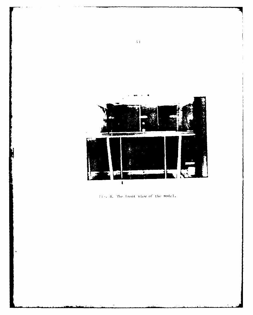
9 The front view of the model 43

9 General view of the model with sandpaper 44

) llot-wire probe and pitot tube over smooth plate 44

II Plate vibrations at Ue = 6 m/sec. 45

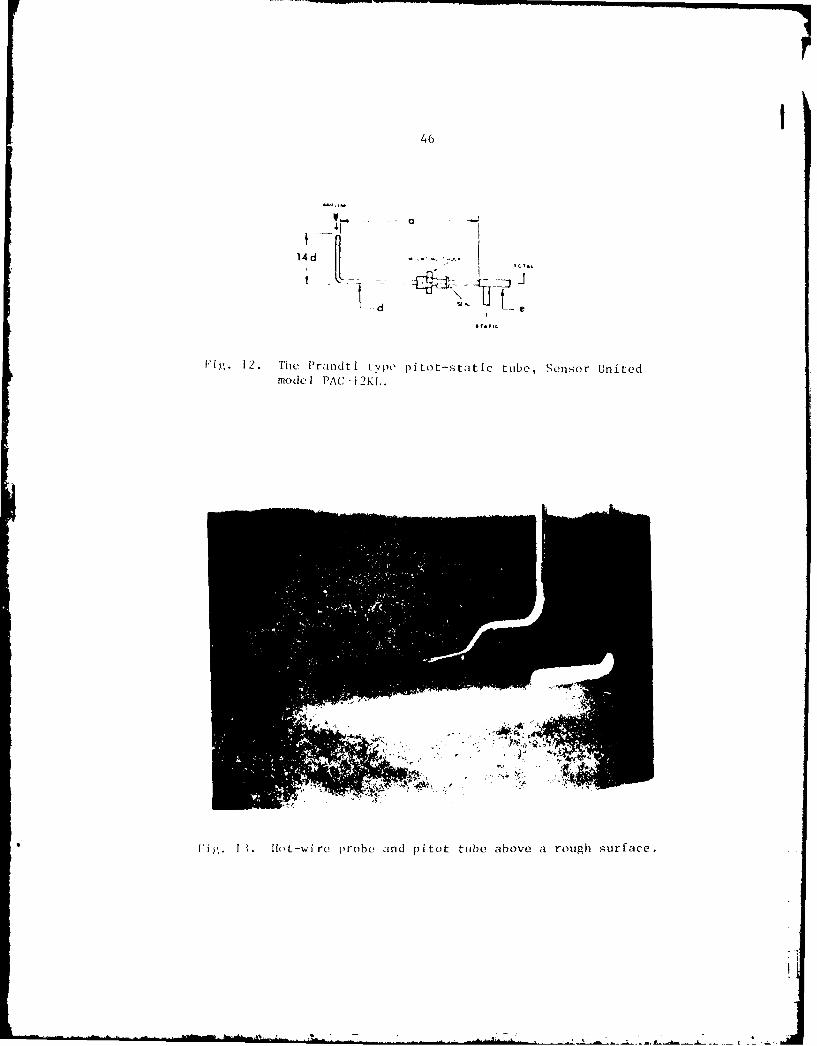
12 The Prandtl type pitot-static tube, Sensor 46United model PAC-12 KL

13 Hot-wire probe and pitot tube above a rough 46,surfac,

14 Flow regimes about unheated circular cylinders 47of high length-to-diameter ratio versusReynolds number

15 The hot-wire anemometer (Shapiro & Edwards, 48model 50), and Meriam manometer

I

Figure Page

16 A close up of the hot-wire probe during the 48

etching process

17 The hot-wire probe in the process of the hot- 49

wire etching

18 The top view of the test section with the tra- 49

versing mechanism

19 Hot-wire calibration curve 50

20 Pressure coefficient for the plate at 0' angle 51

of attack

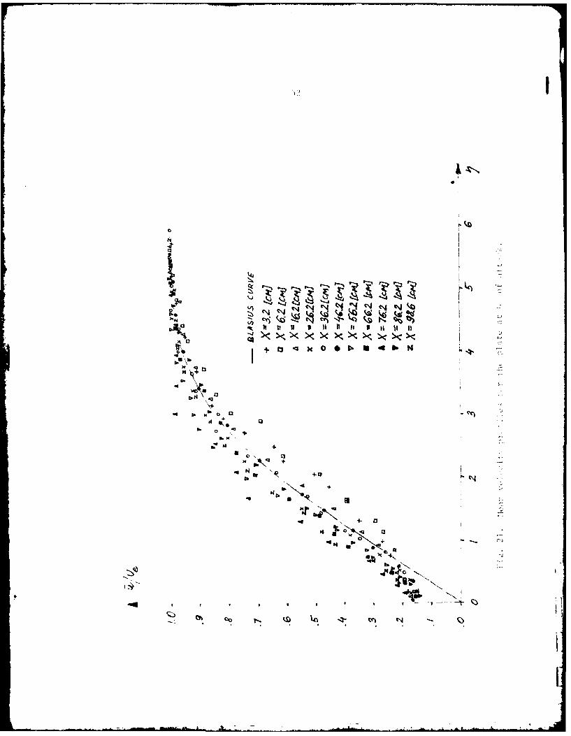
21 Mean velocity profiles for the plate at 00 52

of attack

22 Pressure coefficient for the plate tilted at 53I' angle of attack

23 Mean velocity profiles for the plate tilted at 54

10 angle of attack

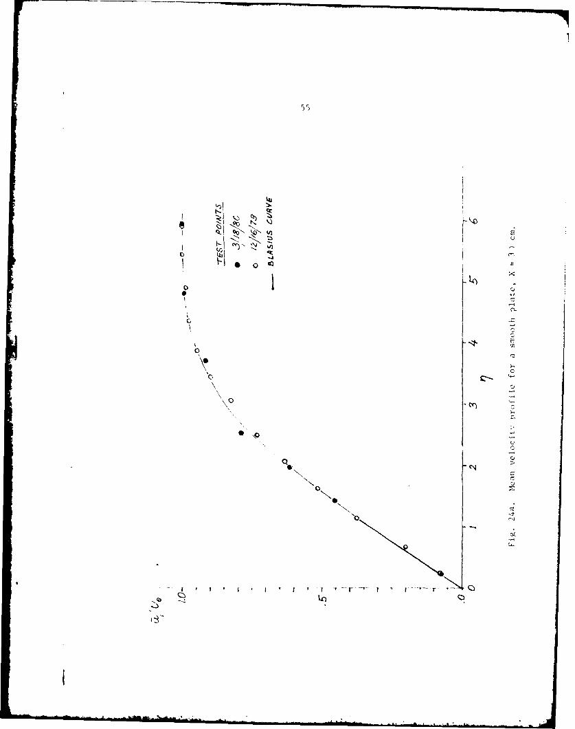
24a Mean velocity profile for a smooth plate, 55

X = 30 cm

24b Mean velocity profile for a smooth plate, 56

X = 40 cm

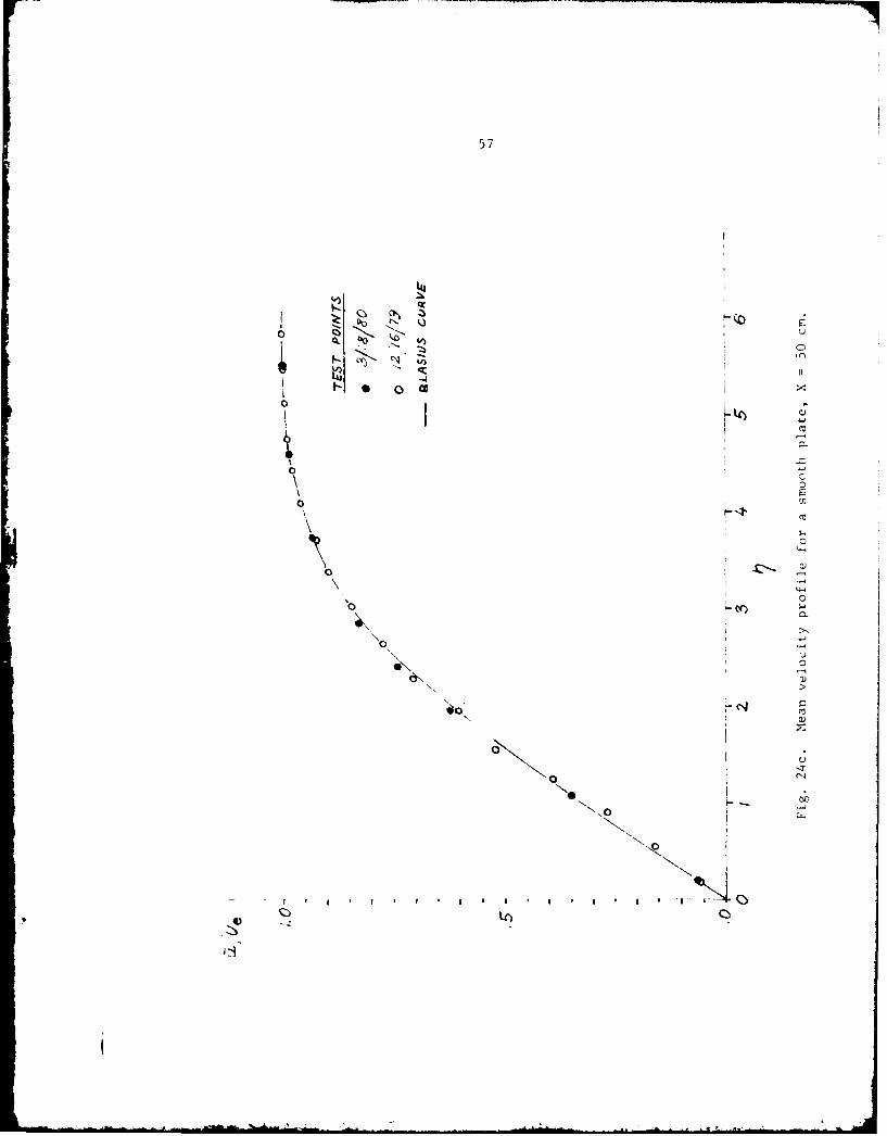
24c Mean velocity profile for a smooth plate, 57X = 50 cm

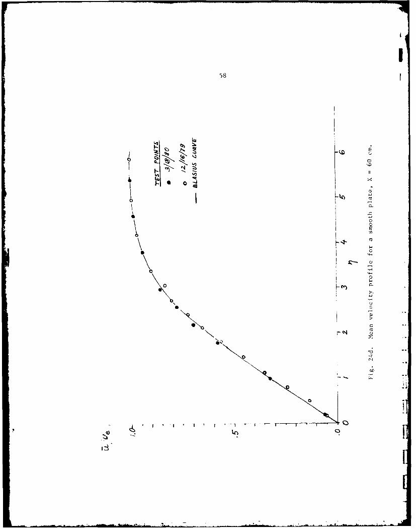
24d Mean velocity profile for a smooth plate 58X = 60 cm

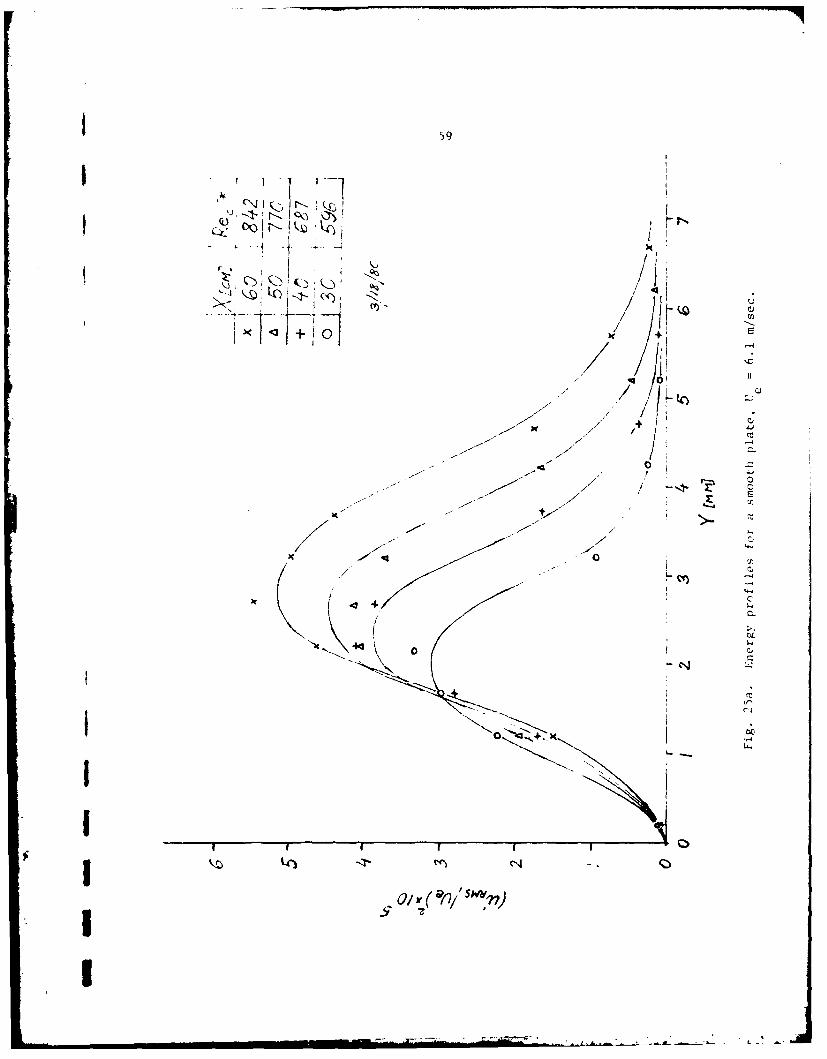
25a Energy profiles for a smooth plate, 59Ue = 6.1 m/sec.

25b Energy profiles for a smooth plate, 60Ue = 6.1 m/sec.

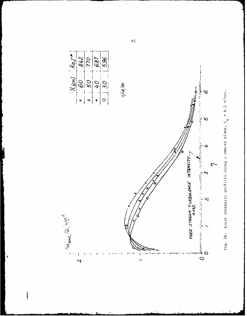
26 Local intensity profiles along a smooth plate, 61Ue = 6.1 m/sec.

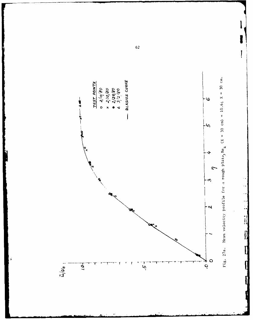
27a Mean velocity profile for a rough plate, 62Re k (X = 30 cm) = 10.6; X = 30 cm

viii

!

F i gure Page

27b Mean velocity profile for a rough plate 63Rek (X = 30 cm) = 10.6; X = 40 cm

27c Mean velocity profile for a rough plate, 64Rek (X = 30 cm) = 10.6; X = 50 cm

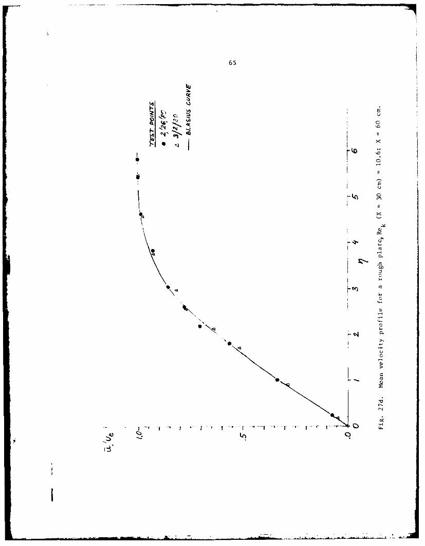
27d Mean velocity profile for a rough plate, 65Rek (X = 30 cm) = 10.6; X = 60 cm

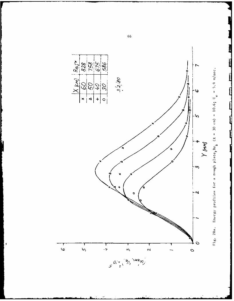
28a EInergy profiles for a rough plate, 66Rek (X = 30 cm) = 10.6; Ue = 5.9 m/sec.

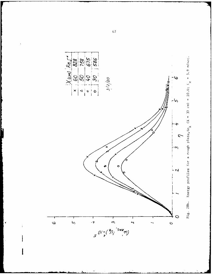
28b Energy profiles for a rough plate, 67Rek (X = 30 cm) - 10.6; Ue = 5.9 m/sec.

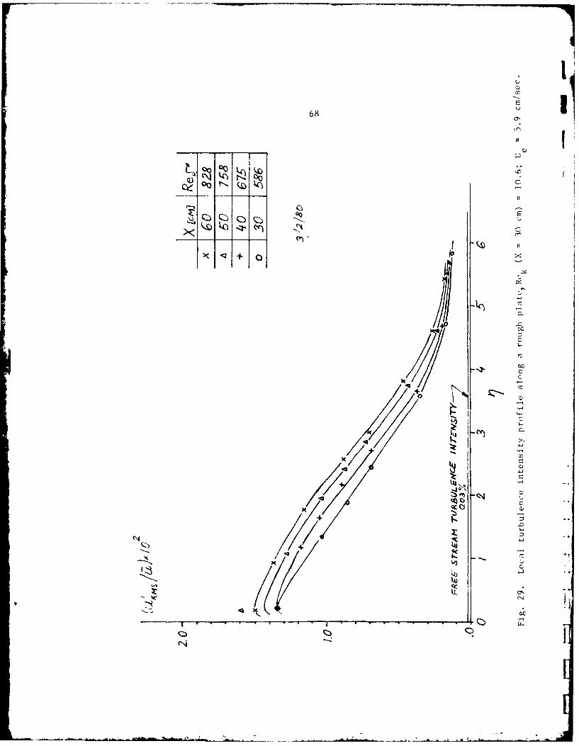
A9 loca l tuirbulence intensity profile along a rough 68plate, Re (X = 30 cm) = 10.6; Ue 5.9 cm/sec.

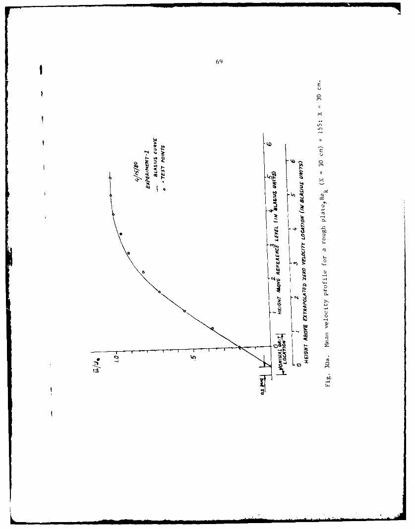
30a Mean e1 locI itV profile for a rough plate, 69Rek (X = 30 cm) 155; X = 30 cm

lOb Mean vefocity profile for a rough plate. 70Rek (X = 31) cm) 1 J55; X = 40 cm

Ok Mean velocity profite for a rough plate, 71Rek (X = 30 cm) 155; X = 50 cm

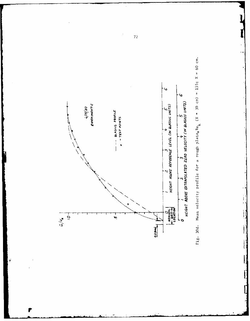
ed NAn1 velOcity profile for a rough plate, 72Rek (X 30 cm) 15; X = 60 cm

IIa Test I - Energy prof iles for a rough plate 73Rek (X '30 cm) 155

3]lb Tes t I1 - Energy profiles for a rough plate, 74Rek (X = 30 cm) = 155

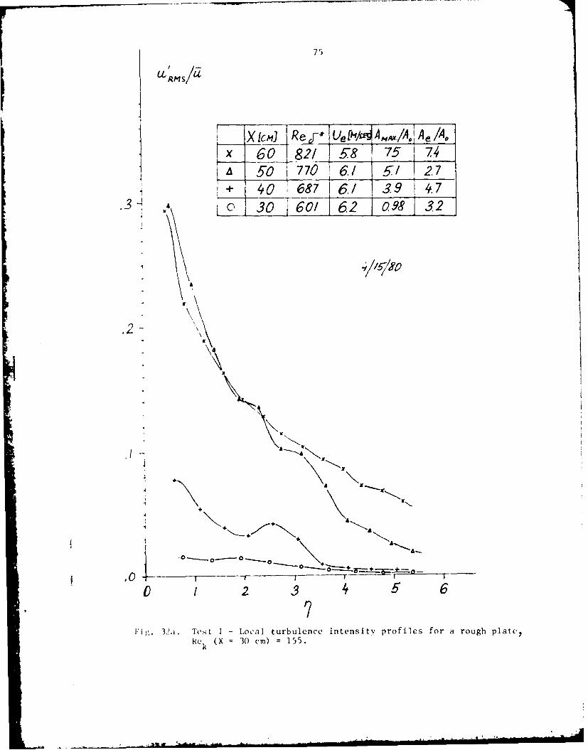
32a Test I - Local I torbu ence intens i ty prof i les for 75

a rough plate, Rek (X = 30 cm) = 155

2Test II - Turbulence intensity profiles for a 76rough plate, Re k (X = 30 cm) = 155

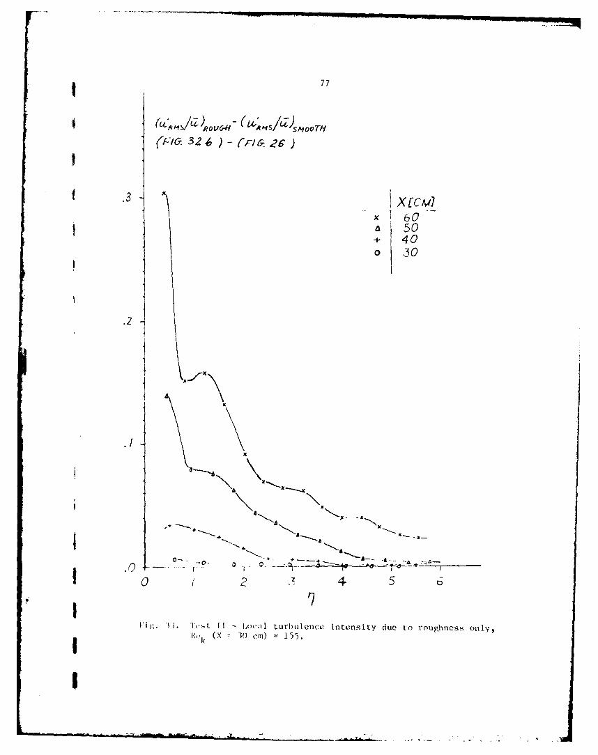
33 Test TI - Local turbulence intensity due to 77 Iroughness only, Rek (X = 30 cm) = 155

ix

Figure Page

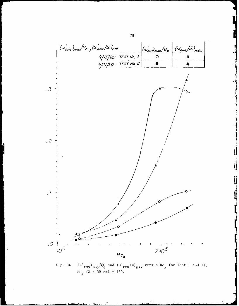
34 (u' rms) max /Ue and (u'rms/U)max versus Rex 78

for Test I and TI, Rek (X = 30 cm) 155tk

35 Spectrum at X = 20 cm, Y = 1.0 mm, 79Rek (X-= 30 cm) 155

36 Spectrum at X = 30 cm, Y 1.5 m, 79

Rek (X = 30 cm) 155

37 Spectrum at X = 40 cm, Y 1.7 mm, 80Rek (X = 30 cm) - 155

38 Spectrum at X = 50 cm, Y = 1.75 mm, 81

Rek (X = 30 cm) - 155

39 Spectrum at X = 60 cm, Y = 1.25 mm, 81Rek (X = 30 cm) - 155

40 Amplitudes of disturbances with frequencies from 82

4.3 Hz to 17.2 Hz versus X" Rek (X = 30 cm) = 155

41 Amplification rates v'rsus X,for disturbanc-s with 83frequencies from 4.3 Hz to 17.2 Hz;Rek (X = 30 cm) 155

42 Amplification rate versus frequency for a con- 84stant Re, in the 4.3 Hz to 17.2 Hz band;Rek (X = 30 cm) 155

43 The highest amplification rate versus X. 85Re k (X = 30 cm) = 155

44 Amplification rate versus frequency for 86Re , = 764, X = 50 cm, Rek (X = 30 cm) = 155

45 Neutral stability results 87

46 Energy content for three frequency bands at the 88location of the maximum total energy,Rek (X = 30 cm) 155

x

II

CHAPTER I

INTRODUCTION

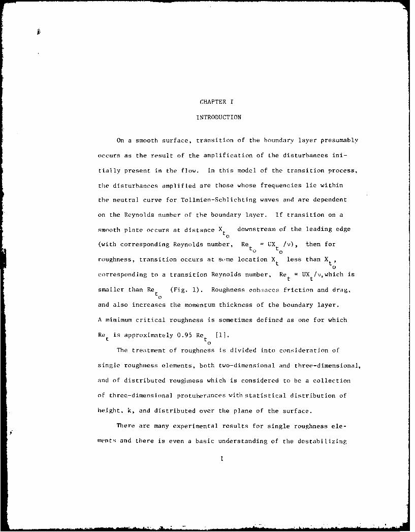
On a smooth surface, transition of the boundary layer presumably

occurs as the result of the amplification of the disturbances ini-

tially present in the flow. In this model of the transition process,

the disturbances amplified are those whose frequencies lie within

the neutral curve for Tollmien-Schlichting waves and are dependent

on the Reynolds number of the boundary layer. If transition on a

smooth plate occurs at distance X downstream of the leading edgeto

(with corresponding Reynolds number, Re = UX /), then fort. t

roughness, transition occurs at sme location Xt less than Xt0

corresponding to a transition Reynolds number, Ret = UX t/v,which is

smaller than Re (Fig. 1). Roughness enh;tnccs friction and drag,t0

and also increases the momentum thickness of the boundary layer.

A minimum critical roughness is sometimes defined as one for which

Re is approximately 0.95 Re [1].t t0

The treatment of roughness is divided into consideration of

single roughness elements, both two-dimensional and three-dimensional,

and of distributed roughness which is considered to be a collection

of three-dimensional protuberances with statistical distribution of

height. k, and distributed over the plane of the surface.

There are many experimental results for single roughness ele-

ments and there is even a basic understanding of the destabilizing

I

2

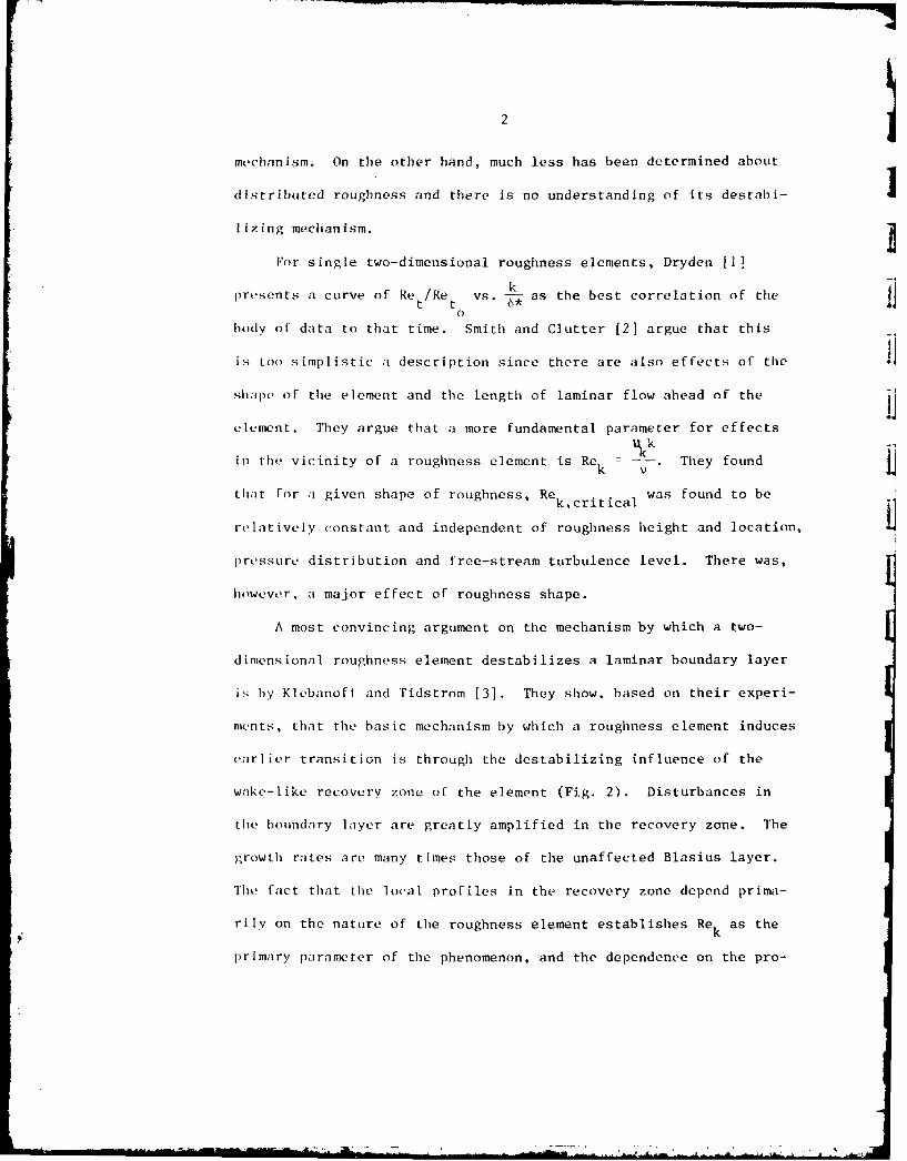
mechanism. On the other hand, much less has been determined about

distributed roughness and there is no understanding of its destabi-

lizing mechanism.

For single two-dimensional roughness elements, Dryden [1

presents a curve of Re /Re vs. -" as the best correlation of the0

body of data to that time. Smith and Clutter [2] argue that this

is 1oo simplistic a description since there are also effects of the

shape of the element and the length of laminar flow ahead of the

element. They argue that a more fundamental parameter for effects

in the vicinity of a roughness element is Rek -V They found

that for a given shape of roughness, Rek,critical was found to be

relatively constant and independent of roughness height and location,

pressure distribution and free-stream turbulence level. There was,

howevr, a major effect of roughness shape.

A most convincing argument on the mechanism by which a two-

dimensional roughness element destabilizes a laminar boundary layer

is by Kiebanoff and Tidstrom [3]. They show, based on their experi-

ments, that the basic mechanism by which a roughness element induces

earlier transition is through the destabilizing influence of the

wake-like recovery zone of the element (Fig. 2). Disturbances in

the boundary layer are greatly amplified in the recovery zone. The

growth rates are many times those of the unaffected Blasius layer.

The fact that the local profiles in the recovery zone depend prima-

rily on the nature of the roughness element establishes Re as thek

primary parameter of the phenomenon, and the dependence on the pro-

3

perties of the parent flow is very weak.

For three-dimensional roughness elements, the critical values

of Rek are higher than for two-dimensional roughness but the desta-

bilizing mechanism may be similar in that disturbances can be great-

ly amplified by the wake-like unstable profiles downstream of the

elements.

In view of the results for single roughness elements and the

known sensitivity of boundary layer stability to small profile

chailges, the analytic investigations to date of distributed roughness

are all based on the premise that distortion of the mean flow by the

roughness enhances instability and leads to earlier transition.

Singh and Lunley [4] made calculations to find the roughness

induced mean velocity profile which they expressed in terms of the

spectral density of the roughness and an influence function. The

resulting profile had an inflection point deep in the inner viscous

region and in their opinion does not contribute to instability.

Outside the wall region, the profile they obtained is more stable

since the curvature in the vicinity of the critical layer has been

increased. Since experimentally, roughness leads to earlier tran-

sition, Singh and Lumleyargue that even if the profile is more

stable, the roughness also introduces disturbances with energy at

wavenumbers to which the profile is unstable.

Lessen and Gangwani [5] model the problem by introducing a wavy

wall to represent one component of the roughness spectrum. The

equation for this roughness induced disturbance is the Orr-Sommerfeld

AL

4

equation with phase velocity equal to zero, but with a non-homoge-

neots boundary condition at y = 0. They retained the Reynolds

stress term in their mean flow equation and so calculated the dis-

torted mean flow. Once this distorted profile was found, the stabi-

lity of this new profile was examined and its critical Reynolds

number calculated. The new profile displayed a point of inflection

near the wall. The new profile was found to be slightly less stable

than the original Blasius profile. The minimum critical Reynolds

number is reduced by about 5% in the example presented by Lessen

and Cangwani. This amount of change is probably not very signifi-

cant experimentally.

Merkle, Tzou and Kubota [6) assumed that roughness enhances mo-

mentum and heat transfer near the surface and modeled this using a

turbulent eddy viscosity in the vicinity of the roughness, in a

region they called the roughness sublayer. They concluded that the

roughness sublayer alter; the mean velocity and temperature profiles

within the laminar portion of the boundary layer. They obtained an

increase in shape factor primarily through increase in displacement

thickness. Stability calculations for this distorted mean profile

indicated reduced stability. An attempt by the authors to validate

their results by comparison with Achenbach's experimental results

for a circular cylinder [7] resulted only in qualitative agreement.

Experimentally, there is as yet no demonstration that for dis- Itributed roughness, a profile change is responsible for enhanced

instability. The present work intends giving a definitive experi-

1 5

mental look at this question. Accordingly, the mean velocity pro-

files, disturbance energy distributions and their spectral develop-

ment are studied in order to help understand the mechanism by which

distributed roughness influences transition. The investigation is

conducted on a flat plate model with two roughness sizes in addition

to the reference case of a smooth surface.

AII

CHAPTER 11

TEST FACILITIES

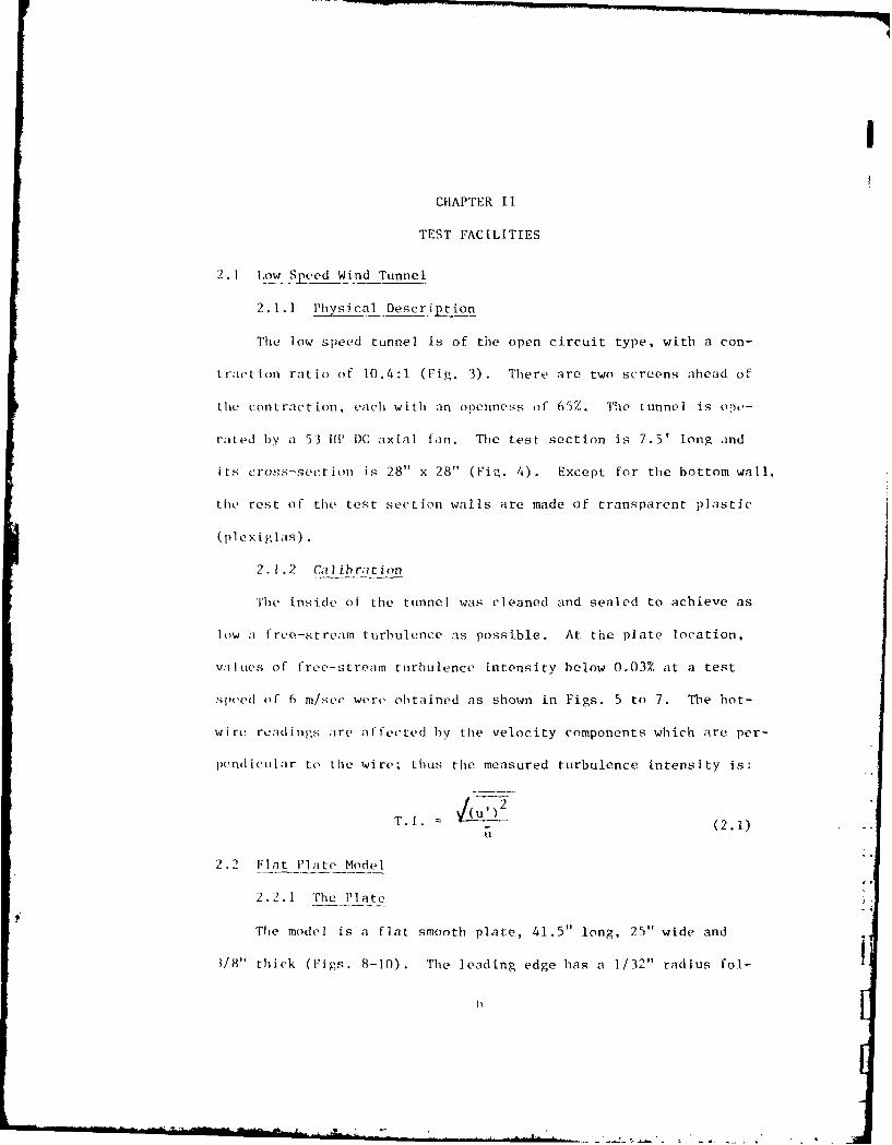
2.1 Low Speed Wind Tunnel

2.1.1 Physical Descript ion

The low speed tunnel is of the open circuit type, with a con-

trart ion ratio of 10.4:1 (Fig. 3). There are two screens ahead of

the contraction, each with an openness of 65%. The tunnel is one-

rated by a 53 IP )C axial fan. The test section is 7.5' long and

its cross-section is 28" x 28" (Fig. 4). Except for the bottom wall,

the rest of the test section walls are made of transparent plastic

(plexiglas) .

2.1.2 Calibrat ion

The inside of the tunnel was cleaned and sealed to achieve as

low a free-stream turbulence as possible. At the plate location,

v.a lues of free-stream turbulence intensity below 0.03% at a test

speed of 6 m/see were obtained as shown in Figs. 5 to 7. The hot-

wire readings are affected by the velocity components which are per-

pendicular to the wire; thus the measured turbulence intensity is:

T.. -(2.1)

u

2.2 Flat Plate Model

2.2.1 The Plate

The model is a flat smooth plate, 41.5" long, 25" wide and

1/8" thick (Figs. 8-10). The leading edge has a 1/32" radius fol-

I)l

7

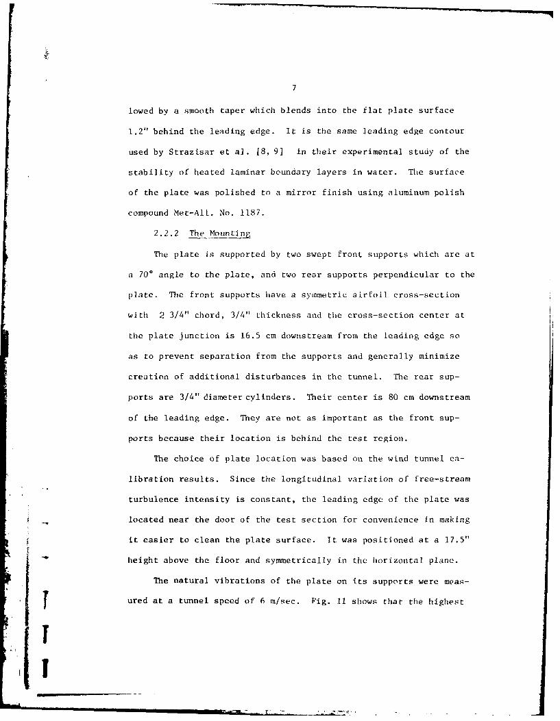
lowed by a smooth taper which blends into the flat plate surface

1.2" behind the leading edge. It is the same leading edge contour

used by Strazisar et al. [8, 9] in their experimental study of the

stability of heated laminar boundary layers in water. The surface

of the plate was polished to a mirror finish using aluminum polish

compound Met-All. No. 1187.

2.2.2 The Mounting

The plate is supported by two swept front supports which are at

a 700 angle to the plate, and two rear supports perpendicular to the

plate. The front supports have a symmetric airfoil cross-section

with 2 3/4" chord, 3/4" thickness and the cross-section center at

the plate junction is 16.5 cm downstream from the leading edge so

as to prevent separation from the supports and generally minimize

creation of additional disturbances in the tunnel. The rear sup-

ports are 3/4" diameter cylinders. Their center is 80 cm downstream

of the leading edge. They are not as important as the front sup-

ports because their location is behind the test region.

The choice of plate location was based on the wind tunnel ca-

libration results. Since the longitudinal variation of free-stream

turbulence intensity is constant, the leading edge of the plate was

located near the door of the test section for convenience in making

it easier to clean the plate surface. It was positioned at a 17.5"

height above the floor and symmetrically in the horizontal plane.

ured at a tunnel speed of 6 m/sec. Fig. 11 shows that the highesturThe natural vibrations of the plate on its supports were ineas-

*1

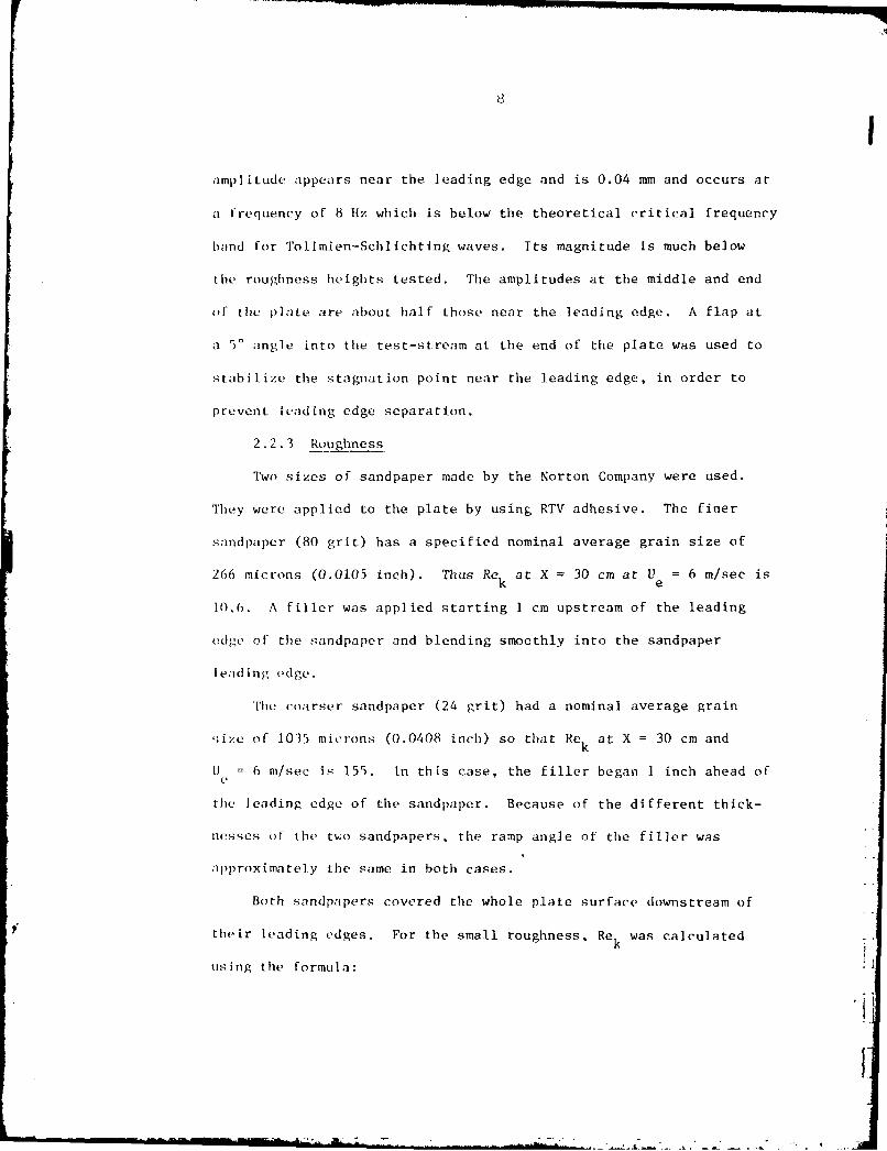
amplitude appears near the leading edge and is 0.04 mm and occurs at

a frequency of 8 liz which is below the theoretical critical frequency

band for Tollmien-Schlichting waves. Its magnitude is much below

the roughness heights tested. The amplitudes at the middle and end

of the plate are about half those near the leading edge. A flap at

a 50 angle into the test-stream at the end of the plate was used to

stabilize the stagnation point near the leading edge, in order to

prevent leading edge separation.

2.2.3 Roughness

Two sizes of sandpaper made by the Norton Company were used.

They were applied to the plate by using RTV adhesive. The finer

sandpaper (80 grit) has a specified nominal average grain size of

266 microns (0.0105 inch). Thus Rek at X = 30 cm at Ue = 6 m/sec is

10.6. A filler was applied starting 1 cm upstream of the leading

edge of the sandpaper and blending smoothly into the sandpaper

leading edge.

['he coarser sandpaper (24 grit) had a nominal average grain

;ize of 1035 microns (0.0408 inch) so that Rek at X = 30 cm and

U = 6 m/sec is 155. In this case, the filler began 1 inch ahead ofe

the leading edge of the sandpaper. Because of the different thick-

nesses of the two sandpapers, the ramp angle of the filler was

approximately the same in both cases.

Both sandpapers covered the whole plate surface downstream of

their leading edges. For the small roughness, Rek was calculated

using the formula: .

i-

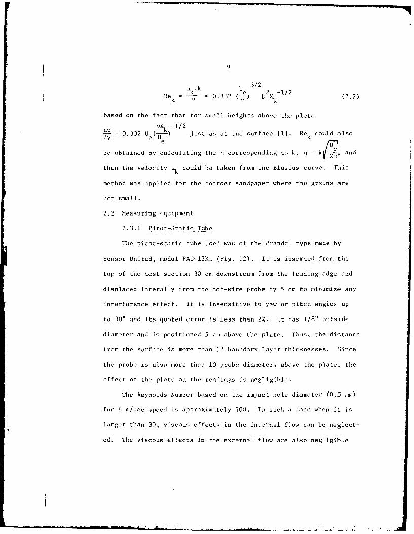
9

u~k U3/2Ukk e k2X-1/2(2)

Rek = k - 0.332 (-7) k X(2.2)

based on the fact that for small heights above the plate

vXk -1/2du = 0.332 U e k(U-- just as at the surface [1]. Rek could alsodyeUk

be obtained by calculating the n corresponding to k, n = k / S andX\v

then the velocity uk could be taken from the Blasius curve. This

method was applied for the coarser sandpaper where the grains are

not small.

2.3 Measuring Equipment

2.3.1 Pitot-Static Tube

The pitot-static tube used was of the Prandtl type made by

Sensor United, model PAC-12KL (Fig. 12). It is inserted from the

top of the test section 30 cm downstream from the leading edge and

displaced laterally from the hot-wire probe by 5 cm to minimize any

interference effect. It is insensitive to yaw or pitch angles up

to 300 and its quoted error is less than 2%. It has 1/8" outside

diameter and is positioned 5 cm above the plate. Thus, the distance

from the surface is more than 12 boundary layer thicknesses. Since

the probe is also more than 10 probe diameters above the plate, the

effect of the plate on the readings is negligible.

The Reynolds Number based on the impact hole diameter (0.5 nm)

for 6 m/sec speed is approximately 100. In such a case when it is

larger than 30, viscous effects in the internal flow can be neglect-

ed. The viscous effects in the external flow are also negligible

10

when the Reynolds number based on the probe radius is larger than

100, which is the case here.

For T.I. around 0.03% and dynamic pressures of about 0.1 in.

li2(0 ,he fluctuation velocity component dynamic pressure, 1p(u)

-9corresponds approximately to 9 x 10 in.H2 0. This is negligible

relative to 0.1 in.1 20. Thus, the pitot tube reading is insensitive

to sinai I I t urbu I ence.

The time constant for the pitot probe is approximately five

seconds.

The probe is connected to a Meriam i,tanoirieter wh-ich ir A-1l

ti, ma.sure 0.001 in. f20 (Fig. 15).

2. 1.2 Hot Wire

The shape of the hot-wire probe was designed appropriately for

boundary layer measurements (Fig. 13). It consists of 1/4" stainless

st,.el tubing in which electrical wires run through, that are con-

netcteLd to the copper prongs. The prongs are insulated one from the

other by 5 minute epoxy. The tips of the prongs are connected by

Wol laston wire (907 platinum, 10% rhodium) 8 mm long.

"The length of the control portion which is the sensor varies

depending on the etching procedure during its preparation and is

.ipproximately 0.8 mm long. Beneath the joining of the prongs there

is a protruding support made of 5 minute epoxy. From cathetometer

m&k;,tirements supported by mean velocity profile results, the wire

is 0.2 mm above the support bottom.

The principle of the hot-wire and the factors affecting its

operration are described briefly as follows:

il

The wire is heated by a constant current. It is cooled by the

flow causing the temperature to drop and,consequently, the electric

resistance to diminish. It is cooled primarily by forced convection

and heat conduction. Total amount of heat transferred depends on:

I) The flow velocity

2) The difference in temperature between the wire andthe fluid

.3) The physical properties of the fluid

4) The dimensions and physical properties of the wire

The last three are known and thus the flow velocity can be

measured.

The hot-wire anemometer is still a prime instrument for tur-

bulence measurements. Its principal advantage is the separation of

the mean velocity from the fluctuating components and the ability to

measure them separately at the same time. The other main advantage

is in its being thin. The Reynolds number based on wire diameter

is !.54 for a speed of 6 m/sec. This is below 3, which is the limit

for smooth flow around the wire without separation even with heating,

because Reynolds number dec toases with temperature 111 (Pig. 14). The

thermal inertia of the thin wire is very small and thus the response

for frequencies of interest in this experiment (tip to 5 KHz) i.-

practically instantaneous. It catches less dirt than a thick sensor

and altogether it is sufficiently strong and rigid to sustain

vibrations and stresses caused by turbulence. The measured velocity

is in good agreement with the flow velocity as measured using the

-I- .

12

pitot-static tube for turbulence intensity smal ler than 10%.

The joining of the prongs is 32,000 wire diameters behind the

wire and thus there is no real influence of the prongs on the flow

around the sensor portion of the wire.

There are two problems with the hot wire. The first is

drifting and the second is contamination. Both can be treated prop-

k-rly is will be explained in the next chapter. More about hot wires

cn, be found in ref. [11 1.

The hot-wire anemometer set is a Shapiro and Edwards model 50

(Fig. 15). It includes an amplifier, a resistance bridge, a poten-

ti,imetecr, ; mean square output meter and a square wave generator.

i'lh. potentiometer allows measurement of wire currents up to 10 - 5 amp.

and so enables accurate velocity measurements. A compensation cir-

(nit is available but is needed only for frequencies above 5KHz and

wa.s not utilized in this experiment.

The preparation of the hot-wire sensor is as follows: First,

the wire is soldered to the prongs and then the probe is attached to

ai poitioner. The wire is brought into contact with a small drop of

70' concentrtLd ritric ;1cid (Pigs. 16-17). An electrolyzing cur-

rent is supplied by a 1 1/2 volt Eveready battery for about one Nminute. The length of the uncovered (etched) center portion of the

wire is a function of the drop size, and is of the order of 0.8 mm.

This prtion whiich is the sensor has a diameter of 0.00015 in. jThe wire is thewn checked using a microscope which magnifies

60 times. It is important to have a straight and clean wire.

.... .... .[

13

The soldering of the wire to the prongs with a soft solder had9to be done quickly in order not to create excessive heat in the wire

and thus avoid any elongation. If overheated, the uncovered portion

of the wire could not sustain as much stress as the rest of rhe wire,

and at the end of the etching process would become deformed.

The other factor which affects wire shape is the surface tension

of the drop. To avoid any adverse effect, the wire has to be taken

out of the drop very carefully.

2.3.3 Traverse Mechanism

The traverse mechanism (Fig. 19) was designed to give accurate

vertical readings of the probe position. It has a metric Mitutoyo

micrometer which can be moved longitudinally with the help of a

motor. There is an error of -0.2 mm in longitudinal positioning.

The micrometer enables vertical precision to 10.01 mm and so this is

the accuracy of the hot-wire probe position because it is attached

to the micrometer. The height can be read on the micrometer scale

and readjusted to zero each time the hot wire is brought to the

plate surface. The precision of lateral positioning is not as impor-

tant as the vertical one and there is an estimated error in lateral

position of at most 0.5 mm.

The traverse mechanism is outside thte top of the test section

and the hot-wire probe goes through and moves in the slot made in

the top wall. This location of the mechanism was chosen because it

allows the probe to have a simple shape, has a shorter shaft than

a probe from the side wall and does not vibrate at the test speed.

I

14

It also creates less disturbance than a probe from the side wall.

The slot was placed above the middle of the plate where the

turbulence intensity is smallest.

2.3.4 Spectrum Analyzer

A Unigon Model 4512 spectrum analyzer was used to measure

spectra. It has an averaging capability for a chosen time interval.

lh, bandwidth and the amplitude scale could be adjusted. A Polaroid

camera attached to the screen enabled pictures of the spectrum

to be taken.

9

4I

I

CHAPTER ITI

EXPERIMENTAL PROCEDURE

3.1 Calibration

Calibration of the hot wire was performed with every run

because the cold wire resistance was changing due to heat, dust and

natural deterioration. To eliminate drifting, it was necessary to

allow two hours for the system to warm up before using the hot wire.

The contamination problem was solved by changing the wire every few

weeks.

Calibration was always performed with the wire at 5 cm above

the plate, and 30 cm downstream of the leading edge. The cold wir2

resistance R was measured. The overheat ratio of 1.3 was ad-0

juisted by setting the wire resistance R to a value of 1.3 R 0W O

The wind tunnel speed was increased gradually and each time the

wire current and the manometer readings were taken. In such a

manner, the calibration curve for the velocity as a function of the

wire current was obtained and plotted (Fig. 19). It was almost a

straight line as it should be according to King's law [ill:

2 a + b (3.1)

After the calibration, the pitot tube was pulled out.

3.2 Smooth Plate

3.2.1 Adjustment of Zero Pressure Gradient

The outer flow velocity was measured along the plate using the

15

16

hot wire because it is more accurate than a pitot tube for such

small pressure differences as in this case. At each place where the

hot wire was positioned, the slot was sealed off with masking tape.

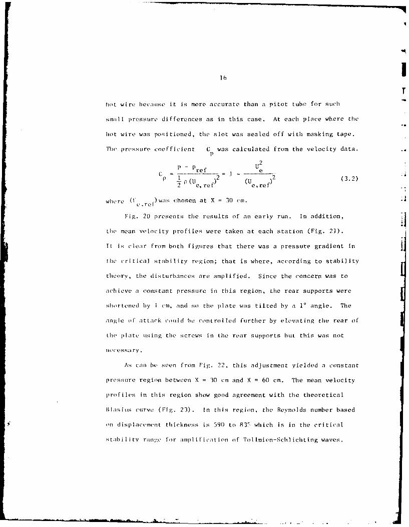
The pressure coefficient C was calculated from the velocity data.

P - ref I eC= 1 )2f (3.2)

p (U 2 (U2 e,refre

where (le,rcl) wais chosen at X = 30 cm.

Fig. 20 presents the results of an early run. In addition,

the mean velocity profiles were taken at each station (Fig. 21).

It is clear from both figures that there was a pressure gradient in

tile critical stability region; that is where, according to stability

theory, the disturbances are amplified. Since the concern was to

achieve a constant pressure in this region, the rear supports were

shortened by 1 cm, and so the plate was tilted by a I' angle. The

angle of attack could he controlled further by elevating the rear of

the plate using the screws in the rear supports but this was not

lcessa ry .

As can be seen from Fig. 22, this adjustment yielded a constant

pressure region between X = 30 cm and X = 60 cm. The mean velocity

profiles in this region show good agreement with the theoretical

lilisius curve (Fig. 23). In this region, the Reynolds number based

on displacement thickness is 590 to 83Y which is in the critical

stability range for amplification of Tollmien-Schlichting waves.

17

Thus, the region between X = 30 cm and X = 60 cm was chosen as the

test region.

3.2.2 Measurement of Mean and Fluctuating Information

The mean and the fluctuating information was taken at the same

time. For the smooth plate, the probe was lowered until the support

touched the plate. This was repeated several times and the micro-

meter readings were taken. They were always within -0.03 mm of a

mean value and thus could be considered accurate enough. At this

position, the wire was approximately 0.2 mm from the surface. This

was the closest position from the plate and there the first readings

were taken. Measurements were repeated at vertical intervals of

0.5 mm until there was no current change, indicating the outer flow

regime.

At each point, the current, the series resistance and the

average wire voltage (e')2 were measured. This enabled calculation

and extraction of the information of interest. The mean velocity

was taken from the calibration curve (Fig. 19) for the corresponding

current. The fluctuation rms velocity component was calculated as

follows [11]:I(e,)2

u)2 (e- (3.3)

R I aEZwhere S = is a hot-wire sensitivity

R = 1.3 R - the wire resistance at overheatw 0

I - the wire currentw

18

a =(R W-R )/R 0.3

I = (-: )/(l+2,) where F = R /(R + R ) andW S W

j- the series resistance

7 1/(1+ / /vj) where 51 is the corresponding velocity0 0

for a zero current and extrapolated from the cali-

brat ion curve

u the mean velocitv

The volt.:', -/,,'was measured by taking approximately 50

readings at 5 second intervals.

By calculating (u_1)2 U , it was easy to get the dis-r ins

turbance energy and the free-stream turbulence intensity

h or the local intensity (U') 2 /u.

3.I Roiugh Plate

3. t.l Additional Adjustments

The finer sandpaper was at first positioned to begin at 3 cm

dwnstream of the leading edge. The Rek and k/(S* at this location

are 33 and 0.56 respectively. The boundary layer was apparently

tripped by the leading edge of the sandpaper and the flow at the

first measuring station,X = 30 cm,was already turbulent. The paper

was then cut back to 6.5 cm downstream of the leading edge of the

plate. The corresponding Rek and k/g* were 23 and 0.38 respecti-

vely. Here the flow was laminar at the first station and for this

location of the leading edge of the sandpaper, the measurements

Were taken.

The coarser sandpaper began initially at 6.5 cm from the lead-

19

ing edge of the plate but again the boundary layer was tripped.

The corresponding Rek and k/6* were 314 and 1.48 respectively.

The flow was turbulent even at X = 20 cm. When the paper was cut

back to 18.3 cm, the flow at the first station was laminar. At

X = 18.3 cm, Rek = 192 and k/6* = 0.88. This was the location of

the leading edge of the coarser sandpaper for the measurements

presented herein.

3.3.2 Measurements Taken with Each of the Two Sandpapers

The measurements and the procedure for the finer sandpaper was

similar to those for the smooth plate. For measurements with

coarser sandpaper, precautions had to be taken to prevent wire

damage.

A glass plate of 1.4 mm thickness was placed on the surface

under the probe and the probe was lowered until the support touched

the glass plate. The micrometer reading was taken. The probe was

raised and the glass plate removed. The probe was lowered again by

1.4 mm beneath the reading. At all stations, it was possible to

lower the probe an additional 0.5 mm without damaging the wire. The

probe location was illuminated, and it was always possible to see a

gap between the wire and the grit. This was checked many times. This

is possible because of the non-uniform distribution of the grains

in the sandpaper matrix and also because of some grains which were

positioned above the average. If the plate rested on those higher

grains, then the wire could be lowered beneath their height. We

could assume that there were enough grains of such size to allow

I

20

this to occur. Thus, the first reading for the roughest sandpaper

was taken with the wire at 0.3 mm below the highest grains in the

near vicinity where the measurements were taken.

fn addition to the measurements as taken earlier, special

data were taken for the coarser sandpaper. Here the information

was taken also at X = 20 cm. The hot-wire probe was positioned at

the peak energy location. The amplitudes were measured from Pola-

roid pictures of the analyzer output and the amplification rates

were calculated from:

0 1 dA (3.4)S A dX

The amplitude gradient was measured from the amplitude curves.

Data were also taken using the filters on the hot-wire anemo-

meter panel. At the peak energy location for each station, the

energy was measured for different frequency bands. The filters were

1-10, 10-100, 100-5000 Hz.

i:i

, , - w t, . - • _ -,

CHAPTER IV

RESULTS AND DISCUSSION

4.1 Smooth Plate

To provide a reference for the later measurements with surface

rou .hness, a set of mean and fluctuating measurements was taken

on the smooth aluminum plate. The mean velocity profiles at X = 30,

40, 50 and 60 cm downstream of the leading edge are shown in

'igs. 24 (a-d). Two data -sets taken at different times are shown.

The Blas iu:s curve taken from Sch ichting [121 is plotted for com-

parison on each of the fipares. The points agree with the Blasius

curve within the experimental error. The profiles corroborate

the earlier indication from surface pressure measurements that the

region 30 • x . 60 cm is -i constant pressure region.

(ne set of test results for the fluctuation energy nondimension-

;ilized with respect to 2 versus dimensional boundary layer coordi-C

nate v and nondimensional ri is presented in Figs. 25a and 25b

respectively.

The free-stream turhulence and the wind tunnel fan rotation

affect the magnitude of the disturbance energy, but the shape and

order of magnitude of the curves remains consistent. Even though

the data points are not always on the curve lines, the deviation is

within the experimental error and the curve lines are definitely

21wIhl h xermna n h

22

characteristic of the phenomena taking place according to other

test results taken in tile present investigation. The shape is si-

milzar to that obtained in other experimental studies for a smooth

plate, for example that of Strazisar et al. [8,91.

The integrals under the curves and the peak values are increas-

ing consistently and gradually in the downstream direction. The

energy content is distributed over the whole boundary layer but is

concentrated mainly in the middle. It is almost symmetrically dis-

tributed. The peak moves away from the wall but remains at

ri 2.3 or y /4 0.43 and Y max/6* 1.37. The peak energy is

increasing approximately linearly with distance downstream.

The local disturbance intensity which is with respect to the lo-

I:,l velocity 4s plotted in Fig. 26. It is seen to decrease near the

wall with downstream distance. The energy integrals and peak values

are increasing but very little. Both the energy and the local

iiitensitv are increasing in the vicinity of the edge of the boundary

laver, thus indicating that tile response to free-stream disturbances

is not confined to the interior of the boundary layer. The turbu-

lence intensitv at the outer edge is seen to increase about 0.02%

with every 10 cm downstream from the leading edge.

The reasons for showing both energy and local turbulence inten-

sity will becomc apparent later in the cases with roughness.

4.2 Distributed Roughness of Re k (X = 30 cm) = 10.6

Similar measurements were taken for this roughness as for the

23

smooth surface. The mean velocity profiles at X = 30, 40, 50 and

60 cm downstream of the leading edge are shown in Figs. 27 (a-d).

Just as for the smooth case, a number of data sets were taken and

the Blasius curve is plotted for comparison on each of the figures.

The zero reference height, as for the smooth wall case, was assumed

to be 0.2 mm beneath the hot-wire when the probe support touched

the surface. With this choice of ri = 0 (y = 0), the Blasius curve

fits the data points within the experimental error.

One set of test results for the energy is presentcd in

Figs. 28 a,b. The shape and order of magnitude of the curves for this

run remains consistent for the results of other tests taken in this

investigation but not shown. The energy has the same shape and the

same gradual increase as for the smooth case. It is again mostly

concentrated at the center of the boundary layer and the peak

remains at rn 2.3 as for the smooth surface.

We can see already slightly more curvature near the wall than

in the smooth wall case (Fig. 25b) as the flow proceeds in the

downstream direction. The energy at the outer edge of the boundary

laVer is also slightly larger than for the smooth plate. Within the

boundary layer the energy levels are slightly smaller than for the

smooth surface perhaps because the speed was lower by 0.2 m/sec and

possibly because the flow was less turbulent initially, thus affecting

the initial energy levels. Although the energy peak at X 30 cm is

smaller than for the smooth wall case, the energy growth - the

raitio of energy at the last station to that at the first station -

I

I!

24

is 107 larger than before and that.perhaps, is an indication of a

slight roughness effect.

A more pronounced indication of the roughness effect is shown

by the local turbulence intensity distribution presented in Fig. 29.

Even though the energy was smaller, the intensities were larger than

those for the smooth wall (Fig. 26) in the vicinity of the wall.

The intensities of the peaks close to the wall are increasing with

downstream distance in contrast to the results for the smooth

surface.

In summnr v , this small roughness (beginning from Rek = 22.8

and k/M* = 0.38 at X = 6.5 cm) has only a very small effect. 7t

doesn't perturb the flow to the nonlinear regime and both the mean

velocity and the disturbance energy profiles resemble those of

laminar flow on a smooth plate. Although the overall effects are

small, we could detect changes in the local turbulence intensity

distribttions, particularly in the vicinity of the wall.

,4. 1listrihuted Roughness of Rek (X = 30 cm) = 155

4.3.1 M ean and Fluctuoation Measurements

A set of mean velocity profile, is shown in Figs. 30 (a - d).

In thiis case the roughness is large enough so that the effective

zero velocity location for the boundary layer could not be deter--

mined a priori. The data point closest to the wall was 0.3 mm

below the top (f the largest grains. This point was chosen as the

r' erence location for the rest of the data taken. The nominal

25

grit size is known and thus the distance of the reference location

point from the nominal bottom of the grains is al.o known. By

fitting a curve through the data points, the extrapolated zero velo-

city point can be located. For the first two stations (X = 30 cm,

X = 40 cm), a Blasius curve could reasonably be put through the

data points and the extrapolated zero velocity locations were at

approximately tie same distance from the nominal bottom of the grit

(0.2 mm). An attempt to fit the data points with a similarity pro-

file for = -0.1 was unsuccessful. ihese two measured profiles are

much closer to the Blasius curve and compare very well with the

measured data on the smooth plate once an adjustment is made for

the extrapolated zero.

Curves through the mean velocity data points for the two down-

stream stations (X = 50 cm, X = 60 cm) are shown in Figs. 30c and

30d. The extrapolated zero velocity location is chosen to be the

same as in Figs. 30a and 30h. Blasius curves are drawn for compa-

rison. At X = 50 cm the mean velocity profile has changed signifi-

cantlv from that at X = 40 cm. At X = 60 cm there is the beginning

of the emergence of a turbulent profile shape.

If there are inflection points near the wall in Figs. 30a and

30b, it is practically impossible to detect them considering the

experimental error. It is also very difficult to do a detailed

search in the vicinity of the grit because of prospective wire

damage and probe interference effects.

i

26

Fluctuation data for two separate tests taken a week apart are

shown in Figs. 31a, b. The first test results are indicated by 1

and the second by I. The first test corresponds to the mean velo-

city results shown earlier (Fig. 30).* The n = 0 locations used in

these figures for each station were taken from the extrapolated zero

velocity points of the mean velocity profiles. The shape of the

energy distributions is not smooth but somewhat oscillatory. Both

tests show more thian one local peak and the number increases with

the distance downstream. The first two stations display more or less

their previous shape. Their peaks are in the vicinity of ri 2.3

and only the second test deviates from this slightly at the second

stat ion. The downstream profiles here are much fuller than for the

smooth pl;.,te or the finer roughness and there is significant

increase in energy content near the wall.

For the finer roughness the only clear indication of a rough-

nc-s- effect was through the changes in the turbulence intensity dis-

trihutions. Here we see a large effect on the energy distributions

as wol 1. The peaks are moving closer to the wall and most of the

energy content is concentrated in the rn < 4 region for the first

three stations. Farther downstream there is also significant

increase in energy content at the outer edge of the boundary layer.

* Mean velocity profiles for test 11 (4/21/80) were measured atX = "30 cm and X = 40 cm, they are very close to the profiles ofFigures 30a and 30h. The profiles at X = 50 cm and X - 60 cm differs i ghtlv from those of Figures 30c and 3ld in a manner consistentwith the different progressions to trans ition on those two days.

I'1

5 27

In between X 40 cm and X = 50 cm where a velocity profile change

takes place, the energy increases by an order of magnitude. Figs.

32a,b present the local turbulence intensity for these two tests

respectively, again using the extrapolated zero from Test I. The

local intensity rises to more than 15% between X=40cm and X= 50 cm

emphasizing that the disturbances are in the non-linear regime.

In Test I, there is not much overall energy change between the

last two stations but there is a noticeable buildup in the outer

portion of the boundary layer. Accompanying this is a definite

change in the mean velocity profile (Figs. 30c,d) and an increase

in the boundary layer thickness even though it is not yet a fully

turbulent flow.

Test II shows a flow that seems less disturbed initially. Less

of an increase in energy occurs between X = 40 cm and X = 50 cm.

As a consequence, there is still an increase in energy bet,.etn the

the last two stations. Only the last station indicates a signifi-

cant energy increase in the outer portion of the boundary layer.

'[e mean velocity profiles which are not presented here, again

indicate a Blasius profile for the first two stations and a very

slight change relative to Test f at the third station. The inten-

sity peak at the last station reaches the same magnitude as at the

last two stations of Test I.

The intensity shape is bumpy. However, the main peaks are approach-

ing the w:4ll ,consistent with the observation for the Re k= 10.6 case.

The peaks are within the region n - 0.5. At the measurenlent point

closest to the wall, the total amplitude ratio relative to free-

II

28 1stream turbulence level (assumed to be 0.02%) for both experiments

7.3is already about 1500 which is e . The boundary layer at this

point is however not yet fully turbulent. Maybe the ratio is larger

closer to the wall but it was impossible to measure any closer.

The consistency of the peak intensity development shown by

Igs. 32a, b with that of the finer roughness indicates that the

extrapolated zero point is reasonablv chosen. The development of

the energy and the intensity indicate that the fully turbulent

regime is not yet reached.

An attempt to isolate a roughness effect for Test II by

Subtracting Fig. 26 (the smooth plate intensity) from Fig. 32b (the

rough plate intensity) is presented in Fig. 33. The curves are

essentially the same as in Fig. 32b indicating that the overwhelming

contribut ions to the data in Fig. 32b are due to the roughness.

Fig. "34 shows the variations of the peak local intensity and

the square root of the peak nondimensional energy with Re . Thesex

restlts are consistent with what was said earlier: (a) the intensity

is more sensitive than the energy and thus a better indication of

tlik, degree to which the flow is disturbed; (b) the flow in Test I

I; more d i ;I ri.bcd.

In summary, the intensity magnitudes for both experiments are

,ihove 15% at the third station (X = 50 cm) and thus are clearly non-

linear. The intensity for the second station is 4.5 - 87 and thus

significant too and probably non-linear. The main conclusion is

that the disturbances grow to non-linear amplitudes before detect-

able velocity profiles are observed.

-. *

29

4.3.2 The Spvctrum

In addition to mean and fluctuation measurements, one set

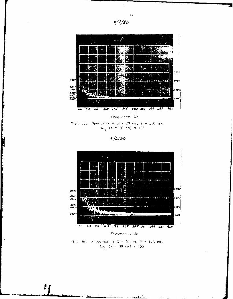
of tests was made using the Unigon spectrum analyzer. Figs. 35 - 39

show the spectra taken at X = 20, 30, 40. 50 and 60 cm with the

coarsest paper and U 6 m/see. For X = 20 cm to X= 40 cmC

(Figs. 35, 36, 37) gain settings were inadequate to get data .ibove

20 Hz from those pictures. It was possible to read the amplitude

above 20 liz for the last two stations but the accuracy is doubt-

ful , and since the amplitude slope is very sensitive to any small

amplitude change, the calculated -. values are doubtful too.

Nevertheless it is possible to extract some important information

from this test.

AmpI i tude distribution.s for f requencies up to 17.2 llz are shown

in Fig. 40. They have a shape resembl ing what is obtained in linear

stabi Ii tv studies. Fig. 41 presents the calculated amplification

rates - . Ft.r 17.2 11z amp lif ication occurs it Re 550. As the

Re O increases, su-cessivelv lower frequencies become amplified but

their maximum ,Unpl ification rate is diminishing. The highest ampli-

ication rate for 17.2 Hiz is located at Re = 650. Lower frequen-

ciese show peak (i it succesSiV v lirger vai ,nes of Re,. These

p,'..,; occur i n the non-[Ill, iLar region of the flow as identified from

energy ;nd iteilsitv distribut ions. Fig. 42 shows again that as

Re , incre'es, the lower 1requn nlic.; become important. A plot of

ma vr;ums Re (l"y1. '3) indicatos 1hat highor freqienci!,s (;boveIMa x

I

I

30

17.2 Hz) may be important below Re = 650. Note that the Tollmien-

Schlichting band at Re,* 650 is between 45 - 85 Hz. In fact if

we extrapolate the trends of Fig. 41 to higher frequencies, it would

suggest the higher frequencies become more important close to the

leading edge.

Amplification rates -ri. for the frequencies up to 130 Hz at

IIX = 50 cm are shown in Fig. 44. Similar behavior of a. i i, found at

X = 60 cm. Amplification is shown at all frequencies. There does

not seem to be anything special about the Tollmien-Schlichting

band. Again, at X = 50 cm, the disturbances are non-linear.

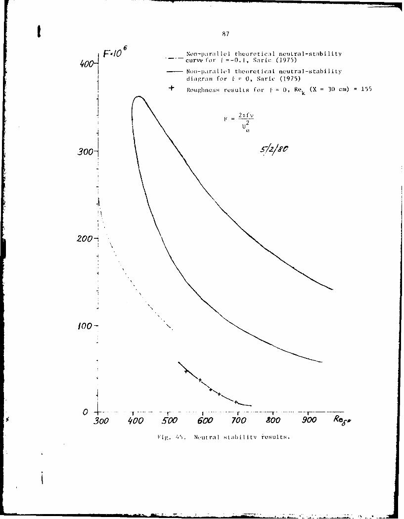
The experimental "neutral curve" for frequencies up to 17.2 Hz

is below the neutral curve for the linear stability of non-parallel

flat plate flow as calculated by Saric [13] (Fig. 45). It is also

below the neutral curve for the linear stability of non-parallel

Valkner-Skan flow corresponding to L = -0.1. This corroborates the

earlier indication that disturbance growth was governed by non-

linear growth effects rather than by linear instability of an in-

flectional mean velocity profile which hasn't been detected in any

case.

From the trend of the curve we can definitely say that there is

earlier amplification and very likely earlier transition than for

tLh smooth sur face. While the linear theory for a smooth plate

Iredicts t. for Re, above 684, here it i larger much below thisma X

number. The order of magnitude of (a. ) is also totally1 cr maxtoal

(Ii F fe rent

f 31i

The maximum value of ( ) for non-parallel smooth flatRe86

plate flow is approximately 9.55 x 10-6 and occurs at Re, = 795 [9].

For the same Re * the present data for the rough case shows it equal

-52.67 x 10 and the value of i is even higher for lower Re,. This

means faster transition. Considering the state of the boundary

layer at X = 60 cm (Re6 , = 835), transition might be completed at

ReX 350,000 which is very low compared to the value of 3 x 106

that might be expected on a smooth plate for the low free-stream

turbulence intensity of the tunnel.

Frequencies corresponding to roughness wavelengths are of order

Uk 0k= ()w " In the present experiment such frequencies would be in

the range of 1.5 to 3 Kltz. No growth was observed in these frequency

bands.

4.3.3 Filtering

Another experiment was performed using the built in filters on

the hot-wire anemometer set at the peak energy location at X = 30,

40, 50 and 60 cm downstream from the leading edge. The filters were

1-10, 10-I0, 100-5000 Hz. Fig. 46 shows the energy results for

these frequencv levels.

There is a shift in energy to higher frequencies. Most of the

energy in the non-linear regime is concentrated in the 100-5000 Hz

band. This didn't show up from thi spectrum because even though

the amplitude in the high frequency range is small, its integral is

significant and very sensitive to a small amplitude increase, since

II

32

lie band width of the 100-5000 liz band is so large. Major high

frequency content is probably in the 100-200 liz band. The mechanism

is driven by frequencies up to about 140 Hz as indicated by the

Spectra (Figs. 38, 39), but the energy is dissipated into higher

frequent ies.

4.4 Leading Edge of the Distributed Roughness

As described in the preceding chapter for both roughness sizes,

the leading edge of the sandpaper had to be cut back in order that

the boundary layer not be tripped by the leading edge of the sand-

paper. Such tripping did occur before cutting back the sandpaper,

despite the use of a filler to avoid a step at the leading edge of

tLhe sandpaper.

The finer roughness sandpaper was cut from X = 3 cm with the

corresponding Rek = 33 and k/6* = 0.56,to X = 6.5 cm downstream from

the leading edge and the corresponding Rek 22.8 and k/6* = 0.38.

Before the cutting back the sandpaper, the flow was turbulent over

the whole test region and after cutting it back it was laminar.

"The coarser roughness paper was cut back from X = 6 cm with the

corresponding Rek = 314 and k/6* = 1.48,to X = 18.3 cm with corres-

ponding Rek = 198 and k/6* - 0.88. Before cutting the sandpaper back,

transition was detected already at X =20 cm and turbulent flow oc-

curred in the whole test region. After cutting back the 'andpaper,

laminar mean profiles were obtained at least to X = 40 cm (Fig. 30).

3 *3

Even though Rek was equal to 198 at the leading edge of the

coarser sandpaper and only 33 at the leading edge of the finer sand-

paper and the filler ramp angle was approximately the same in both

cases. the latter tripped the boundary layer while the former did

not. Thus Rek is not the only parameter affecting the flow. The

same can probably be said about k/t)*. Thus, the response of the

f low to the Iending edge of i rougness region cannot be simply

described in terms of these two parameters. The filler strip

geometry and the smoothness achieved are important factors in

influencing the flow.

CHAPTER V

SUMMARY AND CONCLUSIONS

A preliminary experimental study has been completed of the dis-

turbances in a laminar boundary layer due to distributed surface

roughness. Tests were conducted on a smooth plate and with two dif-

ferent grades of sandpaper covering.

Over the portion of the smooth plate displaying zero pressure/

gradient (30 cm < x < 60 cm), the mean flow velocity profiles agree

with the Blasius profile within the experimental error. The u'

rms

distributions display a peak at q z 2.3 that increases slightly with

distance downstream reaching a level of 0D07 U at X = 60 cm.e

For distributed roughness having Rek 10, the results are quite

comparable to those for the smooth plate. The mean flow velocity

profiles agree with the Blasius curve within the experimental error

and the u' distributions are closely comparable in level andrms

distribution to those for the smooth plate. There is however indi-

cation of a slight increase in local intensity in the very near vici-

nity of the wall. It is well to point out that although the dimen-

sionless turbulent energy (u' /U )2 and the local turbulent inten-rms e

sity (u' rms/u) involve the same fluctuation amplitudes, the local

turbulent intensity is a much more sensitive indicator of effects of

roughness.

34

i i i 'I i I I ' - -_

35

For distributed roughness with Rek - 150, the picture is dif-

ferent. At X = 30 cm and at X = 40 cm, the mean velocity profile is

best fit by a Blasius profile whose effective origin is somewhere

within the roughness height. Beyond X = 40 cm the mean profile

seems to progress toward a turbulent profile. Up to X = 40 cm, the

u' still peaks at n z 2.3 but the local intensity is now of therms

order of 5%. Beyond X = 40 cm there is a large increase in the u'rms

levels and an increase in the number of peaks. Very large local

intensities are obtained in the near vicinity of the wall (n < 0.5)

but there is also noticeable buildup over the entire boundary layer

to the outer edge. A study of disturbance spectra for this case

shows largest amplitudes and amplifications at frequencies well

below the Blasius neutral curve. The maximum amplification rates

are about th'ree times as large as those for Tollmien-Schlichting

instability over a smooth plate. Transition occurs at

Re x _ 350.000 which is much below the value of 3 x 106 or so that

might be expected for a smooth surface at the turbulence level of

the tunnel.

To conclude, one observes that disturbances can grow to non-

linear magnitudes before velocity profile changes are observed.

The indicated importance of frequencies below those of the Blasius

neutral curve was not expected and requires more careful examination.

REFERENCES

1. Dryden, H.L.: Review of Published Data on the Effects of Rough-ness on Transition from Laminar to Turbulent Flow, .1. Aero-nautical Sci., Vol. 20, No. 7, pp. 471-482, July 1953.

2. Smith, A.M.O. and Clutter, D.W.: The Smallest Height of Rough-ness Capable of Affecting Boundary-Layer Transition.J. Aerospace Sci., Vol. 26, No. 4, pp. 229-245,256, April1959.

3. Klebanoff, P.S. and Tidstrom, K.D.: Mechanism by Which a Two-Dimensional Roughness Element Induces Boundary Layer Tran-sition. Physics of Fluids, Vol. 15, No. 7, pp. 1173-1188,July 1972.

4. Singh, K. and Lumley, J.L.: Effect of Roughness on the VelocityProfile of a Laminar Boundary-Layer, Appl. Sci. Res.. Vol.24, pp. 168-186, 1971.

5. Lessen, N1. and Gangwani, S.T.: Effect of Small Amplitude WallWaviness Upon the Stability of the Laminar Boundary Layer.Physics of Fluids, Vol. 19, No. 4, pp. 510-513, 1976.

6. Merkle, C.L., Tzou, K.T-S., and Kubota. T.: An AnalyticalStudy of the Effect of Surface Roughness on Boundary-LayerStability, Dynamics Technology, Inc., Report DT-7606-4,October 1977.

7. Achenbach, E.: Influence of Surface Roughness on the Cross-Flow around a Circular Cylinder, J. Fluid Mech., Vol. 46,part 2, pp. 321-335, 1971.

8. Strazisar, A.J., Prahl, J.M. and Reshotko, E.: ExperimentalStudy of the Stability of Heated Laminar Boundary Layers inWater, Case Western Reserve University, Dept. of Fluid,Thermal and Aerospace Sciences, Report FTAS/TR-75-113, 1975.

9. Str;izisar, A.J., Reshotko, F. and Prahl, J.M.: ExperimentalStudy of the Stability of Heated Laminar Boundary-Layersin Water. ,J. Fluid Mech., Vol. 83, part 2, pp. 225-247,1977.

36

1 37

1O. Fabula, A.G.: Operating Characteristics of Some Hot Film Vclo-city Sensors in Water, in Melnik, W.L. and Weske, J.R. eds.:Advances in Hot-Wire Anemometry. AFOSR Report 68-1492,Department of Aerospace Engineering, University of Maryland,pp. 167-193, July 1968.

11. Hinze, J.O.: Turbulence, McGraw-Hill, 1975.

12. Schlichting, H.: Boundary Layer Theory, 6th edition, McGraw-Hill, 1968.

13. Saric, W.S. and Nayfeh, A.H.: Non-Parallel Stability of Bound-ary Layer Flows. Physics of Fluids, Vol. 18, pp. 945-950,1975.

I

I9!

!I i

I1

38cL)

SMoOTH d.'L4TERt t,2g

V h 4

pc/S PL.ArV. Xe - ! 0.1

Fig. 1. Scliematic diagram of effect of distribut(ed roughness ontrAInsition on a flat plate.

-- ~ ~ iii i-WER ay"~

Fig. 2. The mean velocity distortion due to 2-D roughness

Ce I mtnt.

t . i i -t i e

I t1 I

40 '

1.2

-do lin-wire probe locaition7

.6

x1

I II

0 68 /0 iz /C /69 .2 22 1'28l-Z CNY

I: ~ . Ttirhuinc e int ns itv profIil1e in Z direc in

! 49.2-'', Y 17.r''. Ua 0 II/soc

1.2 1

to1

I r

i.8 /2

I.6 " %

K

1.2

1.0

Ii l [ It ( ? > ' I Io l

.6

/

.0 -f ., ,

0 2 4 6 8 /0 /2,4 i g /220o22z 2 2 [./I]

II. 't I.t I; l}/ t t;.., .', ' 7 i

42

v 'I

CL

[I

,-4

o,-

N U

I..I

8. 'liie 1tront view of the model.

( ;,. 9 (d ll iiView ()I the mode I with sandpaper.

flot-wire prohc, pi tot ttube oiver, smoo(ti I)Ijplte.

tXJ X 5-Z \r OJcM

47 3C

V7 77 56

Iig I I Pi' to Vibl)!I t i n - t 6 rn/scm(,

46

14 d

-d -e

Iig. 12. The Irandtl typo pitot-,tatic tube, Sensor Unitedmock 1l PA(C-1I2KL,

1 .I V lot-wi re probe and p itot teibe above a rough surface.

47

R<I

3< Re<

3 0

4 40 -

40 9R<0

~o 0

150< Re<1 05300 3I3iO~ 7i-

Figure 14. Flow Regimes About Unheated Circular Cy-linders of High Length-to-Diameter RatioVersus Reynolds Number (Morkov in, 1964).

-*se

I - k, I t ii. 1'1 1t t ks I- (S 1.1 Ii o & r s mo eIi

-- -~ ~ tA. - -VAN

IiR

to View olr the Los section withthe!sil

3 2i ~/ / At4.J105'

1.oO0

.90

.85.

.7S

.70

,60.55.

.50

.40,

.35,

.20

.10

Ia

-2.4 -2.0 -16 -12 -. - . .0 .4 S 2 6 2.0 2.+ 2.8

I L I I I ioI c1 t

'~1A

/

7/

of

K

~zlI-cs

C.

I,

1~0/

'4-

C)4 0

I1~(I?)

"a-

(~4-

C)'

I, K

i I --

C) -- t 'J

C) ~zjI I

I

h 'I IKt 1

0 4-0

0~0

kt

NI

CAU

k-z

41

CL

CCi

I

SN.

~**~.4 ~K ~

I'~

a

4

.- -

k

U

5j* ~I F-1~)

*o 4 '7.,

C

E0

0C

C'7.3

C-

U

Q C.)* (%4"N

N Ct'N 7.)

0K 0Ct

0

~) 6

Lij

0 9K

~- N. F~ ~* ..

II

C

0

0

C' -ci

S -~0

C)

N

0

0

0

9 I'l'I'I~I'i~~'i. I

10

57

t4J

k

o U

-~r S O~ I

o 1cvC-

0

0cv

C

-z,*-- ~S 0

0 Lc~r)

0U

S C

N

N cvCa)

CU

0 (N

NN 0 a.

- I * I * I * I I ' I * I * I * I * ~I* 5-- 00

58

Ij4J

410\

T- -- '--

1 59

~' 4 -4

IxI

7 /i~o ri

60

IqIIIM-

JLIQ

9w -

age"-

61

IIle

CoC

43a4 'N

x

62

'1

I-VCSc 0 j

K >~X

0

4,

0

:>

wz

63

4.-4

N "'I-r - Ti

64

CD)F-n

'.44J

L aII

ci

r --- K!

65

I- E

" ' 'CI

, -J

* II

0 C

• .-4

I II

U1mun a i U " .... I U - hi :: i 2 ' - i : n : _- -- k '5 , ' . :* , .

•C )

66

0 °

GO QD.

olo

CC'

cc

I I I I i r~

. " ,, Z

' + i Z

SCIE

67

00

-I-Ic~44

68 '

C2

IC)

t~xC

+U

AJ

QcC

-40

69

II

CcC

4 CQ"4

00

co

tL M

Io L I I I I°I I I - ' i d. . ' . . , - .

70

-- 4.

ac -x

(4 Il

0 -0

IJ4J

'--

0 > >

L-j

C

711

Lfn

lII

-j C)

Q.i

tLU

LU C0

N

Lu

Ict X

II4

72

C)

~~10

II

SCID N M,

4-j4

ca-

'tzt

-J 0

o K ,

I 'K C.. - .

>. , P

"' ) -

.,...,

0 -. Lj >

73

2 3

(t4, 1~ I~e ~ /0 'LCm~J Rej-0~ e MS

-x 60 82/1 5.A - - -o --o ---

/0 4 i601 6.2

a 30j6016

7-I / . .. . .. .. . . .

6 / / //'

S1/X1 , 1Ix

3 i/

+N

3 a A

4.- __ _....._

,2 "

j I i). 3li. Test I - Energy profiles for a roug h plate, Rek (X = 30 cm) = 155.

II

. , .- , -

I

(L~MSV 8JA/0[CM) Rert' U./et1sEr

x 60 828 5.9

a 50 770 6./7 + 40 687 6.1

o 30 596 61

,1/211-o

5

2 I a r pt (

i ig 3b. Tet I Eegyprfiesfo aroghpat R k X 3 c) 15

I a

75

__ XcMJ Re1 - (JetH Apm./.Ae/A,

x 60 82/ 58 751 744 50 770 16.1 5/ 2.7+ 40 __7 61 391 K.7

.3 O 30 60/ 62 098 324

.2\

A \

</-8

£2

i.0 32 . Te t I oa ub lne itniy r fls fr ar uhpae

Re k (X = 30 cm) = 155.

76

X rc -Re f L-. [F,/s-g A. /Ao A A o IA,x x 82 60 82 5g 4 646

50 770 61 2.6 2.0+ 4 687 61 3. 23

3 i

0 30 596 6 1 !.1

.2-

'~ "'' -"-"\

02 5i

Fi. 21. Test 1 - Turbulence intensity profiles for a rough plateRe k (X 3 0 cm) = 155.

77

(f-'1. 32,6)- r& 2 )

.3 XtCA4

x 60a 50+ 40o 30

.2

K

• - ~ -.

0 2 4 5

.i 3. . st. . I - ,oc al turbulence intensity due to roughness only,Rek (X 0 cm) = 155.

I

78

.TEST A1-- 1A

4111f -TETMo

-D.? /

h 0

1R

rms rna x c rmsRe k (X 3 -c cm) = ]55.

aO 49 PC 12s1 112 23-2 -s, at A# #40

F're-quencyv, Ilz

.35, Spetruiliat K= 20 cm, Y =1.0 mi.

Rek (X 30 cm) -155

k / 'c

0, .0 t 6 i .e QZ 'n if 25-f3ati ADt+ 317 #1O

I rcqticv, 117,

10. S jIQ(t rut at X = 30 cm, V = .5 MM.

kct (N - 30 crl) = 155

80

0.0 J9 IC 12.9 ~ 1 .25J 30 1 20L M7 47.0

Frequency, Liz

Fig. 37. Spectrum at X = 40 cm, Y =1.7 mm.Re k(X= 30 cm) =155

.- 7 P I

0 /7 34' 5 1,9 /2 11/S /3 5 7

111m

(X 15

82

I5-2 J'o

.4~~ 9 ~/z.

~1.

+

.4 9- 96 lqz.

2 2 Z15i

+

30 /'1.0 30 60CMJ581 .669/ 691 7

Fi. 40. Amp Ii tudcs o~f di stturhances with frcqu~ nc i,,. f rom 4 . 3 H z t o

17.2 Hiz versus A Re k(X= 30 cm) =155.

6 .8)

-i [i/ j .TEST POINTS

2 3 7'.3A-o 77Hz

11Y /3. Hz.1/72 Hz.

4 //

4 •I

,, /

xx

- f/0 60 X CeP764 -6

-4

K+

!+

Fi),. 41. Amplification rates vwr:ns Xyfor 0j rturbnrees will frpquencioo from

4. 5 liz Lo 17.2 Hlzi Rek (X = 30 cm) = 155.

84

.2

11--Rej 6+

+A/

O Rep 570

-Rt--- 7,,to1 20 3 050 F-1006

7._ _F 2-

e

ig. 42. Amplification rate versus frequency for a constant Re in the

4.3 Hz to 17.2 Hz band; Rek (X = 30 cm) = 155.

85

1 k)MX 0 BAStD ON 4.3-17z Hz. BAN'D4 + BASED 0?? /40o Hz. BAAC.

+

I 4 0

/ +1 0

0

Tzo 30 4o 50 60 XLA'I493 591 6s1 76 ~ 935 Rr

Vi. 4 . L ike ighst ampli fication rate versus X1 1, ok (X = 30 cm) = 155.

86

IF?

o ICE

-41

Q__________

0e

0 .... Z

S87FI6

F-06 Non-parallel theoretical neural-stabilitycurve for ( =-O. I, Saric (1975)

- Non-parallel theoretical neutral-stabi litydiagram for = 0, Saric (1975)

, +" Roughness results for = 0, Rek (X = 30 cm) = 155

1kI

300

100-

I0-

S --- .. . r ... .. .. !r -- .. .. .- . .....- r

3oo 400 500 600 700 goo 900 Re

F ig. 4). Neutral stahilitv results.

|I88

X_30__ _ Re__k=/_ X = 40 c,-13, RPej--'

I. tI./0

.3 2.9-10

110 /00 S"000 I/O /00 5000

X 50 .LA ReL 12 ! X= 60 lcmfJ, iek/,

5.10 "

FI,';,. 46h. I'nergy c'onlti for three ftequency hands at t|he location ofthe' maximum totaI e'nergy, Re k (X =30 cm) =155. --II

1.1*10