scare of secret ciphers with spn structures - matthieu … · scare of secret ciphers with spn...
TRANSCRIPT

SCARE of Secret Ciphers with SPNStructuresMatthieu Rivain
Joint work with Thomas Roche (ANSSI)
ASIACRYPT 2013 – December 3rd
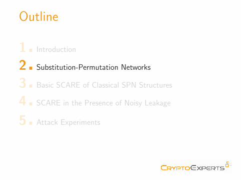
Outline
1 � Introduction
2 � Substitution-Permutation Networks
3 � Basic SCARE of Classical SPN Structures
4 � SCARE in the Presence of Noisy Leakage
5 � Attack Experiments
Outline
1 � Introduction
2 � Substitution-Permutation Networks
3 � Basic SCARE of Classical SPN Structures
4 � SCARE in the Presence of Noisy Leakage
5 � Attack Experiments
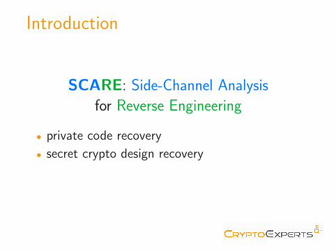
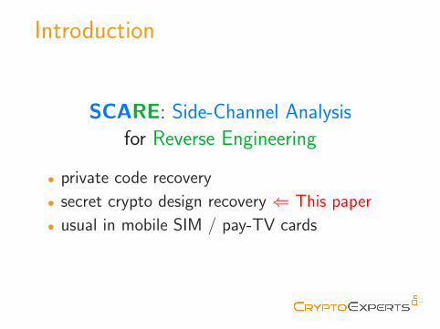
Introduction
SCARE: Side-Channel Analysis
for Reverse Engineering
• private code recovery
• secret crypto design recovery
• usual in mobile SIM / pay-TV cards
Introduction
SCARE: Side-Channel Analysis
for Reverse Engineering
• private code recovery
• secret crypto design recovery ⇐ This paper
• usual in mobile SIM / pay-TV cards
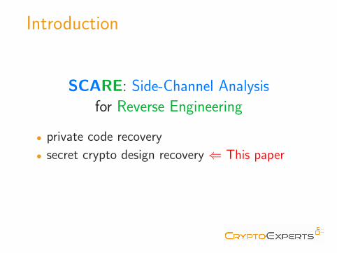
Introduction
SCARE: Side-Channel Analysis
for Reverse Engineering
• private code recovery
• secret crypto design recovery ⇐ This paper
• usual in mobile SIM / pay-TV cards
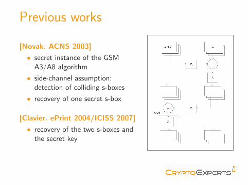
Previous works
[Novak. ACNS 2003]
• secret instance of the GSMA3/A8 algorithm
• side-channel assumption:detection of colliding s-boxes
• recovery of one secret s-box
[Clavier. ePrint 2004/ICISS 2007]
• recovery of the two s-boxes andthe secret key
Limitations
• Target: specific cipher structure
• Assumption: idealized leakage model
⇒ perfect collision detection
Our work
• Consider a generic class of ciphers:Substitution-Permutation Networks (SPN)
• Relax the idealized leakage assumptionI consider noisy leakagesI experiments in a practical leakage model
Further works
[Daudigny et al. ACNS 2005] (DES)
[Real et al. CARDIS 2008] (hardware Feistel)
[Guilley et al. LATINCRYPT 2010] (stream ciphers)
[Clavier et al. INDOCRYPT 2013] (modified AES)
Outline
1 � Introduction
2 � Substitution-Permutation Networks
3 � Basic SCARE of Classical SPN Structures
4 � SCARE in the Presence of Noisy Leakage
5 � Attack Experiments
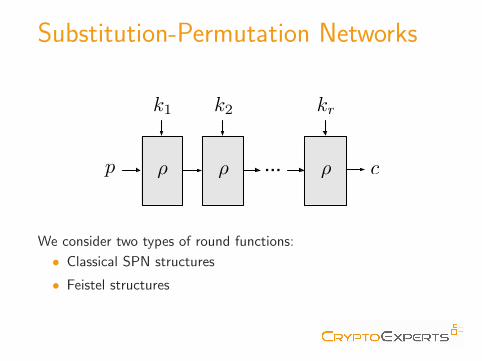
Substitution-Permutation Networks
⇢ ⇢ ⇢
k1 k2 kr
p c...
We consider two types of round functions:
• Classical SPN structures
• Feistel structures
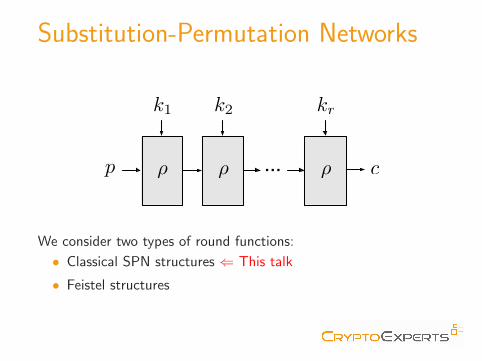
Substitution-Permutation Networks
⇢ ⇢ ⇢
k1 k2 kr
p c...
We consider two types of round functions:
• Classical SPN structures ⇐ This talk
• Feistel structures
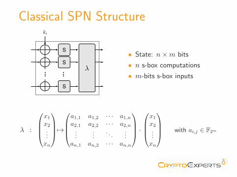
Classical SPN Structure
S
S
S
�
ki
• State: n×m bits
• n s-box computations
• m-bits s-box inputs
λ :
x1x2...xn
7→a1,1 a1,2 · · · a1,na2,1 a2,2 · · · a2,n
......
. . ....
an,1 an,2 · · · an,n
·x1x2...xn
with ai,j ∈ F2m
Outline
1 � Introduction
2 � Substitution-Permutation Networks
3 � Basic SCARE of Classical SPN Structures
4 � SCARE in the Presence of Noisy Leakage
5 � Attack Experiments
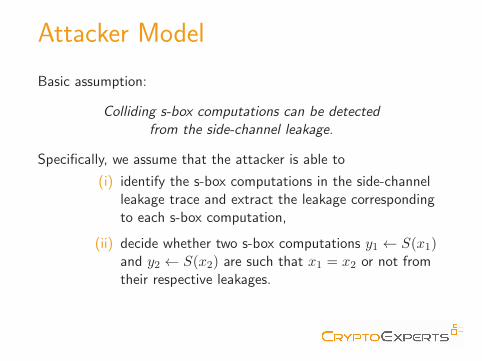
Attacker Model
Basic assumption:
Colliding s-box computations can be detectedfrom the side-channel leakage.
Specifically, we assume that the attacker is able to
(i) identify the s-box computations in the side-channelleakage trace and extract the leakage correspondingto each s-box computation,
(ii) decide whether two s-box computations y1 ← S(x1)and y2 ← S(x2) are such that x1 = x2 or not fromtheir respective leakages.
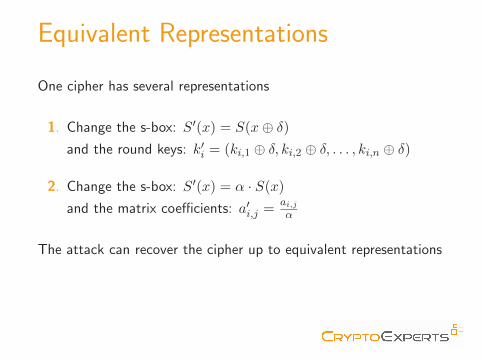
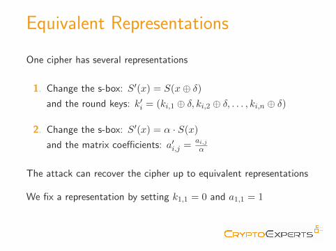
Equivalent Representations
One cipher has several representations
1. Change the s-box: S′(x) = S(x⊕ δ)and the round keys: k′i = (ki,1 ⊕ δ, ki,2 ⊕ δ, . . . , ki,n ⊕ δ)
2. Change the s-box: S′(x) = α · S(x)
and the matrix coefficients: a′i,j =ai,jα
The attack can recover the cipher up to equivalent representations
We fix a representation by setting k1,1 = 0 and a1,1 = 1
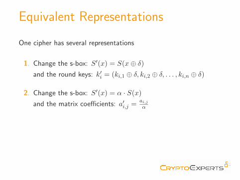
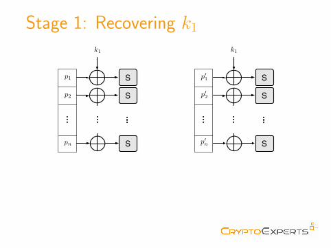
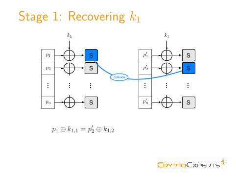
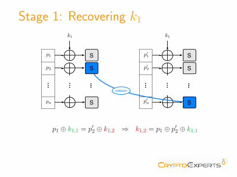
Stage 1: Recovering k1
S
S
S
S
S
S
k1
p1
p2
pn
p01
p02
p0n
k1
⇒ k1,2 = p1 ⊕ p′2 ⊕ k1,1⇒ k1,n = p1 ⊕ p′n ⊕ k1,2
and so on ...

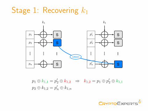
Stage 1: Recovering k1
S
S
S
S
S
S
k1
p1
p2
pn
p01
p02
p0n
k1
collision
⇒ k1,2 = p1 ⊕ p′2 ⊕ k1,1⇒ k1,n = p1 ⊕ p′n ⊕ k1,2
and so on ...
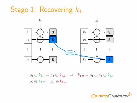
Stage 1: Recovering k1
S
S
S
S
S
S
k1
p1
p2
pn
p01
p02
p0n
k1
collision
p1 ⊕ k1,1 = p′2 ⊕ k1,2
⇒ k1,2 = p1 ⊕ p′2 ⊕ k1,1⇒ k1,n = p1 ⊕ p′n ⊕ k1,2
and so on ...

Stage 1: Recovering k1
S
S
S
S
S
S
k1
p1
p2
pn
p01
p02
p0n
k1
collision
p1 ⊕ k1,1 = p′2 ⊕ k1,2
⇒ k1,2 = p1 ⊕ p′2 ⊕ k1,1⇒ k1,n = p1 ⊕ p′n ⊕ k1,2
and so on ...

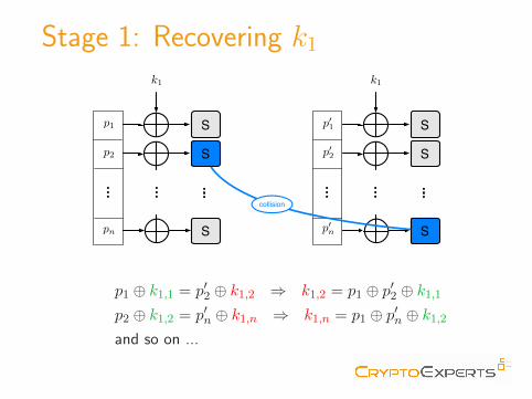
Stage 1: Recovering k1
S
S
S
S
S
S
k1
p1
p2
pn
p01
p02
p0n
k1
collision
p1 ⊕ k1,1 = p′2 ⊕ k1,2 ⇒ k1,2 = p1 ⊕ p′2 ⊕ k1,1
⇒ k1,n = p1 ⊕ p′n ⊕ k1,2and so on ...
Stage 1: Recovering k1
S
S
S
S
S
S
k1
p1
p2
pn
p01
p02
p0n
k1
collision
p1 ⊕ k1,1 = p′2 ⊕ k1,2 ⇒ k1,2 = p1 ⊕ p′2 ⊕ k1,1
⇒ k1,n = p1 ⊕ p′n ⊕ k1,2and so on ...
Stage 1: Recovering k1
S
S
S
S
S
S
k1
p1
p2
pn
p01
p02
p0n
k1
collision
p1 ⊕ k1,1 = p′2 ⊕ k1,2 ⇒ k1,2 = p1 ⊕ p′2 ⊕ k1,1p2 ⊕ k1,2 = p′n ⊕ k1,n
⇒ k1,n = p1 ⊕ p′n ⊕ k1,2and so on ...
Stage 1: Recovering k1
S
S
S
S
S
S
k1
p1
p2
pn
p01
p02
p0n
k1
collision
p1 ⊕ k1,1 = p′2 ⊕ k1,2 ⇒ k1,2 = p1 ⊕ p′2 ⊕ k1,1p2 ⊕ k1,2 = p′n ⊕ k1,n
⇒ k1,n = p1 ⊕ p′n ⊕ k1,2and so on ...
Stage 1: Recovering k1
S
S
S
S
S
S
k1
p1
p2
pn
p01
p02
p0n
k1
collision
p1 ⊕ k1,1 = p′2 ⊕ k1,2 ⇒ k1,2 = p1 ⊕ p′2 ⊕ k1,1p2 ⊕ k1,2 = p′n ⊕ k1,n ⇒ k1,n = p1 ⊕ p′n ⊕ k1,2and so on ...
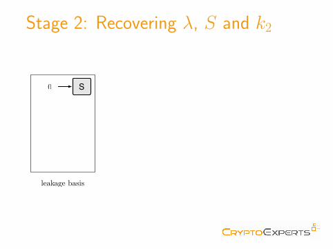
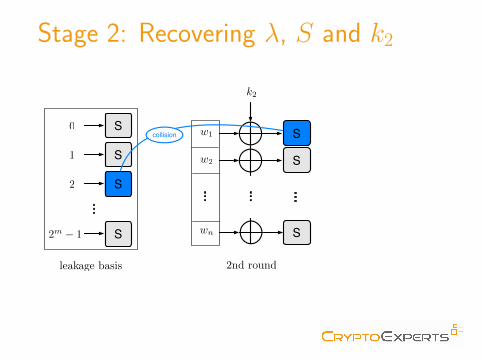
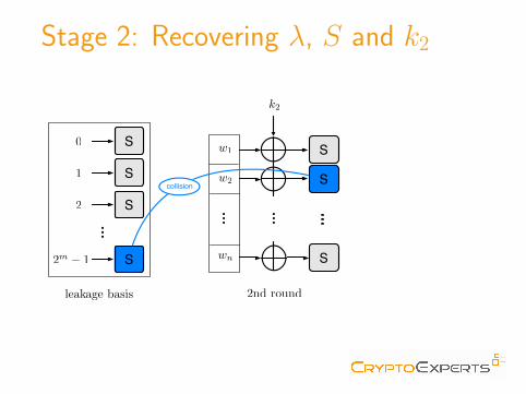
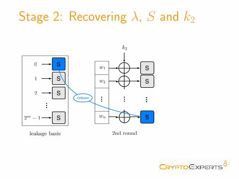
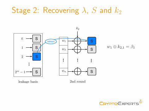
Stage 2: Recovering λ, S and k2
S0
leakage basis
w1 ⊕ k2,1 = β1
w2 ⊕ k2,2 = β2...
wn ⊕ k2,n = βn
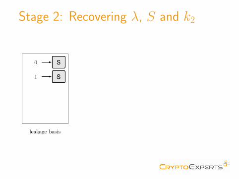
Stage 2: Recovering λ, S and k2
S
S
0
1
leakage basis
w1 ⊕ k2,1 = β1
w2 ⊕ k2,2 = β2...
wn ⊕ k2,n = βn
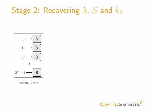
Stage 2: Recovering λ, S and k2
S
S
S
S
0
1
2
2m � 1
leakage basis
w1 ⊕ k2,1 = β1
w2 ⊕ k2,2 = β2...
wn ⊕ k2,n = βn
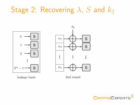
Stage 2: Recovering λ, S and k2
S
S
S
S
0
1
2
2m � 1
S
S
S
w1
w2
wn
k2
leakage basis 2nd round
w1 ⊕ k2,1 = β1
w2 ⊕ k2,2 = β2...
wn ⊕ k2,n = βn
Stage 2: Recovering λ, S and k2
S
S
S
S
0
1
2
2m � 1
S
S
S
w1
w2
wn
k2
leakage basis 2nd round
collision
w1 ⊕ k2,1 = β1
w2 ⊕ k2,2 = β2...
wn ⊕ k2,n = βn
Stage 2: Recovering λ, S and k2
S
S
S
S
0
1
2
2m � 1
S
S
S
w1
w2
wn
k2
leakage basis 2nd round
collision
w1 ⊕ k2,1 = β1
w2 ⊕ k2,2 = β2...
wn ⊕ k2,n = βn
Stage 2: Recovering λ, S and k2
S
S
S
S
0
1
2
2m � 1
S
S
S
w1
w2
wn
k2
leakage basis 2nd round
collision
w1 ⊕ k2,1 = β1
w2 ⊕ k2,2 = β2...
wn ⊕ k2,n = βn

Stage 2: Recovering λ, S and k2
S
S
S
S
0
1
2
2m � 1
S
S
S
w1
w2
wn
k2
leakage basis 2nd round
w1 ⊕ k2,1 = β1
w2 ⊕ k2,2 = β2...
wn ⊕ k2,n = βn
Stage 2: Recovering λ, S and k2
S
S
S
S
0
1
2
2m � 1
S
S
S
w1
w2
wn
k2
leakage basis 2nd round
collision
w1 ⊕ k2,1 = β1
w2 ⊕ k2,2 = β2...
wn ⊕ k2,n = βn
Stage 2: Recovering λ, S and k2
S
S
S
S
0
1
2
2m � 1
S
S
S
w1
w2
wn
k2
leakage basis 2nd round
collision
w1 ⊕ k2,1 = β1
w2 ⊕ k2,2 = β2
...
wn ⊕ k2,n = βn
Stage 2: Recovering λ, S and k2
S
S
S
S
0
1
2
2m � 1
S
S
S
w1
w2
wn
k2
leakage basis 2nd round
collision
w1 ⊕ k2,1 = β1
w2 ⊕ k2,2 = β2...
wn ⊕ k2,n = βn
Stage 2: Recovering λ, S and k2
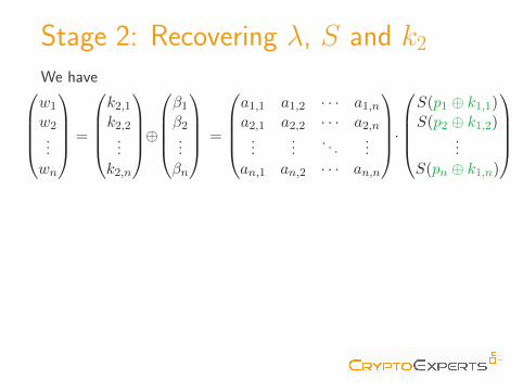
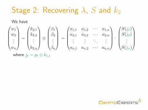
We havew1
w2...wn
=
k2,1k2,2
...k2,n
⊕β1β2...βn
=
a1,1 a1,2 · · · a1,na2,1 a2,2 · · · a2,n
......
. . ....
an,1 an,2 · · · an,n
·S(p1 ⊕ k1,1)S(p2 ⊕ k1,2)
...S(pn ⊕ k1,n)
where jt = pt ⊕ k1,t and xj = S(j).
We get equations of the form:
k2,i ⊕ βi = ai,1 · xj1 ⊕ ai,2 · xj2 ⊕ · · · ⊕ ai,n · xjn
Using linearization, we get a system with 2m · n2 + n unknowns⇒ solvable with 2m · n+ 1 encryptions⇒ solvable with 4097 encryptions for m = 8, n = 16
Stage 2: Recovering λ, S and k2
We havew1
w2...wn
=
k2,1k2,2
...k2,n
⊕β1β2...βn
=
a1,1 a1,2 · · · a1,na2,1 a2,2 · · · a2,n
......
. . ....
an,1 an,2 · · · an,n
·S(j1)S(j2)
...S(jn)
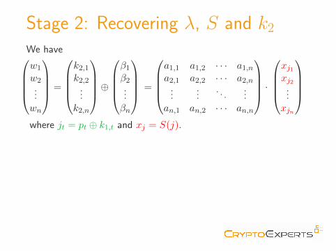
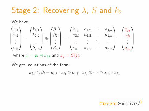
where jt = pt ⊕ k1,t
and xj = S(j).
We get equations of the form:
k2,i ⊕ βi = ai,1 · xj1 ⊕ ai,2 · xj2 ⊕ · · · ⊕ ai,n · xjn
Using linearization, we get a system with 2m · n2 + n unknowns⇒ solvable with 2m · n+ 1 encryptions⇒ solvable with 4097 encryptions for m = 8, n = 16
Stage 2: Recovering λ, S and k2
We havew1
w2...wn
=
k2,1k2,2
...k2,n
⊕β1β2...βn
=
a1,1 a1,2 · · · a1,na2,1 a2,2 · · · a2,n
......
. . ....
an,1 an,2 · · · an,n
·xj1xj2
...xjn
where jt = pt ⊕ k1,t and xj = S(j).
We get equations of the form:
k2,i ⊕ βi = ai,1 · xj1 ⊕ ai,2 · xj2 ⊕ · · · ⊕ ai,n · xjn
Using linearization, we get a system with 2m · n2 + n unknowns⇒ solvable with 2m · n+ 1 encryptions⇒ solvable with 4097 encryptions for m = 8, n = 16
Stage 2: Recovering λ, S and k2
We havew1
w2...wn
=
k2,1k2,2
...k2,n
⊕β1β2...βn
=
a1,1 a1,2 · · · a1,na2,1 a2,2 · · · a2,n
......
. . ....
an,1 an,2 · · · an,n
·xj1xj2
...xjn
where jt = pt ⊕ k1,t and xj = S(j).
We get equations of the form:
k2,i ⊕ βi = ai,1 · xj1 ⊕ ai,2 · xj2 ⊕ · · · ⊕ ai,n · xjn
Using linearization, we get a system with 2m · n2 + n unknowns⇒ solvable with 2m · n+ 1 encryptions⇒ solvable with 4097 encryptions for m = 8, n = 16
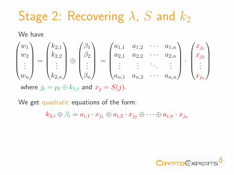
Stage 2: Recovering λ, S and k2
We havew1
w2...wn
=
k2,1k2,2
...k2,n
⊕β1β2...βn
=
a1,1 a1,2 · · · a1,na2,1 a2,2 · · · a2,n
......
. . ....
an,1 an,2 · · · an,n
·xj1xj2
...xjn
where jt = pt ⊕ k1,t and xj = S(j).
We get quadratic equations of the form:
k2,i ⊕ βi = ai,1 · xj1 ⊕ ai,2 · xj2 ⊕ · · · ⊕ ai,n · xjn
Using linearization, we get a system with 2m · n2 + n unknowns⇒ solvable with 2m · n+ 1 encryptions⇒ solvable with 4097 encryptions for m = 8, n = 16
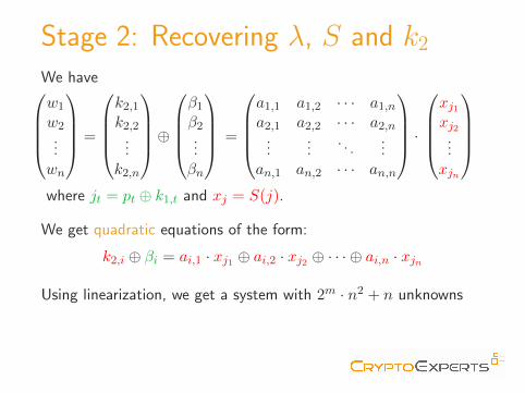
Stage 2: Recovering λ, S and k2
We havew1
w2...wn
=
k2,1k2,2
...k2,n
⊕β1β2...βn
=
a1,1 a1,2 · · · a1,na2,1 a2,2 · · · a2,n
......
. . ....
an,1 an,2 · · · an,n
·xj1xj2
...xjn
where jt = pt ⊕ k1,t and xj = S(j).
We get quadratic equations of the form:
k2,i ⊕ βi = ai,1 · xj1 ⊕ ai,2 · xj2 ⊕ · · · ⊕ ai,n · xjn
Using linearization, we get a system with 2m · n2 + n unknowns
⇒ solvable with 2m · n+ 1 encryptions⇒ solvable with 4097 encryptions for m = 8, n = 16
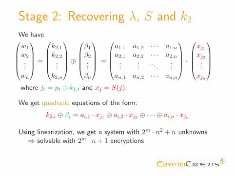
Stage 2: Recovering λ, S and k2
We havew1
w2...wn
=
k2,1k2,2
...k2,n
⊕β1β2...βn
=
a1,1 a1,2 · · · a1,na2,1 a2,2 · · · a2,n
......
. . ....
an,1 an,2 · · · an,n
·xj1xj2
...xjn
where jt = pt ⊕ k1,t and xj = S(j).
We get quadratic equations of the form:
k2,i ⊕ βi = ai,1 · xj1 ⊕ ai,2 · xj2 ⊕ · · · ⊕ ai,n · xjn
Using linearization, we get a system with 2m · n2 + n unknowns⇒ solvable with 2m · n+ 1 encryptions
⇒ solvable with 4097 encryptions for m = 8, n = 16
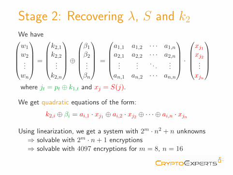
Stage 2: Recovering λ, S and k2
We havew1
w2...wn
=
k2,1k2,2
...k2,n
⊕β1β2...βn
=
a1,1 a1,2 · · · a1,na2,1 a2,2 · · · a2,n
......
. . ....
an,1 an,2 · · · an,n
·xj1xj2
...xjn
where jt = pt ⊕ k1,t and xj = S(j).
We get quadratic equations of the form:
k2,i ⊕ βi = ai,1 · xj1 ⊕ ai,2 · xj2 ⊕ · · · ⊕ ai,n · xjn
Using linearization, we get a system with 2m · n2 + n unknowns⇒ solvable with 2m · n+ 1 encryptions⇒ solvable with 4097 encryptions for m = 8, n = 16
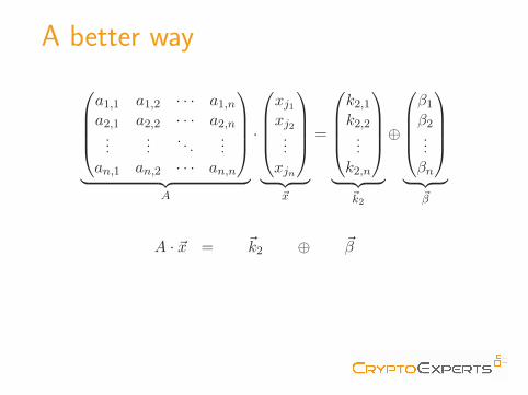
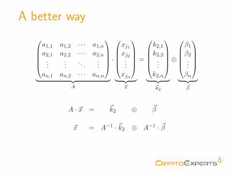
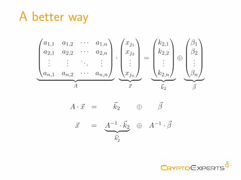
A better way
a1,1 a1,2 · · · a1,na2,1 a2,2 · · · a2,n
......
. . ....
an,1 an,2 · · · an,n
︸ ︷︷ ︸
A
·
xj1xj2
...xjn
︸ ︷︷ ︸
~x
=
k2,1k2,2
...k2,n
︸ ︷︷ ︸
~k2
⊕
β1β2...βn
︸ ︷︷ ︸
~β
A · ~x = ~k2 ⊕ ~β
~x = A−1 · ~k2 ⊕ A−1 · ~β
A better way
a1,1 a1,2 · · · a1,na2,1 a2,2 · · · a2,n
......
. . ....
an,1 an,2 · · · an,n
︸ ︷︷ ︸
A
·
xj1xj2
...xjn
︸ ︷︷ ︸
~x
=
k2,1k2,2
...k2,n
︸ ︷︷ ︸
~k2
⊕
β1β2...βn
︸ ︷︷ ︸
~β
A · ~x = ~k2 ⊕ ~β
~x = A−1 · ~k2 ⊕ A−1 · ~β
A better way
a1,1 a1,2 · · · a1,na2,1 a2,2 · · · a2,n
......
. . ....
an,1 an,2 · · · an,n
︸ ︷︷ ︸
A
·
xj1xj2
...xjn
︸ ︷︷ ︸
~x
=
k2,1k2,2
...k2,n
︸ ︷︷ ︸
~k2
⊕
β1β2...βn
︸ ︷︷ ︸
~β
A · ~x = ~k2 ⊕ ~β
~x = A−1 · ~k2︸ ︷︷ ︸~k′2
⊕ A−1 · ~β
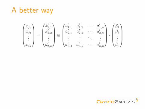
A better way
xj1xj2
...xjn
=
k′2,1k′2,2
...k′2,n
⊕a′1,1 a′1,2 · · · a′1,na′2,1 a′2,2 · · · a′2,n
......
. . ....
a′n,1 a′n,2 · · · a′n,n
·β1β2...βn
We get equations of the form:
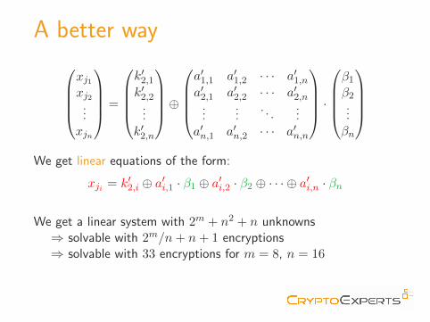
xji = k′2,i ⊕ a′i,1 · β1 ⊕ a′i,2 · β2 ⊕ · · · ⊕ a′i,n · βn
We get a linear system with 2m + n2 + n unknowns⇒ solvable with 2m/n+ n+ 1 encryptions⇒ solvable with 33 encryptions for m = 8, n = 16
A better way
xj1xj2
...xjn
=
k′2,1k′2,2
...k′2,n
⊕a′1,1 a′1,2 · · · a′1,na′2,1 a′2,2 · · · a′2,n
......
. . ....
a′n,1 a′n,2 · · · a′n,n
·β1β2...βn
We get equations of the form:
xji = k′2,i ⊕ a′i,1 · β1 ⊕ a′i,2 · β2 ⊕ · · · ⊕ a′i,n · βn
We get a linear system with 2m + n2 + n unknowns⇒ solvable with 2m/n+ n+ 1 encryptions⇒ solvable with 33 encryptions for m = 8, n = 16
A better way
xj1xj2
...xjn
=
k′2,1k′2,2
...k′2,n
⊕a′1,1 a′1,2 · · · a′1,na′2,1 a′2,2 · · · a′2,n
......
. . ....
a′n,1 a′n,2 · · · a′n,n
·β1β2...βn
We get linear equations of the form:
xji = k′2,i ⊕ a′i,1 · β1 ⊕ a′i,2 · β2 ⊕ · · · ⊕ a′i,n · βn
We get a linear system with 2m + n2 + n unknowns
⇒ solvable with 2m/n+ n+ 1 encryptions⇒ solvable with 33 encryptions for m = 8, n = 16
A better way
xj1xj2
...xjn
=
k′2,1k′2,2
...k′2,n
⊕a′1,1 a′1,2 · · · a′1,na′2,1 a′2,2 · · · a′2,n
......
. . ....
a′n,1 a′n,2 · · · a′n,n
·β1β2...βn
We get linear equations of the form:
xji = k′2,i ⊕ a′i,1 · β1 ⊕ a′i,2 · β2 ⊕ · · · ⊕ a′i,n · βn
We get a linear system with 2m + n2 + n unknowns⇒ solvable with 2m/n+ n+ 1 encryptions
⇒ solvable with 33 encryptions for m = 8, n = 16
A better way
xj1xj2
...xjn
=
k′2,1k′2,2
...k′2,n
⊕a′1,1 a′1,2 · · · a′1,na′2,1 a′2,2 · · · a′2,n
......
. . ....
a′n,1 a′n,2 · · · a′n,n
·β1β2...βn
We get linear equations of the form:
xji = k′2,i ⊕ a′i,1 · β1 ⊕ a′i,2 · β2 ⊕ · · · ⊕ a′i,n · βn
We get a linear system with 2m + n2 + n unknowns⇒ solvable with 2m/n+ n+ 1 encryptions⇒ solvable with 33 encryptions for m = 8, n = 16
And finally
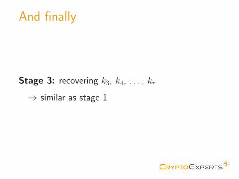
Stage 3: recovering k3, k4, . . . , kr
⇒ similar as stage 1
Outline
1 � Introduction
2 � Substitution-Permutation Networks
3 � Basic SCARE of Classical SPN Structures
4 � SCARE in the Presence of Noisy Leakage
5 � Attack Experiments
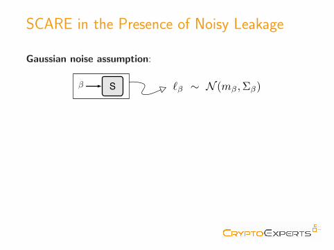
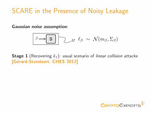
SCARE in the Presence of Noisy Leakage
Gaussian noise assumption:
S� `� ⇠ N (m� ,⌃�)
Stage 1 (Recovering k1): usual scenario of linear collision attacks[Gerard-Standaert. CHES 2012]
Stage 2 (Recovering λ, S and k2) composed of 4 steps:
• building leakage templates• collecting equations• solving a subsystem (Stage 2.1)• recovering remaining unknowns (Stage 2.2)
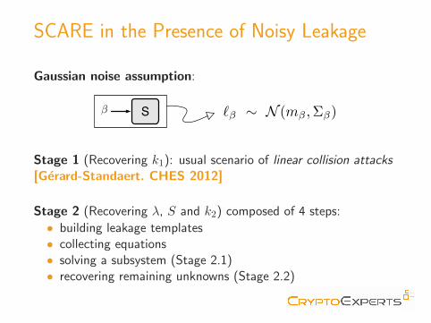
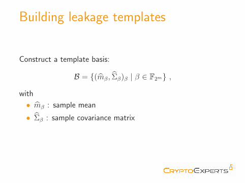
Building leakage templates
Construct a template basis:
B = {(mβ, Σβ)β | β ∈ F2m} ,
with
• mβ : sample mean
• Σβ : sample covariance matrix
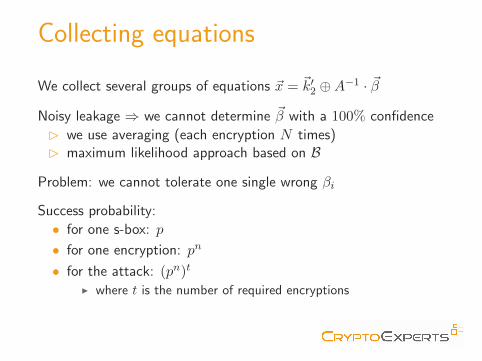
Collecting equations
We collect several groups of equations ~x = ~k′2 ⊕A−1 · ~β
Noisy leakage ⇒ we cannot determine ~β with a 100% confidence
B we use averaging (each encryption N times)B maximum likelihood approach based on B
Problem: we cannot tolerate one single wrong βi
Success probability:
• for one s-box: p
• for one encryption: pn
• for the attack: (pn)t
I where t is the number of required encryptions
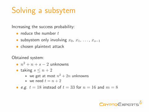
Solving a subsytem
Increasing the success probability:
• reduce the number t
• subsystem only involving x0, x1, . . . , xs−1
• chosen plaintext attack
Obtained system:
• n2 + n+ s− 2 unknowns
• taking s ≤ n+ 2I we get at most n2 + 2n unknownsI we need t = n+ 2
• e.g. t = 18 instead of t = 33 for n = 16 and m = 8
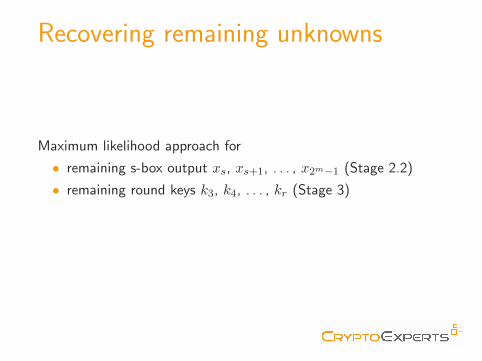
Recovering remaining unknowns
Maximum likelihood approach for
• remaining s-box output xs, xs+1, . . . , x2m−1 (Stage 2.2)
• remaining round keys k3, k4, . . . , kr (Stage 3)
Outline
1 � Introduction
2 � Substitution-Permutation Networks
3 � Basic SCARE of Classical SPN Structures
4 � SCARE in the Presence of Noisy Leakage
5 � Attack Experiments
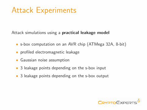
Attack Experiments
Attack simulations using a practical leakage model
• s-box computation on an AVR chip (ATMega 32A, 8-bit)
• profiled electromagnetic leakage
• Gaussian noise assumption
• 3 leakage points depending on the s-box input
• 3 leakage points depending on the s-box output
Attack Experiments
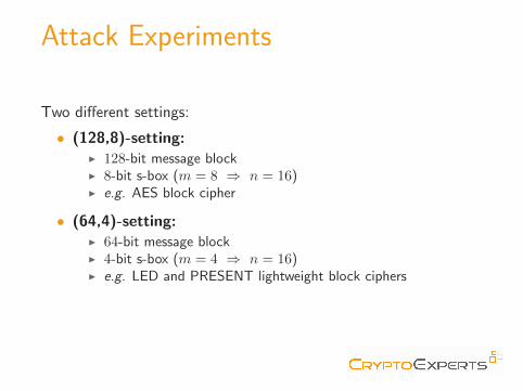
Two different settings:
• (128,8)-setting:I 128-bit message blockI 8-bit s-box (m = 8 ⇒ n = 16)I e.g. AES block cipher
• (64,4)-setting:I 64-bit message blockI 4-bit s-box (m = 4 ⇒ n = 16)I e.g. LED and PRESENT lightweight block ciphers
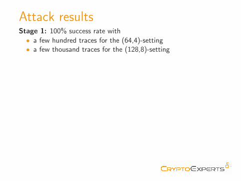
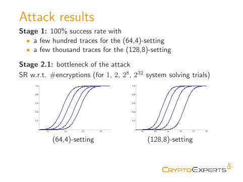
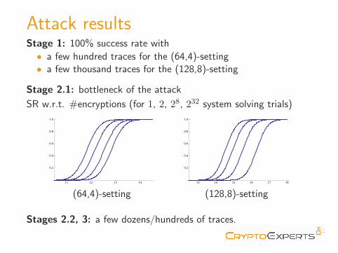
Attack resultsStage 1: 100% success rate with
• a few hundred traces for the (64,4)-setting• a few thousand traces for the (128,8)-setting
Stage 2.1: bottleneck of the attack
SR w.r.t. #encryptions (for 1, 2, 28, 232 system solving trials)
11 12 13 14
0.2
0.4
0.6
0.8
1.0
(64,4)-setting
13 14 15 16 17 18
0.2
0.4
0.6
0.8
1.0
(128,8)-setting
Stages 2.2, 3: a few dozens/hundreds of traces.

The end
Questions?
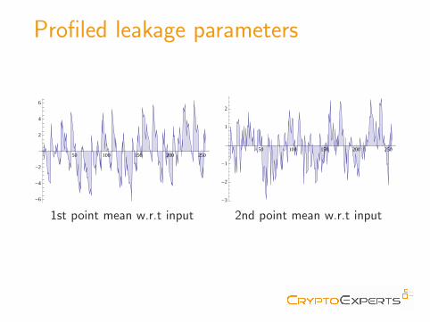
Profiled leakage parameters
50 100 150 200 250
-6
-4
-2
2
4
6
1st point mean w.r.t input
50 100 150 200 250
-3
-2
-1
1
2
2nd point mean w.r.t input
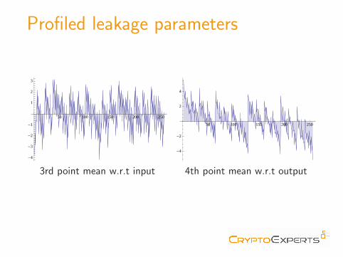
Profiled leakage parameters
50 100 150 200 250
-4
-3
-2
-1
1
2
3
3rd point mean w.r.t input
50 100 150 200 250
-4
-2
2
4
4th point mean w.r.t output
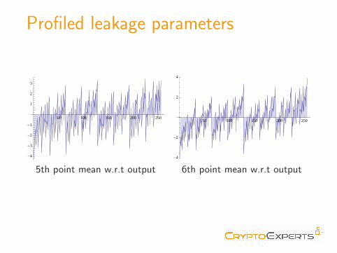
Profiled leakage parameters
50 100 150 200 250
-4
-3
-2
-1
1
2
3
5th point mean w.r.t output
50 100 150 200 250
-4
-2
2
4
6th point mean w.r.t output
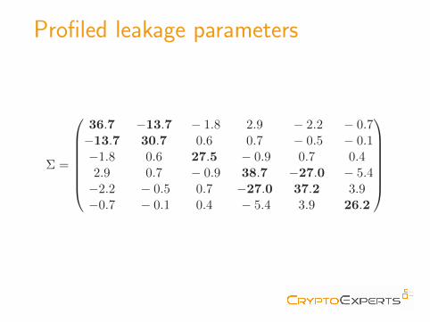
Profiled leakage parameters
Σ =
36.7 −13.7 − 1.8 2.9 − 2.2 − 0.7−13.7 30.7 0.6 0.7 − 0.5 − 0.1−1.8 0.6 27.5 − 0.9 0.7 0.42.9 0.7 − 0.9 38.7 −27.0 − 5.4−2.2 − 0.5 0.7 −27.0 37.2 3.9−0.7 − 0.1 0.4 − 5.4 3.9 26.2