scanning pulse phase thermography with inductive line source · scanning pulse phase thermotgraphy...

Scanning Pulse Phase Thermotgraphy with inductive line source

by B. Oswald-Tranta, M. Sorger

Institute for Automation, University of Leoben, Peter-Tunnerstraße 27, A-8700 Leoben, Austria, [email protected]

Abstract

Thermographical investigation with a line heating source has been carried out, to localize small subsurface defects. The object is moved along an induction coil, used as heating source. The infrared camera records either in reflection or in transmission mode the temperature distribution. From the recorded images the pixel columns are extracted to create a new image sequence. After adjusting the images according to the shift between two consecutive recorded images, the sequence represents the temporal change of the temperature after a short heating pulse. With Fourier transformation a phase image is created, therefore the technique is called scanning pulse phase thermography (SPPT). Finite element simulations and analytical calculations are used to determine the optimal parameters. Experimental results are presented, showing that in reflection mode a 6 mm defect in a 9 mm thick slab in a depth of 7 mm can be detected. In contrast, in transmission mode, even a 4 mm defect in 8 mm depth could be made visible. Keywords: thermography, induction heating, line heating, PPT, SPPT

1. Introduction

In the case of thermographical inspection with line heating, the sample is moving with a constant speed passing in front of the line heat source. The infrared camera records the temperature distribution at the surface in a specified distance after the heating. In the past different groups [1,2,3,4] have shown, that using an optical heat source delaminations, subsurface defects and changes in the sample thickness caused e.g. by corrosion can be detected with this technique. For the evaluation of the measured data one single infrared image has been created from the sequence of the images, extracting only one column of data from the 2D infrared images. In this way the distance between the heat source and the recording position of the temperature values is crucial.

In this paper a new technique is presented, where not only one column is extracted from the recorded images, but all of the columns are used to reconstruct a sequence of infrared images, representing the temporal change of the temperature. From this image sequence a phase image is calculated using the Fourier transformation. The phase image obtained by the presented technique of scanning pulse phase thermography (SPPT) shows even for small holes better resolution than the single temperature images.

2. Experimental setup

In the experiments an inductive line heat source is used. It is much more efficient for the tested metallic materials than optical heating. The heat is induced directly in the sample, therefore the low emissivity does not affect the heating rate. The induction generator works in the high frequency range of 100-200 kHz, therefore the eddy currents are induced only in a thin layer below the surface. For the inspected ferro-magnetic steel samples this thickness is about 0.03 mm. The induction coil and the infrared camera are fixed and the inspected sample is moved along them with a linear actuator. Experiments have been carried out in reflection mode, where the induction coil and the infrared camera are on the same side of the tested object, see Figure 1. Further measurements have been done in transmission mode, the induction coil is positioned below the sample, and the infrared camera records the temperature on the other side of the sample. The triggering of the heating, the camera and the linear motion is controlled and synchronized by a PLC. In the experiments a speed in the range of 0.02-0.2 m/s has been used. The width of the induction coil is 5 mm, therefore the heating duration depending on the speed is in the range of 0.025-0.25 s. As the heating power of the 10 kW generator is adjustable, it was selected so, that in the case of different motion speed always a temperature increase of about 3-10 Degree is achieved in the tested ferro-magnetic samples.

In most of the experiments a cooled infrared camera with InSb detector (camera type: Titanium [5]) has been used with a pixel resolution of 320 x 256. The camera records 385 images pro second. Additional measurements have been carried out using an uncooled microbolometer camera recording only 50 images per second, but with a pixel resolution of 640 x 480 pixels (camera type: Pyroview 640L [6]).

11th International Conference on

Quantitative InfraRed Thermography

Figure 1. Experimental setup: the inspected object is moved by a linear actuator below the

induction coil, and the infrared camera records the temperature distribution behind the coil.

The goal of the experiments was to investigate, in which depth small subsurface defects can be detected by the proposed technique. Therefore, two steel samples with the size of 100 x 200 x 9 mm have been prepared with flat bottom holes. In each of the samples 2 x 6 drillings were created, in one sample with a diameter of 4 and 6 mm and in the other one with 8 and 10 mm. The remaining wall thickness of the drillings is varying from 8 mm up to 3 mm in 1mm steps, see Figure 2.

3mm4mm5mm6mm7mm8mm

9m

m

Figure 2. Sketch of flat bottom hole samples used in the experiments.

3. Conversion of the infrared images

The infrared camera records the temperature distribution either in transmission or in reflection, directly behind the heating, up to a distance of about 15 cm. Figure 3 shows an infrared image recorded in reflection mode, as the moving sample is heated by the induction coil, visible on the left side of the image. Extracting one column of pixels from this infrared image sequence, an image in a specified distance from the heating is created. Using all the pixel columns, and creating from each of them a separate image, generates a new infrared sequence. As the images are created in different positions, the object is shifted between them.

Figure 3. Infrared image of the flat bottom hole sample with 8 and 10 mm diameters, recorded in

reflection mode. The object is moved from the left to the right; on the left side of the image the water cooled induction coil is visible.

The shifting of the object between two consecutive images is determined by using a calibration

target before the series of measurements. With the help of this information the images in the sequence are

11th International Conference on Quantitative InfraRed Thermography, 11-14 June 2012, Naples Italy

shifted to the same position, so that each pixel in the sequence corresponds a real point of the inspected sample. In this way the generated infrared image sequence represents the temporal change of the surface temperature. The generated sequence has as many images, as many pixels the camera has in the motion direction (nx): 320 for our cooled semiconductor detector and 640 for the microbolometer camera. The duration of the whole image sequence, tinspection is defined by the ratio of the camera field of view in the motion direction and by the motion speed. On the other side, the generated images have in the x-direction a number of pixels, which is equal to the number of the recorded images (ntime). This is defined by the product of the inspection duration and of the recording frequency of the camera.

From the calibration target also the correct aspect ratio of the converted images is determined. This aspect ratio depends on the motion speed and it is used in an affine transformation to re-establish the correct x-y ratio of the object.

4. Model calculations

Due to the described conversion an infrared image sequence is available, similar to pulse thermography: after the short heating pulse the temperature decreases rapidly at the surface because of the heat diffusion. The temperature at the surface of a semi-infinite body, which is moving in the x-direction, and passing a fixed heating line source along the y-axis, can be calculated by [7]:

⎟⎟⎠

⎞⎜⎜⎝

⎛⋅⎟

⎠⎞

⎜⎝⎛⋅==

κκπλ 22exp),0( 0

xuKuxqtzTline (1)

where q is the emitted heating rate per unit time per unit length, λ the thermal conductivity, κ the thermal diffusivity, u the motion speed and K0 is the modified Bessel function of the second kind of order zero. The temperature at the surface of a semi-infinite body after a Dirac delta surface heating is described by [7]:

tQtzT instsib π

κλ

== ),0(, (2)

where Q is the applied surface heat amount. After inserting in this equation Q=q/u and t=x/u, it can be compared with Eq.(1), and observed, that the temperature values, due to the high thermal diffusivity of steel, only in the first couple of mm behind the heating are different.

In order to determine the optimal evaluation parameters a finite element simulation model has been setup, using the ANSYS multi-physics simulation package[8]. Figure 4 shows such a simulation model of a flat bottom hole sample. Surface heat flux is applied to the top surface for duration of 0.1 s and the temperature of the top surface is evaluated. The diameter of the defect and its depth is varied and results are compared.

Figure 4. Simulation model with a flat bottom hole

Figure 5a shows the simulated temperature after the pulse heating for defects with a diameter of 8 mm in a depth of 3 up to 8 mm. The height of the model is set to 9 mm correspondingly to the experimentally inspected samples. The depicted temperature values are taken in the centre of the model, in the mid point above the circular defect at the top surface. The absolute contrast, the difference of the temperature above the defect and the temperature at the sound surface is shown in Figure 5b. As comparison the instantaneous heating of the semi-infinite body, see Eq.(2), is also displayed in Figure 5a.


Since in the simulation a short heat pulse of 0.1 s has been applied instead of instantaneous heating, the simulated temperature curves are slightly below the theoretical curve in the first 0.4 s after the heating.

a) b) Figure 5. a: Simulated temperature increase after 0.1 s pulse heating above defects with 8 mm

diameter in depth of 3-8mm.The maximum contrast is marked by ‘+’. Analytically calculated curves of instantaneous heating of a semi-infinite body (‘sib’) and a finite body with 3 and 4 mm thicknesses are also

shown; b: absolute contrast for the same defects as in a). The maximum contrast is marked with ‘+’, the time tw (see Eq.(4)) with ‘*’ and the time tpc (see Eq.(5)) with ‘o’.

As the heat diffusion arrives the back side of a finite body, it reflects back. The reflection coefficient in this case can be taken as 1, since the thermal impedance difference between steel and air is very high. The temperature at the surface of a finite body with thickness d can be described by the equation [7,9]:

( )

( ) ⎥⎦

⎤⎢⎣

⎡⎟⎟⎠

⎞⎜⎜⎝

⎛ −−+=

=⎥⎥⎦

⎤

⎢⎢⎣

⎡⎟⎟⎠

⎞⎜⎜⎝

⎛ −+==

∑

∑∞

=

∞

=

12

22

1

22

,

exp121

42exp21),0(

n

n

ninstfib

tdn

dQ

tdn

tQtzT

κπλκ

κπκ

λ (3)

In Figure 5a two such curves for d=3 mm and d=4 mm are also shown. In the double logarithmical visualization the straight line of the semi-infinite body (see Eq.(2)) tends to be constant at the time of [1]:

πκ

2dtw = (4)

Due to the lateral diffusion the accumulated heat above the defect flows away and the temperature decreases further. As it can be seen in Figure 5a, in the case of small and deep defects the heat flows already away laterally, before the plateau can be arrived. Shepard et al.[10] have shown that the time

πκ2dDt pc

⋅= (5)

can be used to characterize the maximum peak contrast between defect and sound surface temperature. It has been also shown, that if tpc < tw, then due to the lateral heat diffusion the accumulating heat above the defect diminishes earlier, than the plateau can be arrived. That means defects where

2<dD

(6)

can be hardly detected. In Figure 5b, additionally to the maximum of the simulated contrast curves, also tw and tpc are shown. As it can be seen from the curves, there is a difference between the calculated maximum contrast and tpc which can be caused as well by the pulse heating instead of instantaneous heating, as also by the small size of the defects. As D=8 mm, mmDd 65.52/max ≈= , therefore by the last three curves in Figure 5b tpc < tw making difficult to detect these defects.


5. Scanning Pulse Phase Thermography

The generated image sequence, as described in Section 3, is evaluated with the technique of pulse phase thermography (PPT [11]). Figure 6 compares the temperature and phase images of the sample with 8 and 10 mm diameter drillings. The measurement is carried out in reflection with a motion speed of 7.8 cm/s. The temperature image is generated from the pixel column 13.5 cm behind the heating. The holes with the wall thickness of 8-6 mm on the left side of the sample are hardly visible. In the phase image (see Figure 6b), calculated from the same measurement using the presented scanning pulse phase thermography (SPPT), the holes with a remaining wall thickness of 6 mm become much more visible than in the single temperature image. Even the second flat bottom hole from the left side in the second row, with a diameter of 10 mm and with a depth of 7 mm becomes slightly visible. These results are in good agreement with other publications, showing that the phase image has a larger depth resolution, than a single temperature image [12,1].

a) b) Figure 6. Results of reflection measurements on the ferro-magnetic steel sample with drillings of

8 mm (top row) and 10 mm (bottom row) diameters. The remaining wall thickness is decreasing from the left to right from 8 mm to 3 mm in 1 mm steps. a: temperature 1.75 s after the heating; b: phase image

obtained with SPPT.

It is well-known [13,11] that thermal waves with different frequency have different wave length, therefore reflecting with different phase from the back side of the sample and showing different phase patterns at the surface. Maldague et al. [11] have used the phase values of the spectral range obtained by Fourier transformation of the temperature change after the heating pulse. In this case the frequency ranging from the base frequency, corresponding to the inspection duration (f0=1/tinspection), up to the maximal frequency of N/(2 tinspection), where N is the number of the recorded images.

In order to investigate, which inspection time is optimal for the detection of small subsurface defects, we have chosen a different way: the phase has been calculated for different inspection times, using only the base frequency of the Fourier transformation. Figure 7 shows the calculated phase difference between the defect and the sound surface.

Figure 7. Calculated phase difference between a defect (8 mm diameter in a depth of 3-8mm)

and the sound surface depending on the inspection time.

From this figure it can be well seen, that

• At short inspection times (i.e. high frequency thermal waves) the phase above the defect is larger than at the sound surface;

• At one specific inspection time the defect and the sound surface shows the same phase, the corresponding frequency is also called as ‘blind-frequency’;

• Deeper defects show this zero-crossing later;


• At longer inspection times the defective area is characterized by lower phase value than at the sound surface;

• The absolute value of the phase difference for longer inspection times is larger and more constant than before the zero-crossing;

• Deeper lying defects cause smaller phase changes.

Comparing Figure 5b and Figure 7 it can be also noticed, that the maximum of the absolute temperature contrast and the maximum of the phase difference lie in very similar time range. But the detection of defects with PPT can be also done up to longer inspection times, when the phase of the defect is significantly less than the sound surface. Additional simulation results show that the zero crossing depends mainly on the defect depth and increases only slightly with the defect size, see Figure 8. It is to note, that this result is in good agreement with the equation, derived for the phase of a thermal wave interfering in a thin layer [14]. As a thin layer corresponds to an infinite large defect size, it results a slightly higher ‘blind frequency’.

Figure 8. Calculated phase difference between a defect (4-10 mm diameter in a depth of 6 mm)

and the sound surface depending on the inspection time.

6. Comparison of the experimental and calculated results

Figure 9 shows phase images obtained with the SPPT technique for the same sample of flat bottom hole defects with 8 and 10 mm diameters as already shown in Figure 6. It can be well seen, how the phase is changing with the inspection time, as predicted by the calculations. With longer inspection time the phase above the defects becomes less and less compared to the sound surface, resulting in a more significant black pattern. In the last image even the second defects from the left side with 7 mm depth become visible.

a) b)

c) d) Figure 9. Phase images obtained for the same sample as shown in Figure 6 after an inspection

time of 1.8 s (a), 2.5 s (b), 3.5 s (c), 4.95 s (d).


It can be also noticed, that as the phase is changing from positive to negative, a positive (white) ring is visible around the defect, see e.g. in Figure 9a and b the last four defects at the right side. This behaviour can be also recognised in the simulation results, see Figure 10. This simulated defect corresponds in the flat bottom hole sample, the 3rd defect from the right side in the 1st row (diameter 8 mm, depth 5 mm). Comparing the simulated and measured results, an excellent agreement can be recognised. With increasing inspection time the phase difference of the defect is changing from positive to negative. At the inspection time corresponding to the ‘blind frequency’, then the phase difference has a zero value only in the mid point of the defect, but its circumference is further positive, making the defect visible also at the ‘blind frequency’.

a) b) c) d)

Figure 10. Phase images simulated for a defect with 8 mm diameter in 5 mm depth, time duration of the evaluation: 1.8 s (a), 2.5 s (b), 3.5 s (c), 4.95 s (d); for comparison the experimental results of the defect

with the same geometry is shown in Figure 9, in the first row the third bottom hole from the right side.

7. Experimental results with different motion speeds

In the case of SPPT the maximal inspection time is determined by the ratio of the camera field of view in the motion direction and by the motion speed. If the camera field of view is large, then the pixel resolution becomes small. If the motion speed is high, then the inspected object moves too quickly through the range of the camera. Therefore the optimum of these two parameters has to be found for an experimental setup.

Is the motion speed slow, then the inspection time is long and the defects become visible through the negative phase difference. Figure 11 shows results of SPPT experiments with 0.05 m/s speed, the inspection time is 6 s. The sample has smaller defects than the previous samples: 6 mm diameter in the first row and 4 mm in the second row. Their depths are again 3-8 mm from the right side to the left. In the first row, except the shallowest defect, all of them can be recognised, even in the depth of 7 mm. In this case D/d = 6/7~ 0.85, which is much less than 2 , as according to Eq.(6) the limit for the detectability was.

Figure 11. Phase image of the sample with 6 mm (first row) and 4 mm (second row) flat bottom

holes, motion speed = 0.05 m/s.

Is the speed higher, then the inspection time becomes shorter. In this case most of the defects have a larger phase value than the sound surface, therefore they can be well detected. Figure 12 shows SPPT results for the sample with 8 and 10 mm defects, measured with a speed of 0.156 m/s and 0.208 m/s, where the inspection time was 2 s and 1.53 s, respectively. The contrast of the defects becomes less with higher motion speed, because of the shorter inspection time, but defects with 8 and 10 mm diameter up to a depth of 5 mm can be reliably detected, which corresponds to a ratio of D/d=8/5=1.6.


a) b) Figure 12. Phase images of the sample with 8 mm (first row) and 10 mm (second row) flat bottom

holes; a: motion speed = 0.156 m/s, b: motion speed = 0.208 m/s.

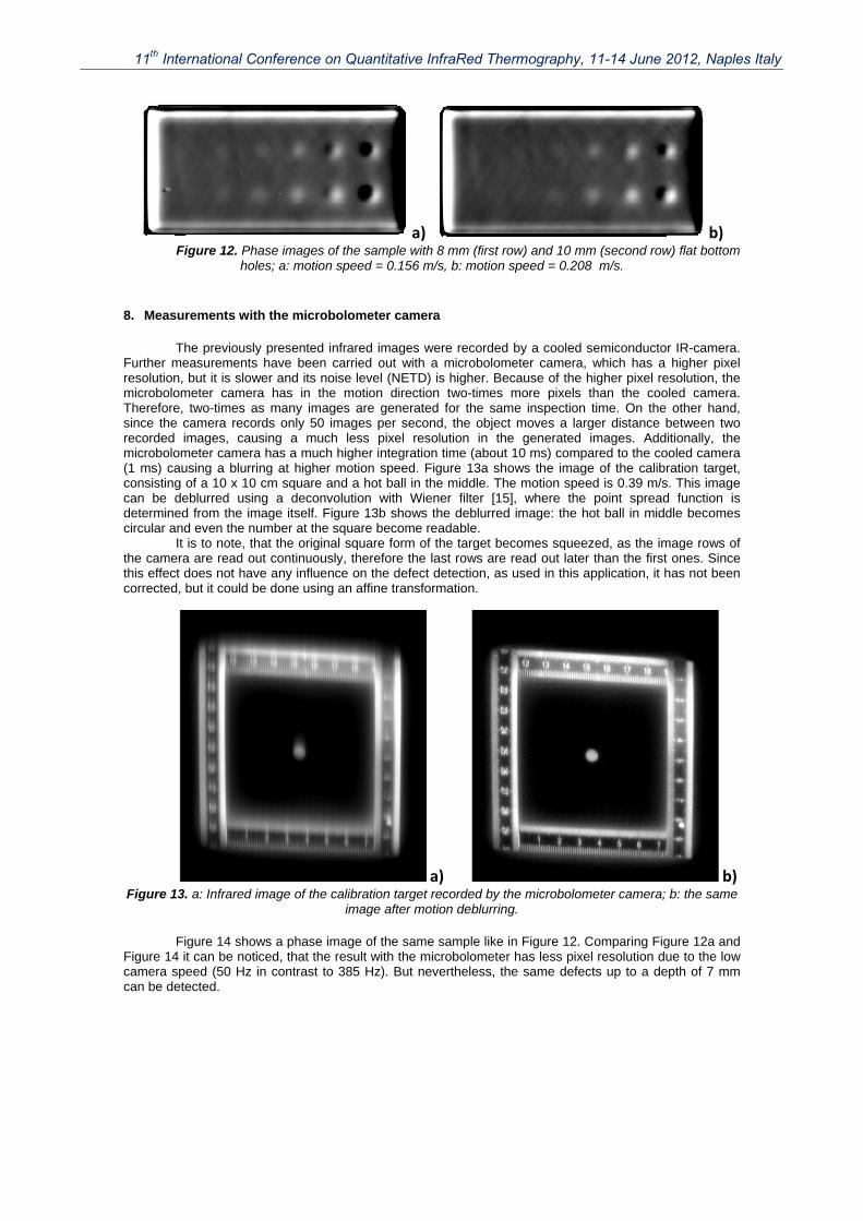
8. Measurements with the microbolometer camera

The previously presented infrared images were recorded by a cooled semiconductor IR-camera. Further measurements have been carried out with a microbolometer camera, which has a higher pixel resolution, but it is slower and its noise level (NETD) is higher. Because of the higher pixel resolution, the microbolometer camera has in the motion direction two-times more pixels than the cooled camera. Therefore, two-times as many images are generated for the same inspection time. On the other hand, since the camera records only 50 images per second, the object moves a larger distance between two recorded images, causing a much less pixel resolution in the generated images. Additionally, the microbolometer camera has a much higher integration time (about 10 ms) compared to the cooled camera (1 ms) causing a blurring at higher motion speed. Figure 13a shows the image of the calibration target, consisting of a 10 x 10 cm square and a hot ball in the middle. The motion speed is 0.39 m/s. This image can be deblurred using a deconvolution with Wiener filter [15], where the point spread function is determined from the image itself. Figure 13b shows the deblurred image: the hot ball in middle becomes circular and even the number at the square become readable.

It is to note, that the original square form of the target becomes squeezed, as the image rows of the camera are read out continuously, therefore the last rows are read out later than the first ones. Since this effect does not have any influence on the defect detection, as used in this application, it has not been corrected, but it could be done using an affine transformation.

a) b) Figure 13. a: Infrared image of the calibration target recorded by the microbolometer camera; b: the same

image after motion deblurring.

Figure 14 shows a phase image of the same sample like in Figure 12. Comparing Figure 12a and Figure 14 it can be noticed, that the result with the microbolometer has less pixel resolution due to the low camera speed (50 Hz in contrast to 385 Hz). But nevertheless, the same defects up to a depth of 7 mm can be detected.


Figure 14. Phase image of the sample with 8 and 10 mm flat bottom holes generated with SPPT using a microbolometer camera; motion speed is 0.13 m/s and inspection time is 2.3 s.

9. Measurements in transmission mode

In transmission mode the induction coil is placed below the inspected object, which is moved by the linear actuator, and the infrared camera records the temperature of the top surface. In order to determine the optimal parameters for this type of measurement, the same simulation model has been used, as shown in Figure 4, but this time the surface heat flux is applied to the bottom surface. This model assumes a homogeneous heating at the bottom surface, as well as at the bottom of the flat hole, which is a good estimation for the real measurements. Figure 15 shows the simulated temperature increase above the same defects, as shown already in reflection mode in Figure 5, and the temperature difference between defect and sound surface.

a) b) Figure 15. a: Simulated temperature increase after 0.1 s pulse heating in transmission mode

above defects with 8 mm diameter in depth of 3-8 mm; b: absolute contrast for the same defects as in a). The maximum contrast is marked in both figures by ‘+’.

Comparing the time-temperature curves for reflection and transmission mode, see Figure 5b and Figure 15b, the position of the maximum values for the transmission are significantly lower and for the different defect sizes and positions much closer together. This is well understandable, as in transmission mode the heat diffusion has only the distance between bottom and top, and in reflection mode the distance is twice as long. Therefore the blurring effect of the heat diffusion is also less in transmission. Figure 16 shows measurement results for 4, 6, 8 and 10 mm diameter defects. As it can be seen, even the smallest and deepest defect becomes visible, where the ratio D/d = 4mm/8mm = 0.5 is significantly below the detectability limit in the reflection mode.

a) b) Figure 16. Phase image of the samples in transmission with 8 mm and 10 mm (a) and with 4 mm

and 6 mm (b) flat bottom holes; motion speed = 0.13 m/s, inspection time= 1s.


10. Summary

The new technique of scanning pulse phase thermography (SPPT) with inductive line heating has been presented. The inspected object is moved along the induction coil and the infrared camera records either on the same side or on the other side the temperature distribution. From the recorded infrared image sequence a new sequence is generated, extracting the pixel columns and shifting according to the motion between two consecutive images. In the case of a microbolometer camera and higher motion speed, the motion blurring effect has to be eliminated additionally, to get sharper images.

From the generated image sequence a phase image is created using Fourier transformation. Flat bottom hole samples with defects from 4 up to 10 mm size and in a depth of 3 up to 8 mm has been used, to demonstrate the advantages of the technique, compared to evaluate a single temperature image. Finite element simulations have been used to determine the optimal inspection time for the reflection and for the transmission mode. In reflection mode, if the motion speed is high, that means the inspection time is short, than defects with a size of 8 mm up to a depth of 5 mm are visible, as their phase is larger than that of the sound surface. Is the motion speed lower, the inspection time becomes longer, and the defects become visible due to lower phase values. Even smaller defects with a size of 6 mm in a depth of 7 mm can be detected.

Experiments in transmission mode cannot be always carried out, if the sample is not in accessible on both sides. But if it is possible, then much smaller defects with a size of 4 mm up to a depth of 8 mm could be made visible with the presented technique.

REFERENCES

[1] Maldague X., Theory and Practice of Infrared Technology for Nondestructive Testing, John Wiley & Sons, Inc. 2001.

[2] Cramer K. E., Winfree W. P., Thermal characterization of defects in aircraft structures via spatially controlled heat application, Proc. SPIE 2766, Thermosense XVIII, 202-209 (1996).

[3] Cramer K. E., Winfree W. P., Thermographic Detection and Quantitative Characterization of Corrosion by Application of Thermal Line Source, Proc. SPIE 3361, Thermosense XX, 291-300 (1998).

[4] Bison P., Marinetti S., Cuogo G., Molinas B., Zonta P., Grinzato E., Corrosion detection on pipelines by IR thermography, in Proc. SPIE 8013, Thermosense XXXIII (2011).

[5] FLIR Systems, Inc., http://www.flir.com [6] DIAS Infrared GmbH, http://www.dias-infrared.com [7] Carslaw H.S., Jaeger J.C., Conduction of Heat in Solids, Oxford University Press, Oxford, 1959. [8] ANSYS Inc., http://www.ansys.com [9] Parker W.J., Jenkins R.J., Butler C.P., Abbott G.L., Flash method of determining thermal

diffusivity, heat capacity and thermal conductivity, J. Applied Physics, Vol. 32, pp. 1679-1684, Sept. 1961.

[10] Shepard S. M., Lhota J. R., Ahmed T., Flash thermography contrast model based on IR camera noise characteristics, J. Nondestructive Testing and Evaluation, 2007.

[11] Maldague X., Marinetti S., Pulse Phase Infrared Thermography, J. Appl.Phys., Vol. 79, No. 5, pp. 2694-2698, 1996.

[12] Busse G., Wu D., Karpen W., Thermal wave imaging with phase sensitive modulated thermography, J. Appl. Phys. 71(8), 1992.

[13] Busse G., Optoacoustic phase angle measurement for probing a metal, Appl.Phys.Lett. 35(10) pp. 759-760, 1979.

[14] Almond D., Patel P., Photothermal Science and Techniques. Chapman & Hall, 1996. [15] Oswald-Tranta B., Sorger M., O’Leary P., Motion deblurring of infrared images from a

microbolometer camera, Journal of Infrared Phys. & Technol., vol. 53, no. 4, pp. 274–279, 2010.


scanning pulse phase thermography with inductive line source · scanning pulse phase thermotgraphy...

Documents