Scaling of strength and lifetime probabilitydistributions of quasibrittle structures basedon atomistic fracture mechanicsZdenek P. Bažanta,1, Jia-Liang Lea, and Martin Z. Bazantb

aDepartment of Civil Engineering and Materials Science, Robert R. McCormick School of Engineering and Applied Science, Northwestern University,Evanston, IL 60208-3109; and bDepartment of Chemical Engineering, Massachusetts Institute of Technology, Cambridge, MA 02139-4307;

Contributed by Zdenek P. Bažant, April 30, 2009 (sent for review January 27, 2009)

The failure probability of engineering structures such as aircraft,bridges, dams, nuclear structures, and ships, as well as microelec-tronic components and medical implants, must be kept extremelylow, typically <10−6. The safety factors needed to ensure it haveso far been assessed empirically. For perfectly ductile and perfectlybrittle structures, the empirical approach is sufficient because thecumulative distribution function (cdf) of random material strengthis known and fixed. However, such an approach is insufficient forstructures consisting of quasibrittle materials, which are brittlematerials with inhomogeneities that are not negligible comparedwith the structure size. The reason is that the strength cdf of quasib-rittle structure varies from Gaussian to Weibullian as the structuresize increases. In this article, a recently proposed theory for thestrength cdf of quasibrittle structure is refined by deriving it fromfracture mechanics of nanocracks propagating by small, activation-energy-controlled, random jumps through the atomic lattice. Thisrefinement also provides a plausible physical justification of thepower law for subcritical creep crack growth, hitherto consideredempirical. The theory is further extended to predict the cdf of struc-tural lifetime at constant load, which is shown to be size- andgeometry-dependent. The size effects on structure strength andlifetime are shown to be related and the latter to be much stronger.The theory fits previously unexplained deviations of experimen-tal strength and lifetime histograms from the Weibull distribution.Finally, a boundary layer method for numerical calculation of thecdf of structural strength and lifetime is outlined.

cohesive fracture | crack growth rate | extreme value statistics | size effect |multiscale transition

A comprehensive theory of the statistical strength distributionexists only for perfectly brittle structures failing at macro-

crack initiation from a negligibly small representative volumeelement (RVE) of material. The objective of the present articleis to extend recent studies (1–3) by developing a comprehensiveand atomistically based theory for strength and lifetime distri-butions of structures consisting of quasibrittle materials. Thesematerials, which include fiber composites, concretes, rocks, stiffsoils, foams, sea ice, consolidated snow, bone, tough industrialand dental ceramics, and many other materials on approach tonanoscale, are characterized by a RVE that is not negligible com-pared with structure size D. The space does not allow commentingon previous valuable contributions made by Coleman (4), Zhurkov(5, 6), Freudenthal (7), Phoenix (8, 9) and others (10, 11) (for suchcomments, see, e.g., refs. 2, 3, 12, and 13).

Fracture Kinetics on Atomic Scale. Consider a nano-scale sizeatomic lattice block undergoing fracture (Fig. 1A). The separationδ between the opposite atoms across the crack gradually increasesby smallincrements as the distance from the crack front grows.The work of the force Fb transmitted across each pair of oppo-site atoms on their relative displacement δ defines a certain localpotential Π1(δ), which is a part of the overall potential function Π(or free energy) of the atomic lattice block. The equilibrium states

of these atomic pairs (bonds) are marked on the local potentialcurves Π1(δ) by circles. As the fracture separation grows from oneatomic pair to the next, the state marked by the circle moves on thecurve Π1(δ) up and right (Fig. 1B). These states are also shown onthe corresponding curves of bond force Fb(δ) = ∂Π1/∂δ betweenthe opposite atoms in each pair (Fig. 1C). The local bond failurebegins when the peak point of the curve Fb(δ) is reached. Thispoint corresponds to the point of maximum slope of the curveΠ1(δ) (state 3), and represents the end of the cohesive crack [anold idea attributed to Barenblatt (14)]. The true crack ends at thepair where the bond force is reduced to 0 (state 1).

The fracture process zone (FPZ) in the lattice spans approxi-mately from state 1 to state 3, which lies many atoms apart. As thefracture propagates, the diagram P(u) of load P = ∂Π/∂u appliedon the atomic lattice block versus the associated displacement ucaused by elasticity of lattice and by fracture growth would havethe usual shape shown in Fig. 1D if the lattice were treated as acontinuum (the curvature of the rising portion is caused by finite-ness of the length of growing FPZ). On the nanoscale, however,the lattice is not a continuum. The fracture advances by randomjumps over the activation energy barriers Q on the surface of thestate potential Π (free energy) of the atomic lattice block. Thesebarriers cause the diagram P(u) to be wavy; see Fig. 1E, wherethe radial lines marked as a1, a2, . . . correspond to the unloadinglines for subsequent crack lengths ending at different atomic pairsmarked in Fig. 1A.

The interatomic crack propagates by jumps equal to the atomicspacing δa. During each jump, one barrier on the potential Π asa function of u must be overcome (see the wavy potential profilein Fig. 1G). After each jump, at each new crack length, there is asmall decrease (Fig. 1 F and G) of the overall potential Π of theatomic lattice block, corresponding to a small advance along theload-deflection curve P(u) (Fig. 1 E). An important point is thatthe separation of opposite atoms (in their equilibrium positions)increases during each jump by only a small fraction of their initialdistance δa.

Because of thermal activation, the states of the atomic latticeblock fluctuate and can jump over the activation energy barrier ineither direction (forward of backward, Fig. 1F), although not withthe same frequency. When crack length a (defined by the locationof state 3 in Fig. 1 A–C) jumps by one atomic spacing, i.e, from aito ai + δa, i = 1, 2, 3, . . .), the activation energy barrier Q changesby a small amount, ΔQ, corresponding to the energy release byfracture (Fig. 1 F and G) that is associated with the equilibriumload drop P caused by fracture (Fig. 1 E).

To calculate ΔQ, consider planar 3-dimensional cracks thatgrow in an affine, or self-similar, manner (e.g., expandingconcentric circles or squares). The FPZ of the lattice crack cannotbe expected to be negligible compared with the size la of the atomic

Author contributions: Z.P.B. designed research; Z.P.B., J.-L.L., and M.Z.B. performedresearch; J.-L.L. analyzed data; and Z.P.B. and J.-L.L. wrote the paper.

The authors declare no conflict of interest.1To whom correspondence should be addressed. E-mail: z-bazant@northwestern.edu.

11484–11489 PNAS July 14, 2009 vol. 106 no. 28 www.pnas.org / cgi / doi / 10.1073 / pnas.0904797106

Dow

nloa

ded

by g

uest

on

May

18,

202

0

ENG

INEE

RIN

G

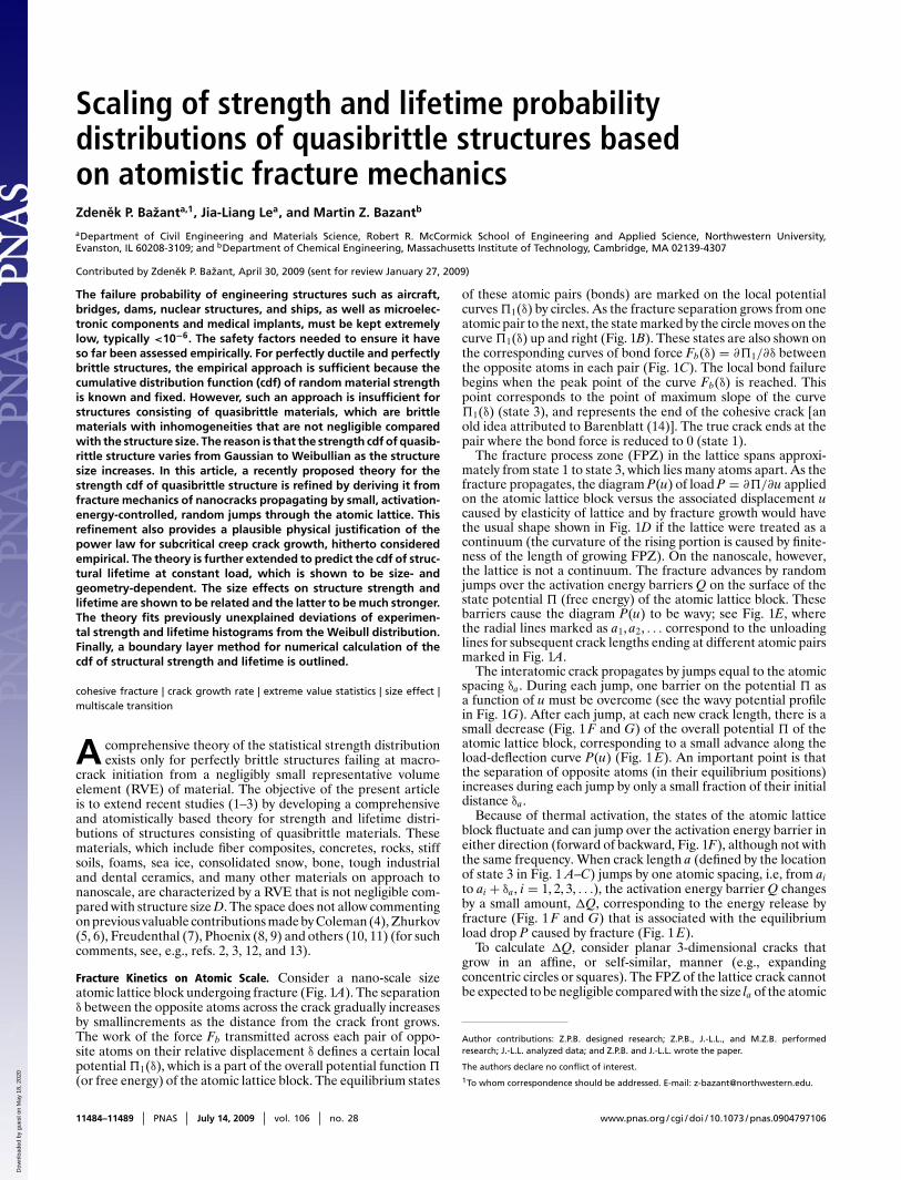
Fig. 1. Nanoscale fracture and fits of histograms. (A–C) Fracture of atomic lattice. (D–G) Load-displacement curve of atomic lattice block. (H–K) Optimumleast-squares fits of experimental strength histograms by the present theory and the 2-parameter Weibull distribution: (H) Sintered Si3N4 with CTR2O3/Al2O3

additives, (I) sintered Si3N4-Al2O3-Y2O3, (J) Vitadur Alpha Core, (K) Leucite-reinforced porcelain. (L–O) Optimum least-squares fits of experimental lifetimehistograms of Kevlar 49 fiber composites by the present theory and the 2-parameter Weibull distribution. (P) Problematic subdivision for curved boundary. (Q)Nonlocal boundary layer model.

lattice block, and so we will use the approximation of equivalentlinear elastic fracture mechanics (LEFM) in which the tip of anequivalent sharp LEFM crack is considered to lie approximately inthe middle of the FPZ. The LEFM stress intensity factor (of modeI, II, or III) is in general expressed as Ka = τ

√laka(α), where

α = a/la = relative crack length, ka(α) = dimensionless stressintensity factor, τ = cσ = remote stress applied on the nanoscaleon the atomic lattice block of size la (Fig. 1A); c is a nano-macrostress concentration factor; and σ = macroscale stress in the RVE.For a circular (or penny-shaped) crack of radius a loaded in modeI by a remote stress, ka(α) = √

4α/π.The energy release rate of the crack (with respect to crack

length rather than time), per unit length of crack perimeter, isGa(α) = K2

a /E1 = k2a(α) laτ2/E1. Here E1 = Young’s (elastic)

modulus for a continuum approximation of the lattice (which is

larger than the macroscopic Young’s modulus E); k2a(α) repre-

sents the dimensionless energy release rate function of LEFM forcontinuous bodies, characterizing the geometry of fracture and ofthe atomic lattice block (15) (if the block boundaries are distant,k2

a(α) ∝ γα). Let γ1 = geometry constant such that γ1a = γ1αla =crack perimeter, the crackbeing assumed to grow radially in anaffine manner (γ1 = 2π for a circular crack of radius a = αla, andγ1 = 8 for a square perimeter crack). Similar to the expression inref. 3 (derived by assuming 2- rather than 3-dimensional cracks),the increment of energy that is released when the crack advancesby δa along its entire perimeter of length γ1αla is:

ΔQ = δa

[∂Π∗(P, a)

∂a

]P

= δa(γ1αla)Ga = Va(α)τ2

E1[1]

Bažant et al. PNAS July 14, 2009 vol. 106 no. 28 11485

Dow

nloa

ded

by g

uest

on

May

18,

202

0

Here, Π∗ = complementary energy potential (Gibbs’ free energy)of the atomic lattice block, and Va(α) = δa(γ1αl2

a)k2a(α) = activa-

tion volume. [Note that if the stress tensor is written as τ s, whereτ = stress parameter, one may write Va = s : va, where va =activation volume tensor, as in the atomistic theories of phasetransformations in crystals (16).]

Because the cohesive crack is much longer than δa, the separa-tion δ changes very little during each crack jump by one atomicspacing δa, and so the activation energy barrier for a forward jump,Q0 − ΔQ/2, differs very little from the activation energy barrierfor a backward jump, Q0 + ΔQ/2 (Q0 = activation energy atno stress) (Fig. 1F). Note that multiple activation energy barri-ers Q0 = Q1, Q2, . . . are always present; however, the lowest onealways dominates. The reason is that the factor e−Q1/kT is verysmall, typically 10−12 (e.g., if Q2/Q1 = 1.2 or 2, then e−Q2/kT =0.0043e−Q1/kT or 10−23e−Q1/kT and thus makes a negligible con-tribution; and if Q2/Q1 = 1.02, then Q1 and Q2 can be replacedby a single activation energy Q0 = 1.01Q1). Consequently, thejumps from one metastable state to the next on the surface ofthe atomic lattice block potential Π∗ must be happening in bothforward and backward directions, although at slightly differentfrequencies. According to the transition rate theory (17, 18), thefirst-passage time for each transition (in the limit of a large free-energy barrier, Q0 � kT) is given by Kramer’s formula (19). Thus,the net frequency of crack length jumps is (3):

f1 = νT (e(−Q0+ΔQ/2)/kT − e(−Q0−ΔQ/2)/kT ) [2]

= 2νT e−Q0/kT sinh[Va(α)/VT ] [3]

where VT = 2E1kT/τ2; νT is the characteristic attempt frequencyfor the reversible transition, νT = kT/h, where h = 6.626 ·10−34 Js = Planck constant = (energy of a photon)/(frequencyof its electromagnetic wave); T = absolute temperature; and k =1.381 ·10−23 J/K = Boltzmann constant. Since δa is of the order of0.1 nm, Va ∼ 10−26 m3. Volume VT depends on τ = cσ where c isexpected to be>10. For example, in the nanostructure of hardenedPortland cement gel, the nanoscale remote stress may perhapsbe τ ≈ 20 MPa, which gives VT ∼ 10−25 m3, and so Va/VT �1. Therefore, Eq. 3 becomes f1 ≈ e−Q0/kT [νT Va(α)/kT]τ2/E1.Denoting HT = e−Q0/kT (δal2

a/E1h) and FT = γ1αk2a(α)HT , we

thus have:

f1 = FTτ2 [4]

The fact that frequency f1 is a power law of stress τ with azero threshold is essential for the forthcoming arguments. Impor-tant for the foregoing derivation is that ΔQ � kT � Q0 orτ � (E1kT/Va)1/2. Another noteworthy point is that stress-independent crack front diffusion (as a random walk) should benegligible because the Péclet number Pe � 1 [Pe = 2f1la/δaf =4(la/δa)(Va/VT ), where f = νT e−Q0/kT ].

In classical macroscale continuum fracture, by contrast, thejumps representing fracture reversal play no role because thecrack face separations of interest equal many atomic spacings,rather than a small fraction of one atomic spacing; ΔQ is thusentirely negligible and the free-energy change is smooth (as shownin Fig. 1G) (this point was made in ref. 20, figure 1.18).

Failure Frequency and Probability at Nanoscale. The atomic latticefails when the nanocrack propagates from its original length a0to a certain critical length ac at which the crack looses stabil-ity and propagates dynamically [this occurs at the point of theP(u) curve in Fig. 1E where the downward tangent slope becomesequal in magnitude to the stiffness of embedment of the latticeblock in the surrounding microstructure (21)]. To get to ac, thecrack experiences many length jumps, say n jumps, where the fre-quency of each jump is given by Eq. 4. At the atomic lattice scale,it may be assumed, in general, that each jump is independent

(i.e., the frequency of the jump is independent of the particu-lar history of breaking and restoration sequences that brought thenanocrack to the current length) (20). The failure probability ofthe atomic lattice on sudden application of stress can thus be writ-ten as Pf (τ) ∝ limn→∞

∑ni=1 f1(i) = ∫ αc

α0f1dα, where f1(i) = value

of f1 for crack length a(i) ending at interatomic bond number i.Denoting CT = HTγ1

∫ αcα0

αk2a(α)dα, we thus get

Pf (τ) ∝ CTτ2 [5]

Nano-Macro Transition of Failure Probability. We consider the broadclass structures that fail as soon as a macrocrack initiates from oneRVE (15, 22, 23) (they are called the positive geometry structures,characterized by ∂K/∂a > 0; K = stress intensity factor). Theirstrength is statistically modeled by a chain of RVEs, i.e., by theweakest-link model. However, in contrast to Weibull theory, thenumber of RVEs (or links in the chain) is not infinite becausethe RVE size is not negligible. For softening damage and failure,and in contrast to the homogenization theory, the RVE must bedefined as the smallest material volume whose failure triggers thefailure of the whole structure (1). Typically, the RVE size l0 is ≈2to 3 inhomogeneity sizes (2, 25).

The transition from the nanoscale of atomic lattice crack to themacroscale of RVE can be represented, for statistical purposes, bya hierarchy of series and parallel couplings (i.e., chains of links andbundles of fibers) (see ref. 1, figure 1E). In such couplings, a powerlaw tail of strength cumulative distribution function (cdf) is inde-structible (2). The series couplings preserve the tail exponent andextend the reach of the power-law tail. In parallel couplings, thetail exponents of the elements are additive [as proven for both brit-tle (2, 24) and plastic or softening elements (2)], and the reach ofthe power-law tail shortens drastically. The cdf of strength of oneRVE can be approximated by a Gaussian core onto which a far-leftWeibull tail is grafted at failure probability Pgr ≈ 10−4 −10−3 (ref.1, equations 6 and 7) [in more detail (2)]. The meaning of Weibullmodulus m, which is typically 10 to 50, is the minimum of the sumof the Weibull tail powers among all possible cuts separating thehierarchical model into two halves.

The elements of the hierarchical model may be imagined to rep-resent atomic lattice cracks, for which the tail exponent of strengthcdf is 2 (Eq. 5). Isn’t that in conflict with the preceding simplermodel (1), in which the elements of the hierarchical model hadthe tail exponent of 1? No, because the elements in ref. 1 repre-sented the break of a bond between a pair of atoms, which occursone scale lower than the break of atomic lattice block. Accord-ing to the hierarchical model, the passage from that scale to thescale of atomic lattice should raise the exponent, and the presentanalysis shows it should raise it to 2. Although refs. 1 and 2 led toequivalent results on the RVE level, the treatment of interatomicpair breaks in refs. 1 and 2 was oversimplified because the presentnear-symmetry of forward and backward activation energy bar-riers Q0 ± ΔQ does not exist for isolated atomic pairs. Fracturemechanics of the atomic lattice (Eq. 4), as introduced here and inref. 3, is essential.

Size Effect on Strength Distribution. The chain of N RVEs survivesif all its elements survive. So, according to the joint probabil-ity theorem, and under the hypothesis of independent randomvariables the failure probability of the structure, Pf , follows theequation:

1 − Pf (σN ) =N∏

i=1

{1 − P1[σi(xi)]} [6]

Here, σN = cgPmax/bD = nominal strength of structure (22, 23,25), b = structure width, and cg = arbitrarily chosen dimensionlessgeometry parameter (for a suitable choice of cg , σN = maximum

11486 www.pnas.org / cgi / doi / 10.1073 / pnas.0904797106 Bažant et al.

Dow

nloa

ded

by g

uest

on

May

18,

202

0

ENG

INEE

RIN

G

normal stress in the structure); σi(xi) = σN s(xi) = maximum prin-cipal macroscale stress at the center xi of the ith RVE; s(x) =dimensionless stress field; P1(σ) = grafted Gauss–Weibull cdf ofthe strength of a single RVE (ref. 1, equations 6 and 7).

As N increases, the Weibull tail gradually spreads and theGaussian portion of cdf shrinks until virtually the entire cdfbecomes Weibullian, which means that the structure becomes brit-tle and occurs when the equivalent number of RVEs Neq ≥ Nb,where Nb = 5/Pgr (typically 5 × 103). For Neq < Nb, Pf must becomputed from Eq. 6 (Neq results by scaling N according to thestress field (1, 2); for a homogeneous stress field, Neq = N).

Macrocrack Growth Law as Consequence of Subcritical NanocrackGrowth Rate. To predict the lifetime of structures, we need to knowthe frequency of crack jumps that governs the rate of growth, a,of the atomic crack. According to Eq. 4, a = δaf1 or

a = ν1e−Q0/kT K2 [7]

where ν1 = δ2a(γ1αla)/E1h. On the macroscale, a power law for

the crack growth rate has been proposed (10, 15, 26–29). It reads:

a = Ae−Q0/kT Kn [8]

where A, n = positive empirical constants, K = stress intensityfactor at macroscale, and a = length of macrocrack. Experimentsshow n to range from 10 to 30 (10, 26). Eq. 8 implies environmen-tal and thermal effects on creep crack growth, entering throughthe Arrhenius factor e−Q0/kT .

Eqs. 7 and 8 have different exponents but the same form, exceptthat, unlike A, factor ν1 depends on the length of nano-crack. How-ever, the FPZ does not change significantly as it travels throughthe structure (which is a central tenet behind the constancy ofGf ). Therefore, all the different relative crack lengths α in thenanostructure of a FPZ must average out to give a constant A,which is independent of the length of macrocrack. Note that para-meter A depends on structure size [just like the size effect on Paris’law (15)].

To explain the difference in exponents, we may use the condi-tion that the energy dissipation power of the macroscale crack amust be equal to the combined energy dissipation power of all theactive nanocracks ai (i = 1, . . . N) in the FPZ of the macroscalecrack. So, (∂Π∗/∂a)a = ∑

i(∂Π∗/∂ai)ai, or

Ga =N∑

i=1

Giai [9]

where G and Gi denote the energy release rates with respect aand ai. By expressing the energy release rate in terms of the stressintensity factor and substituting Eq. 7 for ai, we get

a = e−Q0/kTφ(K) where: φ(K) =N∑

i=1

νiK4i E

K2Ei[10]

where Ki = stress intensity factor of nanocrack ai, Ei = elas-tic modulus of atomic lattice containing nanocrack ai, and νi =δ2

a(γ1αili)/Eih. In the context of linear elasticity, one may assume:Ki = ωiK where ωi are some constants. Hence, one may rewriteφ(K) as:

φ(K) = K2N∑

i=1

viω4i E

Ei[11]

This equation is the key to the multiscale transition of fracturekinetics. The number of active nanocracks N in the FPZ of themacrocrack can be calculated in a multiscale manner: The FPZof a macrocrack contains q1 mesocracks, each of which containsa meso-FPZ with q2 microcracks, each of which again contains a

micro-FPZ with q3 submicrocracks, . . . . and so forth, all the waydown to the atomic lattice scale. So, if the multiscaling from macroto nano bridges s scales, the number of nanocracks contained inthe macro-FPZ is: N = q1q2 · · · qs.

On each material scale, the number of activated cracks q withinthe FPZ of the next higher scale μ must be a function of therelative stress intensity factor K/Kμ, i.e., q = q(K/Kμ), whereKμ = critical value of K for cracks of scale μ. It may be expectedthat the function q(K/Kμ) increases rapidly with increasing K ,whereas the ratio viω

4i E/Ei varies far less. Therefore, one may

replace Ei, ωi, and νi by some effective mean values Ea, ωa, andνa : φ(K) = νaω

4a(E/Ea)K2 ∏s

μ=1 q(K/Kμ).Since there appears to be no characteristic value of K at which

the behavior of q(K/Kμ) would qualitatively change, functionq(K/Kμ) should be self-similar, i.e., a power law, q(K/Kμ) =(K/Kμ)r . Consequently, function φ(K) should be a power law aswell:

φ(K) = νaω4aE

Ea(∏

μ Krμ

)Krs+2 [12]

Setting rs + 2 = n and substituting φ(K) back to Eq. 10, one thusfinally obtains the power law for macrocrack growth.

According to the foregoing arguments, the main reason why thepower-law exponent of crack growth rate increases from 2 at theatomic scale to n ≈ 10 to 30 at the macro-scale is that the num-ber N of energy dissipating nanocracks steeply increases with theapplied macrostress. Nevertheless, these arguments merely con-stitute a plausible explanation but not proof. The fact that theydeliver agreement with experiments is essential.

Distribution of Structural Lifetime. Consider load histories in whichapplied stress σ is first raised rapidly to a value σ0 less than theshort-time strength, then is held constant for a certain time periodΔt, and after that is raised rapidly up to failure, occurring at stressσ∗. When Δt is increased from 0 to arbitrarily large periods of time,there is a continuous transition of failure stress σ∗ from the short-time failure stress σN , obtained in a typical laboratory strengthtest, to failure stress σ∗ = σ0 obtained in a test of lifetime λ atconstant stress σ0. Therefore, the same failure criterion, based onthe same theory, must apply to the short-time strength and to thelifetime.

Now consider a dominant subcritical macrocrack of lengthaR growing within the RVE. Its stress intensity factor may beexpressed as K = σ

√l0k(αR), where αR = aR/l0, and l0 = RVE

size. To relate the statistics for long-time loading and rapid load-ing, the use of crack growth law (Eq. 8) is crucial. For the case ofrapid loading (strength test), one has σ = rt (r = loading rate). Byintegrating Eq. 8, one obtains:

σn+1N = r(n + 1)eQ0/kT I [13]

where I = A−1l1−n/20

∫ αcα0

k−n(α)dα. Because the lifetimes of inter-est are normally much longer than the duration of laboratorystrength tests, the sustained stress σ0 is generally very low com-pared with the mean strength of the RVE. Therefore, the initialrapidly increasing portion of the load history makes a negligiblecontribution to the structural lifetime, λ. By integrating Eq. 8 atconstant σ0, one obtains:

σn0λ = eQ0/kT I, [14]

Eliminating I from Eqs. 13 and 14, one gets the following simplerelationship between σN and λ:

σN = βσn/(n+1)0 λ1/(n+1) [15]

where β = [r(n + 1)]1/(n+1) = constant.

Bažant et al. PNAS July 14, 2009 vol. 106 no. 28 11487

Dow

nloa

ded

by g

uest

on

May

18,

202

0

Eq. 15 makes it possible to calculate the cdf of lifetime of oneRVE from the cdf of strength of the RVE, defined as Gauss–Weibull grafted distribution in equations 6 and 7 of ref. 1. Theresult is

for λ < λgr : P1(λ) = 1 − exp[−(λ/sλ)m/(n+1)]; [16]

for λ ≥ λgr : P1(λ) = Pgr + rf

δG√

2π

∫ λ2

λ1

e−(λ′−μG)2/2δ2G dλ′ [17]

where λgr = β−(n+1)σ−n0 σn+1

N ,gr , λ1 = γλ1/(n+1)gr , λ2 = γλ1/(n+1),

γ = βσn/(n+1)0 , sλ = sn+1

0 β−(n+1)σ−n0 , and μG, δG, s0 are statistical

parameters for the strength cdf as defined in equations 6 and 7 ofref. 1. For one RVE, the cdfs of both strength and lifetime haveWeibullian tails, but with very different exponents. The Weibullmodulus for the lifetime cdf is

mλ = mn + 1

[18]

which is significantly lower than the Weibull modulus m for thestrength cdf. However, the grafting probability Pgr is the same forboth. In contrast to the core of strength cdf, the core of lifetimecdf is not even approximately Gaussian.

Based on the finite chain model, the lifetime distribution of astructure can be calculated from the joint probability theorem:

Pf (λ, σ0) = 1 −n∏

i=1

[1 − P1(λ, σ0s(xi))] [19]

Similar to the size effect on the cdf of strength, the lifetime distrib-ution of large structures depends only on the tail of the lifetime cdfof one RVE. As the structure size is increased, the cdf of lifetimeof the whole structure will eventually converge to the Weibull cdf,i.e., Pf (λ) = 1 − exp[−(λ/S)m/(n+1)].Optimum Fitting of Strength and Lifetime Histograms. The observedstrength histograms for ceramics, concrete, and fiber composites(10, 30, 31) typically exhibit in Weibull scale a kink that separatestwo segments. The lower segment is a Weibull straight line and theupper one deviates from this line to the right. These histogramshave often been fitted by the 2-parameter Weibull distribution,which has a zero threshold. However, systematic deviations alwaysoccurred unless the data were too few and the structure size� RVE.

Fig. 1 H–K documents further close fits of histograms of flexuralstrength of various industrial and dental ceramics (32–34). Previ-ous investigators fitted them closely by the 3-parameter Weibulldistribution with a nonzero threshold, though with unreasonablysmall Weibull moduli m. It is now clear that close fits were possiblebecause only a few hundred tests were made. Weibull’ s data forconcrete (30) (with about 5,000 tests still being the most extensiveto date) cannot be fitted closely by the 3-parameter Weibull distri-bution (ref. 2, figure 3d). Further similar histograms of ceramicshave also been fitted closely by the present theory (12, 13).

In logarithmic plots of size effect on the mean structuralstrength, the Weibull theory gives a straight line, whereas testsshow a large upward deviation for smaller sizes; see figure 1q inref. 23 for concrete and figure 2b in ref. 35 for laminates. As forceramics, unfortunately, no size effect tests accompanied the his-togram testing, although it would have been the easiest way todetect the inadequacy of Weibull distribution.

Fig. 1 L–O documents that the present theory fits closely thelifetime histograms of organic fiber (Kevlar 49) composites (36),whereas the 2-parameter Weibull cdf does not. The test temper-atures were 100–110◦C. The specimens were bars under uniformuniaxial tensile stress equal to ≈70% of the mean strength of thespecimen.

Similar to the strength histograms, the lifetime histograms inWeibull plots are again found to have two segments separated bya kink, which cannot be fitted by the 2-parameter Weibull distribu-tion. The present theory fits the entire histograms well. The lowersegment is a straight line, whose slope represents the Weibull mod-ulus mλ. The fits show that mλ ≈ 2.3–3, which is significantly lowerthan Weibull modulus m of the strength distribution [for Kevlar49 fiber composites, typically m = 40–50 (8)]. From Eq. 18, thecrack growth rate exponent n ≈ 16.

Effective Experimental Determination of Weibull Modulus of LifetimeDistribution. Determining the Weibull modulus of lifetime distri-bution by histogram testing is time consuming and costly and isrendered unnecessary by Eq. 18. One merely needs the Weibullmodulus m of the strength distribution, which is best determinedfrom mean size effect tests (13). The crack growth rate exponent ncan then be obtained by standard tests that measure the subcriticalcrack growth velocity.

Size Effect on Mean Structural Strength and Lifetime. The mean ofstrength as well as lifetime for a structure with any number ofRVEs may be calculated as x = ∫ ∞

0 [1−Pf (x)]dx, where x = σN forstrength distribution, x = λ for lifetime distribution, and Pf (x) =strength or lifetime cdf of a structure. It is impossible to expressσN and λ analytically, but the asymptotes can be determined. Forsmall sizes, the curves of size effect on the mean strength and life-time deviate from the power-law size effect of the Weibull theory.The deviation is caused by the fact that the fracture process zonesize is not negligible compared with the structure size. The pre-dicted curve of size effect on the mean specimen strength is foundto agree well with the mean size effect tests (22, 37) and with thepredictions by other established mechanical models such as thecohesive crack model (15, 22, 38), crack band model (15), andnonlocal damage model (39). The mean size effect on strength[Type 1 size effect (23)] can be well approximated by the formula(25, 40):

σN = [(Na/D) + (Nb/D)r/m]1/r [20]

where m, r, Na, Nb = constants. The m-value is best identifiedby tests of size effect on strength, and it must match the slopeof the left tail of strength histograms. To identify r, Na and Nb,one needs to solve three simultaneous equations expressing threeasymptotic matching conditions for [σN ]D→l0 , [dσN/dD]D→l0 , and[σN D1/m]D→∞.

The mean strength and lifetime must be related by Eq. 15.Therefore, the mean size effect on lifetime may be written as:

λ = [(Ca/D) + (Cb/D)r/m](n+1)/r [21]

where m = Weibull modulus of strength cdf, and n = crack growthrate exponent. Parameters Ca, Cb, and r can again be determinedby three asymptotic matching conditions. Clearly, the size effecton the mean structural lifetime is far stronger than the size effecton the mean structural strength. This phenomenon is intuitivelyplausible.

Generalization for Boundary Layer and Nonlocal Interior. Direct useof Eq. 6 to compute Pf is possible if the structure can be subdividedinto elements of equal size. Such a subdivision is impossible forgeneral bodies (Fig. 1P). One might think of replacing the finitesum corresponding to the weakest-link model with a nonlocal inte-gral over the structure volume V , similar to the nonlocal modelsfor structures with softening distributed damage (39). However,these models lead to troublesome, still unresolved, problems withthe treatment of boundaries when the nonlocal integration domainprotrudes beyond the body surface.

Therefore, we need a different idea. We separate from the inte-rior volume VI a boundary layer of thickness h0 ≈ l0 = size of

11488 www.pnas.org / cgi / doi / 10.1073 / pnas.0904797106 Bažant et al.

Dow

nloa

ded

by g

uest

on

May

18,

202

0

ENG

INEE

RIN

G

the RVE. In VI , a nonlocal continuum treatment is free of troublesince, for the points in VI , the nonlocal integral domain cannotprotrude outside the body surface if it chosen to extend no furtherthan distance h0 from the center point (Fig. 1Q). In the bound-ary layer, one can introduce nonlocal integration domains for thepoints of the middle surface, which also cause no trouble withthe boundary condition since this surface is closed (i.e., has noboundaries). Eq. 6 thus yields:

ln(1 − Pf ) = h0

∫ΩM

ln{1 − P1[σ(xM )]}dΩ(xM )

+∫

VI

ln{1 − P1[σ(x)]}dV (x) [22]

where P1(σ) is the grafted Gauss–Weibull cdf of RVE strength.The first integral runs over all the points xM of the middle surfaceΩM of the boundary layer, and the second integral runs over allthe points x in the interior VI ; and σ(x) is the nonlocal stress atpoint x. When D/h0 → ∞, the first integral in Eq. 22 becomesnegligible, the nonlocal stress σ(x) becomes the local stress σ(x),

and Pf converges to the Weibulldistribution. The same approach,based on Eq. 19, can be used for the lifetime.

Concluding Remarks. A detailed development of numerical imple-mentation, including the boundary layer theory for quasibrittlefailure probability, is beyond the scope of this article and is rel-egated to a separate article. The present results are bound toimpact the safety and lifetime assessments of large load-bearingfiber composite parts for modern fuel-efficient aircraft and ships,and large concrete structures and rock masses. They will alsoaffect the reliability and lifetime assessments of microelectronicdevices. If the buildup of residual stresses in the microstructurecan be successfully introduced into the formulation, a comprehen-sive unified theory encompassing also fatigue under cyclic loadingis in sight. Finally, note that a mathematically analogous formula-tion can describe the lifetime statistics of electrical breakdown ofgate dielectrics (41).

ACKNOWLEDGMENTS. This work was supported in part by National ScienceFoundation Grant CMS-0556323 and Boeing, Inc. Grant N007613.

1. Bažant ZP, Pang S-D (2006) Mechanics based statistics of failure risk of quasibrittlestructures and size effect on safety factors. Proc Natl Acad Sci USA 103:9434–9439.

2. Bažant ZP, Pang S-D (2007) Activation energy based extreme value statistics and sizeeffect in brittle and quasibrittle fracture. J Mech Phys Solids 55:91–134.

3. Bažant ZP, Le J-L, Bazant MZ (2008) Size effect on strength and lifetime distributionsof quasibrittle structures implied by interatomic bond break activation. Proceedings17th European Conference on Fracture (ECF-17), held at Technical University Brno,Brno, Czech Republic, eds Pokluda J, et al. (European Structural Integrity Society,Brno, Czech Republic), pp 78–92.

4. Coleman BD (1958) Statitics and time dependent of mechanical breakdown in fibers.J Appl Phys 29:968–983.

5. Zhurkov SN (1965) Kinetic concept of the strength of solids. Int J Fract Mech 1:311–323.6. Zhurkov SN, Korsukov VE (1974) Atomic mechanism of fracture of solid polymer.

J Polym Sci 12:385–398.7. Freudenthal AM (1968) Statstical approach to brittle fracture. Fracture: An Advanced

Treatise, ed Lievowitz H (Academic, New York), Vol 2, pp 591–619.8. Phoenix SL (1978) Stochastic strength and fatigue of fiber bundles. Int J Frac

14:327–344.9. Phoenix SL, Tierney L-J (1983) A statistical model for the time dependent failure of

unidirectional composite materials under local elastic load-sharing among fibers. EngFract Mech 18:193–215.

10. Munz D, Fett T (1999) Ceramics: Mechanical Properties, Failure Behavior, MaterialsSelection (Springer, Berlin).

11. Tierney L-J (1983) Asymptotic bounds on the time to fatigue failure of bundles offibers under local load sharing. Adv Appl Prob 14:95–121.

12. Le J-L, Bažant ZP (2009) Finite weakest link model with zero threshold for strengthdistribution of dental restorative ceramics. Dent Mater 25:641–648.

13. Pang S-D, Bažant ZP, Le J-L (2009) Statistics of strength of ceramics: Finite weakest linkmodel and necessity of zero threshold. Int J Frac, Special Issue on Physical Aspects ofScaling. 154:131–145.

14. Barenblatt GI (1959) The formation of equilibrium cracks during brittle fracture,general ideas and hypothesis, axially symmetric cracks. Prikl Mat Mech 23(3):434–444.

15. Bažant ZP, Planas J (1998) Fracture and Size Effect in Concrete and Other QuasibrittleMaterials (CRC Press, Boca Raton, FL).

16. Aziz MJ, Sabin PC, Lu GQ (1991) The activation strain tensor: Nonhydrostatic stresseffects on crystal growth kinetics. Phys Rev B 41:9812–9816.

17. Kaxiras E (2003) Atomic and Electronic Structure of Solids (Cambridge Univ Press, NewYork).

18. Philips, R (2001) Crystals, Defects and Microstructures: Modeling Across Scales (Cam-bridge Univ Press, New York).

19. Risken H (1989) The Fokker-Plank Equation (Springer, New York), 2nd Ed.20. Krausz AS, Krausz K (1988) Fracture Kinetics of Crack Growth (Kluwer, Dordrecht, The

Netherlands).21. Bažant ZP, Cedolin L (2003) Stability of Structures: Elastic, Inelastic, Fracture and

Damage Theories (Dover, New York), Chap 12, 2nd Ed.

22. Bažant ZP (2004) Probability distribution of energetic-statistical size effect in quasi-brittle fracture. Probabil Eng Mech 19(4):307–319.

23. Bažant ZP (2004) Scaling theory for quasibrittle structural failure. Proc Natl Acad SciUSA 101:13400–13407.

24. Phoenix SL, Ibnabdeljalil M, Hui C-Y (1997) Size effects in the distribution for strengthof brittle matrix fibrous composites. Int J Solids Struct 34:545–568.

25. Bažant ZP (2005) Scaling of Structural Strength (Elsevier, London), 2nd Ed.26. Evans AG (1972) A method for evaluating the time-dependent failure characteris-

tics of brittle materials—and its application to polycrystalline alumina. J Mater Sci 71137-1146.

27. Thouless MD, Hsueh CH, Evans AG (1983) A damage model of creep crack growth inpolycrystals. Acta Metall 31:1675–1687.

28. Evans AG, Fu Y (1984) The mechanical behavior of alumina. Fracture in CeramicMaterials (Noyes Publications, Park Ridge, NJ), pp 56–88.

29. Bažant ZP, Prat PC (1988) Effect of temperature and humidity on fracture energy ofconcrete. ACI Mater J 85-M32:262–271.

30. Weibull W (1939) The phenomenon of rupture in solids. Proc R Swedish Inst Eng Res153:1–55.

31. Wagner HD (1989) Stochastic concepts in the study of size effects in themechanical strength of highly oriented polymeric materials. J Polym Sci 27:115–149.

32. Santos Cd, et al. (2003) Evaluation of the reliability of Si3N4-Al2O3-CTR2O3 ceramicsthrough Weibull analysis. Mater Res 6:463–467.

33. Tinschert J, Zwez D, Marx R, Ausavice KJ (2000) Structural reliability ofalumina-, feldspar-, leucite-, mica- and zirconia-based ceramics. J Dent 28:529–535.

34. Lohbauer U, Petchelt A, Greil P (2002) Lifetime prediction of CAD/CAM dentalceramics. J Biomed Mater Res 63:780–785.

35. Bažant ZP, Zhou Y, Novák D, Daniel IM (2004) Size effect on flexural strength offiber-composite laminate. J Eng Mater Technol ASME 126:29–37.

36. Chiao CC, Sherry RJ, Hetherington NW (1977) Experimental verification of an accel-erated test for predicting the lifetime of oragnic fiber composites. J Comp Mater11:79–91.

37. Bažant ZP, Xi Y (1991) Statistical size effect in quasi-brittle structures: II. Nonlocaltheory. J Eng Mech ASCE 117:2623–2640.

38. Bažant ZP, Vorechovsky M, Novak D (2007) Asymptotic prediction of energetic-statistical size effect from deterministic finite element solutions. J Eng Mech ASCE128:153–162.

39. Bažant ZP, Jirásek M (2002) Nonlocal integral formulations of plasticity and damage:Survey of progress. J Eng Mech ASCE 128:1119–1149.

40. Bažant ZP, Novák D (2000) Energetic-statistical size effect in quasibrittle failure atcrack initiation. ACI Mater J 97:381–392.

41. Le J-L, Bažant ZP, Bazant MZ (2009) Lifetime of high k gate dielectrics under con-stant voltage and analogy with strength of quasibrittle structures. T & AM Report09-06/C6051 (Northwestern Univ, Evanston, IL).

Bažant et al. PNAS July 14, 2009 vol. 106 no. 28 11489

Dow

nloa

ded

by g

uest

on

May

18,

202

0