Scale-up of Solvent Injection Processes in Post-CHOPS Applications

by

Juan Jose Martinez Gamboa

A thesis submitted in partial fulfillment of the requirements for the degree of

Master of Science

in

Petroleum Engineering

Department of Civil and Environmental Engineering

University of Alberta

© Juan Jose Martinez Gamboa, 2017

ii

Abstract

Cold Heavy Oil Production with Sand (CHOPS) is widely used as a primary non-thermal

production technique in thin heavy oil reservoirs in Western Canada and some other regions in

South America. It has been reported that more than 85% of the original oil in place remains

trapped in-situ, requiring additional follow-up (i.e., post-CHOPS) recovery strategies to be

implemented. Solvent-aided processes, such as cyclic solvent injection (CSI), are commonly

adopted due to the particular thin pay zone, which renders the application of thermal approaches

uneconomical. It is widely accepted that configuration of wormhole networks (i.e., high-

permeability channels caused by sand production) and foamy oil flow are key characteristics

pertinent to these processes, and they play an important role in the overall success. Field-scale

flow simulations are often performed to approximate the reservoir response and to optimize

operating strategies. However, grid block sizes in field-scale models are generally much larger

than the wormhole scale, and numerical analysis is often performed by arbitrary adjustment of

dispersivity. This thesis proposes a practical workflow to scale up these mechanisms for field-

scale simulations in wormhole networks that span over multiple scales.

First, a set of detailed high-resolution (fine-scale) simulation models, where both matrix

and high-permeability wormholes (modeled as fractal networks) are represented explicitly in the

computational domain, is constructed to model how the solvent propagates away from the

wormholes and into the bypassed matrix. Next, a dual-permeability approach is adopted to

facilitate the scale-up analysis. Solvent transport and additional mixing in wormhole networks

iii

can be captured by parameters such as shape factor and effective dispersivity in an equivalent

coarse-scale dual-permeability system. Bivariate distributions of effective longitudinal/transverse

dispersivities and wormhole intensity are constructed and calibrated by minimizing the

difference in recovery response (i.e., profiles of gas/oil production) between the detailed model

and an equivalent dual-permeability continuum model.

Finally, field-scale simulations are constructed using average petrophysical properties

and initial conditions (fluid saturations, pressure distribution, and wormhole development)

commonly encountered at the end of CHOPS. Multiple field injection scenarios (i.e., of different

number of cycles and durations of the soaking period) are simulated and analyzed. As expected,

extended soaking period is more beneficial in terms of ultimate oil recovery (slower decline in

oil rate), but it also reduces the early production rate. These observations can be attributed to the

fact that a longer soaking period may prolong the production phase by increasing the effective

drainage area contacted by the solvent; however, the amount of solvent in the near well region is

also diluted. Interestingly, when an economic limit (i.e., minimum oil producing rate) is

imposed, the optimal soaking time is not necessarily the longest one. It depends on the trade-off

between extracting additional oil recovery at late times versus producing at a higher rate at early

times. The analysis also reveals that during the implementation of multiple consecutive cycles,

the two initial cycles contribute the most to the final oil recovery. Therefore, injecting larger

volumes of solvent and extending the soaking times are recommended strategies during the first

and/or second cycles. In addition, when the amount of solvent available is limited, the results

support in the strategy of injecting all the solvent in one single consolidated cycle, with an

extended soaking period, rather than performing shorter consecutive cycles.

iv

Dedication

This work is proudly dedicated to both my GrandFathers: Juan Francisco and Angel Elias, who

have eternally been present in ways no one could ever imagine. They have always reinforced the

importance of love, dedication, and persistence in every aspect of this journey.

Without their support, this dreamed adventure would not have become a reality.

I would also like to dedicate these efforts to my beloved family, their constant support and

guidance have always empowered me to chase my dreams and be where I am today.

v

Acknowledgements

First and foremost, I would like to express my gratitude and deepest appreciation to my

Supervisor, Dr. Juliana Leung, who has been the leader and greatest supporter of this work. I

thank her for relying on me from the very first day and for always providing her bright ideas and

continuous support during my graduate studies. Her attitude and empowering abilities were the

keys to the successful development of this project. I will forever be grateful to her for giving me

the opportunity to work with her Research Group, and I look forward to continuing receiving her

valuable advice during my professional journey.

I also want to express my special gratitude to Dr. Huazhou (Andy) Li and Dr. Zhehui

(Charlie) Jin for being part of my examination committee. Their comments and

recommendations were always appreciated.

Thanks to my research buddies and personal friends who have supported me in every possible

way over the course of my graduate studies. Their sole presence has made these two years a very

enjoyable experience. They have enriched my life in many ways and will surely become life-

long friends. I would like to think that our life paths will hopefully cross again at some point in

the future.

Finally, my gratitude goes to the Petroleum Technology Research Centre (PTRC) for

providing the financial support for this research work under the Heavy Oil Research Network

(HORNET) Program, and to the Computer Modelling Group Ltd. (CMG) for providing academic

licenses of their reservoir simulation suite (IMEX, GEM, STARTS, WinProp, and CMOST).

vi

Table of Contents

Abstract .......................................................................................................................................... ii

Dedication ..................................................................................................................................... iv

Acknowledgements ....................................................................................................................... v

Table of Contents ......................................................................................................................... vi

List of Tables .............................................................................................................................. viii

List of Figures ............................................................................................................................... ix

Nomenclature ............................................................................................................................... xi

Chapter 1: Introduction ............................................................................................................... 1

1.1 Background and Motivation .................................................................................................. 1

1.2 Problem Description .............................................................................................................. 2

1.3 Research Objectives .............................................................................................................. 3

1.4 Thesis Outline ....................................................................................................................... 5

1.5 Novelties and Contributions .................................................................................................. 6

Chapter 2: Literature Review ...................................................................................................... 8

2.1 Cold Heavy Oil Production with Sand (CHOPS) ................................................................. 8

2.1.1 Historical Development .................................................................................................. 8

2.1.2 Production Profile ......................................................................................................... 11

2.1.3 Sand Production and Wormhole Development ............................................................ 13

2.1.4 Foamy Oil Flow ............................................................................................................ 14

2.2 Post-CHOPS ........................................................................................................................ 18

2.2.1 Conventional EOR Approaches for Heavy Oil Recovery ............................................ 18

2.2.2 Preferred EOR Approaches for Post-CHOPS .............................................................. 20

2.2.3 Field Experiences ......................................................................................................... 21

2.3 Modeling of Post-CHOPS Applications ............................................................................. 22

2.3.1 Common Approaches ................................................................................................... 22

2.3.2 Pitfalls/Shortcomings in Current Models ..................................................................... 25

vii

Chapter 3: Methodology............................................................................................................. 27

3.1 Overview ............................................................................................................................. 27

3.2 Fluid Model ......................................................................................................................... 28

3.2.1 Foamy Oil Model.......................................................................................................... 35

3.3 Fine-Scale Models ............................................................................................................... 37

3.4 Coarse-Scale Models ........................................................................................................... 43

Chapter 4: Validation ................................................................................................................. 54

4.1 Fine-Scale Model ................................................................................................................ 54

4.2 Coarse-Scale Model ............................................................................................................ 55

4.3 Results and Discussion ........................................................................................................ 60

Chapter 5: Design of Field-Scale Applications ......................................................................... 62

5.1 Injection Scheme ................................................................................................................. 62

5.2 Optimal Soaking Time ........................................................................................................ 65

5.3 Number of Cycles................................................................................................................ 70

5.4 Limited Amount of Solvent................................................................................................. 73

5.4.1 Scenario 1 ..................................................................................................................... 74

5.4.2 Scenario 2 ..................................................................................................................... 75

Chapter 6: Conclusions and Recommendations for Future Work ........................................ 78

6.1 Conclusions ......................................................................................................................... 78

6.2 Future Work ........................................................................................................................ 80

Bibliography ................................................................................................................................ 81

viii

List of Tables

Table 2.1 – Comparison of typical average reservoir properties in Canada and Venezuela ........ 10

Table 3.1 – Fluid composition analysis ........................................................................................ 30

Table 3.2 – Experimental measurements ...................................................................................... 31

Table 3.3 – Fluid properties after component lumping and regression ........................................ 31

Table 3.4 – Live oil fluid properties after recombination ............................................................. 34

Table 3.5 – Thickness of each layer computed using logarithmic refinement ............................. 38

Table 3.6 – Model attributes ......................................................................................................... 41

Table 3.7 – History-matched dispersivities for the matrix and fracture systems .......................... 50

Table 5.1 – Recovery factor for different soaking times .............................................................. 65

Table 5.2 – Recovery factor for different soaking times when an economic limit is enforced .... 68

Table 5.3 – Incremental recovery factor after each cycle ............................................................. 70

Table 5.4 – Solvent utilization factors (SUF) for each cycle ........................................................ 73

Table 5.5 – Recovery factor for Scenario 1 .................................................................................. 75

Table 5.6 – Recovery factor for Scenario 2 .................................................................................. 77

ix

List of Figures

Fig. 2.1 – Location of CHOPS assets in Western Canada and Venezuela ................................... 10

Fig. 2.2 – Typical CHOPS signature ............................................................................................ 12

Fig. 2.3 – Schematic of foamy oil flow ........................................................................................ 15

Fig. 2.4 – Commonly-used approaches to model foamy oil ......................................................... 16

Fig. 2.5 – Commonly-used approaches to model wormhole networks......................................... 23

Fig. 2.6 – Multiple realizations of wormhole networks using a fractal approach ........................ 24

Fig. 3.1 – Experimental measurements vs. predicted behavior .................................................... 32

Fig. 3.2 – Flash calculations plots ................................................................................................. 33

Fig. 3.3 – Oil recovery for different combinations of methane-propane ...................................... 35

Fig. 3.4 – Relative permeability functions for injection and soaking ........................................... 36

Fig. 3.5 – Relative permeability functions for production ............................................................ 37

Fig. 3.6 – Binary representation and characterization of wormhole networks ............................. 40

Fig. 3.7 – Fine-scale model ........................................................................................................... 40

Fig. 3.8 – Typical oil saturation distribution at the end of CHOPS .............................................. 42

Fig. 3.9 – Illustration of flows in Dual-Porosity and Dual-Permeability systems ........................ 44

Fig. 3.10 – Fine-scale vs. coarse-scale .......................................................................................... 45

Fig. 3.11 – Multiple wormhole networks used for calibration ..................................................... 48

Fig. 3.12 – Summary of the scale-up workflow ............................................................................ 49

Fig. 3.13 – Bivariate distribution of WI and Dispersivity (αL = αT) in the Fracture ..................... 51

Fig. 3.14 – Bivariate distribution of WI and Dispersivity (αL = αT) in the Matrix ....................... 51

Fig. 3.15 – Fitted Gaussian distributions of dispersivity .............................................................. 52

Fig. 3.16 – Cumulative density functions (CDFs) ........................................................................ 53

Fig. 4.1 – Fine-scale model ........................................................................................................... 55

Fig. 4.2 – Coarse-scale model ....................................................................................................... 56

Fig. 4.3 – Cumulative oil production for the field-scale model .................................................... 57

Fig. 4.4 – Cumulative gas production for the field-scale model ................................................... 58

Fig. 4.5 – Solvent distribution at the end of injection period ....................................................... 59

Fig. 4.6 – Oil saturation at the end of production period .............................................................. 60

x

Fig. 4.7 – Reduction in computational time .................................................................................. 61

Fig. 5.1 – Cumulative solvent injection profile ............................................................................ 64

Fig. 5.2 – Average reservoir pressure profile ............................................................................... 64

Fig. 5.3 – Oil surface rates for different soaking times ................................................................ 66

Fig. 5.4 – Oil saturation map after different soaking periods ....................................................... 68

Fig. 5.5 – Global propane (solvent) distribution after different soaking periods ......................... 69

Fig. 5.6 – Cumulative recovery factor for six cycles .................................................................... 71

Fig. 5.7 – Incremental recovery factor after each cycle ................................................................ 72

Fig. 5.8 – Surface oil rate in each cycle ........................................................................................ 72

Fig. 5.9 – Oil recovery in one single cycle vs. two separate cycles .............................................. 74

Fig. 5.10 – Oil recovery in one single cycle vs. three separate cycles .......................................... 76

xi

Nomenclature

Symbols

T = Thickness (m)

THALF = ½ of entire model Thickness (m)

N = Total number of layers

∅F(DK) = Fracture porosity in the equivalent coarse-scale Dual-Perm model

∅M(DK) = Matrix porosity in the equivalent coarse-scale Dual-Perm model

V = Volume

∅ = Porosity

Vcoarse = Coarse block bulk volume (Dual-Perm)

L = Fracture spacing (m)

Subscripts

i = Layer index

WH = Wormhole

M = Matrix

x, y, z = Coordinates

Greek Letters

αL = Longitudinal Dispersivity

αT = Transverse Dispersivity

σ = Shape Factor

xii

Acronyms

CHOPS = Cold Heavy Oil Production with Sand

CSI = Cyclic Solvent Injection

DLA = Diffusion-Limited Aggregation

EOR = Enhanced Oil Recovery

HM = History Match

HOB = Heavy Oil Belt

OOIP = Original Oil in Place

SAGD = Steam-Assisted Gravity Drainage

UCSS = Unconsolidated Sandstone

VAPEX = Vapor Extraction

WCSB = Western Canadian Sedimentary Basin

WI = Wormhole Intensity

1

Chapter 1: Introduction

1.1 Background and Motivation

Cold Heavy Oil Production with Sand (CHOPS) is a common reservoir development approach to

produce heavy oil resources from thin and unconsolidated sandstone reservoirs in Western

Canada and Venezuela. This approach works well during primary production before the reservoir

pressure is too depleted or wells water out. At this point, when the economic limit has been

reached, most of these reservoirs exhibit a very low recovery factor in the range of 5 to 15% of

the OOIP.

Predicted shortfalls in conventional resources and the large volumes of heavy oil

reserves, not only in Western Canada and Venezuela but also in other parts around the globe

make these resources very attractive to investors. The potential and promise of these heavy oil

resources depend on the successful development and implementation of follow-up enhanced oil

recovery practices that permit the extraction of even more recoverable volumes. Cyclic solvent

injection (CSI) has been widely accepted as the best enhanced oil recovery (EOR) approach for

these reservoirs and has even been subjected to pilot testing in recent years.

The development of complex high-permeability channels (i.e., wormholes) in the

subsurface formations introduces new challenges that have not yet been fully covered by

commercial simulators. Additional sub routines that account for the wide range of wormhole

networks with their complex configurations and capture the actual physics are essential for

improving the validity of numerical simulations. To efficiently redevelop these CHOPS heavy

oil reservoirs, it is essential to have reliable modeling approaches that provide a better

2

understanding of the impact of parameters such as solvent type and injection schemes in the

ultimate oil recovery.

Although multiple modeling approaches have been proposed in the literature before, there

is not a consensus as to which one better represents the true recovery response. The use of

different modeling approaches leads to different recovery results, therefore increasing the

uncertainty surrounding the actual outcome.

Significant improvements to the design and implementation of post-CHOPS enhanced oil

recovery (EOR) methods, such as cyclic solvent injection (CSI) can be achieved by developing a

reliable numerical simulation framework that permits a better understanding of the interactions

between the solvent and heavy oil in wormhole networks that span over multiple scales.

1.2 Problem Description

The success of cyclic solvent injection (CSI) processes often depends on the ability of the

solvent to contact the oil. Numerical simulations are needed for analysis of pilot or field-scale

applications. The ability to extrapolate lab-scale measurements to the simulation modeling scale

is extremely important since these processes require the solvent to get from the wormhole into

the oil, and diluted oil to drain faster than solvent can evolve with dropping pressure. However,

since the modeling scale is typically much larger than the wormhole’s size, incorporating lab-

scale diffusion data (which often neglects the effects of wormholes) is not trivial. In the end, it is

necessary to quantify the effects of heterogeneities below the modeling resolution for realistic

predictions using these numerical models.

3

Common field-scale simulations are performed with a minimum grid block size of 1 to 5

m, which is well above the wormhole scale. Therefore, not fully incorporating the varying

wormhole characteristics in field-scale applications can lead to erroneous and misleading results.

Although previous numerical studies have examined the optimization of cyclic solvent injection

(CSI) processes, a lack of proper scale-up procedures has rendered their description of

heterogeneous wormhole networks at the field scale incomplete. The common weakness of some

preceding modeling approaches is that they do not describe the varying wormhole characteristics

in field-scale applications, failing to provide a better representation of the solvent and heavy oil

interactions in the reservoir.

This misrepresentation could potentially compromise the reliability of the corresponding

optimization results. It is argued that the model employed in this study could better represent the

detailed wormhole features at the coarse scale; hence, it is more appropriate for field-scale

operations design.

1.3 Research Objectives

The main theme of this research is to improve the modeling of post-CHOPS applications, in

which complex wormhole networks play a significant role in solvent transport mechanisms, by

introducing a scale-up workflow that accounts for the spatial variations in wormhole

characteristics. To address this overarching theme, as series of specific objectives have been

identified:

4

(1) Construct a series of high-resolution fine-scale models with complex wormhole networks

modeled as fractals in order to explicitly simulate solvent transport mechanisms in the

computational domain.

(2) Propose a scale-up methodology that allows the construction of models at a coarser scale

(with less number of grid blocks) by assigning representative properties (fracture and matrix

porosity, shape factor, and effective dispersivity) to a dual-permeability continuum in such a way

that they properly capture the subscale heterogeneities. Hence, minimizing the difference in oil

and gas recovery between the detailed model and an equivalent dual-permeability continuum

model.

(3) Use a series of calibration models to construct bivariate distributions of effective dispersivity

and wormhole intensity. These distributions can be fitted to conditional Gaussian distributions

that can later be sampled in a statistical approach when constructing equivalent (or effective)

coarse-scale models.

(4) Validate the robustness of the proposed workflow by contrasting the recovery response (i.e.,

profiles of gas/oil production) from a large fine-scale model and its equivalent coarse-scale dual-

permeability continuum.

(5) Using the scale-up approach, evaluate certain operational parameters, such as solvent

injection rate, soaking time, and number of cycles, by performing sensitivity analyses to provide

5

insights on operational strategies and key considerations when optimizing cyclic solvent

injection (CSI) processes in field-scale applications.

1.4 Thesis Outline

Chapter 1 covers the main aspects of this research work by briefly presenting the background

and motivation, introducing the problem description, and explaining the specific objectives that

have to be met in order to achieve the ultimate purpose of this work.

Chapter 2 presents a comprehensive review of Cold Heavy Oil Production with Sand (CHOPS),

starting with the historical development of this technology and describing the main production

mechanisms associated with this practice. The review then continues to describe the state-of-the-

art in post-CHOPS follow-up applications and their current limitations. A critical discussion of

the strengths and weaknesses of various modeling approaches that have been presented in the

literature in recent years follows in an attempt to illustrate the gaps and the challenges that are to

be addressed in this study.

Chapter 3 describes each one of the steps that were followed in the development of this

framework to scale up solvent transport mechanisms in wormhole networks. This chapter covers

the construction of the static reservoir simulation model as well as the dynamic section

(injection, soaking, and production schemes). It illustrates how to migrate from a fine-scale to a

coarse-scale dual-permeability without ignoring relevant subscale heterogeneities.

6

Chapter 4 illustrates the application of the scale-up workflow in a large scale application. The

coarse-scale model is validated against the corresponding fine-scale high-resolution model in

order to test the validity of the scaled-up values used in the dual-permeability continuum.

Chapter 5 is focused on the construction of a series of field-scale models to optimize the design

of post-CHOPS applications in the field. Parameters such as soaking time, number of cycles, and

amount of solvent are examined in order to propose an optimal recovery strategy.

Chapter 6 finally presents the conclusions and main contributions of this work as well as some

recommendations for future developments in the subject.

1.5 Novelties and Contributions

This work presents a novel practical workflow to scale up solvent transport mechanisms from a

high-resolution fine-scale to a coarse-scale. This approach is used to properly assign relevant

parameters to an equivalent dual-permeability model (e.g., dispersivities, shape factors) in

accordance with the grid size and wormhole intensity at the fine scale. This framework takes into

account the impacts of sub-scale heterogeneities (i.e., wormhole properties and spatial

configuration at the fine-scale). The results have facilitated the formulation of a systematic

workflow for representing multiple wormhole networks in field-scale dual-permeability models.

Significant improvements to the design and implementation of these enhanced oil

recovery (EOR) methods can be achieved by the development of reliable numerical simulation

7

approaches that allow a better understanding of the solvent and heavy oil interactions in

wormhole networks that span over multiple scales. The outcomes would help considerably in the

design of production/development strategies and assessment of solvent transport in post-CHOPS

recovery processes. In this thesis, field-scale simulations are performed to examine various

aspects pertinent to the operation of CSI processes, while several recommendations are

concluded from the results.

8

Chapter 2: Literature Review

2.1 Cold Heavy Oil Production with Sand (CHOPS)

2.1.1 Historical Development

Primary recovery in conventional hydrocarbon resources relies completely on natural forces

within the reservoir (i.e., solution gas, gas cap, and fluid or formation expansion). These in-situ

drive mechanisms work successfully for light oils, which typically have a low viscosity and high

mobility at reservoir conditions (i.e., pressure and temperature). Nevertheless, when it comes to

heavy oil extraction, these natural forces might not be as effective as they are in conventional

plays due to the fact that heavy oils are not always sufficiently fluid at downhole conditions.

Artificial lift methods are then required to aid in the vertical lift of heavy fluids from the

reservoir to the surface. Conventional artificial lift devices, such as beam pumps, gas lift valves,

and electrical submersible pumps (ESP) are not very efficient in handling heavy fluids that carry

high amounts of solids (sandy particles from unconsolidated layers). This limitation explains

why the first discoveries of heavy oil in Canada and Venezuela did not seem very promising in

terms of commercial exploitation.

The development of progressing cavity pumps (PCP) in the 80’s, as artificial lift devices

capable of handling large amounts of sand from shallow reservoirs, brought attention to the thin

and unconsolidated heavy oil deposits in the Western Canadian Sedimentary Basin (WCSB). The

first discoveries had been made in Eastern Alberta and Western Saskatchewan, around the

Lloydminster area in the late 20’s.

9

Most of the heavy oil unconsolidated sandstone (UCSS) deposits in Alberta are found in

the Lower and Middle Mannville Group, which is an undeformed and flat-flying Middle

Cretaceous clastic sequence comprised of sands, silts, shales, a few coal seams, and some thin

concretionary beds (Dusseault, 2002). The Bakken Formation, mainly found in Saskatchewan,

also exhibit similar petrophysical characteristics (thickness and average porosity and

permeability).

Operators observed that wells without any downhole equipment for sand control had a

tendency to initially produce more oil than those with complex sand exclusion devices. However,

excessive sand production and high oil viscosity (low flow rate) rendered most wells

uneconomical. The surge in oil prices in the early 80’s encouraged adapting new completion

strategies to promote oil and sand production: sand control devices were no longer installed

downhole and wellbore perforations were designed to be of a larger diameter. Canadian

experiences and practices were soon replicated in Venezuela, where heavy oil deposits located in

the Orinoco heavy oil belt are of similar characteristics. Fig. 2.1 shows the location of the main

CHOPS assets in Canada and Venezuela. Table 2.1 compares the typical reservoir properties of

UCSS heavy oil deposits in Saskatchewan and the Orinoco heavy oil belt.

10

Fig. 2.1 – Location of CHOPS assets in Western Canada and Venezuela

Table 2.1 – Comparison of typical average reservoir properties in Canada and Venezuela

[Adapted from Dusseault (2002)]

Parameter Units

Alberta and

Saskatchewan

Canada

Orinoco Heavy Oil

Belt

Venezuela

Depth m 730-850 450-650

Thickness m 3-15 20-80

Initial Reservoir Pressure MPa 6-7 4.5-6.5

Reservoir Temperature Celsius 30 60

Average Porosity Fraction 0.30 0.31

Permeability Darcy 2-4 5-15

API

11-13.5 8-10

Viscosity (Dead Oil) cP 1,400 1,000

11

2.1.2 Production Profile

Provided that the heavy oil resources can be initially extracted without any additional energy

(i.e., steam or solvent injection), operators will try to produce as much heavy oil as possible by

primary recovery methods (Speight, 2009). The production from these reservoirs is initially

driven by solution gas, sand production, and foamy oil, which have been identified as the main

production mechanisms in these particular heavy oil deposits.

Although most of these heavy oil reservoirs in Western Canada usually have downhole

temperatures in the range of 20 to 30 degrees Celsius, which is significantly lower than that in

other conventional deposits, the term “cold production” has also been used in other countries like

Venezuela, where temperatures are much higher. Therefore, the term “cold production” refers to

primary recovery without any thermal application and it is not necessarily limited to low

reservoir temperatures.

This cold production strategy is characterized by a large initial sand influx, which

accounts for 30-40% of the produced slurry volume (gas-free liquids and solids). After reaching

a maximum sand cut after the initial few months, sand production gradually decreases to less

than 10% of the total volume of slurry (Dusseault, 2002; 2007) and tends to stabilize at low cuts

that are usually in the range of 0.1 to 5% (Maini, 2001). It is often observed that sand cut is

directly correlated with the oil viscosity (i.e., more viscous oils tend to carry more sand). The

multicomponent slurry (oil/gas/water/sand) goes to stock tanks in which gravity segregation is

the main separation mechanism.

Oil rate tends to increase gradually over a period of several months to a peak value of 20-

40 m3/day, and after which, it gradually decreases to uneconomical in the range of 2-3 m3/day

(Dusseault, 2002).

12

Reservoir pressure also shows a slower decline and gas-oil ratio (GOR) remains low

(typically less than 15 sm3/m3) under this production mechanism.

Fig. 2.2 shows the typical production trend of a well producing under CHOPS. This

particular trend is known as “CHOPS signature”, due to the fact that the majority of wells follow

this behavior. Note that three production cycles, separated by workovers, can be identified as

attempts to promote more sand influx and to boost oil production. Production rate generally

drops dramatically once the sand production stabilizes at a low rate, rendering a relatively low

recovery factor (<10%) in most of the cases. Therefore, these wells are excellent candidates for

potential enhanced oil recovery (EOR) follow-up applications, which have been subject to

extensive studies and pilot testing over the last few years.

Fig. 2.2 – Typical CHOPS signature

13

2.1.3 Sand Production and Wormhole Development

Operators in Western Canada observed that vertical wells operated at high drawdown pressures

and without downhole sand exclusion devices performed better than those with sand control

devices (i.e., slotted liners or sand screens). Oil rates were reported to be as much as 10 times

higher compared to their sand-controlled counterparts (Maini, 2001). These field observations

led to the redesign of well completion strategies to promote the production of sand as opposed to

the conventional approaches.

Sand production, which contributes to the development of high-permeability channels,

commonly known in the industry as wormholes, is undoubtedly one of the main production

mechanisms in CHOPS alongside with foamy oil.

Early field observations proved that wells located even further than a few hundreds of

meters apart were interconnected by wormhole networks (Yeung, 1995), as evidenced by tracer

surveys and experiments with fluorescein dyes. In addition to this, in-fill wells commonly

experience fluid losses during drilling, which has been attributed to the wormhole networks

created by previously-drilled nearby wells.

Sand failure and fluidization are controlled by a geomechanical constraint; a particular

wormhole would grow if the pressure gradient exceeds certain critical threshold; the network

tends to expand in areas of lower cohesive strength (Sharifi Haddad and Gates, 2015).

Experiments conducted in sandpacks by InnoTech Alberta (formerly known as Alberta Research

Council) revealed that the wormhole diameter would vary along the network, ranging between

2.5 cm to 30 cm (Tremblay et al., 1998; Liu and Zhao, 2005); it typically increases from the

perforations at the wellbore along up to a maximum value and then continuously decreases

towards the tip. Wells that have typically produced at average rates of 10 to 20 m3/day can finish

14

their lifespan with large volumes of cumulative sand in the range of 500 to 1,000 m3 (Maini,

2001).

2.1.4 Foamy Oil Flow

The other recovery mechanism, which is closely associated to solution-gas drive is a non-Darcy

type of two-phase flow, commonly known as “foamy oil”. This term evolved from field

observations when operators noticed that the produced oil was in the form of thick oil-continuous

stable foams (Maini, 2001). Liquid samples collected at the wellhead would eventually shrink

provided that they remained undisturbed for some time. The so-called foamy oil is a non-

equilibrium phenomenon where gas bubbles are dispersed in a continuous oil phase seeming

reluctant to coalesce and form a continuous gas phase.

In conventional fluids, once the pressure falls below the thermodynamic bubble point,

dissolved gas starts to evolve in the form of small bubbles that grow and tend to coalesce to form

a continuous gas phase known as free gas. Once this continuous gas phase reaches certain

saturation, it starts to flow resulting in an increase in the gas-oil ratio (GOR). In contrast, foamy

oil causes reservoir pressure to decline slower and producing gas-oil ratios (GOR) remain low.

Fig. 2.3 illustrates the development of foamy oil starting from dissolved gas Fig. 2.3 (a),

continuing to bubble nucleation when the reservoir pressure drops below the bubble point Fig.

2.3 (b), and the later formation of a continuous gas phase that flows to the wellbore Fig. 2.3 (c).

15

Fig. 2.3 – Schematic of foamy oil flow

(a) Dissolved gas; (b) Bubble nucleation; (c) Formation of a continuous gas phase

As a result of this phenomenon, primary recovery factors are usually higher than

expected and well productivities are higher than the rates calculated by conventional inflow

equations. This anomalous production behavior has been subject to multiple studies which have

tried to find alternative ways to describe and capture the on-going physics of this phenomenon

for reservoir simulations and inflow predictions.

Common approaches for modeling foamy oil can be divided into two broad groups:

equilibrium models and kinetic approaches (Maini, 2001). Fig. 2.4 illustrates the subdivisions of

the most commonly-used foamy oil numerical formulations.

16

Fig. 2.4 – Commonly-used approaches to model foamy oil

Equilibrium models are known this way due to the fact that most commercial reservoir

simulators assume that all phases (liquid/gas) at reservoir conditions are at complete local

thermodynamic equilibrium. They are fairly easy to implement, which explains why they have

attracted considerable attention in recent studies. These models, however, are unable to capture

the thermodynamic stability of foamy oil dispersions at different operating conditions. Therefore,

it remains challenging to predict the impact of varying operating conditions for different fluids.

Equilibrium models include the pseudo-bubble point, reduced viscosity, and fractional flow

models.

The pseudo-bubble point model was first introduced by Kraus et al. (1993) and has been

successfully implemented in multiple compositional reservoir simulators (CMG-GEM, 2016).

This approach uses the bubble point pressure as an adjustable parameter. This formulation claims

that there seems to be certain pressure (below the true thermodynamic bubble point) at which the

gas bubbles entrained in the foam coalesce to become a continuous free gas phase. This model

requires the manipulation of the equilibrium ratios (k-values) to model this behavior. The

outcome of this approach is successful in representing the three main field observations in foamy

oil reservoirs: natural pressure maintenance, low gas-oil ratio (GOR), and high oil recovery.

17

The reduced viscosity model, unlike other equilibrium approaches, accounts for an

apparent adsorption of asphaltenes by the surface of the tiny bubbles that are constantly

evolving. Claridge and Prats (1995) claimed that this “asphaltene coating” stabilizes the bubbles

at a small size. This apparent removal of dispersed asphaltenes from the liquid phase and its

transfer to the bubbles could explain the reduction in viscosity when foamy oil is the driving

mechanism. This approach, however, have not been fully verified by means of laboratory testing

(Maini, 2001).

The modified fractional-flow model is arguably a very common approach in reservoir

simulation studies. This approach attempts to represent the actual production behavior (oil

recovery response) by modifying the gas/oil relative permeability functions. It is assumed that

the solution gas that evolves as pressure falls below the bubble point remains entrained in the oil

phase to up to a certain limiting entrained gas saturation. Any further gas liberation, beyond this

point (limiting saturation) results in a continuous free gas phase.

On the other hand, kinetic models have also been introduced and implemented in thermal

reservoir simulators that allow chemical reactions to be explicitly defined (CMG-STARS, 2016).

Their main thesis is that a dispersion of tiny bubbles in a continuous oil phase is not a

thermodynamically stable species. Provided that the conditions are met (i.e., time and pressure

environment), this dispersion will separate into the two distinctive phases: gas and oil. Not only

does this approach account for the time-dependent behavior of foamy oil, but also the impact of

imposed flow conditions (i.e., regeneration of dispersed bubbles is possible even after phase

segregation). Coombe and Maini (1994) developed a model that describes the morphology of the

gas-in-oil dispersion. Basically, three components are defined: dead oil, dissolved gas, and

18

dispersed gas (bubbles). The dissolved gas changes to dispersed gas, and this one transitions to

free gas by means of rate processes with associated rate constants. This model is not considered

useful for forecasting the influence of various operating conditions as it fails to consider the

influence of time and the position-dependent capillary number (Maini, 2001).

2.2 Post-CHOPS

Primary recovery of heavy oils necessarily involves the decline of reservoir pressure, and when

this value is low enough (in a range of 250 to 1,000 kPa depending on the fluid and reservoir

depth), oil production drops to uneconomic rates leaving more than 85% of the reserves in place

(Dusseault, 2007). Heavy oil is conventionally produced by enhanced oil recovery (EOR)

methods such as water injection (with added polymers or viscosifying agents), solvent injection,

and thermal approaches. Thermal methods are the preferred approach due to the imperative need

to improve the mobility of heavy oil at reservoir conditions. An increase in temperature is known

to contribute to the drainage process by reducing the viscosity and therefore mobilizing the oil to

the wellbore.

2.2.1 Conventional EOR Approaches for Heavy Oil Recovery

Waterflooding is not particularly a very attractive approach to increase the recovery factor from

heavy oil deposits due to the viscosity difference between the in-situ fluid and the injected water.

This creates an adverse mobility ratio that often leads to water fingering, causing early

breakthrough and therefore, reducing the total effectiveness of the water-drive.

19

Despite of these negative consequences, some successful applications have been recorded

in the Captain Field (North Sea), where horizontal wells are used for both water injection and

heavy oil production. These horizontal water injectors provide a better distributed pressure

maintenance system as well as an effective line-water drive (Speight, 2009). Polymer-augmented

water injection has also been identified as a potential recovery option due to the increased

viscosity of the injection fluid and the improvements in its mobility control.

Thermal approaches are, without doubts, the preferred approach for heavy oil recovery.

The successful implementation of steam-assisted gravity drainage (SAGD) in Western Canada

and Venezuela have encouraged operators from all over the world to consider this well pair setup

in their recovery projects. Continuous steam injection and steam huff & puff are also common in

the industry due to a reduction in oil viscosity once the hot steam/water transfers heat to the in-

situ fluid, helping to mobilized it to the wellbore.

Numerous non-thermal methods, including vapor extraction (VAPEX), solvent flooding,

cyclic solvent injection (CSI), enhanced cyclic solvent process (ECSP), and cyclic CO2

treatment, are other alternatives that have been successful in terms of increasing the recovery of

heavy oil.

These approaches, however, have to be carefully selected on a reservoir-by-reservoir

basis, which means that any practice proven to be successful in a given reservoir might not

necessarily be the best approach to be implemented in another reservoir. This is usually the case

for post-CHOPS reservoirs, in which the geological characteristics (i.e., thin pays and wormhole

networks) introduce a big challenge in terms of operational strategies and numerical simulation

studies.

20

In the case of waterflooding, the presence of high-permeability channels in the reservoir

leads to early water breakthrough as the injected liquid will preferentially flow through these

networks bypassing the in-situ heavy oil. In terms of thermal applications, considering the fact

that many CHOPS reservoirs are quite thin with low net pays, typically less than 10 m, (Du et al.,

2015), thermal methods are not considered effective due to excessive heat loss, which renders the

scheme uneconomic. In a similar way, the main driving force in a VAPEX process is gravity,

which may be insufficient in thin deposits (Yadali Jamaloei, 2013). Continuous solvent injection

processes are also inefficient since the high-permeability wormholes may cause the solvent to

bypass the in-situ oil leading to early solvent breakthrough, similar to what it is observed in

waterfloodings.

2.2.2 Preferred EOR Approaches for Post-CHOPS

In contrast, the wormhole network plays a beneficial role in a cyclic solvent injection (CSI)

process by exposing a larger contact area between the solvent and heavy oil (Chang and Ivory,

2013) and giving more reservoir access to the solvent to reach other areas located far away from

the wellbore. Simultaneously, it also provides flow channels for the diluted oil to flow back to

the wellbore (Du et al., 2015). Therefore, cyclic solvent injection (CSI) is widely recognized and

accepted as be the most promising follow-up technique for post-CHOPS production.

A typical single-well cyclic injection process CSI process entails multiple cycles, with

each cycle consisting of 3 stages: injection, soaking, and production. During the injection stage, a

light hydrocarbon solvent is injected at high pressure; the well is subsequently closed during the

soaking period, during which the solvent dissolves into the oil to reduce the oil viscosity, and the

21

fluid pressure gradually decreases (Yadali Jamaloei et al., 2015). The well is finally reopened,

and the diluted oil flows back to the wellbore.

2.2.3 Field Experiences

Cyclic solvent injection (CSI) strategies, using the Huff & Puff principle (i.e., injection, soaking,

and production), have been subject to extensive laboratory studies and pilot testing (Chang and

Ivory, 2013). Wormhole networks contribute by increasing the contact area and enhancing the

mixing between the solvent and the heavy oil. Diluted oil would migrate to areas around the

wellbore, where it can be drained more efficiently.

Some operators in the Canadian province of Saskatchewan have piloted cyclic solvent

approaches. In particular, Nexen and Husky have been pioneers in this field by carrying out

field-scale pilot tests. The Joint Implementation of Vapour Extraction (JIVE) project, supported

by the Petroleum Technology Research Centre (PTRC), ran from 2006 through 2010, and it was

considered to be the first field-scale application of solvent-based schemes in post-CHOPS

reservoirs (Chang and Ivory, 2013).

22

2.3 Modeling of Post-CHOPS Applications

2.3.1 Common Approaches

Numerical simulations are necessary in order to perform proper assessments of pilot or field-

scale post-CHOPS applications. However, since the modeling scale is typically much larger than

the wormhole’s size, incorporating lab-scale physics is not trivial. In the end, it is necessary to

quantify the effects of heterogeneities below the modeling resolution for realistic predictions

with these numerical models.

A graphic illustration of the most commonly-used modeling approaches is presented in

Fig 2.5. Some authors have proposed the use of an effective high-permeability zone to represent

the regions where wormholes have been formed as seen in Fig 2.5 (a) (Chang and Ivory, 2013;

Sun, 2012).

Dual-permeability approaches are also common, where the wormhole network is

represented as fractures, as shown in Fig 2.5 (b) (Rangriz-Shokri, 2015). Model parameters are

often assigned in a manner that violates the realistic spatial variation in wormhole characteristics:

for example, shape factor, fracture porosity, and dispersivity are assigned uniformly in such a

way that it does not represent the actual complexities in terms of heterogeneity (i.e., blocks have

different wormhole intensity).

Another approach is to define a dilated zone around the well, in which much higher

porosity and permeability values are set [Fig. 2.5 (c)]. Finally, wormholes can also be

represented as extended wellbore sections [Fig. 2.5 (d)]; different wellbore diameters, which are

often estimated via history matching of oil/sand production data, would be assigned in the main

and secondary branches.

23

Fig. 2.5 – Commonly-used approaches to model wormhole networks

(a) High-permeability zone; (b) Dual-permeability; (c) Dilated zone; (d) Extended wellbore

branches

One of the main issues recently identified (Chang and Ivory, 2013) is the impact of

upscaling (i.e., the use of larger grid blocks instead of fine ones) on the recovery response of

these approaches.

Although many of these modeling approaches have been published and used in the past,

there remains a lack of systematic workflow for conditioning these numerical models against

lab-scale measurements and representing wormholes that span over multiple physical scales.

24

Representing the realistic spatial variation in wormhole characteristics is key to capturing the

actual interactions occurring at the fine scale.

Liu and Zhao (2005) introduced a diffusion-limited aggregation (DLA) algorithm to

model wormhole networks as fractal patterns. This approach may not depict the precise

configuration of these complex wormhole networks, but it is considered to be an acceptable

mathematical approximation to the complex characteristics of the wormhole channels. Fig. 2.6

illustrates four different realizations of wormholes networks using a fractal approach by means

of a diffusion-limited aggregation (DLA) algorithm. Note that the patterns keep the fractal

characteristics consistently (i.e., main branches also exhibit branching and so do sequential

branches).

Fig. 2.6 – Multiple realizations of wormhole networks using a fractal approach

25

The main issue with performing flow simulations at the field scale with these high-

resolution wormhole models is the computation cost. Thousands of simulations cells would be

necessary to explicitly model these complex networks in a compositional simulator, which alone

requires more computational power than a conventional black-oil simulator.

2.3.2 Pitfalls/Shortcomings in Current Models

For cyclic solvent injection processes, solvent and oil transport is a combined result of advection

and molecular diffusion, which can be further enhanced by dispersion caused by heterogeneities

occurring at various scales, such as those complex distributions of wormholes. Both longitudinal

and transverse dispersivities tend to increase with scale and heterogeneity (Vishal and Leung,

2015).

The success of these processes often depends on the ability of the solvent to contact the

oil. Numerical simulations are needed for analysis of pilot or field-scale applications. The ability

to extrapolate lab-scale measurements to the simulation modeling scale is extremely important,

since these processes require the solvent to get from the wormhole into the oil, and diluted oil to

drain faster than solvent can evolve with dropping pressure. However, since the modeling scale

is typically much larger than the wormhole’s size, incorporating lab-scale diffusion data (which

often neglects the effects of wormholes) is not trivial. In the end, it is necessary to quantify the

effects of heterogeneities below the modeling resolution for realistic predictions with these

numerical models.

Common field-scale simulations are performed with a minimum grid block size of 1 to 5

m. Due to the lack of systematic workflow for conditioning these numerical models against lab-

26

scale measurements and representing wormholes that span over multiple physical scales, values

of fracture spacing, shape factor and dispersivity are often assigned in a manner that ignores the

spatial variation in wormhole characteristics: for example, assuming uniform values everywhere

in the domain (Rangriz-Shokri, 2015). History matching is usually conducted via arbitrary

adjustment of dispersivity, without accounting for the varying wormhole distribution.

27

Chapter 3: Methodology

3.1 Overview

A practical and easy-to-implement scale-up workflow is proposed in order to estimate the

properties of the equivalent coarse-scale dual-permeability continuum model. The following

steps are involved in the development of this framework:

1. Heavy oil phase behavior is modeled using the Peng-Robinson equation of state and

some parameters are adjusted via regression analysis in order to match the experimental

observations. Foamy oil flow is modeled using the modified fractional-flow approach,

which involves adjusting the gas relative permeability functions to approximate the actual

recovery response. Two sets of relative permeability curves are used: one for the injection

and soaking stages and another one for the production stage (with reduced gas relative

permeability end point and higher irreducible gas saturation).

2. A set of high-resolution (fine-scale) simulation models exhibiting different wormhole

configurations are constructed. Both matrix and high-permeability wormholes are

represented explicitly in the computational domain, such that flows of solvent and oil in

the matrix and wormholes can be directly simulated. It is currently assumed that the

wormholes are fully developed and growth of wormhole networks can be ignored (a

reasonable assumption for post-CHOPS applications). Additional physical mixing due to

28

heterogeneities in the matrix can be approximated with an increase in dispersivity. The

extent of numerical (artificial) dispersion is controlled using higher-order flux

approximation schemes.

3. Effective or scaled up dual-permeability models at different averaging scales are

computed. A “flow-based” scale-up approach is adopted, by which the difference in

recovery response (i.e., profiles of oil/gas production) between the detailed model and the

equivalent dual-permeability continuum model is minimized. In the end, bivariate

distributions of effective longitudinal/transverse dispersivities are constructed as

functions of wormhole intensity. They are subsequently used in a cloud transform

procedure to construct models of effective dispersivities for larger field-scale simulations.

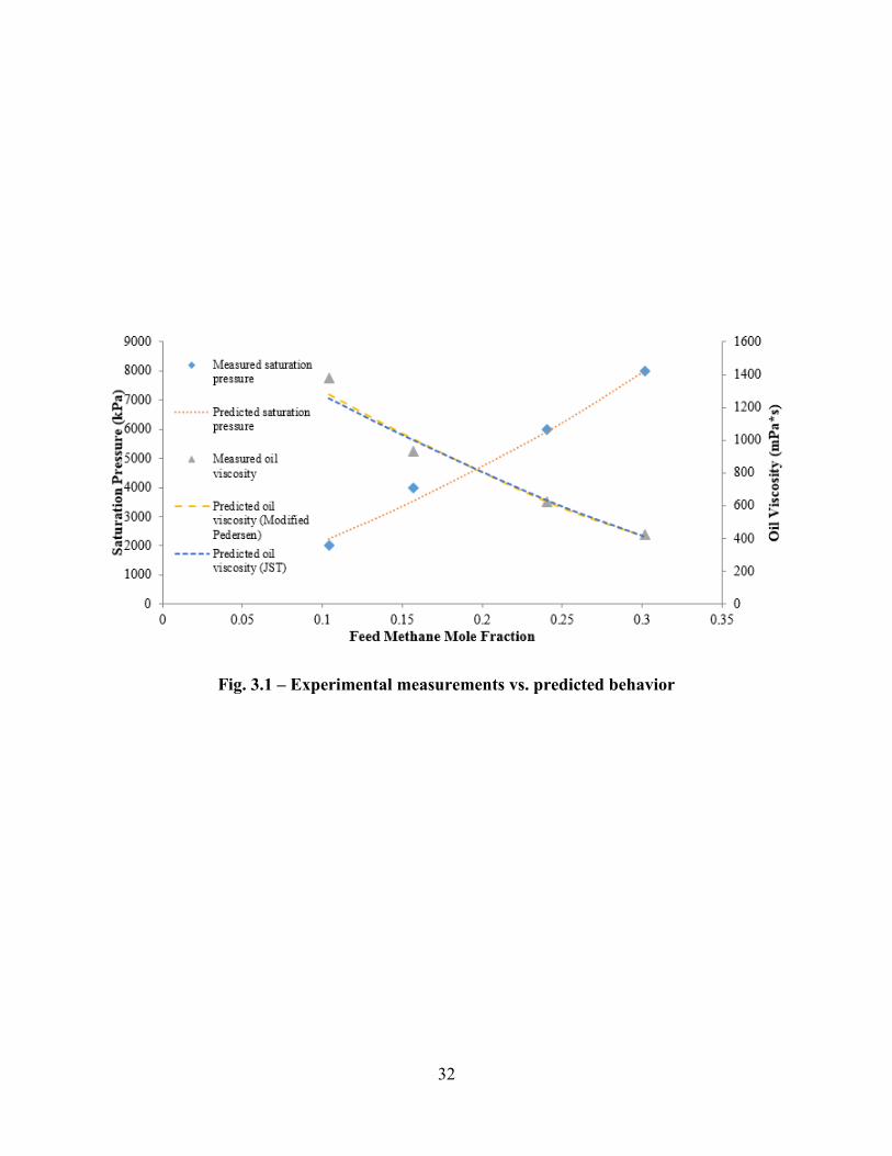
3.2 Fluid Model

Phase behavior is modeled based on the fluid composition analysis of a typical Canadian heavy

oil sample presented in Yadali Jamaloei (2013). The detailed fluid composition measured at the

Saskatchewan Research Council (SRC) is presented in Table 3.1. The Peng-Robinson Equation

of State (EOS) is used to model the experimental behavior of the fluid, which requires certain

parameters such as critical pressure, critical temperature, and acentric factor to be tuned via

regression analysis to match PVT experimental observations (i.e., saturation pressure and

viscosity profile). The experimental measurements are presented in Table 3.2 and Fig. 3.1

29

illustrates the experimental and predicted behavior of saturation pressure and viscosity after

tuning the equation of state.

Component lumping is implemented in order to reduce the number of calculations to be

performed by the compositional simulator. The lumping scheme and the resulting tuned critical

properties and acentric factors are presented in Table 3.3.

Flash calculations of methane-propane and dead oil mixtures are performed and the

corresponding predictions are compared with those presented in Yadali Jamaloei (2013) as a way

to validate the numerical PVT model and approximate the behavior of the mixtures in a gas

solvent injection scheme.

30

Table 3.1 – Fluid composition analysis

[Adapted from Yadali Jamaloei (2013)]

Component Mole % Component Mole %

C1 0.00

C23 2.11

C2 0.00

C24 1.82

C3 0.00

C25 1.91

IC4 0.30

C26 1.67

NC4 0.50

C27 1.65

IC5 1.25

C28 1.53

NC5 0.89

C29 1.44

C6 1.58

C30 1.30

C7 0.00

C31 1.24

C8 0.00

C32 1.27

C9 2.99

C33 0.87

C10 4.71

C34 0.89

C11 4.04

C35 1.13

C12 4.24

C36 1.08

C13 4.66

C37 0.69

C14 4.25

C38 0.71

C15 4.49

C39 1.16

C16 3.69

C40 1.12

C17 3.54

C41 0.61

C18 3.60

C42 0.58

C19 3.03

C43 1.02

C20 2.68

C44 0.65

C21 2.84

C45 0.63

C22 1.86 C46+ 17.78

31

Table 3.2 – Experimental measurements

[Adapted from Yadali Jamaloei (2013)]

Feed Methane Mole Fraction Saturation Pressure (kPa) Oil Viscosity (mPa*s)

0.1040 2,000 1,380

0.1566 4,000 930

0.2402 6,000 622

0.3018 8,000 424

Table 3.3 – Fluid properties after component lumping and regression

Component Molar Fraction Pc (atm) Tc (K) Acentric Factor

CH4 0.000 45.400 190.600 0.008

C3H8 0.000 41.900 369.800 0.152

IC4-C14 0.296 23.769 633.436 0.465

C15-C30 0.394 14.089 676.470 0.837

C31-C45+ 0.310 6.236 871.310 1.363

32

Fig. 3.1 – Experimental measurements vs. predicted behavior

33

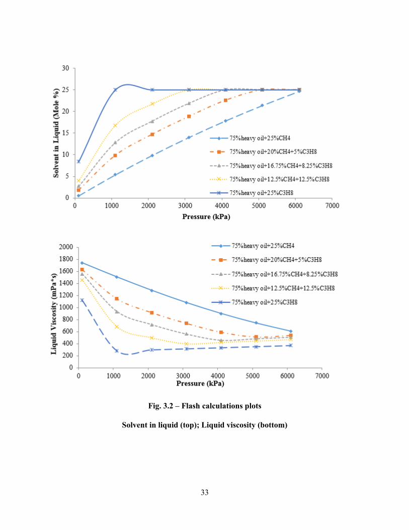
Fig. 3.2 – Flash calculations plots

Solvent in liquid (top); Liquid viscosity (bottom)

34

Live oil condition is approximated by injecting a mixture of methane and propane in

equal molar fractions (i.e., 50% C1 and 50% C3) until a typical field producing gas-oil ratio

(GOR) of 15 sm3/m3 is achieved. The live oil properties of the recombined sample (dead oil +

gas) is presented in Table 3.4.

Solvent injection processes typically use carbon dioxide (CO2) or a mixture of light

hydrocarbons components (e.g., methane, ethane, and propane). The molar composition of the

solvent mixture used for this study is 60% of methane and 40% of propane. This optimal

methane/propane ratio is highly dependent on the in-situ heavy oil properties; therefore, a

sensitivity analysis is recommended in order to find the optimal combination that renders the best

recovery response.

Table 3.4 – Live oil fluid properties after recombination

Component Molar Fraction Pc (atm) Tc (K) Acentric Factor

CH4 0.1153 45.400 190.600 0.008

C3H8 0.1153 41.900 369.800 0.152

IC4-C14 0.2278 23.769 633.436 0.465

C15-C30 0.3034 14.089 676.470 0.837

C31-C45+ 0.2382 6.236 871.310 1.363

35

Fig. 3.3 – Oil recovery for different combinations of methane-propane

3.2.1 Foamy Oil Model

The modified fractional-flow approach is adopted to represent the enhanced oil flow and delay of

free gas flow due to foamy oil behavior. This is achieved by assigning a lower gas relative

permeability end point, which is accompanied by higher irreducible gas saturation, during the

production stage. The relative permeability functions for the matrix and wormhole during the

injection/soaking stages are presented in Fig. 3.4, while the modified relative permeability

functions for the matrix and wormhole during the production stage are illustrated in Fig. 3.5.

Note the higher irreducible gas saturation and the lower end point of the gas function.

36

Fig. 3.4 – Relative permeability functions for injection and soaking

37

Fig. 3.5 – Relative permeability functions for production

3.3 Fine-Scale Models

A series of fine-scale three-dimensional compositional models in the Cartesian coordinates are

constructed. The model consists of 120 × 120 × 5 grid blocks (Δx = 0.25 m; Δy = 0.25 m). The

dimensions of the entire model are 30-meter wide, 30-meter long, and 1-meter thick. It is

assumed that the wormhole network is confined in the middle layer; therefore, Δz = 0.25 m in

the middle layer. The grid size along the z-direction in the over/underlying layers is computed

according to Eq. 3.1, which represents a logarithmic thickness refinement:

38

WH

HALFWHi

T

T

N

iTT

2ln

1

2exp

2 Eq. (3.1)

Where TWH denotes the thickness of the wormhole plane, i is the index of any individual

layer, N is the total number of layers, THALF is the half of the entire thickness, Ti is then the

distance from the outer boundary of layer i to the center of the wormhole plane.

Logarithmic thickness refinement is especially useful for improving the stability of the

numerical solution when high size contrast between adjacent grid blocks is present. The resulting

thickness corresponding to each layer is summarized in Table 3.5.

Table 3.5 – Thickness of each layer computed using logarithmic refinement

Layer Thickness (m)

1st 0.2386

2nd 0.1364

3rd (Wormhole) 0.2500

4th 0.1364

5th 0.2386

Due to the uncertainty in the actual wormhole configuration, a deterministic modeling of

the wormhole network is nearly impossible due to the unknown subsurface distribution of these

complex structures and the difficulty in gathering reliable data (e.g., seismic methods) to

39

delineate their precise configurations. Statistical approaches may offer a viable alternative to

characterize the wormhole networks. Following the diffusion-limited aggregation (DLA)

algorithm (Liu and Zhao, 2005), a series of fractal patterns representing networks of wormholes

extending in a 30 meters by 30 meters two-dimensional space is constructed. The fractal pattern

grows around the wellbore, which happens to be the geometrical center of the model. The sizes

of these network branches should closely approximate typical experimental and field

observations; for instance, the wormhole diameter is larger in near-wellbore region, and it

gradually decreases towards the tip of each branch).

These multiple realizations of two-dimensional fractal patterns are represented in a binary

form. Each fractal pattern is then converted to a wormhole network: blocks with a value of 1

belong to the wormhole network, and blocks with a value of 0 represent matrix [Fig. 3.6 (a)]. A

top view of the middle layer that contains the wormhole network, as well as the side view of the

model, are shown in Fig. 3.7 (a) and (b), respectively. Considering the spatial aggregation of

wormhole blocks, a range of wormhole diameter between 25 cm to 50 cm is obtained, which is

consistent with field observations in Chang and Ivory (2013).

Porosity and permeability for the matrix are derived from averages of several UCSS

reservoirs in Saskatchewan. Higher porosity and permeability values are assigned to the

wormhole blocks. Table 3.6 summarizes the main model attributes. In this study, additional sub-

grid heterogeneities in the matrix are not considered; therefore, dispersivity is set to zero in the

fine-scale model.

40

Fig. 3.6 – Binary representation and characterization of wormhole networks

(a) Binary system; (b) Number of wormholes in each coarse-scale grid block; (c) Wormhole

intensity in each coarse-scale grid block

Fig. 3.7 – Fine-scale model

(a) Side view of the model; (b) Wormhole layer

41

Table 3.6 – Model attributes

Parameter Units Value

Depth m 750

Thickness m 1

Reservoir Pressure MPa 2

Reservoir Temperature Celsius 20

Wormhole Porosity Fraction 0.60

Matrix Porosity Fraction 0.30

Wormhole Permeability Darcy 60

Matrix Permeability Darcy 3

Operating Conditions Units Value

Injection Composition

CH4 mol/mol 0.60

C3H8 mol/mol 0.40

Diffusion Coefficient cm2/s 0.001

Production Schedule Units Value

Injection Rate m3/day 25

Injection Time Day 20

Soaking Time Day 10

Production Pressure (BHP) MPa 1

42

The model is initialized to approximate the conditions commonly encountered at the end

of a typical CHOPS operation. Assuming a typical recovery factor of approximately 12% at the

end of CHOPS (Soh, 2016), the fluid saturations are then explicitly assigned in such a way that

the oil saturation in the matrix would gradually decrease with proximity to the depleted

wormholes (typically referred to as the depletion envelop). Fig. 3.8 illustrates the initial oil

saturation distribution (end of CHOPS) corresponding to one of the realizations for post-CHOPS

modeling. An initial pressure of 1,000–2,000 kPa is commonly observed in the field at the end of

CHOPS operation (Chang and Ivory, 2013).

Fig. 3.8 – Typical oil saturation distribution at the end of CHOPS

43

Operational constraints, such as solvent injection rate, type of solvent, and duration

corresponding to each one of the three stages in a typical cyclic solvent injection process are

scaled down from field practices to the model scale (Rangriz-Shokri, 2015). For instance, for the

injection stage, the injection rate is adjusted such that the total pore volume injected is

comparable to values reported in field/pilot applications; common practice usually entails an

injection period that continuously spans over 20 days, which is followed by 10 days of soaking

period. Finally, the well is brought on production by slowing decreasing the bottomhole pressure

(a 30-100 kPa/day depletion scheme is commonly used in the field). The terms “fine-scale

model” and “wormhole case” will be used interchangeably.

3.4 Coarse-Scale Models

A dual-permeability approach is employed to facilitate the scale-up process. Two systems are

defined in this approach: matrix and fracture systems, with the latter representing the wormhole

network. Different from the conventional dual-porosity system, a dual-permeability approach

allows flow between adjacent matrix blocks. Fig. 3.9 presents a graphical comparison between

the dual-porosity and dual permeability systems. Although the dual-permeability approach is

more expensive in terms of computational effort, it provides a more realistic approach to

modeling the actual interactions between the injected solvent and the in-situ heavy oil in the

matrix. The terms “coarse-scale model” and “dual-permeability case” will be used

interchangeably.

44

Fig. 3.9 – Illustration of flows in Dual-Porosity and Dual-Permeability systems

Corresponding to each fine-scale model generated in section 3.3, an equivalent coarse-

scale three-dimensional compositional model is constructed. The model consists of 24 × 24 × 1

grid blocks (Δx = 1.25 m; Δy = 1.25 m; Δz = 1 m). The dimensions of the entire model are 30-

meter wide, 30-meter long, and 1-meter thick (same as the fine-scale model). Each grid block in

the coarse-scale model is the equivalence of 75 fine-scale grid blocks. The dimensions of the

coarse blocks are Δx = 1.25 m, Δy = 1.25 m, and Δz = 1 m respectively. Fig. 3.10 illustrates a

comparison of fine-scale and coarse-scale grid blocks.

45

Fig. 3.10 – Fine-scale vs. coarse-scale

Fracture and matrix porosities in the coarse-scale (dual-permeability) model, ØF(DK) and

ØM(DK), are computed via volume-weighted linear averaging using Eq. 3.2 and Eq. 3.3,

respectively:

coarse

WHWHDKF

V

V )(

Eq. (3.2)

coarse

MMDKM

V

V )(

Eq. (3.3)

Where Vcoarse denotes the bulk volume of the coarse-scale block; V and Ø denote volume

and porosity, respectively, while the subscripts “WH” and “M” denote wormhole and matrix

properties, respectively. The shape factor (σ) is another parameter required to fully describe dual-

permeability systems. It is needed to compute the fluid transfer between the matrix and the

46

fracture systems. According to the formulation introduced by Gilman and Kazemi (1983), as

presented in Eq. 3.4:

222

1114

zyx LLL Eq. (3.4)

Where Lx, Ly, and Lz denote the fracture spacing along the x-, y-, and z- direction,

respectively. Given that shape factor is multiplied with the interfacial area of a given grid block

to represent the total contact area between the matrix and fracture systems, it is calculated based

on the actual contact area between all the matrix and the wormhole cells in the fine-scale model

for each coarse-scale grid block. A uniform fracture spacing (Lx = Ly = Lz) is chosen in such a

way that they would reproduce the same matrix-wormhole contact area as in the fine-scale

model.

Finally, to compute the bivariate relationships between wormhole intensity (WI) and

effective dispersivities for the dual-permeability system, a flow-based technique is adopted. First,

WI is computed for each coarse-scale grid block: WI = VWH/Vcoarse [Fig. 3.6 (c)]. Since WI

would vary spatially (e.g., WI decreases away from the well), three bins of WI values are

considered: high wormhole intensity (WI ≥ 60%), medium wormhole intensity (30% < WI <

60%), and low wormhole intensity (WI ≤ 30%). An objective function, in terms of mismatch in

the cumulative oil and gas production profiles between the fine-scale model and the equivalent

coarse dual-permeability system, is defined. Longitudinal and transverse dispersivities (αL and

αT) in both the fracture and matrix systems, corresponding to each bin, are tuned to minimize the

47

mismatch. This step is implemented using CMG’s C-MOST (CMG-CMOST, 2016) for all fine-

scale models constructed in sections 3.3 and 3.4.

Multiple random realizations of the wormhole networks (30 m × 30 m) generated with

the diffusion-limited aggregation (DLA) algorithm are illustrated in Fig. 3.11. All these

wormhole networks have similar overall areal coverage, which is approximately 12% of the

entire layer in which each network is explicitly modeled (this corresponds to a 2.3% volumetric

coverage over the entire pay thickness, as reported in most field operations).

48

Fig. 3.11 – Multiple wormhole networks used for calibration

49

In the end, distributions of effective dispersivities corresponding to different categories of

wormhole intensity, i.e., P(αL,i|WI) and P(αT,i|WI), are constructed (i = matrix, fracture). This

step is facilitated by fitting a distinctive Gaussian function corresponding to the set of effective

dispersivity values in each bin. The entire scale-up workflow is summarized in Fig. 3.12. The

calibrated bivariate distributions are used in a cloud transform procedure to construct models of

αL and αT, which are correlated to WI (wormhole intensity), at the field scale (considering a grid

size that is the same as the coarse block). This means assigning effective dispersivities at each

location by sampling from P(αL,i|WI) and P(αT,i|WI) according to the WI value/bin at that

particular location (Vishal and Leung, 2015). In this study, values are sampled from the series of

Gaussian functions obtained from the aforementioned scale-up analysis.

Fig. 3.12 – Summary of the scale-up workflow

As an example, 7 realizations of the fine-scale models are constructed, and the coarse-

scale dispersivity values for both fracture and matrix systems corresponding to each WI level are

summarized in Table 3.7. These values are also plotted in Fig. 3.13 and Fig. 3.14. It is observed

that as wormhole intensity increases, fracture dispersivity also increases. This reflects the

additional mixing as a result of variation in flow paths among the wormholes. On the other hand,

50

as wormhole intensity increases, the contribution to solvent transport from matrix dispersion is

less prominent, since less matrix volume is remaining in a bulk grid block. Therefore, a

decreasing trend in matrix dispersivity with wormhole intensity is observed. Fig. 3.15 shows the

fitted Gaussian distributions of effective dispersivity in the fracture and matrix systems for

different levels of wormhole intensity (WI). Fig. 3.16 illustrates the cumulative distribution

functions (CDF) of the Gaussian bivariate distributions respectively.

Table 3.7 – History-matched dispersivities for the matrix and fracture systems

Wormhole Intensity

High

60-100%

Medium

30-60%

Low

0-30%

Case A Fracture 4.8875 3.1500 0.9525

Matrix 0.9725 2.6100 5.5000

Case B Fracture 4.2000 1.5050 0.9850

Matrix 0.7725 1.6650 3.6900

Case C Fracture 4.3500 1.9450 1.0500

Matrix 1.1850 1.5500 3.5300

Case D Fracture 4.1700 2.1000 0.8275

Matrix 0.8050 2.3700 3.9600

Case E Fracture 3.8500 1.6650 0.8375

Matrix 0.9900 1.8800 3.4500

Case F Fracture 3.2000 2.5000 0.8000

Matrix 0.8000 2.3000 3.4000

Case G Fracture 4.8200 2.2350 0.8750

Matrix 0.9200 2.1800 4.7700

51

Fig. 3.13 – Bivariate distribution of WI and Dispersivity (αL = αT) in the Fracture

Fig. 3.14 – Bivariate distribution of WI and Dispersivity (αL = αT) in the Matrix

52

Fig. 3.15 – Fitted Gaussian distributions of dispersivity

Fracture System (top); Matrix System (bottom)

53

Fig. 3.16 – Cumulative distribution functions (CDFs)

Fracture System (top); Matrix System (bottom)

54

Chapter 4: Validation

4.1 Fine-Scale Model

Consider a field-scale model of 75-meter wide, 75-meter long, and 1-meter thick. For

comparative purposes, models at two different resolutions are used. First, a high-resolution

model is constructed, such that the complex wormhole pattern is explicitly represented in the

computational domain. The model, as shown in Fig. 4.1, is 60 × 60 × 3 (∆x = 1.25 m; ∆y = 1.25

m; ∆z = 0.375, 0.25, and 0.375 m, respectively). The blocks containing the wormholes are

locally refined (∆x = 0.25 m; ∆y = 0.25 m; ∆z = 0.25 m). The complex wormhole network

extends in the middle layer. The initial conditions are the same as those presented in section 3.3.

To mimic realistic field operating conditions, an injection period of 20 days, followed by 10 days

of soaking, is modeled. The injection rate is modified from the calibration models in sections 3.3

and 3.4, in order to maintain the same injected pore volume.

55

Fig. 4.1 – Fine-scale model

4.2 Coarse-Scale Model

Next, an equivalent dual-permeability continuum is constructed following the procedure

described in section 3.4 as presented in Fig. 4.2. A total of 25 realizations of dispersivity values

(fracture and matrix systems) are sampled, and their cumulative oil and gas production profiles

are compared with the high-resolution model in Fig. 4.3.

56

Fig. 4.2 – Coarse-scale model

57

Fig. 4.3 – Cumulative oil production for the field-scale model

High-resolution model (blue); Coarse model with average properties (green); Coarse model

with zero dispersivity (red); Coarse models following the proposed scale-up workflow

(other colors)

58

Fig. 4.4 – Cumulative gas production for the field-scale model

High-resolution model (blue); Coarse model with average properties (green); Coarse model

with zero dispersivity (red); Coarse models following the proposed scale-up workflow

(other colors)

59

Also shown in Fig. 4.3 and Fig. 4.4 are two additional cases of coarse models:

Green curve: constant WI of 45% (corresponding to a fracture spacing of 0.65 m) is

assigned everywhere. This choice is based on an average WI value within a 12.5 m radius around

the wellbore in the high-resolution model. The set-up depicts a scenario where the WI observed

in the near wellbore region is mistakenly used to populate the entire model. Corresponding

average dispersivity values of 4.21 m and 0.92 m are sampled from Fig. 3.13 for the fracture and

matrix systems, respectively.

Red curve: constant WI of 72% (corresponding to a fracture spacing of 0.3 m) is assigned

everywhere. Dispersivity is set to zero (same as the high-resolution model) everywhere.

Fig. 4.5 illustrates the solvent distribution at the end of the injection period for both the fine-scale

and coarse-scale model, and Fig. 4.6 shows the oil saturation of the end of the production period.

Fig. 4.5 – Solvent distribution at the end of injection period

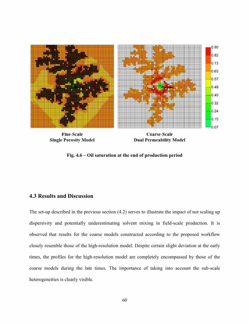
60

Fig. 4.6 – Oil saturation at the end of production period

4.3 Results and Discussion

The set-up described in the previous section (4.2) serves to illustrate the impact of not scaling up

dispersivity and potentially underestimating solvent mixing in field-scale production. It is

observed that results for the coarse models constructed according to the proposed workflow

closely resemble those of the high-resolution model. Despite certain slight deviation at the early

times, the profiles for the high-resolution model are completely encompassed by those of the

coarse models during the late times. The importance of taking into account the sub-scale

heterogeneities is clearly visible.

61

One of the main challenges in reservoir simulation is achieving a balance between

accuracy and computational cost. This practical approach, involving a dual-permeability model,

can offer the opportunity to reduce computational effort drastically as shown in Fig. 4.5. Reliable

and efficient field-scale simulations with multiple well patterns can be performed by accounting

for the contribution of sub-scale heterogeneities (wormhole configurations) in the transport and

mixing of solvent and heavy oil in post-CHOPS applications.

Fig. 4.7 – Reduction in computational time

62

Chapter 5: Design of Field-Scale Applications

This chapter focuses on the application of the proposed workflow to scale up solvent transport

mechanisms in wormhole networks at a larger scale. The implementation of this workflow

reduces the computational time significantly, which permits the proper assessment of multiple

strategies to increase the recovery factor from post-CHOPS reservoirs by carrying out sensitivity

analyses; several factors such as injection parameters, soaking time, and number of cycles are

examined.

5.1 Injection Scheme

The main cost associated with most solvent-aided EOR applications is typically that of the

solvent mixture. Provided that the solvent cost is highly dependent on the fluctuating market, the

solvent volume available for injection could be identified as the key constraint for any potential

application. A careful PVT study is always recommended in order to properly select the optimal

solvent mixture for a particular heavy oil composition.

Once the solvent combination has been determined, the associated costs and its

availability in field locations can be taken into account during the economic assessment of the

project. The common approach in field operations is to keep injecting the selected solvent

mixture until the reservoir pressure has returned to its initial value approximately (Chang and

Ivory, 2013). Although this would be the ideal scenario, it is not always feasible due to the

difficulty in maintaining an increasing trend in reservoir pressure, particularly when other nearby

63

wells are on production. Nevertheless, a proper injection scheme should aim to achieve partial

miscibility between the solvent and heavy oil at the downhole pressures. For the field-scale

model under consideration (75 m x 75 m x 3.5 m), the cumulative solvent injection profile is

presented in Fig. 5.1. As discussed in section 3.2, the model is initially depleted to mimic the

conditions and fluid distribution at the end of CHOPS. This pressure depletion process takes

about six months with surface oil rates decreasing from 30 to 2 sm3/day, where the final

bottomhole pressure of 1,690 kPa is reached. A cut-off value of of 2 sm3/day is set for the

surface oil rate, as it is value commonly-adopted at most CHOPS wells (Dusseault, 2007).

In this case, the proposed injection scheme increases the average reservoir pressure from

1,690 kPa to its initial level (4,000 kPa), as illustrated in the pressure profile in Fig. 5.2. Once the

desired reservoir pressure has been reached, solvent injection is stopped and the well is shut-in.

64

Fig. 5.1 – Cumulative solvent injection profile

Fig. 5.2 – Average reservoir pressure profile

65

5.2 Optimal Soaking Time

As explained in previously, in most of the cases, the soaking duration is often arbitrarily selected

or adopted from analog wells or previous applications. As a general rule of thumb, the soaking

time should be at least half of the injection time, as evidenced in the pilot field applications

(Husky Energy, 2011).

It would be reasonable to expect that longer soaking periods render a better recovery

response. It is true that prolonged soaking times may increase the amount of heavy oil effectively

contacted by the solvent, which would ultimately increase the final recovery factor. This

postulation is supported by the following analysis, where different soaking times are examined,

and the total recovery factors after a fixed production period of 190 days are presented in Table

5.1.

Table 5.1 – Recovery factor for different soaking times

Soaking Time (day) Recovery Factor

10 9.24%

15 9.26%

18 9.26%

20 9.54%

22 9.54%

25 9.74%

30 10.01%

66

Fig. 5.3 – Oil surface rates for different soaking times

In addition, differences in decline profiles at early and late times corresponding to

different soaking periods are also noted. For longer soaking periods, a slower decline at late

times is identified; however, lower rate at early times is also observed. This difference is better

illustrated by comparing the production profiles corresponding to two different soaking periods

(22 days vs. 30 days) in Fig. 5.3. Comparing the saturation maps of these two cases (Fig. 5.4),

the area that is effectively drained at the end of the production phase exhibit roughly the same

67

areal extent. By examining the corresponding solvent distribution in the wormhole networks in

Fig. 5.5, it is evident that the solvent has effectively mobilized much of the oil from the drainage

area after 22 days of soaking, reducing the oil viscosity and initiating additional solution-gas

drive. However, as the soaking period continues to 30 days, the solvent has reached regions that

are beyond the drainage area, diluting the solvent concentration in the near-well area, which

contributes to the reduced initial oil production. Recovery of additional oil from regions that are

far away would only contribute to the late-time production, when the rate has already declined

considerably.

This difference of decline characteristics precisely explains why the 22-day case is the

optimal one, if an economic limit of 2 sm3/day, which represents the typical (post-) CHOPS

constraint in Western Canada (Dusseault, 2007), is imposed. According to the results in Table

5.2, the optimal soaking time corresponding to the highest recovery factor up to the economic

limit, is found to be 22 days. Comparing the 22-day and 30-day cases, it takes essentially the

same number of producing days to reach the economic limit (115 days and 114 days for the 22-

day and 30-day soaking periods, respectively).

The results support the conclusion that the economic limit would play an important role

in determining the optimal soaking period. If the economic limit is zero, soaking the reservoir for

extended periods of time would be ideal. In the end, the optimal condition depends on the trade-

off between extracting additional oil recovery at late times versus producing at a higher rate at

early times.

68

Table 5.2 – Recovery factor for different soaking times when an economic limit is enforced

Soaking Time (day) Recovery Factor

10 6.83%

15 6.81%

18 6.45%

20 6.86%

22 7.21%

25 6.85%

30 6.85%

Fig. 5.4 – Oil saturation map after different soaking periods

69

Fig. 5.5 – Global propane (solvent) distribution after different soaking periods

In the particular scenario that a lower oil production is not a constraint, soaking the

reservoir for extended periods of time turns out to be more beneficial than shorter periods.

Provided that time is not constraint, prolonged times increase the effective drainage area, which

can be contacted by the solvent if long soaking periods are allowed, therefore mobilizing heavy

oil from even further regions.

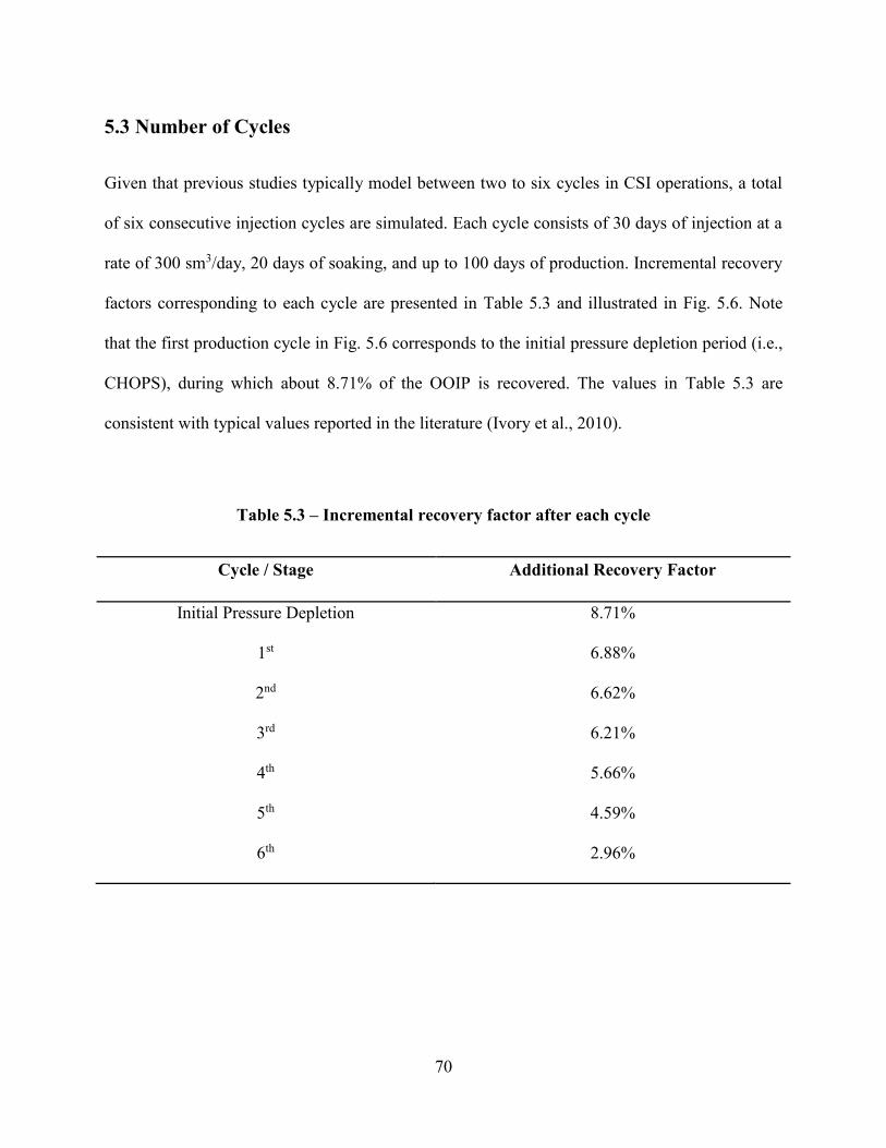
70

5.3 Number of Cycles

Given that previous studies typically model between two to six cycles in CSI operations, a total

of six consecutive injection cycles are simulated. Each cycle consists of 30 days of injection at a

rate of 300 sm3/day, 20 days of soaking, and up to 100 days of production. Incremental recovery

factors corresponding to each cycle are presented in Table 5.3 and illustrated in Fig. 5.6. Note

that the first production cycle in Fig. 5.6 corresponds to the initial pressure depletion period (i.e.,

CHOPS), during which about 8.71% of the OOIP is recovered. The values in Table 5.3 are

consistent with typical values reported in the literature (Ivory et al., 2010).

Table 5.3 – Incremental recovery factor after each cycle

Cycle / Stage Additional Recovery Factor

Initial Pressure Depletion 8.71%

1st 6.88%

2nd 6.62%

3rd 6.21%

4th 5.66%

5th 4.59%

6th 2.96%

71

Fig. 5.6 – Cumulative recovery factor for six cycles

As expected, a decreasing trend in the incremental recovery factor with increasing cycle

is observed (Fig. 5.7). The two initial cycles contribute most significantly to the overall oil

recovery. If an economic rate in the range of 2 to 3 sm3/day (16.8 to 25.2 bbl/day) is defined, the

number of producing days would also exhibits a decreasing trend as evidenced in Fig. 5.8.

Therefore, it is hypothesized that it would be more beneficial to implement fewer and longer

cycles than more shorter cycles. This aspect will be explored further in the next section.

72

Fig. 5.7 – Incremental recovery factor after each cycle

Fig. 5.8 – Surface oil rate in each cycle

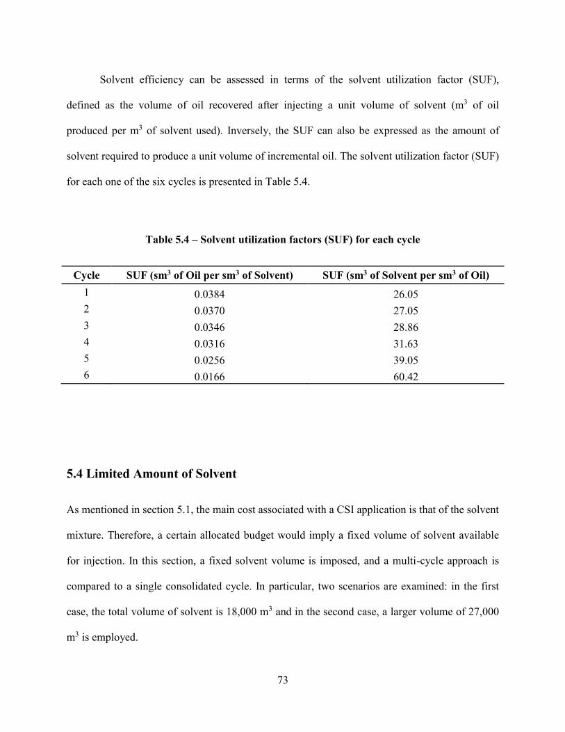
73

Solvent efficiency can be assessed in terms of the solvent utilization factor (SUF),

defined as the volume of oil recovered after injecting a unit volume of solvent (m3 of oil

produced per m3 of solvent used). Inversely, the SUF can also be expressed as the amount of

solvent required to produce a unit volume of incremental oil. The solvent utilization factor (SUF)

for each one of the six cycles is presented in Table 5.4.

Table 5.4 – Solvent utilization factors (SUF) for each cycle

Cycle SUF (sm3 of Oil per sm3 of Solvent) SUF (sm3 of Solvent per sm3 of Oil)

1 0.0384 26.05

2 0.0370 27.05

3 0.0346 28.86

4 0.0316 31.63

5 0.0256 39.05

6 0.0166 60.42

5.4 Limited Amount of Solvent

As mentioned in section 5.1, the main cost associated with a CSI application is that of the solvent

mixture. Therefore, a certain allocated budget would imply a fixed volume of solvent available

for injection. In this section, a fixed solvent volume is imposed, and a multi-cycle approach is

compared to a single consolidated cycle. In particular, two scenarios are examined: in the first

case, the total volume of solvent is 18,000 m3 and in the second case, a larger volume of 27,000

m3 is employed.

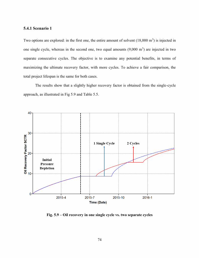
74

5.4.1 Scenario 1

Two options are explored: in the first one, the entire amount of solvent (18,000 m3) is injected in

one single cycle, whereas in the second one, two equal amounts (9,000 m3) are injected in two

separate consecutive cycles. The objective is to examine any potential benefits, in terms of

maximizing the ultimate recovery factor, with more cycles. To achieve a fair comparison, the

total project lifespan is the same for both cases.

The results show that a slightly higher recovery factor is obtained from the single-cycle

approach, as illustrated in Fig 5.9 and Table 5.5.

Fig. 5.9 – Oil recovery in one single cycle vs. two separate cycles

75

Table 5.5 – Recovery factor for Scenario 1

Type Recovery Factor

2 Separate Cycles

1st: 15.58%

2nd: 7.11%

Total: 22.19%

1 Combined Cycle 22.70%

5.4.2 Scenario 2

Once again, multi-cycle and single-cycle strategies are compared. Two options are explored: in

the first one, the entire amount of solvent (27,000 m3) is injected in one single cycle; in the

second, three equal amounts (9,000 m3) are injected in three separate consecutive cycles. Same

observation as in 5.4.1 is noted: a slightly higher recovery factor is obtained from the first

approach as illustrated in Fig. 5.10 and Table 5.6.

The results from these two scenarios appear to support the hypothesis that it would be

more beneficial to implement fewer, longer cycles than multiple shorter cycles. Provided that the

amount of solvent is fixed, it is then concluded that implementing one single cycle is likely to be

more effective, in terms of recovery factor, than a series of shorter (injection-soaking-

production) consecutive cycles.

Incorporating the findings from section 5.2, it is proposed that injecting larger volumes of

solvent and extending the soaking times are recommended during the first and/or second cycles.

In addition, when the amount of solvent available is limited, it would be more effective to inject

76

all the solvent in one single consolidated cycle, possibly with an extended soaking period, rather

than performing shorter consecutive cycles.

Fig. 5.10 – Oil recovery in one single cycle vs. three separate cycles

77

Table 5.6 – Recovery factor for Scenario 2

Type Recovery Factor

3 Separate Cycles

1st: 15.58%

2nd: 7.11%

3rd: 5.68%

Total: 28.37%

1 Combined Cycle 29.61%

78

Chapter 6: Conclusions and Recommendations for Future Work

6.1 Conclusions

This work presented a workflow to assign effective parameters in a dual-permeability continuum

model for modeling post-CHOPS CSI processes. Variables including matrix/fracture porosity,

fracture spacing, shape factors, and longitudinal/transverse dispersivities are computed in

accordance with the fine-scale wormhole characteristics within a coarse-scale grid block. The

calculation procedure is repeated over multiple realizations of wormhole configurations,

allowing bivariate distributions of effective longitudinal/transverse dispersivities to be calibrated

as functions of wormhole intensity. The calibrated distributions are used in a cloud transform

procedure to construct models of effective dispersivities for field-scale simulations.

In contrast to many existing numerical analysis approaches that involve arbitrary

adjustment of dispersivity via history matching, the developed workflow offers a novel and

systematic framework to scale up solvent dispersivity in post-CHOPS applications. Fracture

spacing, shape factor and dispersivity are assigned in a fashion that honors the realistic spatial

variation in wormhole characteristics at the fine scale.

A synthetic case study involving typical petrophysical values and operational parameters

for post-CHOPS reservoirs is presented. Shape factors and effective dispersivity values in the

dual-permeability coarse models are assigned following the proposed workflow. In addition to >

90% reduction in computational time, results for the coarse models closely resemble those of the

79

high-resolution model. Except for some slight deviation during early times, the profiles for the

high-resolution model are completely encompassed by those of the coarse models during the late

times. The outcomes highlight the importance of properly capturing sub-scale heterogeneity

effects during scale-up. The model is used to evaluate multiple production scenarios to assess the

impacts of number and duration of CSI cycles on production efficiency.

Though previous numerical studies have examined the optimization of CSI processes, a

lack of proper scale-up procedures has rendered their description of heterogeneous wormhole

networks at the field scale incomplete, which could potentially compromise the reliability of the

corresponding optimization results. It is argued that the model employed in this study could

better represent the detailed wormhole features at the coarse scale; hence, it is more appropriate

for field-scale operations design. The aforementioned scale-up procedure was implemented to

construct coarse-scale simulation models to provide insights on operational strategies and key

considerations when optimizing cyclic solvent injection (CSI) processes in field-scale

applications:

Extended soaking period could positively impact the ultimate oil recovery, but it also

inadvertently lowers the early production. The optimal soaking period is a function of the

economic limit, as it reflects a trade-off between extracting additional oil recovery at late

times versus producing at a higher rate at early times.

The results support the hypothesis that it is more effective to implement fewer, but

longer, cycles instead of more, yet shorter, cycles. In particular, if the amount of solvent

is limited, it would be more effective to inject all the solvent in one single consolidated

cycle, possibly with an extended soaking period, rather than performing shorter

80

consecutive cycles. Generally speaking, it is recommended to inject larger volumes of

solvent and extending the soaking times during the first and/or second cycles.

6.2 Future Work

This systematic workflow can be extended to incorporate other foamy-oil modeling approaches,

such as the kinetic and the pseudo-bubble point models, to assess the impact of pressure

depletion strategies on the non-equilibrium foamy oil behavior.

Future studies should focus on the application of this practical workflow to model

multiple production scenarios to assess the impacts of pressure depletion schedule in the solvent

transport and to study the interactions between wormhole characteristics and non-equilibrium

phase behavior (e.g., solution or dissolution of foamy oil; distribution of free gas during post-

CHOPS) at the field-scale using kinetic approaches.

81

Bibliography

Babadagli, T., & Rangriz-Shokri, A. (2013, June). Modeling Thermal and Solvent Injection

Techniques as Post-CHOPS Applications Considering Geomechanical and Compositional

Effects. Presented at the SPE Heavy Oil Conference-Canada held in Calgary, Canada June 11-

13. Society of Petroleum Engineers.

Bera, A., & Babadagli, T. (2016). Relative permeability of foamy oil for different types of

dissolved gases. SPE Reservoir Evaluation & Engineering, 19(04), 604-619.

Chang, J., & Ivory, J. (2013). Field-scale simulation of cyclic solvent injection (CSI). Journal of

Canadian Petroleum Technology, 52(04), 251-265.

Chang, J., & Ivory, J. (2015, June). History Match and Strategy Evaluation for CSI Pilot.

Presented at the SPE Canada Heavy Oil Technical Conference held in Calgary, Canada June 9-

11. Society of Petroleum Engineers.

Chang, J., Ivory, J., & London, M. (2015, June). History Matches and Interpretation of CHOPS

Performance for CSI Field Pilot. Presented at the SPE Canada Heavy Oil Technical Conference

held in Calgary, Canada June 9-11. Society of Petroleum Engineers.

82

Claridge, E. L. (1994). A Proposed Model and Mechanism for Anomalous Foamy Heavy Oil

Behavior. Presented at the International Heavy Oil Symposium held in Calgary, Canada June 19-

21. Society of Petroleum Engineers.

Computer Modelling Group Ltd. (2016). GEM Compositional & Unconventional Reservoir

Simulator - User Guide.

Computer Modelling Group Ltd. (2016). WinProp Phase-Behaviour & Fluid Property Program -

User Guide.

Denney, D. (1999). Wormhole-Network Model of Cold Production in Heavy Oil. Journal of

Petroleum Technology, 51(09), 102-104.

Du, Z., Zeng, F., & Chan, C. (2015). An experimental study of the post-CHOPS cyclic solvent

injection process. Journal of Energy Resources Technology, 137(4), 042901.

Fan, Z., & Yang, D. (2016, April). Characterization of Wormhole Growth and Its Applications

for CHOPS Wells Using History Matching. Presented at the SPE Improved Oil Recovery

Conference held in Tulsa, USA April 11-13. Society of Petroleum Engineers.

Fan, Z., & Yang, D. (2017, February). Quantification of Sand Production by Use of a Pressure-

Gradient-Based Sand Failure Criterion. Presented at the SPE Canada Heavy Oil Technical

Conference held in Calgary, Canada February 15-16. Society of Petroleum Engineers.

83

Fan, Z., Yang, D., & Li, X. (2017, May). Determination of Three-Phase Relative Permeability in

CHOPS Processes by Use of an Improved Iterative Ensemble Smoother. Presented at the SPE

Reservoir Characterization and Simulation Conference and Exhibition held in Abu Dhabi, UAE.

Society of Petroleum Engineers.

Firoozabadi, A. (2001). Mechanisms of solution gas drive in heavy oil reservoirs. Journal of

Canadian Petroleum Technology, 40(03), 15-20.

Haddad, A. S., & Gates, I. (2015). Modelling of Cold Heavy Oil Production with Sand (CHOPS)

using a fluidized sand algorithm. Fuel, 158, 937-947.

Husky Energy. (2011, November 30). Husky Oil’s Mervin Cold Solvent EOR Pilot Final

Technical Report for the SPRO Program. Saskatchewan Petroleum Research Incentive.

Istchenko, C. M., & Gates, I. D. (2014). Well/Wormhole model of cold heavy-oil production

with sand. SPE Journal, 19(02), 260-269.

Istchenko, C., & Gates, I. D. (2011, January). The well-wormhole model of cold production of

heavy oil reservoirs. Presented at the SPE Heavy Oil Conference and Exhibition held in Kuwait

City, Kuwait. Society of Petroleum Engineers.

Ivory, J., Chang, J., Coates, R., & Forshner, K. (2010). Investigation of cyclic solvent injection

process for heavy oil recovery. Journal of Canadian Petroleum Technology, 49(09), 22-33.

84

Jia, X., Li, J., Chen, Z., Gu, Y., & Zeng, F. (2016, May). Modeling of Foamy-Oil Flow in

Solvent-Based Recovery Processes. Presented at the SPE EUROPEC featured at 78th EAGE

Conference and Exhibition held in Vienna, Austria. Society of Petroleum Engineers.

Kraus, W. P., McCaffrey, W. J., & Boyd, G. W. (1993, January). Pseudo-bubble point model for

foamy oils. Presented at the Annual Technical Meeting held in Calgary, Canada. Petroleum

Society of Canada.

Lebel, J. P. (1994, March). Performance implications of various reservoir access geometries.

In 11th Annual Heavy Oil & Oil Sands Tech. Symp., March (Vol. 2).

Li, H., Zheng, S., & Yang, D. T. (2013). Enhanced swelling effect and viscosity reduction of

solvent (s)/CO2/heavy-oil systems. SPE Journal, 18(04), 695-707.

Li, X., Yin, Y., Yang, Z., Shen, Y., & Liu, Z. (2016, June). Produced Gas Reinjection Based

Cyclic Solvent Processes for Foamy Oil Reservoirs in the Eastern Orinoco Belt, Venezuela.

Presented at the SPE Canada Heavy Oil Technical Conference held in Calgary, Canada June 7-9.

Society of Petroleum Engineers.

Liu, X., & Zhao, G. (2005). A fractal wormhole model for cold heavy oil production. Journal of

Canadian Petroleum Technology, 44(09).

Maini, B. B. (2001). Foamy-oil flow. Journal of Petroleum Technology, 53(10), 54-64.

85

Martinez-Gamboa, J. J., Wang, M., & Leung, J. Y. (2017, May). A Practical Approach for Scale-

Up of Solvent Transport Mechanisms in Post-CHOPS EOR Applications. Presented at the SPE

Latin America and Caribbean Petroleum Engineering Conference held in Buenos Aires,

Argentina May 17-19. Society of Petroleum Engineers.

Naderi, K., & Babadagli, T. (2016). Solvent Selection Criteria and Optimal Application

Conditions for Heavy-Oil/Bitumen Recovery at Elevated Temperatures: A Review and

Comparative Analysis. Journal of Energy Resources Technology, 138(1), 012904.

Naderi, K., Romaniuk, N., & Ozum, B. (2015, October). Improvement of the CHOPS Process

Efficiency. Presented at the SPE Kuwait Oil and Gas Show and Conference held in Mishref,

Kuwait October 11-14. Society of Petroleum Engineers.

Pooladi-Darvish, M., & Firoozabadi, A. (1999). Solution-gas drive in heavy oil reservoirs.

Journal of Canadian Petroleum Technology, 38(04).

Rangriz-Shokri, A., & Babadagli, T. (2015). Field-Scale Deformation Analysis of Cyclic Solvent

Stimulation in Thin Unconsolidated Heavy-Oil Reservoirs with Developed Wormhole Network.

Journal of Canadian Petroleum Technology, 54(06), 341-350.

Rangriz-Shokri, A., & Babadagli, T. (2016). A Sensitivity Analysis of Cyclic Solvent

Stimulation for Post-CHOPS EOR: Application on an Actual Field Case. SPE Economics &

Management 8(04), 78-89.

86

Rangriz-Shokri, A. R., & Babadagli, T. (2014). Modelling of Cold Heavy-Oil Production with

Sand for Subsequent Thermal/Solvent Injection Applications. Journal of Canadian Petroleum

Technology, 53(2), 95-108.

Rangriz-Shokri, & Babadagli, T. (2016). Field scale modeling of CHOPS and solvent/thermal

based post CHOPS EOR applications considering non-equilibrium foamy oil behavior and

realistic representation of wormholes. Journal of Petroleum Science and Engineering, 137, 144-

156.

Sheng, J. J., Maini, B. B., Hayes, R. E., & Tortike, W. S. (1999). Critical review of foamy oil

flow. Transport in Porous Media, 35(2), 157-187.

Soh, Y. J., Rangriz-Shokri, A., & Babadagli, T. (2016, September). A New Modeling Approach

to Optimize Methane-Propane Injection in a Field after CHOPS. Presented at the SPE Annual

Technical Conference and Exhibition held in Dubai September 26-28. UAE. Society of

Petroleum Engineers.

Speight, J. G. (2013). Enhanced recovery methods for heavy oil and tar sands. Elsevier.

Sun, X., Dong, M., Zhang, Y., & Maini, B. B. (2015). Enhanced heavy oil recovery in thin

reservoirs using foamy oil-assisted methane huff-n-puff method. Fuel, 159, 962-973.

87

Tremblay, B., Sedgwick, G., & Forshner, K. (1996, January). Modelling of sand production from

wells on primary recovery. Presented at the Annual Technical Meeting held in Calgary, Canada.

Petroleum Society of Canada.

Tremblay, B., Sedgwick, G., & Forshner, K. (1997). Simulation of cold production in heavy-oil

reservoirs: wormhole dynamics. SPE Reservoir Engineering, 12(02), 110-117.

Vishal, V., & Leung, J. Y. (2015). Modeling impacts of subscale heterogeneities on dispersive

solute transport in subsurface systems. Journal of contaminant hydrology, 182, 63-77.

Yang, P., Li, H., & Yang, D. (2014). Determination of Saturation Pressures and Swelling Factors

of Solvent (s)–Heavy Oil Systems under Reservoir Conditions. Industrial & Engineering

Chemistry Research, 53(5), 1965-1972.

Yuan, J. Y., Tremblay, B., & Babchin, A. (1999). A wormhole network model of cold

production in heavy oil. Presented at the SPE International Thermal Operations and Heavy Oil

Symposium held in Bakersfield, USA March 17-19. Society of Petroleum Engineers.

Zhang, M., Du, Z., Zeng, F., Hong, S. Y., & Xu, S. (2016). Upscaling study of the cyclic solvent

injection process for post‐CHOPS reservoirs through numerical simulation. The Canadian

Journal of Chemical Engineering, 94(7), 1402-1412.