Scalable Performance Measurement and Analysis

Todd Gamblin

A dissertation submitted to the faculty of the University of North Carolina at Chapel Hill inpartial fulfillment of the requirements for the degree of Doctor of Philosophy in the Depart-ment of Computer Science.

Chapel Hill2009

Approved by:

Daniel A. Reed, Advisor

Robert J. Fowler, Reader

Bronis R. de Supinski, Reader

Jan F. Prins, Committee Member

Frank Mueller, Committee Member

c© 2009Todd Gamblin

ALL RIGHTS RESERVED

ii

ABSTRACTTODD GAMBLIN: Scalable Performance Measurement and Analysis.

(Under the direction of Daniel A. Reed.)

Concurrency levels in large-scale, distributed-memory supercomputers are rising expo-

nentially. Modern machines may contain 100,000 or more microprocessor cores, and the

largest of these, IBM’s Blue Gene/L, contains over 200,000 cores. Future systems are ex-

pected to support millions of concurrent tasks. In this dissertation, we focus on efficient

techniques for measuring and analyzing the performance of applications running on very

large parallel machines.

Tuning the performance of large-scale applications can be a subtle and time-consuming

task because application developers must measure and interpret data from many independent

processes. While the volume of the raw data scales linearly with the number of tasks in

the running system, the number of tasks is growing exponentially, and data for even small

systems quickly becomes unmanageable. Transporting performance data from so many pro-

cesses over a network can perturb application performance and make measurements inaccu-

rate, and storing such data would require a prohibitive amount of space. Moreover, even if it

were stored, analyzing the data would be extremely time-consuming.

In this dissertation, we present novel methods for reducing performance data volume. The

first draws on multi-scale wavelet techniques from signal processing to compress system-

wide, time-varying load-balance data. The second uses statistical sampling to select a small

subset of running processes to generate low-volume traces. A third approach combines sam-

pling and wavelet compression to stratify performance data adaptively at run-time and to

reduce further the cost of sampled tracing. We have integrated these approaches into Libra, a

toolset for scalable load-balance analysis. We present Libra and show how it can be used to

analyze data from large scientific applications scalably.

iii

To my Grandfather

iv

ACKNOWLEDGMENTS

Completing a Ph.D. can be an excruciatingly lonely process. I have been lucky enough to

have the guidance and support of many people along the way. This section is my attempt to

those without whom this dissertation would not have been possible.

I would like to thank, first and foremost, my parents, who taught me how to learn, al-

ways encouraged me to pursue my interests and never failed to support me in any endeavor.

Without the values that they, along with my grandparents, instilled in me, I would not be the

person I am today.

Thanks to Dan Reed, my advisor, for sticking with me to the end, even at times when I

was unsure whether I would finish. Despite his busy schedule, he was available for advice

when I needed it. Even if our typical meetings were short, the advice Dan provided was

always excellent, and his well-timed words of encouragement kept me going even when I

was on the brink of ditching this whole Ph.D. gig.

Thanks to Rob Fowler for his constant advice while I was at RENCI. His extensive input

on my papers and on this dissertation has been invaluable. Thanks also to Niki Fowler for

her assistance in proofreading my final draft, and to Allan Porterfield for the many useful

technical discussions we had at RENCI.

I am grateful to Bronis de Supinski and Martin Schulz at Lawrence Livermore National

Laboratory for their research insights, constant availability, and for giving me the opportunity

to continue working with them after graduation as a postdoctoral scholar. I learn something

new every day I work at the lab, and I cannot imagine a position in which I would be happier.

v

Special thanks to Bronis for his advice as a committee member and for his tough but always

positive mentoring.

I thank Jan Prins for six years of excellent academic advice and for agreeing to be on

my committee. Jan, along with Diane Pozefsky, provided me with exceptional research ad-

vice and helped me through the many gray areas of being a graduate student at UNC while

working primarily at RENCI. They allowed me to stay connected with the Computer Science

Department despite my unconventional circumstances.

Thanks to Frank Mueller at North Carolina State University for providing a parallelizing

compilers course when no such course was offered at UNC. Thanks also to Frank for his help

as part of my committee, and for the opportunity to collaborate with his group on ScalaTrace.

Thanks to Montek Singh, my research advisor during my first year of graduate school.

He has been unfailingly supportive, and he championed my Ph.D. candidacy even when I

was no longer his student. Thanks also to Prasun Dewan for his encouragement, for always

speaking well of me, and for his excellent Operating Systems course.

The staff at the various institutions where I have worked deserve special thanks for help-

ing with numerous administrative and technical issues. In particular, I would like to thank

Margaret Buedel and Brad Viviano at RENCI, Janet Jones at UNC, and Clea Marples, Shilo

Smith, and the entire DEG group at Livermore.

I also offer thanks all the friends and colleagues who simply made my life better. To

Cory Quammen and Sasa Junuzovic for being supportive friends at UNC. To Steve Biller

and Charlie Doret, my friends from college, for keeping in touch throughout graduate school

and for all the great times in Menlo Park and Cambridge. To Lisa Jong, for encouraging me

to go back to school in the first place. And to Elanor Taylor, for so many great discussions

that lifted my spirits when things looked bleak.

Finally, thanks to those that funded this dissertation, including the University of North

Carolina, RENCI, Lawrence Livermore National Laboratory, and the Department of Energy.

vi

TABLE OF CONTENTS

LIST OF TABLES xiv

LIST OF FIGURES xv

LIST OF ABBREVIATIONS xxi

1 Introduction 1

1.1 Evolution of Supercomputer Design . . . . . . . . . . . . . . . . . . . . . . 2

1.2 Multicore Systems . . . . . . . . . . . . . . . . . . . . . . . . . . . . . . . 6

1.3 Challenges for Performance Tuning . . . . . . . . . . . . . . . . . . . . . . 7

1.3.1 Amdahl’s Law . . . . . . . . . . . . . . . . . . . . . . . . . . . . . 7

1.3.2 Single-node Performance Problems . . . . . . . . . . . . . . . . . . 8

1.3.3 Inter-node Communication . . . . . . . . . . . . . . . . . . . . . . . 9

1.3.4 Load Imbalance . . . . . . . . . . . . . . . . . . . . . . . . . . . . . 11

1.3.5 Measurement . . . . . . . . . . . . . . . . . . . . . . . . . . . . . . 11

1.4 Summary of Contributions . . . . . . . . . . . . . . . . . . . . . . . . . . . 13

1.5 Organization of This Dissertation . . . . . . . . . . . . . . . . . . . . . . . . 14

2 Background 16

2.1 Measurement and Optimization . . . . . . . . . . . . . . . . . . . . . . . . . 16

2.2 Abstraction . . . . . . . . . . . . . . . . . . . . . . . . . . . . . . . . . . . 17

2.3 Scalability . . . . . . . . . . . . . . . . . . . . . . . . . . . . . . . . . . . . 19

vii

2.4 Instrumentation . . . . . . . . . . . . . . . . . . . . . . . . . . . . . . . . . 20

2.4.1 Hardware Instrumentation . . . . . . . . . . . . . . . . . . . . . . . 20

2.4.2 Trace Instrumentation . . . . . . . . . . . . . . . . . . . . . . . . . 21

Source Code Instrumentation . . . . . . . . . . . . . . . . . . . . . . 21

Binary Instrumentation . . . . . . . . . . . . . . . . . . . . . . . . . 22

Link-level Instrumentation . . . . . . . . . . . . . . . . . . . . . . . 23

2.4.3 Sampling . . . . . . . . . . . . . . . . . . . . . . . . . . . . . . . . 24

2.4.4 Trade-offs . . . . . . . . . . . . . . . . . . . . . . . . . . . . . . . . 25

2.5 Performance Characterization . . . . . . . . . . . . . . . . . . . . . . . . . 25

2.5.1 Profiling . . . . . . . . . . . . . . . . . . . . . . . . . . . . . . . . 26

2.5.2 Tracing . . . . . . . . . . . . . . . . . . . . . . . . . . . . . . . . . 27

2.5.3 Phased Profiling . . . . . . . . . . . . . . . . . . . . . . . . . . . . 27

2.5.4 Performance Modeling . . . . . . . . . . . . . . . . . . . . . . . . . 28

Compile-time Scalability Analysis . . . . . . . . . . . . . . . . . . . 28

Convolution-based Performance Prediction . . . . . . . . . . . . . . 29

2.6 Data Reduction . . . . . . . . . . . . . . . . . . . . . . . . . . . . . . . . . 30

2.6.1 Data Compression . . . . . . . . . . . . . . . . . . . . . . . . . . . 30

Lossless Compression . . . . . . . . . . . . . . . . . . . . . . . . . 30

Lossy Compression . . . . . . . . . . . . . . . . . . . . . . . . . . . 31

2.6.2 Population Sampling . . . . . . . . . . . . . . . . . . . . . . . . . . 33

2.6.3 Cluster Analysis . . . . . . . . . . . . . . . . . . . . . . . . . . . . 34

2.6.4 Dimensionality Reduction . . . . . . . . . . . . . . . . . . . . . . . 35

2.7 Performance Tools . . . . . . . . . . . . . . . . . . . . . . . . . . . . . . . 35

2.7.1 Profiling Tools . . . . . . . . . . . . . . . . . . . . . . . . . . . . . 37

prof . . . . . . . . . . . . . . . . . . . . . . . . . . . . . . . . . . . 37

HPCToolkit . . . . . . . . . . . . . . . . . . . . . . . . . . . . . . . 37

viii

Intel VTune . . . . . . . . . . . . . . . . . . . . . . . . . . . . . . . 39

OProfile . . . . . . . . . . . . . . . . . . . . . . . . . . . . . . . . . 39

AMD CodeAnalyst Tools . . . . . . . . . . . . . . . . . . . . . . . 40

mpiP . . . . . . . . . . . . . . . . . . . . . . . . . . . . . . . . . . 40

ompP . . . . . . . . . . . . . . . . . . . . . . . . . . . . . . . . . . 41

2.7.2 Profiling and Tracing Tools . . . . . . . . . . . . . . . . . . . . . . . 41

Open|SpeedShop . . . . . . . . . . . . . . . . . . . . . . . . . . . . 41

SvPablo . . . . . . . . . . . . . . . . . . . . . . . . . . . . . . . . . 42

TAU . . . . . . . . . . . . . . . . . . . . . . . . . . . . . . . . . . . 42

2.7.3 Tracing Tools . . . . . . . . . . . . . . . . . . . . . . . . . . . . . . 43

Vampir and VNG . . . . . . . . . . . . . . . . . . . . . . . . . . . . 43

Etrusca . . . . . . . . . . . . . . . . . . . . . . . . . . . . . . . . . 43

ScalaTrace . . . . . . . . . . . . . . . . . . . . . . . . . . . . . . . 44

2.7.4 Binary Instrumentation Tools . . . . . . . . . . . . . . . . . . . . . 45

DynInst . . . . . . . . . . . . . . . . . . . . . . . . . . . . . . . . . 45

KernInst . . . . . . . . . . . . . . . . . . . . . . . . . . . . . . . . . 45

DTrace . . . . . . . . . . . . . . . . . . . . . . . . . . . . . . . . . 46

2.7.5 Tool Communication Infrastructure . . . . . . . . . . . . . . . . . . 46

Autopilot . . . . . . . . . . . . . . . . . . . . . . . . . . . . . . . . 46

MRNet . . . . . . . . . . . . . . . . . . . . . . . . . . . . . . . . . 47

2.7.6 Debugging Tools . . . . . . . . . . . . . . . . . . . . . . . . . . . . 48

Purify . . . . . . . . . . . . . . . . . . . . . . . . . . . . . . . . . . 48

Valgrind . . . . . . . . . . . . . . . . . . . . . . . . . . . . . . . . . 48

STAT . . . . . . . . . . . . . . . . . . . . . . . . . . . . . . . . . . 49

Performance Consultant . . . . . . . . . . . . . . . . . . . . . . . . 49

2.7.7 Performance Modeling Tools . . . . . . . . . . . . . . . . . . . . . . 51

ix

Phase Identification . . . . . . . . . . . . . . . . . . . . . . . . . . . 51

Chameleon . . . . . . . . . . . . . . . . . . . . . . . . . . . . . . . 52

2.8 Limitations of Existing Techniques . . . . . . . . . . . . . . . . . . . . . . . 52

3 Scalable Load-balance Measurement 55

3.1 Introduction . . . . . . . . . . . . . . . . . . . . . . . . . . . . . . . . . . . 55

3.2 The Effort Model . . . . . . . . . . . . . . . . . . . . . . . . . . . . . . . . 57

3.2.1 Progress and Effort . . . . . . . . . . . . . . . . . . . . . . . . . . . 57

3.3 Wavelet Analysis . . . . . . . . . . . . . . . . . . . . . . . . . . . . . . . . 59

3.4 A Framework for Scalable Load Measurement . . . . . . . . . . . . . . . . . 62

3.4.1 Effort Filter Layer . . . . . . . . . . . . . . . . . . . . . . . . . . . 63

3.4.2 Parallel Compression Algorithm . . . . . . . . . . . . . . . . . . . . 65

3.4.3 Trace Reconstruction . . . . . . . . . . . . . . . . . . . . . . . . . . 69

3.5 Experimental Results . . . . . . . . . . . . . . . . . . . . . . . . . . . . . . 70

3.5.1 Compression Performance . . . . . . . . . . . . . . . . . . . . . . . 71

3.5.2 Data Volume . . . . . . . . . . . . . . . . . . . . . . . . . . . . . . 78

3.6 Exploiting Application Topology . . . . . . . . . . . . . . . . . . . . . . . . 83

3.6.1 Reconstruction Error . . . . . . . . . . . . . . . . . . . . . . . . . . 85

3.6.2 Qualitative Evaluation of Reconstruction . . . . . . . . . . . . . . . 89

3.7 Summary . . . . . . . . . . . . . . . . . . . . . . . . . . . . . . . . . . . . 92

4 Trace Sampling 94

4.1 Introduction . . . . . . . . . . . . . . . . . . . . . . . . . . . . . . . . . . . 94

4.2 Statistical Sampling Theory . . . . . . . . . . . . . . . . . . . . . . . . . . . 96

4.2.1 Estimating Mean Values . . . . . . . . . . . . . . . . . . . . . . . . 96

4.2.2 Sampling Performance Metrics . . . . . . . . . . . . . . . . . . . . . 98

4.2.3 Stratified Sampling . . . . . . . . . . . . . . . . . . . . . . . . . . . 100

x

4.3 The AMPL Library . . . . . . . . . . . . . . . . . . . . . . . . . . . . . . . 101

4.3.1 AMPL Architecture . . . . . . . . . . . . . . . . . . . . . . . . . . 101

4.3.2 Modular Communication . . . . . . . . . . . . . . . . . . . . . . . . 103

4.3.3 Tool Integration . . . . . . . . . . . . . . . . . . . . . . . . . . . . . 104

4.3.4 Usage . . . . . . . . . . . . . . . . . . . . . . . . . . . . . . . . . . 105

4.4 Experimental Results . . . . . . . . . . . . . . . . . . . . . . . . . . . . . . 107

4.4.1 Experimental Configuration . . . . . . . . . . . . . . . . . . . . . . 108

4.4.2 Applications . . . . . . . . . . . . . . . . . . . . . . . . . . . . . . 108

4.4.3 Exhaustive Monitoring: A Baseline . . . . . . . . . . . . . . . . . . 109

4.4.4 Sample Accuracy . . . . . . . . . . . . . . . . . . . . . . . . . . . . 110

4.4.5 Data Volume and Run-time Overhead . . . . . . . . . . . . . . . . . 113

4.4.6 Projected Overhead at Scale . . . . . . . . . . . . . . . . . . . . . . 118

4.4.7 Stratification . . . . . . . . . . . . . . . . . . . . . . . . . . . . . . 120

4.5 Summary . . . . . . . . . . . . . . . . . . . . . . . . . . . . . . . . . . . . 122

5 Combined Approach: Adaptive Stratification 123

5.1 Introduction . . . . . . . . . . . . . . . . . . . . . . . . . . . . . . . . . . . 123

5.2 Clustering Effort Data . . . . . . . . . . . . . . . . . . . . . . . . . . . . . . 125

5.2.1 Per-process Effort Profiles . . . . . . . . . . . . . . . . . . . . . . . 126

5.2.2 Clustering Algorithms . . . . . . . . . . . . . . . . . . . . . . . . . 127

K-Means . . . . . . . . . . . . . . . . . . . . . . . . . . . . . . . . 127

WaveCluster . . . . . . . . . . . . . . . . . . . . . . . . . . . . . . 128

Subspace Clustering . . . . . . . . . . . . . . . . . . . . . . . . . . 129

Hierarchical Clustering . . . . . . . . . . . . . . . . . . . . . . . . . 129

K-Medoids . . . . . . . . . . . . . . . . . . . . . . . . . . . . . . . 130

5.2.3 Parallel Clustering Techniques . . . . . . . . . . . . . . . . . . . . . 131

Parallel K-Means Clustering . . . . . . . . . . . . . . . . . . . . . . 132

xi

Parallel Hierarchical Clustering . . . . . . . . . . . . . . . . . . . . 132

Parallel Subspace Clustering . . . . . . . . . . . . . . . . . . . . . . 133

Parallel K-Medoids Clustering . . . . . . . . . . . . . . . . . . . . . 133

Using Parallel Clustering with Effort Data . . . . . . . . . . . . . . . 134

5.2.4 Using Wavelets for Approximation . . . . . . . . . . . . . . . . . . 134

5.2.5 Measuring Dissimilarity . . . . . . . . . . . . . . . . . . . . . . . . 138

5.2.6 Neighborhoods of Points . . . . . . . . . . . . . . . . . . . . . . . . 139

5.3 On-line Stratified Sampling . . . . . . . . . . . . . . . . . . . . . . . . . . . 141

5.4 Results . . . . . . . . . . . . . . . . . . . . . . . . . . . . . . . . . . . . . . 143

5.4.1 Clustering Speed . . . . . . . . . . . . . . . . . . . . . . . . . . . . 143

5.4.2 Clustering Transposed Data Sets . . . . . . . . . . . . . . . . . . . . 146

Clustering Exhaustive Effort Data . . . . . . . . . . . . . . . . . . . 146

Improving Clustering Time Using Approximations . . . . . . . . . . 148

5.4.3 Adaptive Stratification for Improved Sampling Efficiency . . . . . . . 149

Adaptive Stratification . . . . . . . . . . . . . . . . . . . . . . . . . 149

Adaptive Stratification with Approximate Clustering . . . . . . . . . 150

5.5 Summary . . . . . . . . . . . . . . . . . . . . . . . . . . . . . . . . . . . . 153

6 Libra: A Scalable Performance Tool 155

6.1 Introduction . . . . . . . . . . . . . . . . . . . . . . . . . . . . . . . . . . . 155

6.2 Software Architecture . . . . . . . . . . . . . . . . . . . . . . . . . . . . . . 156

6.2.1 Run-time Libraries . . . . . . . . . . . . . . . . . . . . . . . . . . . 156

Effort API . . . . . . . . . . . . . . . . . . . . . . . . . . . . . . . . 157

Call-path Library . . . . . . . . . . . . . . . . . . . . . . . . . . . . 157

Scalable Data-Collection Libraries . . . . . . . . . . . . . . . . . . . 158

6.2.2 GUI Tool . . . . . . . . . . . . . . . . . . . . . . . . . . . . . . . . 158

Common Components . . . . . . . . . . . . . . . . . . . . . . . . . 158

xii

GUI and Visualization . . . . . . . . . . . . . . . . . . . . . . . . . 159

Scalable Analysis . . . . . . . . . . . . . . . . . . . . . . . . . . . . 161

6.3 Diagnosing Load Imbalance with Libra . . . . . . . . . . . . . . . . . . . . 162

6.4 Summary . . . . . . . . . . . . . . . . . . . . . . . . . . . . . . . . . . . . 163

7 Conclusions and Future Work 164

7.1 Contributions . . . . . . . . . . . . . . . . . . . . . . . . . . . . . . . . . . 165

7.2 Limitations . . . . . . . . . . . . . . . . . . . . . . . . . . . . . . . . . . . 166

7.2.1 Scalable Load-Balance Measurement . . . . . . . . . . . . . . . . . 167

7.2.2 Statistical Sampling Techniques . . . . . . . . . . . . . . . . . . . . 167

7.2.3 Combined Approach . . . . . . . . . . . . . . . . . . . . . . . . . . 168

7.3 Future Research Directions . . . . . . . . . . . . . . . . . . . . . . . . . . . 169

7.3.1 Topology-aware Analysis . . . . . . . . . . . . . . . . . . . . . . . 169

7.3.2 Parallel Performance Equivalence Class Detection . . . . . . . . . . 170

7.3.3 Feedback-based Load-Balancing . . . . . . . . . . . . . . . . . . . . 170

7.4 Conclusion . . . . . . . . . . . . . . . . . . . . . . . . . . . . . . . . . . . 171

BIBLIOGRAPHY 172

xiii

LIST OF TABLES

2.1 Comparison of techniques used in performance tools. . . . . . . . . . . . . . 36

5.1 Improvements in sample size using adaptive stratification with S3D. . . . . . 150

5.2 Decrease in sampling efficiency using approximate clustering on S3D data. . 150

xiv

LIST OF FIGURES

1.1 Supercomputers: early and modern. . . . . . . . . . . . . . . . . . . . . . . 3

(a) ENIAC, 1946 . . . . . . . . . . . . . . . . . . . . . . . . . . . . . . . 3

(b) Cray 1, 1978 . . . . . . . . . . . . . . . . . . . . . . . . . . . . . . . 3

(c) IBM BlueGene/L, 2008 . . . . . . . . . . . . . . . . . . . . . . . . . 3

(d) Cray XT5 “Jaguar”, 2008 . . . . . . . . . . . . . . . . . . . . . . . . 3

1.2 Concurrency levels of the top 100 supercomputers. . . . . . . . . . . . . . . 5

2.1 Computer system abstraction layers. . . . . . . . . . . . . . . . . . . . . . . 18

3.1 Multiscale decomposition for our level L 2-D wavelet transform . . . . . . . 59

3.2 Dynamic identification of effort regions. . . . . . . . . . . . . . . . . . . . . 64

3.3 Parallel compression architecture. . . . . . . . . . . . . . . . . . . . . . . . 65

3.4 Data consolidation algorithm . . . . . . . . . . . . . . . . . . . . . . . . . . 68

3.5 Tool overhead for Raptor and ParaDiS . . . . . . . . . . . . . . . . . . . . . 71

3.6 Compression and I/O times for 1024-timestep traces . . . . . . . . . . . . . . 72

(a) Raptor on Blue Gene/L . . . . . . . . . . . . . . . . . . . . . . . . . . 72

(b) ParaDiS on Blue Gene/L . . . . . . . . . . . . . . . . . . . . . . . . . 72

3.7 Blue Gene/P system architecture at Argonne National Laboratory . . . . . . . 73

3.8 Wavelet merge time for S3D on BG/P . . . . . . . . . . . . . . . . . . . . . 75

(a) Virtual-Node Mode . . . . . . . . . . . . . . . . . . . . . . . . . . . . 75

(b) Dual Mode . . . . . . . . . . . . . . . . . . . . . . . . . . . . . . . . 75

(c) SMP Mode . . . . . . . . . . . . . . . . . . . . . . . . . . . . . . . . 75

3.9 Stand-alone merge performance, VN mode . . . . . . . . . . . . . . . . . . 79

(a) 16 rows per process . . . . . . . . . . . . . . . . . . . . . . . . . . . . 79

xv

(b) 32 rows per process . . . . . . . . . . . . . . . . . . . . . . . . . . . . 79

(c) 64 rows per process . . . . . . . . . . . . . . . . . . . . . . . . . . . . 79

(d) 128 rows per process . . . . . . . . . . . . . . . . . . . . . . . . . . . 79

(e) 256 rows per process . . . . . . . . . . . . . . . . . . . . . . . . . . . 79

(f) 512 rows per process . . . . . . . . . . . . . . . . . . . . . . . . . . . 79

3.10 Stand-alone merge performance, dual mode . . . . . . . . . . . . . . . . . . 80

(a) 16 rows per process . . . . . . . . . . . . . . . . . . . . . . . . . . . . 80

(b) 32 rows per process . . . . . . . . . . . . . . . . . . . . . . . . . . . . 80

(c) 64 rows per process . . . . . . . . . . . . . . . . . . . . . . . . . . . . 80

(d) 128 rows per process . . . . . . . . . . . . . . . . . . . . . . . . . . . 80

(e) 256 rows per process . . . . . . . . . . . . . . . . . . . . . . . . . . . 80

(f) 512 rows per process . . . . . . . . . . . . . . . . . . . . . . . . . . . 80

3.11 Stand-alone merge performance, SMP mode . . . . . . . . . . . . . . . . . . 81

(a) 16 rows per process . . . . . . . . . . . . . . . . . . . . . . . . . . . . 81

(b) 32 rows per process . . . . . . . . . . . . . . . . . . . . . . . . . . . . 81

(c) 64 rows per process . . . . . . . . . . . . . . . . . . . . . . . . . . . . 81

(d) 128 rows per process . . . . . . . . . . . . . . . . . . . . . . . . . . . 81

(e) 256 rows per process . . . . . . . . . . . . . . . . . . . . . . . . . . . 81

(f) 512 rows per process . . . . . . . . . . . . . . . . . . . . . . . . . . . 81

3.12 Varying EZW passes . . . . . . . . . . . . . . . . . . . . . . . . . . . . . . 82

(a) Compressed size vs. encoded passes . . . . . . . . . . . . . . . . . . . 82

(b) Compression ratio vs. encoded passes . . . . . . . . . . . . . . . . . . 82

3.13 Total data volume and compression ratios . . . . . . . . . . . . . . . . . . . 82

(a) Compression ratio vs. processes (Raptor) . . . . . . . . . . . . . . . . 82

(b) Compression ratio vs. processes (ParaDiS) . . . . . . . . . . . . . . . 82

(c) Total compressed size vs. processes (Raptor) . . . . . . . . . . . . . . 82

xvi

(d) Total compressed size vs. processes (ParaDiS) . . . . . . . . . . . . . 82

3.14 Embedding of the MPI rank space in S3D’s process topology . . . . . . . . . 83

3.15 S3D compressed data volume with standard and alternative topologies . . . . 84

(a) Data volume . . . . . . . . . . . . . . . . . . . . . . . . . . . . . . . 84

(b) Percent change with alternate topology . . . . . . . . . . . . . . . . . 84

3.16 Error vs. encoded EZW passes . . . . . . . . . . . . . . . . . . . . . . . . . 85

(a) Raptor . . . . . . . . . . . . . . . . . . . . . . . . . . . . . . . . . . 85

(b) ParaDiS . . . . . . . . . . . . . . . . . . . . . . . . . . . . . . . . . . 85

3.17 Median normalized RMS error vs. system size on BG/L . . . . . . . . . . . . 86

(a) Raptor, coprocessor mode . . . . . . . . . . . . . . . . . . . . . . . . 86

(b) Raptor, virtual node mode . . . . . . . . . . . . . . . . . . . . . . . . 86

(c) ParaDiS, coprocessor mode . . . . . . . . . . . . . . . . . . . . . . . 86

3.18 Progressively refined reconstructions of the remesh phase in ParaDiS . . . . . 87

(a) 1 pass . . . . . . . . . . . . . . . . . . . . . . . . . . . . . . . . . . . 87

(b) 2 passes . . . . . . . . . . . . . . . . . . . . . . . . . . . . . . . . . . 87

(c) 3 passes . . . . . . . . . . . . . . . . . . . . . . . . . . . . . . . . . . 87

(d) 4 passes . . . . . . . . . . . . . . . . . . . . . . . . . . . . . . . . . . 87

(e) 5 passes . . . . . . . . . . . . . . . . . . . . . . . . . . . . . . . . . . 87

(f) 7 passes . . . . . . . . . . . . . . . . . . . . . . . . . . . . . . . . . . 87

(g) 15 passes . . . . . . . . . . . . . . . . . . . . . . . . . . . . . . . . . 87

(h) Exact . . . . . . . . . . . . . . . . . . . . . . . . . . . . . . . . . . . 87

3.19 Exact and reconstructed effort plots for phases of ParaDiS . . . . . . . . . . 90

(a) Force Computation, Exact . . . . . . . . . . . . . . . . . . . . . . . . 90

(b) Force Computation, Reconstructed . . . . . . . . . . . . . . . . . . . 90

(c) Collision computation, Exact . . . . . . . . . . . . . . . . . . . . . . . 90

(d) Collision computation, Reconstructed . . . . . . . . . . . . . . . . . . 90

xvii

(e) Checkpoint, Exact . . . . . . . . . . . . . . . . . . . . . . . . . . . . 90

(f) Checkpoint, Reconstructed . . . . . . . . . . . . . . . . . . . . . . . . 90

(g) Remesh, Exact . . . . . . . . . . . . . . . . . . . . . . . . . . . . . . 90

(h) Remesh, Reconstructed . . . . . . . . . . . . . . . . . . . . . . . . . . 90

4.1 Minimum sample size vs. population size . . . . . . . . . . . . . . . . . . . 97

4.2 Run-time sampling in AMPL . . . . . . . . . . . . . . . . . . . . . . . . . . 101

4.3 AMPL Software Architecture . . . . . . . . . . . . . . . . . . . . . . . . . . 103

4.4 Update mechanisms in AMPL . . . . . . . . . . . . . . . . . . . . . . . . . 105

(a) Global . . . . . . . . . . . . . . . . . . . . . . . . . . . . . . . . . . 105

(b) Subset . . . . . . . . . . . . . . . . . . . . . . . . . . . . . . . . . . . 105

4.5 AMPL configuration file . . . . . . . . . . . . . . . . . . . . . . . . . . . . 106

4.6 Running sPPM with exhaustive monitoring . . . . . . . . . . . . . . . . . . 110

(a) Timings. . . . . . . . . . . . . . . . . . . . . . . . . . . . . . . . . . 110

(b) Data volume. . . . . . . . . . . . . . . . . . . . . . . . . . . . . . . . 110

4.7 Mean (black) and sample mean (blue) traces for two seconds of a run of sPPM 112

4.8 AMPL trace overhead, varying confidence and error bounds . . . . . . . . . 113

(a) Percent execution time with TAU tracing . . . . . . . . . . . . . . . . 113

(b) Percent execution time with effort tracing . . . . . . . . . . . . . . . . 113

(c) Output data volume with TAU tracing . . . . . . . . . . . . . . . . . . 113

(d) Output data volume with effort tracing . . . . . . . . . . . . . . . . . . 113

4.9 Absolute and proportional sample size, varying system size . . . . . . . . . . 119

(a) Data volume for ADCIRC on BlueGene/L . . . . . . . . . . . . . . . 119

(b) Data volume for Chombo on a Linux cluster . . . . . . . . . . . . . . 119

(c) Data volume for ParaDiS on BlueGene/P . . . . . . . . . . . . . . . . 119

(d) Data volume for S3D on BlueGene/P . . . . . . . . . . . . . . . . . . 119

(e) Data volume for Raptor on BlueGene/P . . . . . . . . . . . . . . . . . 119

xviii

4.10 Data volume in stratified ADCIRC traces . . . . . . . . . . . . . . . . . . . 120

(a) Data overhead and average total sample size . . . . . . . . . . . . . . 120

(b) Percent total execution time . . . . . . . . . . . . . . . . . . . . . . . 120

5.1 Structure of aggregated effort data. . . . . . . . . . . . . . . . . . . . . . . . 126

5.2 Transposing Effort data. . . . . . . . . . . . . . . . . . . . . . . . . . . . . . 127

5.3 Structure of coefficients after applications of the inverse wavelet transform . 135

(a) Level L transform . . . . . . . . . . . . . . . . . . . . . . . . . . . . 135

(b) Level 3 approximation . . . . . . . . . . . . . . . . . . . . . . . . . . 135

(c) Level 2 approximation . . . . . . . . . . . . . . . . . . . . . . . . . . 135

(d) Level 1 approximation . . . . . . . . . . . . . . . . . . . . . . . . . . 135

(e) Full reconstruction . . . . . . . . . . . . . . . . . . . . . . . . . . . . 135

5.4 Modified EZW traversals for generating approximation matrices. . . . . . . 137

(a) Morton scan. . . . . . . . . . . . . . . . . . . . . . . . . . . . . . . . 137

(b) Depth-first traversal. . . . . . . . . . . . . . . . . . . . . . . . . . . . 137

5.5 On-line stratification framework. . . . . . . . . . . . . . . . . . . . . . . . 141

5.6 Time and error in clustering effort regions with approximations. . . . . . . . 144

(a) Time required to cluster approximations. . . . . . . . . . . . . . . . . 144

(b) Error compared to exhaustive data. . . . . . . . . . . . . . . . . . . . 144

5.7 Using CLARA and PAM on effort data . . . . . . . . . . . . . . . . . . . . . 147

(a) Time for clustering operations, varying system size . . . . . . . . . . . 147

(b) Normalized error of CLARA vs. PAM . . . . . . . . . . . . . . . . . . 147

5.8 Using wavelet approximations to cluster neighborhoods of points . . . . . . . 149

(a) Decompression time varying approximation level . . . . . . . . . . . . 149

(b) Time to run CLARA varying approximation level . . . . . . . . . . . . 149

5.9 Unified and stratified sample sizes for S3D . . . . . . . . . . . . . . . . . . . 151

(a) 1024 Processes . . . . . . . . . . . . . . . . . . . . . . . . . . . . . . 151

xix

(b) 2048 Processes . . . . . . . . . . . . . . . . . . . . . . . . . . . . . . 151

(c) 4096 Processes . . . . . . . . . . . . . . . . . . . . . . . . . . . . . . 151

(d) 8192 Processes . . . . . . . . . . . . . . . . . . . . . . . . . . . . . . 151

(e) 16384 Processes . . . . . . . . . . . . . . . . . . . . . . . . . . . . . 151

5.10 Unified and stratified sample sizes for S3D using approximate data . . . . . 152

(a) 1024 Processes . . . . . . . . . . . . . . . . . . . . . . . . . . . . . . 152

(b) 2048 Processes . . . . . . . . . . . . . . . . . . . . . . . . . . . . . . 152

(c) 4096 Processes . . . . . . . . . . . . . . . . . . . . . . . . . . . . . . 152

(d) 8192 Processes . . . . . . . . . . . . . . . . . . . . . . . . . . . . . . 152

(e) 16384 Processes . . . . . . . . . . . . . . . . . . . . . . . . . . . . . 152

6.1 Libra software architecture . . . . . . . . . . . . . . . . . . . . . . . . . . . 156

6.2 Screenshot from a Libra client session. . . . . . . . . . . . . . . . . . . . . . 160

6.3 Libra’s effort region browser . . . . . . . . . . . . . . . . . . . . . . . . . . 161

6.4 Libra’s source viewer . . . . . . . . . . . . . . . . . . . . . . . . . . . . . . 161

6.5 Most time-consuming call sites and load-balance plots for S3D . . . . . . . 162

(a) 4,096 processes . . . . . . . . . . . . . . . . . . . . . . . . . . . . . . 162

(b) 8,192 processes . . . . . . . . . . . . . . . . . . . . . . . . . . . . . . 162

(c) 16,384 processes . . . . . . . . . . . . . . . . . . . . . . . . . . . . . 162

xx

LIST OF ABBREVIATIONS

AMPL Adaptive Monitoring and Profiling Library

API Application Programming Interface

BBV Basic Block Vector

BSP Bulk Synchronous Processing

CPU Central Processing Unit

DCT Discrete Cosine Transform

DCPI Digital Continuous Profiling Infrastructure

ENIAC Electronic Numerical Integrator and Computer

FFT Fast Fourier Transform

FPGA Field-Programmable Gate Array

GPU Graphics Processing Unit

GUI Graphical User Interface

HPM Hardware Performance Monitors

IBM International Business Machines Corporation

ILP Instruction Level Parallelism

I/O Input/Output

IP Internet Protocol

ISA Instruction Set Architecture

LINPACK Linear Algebra Package

LLNL Lawrence Livermore National Laboratory

LoF List of Figures

LoT List of Tables

LZW Lempel-Ziv-Welch

xxi

MPI Message Passing Interface

MRNet Multicast-Reduction Network

NUMA Non-Uniform Memory Access

OS Operating System

OTF Open Trace Format

PAPI Performance API

PC Program Counter

PCA Principal Component Analysis

RAM Random Access Memory

RLE Run-Length Encoding

SIMD Single Instruction, Multiple Data

SISD Single Instruction, Single Data

SMP Symmetric Multiprocessing

SPMD Single Program, Multiple Data

SPRNG Simple Parallel Random Number Generator

STAT Stack Trace Analysis Tool

SWIG Simple Wrapper Interface Generator

SVD Singular Value Decomposition

TAU Tuning and Analysis Utilities

TCP Transmission Control Protocol

TLB Translation Lookaside Buffer

ToC Table of Contents

VNG Vampir Next Generation

xxii

Chapter 1

Introduction

The first computers were created to solve mathematical problems faster and more accurately

than humans. The Electronic Numerical Integrator and Computer (ENIAC), one of the ear-

liest general-purpose programmable machines, was unveiled in 1946 and computed forty

operations per second. This enabled engineers to calculate the trajectories of artillery shells

thousands of times faster than was previously possible.

Today, predictive computer simulations are used to drive innovation and scientific discov-

ery across a wide range of fields. Industrial designers use computer simulations to model the

emissions of planes (Ball, 2008) and the mixing properties of shampoo (Spicka and Grald,

2004). Medical applications simulate blood flow and the behavior of cells (Pivkin et al.,

2005; Pivkin et al., 2006; Richardson et al., 2008), and scientists simulate many natural phe-

nomena, from weather systems (Michalakes, 2002) to quantum physics and the origins of the

universe (on behalf of the USQCD Collaboration, 2008). The computing power required for

any one these simulations dwarfs the simple computations performed on the ENIAC, and to-

day’s fastest computers can compute over a quadrillion (1015) operations per second (Barker

et al., 2008).

There is a constant need for increased performance in scientific computing (Colella et al.,

2003c; Colella et al., 2004; Ahern et al., 2007). Faster simulations support new kinds of

predictions. Weather forecasts that take days or hours to compute today were simply not

possible on 1946 hardware; the same calculation would have taken centuries. Increased

performance also allows more detailed simulations, e.g., by increasing the resolution of a

mesh, refining a model incrementally where needed, or running the simulation on a larger

data set. This enables simulations to mirror reality more closely.

In this dissertation, we present techniques that can be used to measure and to improve the

performance of scientific simulations. In particular, we focus on techniques for collecting

and analyzing performance data from simulations on modern supercomputers that have large

numbers of processors.

Tuning application performance for computer hardware has always been a painstaking

and subtle process, but several factors of large-scale system design interact to make this

more difficult today. In the following sections, we describe these factors in detail.

1.1 Evolution of Supercomputer Design

Supercomputers have come in many forms throughout history. Early machines (such as the

ENIAC) were programmed like modern single-processor systems. A single instruction per-

formed some operation on several data inputs and produced a single value. This model is

known as Single Instruction, Single Data (SISD) (Flynn, 1972). Later machines, particu-

larly during the 1980s and into the 1990s, exploited vector parallelism. Whereas previous

machines had performed operations on one or two data element at a time, vector machines

could perform a single mathematical operation on many data elements (a vector of elements)

in one instruction. To process many data elements quickly, processing elements were broken

into stages, or pipelined. Thus, an operation could be dispatched before computation on its

predecessor completed, and many operations could be computed at once. Vector supercom-

puters such as the Cray 1 (Russell, 1978) exploited pipelining to achieve speeds of up to 80

million (106) operations per second.

2

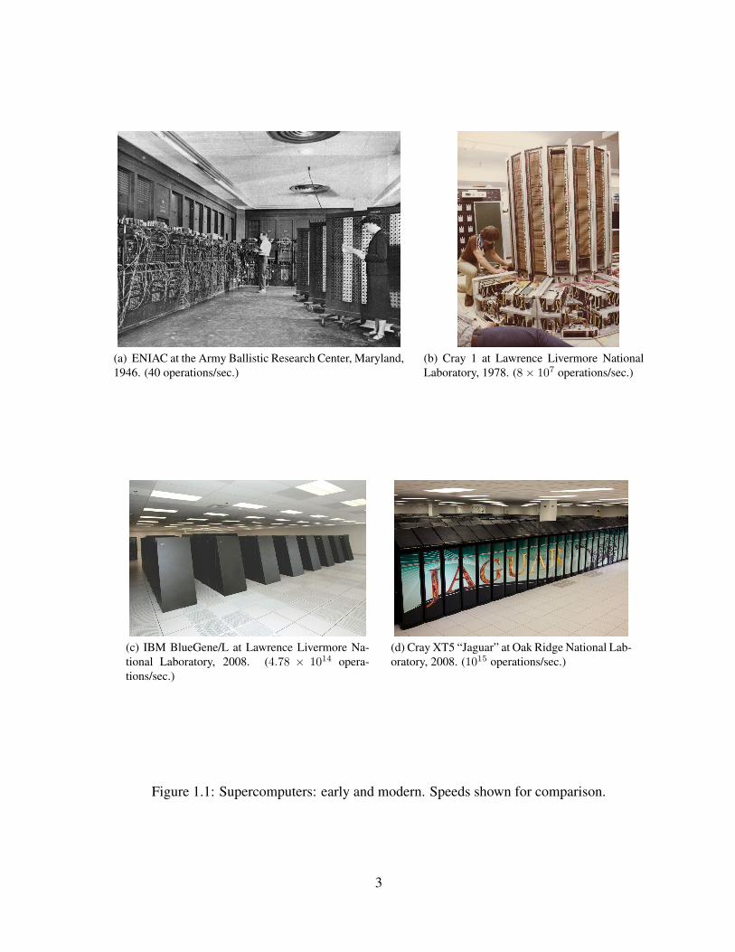
(a) ENIAC at the Army Ballistic Research Center, Maryland,1946. (40 operations/sec.)

(b) Cray 1 at Lawrence Livermore NationalLaboratory, 1978. (8× 107 operations/sec.)

(c) IBM BlueGene/L at Lawrence Livermore Na-tional Laboratory, 2008. (4.78 × 1014 opera-tions/sec.)

(d) Cray XT5 “Jaguar” at Oak Ridge National Lab-oratory, 2008. (1015 operations/sec.)

Figure 1.1: Supercomputers: early and modern. Speeds shown for comparison.

3

Supercomputers have evolved since the vector era. Modern machines exploit parallelism

at many levels. At a high level, they integrate large numbers of commodity processors so that

multiple instances of a single program may operate on different parts of a partitioned prob-

lem domain. This model of computation is called Single Program, Multiple Data (SPMD)

parallelism (Darema-Rodgers et al., 1984; Darema, 2001). Within each processor, super-

computers may also support vector instructions (Ramanathan, 2006). Alternately, they may

employ a co-processor, such as a Graphics Processing Unit (GPU) or a Field-Programmable

Gate Array (FPGA), that supports vector computation (Endo and Matsuoka, 2008). Today,

these instructions are implemented using multiple functional units, and the execution of sep-

arate operations within a vector instruction can proceed in parallel. This is called Single

Instruction, Multiple Data (SIMD) (Flynn, 1972) parallelism. Within each operation, func-

tional units themselves are pipelined. Finally, modern processors may support Instruction

Level Parallelism (ILP), where instructions from a sequential stream are processed out of

their original order, allowing more instructions to execute concurrently.

In this dissertation, we focus on performance measurement techniques for SPMD-parallel

machines. These machines have traditionally fallen into two categories: shared-memory

systems [or Symmetric Multiprocessing (SMP) systems] and distributed-memory systems.

Traditional SMP machines have a small number of processors with a shared address space.

Communication among processors happens through the memory system: either through main

memory or, more typically, through caches. As more processors are added to such a system,

the numbers of caches and memories grow, and coherence protocols must be used to maintain

consistency among them. Larger shared-memory machines typically employ a Non-Uniform

Memory Access (NUMA) architecture, where a shared address space is mapped in hardware

onto smaller, faster, physically distributed memories. In such a machine, each processor

has its own high-speed, local partition of memory, but accessing other processors’ partitions

is slower. NUMA machines have scaled to hundreds of processors, but fast memories of

4

1

10

100

1000

10000

100000

1e+06

1992 1994

1996 1998

2000 2002

2004 2006

2008 2010

Num

ber o

f Pro

cess

ors

MeanMaxMin

Figure 1.2: Concurrency levels of the top 100 supercomputers (Meuer et al., 2009).

sufficient size for larger systems cannot be built affordably.

Scaling problems with large shared memories led to distributed-memory parallel com-

puters. In distributed-memory systems, each processor has a local memory, but it is not

instruction-accessible from other processors. Processes running on distributed memory sys-

tems communicate by passing messages over a network. Systems built with this architecture

have come to be called clusters. They may be simple networks of commodity PCs connected

by commodity network links, or thousands of sophisticated, custom-built processors with

very fast, proprietary interconnects.

Clusters have been built with far more processors than can be attached to a single shared

memory, and it is this scalability that has led to their widespread adoption. In 1998, fewer

than 20 of the fastest 500 machines were clusters,1 and as of November, 2007, 410 of the 500

fastest machines (82%) employed this architecture.

Figure 1.2 shows concurrency levels over time for the top 100 supercomputers since 1993.

Cluster sizes have increased exponentially over the years, which has led to the creation of ex-

tremely large systems. The largest distributed-memory system in 2000 had slightly fewer

than 10,000 processors, but the largest in 2008, the International Business Machines Cor-

1According to performance on on the Linear Algebra Package (LINPACK) (Dongarra, 1987) benchmark, aslisted at Top500.org (Meuer et al., 2009).

5

poration (IBM) Blue Gene/L system at Lawrence Livermore National Laboratory (LLNL)

contains 212,992 processors, over twenty times as many. The current rate of growth is accel-

erating, and systems with millions of processors are expected to emerge within the next five

years.

1.2 Multicore Systems

The number of nodes in large clusters is not the only source of increased concurrency in mod-

ern systems. Recent trends in the microprocessor industry have led to concurrency increases

at the single-chip level, as well.

Gordon Moore first observed in 1965 that the transistors per unit area on processor dies

roughly doubled every year:

The complexity for minimum component costs has increased at a rate of roughly a factor

of two per year . . . Certainly over the short term this rate can be expected to continue,

if not to increase. Over the longer term, the rate of increase is a bit more uncertain,

although there is no reason to believe it will not remain nearly constant for at least

10 years. That means by 1975, the number of components per integrated circuit for

minimum cost will be 65,000. I believe that such a large circuit can be built on a single

wafer. (Moore, 1965)

Transistor counts have continued to increase at roughly the same rate since Moore’s observa-

tion, and the trend is now commonly called Moore’s Law.

Until recently, hardware designers used the extra transistors to improve sequential per-

formance by exploiting ILP. Clock speed has also increased, along with miniaturization of

chip components. However, chipmakers have reached physical limitations on pipeline depth

and power dissipation2, and the returns of sequential performance improvements have dimin-

2Technically, engineers have reached the limits of power dissipation acceptable for consumer parts. Com-modity processors are now used in supercomputers, so this is a concern at the high end, as well.

6

ished.

Additional transistors are now used to fit more independent processors, or cores on a sin-

gle chip, but this has several consequences for programmers. While Moore’s Law translated

to improved sequential performance, few changes were required for old code to take advan-

tage of new hardware, and application developers could expect the peak performance of their

programs to double in speed every 18 months as microprocessors became faster. Multicore

chips have the potential to provide similar speed improvements, but now programmers must

engineer their code explicitly to take advantage of task-level parallelism.

Multicore consumer chips have ramifications for scientific application developers at the

high end, as commodity technologies are typically used in the nodes of large clusters. Par-

allel application developers now face clusters of multicore nodes communicating via shared

memory among processors on the same node and through a fast interconnection network

among nodes.

1.3 Challenges for Performance Tuning

Extreme concurrency poses serious challenges for developers tuning large-scale applications.

The higher the number of concurrent tasks, the more difficult it is for programmers to exploit

available parallelism.

1.3.1 Amdahl’s Law

Amdahl’s law (Amdahl, 1967) tells us the maximum overall speed improvement we can

expect when part of an algorithm is improved. If we can speed up a percentage P of a system

by a factor of S, the expected speedup is:

1

(1− P ) + PS

(1.1)

7

The numerator here is the normalized running time of the original algorithm, and the denom-

inator is the normalized running time of the modified algorithm. (1−P ) gives us the running

time of the unmodified portion of the original algorithm, and P/S is the expected running

time of the improved fraction. For parallelization, we can rewrite this formula as follows:

1

(1− P ) + PN

(1.2)

P now represents the percentage of the original algorithm to be parallelized, and N is the

number of processors to be used, or the peak parallel speedup 3. Clearly, no matter how large

N becomes, speedup is limited by the sequential component of the algorithm, (1 − P ). For

example, if we can parallelize 96% of an algorithm, then we can expect it to speed up by no

more than a factor of 25.

1.3.2 Single-node Performance Problems

Performance tuning is the process of making an application perform well for specific hard-

ware. In large supercomputers, this can refer to problems either at the single node level, or it

may refer to problems arising from inefficient interactions between processes. The full range

of single-node performance problems is beyond the scope of this dissertation, but we give a

brief overview of the main concerns here.

On a single node, performance is dictated by several factors. First, problems may arise if

an application does not make efficient use of the local memory hierarchy. Modern machines

make extensive use of caches (Hennessy and Patterson, 2006a): small, fast memories with

faster instruction access time than main memory. If all of the data used by an algorithm does

not fit into cache at once, the processor must access main memory more frequently, which

can lead to significant slowdowns.

3For simplicity, we assume that these processors are homogenous.

8

Second, applications must take advantage of the specific instructions available on local

processors to achieve maximum performance. As mentioned, modern processors often sup-

port vector instructions, and if algorithms can be structured so as to perform several similar

operations at once, these may be fused into a smaller number of SIMD instructions. Alter-

nately, processors may be able to issue many different types of instructions at the same time

(ILP), and algorithms can be tailored to take advantage of this functionality (Hennessy and

Patterson, 2006b).

Finally, in the presence of shared memory and multithreading, node-local performance

may depend on the efficient synchronization of concurrent threads. This may depend strongly

on the speed of the memory hierarchy if threads use in-memory locking.

1.3.3 Inter-node Communication

Inter-node performance problems in large clusters arise from inefficiencies in communication

and synchronization among processes in parallel applications. Because modern clusters are

distributed-memory machines, they must employ interconnect fabrics to connect the mem-

ories of separate nodes. At the lowest level, communication performance depends on the

capacity of the physical network fabric. Immediately above the physical layer, latency and

bandwidth depend on the efficiency of the transfer and routing protocols used on the network.

Most supercomputers make use of some form of high-speed interconnect. Commodity

clusters typically use commercially available fabrics such as high-speed Ethernet (Metcalfe

et al., 1977; IEEE, 2005) or InfiniBand (Shanley, 2002) connected in a fat tree topology

with a hierarchy of switches (Leiserson, 1985). Other machines make use of one or more

custom interconnection networks. For example, the IBM Blue Gene systems use a tree-

structured network for collective communication and a three-dimensional torus for point-to-

point communication (Almasi et al., 2005). The Cray XT series machines make use of a

mesh network for collective and point-to-point communication (Vetter et al., 2006).

9

To develop distributed-memory parallel applications, application programmers do not

have to deal with high-speed networking protocols directly. Instead, they typically use a li-

brary to handle synchronization and message passing between processes. Currently, Message

Passing Interface (MPI) (MPI Forum, 1994) is the de-facto paradigm for large-scale parallel

computation, and it defines a set of operations for communication between two processes

(point-to-point communication) and among groups of processes (collective communication).

Programs written with MPI make wide use of synchronous constructs, per the Bulk Syn-

chronous Processing (BSP) model of parallel computation (Valiant, 1990). In the BSP model,

computation is organized into coarse-grained, alternating phases of computation and com-

munication. In computational phases, there is little or no inter-process communication, and

processes work on locally serial portions of a larger parallel problem. Once all processes

have completed a computation phase, state is exchanged in bulk during a communication

phase, and computation resumes.

The specifics of network operations are determined by the MPI implementor. Implemen-

tations can be designed to exploit the host machine’s native network architecture, but a poor

MPI implementation can be a source of serious performance problems in large-scale appli-

cations. For example, even on a high-bandwidth InfiniBand network, an implementation

of collective operations such as multicast must avoid congestion to achieve good perfor-

mance (Kumar and Kale, 2004).

Even with a well-tuned MPI implementation, the mapping of application processes to

nodes in a network topology may affect performance. In large-scale torus and mesh net-

works, the cost of communicating to distant nodes can be steep compared to the cost of

communicating with immediate neighbors. A good node mapping can decrease the average

number of hops required to send messages by placing frequently communicating application

processes close to each other on the network, thus improving performance

10

1.3.4 Load Imbalance

Harnessing the full power of a machine with millions of processors requires developers to

balance computational load by dividing the problem domain into units of equal (or approxi-

mately equal) amounts of work. Load balance is particularly important in synchronous sys-

tems because all members of a group of processes must complete a unit of work before any

process can continue. This implies that if one process takes more time to complete a particu-

lar task, all others must wait for it. In large systems, this may mean that a hundred thousand

tasks or more must idle.

Depending on the application, eliminating load imbalance may be trivial or it may prove

very difficult. Some problems are easily partitioned, and per-node behavior is static over the

course of a full run. However, the behavior of many modern applications can change over

time. For example, adaptive mesh refinement methods may increase the resolution of their

grids on some processes but not on others (Greenough et al., 2003; Colella et al., 2003b),

leading to more work for processes with refinement. Collisions between model elements and

other infrequent events in the simulation domain may give rise to transient computation.

Many applications employ dynamic load-balancing schemes to redistribute work among

processes at runtime, but these rely on precise data about the application’s work distribution.

As machines scale, this type of information becomes more difficult to collect, and load-

balance schemes may not scale efficiently.

1.3.5 Measurement

To evaluate the performance of applications running on large machines and to isolate per-

formance problems, engineers conduct detailed measurements of their applications. Perfor-

mance measurement is important because it enables programmers to decide which parts of

an application to optimize.

Measuring the performance of computer systems is difficult because it requires instru-

11

mentation, or modifications to source or binary code. By measuring, we modify the system

we observe. If we do not measure carefully, we may perturb the system’s behavior signifi-

cantly. Instrumentation code takes time to run and to record observations, and if it is executed

too frequently, the application may take much longer to run.

On large distributed-memory systems, measurement tools need a mechanism to store ob-

served performance data. The largest supercomputers increasingly use diskless nodes (Gara

et al., 2005; Vetter et al., 2006), so there may be no local storage on which to archive ob-

served data. Large machines typically are connected to a high-performance Input/Output

(I/O) system, but compute nodes typically communicate with the I/O system through the

same network used by applications. Perturbation becomes a problem when performance data

transport interferes with an application’s communication.

On large systems, this problem is magnified because every process may be monitored.

With each process monitored, the amount of performance data scales with the number of

processes in the system. Unfortunately, I/O bandwidth has not scaled as fast as core count,

and performance data from all processes could easily saturate an I/O system. If transport

routines within instrumentation must block on I/O, monitoring overhead can grow very large.

I/O overhead can be mitigated by reducing the volume of data exported from nodes to

disk, but there is a trade-off. With too little data, it may be difficult to ascertain at what

time or on which nodes a performance problem occurred. With too much data, issues of

practical storage and analysis remain. Per-process temporal data from systems with millions

of processors could be stored, but could consume petabytes of space. The data could be

mined for useful information in parallel, but the costs in disk storage and CPU time of such

approaches are prohibitive.

12

1.4 Summary of Contributions

To exploit the full computational power of future parallel machines, detailed measurements

are needed to guide design decisions around the obstacles outlined above. A system-wide

approach to measurement and optimization is needed; tools must collect enough data to cap-

ture the increasing complexities of on-node performance issues and to distribute work in a

large system effectively, but not so much data that I/O and networks are saturated or that

measurements are perturbed.

This dissertation details and evaluates novel techniques for measuring and analyzing per-

formance data on large-scale supercomputers. We apply these techniques to large-scale sci-

entific applications to illustrate their effectiveness, but the techniques themselves are more

generally useful. Parallel compiler developers, run-time authors, and application developers

alike may apply our monitoring techniques to understand and tune the performance of their

software on large machines.

The key contributions of this dissertation are as follows:

Scalable Load-balance Measurement. We present a novel technique for collecting two di-

mensional load-balance data in parallel applications across processes and over time.

This method draws on wavelet analysis from signal processing to compress system-

wide, time-varying load-balance data to manageable size. Results show that compres-

sion time is nearly invariant with system size on current I/O systems.

Sampled Trace Collection. We present a general technique using statistical sampling to

reduce the number of nodes that must be monitored in large systems, and we apply

this technique to parallel event tracing. Summary data from all processes is monitored

to estimate system-wide variance. The variance is then used to compute a minimum

number of sample nodes to enforce user-defined confidence and accuracy constraints.

Results show that the number of monitored nodes and the volume of traced data are re-

13

duced by one to two orders of magnitude for the system sizes tested. We also show that

clustering can stratify a heterogeneous set of nodes into homogenous groups, further

reducing trace overhead.

Combined Approach We combine the wavelet-compression and sampling approaches to

reduce load-balance monitoring overhead further. We use the data collected by our

scalable load-balance tool to guide on-line stratification of processes into performance

equivalence classes. We then use this information to reduce the sample size required

to monitor an entire system using our sampled tracing techniques.

Libra: An Integrated Analysis Tool. We have integrated our monitoring techniques into a

set of runtime tools and a GUI client for application developers. We show how the data

collected using our techniques can be used to diagnose a load-imbalance problem in a

large-scale combustion simulation. We further show that mining data collected using

Libra is feasible on a single-node system.

1.5 Organization of This Dissertation

The rest of this dissertation is organized as follows:

In Chapter 2, we give an overview of the fundamentals of performance measurement, and

we outline a framework for understanding different types of measurement and different types

of data. We then summarize previous work in performance measurement in the context of

this framework, and we summarize the limitations of existing tools and techniques.

Chapter 6 describes Libra, a scalable load-balance analysis tool. Libra makes use of the

Effort Model to represent load-balance data. We present the Effort Model and describe its

notions of absolute units of progress toward application goals and variable units of effort

expended to achieve those goals. We then describe how the model is applicable to a wide

range of scientific applications. Finally, we give a high-level overview of Libra’s software

14

architecture and its components.

In Chapter 3, we give a detailed description of Libra’s system-wide load-balance mea-

surement component. This component makes use of wavelet compression and is inspired by

techniques drawn from imaging and signal processing. To motivate the approach, we give an

introduction to wavelet analysis, and we show that the wavelet representation is particularly

effective for storing effort model data. Finally, we detail results of using this data collection

component to measure load-balance information for large-scale scientific applications. Re-

sults show that the method can achieve two to three orders of magnitude of compression with

modest error, and that the approach is scalable enough to measure very large systems.

In Chapter 4, we introduce techniques for sampled tracing, and we show how these can be

used for parallel performance analysis. To motivate this technique, we ground our approach

in statistical sampling theory, and we describe the scaling properties that uniquely suit it to

large systems. We then describe the architecture of Libra’s sampling component, and we

detail the results of using it with several large-scale applications. We also apply a technique

called stratified sampling, and we show that it can be used to further reduce trace overhead

in a sampled system.

Chapter 5 combines the ideas in Chapters 3 and 4 to adaptively stratify a running ap-

plication into performance equivalence classes. We use data from our wavelet compression

technique with scalable clustering algorithms to show that clusters produced can be used to

adaptively stratify traces on-line. We further show that dynamic stratification reduces the

sample size required to monitor a large system by up to 60% over a unified sampling ap-

proach.

Finally, in Chapter 7, we briefly summarize the work in this dissertation, and we state

conclusions that can be drawn from our results. We then briefly outline future research di-

rections that we plan to pursue based on this work.

15

Chapter 2

Background

2.1 Measurement and Optimization

Performance optimization is the process of making code run faster and more efficiently on

a specific system implementation. Modern systems can be tremendously complex, and op-

timization is difficult because it requires detailed knowledge of the components of these

systems and how they interact. It is not always apparent where in a system a performance

problem may lie, and detailed measurements are required to locate problems before optimiza-

tion is applied.

Choosing exactly what to measure requires that programmers understand the design of

computer systems. Modern systems are organized into vertical layers of abstraction. Each

layer hides implementation details of the layer below and provides a simplified interface to

the layer above. Programmers insert measurements at different levels in this hierarchy to

measure different aspects of a system’s functionality, and this process is called instrumenta-

tion.

Raw performance measurements can be copious, and to gain insight into application per-

formance, programmers must compile these measurements into more concise performance

characterizations. Creating a performance characterization usually involves a data reduction

step to focus on key observations in the set of measurements. Depending on the type of

characterization to be created, data reduction may involve discarding observations or it may

simply transform the observations into a representation more amenable to analysis.

In this chapter, we detail fundamental techniques for performance measurement and char-

acterization. To provide context, §2.2 describes the hierarchy of abstraction layers found in

modern computer systems and the interfaces used to connect them. §2.4 details fundamental

instrumentation techniques in the context of the abstraction hierarchy. We describe the types

of performance characterizations that may be produced from such measurements in §2.5, and

we detail generic techniques for data reduction in §2.6. Finally, §2.7 enumerates existing

performance tools and describes how they implement the techniques described here.

2.2 Abstraction

Modern computers are tremendously complex. The fastest microprocessors contain hundreds

of millions of individual transistors (Bright et al., 2005), and the operating systems that run

on them can contain millions of lines of code (Wheeler, 2002). Applications run on these

operating systems can contain further millions of lines of code and may make use of libraries

that contain millions more.

Integration at this scale is possible because software and hardware designers make exten-

sive use of abstraction: the process of factoring details from large problems and simplifying

them into general concepts. Each piece in a large system has a well defined interface for its

core behaviors, enabling other parts of the system to interact with it without concern for the

details of its design.

Figure 2.1 shows abstraction layers for a high-performance computing system. At the top

are application codes, which can access MPI and other libraries through publicly exported

Application Programming Interface (API) functions. API calls to libraries may be resolved

17

Application Codes

LibrariesLanguage Runtime

MPI

Hardware NetworkBlock StorageCPU Performance

CountersMemory

Operating SystemFilesystems

Device DriversInterrupt HandlersVirtual Memory

Figure 2.1: Computer system abstraction layers.

statically or dynamically, depending on the linkage mechanisms supported by the host Oper-

ating System (OS).

Libraries and applications can interact with the host OS through system calls. To the

user, system calls appear as ordinary functions, but beneath this abstraction they implement

a control transfer from user code to the underlying OS kernel. The control transfer allows

potentially unsafe operations to be encapsulated within the operating system, and prevents

applications from interfering with each other. Operating systems usually provide an inter-

mediary library to handle details of system call implementation; on UNIX-like operating

systems, the C language runtime library handles this task.

System calls can incur more overhead than other library function calls, as the control

transfer may require hardware interrupts and parameter data may need to be copied from

user space to kernel space. This is not true of all machines. Some high-performance ma-

chines (Gara et al., 2005) trade strict separation of memory between the OS and applications

for performance.

The operating system mediates interactions between software and hardware. This in-

18

cludes process control and managing access to shared hardware resources. Such resources

are exposed to the user through abstractions. For example, when users make system calls to

manipulate a local filesystem, the OS translates these calls to block storage commands and

communicates with a disk drive on the caller’s behalf. Alternately, filesystem calls may be

translated to network requests to access storage on a remote machine.

The operating system may allow users to register interrupt handlers to respond to asyn-

chronous events. This enables applications to execute user code at a predetermined interval

using a timer interrupt. On systems with more extensive hardware support, interrupt handlers

may also be registered for performance-counter-related events.

2.3 Scalability

For large parallel scientific codes, the ability of an application to make efficient use of its

interconnection network plays a large role in performance. Running a code on increasingly

larger systems is called scaling, and a code’s ability to communicate efficiently as the number

of nodes in a system increases is referred to as scalability.

The scaling behavior of scientific applications is typically defined in terms of the relation-

ship between the size of a computing system and the size of the problem on which it operates.

In scientific simulations, the problem size is generally given as the number of model elements

being simulated. For example, in a molecular dynamics simulation, the amount of compu-

tation necessary to simulate a fixed amount of time depends on the number of molecules

simulated. Alternately, a gas dynamics simulation might model a volume of gas as a dis-

cretized mesh, in which case problem size is defined by the number of mesh elements in the

simulation.

There are two primary scaling behaviors for parallel applications:

Strong Scaling refers to increasing the system size (number of processors) while holding

19

the problem size fixed. With ideal strong scaling, execution time will decrease propor-

tionally to processor count as more processors are added to a system. Strong scaling

inefficiencies arise when communication costs increase as more processors are added,

or when model granularity is too small to allow even partitioning across all processes in

the system. Amdahl’s law dictates that, in the limit, execution time will be dominated

by the sequential components of computation in such systems.

Weak Scaling refers to increasing problem size proportionally with system size as more

processors are added to a system. With perfect weak scaling, execution time remains

constant as system size is increased. Adding more processors to a weak scaling system

increases the problem size that can be calculated in the same amount of time. This is

useful when more detail or more elements are needed to simulate large physical sys-

tems accurately, as opposed to allowing fixed-size problems to be solved more quickly,

as in strong scaling.

2.4 Instrumentation

Code or hardware added to a system to record measurements is called instrumentation. In-

strumentation can be applied at any level of the abstraction hierarchy, depending on what is

to be measured. This section discusses fundamental techniques for instrumentation and the

trade-offs associated with each of them.

2.4.1 Hardware Instrumentation

At the lowest level, measuring the running time of an application requires some hardware

support. Nearly all computers produced today have on-board clocks that can be used to

measure time intervals at millisecond resolution. However, since most processors today run

at hundreds of megahertz or multiple gigahertz, this is not sufficient to measure many low-

20

level hardware events accurately. Most systems therefore include higher-resolution timing

registers to measure tighter intervals in terms of elapsed CPU cycles. Depending on the

access method, such interval timers can offer precision in the microsecond or nanosecond

regime.

Depending on the system, more extensive hardware counters may be available. Many

modern processors provide a configurable set of registers called Hardware Performance Mon-

itors (HPM) that can record counts of hardware events. Events themselves are monitored

through special detectors integrated into the processor itself. Inputs from detectors are multi-

plexed and connected to registers, and users can configure the registers to count events such

as memory references, cache misses, Translation Lookaside Buffer (TLB) misses, branch

mispredictions, instructions and network operations.

2.4.2 Trace Instrumentation

To use hardware instrumentation, and to take measurements while a program is running,

instructions for measurement must somehow be inserted into the control flow of a running

system. One method of doing this is to insert instructions in the control flow of an application

or library itself, so that those instructions will be performed in the course of the application’s

normal execution. Instrumentation routines inserted this way may measure intervals with the

timers described above, or they may simply record the occurrence of some software event.

Such techniques are called tracing.

Source Code Instrumentation

A straightforward way to make sure that instructions are executed at certain points in a pro-

gram’s control flow is to insert calls to instrumentation routines directly into the source code

and compile them along with the program itself. This is called source code implementation.

Programmers often use this sort of instrumentation in the course of debugging application

21

code when they add statements to output data to the screen or to a file. This allows program-

mers to observe the order of events at runtime as they occur. However, inserting source code

instrumentation by hand may be tedious if a large number of routines in a program are to be

measured. In such cases, a parser may be used to insert calls to measurement routines into

source code automatically. The modified source code then can be compiled and run to take

measurements and to record events.

Source code instrumentation can be applied to any software, including applications, li-

braries, and operating systems, provided that the source code is available. On some systems,

instrumenting at lower levels of abstraction may be difficult, depending on what rights the

user has on a system. For example, it may be difficult and time-consuming to instrument, re-

compile, and install a new operating system on a production machine. Likewise, proprietary

library source code may be unavailable to the end user.

Source code instrumentation is a static technique. When measurement code is compiled

with an application, the application is perturbed slightly when the instrumentation is exe-

cuted. The amount of perturbation depends on what specific actions the instrumentation

performs and how frequently it is executed in the course of a run. Guard statements can be

placed around instrumentation code to effect dynamic enablement and disablement of the ac-

tual measurements. Even if instrumentation is disabled, guard statements still require a small

amount of time to execute, so there is no way to avoid this probe effect completely.

Binary Instrumentation

Another technique for inserting instrumentation into a system’s control flow is to modify its

object code. This is called binary instrumentation. Like source code instrumentation, binary

instrumentation adds instructions that are executed along with those of the program.

Source-level instrumentation lets the compiler generate new object code from instru-

mented source files, but binary instrumentation modifies instructions in object code directly.

22

Typically, an instruction at the beginning of an instrumentation point is replaced with an

unconditional jump, which transfers control to special instrumentation code called a trampo-

line function. The trampoline then runs to completion and jumps back to just after the point

where control was diverted. Binary instrumentation may be performed statically before an

executable runs, or it may be performed by modifying a running process’s memory through

a debugger interface.

One advantage of binary instrumentation is that there is no probe effect when it is not

enabled because the instrumentation is never executed. In addition, it can be applied to

unmodified object code without recompiling, but the object code must be modifiable by the

instrumentor. Thus, it may be impractical in production systems to instrument system code

or kernel routines using this technique, but some operating systems support adding limited

dynamic instrumentation to kernel routines.

Link-level Instrumentation

We have discussed techniques for inserting trace instrumentation by modifying source code,

binaries, and running processes. A final mechanism for injecting instrumentation in an ap-

plication’s control flow is to use the linker.

If an application makes use of a particular library, its calls to those libraries must be

resolved by either a static linker or a dynamic loader. Programmers can make a custom

library that implements wrappers for function calls of the measured library. If the application

is linked with the modified library, its library calls will resolve to instrumentation routines,

and the unmodified application code can run with an instrumented version of the library.

Link-level instrumentation is useful for measuring the interactions of an application with

particular libraries. It is used frequently to measure codes that make use of MPI. The MPI

specification itself includes a name-shifted “PMPI” interface to all calls, so that wrapper

libraries can easily intercept MPI function calls and delegate to their “PMPI” equivalents

23

after executing instrumentation.

Link-level instrumentation is convenient for the programmer in that it does not require

that the measured application be recompiled. If only static linking is available, it is necessary

to re-link an application. With dynamically linked libraries, this may not be necessary. Many

operating systems support for forcing an instrumentation library to be loaded at the start of

runtime (e.g. via the LD PRELOAD environment variable in Linux). Loading a library at

this point forces library calls to resolve to routines in the instrumentation library, even if the

original library is also loaded.

2.4.3 Sampling

We have discussed several techniques for trace instrumentation. In addition to tracing, we

may also elect to use sampling to measure computer systems and applications.

Sampling is a form of asynchronous instrumentation. Instead of embedding instructions

directly into an application’s control flow, as in tracing, we take periodic measurements, or

samples, asynchronously. Depending on how samples are taken, they can be used determine

where an application is spending its time or where it consumes a particular resource.

Typically, sampling is implemented by registering interrupt handlers with the operating

system. Most systems support periodic timer interrupts, where execution is interrupted at

a regular interval over time. Depending on hardware support, there may be other, finer-

grained interrupt mechanisms for tools to use. For example, many systems allow users to

register interrupt handlers to be called after a certain number of CPU cycles. For systems

with HPM counters, many systems also allow hardware counter interrupts, such that code

can be sampled periodically according to instances of particular hardware events.

Sampling may be used throughout a system, although, as with other techniques, there are

privilege-level issues associated with sampling the operating system. Kernel-level interrupt

handlers need to be compiled into the OS or loaded as a module, which may not be possible,

24

depending on the particular installation. For application and library code, however, at least

timer interrupts are supported on most current platforms.

2.4.4 Trade-offs

Sampling and tracing are complementary techniques. Tracing allows the programmer to

observe events as they happen at runtime, since instrumentation is embedded directly into a

system’s control flow. This allows for more complete coverage. With trace instrumentation,

an instrumented function is guaranteed to be observed each time control passes to it, and we

know that the events recorded are exactly those that occurred at runtime. With sampling,

there is no such guarantee.

Trace instrumentation can incur significant probe effects if the routines instrumented are

executed frequently, which may make very fine-grained traces of applications cumbersome

or infeasible. If a tight loop is instrumented with costly trace instrumentation, an application

can take many times its original running time to finish, which may distort performance mea-

surements. Some tools take a complementary approach and measure only particular routines

so that trace instrumentation is sparse and the application is unperturbed.

The cost of sampling is a trade-off between overhead and sampling error. If the sampling

rate is too low, infrequent events can escape observation. If the sampling rate is too high, an

application can be perturbed severely. Typically, sampling tools take the middle ground here,

using a sampling rate that incurs little overhead but still achieves reasonable code coverage.

2.5 Performance Characterization

Before measurements can be of use in guiding optimization, they must be compiled and

aggregated into concise descriptions called performance characterizations. Like instrumen-

tation, there are many different techniques for characterizing performance, and the technique

25

selected guides the type of instrumentation used for measurement.

2.5.1 Profiling

Profiling is a technique used to map regions of source or object code to the amount of a partic-

ular resource they consume. In the most common case, the resource measured is cumulative

time, but profiles may also be generated from HPM measurements.

There are two general types of profiles. Flat profiles are direct mappings from static

code regions to the time they consume. This type of mapping does not take dynamic calling

context into account, so the time attributed to a particular region in a flat profile is the time

spent in that region regardless of where it was called. Call-path profiles attribute time to

particular calling contexts. This can be useful if selected functions are called from multiple

places within an application. For example, if a given solver is used for two phases of a

complex physics code, a call-path profile can provide insight into which context takes the

most time to solve.

Both types of profiles may be generated either from trace measurements or from sam-

pling. For a full call-path profile to be generated with trace instrumentation, all function

entry and exit points must be instrumented. Excessive perturbation can result if some func-

tions are called too frequently.

Sampling can be used to generate statistical call-path profiles if facilities are available

to unwind a program’s call stack. This can be a costly operation, and in the presence of

optimization (e.g., from compilers), it may be difficult or impossible to unwind the stack

completely. Sampled flat profiles are simpler to generate in that they require only that the

Program Counter (PC) be recorded.

Profiles may be generated at various levels of granularity, depending on the precision

desired by the implementor. As mentioned, sampled profiles record the PC that was sampled,

which may be mapped to a particular instruction in the source code. More frequently, though,

26

PCs are mapped to statements in source code or to particular functions, giving a higher-level

view of where a program spends its time. The granularity of profiles generated from trace

data depends on the granularity of the trace instrumentation itself.

2.5.2 Tracing

A trace is a performance characterization generated from observations of performance events

(e.g., those recorded by trace instrumentation) over time. Unlike profiles, which discard time

information, a trace can capture the full sequence of events in a program’s execution.

Traces can be useful in determining evolutionary behavior in simulations. For example,

model data in a parallel simulation may change significantly as the simulation progresses.

After some time, more work may be required on some processes than others, and aggregating

results over time may discard such potentially useful information. Likewise, traces can be

useful for analyzing the correctness of a program’s execution, because they give a precise

ordering of events. This is difficult with profiles, because timing information, and thus insight

into causality, is discarded.

The added information present in traces comes at a price in terms of space. Whereas

single-process profiles are relatively compact (their size is a function of static code size),

traces grow with the length of a run. This can consume very large amounts of disk space.

2.5.3 Phased Profiling

Profiling and tracing are complementary techniques, and attempts have been made to com-

bine them in phased profiling. Phased profiling records profiles for predefined time windows

over the course of an application’s execution. This allows application developers to see the

behavior of their applications evolve over time, yet it can consume considerably less space

than a full trace, depending on the window size used.

Some phased profilers require manual instrumentation to signal to the tool that one phase

27

has ended and that another has begun. Techniques have also been developed to detect phases

in code automatically. These techniques use statistical analyses on performance metrics to

differentiate the behavior of the code at different times during execution. Such tools have

applications to performance monitoring for phased profile analysis. They also have been

applied to the computer-architecture design process in the SimPoint (Perelman et al., 2006)

tool. This tool is described in more detail in §2.7.7.

2.5.4 Performance Modeling

Profiles and traces are not the only forms of performance characterization, but they are two

of the most widely used in the field of performance analysis. Other techniques have been

developed to predict the performance of future runs of applications based on historical data.

This section describes some of these techniques.

Compile-time Scalability Analysis

Mendes and Reed (Mendes and Reed, 1998) present a methodology for assessing the scal-

ability of applications based on information gathered at compile time. Specifically, they

modified a Fortran D95 compiler (Adve et al., 1994; Wang et al., 1995) to convert all loops

in a program to symbolic expressions in terms of problem size and number of processors. The

compiler also gathers information on the instruction distribution within loops. Costs of in-

structions as well as of send and receive operations are evaluated offline by machine-specific

meta-benchmarks. A sum of loop send, receive, and instruction breakdowns weighted by

these costs is used to predict upper and lower bounds for total program execution time.

Mendes and Reed show that by computing costs for different machines, their model can

be used as a reliable estimate for execution time across architectures. Moreover, they show

that their approach can be used to locate bottlenecks in code. By comparing estimated ex-

ecution times for individual loops in the same program, they are able to detect loops that

28

dominate execution time. This information can guide performance engineers to places in the

code that need optimization.

Convolution-based Performance Prediction

Snavely et al. demonstrate that application performance can be modeled locally by exam-

ining memory hierarchy behavior, since the ability of a code to manage memory effectively

dominates local performance (Snavely et al., 2001). However, modern architectures use in-

creasingly complex hierarchies of caches, and it is unlikely that an application that has a

certain memory performance on one architecture will have similar performance on another.

Snavely et al. use a benchmark to evaluate sustained load and store performance for a sin-

gle processor with various memory access patterns. Based on the results of this benchmark,

they create a mapping from access parameters to benchmark performance.

The authors then use a simulator to generate basic block profiles of scientific codes. The

simulator can be configured to reflect the memory hierarchy of arbitrary architectures, and it

gives cache-miss rates for each basic block in the simulated code.

Convolution is applied to combine the miss rate profile for basic blocks with the memory

profile, and the result can be used to predict the execution time of applications. The authors

profile sequential kernels from the NAS Parallel Benchmarks (NPB) (Bailey et al., 1991),

and their method predicts execution times within 4% error. When extended to predict the

time of parallel codes, it is accurate to within 20%.

Though this is a profile-based approach, the overhead of the method is considerably

greater than that of a typical profile approach because it records memory references. Pro-

filing memory references is impractical for monitoring large production systems, since it can

increase execution time by orders of magnitude.

29

2.6 Data Reduction

Because computer systems are complex, the space of potential performance measurements is

large and many-dimensional. A single process can generate more data than is convenient for

humans to digest, and a large parallel machine can produce far more than this.

Because of this complexity, we must be judicious in choosing the measurements that we

take and in deciding how much data to record. Ideally, we would record just enough perfor-

mance data to diagnose a problem, but we may not know on which processes or in which

parts of a run a performance problem may arise. Recording all available performance data

can be impossible, as in the case of HPM counters, where not all values may be monitored at

once; or impractical, as in the case of large traces, where disk space and data-mining capacity

comes at a steep cost.

Performance tools make use of a variety of techniques for data reduction. In this section,

we describe these techniques and the trade-offs involved in each.

2.6.1 Data Compression

Data compression is any technique that reduces the number of bits needed to store informa-

tion. Data converted to such a representation is encoded, and when it has been returned to its

original representation, it is decoded.

Lossless Compression

Lossless compression refers to compression after which the original representation can be

reconstructed exactly from the encoded representation. Lossless compression relies on the

fact that most real-world data has at least some statistical redundancy.

Lossless compression is rooted in information theory. The Shannon entropy (Shannon,

1948), a measure of the average information content in a message, represents the upper bound

30

on how compactly data can be represented using such techniques.

Entropy encoding is one of the most common forms of lossless compression. Two exam-

ples of entropy coding are Huffman coding (Huffman, 1952) and arithmetic coding (Rissanen

and G. G. Langdon, 1979). These techniques both rely on the higher probability of encoun-

tering some symbols than others in the input data. More frequently occurring input symbols

are are represented with smaller output symbols and less frequently occurring symbols with

larger output symbols, thus reducing the size of the representation.

Other lossless compression algorithms may use statistical models or dictionaries to record

frequently occurring patterns in the input data. The simplest example of such an encoding is

Run-Length Encoding (RLE), which stores contiguous runs of a symbol in the input data as

the symbol and an associated number of repetitions. Other encoding schemes use more so-

phisticated dictionary lookup schemes, as in Lempel-Ziv-Welch (LZW) (Welch, 1984) cod-

ing.

Lossy Compression

As mentioned, Shannon entropy bounds the compression that can be achieved if an input

representation is to be compressed and then reconstructed exactly. However, lossy compres-

sion can allow for much greater reductions in data volume, if the user is willing to accept an

approximate reconstruction of the original data.

At a high level, lossy compression is similar lossless compression, in that the goal of the

compression is to reduce redundancies in the input data. Instead of considering the input as

a stream of symbols, as with lossless techniques, lossy compression techniques treat their

inputs as raw numerical data and use basis transforms to project inputs inputs into domains

where they can be represented more sparsely. Transformed data is then encoded in such

a way as to prioritize the most significant coefficients in the transformed output, possibly

discarding less significant values.

31

Lossy compression techniques offer a trade-off between data volume and accuracy. The

more data that an encoder writes to disk, the more closely the output representation can

be reconstructed to mirror the original inputs, and vice versa. Users of lossy compression

schemes can typically set a compression level to control the trade-off.

Lossy techniques have been applied widely to process image, video, and audio signal

data. The popular JPEG image compression format, the MPEG video compression format,

and the MP3 audio compression format all use a Discrete Cosine Transform (DCT) coupled

with lossy encoding to reduce the size of media files significantly. Similarly, the JPEG-

2000 (Adams, 2002) image format uses a discrete wavelet transform coupled with lossy

coding techniques.

Lossy compression also may be employed for performance tracing. Lu and Reed present

the application signature (Lu and Reed, 2002), a technique that represents numerical trace

data concisely. Given a time-ordered sequence of metric values gathered at runtime, its

signature is a piecewise-polynomial approximation of this sequence.

Signatures are constructed dynamically, and programmers can adjust an error threshold

to modulate recorded trace size. Larger error thresholds will cause the fitting algorithm

to generate a more compact signature at the expense of accuracy. Likewise, smaller error

thresholds lead to larger, more accurate signatures. An exhaustive trace is a signature with

error threshold of zero.

Lu and Reed show that performance of parallel applications can be validated using ap-

plication signatures. An application is run once under ideal conditions and a signature is

recorded. When the application is run again, another signature can be recorded, and pro-

grammers can compare the two to determine whether performance of the new run meets or

exceeds the original. Lu and Reed describe a time-normalized function for assessing sig-

natures’ behavioral similarity, which they use to determine whether applications have per-

formed similarly on different hardware architectures.

32

2.6.2 Population Sampling

Population sampling is a technique for estimating the behavior of a set by observing only

a fraction, or sample, of its elements. Traditionally used in polling and survey research,

sampling is useful because it can reduce the cost of data collection significantly if collecting

observations is expensive. Because it reduces the number of observations that need to be

made, sampling is also useful for reducing data volume.

The minimum sample size for a population with constant variance scales more slowly

than the population itself, allowing one to sample comparatively small numbers of nodes for

accurate estimates of very large populations. Notably, for N monitored processes, fixed error

bound d, and desired deviations from the estimator mean zα, a sample size of n is required,

where n satisfies:

n ≥ N

[1 +N

(d

zαS

)2]−1

(2.1)

Typically, confidence and accuracy of sample surveys are computed after the survey is

complete, from the size of the sample taken. Equation 2.1 can be applied to reverse this

process. The user specifies desired confidence and error bounds, and the required minimum

sample size for meeting these bounds is computed. The user then has a probabilistic guar-

antee that his estimation will be accurate. Furthermore, sampling scales very well to large

quantities of nodes. Note that as N increases, n approaches (zαS/d)2. This implies that

sample size is proportionally smaller for very large numbers of processes.

Mendes and Reed (Mendes and Reed, 2004) have shown that sampling-based monitoring

techniques are useful for monitoring large sets of distributed machines. They monitored the

availability of a cluster of 1464 processors and showed that at normal load levels this can be

measured with 90% confidence and 5% error by considering the machine as a population of

processors and sampling only 16% of the processors. Similarly, they showed that the free

node percentage for a cluster of 3008 processors can be measured with 90% confidence and

33

8% error while only sampling 1.5% of the total number of machines.

Since collected data volume is proportional to the number of processes, this technique

can reduce monitoring overhead in large clusters substantially.

2.6.3 Cluster Analysis

Cluster analysis refers to a number of statistical algorithms for finding homogeneous groups,

or clusters, within data. Like other techniques described here, clustering relies heavily on

statistical redundancy in input data. While typically not described as a data reduction tech-

nique per se, clustering can be useful for data reduction because it allows large data sets to

be described in terms of a smaller number of clusters.

Two widely used techniques for clustering are hierarchical, or agglomerative, clustering

algorithms (Kaufman and Rousseeuw, 2005a), and partitional clustering algorithms (Kauf-

man and Rousseeuw, 2005b; Kaufman and Rousseeuw, 2005c; Forgy, 1965; Hartigan and

Wong, 1979; Lloyd, 1982). Users of both of these algorithms define a distance measure on

the input data, which is used by the algorithms to determine the similarity of pairs of objects

in the input data. In hierarchical clustering algorithms, groups of objects are merged recur-

sively, producing a hierarchical tree of clusters with increasing granularity. In partitioning

algorithms, the number of clusters, k, is specified in advance, and the algorithm attempts to

find a group that fully or nearly minimizes the distance between objects in k clusters. We

describe techniques for cluster analysis in more detail in §5.2.2.

Ahn and Vetter (Ahn and Vetter, 2002) show that cluster analysis is useful for detect-

ing load imbalance when applied to HPM data. Specifically, they are able to detect small

communication-related load imbalances between edge, corner, and other processes in a two-

dimensional physics simulation. Cluster analysis thus enables a 256-process system to be

described in terms of these three homogeneous groups.

34

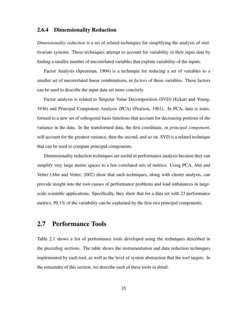
2.6.4 Dimensionality Reduction

Dimensionality reduction is a set of related techniques for simplifying the analysis of mul-

tivariate systems. These techniques attempt to account for variability in their input data by

finding a smaller number of uncorrelated variables that explain variability of the inputs.

Factor Analysis (Spearman, 1904) is a technique for reducing a set of variables to a

smaller set of uncorrelated linear combinations, or factors of those variables. These factors

can be used to describe the input data set more concisely.

Factor analysis is related to Singular Value Decomposition (SVD) (Eckart and Young,

1936) and Principal Component Analysis (PCA) (Pearson, 1901). In PCA, data is trans-

formed to a new set of orthogonal basis functions that account for decreasing portions of the

variance in the data. In the transformed data, the first coordinate, or principal component,

will account for the greatest variance, then the second, and so on. SVD is a related technique

that can be used to compute principal components.

Dimensionality reduction techniques are useful in performance analysis because they can

simplify very large metric spaces to a few correlated sets of metrics. Using PCA, Ahn and

Vetter (Ahn and Vetter, 2002) show that such techniques, along with cluster analysis, can

provide insight into the root causes of performance problems and load imbalances in large-

scale scientific applications. Specifically, they show that for a data set with 23 performance

metrics, 99.1% of the variability can be explained by the first two principal components.

2.7 Performance Tools

Table 2.1 shows a list of performance tools developed using the techniques described in

the preceding sections. The table shows the instrumentation and data reduction techniques

implemented by each tool, as well as the level of system abstraction that the tool targets. In

the remainder of this section, we describe each of these tools in detail.

35

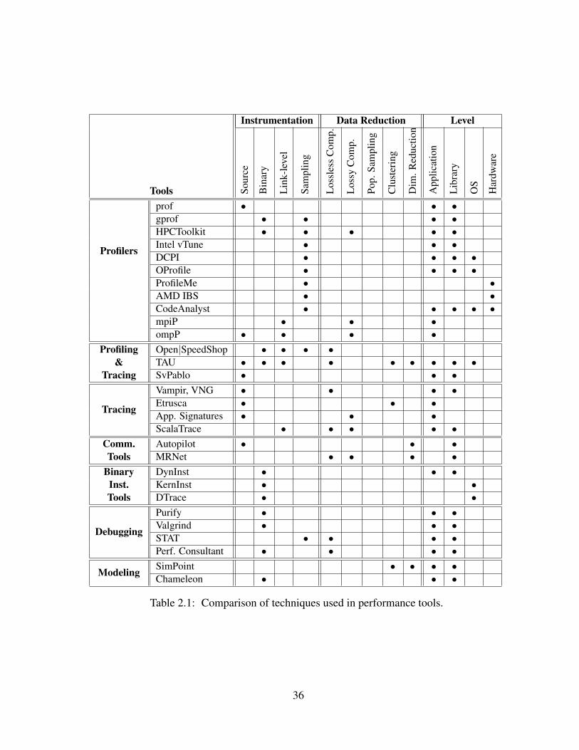
Instrumentation Data Reduction Level

Tools Sour

ce

Bin

ary

Lin

k-le

vel

Sam

plin

g

Los

sles

sC

omp.

Los

syC

omp.

Pop.

Sam

plin

g

Clu

ster

ing

Dim

.Red

uctio

n

App

licat

ion

Lib

rary

OS

Har

dwar

e

Profilers

prof • • •gprof • • • •HPCToolkit • • • • •Intel vTune • • •DCPI • • • •OProfile • • • •ProfileMe • •AMD IBS • •CodeAnalyst • • • • •mpiP • • •ompP • • • •

Profiling Open|SpeedShop • • • •& TAU • • • • • • • • •

Tracing SvPablo • • •

Tracing

Vampir, VNG • • • •Etrusca • • •App. Signatures • • •ScalaTrace • • • • •

Comm. Autopilot • • •Tools MRNet • • • •

Binary DynInst • • •Inst. KernInst • •Tools DTrace • •

Debugging

Purify • • •Valgrind • • •STAT • • • •Perf. Consultant • • • •

Modeling SimPoint • • • •Chameleon • • •

Table 2.1: Comparison of techniques used in performance tools.

36

2.7.1 Profiling Tools

prof

prof is a flat profiler traditionally implemented as part of the compiler in UNIX operating

systems. Programmers supply an extra flag (+prof), and the compiler emits object code

containing wrapper functions that output profile files when the program is run.

gprof (Graham et al., 1982) and GNU gprof (Fenlason and Stallman, 1988) are de-

scendants of prof included in most UNIX-like operating systems and supported by most

compilers today. As with prof, programmers supply an additional flag and the compiler

emits a special profiling version of the executable. gprof supports a limited form of call-

path profiling in which only the first ancestor is recorded.

At runtime, gprof sets a timer interrupt handler to execute roughly 100 times per second.

It also inserts binary instrumentation around procedures in the object code. The handler

samples the PC and records its value in a histogram. When execution is complete, gprof

has sample counts for each PC in the program, which are used to estimate what percentage of

runtime was spent in each part of the code. gprof and GNU gprof build on this function

by also recording call-path information.

HPCToolkit

HPCToolkit (Mellor-Crummey, 2003) is a suite of tools for sampled, profile-based perfor-

mance analysis. It includes tools for gathering profile data and for correlating program struc-

ture (e.g., loops, procedures, and statements) with profiles. HPCToolkit minimizes overhead

in two ways. First, instead of using a timer interrupt, it uses counter interrupts to guide in-

strumentation. Counters are set to overflow mode so that they generate an interrupt when

their register value overflows. The register’s value is then set to the maximum value minus

some frequency, so that the counter will overflow only after a chosen number of observed

37

events. The user can control overhead by adjusting this frequency.

By using counter interrupts instead of timer interrupts, HPCToolkit allows a wider range

of profiles to be taken. For example, one could generate a time-based profile by using the

cycle counter’s overflow to trigger sampling, or one could generate a profile locating the

highest rate of execution of floating point instructions by setting the floating point event

counter as the trigger. Counter interrupts require hardware support, so this functionality may

not be available on all platforms.

In addition to flat profiles, HPCToolkit contains optimizations for efficient call-path pro-

filing (Froyd et al., 2005; Froyd et al., 2006). Typically, recording a call path requires that the

tool examine the stack to determine which call frames are present. Naıve implementations

walk the full stack on every interrupt, which can incur unnecessary overhead in programs

with deeply nested calls.

HPCToolkit uses a simple form of binary instrumentation to assist in the stack-walking

process. When the first interrupt occurs, the stack is examined and its frames are recorded.

Then, the return address of the top function on the stack is replaced with a pointer to a tram-

poline function. When the top function returns, control is transferred to the trampoline, which

replaces the return address of the next function in the stack with a pointer to the trampoline

and adjusts the recorded list of stack frames.

The trampoline pointer in HPCToolkit acts as a high-water mark by indicating to the stack

unwinder that all frames below it in the stack are already known. Thus, when subsequent

interrupts occur, the unwinder only needs to conduct a detailed examination of frames above

the trampoline pointer. It can then concatenate these frames with the prefix recorded by the

trampoline function to get a full stack trace.

HPCToolkit currently outputs one profile per instrumented process, but lossy compres-

sion may be applied to these profiles post-mortem to generate a single, global profile (Bor-

delon, 2007). Merging provides the user with concise summary information for an entire

38

parallel run, but the profiling process discards temporal data, and records of inter-process

variation are discarded. Alternately, the user may apply cluster analysis to stored per-process

profiles (Bordelon, 2007), which can reveal behavioral equivalence classes among processes.

Intel VTune

VTune is a commercial set of tools developed by Intel for profile-based performance analy-

sis. It includes tools for both flat and call-path profiling using sampled instrumentation.

OProfile

The profilers mentioned so far operate on a single process or on a set of parallel processes

in user space. OProfile (Levon and Elie, 2008) is a system-wide sampled profiler designed

to measure user-space processes, kernel activity, and libraries. Like HPCToolkit, it does

not require modification of application binaries. It differs from HPCToolkit and the prof

family of tools in that it is capable of sampling an entire running operating system and all

of its processes. Output from OProfile includes histograms from shared libraries and can

reflect how they are used by different applications. It can also provide greater insight into

contention for system resources. It can provide both flat profiles and callgraph output. At the

time of this writing, however, OProfile required root access to a system, making it difficult to

use with institutionally managed high-performance machines.

OProfile is a descendant of the Digital Continuous Profiling Infrastructure (DCPI) (An-

derson et al., 1997) and SpeedShop (SGI, 2003), two earlier full-system profilers.

ProfileMe. ProfileMe (Dean et al., 1997) is a hardware-supported profiling technique im-

plemented on the Alpha 21264 microprocessors (Dean et al., 1997) that allows individual

instructions to be sampled through their entire execution rather than simply sampling the PC

register.

39

This type of sampling allows more detailed analysis of the behavior of out-of-order pro-

cessors because it exposes details that must be inferred from a combination of counters with

other profiling tools. For example, with ProfileMe, pipeline stalls can be attributed to specific

instructions, which is difficult with standard hardware performance counters because instruc-

tions are not directly tied to performance events. In most processors, event counters are not

guaranteed to be incremented until sometime after the instruction that generated an event has

completed.

AMD CodeAnalyst Tools

While sophisticated, ProfileMe requires very specialized hardware support. Until recently,

no chip since the Alpha had attempted to implement such a sophisticated scheme.

AMD Instruction-Based Sampling (AMD-IBS) (Drongowski, 2007) is a new implemen-

tation of instruction-based sampling used in newer AMD microprocessors. It is used in con-

junction with OProfile to implement the profiling component of AMD’s CodeAnalyst suite

of performance tools (Advanced Micro Devices, 2009). Like ProfileMe, AMD IBS enables

attribution of performance problems to specific pipeline stalls and other events with sub-

instruction granularity.

mpiP

mpiP is a tool for profiling communication calls in MPI applications. mpiP is implemented

as a library containing profiling wrappers for MPI communication calls. The user links

against this library, and the wrapper functions record statistical information about all MPI

calls in the program. mpiP records calling context information for each monitored MPI call.

At the end of a run, per-process profiles are merged into a single output file.

Vetter et al. present a statistical technique for finding scalability problems in scientific

codes using mpiP (Vetter and Chambreau, 2005). They use the tool to profile communication

40

events; then, they compute the correlation between percentage of total time taken by each

call and the number of processes in each run. To compensate for outliers and non-normal

distributions of event durations, they do not compute this correlation directly. Rather, they

find the correlation between the rank-order statistics of event durations and the number of

concurrent processes. This technique correctly identifies the events that show the strongest

tendency to take longer as the problem scales.

ompP

ompP (Furlinger and Gerndt, 2005) is a profiler for programs written using OpenMP, a

shared-memory, parallel thread-programming model. Unlike MPI, OpenMP does not have

a profiling interface. Instead, OpenMP is implemented using a standard set of pragmas, or

compiler-implemented language extensions, for C, C++, and Fortran.

Because OpenMP is implemented by compilers, ompP uses a source-to-source translator,

Opari (Mohr et al., 2001), to add instrumentation around OpenMP pragmas. Instrumented

code is then compiled using an OpenMP-compatible compiler, and running this code gener-

ates data files containing both per-thread and merged profiles.

ompP also provides support for phased profiling. The user may instrument manually

phase boundaries in source code, and ompP will record separate profiles for each execution

of these phases over time.

2.7.2 Profiling and Tracing Tools

Open|SpeedShop

Open|SpeedShop is a suite of parallel performance analysis tools built from modular open-

source infrastructure components. It includes sampled flat and call-path profilers, as well as

trace tools for I/O operations, MPI, and floating-point exceptions. Open|SpeedShop uses the

Open Trace Format (OTF), which optionally supports lossless compression of trace files.

41

Open|SpeedShop uses hardware counter measurements and binary instrumentation. For

binary instrumentation, it uses the DynInst library. To support binary instrumentation, it

communicates with parallel processes via a debug interface, and it uses the MRNet com-

munication infrastructure to interact with running processes scalably. These components of

Open|SpeedShop are described later in this section.

SvPablo

SvPablo (De Rose and Reed, 2000) is a well known profiling and tracing tool. It provides a

GUI for manual instrumentation of code, as well as a parser for inserting source-level instru-

mentation into codes automatically. Instrumentation in SvPablo makes calls to an external

data collection library that provides bookkeeping and I/O for profiling and tracing. The in-

strumentation library supports measurements of time and of hardware performance-counter

values.

TAU

Tuning and Analysis Utilities (TAU) (Shende and Maloney, 2006) is a widely used set of per-

formance and analysis tools. Like SvPablo, it supports profiling and tracing, and it provides

an instrumenting parser to annotating source code automatically. It also supports measure-

ment using either timers or hardware performance counters. Unlike SvPablo, TAU’s parsers

place instrumentation inside selected functions, while SvPablo instruments each of a func-

tion’s call sites.

Like Open|SpeedShop, TAU optionally supports dynamic binary instrumentation using

the DynInst (Miller et al., 1995) framework, and it supports lossless trace compression using

OTF.

In addition to its instrumentation components, TAU includes extensive facilities for anal-

ysis of collected performance data, implemented in its PerfExplorer tool (Huck and Malony,

42

2005). PerfExplorer is a GUI front-end with a set of data-mining and analysis tools that

allow post-mortem data gathered using TAU (and other performance tools) to be analyzed

using scalable techniques. PerfExplorer includes support for dimensionality reduction, clus-

tering, correlation, and other statistical methods. In addition, it has been integrated with

the OpenUH compiler (Liao et al., 2007) to provide automated knowledge-mining features.

PerfExplorer can make use of data generated with OpenUH’s automatic instrumenting fea-

tures by mining it for patterns relevant to parallel code tuning and power efficiency. The

knowledge discovered by PerfExplorer is then fed back to OpenUH to inform compile-time

optimization decisions.

2.7.3 Tracing Tools

Vampir and VNG

Vampir (Brunst et al., 2001) is a full event-tracing framework for MPI applications. It pro-

vides a number of Graphical User Interface (GUI) tools for viewing and analyzing stored

traces, and supports lossless trace compression via OTF. Summary profiles may be generated

from stored traces using Vampir’s GUI tools.

Vampir’s successor, Vampir Next Generation (VNG), extends Vampir with support for

parallel client-side analysis. The VNG GUI client runs on a desktop machine, but can interact

with remote tool processes for visualization and analysis. This enables VNG to process very

large stored traces quickly.

Etrusca

Roth (Roth, 1996) presents a prototype system, Etrusca that reduces trace overhead through

clustering. Etrusca uses clustering to select a set of representative processes from a parallel

system. Once selected, only representative processes are traced, significantly reducing data

volume and overhead. Etrusca performs cluster analysis on saved, post-mortem data, but

43

Nikolayev et al. (Nikolayev et al., 1997) extend this technique to online monitoring of large

applications. Clusters are generated in real time based on observed data.

The parallel systems used here are small (≤ 128 processes) compared to those in use

today. We describe the trade-offs involved with designing clustering algorithms for larger

machines in Chapter 5. Further, both Nikolayev et al. and Roth use one representative

from each cluster to approximate its behavior, but their methods do not guarantee adequate

representation. In Chapter 4, we describe heuristics for estimating the size of a representative

portion of a population using sampling techniques.

ScalaTrace

ScalaTrace (Noeth et al., 2007) is a tracing framework for scalable recording and compres-

sion of MPI communication traces. Like mpiP, it uses link-level instrumentation to intercept

MPI calls. For extremely regular SIMD applications, it can record all MPI events in traces

of constant or near-constant size, regardless of the number of application processes, and re-

gardless of the length of an application run.

Instead of recording a trace naıvely as a raw sequence of events, ScalaTrace looks for

repeating sequences as MPI operations are executed. Each process uses a local compression

algorithm to translate MPI events to Regular Section Descriptors (RSDs), which are then

used as a the alphabet to generate a regular expression. Regular expressions in ScalaTrace

are represented as Power Regular Section Descriptors (PRSDs), a recursively defined version

of RSDs where one PRSD may contain another as one of its symbols.

Locally compressed traces are merged in a distributed reduction operation at the end of a

ScalaTrace run. This inter-process compression algorithm exploits several optimizations to

achieve high levels of compression. First, location-independent communication endpoint en-

codings are used so that send and receive operations from different processes can be merged

into the same trace record. Second, ScalaTrace considers the semantics of constructs like

44

MPI Waitsome, for which exact repetition count can be nondeterministic. Such call records

are merged into a single record in the output trace.

The standard ScalaTrace library preserves event-ordering information and offers the op-

tion of recording statistical event-timing information (Ratn et al., 2008). It works well for

stencil codes and for applications with regular communication patterns. However, for appli-

cations with irregular behavior, its traces can degenerate and may begin to grow linearly with

the number of nodes in the system as well as the length of an application trace.

2.7.4 Binary Instrumentation Tools

DynInst

ParaDyn’s Dyninst tool (Miller et al., 1995) provides a mechanism for patching object code at

runtime by inserting special probes into code. Typically this involves patching of the object

code output by the compiler with additional jump statements to leave compiler-generated

code, execute a user- or tool-provided instrumentation routine, then return from this routine

to the original object code. Using this approach, calls to arbitrary instrumentation can be

made without the need to recompile. DynInst is used by Open|SpeedShop and TAU.

KernInst

KernInst (Tamches and Miller, 1999) is a dynamic instrumentation tool that allows DynInst-

like binary instrumentation at the kernel level. Like DynInst, it allows for modification of

nearly any instruction, but it makes specific architectural changes to allow user applications

to make requests to instrument kernel-space code.

KernInst uses a daemon process to allow applications to make requests to instrument

the kernel. The daemon process communicates in turn with a KernInst device driver, which

performs requested modifications to kernel code. Communication with the device driver is

45

done through system calls, but the device driver is able to modify operating-system code

because it runs as part of the kernel.

DTrace

DTrace (Cantrill et al., 2004) is a tool similar to KernInst for dynamically instrumenting

operating-system kernels. DTrace simplifies kernel instrumentation with some loss of gener-

ality compared to KernInst. In DTrace, operating-system vendors must implement an instru-

mentation provider that allows applications to instrument specific points in the kernel. Users

of DTrace can create scripts in the D language that are installed and executed dynamically at

these instrumentation points.

DTrace originated on the Solaris operating system, but is now also available for Linux

and Mac OS X.

2.7.5 Tool Communication Infrastructure

Autopilot

Autopilot (Ribler et al., 1998) is a distributed performance-monitoring system implemented

as part of the Pablo suite of performance tools. Autopilot provides a generic framework

for collecting structured data from performance sensors and making decisions based on the

observed data. Autopilot also has facilities for steering applications based on conditions

observed on remote sensors.

Autopilot is built atop the Nexus (Foster et al., 1994) parallel runtime system. Nexus uses

a global shared-memory model for communication, and provides a platform-independent

view of the running performance system. It is not designed for use in tightly coupled, high-

performance compute clusters, but rather to steer large, loosely coupled, distributed applica-

tions based on runtime conditions. Many of the ideas in this dissertation, particularly those

46

related to statistical sampling, involve applying runtime adaptation models like those from

Autopilot to very large scientific applications on clusters.

MRNet

The Multicast-Reduction Network (MRNet) (Roth et al., 2003) is used to create overlay net-

works for performance data collection in parallel applications. It functions as a backend

communication infrastructure for performance-monitoring tools. Via a C++ API, users of

MRNet can build arbitrary hierarchical tree networks of processes in running applications.

Once constructed, these trees function as an overlay network. The spanning tree is imple-

mented atop an existing protocol like TCP, and nodes on this network can send messages to

each other as though there were another physical connection.

MRNet provides fast implementations of many of the spanning-tree communication rou-

tines found in communication libraries like MPI (e.g., scatter, gather, and reduce). It also

allows users to insert intermediary filters at nodes in the tree. These filters can be used for

lossy or lossless data compression during communication. Large applications over many

nodes can benefit from comparisons of data sent over the network and from reduced redun-

dancy. In particular, this technique works well in monitoring the performance of scientific

applications, in which many nodes may have similar behavior and may report similar perfor-

mance data. MRNet enables communications with logarithmic complexity for large networks

of nodes, and with appropriate reduction filters, it can reduce data volume sub-linearly with

the number of monitored processes.

Typical usage of MRNet assumes that the user will have nodes available outside of the

parallel cluster, which can decrease greatly the degree to which a tool perturbs an application.

This is particularly useful if the tool or, more likely, the monitored application consumes a

large amount of memory.

Not all systems have extra resources available for monitoring, and there is no support for

47

launching parallel jobs with MRNet tool networks on current batch job submission systems.

The LaunchMon (Ahn et al., 2008) infrastructure provides a generic interface for launching

tool daemons like those used by MRNet, but it does not yet provide support for all mainstream

batch systems.

2.7.6 Debugging Tools

Purify

IBM Rational Purify (IBM Rational Software, 2009) is a binary rewriting framework de-

signed for memory debugging. Programs linked with Purify are partially rewritten at execu-

tion time to monitor memory accesses and to support dynamic analysis of program memory

behavior. It is typically used to detect memory leaks and other non-fatal errors that could be

missed by a traditional debugger.

Purify is a heavyweight tool, and thus not suitable for on-line analysis. For example,

perturbation from Purify’s instrumentation can cause a program to run many times more

slowly than it would run without instrumentation. However, the types of instrumentation

possible with these tools allow novel analyses and checks not possible with lighter-weight

tools. Purify is targeted at sequential applications, and running it in parallel will produce

output that scales linearly with the size of the parallel system.

Valgrind

Valgrind (Nethercote and Seward, 2007) is a binary rewriting tool much like Purify, but it is

available for free and its source is open. Its modular design enables tool writers to produce

plug-ins that rewrite parts of compiled binary executables. Valgrind tools have been built for

tasks such as memory leak checking and dataflow analysis.

48

STAT

The Stack Trace Analysis Tool (STAT) (Arnold et al., 2007) is a lightweight debugging tool

for scalable stack trace analysis. STAT uses sampled instrumentation to gather call paths

from parallel processes simultaneously, and it merges these call paths into a call prefix tree.

STAT uses the MRNet infrastructure for scalable communication. Using overlay net-

works, call stacks from thousands of processes are merged dynamically, enabling perfor-

mance analysts to take snapshots of running applications and visualize them scalably. STAT

can be used to take instantaneous snapshots, or it can take sequences of repeated snapshots.

STAT was designed as a lightweight tool. Unlike traditional debuggers, it collects only a call

path from each running process, and call paths are merged using MRNet.

STAT does not provide exhaustive performance data from remote processes. For example,

it provides no mechanism to compress numerical data, and it does not collect full event traces.

It supports taking multiple consecutive snapshots of code, but in general its output represents

a snapshot of program execution at a certain time, and it is intended to catch hung states in

large parallel applications. STAT is not intended to analyze long-term time-varying behavior.

However, the techniques used in STAT and MRNet should be very instructive for the design

of future parallel tools, as STAT has been run on the full 212,992 cores of the IBM Blue

Gene/L system at LLNL (Lee et al., 2008).

Performance Consultant

A performance bottleneck is a component that limits the throughput of its entire system. For

example, in a parallel application, an application may have alternating computation and com-

munication phases, but the communication phase may need to be completed before further

computation may be performed. If the communication is slow and if certain processes in the

application spend most of their time waiting for it to complete, we say that communication

is the bottleneck.

49

Much work has been done to automate bottleneck detection as part of the ParaDyn project

(Miller et al., 1995; Roth et al., 2003; Roth, 2005; Hollingsworth, 1994). Hollingsworth

describes the Dyninst object-code instrumentation library along with a tool that partially au-

tomates search for bottlenecks in parallel codes (Hollingsworth, 1994). Called “Performance

Consultant,” the tool structures the bottleneck detection process as a decision tree and allows

a programmer to formulate hypotheses about a program’s performance. Depending on the

hypotheses, various tests are run with the aid of profiling via dynamic instrumentation to

refine the understanding of the code.

Once a probable cause for a performance problem has been established, the programmer

can refine the problem further by asking Performance Consultant to locate the part of the

code in which the problem occurred. The result is a tree structure with hypotheses at the

root, refinements via tests as the branches, and code locations as leaves.

The Performance Consultant requires that a programmer interact with the tool over mul-

tiple runs of an application, which can be time-consuming for programmers. Karavanic (Kar-

avanic, 2000) provides additions to the Performance Consultant that automatically make in-

ferences about historical run data. Karavanic’s work uses previous observations for particular

applications to prune the search space for performance problems in the current run.

The Performance Consultant Tool has scaled to parallel applications with thousands of

concurrent processes. Roth et al. (Roth and Miller, 2006) modify the Performance Consultant

to visualize experiments performed on large systems. MRNet is used for communication,

and the runtime environment decides where to insert DynInst instrumentation. For large

clusters, the process is partially distributed to reduce computational overhead on the central

agent. Local agents evaluate runtime instrumentation cost, which they report via MRNet to

the central daemon. Data collection overhead is mitigated by carefully configured MRNet

process hierarchies and by the use of MRNet filters.

The authors also present a distributed approach in which each agent performs its own

50

local bottleneck search. ParaDyn profiles are gathered in the distributed approach into one

graph. Subgraphs with similar performance characteristics are merged, and an initially gen-

erated graph of over 33,000 nodes can be folded into 44 after behavioral redundancy is elim-

inated.

2.7.7 Performance Modeling Tools

Phase Identification

SimPoint (Sherwood et al., 2002; Sherwood et al., 2003) is a tool for detecting self-similar

phases in an application’s execution. This is particularly useful for hardware architects, as

building a fast microprocessor requires a detailed understanding of the workloads that will

run on that architecture. However, simulating an entire program is costly because cycle-

accurate hardware simulations run significantly more slowly than the execution of a program

on real hardware.

SimPoint aims to solve this problem by selecting representative portions, or simulation

points, in test codes, allowing architects to save significant time when testing new chips. To

find self-similar regions in code, Sherwood et al. introduce the concept of a Basic Block

Vector (BBV), a list of basic blocks in a particular section of code and their associated fre-

quencies of execution. They select a suitably small BBV length, then use a tracer to collect

the sequence of BBV’s for an entire program run. This data set is then run through a di-

mensionality reduction step, and the reduced-dimensional data is clustered using K-Means.

The output of this algorithm is a set of phases, or sections of the application’s execution with

similar behavior. A representative portion of each phase can then be used to simulate the test

application.

Perelman et al. have created a parallel variant of SimPoint (Perelman et al., 2006) that

uses HPM counters and has overhead is comparable to that of HPCToolkit (2-3%). However,

since this method requires a tracer, the volume of its output is considerably higher. SimPoint

51

can be used to conduct scalability analysis for entire behaviorally similar subsections of code

rather than specific communication routines as in mpiP (Vetter and Chambreau, 2005).

SimPoint and other phase-detection algorithms could complement many of the techniques

discussed in this dissertation. In Chapter 3, we discuss a novel model for load-balance data

that divides code into effort regions. Effort regions are similar to phases in the spirit of

SimPoint, but they require less overhead to detect. Our tools could make use of SimPoint

data to define the boundaries between these regions more accurately.

Chameleon

The Chameleon framework (Weinberg and Snavely, 2008) builds on the aforementioned

convolution-based performance prediction techniques (Snavely et al., 2001). Chameleon is

designed to produce machine-independent characterizations of memory behavior.

Weinberg and Snavely create a two-dimensional model for caches in terms of depth

(block size) and width (block count). They model a cache’s behavior as a three-dimensional

surface, where the third dimension is the hit rate for a width×depth cache for a particular

benchmark.

To assess a cache’s hit rate, Weinberg and Snavely collect memory traces from applica-

tions on specific hardware using binary instrumentation. Their approach achieves only a 5×

slowdown. The traces gathered in this way are convolved with cache and locality models for

new, untested architectures and are used to generate predictive synthetic traces that mimic

accurately the behavior of the untested machines.

2.8 Limitations of Existing Techniques

The performance tools and techniques outlined in this section do not address the data volume

problem sufficiently. Trace techniques discussed here produce output that scales linearly with

52

the number of processes in a system, which makes them difficult to use at scale. Some tools

support trace compression. However, lossless compression does not provide sufficient data

reduction for large systems. Application signatures provide a lossy form of compression for

local metric traces, but they do not address the problem of reducing data across processes in

parallel systems.

Further, there is not yet a scalable approach for collecting large numerical traces with-

out unacceptable degrees of perturbation. ScalaTrace provides a scalable mechanism for

compressing non-numerical event traces across nodes. This provides insight into an appli-

cation’s structure, but it does not allow the user to observe numerical measurements across

processes in the compressed trace. ScalaTrace does provide limited support for measuring

the time consumed between consecutive MPI events, but it uses 5-bin histograms that lose

subtle load-balance information in very large runs.

MRNet stands out as an accessible, portable, and noninvasive model for scalable commu-

nication. For cases in which analysis can be modeled as a reduction, the MRNet framework is

ideal. STAT uses MRNet for scalable debugging and the merging of call paths, and ParaDyn

achieves scalability by using MRNet to manage performance-tool communication. Also,

ScalaTrace uses an MRNet-like tree-reduction to compress trace data at the end of a run and

to merge very regular traces into a constant-size representation.

Even the most scalable existing tools either have difficulty dealing with behavior that

varies among processes or over time, or they process only a limited subset of measurements.

For example, ScalaTrace works very well on stencil codes where nearest neighbors can be

compressed efficiently across all processes. However, when the variation among processes is

not regular, constant-size traces are not possible, and trace files can scale logarithmically or

linearly. Currently, ScalaTrace does not provide a lossy middle ground to discard only some

of the data in such scenarios. Similarly, Mendes’s sampling technique estimates a global

mean, but provides no mechanism by which inter-process performance differences can be

53

assessed.

Applications that employ uneven work-partitioning schemes or data-dependent, adaptive

algorithms will not be characterized adequately by such a scheme. Furthermore, environmen-

tal factors such as transient bit errors and shared resources can lead to transient slowdowns

in production codes, but no existing technique deals sufficiently with these effects. The clos-

est analog to system-wide performance analysis so far is STAT, which can group processes

according to the similarity of their call stacks. However, STAT cannot analyze performance-

measurement data gathered from processes. It is thus extremely useful for debugging, but it

currently does not have a mechanism for aggregating numerical information scalably.

54

Chapter 3

Scalable Load-balance Measurement

3.1 Introduction

As discussed in §1.3, load balance is critical for high-performance applications, but the expo-

nential growth of concurrency levels of large machines also makes it more and more difficult

to measure and to analyze. With hundreds of thousands of processes, a single overloaded

process can now force hundreds of thousands of other processes to wait. Further, measuring

and diagnosing load balance in large-scale systems is difficult because all processes must

be observed. Many scientific applications use data-dependent adaptive algorithms and may

redistribute load dynamically, so it is necessary to observe the system over time.

As not all regions in a parallel code may contribute to a load imbalance, data must be

collected over three dimensions: i) location of the problem within the code; ii) processors

experiencing the imbalance; and iii) timing of imbalance occurrences during execution.

In this chapter, we describe a model for load-balance measurement that captures these

three dimensions and a scalable technique for measuring model data. We collect performance

metrics as rates normalized to logical application events classified as units of progress or

effort.

For our purposes, progress is defined as steps towards some goal expressed in the applica-

tion domain, e.g., time steps, experiments analyzed, or transactions processed. Effort regions

are nested within progress loops. They represent the work that is performed to achieve a

unit of progress. The duration of an effort region’s execution may vary over time because

of adaptation in the size of local data structures or because of the convergence properties

of an iterative algorithm. Time, or other performance metrics, to execute one iteration of an

effort loop may vary due to some mix of data-locality issues, memory or I/O errors, and other

interactions with the system architecture.

To measure a program in terms of our model, we record two-dimensional trace data for

each effort region. Recording such a trace, even when the number of regions is small, still

produces copious data. Naıvely recording full traces over long runs is unfeasible because

excessive I/O communication can perturb application and system behavior as well as because

the data-storage requirements can overwhelm system capacity.

To address this problem, we develop a novel load-measurement technique that can reduce

the volume of system-wide, time-varying measurements by two to three orders of magnitude.

This technique, as well as a tool for measuring model data, are implemented in a set of data-

collection libraries. Our compression algorithms are based on lossy compression techniques

developed for signal processing. We use parallel wavelet encoding techniques to reduce

communication and storage requirements to levels sufficient for on-line measurement while

preserving process identity and temporal information needed for load-balance monitoring.

Our methods also support a time-versus-error trade-off decision. Even with substantial data

reduction, the amount of data collected is sufficient to inform problem diagnosis.

Certain key properties of wavelet analysis make our technique robust even in the presence

of data loss. The wavelet transform is multi-scale and preserves local features even in the case

of severe compression, so it can produce compact, low-error approximations of load-balance

data.

The remainder of this chapter is organized as follows. §3.2 describes our load-balance

56

model and the types of application behavior that we seek to capture with it. §3.3 gives a brief

overview of wavelet analysis and describes its fitness for use with load-balance data. In §3.4,

we detail the architecture of our data-collection tool and the implementation of its two main

components. In §3.5, we show through extensive experimental validation that our techniques

are scalable both in time and space for real-world scientific applications. We also show that

our methods yield very low compression error. §3.6 details how our compression scheme

performs with different network topologies. Finally, we summarize this chapter’s research

contributions in §3.7.

3.2 The Effort Model

We have developed a model for load in large-scale scientific applications. Our model is

targeted primarily at SPMD parallel applications, particularly those that use MPI (MPI Fo-

rum, 1994). As MPI is the de-facto standard for large-scale scientific computation, the vast

majority of distributed-memory supercomputer applications could use our framework. We

introduce two concepts, progress and effort, to quantify the high-level load balance of most

SPMD applications. While we have designed this model with MPI in mind, it is flexible

enough to model the behavior of a broad range of scientific applications. In this section, we

describe our model and its use in diagnosing load imbalance.

3.2.1 Progress and Effort

To model the time-varying behavior of SPMD applications, we define two categories of

loops:

Progress loops. Typically the outer loops in SPMD simulations, progress loops indicate ab-

solute headway toward some goal expressed in the application domain, e.g., time-steps,

experiments analyzed, or transactions processed. This category of loop allows us to di-

57

vide an application’s execution into logically equivalent steps. In a climate simulation,

a progress-loop iteration might compute the physics for some known interval of simu-

lated time. Each iteration is a global synchronous step toward completion; measuring

the duration of progress loops provides an estimate of how long the application will

run. Even when the total number of time-steps is not known a priori, the evolution of

progress-loop performance indicates how the application’s total load varies over time.

Effort loops are variable-time loops with possibly data-dependent execution. Nested inside

progress loops, effort loops represent the work required to achieve a unit of progress.

The number of iterations of an effort loop may vary over time because of adaptation in

the size of local data structures, or because of the convergence properties of an iterative

algorithm.

A number of factors contribute to the variable duration of a set of effort loops. Appli-

cation data can affect many aspects of the computation, including its complexity, the degree

of refinement, and the speed of convergence. In iterative solvers, e.g., conjugate gradient,

adaptive mesh refinement, or time sub-cycling methods (Colella et al., 2003b), the size and

complexity of data processed may vary over time and from process to process. Elapsed time

per iteration or other metrics may also vary depending on data-locality issues or the avail-

ability and performance of resources such as I/O, network, and even faulty nodes. These in

turn affect the performance of the enclosing progress loops.

Effort loops provide a basis for comparison among different progress-loop iterations. The

relationship between effort loops and total time required for their enclosing progress loops

can show how severely data dependency and intrinsic application factors affect application

run time.

We can compare progress- and effort-loop iterations within the same process in a running

application or among processes. Intraprocess results capture the evolution of load within

the process. Interprocess comparisons can capture application load balance and any relative

58

. . .

. . . . . .

si di

di si di di

si di

di si di di

11

11

11

22

22

22

si siLL

Figure 3.1: Multiscale decomposition for our level L 2-D wavelet transform

performance anomalies between processes.

3.3 Wavelet Analysis

To collect system-wide effort data scalably, we need a compact representation and a scal-

able aggregation method for the data. Wavelet analysis has become a prominent, if not the

dominant, method for data reduction in fields as diverse as signal processing, digital imag-

ing (Adams, 2002; Adams and Kossentini, 2000), and sensor networks (Wagner et al., 2006).

A wavelet transform expands a function in the spatial domain to a function of orthogonal

polynomials in L2(R). It is a particularly interesting operator because wavelet expansions

require very few terms to approximate most functions. Here, we provide a brief overview

of the discrete wavelet transform, as well as a discussion of its suitability for scalable load

measurement.

59

There are continuous variants of the wavelet transform, but we are primarily concerned

with the discrete wavelet transform. This algorithm transforms a set of discrete samples from

the spatial domain to coefficients of orthonormal wavelet functions. The space of all such

coefficients is called the wavelet domain.

Formally, discrete wavelet transform is an operation that converts a set of N samples

s0 . . . sN−1 into two sets of N/2 coefficients. Recursive applications of the transform are

expressed with levels, and we denote the inputs to the transform as level 0, or s00 . . . s

0N−1. At

level l, each sample sl−1i is converted to coefficients sl0 . . . s

ln−1 and dl0 . . . d

ln−1 according to

the recurrence relations:

sli =D−1∑d=0

adsl−1〈2i+d〉2n

dli =D−1∑d=0

bdsl−1〈2i+d〉2n

(3.1)

where n = N/2l, i = 0 . . . n − 1, ad and bd are coefficients for low- and high-pass wavelet

filters, respectively, and D is the number of coefficients in the wavelet filters. 〈x〉m is the

modulus function defined so that 〈x〉m ∈ [0,m− 1] for all x ∈ Z.

The key observation is that sli contain low-frequency information from the input samples,

while dli represent high-frequency details. If the transform is applied recursively L times, we

call this a level L transform, and the transformed data will have L scales.

D is the width of filters (a and b) used. It depends on the wavelets selected as basis

functions in the transform. In this work, we use the Cohen-Daubechies-Favreau 9/7 (CDF

9/7) wavelets (Daubechies, 1992). The high-pass and low-pass CDF 9/7 filters contain 9

real-valued elements. In the low-pass filter, the highest and lowest elements of the filter are

zero.

They have been shown to work well for lossy compression of graphical images and are

used as part of the JPEG-2000 standard (Adams, 2002) for image compression.

The theoretical underpinnings of wavelet analysis (Daubechies, 1992; Walnut, 2004) have

60

deep roots in functional analysis and are beyond the scope of this work. However, several

properties of the discrete wavelet transform make it extremely interesting for scalable perfor-

mance measurement:

Compactness Wavelet expansions require very few terms to approximate most functions,

and the number of significant coefficients in the wavelet domain may be several or-

ders of magnitude less than in the untransformed data. Wavelet coefficients are thus

particularly well-suited for compression.

Hierarchy Each level in a multi-level wavelet transform represents input data at a particu-

lar scale. The low-frequency sub-band at successively deeper iterations of the wavelet

transform is essentially a coarse de-noised approximation of the original data. System-

wide behaviors will appear separately and at scale levels different from per-process

behaviors. This allows incrementally refined analysis of large amounts of data. Scal-

able algorithms can start with a compact approximation and selectively examine more

detailed features without having to process all of the data.

Locality Unlike other, more traditional global transforms such as the Fast Fourier Transform

(FFT) (Cooley and Tukey, 1965) or the DCT (Ahmed et al., 1974), the wavelet trans-

form preserves locality. Each wavelet coefficient represents both spatial and frequency

data from a neighborhood of values in the inputs. This informs analyses that can detect

the specific processes in a system in which performance variations occur.

Efficiency The parallel wavelet transform (Cheung et al., 2000; Kamath et al., 2000; Nielsen

and Hegland, 2000; Ford et al., 2001; Chaver et al., 2002; Meerwald et al., 2002) is

highly scalable, requiring only nearest-neighbor communication in some cases. It is

thus well suited for use in large parallel applications.

In Libra, we use multiple two-dimensional, parallel wavelet transforms to analyze mea-

surements taken at run time. The two-dimensional transform is a series of one-dimensional

61

transforms applied alternately to the rows then to the columns of a matrix. As mentioned,

the row dimension represents progress steps and the column dimension represents the ranks

of processes in the parallel application. Values in each matrix represent effort generated by

some region in the code.

The organization of two-dimensional wavelet coefficients is shown in Figure 3.1. The

lower right quadrant of the matrix contains the high-frequency data from both dimensions,

the upper right and lower left quadrants contain high-frequency data in one dimension and

low-frequency data in another, and the low-frequency information in the upper left quadrant

is recursively transformed L times.

3.4 A Framework for Scalable Load Measurement

We have designed and implemented two components in Libra for scalable load-balance data

collection. First, we have devised a scheme for extracting effort-model data from MPI events.

Our scheme uses a wrapper library to monitor MPI events as they occur, and it determines ef-

fort regions automatically. Second, we have designed a scalable aggregation method using a

parallel wavelet transform and parallel compression techniques (Nielsen and Hegland, 2000;

Meerwald et al., 2002; Kamath et al., 2000; Ford et al., 2001; Cheung et al., 2000; Chaver

et al., 2002).

In our effort-extraction library, we use the PMPI interface to map MPI events to calls

to our effort API. The effort API internally maintains distributed effort matrices that can be

aggregated quickly using our data-collection component.

Although we focus on PMPI instrumentation and compressing effort data, our techniques

are applicable to a much broader range of problems. Another library could be used with the

effort API to record effort data from a different source. Likewise, our compression framework

is decoupled from the effort model; it simply compresses generic numerical data. We could

62

easily use it to compress data from other models, such as profiles or internet-monitoring data.

3.4.1 Effort Filter Layer

Progress and effort loops in application code lead to recurring patterns in the application’s

event trace. Certain recurring events or sequences delimit successive iterations of both

progress- and effort loops, and could be monitored system-wide. Ideally, detection of these

events could be automated; automated detection of progress events is beyond the scope of

this dissertation. In this work, we instrument progress events manually and we use elapsed

time to estimate effort, which is sufficient to illustrate our model without loss of generality.

Our framework could substitute arbitrary effort measures for time.

Because the effort-filter layer is implemented using the PMPI profiling interface, it is

a link-level library. We currently require the user to instrument a single progress loop in

her application, but once this is added, the user need only link against our library to take

advantage of our data-collection tools.

To measure computational effort, we record the time spent in the non-communication

regions of the code. In MPI applications, we know that communication takes place within

calls to the MPI library. We can thus use link-level instrumentation to perform measurements

before and after MPI routines execute. By taking measurements at these points, we can

measure both computation time and communication time in instrumented applications.

Since we are measuring load balance, we are interested in regions in which an appli-

cation may need to wait for communication to complete. Therefore, we instrument syn-

chronous MPI calls, and we call them split operations because they delineate computational

effort regions. Split operations include not only collectives such as MPI Allgather(),

MPI Barrier() and MPI Reduce(), but also MPI Waitall(). MPI Waitall()

frequently ends phases in physical simulations in which nodes must block while waiting for

synchronous communication to complete. We allow for customization of the exact set of split

63

for (int i=0; i < max_timestep; i++) {a) MPI_Barrier();

// convergent solver while (!converged) { // ... computational effort ...b) MPI_Allgather(); }

c) MPI_Allreduce(...);

// .. further effort ...d) MPI_Waitall(...);

// progress markere) MPI_Pcontrol(0); }

(a,b)

(b,c)

e

d

c

a

(c,d)

(d,e)

b

(b,b)

Figure 3.2: Dynamic identification of effort regions.

operations to suit the application.

Figure 3.2 illustrates the effort-filter layer with a state machine. In the figure, the shaded

MPI Pcontrol() and split operation call sites correspond to states. When control passes

over these call sites, our state machine transitions along a (start call path, end call path) edge.

The tracer also adds the elapsed time to the effort associated with this edge. Thus, we record

effort along the edges of our state machine, labeled in the figure by their identifiers. At run

time, we monitor elapsed time for each dynamic effort region separately, using the start and

end call paths as identifiers. The framework also records time spent inside split operations as

a separate measure of communication effort. We use the publicly available DynStackwalker

API (Paradyn Project, 2007) to look up call paths.

Effort data is recorded at the end of each progress iteration. Our filter appends effort

values for all regions in the current progress step to per-region vectors. Thus, at the end

of application execution with n progress steps and m effort regions, each process has m n-

element vectors of effort values. Because effort values are keyed by their dynamic call paths,

the user can correlate post-mortem the effort expended at run time with specific regions in

64

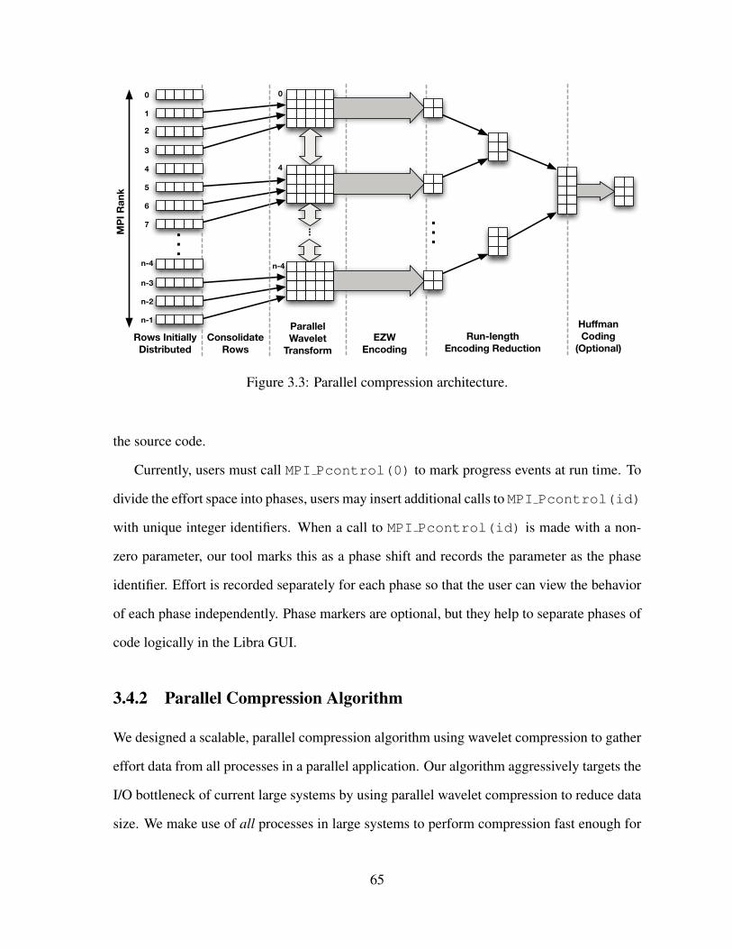
MP

I Ran

k

0

1

2

3

4

5

6

7

n-1

n-3

n-2

n-4

0

4

n-4

Rows InitiallyDistributed

ConsolidateRows

ParallelWavelet

TransformEZW

EncodingRun-length

Encoding Reduction

HuffmanCoding

(Optional)

. . . ... . .

.

Figure 3.3: Parallel compression architecture.

the source code.

Currently, users must call MPI Pcontrol(0) to mark progress events at run time. To

divide the effort space into phases, users may insert additional calls to MPI Pcontrol(id)

with unique integer identifiers. When a call to MPI Pcontrol(id) is made with a non-

zero parameter, our tool marks this as a phase shift and records the parameter as the phase

identifier. Effort is recorded separately for each phase so that the user can view the behavior

of each phase independently. Phase markers are optional, but they help to separate phases of

code logically in the Libra GUI.

3.4.2 Parallel Compression Algorithm

We designed a scalable, parallel compression algorithm using wavelet compression to gather

effort data from all processes in a parallel application. Our algorithm aggressively targets the

I/O bottleneck of current large systems by using parallel wavelet compression to reduce data

size. We make use of all processes in large systems to perform compression fast enough for

65

real-time monitoring at scale.

We base our parallel transform on that of Nielsen et al. (Nielsen and Hegland, 2000),

although our data distribution is slightly different. At the end of a trace, each process in the

distributed application has a vector of effort measurements for each effort region with one

measurement for each progress step. We can consider each of these vectors as a row in a

two-dimensional distributed matrix. For transforms within rows of this matrix, the data is

entirely local, but transforms within columns are distributed.

Our transform allocates at least D/2 (half the width of the wavelet filter) rows per pro-

cess. This ensures that only nearest-neighbor communication is necessary in the algorithm.

Further, for a level L transform, the number of rows per process should be large enough that

it can be halved recursively L times and still not shrink below D/2. To ensure this, we con-

solidate rows before performing the transform. For a system with P processes, our algorithm

regroups the distributed matrix into P/S local sets of S rows. Figure 3.3 shows how this

would look for S = 4.

On architectures such as torus or mesh networks that have dedicated network links be-

tween neighbors, this row consolidation scheme produces perfect scaling. On switched net-

works using commodity interconnects such as Infiniband, the scalability of this algorithm

will depend on the particular machine’s switching configuration and on the particular routing

scheme used (Hoefler et al., 2008).

After row consolidation, we perform the parallel transform. Our algorithm then encodes

the transformed coefficients using the Embedded Zerotree Wavelet (EZW) coding (Shapiro,

1993). We chose this encoding for two reasons. First, it parallelizes well (Ang et al., 1999;

Kutil, 2002). The data layout for Zerotree coding corresponds to the organization of trans-

formed wavelet coefficients. Encoding is entirely local to each process.

Second, it supports efficient space/accuracy trade-offs. The bits output in EZW coding

are ordered by significance. Each pass of the encoder tests wavelet coefficients against a

66

successively smaller threshold and outputs bits indicating whether the coefficients were larger

or smaller than the thresholds.

The first few passes of EZW-coded data are typically very compact, and they contain

the most significant bits of the largest coefficients in the output. We can thus obtain a good

approximation by reading a very small amount of EZW data. Examining more detailed passes

refines the quality of the approximation at a cost of higher data volume. In our framework,

the number of EZW passes is customizable, allowing the user to control this trade-off.

In the final stage of compression, we take local EZW-coded passes, run-length encode

them, and then merge the run-length encoded buffers in a parallel reduction. Each internal

node of the reduction tree receives encoded buffers from its children, splices them together

without decompressing, and sends the resulting merged buffer to its parent. Splicing is done

by joining runs of matching symbols at either end of the encoded buffer. We aggregate

this compressed data into a single buffer at the root of the reduction tree, and we Huffman-

encode (Huffman, 1952) the full buffer.

The consolidation step of our algorithm sacrifices parallelism for increased locality and

reduced communication cost. However, there are typically many effort matrices to trans-

form, and we can exploit all available parallelism by running S concurrent instances of the

compression algorithm.

Figure 3.4 gives pseudocode for our algorithm. We first split the system into S separate

sets of ranks, each with its own local communicator, using a call to MPI Comm split().

After this, the code behaves as S separate parallel encoders executing simultaneously. Each

program has P/S processes, with ranks 0 to P/S. These ranks map to modulo sets in the

entire system’s rank space.

Within each modulo set, process rank sends its first local effort vector to process 0. It

sends its next vector to process 1, and so on until S vectors have been sent. These sends con-

solidate data for S effort matrices, after which S simultaneous instances of our compression

67

DISTRIBUTE-WORK(P, S)1 comm = MPI-COMM-SPLIT(WORLD, rank % S, 0)2 v = effortV ectors.first3 while v <= effortV ectors.last4 do set← 05 while set < S and v ≤ effortV ectors.last6 do base = (rank div S) ∗ S7 if rank % S = set8 then i = 19 while i < S

10 do START-RECV-FROM(comm, base+ i)11 i← i+ 11213 else START-SEND-TO(comm, v, base)1415 set← set+ 116 v = effortV ectors.next1718 FINISH-SENDS-AND-RECEIVES(comm)19 DO-COMPRESSION(comm, localRows)

Figure 3.4: Data consolidation algorithm

68

algorithm are performed. This entire process is repeated until all effort matrices have been

encoded.

3.4.3 Trace Reconstruction

Our compression tool produces a compact representation of system-wide, temporally-ordered

load-balance data. Once stored, data can be decompressed and reconstructed for analysis or

for display in a visualization tool. The reconstruction process is simply the inverse of the

compression process. Decompression is independent for each effort region recorded at run

time, allowing focused data exploration.

The wavelet representation is particularly useful for modeling load balance because it

preserves spatial information. Because the transform records both scale- and spatial infor-

mation, when the inverse transform is applied, features represented by coefficients in the

wavelet domain are reconstructed at their original rank and progress step. Wavelets are thus

particularly useful for representing outliers, large spikes, and aperiodic data.

Our compression scheme is lossy for several reasons. The double-precision floating-point

values used in the CDF 9/7 wavelet transform introduce rounding error. The double-precision

output is then scaled and converted to 64-bit integers for EZW coding, which introduces

quantization error. Finally, the EZW output stream is truncated after a certain number of

passes, giving variable approximation error.

Our results show that the amount of error introduced by rounding and quantization is

modest. Error introduced by truncation of the EZW stream can be greater, but wavelet com-

pression and EZW coding have unique properties that make this error less problematic.

Most importantly, the wavelet transform produces approximations with very few terms,

so a large number of coefficients in the transformed data are zero or near-zero. We filter

only the less significant data by truncating an EZW stream. Higher-magnitude coefficients in

the wavelet domain correspond to more significant features in the original data. Thus, even

69

under severe compression, wavelets yield a reconstruction that is qualitatively similar to the

original data.

3.5 Experimental Results

We conducted experiments with our tool on three systems. The first is an IBM BlueGene/L

(BG/L) system with 2048 dual-core, 700 MHz PowerPC compute nodes. Each node has 1

GB RAM (512 MB per core). A 3-D torus network and two tree-strucutured networks are

available for communication among processes. We used IBM’s xlC and gcc compilers along

with IBM’s MPI implementation. In our tests, we used both of BG/L’s modes of execution:

coprocessor mode, with the second core on each node dedicated to communication; and

virtual node (VN) mode, in which both cores perform computation and communication.

The second system is a 40,960-node IBM BlueGene/P (BG/P) system. This is the suc-

cessor to BlueGene/L, and each node of this system has four PowerPC cores running at 850

MHz, for a total of 163,840 cores. Each node has 2 GB RAM. The network architecture of

BG/P is very similar to that of BG/L, but with slightly higher bandwidth.

The third system is a Linux cluster with 66 dual-processor, dual-core Intel Woodcrest

nodes. The 264 cores run at 2.6 GHz. Each node has 4 GB RAM, and Infiniband 4X is the

primary interconnect. We used the Intel compilers and OpenMPI, with Infiniband used for

inter-node communication and shared memory used for intra-node communication.

We used three well-known scientific applications for our tests, ParaDiS, Raptor, and S3D,

all of which scale to 16,000 or more processes (Louis and de Supinski, 2005). ParaDiS (Bula-

tov et al., 2004), models the dynamics of dislocation lines in crystals as a network of nodes, or

discretized points, and arms, which connect nodes in the dislocation network. ParaDiS uses

an adaptive load-balancing algorithm in which dislocations are divided into bounded regions

called domains. Each process computes on one domain, with the load balancer periodically

70

0 1 2 3 4 5 6

32 64 128 256 512 1024 2048Ove

rhea

d (%

tota

l tim

e)Number of processes

RaptorParaDiS

Figure 3.5: Tool overhead for Raptor and ParaDiS

redistributing dislocations among domains.

Raptor (Greenough et al., 2003), is an Eulerian Adaptive Mesh Refinement (AMR) code

that simulates complex fluid dynamics using the Godunov finite difference method. Like

ParaDiS, Raptor is known to have variable amounts of per-process computation. However,

whereas the underlying physics (the time evolution of dislocations) causes the imbalances in

ParaDiS, load imbalance in Raptor arises from mesh refinement.

Finally, S3D (Hawkes and Chen, 2004) is a gas-dynamics code that solves the Navier-

Stokes equations (Navier, 1822; Stokes, 1845) for turbulent combustion problems. S3D has

been shown to have imbalances in its checkpoint routines at 16,000 or more cores. We

included it in our test suite to examine I/O performance.

Instrumenting these applications required only the addition of a single function call in the

main time-step loop to denote the progress step. These loops were generally easy to locate

in the source code without prior knowledge. As mentioned, we hope to detect progress loops

automatically from MPI traces in the long term.

3.5.1 Compression Performance

To assess the performance of our data-compression library, we began by conducting scal-

ing studies using the Raptor and ParaDiS codes on our BlueGene/L system. We measured

the time consumed by our compression algorithm. This included transform, encoding, and

71

0

5

10

15

20

25

30

35

32 64 128 256 512 1024 2048 4096

Out

put T

ime

(sec

onds

)

Number of processes

RaptorRaptor, no comp.Raptor, VN mode

Raptor, no comp., VN mode

(a) Raptor on Blue Gene/L

0 10 20 30 40 50 60 70 80 90

32 64 128 256 512 1024

Out

put T

ime

(sec

onds

)

Number of processes

ParaDiSParaDiS, no comp.

(b) ParaDiS on Blue Gene/L

Figure 3.6: Compression and I/O times for 1024-timestep traces

file-write time. For comparison, we performed an identical set of runs in which we dumped

uncompressed data to disk. For these experiments, the exhaustive dump is done after the con-

solidation of rows. That is, each leaf node in our run-length encoding reduction tree dumps

its partition of the distributed matrix to a file. Thus, our exhaustive dump takes advantage of

parallel I/O if it is available.

For both applications, we ran the simulations for 1024 time-steps. During compression,

we allowed the wavelet transform to recur as deeply as possible, and we set the initial phase

of our algorithm to consolidate to 128 rows per process. We truncated the output to 4 EZW

passes. For each run, we recorded elapsed time, I/O time to write raw data, and time to

compress as well as to write compressed data.

Figure 3.5 shows tool overhead in terms of percent increase in application run time, ex-

cluding compression. For both the Raptor and ParaDiS codes, overhead was always 5% or

less compared to an uninstrumented run of the same application. This is sufficient to measure

production codes without severe perturbation.

Figure 3.6 shows the time required to write load-balance data at the end of a run, with and

without our tool. For both ParaDiS and Raptor, as system size increases, the load on the I/O

system also climbs, and the time needed to write uncompressed data increases modestly until

the I/O system is saturated. For Raptor, the I/O system saturates at around 1024 processes,

72

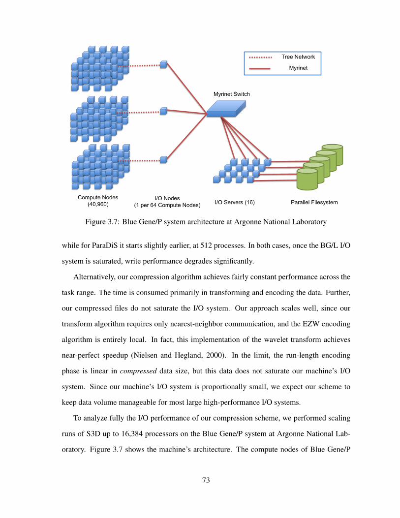
Myrinet Switch

I/O Servers (16) Parallel Filesystem Compute Nodes

(40,960) I/O Nodes

(1 per 64 Compute Nodes)

Tree Network

Myrinet

Figure 3.7: Blue Gene/P system architecture at Argonne National Laboratory

while for ParaDiS it starts slightly earlier, at 512 processes. In both cases, once the BG/L I/O

system is saturated, write performance degrades significantly.

Alternatively, our compression algorithm achieves fairly constant performance across the

task range. The time is consumed primarily in transforming and encoding the data. Further,

our compressed files do not saturate the I/O system. Our approach scales well, since our

transform algorithm requires only nearest-neighbor communication, and the EZW encoding

algorithm is entirely local. In fact, this implementation of the wavelet transform achieves

near-perfect speedup (Nielsen and Hegland, 2000). In the limit, the run-length encoding

phase is linear in compressed data size, but this data does not saturate our machine’s I/O

system. Since our machine’s I/O system is proportionally small, we expect our scheme to

keep data volume manageable for most large high-performance I/O systems.

To analyze fully the I/O performance of our compression scheme, we performed scaling

runs of S3D up to 16,384 processors on the Blue Gene/P system at Argonne National Lab-

oratory. Figure 3.7 shows the machine’s architecture. The compute nodes of Blue Gene/P

73

systems are attached to a parallel file system through I/O nodes. The system at Argonne has

64 compute nodes per I/O node, and the I/O nodes communicate with 16 file-system servers

through a Myrinet link (Boden et al., 1995). The file system in use at Argonne is IBM’s

GPFS (Schmuck and Haskin, 2002). All runs here were done by aggregating at most 512

rows to a single process.

Blue Gene/P can operate in three modes, each with slightly different I/O characteristics.

Virtual-node (VN) mode is much the same as virtual-node mode for Blue Gene/L. The four

cores on each node divide their local memory into distinct partitions, and each behaves like

a separate parallel process. In this configuration, there are 256 compute cores for every four-

core I/O node.

In dual mode, the node is split into two virtual nodes, and two shared-memory processes

share two cores each. In Symmetric MultiProcessing (SMP) mode, each compute node hosts

only one process, and that process’s threads can share its cores.

Figure 3.8 shows a detailed distribution of the time consumed by different components

of our compression algorithm for runs with S3D. Shown in the legend, the phases of our

algorithm are:

Mkdirs: Creation of output directories.

SyncKeys: Synchronize effort symbol information across all processes.

Aggregate: Consolidate distributed matrix rows onto single processes before compression.

WaveletTransform: Computation of the parallel wavelet transform.

OpenOutputFiles: Open output files for writing.

EZWStats: Global operations (global max value, etc.) required for EZW encoding.

EZWEncode: Local EZW encoding.

74

0 0.5

1 1.5

2 2.5

3 3.5

4 4.5

2048 4096 8192 16384

Mer

ge T

ime

(sec

onds

)

Processes

MkdirsSyncKeysAggregateWaveletTransformOpenOutputFilesEZWStatsEZWEncodeLocalRLERLEGatherEntropy

(a) Virtual-Node Mode

0

2

4

6

8

10

12

14

1024 2048 4096 8192 16384

Mer

ge T

ime

(sec

onds

)

Processes

MkdirsSyncKeysAggregateWaveletTransformOpenOutputFilesEZWStatsEZWEncodeLocalRLERLEGatherEntropy

(b) Dual Mode

0

5

10

15

20

25

512 1024 2048 4096 8192 16384

Mer

ge T

ime

(sec

onds

)

Processes

MkdirsSyncKeysAggregateWaveletTransformOpenOutputFilesEZWStatsEZWEncodeLocalRLERLEGatherEntropy

(c) SMP Mode

Figure 3.8: Detailed distribution of wavelet merge times for S3D on Blue Gene/P

75

LocalRLE: Local run-length encoding on result of EZW.

RLEGather: Tree-structured gather and merge of RLE-encoded data.

Entropy: Final Huffman coding on the compressed data.

In virtual-node mode (Figure 3.8a), our algorithm’s speed increases from 2048 to 16,384

processes, likely because it is able to exploit additional task parallelism and to perform a

greater number of simultaneous parallel compressions. As before, the total compression

time is between 2.5 and 5 seconds, but in all cases performance is dominated by file metadata

operations. For 2048, 4096, and 8192-process runs, most of the time is consumed by opening

output files. Making directories is the second most time-consuming task. Only a small

fraction of any run, regardless of size, is spent compressing data.

We see similar trends for dual and SMP modes (Figure 3.8b). In all cases, the actual

computational work of compression takes well under 5 seconds to complete. However, the

compression operation is dominated by file-system metadata operations. For the 1024-node

run in dual mode as well as for the 8192 and 16384-node runs in SMP mode, the time con-

sumed by metadata operations more than quadruples the running time of the compression

algorithm.

S3D is an I/O intensive application, particularly at scale. We hypothesized that our algo-

rithm was competing with S3D for I/O resources in many of the cases we observed. To assess

this, we took synthetic recorded data from S3D runs and ran our compression algorithm in

isolation, without the S3D application. We also varied from 16 to 512 the number of rows

consolidated to processes before compression to examine the trade-off between task and data

parallelism.

Results for these experiments are shown in Figures 3.9, 3.10, and 3.11. In all but one

case, the compression algorithm’s execution time remains under 10 seconds, and in the vast

majority of experiments the entire compression process takes under 5 seconds. In VN mode

76

(Figure 3.9), wavelet compression dominates the computation. Only in the 64-rows-per-

process and 256-rows-per-process cases do I/O operations contribute significantly to total

time.

In dual mode (Figure 3.10), opening output files begins to play a minor role, and making

output directories consumes a significant portion of the time for the 8,192-node run at 64

rows per process. The dual-mode jobs use the same number of processes as the VN-mode

jobs, but there are actually more I/O nodes available on dual-mode jobs than on VN-mode

jobs. The problem thus cannot be one of bandwidth. It may be that with more I/O nodes

there is more contention over the metadata server, which the results in Figure 3.11 confirm.

In SMP mode, opening output files consumes a higher percentage of total time than it did in

dual mode.

Rows per process did not have a large effect on the running time of our compression

algorithm, but for very small rows-per-process values, serial parts of the algorithm begin to

dominate. In VN and dual modes, the 16-rows-per-process run spends proportionally more

time in Huffman encoding than do any of the other runs. At 16 rows per process, we have

increased the data parallelism of our task to such a great extent that Huffman encoding has

become the limiting factor.

We can avoid this problem by increasing the number of rows consolidated. In all modes,

compression time decreases as we double the number of rows consolidated up to 256 rows

per process. However, at 512 rows per process, elapsed compression time begins to increase

again.

Tuning the rows per process thus involves parallel/sequential trade-offs between two

trends. When we decrease the rows per process, we gain parallelism but incur sequential

overhead from Huffman coding. When we increase the rows per process, we gain perfor-

mance from increased locality of transformed wavelet data, but if we increase too much, the

local wavelet transform begins to take more time due to the larger local data. On the Blue

77

Gene/P system at Argonne, our data shows that the minimal run time occurs between these

two extremes, at 256 rows per process.

3.5.2 Data Volume

In this section, we quantify the volume of data produced by our data-collection algorithm.

We characterize the degree to which users can trade accuracy for improved compression, and

we compare the total volume of data produced by our algorithm to the size of uncompressed

output. For these runs, we used a maximum of 128 rows per process, and we allowed the

wavelet transform to recur up to level 5, depending on the dimensions of the matrix to be

compressed.

As mentioned, the EZW compression algorithm allows the user to trade error and data

volume by adjusting the number of EZW passes encoded. To characterize this trade-off, we

held system size constant and varied the number of passes as we ran our tool.

Figures 3.12a and 3.12b show compressed-data sizes and compression ratios from 1024-

process, 1024-time-step runs of Raptor. The data shows that the first few EZW passes do not

consume a large amount of space when compressed. For one pass, the compression ratio is

over 10,000:1 and up to 5 passes, it is 100:1 or greater. The compressed size then increases

until around 35 passes, beyond which the total size does not increase significantly.

We next conducted runs to measure total data volume and compression ratio, varying

system size and number of EZW passes. For these runs, we ran Raptor for 1024 progress

steps and compressed data from its 16 effort regions. We also ran ParaDiS for 1024 progress

steps and compressed data from its 120 effort regions. Figure 3.13 shows these results.

Figures 3.13a and 3.13b show raw compression ratios for ParaDiS and Raptor. Record-

ing only the first pass of the EZW-encoded output, we can achieve compression ratios of

over three orders of magnitude for both codes. Recording five passes yields compression

ratios close to or above two orders of magnitude. Accordingly, Figure 3.13c shows that our

78

0 0.5

1 1.5

2 2.5

3 3.5

4 4.5

5

128256

5121024

20484096

819216384

Tim

e (n

s)

Number of Processes

(a) 16 rows per process

0

1

2

3

4

5

6

128256

5121024

20484096

819216384

Tim

e (n

s)

Number of Processes

(b) 32 rows per process

0

0.5

1

1.5

2

2.5

3

3.5

4

128256

5121024

20484096

819216384

Tim

e (n

s)

Number of Processes

(c) 64 rows per process

0

0.5

1

1.5

2

2.5

3

3.5

256512

10242048

40968192

16384

Tim

e (n

s)

Number of Processes

(d) 128 rows per process

0

0.5

1

1.5

2

2.5

5121024

20484096

819216384

Tim

e (n

s)

Number of Processes

(e) 256 rows per process

0

0.5

1

1.5

2

2.5

3

3.5

4

10242048

40968192

16384

Tim

e (n

s)

Number of Processes

(f) 512 rows per process

0

1

2

3

4

5

6

7

256512

10242048

40968192

16384

Tim

e (

ns)

Number of Processes

MkdirsSyncKeysAggregateWaveletTransformOpenOutputFilesEZWStatsEZWEncodeLocalRLERLEGatherEntropy

0

1

2

3

4

5

6

7

256512

10242048

40968192

16384

Tim

e (

ns)

Number of Processes

MkdirsSyncKeysAggregateWaveletTransformOpenOutputFilesEZWStatsEZWEncodeLocalRLERLEGatherEntropy

Figure 3.9: Stand-alone merge performance in virtual-node mode

79

0

2

4

6

8

10

12

14

128256

5121024

20484096

819216384

Tim

e (n

s)

Number of Processes

(a) 16 rows per process

0

1

2

3

4

5

6

7

128256

5121024

20484096

819216384

Tim

e (n

s)

Number of Processes

(b) 32 rows per process

0

1

2

3

4

5

6

128256

5121024

20484096

819216384

Tim

e (n

s)

Number of Processes

(c) 64 rows per process

0

1

2

3

4

5

6

7

256512

10242048

40968192

16384

Tim

e (n

s)

Number of Processes

(d) 128 rows per process

0

0.5

1

1.5

2

2.5

3

3.5

4

4.5

5121024

20484096

819216384

Tim

e (n

s)

Number of Processes

(e) 256 rows per process

0 0.5

1 1.5

2 2.5

3 3.5

4 4.5

5

10242048

40968192

16384

Tim

e (n

s)

Number of Processes

(f) 512 rows per process

0

1

2

3

4

5

6

7

256512

10242048

40968192

16384

Tim

e (

ns)

Number of Processes

MkdirsSyncKeysAggregateWaveletTransformOpenOutputFilesEZWStatsEZWEncodeLocalRLERLEGatherEntropy

0

1

2

3

4

5

6

7

256512

10242048

40968192

16384

Tim

e (

ns)

Number of Processes

MkdirsSyncKeysAggregateWaveletTransformOpenOutputFilesEZWStatsEZWEncodeLocalRLERLEGatherEntropy

Figure 3.10: Stand-alone merge performance in dual mode

80

0

1

2

3

4

5

6

128256

5121024

20484096

8192

Tim

e (n

s)

Number of Processes

(a) 16 rows per process

0

1

2

3

4

5

6

7

8

9

128256

5121024

20484096

8192

Tim

e (n

s)

Number of Processes

(b) 32 rows per process

0 1 2 3 4 5 6 7 8 9

10

128256

5121024

20484096

8192

Tim

e (n

s)

Number of Processes

(c) 64 rows per process

0

1

2

3

4

5

6

256512

10242048

40968192

Tim

e (n

s)

Number of Processes

(d) 128 rows per process

0

1

2

3

4

5

6

5121024

20484096

8192

Tim

e (n

s)

Number of Processes

(e) 256 rows per process

0 1 2 3 4 5 6 7 8 9

10

10242048

40968192

Tim

e (n

s)

Number of Processes

(f) 512 rows per process

0

1

2

3

4

5

6

7

256512

10242048

40968192

16384

Tim

e (

ns)

Number of Processes

MkdirsSyncKeysAggregateWaveletTransformOpenOutputFilesEZWStatsEZWEncodeLocalRLERLEGatherEntropy

0

1

2

3

4

5

6

7

256512

10242048

40968192

16384

Tim

e (

ns)

Number of Processes

MkdirsSyncKeysAggregateWaveletTransformOpenOutputFilesEZWStatsEZWEncodeLocalRLERLEGatherEntropy

Figure 3.11: Stand-alone merge performance in SMP mode

81

1000 10000

100000 1e+06 1e+07 1e+08 1e+09

0 8 16 24 32 40 48 56 64

Byte

s

EZW Passes

RaptorParaDiS

(a) Compressed size vs. encoded passes

0.1 1

10 100

1000 10000

100000

0 8 16 24 32 40 48 56 64

Com

pres

sion

Rat

io

EZW Passes

RaptorParaDiS

(b) Compression ratio vs. encoded passes

Figure 3.12: Varying EZW passes

1

10

100

1000

10000

100000

1e+06

64 128 256 512 1024 2048 4096

Com

pres

sion

Rat

io (:

1)

Processes

(a) Compression ratio vs. processes (Raptor)

1

10

100

1000

10000

100000

1e+06

32 64 128 256 512 1024

Com

pres

sion

Rat

io (:

1)

Processes

(b) Compression ratio vs. processes (ParaDiS)

1000

10000

100000

1e+06

1e+07

1e+08

1e+09

64 128 256 512 1024 2048 4096

Tota

l dat

a si

ze (b

ytes

)

Processes

(c) Total compressed size vs. processes (Raptor)

1000

10000

100000

1e+06

1e+07

1e+08

1e+09

32 64 128 256 512 1024

Tota

l dat

a si

ze (b

ytes

)

Processes

(d) Total compressed size vs. processes (ParaDiS)

1

1e+20

1e+40

1e+60

1e+80

1e+100

32 64 128 256 512 1024

Co

mp

ressio

n R

atio

(:1

)

Processes

1 pass2 pass3 pass4 pass5 pass7 pass

10 passUncomp.

0 5 10 15 20 25 30 35 40 45 50 55 60 65 70 75 80 85 90 95 100 105 110 115 120 125 130 135 140 145 150 155 160 165 170 175 180 185 190 195 200 205 210 215 220 225 230 235 240 245 250 255 260 265 270 275 280 285 290 295 300 305 310 315 320 325 330 335 340 345 350 355 360 365 370 375 380 385 390 395 400 405 410 415 420 425 430 435 440 445 450 455 460 465 470 475 480 485 490 495 500

64 128 256 512 1024 2048 4096

No

rma

lize

d R

MS

Err

or

(%)

Processes

1 pass2 pass3 pass4 pass5 pass7 pass

10 pass64 pass

0 5 10 15 20 25 30 35 40 45 50 55 60 65 70 75 80 85 90 95 100 105 110 115 120 125 130 135 140 145 150 155 160 165 170 175 180 185 190 195 200 205 210 215 220 225 230 235 240 245 250 255 260 265 270 275 280 285 290 295 300 305 310 315 320 325 330 335 340 345 350 355 360 365 370 375 380 385 390 395 400 405 410 415 420 425 430 435 440 445 450 455 460 465 470 475 480 485 490 495 500

64 128 256 512 1024 2048 4096

No

rma

lize

d R

MS

Err

or

(%)

Processes

1 pass2 pass3 pass4 pass5 pass7 pass

10 pass64 pass

0 5 10 15 20 25 30 35 40 45 50 55 60 65 70 75 80 85 90 95 100 105 110 115 120 125 130 135 140 145 150 155 160 165 170 175 180 185 190 195 200 205 210 215 220 225 230 235 240 245 250 255 260 265 270 275 280 285 290 295 300 305 310 315 320 325 330 335 340 345 350 355 360 365 370 375 380 385 390 395 400 405 410 415 420 425 430 435 440 445 450 455 460 465 470 475 480 485 490 495 500

64 128 256 512 1024 2048 4096

No

rma

lize

d R

MS

Err

or

(%)

Processes

1 pass2 pass3 pass4 pass5 pass7 pass

10 pass64 pass

0 5 10 15 20 25 30 35 40 45 50 55 60 65 70 75 80 85 90 95 100 105 110 115 120 125 130 135 140 145 150 155 160 165 170 175 180 185 190 195 200 205 210 215 220 225 230 235 240 245 250 255 260 265 270 275 280 285 290 295 300 305 310 315 320 325 330 335 340 345 350 355 360 365 370 375 380 385 390 395 400 405 410 415 420 425 430 435 440 445 450 455 460 465 470 475 480 485 490 495 500

64 128 256 512 1024 2048 4096

No

rma

lize

d R

MS

Err

or

(%)

Processes

1 pass2 pass3 pass4 pass5 pass7 pass

10 pass64 pass

0 5 10 15 20 25 30 35 40 45 50 55 60 65 70 75 80 85 90 95 100 105 110 115 120 125 130 135 140 145 150 155 160 165 170 175 180 185 190 195 200 205 210 215 220 225 230 235 240 245 250 255 260 265 270 275 280 285 290 295 300 305 310 315 320 325 330 335 340 345 350 355 360 365 370 375 380 385 390 395 400 405 410 415 420 425 430 435 440 445 450 455 460 465 470 475 480 485 490 495 500

64 128 256 512 1024 2048 4096

No

rma

lize

d R

MS

Err

or

(%)

Processes

1 pass2 pass3 pass4 pass5 pass7 pass

10 pass64 pass

0 5 10 15 20 25 30 35 40 45 50 55 60 65 70 75 80 85 90 95 100 105 110 115 120 125 130 135 140 145 150 155 160 165 170 175 180 185 190 195 200 205 210 215 220 225 230 235 240 245 250 255 260 265 270 275 280 285 290 295 300 305 310 315 320 325 330 335 340 345 350 355 360 365 370 375 380 385 390 395 400 405 410 415 420 425 430 435 440 445 450 455 460 465 470 475 480 485 490 495 500

64 128 256 512 1024 2048 4096

No

rma

lize

d R

MS

Err

or

(%)

Processes

1 pass2 pass3 pass4 pass5 pass7 pass

10 pass64 pass

0 5 10 15 20 25 30 35 40 45 50 55 60 65 70 75 80 85 90 95 100 105 110 115 120 125 130 135 140 145 150 155 160 165 170 175 180 185 190 195 200 205 210 215 220 225 230 235 240 245 250 255 260 265 270 275 280 285 290 295 300 305 310 315 320 325 330 335 340 345 350 355 360 365 370 375 380 385 390 395 400 405 410 415 420 425 430 435 440 445 450 455 460 465 470 475 480 485 490 495 500

64 128 256 512 1024 2048 4096

No

rma

lize

d R

MS

Err

or

(%)

Processes

1 pass2 pass3 pass4 pass5 pass7 pass

10 pass64 pass

Figure 3.13: Total data volume and compression ratios

82

Figure 3.14: Embedding of the MPI rank space in S3D’s process topology

compressed representation is always well below the size of the uncompressed data.

As discussed in §3.1, the compute-to-I/O ratio in modern supercomputers is high. Com-

pression ratios in the range of 100:1-1000:1 reduce this gap and allow system-wide data

collection without perturbation. Figure 3.6, e.g., clearly shows that our algorithm is bounded

only by the local time needed to transform and to encode, while dumping exhaustive data is

bound by the capacity of the I/O system.

3.6 Exploiting Application Topology

Our compression algorithm uses the MPI rank order for its wavelet-transform topology. Since

this is a one-dimensional space, it does not always map directly to the model topology of

applications, which means that the locality of data in the wavelet transform does not map

directly to any inherent locality that application-model data may have.

Figure 3.14 shows the one-dimensional rank embedding used by S3D. S3D’s model

topology is a three-dimensional grid of processes, which correspond to spatial dimensions

in the physical simulation. MPI ranks are row-major within XY planes in the grid, with the

origin of each XY plane connected to the upper right corner of its successor.

83

0 1e+06 2e+06 3e+06 4e+06 5e+06 6e+06 7e+06 8e+06

1024 2048 4096 8192 16384

Dat

a Vo

lum

e (B

ytes

)

Number of Processors

SMP mode, standard topologySMP mode, alternate topology

VN mode, standard topologyVN mode, alternate topology

(a) Data volume

-1

-0.5

0

0.5

1

1.5

2

2.5

512 1024 2048 4096 8192 16384

Perc

ent c

hang

e

Number of Processors

SMP modeVN mode

(b) Percent change with alternate topology

Figure 3.15: S3D compressed data volume with standard and alternative topologies

Prior work has shown that the performance characteristics in three-dimensional simula-

tions like S3D are related to the process’s neighbor count (Ahn and Vetter, 2002). Corner

processes in this space have fewer neighbors (3) than edge processes (4). Edge processes

likewise have fewer neighbors than face processes (5). Interior processes have 6 neighbors.

To assess how the MPI-rank embedding affects compression quality, we conducted runs

of S3D that compressed the same data with S3D’s default MPI-rank embedding and with an

alternate embedding intended to maximize local similarity of performance in the MPI-rank

space. Our alternate embedding orders processes by their neighbor count: first corners, then

edges, then faces, then finally interior processes, in ascending order within the MPI-rank

space.

For both topologies, we consolidated 128 rows per process and performed a level-7

wavelet transform before EZW encoding. We recorded only the first five EZW passes to

disk. We ran these experiments on Blue Gene/P with up to 16,384 processes, both with one

process per node (SMP mode) and with four processes per node (VN mode).

Figure 3.15a shows the total compressed data volume for both approaches, and Figure

3.15b shows the percent change in data volume for S3D’s topology versus ours. For all

system sizes, the total compressed data volume in SMP mode and VN mode is nearly the

same. However, the topology used makes a small difference. From 512-4096 processes, and

84

1e-10

1e-08

1e-06

0.0001

0.01

1

100

0 8 16 24 32 40 48 56 64

Nor

mal

ized

RM

S Er

ror (

%)

EZW Passes

Quartiles

(a) Raptor

1e-10

1e-08

1e-06

0.0001

0.01

1

100

0 8 16 24 32 40 48 56 64

Nor

mal

ized

RM

S Er

ror (

%)

EZW Passes

Quartiles

(b) ParaDiS

Figure 3.16: Error vs. encoded EZW passes

with 16,384 processes, compressed data with our topology is half a percent to 1.5% larger

than with the standard topology.

The only size for which compression with our topology was more efficient than compres-

sion with the standard topology was 8,192 processors. However, our topology only reduces

data volume by half a percent in SMP mode, and in VN mode there is almost no difference

in size. Interestingly, our compression is twice as efficient with S3D data from 8,192 process

run as it is for data from 4,096 processes.

3.6.1 Reconstruction Error

There are three sources of error in our compression algorithm: rounding error in the CDF 9/7

wavelet transform, quantization error in the encoding process, and EZW pass thresholding.

The first two sources are unavoidable, but they contribute only modestly to the total error. The

third can be adjusted to trade space and accuracy. Obviously, we cannot afford to discard too

much data, as severe error would hinder the characterization of effort.

We characterize error in our compression algorithm in two ways. In this section, we

provide a quantitative discussion of error in our algorithm. In the next section, we discuss

the qualitative error of our method by comparing compressed data from our tool to exact

data.

85

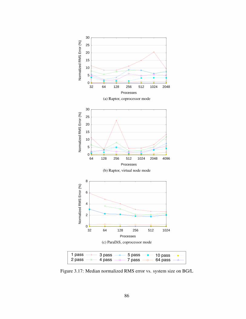
0

5

10

15

20

25

30

32 64 128 256 512 1024 2048

Nor

mal

ized

RM

S Er

ror (

%)

Processes

(a) Raptor, coprocessor mode

0

5

10

15

20

25

30

64 128 256 512 1024 2048 4096

Nor

mal

ized

RM

S Er

ror (

%)

Processes

(b) Raptor, virtual node mode

0

2

4

6

8

32 64 128 256 512 1024

Nor

mal

ized

RM

S Er

ror (

%)

Processes

(c) ParaDiS, coprocessor mode

0 5 10 15 20 25 30 35 40 45 50 55 60 65 70 75 80 85 90 95 100 105 110 115 120 125 130 135 140 145 150 155 160 165 170 175 180 185 190 195 200 205 210 215 220 225 230 235 240 245 250 255 260 265 270 275 280 285 290 295 300 305 310 315 320 325 330 335 340 345 350 355 360 365 370 375 380 385 390 395 400 405 410 415 420 425 430 435 440 445 450 455 460 465 470 475 480 485 490 495 500

64 128 256 512 1024 2048 4096

Norm

aliz

ed R

MS

Err

or

(%)

Processes

1 pass2 pass3 pass4 pass5 pass7 pass

10 pass64 pass

0 5 10 15 20 25 30 35 40 45 50 55 60 65 70 75 80 85 90 95 100 105 110 115 120 125 130 135 140 145 150 155 160 165 170 175 180 185 190 195 200 205 210 215 220 225 230 235 240 245 250 255 260 265 270 275 280 285 290 295 300 305 310 315 320 325 330 335 340 345 350 355 360 365 370 375 380 385 390 395 400 405 410 415 420 425 430 435 440 445 450 455 460 465 470 475 480 485 490 495 500

64 128 256 512 1024 2048 4096

Norm

aliz

ed R

MS

Err

or

(%)

Processes

1 pass2 pass3 pass4 pass5 pass7 pass

10 pass64 pass

0 5 10 15 20 25 30 35 40 45 50 55 60 65 70 75 80 85 90 95 100 105 110 115 120 125 130 135 140 145 150 155 160 165 170 175 180 185 190 195 200 205 210 215 220 225 230 235 240 245 250 255 260 265 270 275 280 285 290 295 300 305 310 315 320 325 330 335 340 345 350 355 360 365 370 375 380 385 390 395 400 405 410 415 420 425 430 435 440 445 450 455 460 465 470 475 480 485 490 495 500

64 128 256 512 1024 2048 4096

Norm

aliz

ed R

MS

Err

or

(%)

Processes

1 pass2 pass3 pass4 pass5 pass7 pass

10 pass64 pass

0 5 10 15 20 25 30 35 40 45 50 55 60 65 70 75 80 85 90 95 100 105 110 115 120 125 130 135 140 145 150 155 160 165 170 175 180 185 190 195 200 205 210 215 220 225 230 235 240 245 250 255 260 265 270 275 280 285 290 295 300 305 310 315 320 325 330 335 340 345 350 355 360 365 370 375 380 385 390 395 400 405 410 415 420 425 430 435 440 445 450 455 460 465 470 475 480 485 490 495 500

64 128 256 512 1024 2048 4096

Norm

aliz

ed R

MS

Err

or

(%)

Processes

1 pass2 pass3 pass4 pass5 pass7 pass

10 pass64 pass

0 5 10 15 20 25 30 35 40 45 50 55 60 65 70 75 80 85 90 95 100 105 110 115 120 125 130 135 140 145 150 155 160 165 170 175 180 185 190 195 200 205 210 215 220 225 230 235 240 245 250 255 260 265 270 275 280 285 290 295 300 305 310 315 320 325 330 335 340 345 350 355 360 365 370 375 380 385 390 395 400 405 410 415 420 425 430 435 440 445 450 455 460 465 470 475 480 485 490 495 500

64 128 256 512 1024 2048 4096

Norm

aliz

ed R

MS

Err

or

(%)

Processes

1 pass2 pass3 pass4 pass5 pass7 pass

10 pass64 pass

0 5 10 15 20 25 30 35 40 45 50 55 60 65 70 75 80 85 90 95 100 105 110 115 120 125 130 135 140 145 150 155 160 165 170 175 180 185 190 195 200 205 210 215 220 225 230 235 240 245 250 255 260 265 270 275 280 285 290 295 300 305 310 315 320 325 330 335 340 345 350 355 360 365 370 375 380 385 390 395 400 405 410 415 420 425 430 435 440 445 450 455 460 465 470 475 480 485 490 495 500

64 128 256 512 1024 2048 4096

Norm

aliz

ed R

MS

Err

or

(%)

Processes

1 pass2 pass3 pass4 pass5 pass7 pass

10 pass64 pass

0 5 10 15 20 25 30 35 40 45 50 55 60 65 70 75 80 85 90 95 100 105 110 115 120 125 130 135 140 145 150 155 160 165 170 175 180 185 190 195 200 205 210 215 220 225 230 235 240 245 250 255 260 265 270 275 280 285 290 295 300 305 310 315 320 325 330 335 340 345 350 355 360 365 370 375 380 385 390 395 400 405 410 415 420 425 430 435 440 445 450 455 460 465 470 475 480 485 490 495 500

64 128 256 512 1024 2048 4096

Norm

aliz

ed R

MS

Err

or

(%)

Processes

1 pass2 pass3 pass4 pass5 pass7 pass

10 pass64 pass

0 5 10 15 20 25 30 35 40 45 50 55 60 65 70 75 80 85 90 95 100 105 110 115 120 125 130 135 140 145 150 155 160 165 170 175 180 185 190 195 200 205 210 215 220 225 230 235 240 245 250 255 260 265 270 275 280 285 290 295 300 305 310 315 320 325 330 335 340 345 350 355 360 365 370 375 380 385 390 395 400 405 410 415 420 425 430 435 440 445 450 455 460 465 470 475 480 485 490 495 500

64 128 256 512 1024 2048 4096

Norm

aliz

ed R

MS

Err

or

(%)

Processes

1 pass2 pass3 pass4 pass5 pass7 pass

10 pass64 pass

Figure 3.17: Median normalized RMS error vs. system size on BG/L

86

MPI RankProgress

0 0

128256

Eff

ort

(ns

x 10

6 )

0

2

(a) 1 pass

MPI RankProgress

0 0

128256

Eff

ort

(ns

x 10

6 )

0

2

(b) 2 passes

MPI RankProgress

0 0

128256

Eff

ort

(ns

x 10

6 )

0

2

(c) 3 passes

MPI RankProgress

0 0

128256

Eff

ort

(ns

x 10

6 )

0

2

(d) 4 passes

MPI RankProgress

0 0

128256

Eff

ort

(ns

x 10

6 )

0

2

(e) 5 passes

MPI RankProgress

0 0

128256

Eff

ort

(ns

x 10

6 )

0

2

(f) 7 passes

MPI RankProgress

0 0

128256

Eff

ort

(ns

x 10

6 )

0

2

(g) 15 passes

MPI RankProgress

0 0

128256

Eff

ort

(ns

x 10

6 )

0

2

(h) Exact

Figure 3.18: Progressively refined reconstructions of the remesh phase in ParaDiS

87

We use root mean-squared (RMS) error, normalized to the range of values observed, to

evaluate reconstruction error quantitatively. For an m by n effort matrix E and its recon-

struction R, the normalized RMS error is:

nrmse(E,R) =1

max(E)−min(E)

√√√√∑ij

(Rij − Eij)2

mn(3.2)

where max(E) and min(E) are the maximum and minimum values observed in the exact

data. We normalize the error to compare the results across applications, job sizes, and input

sets.

We conducted 1024-process, 1024-progress step runs of Raptor and ParaDiS, varying

the number of EZW passes output to the compressed files. Figure 3.16 shows the normal-

ized RMS error for each of these runs. We use boxplots to show how error varies with the

characteristics of different effort regions.

For Raptor, there are 16 effort regions, and for ParaDiS, there are 120. Our box plots show

rectangles from the top to bottom quartile of compression ratios, with whiskers extending to

the maximum and minimum values. The median value is denoted by a black tick inside the

box.

For Raptor (Figure 3.16a) the median error decreases from around 10% for a 1-pass run

to near zero (8.8 × 10−6%) for a full 64-pass run. For the first few passes, there is a wide

range from 1% to 25%. After four passes, the median error is 4% and only the top quartile of

error values exceeds 10%. By seven passes, median error is less than 1% and no error value

exceeds 10%.

Comparing these error values with the corresponding compression ratios shown in Figure

3.12b, median 4% measurement error can be achieved with compression ratios of over 500:1.

The ParaDiS results in Figure 3.16b are similar to those from Raptor. Median error starts

above 10% with a wide spread, but it drops quickly. Again, at seven passes error is less

88

than 1% and by 30 passes there is little loss of accuracy. Across the board, median error for

ParaDiS is slightly lower than that for Raptor.

To assess whether reconstruction error remains stable as system size increases, we con-

ducted scaling runs of Raptor and ParaDiS, varying system size and number of EZW passes.

Again, we recorded exhaustive data along with compressed data at the end of each run, and

we compared the two to obtain error values. Figure 3.17 shows the median normalized RMS

error for these runs. For ParaDiS, error decreases as we scale the system size up, and it sta-

bilizes near 1024 processes. The decrease in error is likely due to use of strong scaling in

our ParaDiS runs. As the number of processes increases, the amount of work per process

shrinks, and more processes are left idle. Compression improves as the number of similar

idle processes grows.

Our scaling runs of Raptor show more variable error, as we used a data set with heavier

load. There are spikes in median error for the 256- and 4096- process runs in virtual node

mode, as well as the 1024-process run of Raptor in coprocessor mode.

In all cases, the spikes are only significant for runs with one EZW pass. In these cases, the

median error can jump above 20%. However, the median error is below 10% for all runs with

three or more EZW passes, and we showed previously that a truncating to a modest number

of EZW passes does not incur excessive costs in terms of data volume or compression time.

Median error is lower than 5% with five passes for both applications, regardless of system

size.

3.6.2 Qualitative Evaluation of Reconstruction

In §3.3 we reviewed the most useful properties of wavelet transforms for reconstructing load-

balance information. Specifically, we noted that the wavelet transform yields a multi-scale

representation of its input data, and that it preserves local features. For qualitative evaluation

of our approach, we conducted a small run of ParaDiS for 256 time steps with 128 processes

89

MPI RankProgress

0 0

128256

Eff

ort

(ns

x 10

4 )

0

4

(a) Force Computation, Exact

MPI RankProgress

0 0

128256

Eff

ort

(ns

x 10

4 )

0

4

(b) Force Computation, Reconstructed

MPI RankProgress

0 0

128256

Eff

ort

(ns

x 10

6 )

0

9

(c) Collision computation, Exact

MPI RankProgress

0 0

128256

Eff

ort

(ns

x 10

6 )

0

9

(d) Collision computation, Reconstructed

MPI RankProgress

0 0

128256

Eff

ort

(ns

x 10

7 )

0

8

(e) Checkpoint, Exact

MPI RankProgress

0 0

128256

Eff

ort

(ns

x 10

7 )

0

8

(f) Checkpoint, Reconstructed

MPI RankProgress

0 0

128256

Eff

ort

(ns

x 10

6 )

0

2

(g) Remesh, Exact

MPI RankProgress

0 0

128256

Eff

ort

(ns

x 10

6 )

0

2

(h) Remesh, Reconstructed

Figure 3.19: Exact and reconstructed effort plots for phases of ParaDiS

90

on a commodity Linux cluster. We plotted reconstructed effort for several phases of the

application’s execution. To illustrate the quality of reconstruction, we also recorded exact

data for comparison. To illustrate load imbalance, we used a data set that was small enough

that load could not be allocated evenly across all processes.

Figure 3.18 shows reconstructions of the effort for ParaDiS’s remesh phase for varying

EZW pass counts. As discussed in §3.6.1, lower numbers of passes correspond to higher

levels of compression and larger error, which the figure reflects. With one EZW pass, the

plot only crudely approximates the shape of the exact data, and the entire effort plot is shifted

down. With two passes, the plot, now at approximately the right position, captures the most

significant peaks although finer details of the exact reconstruction are not present. After

only four passes, the shape of the reconstruction is very close to that of the exact data, and

small load spikes in the first few iterations have appeared. By 15 passes, the reconstruction

essentially matches the exact data.

Figure 3.19 shows exact and reconstructed effort for four phases of ParaDiS. In all plots,

vertical axis shows effort in elapsed nanoseconds. The dimensions of the surface are process

identifiers (from 0-127) and progress (steps 0-255).

Figures 3.19a and 3.19b show the load distribution for ParaDiS’s force computation. This

phase, which is the most computationally intense region of ParaDiS, calculates forces on

crystal dislocations. The reconstruction very closely matches the original data. Both clearly

have two sets of processors where load is concentrated for the duration of the run. These

sets correspond to the processes to which most of the initial data set was allocated. The

reconstruction preserves the initial peaks as well as finer details in the ridges that follow for

both process sets.

Figures 3.19c and 3.19d show the effort for collision computation in ParaDiS. We selected

this phase because it illustrates the preservation of transient load. The collision computation

is data-dependent in that it occurs only when simulated dislocations collide with one another.

91

Our data has numerous spikes in the load and our compression framework preserves the

larger ones. Noisy high-frequency data at the base of the spikes is lost with only four EZW

passes, but could be preserved using more passes.

Figures 3.19e and 3.19f show the load in the checkpoint phase of ParaDiS. For these runs,

checkpoints were written to disk every 100 time steps, and the load on all processes increases

at this point. The two system-wide load spikes are clearly visible in the reconstruction at the

same time steps at which they occurred in the original execution. Although the tops of the

spikes are slightly distorted, the reconstruction is almost identical to the original data.

The remesh phase of ParaDiS, shown in Figures 3.19g and 3.19h, involves uneven load

across processors, as well as variable-frequency data. With only four passes, our technique is

unable to capture all detail, but major features are still present. The reconstruction preserves

three spikes in the initial iteration as well as the six ridges that run through all time steps.

Though not exact, this reconstruction is more than sufficient for characterizing system-wide

load distribution and for guiding optimization. And, as Figure 3.18 shows, we can increase

the number of passes stored at a slight cost in compression if more detail is required.

3.7 Summary

In this chapter, we presented a novel approach to system-wide monitoring that achieves sev-

eral orders of magnitude of data reduction and sublinear merge times, regardless of system

size. We introduced a model for high-level load semantics in SPMD applications. Using

aggressive compression techniques from signal processing and image analysis, our approach

can reduce and aggregate distributed load data to accommodate significant I/O bottlenecks.

Additionally, our approach achieves very low error rates and high speed, even at the highest

levels of compression.

We demonstrated our novel load-balance analysis framework with three actively used

92

full applications with dynamic behavior: Raptor and ParaDiS. Our framework is capable of

efficiently handling both applications and captures information that has yielded insight into

the evolution of load-balance problems, as demonstrated in our qualitative study of ParaDiS.

Additionally, our evaluation showed that even with timing and rank information the size

of the data files grows slowly with the number of processors and, hence, allows detailed

measurement even at large scales. Further, we demonstrated that our framework preserves

significant qualitative features of compressed data, even for very small compressed file sizes.

93

Chapter 4

Trace Sampling

4.1 Introduction

The previous chapter detailed an approach for lossy compression of load-balance data using

techniques adapted from signal processing and imaging to transform and reduce performance

data. In this chapter we introduce a second technique for scalable, system-wide data collec-

tion that uses statistical sampling to reduce data volume.

Sampling has been used historically to estimate properties of large populations for sur-

veys and opinion polls (U.S. Census Bureau, 2009; Gallup Organization, 2009; Cochran,

1977; Schaeffer et al., 2006). Unlike wavelet compression, which performs signal analysis

to reduce a data set to a set of approximation coefficents, sampling randomly selects repre-

sentative values from a data set according to statistical parameters. We demonstrate here that

it can be applied to performance traces to reduce data volume.

Recall that in large systems, full-application event traces can grow to unmanageable sizes.

Peak I/O throughput of the BlueGene/L system at Lawrence Livermore National Laboratory

is around 42 GB/s (Ross et al., 2006)1. A full trace from all of its 212,992 processors could

easily saturate this pathway, perturbing measurements and making the recorded trace useless.

1Ross puts the throughput at 25 GB/s, but this was measured before Blue Gene/L was upgraded from131,072 cores. For consistency, we have scaled the throughput proportionally with the system size.

Fortunately, Amdahl’s law dictates that scalable applications exhibit extremely regular

behavior. A scalable performance-monitoring system could exploit such regularity to remove

redundancies in collected data so that its outputs would not depend on total system size. An

analyst using such a system could collect just enough performance data to assess application

performance, and no more.

The difficulty of such an approach lies in deciding just how much data is enough for

performance analysis. In wavelet compression, we value thresholds by truncating an EZW

stream, but we still must collect values from all processes at the first level of the transform.

Using sampling, we instead pick a random subset of processes from the population, and we

sample only these processes to estimate properties of the system as a whole.

It has been shown using simulation and ex post facto experiments (Mendes and Reed,

2004) that statistical sampling is a promising approach to the data-reduction problem. We

can use it to estimate accurately the global properties of a population of processes without

collecting data from all of them. Sampling is particularly well suited to large systems, be-

cause the sample size needed to measure a set of processes scales sub-linearly with the size of

the set. For data with fixed variance, the sample size is constant in the limit. Thus sampling

very large populations of processes is proportionally much less costly than measuring small

ones.

We extend existing work with techniques for on-line, adaptively sampled event tracing

of arbitrary performance metrics gathered using on-node instrumentation. We dynamically

collect summary data and use it to tune the sample size as a run progresses. We also present

techniques for subdividing, or stratifying, a population into independently sampled behav-

ioral equivalence classes. Stratification can provide insight into the workings of an appli-

cation, as it gives the analyst a rough classification of the behavior of running processes.

If the behavior within each stratum is homogeneous, the overall cost of monitoring is re-

duced. These techniques are implemented in the Adaptive Monitoring and Profiling Library

95

(AMPL), a library for Libra which can be linked with instrumented scientific applications.

The remainder of this chapter is organized as follows. In §4.2, we detail statistical sam-

pling theory, emphasizing its fitness for performance monitoring. We describe the architec-

ture and implementation of AMPL in §4.3. An experimental validation of AMPL is given in

§4.4. We summarize of our research contributions in §4.5.

4.2 Statistical Sampling Theory

Statistical sampling has long been used in surveys and opinion polls to estimate general

characteristics of populations by observing the responses of only a small subset, or sample,

of the total population. Here, we review the basic principles of sampling theory, and we

present their application to scalable performance monitoring. We also discuss how samples

can be stratified to reduce sampling cost further.

4.2.1 Estimating Mean Values

Given a set of population elements Y , sampling theory estimates the mean using only a small

sample of the total population. For sample elements, y1, y2, ..., yn, the sample mean y is an

estimator of the population mean Y . We would like to ensure that the value of y is within a

certain error bound d of Y with some confidence. If we denote the risk of not falling within

the error bound as α, then the confidence is 1− α, yielding

Pr(|Y − y| > d) ≤ α. (4.1)

Stated differently, zα standard deviations of the estimator should fall within the error bound:

zα√V ar(y) ≤ d, (4.2)

96

100

101

102

103

104

105

106

107

108

109

1010

100

101

102

103

104

105

Population Size

Min

imu

m S

am

ple

Siz

e

Confidence .90, Error .08

Confidence .95, Error .05

Confidence .98, Error .03

Confidence .99, Error .01

Figure 4.1: Minimum sample size vs. population size

where zα is the normal confidence interval computed from the confidence bound 1−α. Given

the variance of an estimator for the population mean, we can solve this inequality to obtain

a minimum sample size, n, that will satisfy the constraints zα and d. For a simple random

sample, we have

n ≥ N

[1 +N

(d

zαS

)2]−1

(4.3)

where S is the standard deviation of the population, and N is the total population size.

The estimation of mean values is described elsewhere (Schaeffer et al., 2006; Mendes

and Reed, 2004), so we omit further elementary derivations. However, two aspects of (4.3)

warrant emphasis. First, (4.3) implies that the minimum cost of monitoring a population

depends on its variance. Given the same confidence and error bounds. a population with high

variance requires more sampled elements than a population with low variance. Intuitively,

highly regular SPMD codes with limited data-dependent behavior will benefit more from

sampling than will more irregular, dynamic codes.

Second, as N increases, n approaches (zαS/d)2, and the relative sampling cost n/N

97

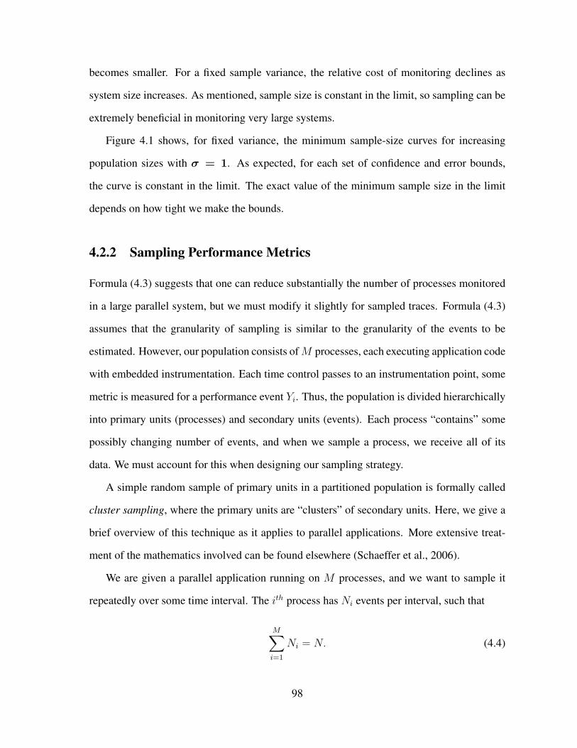
becomes smaller. For a fixed sample variance, the relative cost of monitoring declines as

system size increases. As mentioned, sample size is constant in the limit, so sampling can be

extremely beneficial in monitoring very large systems.

Figure 4.1 shows, for fixed variance, the minimum sample-size curves for increasing

population sizes with σ = 1. As expected, for each set of confidence and error bounds,

the curve is constant in the limit. The exact value of the minimum sample size in the limit

depends on how tight we make the bounds.

4.2.2 Sampling Performance Metrics

Formula (4.3) suggests that one can reduce substantially the number of processes monitored

in a large parallel system, but we must modify it slightly for sampled traces. Formula (4.3)

assumes that the granularity of sampling is similar to the granularity of the events to be

estimated. However, our population consists ofM processes, each executing application code

with embedded instrumentation. Each time control passes to an instrumentation point, some

metric is measured for a performance event Yi. Thus, the population is divided hierarchically

into primary units (processes) and secondary units (events). Each process “contains” some

possibly changing number of events, and when we sample a process, we receive all of its

data. We must account for this when designing our sampling strategy.

A simple random sample of primary units in a partitioned population is formally called

cluster sampling, where the primary units are “clusters” of secondary units. Here, we give a

brief overview of this technique as it applies to parallel applications. More extensive treat-

ment of the mathematics involved can be found elsewhere (Schaeffer et al., 2006).

We are given a parallel application running on M processes, and we want to sample it

repeatedly over some time interval. The ith process has Ni events per interval, such that

M∑i=1

Ni = N. (4.4)

98

Events on each process are Yij , where i = 1, 2, ...,M ; j = 1, 2, ..., Ni. The population mean

Y is simply the mean over the values of all events:

Y =1

N

M∑i=1

N∑j=1

Yij. (4.5)

We wish to estimate Y using a random sample ofm processes. The counts of events collected

from the sampled processes are referred to as ni. Y can be estimated from the sample values

with the cluster sample mean:

yc =

∑mi=1 yiT∑mi=1 ni

, (4.6)

where yiT is the total of all sample values collected from the ith process. The cluster mean yc

is then simply the sum of all sample values divided by the number of events sampled.

Given that yc is an effective estimator for Y , one must choose a suitable sample size to

ensure statistical confidence in the estimator. To compute this, we need the variance, given

by:

V ar(yc) =M −mMmN2

s2r, s2

r =

∑mi=1(yiT − ycni)2

m− 1(4.7)

where N is the average number of events for each process in the primary population, and s2r

is an estimator for the secondary population variance S2. We can use V ar(yc) in (4.2) and

obtain an equation for sample size as follows:

m =Ms2

r

N2V 2 + s2r

, V =

(d

zα

)2

(4.8)

The only remaining unknown is N , the number of unique events. For this, we can use a

straightforward estimator, N ≈ Mn/m. We can now use equation (4.8) for adaptive sam-

pling. Given an estimate for the variance of the event population, we can calculate approxi-

mately the size, m, of our next sample.

99

4.2.3 Stratified Sampling

Parallel applications often have behavioral equivalence classes among their processes, which

is reflected in performance data about the application. For example, if process zero of an

application reads input data, manages checkpoints and writes results, the performance profile

of process zero will differ from that of the other processes. Similar situations arise from

spatial and functional decompositions or master-worker paradigms.

One can exploit this property to reduce real-time monitoring overhead beyond what is

possible with application-wide sampling. Stratified sampling is a commonly used technique

in the design of political polls and sociological studies, where it may be very costly to sur-

vey every member of a population (Schaeffer et al., 2006). The communication cost of

monitoring is the direct analog of this for large parallel applications.

Equation (4.3) shows that the minimum sample size is strongly correlated with the vari-

ance of sampled data. Intuitively, if a process population has a high variance and, thus, a

large minimum sample size for confidence and error constraints, one can reduce the sam-

pling requirement by partitioning the population into lower-variance groups.

Consider the case where there are k equivalence classes, or strata, in a population of

N processes, with sizes N1, N2, ..., Nk; means Y1, Y2, ..., Yk; and variances S21 , S

22 , ..., S

2k .

Assume further that in the ith stratum, one uses a sample size ni, calculated with (4.8). Y

can be estimated as yst =∑k

i=1wiyi, using the strata sample means y1, y2, ..., yk.

The weights wi = Ni/N are simply the ratios of stratum sizes to total population size,

and yst is the stratified sample mean. This is more efficient than y when:

k∑i=1

Ni(Yi − Y )2 >1

N

k∑i=1

(N −Ni)S2i . (4.9)

Put simply, when the variance between strata is significantly higher than the variance within

strata, stratified sampling can reduce the number of processes that we must sample to estimate

100

Initial Sample Monitor Windows Monitor WindowsNew SampleSend Update

. . . . . .

. . .w1 w5 . . .w6 w10

Figure 4.2: Run-time sampling in AMPL

the stratified sample means. For performance analysis, stratification gives insight into the

structure of processes in a running application. The stratified sample means provide us with

measures of the behavioral properties of separate groups of processes, and a programmer can

use this information to assess the performance of his code.

4.3 The AMPL Library

We have implemented the analysis described in §4.2 as a heuristic to sample arbitrary event

traces at run-time, in AMPL, a data collection library for Libra. AMPL collects and aggre-

gates summary statistics from each process in a parallel application. Using the variance of

summary data collected system-wide, we calculate a minimum sample size as described in

§4.2. AMPL dynamically monitors variance, and it periodically updates sample size to fit the

monitored data. This sampling can be performed globally, across all running processes, or

the user can specify groups of processes to be sampled independently.

4.3.1 AMPL Architecture

The AMPL run-time differs from that of our wavelet-compression library in that it streams

data from the application during execution. Our wavelet-compression component currently

does all transforms post-mortem, but AMPL communication occurs throughout a run.

Functionally, AMPL is divided into two components: a central client and per-process

101

monitoring agents. Agents selectively enable and disable an external trace library. The mon-

itored execution is divided into a sequence of update intervals, and within each update inter-

val is a sequence of data-collection windows. The concept of windows is general, but in this

work we use progress steps as windows. This ensures that windows happen at a synchronous

point in program execution, and that samples within windows represent the same type of

effort data across processes.

AMPL agents enable or disable collection for an entire window. They also accumulate

summary data across the entire update interval, and they send the data to the client at the end

of the interval. The client then calculates a new sample size based on the variance of the

monitored data, randomly selects a new sample set, and sends an update to monitored nodes.

A monitoring agent receives this update and adopts the new sampling policy for the duration

of the interval. This process repeats until the monitored application’s execution completes.

Figure 4.2 shows the phases of this cycle in detail. The client process is at center, sampled

processes are in white, and unsampled processes are dark. Arrows show communication, and

sample intervals are denoted by wi.

Interaction between the client and agents enables AMPL to adapt to changing variance

in measured performance data. The user can choose the points in the code that are used to

determine AMPL’s windows as well as the number of windows between updates from the

client and can set confidence and error bounds for the adaptive monitoring. As discussed

in §4.2.3, these confidence and error bounds also affect the volume of collected data, giving

AMPL an adaptive control to increase accuracy or to decrease trace volume and I/O overhead.

Thus, traces using AMPL can be tuned to match the bandwidth restrictions of its host system.

Users can also elect to monitor subgroups of an application’s processes separately. Per-

group monitoring is similar to the global monitoring described here.

102

AMPL ClientAdaptive Sampling Computation

AMPL Monitoring Agent

Application Code

InstrumentationTracing + Data Collection

StatisticalSummary

DataSample

SetUpdates

Figure 4.3: AMPL Software Architecture

4.3.2 Modular Communication

AMPL is organized into layers. Initially, we implemented a communication layer in MPI for

close integration with the scientific codes that AMPL was designed to monitor. AMPL is

not tied to MPI, and we have implemented the communication layer modularly to allow for

integration with other libraries and protocols. Client-to-agent sampling updates and agent-

to-client data transport can be specified independently. Figure 4.3 shows the communication

layer in the context of AMPL’s high-level design.

It is up to the user of AMPL to set the policy for the implementation of the random

sampling of monitored processes. When the client requests that a population’s sample set be

updated, it only specifies the number, m, of processes in the population of M that should be

monitored, not their specific ranks. The update mechanism sends to each agent a probability

that determines how the agent configures data collection in its process.

We provide two standard update mechanisms. The subset update mechanism selects a

fixed sample set of processes that will report at each window until the next update. The

103

processes in this subset are instructed to collect data with probability 1; all other processes

receive 0. This enforces consistency between windows, but may accumulate sample bias if

the number of windows per update interval is set too high. The global update policy uni-

formly sends m/M to each agent. Thus, in each window, the expected number of agents that

will collect data will be m. This makes for more random sampling at the cost of consistency.

It also requires that all agents receive the update. To ensure the uniformity of random num-

bers across processes when using the global mechanism, we use the Simple Parallel Random

Number Generator (SPRNG) library (Mascagni and Srinivasan, 2000).

The desirability of each of our update policies depends on two factors: (a) the efficiency

of the primitives available for global communication and (b) the need for multiple samples

over several time windows from the same subset of the processes. To produce a simple

statistical characterization of system or application behavior, global update has an advantage

in that its samples are truly random. However, if one desires performance data from the same

nodes for a long period (e.g., to compute a performance profile for each sampled node), the

subset update mechanism is needed. Figure 4.4 illustrates these policies. The outer circles

represent monitored processes, labeled by probability of recording trace data. The client is

shown at center.

4.3.3 Tool Integration

AMPL is designed to accept data from existing data collection tools in the same generic

manner as our wavelet compression tool. Samples in AMPL can be taken across nodes

for either performance events or effort regions, and these can be labeled either with simple

integer identifiers or by call paths. Hardware performance-counter data can be used to guide

sampling along with timing information.

In this work, we performed experiments using AMPL with two tracing tools. First, we in-

tegrated our sampling framework with the University of Oregon’s Tuning and Analysis Util-

104

.25

.25

.25

.25.25.25.25

.25

.25

.25

.25

.25.25 .25 .25

.25

(a) Global

1

0

0 0

00

0 0

10

1

0 1

0

0 0

(b) Subset

Figure 4.4: Update mechanisms in AMPL

ities (TAU) (Shende and Maloney, 2006), a widely used toolkit for source-instrumentation

and performance analysis. We modified TAU’s profiler to pass summary performance data

to AMPL for on-line monitoring. The integration of AMPL with TAU required only a few

hundred lines of code and slight modifications so that TAU could enable and disable tracing

dynamically under AMPL’s direction. Other tracing and profiling tools could be integrated

with a similar level of effort.

Second, we integrated our sampling framework with the effort trace instrumentation de-

scribed in §3.4.1. Integration required only that our effort tracer make calls to AMPL during

each progress step, when the effort framework records trace data. We also added an option to

allow users to choose between sampled tracing and wavelet compression for data reduction.

4.3.4 Usage

To monitor an application, an analyst first compiles the application using an AMPL-enabled

tracer, which automatically links the resulting executable with our library. AMPL run-time

configuration and sampling parameters can be adjusted using a configuration file. Figure 4.5

shows a sample configuration file.

This configuration file uses the TIMESTEP procedure to delineate sample windows. Dur-

105

WindowsPerUpdate = 4UpdateMechanism = Subset

EpochMarker = "TIMESTEP"

Metrics {"WALL_CLOCK" Report"PAPI_FP_INS" Guide

}

Group {Name = "Adaptive"Members = 0-127Confidence = .90Error = .03

}

Group {Name = "Static"SampleSize = 30Members = 128-255PinnedNodes = 128-137

}

Figure 4.5: AMPL configuration file

106

ing the execution of TIMESTEP, summary data is collected from monitored processes. The

system adaptively updates the sample size every 4 windows, based on the variance of data

collected in the intervening windows. Subset sampling is used to send updates.

The user has specified two groups, each to be sampled independently. The first group,

labeled Adaptive, consists of the first 128 processes. This group’s sample size will be

recalculated dynamically to yield a confidence of 90% and error of 3%, based on the vari-

ance of floating-point instruction counts. Wall-clock times of instrumented routines will be

reported but not guaranteed within confidence or error bounds.

The explicit SampleSize directive causes AMPL to monitor the second group stati-

cally. AMPL will monitor exactly 30 processes from the second 128 processes in the job.

The PinnedNodes directive tells AMPL that nodes 128 through 137 should always be in-

cluded in the sample set, with the remaining 20 randomly chosen from the group’s members.

AMPL also provides fine-grained control over adaptation policies for particular call sites,

which can be specified in a separate file.

4.4 Experimental Results

To assess the performance of the AMPL library and its efficacy in reducing monitoring over-

head and data volume, we conducted a series of experiments using three well-known scien-

tific applications. Here, we describe our tests. Our environment is covered in §4.4.1 - §4.4.2.

We measure the cost of exhaustive tracing in §4.4.3, and in §4.4.4 , we verify the accuracy

of AMPL’s measurement using a small-scale test. In §4.4.5 - §4.4.7, we measure AMPL’s

overhead at larger scales. We provide results from varying sampling parameters and system

size. Finally, we use clustering techniques to find strata in applications, and we show how

stratified sampling can be used to reduce monitoring overhead further.

107

4.4.1 Experimental Configuration

We conducted experiments on three systems. The first is an IBM Blue Gene/L system with

2048 dual-core, 700 MHz PowerPC compute nodes. Each node has 1 GB RAM (512 MB per

core). The interconnect consists of a 3-D torus network and two tree-structured networks. On

this particular system, there is one I/O node per 32 compute nodes. I/O nodes are connected

via ethernet to a switch, and the switch is connected via 8 links to an 8-node file server

cluster using IBM’s General Parallel File System (GPFS). All of our experiments were done

in a file system fronted by two servers. We used IBM’s xlC compilers and IBM’s MPI

implementation.

Our second system is a Linux cluster with 64 dual-processor, dual-core Intel Woodcrest

nodes. There are 256 cores in all, each running at 2.6 GHz. Each node has 4 GB RAM, and

Infiniband 4X is the primary interconnect. The system uses NFS for the shared file system,

with an Infiniband switch connected to the NFS server by four channel-bonded gigabit links.

We used the Intel compilers and OpenMPI. OpenMPI was configured to use Infiniband for

communication between nodes and shared memory within a node.

The last system tested is the BlueGene/P system at Argonne National Laboratory, de-

scribed in §3.5.

4.4.2 Applications

In this section, we present results with six major scientific codes. For tests conducted on

sampled effort traces, we used the ParaDiS, S3D, and Raptor codes, which were described in

detail in §3.5. For tests conducted using sampled TAU traces, we used three additional codes.

sPPM. ASCI sPPM (ASCI Program, 2002) is a gas-dynamics benchmark designed to

mimic the behavior of codes run at Department of Energy national laboratories. sPPM is

part of the ASCI Purple suite of applications and is written in Fortran 77. The sPPM al-

108

gorithm solves a 3-D gas-dynamics problem on a uniform Cartesian mesh. The problem is

statically divided (i.e., each node is allocated its own portion of the mesh), and this allocation

does not change during execution. Thus, computational load on sPPM processes typically is

well balanced because each processor is allocated exactly the same amount of work.

ADCIRC. The Advanced Circulation Model (ADCIRC) is a finite-element hydrodynamic

model for coastal regions (Luettich et al., 1992). It uses an irregular triangular mesh to model

large bodies of water, and is used currently in the design of levees as well as to predict storm-

surge inundation caused by hurricanes. It is written in Fortran 77. ADCIRC requires its

input mesh to be pre-partitioned using the METIS library (Karypis and Kumar, 1998). Static

partitioning with METIS can result in load imbalances at run-time. Thus, behavior across

ADCIRC processes can be more variable than that of sPPM.

Chombo. Chombo (Colella et al., 2003b) is a library for block-structured adaptive mesh re-

finement (AMR). It is used to solve a broad range of partial differential equations, particularly

for problems involving many spatial scales or highly localized behavior. Chombo uses the

same C++ library as Raptor for use in building adaptively refined grids. The Chombo package

includes a Godunov solver application (Crockett et al., 2005) that models magnetohydrody-

namics in explosions. We conducted tests using this application and the explosion input

set provided with it.

4.4.3 Exhaustive Monitoring: A Baseline

We ran several tests using sPPM on BlueGene/L to measure the costs of exhaustive tracing.

First, we ran sPPM uninstrumented and unmodified for process counts from 32 to 2048. Next,

to assess worst-case tracing overhead, we instrumented all functions in sPPM with TAU and

ran the same set of tests with tracing enabled. In trace mode, TAU records timestamps for

function entries and exits, as well as run-time information about MPI messages. Because

109

100

1000

10000

32 64 128256

5121024

2048

Tota

l tim

e fo

r dou

ble

times

tep

Number of processes

Uninstrumented sPPMOnly SPPM instrumented

Full Instrumentation

(a) Timings.

100000

1e+06

1e+07

1e+08

1e+09

32 64 128256

5121024

2048

Dat

a vo

lum

e (in

byt

es)

Number of processes

Only SPPM instrumentedFull Instrumentation

(b) Data volume.

Figure 4.6: Data volume and timing for sPPM on Blue Gene/L using varied instrumentation

performance engineers typically do not instrument every function in a code, we ran the same

set of tests with only the SPPM and RUNHYD subroutines instrumented.

Figure 4.6a shows timings for each of our traced runs. The figure clearly shows that trace

monitoring overhead scales linearly with the number of processes after 128 processes.

Figure 4.6b shows the data volume for the traced runs. As expected, data volume in-

creases linearly with the number of monitored processes. Runs with only sPPM instrumented

produced approximately 11 megabytes of data per process, per double-timestep. For exhaus-

tive instrumentation, each process generated 92 megabytes of data, which amounts to 183

gigabytes of data for just two timesteps of the application with 2048 processes. Extrapo-

lating linearly, a full two-step trace on a system the size of BlueGene/L at LLNL would

consume 6 terabytes, and longer traces could consume petabytes.

4.4.4 Sample Accuracy

AMPL uses the techniques described in §4.2 as a heuristic for the guided sampling of vector-

valued event traces. Since we showed in §4.4.3 that it is difficult to collect an exhaustive trace

from all nodes in a cluster without severe perturbation, we ran the verification experiments at

small scale.

As before, we used TAU to instrument the SPPM and RUNHYD subroutines of sPPM.

110

We measured the elapsed time of SPPM, and we used the return from RUNHYD to delineate

windows. RUNHYD contains the control logic for each double-timestep that sPPM executes,

which is roughly equivalent to sampling AMPL windows every two timesteps.

We ran SPPM on 32 processes of a commodity Linux cluster with AMPL tracing enabled

and with confidence and error bounds set to 90% and 8%, respectively. To avoid the extreme

perturbation that occurs when the I/O system is saturated, we ran with only one active CPU

per node, and we recorded trace data to the local disk on each node. Instead of disabling

tracing on unsampled nodes, we recorded full trace data from 32 processes, and we marked

the sample set for each window of the run. This way, we know which subset of the exhaustive

data would have been collected by AMPL, and we can compare the measured trace to a full

trace of the application. Our exhaustive traces were 20 total timesteps long, and required a

total of 29 gigabytes of disk space for all 32 processes.

Measuring trace similarity is not straightforward, so we used a generalization of the con-

fidence measure to evaluate our sampling. We modeled each collected trace as a polyline, as

per Lu and Reed in (Lu and Reed, 2002), with each point on the line representing the value

being measured. In this case, this value is the time taken by one invocation of the SPPM

subroutine.

Let pi(t) be the event traces collected from each process in the system. We define the

mean trace for M processes, p(t), to be:

p(t) =1

M

∫p0(t) + p1(t) + ...+ pM(t)dt

We define the trace confidence, ctrace, for a given run to be the percentage of time during

which the mean trace of sampled processes, ps(t), is within an error bound, d, of the mean

trace over all processes, pexh(t),

ctrace =1

T

∫ T

0

X(t)dt

111

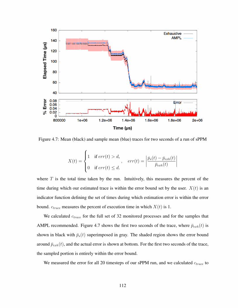
Time (µs)

Ela

pse

d T

ime

(µs)

% E

rro

r

Figure 4.7: Mean (black) and sample mean (blue) traces for two seconds of a run of sPPM

X(t) =

1 if err(t) > d,

0 if err(t) ≤ d., err(t) =

∣∣∣∣ ps(t)− pexh(t)pexh(t)

∣∣∣∣where T is the total time taken by the run. Intuitively, this measures the percent of the

time during which our estimated trace is within the error bound set by the user. X(t) is an

indicator function defining the set of times during which estimation error is within the error

bound. ctrace measures the percent of execution time in which X(t) is 1.

We calculated ctrace for the full set of 32 monitored processes and for the samples that

AMPL recommended. Figure 4.7 shows the first two seconds of the trace, where pexh(t) is

shown in black with ps(t) superimposed in gray. The shaded region shows the error bound

around pexh(t), and the actual error is shown at bottom. For the first two seconds of the trace,

the sampled portion is entirely within the error bound.

We measured the error for all 20 timesteps of our sPPM run, and we calculated ctrace to

112

0.01

0.1

1

10

100

1000

90 / 895 / 5

95 / 398 / 3

99 / 3100 / 0

Ove

rhea

d (ra

tio v

s. u

nins

trum

ente

d)

Confidence / Error bound

Chombo (128 procs, Woodcrest)sPPM (2048 procs, BlueGene/L)

ADCIRC (2048 procs, BlueGene/L)

(a) Percent execution time with TAU tracing

0.01

0.1

1

10

100

1000

90 / 895 / 8

95 / 595 / 3

98 / 3100 / 0

Ove

rhea

d (ra

tio v

s. u

nins

trum

ente

d)

Confidence / Error bound

ParaDiS (8192 procs, BlueGene/P)S3D (8192 procs, BlueGene/P)

Raptor (8192 procs, BlueGene/P)

(b) Percent execution time with effort tracing

100000

1e+06

1e+07

1e+08

1e+09

90 / 895 / 5

95 / 398 / 3

99 / 3100 / 0

Size

of t

race

(in

byte

s)

Confidence / Error bound

Chombo (128 procs, Woodcrest)sPPM (2048 procs, BlueGene/L)

ADCIRC (2048 procs, BlueGene/L)

(c) Output data volume with TAU tracing

100000

1e+06

1e+07

1e+08

1e+09

90 / 895 / 8

95 / 595 / 3

98 / 3100 / 0

Size

of t

race

(in

byte

s)

Confidence / Error bound

ParaDiS (8192 procs, BlueGene/P)S3D (8192 procs, BlueGene/P)

Raptor (8192 procs, BlueGene/P)

(d) Output data volume with effort tracing

Figure 4.8: AMPL trace overhead, varying confidence and error bounds

be 95.499% for our error bound of 8%. This is actually better than the confidence bound we

specified for AMPL. We can attribute this high confidence to AMPL oversampling when it

predicts very small samples (10 or fewer processs), and to sPPM’s general lack of inter-node

variability.

4.4.5 Data Volume and Run-time Overhead

We measured AMPL overhead as a function of sampling parameters. As in §4.4.4, we com-

piled all test applications with AMPL-enabled trace instrumentation. In these experiments

with a fixed number of processors, we varied confidence and error constraints from 90%

confidence and 8% error at the lowest to exhaustive monitoring (100% confidence and 0%

error).

113

For sPPM, Chombo, and ADCIRC, we used TAU with the subset update mechanism. For

ParaDiS, S3D, and Raptor, we used effort instrumentation with the global update mechanism.

In both cases, only those processes in the sample set wrote trace data. Disabled processes did

not write trace data to disk until selected again for tracing by AMPL.

For both sPPM and ADCIRC, we ran with 2048 processes on our BlueGene/L system.

To illustrate that the performance of our library is not tied to a particular architecture, we also

ran Chombo with 128 processes on a smaller Linux cluster. Finally, to test at large scales, we

ran ParaDiS, S3D, and Raptor up to 16,384 processes on a BlueGene/P system.

Instrumentation

The routines instrumented varied from code to code, but we attempted to choose those that

would yield useful metrics for performance tuning. For sPPM, we instrumented the main

time-step loop along with the SPPM routine, and we measured elapsed time for each. Sample

updates were set for every 2 time steps. We ran a total of 20 time steps.

For ADCIRC, we added instrumentation only to the TIME-STEP routine and MPI calls.

ADCIRC sends MPI messages frequently and its time step is much shorter than sPPM, so

we set AMPL’s window to 800 ADCIRC time-steps. We used the mean time taken for calls

to MPI Waitsome() during each window to guide our sampling. MPI Waitsome() is a

good measure of load balance, as a large value indicates that a process is idle and waiting on

others.

For Chombo, we instrumented the coarse time-step loop in the Godunov solver (Colella

et al., 2003a). This time-step loop is of fixed length, although the time-step routine subcycles

smaller time steps as necessary to minimize error. Thus, the number of floating-point instruc-

tions per time-step can vary. We used PAPI (Browne et al., 2000) to measure the number of

floating-point instructions per coarse time-step, and we set AMPL to guide the sample size

using this metric.

114

For ParaDiS, we used effort timings for a call to MPI Waitall in the code’s remesh

phase. As with ADCIRC and �MPI Waitsome, we chose the �MPI Waitall routine to measure

load balance in the code. While we guided using this metric, we recorded data from all effort

regions in our trace.

For S3D, we measured the elapsed time per progress step step for a computation region

in the Z-direction derivative calculation.

Finally, for Raptor, we measured time spent in a computational region in the AMR coarse

time step loop. This loop can adaptively adjust its resolution in both space (by refining a

coarse grid) and time (by sub-cycling time steps).

Time overhead

Figure 4.4.5 shows the measured overhead in time and in data for our experiments. Total

data volume scales linearly with the total processes in the system. In the presence of an I/O

bottleneck, total time scales with the data volume, The experiments illustrate that AMPL is

able to reduce both.

Figures 4.8a shows time overhead for codes instrumented using TAU. The elapsed time

of the sPPM routine varies little between processes in the running application. Hence, over-

head for monitoring SPPM with AMPL is orders of magnitude smaller than the overhead of

monitoring exhaustively. For 90% confidence and 8% error, monitoring a full 2048-node run

of sPPM adds only 5% to the total time of an uninstrumented run. For 99% confidence and

3% error as well as for 95% confidence and 5% error, overheads were 8%. In fact, for each

of these runs, all windows but the first have sample sizes of only 10 out of 2048 processes.

Moreover, AMPL’s initial estimate for sample size is conservative. It chooses the worst-case

sample size for the requested confidence and error, which can exceed the capacity of the

I/O bottleneck on BlueGene/L. If these runs were extended past 20 time windows, all of the

overhead in Figure 4.8 would be amortized over the run.

115

As sampling constraints are varied for ADCIRC, the time overhead results are similar to

the sPPM results. Using AMPL, total time for 90% confidence and 8% error is over an order

of magnitude less than that of exhaustive monitoring.

Time overhead for ADCIRC is higher than for sPPM partly because ADCIRC is more

sensitive to instrumentation. An uninstrumented run with 2048 processes takes only 155

seconds, but the shortest instrumented ADCIRC run took 355 seconds. With sPPM, we

did not see this degree of perturbation. In both cases, we instrumented only key routines,

but ADCIRC makes more frequent MPI calls and is more sensitive to TAU’s MPI wrapper

library. Since sPPM makes less frequent MPI calls, its running time is less perturbed by

instrumentation.

Additionally, the overhead of tracing Chombo is high because the Linux cluster on which

we ran our tests uses a less sophisticated I/O system than that of the Blue Gene/L system.

The Linux cluster uses a single NFS server to handle I/O requests from compute nodes over

the same network used for computation, while the Blue Gene/L system has two dedicated

I/O servers and uses a dedicated network to ship I/O out of the compute partition.

For Chombo, the Woodcrest cluster’s file system was able to handle the smaller load of

128 processor traces well for all of our tests, and we did not see the degree of I/O serial-

ization that was present on our BlueGene/L runs. There was no significant variation in the

run-times of the Chombo runs with AMPL, and even running with exhaustive tracing took

about the same amount of time. However, the overhead of instrumentation in Chombo was

high. In general, instrumented runs took approximately 15 times longer due to the large

number of MPI calls that Chombo makes. This overhead could be reduced if we removed

instrumentation for more frequently invoked MPI calls.

Figure 4.8b shows overhead in percent of total running time for codes instrumented using

our effort scheme. Overhead for ParaDiS and Raptor was similar to that for Chombo. Instru-

mented runs took 9-10x the time of an uninstrumented run because these applications make

116

frequent MPI calls. For Raptor, this is expected, as its code structure is very similar to that of

Chombo. AMPL tracing with 90% confidence and 8% error reduces this overhead by 50%.

For ParaDiS, the input dataset we used for these tests was small, so the effect of PMPI instru-

mentation is very noticeable. For larger, production runs of ParaDiS, this overhead will be

smaller. Nonetheless, using AMPL with 90% confidence and 8% error reduces this overhead

by 13%.

S3D incurs less overhead from tracing because its computation to communication ratio is

much higher. In our tests, an exhaustively instrumented S3D run incurred 37% overhead. An

AMPL-instrumented trace incurred 35% overhead.

Data Reduction

Figures 4.8c and 4.8d show data reduction for different confidence and error settings of

AMPL. For larger runs of SPPM, AMPL can reduce the amount of data that TAU collects by

more than an order of magnitude. With a 90% confidence interval and 8% error tolerance,

AMPL collects only 1.9 GB of performance data for 2048 processes. Sampling all processes

would require over 21 GB of space. Even with a 99% confidence interval and a 3% error

bound, AMPL never collects more than half as much data from sPPM as would exhaustive

tracing techniques.

Data reduction for ADCIRC is even greater. Using AMPL with 90% confidence and 8%

error, data volume for ADCIRC is 28 times smaller than that of an exhaustive trace.

Data overhead for the 128-processor Chombo runs scales similarly to trace volume for

ADCIRC and SPPM. Compared to exhaustive monitoring, we were able to reduce trace data

volume by 15 times compared to an exhaustively traced run with 128 processes. As with both

ADCIRC and sPPM, the sample size and data volume both climb gradually as we tighten the

confidence and error bounds.

For effort-traced codes running on BlueGene/P, we observed similar levels of data reduc-

117

tion. With S3D we saw the most improvement, and traces sampled with 90% confidence

and 8% error were 33 times smaller than exhaustive traces. For Raptor, the same sampling

parameters resulted in a reduction of 12 times, and for ParaDiS we were able to reduce the

data volume by 8 times.

4.4.6 Projected Overhead at Scale

§4.4.5 shows that AMPL’s overhead can be tuned with user-defined sampling parameters, and

it illustrates that AMPL can effectively improve trace overhead on relatively small systems.

However, we would like to know how AMPL’s performance varies as machine size grows.

We configured ADCIRC with TAU and AMPL as in §4.4.5, but in these experiments we

fixed the sampling parameters at 90% confidence and 8% error. Figure 4.9 shows how the

mean sample size, the sample size as a proportion of total system size, and the collected data

volume vary with system size for different codes.

In all cases, the sample size and data volume decrease proportionally with total system

size as the system size increases. This is what we expect. As mentioned in §4.2, sample size

is constant in the limit, so we can expect this curve to level off after 2048 processes, and

we can expect very large systems to require that increasingly smaller subsets of processes be

sampled.

For smaller runs of the TAU-instrumented codes (Figures 4.9a and 4.9b), proportional

sample size and data volume are below 10 percent of the fully-monitored case. On Blue-

Gene/P, sample size for Raptor (Figure 4.9e) and S3D (Figure 4.9d) is less than one percent

of the total for 16,384-process runs. For ParaDiS (Figure 4.9c), a much more variable code,

sample size was less than 5%.

The black line in each of the plots in Figure 4.4.5 shows the absolute sample size as we

increase the process count. For ADCIRC, Chombo, and ParaDiS, the absolute sample size

increases as system size increases. Our runs of ADCIRC and Chombo were on relatively

118

0

10

20

30

40

50

60

70

80

90

100

32 64 128256

5121024

2048 0

10

20

30

40

50

60

70

80

90

100

Perc

enta

ge

Sam

ple

size

(# o

f pro

cess

es)

Total size (# of processes)

Data Volume (% of exhaustive)Sample Size (% of total)

Average Sample Size

(a) Data volume for ADCIRC on BlueGene/L

0

10

20

30

40

50

60

70

80

90

100

8 16 32 64 128 0

10

20

30

Perc

enta

ge

Sam

ple

size

(# o

f pro

cess

es)

Total size (# of processes)

Data Volume (% of exhaustive)Sample Size (% of total)

Average Sample Size

(b) Data volume for Chombo on a Linux cluster

0

20

40

60

80

100

256512

10242048

40968192

16384

0

200

400

600

800

1000

1200

Perc

enta

ge

Sam

ple

size

(# o

f pro

cess

es)

Total size (# of processes)

Data Volume (% of exhaustive)Sample Size (% of total)

Average Sample Size

(c) Data volume for ParaDiS on BlueGene/P

0

10

20

30

256512

10242048

40968192

16384

0

10

20

30

40

50

Perc

enta

ge

Sam

ple

size

(# o

f pro

cess

es)

Total size (# of processes)

Data Volume (% of exhaustive)Sample Size (% of total)

Average Sample Size

(d) Data volume for S3D on BlueGene/P

0

20

40

60

80

100

256512

10242048

40968192

16384

0

200

400

600

800

1000

Perc

enta

ge

Sam

ple

size

(# o

f pro

cess

es)

Total size (# of processes)

Data Volume (% of exhaustive)Sample Size (% of total)

Average Sample Size

(e) Data volume for Raptor on BlueGene/P

Figure 4.9: Absolute and proportional sample size, varying system size

119

0

2e+06

4e+06

6e+06

8e+06

1e+07

0 1 2 3 4 5 6 7 8 9 10

Dat

a vo

lum

e (p

ropo

rtion

of m

axim

um)

Sam

ple

size

(in

proc

esse

s)

Number of clusters

Data Volume (bytes)Avg. Total Sample Size

(a) Data overhead and average total sample size

0

100

200

300

400

500

600

700

800

900

0 1 2 3 4 5 6 7 8 9 10

Tim

e (s

econ

ds)

Number of clusters

ADCIRC

(b) Percent total execution time

Figure 4.10: Data volume in stratified ADCIRC traces

small systems, and their curves appears to increase dramatically at the largest tested sizes.

However, we see with ParaDiS (Figure 4.9c) that this curve begins to level off in the limit,

leading to the gradual reduction in proportional overhead we see in all the plots.

For S3D and Raptor (Figures 4.9d and 4.9e), absolute sample size actually decreases

as system size increases. This implies that the normalized variance of the monitored data is

decreasing as system size increases. S3D is a weak scaling code, so we can expect the number

of behaviors to remain constant as system size increases, which leads to this reduction in

normalized variance over the full system. Raptor is a strong scaling code, but the problem we

tested here is a two-dimensional shock wave. In these experiments, we simulated a relatively

small number of time steps compared to the number that would be simulated in a production

run, so the simulation may not have progressed far enough to yield turbulent flow and other

simulated effects that would trigger adaptation (and thus variability) in Raptor’s solver.

4.4.7 Stratification

We now turn to an examination of AMPL’s performance with stratification. As discussed

in §4.2.3, if we know which groups of processes will behave similarly, we can sample each

group independently and, in theory, reduce data volume. We use simple clustering algorithms

to find groups in our performance data, and we observe that further reductions in data volume

120

are achieved by using these groups to stratify samples taken with AMPL runs.

Clustering algorithms find sets of elements in their input data with minimal dissimilarity.

We used a well known algorithm, k-medoids (Kaufman and Rousseeuw, 2005d), to analyze

summary data from ADCIRC and to subdivide the population of processes into groups.

K-medoids requires a dissimilarity metric to compare the elements being clustered, and

that the user specify k, the number of clusters to find. In our experiment, the elements

were ADCIRC processes. Computing dissimilarity was slightly less straightforward. We

configured ADCIRC as in §4.4.6 and recorded summary data for all 1024 processes in the

run. After each window, processes wrote to a local log file the mean time for all calls to

MPI Waitsome(). The logged data thus consisted of time-varying vectors of local means.

For simplicity, we used the Euclidian distance between these vectors as our similarity mea-

sure.

We ran k-medoids on our 1024-process ADCIRC data for cluster counts from 1 to 10,

and we used the output to construct a stratified AMPL configuration file. We then re-ran

ADCIRC with stratified sampling for each of these configuration files. The single-cluster

case is identical to the non-stratified runs above. Figures 4.10a and 4.10b show data overhead

for different cluster counts and for execution time, respectively.

Figure 4.10a shows that a further 25% reduction in data volume and a 37% reduction in

execution time were achieved on 1024-node runs of ADCIRC by stratifying the population

into two clusters. Surprisingly, for k = 3 and k = 4, dividing the population actually causes

a significant increase both in data volume and in execution time, while 5-10 clusters perform

similarly to the 2-cluster case. Because tracing itself can perturb a running application, there

may be clustering on perturbation noise for the 3 and 4-cluster cases. This inaccurate cluster-

ing is a likely culprit for the increases in overhead, as our samples are chosen randomly and

the balance of perturbation across nodes in the system is nondeterministic. Because we used

off-line clustering, we do not capture this kind of dynamic behavior accurately. This could

121

be improved by using an on-line clustering algorithm and adjusting the strata dynamically.

For the remainder of the tests, our results are consistent with our expectations. With 5-

clusters, the AMPL-enabled run of ADCIRC behaves similarly to the 2-cluster case. Data

and time overhead of subsequent tests with more stratification gradually increase, but they

do not come close to exceeding the overhead of the 2-cluster test. We observe a slow rise

in overhead at 5 or more clusters, and this can be explained by one of the weaknesses of

k-medoids clustering. K-medoids requires that the user specify k in advance, but the user

may have no idea how many equivalence classes actually exist in the data. Thus, the user can

either guess, or he can run k-medoids many times before finding an optimal clustering. If k

exceeds the actual number of groups that exist in the data, the algorithm can begin to cluster

on noise.

4.5 Summary

In this chapter, we introduced a novel tracing technique that uses statistical sampling to re-

duce the volume of trace output to a representative subset of process traces. Our technique

can reduce the data overhead and the execution time of instrumented scientific applications by

over an order of magnitude on small systems. Since the overhead of our sampling scales sub-

linearly with the number of concurrent processes in a system, AMPL shows great promise

for monitoring machines with very large numbers of processes. We also have shown that,

in addition to estimating global aggregate quantities across a large cluster, populations of

processes can be stratified for further reductions in data volume and execution time.

122

Chapter 5

Combined Approach: Adaptive

Stratification

5.1 Introduction

Thus far, we have presented two scalable data-collection techniques. In Chapter 3, we de-

scribed a technique for using low-error, lossy compression to reduce the volume of system-

wide load-balance data across processes and over time in large parallel systems. In Chapter

4, we used adaptive statistical sampling to record only representative portions of a parallel

event trace, and we showed that sampled traces were representative of an exhaustive trace

within certain statistical bounds.

Chapter 4 also showed that sampled tracing could be made more efficient if the trace

were divided, or stratified according to similarity of behavior. We used cluster analysis to

extract equivalence classes from post-mortem exhaustive traces, and we re-ran our adaptive

sampling using clusters as strata. Sample size and trace volume were improved over an

unstratified trace by up to 25%.

Stratification can increase the efficiency of a sample. It also makes complex performance

data understandable. In a large system with data from thousands of processes or more, man-

ually inspecting performance data from each process is tedious. Grouping processes allows

parallel application programmers to understand which processes behave in similar ways by

examining only representative data from each group.

The techniques presented in Chapter 4 rely on post-mortem clustering (or a human) to

stratify the data, which is disadvantageous in two ways. First, the clustering is performed on

uncompressed, un-sampled data, which is not always feasible. For the comparatively small

systems of 2048 or fewer processors that we tested for Chapter 5, clustering exhaustive event

traces is feasible but not practical for on-line monitoring. Our traces consumed gigabytes

of disk storage, and trace clustering was time-consuming, making it unsuitable for on-line

monitoring.

Second, our clustering scheme used a static stratification for the entire application’s exe-

cution. However, as we showed in Chapter 3, the distribution of load in scientific applications

can change dynamically. Ideally, a parallel performance tool would detect when this distri-

bution changes.

In this chapter, we show that combining our system-wide monitoring techniques with

sampling produces a monitoring system that adapts to an application’s behavior at run-

time. We showed in §3.5.1 that our load-balance data-collection framework can gather large

amounts of effort data quickly. Effort traces provide a compressed representation of the be-

havior of all processes in the system, which in turn is passed as input to clustering algorithms

to generate strata.

The bottleneck in this configuration is the cluster analysis. The running time of clustering

algorithms depends on the number of objects to be clustered and on the speed with which we

can evaluate the dissimilarity between these objects. If we cluster on entire process traces

as we did in §4.4.7, then clustering can add significant runtime overhead to parallel tools.

We exploit the multi-scale properties of wavelet data to make this operation fast enough for

on-line use. In particular, we generate a high-level approximation for uncompressed data

124

and then cluster using the approximation. This reduces the volume of data to be clustered

in both the progress and process dimensions of the performance data. We explore the use

of approximations for producing efficient stratification, and we compare our approximate

equivalence classes to those derived through traditional clustering techniques.

The remainder of this chapter is organized as follows. In §5.2 we describe clustering

algorithms and techniques for adapting effort data for clustering. We also detail properties of

wavelet-transformed data that make it particularly efficient for this monitoring scheme. We

describe our equivalence class detection scheme in §5.3. §5.4 details results obtained using

our scheme. Finally, we state our conclusions in §5.5.

5.2 Clustering Effort Data

Recall from §3.4 that our lossy compression scheme aggregates data into two-dimensional,

per-region matrices. Figure 5.1 shows the structure of effort data immediately after aggrega-

tion. For a single region, data from each process is in a row, and progress steps comprise data

from each column. Compression takes place over progress steps (within rows) and across

process identifiers (across rows). The transform across data from different processes is dis-

tributed. A complete data set from one run of our aggregation tool results in a set of these

effort matrices, with one matrix per region of code.

Effort data, immediately after aggregation, is contiguous within regions, but to cluster

it, we must analyze data from separate processes. We cannot change the compression data

layout, because much of the data reduction achieved using wavelet compression results from

inter-process similarity within regions. This section describes how we can reorganize effort

data for effective clustering of inter-process equivalence classes.

125

Effort Data

Pro

ce

ss I

D

Progress

Re

gio

ns

Progress

Single Effort Region System-Wide Effort Dataset

Figure 5.1: Effort data grouped by region, as aggregated by our tool.

5.2.1 Per-process Effort Profiles

An entire effort data set can be thought of as a three-dimensional matrix stored in region-

major order. This arrangement allows quick extraction of profiles of per-region load-balance

properties over time, as shown in §3.6.2. To compare different processes, however, we must

transpose the data set across the progress and region dimensions so that per-process data is

contiguous. The result is a process-major data set as shown in Figure 5.2.

In the transposed data set, each process has a matrix that contains information about the

behavior of all code regions across all time-steps for that process. Each of these matrices

can be considered a signature characterizing the behavior of a particular process, and we can

cluster the signatures to find groups of similarly behaving processes.

This scheme is not inherently scalable. To cluster data like this, we might load the full,

uncompressed effort data into memory, but this can balloon quickly. Effort traces require one

8-byte datum per monitored metric, per monitored code region, per progress step, per pro-

cess. Even if we restricted ourselves to one metric, this is approximately 15 GB for ParaDiS

(8 bytes×16, 384 processes×1024 progress steps×120 effort regions), which would be typ-

ical for short runs. The entire trace will not fit in memory on a single machine, so we cannot

126

Re

gio

ns

Progress

System-Wide Effort Dataset Per-process Effort Signatures

Progress

Re

gio

ns

Figure 5.2: Transposing a data set to make per-process data contiguous.

perform clustering on a single machine. In fact, because our framework operates within in-

strumentation, the memory requirements outstrip what we could use without interfering with

the running application.

5.2.2 Clustering Algorithms

In this section, we describe existing clustering algorithms. We then discuss the specific opti-

mizations that we have developed for sequential clustering on large effort-data sets.

Clustering is a family of techniques for finding groups in data. Typically, the user of a

clustering algorithm has a set of objects (process signatures in our case) to compare using a

particular measure of dissimilarity. Clustering algorithms find groups of objects that mini-

mize this similarity, either optimally or according to some heuristic. While the full taxonomy

of clustering algorithms is beyond the scope of this dissertation, we describe a subset of

relevant algorithms.

K-Means

By far the most commonly used clustering algorithm is the K-Means method (Forgy, 1965;

Hartigan and Wong, 1979; Lloyd, 1982; MacQueen, 1967), which takes a set of objects and

127

a constant k as input. For n objects, K-means groups the points into k clusters so that the

distance of points from the centroid, or mean, of the cluster of which they are a part, is

reduced. While K-means is not optimal, it typically converges very quickly with many fewer

than n iterations. It attempts to minimize squared error and, thus, intra-cluster variance. This

is particularly desirable for our application, because our goal is to reduce the total sample

size, which depends strongly on the variance of observed data.

K-means is disadvantageous because it is not as robust as some other clustering methods.

In particular, it requires algebraic operations to be defined on the clustered objects to enable

the computation of a mean. For some data, this is not defined readily. Further, the represen-

tative of each cluster in a K-means clustering is its centroid, which is likely not identical to

any member of the cluster itself.

In k-means clustering, the user must pick k, the number of clusters, in advance. This can

be disadvantageous because often k is not known, and it depends on the specific structure of

the data. This is somewhat paradoxical, as one generally hopes to determine this structure

by using clustering. For data sets where the number of clusters is small, this deficiency can

be overcome by running multiple trials of K-means and varying k. The resulting clusters

may be evaluated using a clustering criterion (Meila, 2005; Sherwood et al., 2003) to assess

their quality. Generally clustering criteria assess how well dissimilarity is minimized within

clusters. The result of the trial with the best clustering criterion is then selected as the result.

WaveCluster

Another clustering algorithm, WaveCluster (Sheikholeslami et al., 2000), uses a wavelet

transform to perform clustering on graphical data at multiple scale levels. The algorithm

examines wavelet coefficients at different scale levels, then groups points based on their prox-

imity at different scales. Like our compression scheme, WaveCluster uses a two-dimensional

wavelet transform on its data. It may seem that we could apply this technique directly to our

128

performance data, but our data is more complex than the graphical data for which WaveClus-

ter was designed. While WaveCluster clusters individual points, our algorithm clusters entire

effort signature matrices from multiple processes. Our distance metric is more complicated,

and to apply WaveCluster to our data, we would need to generalize its approach for very

high-dimensional wavelet transforms.

Subspace Clustering

Subspace clustering (Parsons et al., 2004) is a technique for finding similar groups in very

high-dimensional data. Unlike other clustering algorithms, subspace clustering algorithms

do not use a single distance metric. Rather, subspace clustering attempts to find objects in a

dataset that are correlated in some subspace of the full set of dimensions in the data. However,

subspace clustering does not require clusters to be self-similar in the same set of dimensions.

Subspace clustering techniques are helpful for understanding higher-dimensional data

because they can select both similar sets of objects and the dimensions in which the objects

are similar. To accomplish this, they typically use some form of dimensionality reduction

to discover which dimensions are correlated within the data set. Such algorithms could be

applied to high dimensional performance data to correlate application-level measures such as

progress and effort with hardware performance counter data.

Hierarchical Clustering

Hierarchical or agglomerative clustering (Murtagh, 1985) is a recursive technique that starts

with a set of objects and combines the closest objects into a single cluster during each step.

The resulting clustering is not a set of distinct groups, but a hierarchy of increasingly large

groups. At the root of the tree is the full dataset, and its leaves are individual objects. This

tree is commonly called a dendrogram, and it can be partitioned into groups to form flat

clusterings like those produced by K-means.

129

Depending on the algorithm, hierarchical clustering requires O(n2) or O(n2log(n)) time

to run, and the bulk of the running time is consumed by the computation of a dissimilarity

matrix, which holds the pre-computed dissimilarities of all pairs of objects in the data set. We

could easily apply this algorithm to our data, and we could use the multi-level structure of

the clusters that it generates to ease navigation of output data from clusterings, or to modify

sampling stratifications at runtime.

In §5.4.1, we apply hierarchical clustering to effort data to demonstrate the feasibility of

this approach with our approximation matrices. However, to use hierarchical clustering ef-

fectively, we would need to determine how best to ”cut” the dendrogram into a flat clustering

of per-process data. We would also need to determine a suitable type of linkage between

clusters, where linkage refers to the way in which an algorithm computes the distance be-

tween two clusters as a function of the distances of their members. In this dissertation, we

are concerned primarily with methods for sampling cluster data, so we have elected to use a

simpler clustering algorithm for on-line clustering.

K-Medoids

K-medoids is a family of clustering algorithms very similar to K-Means, but these methods

do not require that algebraic operations be defined on the data. K-medoids is useful in cases

where only the dissimilarities between objects can be computed. Like K-means, it takes the

number of clusters k as input and attempts to minimize squared error between k subsets of the

original data. However, instead of partitioning based on proximity to centroids, K-Medoids

partitions relative to representative elements from each cluster called medoids.

We have chosen to use K-Medoids in our experiments for three reasons. First, K-Medoids

directly attempts to minimize squared error among elements in the clustering. This is directly

analogous to reducing variance in the input data set, which will roughly correspond to the

variance within clusters. It will thus produce a stratification that improves sample size.

130

Second, K-Medoids facilitates analysis by providing a representative from each cluster,

which is useful to analysts for a usability standpoint. With K-Means, selecting points closest

to the centroids can produce cluster representatives, without the same optimality guarantees

that K-Medoids provides.

Finally, K-Medoids only requires that we formulate a distance measure between input el-

ements (effort regions), and we already have a basic notion of dissimilarity between matrices

in the Root Mean Squared Error measure described in §3.6.1.

The most basic implementation of K-Medoids, PAM (Kaufman and Rousseeuw, 2005c),

requires O(n2) time to run. As for hierarchical clustering, the bulk of this running time is

consumed by the computation of a dissimilarity matrix. For our problem, n is the process

count, and objects are per-process effort signatures.

For large n, this algorithm can be costly, but there is a sampled variant of K-Medoids,

CLARA (Kaufman and Rousseeuw, 2005b). Instead of clustering an entire data set, CLARA

runs PAM on subsets of the full data set and assigns each object to the nearest medoid from

the PAM run. Typically this process is repeated several times. The best clustering is cho-

sen from the results based on the sum of dissimilarities of objects to their closest medoid.

CLARA runs in O(n+s2S) time, where s is the size of the sample and S is the number of it-

erations. If s is chosen to be less than or equal to√n, then the time and storage requirements

of CLARA are linear in the size of the dataset rather than quadratic.

Like K-Means, K-Medoids requires that the user specify k in advance, and this may

be overcome for small k by conducting a number of clustering trials and selecting the best

candidate according to a clustering criterion.

5.2.3 Parallel Clustering Techniques

Clustering techniques are used heavily for statistical analysis, data mining, and other data-

intensive applications. Many parallel clustering implementations have been attempted. We

131

summarize them below.

Parallel K-Means Clustering

A number of distributed-memory parallel K-Means algorithms have been developed. Ranka

and Sahni (Ranka and Sahni, 1991) describe an algorithm for K-Means clustering for use in

image-analysis applications. Their algorithm runs on supercomputers with hypercube inter-

connect topologies. The authors showed that this algorithm scales to 64 cores with roughly

50% parallel efficiency when clustering 16,384 data points. Stoffel and Belkoniene (Stoffel

and Belkoniene, 1999) present another parallel K-Means implementation that achieves 90%

parallel efficiency on as many as 32 processors for data sets of 100,000 objects. Forman and

Zhang (Forman and Zhang, 2000b; Forman and Zhang, 2000a) present a similar K-Means al-

gorithm that achieves nearly linear speedup for as many as 128 processors with object counts

up to 10 million nodes. Finally, Kraj et al. present ParaKMeans, a publicly available parallel

K-Means algorithm for K-Means clustering that can be used through a web interface. Their

algorithm achieves 5x speedup with 7 processors and 10,000 data points. Depending on k,

the speedup of ParKMeans levels off between 4 and 7 processes, and there is no marginal

speedup after this point.

Parallel Hierarchical Clustering

Parallel Hierarchical clustering has been studied extensively. Olson (Olson, 1993) presents

optimal hierarchical clustering algorithms. In addition to shared-memory algorithms, he

presents an algorithm for butterfly networks of n processors that runs in O(nlog(n)) time.

Rajasekaran (Rajasekaran, 2005) improves on this work by defining tighter bounds for the

expected running time. His algorithm runs in O(log(n)) time on a system with n processors

in the average case, but it assume that the data points to be clustered are distributed uniformly

among processors, which does not always hold in practice.

132

Du and Lin (Du and Lin, 2005) present a hierarchical clustering implementation for ma-

chines running MPI. They perform experiments with three biological gene-expression data

sets representing 7,452, 9,217, and 11017 genes, respectively. For the smallest data set, they

achieve 25x speedup with 48 processors. For the larger data sets, speedup is around a factor

of 15 with the same number of processors. The authors report that this speedup increases

linearly with system size, and marginal speedup does not decrease before 48 processors.

Wang et al. (Wang et al., 2008) present another hierarchical clustering implementation

using MPI, but they conduct experiments on financial data. They show an 8x speedup using

16 processors and a 9x speedup using 32 processors, but marginal speedup diminishes after

this point.

Parallel Subspace Clustering

Nagesh et al. have implemented a parallel subspace clustering algorithm, pMAFIA, in MPI.

pMAFIA partitions the space to be clustered evenly among processors. The authors conduct

experiments on an IBM SP2 cluster with 16 processors. With a large data set containing

8.3 million records, the communication required for pMAFIA is negligible compared to the

amount of computation. The authors report near-linear speedup when clustering this data on

as many as 16 processors.

Parallel K-Medoids Clustering

Kaufman and Hopke (Kaufman et al., 1988; Hopke, 1990) developed and ran a parallel

version of the CLARA K-Medoids clustering algorithm described in §5.2.2. Rather than par-

allelize the full algorithm, they presented two approaches that take advantage of the sampled

nature of CLARA. Since CLARA executes multiple sampled trials of PAM, their approach

distributes the sampled trials across a cluster of 10 processors. Good performance was re-

ported, but specific numbers were not provided.

133

Using Parallel Clustering with Effort Data

A natural solution to the data-volume problem would be to investigate parallel clustering

algorithms for effort data. As discussed above, there is much existing work on parallel clus-

tering, some of which has achieved linear speedup. However, the focus of most existing work

has been on partitioning very large data sets among a small number of processors. Effort data,

on the other hand, is nearly completely distributed, and we would need to design a clustering

algorithm with much more communication and with smaller amounts of data per processor

than those described here.

Clustering algorithms for entirely distributed data have been developed. Bandyopadhyay

and Coyle (Bandyopadhyay and Coyle, 2003) present a distributed hierarchical clustering

algorithm aimed at reducing power consumption in distributed sensor networks. Their al-

gorithm groups sensors into a single-level hierarchy in which each sensor sends data to a

clusterhead1. When all sensors report to their clusterheads instead of directly to a centralized

data sink, energy consumption in the sensor network is minimized.

The problem of conducting a full parallel clustering of effort data is more similar to the

problem of clustering data on sensor networks than to traditional data-intensive clustering

approaches. However, existing work in sensor networks has focused on energy reduction,

while we are interested in conducting intensive analysis within our network of processors.

Adapting existing algorithms for this purpose is a difficult problem that lies beyond the scope

of this dissertation. In this work, we have investigated clustering strategies for single-node

machines using effort approximations to reduce the volume of data to be clustered.

5.2.4 Using Wavelets for Approximation

Both PAM and CLARA require that we store the entire data set in memory on the node

running the clustering algorithm. PAM requiresO(n2) space, and CLARA requiresO(n+s2)

1A clusterhead in this context is roughly analogous to a cluster centroid.

134

. . .

. . . . . .

si di

di si di di

si di

di si di di

11

11

11

22

22

22

si siLL

(a) Level L transform

si di

di si di di

si di

di si di di

11

11

11

22

22

22

di si33

si di33

di di33

si si33

(b) Level 3 approximation

si di

di si di di

si di

di si di di

11

11

11

22

22

22

si si22

(c) Level 2 approximation

si di

di si di di11

11

11

si si11

(d) Level 1 approximation

si si00

(e) Full reconstruction

Figure 5.3: Structure of coefficients after applications of the inverse wavelet transform

space. Neither approach is scalable, because n for our problem would be the number of

processes in the full parallel system.

The wavelet representation provides an effective solution to this problem. Recall from

§3.3 that we can analyze wavelet-compressed data at hierarchical scales and levels of detail.

We can use this property of the wavelet transform to generate a coarse-grained approximation

of our per-process effort signatures. Thus, we can cluster on a much smaller representation

of the same data instead of on the uncompressed data set.

Figure 5.3a shows the organization of two-dimensional wavelet coefficients for a level-L

transform. sli and dli represent low-frequency and high-frequency coefficients, respectively,

for the level-l application of the wavelet transform. Coefficients at level 1 represent informa-

tion from the input data with the highest frequency and finest granularity, and coefficients at

successively deeper levels represent coarser-grained information. Level-L coefficients repre-

135

sent the coarsest features. Each level l contains one-fourth as many coefficients as level l−1,

so the bulk of the space is consumed by high-frequency coefficients.

The low-frequency coefficients sli at deeper levels of the wavelet transform are a smaller,

coarser-grained approximation of the input data, and the high-frequency coefficients dli repre-

sent the details that were removed to create these approximations. Decompressing an effort

file requires that we first EZW-decode the transformed data, then add each level of detail

back into the image by applying successive inverse wavelet transforms. Typically, the in-

verse transform is applied L times to reconstruct the input data s0i . This process is shown in

Figure 5.3.

We can also create a level L − i approximation of the input data by applying only i

inverse transforms. Figures 5.3b, 5.3c, 5.3d, and 5.3e show the structure of coefficients after

inverse transforms are applied to obtain levels 3, 2, 1, and 0, respectively. The coefficients

that comprise the approximations are highlighted in bold.

We can now EZW-decode compressed effort data and construct an approximation at an

arbitrary level, but one complication remains. The EZW encoding algorithm, which con-

tributes greatly to the effectiveness of our compression algorithm, operates on the full data

for each compressed region. Each EZW pass measures the significance of all wavelet coeffi-

cients against a particular threshold. Thus, each pass requires a full traversal of the wavelet

coefficients.

The original EZW algorithm (Shapiro, 1993), used a Morton scan (Morton, 1966) for this

purpose, while the parallelized version uses a depth-first traversal of the coefficients (Ang

et al., 1999). In both cases, data from the same level in the transformed coefficients is non-

contiguous. Because the EZW encoding is embedded, we cannot simply jump to the level

of interest in an EZW stream. With an unmodified EZW algorithm, we would be forced

to create a matrix large enough to hold all compressed wavelet coefficients for each effort

region that we explore.

136

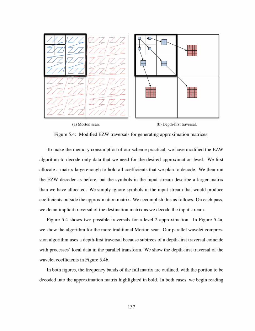
(a) Morton scan. (b) Depth-first traversal.

Figure 5.4: Modified EZW traversals for generating approximation matrices.

To make the memory consumption of our scheme practical, we have modified the EZW

algorithm to decode only data that we need for the desired approximation level. We first

allocate a matrix large enough to hold all coefficients that we plan to decode. We then run

the EZW decoder as before, but the symbols in the input stream describe a larger matrix

than we have allocated. We simply ignore symbols in the input stream that would produce

coefficients outside the approximation matrix. We accomplish this as follows. On each pass,

we do an implicit traversal of the destination matrix as we decode the input stream.

Figure 5.4 shows two possible traversals for a level-2 approximation. In Figure 5.4a,

we show the algorithm for the more traditional Morton scan. Our parallel wavelet compres-

sion algorithm uses a depth-first traversal because subtrees of a depth-first traversal coincide

with processes’ local data in the parallel transform. We show the depth-first traversal of the

wavelet coefficients in Figure 5.4b.

In both figures, the frequency bands of the full matrix are outlined, with the portion to be

decoded into the approximation matrix highlighted in bold. In both cases, we begin reading

137

the EZW stream and we only do the update if it falls within the bounds of the approximation

matrix when we need to write a coefficient to the matrix. Because the EZW encoding is

embedded, we must still do a full traversal and read all symbols on the input stream. In the

figure, parts of the traversal that write coefficients are shown in blue, while parts that only

read from the input stream are shown in red.

Although we show full traversals in the figure, the EZW algorithm encodes a special

zerotree coefficient that allows us to skip insignificant subtrees on each pass. Thus, while

the exhausted data is O(n) in the number of processes in the monitored system, the decod-

ing process is bounded by the size of the compressed data. We showed in §3.5.2 that we

achieve from 100:1 to 1000:1 compression ratios; thus decoding on a single node remains

manageable, even on large systems.

5.2.5 Measuring Dissimilarity

Because we can generate approximation matrices efficiently, we can define an efficient dis-

similarity measure for per-process effort signatures. We can use this measure to construct an

efficient clustering algorithm.

In §4.4.7, we did simple K-Medoids clustering on entire event traces using the Euclidean

distance between trace vectors as our dissimilarity measure. Here, because we are comparing

processes by multiple regions of code instead of by a single metric, we use a slightly more

complicated distance measure.

Given an effort data set with r regions, n processes, and p progress steps, we can transpose

the data set to produce a set of n per-process effort signature matrices, each with dimensions

r × p. We define the dissimilarity of two effort signatures, E = {eij} and F = {fij}, as the

138

Euclidean distance between vectors of row means:

Dall(E,F ) =

√√√√ r∑i=0

[∑pj=0 eij

p−∑p

j=0 fij

p

]2

(5.1)

We use the mean over progress steps because we will use this approximation in an on-line

setting. Because we will recompute the clustering periodically as an application runs, we

do not account directly for variation over time. Instead, our on-line algorithm clusters sub-

sequent time windows separately, as AMPL does, which allows the algorithm to adapt to

variation over time.

K-Medoids requires that we apply Dall O(n2) times, and each application requires O(rp)

work. We can assume that the number of regions is small (100-200), and if we do clustering

on-line instead of post-mortem, we can assume also that the number of progress steps is much

smaller than the full number of progress steps in a run. If we cluster on approximate data,

then we can reduce n and p significantly.

When applied to level-l approximations of E and F , El = {elij} and F l = {f lij}, Dall

becomes:

Dapprox(El, F l) =

√√√√ r∑i=0

[∑p′

j=0 elij

p′−∑p′

j=0 flij

p′

]2

, p′ =p

4l(5.2)

Likewise, the complexity of Dapprox is reduced to O(rp/4l), and the complexity of K-

Medoids clustering using Dapprox is now O(n2/16l).

5.2.6 Neighborhoods of Points

Clustering on approximations of the original data is not perfect, as the approximations are

lossy. When we compare approximations of effort signatures, each coefficient represents

the values of a neighborhood of coefficients in the full data. Figure 5.4b shows parent-

139

child relationships of coefficients in the wavelet quad-tree. Each coefficient represents a

neighborhood in the original data corresponding to its descendants at level 0 of this tree. For

higher-level approximations, each point in the approximation represents more points in the

original image. Thus, using smaller approximate representations increases the risk of losing

important data about our processes.

The accuracy of our approximations depends strongly on the degree of locality in the full

effort-measurement space. An easily approximated effort region will have strong locality in

both the progress and process dimensions, because these are the dimensions that our com-

pression algorithm reduces in size. Ideally, the local topology of our compression scheme, a

hierarchical quad-tree spanning processes and time, will map well to the application’s own

communication topology in these dimensions.

The progress dimension exploits temporal effort consistency in the application, if it exists.

Progress increases monotonically with application execution, and it would not make sense,

especially in an on-line algorithm, to reorder the progress dimension. However, one short-

coming of our current compression scheme is that the second dimension is process identity.

Process identity is easy to obtain, as every process in an MPI application can know its rank;

however, it does not necessarily map to the simulation topology in an application. Unmatched

topologies could be disadvantageous if an application’s behavior has strong locality within

its simulation space. Many applications use more sophisticated communication topologies,

and mapping our compression scheme to these would require significant changes.

For example, a simulation might use a three-dimensional communication topology pro-

jected onto the one-dimensional process-identity space. Neighbors in this space are not nec-

essarily neighbors in the process-identity space. Further, representing a neighborhood of

points with a single value might incur more error than if the simulation assumed that nodes

were laid out in a straight line. Taking this into account in our compression scheme leaves

us with two choices. We could increase the dimensionality of our wavelet transform such

140

Sampled

Monitoring . . .

Decompress Approximate Effort Dataset Transposed Effort Dataset K-Medoids

Effort Clustering Algorithm

Com

pre

ssio

n

Re-s

tratify

Effort

Clustering

Com

pre

ssio

n

Re-s

tratify

Effort

Clustering

Com

pre

ssio

n

Re-s

tratify

Effort

Clustering

Progress . . . 3 4 5 6

Sampled

Monitoring

7 8 9 . . .

Pro

cesses

Figure 5.5: On-line stratification framework.

that the application’s dimensions and the progress dimension correspond one-to-one with the

dimensions of the transform. Alternately, we could attempt to reorder the process identifiers

used in our compression scheme to correspond to some locality-optimizing, space-filling

curve embedded in the application’s topology.

Engineering either of these approaches and testing the associated performance perfor-

mance impact is beyond the scope of this dissertation, but we mention these possibilities

here for completeness. Currently, our approach only uses MPI rank order for the process-

identity dimension, but our results show that this preserves enough behavioral locality to be

beneficial.

5.3 On-line Stratified Sampling

We have applied the techniques discussed in §5.2 to devise a framework for adaptively strati-

fying a running parallel system into equivalence classes at runtime. We leverage system-wide

141

data obtained through our lossy compression scheme to reduce the overhead of sampled trac-

ing through clustering, and we leverage the hierarchical nature of wavelet data to accomplish

this within a reasonable amount of time.

Figure 5.5 shows how components in our framework operate over time. As with AMPL,

we sample the population on successive progress steps and we define an update interval, a

number of steps after which we adapt our sampling scheme. The figure shows our scheme

with an update interval of three progress steps.

The squares at the top of the figure represent processes in a parallel application. After

the first update interval, we use our compression scheme to aggregate system-wide effort

data onto a single node. We then apply our clustering algorithm (shown in the gray inset).

We partially decompress the data to produce an approximate data set. We then transpose the

approximation along the process identity and region dimensions, and we perform K-Medoids

clustering on the per-process effort signatures. Next, we use these clusters to update the

stratification.

To convert a clustering on our approximate data set to a stratification of the full system,

we replace each process identifier in the clustering with the corresponding neighborhood of

process identifiers in the full system. That is, for a level-l approximation, process identifier i

in the approximation corresponds to IDs j in the full data set, where j ∈[2li . . . 2li+ 2l − 1

].

Once we have computed a new stratification, we can broadcast this data efficiently to the

remote processes, recompute the minimum sample size for each stratum, and monitor each

stratum separately until the next update. We compute the intra-stratum variances slightly

differently than in §4.3. Instead of computing the variance from the approximate represen-

tation, in which where there may be extra noise due to compression, and using this as an

estimator of the stratum variance, we use an efficient reduction operation available on most

high-performance machines to compute the actual variance for the entire system. This does

not add significant overhead to our scheme, because we already run a similar operation, but

142

with much more data, in our wavelet-compression scheme. Thus, we use the actual variance

from the current interval to guide the sample size for the next.

5.4 Results

To assess the effectiveness of our clustering and sampling schemes for on-line use, we con-

ducted extensive tests using system-wide data collected from scientific applications. Because

our stratification and sampling schemes operate within a single process, we conducted our

experiments off-line, but we used post-mortem application data from two scientific appli-

cations as input to our algorithms. We were thus able to measure the performance of our

algorithms and verify their results against uncompressed data.

For the tests conducted here, we used output from the ParaDiS (Bulatov et al., 2004) dis-

location dynamics simulation and the S3D (Hawkes and Chen, 2004) turbulent-combustion

code. Both of these codes are described in detail in §3.5.

The rest of this section is organized as follows. In §5.4.1, we demonstrate the speedup

obtained by clustering with approximations on effort data sets. We then show that clusterings

obtained using approximations are nearly identical to those obtained using exhaustive data. In

§5.4.2, we show that our results from §5.4.1 extend to transposed data sets of effort signatures.

Finally, in §5.4.3, we illustrate the benefits of our stratified sampling scheme for data from

real application runs.

5.4.1 Clustering Speed

To test the scalability of our clustering algorithm and to gauge the speedup and error achiev-

able using approximation matrices in place of exhaustive data, we first conducted test runs of

a hierarchical clustering algorithm on untransposed effort-data sets. We clustered across re-

gions, grouping those with similarly shaped load distributions. This analysis could be used to

143

0.1

1

10

100

1000

10000

8 16 32 64 128 256 512

Clu

ster

ing

Tim

e (s

econ

ds)

Approximation Matrix Size

20 regions40 regions

132 regions*

(a) Time required to cluster approximations.

0 0.03 0.06 0.09 0.12 0.15 0.18 0.21 0.24 0.27 0.3

8 16 32 64 128 256 512

Nor

mal

ized

Mirk

in D

ista

nce

Approximation Matrix Size

20 regions40 regions

132 regions*

(b) Error compared to exhaustive data.

Figure 5.6: Time and error in clustering effort regions with approximations.

trace load imbalances with similar root causes to specific effort regions. For our dissimilarity

metric, we used the root mean-squared error between regions. In contrast to our methods

in §3.6.1, we did not normalize the RMS error, because we are interested in using this as a

dissimilarity measure and not as a means of checking percent error.

For our test sample data set, we used a 512-process, 512 progress step trace of ParaDiS,

which we showed in §3.6.2 to have regions with very different load distributions. For the

hierarchical clustering software, we used Google’s scipy-cluster package (Eads, 2008) along

with custom Python wrappers for our effort objects implemented in C++. We ran these

tests on a modest 2.40 GHz Pentium 4 Xeon system with 512 megabytes of Random Access

Memory (RAM).

Figure 5.6a shows the time in seconds required to run hierarchical clustering while vary-

ing approximation size and number of effort regions. In total, our ParaDiS data set contained

data for 132 effort regions. Clustering the complete data set at full size required over two

hours to run, which is clearly unacceptable for use in an on-line setting. However, the time

required to cluster decreased significantly for higher approximation levels and as we reduced

the number of regions clustered. For 20 regions and an 8× 8, level-6 approximation, cluster-

ing took less than a second. In both 20 and 40 regions, clustering took less than 10 seconds

for approximation levels of 3 or greater (64 × 64 or smaller matrices). The approximate

144

clustering thus can run over 1000 times faster than the exhaustive clustering.

To gauge how well our clustering scheme approximates clustering with full data, we

arbitrarily flattened the dendrograms generated by our hierarchical clustering scheme into 10

clusters. We then used the Mirkin distance (Mirkin, 1996; Meila, 2005) as a metric.

Let a clustering C be defined as a set of N clusters Ck for k = 0 . . . N − 1. Each cluster

Ck contains nk objects, such that |Ck| = nk, and∑N−1

k=0 nk = n. Given two clusters, Ck and

C ′k, let the number of points in their intersection be:

nkk′ = |Ck ∩ Ck′ | (5.3)

Further, given two clusterings on the same data set, C and C ′, the Mirkin distance between

them is defined as:

d’M(C,C ′) =N−1∑k=0

n2k +

N−1∑k′=0

n′2k′ − 2N−1∑k=0

N−1∑k′=0

n2kk′ (5.4)

Put simply, the Mirkin distance measures the number of pairs of points that are in the same

cluster in C but in different clusters in C ′. It is used throughout the literature to assess the

quality of clustering algorithms such as ours. For our comparisons, we use the normalized

Mirkin distance, which is invariant to the size of the data set. It is defined as:

dM(C,C ′) =d′M(C,C ′)

n2(5.5)

Figure 5.6b shows the normalized Mirkin distance between clustering using approxima-

tions and clustering using exhaustive data for the same set of experiments as is shown in

Figure 5.6a. We see that even for an 8 × 8, level-6 approximation, the clustering error is no

higher than 21%. For level-5 and lower approximations, the error of clustering is between

10% and 15% in clustering 20 regions, but much less in clustering 40 regions (no error) or

145

132 regions (only 6%). Surprisingly, there is a spike in clustering all regions for the level-2,

128 × 128 approximation, which indicates that we can actually do better with coarser, level

3-5 approximations than with larger, more costly ones. We hypothesize that this anomaly

arises from noise in the data that is present at level 2, but that is filtered at higher levels of

approximation. At the very least, our data shows that clustering with approximate effort data

can yield considerable speedup with a nominal cost in clustering accuracy.

5.4.2 Clustering Transposed Data Sets

We showed in the previous section that a level-l wavelet approximation can speed up clus-

tering of effort regions by reducing the size of the input data set by 4l. In this section, we

exploit this property to reduce the speed and memory requirement of clustering algorithms

for system-wide data from large clusters.

We generated data for this section with runs of S3D on as many as 16,384 processes on

Argonne National Laboratory’s Blue Gene/P supercomputer. For each run, we ran S3D for

200 time steps, recorded full effort data, and stored it to disk. For our tests, we loaded this

data back into memory, and we ran our framework using windows of progress data from this

stored data as input rather than windows of progress from data collected at runtime. Because

the data is the same for each trial, this approach provides reproducibility that could not be

achieved with repeated runs.

Clustering Exhaustive Effort Data

Clustering across processes is expensive because the number of processes grows with the

size of the parallel system. Because most clustering algorithms are O(n2), the time required

to cluster data from large numbers of processes, particularly from thousands or more pro-

cesses, becomes impractical for on-line use. Figure 5.7a shows the time required to cluster

10 progress steps using both the PAM and CLARA K-Medoids methods on exhaustive data

146

0.1

1

10

100

1000

10000

512 1024 2048 4096 8192 16384

Clu

ster

ing

Tim

e (s

econ

ds)

Size of data set (processes)

PAMDecompression

CLARA

(a) Time for clustering operations, varying systemsize

0 0.05 0.1

0.15 0.2

0.25 0.3

0.35 0.4

512 1024 2048 4096 8192

Nor

mal

ized

Erro

r

Size of data set (processes)

Mirkin distance% Difference in avg dissimilarity

(b) Normalized error of CLARA vs. PAM

Figure 5.7: Using CLARA and PAM on effort data

sets for various system sizes. The figure also shows the time required to decompress the

effort-data set fully.

For PAM, clustering is only fast enough to consider using on-line for the 512-process

data set, which takes around 6 seconds. For 1024 nodes, clustering requires 25 seconds, and

increases quadratically with system size from here. For an 8192-process data set, clustering

10 progress steps takes 35 minutes, and for 16,384 processes, the system exceeded available

memory and began to thrash.

CLARA runs much faster than PAM, taking less than 10 seconds for all data sets, over

two orders of magnitude faster. In the slowest case, for 16,384 cores, CLARA took just

under 7 seconds to cluster 16,384 processes. This is suitable for on-line use. To ensure

that CLARA’s clusterings were close to the near-optimal clusterings computed by PAM, we

compared CLARA’s output to PAM’s with two error metrics. First, we used the normalized

Mirkin distance, as discussed in §5.4.1. We also compared the difference in average dissim-

ilarity between objects and their nearest medoids. This is the measure used within CLARA

to evaluate the quality of sub-calls to PAM.

Figure 5.7b shows our results. We cannot show results for 16,384 processes since we

could not run PAM at this scale. For 512-, 4096-, and 8192-process runs CLARA and PAM

147

produced the same clusterings, and the normalized Mirkin distance is zero. However, the

average dissimilarity for CLARA’s clusterings is 3-4% higher than that for PAM’s output.

This indicates that the medoids found by CLARA are slightly further from the center of

their clusters than those found by PAM, which is to be expected from a sampled-clustering

algorithm. For 1024- and 2048-process runs, the normalized Mirkin distance does not exceed

10 percent, so the clusterings found by CLARA are very close to those found by PAM. The

average dissimilarity is again higher for CLARA, this time by around 25%, indicating that

again CLARA’s medoids are not chosen as well as PAM’s.

CLARA is notably more scalable than PAM, and slightly less accurate medoids are a

small price to pay for the huge speed gains that we see with CLARA. However, CLARA

does not solve the memory problems or avoid the need to decompress the full effort-data

set. Figure 5.7a shows that decompression takes about an order of magnitude less time than

running PAM for the larger cluster sizes, but it still requires close to five minutes at 16,384

nodes. This is not suitable for on-line usage. Further, even if we can decompress the full

data set, there is a significant cost in memory. The full, 200 progress-step trace of S3D

consumes 3.2GB when fully expanded, and 10 steps of it consume 160MB, which is still too

large to run inside instrumentation without perturbing or crowding the monitored application

significantly.

Improving Clustering Time Using Approximations

We showed in §5.4.1 that using wavelet approximations can greatly increase the speed of

clustering regions. Similarly, we can use approximate transposed data sets to reduce the

clustering time for behavioral equivalence class detection among processes.

Figure 5.8a shows the time required to decompress approximate effort data sets. With

only two levels of approximation, we can reduce the decompression time for even 16,384-

process data sets to ten seconds or less. Figure 5.8b shows the time required to run CLARA

148

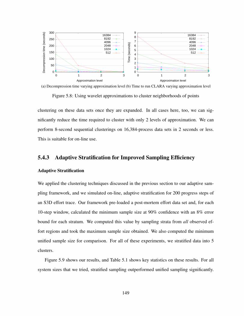
0

50

100

150

200

250

300

0 1 2 3

Dec

ompr

essi

on ti

me

(sec

onds

)

Approximation level

163848192409620481024

512

(a) Decompression time varying approximation level

0 1 2 3 4 5 6 7 8 9

0 1 2 3

Tim

e (s

econ

ds)

Approximation level

163848192409620481024512

(b) Time to run CLARA varying approximation level

Figure 5.8: Using wavelet approximations to cluster neighborhoods of points

clustering on these data sets once they are expanded. In all cases here, too, we can sig-

nificantly reduce the time required to cluster with only 2 levels of approximation. We can

perform 8-second sequential clusterings on 16,384-process data sets in 2 seconds or less.

This is suitable for on-line use.

5.4.3 Adaptive Stratification for Improved Sampling Efficiency

Adaptive Stratification

We applied the clustering techniques discussed in the previous section to our adaptive sam-

pling framework, and we simulated on-line, adaptive stratification for 200 progress steps of

an S3D effort trace. Our framework pre-loaded a post-mortem effort data set and, for each

10-step window, calculated the minimum sample size at 90% confidence with an 8% error

bound for each stratum. We computed this value by sampling strata from all observed ef-

fort regions and took the maximum sample size obtained. We also computed the minimum

unified sample size for comparison. For all of these experiments, we stratified data into 5

clusters.

Figure 5.9 shows our results, and Table 5.1 shows key statistics on these results. For all

system sizes that we tried, stratified sampling outperformed unified sampling significantly.

149

Procs Avg. unified Avg. stratified Net improvement # Improved % Improved1024 514 201 61% 145/200 72.4%2048 825 317 62% 145/200 72.4%4096 1213 450 63% 139/200 69.5%8192 1722 663 61% 132/200 66.0%16384 2331 1026 56% 121/200 60.5%

Table 5.1: Improvements in sample size using adaptive stratification with S3D.

Procs Avg. unified Avg. stratified Net improvement # Improved % Improved1024 514 590 -14.7% 41/200 20.5%2048 825 1023 -23.9% 39/200 19.5%4096 1213 1705 -40.6% 36/200 18%8192 1723 2769 -60.7% 37/200 18.5%16384 2331 4378 -87.8 % 33/200 16.5%

Table 5.2: Decrease in sampling efficiency using approximate clustering on S3D data.

The unified sample size is shown in red, while the total stratified sample size (the sum of

sample sizes from each cluster) is shown in blue. Depending on system size, we reduced

the total sample size by an amount between 60% and 70%. On average, we saw a 60%

improvement in sampling cost over the entire run when using adaptive stratification. With

the number of clusters held constant, the improvement from stratification decreases as system

size increases, but only slightly. The limits on this improvement may arise from monitoring

a decreasing percentage of the full system in the first place.

Adaptive Stratification with Approximate Clustering

We repeated the previous experiment, using approximate effort data to guide the clustering

instead of clustering a full data set. In these experiments, we clustered on a transposed,

level-1 effort approximation, and we then expanded the approximate process identifiers by

replacing them with their corresponding neighborhood of process identifiers in the full data

set. Figure 5.10 shows the results; Table 5.2 shows key statistics analogous to those presented

for adaptive stratification with full data.

150

0

200

400

600

800

1000

1200

0 20 40 60 80 100 120 140 160 180 200

Sam

ple

size

(# p

roce

sses

)

Progress step

UnifiedStratified

(a) 1024 Processes

0

500

1000

1500

2000

0 20 40 60 80 100 120 140 160 180 200

Sam

ple

size

(# p

roce

sses

)

Progress step

UnifiedStratified

(b) 2048 Processes

0 500

1000 1500 2000 2500 3000 3500 4000

0 20 40 60 80 100 120 140 160 180 200

Sam

ple

size

(# p

roce

sses

)

Progress step

UnifiedStratified

(c) 4096 Processes

0 1000 2000 3000 4000 5000 6000 7000 8000 9000

0 20 40 60 80 100 120 140 160 180 200

Sam

ple

size

(# p

roce

sses

)

Progress step

UnifiedStratified

(d) 8192 Processes

0 2000 4000 6000 8000

10000 12000 14000 16000

0 20 40 60 80 100 120 140 160 180 200

Sam

ple

size

(# p

roce

sses

)

Progress step

UnifiedStratified

(e) 16384 Processes

Figure 5.9: Unified and stratified sample sizes for S3D

151

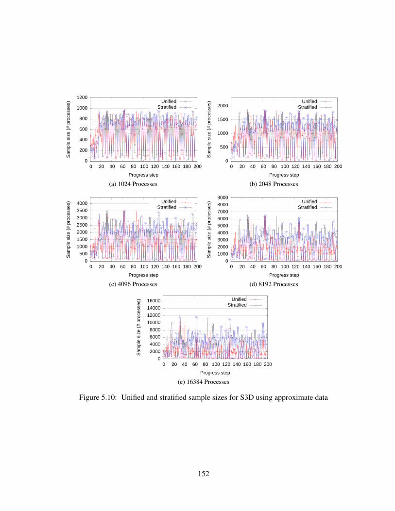
0

200

400

600

800

1000

1200

0 20 40 60 80 100 120 140 160 180 200

Sam

ple

size

(# p

roce

sses

)

Progress step

UnifiedStratified

(a) 1024 Processes

0

500

1000

1500

2000

0 20 40 60 80 100 120 140 160 180 200

Sam

ple

size

(# p

roce

sses

)

Progress step

UnifiedStratified

(b) 2048 Processes

0 500

1000 1500 2000 2500 3000 3500 4000

0 20 40 60 80 100 120 140 160 180 200

Sam

ple

size

(# p

roce

sses

)

Progress step

UnifiedStratified

(c) 4096 Processes

0 1000 2000 3000 4000 5000 6000 7000 8000 9000

0 20 40 60 80 100 120 140 160 180 200

Sam

ple

size

(# p

roce

sses

)

Progress step

UnifiedStratified

(d) 8192 Processes

0 2000 4000 6000 8000

10000 12000 14000 16000

0 20 40 60 80 100 120 140 160 180 200

Sam

ple

size

(# p

roce

sses

)

Progress step

UnifiedStratified

(e) 16384 Processes

Figure 5.10: Unified and stratified sample sizes for S3D using approximate data

152

We did not see the improvement that we expected with approximate clustering. On aver-

age, sampling cost increased by 15% to 90%, and we only improved samples for 15%-20%

of progress steps, which was not enough to yield a net gain for the entire run. This result indi-

cates that the clusterings obtained using approximate data are actually increasing the variance

in the data.

We had assumed that the MPI rank-space provided some measure of locality for sampled

data, but it appears that metric values (at least for some effort regions) are scattered through-

out this space. When we cluster at the finest possible granularity as in §5.4.3, we are able to

separate the data into reasonably homogeneous groups. Here, our sample size data indicates

that there is significant intra-neighborhood variation in our data along the process dimension.

To improve clustering accuracy, we would need further information about the locality of the

application data. Extraction of application topology is beyond the scope of this dissertation,

but it could improve these results.

5.5 Summary

In this section we described compute- and space-efficient techniques for extracting approx-

imations from compressed wavelet representations of performance data. We then described

several clustering methods, and we showed how we could use our wavelet data representation

to improve the performance of these algorithms across two dimensions of the performance

space.

We showed that we can cluster effort regions using only a very small approximation of

the original data, and that this can speed up the PAM algorithm by two to three orders of

magnitude.

We also showed that by applying scalable clustering techniques to transposed effort data

(i.e., per-process performance signatures), we could reduce the cost of sampling signifi-

153

cantly in an on-line system by stratifying the population adaptively on successive windows of

progress steps. This clustering technique integrates the sampled tracing techniques described

in Chapter 4 with the data-collection techniques described in Chapter 3. We then showed

that clustering across processes using approximate wavelet data could speed up clustering

significantly and reduce memory requirements considerably, but that we require application-

topology information to exploit this technique fully.

154

Chapter 6

Libra: A Scalable Performance Tool

6.1 Introduction

We have implemented the techniques presented in Chapters 3, 4, and 5 into Libra, a suite of

performance tools for scientific applications.

Libra consists of two main components, a client-side GUI and a suite of run-time libraries

for measuring applications. Users can link or preload our libraries with their application, and

the libraries store effort-model data to disk using either compression or sampling techniques.

The data then may be loaded into the Libra GUI for viewing and analysis.

Using the Libra GUI, one can determine which parts of the code contribute most to the

execution time of an application. A user then can zoom in on particular effort regions to

examine their load balance and effort data more closely. The GUI provides three-dimensional

visualizations of effort-model data as well as facilities for clustering similar effort regions

together.

In this chapter, we describe the software architecture of the Libra run-time libraries and

the components of its GUI client. We then give a brief example of how Libra can be used to

diagnose a real load-imbalance problem in a large-scale scientific application.

VTK Python Wrappers

VisualizationTool Kit(VTK)

Effort File Format

PyQt4 GUI

Callpath Library

Effort API

PMPI Tools

Wavelet Compression Sampled

Tracing(AMPL)

Other InstrumentationHierarchical Clustering

EZW Encoding

SWIG Python Wrappers

Callpath Library EZW Decoding

Effort API

Parallel Runtime Libraries GUI Tool

Load Balance Analysis

Figure 6.1: Libra software architecture

6.2 Software Architecture

Libra is intended for use in large-scale distributed-memory parallel systems in which very

large numbers of processes must be monitored at once. Its architecture has two main com-

ponents, as shown in Figure 6.1. First, instrumentation libraries collect data from a running

application. They then record observations using internal Libra APIs and run-time libraries.

The run-time libraries include implementations of our scalable data-collection facilities. Data

gathered is reduced and aggregated for viewing and analysis in a single client-side GUI.

6.2.1 Run-time Libraries

An instance of Libra’s run-time library is instantiated within each parallel process in moni-

tored applications. Measurements are collected at the highest level through instrumentation

libraries, which then pass the data to an intermediate Effort API. Finally, the effort API off-

loads the data internally to our scalable data-collection libraries, which record it to disk. The

run-time is a pure link-level library with the exception of progress-step instrumentation. To

use Libra, developers need only add a single function call to their progress loop, recompile,

and link statically or dynamically against our run-time libraries.

156

Effort API

The central component of Libra’s run-time libraries is the Effort API, a set of routines that

implement the effort model described in §3.2. Although users can call the effort API directly

to manually instrument code, it is intended for use by other instrumentation tools. This

way, instrumentation tools can handle the extraction of progress and effort regions from

applications, while our API handles bookkeeping for these events. Currently, we only support

extraction of effort regions using link-level MPI instrumentation.

The Effort API provides calls to indicate the completion of progress steps, as well as calls

to accumulate vectors of effort measurements for particular regions of code. For each effort

region, the user can specify custom identifiers, depending on the type of instrumentation used

and the specificity with which the application is to be measured.

Call-path Library

To simplify identification of code regions for run-time tools, we provide a C++ library with

classes for representing dynamic call paths, or call paths assessed at run time based on the call

stack. We use dynamic call paths because it is not always possible to determine the parent of a

particular call site statically. In particular, static analysis cannot handle cases in which code is

called dynamically through a function pointer or through an interrupt handler. To implement

this functionality, our call-path library uses the ParaDyn Stackwalker API (Paradyn Project,

2007). On top of this interface, we add facilities for storing, transporting, and synchronizing

call paths between processes at run-time.

Our library has special provisions for handling dynamically loaded libraries on parallel

systems. Rather than storing call sites in call paths as absolute addresses, we store (module,

offset) tuples. This describes the load module containing the call site and its offset within that

module. A call site has a single identifier regardless of which process records it, allowing

inter-process transfer of call paths in distributed memory systems.

157

Scalable Data-Collection Libraries

Data recorded using the Effort API is initially stored uncompressed in the memory of the

process in which it is observed. Internally, the API can make use of scalable data collec-

tion techniques to transmit local measurements off-node and to save them in effort-data files

viewable by the GUI. These libraries include an implementation of the effort-instrumentation

techniques discussed in §3.4, as well as the AMPL sampling library discussed in §4.3.

6.2.2 GUI Tool

Libra’s GUI allows a user to browse and analyze data collected by the run-time libraries.

It allows the user to correlate effort regions and their associated performance data with ap-

plication, as well as to visualize the data. The GUI makes use of many of the same data

representations as the instrumentation libraries to enable scalable visualization and analysis.

Common Components

The same libraries used in Libra’s run-time libraries for scalable data collection are also used

in the GUI for decompression and to represent potentially large data sets. The wavelet com-

pression and encoding libraries are used for distributed compression in the run-time libraries,

but in the GUI they are used to generate incremental, smaller-sized approximations of large

traces for display to the user. The call-path library is used on the GUI to represent identifiers

for effort regions and to correlate performance data with application source code.

These common libraries are written in C/C++, but the GUI is written primarily in Python.

To use the common libraries within Python, we generated wrappers for them using the Simple

Wrapper Interface Generator (SWIG) (Beazley, 2003). This enables us to use effort data

in GUI Python algorithms without sacrificing the performance of our encoding/decoding

algorithms or our scalable data representations.

158

GUI and Visualization

The Libra GUI is written in Python using the Qt4 library. Figure 6.2 shows a screenshot of

the main window. There are three main panels:

1. Effort browser (lower left)

2. Metric viewer (upper left)

3. Source viewer (right)

The effort browser is the starting point for Libra users. It shows data collected by the

run-time libraries hierarchically, with effort regions grouped into logical application phases.

Effort regions in the data set shown are delineated by two call paths (start and end) delineating

a dynamic region of code where effort was recorded. Initially, call paths are shown collapsed

to a single call site, but the user can expand them to see the full path and the locations of its

call sites. Figure 6.3 shows an effort region with its call paths expanded to show file and line

information from the application source code.

When the user selects an effort region in the effort browser, a plot of the load distribution

for that region is shown in the metric viewer. The plot shows effort measurements taken at

run time over all MPI processes and all progress steps. By default, the viewer shows elapsed

time, but user can customize this. She can also create more metric viewers to visualize other

data (such as HPM counter data collected using Performance API (PAPI)) simultaneously. If

the user selects multiple effort regions at once, the metric viewer will display sum of their

effort values. Likewise, if an internal node of the effort browser tree is selected, the viewer

shows the sum of all effort from its descendants. This can be used to visualize the load-

balance properties of entire phases.

Libra can also be configured to show time spent within communication operations. In

these cases, the viewer shows the single call path of the measured operation, rather than the

bounding call paths of the effort region.

159

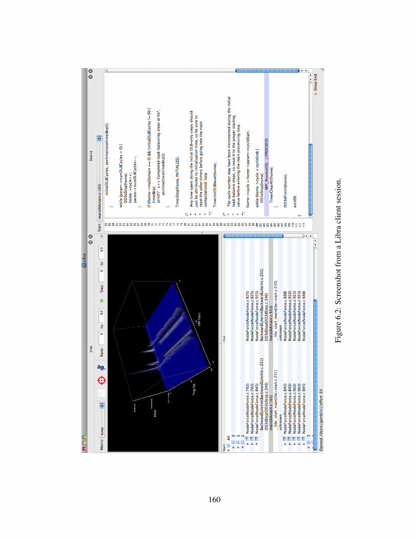
Figu

re6.

2:Sc

reen

shot

from

aL

ibra

clie

ntse

ssio

n.

160

Effort regions, labeled by deepest call sites Expanded start and end callpaths

Figure 6.3: Libra’s effort region browser, showing expanded call paths for an effort region

Highlighted callsite

Figure 6.4: Libra’s source viewer

Finally, elements in the effort browser may be sorted by the percentage of execution time

that they consume, as shown in Figure 6.5.

Libra’s source viewer highlights effort regions and call-site locations in program source

code. This enables users to correlate visualized effort data with locations in application

source code. To navigate, the user can expand call paths and select particular call sites to

show them in the source viewer. Figure 6.4 shows a highlighted call site.

Scalable Analysis

The scalable representations implemented in our data collection libraries are useful not only

in the Libra run-time, but also to generate small approximations of performance data within

the Libra GUI. With approximations, in-memory effort representations do not consume ex-

cessive memory, and clustering such data is possible on a single node. Using wavelet meth-

ods, we ensure that such approximations are low in error and that they are small enough to

enable a client node to perform analyses efficiently for very large parallel systems. Libra’s

methods of clustering effort regions by their behavior using wavelet approximations was de-

161

(a) 4,096 processes

(b) 8,192 processes

(c) 16,384 processes

Figure 6.5: Most time-consuming call sites and load-balance plots for S3D

scribed in §5.4.1.

6.3 Diagnosing Load Imbalance with Libra

We used Libra to measure the load-balance behavior of S3D (discussed in §3.5). We applied

Libra to 200-time step runs of S3D on a Blue Gene/P system (also discussed in §3.5). For

each time step, we recorded the time spent in MPI Wait and MPI Barrier, uniquely iden-

tifying each call site by its full call path with file names and line numbers for each frame. In

this case, we discovered that MPI Wait and MPI Barrier communication routines domi-

nated the run time of S3D at large scales, and that the vast majority of this time was attributed

162

to two call sites in S3D’s write savefile checkpoint routine. Since write savefile

was called from two places in the code, four call paths dominated execution time.

Figure 6.5 shows load-balance profiles reported by Libra for 4096, 8192, and 16384-

process runs of S3D on Intrepid. The tables below the profiles list the call sites and statistics

characterizing their costs. In the plots the vertical axis represents effort, the depth axis time

steps, and the horizontal axis processes. As the size of the system increases, we see large

increases in time spent in the MPI calls used by checkpointing. In all instances, the plots

show that I/O is extremely imbalanced. Because S3D writes out a checkpoint file per process,

there is contention for the I/O system. Some processes quickly write their data to disk, while

others incur contention delays to write theirs, resulting in the sawtooth-shaped load patterns

seen in the figures.

6.4 Summary

Using the novel measurement and data reduction techniques presented in this dissertation,

we have developed Libra, a full suite of performance-analysis tools. Libra consists of a set

of run-time libraries for instrumenting scientific codes, as well as a client-side GUI that can

be used to load and analyze our scalable data formats.

Using Libra, we have traced load imbalance in the S3D code to I/O contention in S3D’s

checkpoint phase, and we were able to see in detail the pattern of load imbalance across

multiple processes for runs of sizes as large as 16,384 processes. This insight has led us to

begin addressing the problem by investigating and measuring runs of S3D with alternative

I/O strategies designed to reduce and balance contention during the checkpoint phase.

163

Chapter 7

Conclusions and Future Work

Modern supercomputers are not growing smaller, and today’s systems of 100,000 or more

cores will soon give way to even larger systems with millions or more. At the time of this

writing, a 20-petaflop, 6.6-million-core machine has just been announced by Lawrence Liver-

more National Laboratory and IBM, and is expected to become operational by 2012. Within

a decade, the first exaflop machines will likely debut with even more levels of parallelism.

To understand the performance of these systems, techniques like those presented in this

dissertation will continue to be necessary. We have presented three novel systems for per-

formance monitoring, using mathematical and statistical techniques that previously had not

been applied to this domain. Our techniques were able to reduce the overhead of monitoring

and the data volume of performance measurements from large parallel applications, some-

times by two to three orders of magnitude. Our scalable representation of performance data

was viable for use on single-node systems, even for application data from runs with over

16,000 processes. Finally, we showed that single-node data analysis can be sped up using

our compact, manageable, approximate representation for performance data, and we showed

how cluster analysis can be applied to this data for further performance gains.

In this section, we give a brief summary of the main contributions and work presented in

this dissertation. We then conclude with an overview of potential future research directions

that could stem from this work.

7.1 Contributions

This dissertation made the following novel contributions to the field of large-scale parallel

performance monitoring:

• Designed a model for load-balance measurement applicable to many large-scale scien-

tific applications;

• Designed a monitoring and data-compression scheme using wavelets to achieve two

to three orders of magnitude in data reduction and nearly constant scaling behavior on

tested I/O systems;

• Designed a novel tracing technique using statistical sampling to reduce data volume of

full event traces on large systems;

• Introduced the use of an approximate wavelet representation of performance data for

fast client-side clustering, visualization, and analysis;

• Designed a scheme for on-line, run-time stratification of populations of distributed

processes into equivalence classes based on performance data using scalable clustering

techniques.

We introduced the concepts of progress and effort to divide loops in parallel applications

into two categories depending on their run-time semantics. We call this the Effort Model.

It has enabled us to represent a parallel trace across a large number of processes as three-

dimensional matrix measurements, with progress (logical steps towards completion) in one

dimension, the parallel process space in the second dimension, and regions of code in which

measurements could be made comprising the third dimension. The model is advantageous

because it is easy for application developers to understand, yet it lends itself to a wide range

of data-reduction and analysis techniques.

165

To exploit effort-model data on large systems, we devised a large-scale monitoring system

for load-balance data. Our system makes use of an entire parallel machine to compress

run-time observations speedily into a scalable, hierarchical wavelet data representation. We

showed that, using this approach, two to three orders of magnitude data of compression were

possible, along with near-constant scaling behavior on current parallel I/O architectures.

We then considered the use of population sampling to take event traces of large appli-

cations. We showed that, using traditional population-sample-size heuristics, we could limit

the amount of data necessary to monitor a parallel system, selecting a small subset of the full

set of processes. Using our technique, we achieved one to two orders of magnitude of data

reduction for parallel traces.

Finally, we combined these two performance techniques and applied scalable clustering

techniques to them for adaptive, on-line stratification of processes in parallel applications.

Our stratification techniques further reduced the cost of sampling large systems by 60% on

average, providing a useful tool to performance analysts who wish to look at the range of

behaviors among processes in parallel applications.

We have combined these techniques in the Libra parallel performance tool, which makes

use of our scalable data representations to visualize large amounts of data collected from

parallel applications on single-node client systems.

7.2 Limitations

In this section, we discuss some of the limitations of the techniques presented in the preceding

chapters, along with ideas for further improvements.

166

7.2.1 Scalable Load-Balance Measurement

The approach for scalable data collection presented in Chapter 3 is very flexible and can

be used for arbitrary numerical data. However, there are limitations to our implementation,

with potential for future improvement. First, both the effort-extraction layer and the data-

collection layer are implemented using MPI and must run synchronously within a parallel

application. We plan to update the tool to take advantage of tree-based overlay networks and

out-of-band resources so that we can collect data asynchronously as a third party outside the

application. We plan to use MRNet (Roth et al., 2003) for this functionality along with the

tool integration layer PNMPI (Schulz and de Supinski, 2007).

Progress-step instrumentation in the effort library currently is manual. The user must

insert instrumentation into application code to indicate where the transition between progress

steps occurs. While this is a simple process for most scientific codes, it is somewhat invasive.

Tools such as SimPoint (Perelman et al., 2006) and ScalaTrace (Noeth et al., 2007) provide

more robust detection of repeating behavior and phase identification in application traces.

We may be able to use tools such as these to automate progress-step instrumentation in the

future.

The current implementation of our wavelet transform only allows power-of-two process

counts in monitored MPI applications. This limitation was only included for expedient im-

plementation. We will modify our wavelet transform library slightly for future releases to

allow data collection for MPI applications of any size.

7.2.2 Statistical Sampling Techniques

AMPL is also implemented using only MPI for communication, requiring instrumentation

tools to run on-node with the parallel application. It also makes asynchronous sampling

techniques difficult. Currently, AMPL requires that updates to summary data and to sample

sets be sent on transitions between progress steps. This makes it difficult to monitor in real-

167

time applications for which the progress step may be slow. It also adds overhead because

the AMPL client code must run within a compute process. Since sampling is synchronous,

this can cause processes to wait unnecessarily. We are investigating the use of MRNet with

AMPL to solve these problems.

The traces generated by AMPL are difficult to present to the user because we currently

do not have means by which to reconstruct behavior across nodes. Users wishing to look at

AMPL’s output have two options. Either they choose representatives from within the sample

set, or they can merge the full trace and look at partial output from a group of processes. Cur-

rent viewers for TAU’s trace formats do not support viewing our sampled trace files directly,

and AMPL would need this functionality before it could be hardened into a full-fledged tool.

7.2.3 Combined Approach

Although CLARA is a fast clustering algorithm, we currently run it on a single node, and

eventually, on larger systems, even CLARA will fail to scale. In future work, we plan to

investigate distributing the CLARA algorithm to improve the speed of clustering for on-

line analysis. Since CLARA runs multiple separate instances of PAM, its parallelization is

straightforward. We could first aggregate data to a subset of the total system for analysis,

running each PAM trial separately. We could then broadcast the medoids discovered and do

theO(n) cluster assignment phase of PAM in O(log(n)) time. We reserve these improvements

for future work, but we note here that they are possible, and that the speed of CLARA is not

yet a limiting factor in the scalability of this work.

Using approximations for inter-process clustering proved less advantageous than we had

expected, but we attribute this to our lack of knowledge about application topology. We

showed that wavelet approximations are very effective in improving system-wide behavioral

clusters of effort regions because the number of regions does not change as the system grows

larger. Thus, the approximation does not discard data across the dimension on which we

168

cluster. In the future, we will investigate ways to extract information about the topology of

the process space of a parallel application and will use this to exploit locality for system-wide

behavioral clustering.

7.3 Future Research Directions

The research presented in this dissertation raises a number of new questions along with those

it has answered. This section describes future research directions that could extend the work

we have presented.

7.3.1 Topology-aware Analysis

The techniques presented in this work use stratification and hierarchical wavelet analysis to

divide processes into groups. However, we have not investigated sufficiently how best to map

these structures to the specific topologies of parallel applications. Doing so could enable us

to model more effectively application communication patterns, model distribution, and other

locality properties of large sets of parallel processes.

Topology information may also allow us to determine efficient process-to-node mappings

for simulations in which communication locality is important. Such information could be ex-

ploited using virtualization and code-motion techniques to move application processes within

a cluster in response to inferences made about an application’s topology.

Our preliminary experiment in Chapter 5 showed that the topology used for our parallel

wavelet transform could affect data compression. We have not investigated the magnitude of

this effect fully.

The Compass project used wavelet transformations to improve the power efficiency of

distributed sensor networks (Wagner et al., 2006). In this work, the authors automatically

constructed a topology based on an irregular layout of distributed sensors, and the wavelet

169

transform is performed using this layout. Our work used the MPI rank space and an S3D-

specific topology for its wavelet-transforms.

Further work is required to determine whether novel topologies can exploit locality in

effort data fully. We are also interested in whether this information can be deduced automat-

ically from performance data or from library instrumentation. MPI has support for commu-

nicators with Cartesian topology, but implementations do not guarantee that communicator

topology is mapped to the physical network topology. While the performance of this ap-

proach can be unreliable, we might be able to use the semantics to optimize our performance

tools. We will investigate deriving topology information from MPI communicators, applica-

tion communication patterns, hints from application developers, and from cluster analysis.

7.3.2 Parallel Performance Equivalence Class Detection

As mentioned, the clustering technique that we used for adaptive stratification of large appli-

cations scales well, but it required the full decompression of a window of application perfor-

mance data on a single node. This approach is not scalable. We will need to research parallel

clustering algorithms and the possibility of stratifying performance data in-situ as a parallel

application executes. This would eliminate the need for some of the aggressive aggregation

techniques presented here and would open the door to performing more sophisticated data

analysis in parallel at run time rather than on the client side.

7.3.3 Feedback-based Load-Balancing

Much of the work in this dissertation has centered around load-balance measurement, and we

plan to investigate the use of these tools to feed back load-distribution information, perfor-

mance data, and other optimization parameters to application-level load-balance algorithms.

Many parallel applications perform dynamic load-balancing, and our tools could be used in

conjunction with these to alleviate the burden of collecting performance data for application

170

developers. Using our tools, an application developer could query our monitoring system

for compact load-distribution information and use this to guide its own rebalancing routines.

Codes discussed in this dissertation, such as ParaDiS and Raptor, could make direct use of

such data as they already balance their load adaptively. Topology-aware analysis techniques

could aid in scalable description of load-redistribution parameters to these applications.

7.4 Conclusion

The work in this dissertation has made a wider range of tools available to parallel perfor-

mance analysts, and we hope that it will eventually make its way into wider use in main-

stream performance tools. We believe there is a substantial body of future research in the

area of scalable system-wide parallel performance analysis that can build on this work.

171

BIBLIOGRAPHY

Adams, M. D. (2002). The JPEG-2000 still image compression standard. Technical Report2412, ISO/IEC JTC 1/SC 29/WG.

Adams, M. D. and Kossentini, F. (2000). JasPer: a software-based JPEG-2000 codec im-plementation. In Proceedings of the International Conference on Image Processing,volume 2, pages 53–56, Vancouver, BC, Canada.

Advanced Micro Devices (2009). AMD Code Analyst,http://developer.amd.com/cpu/CodeAnalyst. Advanced Micro Devices, Inc.

Adve, V., Carle, A., Granston, E., Hiranandani, S., Kennedy, K., Koelbel, C., Kremer, U.,Mellor-Crummey, J., Warren, S., and Tseng, C.-W. (1994). Requirements for data-parallel programming environments. IEEE Parallel Distrib. Technol., 2(3):48–58.

Ahern, S., Alam, S. R., Fahey, M., Hartman-Baker, R., Barrett, R., Kendall, R., Kothe, D.,Messer, O. E., Mills, R., Sankaran, R., Tharrington, A., and White III, J. B. (2007). Sci-entific Application Requirements for Leadership Computing at the Exascale. TechnicalReport ORNL/TM-2007/238, Oak Ridge National Laboratory, Oak Ridge, Tennessee.

Ahmed, N., Natarajan, T., and Rao., K. R. (1974). Discrete cosine transform. IEEE Trans.on Computers, C(23).

Ahn, D. and Vetter, J. S. (2002). Scalable analysis techniques for microprocessor perfor-mance counter metrics. In Supercomputing 2002 (SC02), Baltimore, MD.

Ahn, D. H., Arnold, D. C., de Supinski, B. R., Lee, G. L., Miller, B. P., and Schulz, M. (2008).Overcoming scalability challenges for tool daemon launching. In Proceedings of the37th International Conference on P arallel Processing (ICPP ’08), pages 578–585,Portland, OR.

Almasi, G., Archer, C., Castanos, J. G., Gunnels, J. A., Erway, C. C., Heidelberger, P.,Martorell, X., Moreira, J. E., Pinnow, K., Ratterman, J., Steinmacher-Burow, B. D.,Gropp, W., and Toonen, B. (2005). Design and implementation of message-passingservices for the Blue Gene/L supercomputer. IBM Journal of Research and Develop-ment, 49(2/3).

Amdahl, G. (1967). Validity of the single processor approach to achieving large-scalecomputing capabilities. In American Federation of Information Processing Societies(AFIPS) Spring Joint Computer Conference, pages 483–485.

172

Anderson, J. M., Berc, L., Dean, J., Ghemawat, S., Henzinger, M., Leung, S.-T., Sites, D.,Vandevoorde, M., Waldspurger, C., and Weihl, B. (1997). Continuous profiling: Wherehave all the cycles gone? Technical Report SRC-TN-1997-016A, Digital SystemsResearch Center, Palo Alto, CA.

Ang, L.-M., Cheung, H. N., and Eshragian, K. (1999). EZW algorithm using depth-firstrepresentation of the wavelet zerotree. In Fifth International Symposium on SignalProcessing and its Applications (ISSPA), volume 1, pages 75–78, Brisbane, Australia.

Arnold, D. C., Ahn, D. H., de Supinski, B. R., Lee, G. L., Miller, B. P., and Schulz, M. (2007).Stack trace analysis for large scale debugging. In Proceedings of the InternationalParallel and Distributed Processing Symposium (IPDPS), pages 1–10, Long Beach,CA.

ASCI Program (2002). The ASCI Purple sPPM benchmark code.

Bailey, D. H., Barszcz, E., Barton, J. T., Browning, D. S., Carter, R. L., Fatoohi, R. A., Fred-erickson, P. O., Lasinski, T. A., Simon, H. D., Venkatakrishnan, V., and Weeratunga,S. K. (1991). The NAS parallel benchmarks. International Journal of SupercomputerApplications, 5(3):66–73.

Ball, D. N. (2008). Contributions of CFD to the 787 (and Future Needs). In Supercomputing2008 (SC’08), Austin, Texas.

Bandyopadhyay, S. and Coyle, E. J. (2003). An energy efficient hierarchical clustering al-gorithm for wireless sensor networks. In IEEE INFOCOM 2003, volume 3, pages1713–1723.

Barker, K., Davis, K., Hoisie, A., Kerbyson, D. J., Lang, M., Pakin, S., and Sancho, J. C.(2008). Entering the Petaflop Era: The Architecture and Performance of Roadrunner.In Supercomputing 2008 (SC’08), Austin, Texas.

Beazley, D. M. (2003). Automated scientific software scripting with swig. Future Gener.Comput. Syst., 19(5):599–609.

Boden, N. J., Cohen, D., Felderman, R. E., Kulawik, A. E., Seitz, C. L., Seizovic, J. N.,and Su, W. (1995). Myrinet - a gigabit-per-second local-area network. IEEE Micro,15:29–36.

Bordelon, A. (2007). Developing a scalable, extensible parallel performance analysis toolkit.Master’s thesis, Rice University.

Bright, A. A., Haring, R. A., Dombrowa, M. B., Omacht, M., Hoenicke, D., Singh, S.,Marcella, J. A., Lembech, R. F., Douskey, S. M., Ellavsky, M. R., Zoellin, C. G., andGara, A. (2005). Blue Gene/L compute chip; synthesis, timing, and physical design.IBM Journal of Research and Development, 49(2/3):277–287.

173

Browne, S., Dongarra, J., Garner, N., Ho, G., and Mucci, P. J. (2000). A portable program-ming interface for performance evaluation on modern processors. The InternationalJournal of High Performance Computing Applications, 14(3):189–204.

Brunst, H., Hoppe, H.-C., Nagel, W. E., and Winkler, M. (2001). Performance optimizationfor large scale computing: The scalable VAMPIR approach. In Proceedings of the 2001International Conference on Computational Science (ICCS 2001), pages 751–760, SanFrancisco, CA.

Bulatov, V., Cai, W., Hiratani, M., Hommes, G., Pierce, T., Tang, M., Rhee, M., Yates, K.,and Arsenlis, T. (2004). Scalable line dynamics in ParaDiS. In Supercomputing 2004(SC’04), pages 19–31, Pittsburgh, PA.

Cantrill, B. M., Shapiro, M. W., and Leventhal, A. H. (2004). Dynamic instrumentation ofproduction systems. In Proceedings of USENIX 2004 Annual Technical Conference,pages 15–28, Berkeley, CA, USA. USENIX Association.

Chaver, D., Prieto, M., Pinuel, L., and Tirado, F. (2002). Parallel wavelet transform for largescale image processing. In Proceedings of the 16th Annual International Parallel andDistributed Processing Symposium (IPDPS 2002), pages 4–9, Fort Lauderdale, FL.

Cheung, H. N., Ang, L.-M., and Eshraghian, K. (2000). Parallel architecture for the im-plementation of the Embedded Zerotree Wavelet algorithm. In Proceedings of the 5thAnnual Australasian Computer Architecture Conference, pages 3–8, Canberra, Aus-tralia.

Cochran, W. G. (1977). Sampling Techniques. Wiley, 3rd edition.

Colella, P., Graves, D. T., Ligocki, T. J., Martin, D. F., and Straalen, B. V. (2003a). AMRGodunov unsplit algorithm and implementation. Technical report, Applied NumericalAlgorithms Group, NERSC Division, Lawrence Berkeley National Laboratory.

Colella, P., Graves, D. T., Modiano, D., Serafini, D. B., and Straalen, B. v. (2003b). Chombosoftware package for AMR applications. Technical report, Applied Numerical Algo-rithms Group, NERSC Division, Lawrence Berkeley National Laboratory.

Colella, P., Thomas H. Dunning, J., Gropp, W. D., and Keyes, D. E., editors (2003c). AScience-Based Case for Large-Scale Simulation, volume 1, Arlington, VA. Office ofScience, U.S. Department of Energy.

Colella, P., Thomas H. Dunning, J., Gropp, W. D., and Keyes, D. E., editors (2004). AScience-Based Case for Large-Scale Simulation, volume 2, Arlington, VA. Office ofScience, U.S. Department of Energy.

Cooley, J. W. and Tukey, J. W. (1965). An algorithm for the machine calculation of complexfourier series. Mathematics of Computation, 19:297–301.

174

Crockett, R., Colella, P., Fisher, R., Klein, R. I., and McKee, C. (2005). An unsplit,cell-centered Godunov method for ideal mhd. Journal of Computional Physics,203(2):422–448.

Darema, F. (2001). The spmd model: Past, present and future. In Proceedings of the 8thEuropean PVM/MPI Users’ Group Meeting on Recent Advances in Parallel VirtualMachine and Message Passing Interface, page 1, London, UK. Springer-Verlag.

Darema-Rodgers, F., George, D., Norton, V. A., and Pfister, G. (1984). A vm parallel envi-ronment. In Proceedings of the IBM Kingston Parallel Processing Symposium.

Daubechies, I. (1992). Ten Lectures on Wavelets. Society for Industrial and Applied Mathe-matics (SIAM), Philadelphia, PA.

De Rose, L. and Reed, D. A. (2000). SvPablo: A multi-language architecture-independentperformance analysis system. In Proceedings of the 28th International Conference onParallel Processing (ICPP ’99), page 311, Fukushima, Japan.

Dean, J., Hicks, J. E., Waldspurger, C. A., Weihl, W. E., and Chrysos, G. (1997). Profileme:hardware support for instruction-level profiling on out-of-order processors. In MICRO30: Proceedings of the 30th annual ACM/IEEE international symposium on Microar-chitecture, pages 292–302, Washington, DC, USA. IEEE Computer Society.

Dongarra, J. (1987). The LINPACK benchmark: An explanation. In Houstis, E. N., Pap-atheodorou, T. S., and Polychronopoulos, C. D., editors, 1st International Conferenceon Supercomputing, pages 456–474, Athens, Greece. Springer-Verlag.

Drongowski, P. J. (2007). Instruction-based sampling: A new performance analysis techniquefor amd family 10h processors. Technical report, Advanced Micro Devices (AMD),Boston, MA.

Du, Z. and Lin, F. (2005). A novel parallelization approach for hierarchical clustering. Par-allel Comput., 31(5):523–527.

Eads, D. (2008). hcluster: Hierarchical clustering for SciPy. http://scipy-cluster.googlecode.com.

Eckart, C. and Young, G. (1936). The approximation of one matrix by another of lower rank.Psychometrika, 1(3):211–218.

Endo, T. and Matsuoka, S. (2008). Massive Supercomputing Coping with Heterogeneityof Modern Accelerators. In IEEE International Parallel & Distributed ProcessingSymposium (IPDPS 2008), April 2008.

Fenlason, J. and Stallman, R. (1988). GNU gprof: the GNU Profiler, http://ftp.gnu.org/old-gnu/Manuals/gprof-2.9.1/html mono/gprof.html. Free Software Foundation.

175

Flynn, M. J. (1972). Some computer organizations and their effectiveness. IEEE Transactionson Computers, C-21(9):948–960.

Ford, J. M., Chen, K., and Ford, N. J. (2001). Parallel implementation of fast wavelet trans-forms. Technical Report No. 389, University of Manchester, Manchester, England.

Forgy, E. W. (1965). Cluster analysis of multivariate data: efficiency vs. interpretability ofclassifications. Biometrics, 21:768–769.

Forman, G. and Zhang, B. (2000a). Distributed data clustering can be efficient and exact.SIGKDD Explor. Newsl., 2(2):34–38.

Forman, G. and Zhang, B. (2000b). Linear speedup for a parallel non-approximate recastingof centerbased clustering algorithms, including k-means, k-harmonic means, and em.Technical Report HPL-2000-158, HP Laboratories, Palo Alto, CA.

Foster, I., Kesselman, C., and Tuecke, S. (1994). The Nexus task-parallel runtime system. InIn Proc. 1st Intl Workshop on Parallel Processing, pages 457–462. Tata McGraw Hill.

Froyd, N., Mellor-Crummey, J., and Fowler, R. (2005). Low-overhead call path profiling ofunmodified, optimized code. In Proceedings of the 19th Annual International Confer-ence on Supercomputing, pages 81–90.

Froyd, N., Tallent, N., Mellor-Crummey, J., and Fowler, R. (2006). Call path profiling forunmodified, optimized binaries. In GCC Developers’ Summit, Ottawa, Canada.

Furlinger, K. and Gerndt, M. (2005). ompP: A profiling tool for OpenMP. In Proceedings ofthe First International Workshop on OpenMP (IWOMP 2005), Eugene, OR.

Gallup Organization (2009). The gallup poll, http://www.gallup.com/. On-line.

Gara, A., Blumrich, M. A., Chen, D., Chiu, G. L.-T., Coteus, P., Giampapa, M. E., Haring,R. A., Heidelberger, P., Hoenicke, D., Kopcsay, G. V., Liebsch, T. A., Ohmacht, M.,Steinmacher-Burow, B. D., Takken, T., and Vranas, P. (2005). Overview of the BlueGene/L system architecture. IBM Journal of Research and Development, 49(2/3):195–212.

Graham, S. L., Kessler, P. B., and McKusick, M. K. (1982). gprof: A call graph execu-tion profiler. In Proceedings of Programming Language Design and Impementation(PLDI), volume 17, pages 120–126.

Greenough, J., Kuhl, A., Howell, L., Shestakov, A., Creach, U., Miller, A., Tarwater, E.,Cook, A., and Cabot, B. (2003). Raptor – software and applications for BlueGene/L.In BlueGene/L Workshop. Lawrence Livermore National Laboratory.

Hartigan, J. A. and Wong, M. A. (1979). Algorithm as 136: A K-Means clustering algorithm.Applied Statistics, 28(1):100–108.

176

Hawkes, E. R. and Chen, J. H. (2004). Direct numerical simulation of hydrogen-enrichedlean premixed methane–air flames. Combustion and Flame, 138:242–258.

Hennessy, J. L. and Patterson, D. A. (2006a). Computer Architecture, chapter 5: MemoryHierarchy Design. Morgan Kaufman, 4th edition.

Hennessy, J. L. and Patterson, D. A. (2006b). Computer Architecture, chapter 2: Instruction-level Parallelism. Morgan Kaufman, 4th edition.

Hoefler, T., Schneider, T., and Lumsdaine, A. (2008). Multistage switches are not cross-bars: Effects of static routing in high-performance networks. In IEEE InternationalConference on Cluster Computing, pages 116–125, Tsukuba, Japan.

Hollingsworth, J. K. (1994). Finding Bottlenecks in Large-scale Parallel Programs. Ph.D.dissertation, University of Wisconsin-Madison.

Hopke, P. K. (1990). The application of supercomputer to chemometrics. In Karjalainen,E. J., editor, Proceedings of the Scientific Computing and Automation (Europe) Con-ference, Masstricht, The Netherlands.

Huck, K. A. and Malony, A. D. (2005). PerfExplorer: A performance data mining frameworkfor large-scale parallel computing. In Supercomputing 2005 (SC’05), page 41, Seattle,WA.

Huffman, D. A. (1952). A method for the construction of minimum-redundancy codes. Pro-ceedings of the Institute of Radio Engineers, 40(9):1098–1101.

IBM Rational Software (2009). IBM Rational Purify, http://www.ibm.com/software/rational.International Business Machines Corporation.

IEEE (2005). IEEE 802.3 LAN/MAN CSMA/CD Access Method. Ethernet in the First Mile.IEEE Computer Society, 345 E. 47th St, New York, NY 10017, USA.

Kamath, C., Baldwin, C. H., Fodor, I. K., and Tang, N. A. (2000). On the design andimplementation of a parallel, object-oriented, image processing toolkit. In Paralleland Distributed Methods for Image Processing IV, SPIE annual meeting.

Karavanic, K. L. (2000). Experiment management support for parallel performance tuning.PhD thesis, University of Wisconsin-Madison. Supervisor-Miller, Barton P.

Karypis, G. and Kumar, V. (1998). A fast and high quality multilevel scheme for partitioningirregular graphs. SIAM Journal on Scientific Computing, 20(1):359–392.

Kaufman, L., Hopke, P. K., and Rousseeuw, P. J. (1988). Using a parallel computer systemfor statistical resampling methods. Computational Statistics Quarterly, 2:129–141.

Kaufman, L. and Rousseeuw, P. J. (2005a). Finding Groups in Data: An Introduction toCluster Analysis, chapter 5, pages 199–252. Wiley Series in Probability and Statistics.Wiley-Interscience, 2nd edition.

177

Kaufman, L. and Rousseeuw, P. J. (2005b). Finding Groups in Data: An Introduction toCluster Analysis, chapter 3, pages 126–163. Wiley Series in Probability and Statistics.Wiley-Interscience, 2nd edition.

Kaufman, L. and Rousseeuw, P. J. (2005c). Finding Groups in Data: An Introduction toCluster Analysis, chapter 2, pages 68–125. Wiley Series in Probability and Statistics.Wiley-Interscience, 2nd edition.

Kaufman, L. and Rousseeuw, P. J. (2005d). Finding Groups in Data: An Introduction toCluster Analysis. Wiley Series in Probability and Statistics. Wiley-Interscience, 2ndedition.

Kumar, S. and Kale, L. V. (2004). Scaling all-to-all multicast on fat-tree networks. In ICPADS’04: Proceedings of the Tenth International Conference on Parallel and DistributedSystems, page 205, Washington, DC, USA. IEEE Computer Society.

Kutil, R. (2002). Approaches to zerotree image and video coding on MIMD architectures.Parallel Computing, 28(7-8):1095–1109.

Lee, G. L., Ahn, D. H., Arnold, D. C., de Supinski, B. R., Legendre, M., Miller, B. P., Schulz,M., and Liblit, B. (2008). Lessons learned at 208k: towards debugging millions ofcores. In SC ’08: Proceedings of the 2008 ACM/IEEE conference on Supercomputing,pages 1–9, Piscataway, NJ, USA. IEEE Press.

Leiserson, C. E. (1985). Fat-trees: universal networks for hardware-efficient supercomputing.IEEE Trans. Comput., 34(10):892–901.

Levon, J. and Elie, P. (2008). Oprofile manual, http://oprofile.sourceforge.net/doc.

Liao, C., Hernandez, O., Chapman, B., Chen, W., and Zheng, W. (2007). Openuh: an op-timizing, portable openmp compiler: Research articles. Concurr. Comput. : Pract.Exper., 19(18):2317–2332.

Lloyd, S. P. (1967, 1982). Least squares quantization in PCM. technical note, Bell Labora-tories. IEEE Transactions on Information Theory, 28:128–137.

Louis, S. and de Supinski, B. R. (2005). BlueGene/L: Early application scaling results.In NNSA ASC Principal Investigator Meeting & BG/L Consortium System SoftwareWorkshop, Salt Lake City, Utah.

Lu, C.-d. and Reed, D. A. (2002). Compact application signatures for parallel and distributedscientific codes. In Supercomputing 2002 (SC02), pages 1–10, Baltimore, MD.

Luettich, R., Westerink, J., and Scheffner, N. (1992). ADCIRC: an advanced three-dimensional circulation model for shelves coasts and estuaries, Report 1: theory andmethodology of ADCIRC-2DDI and ADCIRC-3DL. Dredging Research ProgramTechnical Report DRP-92-6, U.S. Army Engineers Waterways Experiment Station,Vicksburg, MS.

178

MacQueen, J. (1967). Some methods for classification and analysis of multivariate obser-vations. In Cam, L. M. L. and Neyman, J., editors, Proceedings of the Fifth Berke-ley Symposium on Mathematical Statistics and Probability, volume 1, pages 281–297.Univeristy of California Press.

Mascagni, M. and Srinivasan, A. (2000). Algorithm 806: SPRNG: A scalable library forpseudorandom number generation. ACM Transactions on Mathematical Software,26:436–461.

Meerwald, P., Norcen, R., and Uhl, A. (2002). Parallel JPEG2000 image coding on multi-processors. In Proceedings of the 16th Annual International Parallel and DistributedProcessing Symposium (IPDPS 2002), page 248, Fort Lauderdale, FL.

Meila, M. (2005). Comparing clusterings: an axiomatic view. In Proceedings of the 22nd In-ternational Conference on Machine Learning (ICML ’05), pages 577–584, New York,NY, USA. ACM.

Mellor-Crummey, J. (2003). HPCToolkit: Multi-platform tools for profile-based perfor-mance analysis. In 5th International Workshop on Automatic Performance Analysis(APART).

Mendes, C. L. and Reed, D. A. (1998). Integrated compilation and scalability analysis forparallel systems. In International Conference on Parallel Architectures and Compila-tion Techniques, pages 385–392, Paris, France.

Mendes, C. L. and Reed, D. A. (2004). Monitoring large systems via statistical sampling.International Journal of High Performance Computing Applications, 18(2):267–277.

Metcalfe, R. M., Boggs, D. R., Thacker, C. P., and Lampson, B. W. (1977). Multipoint datacommunication system with collision detection. U.S. Patent 4,063,220.

Meuer, H., Strohmaier, E., Dongarra, J., and Horst, S. (2009). ”Top500 SupercomputerSites”.

Michalakes, J. G. (2002). Weather research and forecasting model: Design and implementa-tion. Technical report, Internal Draft Documentation.

Miller, B. P., Callaghan, M. D., Cargille, J. M., Hollingsworth, J. K., Irvin, R. B., Karavanic,K. L., Kunchithapadam, K., and Newhall, T. (1995). The Paradyn parallel performancemeasurement tools. IEEE Computer, 28(11: Special issue on performance evaluationtools for parallel and distributed computer systems.):37–46.

Mirkin, B. (1996). Mathematical Classification and Clustering. Kluwer Academic Publish-ers.

Mohr, B., Malony, A. D., Shende, S., and Wolf, F. (2001). Towards a performance toolinterface for openmp: An approach based on directive rewriting. In Proceedings of theThird Workshop on OpenMP (EWOMP’01).

179

Moore, G. (1965). Cramming more components onto integrated circuits. Electronics, 38(8).

Morton, G. M. (1966). A computer oriented geodetic data base and a new technique in filesequencing. Technical report, IBM Ltd., Ottawa, Ontario.

MPI Forum (1994). MPI: A message passing interface standard. International Journal ofSupercomputer Applications and High Performance Computing, 8(3/4):159–416.

Murtagh, F. (1985). Multidimensional Clustering Algorithms. Physica-Verlag.

Navier, C. L. M. H. (1822). Memoire sur les lois du mouvement des fluides. Memoires del’Academie Royale des Sciences de l’Institut de France, 6:389–440.

Nethercote, N. and Seward, J. (2007). Valgrind: a framework for heavyweight dynamicbinary instrumentation. SIGPLAN Notices, 42(6):89–100.

Nielsen, O. M. and Hegland, M. (2000). Parallel performance of fast wavelet transform.International Journal of High Speed Computing, 11(1):55–73.

Nikolayev, O. Y., Roth, P. C., and Reed, D. A. (1997). Real-time statistical clustering forevent trace reduction. The International Journal of Supercomputer Applications andHigh Performance Computing, 11(2):144–159.

Noeth, M., Mueller, F., Schulz, M., and de Supinski, B. R. (2007). Scalable compression andreplay of communication traces in massively parallel environments. In Proceedings ofthe 21st Annual International Parallel and Distributed Processing Symposium (IPDPS2007), pages 1–11, Long Beach, CA.

Olson, C. F. (1993). Parallel algorithms for hierarchical clustering. Parallel Computing,21:1313–1325.

on behalf of the USQCD Collaboration, B. J. (2008). Continuing progress on a lattice qcdsoftware infrastructure. In J. Phys. Conference Series, volume 125.

Paradyn Project (2007). DynStackwalker Programmer’s Guide. Madison, WI. Version 0.6b.

Parsons, L., Haque, E., and Liu, H. (2004). Subspace clustering for high dimensional data: areview. SIGKDD Explor. Newsl., 6(1):90–105.

Pearson, K. (1901). On lines and planes of closest fit to systems of points in space. Philo-sophical Magazine, 2(6):559–572.

Perelman, E., Polito, M., Bouget, J.-Y., Sampson, J., Calder, B., and Dulong, C. (2006).Detecting phases in parallel applications on shared memory architectures. In Proceed-ings of the 20th Annual International Parallel and Distributed Processing Symposium(IPDPS 2006), Rhodes, Greece.

180

Pivkin, I., Richardson, P., and Karniadakis, G. (2006). Blood flow velocity effects and roleof activation delay time on growth and form of platelet thrombi. In Proc Nat Acad Sci103(46):, pages 17164–17169.

Pivkin, I., Richardson, P., Laidlaw, D. H., and Karniadakis, G. (2005). Combined effects ofpulsatile flow and dynamic curvature on wall shear stress in a coronary artery bifurca-tion model. Journal of Biomechanics, 38(6):1283–1290.

Rajasekaran, S. (2005). Efficient parallel hierarchical clustering algorithms. IEEE Transac-tions on Parallel and Distributed Systems, 16(6):497–502.

Ramanathan, R. M. (2006). White Paper: Extending the World’s Most Popular ProcessorArchitecture. Technical report, Intel Corporation.

Ranka, S. and Sahni, S. (1991). Clustering on a hypercube multicomputer. IEEE Trans.Parallel Distrib. Syst., 2(2):129–137.

Ratn, P., Mueller, F., de Supinski, B. R., and Schulz, M. (2008). Preserving time during com-pression and replay of large-scale communication traces. In Proceedings of the 22ndInternational Conference on Supercomputing (ICS ’08), pages 46–55, Kos, Greece.

Ribler, R., Vetter, J., Simitci, H., Simitci, H., and Reed, D. A. (1998). Autopilot: Adaptivecontrol of distributed applications. In Proceedings of the 7th IEEE Symposium onHigh-Performance Distributed Computing, pages 172–179.

Richardson, P., Pivkin, I., and Karniadakis, G. (2008). Red cells in shear flow: Dissipativeparticle dynamics modeling. Biorheology, 45:107–108.

Rissanen, J. J. and G. G. Langdon, J. (1979). Arithmetic coding. IBM Journal of Researchand Development, 23(2):149–162.

Ross, R., Moreira, J., Cupps, K., and Pfeiffer, W. (2006). Parallel I/O on the IBM BlueGene/L system. Blue Gene/L Consortium Quarterly Newsletter, First Quarter.

Roth, P. C. (1996). Etrusca: Event trace reduction using statistical data clustering analysis.Master’s thesis, University of Illinois at Urbana-Champaign.

Roth, P. C. (2005). Scalable On-line Automated Performance Diagnosis. Ph.D. dissertation,University of Wisconsin-Madison.

Roth, P. C., Arnold, D. C., and Miller, B. P. (2003). MRNet: A software-based multi-cast/reduction network for scalable tools. In Supercomputing 2003 (SC’03), Phoenix,AZ.

Roth, P. C. and Miller, B. P. (2006). On-line automated performance diagnosis on thousandsof processors. In Proceedings of the ACM SIGPLAN Symposium on Principles andPractice of Parallel Programming (PPoPP’06), pages 69–80, New York, NY.

181

Russell, R. M. (1978). The CRAY-1 computer system. Communications of the ACM,21(1):63–72.

Schaeffer, R. L., Mendenhall, W., and Ott, R. L. (2006). Elementary Survey Sampling.Wadsworth Publishing Co., Belmont, CA, 6th edition.

Schmuck, F. and Haskin, R. (2002). GPFS: A shared-disk file system for large computingclusters. In Proceedings of the FAST’02 Conference on File and Storage Technologies,Monterey, CA.

Schulz, M. and de Supinski, B. R. (2007). PNMPI tools: A whole lot greater than the sum oftheir parts. In Supercomputing 2007 (SC’07), Reno, NV.

SGI (2003). SpeedShop user’s guide. Technical Report 007-3311-0011, Silicon Graphics,Inc. (SGI).

Shanley, T. (2002). Infiniband. Addison-Wesley Longman Publishing Co., Inc., Boston, MA,USA.

Shannon, C. E. (1948). A mathematical theory of communication. The Bell Systems Techni-cal Journal, 27:379–423.

Shapiro, J. M. (1993). Embedded image coding using zerotrees of wavelet coefficients. IEEETransactions on Signal Processing, 41(12):3445–3462.

Sheikholeslami, G., Chatterjee, S., and Zhang, A. (2000). Wavecluster: A wavelet-basedclustering approach for spatial data in very large databases. In The VLDB Journal,volume 8, pages 289–304.

Shende, S. and Maloney, A. (2006). The TAU parallel performance system. InternationalJournal of High Performance Computing Applications, 20(2):287–331.

Sherwood, T., Perelman, E., Hamerly, G., and Calder, B. (2002). Automatically characteriz-ing large scale program behavior. In Tenth International Conference on ArchitecturalSupport for Programming Languages and Operating Systems (ASPLOS-X), pages 45–47, San Jose, CA.

Sherwood, T., Perelman, E., Hamerly, G., Sair, S., and Calder, B. (2003). Discovering andexploiting program phases. IEEE Micro: Micro’s Top Picks from Computer Architec-ture Conferences.

Snavely, A., Wolter, N., and Carrington, L. (2001). Modeling application performance byconvolving machine signatures with application profiles. In IEEE Workshop on Work-load Characterization, 2001.

Spearman, C. (1904). General intelligence, objectively determined and measured. AmericanJournal of Psychology, 15:201–293.

182

Spicka, P. and Grald, E. (2004). The role of computational fluid dynamics (CFD) in hairscience. In International Conference on Applied Hair Science, volume 55, pages S53–S63. Society of Cosmetic Chemists, New York, NY.

Stoffel, K. and Belkoniene, A. (1999). Parallel k/h -means clustering for large data sets. InProceedings of EuroPar ’99, pages 1451–1454.

Stokes, G. G. (1845). On the theories of internal friction of fluids in motion. Transactions ofthe Cambridge Philosophical Society, 8:287–305.

Tamches, A. and Miller, B. P. (1999). Fine-grained dynamic instrumentation of commod-ity operating system kernels. In OSDI ’99: Proceedings of the Third Symposium onOperating Systems Design and Implementation, pages 117–130, Berkeley, CA, USA.USENIX Association.

U.S. Census Bureau (2009). Census Bureau Home Page, http://www.census.gov/. On-line.

Valiant, L. G. (1990). A bridging model for parallel computation. Communications of theACM, 33(8):103–111.

Vetter, J. and Chambreau, C. (2005). mpiP: Lightweight, scalable mpi profiling.

Vetter, J. S., Alam, S. R., Dunigan, Jr., T. H., Fahey, M. R., Roth, P. C., and Worley, P. H.(2006). Early evaluation of the Cray XT3. In Proceedings of the 20th InternationalParallel and Distributed Processing Symposium (IPDPS), Rhodes, Greece.

Wagner, R. S., Baraniuk, R. G., Du, S., Johnson, D. B., and Cohen, A. (2006). An architecturefor distributed wavelet analysis and processing in sensor networks. In InformationProcessing in Sensor Networks (IPSN06), pages 243–250, New York, NY, USA. ACMPress.

Walnut, D. F. (2004). An Introduction to Wavelet Analysis. Birkhauser Boston.

Wang, B., Ding, Q., and Rahal, I. (2008). Parallel hierarchical clustering on market basketdata. In ICDMW ’08: Proceedings of the 2008 IEEE International Conference on DataMining Workshops, pages 526–532, Washington, DC, USA. IEEE Computer Society.

Wang, J., Adve, V. S., Mellor-Crummey, J., Anderson, M., Kennedy, K., and Reed, D. A.(1995). An integrated compilation and performance analysis environment for dataparallel programs. In in Proceedings of Supercomputing ’95, pages 1370–1404.

Weinberg, J. and Snavely, A. E. (2008). Accurate memory signatures and synthetic addresstraces for hpc applications. In ICS ’08: Proceedings of the 22nd Annual InternationalConference on Supercomputing, pages 36–45, New York, NY, USA. ACM.

Welch, T. A. (1984). A technique for high-performance data compression. Computer,17(6):8–19.

183

Wheeler, D. A. (2002). More than a gigabuck: Estimating GNU/Linux’s size,http://www.dwheeler.com/sloc/redhat71-v1/redhat71sloc.html. On-line.

184